Embed Size (px)
Citation preview
Akewak Jeba
Digital Image Processing
and Image Restoration
Helsinki Metropolia University of Applied Sciences Bachelor of Engineering
Information Technology Thesis May 5, 2011
2
Abstract
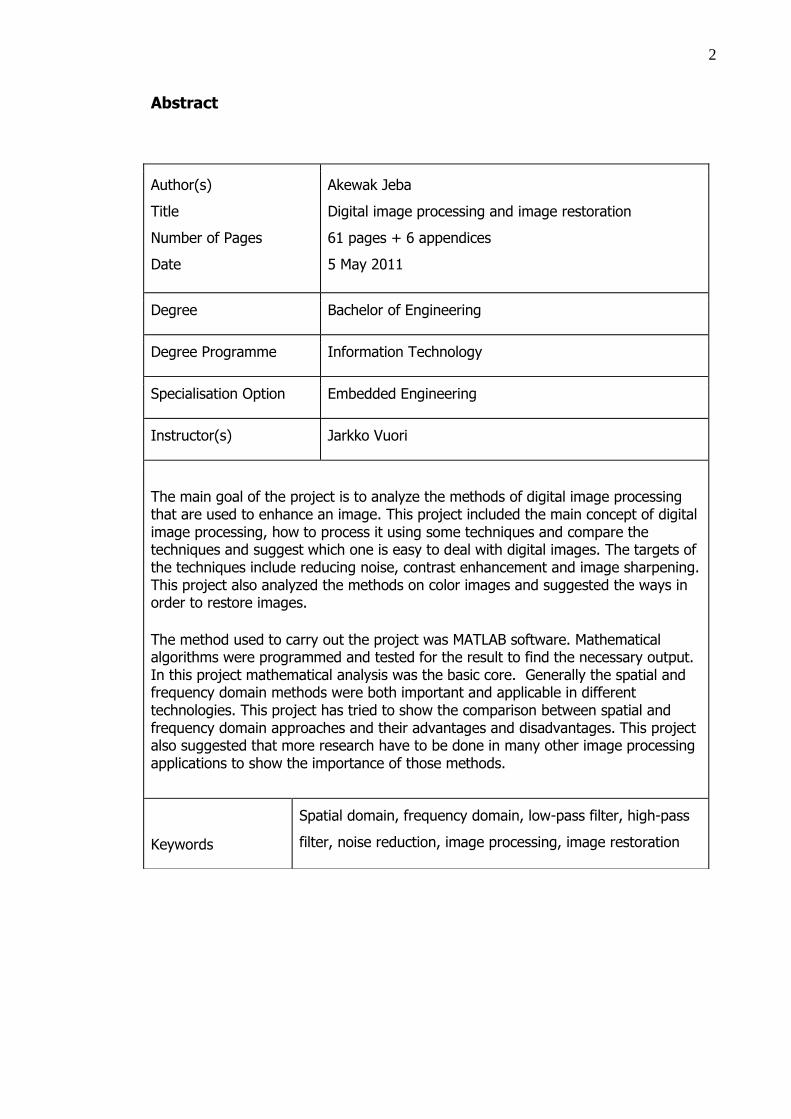
Author(s)
Title
Number of Pages
Date
Akewak Jeba
Digital image processing and image restoration
61 pages + 6 appendices
5 May 2011
Degree Bachelor of Engineering
Degree Programme Information Technology
Specialisation Option Embedded Engineering
Instructor(s) Jarkko Vuori
The main goal of the project is to analyze the methods of digital image processing that are used to enhance an image. This project included the main concept of digital image processing, how to process it using some techniques and compare the techniques and suggest which one is easy to deal with digital images. The targets of the techniques include reducing noise, contrast enhancement and image sharpening. This project also analyzed the methods on color images and suggested the ways in order to restore images. The method used to carry out the project was MATLAB software. Mathematical algorithms were programmed and tested for the result to find the necessary output. In this project mathematical analysis was the basic core. Generally the spatial and frequency domain methods were both important and applicable in different technologies. This project has tried to show the comparison between spatial and frequency domain approaches and their advantages and disadvantages. This project also suggested that more research have to be done in many other image processing applications to show the importance of those methods.
Keywords
Spatial domain, frequency domain, low-pass filter, high-pass
filter, noise reduction, image processing, image restoration
3
Contents
Abstract ............................................................................................................................ 2
Table of Symbols ............................................................................................................ 5
1 Introduction .................................................................................................................. 6
2 Theoretical Background .............................................................................................. 7
2.1 Fundamentals of Digital Image Processing ...................................................... 7
2.2 Basics of Image Sampling and Quantization ................................................... 8
3 Spatial Domain Image Enhancement and Transformation ................................. 10
3.1 Gray Level Transformation ............................................................................... 10
3.2 Histogram Processing ........................................................................................ 13
3.2.1 Histogram Representation ......................................................................... 13
3.2.2 Histogram Equalization .............................................................................. 14
3.2.3 Histogram Matching ................................................................................... 18
3.3 Image Subtraction ............................................................................................. 18
3.4 Image Averaging ................................................................................................ 20
3.5 Spatial Filtering ................................................................................................... 22
3.6 Smoothing Spatial Filter .................................................................................... 22
3.7 Median Filtering .................................................................................................. 24
3.8 Sharpening Spatial Filter ................................................................................... 26
3.8.1 The Laplacian Method ................................................................................ 27
3.8.2 The Gradient Method ................................................................................. 29
4 Frequency Domain Image Enhancement............................................................... 31
4.1 Fourier Transform .............................................................................................. 31
4.2 The Discrete Fourier Transform ....................................................................... 31
4.3 Smoothing Frequency Domain Filter ............................................................... 34
4.3.1 Ideal Low-pass Filter .................................................................................. 34
4.3.2 Butterworth Low-pass Filter ...................................................................... 37
4.4 Sharpening in Frequency Domain ................................................................... 38
4
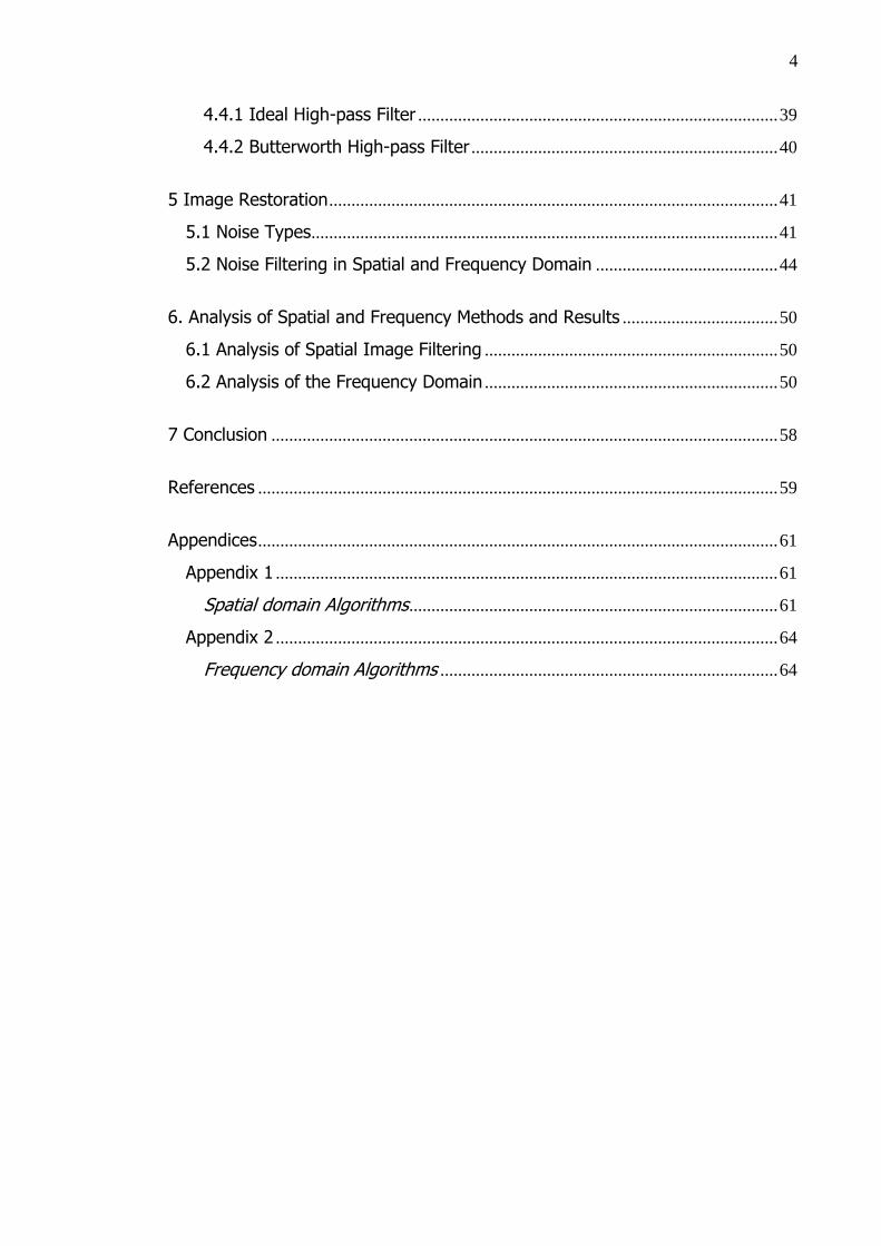
4.4.1 Ideal High-pass Filter ................................................................................. 39
4.4.2 Butterworth High-pass Filter ..................................................................... 40
5 Image Restoration ..................................................................................................... 41
5.1 Noise Types ......................................................................................................... 41
5.2 Noise Filtering in Spatial and Frequency Domain ......................................... 44
6. Analysis of Spatial and Frequency Methods and Results ................................... 50
6.1 Analysis of Spatial Image Filtering .................................................................. 50
6.2 Analysis of the Frequency Domain .................................................................. 50
7 Conclusion .................................................................................................................. 58
References ..................................................................................................................... 59
Appendices ..................................................................................................................... 61
Appendix 1 ................................................................................................................. 61
Spatial domain Algorithms ................................................................................... 61
Appendix 2 ................................................................................................................. 64
Frequency domain Algorithms ............................................................................ 64
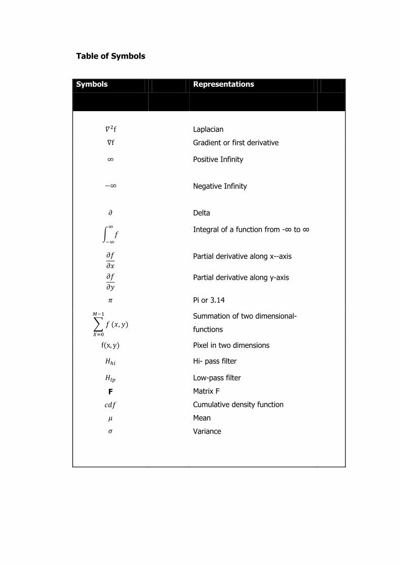
Table of Symbols
Symbols Representations
Laplacian
Gradient or first derivative
Positive Infinity
Negative Infinity
Delta
Integral of a function from -∞ to ∞
Partial derivative along x--axis
Partial derivative along y-axis
Pi or 3.14
Summation of two dimensional-
functions
Pixel in two dimensions
Hi- pass filter
F
Low-pass filter
Matrix F
Cumulative density function
Mean
Variance
6
1 Introduction
The main goal of this thesis is to show how a digital image is being processed and
as the result to have a better quality picture. The digital images are going to be
enhanced using spatial and frequency domain methods.
The images are going to be enhanced with the above mentioned methods and
those methods have their own approaches. However all they do is enhancing an
image with a better quality. The main targets of the techniques mentioned above
include noise reduction, contrast enhancement and image sharpening. In this thesis
I am going to discuss those targets in brief.
This topic is chosen to show the importance in our real life such as in Medical
fields, astronomy, forensics, photography, game industry, and biological
researches. Image processing is the core of many scientific researches and fields.
But nowadays the image processing is implemented using digital systems such as
simple computer chips. Therefore certain digital image processing approaches and
methods are needed in order to processes those digital images. Here the project
has tried to implement some of the methods.
7
2 Theoretical Background
In this background section the fundamentals of digital image processing and the basic
concepts of image and its representation are discussed.
2.1 Fundamentals of Digital Image Processing
Image processing deals with analysis of images using different techniques. Image
processing deals with the any action to change an image. Image processing has
different methods like optical, analog and digital image processing. Digital image
processing is a part of signal processing where we processes digital images using
computer algorithms. The computer algorithms can be modified so that we can also
change the appearance of the digital image easily and quickly.
Digital image processing has numerous applications in different studies and researches
of science and technology. Some of fields that use digital image processing include:
biological researches, finger print analysis in forensics, medical fields, photography and
publishing fields, astronomy, and in the film and game industries.
Digital image processing has fundamental classes which are grouped depending on
their operations:
a. Image enhancement: image enhancement deals with contrast enhancement,
spatial filtering, frequency domain filtering, edge enhancement and noise
reduction. This project briefly shows the theoretical and practical approaches.
b. Image restoration: in this class the image is corrected using different correction
methods like inverse filtering and feature extraction in order to restore an
image to its original form.
c. Image analysis: image analysis deals with the statistical details of an image.
Here it is possible to examine the information of an image in detail. This
information helps in image restoration and enhancement. One of the
representations of the information is the histogram representation to show the
brightness and darkness in order to arrange and stretch the images to have an
enhanced image relative to the original image. During image analysis the main
tasks include image segmentation, feature extraction and object classification.
8
d. Image compression: image compression deals with the compression of the size
of the image so that it can easily be stored electronically. The compressed
images are then decompressed to their original forms. Here the image
compression and decompression can either lose their size by maintaining high
quality or preserves the original data size without losing size.
e. Image synthesis: this class of digital image processing is well known nowadays
in the film and game industry. Nowadays the film and game industry is very
advanced in 3-dimensional and 4-dimensional productions. In both cases the
images and videos scenes are constructed using certain techniques. The image
synthesis has two forms tomography and visualization. [3]
2.2 Basics of Image Sampling and Quantization
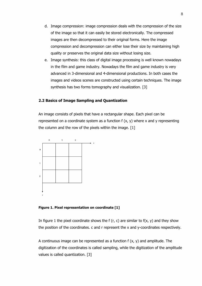
An image consists of pixels that have a rectangular shape. Each pixel can be
represented on a coordinate system as a function f (x, y) where x and y representing
the column and the row of the pixels within the image. [1]
Figure 1. Pixel representation on coordinate [1]
In figure 1 the pixel coordinate shows the f (r, c) are similar to f(x, y) and they show
the position of the coordinates. c and r represent the x and y-coordinates respectively.
A continuous image can be represented as a function f (x, y) and amplitude. The
digitization of the coordinates is called sampling, while the digitization of the amplitude
values is called quantization. [3]
9
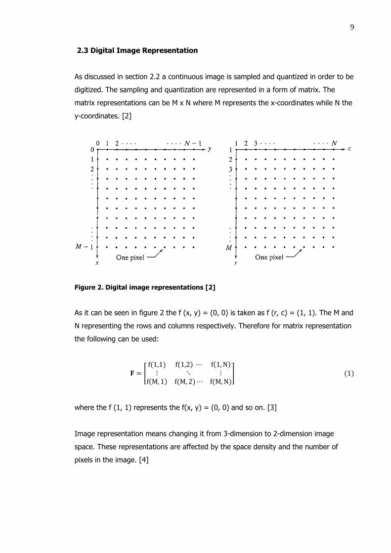
2.3 Digital Image Representation
As discussed in section 2.2 a continuous image is sampled and quantized in order to be
digitized. The sampling and quantization are represented in a form of matrix. The
matrix representations can be M x N where M represents the x-coordinates while N the
y-coordinates. [2]
Figure 2. Digital image representations [2]
As it can be seen in figure 2 the f (x, y) = (0, 0) is taken as f (r, c) = (1, 1). The M and
N representing the rows and columns respectively. Therefore for matrix representation
the following can be used:
where the f (1, 1) represents the f(x, y) = (0, 0) and so on. [3]
Image representation means changing it from 3-dimension to 2-dimension image
space. These representations are affected by the space density and the number of
pixels in the image. [4]
10
3 Spatial Domain Image Enhancement and Transformation
3.1 Gray Level Transformation
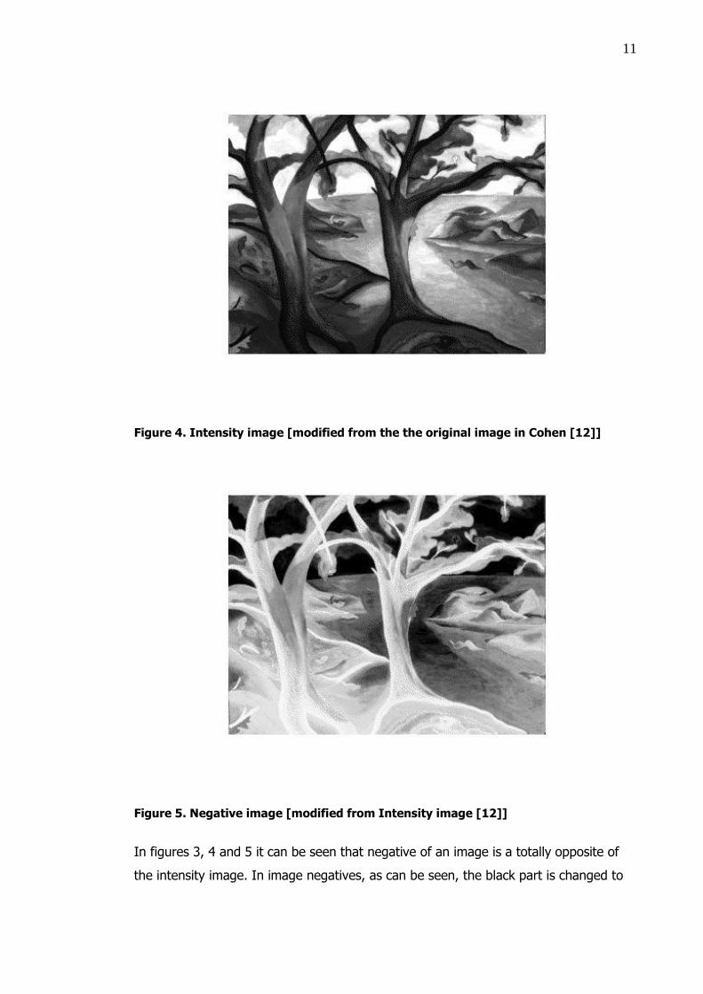
In gray level transformation there are many forms of functions in image enhancement.
Among them are linear, logarithmic, and power transformations. In linear
transformations the image functions are linear functions. [3] One example is Image
negative. During image negation we have an intensity image of the form that is shown
below in the following figures 4 and 5. Intensity image can be gray scale image and it
represents an image as a matrix where it shows how bright or dark the pixel at the
corresponding position should be colored.
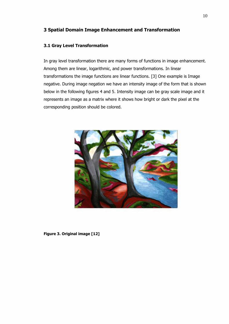
Figure 3. Original image [12]
11
Figure 4. Intensity image [modified from the the original image in Cohen [12]]
Figure 5. Negative image [modified from Intensity image [12]]
In figures 3, 4 and 5 it can be seen that negative of an image is a totally opposite of
the intensity image. In image negatives, as can be seen, the black part is changed to
12
white while the white is also to black. This is used for enhancing a white detail
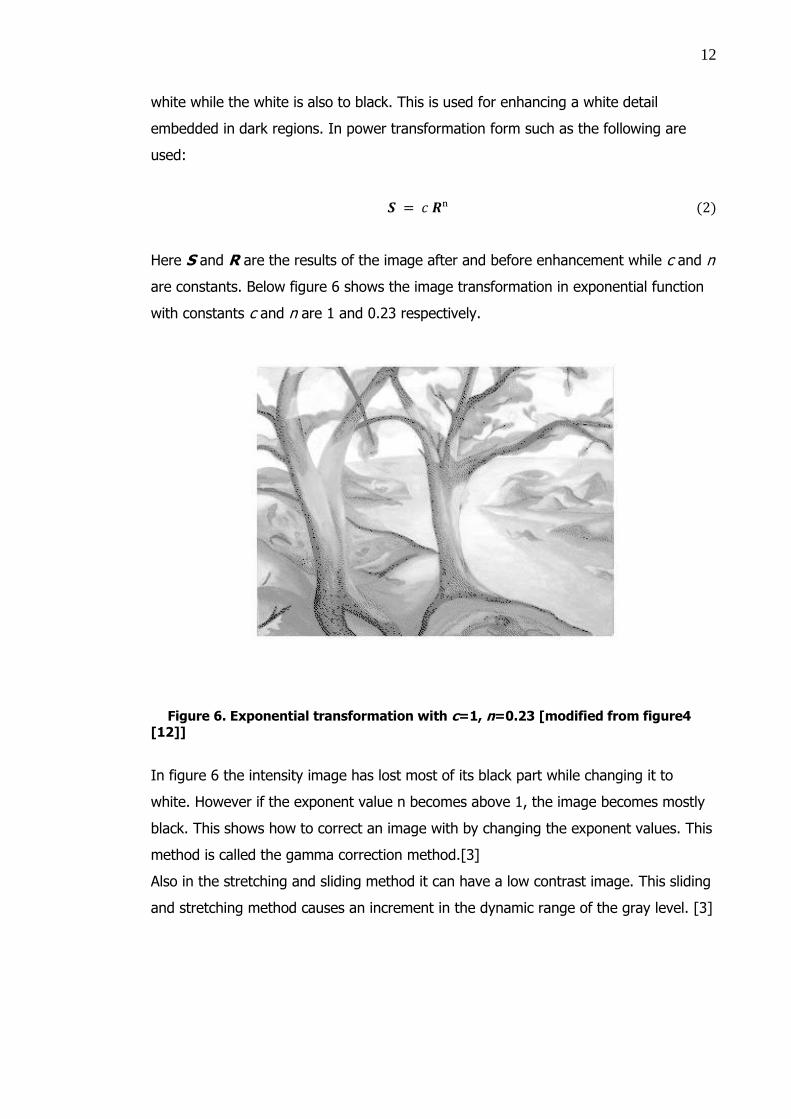
embedded in dark regions. In power transformation form such as the following are
used:
Here S and R are the results of the image after and before enhancement while c and n
are constants. Below figure 6 shows the image transformation in exponential function
with constants c and n are 1 and 0.23 respectively.
Figure 6. Exponential transformation with c=1, n=0.23 [modified from figure4
[12]]
In figure 6 the intensity image has lost most of its black part while changing it to
white. However if the exponent value n becomes above 1, the image becomes mostly
black. This shows how to correct an image with by changing the exponent values. This
method is called the gamma correction method.[3]
Also in the stretching and sliding method it can have a low contrast image. This sliding
and stretching method causes an increment in the dynamic range of the gray level. [3]
13
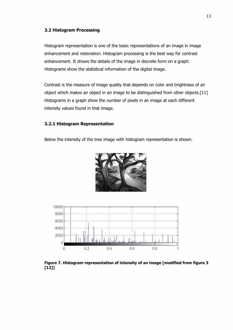
3.2 Histogram Processing
Histogram representation is one of the basic representations of an image in image
enhancement and restoration. Histogram processing is the best way for contrast
enhancement. It shows the details of the image in discrete form on a graph.
Histograms show the statistical information of the digital image.
Contrast is the measure of image quality that depends on color and brightness of an
object which makes an object in an image to be distinguished from other objects.[11]
Histograms in a graph show the number of pixels in an image at each different
intensity values found in that image.
3.2.1 Histogram Representation
Below the intensity of the tree image with histogram representation is shown.
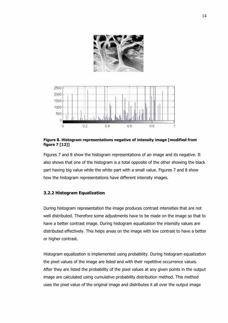
Figure 7. Histogram representation of intensity of an image [modified from figure 3
[12]]
14
Figure 8. Histogram representations negative of intensity image [modified from
figure 7 [12]]
Figures 7 and 8 show the histogram representations of an image and its negative. It
also shows that one of the histogram is a total opposite of the other showing the black
part having big value while the white part with a small value. Figures 7 and 8 show
how the histogram representations have different intensity images.
3.2.2 Histogram Equalization
During histogram representation the image produces contrast intensities that are not
well distributed. Therefore some adjustments have to be made on the image so that to
have a better contrast image. During histogram equalization the intensity values are
distributed effectively. This helps areas on the image with low contrast to have a better
or higher contrast.
Histogram equalization is implemented using probability. During histogram equalization
the pixel values of the image are listed and with their repetitive occurrence values.
After they are listed the probability of the pixel values at any given points in the output
image are calculated using cumulative probability distribution method. This method
uses the pixel value of the original image and distributes it all over the output image
15
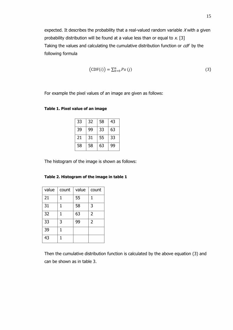
expected. It describes the probability that a real-valued random variable X with a given
probability distribution will be found at a value less than or equal to x. [3]
Taking the values and calculating the cumulative distribution function or cdf by the
following formula
)
For example the pixel values of an image are given as follows:
Table 1. Pixel value of an image
33 32 58 43
39 99 33 63
21 31 55 33
58 58 63 99
The histogram of the image is shown as follows:
Table 2. Histogram of the image in table 1
value count value count
21 1 55 1
31 1 58 3
32 1 63 2
33 3 99 2
39 1
43 1
Then the cumulative distribution function is calculated by the above equation (3) and
can be shown as in table 3.
16
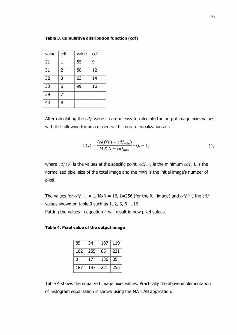
Table 3. Cumulative distribution function (cdf)
value cdf value cdf
21 1 55 9
31 2 58 12
32 3 63 14
33 6 99 16
39 7
43 8
After calculating the value it can be easy to calculate the output image pixel values
with the following formula of general histogram equalization as :
where is the values at the specific point, is the minimum , L is the
normalized pixel size of the total image and the MXN is the initial image‟s number of
pixel.
The values for = 1, MxN = 16, L=256 (for the full image) and the
values shown on table 3 such as 1, 2, 3, 6 … 16.
Putting the values in equation 4 will result in new pixel values.
Table 4. Pixel value of the output image
85 34 187 119
102 255 85 221
0 17 136 85
187 187 221 255
Table 4 shows the equalized image pixel values. Practically the above implementation
of histogram equalization is shown using the MATLAB application.
17
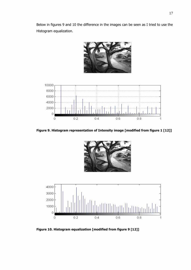
Below in figures 9 and 10 the difference in the images can be seen as I tried to use the
Histogram equalization.
Figure 9. Histogram representation of Intensity image [modified from figure 1 [12]]
Figure 10. Histogram equalization [modified from figure 9 [12]]
18
As can be seen from figures 9 and 10 the histogram equalization has caused figure 10
to have a better contrast with respect to the former image (figure 9). Also it shows the
intensities are well distributed on the histogram diagram.
3.2.3 Histogram Matching
The histogram matching method deals with the generation of a processed image that
has a specific histogram. Histogram matching can also be called histogram
specification. This method uses the following procedures:
a. First get the histogram of a given image
b. Then use some equation and pre-compute the mapping level s and r values
c. Compute each transformation functions and pre-compute the pixel values
d. Then map them to their final levels. [4]
There are certain difficulties while dealing with histogram matching to image
enhancement. In constructing a histogram either a particular probability function is
specified and the histogram is formed by digitizing the given function or a histogram
shape is specified on a graphic device and then is fed to the processor executing the
histogram specification algorithm.
3.3 Image Subtraction
Image subtraction deals with the difference between the pixel values of each function.
It can be represented by the equation
where g (x, y) is the final image obtained after the difference between all pairs of the
corresponding pixels of f (x, y) and h (x, y).
19
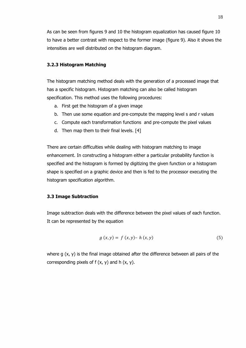
Figure 11. Intensity image [modified from figure 3 [12]]
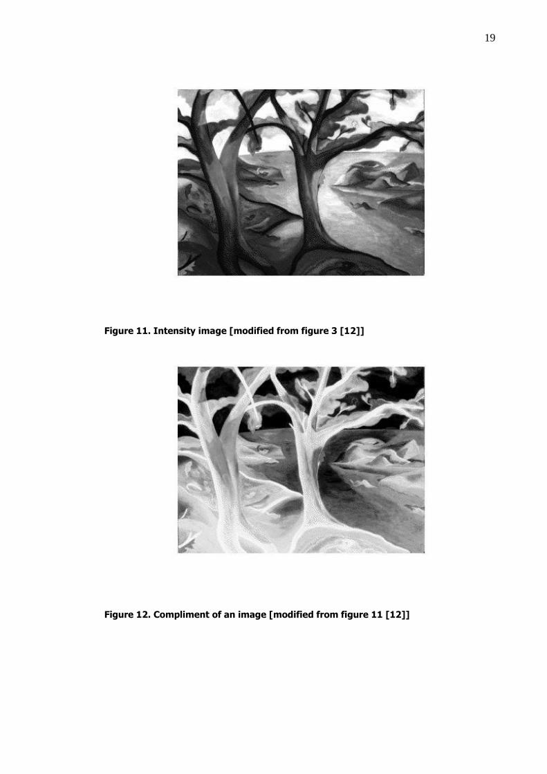
Figure 12. Compliment of an image [modified from figure 11 [12]]
20
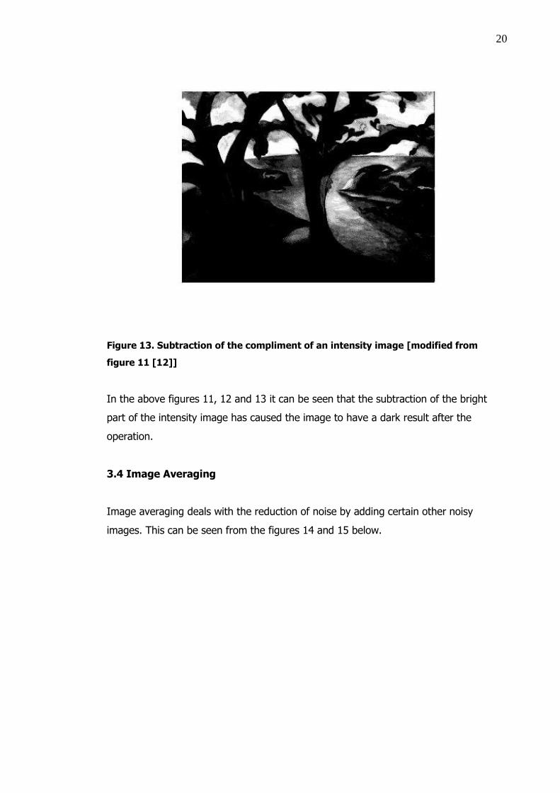
Figure 13. Subtraction of the compliment of an intensity image [modified from
figure 11 [12]]
In the above figures 11, 12 and 13 it can be seen that the subtraction of the bright
part of the intensity image has caused the image to have a dark result after the
operation.
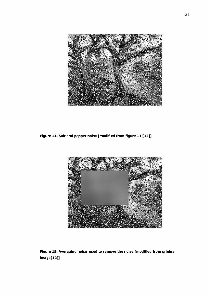
3.4 Image Averaging
Image averaging deals with the reduction of noise by adding certain other noisy
images. This can be seen from the figures 14 and 15 below.
21
Figure 14. Salt and pepper noise [modified from figure 11 [12]]
Figure 15. Averaging noise used to remove the noise [modified from original
image[12]]
22
In the figure 14 above a salt and pepper noise has been created on the intensity
image. Then averaging mask is used to remove the salt and pepper noise to have a
better image but the result has become a rather blurred image shown in figure 15 that
only remove the noise created.
3.5 Spatial Filtering
In spatial filtering a certain filter mask is used in all points in an image. The filter mask
is made of m x n size where the m and n are the matrix sizes. In each case the image
points should have the same matrix size as of the filter mask with size M x N.
There are two kinds of filtering, linear and non-linear spatial filtering. In low-pass filter
the attenuation of high frequencies from frequency domains causes in the blurring of
an image. While in high-pass filter the removal of low frequencies cause in the
sharpening of edges. Band-pass filtering is used for image restoration while removing
frequencies between high and low frequencies. There are many filters that are used for
blurring/smoothing, sharpening and edge detection in an image. These different
effects can be achieved by different coefficients in the mask.
3.6 Smoothing Spatial Filter
Smoothening filters can be obtained by averaging of pixels in the neighborhood of a
filter mask. It results in the blurring of an image. During noise removal or noise
reduction sharp edges are removed from the image. This will result in a blurred image.
Random noises have sharp transitions. While filtering those sharp transitions the edges
of an image which are important features of an image are lost. Averaging filters are
used also in smoothening of false contours.
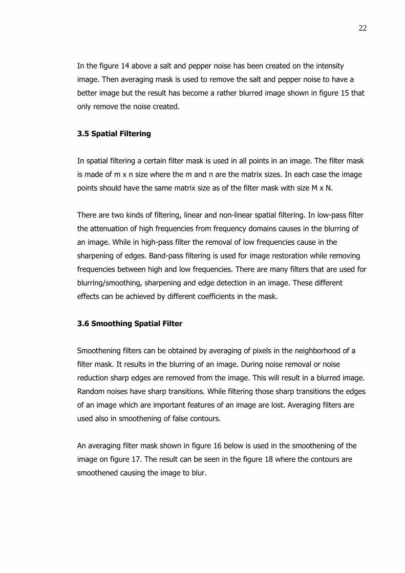
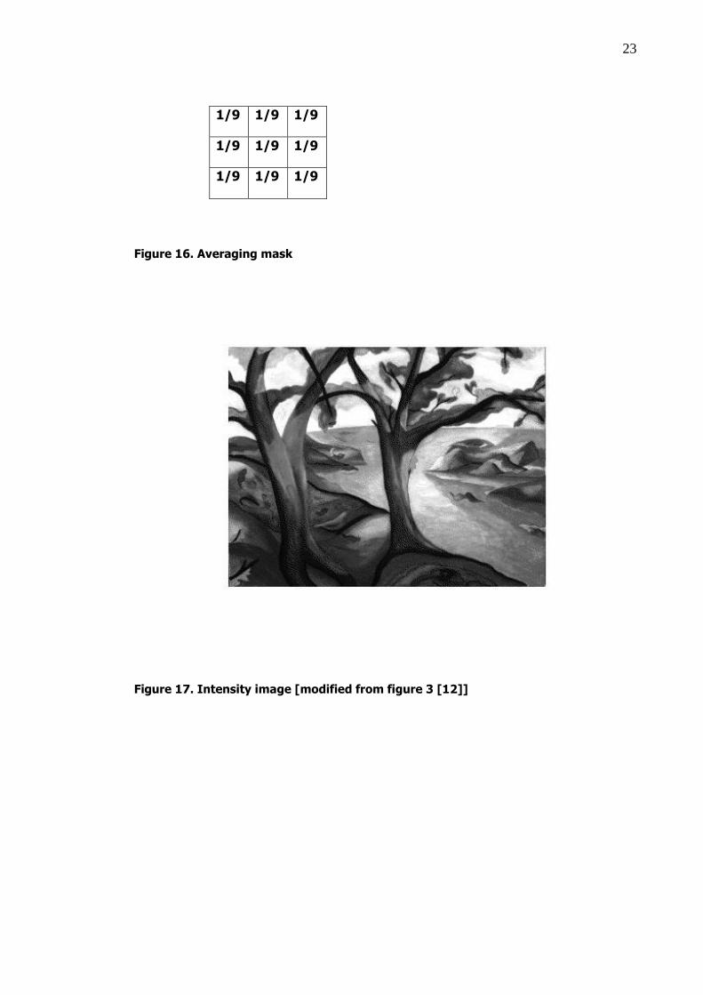
An averaging filter mask shown in figure 16 below is used in the smoothening of the
image on figure 17. The result can be seen in the figure 18 where the contours are
smoothened causing the image to blur.
23
1/9 1/9 1/9
1/9 1/9 1/9
1/9 1/9 1/9
Figure 16. Averaging mask
Figure 17. Intensity image [modified from figure 3 [12]]
24
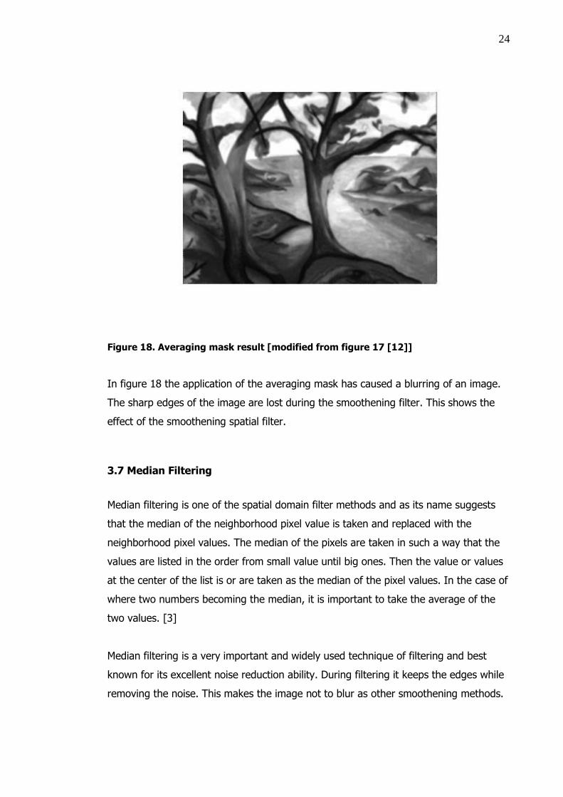
Figure 18. Averaging mask result [modified from figure 17 [12]]
In figure 18 the application of the averaging mask has caused a blurring of an image.
The sharp edges of the image are lost during the smoothening filter. This shows the
effect of the smoothening spatial filter.
3.7 Median Filtering
Median filtering is one of the spatial domain filter methods and as its name suggests
that the median of the neighborhood pixel value is taken and replaced with the
neighborhood pixel values. The median of the pixels are taken in such a way that the
values are listed in the order from small value until big ones. Then the value or values
at the center of the list is or are taken as the median of the pixel values. In the case of
where two numbers becoming the median, it is important to take the average of the
two values. [3]
Median filtering is a very important and widely used technique of filtering and best
known for its excellent noise reduction ability. During filtering it keeps the edges while
removing the noise. This makes the image not to blur as other smoothening methods.
25
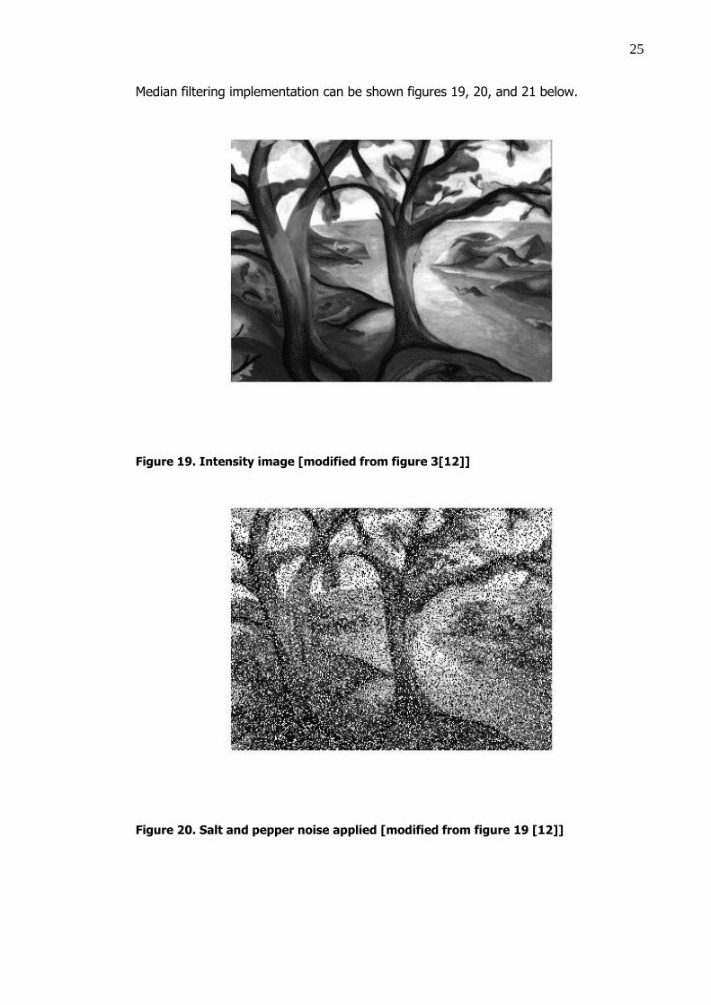
Median filtering implementation can be shown figures 19, 20, and 21 below.
Figure 19. Intensity image [modified from figure 3[12]]
Figure 20. Salt and pepper noise applied [modified from figure 19 [12]]
26
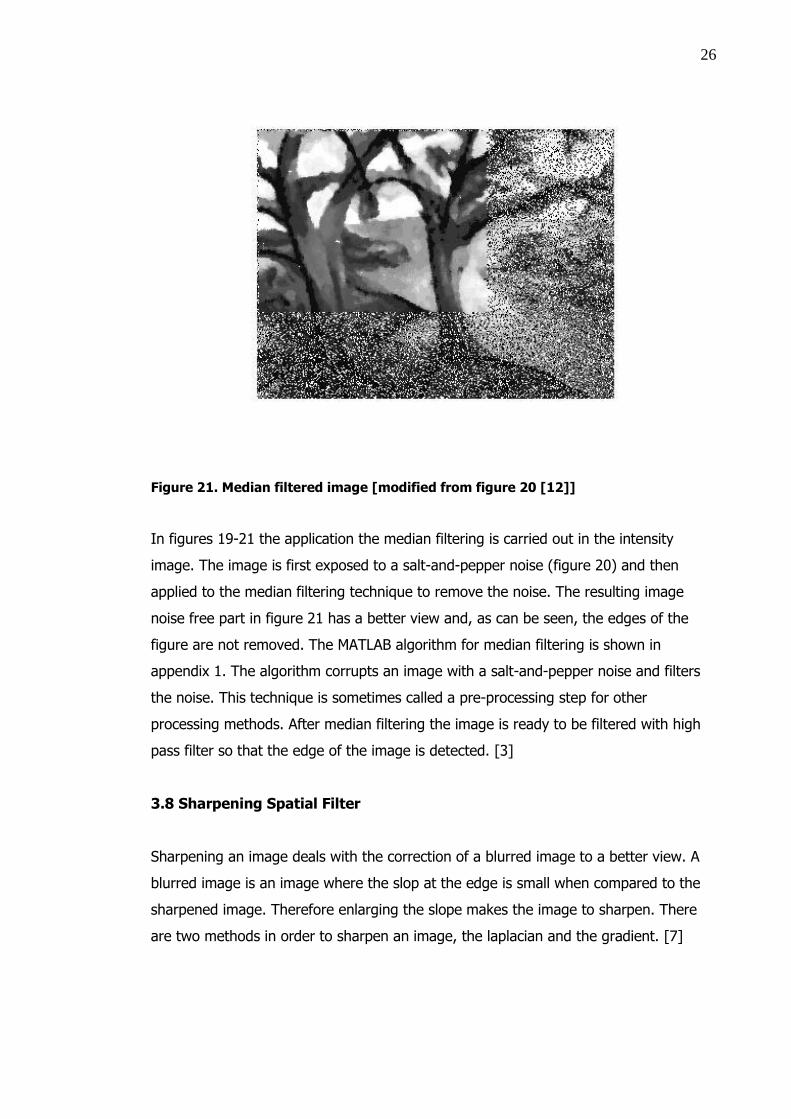
Figure 21. Median filtered image [modified from figure 20 [12]]
In figures 19-21 the application the median filtering is carried out in the intensity
image. The image is first exposed to a salt-and-pepper noise (figure 20) and then
applied to the median filtering technique to remove the noise. The resulting image
noise free part in figure 21 has a better view and, as can be seen, the edges of the
figure are not removed. The MATLAB algorithm for median filtering is shown in
appendix 1. The algorithm corrupts an image with a salt-and-pepper noise and filters
the noise. This technique is sometimes called a pre-processing step for other
processing methods. After median filtering the image is ready to be filtered with high
pass filter so that the edge of the image is detected. [3]
3.8 Sharpening Spatial Filter
Sharpening an image deals with the correction of a blurred image to a better view. A
blurred image is an image where the slop at the edge is small when compared to the
sharpened image. Therefore enlarging the slope makes the image to sharpen. There
are two methods in order to sharpen an image, the laplacian and the gradient. [7]
27
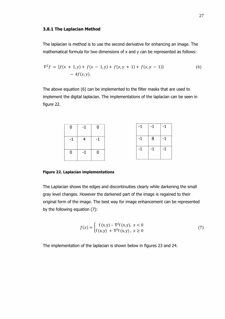
3.8.1 The Laplacian Method
The laplacian is method is to use the second derivative for enhancing an image. The
mathematical formula for two dimensions of x and y can be represented as follows:
The above equation (6) can be implemented to the filter masks that are used to
implement the digital laplacian. The implementations of the laplacian can be seen in
figure 22.
Figure 22. Laplacian implementations
The Laplacian shows the edges and discontinuities clearly while darkening the small
gray level changes. However the darkened part of the image is regained to their
original form of the image. The best way for image enhancement can be represented
by the following equation (7):
The implementation of the laplacian is shown below in figures 23 and 24.
0 -1 0
-1 4 -1
0 -1 0
-1 -1 -1
-1 8 -1
-1 -1 -1
28
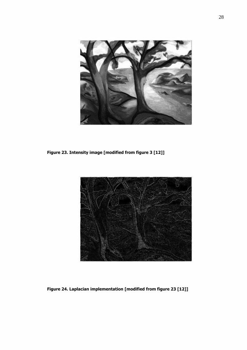
Figure 23. Intensity image [modified from figure 3 [12]]
Figure 24. Laplacian implementation [modified from figure 23 [12]]
29
The masks given in figure 22 are implemented on the intensity image in figure 23 to
result in a sharpened image in figure 24. Areas with high gray level changes can be
seen exposed while those with small gray level changes being dark and grayish. The
algorithm for spatial sharpening is shown in appendix 1. As can be seen, a sharpening
mask is used to filter an image.
3.8.2 The Gradient Method
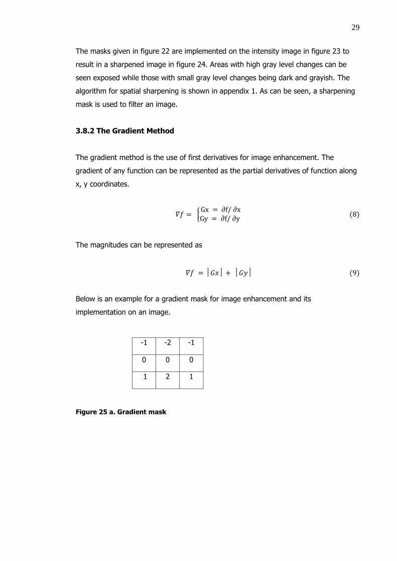
The gradient method is the use of first derivatives for image enhancement. The
gradient of any function can be represented as the partial derivatives of function along
x, y coordinates.
The magnitudes can be represented as
Below is an example for a gradient mask for image enhancement and its
implementation on an image.
Figure 25 a. Gradient mask
-1 -2 -1
0 0 0
1 2 1
30
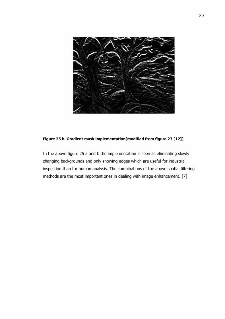
Figure 25 b. Gradient mask implementation[modified from figure 23 [12]]
In the above figure 25 a and b the implementation is seen as eliminating slowly
changing backgrounds and only showing edges which are useful for industrial
inspection than for human analysis. The combinations of the above spatial filtering
methods are the most important ones in dealing with image enhancement. [7]
31
4 Frequency Domain Image Enhancement
The image to be processed is transformed from spatial domain to frequency domain by
the Fourier transform. After the needed frequencies removed it is easy to return back
to the spatial domain.
4.1 Fourier Transform
The Fourier transform can be one dimensional or two dimensional depending on the
variables in the spatial domain. In image processing two-dimensional Fourier transform
is used. Before that it is good to define the Fourier transform. A Fourier transform is a
representation of non-periodic functions as an integral of sine and cosine functions. In
image processing the image is decomposed into sine and cosine components. Fourier
transforms for one dimension can be represented below in the form
The inverse can be represented as
The above formulas can be extended to two dimensions as
4.2 The Discrete Fourier Transform
The discrete Fourier transform has contained samples of the Fourier transform which
can describe the spatial domain image. In the discrete Fourier transform the sample
does not include all the frequencies of the image but rather a few samples. It can be
32
represented as one-dimensional or two-dimensional according to the variables. For
image processing the two-dimensional approach is
while the inverse is
where f(x, y) is M x N image, F (u, v) is the discrete Fourier transform of f(x, y).
The value of the transform is a complex number. Therefore to calculate the magnitude
of the spectrum the following formula is used.
Where I (u, v) and R (u, v) are the components of the complex transform.
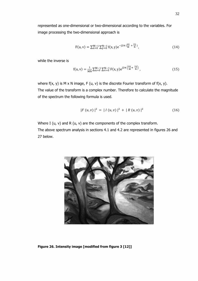
The above spectrum analysis in sections 4.1 and 4.2 are represented in figures 26 and
27 below.
Figure 26. Intensity image [modified from figure 3 [12]]
33
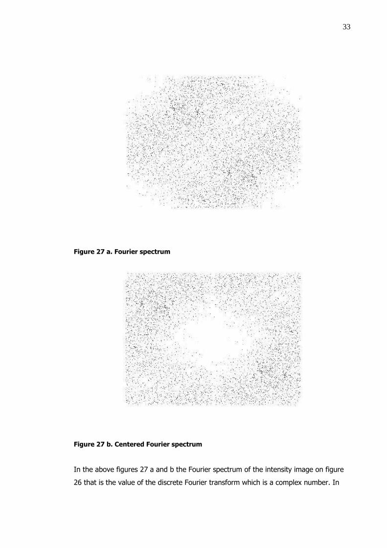
Figure 27 a. Fourier spectrum
Figure 27 b. Centered Fourier spectrum
In the above figures 27 a and b the Fourier spectrum of the intensity image on figure
26 that is the value of the discrete Fourier transform which is a complex number. In
34
the Centered Fourier transform the origin of the transform is shifted to the center of
the frequency.
4.3 Smoothing Frequency Domain Filter
In section 3.6 it is defined that smoothening is a attenuating a frequency frequencies
of a certain range. In the frequency domain the same is true. In order to attenuate the
frequency it is important to choose the right filtering function. Depending on the range
of smoothness there are different filter types. Among them are Ideal and Butterworth
low-pass filters. [3]
4.3.1 Ideal Low-pass Filter
An ideal low pass filter deals with the removal of all high frequency values of the
Fourier transform out of the range of a specified distance. There is a general formula
for filtering that is
where the H (u, v) is the transfer function, and F (u, v) is the Fourier transform of the
image function. The G (u, v) is the filtered final function. In all the filters it is important
to find the right filter function to deal with. The right filter for the Ideal low-pass filter
is given by
where the is a defined non negative and D (u, v) is the distance from the center of
the frequency to the point (u, v). In the tree picture that I am dealing with it, the ideal
low pass filter can be seen as follows:

35
Figure 28. Intensity image [modified from figure 3 [12]]
Figure 29. Smoothened image [modified from figure 28[12]]
36
Figure 30. Logarithmically scaled amplitude spectrum
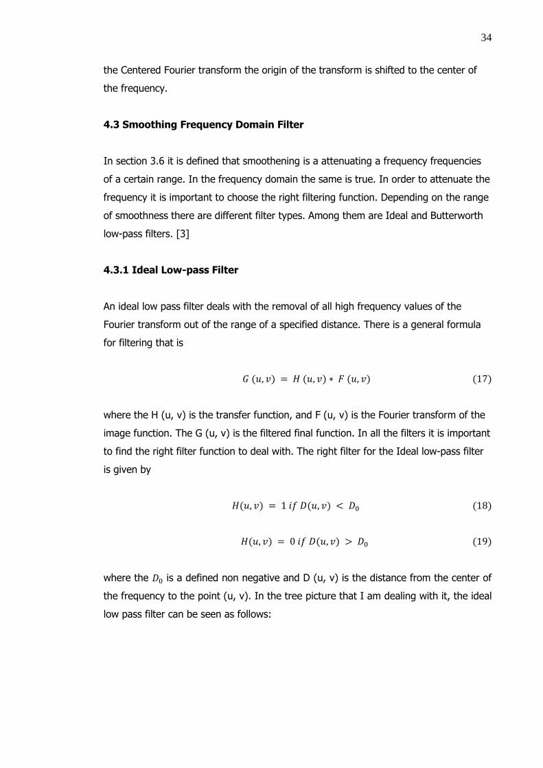
Figure 31. Idealized low-pass image as an amplitude spectrum of image
37
In figures 28, 29, 30 and 31 the tree picture is ideally low-pass filtered with the
transfer function as discussed in section 4.3.1. This transfer function action can be
seen in figure 31 where other out of the radius of 10 equal to zero. It is possible to
change the size of the radius depending on how the user wants to filter. In figure 31
the amplitude spectrum of the idealized low-pass filtered of the tree image is shown.
The horizontal scale representing the largest matrix dimension of the image. For
example if the matrix dimension of an image is 258x350, then the horizontal scale is
from 0 to 349. The MATLAB algorithm is shown for ideal low pass filter in appendix 2.
In the algorithm an image is corrupted with a noise and filtered with the ideal low pass
filter.
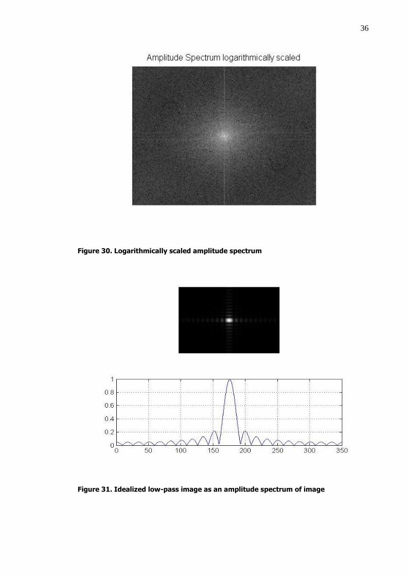
4.3.2 Butterworth Low-pass Filter
In the Butterworth low-pass filter the transfer function is different:
where D (u, v) is the distance from any point (u, v) to the center of the origin of the
Fourier transform. [2] The Butterworth low-pass filter can be seen in figure 32 below.
The MATLAB algorithm for Butterworth low pass filter is shown in appendix 2. The
algorithm uses the Butterworth low pass filter formula directly and filters an image.
38
Figure 32. Butterworth low-pass represented as an image
Figure 32 shows that the spatial representation of the Butterworth low-pass filter. As
the order of the filter increases, the ringing effect increases. In figure 32 the cutoff
frequency distance from the origin is equal to 4. The horizontal scale represents the
matrix dimension of the tree picture.
4.4 Sharpening in Frequency Domain
Edges and high frequency changes in an image are the basic parts. Most of the time
they are associated with the high frequency values. In order to deal with them we filter
out all the low frequency components with no change at the high ones. Therefore the
process to attenuate the low frequencies is called high-pass filtering. In high-pass
filtering an image is sharpened. High-pass filtering can be represented by the following
equation:
where the high-pass is transfer function and is the low-pass transfer
function.
39
4.4.1 Ideal High-pass Filter
The ideal high pass filter is the exact opposite of ideal low-pass filter with the transfer
function
where is a cutoff frequency from the origin and D (u, v) is the distance from any
point (u, v) to the center of the origin of the Fourier transform. [10]
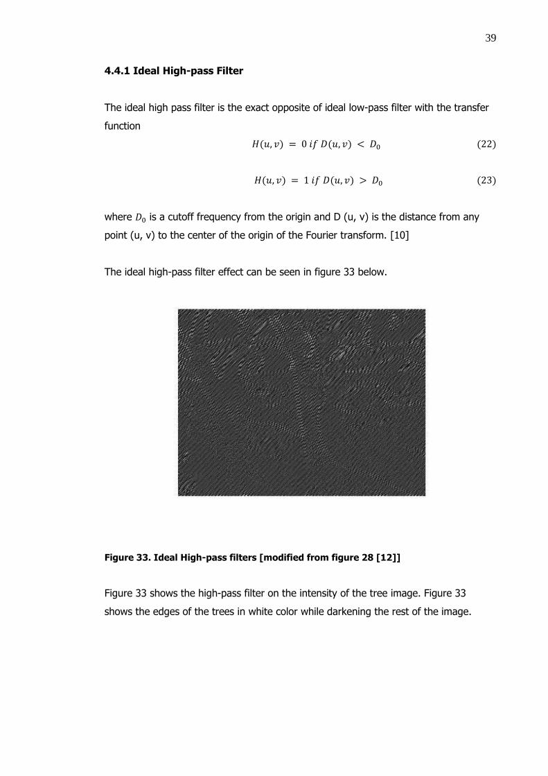
The ideal high-pass filter effect can be seen in figure 33 below.
Figure 33. Ideal High-pass filters [modified from figure 28 [12]]
Figure 33 shows the high-pass filter on the intensity of the tree image. Figure 33
shows the edges of the trees in white color while darkening the rest of the image.
40
4.4.2 Butterworth High-pass Filter
The Butterworth high-pass filter has a transfer function of
where D (u, v) is the distance from any point (u, v) to the center of the origin of the
Fourier transform and is the cutoff frequency from the origin. [3]
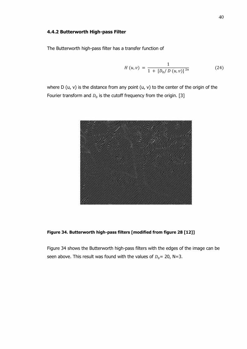
Figure 34. Butterworth high-pass filters [modified from figure 28 [12]]
Figure 34 shows the Butterworth high-pass filters with the edges of the image can be
seen above. This result was found with the values of = 20, N=3.
41
5 Image Restoration
An image is restored after it has lost its most important features or degraded. An
image could be degraded during digitization or during transmission. During digitization
or transmission a noise may be included in a digital image from the environment
around it. For example, while taking a picture using a camera a noise is added by the
camera fault, the image sensor or from the environment where the image is taken.
When it is from the camera fault it means if the shutter speed of the camera is too
long. This causes a noise type called salt-and-pepper. Image sensors are made to
collect light. During collection of light more light might be collected and causes high
temperature which would result in Gaussian noise type. But when it is from the
environment where the image is taken it might be from light reflections.
During image transmission the noise might be caused by a small bandwidth which
causes the image not to transmit fully making it blur. A noise is caused by the
environment around us. [4] Therefore it is important to restore the images to their
original features by removing the noise. In order to remove the noise someone has to
know the noise itself so that it would be easy to remove it. Different types of noises
are studied by adding them to an original image and use certain ways to remove those
noises.
5.1 Noise Types
For an image to be restored it is important to know the features of the noises that
caused its degradation. They have different features but the most important in this
project are the spatial and frequency properties. Spatial properties mean dealing with
the statistical behaviors of the noise component, while in frequency properties deal
with the frequency contents of the noise in Fourier form. [3]
There are many noise patterns in image processing and some of them include: [3]
a) Gaussian noise – is a noise type initiated by a Gaussian amplitude distribution.
The Gaussian probability distribution has a a probability density function of
42
where x is the gray level is the mean, the standard deviation and the
variance.
b) Erlang (Gamma) noise – is a noise having a probability distribution function of
where the mean is
and variance
. The parameters a and b are
positive integers and “ ” is factorial.
c) exponential noise – is a noise with exponential probability density function of
where the mean
and
for a>0.
d) uniform noise – is the noise with the probability density function of
where the mean is
and variance is
.
e) impulse noise(salt-and-pepper) – is a noise type with a probability density
function of
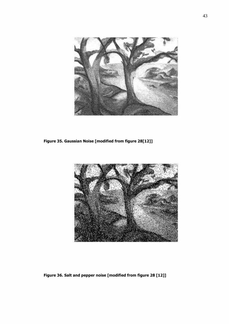
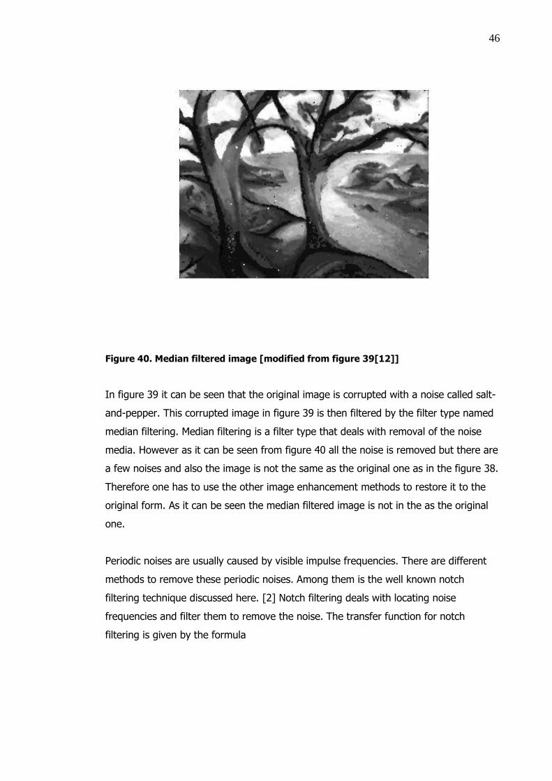
Applying some of the noises to the tree image can be shown in figures 35, 36, 37.
43
Figure 35. Gaussian Noise [modified from figure 28[12]]
Figure 36. Salt and pepper noise [modified from figure 28 [12]]

44
Figure 37. Uniform noise [modified from figure 28 [12]]
In the above figures 35, 36 and 37 the tree images that I am dealing with is changed
to intensity image and added noise. The noises added are of different types. In order
to restore the image to its original noise-free image, it is important to know the
features of the noises themselves.
5.2 Noise Filtering in Spatial and Frequency Domain
Noise filtering techniques were discussed in sections 3.6-3.8 and 4.3-4.4. Here I
discuss only new methods for filtering in the spatial and frequency. A salt-and-pepper
noise applied to the image has resulted in an image in figure 36. Using the median
filtering technique caused the noise to be removed. This can be seen in image
illustrations on figures 38, 39 and 40.

45
Figure 38. Intensity image [modified from figure 3 [12]]
Figure 39. Salt and pepper noise [modified from figure 38 [12]]
46
Figure 40. Median filtered image [modified from figure 39[12]]
In figure 39 it can be seen that the original image is corrupted with a noise called salt-
and-pepper. This corrupted image in figure 39 is then filtered by the filter type named
median filtering. Median filtering is a filter type that deals with removal of the noise
media. However as it can be seen from figure 40 all the noise is removed but there are
a few noises and also the image is not the same as the original one as in the figure 38.
Therefore one has to use the other image enhancement methods to restore it to the
original form. As it can be seen the median filtered image is not in the as the original
one.
Periodic noises are usually caused by visible impulse frequencies. There are different
methods to remove these periodic noises. Among them is the well known notch
filtering technique discussed here. [2] Notch filtering deals with locating noise
frequencies and filter them to remove the noise. The transfer function for notch
filtering is given by the formula
47
where
and
where n is the order. Also ( , ) and ( , ) are the center of the notches and
is the radius. M and N are the rows and columns respectively. The application for the
notch filtering in the tree image that I am dealing with can be seen in figures 41-44.
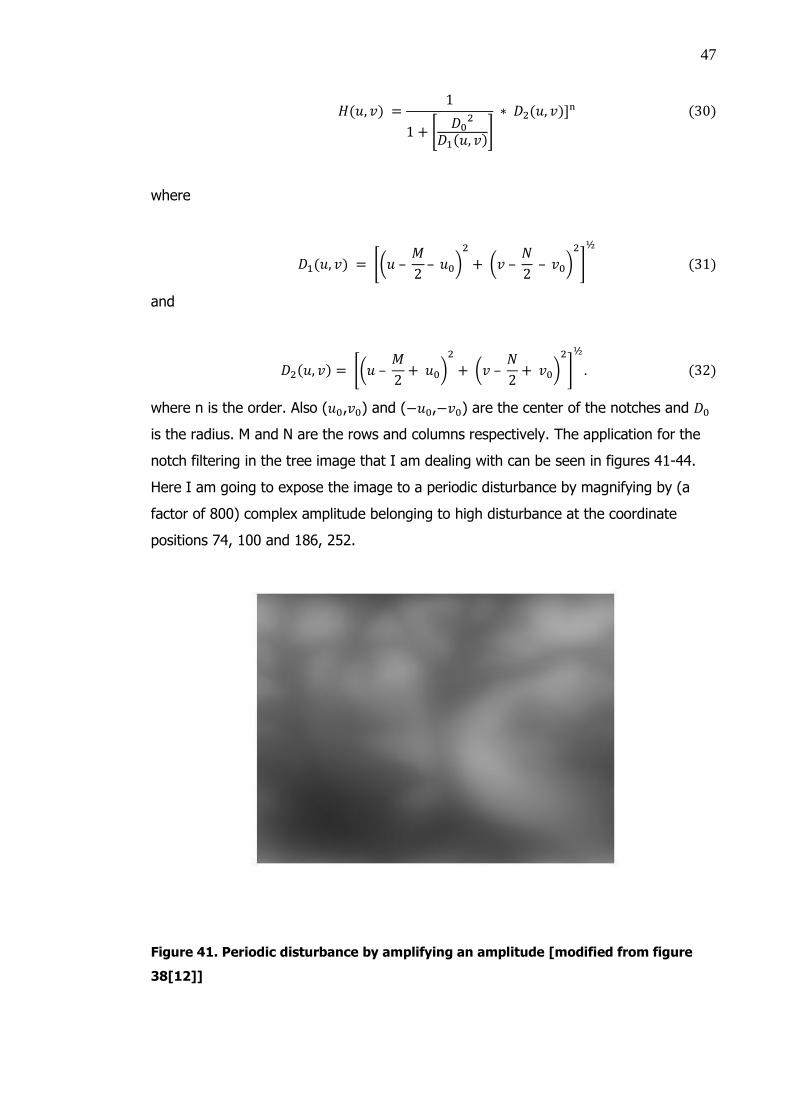
Here I am going to expose the image to a periodic disturbance by magnifying by (a
factor of 800) complex amplitude belonging to high disturbance at the coordinate
positions 74, 100 and 186, 252.
Figure 41. Periodic disturbance by amplifying an amplitude [modified from figure
38[12]]
48
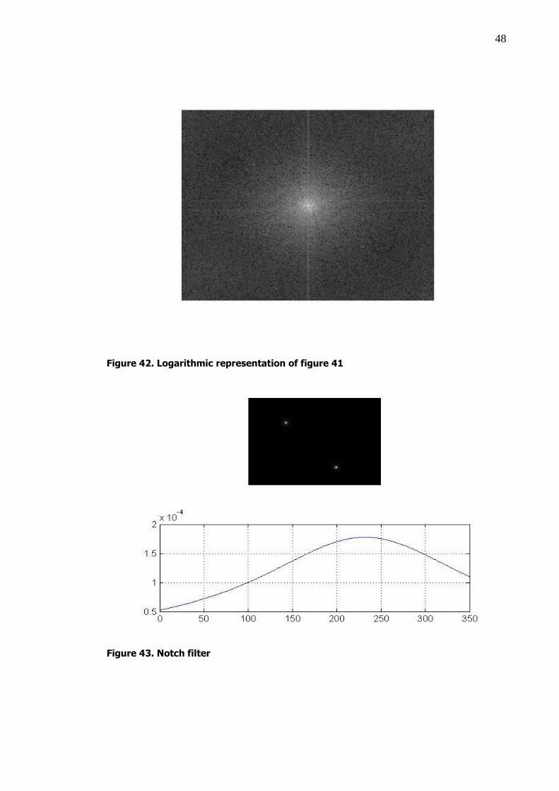
Figure 42. Logarithmic representation of figure 41
Figure 43. Notch filter
49
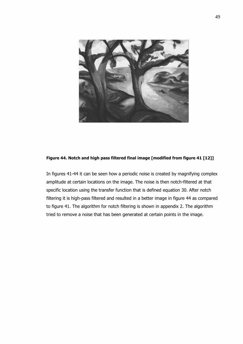
Figure 44. Notch and high pass filtered final image [modified from figure 41 [12]]
In figures 41-44 it can be seen how a periodic noise is created by magnifying complex
amplitude at certain locations on the image. The noise is then notch-filtered at that
specific location using the transfer function that is defined equation 30. After notch
filtering it is high-pass filtered and resulted in a better image in figure 44 as compared
to figure 41. The algorithm for notch filtering is shown in appendix 2. The algorithm
tried to remove a noise that has been generated at certain points in the image.
50
6. Analysis of Spatial and Frequency Methods and Results
In chapters 3, 4 and 5 I tried to explain the methods used to filter noise, enhancing
contrast and sharpening digital image. Noise filtering is carried out by spatial and
frequency low-pass filtering, Contrast enhancement is carried out with spatial domain
histogram stretching and sharpening of an image uses the spatial and frequency
domain high-pass filtering. The results of the methodologies will be discussed here.
6.1 Analysis of Spatial Image Filtering
In spatial image filtering the noise reduction, image sharpening and contrast
enhancement are performed by manipulating the pixels values using certain masks
applied on the image. For Noise reduction the masks used are smoothening masks, like
the one on figure 15. In figure 15 the image is noise free but the resulting image is
blurred. So in order to correct it, sharpening mask is used in order to sharpen the
edges of the image. However edge sharpening is not the only method that is used. The
power-law method is used in order to enhance the contrast by using some gamma
correction values. From the above discussion it can be seen that image enhancement
in the spatial domain is only done by manipulating the pixels.
6.2 Analysis of the Frequency Domain
In the frequency domain the image enhancement deals with the frequency values
manipulation. In the frequency domain the high or low frequencies are cut off
depending on the result needed. In this method a low-pass filter is used in order to
remove noise. After removing the noise the image becomes blurred as in the same
case as the spatial ones as shown in section 3.7. Therefore it is important to sharpen it
using high pass filter to deal with the edges. In the frequency domain filtering, similar
to the spatial domain filtering there are different methods to like the Butterworth low-
pass and high-pass filters, ideal low pass and high-pass and so forth.
51
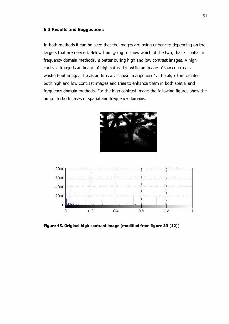
6.3 Results and Suggestions
In both methods it can be seen that the images are being enhanced depending on the
targets that are needed. Below I am going to show which of the two, that is spatial or
frequency domain methods, is better during high and low contrast images. A high
contrast image is an image of high saturation while an image of low contrast is
washed-out image. The algorithms are shown in appendix 1. The algorithm creates
both high and low contrast images and tries to enhance them in both spatial and
frequency domain methods. For the high contrast image the following figures show the
output in both cases of spatial and frequency domains.
Figure 45. Original high contrast image [modified from figure 39 [12]]
52
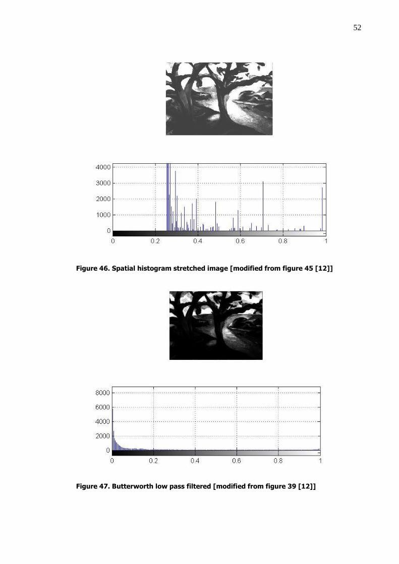
Figure 46. Spatial histogram stretched image [modified from figure 45 [12]]
Figure 47. Butterworth low pass filtered [modified from figure 39 [12]]
53
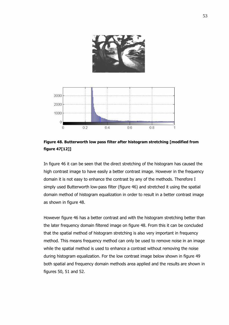
Figure 48. Butterworth low pass filter after histogram stretching [modified from
figure 47[12]]
In figure 46 it can be seen that the direct stretching of the histogram has caused the
high contrast image to have easily a better contrast image. However in the frequency
domain it is not easy to enhance the contrast by any of the methods. Therefore I
simply used Butterworth low-pass filter (figure 46) and stretched it using the spatial
domain method of histogram equalization in order to result in a better contrast image
as shown in figure 48.
However figure 46 has a better contrast and with the histogram stretching better than
the later frequency domain filtered image on figure 48. From this it can be concluded
that the spatial method of histogram stretching is also very important in frequency
method. This means frequency method can only be used to remove noise in an image
while the spatial method is used to enhance a contrast without removing the noise
during histogram equalization. For the low contrast image below shown in figure 49
both spatial and frequency domain methods area applied and the results are shown in
figures 50, 51 and 52.
54
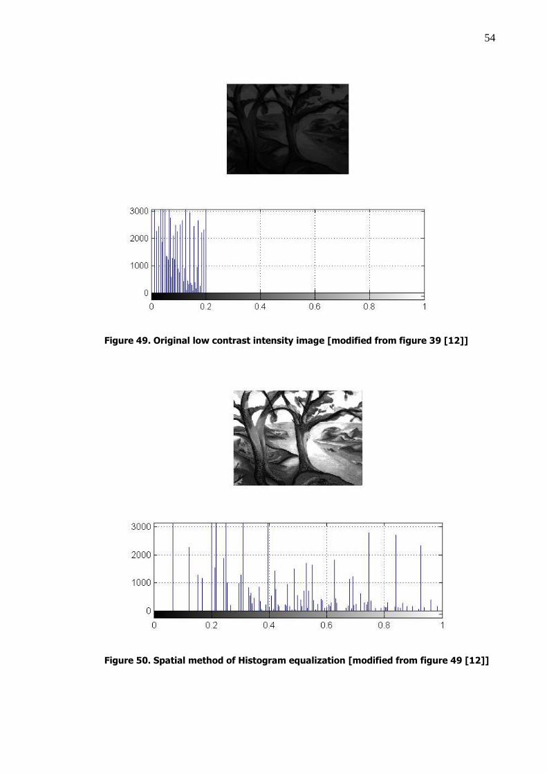
Figure 49. Original low contrast intensity image [modified from figure 39 [12]]
Figure 50. Spatial method of Histogram equalization [modified from figure 49 [12]]
55
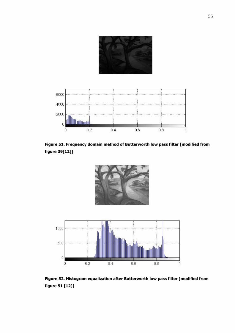
Figure 51. Frequency domain method of Butterworth low pass filter [modified from
figure 39[12]]
Figure 52. Histogram equalization after Butterworth low pass filter [modified from
figure 51 [12]]
56
In figures 49, 50, 51 and 52 it can be seen similar advantage of the spatial domain
histogram equalization method is applicable. In figure 50 the direct application of
spatial domain histogram equalization resulted in a well-balanced image of good
contrast. Also in figure 52 the application of the Butterworth low-pass filter, figure 51,
is well improved by the spatial domain method of histogram equalization.
From the above examples, shown in figures 45-52, of high and low contrast images it
can be seen that both methods support each other to result in a better quality image.
Also the direct application of the spatial method of histogram equalization will make it
a better method in a quick response to the high or low contrast images. However it can
also be used in either way.
The advantage of the frequency domain method is that it can easily be used and the
parameters are easily manipulated even though it is not simple to smoothly distribute
the gray tones. For the smooth distribution of the gray tones, as the above examples
in figures 45-52 have suggested, the spatial domain method is the best method.
There are disadvantages in both methods. For the frequency domain ones that they
are good for removal of noises while that spatial ones are good for enhancing
contrasts. However the combinations of the two domains methodologies will result in
an image with a noise free sharp image in a very good contrast.
This project has tried to show the methods and algorithms applied to process an
image. However it is important to study the importance of these methods in other
image processing applications.
The advantages and disadvantages of the spatial and frequency methods are
summarized in table 5.
57
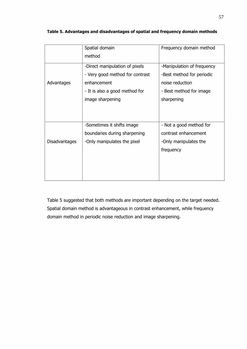
Table 5. Advantages and disadvantages of spatial and frequency domain methods
Spatial domain
method
Frequency domain method
Advantages
-Direct manipulation of pixels
- Very good method for contrast
enhancement
- It is also a good method for
image sharpening
-Manipulation of frequency
-Best method for periodic
noise reduction
- Best method for image
sharpening
Disadvantages
-Sometimes it shifts image
boundaries during sharpening
-Only manipulates the pixel
- Not a good method for
contrast enhancement
-Only manipulates the
frequency
Table 5 suggested that both methods are important depending on the target needed.
Spatial domain method is advantageous in contrast enhancement, while frequency
domain method in periodic noise reduction and image sharpening.
58
7 Conclusion
This paper tried to show the methods and importance of image processing. Image
processing is important in our daily lives and was discussed in section 2.1 that image
processing means any action in order to change an image. One of the image
processing techniques, the digital image processing, was discussed and in the methods
on how to apply were briefly explained. Digital image processing is an important field
that is used in different scientific researches and technology developments.
In this paper different domains were used with each its own methods to processes an
image. The domains discussed were the spatial and frequency domains. The
differences among the domains and their different methodologies were briefly
explained.
Generally the methods are both important and applicable in different technologies. In
this paper I tried to show a comparison between both approaches and tried to show
their advantages and disadvantages. This paper suggests that more researches is
needed on many other image processing applications to show the importance of those
methods.
59
References
1. The Math Works, Inc. [online].Pixel representation; 1984-2011.
URL: http://www.mathworks.com/help/toolbox/images/brcu_al-1.html
Accessed January 2011.
2. Rafael C. Gonzalez, Richard E. Woods, Steven L. Eddins Digital. Digital image
processing using MATLAB: Coordinate Conventions:
3. Rafael C. Gonzalez, Richard E. Woods. Digital image processing. Second edition
upper saddle River, NJ : Prentice Hall; 2002.
4. Gregory A. Baxes. Digital Image Processing Principles and Applications. John Wiley
& Sons, Inc; 1994.
5. Arash Abadpour. Color Image Processing Using Principal Component Analysis.
Tehran Iran, SHARIF University of Technology ; 2005.
6. Ming Zhang . Bilateral Filter Image Processing. Louisiana State University; 2009
7. W.H. Freeman. Digital image processing. New York.
URL:http://www.ciesin.org/docs/005-477/005-477.html . Accessed January 2011.
8. Robyn Owens. Frequency Domain Methods; October 1997.
URL:http://homepages.inf.ed.ac.uk/rbf/CVonline/LOCAL_COPIES/OWENS/LECT5/n
ode4.html. Accessed January 2011.
9. Jerry Lordriguss. Digital image processing;1974-2010.
URL: http://www.astropix.com/HTML/J_DIGIT/TOC_DIG.HTM . Accessed January
2011.
60
10. P.C Rossin. Image processing in frequency Domain. Lehigh University.
URL: http://www.cse.lehigh.edu/~spletzer/rip_f06/lectures/lec012_Frequency.pdf.
Accessed January 2011
11. Andrew Ghigo. The Contrast ratio game; March 9, 2011.
URL: http://www.practical-home-theater-guide.com/contrast-ratio.html. Accessed
April, 2011.
12. Trees image; copyright Susan Cohen; The Math Works, Inc. MATLAB software;
1984-2010.
61
Appendices
Appendix 1
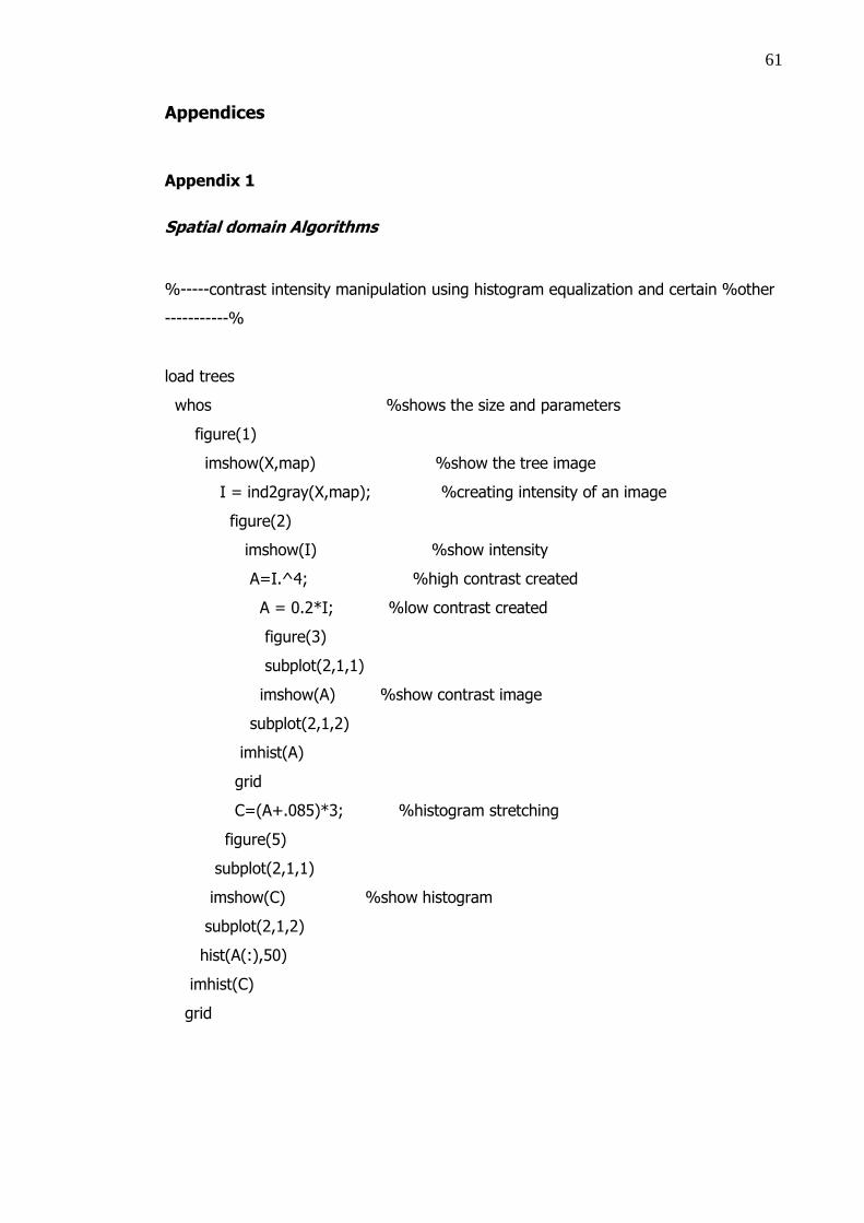
Spatial domain Algorithms
%-----contrast intensity manipulation using histogram equalization and certain %other
-----------%
load trees
whos %shows the size and parameters
figure(1)
imshow(X,map) %show the tree image
I = ind2gray(X,map); %creating intensity of an image
figure(2)
imshow(I) %show intensity
A=I.^4; %high contrast created
A = 0.2*I; %low contrast created
figure(3)
subplot(2,1,1)
imshow(A) %show contrast image
subplot(2,1,2)
imhist(A)
grid
C=(A+.085)*3; %histogram stretching
figure(5)
subplot(2,1,1)
imshow(C) %show histogram
subplot(2,1,2)
hist(A(:),50)
imhist(C)
grid
62
%-----------------------pixel manipulation with high pass filter mask--------------%
load trees
whos
figure(1)
imshow(X,map) % Indexed image
I=ind2gray(X,map); % Converting indexed image to intensity image
figure(2)
imshow(I) % Intensity image
%My=ones(3,3)/9; %averaging mask
My=zeros(3,3);
My(1,1)=-1;
My(1,2)=-1;
My(1,3)=-1 ;
My(2,1)=-1;
My(2,2)=8;
My(2,3)=-1 ;
My(3,1)=-1;
My(3,2)=-1;
My(3,3)=-1;
M=My; %the mask „My‟ can be changed depending on the result needed
FI=I; % Intiating the output matrix
for i=2:257
for j=2:349
FI(i,j)=sum(sum(I(i-1:i+1,j-1:j+1).*M)); %filtering with the mask
end
end
figure(4)
imshow(FI)
63
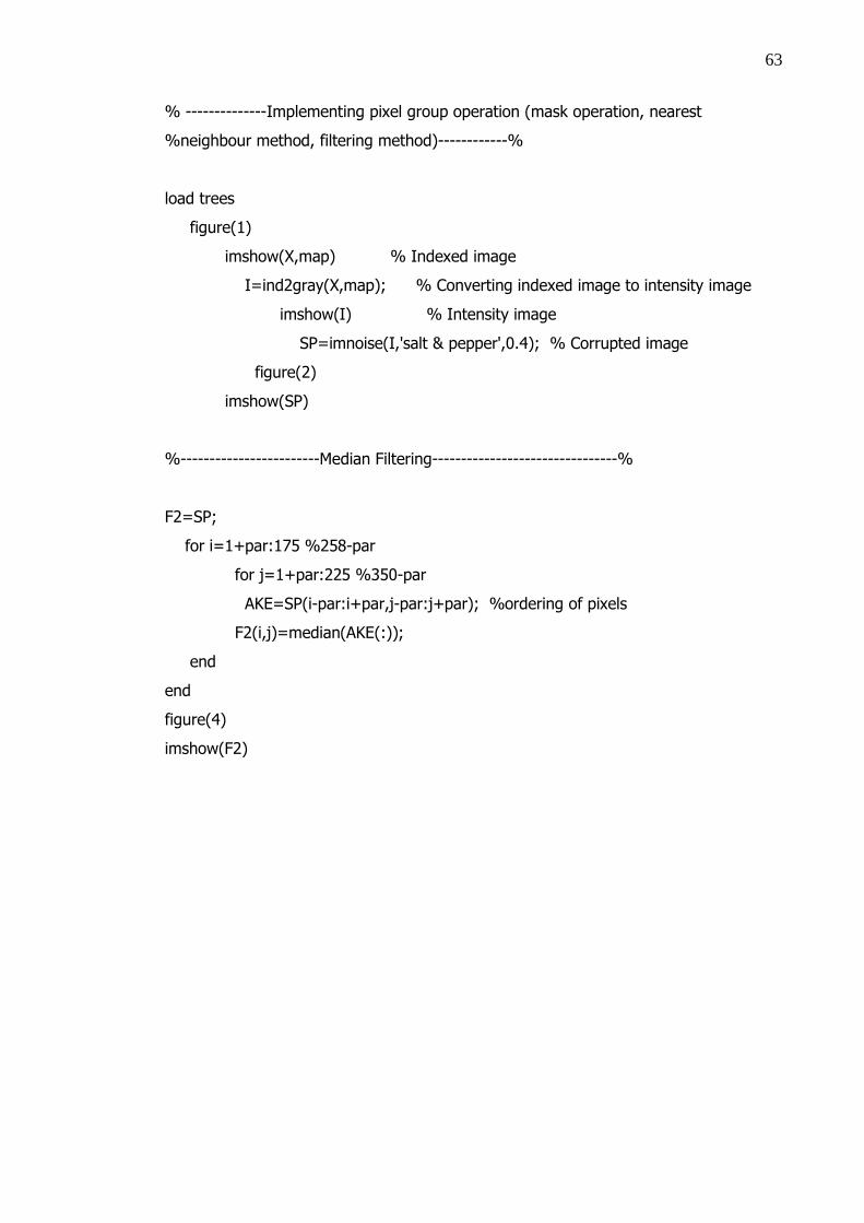
% --------------Implementing pixel group operation (mask operation, nearest
%neighbour method, filtering method)------------%
load trees
figure(1)
imshow(X,map) % Indexed image
I=ind2gray(X,map); % Converting indexed image to intensity image
imshow(I) % Intensity image
SP=imnoise(I,'salt & pepper',0.4); % Corrupted image
figure(2)
imshow(SP)
%------------------------Median Filtering--------------------------------%
F2=SP;
for i=1+par:175 %258-par
for j=1+par:225 %350-par
AKE=SP(i-par:i+par,j-par:j+par); %ordering of pixels
F2(i,j)=median(AKE(:));
end
end
figure(4)
imshow(F2)
64
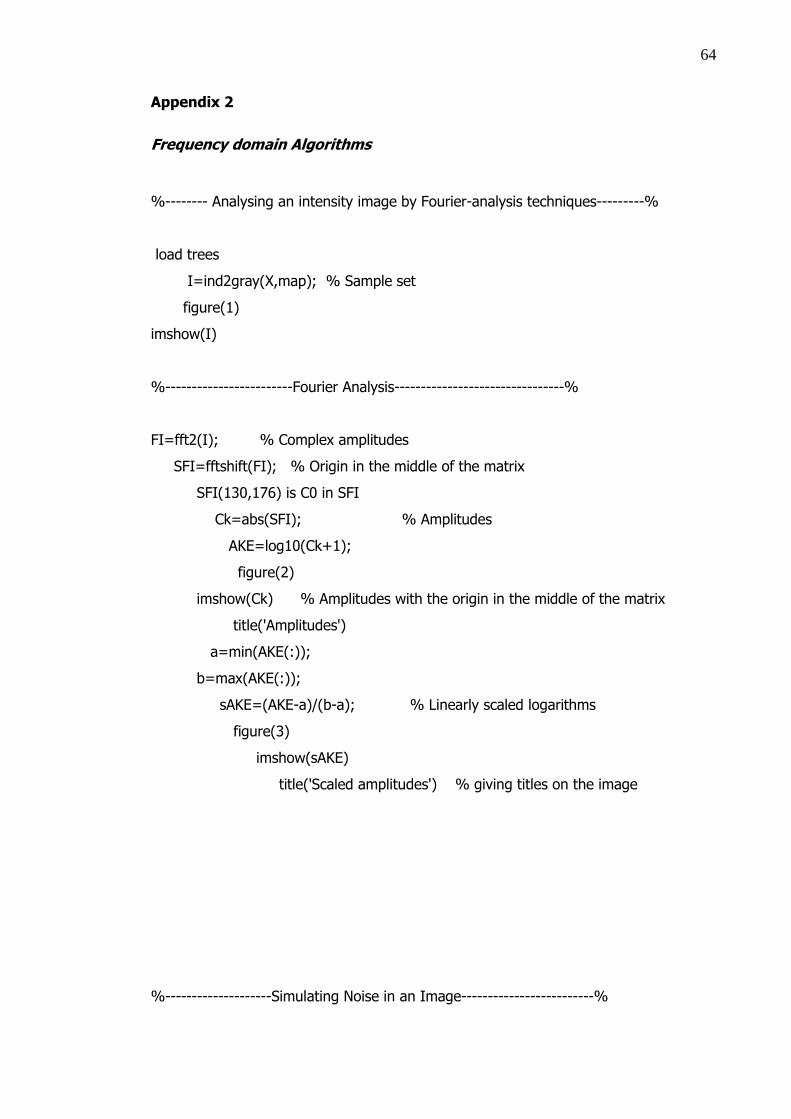
Appendix 2
Frequency domain Algorithms
%-------- Analysing an intensity image by Fourier-analysis techniques---------%
load trees
I=ind2gray(X,map); % Sample set
figure(1)
imshow(I)
%------------------------Fourier Analysis--------------------------------%
FI=fft2(I); % Complex amplitudes
SFI=fftshift(FI); % Origin in the middle of the matrix
SFI(130,176) is C0 in SFI
Ck=abs(SFI); % Amplitudes
AKE=log10(Ck+1);
figure(2)
imshow(Ck) % Amplitudes with the origin in the middle of the matrix
title('Amplitudes')
a=min(AKE(:));
b=max(AKE(:));
sAKE=(AKE-a)/(b-a); % Linearly scaled logarithms
figure(3)
imshow(sAKE)
title('Scaled amplitudes') % giving titles on the image
%--------------------Simulating Noise in an Image-------------------------%
65
MAT=SFI;
MAT(74,100)=800*MAT(74,100); %noise at the given coordinates
MAT(186,252)=800*MAT(186,252); %noise at the given coordinates
Ck=abs(MAT); % Amplitudes
AKE=log10(Ck+1);
a=min(AKE(:))
b=max(AKE(:))
sAKE=(AKE-a)/(b-a); % Linearly scaled logarithms
figure(4)
imshow(sAKE)
title('Scaled amplitudes')
IMG=ifft2(MAT);
figure(5)
imshow(abs(IMG))
%---------------------Ideal Low Pass Filter-------------------------------%
[m,n]=size(I);
M=zeros(m,n); % Initiating the low pass mask
M(130-par:130+par,176-par:176+par)=1;
fMAT=MAT.*M; % Filtering MAT
IMG2=ifft2(fMAT);
figure(6)
imshow(abs(IMG2))
%--------------Mask as an Amplitude Spectrum of an Image----------------%
figure(7) % Amplitude spectrum in frequency domain
subplot(2,1,1)
imshow(M)
subplot(2,1,2)
plot(M(130,:))
grid
66
IMG3=fftshift(ifft2(M));
figure(8)
aIMG3=abs(IMG3);
a3=min(aIMG3(:));
b3=max(aIMG3(:));
sIMG3=(aIMG3-a3)/(b3-a3); % enhancing the image with max. and min.values
% while removing the rest of the frequency values
%----------------------Butterworth Low Pass Filter---------------------------%
[V,U]=meshgrid(-175:174,-129:128);
D=sqrt(U.^2+V.^2);
H=1./(1+(D/D0).^(2*N)); % Butterworth Low Pass Filter
figure(9) % Amplitude spectrum in frequency domain
subplot(2,1,1)
imshow(H)
subplot(2,1,2)
plot(H(130,:))
grid
%------------------------------Notch Filter----------------------------------%
D1=sqrt((U+56).^2+(V+76).^2);
D2=sqrt((U-56).^2+(V-76).^2);
H1=1./(1+(D1/D0).^(2*N)); %implementing the notch filter formula
H2=1./(1+(D2/D0).^(2*N)); %implementing the notch filter formula
figure(9)
imshow(D2/max(D2(:)))
Hlow=H1+H2; % Local low pass filter in pole positions
High=1-Hlow;
figure(10)
imshow(High)