Embed Size (px)
Citation preview
Digital Image processing
Chapter 10
Image segmentation
By Lital Badash and Rostislav Pinski
Oct. 2010

2
Introduction
Mathematical background
Detection of isolated point
Line detection
Edge Models
Basic edge detection
Advanced edge detection
Edge linking and Boundary detection
Outline
3
Preview
Segmentation is to subdivide an image into its
component regions or objects.
Segmentation should stop when the objects of
interest in an application have been isolated.
4
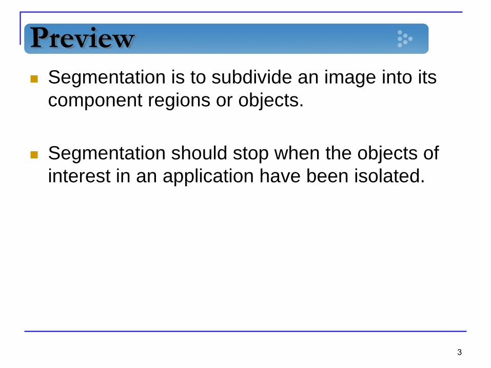
Preview - Example
5
Principal approaches
Segmentation algorithms generally are based on
one of 2 basis properties of intensity values:
discontinuity : to partition an image based on sharp
changes in intensity
similarity : to partition an image into regions that
are similar according to a set of predefined criteria.
6
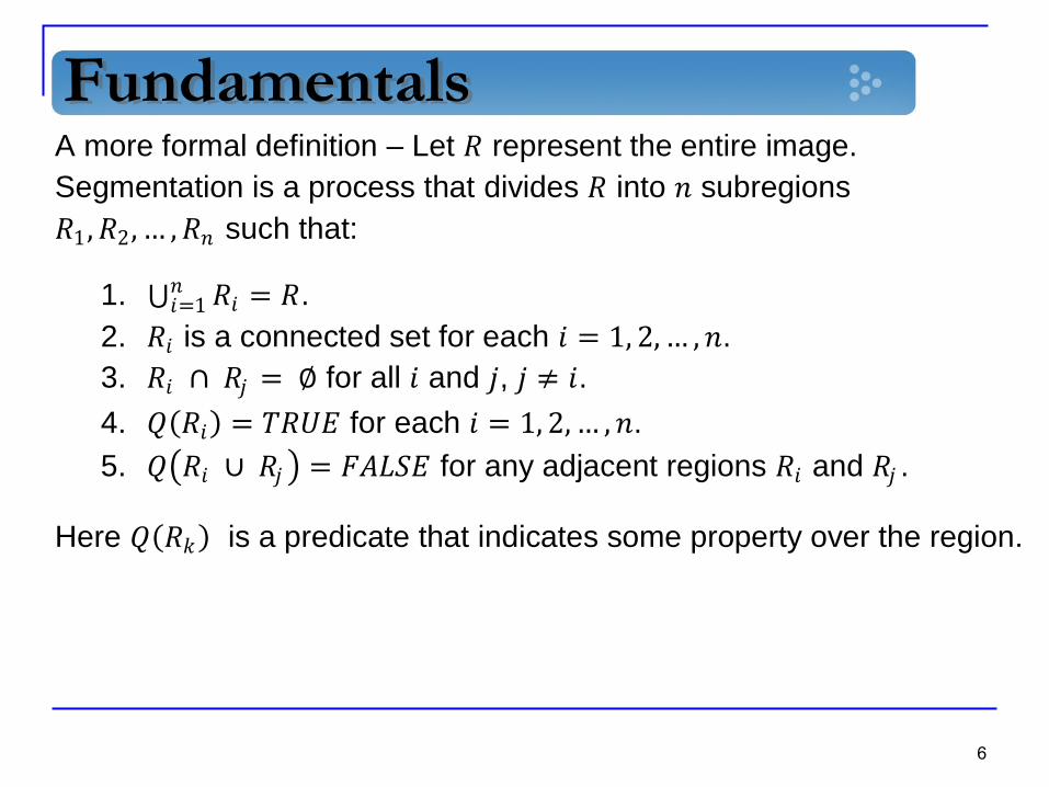
FundamentalsA more formal definition – Let 𝑅 represent the entire image.
Segmentation is a process that divides 𝑅 into 𝑛 subregions
𝑅1, 𝑅2, … , 𝑅𝑛 such that:
1. 𝑅𝑖𝑛𝑖=1 = 𝑅.
2. 𝑅𝑖 is a connected set for each 𝑖 = 1, 2, … , 𝑛.
3. 𝑅𝑖 ∩ 𝑅𝑗 = ∅ for all 𝑖 and 𝑗, 𝑗 ≠ 𝑖.
4. 𝑄 𝑅𝑖 = 𝑇𝑅𝑈𝐸 for each 𝑖 = 1, 2, … , 𝑛.
5. 𝑄 𝑅𝑖 ∪ 𝑅𝑗 = 𝐹𝐴𝐿𝑆𝐸 for any adjacent regions 𝑅𝑖 and 𝑅𝑗 .
Here 𝑄 𝑅𝑘 is a predicate that indicates some property over the region.
7
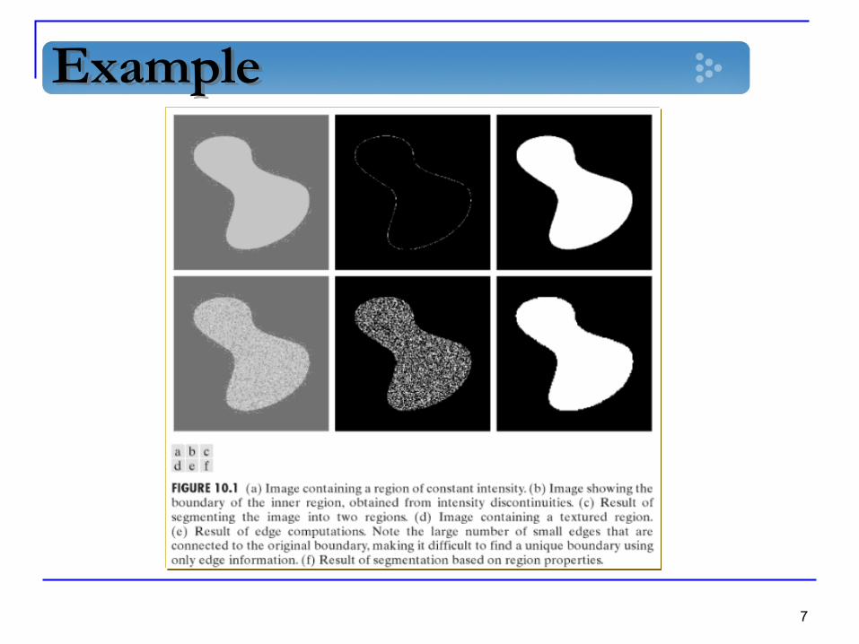
Example
8
Introduction
Mathematical background
Detection of isolated point
Line detection
Edge Models
Basic edge detection
Advanced edge detection
Edge linking and Boundary detection
Outline
9
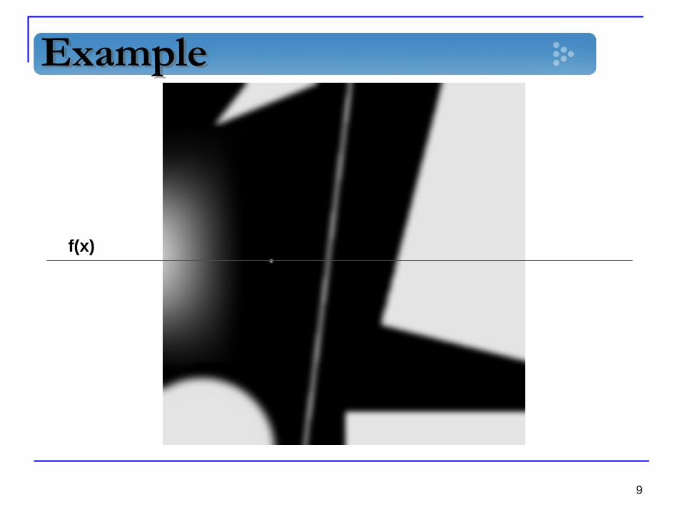
Example
f(x)
10
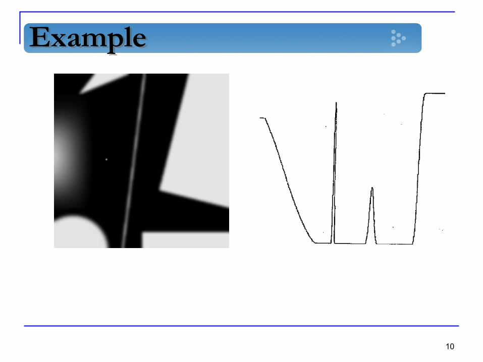
Example

11
We will use derivatives (first and second) in
order to discover discontinuities.
If we observe a line within an image we can
consider it as a one-dimensional function f(x).
We will now define the first derivative simply as
the difference between two adjacent pixels.
𝜕𝑓
𝜕𝑥= 𝑓 ′ 𝑥 = 𝑓 𝑥 + 1 − 𝑓 𝑥
𝜕2𝑓
𝜕𝑥2= 𝑓 ′′ 𝑥 = 𝑓 𝑥 + 1 − 2𝑓 𝑥 + 𝑓(𝑥 − 1)
Derivatives
12
First derivative generally produce thicker edges
in an image
Second derivative has a very strong response to
fine details and noise
Second derivative sign can be used to
determine transition direction.
Derivatives Properties
13
Derivatives - Computation
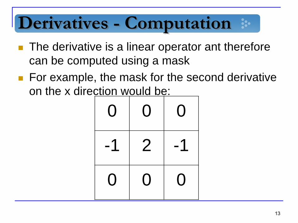
The derivative is a linear operator ant therefore
can be computed using a mask
For example, the mask for the second derivative
on the x direction would be:
0 0 0
-1 2 -1
0 0 0

14
Introduction
Mathematical background
Detection of isolated point
Line detection
Edge Models
Basic edge detection
Advanced edge detection
Edge linking and Boundary detection
Outline
15
Detection of isolated point
Based on the fact that a second order derivative
is very sensitive to sudden changes we will use
it to detect an isolated point.
We will use a Laplacian which is the second
order derivative over a two dimensional function.
16
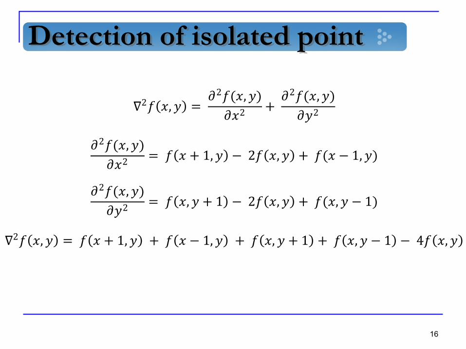
Detection of isolated point
∇2𝑓 𝑥, 𝑦 = 𝜕2𝑓(𝑥, 𝑦)
𝜕𝑥2+
𝜕2𝑓(𝑥, 𝑦)
𝜕𝑦2
𝜕2𝑓(𝑥, 𝑦)
𝜕𝑥2= 𝑓 𝑥 + 1, 𝑦 − 2𝑓 𝑥, 𝑦 + 𝑓(𝑥 − 1, 𝑦)
𝜕2𝑓(𝑥, 𝑦)
𝜕𝑦2= 𝑓 𝑥, 𝑦 + 1 − 2𝑓 𝑥, 𝑦 + 𝑓(𝑥, 𝑦 − 1)
∇2𝑓 𝑥, 𝑦 = 𝑓 𝑥 + 1, 𝑦 + 𝑓 𝑥 − 1, 𝑦 + 𝑓 𝑥, 𝑦 + 1 + 𝑓 𝑥, 𝑦 − 1 − 4𝑓 𝑥, 𝑦
17
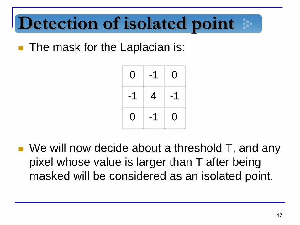
Detection of isolated point
The mask for the Laplacian is:
We will now decide about a threshold T, and any
pixel whose value is larger than T after being
masked will be considered as an isolated point.
0 -1 0
-1 4 -1
0 -1 0

18
Example
19
Introduction
Mathematical background
Detection of isolated point
Line detection
Edge Models
Basic edge detection
Advanced edge detection
Edge linking and Boundary detection
Outline

20
Line Detection
We can use the Laplacian also for detection of
line, since it is sensitive to sudden changes and
thin lines.
We must note that since the second derivative
changes its sign on a line it creates a “double
line effect” and it must be handled.
Second derivative can have negative results and
we need to scale the results

21
Double Edge Effect - Example
22
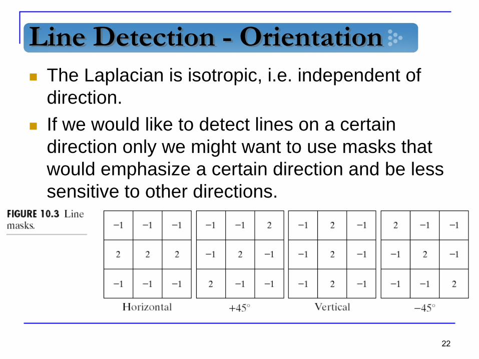
Line Detection - Orientation
The Laplacian is isotropic, i.e. independent of
direction.
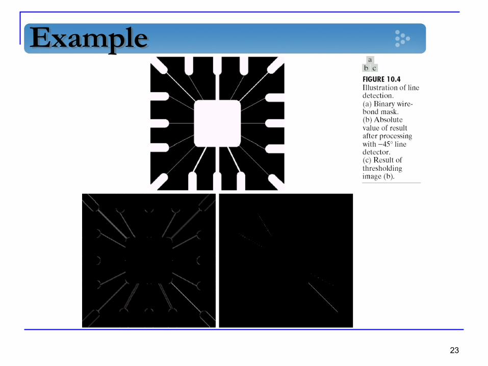
If we would like to detect lines on a certain
direction only we might want to use masks that
would emphasize a certain direction and be less
sensitive to other directions.
23
Example

24
Introduction
Mathematical background
Detection of isolated point
Line detection
Edge Models
Basic edge detection
Advanced edge detection
Edge linking and Boundary detection
Outline
25
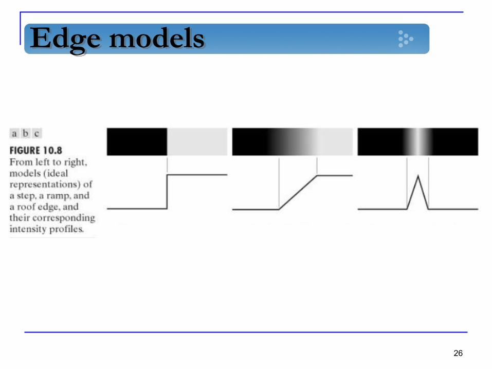
Edge models
3 differentt edge types are observed:
Step edge – Transition of intensity level over
1 pixel only in ideal, or few pixels on a more
practical use
Ramp edge – A slow and graduate transition
Roof edge – A transition to a different
intensity and back. Some kind of spread line.
26
Edge models
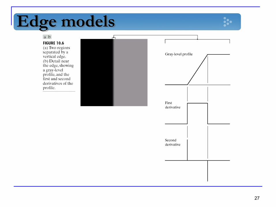
27
Edge models
28
Edge models - Derivatives
Magnitude of the first derivative can be used to
detect an edge
The sign of the second derivative indicates its
direction (black to white or white to black)
29
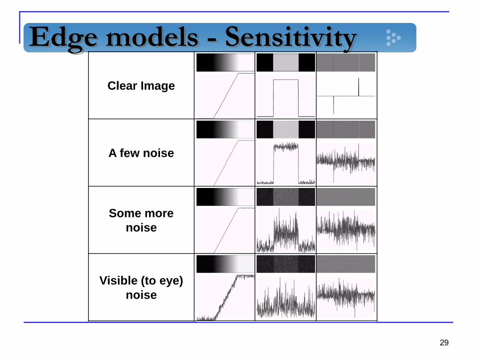
Edge models - Sensitivity
Clear Image
A few noise
Some more
noise
Visible (to eye)
noise
30
Edge models – General algorithm
It is a good practice to smooth the image before
edge detection to reduce noise.
Detect edge point – detect the points that may
be part of an edge
Select the true edge members and compose
them to an edge

31
Introduction
Mathematical background
Detection of isolated point
Line detection
Edge Models
Basic edge detection
Advanced edge detection
Edge linking and Boundary detection
Outline
32
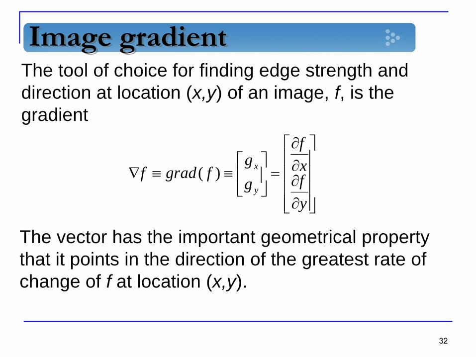
Image gradientThe tool of choice for finding edge strength and
direction at location (x,y) of an image, f, is the
gradient
The vector has the important geometrical property
that it points in the direction of the greatest rate of
change of f at location (x,y).
y
fx
f
g
gfgradf
y
x)(
Gradient Properties
33
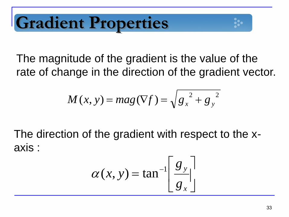
The magnitude of the gradient is the value of the
rate of change in the direction of the gradient vector.
The direction of the gradient with respect to the x-
axis :
22)(),( yx ggfmagyxM
x
y
g
gyx 1tan),(
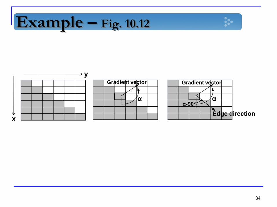
Example – Fig. 10.12
34
x
y
α α
Edge direction
α-90º
Gradient vector Gradient vector
Gradient operators
35
Instead of computing the partial derivatives at
every pixel location in the image, we will use
approximation.
Using 3x3 neighborhood centered about a point.
For gy : Subtract the pixel in the left column
from the pixel in the right column.
For gx : Subtract the pixel in the top row from
the pixel in the bottom row.
Two dimensional mask
36
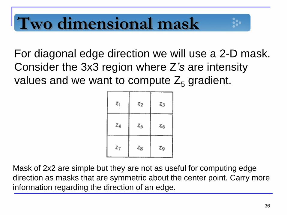
For diagonal edge direction we will use a 2-D mask.
Consider the 3x3 region where Z’s are intensity
values and we want to compute Z5 gradient.
Mask of 2x2 are simple but they are not as useful for computing edge
direction as masks that are symmetric about the center point. Carry more
information regarding the direction of an edge.
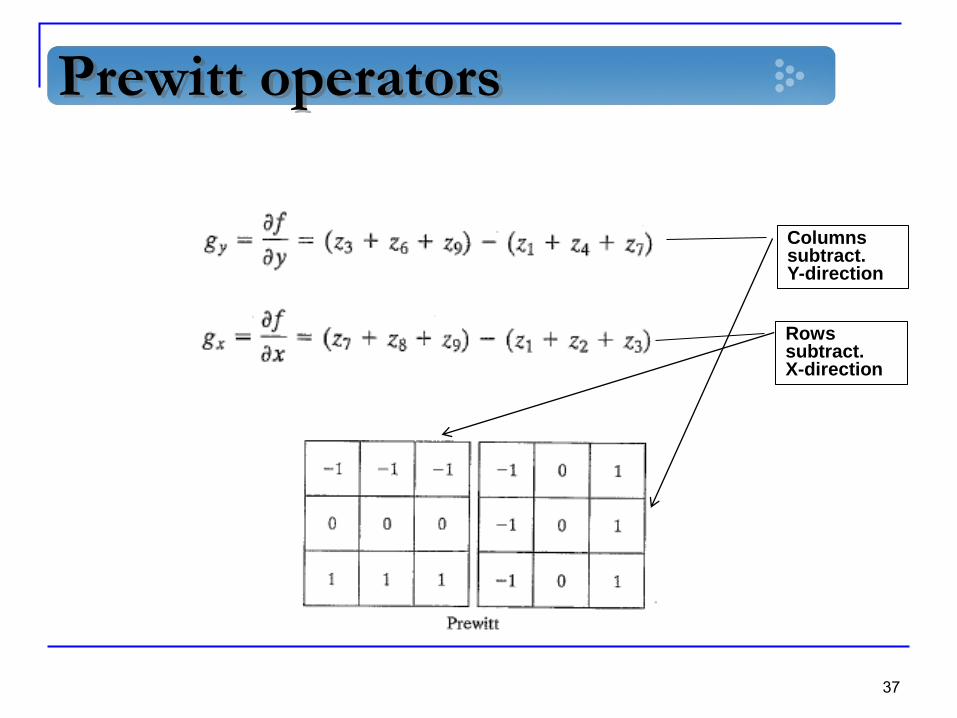
Prewitt operators
37
Rows subtract. X-direction
Columns subtract. Y-direction
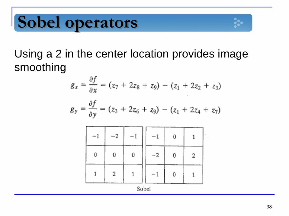
Sobel operators
38
Using a 2 in the center location provides image
smoothing
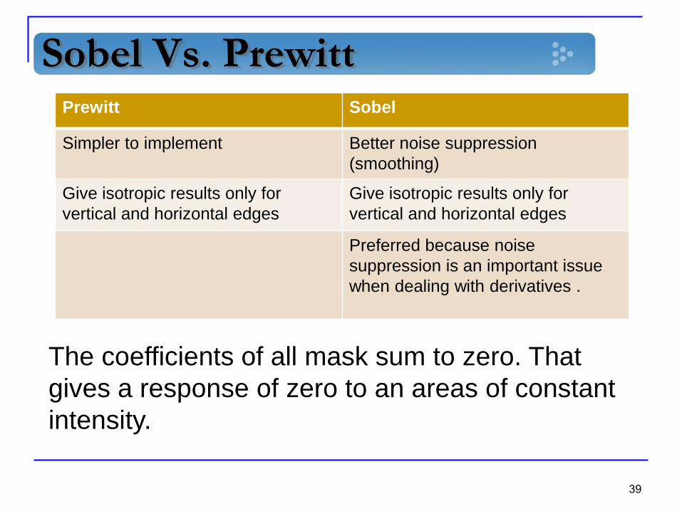
Sobel Vs. Prewitt
39
Prewitt Sobel
Simpler to implement Better noise suppression
(smoothing)
Give isotropic results only for
vertical and horizontal edges
Give isotropic results only for
vertical and horizontal edges
Preferred because noise
suppression is an important issue
when dealing with derivatives .
The coefficients of all mask sum to zero. That
gives a response of zero to an areas of constant
intensity.
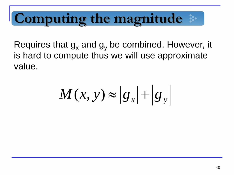
Computing the magnitude
40
Requires that gx and gy be combined. However, it
is hard to compute thus we will use approximate
value.
yx ggyxM ),(

2-D Gradient Magnitude and Angle
41
Gradient with threshold
42
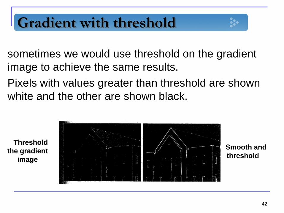
sometimes we would use threshold on the gradient
image to achieve the same results.
Pixels with values greater than threshold are shown
white and the other are shown black.
Threshold
the gradient
image
Smooth and
threshold
43
Introduction
Mathematical background
Detection of isolated point
Line detection
Edge Models
Basic edge detection
Advanced edge detection
Edge linking and Boundary detection
Outline
44
Advanced Edge detection
The basic edge detection method is based on
simple filtering without taking note of image
characteristics and other information.
More advanced techniques make attempt to
improve the simple detection by taking into
account factors such as noise, scaling etc.
We introduce 2 techniques:
Marr-Hildreth [1980]
Canny [1986]

45
Marr-Hildreth edge detector [1980]
Marr and Hildreth argued that:
Intensity of changes is not independent of
image scale
Sudden intensity change will cause a zero-
crossing of the second derivative
Therefore, an edge detection operator should:
Be capable of being tuned to any scale
Be capable of computing the first and second
derivatives

46
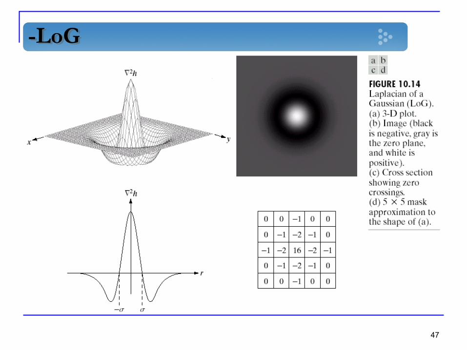
Marr-Hildreth edge detector [1980]
They used the operator ∇2𝐺 where ∇2 is the Laplacian and 𝐺 is the
2-D Gaussian function 𝐺 𝑥, 𝑦 = 𝑒−
𝑥2+𝑦2
2𝜎2 with standard deviation 𝜎.
And we get ∇2𝐺(𝑥, 𝑦) = 𝑥2+𝑦2−2𝜎2
𝜎4 𝑒
−𝑥2+𝑦2
2𝜎2 , also called Laplacian
of Gaussian (LoG).
47
-LoG
48
What does it do?
The Gaussian blurs the image by reducing the
intensity of structures (such as noise) at scales
much lower than σ.
The Laplacian part is responsible for detecting
the edges due to the sensitivity of second
derivative.
Since filter is linear action these two filters can
be applied separately, thus allowing us to use
different sized filters for each of the actions.
49
The algorithm
The algorithm is:
Filter image with nxn Gaussian filter
Compute the Laplacian using for example a
3x3 mask.
Find the zero crossings
To find a zero crossing it is possible to use 3x3
mask that checks sign changes around a pixel.
Sometimes it is suggested to use the algorithm
with different σ and then to combine the results.

51
Canny edge detector
Three basic objectives:
Low error rate – Edge detected must be as
close as possible to the true edge.
Single edge point response – The detector
should return only one point for each true
edge point.
52
Step 1 – Smooth image
Create a smoothed image from the original one
using Gaussian function.
𝐺 𝑥, 𝑦 = 𝑒−
𝑥2+𝑦2
2𝜎2
𝑓𝑠 𝑥, 𝑦 = 𝐺(𝑥, 𝑦)𝑓(𝑥, 𝑦)
53
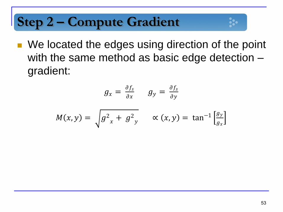
Step 2 – Compute Gradient
We located the edges using direction of the point
with the same method as basic edge detection –
gradient:
𝑔𝑥 = 𝜕𝑓𝑠
𝜕𝑥 𝑔𝑦 =
𝜕𝑓𝑠
𝜕𝑦
𝑀 𝑥, 𝑦 = 𝑔2𝑥
+ 𝑔2𝑦 ∝ 𝑥, 𝑦 = tan−1
𝑔𝑦
𝑔𝑥
54
Step 3 – Nonmaxima suppression
Edges generated using gradient typically contain
wide ridges around local maxima.
We will locate the local maxima using non-
maxima suppression method.
We will define a number of discrete orientations.
For example in a 3x3 region 4 direction can be
defined.

55
Step 3 – Nonmaxima suppression
56
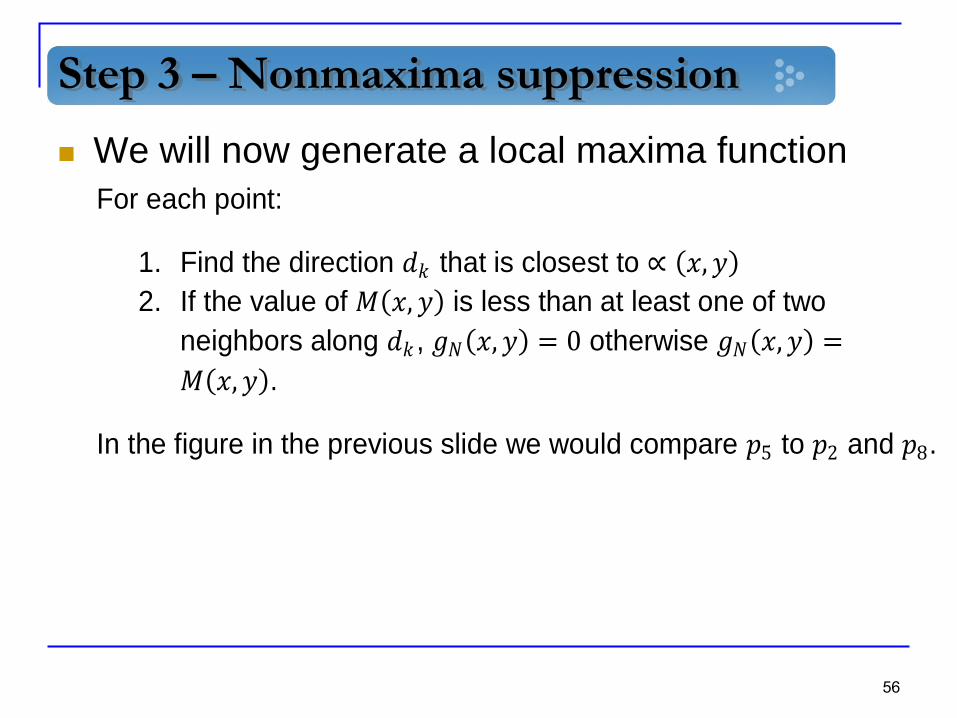
Step 3 – Nonmaxima suppression
We will now generate a local maxima function
For each point:
1. Find the direction 𝑑𝑘 that is closest to ∝ 𝑥, 𝑦
2. If the value of 𝑀 𝑥, 𝑦 is less than at least one of two
neighbors along 𝑑𝑘 , 𝑔𝑁 𝑥, 𝑦 = 0 otherwise 𝑔𝑁 𝑥, 𝑦 =
𝑀 𝑥, 𝑦 .
In the figure in the previous slide we would compare 𝑝5 to 𝑝2 and 𝑝8.
57
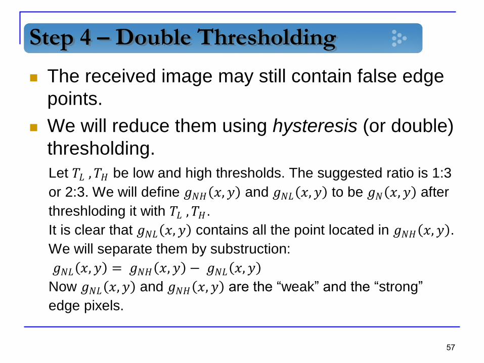
Step 4 – Double Thresholding
The received image may still contain false edge
points.
We will reduce them using hysteresis (or double)
thresholding.
Let 𝑇𝐿 , 𝑇𝐻 be low and high thresholds. The suggested ratio is 1:3
or 2:3. We will define 𝑔𝑁𝐻 𝑥, 𝑦 and 𝑔𝑁𝐿 𝑥, 𝑦 to be 𝑔𝑁 𝑥, 𝑦 after
threshloding it with 𝑇𝐿 , 𝑇𝐻.
It is clear that 𝑔𝑁𝐿 𝑥, 𝑦 contains all the point located in 𝑔𝑁𝐻 𝑥, 𝑦 .
We will separate them by substruction:
𝑔𝑁𝐿 𝑥, 𝑦 = 𝑔𝑁𝐻 𝑥, 𝑦 − 𝑔𝑁𝐿 𝑥, 𝑦
Now 𝑔𝑁𝐿 𝑥, 𝑦 and 𝑔𝑁𝐻 𝑥, 𝑦 are the “weak” and the “strong”
edge pixels.
58
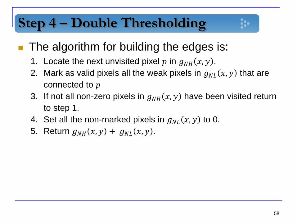
Step 4 – Double Thresholding
The algorithm for building the edges is:1. Locate the next unvisited pixel 𝑝 in 𝑔𝑁𝐻 𝑥, 𝑦 .
2. Mark as valid pixels all the weak pixels in 𝑔𝑁𝐿 𝑥, 𝑦 that are
connected to 𝑝
3. If not all non-zero pixels in 𝑔𝑁𝐻 𝑥, 𝑦 have been visited return
to step 1.
4. Set all the non-marked pixels in 𝑔𝑁𝐿 𝑥, 𝑦 to 0.
5. Return 𝑔𝑁𝐻 𝑥, 𝑦 + 𝑔𝑁𝐿 𝑥, 𝑦 .
61
Introduction
Mathematical background
Detection of isolated point
Line detection
Edge Models
Basic edge detection
Advanced edge detection
Edge linking and Boundary detection
Outline

62
Edge Linking introduction
Ideally, edge detection should yield sets of pixels
lying only on edges. In practice, these pixels seldom
characterize edges completely because of noise or
breaks in the edges.
Therefore, edge detection typically is followed by
linking algorithms designed to assemble edge pixels
into meaningful edges and/or region boundaries.
We will introduce two linking techniques.
Local processing
63
All points that are similar according to predefined
criteria are linked, forming an edge of pixels that
share common properties.
Similarity according to:
1. Strength (magnitude)
2. Direction of the gradient vector
Local processing
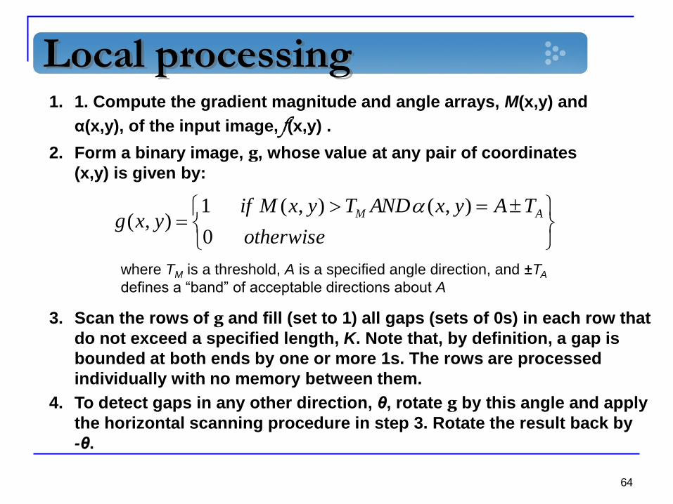
64
1. 1. Compute the gradient magnitude and angle arrays, M(x,y) and
α(x,y), of the input image, f(x,y) .
2. Form a binary image, g, whose value at any pair of coordinates
(x,y) is given by:
otherwise
TAyxANDTyxMifyxg
AM
0
),(),(1),(
where TM is a threshold, A is a specified angle direction, and ±TA
defines a “band” of acceptable directions about A
3. Scan the rows of g and fill (set to 1) all gaps (sets of 0s) in each row that
do not exceed a specified length, K. Note that, by definition, a gap is
bounded at both ends by one or more 1s. The rows are processed
individually with no memory between them.
4. To detect gaps in any other direction, θ, rotate g by this angle and apply
the horizontal scanning procedure in step 3. Rotate the result back by
-θ.
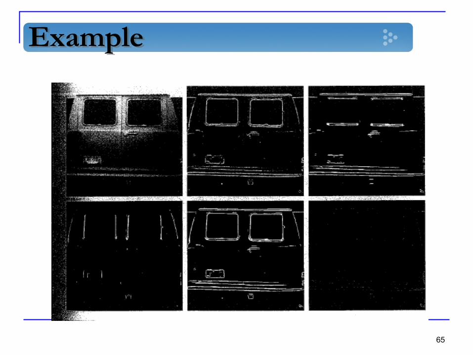
Example
65

Global processing
Good for unstructured environments.
All pixels are candidate for linking.
Need for predefined global properties.
What we are looking for?
Decide whether sets of pixels lie on curves of
a specified shape.
66
Trivial application
Given n points.
We want to find subset of n that lie on straight
lines:
Find all lines determined by every pair of points
Find all subset of points that are close to particular
lines.
n*(n-1)/2 + n*(n*(n-1))/2 ~ n^2+ n^3.
Too hard to compute.
67
Hough transform
The xy-plane:
Consider a point (xi,yi). The general equation
of a straight line : yi = axi +b.
Many lines pass through (xi,yi). They all
satisfy : yi = axi +b for varying values of a and
b.
68
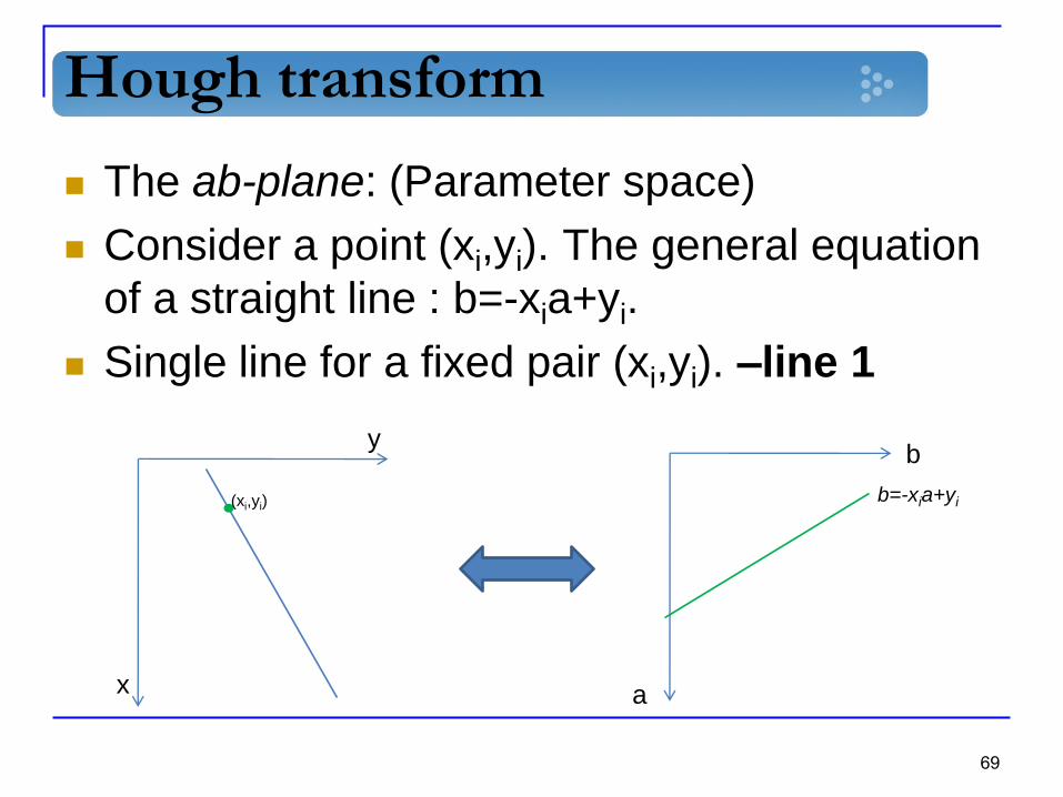
Hough transform
The ab-plane: (Parameter space)
Consider a point (xi,yi). The general equation
of a straight line : b=-xia+yi.
Single line for a fixed pair (xi,yi). –line 1
69
b=-xia+yi
y
x
(xi,yi)
b
a
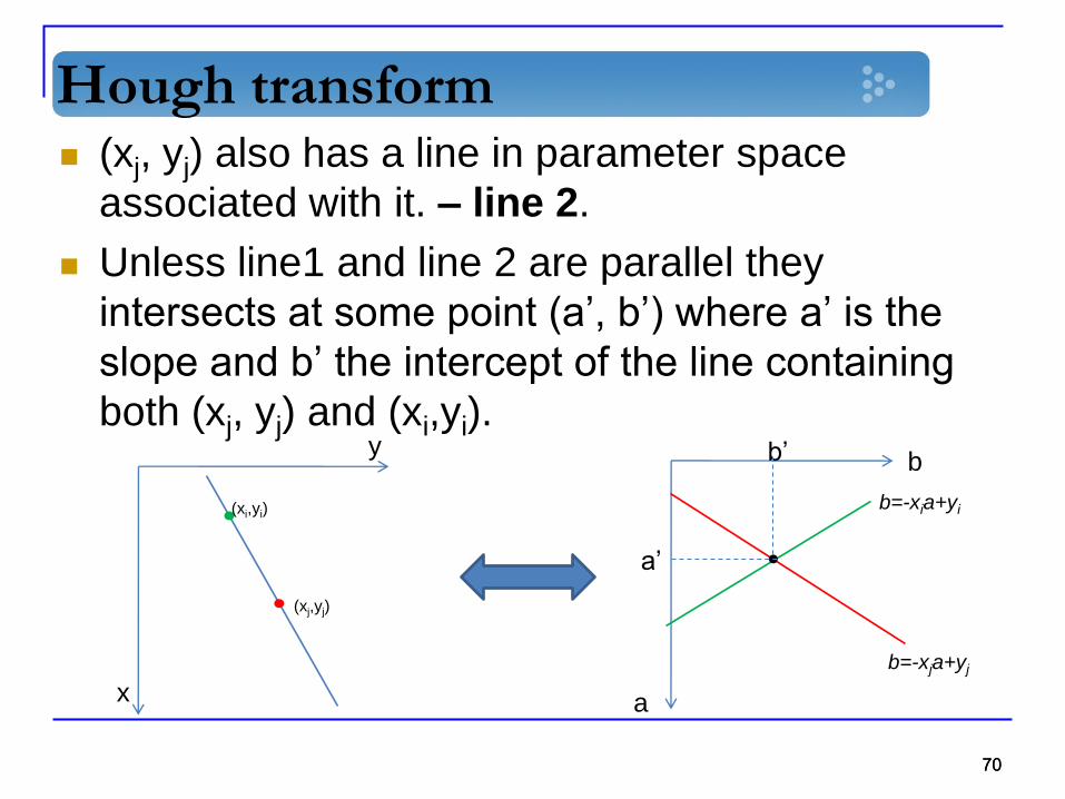
Hough transform (xj, yj) also has a line in parameter space
associated with it. – line 2.
Unless line1 and line 2 are parallel they
intersects at some point (a’, b’) where a’ is the
slope and b’ the intercept of the line containing
both (xj, yj) and (xi,yi).
7070
b=-xia+yi
y
x
(xi,yi)
b
a
(xj,yj)
b’
a’
b=-xja+yj

Hough transform
Parameter – space lines corresponding to all
points (xk,yk) in the xy-plane could be plotted
and the principal lines in that plane could be
found by identifying points in parameter
space where large numbers of lines intersect.
71

Hough transform
Using yi=axi+b approaches infinity when lines
approach the vertical direction.
72
ysincosx Normal representation of a line.
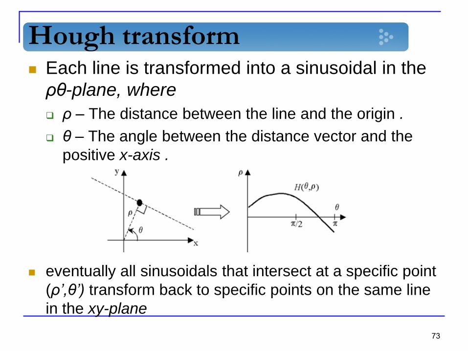
Hough transform Each line is transformed into a sinusoidal in the
ρθ-plane, where
ρ – The distance between the line and the origin .
θ – The angle between the distance vector and the
positive x-axis .
eventually all sinusoidals that intersect at a specific point
(ρ’,θ’) transform back to specific points on the same line
in the xy-plane
73
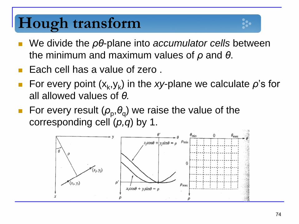
Hough transform We divide the ρθ-plane into accumulator cells between
the minimum and maximum values of ρ and θ.
Each cell has a value of zero .
For every point (xk,yk) in the xy-plane we calculate ρ’s for
all allowed values of θ.
For every result (ρp,θq) we raise the value of the
corresponding cell (p,q) by 1.
74
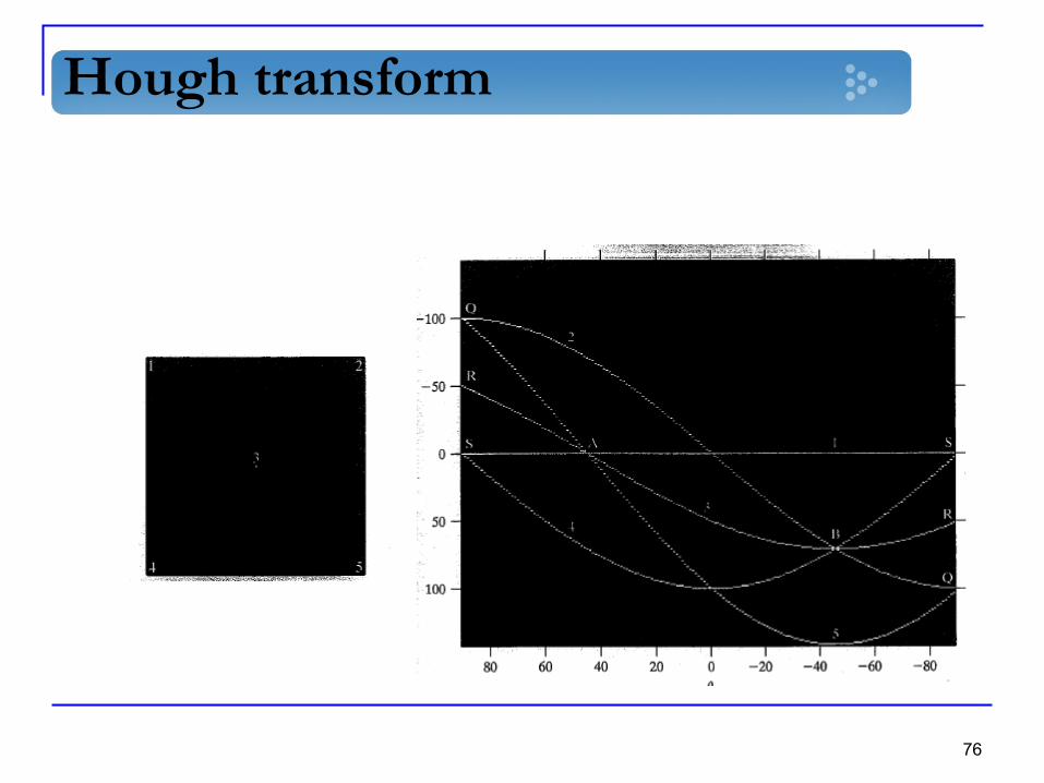
Hough transform
At the end of the process, the value P of the
cell A(i,j) represents a number of P points in
the xy-plane that lie on the
line.
The number of sub-divisions determines the
accuracy of the co-linearity of the points.
75
ijyjx sincos
Hough transform
76

Hough transform
77
45deg
0
-45deg
71

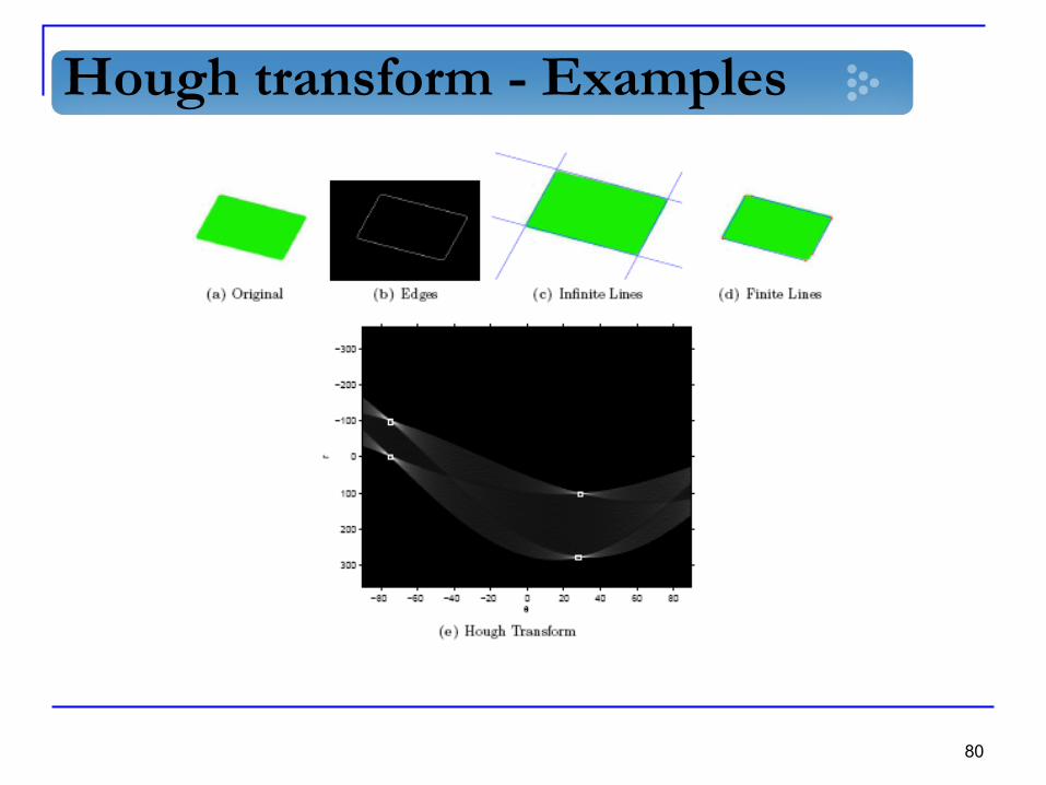
Hough transform – Edge linking
Algorithm :
1. Obtain a binary edge image using any of the
techniques discussed earlier in this section
2. Specify subdivisions in the ρθ –plane.
3. Examine the counts of the accumulator cells for
high pixel concentrations .
4. Examine the relationships (principally for
continuity) between pixels in a chosen cell .
78

Hough transform - Examples
79
Hough transform - Examples
80

81
Questions?

82
Thank You!