Embed Size (px)
Citation preview
2011-04-06
DDigital Image Processing
Achim J. Lilienthal
AASS Learning Systems Lab, Dep. Teknik
Room T1209 (Fr, 11-12 o'clock)
Course Book Chapter 3
Part 2: Image Enhancement
in the Spatial Domain

Achim J. Lilienthal
1. Image Enhancement in the Spatial Domain
2. Grey Level Transformations
3. Histogram Processing
4. Operations Involving Multiple Images
5. Spatial Filtering
Contents��1. Image Enhancement in the Spatial Domain
2. Grey Level Transformations
3. Histogram Processing
4. Operations Involving Multiple Images
5. Spatial Filtering

Achim J. Lilienthal
Image Enhancement in the Spatial Domain
� Contents� Contents
Achim J. Lilienthal
Image Enhancement in the Spatial Domain1
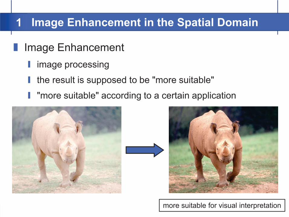
� Image Enhancement� image processing
� the result is supposed to be "more suitable"
� "more suitable" according to a certain application
more suitable for visual interpretation
Achim J. Lilienthal
Image Enhancement in the Spatial Domain1
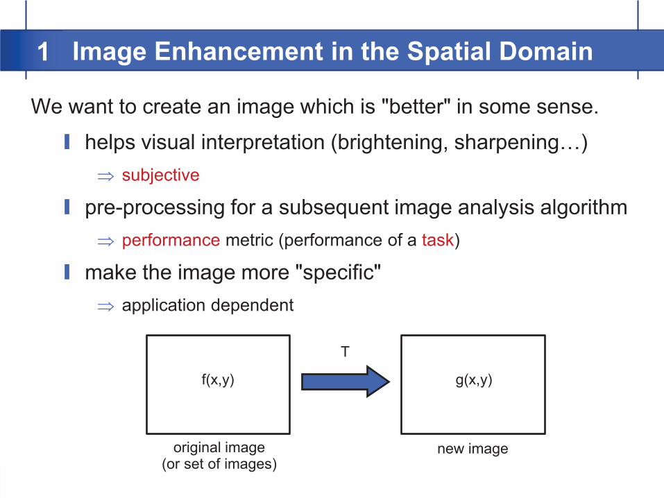
We want to create an image which is "better" in some sense.
� helps visual interpretation (brightening, sharpening…)� subjective
� pre-processing for a subsequent image analysis algorithm� performance metric (performance of a task)
� make the image more "specific" � application dependent
f(x,y) g(x,y)
original image(or set of images)
new image
T
Achim J. Lilienthal
Image Enhancement in the Spatial Domain1
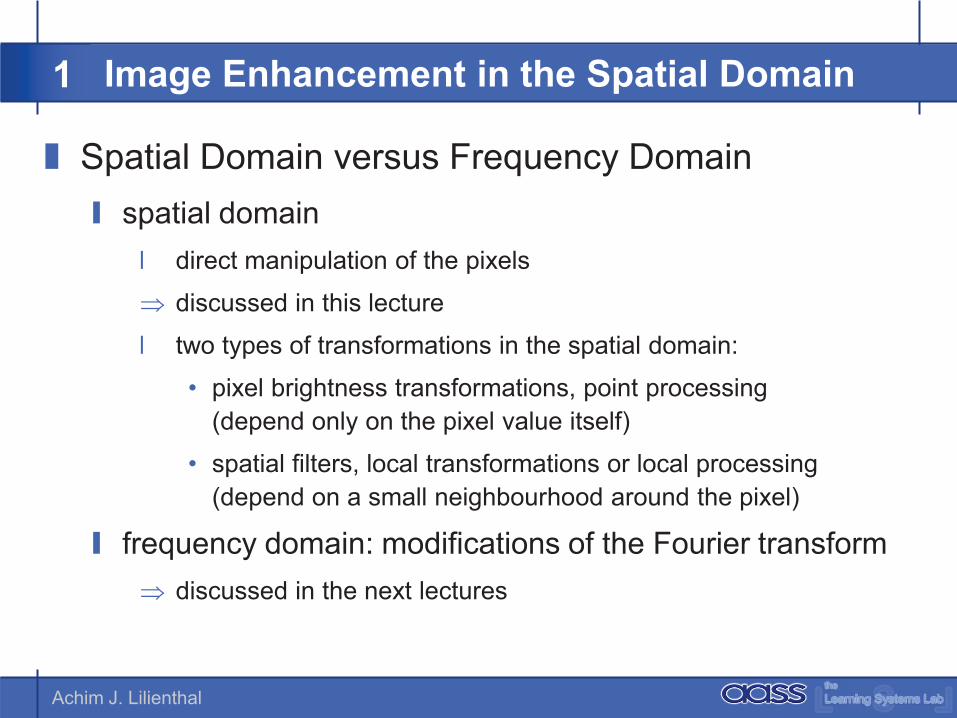
� Spatial Domain versus Frequency Domain� spatial domain
� direct manipulation of the pixels
� discussed in this lecture
� two types of transformations in the spatial domain:
� pixel brightness transformations, point processing(depend only on the pixel value itself)
� spatial filters, local transformations or local processing(depend on a small neighbourhood around the pixel)
� frequency domain: modifications of the Fourier transform� discussed in the next lectures
Achim J. Lilienthal
Image Enhancement in the Spatial Domain1
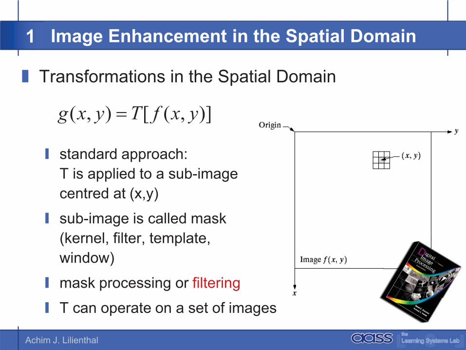
� Transformations in the Spatial Domain
� standard approach:T is applied to a sub-image centred at (x,y)
� sub-image is called mask(kernel, filter, template, window)
� mask processing or filtering
� T can operate on a set of images
)],([),( yxfTyxg �
Achim J. Lilienthal
Image Enhancement in the Spatial Domain1
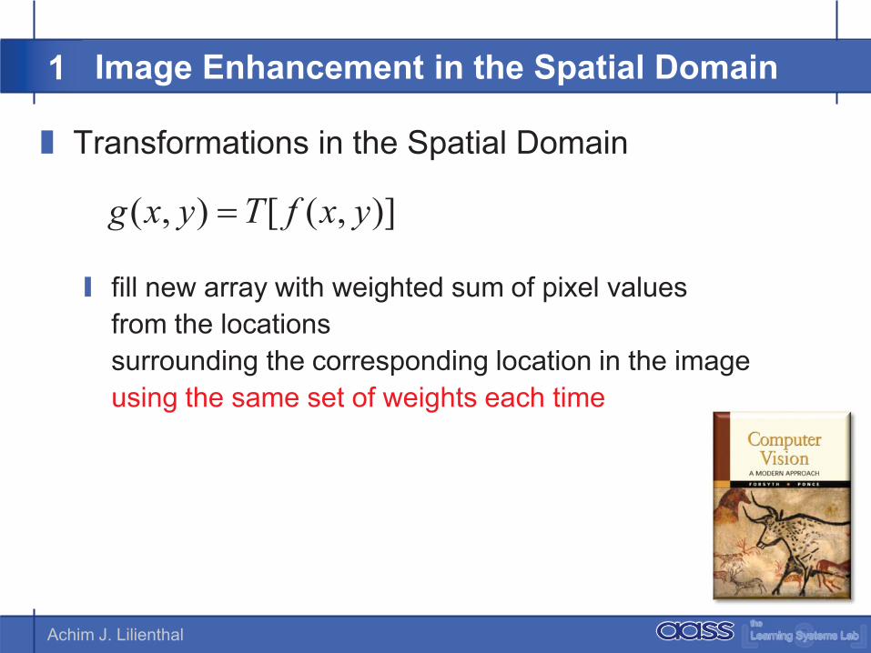
� Transformations in the Spatial Domain
� fill new array with weighted sum of pixel values from the locations surrounding the corresponding location in the image using the same set of weights each time
)],([),( yxfTyxg �

Achim J. Lilienthal
Gray Level Transformations
� Contents� Contents
Achim J. Lilienthal
Grey Level Transformations2
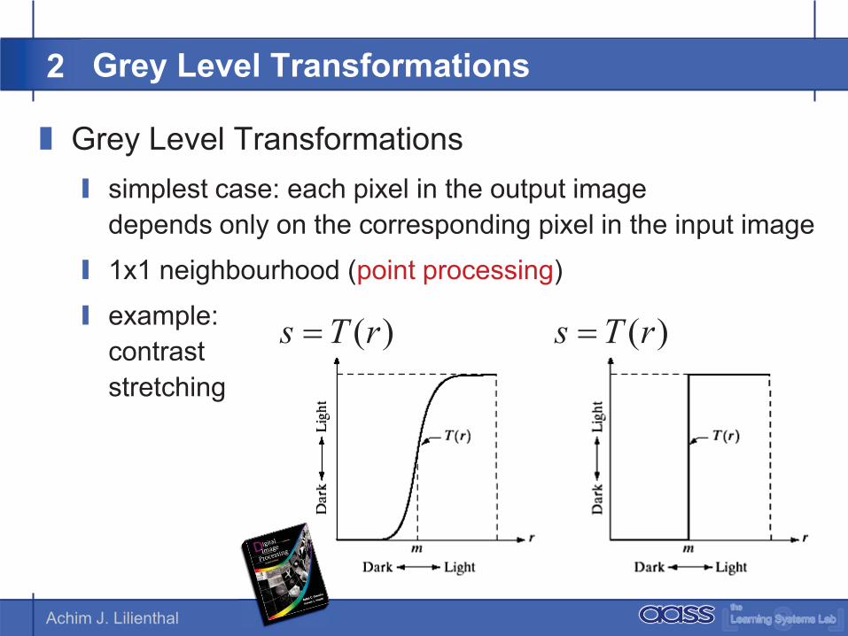
� Grey Level Transformations� simplest case: each pixel in the output image
depends only on the corresponding pixel in the input image
� 1x1 neighbourhood (point processing)
� example:contraststretching
)(rTs �)(rTs �
Achim J. Lilienthal
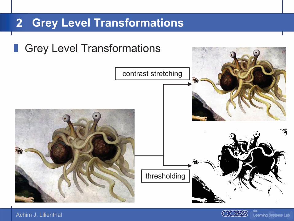
� Grey Level Transformations
contrast stretching
thresholding
Grey Level Transformations2

Achim J. Lilienthal
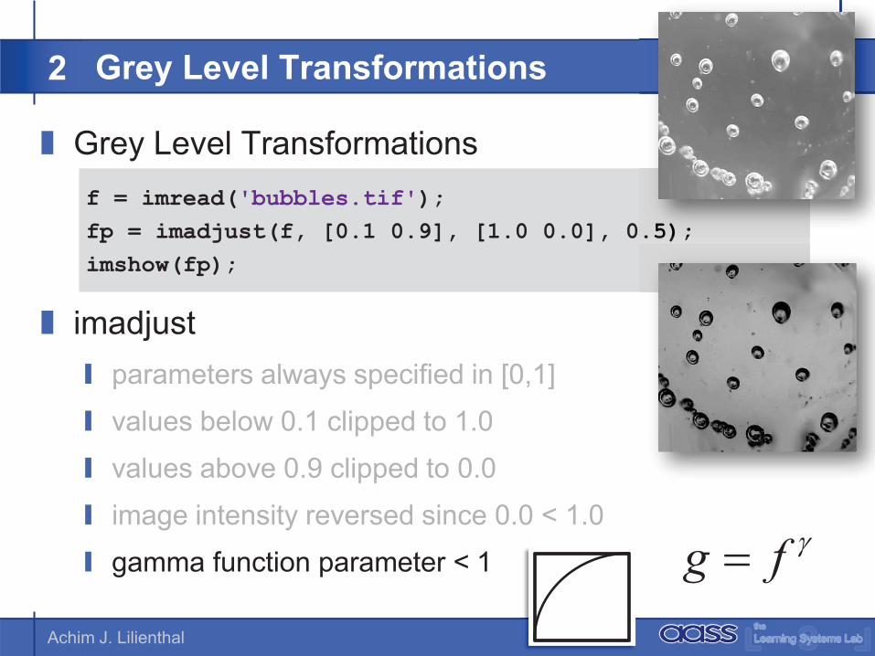
� Grey Level Transformations
� imadjust� parameters always specified in [0,1]
� values below 0.1 clipped to 1.0
� values above 0.9 clipped to 0.0
� image intensity reversed since 0.0 < 1.0
Grey Level Transformations2
f = imread('bubbles.tif');fp = imadjust(f, [0.1 0.9], [1.0 0.0], 0.5);imshow(fp);
.5);
Achim J. Lilienthal
� Grey Level Transformations
� imadjust� parameters always specified in [0,1]
� values below 0.1 clipped to 1.0
� values above 0.9 clipped to 0.0
� image intensity reversed since 0.0 < 1.0
� gamma function parameter < 1
Grey Level Transformations2
f = imread('bubbles.tif');fp = imadjust(f, [0.1 0.9], [1.0 0.0], 0.5);imshow(fp);
.5);
g f ��

Achim J. Lilienthal
� Grey Level Transformations
Grey Level Transformations2
f = imread('bubbles.tif');fp = imadjust(f, [0.1 0.9], [1.0 0.0], 0.5);imshow(fp);
.5);
fp = imadjust(f, [0.55 0.9], [1.0 0.0], 3);3);
Achim J. Lilienthal
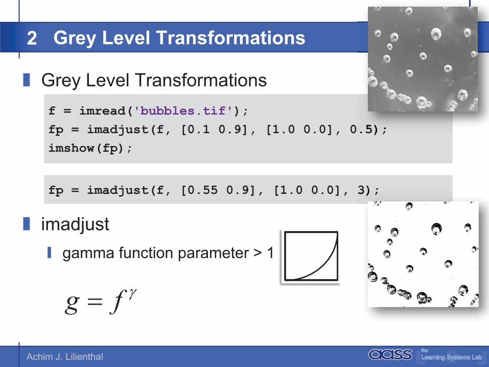
� Grey Level Transformations
� imadjust� gamma function parameter > 1
Grey Level Transformations2
f = imread('bubbles.tif');fp = imadjust(f, [0.1 0.9], [1.0 0.0], 0.5);imshow(fp);
.5);
fp = imadjust(f, [0.55 0.9], [1.0 0.0], 3);
g f ��
3);
Achim J. Lilienthal
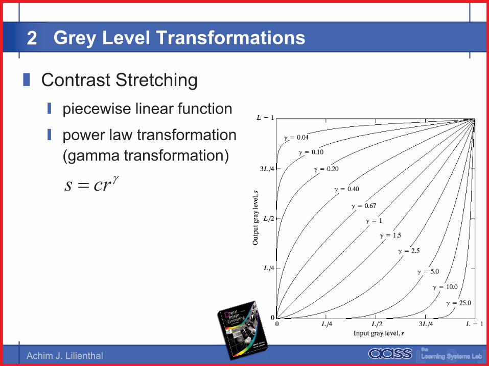
� Contrast Stretching� piecewise linear function
� power law transformation(gamma transformation)
�crs �
Grey Level Transformations2
Achim J. Lilienthal
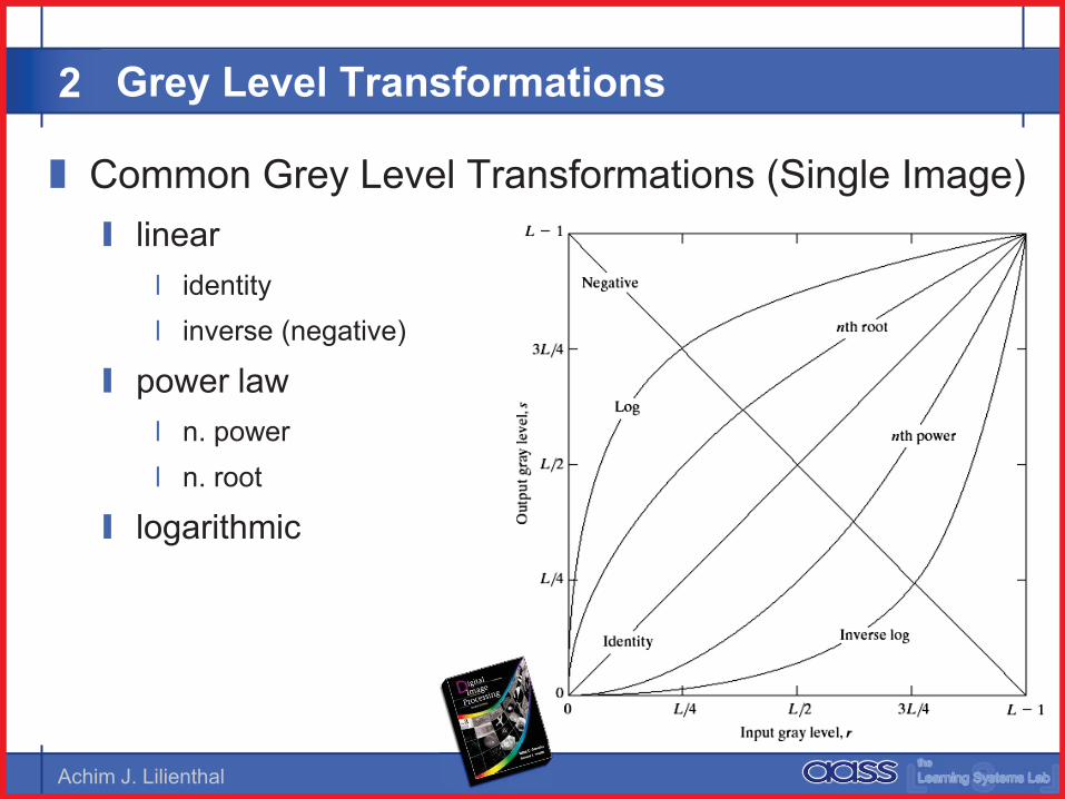
� Common Grey Level Transformations (Single Image)� linear
� identity� inverse (negative)
� power law� n. power� n. root
� logarithmic
Grey Level Transformations2
Achim J. Lilienthal
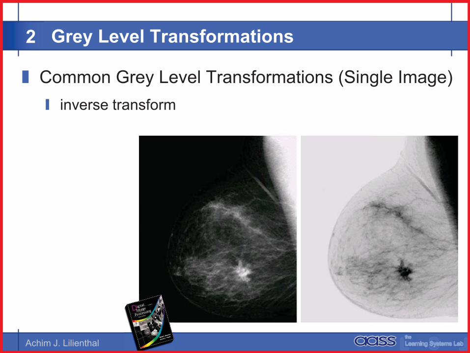
� Common Grey Level Transformations (Single Image)� inverse transform
Grey Level Transformations2

Achim J. Lilienthal
� Contrast Stretching� piecewise linear function
Grey Level Transformations2
Achim J. Lilienthal
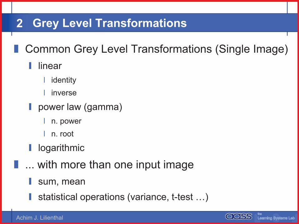
� Common Grey Level Transformations (Single Image)� linear
� identity� inverse
� power law (gamma)� n. power� n. root
� logarithmic
� ... with more than one input image� sum, mean� statistical operations (variance, t-test …)
Grey Level Transformations2
Achim J. Lilienthal
Histogram Processing
� Contents� Contents

Achim J. Lilienthal
Histogram Processing3
� Grey Scale Histogram� shows the number of pixels per grey level
f = imread('bubbles.tif');imhist(f); % displays the histogram
% histogram display default splay default
Achim J. Lilienthal
Histogram Processing3
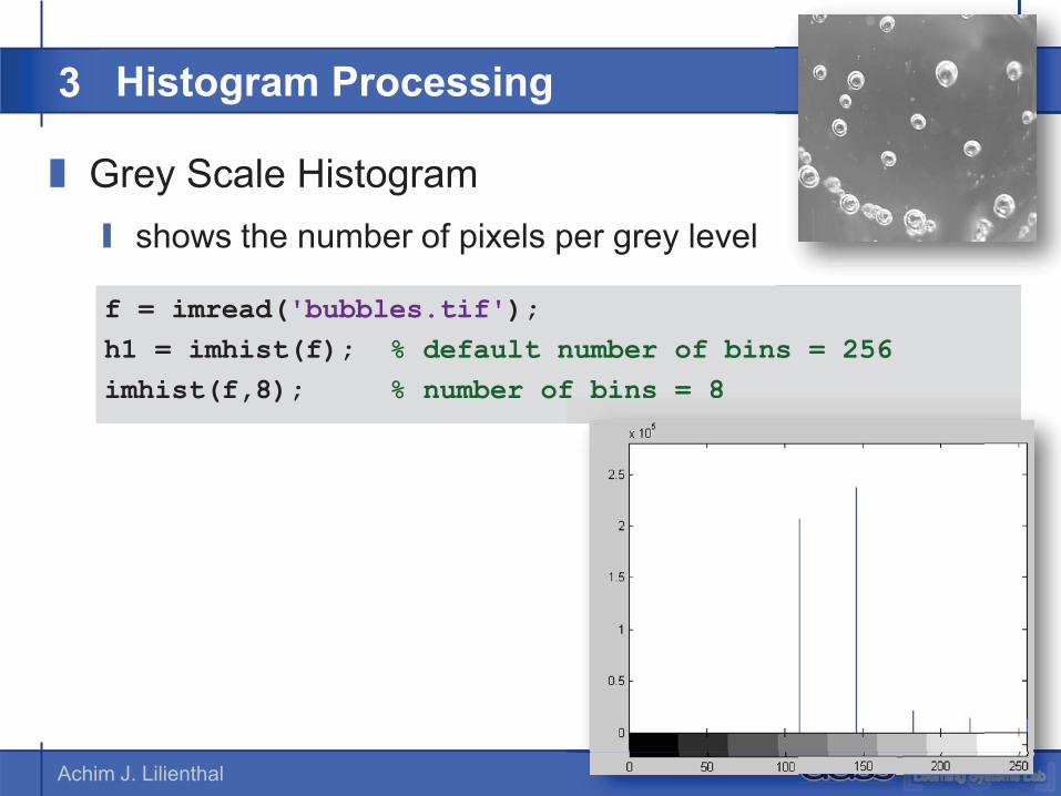
� Grey Scale Histogram� shows the number of pixels per grey level
f = imread('bubbles.tif');h1 = imhist(f); % default number of bins = 256imhist(f,8); % number of bins = 8f bins 8
Achim J. Lilienthal
Histogram Processing3
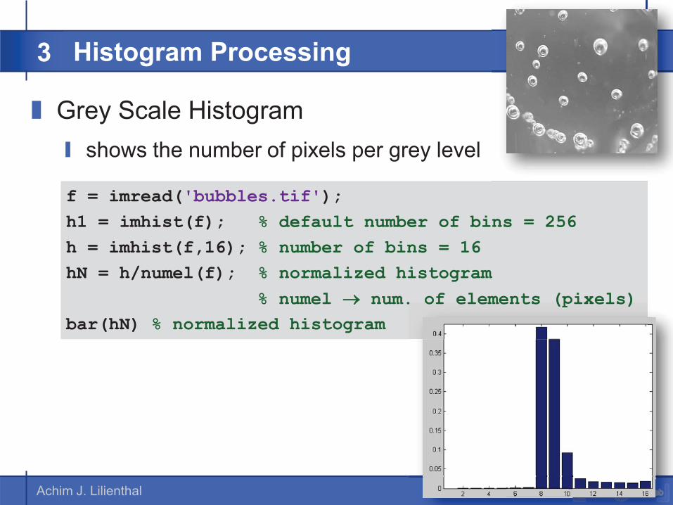
� Grey Scale Histogram� shows the number of pixels per grey level
f = imread('bubbles.tif');h1 = imhist(f); % default number of bins = 256h = imhist(f,16); % number of bins = 16hN = h/numel(f); % normalized histogram
% numel �� num. of elements (pixels)bar(hN) % normalized histogram
. of elements (pixels)
Achim J. Lilienthal
Histogram Processing3
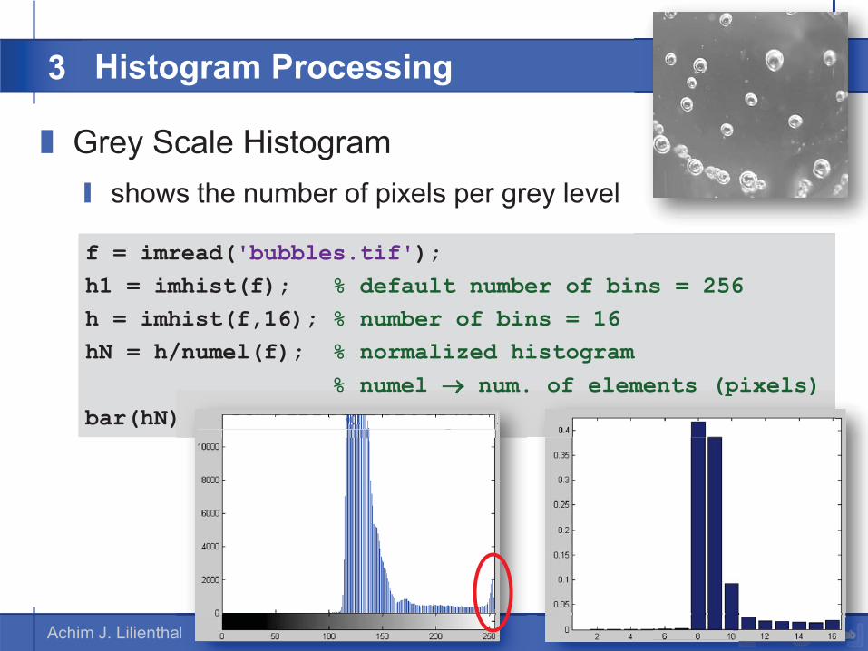
� Grey Scale Histogram� shows the number of pixels per grey level
f = imread('bubbles.tif');h1 = imhist(f); % default number of bins = 256h = imhist(f,16); % number of bins = 16hN = h/numel(f); % normalized histogram
% numel � num. of elements (pixels)bar(hN) % normalized histogram
of elements (pixels)
al
% numel � num.
. % nnnnnooooorrrrrmmmmmmaaaaallllliiiiizzzzeeeeeddddddddd hhhhhhiiiiissssstttttooooogggggrrrrraaaaammmmmmm
Achim J. Lilienthal
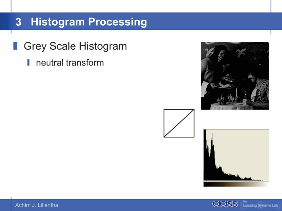
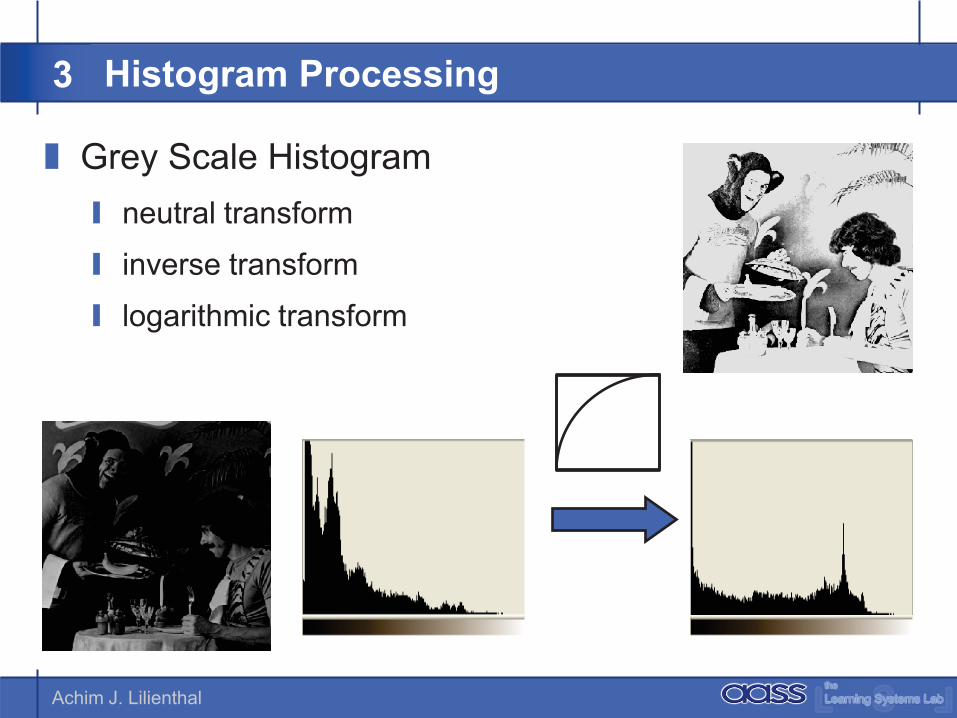
� Grey Scale Histogram� neutral transform
Histogram Processing3
Achim J. Lilienthal
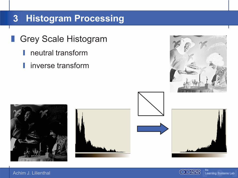
� Grey Scale Histogram� neutral transform
� inverse transform
Histogram Processing3
Achim J. Lilienthal
� Grey Scale Histogram� neutral transform
� inverse transform
� logarithmic transform
Histogram Processing3
Achim J. Lilienthal
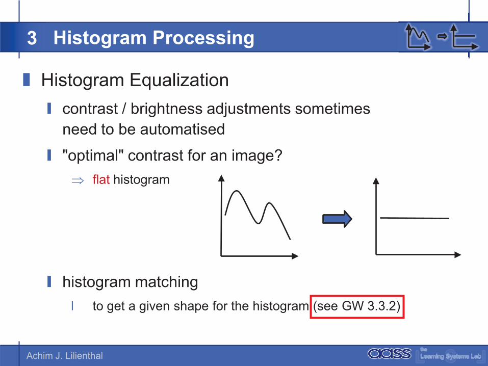
� Histogram Equalization� contrast / brightness adjustments sometimes
need to be automatised
� "optimal" contrast for an image?� flat histogram
� histogram matching� to get a given shape for the histogram (see GW 3.3.2)
Histogram Processing3

Achim J. Lilienthal
� Histogram Equalization� consider the continuous case:
� probability density functions (PDFs) of s and r are related by
� transformation function = cumulative density function (CDF)
� �
]1,0[, �rs
)(1)()()(rT
rpdsdrrpsp rrs �
��
)()()(0
rpdpdrdrT
drds
r
r
r ��
��
��� � �� 1)( �sps
Histogram Processing3
gray levels as random variables!
�� )(rTs
��r
r dprT0
)()( ��

Achim J. Lilienthal
� Histogram Equalization� discrete case
� does not generally produce a uniform PDF
� tends to spread the histogram
� enables automatic contrast stretching
nnrp k
kr �)( ����
���k
j
jk
jjrkk n
nrprTs
00)()(
Histogram Processing3
Achim J. Lilienthal
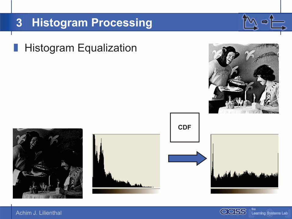
� Histogram Equalization
CDF
Histogram Processing3
Achim J. Lilienthal
� Histogram Equalization
Histogram Processing3

Achim J. Lilienthal
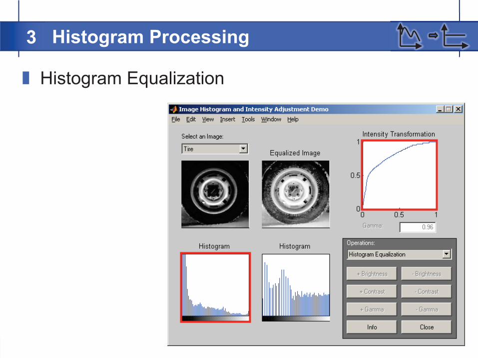
� Histogram Equalization
Histogram Processing3
f = imread('bubbles.tif');g = histeq(f, 256);imshow(g);
f = imread('bubbles.tif');g = histeq(f, 4); % 4 output levelsimshow(g);
Achim J. Lilienthal
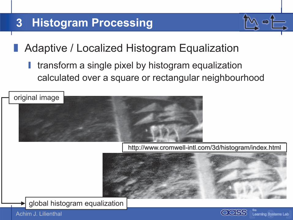
� Adaptive / Localized Histogram Equalization� transform a single pixel by histogram equalization
calculated over a square or rectangular neighbourhood
original image
global histogram equalization
Histogram Processing3
http://www.cromwell-intl.com/3d/histogram/index.html
Achim J. Lilienthal
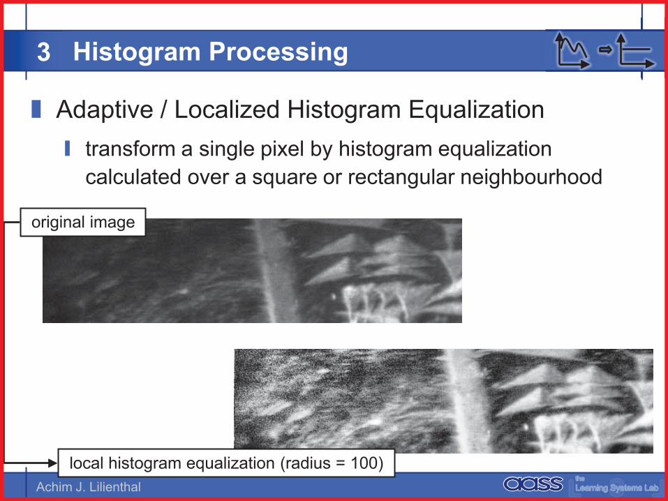
� Adaptive / Localized Histogram Equalization� transform a single pixel by histogram equalization
calculated over a square or rectangular neighbourhood
original image
local histogram equalization (radius = 100)
Histogram Processing3

Achim J. Lilienthal
� Adaptive / Localized Histogram Equalization� transform a single pixel by histogram equalization
calculated over a square or rectangular neighbourhood
original image
local histogram equalization (radius = 50)
Histogram Processing3

Achim J. Lilienthal
� Adaptive / Localized Histogram Equalization� transform a single pixel by histogram equalization
calculated over a square or rectangular neighbourhood
original image
local histogram equalization (radius = 25)
Histogram Processing3

Achim J. Lilienthal
� Adaptive / Localized Histogram Equalization� transform a single pixel by histogram equalization
calculated over a square or rectangular neighbourhood
original image
local histogram equalization (radius = 12)
Histogram Processing3

Achim J. Lilienthal
Operations Involving Multiple Images
� Contents� Contents
Achim J. Lilienthal
� Operations Between Two or More Images� image subtraction
� Arteriography
� tracking
Operations Involving Multiple Images4

Achim J. Lilienthal
� Image Subtraction� DSA (Digital Subtraction Arteriography)
Operations Involving Multiple Images4
mask image live image DSA image
Achim J. Lilienthal
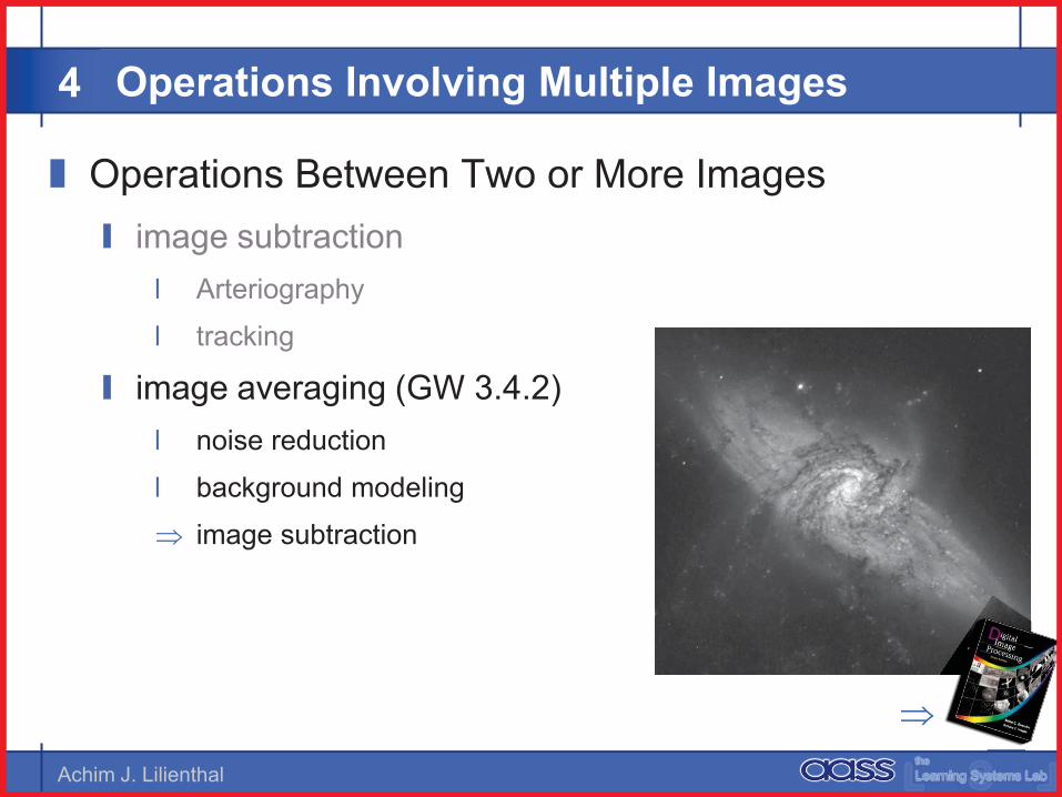
� Operations Between Two or More Images� image subtraction
� Arteriography
� tracking
� image averaging (GW 3.4.2)� noise reduction
� background modeling
� image subtraction
Operations Involving Multiple Images4
�
Achim J. Lilienthal
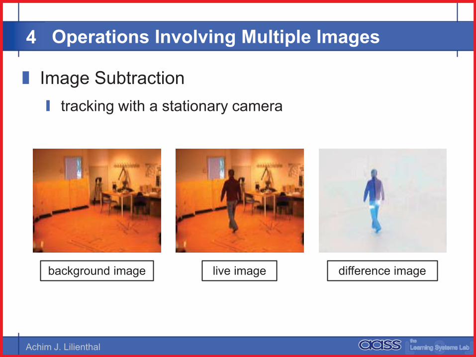
� Image Subtraction� tracking with a stationary camera
Operations Involving Multiple Images4
background image live image difference image
Achim J. Lilienthal
� Operations Between Two or More Images� image subtraction
� Arteriography
� tracking
� image averaging (GW 3.4.2)� noise reduction
� background modeling
� image subtraction
� time constant of averaging ? (stability – plasticity dilemma)� recency weighted averaging
� sample-based background modelling
Operations Involving Multiple Images4
Achim J. Lilienthal
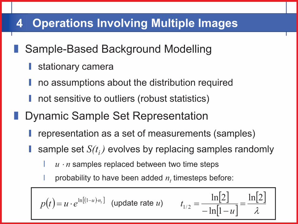
� Sample-Based Background Modelling� stationary camera
� no assumptions about the distribution required
� not sensitive to outliers (robust statistics)
� Dynamic Sample Set Representation� representation as a set of measurements (samples)� sample set S(ti ) evolves by replacing samples randomly
� u � n samples replaced between two time steps
� probability to have been added nt timesteps before:
Operations Involving Multiple Images4
(update rate u)� � � �� �tnueutp ���� 1ln � �� �
� ��2ln
1ln2ln
2/1 ���
�u
t

Achim J. Lilienthal
� Interpretation of a Dynamic Sample Set! dynamic sample sets correspond to a time scale
� Deriving Foreground Probability Images� estimate background distribution
� calculate kernel estimator (Parzen window)
� background probability according to intensity density estimate
� foreground probability = 1 - background probability
Operations Involving Multiple Images4
� � Tcnt ��� 2ln2/1
T
tu c
p �� pu : sample set update probability
�t : time interval since the last frame
ct : time constant

Achim J. Lilienthal
� Foreground Probability Images
Operations Involving Multiple Images4
t1/2 = 1.5 s, � = 20
t1/2 = 115 s, � = 20
Achim J. Lilienthal
IntroductionApplications – People Tracking
� Contents� Contents
Achim J. Lilienthal
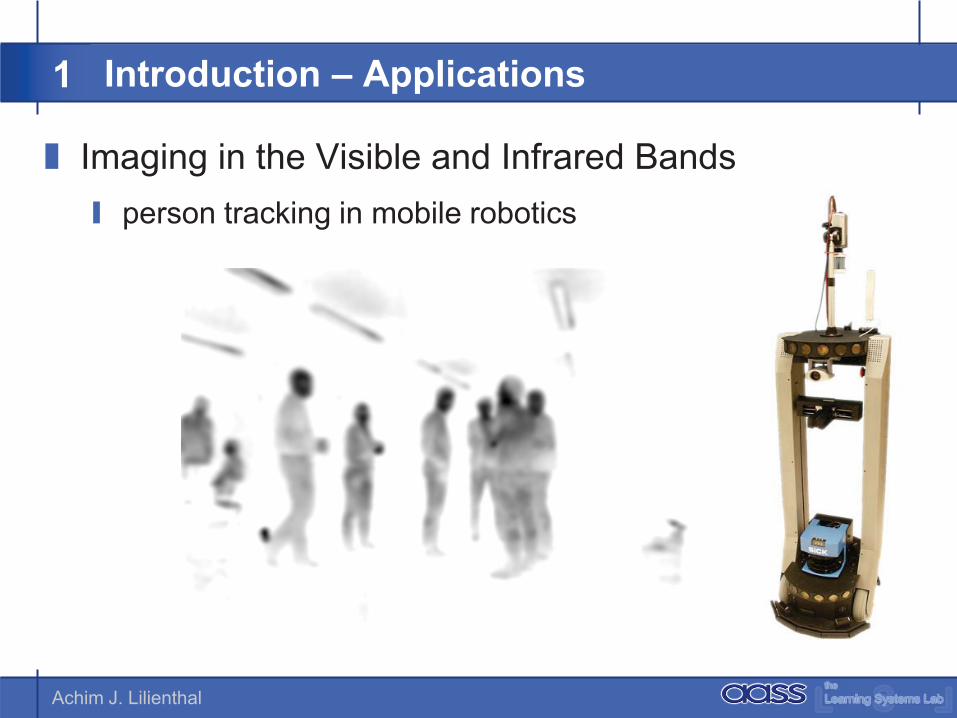
Introduction – Applications1
� Imaging in the Visible and Infrared Bands� person tracking in mobile robotics

Achim J. Lilienthal
Achim J. Lilienthal
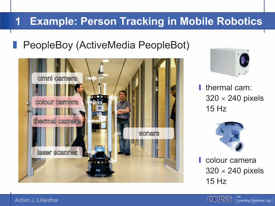
Example: Person Tracking in Mobile Robotics1
� PeopleBoy (ActiveMedia PeopleBot)
� colour camera320 � 240 pixels15 Hz
� thermal cam:320 � 240 pixels15 Hz
Achim J. Lilienthal
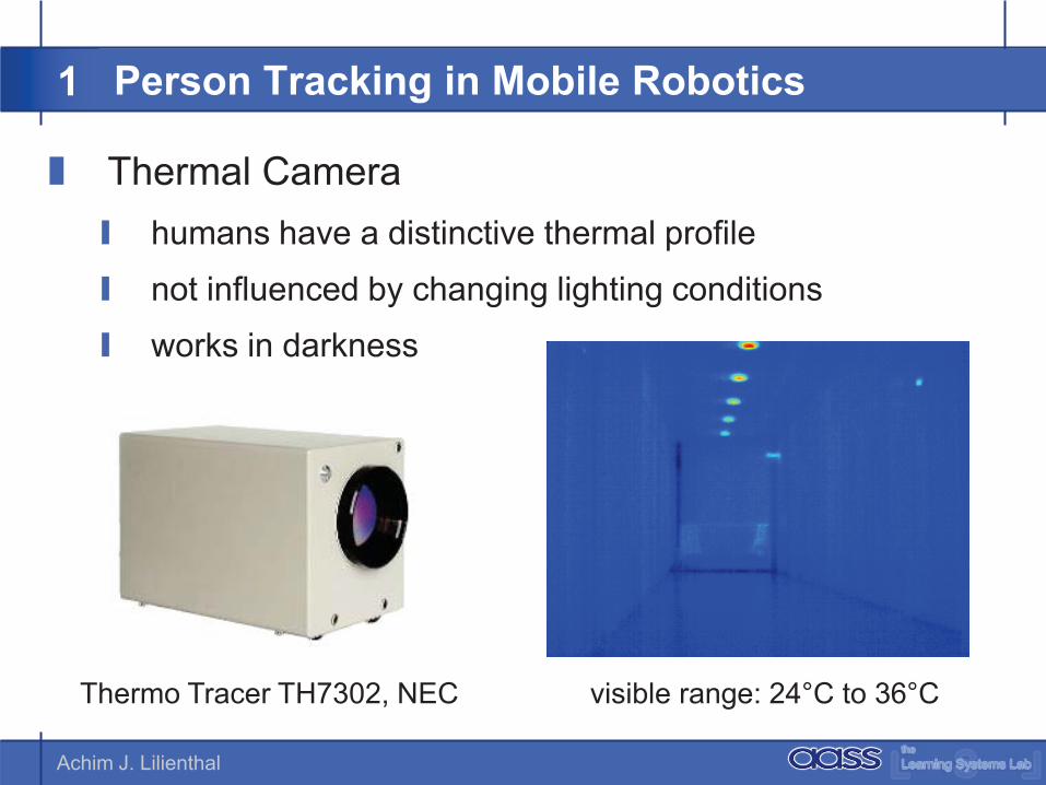
� Thermal Camera� humans have a distinctive thermal profile
� not influenced by changing lighting conditions
� works in darkness
Thermo Tracer TH7302, NEC visible range: 24°C to 36°C
Person Tracking in Mobile Robotics1

Achim J. Lilienthal
� Thermal Camera� humans have a distinctive
thermal profile
� not influenced by changing lighting conditions
� works in darkness
� Colour Camera� improves accuracy
� helps to resolve occlusions� dynamical colour model
Person Tracking in Mobile Robotics1
Achim J. Lilienthal
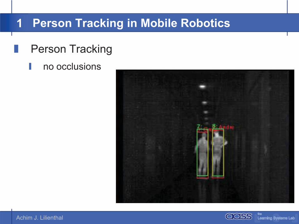
� Person Tracking� no occlusions
Person Tracking in Mobile Robotics1

Achim J. Lilienthal
� Person Tracking� distinguish persons using an elliptic contour model
Person Tracking in Mobile Robotics1
Achim J. Lilienthal
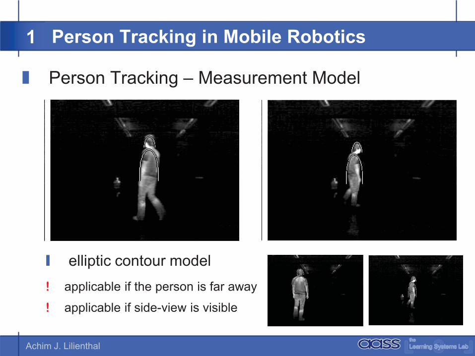
� Person Tracking – Measurement Model
� elliptic contour model
Person Tracking in Mobile Robotics1
! applicable if the person is far away
! applicable if side-view is visible

Achim J. Lilienthal
� Person Tracking� no occlusions
Person Tracking in Mobile Robotics1
Achim J. Lilienthal
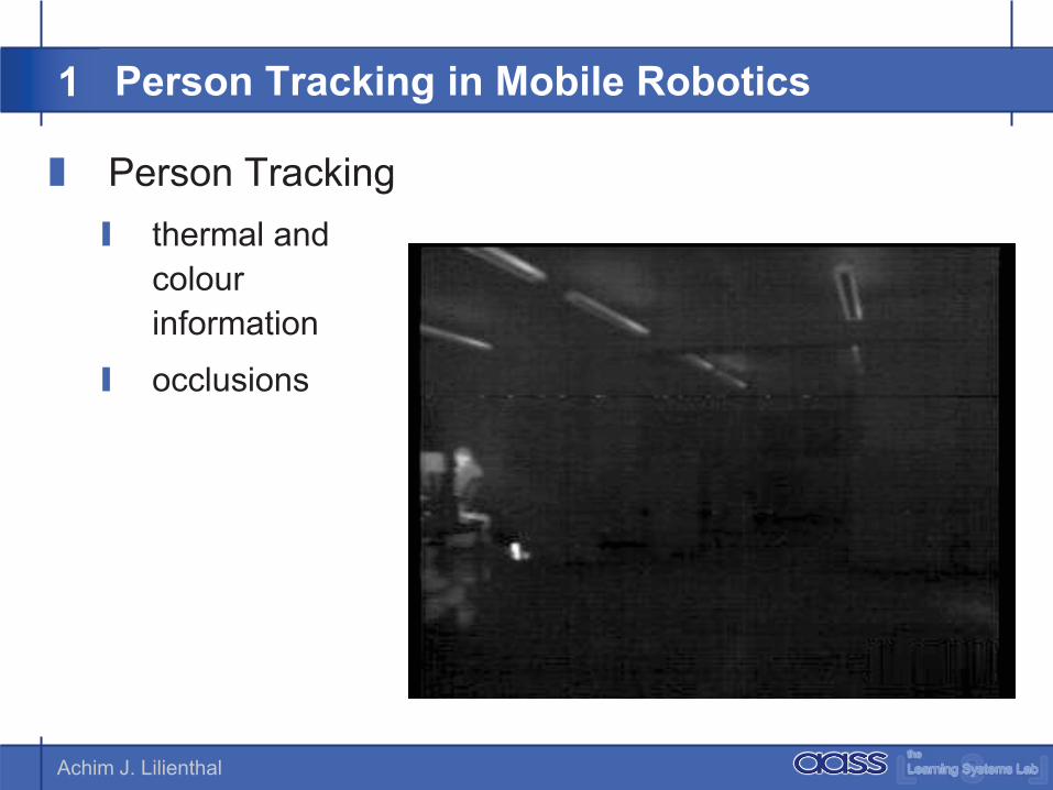
� Person Tracking� thermal and
colour information
� occlusions
Person Tracking in Mobile Robotics1
Achim J. Lilienthal
� Person Tracking� stationary
webcam
� sample-basedbackground subtraction(motion heat)
� occlusions
Person Tracking in Mobile Robotics1