Digital method of spectral peak analysis

I AIDS FOR ANALYTICAL CHEMISTS I Digital Method of Spectral Peak Analysis

Lowell M. Schwartz Unioersity of Massachusetts, Boston, Mass. 021 16

IN APPLICATIONS where quantitative information must be derived from recorded spectra, it is convenient to fit spectral lines with Gaussian or Lorentzian functions (1) and to calcu- late the desired quantities from the function parameters. If y is a measure of the absorption or emission intensity at the position x, Le., the wavelength or frequency in optical spectrometry of the field strength in resonance spectrometry, then a single Gaussian spectral line is expressed as

where the three parameters E, xo , and 6 are the peak height, the position of the center of the peak on the x axis, and the half-width, respectively. The half-width is measured at half the maximum height. In addition to intrinsic interest in these parameters, the area under the entire Gaussian curve can be calculated from them as e61/T/ln 2. The corresponding single Lorentzian spectral line is

y = E [ ( x y ) ’ + 1 1 ‘ 1

and the corresponding area under the curve is ~ e 6 . A difficulty frequently encountered is the overlapping of

several peaks which must be resolved into component lines. This can be done by nonsystematic hand calculation or with the aid of a commercially available electronic device (Model 310 Curve Resolver, E . I. Du Pont de Nemours and Co., Wilmington, Del.). Alternatively, a digital computer method is described in this article. It is particularly well suited to operation from a teletypewriter remote access. The com- putation is based on the principle of least-squares, i .e. , it seeks those Gaussian or Lorentzian parameters which mini- mize the deviation of the computed spectrum from the experimental one.

Theory. In general the least-squares procedure seeks to find particular values of the parameters p I = p l , p ~ , p3, which yield an optimum fit of the function y ( x , p , ) to a set of discrete data y . us. x , in the sense of minimizing the (un- weighted) sum of the squares of the deviations. This is symbolized by

S = Z , b ( x t , p , ) - y J z = minimum ( 3 ) In the conventional least-squares method, the function y ( x , p , ) is a polynomial in x with coefficients p I . This choice of functional form leads to a set of simultaneous algebraic (normal) equations whose solution yields directly the set of least-squares parameters p I . However, a function which is a summation of Gaussian or Lorentzian components results in a set of simultaneous equations which are nonlinear in the unknown p j ’ s and which cannot generally be solved exactly. The means adopted here of circumventing this problem takes advantage of the fact that a crude estimate of the component peaks in a spectrum can usually be made

(1) L. Petrakis, J . Chem. Educ., 44, 432 (1967).

without difficulty. The number of peaks and their approxi- mate heights and positions may be visually apparent, and the widths can be calculated roughly with slightly more effort. Denoting these initially estimated parameters as p j 0 , the method ( 2 ) seeks to find the corrections Apj such that pj = pjo + Apj, In other words, instead of seeking p j directly, the least-squares procedure calculates the set Apj which minimizes

S = z i b ( X i , p j o + Apj) - yiI2 (4) If the estimates p p are good ones, then the corrections will be small and y can be approximated by a truncated Taylor series expansion about p j o :

Y ( x ~ , p i o + P,) MY(xi, ~ 3 ’ ) + z j b ’ i j > A p j ( 5 )

In this expression ( y ’ i , ) = (by /bp j ) are the partial derivatives of y with respect to the parameters p j and are evaluated at each point xi and with p j set at p p . With this approxima- tion, the minimization becomes

(6) If J is the number of component peaks in the spectrum, then taking each (bS/bApj) = 0 yields a set of 3J normal equations in the 3J unknowns. This set can be written concisely in matrix notation as a . A p = b, where the elements of the a and b matrices are, respectively,

and

The indices k and I, like j , refer to component peaks. The vector Ap can be found by matrix inversion methods and yields the set of corrections A p j which when added to the initial estimates p30 provide a refined set of estimates for the next iteration, This procedure is repeated until the calculated corrections become sufficiently small.

It remains to derive expressions for the partial derivatives of the specific Gaussian and Lorentzian functions of interest. For a Gaussian analysis into J peaks,

S = Z , b ( x i , p j o ) + Zj(yij‘)Apj - yiIz = minimum

akz = Z,bt~’ )b iz ’ ) (7)

(8) b~ = Z’iCYit’)IYi - y(xi,pr0))l

and a total of 3J parameters are involved. The derivatives needed for the matrix elements are

~ _ _ _ ~

(2) J. E. Scarborough, “Numerical Mathematical Analysis,” 2nd ed., The Johns Hopkins Press, Baltimore, Md., 1950, p 463.

1336 ANALYTICAL CHEMISTRY, VOL. 43, NO. 10, AUGUST 1971

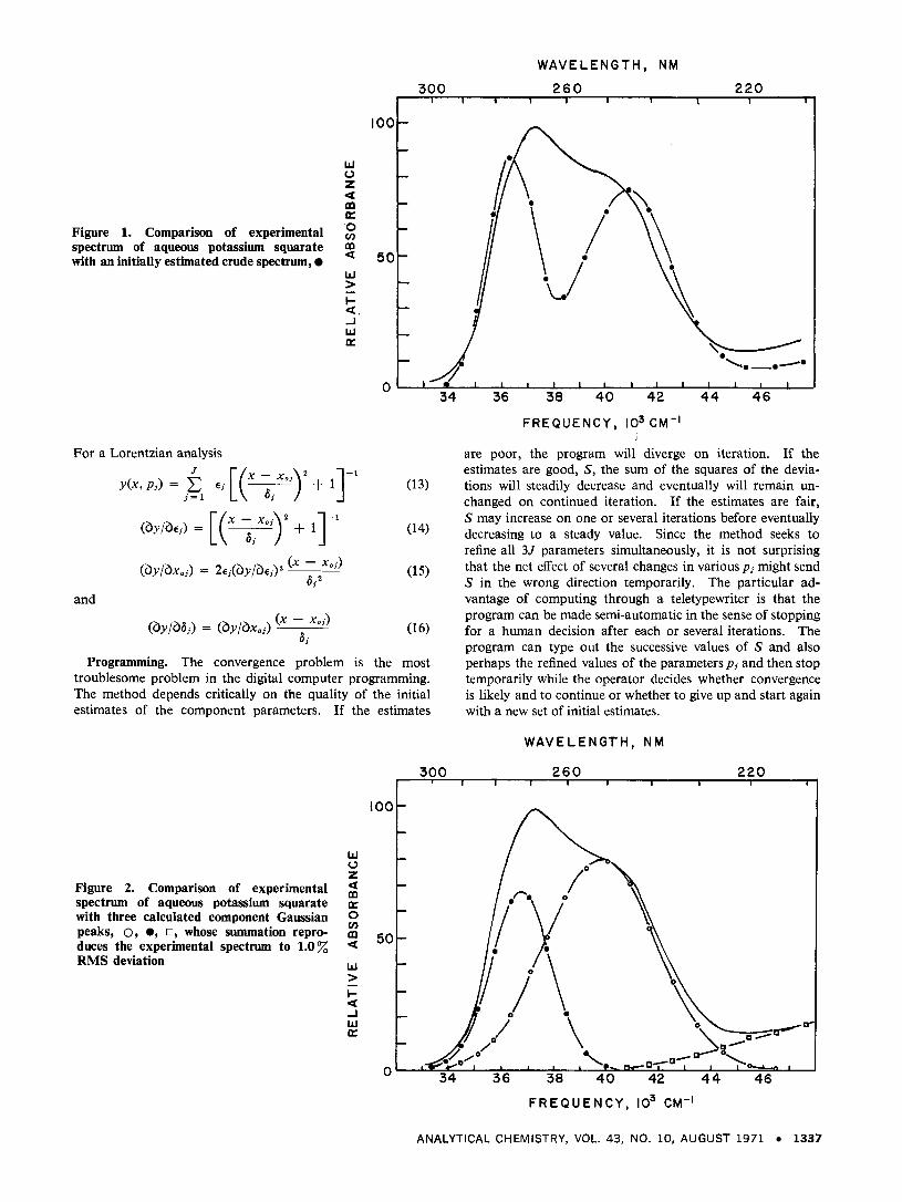
Figure 1. Comparison of experimental spectrum of aqueous potassium squarate with an initially estimated crude spectrum,

For a Lorentzian analysis

W 0 Z

K '0 v)

U

W > c U -I W

a m

m

-

a

WAVELENGTH, NM

300 260 220 I I I 1 1 1 I I I I

Programming. The convergence problem is the most troublesome problem in the digital computer programming. The method depends critically on the quality of the initial

F R E Q U E N C Y , 103 C M - 1

are poor, the program will diverge on iteration. If the estimates are good, S , the sum of the squares of the deviations will steadily decrease and eventually will remain un- changed on continued iteration. If the estimates are fair, S may increase on one or several iterations before eventually decreasing to a steady value. Since the method seeks to refine all 3J parameters simultaneously, it is not surprising that the net effect of several changes in various p j might send S in the wrong direction temporarily. The particular advantage of computing through a teletypewriter is that the program can be made semi-automatic in the sense of stopping for a human decision after each or several iterations. The program can type out the successive values of S and also perhaps the refined values of the parameters p , and then stop temporarily while the operator decides whether convergence is likely and to continue or whether to give up and start again

estimates of the component parameters. If the estimates with a new set of initial estimates.

W A V E L E N G T H , N M

300 2 6 0 220 I I I I I I I 1 I

100 - -

w - 0 z

Figure 2. Comparison of experimental 2 spectrum of aqueous potassium squarate a with three calculated component Gaussian peaks, 0, 0, n, whose summation repro- 2 duces the experimental spectrum to 1.0

w RMS deviation > c U J w

- -

- - - -

-

a

I , ,

34 36 38 40 42 44 46 0

F R E Q U E N C Y , io3 C M - 1

ANALYTICAL CHEMISTRY, VOL. 43, NO. 10, AUGUST 1971 1337

If the program diverges, one method is to improve the set of initial estimates and perhaps add more component peaks to the summation. An alternative remedy is to reduce the magnitudes of corrections before adding them to the parameters. For example, if all the corrections are reduced by a factor of ten and if the set of parameters is divergent, the ad- verse effect on S will be reduced by about a factor of ten and the calculation may recover on subsequent iterations. The price paid for this improved chance of convergence is that the convergence itself takes that many more iterations.

Sample Results. A program has been written in FORTRAN for use on the time-sharing system of the CDC 3600 computer at the University of Massachusetts at Amherst through a teletypewriter linkage to the University of Massachusetts at Boston. (Program listing is available on request.) The program analyzes for a maximum of four Gaussian components. The analysis of an experimental ultraviolet spectrum of potassium squarate is shown in Figures 1 and 2. Although previously published by Ireland and Walton (3),

(3) D. T. Ireland and H. F. Walton, J. Phys. Chem., 71, 751 (1967).

this spectrum was reproduced in this laboratory using a Cary 14 spectrophotometer. A fairly poor estimate of the parameters of three Gaussian components is as follows:

Com- ponent € xo, lo3 cm-1 6, IOa cm-1

1 85 36.4 1 .06 2 74 40.8 2.00 3 50 62.5 9.17

These components sum up to the crude spectrum shown in Figure 1. Eventually the least-squares iterative calculation converged to the folldwing set of parameters :

Com- ponent E XO 6

1 67 .7 36.8 1 .33 2 80.1 39.8 2.48 3 18.4 48.4 3.97

and the corresponding component peaks are shown in Figure 2. The summation of these peaks approximates the experimental spectrum with an average (RMS) deviation of 1.0%.

RECEIVED for review March 4,1971. Accepted May 25,1971.

Solid State Pressure Transducer for Pressuremetric Titrations

D. J. Curran and S. J. Swarin Department of Chemistry, University of Massachusetts, Amherst, Mass. 01002

A NUMBER OF REACTIONS of interest in analytical chemistry involve gases. Therefore the measurement of changes in the amount of gas present, particularly at the micromolar level, is of interest. In a recent paper ( I ) , we pointed out specific areas of application of this measurement technique and presented an electronic conductivity manometer for use in this field. Quinn and Posipanko (2) have demonstrated the use of a solid state pressure transducer called a Pitran (for Piezotransistor) (Stow Laboratories, Inc., Hudson, Mass. 01749) for monitoring the course of chemical reactions in a closed-system. As part of our studies of applications of pressure transducers in chemical analysis, we have undertaken a study of this unique device to determine its usefulness for the measurement of small pressure changes in reactions of analytical interest.

Most transducers for the conversion of pressure to an electrical signal involve a variable but passive electronic circuit element such as a resistor, capacitor, or inductor. The Pitran is unique because it is the first transducer that involves an active circuit element. It is a silicon planar NPN transistor with a stress sensitive emitter-base junction. Pres- sure applied to the front side of the top of the transistor header produces a large reversible change in the gain of the transistor, i .e., the Pitran output is modulated by the mechanical variable. Holes in the physical base of the transistor permit access of the prevailing atmospheric pressure (or a set reference pressure) to the back side of the top of the transistor header. Thus the transistor header is a diaphragm responding to the difference in pressure between its front and back sides; and the output of the device is differential.

(1) D. J. Curran and S. J. Swarin, ANAL. CHEM., 43, 358 (1971). (2) E. L. Quinn and T. Posipanko, Reu. Sei. Instrum., 41, 475

(1970).

When the device is connected in a simple common emitter configuration (Figure l), it provides a dc output proportional to the mechanical input.

The Pitran appears to have application in the areas we have cited previously: reaction kinetics, null point pres- suremetry, and pressuremetric titrations ( I ) . We have demonstrated here the applicability of this instrument as an end-point detection device in pressuremetric titrations of 1,904- and 0.8694-mg samples of ammonium ion with elec- trogenerated hypobromite. Nitrogen is produced according to the following equations:

(1) Br- + 20H- + BrO- + HzO + 2e-

2NH4+ + 3Br0- + Nzt + 3Br- + 2H+ + 3Hz0 (2)

EXPERIMENTAL

Apparatus. The complete circuit diagram of the pressure transducer system is given in Figure 1. All of the components except the Pitran were mounted in a 51/4 X 3 X 2l/*- inch aluminum chassis. The power supply was a nine-volt transistor battery. The Pitran was mounted as shown in Figure 2. Since the Pitran is mounted to fit into the transistor socket, it was connected to the circuitry by simply fastening the 18/9 ball and socket joints together.

The Pitran used in this study was a Model PT-M2 which has a nominal linear pressure range of 0.25 psid. Pressure signals for testing the linearity and reproducibility of the transducer were supplied by a hydrogen-nitrogen coulometer designed according to the recommendations of Page and Lingane (3) and operated with a Sargent Model IV Constant Current Source. The recorder, constant temperature bath, submersible magnetic stirring motor, potentiometer, Ampot,

(3) J. A. Page and J. J. Lingane, Anal. Chim. Acta., 16, 175 (1957).

1338 ANALYTICAL CHEMISTRY, VOL. 43, NO. 10, AUGUST 1971

Documents

Digital method of spectral peak analysis