Digital Signal Processing 48 (2016) 163–177

Contents lists available at ScienceDirect

Digital Signal Processing

www.elsevier.com/locate/dsp

Performance analysis of a family of adaptive blind equalization

algorithms for square-QAM

Ali W. Azim a,b, Shafayat Abrar c,∗, Azzedine Zerguine d, Asoke K. Nandi e

a Institute Polytechnique de Grenoble Saint Martin d’Hères, 38400, Franceb COMSATS Institute of Information Technology, Wah Cantt 47040, Pakistanc COMSATS Institute of Information Technology, Islamabad 44000, Pakistand King Fahd University of Petroleum & Minerals, Dhahran 31261, Saudi Arabiae Brunel University London, Uxbridge, Middlesex UB8 3PH, United Kingdom

a r t i c l e i n f o a b s t r a c t

Article history:Available online 25 September 2015

Keywords:Multimodulus algorithmBlind equalizationAdaptive equalizersSteady-state analysisReceiver designConvergence analysis

Multimodulus algorithms (MMA) based adaptive blind equalizers mitigate inter-symbol interference and recover carrier-phase in communication systems by minimizing dispersion in the in-phase and quadrature components of the received signal using the respective components of the equalized sequence in a decoupled manner. These equalizers are mostly incorporated in bandwidth-efficient digital receivers which rely on quadrature amplitude modulation (QAM) signaling. The nonlinearities in the update equations of these equalizers tend to lead to difficulties in the study of their steady-state performance. This paper presents originally the steady-state excess mean-square-error (EMSE) analysis of different members of multimodulus equalizers MMAp–q in a non-stationary environment using energy conservation arguments, and thus bypassing the need for working directly with the weight error covariance matrix. In doing so, the exact and approximate expressions for the steady-state mean-square-error of several MMA based blind equalization algorithms are derived, including MMA2–2, MMA2–1, MMA1–2, and MMA1–1. The accuracy of the derived analytical results is validated using Monte–Carloexperiments and found to be in close agreement.

© 2015 The Authors. Published by Elsevier Inc. This is an open access article under the CC BY license (http://creativecommons.org/licenses/by/4.0/).

1. Introduction

Blind equalizers mitigate different types of interferences such as inter-symbol interference (ISI), frequency selective fading, etc., caused by non-ideal transformations performed by the dispersive channels in a communication system. A blind adaptive equalizer attempts to compensate for the distortions of the channel by pro-cessing the received signals and reconstructing the transmitted sig-nal up to some indeterminacies by the use of linear or nonlinear filters without any knowledge of the channel impulse response and without direct access to the transmitted sequence itself. The basic idea behind an adaptive blind equalizer is to minimize or maxi-mize some admissible blind objective or cost function through the choice of filter coefficients based on the equalizer output [1–3].

* Corresponding author. Fax: +92-336-232-1845.E-mail addresses: ali-waqar.azim@ensimag.grenoble-inp.fr,

aliwaqar@ciitwah.edu.pk (A.W. Azim), sabrar@comsats.edu.pk (S. Abrar), azzedine@kfupm.edu.sa (A. Zerguine), asoke.nandi@brunel.ac.uk (A.K. Nandi).

http://dx.doi.org/10.1016/j.dsp.2015.09.0021051-2004/© 2015 The Authors. Published by Elsevier Inc. This is an open access article

The performance of an adaptive filter can be evaluated using transient and steady-state analyses. The former provides informa-tion about the stability and the convergence rate of an adaptive filter, whereas the latter provides information about the mean-square-error of the filter once it reaches steady state. In the steady-state analysis of adaptive filters, one of the properties to be con-sidered is their ability to track changes/variations in the signal statistics of the received signal. This property is of significant im-portance, particularly in mobile communications systems and ap-plications like acoustic echo cancellation, etc.

Blind adaptive filters (or equalizers) are based on recursive al-gorithms that allow the filter to adapt and track (slow) variations in input statistics. Such adaptive filters start from certain initial conditions without any prior knowledge about the input signal statistics, then the filter coefficients are updated based on the cho-sen adaptive algorithms and the sequence of the sampled data values. In stationary environments, adaptive filters converge to op-timum Wiener solution [4–13]. However, in non-stationary envi-ronments, the optimum Wiener solution takes time-varying form that results in variation of saddle point in error performance sur-

under the CC BY license (http://creativecommons.org/licenses/by/4.0/).

164 A.W. Azim et al. / Digital Signal Processing 48 (2016) 163–177

face and consequently affecting the performance of filters, thus, tracking the variations in underlying signal statistics is consid-ered to be a useful and important property for adaptive filters. These variations in underlying signal statistics and consequently saddle point can be tracked by using tracking performance analysis. The performance metric to be considered for tracking performance of an adaptive filter is the steady-state excess mean-square-error (EMSE). The EMSE can be defined as the difference between the mean-square-error (MSE) of the filter in steady-state and its mini-mum value. The smaller the EMSE of an adaptive filter, the better it is [14]. If filter parameters (like step-size) are chosen correctly, the filter can track variations in underlying signal statistics. How-ever, tracking fast variations might prove to be a challenging task or at times impossible to perform [14].

The widely adopted adaptive blind equalization algorithm is the so-called Constant Modulus Algorithm (CMA2–2) [2,15–17]. For quadrature amplitude modulation (QAM) signaling, however, a tai-lored version of CMA2–2, commonly known as Multimodulus Al-gorithm (MMA2–2) is considered more suitable. The MMA2–2 is capable of jointly achieving blind equalization and carrier phase recovery, whereas the CMA2–2 requires a separate phase-lock loop for achieving carrier phase recovery. The family of MMA, MMAp–q, is associated with the minimization of the dispersion-directed cost-function with two degrees of freedom. By selecting appro-priate values of p and q, the generic split cost-function leads to the respective cost-functions of several existing blind equalization algorithms [18–21]. Interested readers are referred to [22] for de-tailed discussion on MMAp–q. The update expressions of these algorithms are inherently nonlinear in nature due to the presence of nonlinear error-functions [20,23–27].

Algorithms like CMA2–2/MMA2–2 have recently been employed in optical systems for polarization mode demultiplexing and also to mitigate the effects of other types of interferences like chro-matic and polarization mode dispersions in optical systems. Since 2008 [28], CMA2–2 and its variants have become the most exper-imented algorithms for blind polarization demultiplexing [29–36]. In [37], authors have compared CMA2–2 with an independent component analysis (ICA) based algorithm to demultiplex the polarization adaptively. Recently in [38–43], authors have used MMA2–2 and its variants as a joint adaptive solution for blind de-multiplexing and carrier phase recovery in coherent optical system. Afterwards, βMMA (which is an optimized version of MMA2–1) [44] has been employed in coherent optical receiver to demulti-plex polarization mode signals adaptively [45].

In this paper, the approach that has been adopted for steady-state tracking analysis of multimodulus equalizers exploits the study of energy propagation through each iteration of an adaptive filter using a feedback structure (which consists of a lossless feed-forward block and a feedback path), and it relies on energy con-servation arguments [14]. The convenience of this approach is that it allows us to avoid working with nonlinear update equations and thus bypasses the need for working directly with the weight error covariance matrix. In particular, using the fundamental variance relation arguments, we derive expressions for steady-state EMSE of MMA2–2, MMA2–1, MMA1–2 and MMA1–1 under the assump-tion that the quadrature components of the successfully equalized signal are Gaussian distributed when conditioned on true signal al-phabets. Our objective is not to study the conditions under which an algorithm will tend to converge successfully, rather to evaluate its expected steady-state performance once it has converged suc-cessfully.

1.1. Literature review

The nonlinearity of most of the adaptive equalizers, includ-ing CMA2–2 and MMA2–2, makes the steady-state analysis and

tracking performance a difficult task to perform. As a result, only a handful of results is available in the literature concerning the steady-state performance of adaptive equalizers. A few results are available on EMSE analysis of CMA2–2 like Fijalkow et al. [46]employed ingenious use of Lyapunov stability and averaging anal-ysis, Shynk et al. [47] used Gaussian regression vector assumption, and some exploited the variance relation theorem [48,49] to eval-uate the same. Steady-state analyses of adaptive filters have gained interest due to their ease in analysis. Recently, Abrar et al. [50] per-formed the EMSE analysis of CMA2–2 and βCMA [51] by assuming that the modulus of equalized signals are Rician distributed in the steady-state. In a recent work [52], we have performed the EMSE analysis of MMA2–2 and βMMA [44] by assuming that the real and imaginary parts of equalized signals are Gaussian dis-tributed in the steady-state. Moreover, the approach of [14] has been employed to study the steady-state performance of a num-ber of adaptive blind equalization algorithms e.g., the so-called hybrid algorithm [53], the square contour algorithm [54], the im-proved square contour algorithm [55], and the varying-modulus algorithms [56].

1.2. Notation

Unless otherwise mentioned, scalars are represented by italic letters (e.g., K ). Lower-case boldface letters are used to denote vectors and upper-case boldface letters are associated with matri-ces, e.g., w and R , respectively. In addition, the symbol ⊗ and operators (·)∗ , (·)T and (·)H respectively represents the convo-lution operation, complex conjugate operator, transpose operator and Hermitian (conjugate transpose) operator. The operator ‖ · ‖when applied to a vector gives the Euclidean norm of the vec-tor, whereas, the operator | · | gives the absolute vector. Further, E, �[·] and I denotes the expectation operator, the real part of the complex entity, and identity matrix of appropriate dimen-sions, respectively. The operator Tr(·) gives the trace of the ma-trix.

1.3. Paper organization

The paper is organized as follows: In Section 2, we describe the mathematical model for the system. Section 3 provides a brief introduction of different members of MMA family that we aim to discuss here. Section 4 introduces the non-stationary environ-ment and the framework for EMSE analyses. Section 5 presents the analytical expressions evaluated for steady-state tracking per-formance analysis for MMA2–2, MMA2–1, MMA1–2 and MMA1–1equalizers. Section 6 compares the proposed approach with ex-isting state-of-the-art methods. Section 7 provides a number of computer simulations on steady-state tracking performance analy-sis of the algorithms considering different scenarios: for equalized zero-forcing solution, equalizing a time-varying channel, studying the effect of filter-length on EMSE on a time-invariant channel, and adaptive optical demultiplexing in a coherent optical system. In addition, it also compares the theoretical results predicted by our expressions with the simulated values. Finally, Section 8 draws conclusions.

2. System model

Fig. 1 depicts a typical baseband communication system. Consider that the channel response is given by a K -tap vector hn = [hn,0, hn,1, · · · , hn,K−1], then the full rank (N + K − 1) × Nchannel convolution matrix H is given by following Toeplitzmatrix

A.W. Azim et al. / Digital Signal Processing 48 (2016) 163–177 165

Fig. 1. A typical baseband communication system.

H =

⎡⎢⎢⎢⎢⎢⎢⎢⎢⎢⎢⎢⎢⎣

hn,0 0 · · · 0 · · ·hn,1 hn,0

. . . 0. . .

... hn,1. . .

.... . .

hn,K−1...

. . . hn,0. . .

0 hn,K−1. . . hn,1

. . .

...... · · · . . .

. . .

⎤⎥⎥⎥⎥⎥⎥⎥⎥⎥⎥⎥⎥⎦

(1)

The received signal xn is the convolution of transmitted se-quence {an} = [an, an−1, · · · , an−K+1]T and channel impulse re-sponse hn as given by xn = hT

n an; the sequence {an} is indepen-dent and identically distributed (i.i.d.), and takes values of equally likely square-QAM symbols. The vector xn is fed to the equalizer to combat the interference introduced by the propagation channel and estimate delayed version of the transmitted sequence {an−δ}, where δ denotes delay parameter.

Let wn = [wn,0, wn,1, · · · , wn,N−1]T be the impulse response of equalizer and xn = [xn, xn−1, · · · , xn−N+1]T be the vector of chan-nel observations (the regressor vector) with input covariance ma-trix R = ExnxH

n , where N is the number of equalizer taps. The output of equalizer is the convolution of regression vector and equalizer impulse response is given as yn = w H

n−1xn . Let tn =hn ⊗ w∗

n−1 be the overall channel-equalizer impulse response. Us-ing (1), we obtain tn = hn ⊗ w∗

n−1 = Hw∗n−1. Under successful

convergence, we have tn = e is ideally single-spike where e =[0, · · · , 0, 1, 0, · · · , 0]T .

A generic stochastic gradient-based adaptive equalizer for which the updating algorithm is given as [14]

wn = wn−1 + μϕ(yn)∗xn (2)

where μ is a small positive step-size, governing the speed of con-vergence and the level of steady-state equalizer performance, and ϕ(yn) is complex-valued error function. For multimodulus equal-izers, the error function is non-analytic in nature, i.e., it is a de-coupled function of the quadrature components of deconvolved sequence yn , which is expressed as

ϕ(yn) = ψ(yR,n) + jψ(yI,n), (3)

so that the real and imaginary parts of ϕ(yn) are obtained from the real yR,n and imaginary parts yI,n of yn , respectively.

3. The multimodulus equalizers

The Multimodulus Algorithm (MMA) is considered more suitable for QAM signaling. A generalized dispersion-directed (split) cost-function of generic MMAp–q equalizers is given as follows [22]:

J MMAp–q = E∣∣|yR,n|p − R p

R

∣∣q + E∣∣|yI,n|p − R p

I

∣∣q (4)

where p and q are positive integers, and R R and R I are disper-sion constants chosen in accordance with the source statistics in order to guarantee that the global minima of J MMAp–q occurs at zero-forcing solutions. The cost function defined in (4) can be con-sidered as a generalization of Wesolowski’s cost-function [23] with

two degrees of freedom or the split version of Larimore and Treich-ler (CM) cost-function [57]. The corresponding stochastic gradient-based adaptive algorithm is [22]

wn = wn−1 + μ[∣∣|yp

R,n| − R pR

∣∣q−2|yp−2R,n |

(R p

R − |ypR,n|)

yR,n

+ j∣∣|yp

I,n| − R pI

∣∣q−2|yp−2I,n |

(R p

I − |ypI,n|)

yI,n

]∗xn (5)

A multitude of algorithms can be obtained for different choices of p and q, providing a possible flexibility in the design of blind equalizers. In the sequel, the algorithm defined by recursion (5) is referred as MMAp–q and for the sake of simplicity, we will use subscript L to denote either R or I . Expression (5) generalizes a number of existing blind adaptive equalization algorithms. Among them, these are the following:

1. For p = q = 2, (4) reduces to following split cost function which was proposed independently by Wesolowski [19], Oh and Chin [20] and Yang et al. [24]:

J MMA2–2 = minw

{E(

y2R,n − R2

R

)2 + E(

y2I,n − R2

I

)2}

(6)

where R2L = Ea4

L/Ea2L . The tap weight vector of MMA2–2 is up-

dated according to

wn = wn−1 + μ[(R2

R − y2R,n)yR,n + j(R2

I − y2I,n)yI,n

]∗xn

(7)

2. For p = 2 and q = 1, (4) results in MMA2–1 equalization algo-rithm that employs the following cost function1

J MMA2–1 = minw

{E∣∣∣y2

R,n − R2R

∣∣∣+ E∣∣∣y2

I,n − R2I

∣∣∣} (8)

The tap weight vector of MMA2–1 is updated to minimize (8)using a gradient-descent adjustment algorithm according to

wn = wn−1 + μ[sgn(

R2R − y2

R,n

)yR,n

+ j sgn(

R2I − y2

I,n

)yI,n]∗

xn (9)

3. For p = 1, q = 2, (4) reduces to an equivalent form of Benveniste–Goursat cost–function [18]. We denote the result-ing algorithm as MMA1–2, and ultimately (4) results in

J MMA1–2 = minw

{E(|yR,n| − R R

)2 + E(|yI,n| − R I

)2} (10)

where R L = Ea2L/E|aL |. The tap weight vector of MMA1–2 is

updated to minimize (10) using a gradient-descent adjustment algorithm according to

wn = wn−1 + μ[(

R R sgn(yR,n) − yR,n)

+ j(

R I sgn (yI,n) − yI,n)]∗

xn (11)

4. For p = q = 1, (4) reduces to an equivalent form of the cost-function independently proposed by Weerackody et al. in 1991 [58] and Im et al. in 2001 [21]. We denote the resulting algo-rithm as MMA1–1 and its cost function is given as follows2:

1 In MMA2–1, the dispersion constant RL is obtained as RL = 2�z� − 1, where �z� is the smallest positive integer greater than or equal to z [22]. The parameter z is given by z = (z1/12) + (1/z1) where z1 is given as 3

√108z2 + 12

√81z2

2 − 12, z2 = 0.5

√M(M − 1) and M denotes the size of constellation. It gives RL = 3, 7, and

13 for 16-, 64-, and 256-QAM, respectively.2 The dispersion constant RL for MMA1–1 is given as RL = 2�z� − 1 [22]. For

M-point constellation we have z = √M/8 which gives RL = 3, 5, and 11 for 16-,

64-, and 256-QAM, respectively.

166 A.W. Azim et al. / Digital Signal Processing 48 (2016) 163–177

J MMA1–1 = minw

{E∣∣|yR,n| − R R

∣∣+ E∣∣|yI,n| − R I

∣∣} (12)

The tap weight vector of MMA1–1 is updated to minimize (12)using a gradient-descent adjustment algorithm according to

wn = wn−1 + μ[sgn(

R R sgn(yR,n) − yR,n)

+ j sgn(

R I sgn(yI,n) − yI,n)]∗

xn (13)

4. Non-stationary environment and energy conservation relation

We consider a non-stationary system model in which the vari-ations in the Wiener solution, wo , follow usually a first-order ran-dom walk model [14]:

won = wo

n−1 + qn (14)

where the random vector qn is an i.i.d. zero-mean random vector with positive definite covariance matrix given as Q =EqnqH

n = σ 2q I . We assume that qn is independent of both {am} and

{xm, wo−1} for all m < n [14]. Using the time-dependent Wiener solution, the desired data an can be expressed as

an = (won−1)

H xn + ϑn, (15)

where ϑn is the measurement or gradient noise and is uncorre-lated with xn , i.e., Eϑ∗

n xn = 0 [59]. Defining the weight error vector w̃n as w̃n := wo

n − wn , (2), for a non-stationary environment is expressed as

w̃n = w̃n−1 − μϕ(yn)∗xn + qn (16)

Defining the so-called a priori and a posteriori estimation errors as ea,n := w̃ H

n−1xn and ep,n := (w̃n − qn)H xn , respectively. We can rewrite (16) in terms of the error measures {w̃n, w̃n−1, ea,n, ep,n}alone. For this purpose, we note that if we multiply (16) by xn

from the right, we find that the a priori and a posteriori estimation errors {ea,n, ep,n} are related via

ea,n = ep,n + μ‖xn‖2ϕ(yn) (17)

Relation (17) reveals that ea,n depends on channel variation, adap-tion, and gradient noise. Thus, the steady-state EMSE and the tracking performance of an adaptive equalizer can be quantified by the energy of ea,n . From (17), we can associate the error-function of an equalizer with the a priori and the a posteriori estimation er-rors as follows:

ϕ(yn) = ea,n − ep,n

μ‖xn‖2(18)

Substituting (18) in (16) and rearranging the terms, we obtain the energy conservation relation

‖w̃n‖2 + |ea,n|2‖xn‖2

= ‖w̃n−1‖2 + |ep,n|2‖xn‖2

(19)

It is important to note that (19) holds for any adaptive algorithm. Fig. 2 represents the physical interpretation of (19) which links the energies of the weight error vector as well as the a priori and the a posteriori estimation errors by stating that mapping from the vari-ables

{w̃n−1, ep,n/‖xn‖} to the variables

{w̃n, ea,n/‖xn‖} is energy

preserving. The relation (19) characterizes the energy preserving property of the feed-forward path, whereas the relation (17) char-acterizes the feedback path. The function M denotes the mapping between the two variables and z−1 denotes the unit delay opera-tor. Substituting the expression of ep,n from (17) into (19), we get the fundamental variance relation theorem.

Fig. 2. Lossless mapping and feedback loop.

Theorem 1 (Variance relation). (See [14].) Consider any adaptive fil-ter of the form (2), and assume filter operation in steady-state. Assume further that an = (wo

n−1)H xn + ϑn, where wo

n−1 varies according to the random-walk model (14), where qn is a zero-mean i.i.d. sequence with covariance matrix Q . Moreover, qn is independent of {am} and {xm, wo−1} for all m < n. With yn = an − ea,n, it is true that

2E� [e∗a,nϕ(yn)

]= μTr(R)E|ϕ(yn)|2 + μ−1Tr( Q ) (T1.1)

Expression (T1.1) can be solved for steady-state EMSE, which is defined as

EMSE � limn→∞ E|ea,n|2 (20)

The procedure of evaluating EMSE using (T1.1) avoids the need for explicit evaluation of E‖w̃n‖2 or its steady-state value E‖w̃∞‖2

which can be a burden especially for adaptive schemes with non-linear update equations. In the sequel, in addition to the variance relation, the following justified assumptions are used:

A1) In steady-state the a priori estimation error ea,n is independent of both the transmitted sequence {an} and the regressor vector xn [14].

A2) The number of filter taps is large enough so that by virtue of the central limit theorem, ea,n is zero-mean complex valued Gaussian [59,60].

A3) The optimum filter achieves perfect equalization (zero-forcing solution) an ≈ (wo

n−1)H xn; however, due to channel variation

and gradient noise, the equalizer weight vector is not equal to wo

n even in steady-state [61]. Additionally, no additive noise is assumed in the system (see [48,49,62–67]).

Assumption A1 is the orthogonality condition required for a suc-cessful convergence. Assumption A2, the Gaussianity of a prioriestimation error, has appeared in a number of recent publications. For example, Bellini [68] discussed that the convolutional noise (which bears similar mathematical definition as that of a prioriestimation error) may be considered as zero-mean Gaussian. More-over, [69] discussed that the a priori estimation error (for a long equalizer) may be modeled as a zero-mean Gaussian random vari-able. It has been shown that the steady-state a priori estimation error is zero-mean Gaussian, even for the case where the measure-ment noise is taken to be uniformly distributed. The assumptionA3 is based on the understanding that CMA2–2 and similarly its multimodulus variants diverge on infinite time horizon when noise is unbounded. Interested readers may refer to [70] for a detailed discussion on this issue. Note that the (total) mean square error, MSE of a non-diverging equalizer in the presence of additive noise, however, can always be given as MSE = σ 2

ϑ + EMSE, where σ 2ϑ is

the variance of modeling error/measurement noise. The degree of non-stationarity (DN) of the data is defined as DN �

√Tr(R Q )/σ 2

ϑ

[14]. DN > 1 means that the statistical variations in the optimal weight vector are too fast for the filter to track them. However, if DN � 1, then the filter would generally be able to track the varia-tions in weight vector [14].

A.W. Azim et al. / Digital Signal Processing 48 (2016) 163–177 167

Here onwards, for the sake of notational simplicity, we use ζ :=EMSE, ea := ea,n , y := yn , a := an , ϕ := ϕ(yn) and Pa = E|a|2 =E(a2

R + a2I ). Also, the acronyms LHS and RHS are used to denote

the left-hand side and the right-hand side, respectively.

5. Steady-state EMSE analysis

We now apply the fundamental variance relation to differ-ent MMA adaptive algorithms to obtain analytical expressions for steady-state EMSE by evaluating the energy of error-function as well as its correlation with a priori estimation error. Due to space limitations, we omit some trivial details and only highlight the main steps in the arguments.

5.1. The EMSE of MMA2–2 equalizer

Using the fundamental variance relation (T1.1), we have the fol-lowing theorem for the tracking EMSE of MMA2–2 equalizer:

Theorem 2 (Tracking EMSE of MMA2–2). Consider the MMA2–2 recur-sion (7) with complex-valued data. Consider the non-stationary model (14) with a sufficiently small degree of non-stationarity. Then its EMSE can be approximated by the following expression for a sufficiently small step-size μ:

ζ MMA2–2(μ) = μc1 + 1μ Tr( Q )

c2 − μc3, (T2.1)

μMMA2–2opt =

√Tr( Q )c1c2

2 + Tr( Q )2c23 − Tr( Q )c3

c1c2

with ζ MMA2–2min = 2Tr( Q )

μoptc2(T2.2)

where, c1 := 2Tr(R)(Ea6

R − 2R2R Ea4

R + R4R Ea2

R

), c2 := 2(3Ea2

R − R2R),

and c3 := Tr(R)(3Ea4

R + R4R

). Substituting the expression for μopt into

the expression of EMSE we find the corresponding optimal EMSE.

Proof. In [52], we obtained the following polynomial for EMSE of MMA2–2:

154 ζ 3μTr(R) + ζ 2

(μTr(R)

(452 Ea2

R − 3R2R

)− 3

)

− ζ

(6Ea2

R − 2R2R − μTr(R)

(3Ea4

R + R4R

))

+ μTr(R)

(2Ea6

R + 2R4R Ea2

R − 4R2R Ea4

R

)+ μ−1Tr( Q ) = 0 (21)

In order to evaluate some closed-form expressions of ζ MMA2–2, cer-tain approximations have to be made, e.g., by neglecting the cubic and quadratic terms in (21), we obtain

ζ

(μTr(R)(3Ea4

R + R4R) − 6Ea2

R + 2R2R

)

+ μTr(R)

(2Ea6

R + 2R4R Ea2

R − 4R2R Ea4

R

)+ μ−1Tr( Q ) = 0 (22)

which yields the following closed-form solution:

ζ MMA2–2 = μ2Tr(R)(2Ea6

R + 2R4R Ea2

R − 4R2R Ea4

R

)+ Tr( Q )

μ(6Ea2R − 2R2

R) − μ2Tr(R)(3Ea4R + R4

R)(23)

�

5.2. The EMSE of MMA2–1 equalizer

Under similar conditions and assumptions, as mentioned in Sec-tion 4, we have following theorem for MMA2–1:

Theorem 3 (Tracking EMSE of MMA2–1). Consider the MMA2–1 recur-sion (9) with complex-valued data. Consider the non-stationary model (14) with a sufficiently small degree of non-stationarity. Then its EMSE can be approximated by the following expression for a sufficiently small step-size μ:

ζ MMA2–1(μ) =⎛⎜⎝−c3 +

√c2

3 + 4(c1− c2μ)(Pac2μ + 1μ Tr( Q ))

2(c1 − c2μ)

⎞⎟⎠

2

,

(T3.1)

μMMA2–1opt =

√Tr( Q )

Tr(R)Pawith ζ MMA2–1

min = ζ MMA2–1(μMMA2–1

opt

),

(T3.2)

where c1 := 2( 2√M

− 1), c2 := Tr(R), c3 := 8R R√π M

, and M is the size of square-QAM. Substituting the expression for μopt into the expression of EMSE we find the corresponding optimal EMSE.

Proof. For MMA2–1 equalizer, the error-function is given as ϕ =f R yR + j f I yI = ϕR + jϕI . For simplicity we can represent the real and imaginary parts of the error-function as ϕL , where ϕL is equal to yL and −yL for |yL,n| < R L and |yL,n| > R L , respectively. We obtain E|ϕ|2 for MMA2–1 as follows:

E|ϕ|2 = E[

y2R {|yR |<R R } + y2

R {|yR |>R R } + y2I {|yI |<R I } + y2

R {|yI |>R I }]

= E[

y2R + y2

I

]= Ey2

R + Ey2I (24)

Substituting Ey2L , it follows immediately that E|ϕ|2 = Pa + ζ . Thus

the RHS of (T1.1) for MMA2–1 is thus evaluated as follows:

RHS = μTr(R) (Pa + ζ ) + μ−1Tr( Q ) (25)

Next substituting the a priori error in (T1.1), and computing the correlation between equalizer error-function and conjugate of a pri-ori error, the LHS of (T1.1) for MMA2–1 is evaluated as:

LHS = 2E� [e∗aϕ]

= 2E[aR f R yR − f R y2

R + aI f I yI − f I y2I

]= 2E

[(aR yR − y2

R

){|yR |<R R } −

(aR yR − y2

R

){|yR |>R R }

+(

aI yI − y2I

){|yI |<R I }

−(

aI yI − y2I

){|yI |>R I }

]= 2E

(aR yR − y2

R

)− 8E

(aR yR − y2

R

){yR>R R }

+ 2E(

aI yI − y2I

)− 8E

(aI yI − y2

I

){yI >R I }

(26)

Exploiting assumption A2, we obtain

LHS = −2ζ + 8E

[R R

2

√ζ

πexp

(− (aR − R R)2

ζ

)

+ ζ

4

(1 + erf

(aR − R R√

ζ

))]

+ 8E

[R I

2

√ζ

πexp

(− (aI − R I)

2

ζ

)

+ ζ(

1 + erf

(aI − R I√

))](27)

4 ζ

168 A.W. Azim et al. / Digital Signal Processing 48 (2016) 163–177

where erf(·), the Gauss error function, is defined as erf(x) =2√π

∫ x0 exp

(−t2)

dt . Owing to four quadrant symmetry of QAM constellation, the moments evaluated for in-phase component are same as those for quadrature component. Simplifying and combin-ing (25) and (27), we obtain

−2ζ + A − μTr(R) (Pa + ζ ) − μ−1Tr( Q ) = 0 (28)

where A := 16E[ R R

2

√ζπ exp

( − (aR −R R )2

ζ

) + ζ4 (1 + erf

( aR −R R√ζ

))].

Since the argument inside the exponent function, (aR − R R)2, is al-ways positive, we have exp(·) = 0 for aR = R R and ζ � 1. However, when aR = R R , we have exp(·) = 1 with probability Pr[aR = R R ]. Similarly, under the assumption ζ � 1, erf(·) is equal to −1, and 0, respectively, for the cases (aR < R R ), and (aR = R R ). These consid-erations yield

A ≈⎧⎨⎩

0, if aR = R R(8R R

√ζπ + 4ζ

)Pr[aR = R R ], if aR = R R

(29)

Since an M-point constellation is being considered, the probability Pr[aR = R R ] is equal to 1/

√M . Denoting c1 := 2( 2√

M− 1), c2 :=

Tr(R), c3 := 8R R√π M

, and c4 := Tr(R)Pa , and by combining (28)–(29), we obtain

(c1 − c2μ)ζ + c3√

ζ − (c4μ + 1μ Tr( Q )) = 0. (30)

Solving it by quadratic formula we obtain (T3.1). Further, substi-tuting ζ = v2 and taking derivative with respect to μ, we obtain (2vc1 + c3)

dvdμ − v2c2 − c4 +μ−2Tr( Q ) = 0. For the optimum value

of μ, we have dvdμ = 0; this gives

μMMA2–1opt =

√Tr( Q )

c4 + c2ζMMA2–1min

(31)

Since c2ζMMA2–1min � c4, thus ignoring it we obtain (T3.2). �

5.3. The EMSE of MMA1–2 equalizer

Under similar conditions and assumptions, as mentioned in Sec-tion 4, we have following theorem for MMA1–2:

Theorem 4 (Tracking EMSE of MMA1–2). Consider the MMA1–2 recur-sion (11) with complex-valued data. Consider the non-stationary model (14) with a sufficiently small degree of non-stationarity. Then its EMSE can be approximated by the following expression for a sufficiently small step-size μ:

ζ MMA1–2(μ) = μc1 + 1μ Tr( Q )

2 − μTr(R), (T4.1)

μMMA1–2opt =

√Tr( Q )

c1with ζ MMA1–2

min = ζ MMA1–2(μMMA1–2

opt

),

(T4.2)

where c1 := 2 Tr(R) E(R R − |aR |)2 . Substituting the expression for μoptinto the expression of EMSE we find the corresponding optimal EMSE.

Proof. For MMA1–2 equalizer, we have ϕ = ϕR + jϕI , where ϕL

is equal to (R L − yL) and (−R L − yL) for yL > 0 and yL < 0, re-spectively. Now, substituting the error-function in (T1.1) and then plugging in the required moments, it follows immediately that

E|ϕ|2 = E[(R R sgn(yR) − yR)2 + (R I sgn(yI ) − yI )

2]

= E[

R2R + y2

R − 2R R |yR | + R2I + y2

I − 2R I |yI |]

= R2R + Ey2

R − 2R R E|yR | + R2I + Ey2

I − 2R I E|yI |

= R2R + Pa + ζ − 2R R E

[exp

(−a2

R

ζ

)√ζ

π+ aR erf

(aR√

ζ

)]

+ R2I − 2R I E

[exp

(−a2

I

ζ

)√ζ

π+ aI erf

(aI√ζ

)](32)

Using (32), the RHS for MMA1–2 equalizer becomes:

RHS = μTr(R)

(R2

R + Pa + ζ

− 2R R E

[exp

(−a2

R

ζ

)√ζ

π+ aR erf

(aR√

ζ

)]

+ R2I − 2R I E

[exp

(−a2

I

ζ

)√ζ

π+ aI erf

(aI√ζ

)])

+ μ−1Tr( Q ) (33)

The LHS of (T1.1) for MMA1–2 can be evaluated as:

LHS = 2E� [e∗aϕ]

= 2R R E (aR sgn(yR)) − 2E (aR yR) − 2R R E|yR | + 2Ey2R

+ 2R I E (aI sgn(yI )) − 2E (aI yI ) − 2R I E|yI | + 2Ey2I (34)

Exploiting assumption A2 and after some straightforward mathe-matical manipulation, it follows that

LHS = 2ζ − 2R R E

[exp

(−a2

R

ζ

)√ζ

2

]

− 2R I E

[exp

(−a2

I

ζ

)√ζ

2

](35)

Owing to four quadrant symmetry of QAM constellation, the mo-ments evaluated for in-phase component are same as those for quadrature component. Simplifying the equality LHS = RHS, we obtain

2ζ − 4R R A − μTr(R)(

2R2R + Pa + ζ − 4R R B

)−μ−1Tr( Q ) = 0 (36)

where A := E[exp(− a2

Rζ

)√ζ2

]and B := E

[exp

(− a2Rζ

)√ζπ +aR erf

( aR√ζ

)].

Since the argument inside the exponent function, a2R , is always

positive, and ζ � 1, thus we have exp(·) = 0 for both (aR > 0), and (aR < 0). Similarly, under the assumption ζ � 1, erf(·) is equal to +1 and −1, respectively, for the cases (aR > 0), and (aR < 0). These considerations yield A ≈ 0 and B ≈ E|aR |. So, we can rewrite the equality in (36) as

2ζ − 2μTr(R)(

ζ2 + E(R R − |aR |)2

)− μ−1Tr( Q ) = 0 (37)

Solving (37) for ζ , we directly obtain

ζ MMA1–2 = 2μTr(R)E(R R − |aR |)2 + μ−1Tr( Q )

2 − μTr(R)(38)

Denoting c1 := 2Tr(R)E(R R − |aR |)2, and c2 := Tr(R) we obtain (T4.1). Further, substituting ζ = v2 and taking derivative with re-spect to μ, we obtain 2v dv

dμ − v2c2 − c1 + μ−2Tr( Q ) = 0. For the optimum value of μ, we have dv = 0; this gives

dμ

A.W. Azim et al. / Digital Signal Processing 48 (2016) 163–177 169

μMMA1–2opt =

√Tr( Q )

c1 + c2ζMMA1–2min

(39)

We can assume that the term c2ζ MMA2–1min is negligible relative to

the first term c1, thus ignoring it we obtain (T4.2). �5.4. The EMSE of MMA1–1 equalizer

Under similar conditions and assumptions, as discussed earlier, we have the following theorem for MMA1–1:

Theorem 5 (Tracking EMSE of MMA1–1). Consider the MMA1–1 recur-sion (13) with complex-valued data. Consider the non-stationary model (14) with a sufficiently small degree of non-stationarity. Then its EMSE can be approximated by the following expression for a sufficiently small step-size μ:

ζ MMA1–1(μ) =(

2Tr(R)μ + 1μ Tr( Q )

(8/√

Mπ)

)2

, (T5.1)

μMMA1–1opt =

√Tr( Q )

2Tr(R)with ζ MMA1–1

min = ζ MMA1–1(μMMA1–1

opt

).

(T5.2)

Substituting the expression for μopt into the expression of EMSE we find the corresponding optimal EMSE.

Proof. For the MMA1–1 equalizer, we have ϕn = ϕR + jϕI , whereϕL is equal to +1 for |yL | < R L and −1 for |yL | > R L . Now, substi-tuting the error-function in (T1.1), the energy of the error-function E|ϕ|2 as follows:

E|ϕ|2 = E[(+1)2{|yR |<R R } + (−1)2{|yR |>R R }

+ (+1)2{|yI |<R I } + (−1)2{|yI |>R I }]

= E[1{−∞<yR<∞} + 1{−∞<yI <∞}

]= 2 (40)

After the evaluation of E|ϕ|2, it immediately follows that

RHS = 2μTr(R) + μ−1Tr( Q ) (41)

Substituting the conjugate a priori estimation error e∗a,n in (T1.1),

we can obtain the LHS of (T1.1) for MMA1–1 equalizer as follows:

LHS = 2E� [e∗aϕ]

= 2E [aRϕR − yRϕR + aIϕI − yIϕI ]

= 2E (aR − yR){|yR |<R R } − 2E (aR − yR){|yR |>R R }+ 2E (aI − yI ){|yI |<R I } − 2E (aI − yI ){|yI |>R I }

= 2E (aR − yR) − 8E (aR − yR){yR>R R }+ 2E (aI − yI ) − 8E (aI − yI ){yI >R I } (42)

Exploiting assumption A2, we obtain

LHS = 8E

[1√2π

exp

(− (aR − R R)2

ζ

)√ζ

2

]

+ 8E

[1√2π

exp

(− (aI − R I)

2

ζ

)√ζ

2

](43)

Owing to four quadrant symmetry of QAM constellation, the mo-ments evaluated for in-phase component are same as those for quadrature component. Simplifying and combining (41) and (43), we obtain

A − 2μTr(R) − μ−1Tr( Q ) = 0 (44)

where A := 16E[ 1√

2πexp

(− (aR −R R )2

ζ

)√ζ2

]. Since the argument in-

side the exponent function, (aR − R R)2, is always positive, we have exp(·) = 0 for aR = R R and ζ � 1. However, when aR = R R , we have exp(·) = 1 with probability Pr[aR = R R ]. These considerations yield

A ≈⎧⎨⎩

0, if aR = R R(8√

ζπ

)Pr[aR = R R ], if aR = R R

(45)

Since an M-point constellation is being considered, the probability Pr[aR = R R ] is equal to 1/

√M . Rewriting the equality (44) as

8

√ζ

π M− 2μTr(R) − μ−1Tr( Q ) = 0 (46)

Solving (46) for ζ , it follows directly that

ζ MMA1–1min =

(√π M

(2μTr(R) + μ−1Tr( Q )

)8

)2

(47)

Denoting c1 := 8√π M

and c2 := 2Tr(R), we obtain (T5.1). Further, substituting ζ = v2 and taking derivative with respect to μ, we obtain c1

dvdμ − c2 + μ−2Tr( Q ) = 0. For the optimum value of μ,

we have dvdμ = 0; solving this yields (T5.2). �

6. Comparison with existing methods

Some state of the art methods for EMSE analysis are available in literature, see [65,66,69]. In [66], Gouptil and Palicot developed a geometrical approach to steady-state analysis for Bussgang algo-rithms, and derived a closed-form analytical expression for EMSE, which when extended to tracking analysis is given as

ζ ≈ μTr(R)E|ϕ|(a,a∗)|2 + μ−1Tr( Q )

2E ∂2

∂ y∂ y∗ �[e∗aϕ]|(a,a∗)

(48)

It is important to note that this approach could be extended to certain algorithms which have continuous error-functions (like MMA2–2 and MMA1–2) in a straightforward manner to obtain ap-proximate expressions which we have mentioned in Theorems 2and 4. However, it becomes mathematically intractable to apply this approach for EMSE analysis of algorithms with discontinuous error-functions like MMA2–1 and MMA1–1, due to the fact that the required derivatives do not exit.

The EMSE expression by Gouptil and Palicot was based on circularity assumption for the a priori estimation error, ea , i.e., Ee2

a = 0. Without exploiting the circularity assumption, Lin et al. in [65] derived steady-state expressions utilizing Taylor series ex-pansion. They obtained the following expressions:

ζ ≈ μTr(R)E∣∣ϕ|(a,a∗)

∣∣2 + μ−1Tr( Q )

A1 − μTr(R)A2, (49)

where

A1 := −2E�(

∂ϕ

∂ y

∣∣∣∣(a,a∗)

)(50)

and

A2 := E

∣∣∣∣∣∂ϕ∂ y

∣∣∣∣(a,a∗)

∣∣∣∣∣2

+ E

∣∣∣∣∣ ∂ϕ

∂ y∗

∣∣∣∣(a,a∗)

∣∣∣∣∣2

+ 2E�(ϕ∗ ∂2ϕ

∂ y∂ y∗

∣∣∣∣(a,a∗)

).

(51)

170 A.W. Azim et al. / Digital Signal Processing 48 (2016) 163–177

Table 1EMSE in a non-stationary environment for four members of MMAp–q.

MMA2–2 μTr(R)d1+μ−1Tr( Q )d2−μTr(R)d3

, where d1 = Ea6

R − 2R2R Ea4

R + R4R Ea2

R , d2 = 6Ea2R − 2R2

R , d3 = 3Ea4R + R4

R

MMA2–1

(−d1+

√d2

1+d2(μTr(R)+μ−1Tr( Q )

)−2Tr( Q )(μTr(R)+Tr( Q ))

d2+4−μTr(R)

)2

where d1 = 8R R√π M

, d2 = 8 (

2√M

− 1)

MMA1–2 2μTr(R)E(R R −|aR |)2+μ−1Tr( Q )2−μTr(R)

MMA1–1π M

(2μTr(R)+μ−1Tr( Q )

)264

Table 2Optimum step-size in a non-stationary environment for four members of MMAp–q.

MMA2–2

√Tr( Q )Tr(R)d1d2

2+Tr( Q )2Tr(R)2d23−Tr( Q )Tr(R)d3

Tr(R)d1d2, where

d1 = Ea6R − 2R2

R Ea4R + R4

R Ea2R , d2 = 6Ea2

R − 2R2R , d3 = 3Ea4

R + R4R

MMA2–1√

Tr( Q )Tr(R)Pa

MMA1–2√

Tr( Q )

2Tr(R)E(R R −|aR |)2

MMA1–1√

Tr( Q )2Tr(R)

Similar to (48), the expressions (49)–(51) involve the evalua-tion of derivatives. In case of continuous error-functions, the EMSE analysis can be carried out by this approach, but is not applica-ble to the case of discontinuous error-functions. It is important to note that we have originally provided the accurate and closed-form (under certain assumptions) expressions for steady-state EMSE for different multimodulus equalizers. However, the approaches pro-posed by Gouptil and Palicot and Lin et al., only applicable for algorithms with continuous error-function, and therefore cannot be extended to algorithms with discontinuous error-functions.

In [69], Naffouri and Sayed proposed an ingenious approach for the evaluation of EMSE by exploiting fundamental energy conser-vation relation and Price theorem. The proposed EMSE expression is given as

ζ = μTr(R)hU (ζ ) + μ−1Tr( Q )

2hG(ζ ), (52)

where

hU (ζ ) � E|ϕ|2 (53)

and

hG(ζ ) � E�[e∗aϕ]

E|ea|2 . (54)

The result (52)–(54) corroborate the expressions that we have obtained for different multimodulus equalizers.

7. Simulation results

In this section, we verify the tracking performance analyses for MMA2–2, MMA2–1, MMA1–2 and MMA1–1 (as summarized inTables 1 and 2). The experiments have been performed considering (i) comparison with state of the art methods, (ii) a time-varying channel (with a constant mean part and an autoregressive random part), (iii) the effect of filter-length on equalization performance, and (iv) equalizing an optical channel for adaptive polarization de-multiplexing.

7.1. Experiment I: Considering zero-forcing solution

In this experiment, the elements of perturbation vector qn are modeled as zero mean wide-sense stationary and mutually uncor-related. The corresponding positive definite autocorrelation matrix of qn is obtained as Q = σ 2

q I (where σq = 10−3).3 The simulated EMSE have been obtained for equalizer lengths N = 7 and N = 11for 16-QAM signals. The values of R R = R I are equal to 8.2, 3, 2.5and 31 for MMA2–2, MMA2–1, MMA1–2 and MMA1–1 for 16-QAMsignals, respectively. Each simulated trace is obtained by perform-ing 100 independent runs where each run is executed for 5 × 103

iterations. Note that, due to assuming an already equalized sce-nario, we do not have to worry about the iterations required for successful convergence of the equalizer; thus the EMSE is com-puted for all iterations. The Monte-Carlo simulation requires to add the perturbation qn directly in the weight update process. The weight update, in this experiment, is thus governed by

won = wo

n−1 + μϕ(yn)∗xn + qn (55)

The terms containing the step-size μ and qn contribute to tracking and acquisition errors [14]. The rule (55) has been adopted in [14,48–50,61].

Since the steady-state EMSE of the MMA algorithms is com-posed of two (tracking and acquisition) errors. The tracking error decreases with μ and increases with the system non-stationarity variance Tr( Q ). The acquisition error increases with μ and the received signal variance Tr(R), thus, the resulting EMSE is a con-vex downward (bowl shaped) function of step-size μ. Noticeably, for all simulation cases, the analytically obtained minimum EMSE(ζ MMAp–q

min ) and the optimum step-size (μMMAp–qopt ), are marked, re-

spectively, with markers � and ♦. Refer to Figs. 3(a) and 4(a) for the comparison of analytical and simulated EMSE of MMA2–2equalizer. The legends ‘Numerical’ and ‘Closed-from’ refer to the solutions (21) and (T2.1), respectively. It is evident from this result that, for 16-QAM with smaller filter length (i.e., N = 7), the numer-ical, the closed-form and the simulated traces conform each other for all values of step-sizes. However, for larger filter length (i.e., N = 11), traces start deviating from each other for higher values of EMSE.

Next, refer to Figs. 3(b) and 4(b) in which the analytical and simulated EMSE of MMA2–1 equalizer are compared. The legends ‘Numerical’ and ‘Closed-from’ refer to the solutions (28) and (T3.1), respectively. It can be observed from the results that, for 16-QAM, the numerical, the closed-form and the simulated traces conform each other for all values of step-sizes for both filter length (N = 7and N = 11). Figs. 3(c) and 4(c) compare the analytical and sim-ulated EMSE of MMA1–2 equalizer. The legends ‘Numerical’ and ‘Closed-from’ refer to the solutions (36) and (T4.1), respectively. It is evident from the results that both expressions (numerical and closed-form) are in good agreement with the simulated traces for 16-QAM for both filter length (N = 7 and N = 11). Similarly, refer to Figs. 3(d) and 4(d) which compare the analytical and sim-ulated EMSE of MMA1–1 equalizer. The legends ‘Numerical’ and ‘Closed-from’ refer to the solutions (44) and (T5.1), respectively. It is evident from this result that, for 16-QAM for both filter length (N = 7 and N = 11), the numerical, the closed-form and the simu-lated traces conform each other for all values of step-sizes.

Here we observe that the numerical results deviate from Monte-Carlo results when the step-size is far away from the opti-

3 Note that this modeling (i.e., zero off-diagonal elements in Q ) is justified in the light of our analytical findings in Theorems 2, 3, 4 and 5 which imply that the EMSEdepends neither on the individual diagonal elements nor the off-diagonal elements of matrix Q , but rather depends on Tr( Q ). In other words, given the sum of the mean square fluctuations of the elements of qn , the EMSE does not depend on the contribution of individual elements.

A.W. Azim et al. / Digital Signal Processing 48 (2016) 163–177 171

Fig. 3. EMSE traces for N = 7 and 16-QAM.

Fig. 4. EMSE traces for N = 11 and 16-QAM.

172 A.W. Azim et al. / Digital Signal Processing 48 (2016) 163–177

Fig. 5. EMSE traces for four members of MMAp–q with 16-QAM signaling on channel-1. For f D T = 0.01 and unit lag, we have α = 0.999.

mum step-size. We emphasize at the fact that the EMSE expres-sions obtained (in this work) are valid only for sufficiently small step-sizes. It is also important to note that there are upper bounds on the step-sizes above which an adaptive filter cannot provide any useful output. The reason why EMSE analytical trace deviates from the simulated ones at very small step-size is not completely understood at this stage.

7.2. Experiment II: Equalizing time-varying channel

We evaluate the performance analysis of the addressed equaliz-ers in the presence of a time-varying (TV) channel. A TV chan-nel is usually modeled such that its autocorrelation properties correspond to wide-sense stationary and uncorrelated scattering (WSSUS) (as suggested by Bello [71]). However, as reported in [72], a first-order (Gauss–Markov) autoregressive model is suffi-cient enough to model a slow-varying channel, where the channel at index n is given as hn = hconst + cn . The channel is a complex Gaussian random process with a constant mean hconst (because of shadowing, reflections, and large scale path loss) and a time-variant part cn , which is a first-order Markov process as given by cn = αcn−1 + dn where α is a constant, and the vector dn is a zero-mean i.i.d. circular complex Gaussian process with corre-lation matrix D .4 The channel taps varies from symbol to sym-

4 For an AR(1) system, α = Jo(2π f D T ), which makes the autocorrelation of the taps modeled by cn = αcn−1 + dn equal the true autocorrelation at unit lag (where Jo is the zero-order Bessel function of the first kind, f D is the Doppler rate and Tis the baud duration). The parameter α determines the rate of the channel variation while the variances σ 2

d,i of the ith entry of dn determines the magnitude of the variation. So, α and σ 2

d,i determines how “fast” and how “much” the time-varying part cn,i of each channel tap hn,i varies with respect to the known mean of that tap hconst,i . The value of α can be estimated from the estimate of f D . Similarly, given the average energy of the ith part of cn , E|cn,i |2, the value of σd,i is evaluated as [72] σd,i = |hconst,i |2

√1 − α2

/√E|cn,i |2.

bol and are modeled as mutually uncorrelated circular complex Gaussian random processes. The time-varying part of the channel can be modeled by a pth-order autoregressive process AR(p). The matrix D , due to WSSUS assumption, is diagonal and each of its diagonal element is σ 2

d . In the present scenario, we consider σ 2d =

1 ×10−3, α = 0.999, and hconst = [1 +0.2 j, −0.2 +0.1 j, 0.1 −0.1 j]T

using a 7-tap baud-spaced equalizer with 16-QAM signaling. Refer to Fig. 5 for the comparison of theoretical and simulated EMSE of MMA2–2, MMA2–1, MMA1–2 and MMA1–1 equalizers. The leg-end ‘Analysis’ refers to the solutions (T2.1), (T3.1), (T4.1) and (T5.1)for MMA2–2, MMA2–1, MMA1–2 and MMA1–1 equalizers, respec-tively. It is evident from the results that the theoretical and simu-lated EMSE traces conform each other. Note that the factor Tr( Q )

has been replaced with Tr(D) in the evaluation of analytical EMSE. In the sequel, we refer to this channel as channel-1.

7.3. Experiment III: Effect of filter-length on EMSE

In the previous experiment, we considered a TV channel where the effect of filter-length on equalization capability has not been taken into consideration. It is widely known that a reasonable filter-length is required to equalize successfully a propagation channel. An insufficient filter-length introduces an additional dis-tortion which we have not considered in Theorems 2, 3, 4, and 5. However, as mentioned in [3], the distortive effect of insufficient filter-length may easily be incorporated (in the EMSE expressions) as an additive term; the total EMSE, which we denote as TEMSE, is thus given as follows:

TEMSE = limn→∞ E|ea,n|2︸ ︷︷ ︸

=:ζ

+E|an|2‖Hwo∗ − e‖2︸ ︷︷ ︸=:χ

(56)

where ζ is EMSE as we obtained in Theorems 2, 3, 4 and 5, and χ is the additional squared error contributed by the (insufficient)

A.W. Azim et al. / Digital Signal Processing 48 (2016) 163–177 173

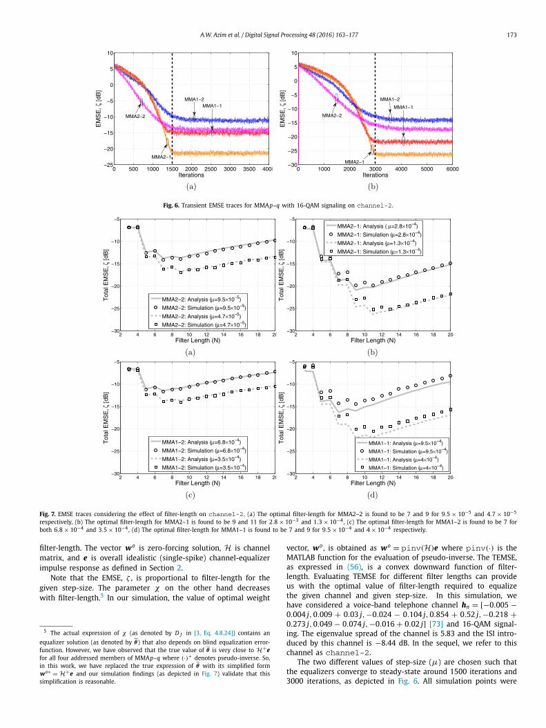
Fig. 6. Transient EMSE traces for MMAp–q with 16-QAM signaling on channel-2.

Fig. 7. EMSE traces considering the effect of filter-length on channel-2. (a) The optimal filter-length for MMA2–2 is found to be 7 and 9 for 9.5 × 10−5 and 4.7 × 10−5

respectively, (b) The optimal filter-length for MMA2–1 is found to be 9 and 11 for 2.8 × 10−3 and 1.3 × 10−4, (c) The optimal filter-length for MMA1–2 is found to be 7 for both 6.8 × 10−4 and 3.5 × 10−4, (d) The optimal filter-length for MMA1–1 is found to be 7 and 9 for 9.5 × 10−4 and 4 × 10−4 respectively.

filter-length. The vector wo is zero-forcing solution, H is channel matrix, and e is overall idealistic (single-spike) channel-equalizer impulse response as defined in Section 2.

Note that the EMSE, ζ , is proportional to filter-length for the given step-size. The parameter χ on the other hand decreases with filter-length.5 In our simulation, the value of optimal weight

5 The actual expression of χ (as denoted by D f in [3, Eq. 4.8.24]) contains an equalizer solution (as denoted by θ ) that also depends on blind equalization error-function. However, we have observed that the true value of θ is very close to H+efor all four addressed members of MMAp–q where (·)+ denotes pseudo-inverse. So, in this work, we have replaced the true expression of θ with its simplified form wo∗ = H+e and our simulation findings (as depicted in Fig. 7) validate that this simplification is reasonable.

vector, wo , is obtained as wo = pinv(H)e where pinv(·) is the MATLAB function for the evaluation of pseudo-inverse. The TEMSE, as expressed in (56), is a convex downward function of filter-length. Evaluating TEMSE for different filter lengths can provide us with the optimal value of filter-length required to equalize the given channel and given step-size. In this simulation, we have considered a voice-band telephone channel hn = [−0.005 −0.004 j, 0.009 + 0.03 j, −0.024 − 0.104 j, 0.854 + 0.52 j, −0.218 +0.273 j, 0.049 − 0.074 j, −0.016 + 0.02 j] [73] and 16-QAM signal-ing. The eigenvalue spread of the channel is 5.83 and the ISI intro-duced by this channel is −8.44 dB. In the sequel, we refer to this channel as channel-2.

The two different values of step-size (μ) are chosen such that the equalizers converge to steady-state around 1500 iterations and 3000 iterations, as depicted in Fig. 6. All simulation points were

174 A.W. Azim et al. / Digital Signal Processing 48 (2016) 163–177

obtained by executing the program 10 times (or runs) with random and independent generation of transmitted data. Each run was exe-cuted for as many iterations as required for the convergence. Once convergence is acquired, the equalizer is run for further 5000 iter-ations for the computation of steady-state value of EMSE. In Fig. 7, we depict analytical and simulated TEMSE obtained as a func-tion of filter-length for the given step-sizes for MMA2–2, MMA2–1, MMA1–2 and MMA1–1. Both analytical and simulated TEMSE are found to be in close agreement.

7.4. Experiment IV: Adaptive polarization demultiplexing

In this experiment we consider an adaptive optical demultiplex-ing scenario. A key part of the digital signal processing receiver unit is to demultiplex the received signal to recover the two or-thogonal polarization tributaries sent from the transmitter end. This can be done using blind adaptive FIR filters, updated using the stochastic gradient algorithm (employing only the demultiplexed sequence) as proposed in [28]. The filters are arranged in a butter-fly structure [74] as shown in Fig. 8 and are continuously updated. Note that the multiplexing phenomenon can be modeled as a Jones matrix. Given the azimuth rotation angle 2θ and the elevation rota-tion angle φ, the unitary 2 × 2 (Jones) matrix R, which represents the baseband model of two multiplexed optical channels, is given by [29]

Fig. 8. Optical butterfly equalizer.

R(θ,φ) =[

cos(θ) sin(θ)exp(− jφ)

−exp( jφ) sin(θ) cos(θ)

]. (57)

Note that the two rows represent multiplexed channels which ro-tate the horizontal and vertical states of polarized transmitted data and convert them into a new but arbitrary pair of orthogonal states. Suppose xn and yn are the transmitted polarization division multiplexed QAM (PDM-QAM) signals, using the channel model, the received polarized signals (which become input to the demul-tiplexer) are[

xinn

yinn

]= R

[xn

yn

](58)

It has to be noted that the two input signals of the block, xinn and

yinn , are a mixture of the two signals emitted along the two or-

thogonal states of polarization of light. Therefore the task of the adaptive equalizer is to estimate the inverse of the Jones matrix so as to reverse the effects induced by the channel propagation. The adaptive equalizer (demultiplexer) wn is an adaptive 2 × 2 matrix and is defined as wn = [wxx

n wxyn ; w yx

n w yyn]. The demultiplexed

signals, xoutn and yout

n , are given by[xout

nyout

n

]= w∗

n

[xin

n

yinn

]=[

(wxxn )∗xin

n + (wxyn )∗ yin

n

(w yxn )∗xin

n + (w yyn )∗ yin

n

](59)

Upon successful convergence of wn , xoutn and yout

n are required to provide estimates of xn and yn , respectively. Due to permutation ambiguity (also known as channel swapping), however, it is pos-sible that xout

n and youtn , instead, provide estimates of yn and xn ,

respectively.6

Since the Jones matrix is considered to be stationary, we have σq = 0 for the analytical evaluation of EMSE. Refer to Fig. 9(a) for

6 For some values of θ and φ , we have found that some members of MMAp–qhappen to recover the signals with poor output signal-to-noise ratio. However, dis-cussing those cases and their remedies are beyond the scope of this work and will be discussed else where.

Fig. 9. (a) EMSE traces for four members of MMAp–q with 16-QAM signaling for R(45◦, 60◦). (b) Scatter plots before and after demultiplexing using MMA2–2 equalizer with μ = 1 × 10−4 (subplots for other equalizers are not shown due to space limitation).

A.W. Azim et al. / Digital Signal Processing 48 (2016) 163–177 175

the comparison of theoretical and simulated EMSE of MMA2–2, MMA2–1, MMA1–2 and MMA1–1 equalizers for R(45◦, 60◦). The legend ‘Closed-form’ refers to the solutions (T2.1), (T3.1), (T4.1) and (T5.1) and the legend ‘Numerical’ refers to (21), (28), (36) and (44)for MMA2–2, MMA2–1, MMA1–2 and MMA1–1 equalizers, respec-tively. As evident from (59), we use N = 2 for the evaluation of analytical EMSE. Also refer to Fig. 9(b) for the scatter plots for re-ceived (multiplexed) and equalized (demultiplexed) signals.

8. Conclusions

This paper reports the steady-state EMSE analysis of adap-tive filters belonging to MMAp–q family (i.e., MMA2–2, MMA2–1, MMA1–2 and MMA1–1) by exploiting the fundamental energy re-lation in non-stationary environment. This relation is fundamental in that it is exact, and it holds without requiring any approxima-tion. Exploiting this relation, we have obtained analytical (closed-form) expressions for EMSE for MMA2–2, MMA2–1, MMA1–2 and MMA1–1 equalizers are verified by computer simulations. From this study, we conclude the following:

1. By using fundamental variance relation, steady-state EMSE analysis for different MMAp–q equalizers can be performed in a simpler way. In particular, we have obtained exact as well as approximate (but closed-form) EMSE expressions for MMA2–2, MMA2–1, MMA1–2 and MMA1–1 equalizers using the fundamental variance relation in a straightforward manner. Our analytical findings have been validated for both station-ary and non-stationary channel environments. Among the four addressed members of MMAp–q, we have also noticed that MMA2–1 is providing the least EMSE in multi-path channel environment.

2. The so-called total EMSE expression has been found useful in determining the optimum lengths of the addressed equal-izers for underlying channels and given values of step-sizes. Our experiments have indicated that the optimum lengths for MMA2–2, MMA2–1, MMA1–2 and MMA1–1 equalizers for a typical (7-tap) voice-band channel are between 7 and 13 de-pendent upon the step-size.

3. There has been a growing trend of application of different variants of MMA and CMA in optical systems for polarization demultiplexing supported with coherent detection. We have evaluated the performance of MMAp–q algorithms in terms of EMSE for the task of adaptive polarization demultiplexing in coherent optical systems.

Acknowledgments

The authors acknowledge the support of COMSATS Institute of Information Technology (Islamabad and Wah Campuses), Pak-istan, the Deanship of Scientific Research at King Fahd University of Petroleum and Minerals under research grant RG1414, Saudi Arabia, and Brunel University London, UK towards the accomplish-ment of this work. They also acknowledge the Editor and anony-mous reviewers for their support and valuable feedback.

Appendix A. Supplementary material

Supplementary material related to this article can be found on-line at http://dx.doi.org/10.1016/j.dsp.2015.09.002.

References

[1] S. Haykin, Blind Deconvolution, PTR Prentice Hall, Englewood Cliffs, 1994.[2] R. Johnson Jr., P. Schniter, T.J. Endres, J.D. Behm, D.R. Brown, R.A. Casas, Blind

equalization using the constant modulus criterion: a review, Proc. IEEE 86 (10) (1998) 1927–1950.

[3] Z. Ding, Y. Li, Blind Equalization and Identification, Marcel Dekker, Inc., New York, Basel, 2001.

[4] B. Friedlander, Lattice filters for adaptive processing, IEEE Proc. 70 (8) (1982) 829–867.

[5] S.J. Orfanidis, Optimum Signal Processing: An Introduction, Macmillan, New York, 1985.

[6] B. Widrow, J.R. Glover Jr., J.M. McCool, J. Kaunitz, C.S. Williams, R.H. Hearn, J.R. Zeidler, E. Dong Jr., R.C. Goodlin, Adaptive noise cancelling: principles and applications, IEEE Proc. 63 (12) (1975) 1692–1716.

[7] S.L. Marple Jr., Digital Spectral Analysis with Applications, vol. 1, Prentice-Hall, Inc., Englewood Cliffs, NJ, 1987.

[8] B. Widrow, S.D. Stearns, Adaptive Signal Processing, vol. 1, Prentice-Hall, Inc., Englewood Cliffs, NJ, 1985.

[9] C.F.N. Cowan, P.M. Grant, P.F. Adams, Adaptive Filters, vol. 152, Prentice-Hall, Englewood Cliffs, 1985.

[10] S. Haykin, Introduction to Adaptive Filters, vol. 984, Macmillan, New York, 1984.

[11] M.L. Honig, D.G. Messerschmitt, Adaptive Filters: Structures, Algorithms, and Applications, Kluwer, 1984.

[12] S.T. Alexander, Adaptive Signal Processing: Theory and Applications, Springer-Verlag, New York, 1986.

[13] B. Widrow, J.M. McCool, M. Larimore, C.R. Johnson Jr., Stationary and nonsta-tionary learning characteristics of the LMS adaptive filter, IEEE Proc. 64 (8) (1976) 1151–1162.

[14] A.H. Sayed, Fundamentals of Adaptive Filtering, John Wiley & Sons, Hoboken, New Jersey, 2003.

[15] D. Godard, Self-recovering equalization and carrier tracking in two-dimensional data communication systems, IEEE Trans. Commun. 28 (11) (1980) 1867–1875.

[16] J. Treichler, M. Larimore, New processing techniques based on the constant modulus adaptive algorithm, IEEE Trans. Acoust. Speech Signal Process. 33 (2) (1985) 420–431.

[17] S. Abrar, A. Zerguine, A.K. Nandi, Adaptive blind channel equalization, in: C. Palanisamy (Ed.), Digital Communication, InTech Publishers, Rijeka, Croatia, 2012, Chapter 6.

[18] A. Benveniste, M. Goursat, Blind equalizers, IEEE Trans. Commun. 32 (8) (1984) 871–883.

[19] K. Wesolowski, Self-recovering adaptive equalization algorithms for digital ra-dio and voiceband data modems, in: Proc. European Conf. Circuit Theory and Design, 1987, pp. 19–24.

[20] K.N. Oh, Y.O. Chin, Modified constant modulus algorithm: blind equaliza-tion and carrier phase recovery algorithm, in: Proc. IEEE Globcom, 1995, pp. 498–502.

[21] G.-H. Im, C.-J. Park, H.-C. Won, A blind equalization with the sign algorithm for broadband access, IEEE Commun. Lett. 5 (2) (2001) 70–72.

[22] S. Abrar, A.K. Nandi, Blind equalization of square-QAM signals: a multimodulus approach, IEEE Trans. Commun. 58 (6) (2010) 1674–1685.

[23] K. Wesolowski, Analysis and properties of the modified constant modulus al-gorithm for blind equalization, Eur. Trans. Telecommun. 3 (3) (1992) 225–230.

[24] J. Yang, J.-J. Werner, G.A. Dumont, The multimodulus blind equalization and its generalized algorithms, IEEE J. Sel. Areas Commun. 20 (5) (2002) 997–1015.

[25] J.-T. Yuan, K.-D. Tsai, Analysis of the multimodulus blind equalization algo-rithm in QAM communication systems, IEEE Trans. Commun. 53 (9) (2005) 1427–1431.

[26] X.-L. Li, W.-J. Zeng, Performance analysis and adaptive Newton algorithms of multimodulus blind equalization criterion, Signal Process. 89 (11) (2009) 2263–2273.

[27] J.-T. Yuan, T.-C. Lin, Equalization and carrier phase recovery of CMA and MMA in blind adaptive receivers, IEEE Trans. Signal Process. 58 (6) (2010) 3206–3217.

[28] K. Kikuchi, Polarization-demultiplexing algorithm in the digital coherent re-ceiver, in: Proc. Digest 2008 IEEE/LEOS Summer Topical Meetings, 2008, pp. 101–102.

[29] S.J. Savory, Digital coherent optical receivers: algorithms and subsystems, IEEE J. Sel. Top. Quantum Electron. 16 (5) (2010) 1164–1179.

[30] E.M. Ip, J.M. Kahn, Fiber impairment compensation using coherent detection and digital signal processing, J. Lightwave Technol. 28 (4) (2010) 502–519.

[31] J. Renaudier, O. Bertran-Pardo, G. Charlet, M. Salsi, H. Mardoyan, P. Tran, S. Bigo, 8 Tb/s long haul transmission over low dispersion fibers using 100 Gb/s PDM-QPSK channels paired with coherent detection, Bell Labs Tech. J. 14 (4) (2010) 27–45.

[32] P. Johannisson, M. Sjödin, M. Karlsson, H. Wymeersch, E. Agrell, P.A. Andrekson, Modified constant modulus algorithm for polarization-switched QPSK, Opt. Ex-press 19 (8) (2011) 7734–7741.

[33] D.S. Millar, S.J. Savory, Blind adaptive equalization of polarization-switched QPSK modulation, Opt. Express 19 (9) (2011) 8533–8538.

[34] I. Roudas, A. Vgenis, C.S. Petrou, D. Toumpakaris, J. Hurley, M. Sauer, J. Downie, Y. Mauro, S. Raghavan, Optimal polarization demultiplexing for coherent optical communications systems, J. Lightwave Technol. 28 (7) (2010) 1121–1134.

[35] A. Vgenis, C.S. Petrou, C.B. Papadias, I. Roudas, L. Raptis, Nonsingular constant modulus equalizer for PDM-QPSK coherent optical receivers, IEEE Photonics Technol. Lett. 22 (1) (2010) 45–47.

176 A.W. Azim et al. / Digital Signal Processing 48 (2016) 163–177

[36] I. Fatadin, D. Ives, S.J. Savory, Blind equalization and carrier phase recovery in a 16-QAM optical coherent system, J. Lightwave Technol. 27 (15) (2009) 3042–3049.

[37] P. Johannisson, H. Wymeersch, M. Sjödin, A.S. Tan, E. Agrell, P.A. Andrekson, M. Karlsson, Convergence comparison of the CMA and ICA for blind polarization demultiplexing, J. Opt. Commun. Netw. 3 (6) (2011) 493–501.

[38] C. Yuxin, H. Guijun, Y. Li, Z. Ling, L. Li, Mode demultiplexing based on multi-modulus blind equalization algorithm, Opt. Commun. 324 (2014) 311–317.

[39] Z. Qu, S. Fu, M. Zhang, M. Tang, P. Shum, D. Liu, Analytical investigation on self-homodyne coherent system based on few-mode fiber, IEEE Photonics Technol. Lett. 26 (1) (2014) 74–77.

[40] J. Zhang, B. Huang, X. Li, Improved quadrature duobinary system performance using multi-modulus equalization, IEEE Photonics Technol. Lett. 25 (16) (2013) 1630–1633.

[41] J. Zhang, J. Yu, N. Chi, Z. Dong, J. Yu, X. Li, L. Tao, Y. Shao, Multi-modulus blind equalizations for coherent quadrature duobinary spectrum shaped pm-qpsk digital signal processing, J. Lightwave Technol. 31 (7) (2013) 1073–1078.

[42] Z. Yu, X. Yi, J. Zhang, M. Deng, H. Zhang, K. Qiu, Modified constant modulus algorithm with polarization demultiplexing in Stokes space in optical coherent receiver, J. Lightwave Technol. 31 (19) (2013) 3203–3209.

[43] X. Zhou, J. Yu, M.F. Huang, Y. Shao, T. Wang, P. Magill, M. Cvijetic, L. Nelson, M. Birk, G. Zhang, S. Ten, H.B. Matthew, S.K. Mishra, Transmission of 32-Tb/s capacity over 580 km using RZ-shaped PDM-8QAM modulation format and cas-caded multimodulus blind equalization algorithm, J. Lightwave Technol. 28 (4) (2010) 456–465.

[44] S. Abrar, A.K. Nandi, Adaptive solution for blind equalization and carrier-phase recovery of square-QAM, IEEE Signal Process. Lett. 17 (9) (2010) 791–794.

[45] S. Abrar, A. Zerguine, A.K. Nandi, Blind adaptive polarization demultiplexing in coherent PDM QAM systems, in: Proc. IEEE FIT, 2014.

[46] I. Fijalkow, C.E. Manlove, R. Johnson Jr., Adaptive fractionally spaced blind CMA equalization: excess MSE, IEEE Trans. Signal Process. 46 (1) (1998) 227–231.

[47] J.J. Shynk, R.P. Gooch, G. Krishnamurthy, C.K. Chan, Comparative performance study of several blind equalization algorithms, Proc. SPIE Conf. Adv. Signal Pro-cess. 1565 (2) (1991) 102–117.

[48] J. Mai, A.H. Sayed, A feedback approach to the steady-state performance of fractionally spaced blind adaptive equalizers, IEEE Trans. Signal Process. 48 (1) (2000) 80–91.

[49] N.R. Yousef, A.H. Sayed, A unified approach to the steady-state and tracking analyses of adaptive filters, IEEE Trans. Signal Process. 49 (2) (2001) 314–324.

[50] S. Abrar, A. Ali, A. Zerguine, A.K. Nandi, Tracking performance of two constant modulus equalizers, IEEE Commun. Lett. 17 (5) (2013) 830–833.

[51] S. Abrar, A.K. Nandi, Adaptive minimum entropy equalization algorithm, IEEE Commun. Lett. 14 (10) (2010) 966–968.

[52] A.W. Azim, S. Abrar, A. Zerguine, A.K. Nandi, Steady-state performance of mul-timodulus blind equalizers, Signal Process. 108 (2015) 509–520.

[53] N. Xie, H. Hu, H. Wang, A new hybrid blind equalization algorithm with steady-state performance analysis, Digit. Signal Process. 22 (2) (2012) 233–237.

[54] T. Thaiupathump, L. He, S.A. Kassam, Square contour algorithm for blind equal-ization of QAM signals, Signal Process. 86 (11) (2006) 3357–3370.

[55] S.A. Sheikh, P. Fan, New blind equalization techniques based on improved square contour algorithm, Digit. Signal Process. 18 (5) (2008) 680–693.

[56] S.A. Sheikh, P. Fan, Two efficient adaptively varying modulus blind equalizers: AVMA and DM/AVMA, Digit. Signal Process. 16 (6) (2006) 832–845.

[57] M.G. Larimore, J.R. Treichler, Convergence behavior of the constant modulus algorithm, in: Proc. IEEE ICASSP, vol. 8, 1983, pp. 13–16.

[58] V. Weerackody, S.A. Kassam, K.R. Laker, Sign algorithms for blind equaliza-tion and their convergence analysis, Circuits Syst. Signal Process. 10 (4) (1991) 393–431.

[59] T.Y. Al-Naffouri, A.H. Sayed, Adaptive filters with error nonlinearities: mean-square analysis and optimum design, EURASIP J. Appl. Signal Process. 1 (2001) 192–205.

[60] D. Dohono, On minimum entropy deconvolution, in: Proc. 2nd Applied Time Series Symp., 1980, pp. 565–608.

[61] M.T.M. Silva, M.D. Miranda, Tracking issues of some blind equalization algo-rithms, IEEE Signal Process. Lett. 11 (9) (2004) 760–763.

[62] N. Xie, H. Hu, H. Wang, A new hybrid blind equalization algorithm with steady-state performance analysis, Digit. Signal Process. 22 (2) (2012) 233–237.

[63] J. Mendes Filho, M.D. Miranda, M. Silva, A regional multimodulus algorithm for blind equalization of QAM signals: introduction and steady-state analysis, Signal Process. 92 (11) (2012) 2643–2656.

[64] M. Niroomand, M. Derakhtian, M.A. Masnadi-Shirazi, Steady-state performance analysis of a generalised multimodulus adaptive blind equalisation based on the pseudo Newton algorithm, IET Signal Process. 6 (1) (2012) 14–26.

[65] B. Lin, R. He, X. Wang, B. Wang, The excess mean-square error analyses for Bussgang algorithm, IEEE Signal Process. Lett. 15 (2008) 793–796.

[66] A. Goupil, J. Palicot, A geometrical derivation of the excess mean square er-ror for Bussgang algorithms in a noiseless environment, Signal Process. 84 (2) (2004) 311–315.

[67] N. Gu, W. Yu, D. Creighton, S. Nahavandi, Selecting optimal norm and step size of generalised constant modulus algorithms under non-stationary envi-ronments, Electron. Lett. 46 (25) (2010) 1673–1674.

[68] S. Bellini, Bussgang techniques for blind deconvolution and equalization, in: Blind Deconvolution, Prentice Hall, Upper Saddle River, N.J., 1994.

[69] T.Y. Al-Naffouri, A.H. Sayed, Transient analysis of adaptive filters with error nonlinearities, IEEE Trans. Signal Process. 51 (3) (2003) 653–663.

[70] O. Dabeer, E. Masry, Convergence analysis of the constant modulus algorithm, IEEE Trans. Inf. Theory 49 (6) (2003) 1447–1464.

[71] P. Bello, Characterization of randomly time-variant linear channels, IEEE Trans. Commun. Syst. 11 (4) (1963) 360–393.

[72] C. Komninakis, C. Fragouli, A.H. Sayed, R.D. Wesel, Multi-input multi-output fading channel tracking and equalization using Kalman estimation, IEEE Trans. Signal Process. 50 (5) (2002) 1065–1076.

[73] G. Picchi, G. Prati, Blind equalization and carrier recovery using a “stop-and-go” decision-directed algorithm, IEEE Trans. Commun. 35 (9) (1987) 877–887.

[74] R. Raheli, G. Picchi, Synchronous and fractionally-spaced blind equalization in dually-polarized digital radio links, in: IEEE ICC, 1991, pp. 156–161.

Ali Waqar Azim received his Bachelor of Science in Electrical (Telecommunication) Engineering with distinction from COMSATS Institute of Information Technology, Islamabad, Pakistan. He obtained Diplôme d’ingénieur (Engineering Diploma) in Telecommuni-cation Engineering and Laurea Magistrale in Ingeg-neria Elettronica (Masters in Electronic Engineering) from ENSIMAG, Institut Polytechnique de Grenoble, France, and Politechnico di Torino, Italy, respectively.

Presently, he is working as a Lecturer at COMSATS Institute of Information Technology, Wah, Pakistan. His research interest is in Signal Processing and Digital Communications.

Shafayat Abrar was born in Karachi, Pakistan, in 1972. He holds a B.E. degree in electrical engineer-ing from NED University of Engineering and Tech-nology, Karachi, Pakistan (I996) and an M.S. degree in electrical engineering from King Fahd University of Petroleum and Minerals (KFUPM), Dhahran, Saudi Arabia (2000). He earned his Ph.D. degree in electri-cal engineering from The University of Liverpool, Liv-erpool, UK (2010). He has been co-recipient of Best

Paper Award of IEEE-INCC’04 at Lahore University of Management Sciences, Lahore, Pakistan. He has been co-recipient of IEEE Communications Soci-ety Heinrich Hertz Award for Best Communications Letters at IEEE GLOBECOM 2012 event in Anaheim, CA, USA.

Professor Azzedine Zerguine received the B.Sc. degree from Case Western Reserve University, Cleve-land, OH, USA, in 1981, the M.Sc. degree from King Fahd University of Petroleum and Minerals (KFUPM), Dhahran, Saudi Arabia, in 1990, and the Ph.D. degree from Loughborough University, Loughborough, UK, in 1996, all in electrical engineering. He is currently a Professor in the Electrical Engineering Department, KFUPM, working in the areas of signal processing and

communications. Dr. Zerguine was the recipient of three Best Teaching Awards, in 2000, 2005, and 2011 at KFUPM. He is presently serving as an Associate Editor of the EURASIP Journal on Advances in Signal Process-ing.

Professor Asoke K. Nandi received the degree of Ph.D. from the University of Cambridge (Trinity Col-lege), Cambridge (UK). He held academic positions in several universities, including Oxford (UK), Imperial College London (UK), Strathclyde (UK), and Liverpool (UK). In 2013 he moved to Brunel University (UK), to become the Chair and Head of Electronic and Com-puter Engineering. Professor Nandi is a Distinguished Visiting Professor at Tongji University (China), and an

Adjunct Professor at University of Calgary (Canada).

A.W. Azim et al. / Digital Signal Processing 48 (2016) 163–177 177

His current research interests lie in the areas of signal processing and machine learning, with applications to communications, gene expres-sion data, functional magnetic resonance data, and biomedical data. He has made many fundamental theoretical and algorithmic contributions to many aspects of signal processing and machine learning. He has much expertise in “Big Data”, dealing with heterogeneous data, and extractinginformation from multiple datasets obtained in different laboratories and different times. He has authored over 500 technical publications, including 200 journal papers as well as four books.

Professor Nandi is a Fellow of the Royal Academy of Engineering and also a Fellow of seven other institutions including the IEEE and the IET. Among the many awards he received are the Institute of Electrical and Electronics Engineers (USA) Heinrich Hertz Award in 2012, the Glory of Bengal Award for his outstanding achievements in scientific research in 2010, the Water Arbitration Prize of the Institution of Mechanical Engi-neers (UK) in 1999, and the Mountbatten Premium, Division Award of the Electronics and Communications Division, of the Institution of Electrical Engineers (UK) in 1998.