Embed Size (px)
Citation preview
DIGITAL WATERMARKING
BASED ON HUMAN VISUAL SYSTEM
A THESIS SUBMITTED TO
THE GRADUATE SCHOOL OF NATURAL AND APPLIED SCIENCES
OF
THE MIDDLE EAST TECHNICAL UNIVERSITY
BY
ALPER KOZ
IN PARTIAL FULFILLMENT OF THE REQUIREMENTS FOR THE DEGREE OF
MASTER OF SCIENCE
IN
THE DEPARTMENT OF ELECTRICAL AND ELECTRONICS ENGINEERING
SEPTEMBER 2002

Approval of the Graduate School of Natural and Applied Sciences
Prof. Dr. Tayfur Öztürk Director
I certify that this thesis satisfies all the requirements as a thesis for the degree
of Master of Science.
Prof. Dr. Mübeccel Demirekler Head of Department
This is to certify that we have read this thesis and that in our opinion it is fully
adequate, in scope and quality, as a thesis for the degree of Master of Science.
Assoc. Prof. Dr. A. Aydın Alatan Supervisor
Examining Committee Members
Prof. Dr. Levent Onural
Assoc. Prof. Dr. A. Aydın Alatan
Assoc. Prof. Dr. Gözde Bozdağı Akar
Assoc. Prof. Dr. Tolga Çiloğlu
Assoc. Prof. Dr. Engin Tuncer

�
� iii�
ABSTRACT�
��
DIGITAL�WATERMARKING�BASED�ON�HUMAN�VISUAL�SYSTEM�
�
�
�
Koz,�Alper�
�
�
M.Sc.,�Department�of�Electrical�and�Electronics�Engineering�
�
�
Supervisor:�Assoc.�Prof.�Dr.�A.�Aydın�Alatan�
��
September�2002,�80�pages�
��
The�recent�progress�in�the�digital�multimedia�technologies�has�offered�many�facilities�
in� the�transmission,� reproduction�and�manipulation�of�data.� �However,� this�advance�
has� also� brought� the� problem� such� as� copyright� protection� for� content� providers.�
Digital� watermarking� is� one� of� the� proposed� solutions� for� copyright� protection� of�
multimedia.� A� watermark� embeds� an� imperceptible� signal� into� data� such� as� audio,�
image�and�video,�which�indicates�whether�or�not�the�content� is�copyrighted.�Within�
this� scope,� digital� watermarking� methods,� which� are� designed� to� exploit� many�
aspects� of� HVS� in� order� to� provide� an� imperceptible� and� robust� watermark,� are�
reviewed.� Then,� two� watermarking� methods,� which� are� based� on� foveation� and�

�
� iv�
temporal sensitivity� phenomena� of� HVS,� respectively,� are� proposed.� These�
approaches�have�not�been�exploited�for�the�purpose�of�digital�watermarking.�The�first�
proposed� method� embeds� watermark� into� the� image� periphery� according� to�
foveation-based� HVS� contrast� thresholds.� Compared� to� the� other� HVS-based�
watermarking� methods,� the� simulation� results� demonstrate� an� improvement� in� the�
robustness� of� the� proposed� approach� against� image� degradations,� such� as� JPEG�
compression,� cropping� and� additive� Gaussian� noise.� In� addition,� the� proposed�
method�for�the�images�is�adapted�for�video�and�the�robustness�of�the�adapted�method�
against�ITU�H263+�coding�is�tested.�The�second�method,�which�is�proposed�for�only�
video�watermarking,�exploits� the� temporal�contrast� thresholds�of�HVS�to�determine�
the�location,�where�the�watermark�should�be�embedded�and�the�maximum�strength�of�
the� watermark.� The� results� demonstrate� that� the� proposed� scheme� survives� video�
distortions,�such�as�additive�Gaussian�noise,�ITU�H263+�coding�at�bit�rates�not�lower�
than�230-240�kbps,�frame�dropping�and�frame�averaging.����
�
Keywords:� Digital� Watermarking,� Human� Visual� System,� Contrast� thresholds,�
Contrast�Masking,�Foveation,�Temporal�Sensitivity,�H.263.���
�
�
���
����������

�
� v
ÖZ�
�
�
İNSAN�GÖRME�SİSTEMİNE�DAYALI �GÖRÜNMEZ�
DAMGALAMA�
�
�
Koz,�Alper�
�
�
Yüksek�Lisans,�Elektrik�ve�Elektronik�Mühendisliği�Bölümü�
Tez�yöneticisi:�Doç.�Dr.�A.�Aydın�Alatan�
�
�
Eylül�2002,�80�sayfa�
�
�
Son�yıllarda�sayısal�teknolojinin�gelişimi�sayısal�bilginin�üretilmesinde,�iletilmesinde�
ve�kullanımında�büyük�kolaylıklar�sağlamıştır.��Fakat,�bu�gelişme�aynı�zamanda�telif�
hakkının� korunması� gibi� bir� problemi� daha� da� belirgin� hale� getirmiştir.� Görünmez�
sayısal�damgalama�bu�soruna�önerilen�çözümlerden�birisidir.�Görünmez�damga�ses,�
imge�ve�video�gibi�bilgilerin� içine�saklanır�ve�bilginin� izinsiz�kullanımı�durumunda�
telif� hakkı� sahibinin� kendi� sahipliğini� ispatlamasını� sağlar.� Bu� çerçevede,� insan�
görme� sisteminin� (İGS)� özelliklerini� kullanan� görünmez� damgalama� yöntemleri�
incelenmiş� ve� İGS’nin� odaklanma� özelliğine� ve� zamansal� değişimlere�duyarlılığına�
dayalı� iki� farklı� yöntem� önerilmiştir.� Birinci� yöntem,� odaklanmaya� dayalı� kontrast�
eşik�değerlerini�kullanarak,��odaklanılan��noktadan�uzaklaştıkça�damganın�büyüklüğü��

�
� vi�
artacak� şekilde�damgayı� imgeye�koyar.�Yöntemin� toplamsal�Gauss�gürültüsü,� imge�
kırpma�ve�imge�sıkıştırma�(JPEG)�gibi�ataklara�dayanıklılığı�ve�daha�önceki�İGS’ye�
dayalı� yöntemlerden� daha� iyi� sonuçlar� verdiği� gösterilmiştir.� Ayrıca� yöntem� video�
için� uyarlanmış� ve� yöntemin� ITU� H263+� kodlamasına� karşı� gürbüzlüğü�
gösterilmiştir.� Sadece� video� damgalama� için� önerilen� ikinci� yöntem� ise,� İGS’nin�
zamansal� kontrast� eşik� düzeylerinden� faydalanarak� damganın� videonun� hangi�
kısımlarına� konacağını� ve� damganın� büyüklüğünü� belirler.� Yöntemin,� ITU� H263+�
kodlama� (230-240� kbps’den� daha� büyük� bit� hızları� için),� Gauss� gürültüsü� ekleme,�
çerçevelerin� ortalamasını� alma� ve� çerçeve�düşürme� gibi� ataklara� karşı� dayanıklılığı�
gösterilmiştir.���
Anahtar� Kelimeler:� � İnsan� Görme� Sistemi,� Görünmez� Damgalama,� Odaklanma,�
H263+,�Zamansal�Kontrast�Eşik�Düzeyi.��
�
�
�
�
�
�
�
�
�
�
�
�
�
�
�
�
�

�
�vii�
�
�
�
ACKNOWLEDGMENTS��
I� would� like� to� thank� my� supervisor,� Assoc.� Prof.� A� Aydın� Alatan� for� his� valuable�
supervision�and�support�during�the�preparation�of�this�thesis.��
�
�
�
�
�
�
�
�
�
�
�
�
�
�
�
�
�
�
�
�
�
�
�
�

�
�viii�
�
�
�
TABLE�OF�CONTENTS�
�
ABSTRACT�� iii��
ÖZ�� v�
ACKNOWLEDGEMENTS�� vii�
TABLE�OF�CONTENTS�������������������������������������������������������������������������������������������������������viii��
LIST�OF�TABLES�� x�
LIST�OF�FIGURES� xi�
LIST�OF�ABBREVIATIONS������������������������������������������������������������������������������������������������xiii�
�
CHAPTER�
1� INTRODUCTION�� 1�
1.1�Watermarking�Applications� 2��
1.2�Watermarking�Requirements��� 3��
1.3�Trade�off�between�requirements� 5��
1.4�The�importance�of�vision�models�� 7�
1.5� Problem�Statement�� 9�
1.6� Outline�of�Dissertation�� 9�
2� BASICS�OF�HUMAN�VISUAL�SYSTEM� 11��
� 2.1�Contrast�and�Contrast�thresholds� 11�
2.1.1�Light�Adaptation� 14��
2.1.2�Contrast�Masking� 17�
� 2.2�Spatial�and�Temporal�Masking�� 23��
2.3� Foveation�� 26�
2.4� Temporal�Sensitivity� 33�
� � 2.4.1�Fundamental�Definitions� 34��
2.4.2�Temporal�Contrast�Sensitivity�Function�� 35�

�
� ix�
2.4.3�Temporal�Contrast�Thresholds�For�spatial�DCT�frequencies� 39�
� 3� WATERMARKING�BASED�ON�VISUAL�MODELS� 41��
3.1�Image�Watermarking�Methods�based�on�Visual�Models��� 41�
3.2�Video�Watermarking�Methods�based�on�Visual�models�� 45�
�
� 4� FOVEATED�IMAGE�WATERMARKING� 47�
4.1�Introduction� 47�
4.2�Foveation� 48��
4.3�Proposed�Watermarking�Method�� 49�
4.4�Adaptation�of�the�Method�to�Videos� 53�
4.5�Experimental�Results�� 53�
� 5�� TEMPORAL�WATERMARKING�OF�DIGITAL�VIDEOS� 59�
5.1�Introduction�� 59�
5.2�Watermarking�Procedure� 61�
5.3�Watermark�Detection�� 63��
5.4�Simulation�Results�� 65��
� 5.4.1�Robustness�to�Additive�Gaussian�noise.�� 69�
� 5.4.2�Robustness�to�ITU�H263�+�Coding�� 70�
� 5.4.3�Robustness�to�Frame�Averaging�and�Dropping� 71�
� 6� SUMMARY�AND�DISCUSSIONS� 75�
� �
REFERENCES� 77�
�
�
�
�
�
�
�
�
�
�
� x
LIST�OF�TABLES���TABLE�
�
2.1�Quantization�levels�for�four�levels�DWT�transform.� 22�
� 4.1�Correlation�Results�against�Cropping�� 57�
� 4.2�Correlation�Results�against�Additive�Gaussian�Noise� 57�
� 4.3�Correlation�Results�against�JPEG�Compression�� 57�
�� 4.4�Correlation�Results�against�ITU�H263+�Coding� 58�
� 5.1�Correlation�Results�for�Coast�and�Carphone�Sequences�after��
�� ��Additive�Gaussian�Noise��� 69�
� 5.2�Correlation�Results�for�Coast�and�Carphone�Sequences�after��
� ���ITU�H263+�Coding��� 71�
� 5.3�Correlation�Results�for�Coast�and�Carphone�Sequences�after��
� ��after�frame�dropping���� 72�
� 5.4�Correlation�Results�for�Coast�and�Carphone�Sequences�after��
� ��frame�averaging�� 72�
�
�
�
�
�
�
�
�
�
�

�
� xi�
LIST�OF�FIGURES�
�
FIGURE�
�
� 1.1�� General�Scheme�for�Watermarking�� � � � � � 2�
1.2�����The�illustration�of�the�trade�off�between�the�imperceptibility�and�robustness� 6�
��1.3������An�example�illustrating�perceptual�brightness�is�not�a�monotonic�function�of�
intensity� � � � � � � � � 8�
2.1� Demonstration�of�apparent�brightness�is�not�only�dependent�to��
����������absolute�luminance� � � � � � � � 12�
2.2� Examples�for�the�spatial�patterns�where�the�Weber�contrast�is�used�� � 12�
2.3� The�demonstration�of�Michelson�contrast�for�a�sinusoidal�grating�of�a�spatial�
frequency.��� � � � � � � � � 13�
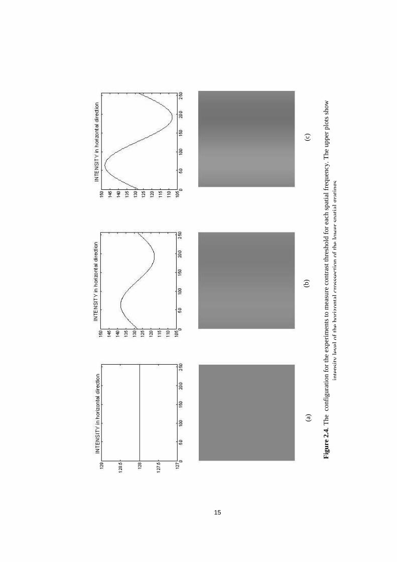
2.4� The��configuration�for�the�experiments�to�measure�contrast�threshold� � 15�
2.5� Contrast�sensitivity�as�a�function�of�spatial�frequency.� � � � 16��
2.6� The�change�in�the�detection�threshold�as�a�function�of�a�mean�luminance.� � 16�
2.7� The��configuration�for�the�experiments�conducted�to�study�contrast�masking.� 20�
2.8� The�amplitude�of�the�signal�in�...�������������� � � � � 21�
2.9� The�demonstration�of�the�change�in�contrast�threshold�as�a�function�of�masker�
contrast. � ������������� � � � � � � 22�
2.10� Visibility�Thresholds�for�a�narrow�bar�of�a�white�noise�in�the�… � ������������� 24�
2.11� Visibility�Thresholds�for�a��40�ms.�flash�of�dynamic�white�…� � � 25��
2.12� �Anatomy�of��human�eye�� � � � � � � 26�
2.13���Rods,�cones�and�ganglion�cells�density�as�a�function�of�eccentricity.��� � 27�
2.14����Original�Lena�Image�and�its�foveated�version�� � � � � 27�
� 2.15����The�configuration�for�the�experiments�to�determine…� � � � 29�
� 2.16����Contrast�Sensitivity�for�patches�of�sinusoidal�grating�as�a�function…� � 29�
2.17����The�configuration�for�the�experiments�to�determine�the�critical�…�� � 31�
2.18����Discrete�wavelet�transform�structure��� � � � � � 32�
2.19����Some�terms�to�describe�visual�stimuli.��� � � � � � 34�

�
�xii�
2.20��The�target�in�(a)�is�modulated�with�respect�to�the�…� � � � 36�
2.21��Temporal�Contrast�Sensitivity�Function�of�HVS.�� � � � � 37�
2.22��The�spatial�configurations�of�the�two�different�targets.�� � � � 38�
2.23��The�effect�of�spatial�frequency�upon�temporal�contrast…� � � � 38�
2.24��Temporal�contrast�thresholds�for�spatial�DCT�frequencies…�� � � 40�
2.25��Temporal�(a),�spatial�(b)�and�orientation�(c)�components�of�…�� � � 40�
4.1����Typical�Geometry.��� � � � � � � � 48�
4.2����Contrast�Threshold�Weight�Function�� � � � � � 50�
4.3����Illustration�of�the�difference�between�the�previous�…� � � � 52�
4.4����Original�image�and�watermarked�image�according�to�proposed�method�� � 55�
4.5����(a)�original�image,�(b)�watermarked�image�according�to�proposed…�� � 56�
5.1����Overall�structure�of�the�watermarking�process.� � � � � 61�
5.2����Overall�structure�of�the�watermark�detection�process.� � � � 64�
5.3����Frame�from�Coast�video.�(a)�original�frame,�(b)�watermarked�frame.�� � 66�
5.4����Frame�from�Carphone �video.�(a)�original�frame,�(b)�watermarked�frame.�� � 66�
5.5����The�number�of�watermarked�coefficients�vs.�discrete�temporal…�� � � 67�
5.6����Illustration�of�where�the�watermark�are�embedded…� � � � 68�
5.7����Mean�of�the�inner�product�results�(see�Eqn.�(5.5))�as�a�function�of�the��
���������discrete�temporal�frequency�after�additive�Gaussian�noise.�� � � � 70�
5.8� ��Mean�of�the�inner�product�results�(see�Eqn.�(5.5))�as�a�function�of�the�discrete�temporal�����
���������frequency�after�ITU�H263+�coding�at�a�bit�rate�of�230�kbps.�� � � 71�
5.9� ��Mean�of�the�inner�product�results�(see�Eqn.�(5.5))�as�a�function�of�the�discrete�temporal��
���������frequency�after�frame�dropping.�� � � � � � � 73�
5.10��Mean�of�the�inner�product�results�(see�Eqn.�(5.5))�as�a�function�of�the�discrete�temporal�
���������frequency�after�frame�averaging.�� � � � � � � 74�
�
�������
�
�xiii�
LIST�OF�ABBREVIATIONS��
�
CIF� � Common�Interface�Format�
CT�� � Contrast�Threshold��
CS� � Contrast�Sensitivity�
DCT� � Discrete�Cosine�Transform�
DWT�� � Discrete�Wavelet�Transform��
HVS� � Human�Visual�System��
IDCT� � Inverse�Discrete�Cosine�Transform�
ITU� � International�Telecommunication�Union�
PSNR� � Peak�Signal�to�Noise�Ratio�
TCSF� � Temporal�Contrast�Sensitivity�Function��
QCIF� � Quarter�Common�Interface�Format�
� �
�
�
�
�
�
�
�
�
�
�
�
�

�
� 1
CHAPTER�1�
���
INTRODUCTION��
�
�
In� recent� years,� digital� multimedia� technology� has� shown� a� significant� progress.� This�
technology� offers� so� many� new� advantages� compared� to� the� old� analog� counterpart.� The�
advantages� during� the� transmission� of� data,� easy� editing� any� part� of� the� digital� content,�
capability� to�copy�a�digital�content�without�any�loss�in�the�quality�of�the�content�and�many�
other� advantages� in� DSP,� VLSI� and� communication� applications� have� made� the� digital�
technology� superior� to� the� analog� systems.� Particularly,� the� growth� of� digital� multimedia�
technology�has�shown� itself�on� Internet�and�wireless�applications.�Yet,� the�distribution�and�
use�of�multimedia�data�is�much�easier�and�faster�with�the�great�success�of�Internet.��
� The� great� explosion� in� this� technology� has� also� brought� some� problems� beside� its�
advantages.� The� great� facility� in� copying� a� digital� content� rapidly,� perfectly� and� without�
limitations�on�the�number�of�copies�has�resulted�the�problem�of�copyright�protection.�Digital�
watermarking�is�proposed�as�a�solution�to�prove�the�ownership�of�digital�data.�A�watermark,�
a�secret�imperceptible�signal,�is�embedded�into�the�original�data�in�such�a�way�that�it�remains�
present�as�long�as�the�perceptible�quality�of�the�content�is�at�an�acceptable�level.�The�owner�
of� the� original� data� proves� his/her� ownership� by� extracting� the� watermark� from� the�
watermarked�content�in�case�of�multiple�ownership�claims.�
� A� general� scheme� for� digital� watermarking� is� given� in� Figure� 1.1.� The� secret�
signature�(watermark)�is�embedded�to�the�cover�image�by�using�a�secret�key�at�the�coder�(C).�
Only�the�owner�of�the�data�knows�the�key�and�it�is�not�possible�to�remove�the�message�from�
the�data�without�the�knowledge�of�the�key.�Then,�the�watermarked�image�passes�through�the�
transmission�channel.�The�transmission�channel� includes�the�possible�attacks,�such�as� lossy�
compression,� geometric� distortions,� any� signal�processing�operation�and�digital-analog�and�
analog�to�digital�conversion,�etc.��After�the�watermarked�image�passes�through�these�possible�
operations,�the�message�is�tried�to�be�extracted�at�the�decoder�(D).��

�
� 2�
�
�
�
Figure�1.1�General�Scheme�for�Watermarking��
�
1.1�Watermarking�Applications��
�
Although�the�main�motivation�behind�the�digital�watermarking�is�the�copyright�protection,�its�
applications�are�not�that�restricted.�There�is�a�wide�application�area�of�digital�watermarking,�
including�broadcast�monitoring,� fingerprinting,�authentication�and�covet�communication� [1,�
2,3,4].��
By�embedding�watermarks� into�commercial�advertisements,� the�advertisements�can�
be�monitored�whether�the�advertisements�are�broadcasted�at�the�correct�instants�by�means�of�
an�automated�system�[1,2].�The�system�receives�the�broadcast�and�searches�these�watermarks�
identifying�where�and�when�the�advertisement�is�broadcasted.��The�same�process�can�also�be�
used�for�video�and�sound�clips.�Musicians�and�actors�may�request�to�ensure�that�they�receive�
accurate�royalties�for�broadcasts�of�their�performances.��
Fingerprinting� is� a� novel� approach� to� trace� the� source� of� illegal� copies� [1,2].� The�
owner� of� the�digital� data�may�embed�different�watermarks� in� the� copies�of�digital� content�
customized� for� each� recipient.� � In� this� manner,� the� owner� can� identify� the� customer� by�
extracting�the�watermark�in�the�case�the�data�is�supplied�to�third�parties.�

�
� 3�
The� digital� watermarking� can� also� be� used� for� authentication� [1,2].� The�
authentication�is�the�detection�of�whether�the�content�of�the�digital�content�has�changed.�As�a�
solution,�a�fragile�watermark�embedded�to�the�digital�content�indicates�whether�the�data�has�
been�altered.�If�any�tampering�has�occurred�in�the�content,� the�same�change�will�also�occur�
on�the�watermark.�It�can�also�provide�information�about�the�part�of�the�content�that�has�been�
altered.��
Covert�communication�is�another�possible�application�of�digital�watermarking�[1,2].�
The�watermark,�secret�message,�can�be�embedded�imperceptibly�to�the�digital�image�or�video�
to�communicate�information�from�the�sender�to�the�intended�receiver�while�maintaining�low�
probability�of�intercept�by�other�unintended�receivers.�
� There� are� also� non-secure� applications� of� digital� watermarking.� It� can� be� used� for�
indexing�of�videos,�movies�and�news�items�where�markers�and�comments�can�be�inserted�by�
search� engines� [2].� Another� non-secure� application� of� watermarking� is� detection� and�
concealment� of� image/video� transmission� errors� [5].� For� block� based� coded� images,� a�
summarizing�data�of�every�block�is�extracted�and�hidden�to�another�block�by�data�hiding.�At�
the�decoder�side,�this�data�is�used�to�detect�and�conceal�the�block�errors.�
�
�1.2�Watermarking�Requirements���
The�efficiency�of�a�digital�watermarking�process�is�evaluated�according�to�the�properties�of�
perceptual�transparency,�robustness,�computational�cost,�bit�rate�of�data�embedding�process,�
false�positive�rate,�recovery�of�data�with�or�without�access�to�the�original�signal,�the�speed�of�
embedding� and� retrieval� process,� the� ability� of� the� embedding� and� retrieval� module� to�
integrate�into�standard�encoding�and�decoding�process�etc.�[1,�2,�6,�7].��
Depending� on� the� application,� the� properties,� which� are� used� mainly� in� the�
evaluation� process,� varies.� For� example,� in� the� video� indexing� application,� evaluating� the�
robustness�of�a�watermarking�scheme�to�any�signal�processing�is�meaningless,�since�there�is�
no� case� that� the� video� passes� through� some� signal� processing� operation.� In� the� covert�
communication�application,�it�is�better�to�use�a�watermarking�scheme�that�does�not�need�the�
original�data�during�the�watermark�detection�process,�if�real�TV�broadcasting�is�used�as�the�
communication�channel,�while�most�of�the�watermarking�schemes�in�other�applications�need�
the�original�data�during�the�detection�process.� If� the�application�is�the�copyright�protection,�
the�owner�of� the�original�data�may�wait� for� several�days� to� insert/detect�watermark,� if� the�
data�is�valuable�for�the�owner.��On�the�other�hand,�in�a�broadcast�monitoring�application,�the�

�
� 4�
speed� of� the� watermark� detection� algorithm� should� be� as� fast� as� the� speed� of� real� time�
broadcasting.�As�a� result,�each�watermarking�application�has� its�own� requirements�and� the�
efficiency�of�the�watermarking�scheme�should�be�evaluated�according�to�these�requirements.��
� As�noted,� the�main�motivation�behind�digital�watermarking� is�copyright�protection.�
The�owner�of�the�original�data�wants�to�prove�his/her�ownership�in�case�the�original�data�is�
copied,� edited� and� used� without� permission� of� the� owner.� In� the� watermarking� research�
world,� this� problem� has� been� analyzed� in� a� more� detailed� manner� [7,� 8,� 9,� 10,� 11,� 12].�
Researchers� on� this� area� focused� on� the� requirements� to� provide� useful� and� effective�
watermarks� for� copyright� protection.� The� requirements� for� an� effective� watermark� are�
imperceptibility,�robustness�to�intended�or�non-intended�any�signal�operations�and�capacity.��
The� imperceptibility� refers� to� the� perceptual� similarity� between� the� original� and�
watermarked� data.� The� owner� of� the� original� data� mostly� does� not� tolerate� any� kind� of�
degradations�in�his/her�original�data.�Therefore,�the�original�and�watermarked�data�should�be�
perceptually� the� same.� The� imperceptibility� of� the� watermark� is� tested� by� means� of� some�
subjective� experiments� [8].� The� original� data� and� watermarked� data� are� presented� to� a�
number�of�subjects,�randomly.�The�subjects�are�asked�the�quality�of�which�work,�original�or�
watermarked�data�is�more�pleasant.�If�the�percentage�of�the�answers�for�each�of�the�two�data�
is� approximately� equal� to� %50,� then� the� watermarked� data� is� perceptually� equal� to� the�
original�data.��
Robustness� to� a� signal� processing� operation� refers� to� the� ability� to� detect� the�
watermark,�after� the�watermarked�data�has�passed�through�that�signal�processing�operation.�
The�robustness�of�a�watermarking�scheme�can�vary�from�one�operation�to�another.�Although�
it�is�possible�for�a�watermarking�scheme�to�be�robust�to�any�signal�compression�operations,�it�
may�not�be�robust�to�geometric�distortions�such�as�cropping,�rotation,�translation�etc.�(for�the�
case,� the�data� is� an� image).� The� signal� processing�operations,� for�which� the�watermarking�
scheme� should� be� robust,� changes� from� application� to� application� as� well.� While,� for� the�
broadcast� monitoring� application,� only� the� robustness� to� the� transmission� of� the� data� in� a�
channel� is� sufficient,� this� is� not� the� case� for� copyright� protection� application� of� digital�
watermarking.� For� such� a� case,� it� is� totally� unknown� through� which� signal� processing�
operations� the� watermarked� data� will� pass.� Hence,� the� watermarking� scheme� should� be�
robust�to�any�possible�signal�processing�operations,�as�long�as�the�quality�of�the�watermarked�
data�preserved.�
The�capacity�requirement�of�the�watermarking�scheme�refers�to�be�able�to�verify�and�
distinguish�between�different�watermarks�with�a� low�probability�of�error�as� the�number�of�

�
� 5�
differently� watermarked� versions� of� an� image� increases� [11].� While� the� robustness� of� the�
watermarking� method� increases,� the� capacity� also� increases� where� the� imperceptibility�
decreases.�There�is�a�trade�off�between�these�requirements�and�this�trade�off�should�be�taken�
into�account�while�the�watermarking�method�is�being�proposed.��
�
1.3�Trade�off�Between�Requirements�
�
In�order� to�show� the� trade�off�between� the� robustness�and� imperceptibility� requirements,�a�
popular�spread�spectrum�image�watermarking�method� is�examined�[7].� In� this�method,� first�
two-dimensional� Discrete� Cosine� Transform� (DCT)� of� the� image� is� computed.� Then,� the�
maximum� 1000� largest� coefficients� are� determined� and� the� watermark� sequence� of� length�
1000,�which�is�generated�from�a�zero�mean�unit�variance�Gaussian�distribution,� is�added�to�
those�coefficients�by�using�the�following�relation:��
�
)),(.1)(,(),( * vuWvuIvuI α+= ���������������������������������������������(1.1)�
�
where� *),( vuI �is�the�watermarked�coefficients,� ),( vuI is�the�DCT�coefficients�of�the�original�
image,� ),( vuW is� the� watermark� component� added� to� the� thvu ),( � DCT� coefficient� of� the�
image�and� α is� the�scale� factor� that�determines� the� trade�off�between� � imperceptibility�and�
robustness.�If� α increases,�obviously�the�added�energy�to�the�image�will�increase�and�it�will�
be�easier�to�detect�the�watermark.�In�other�words,�the�robustness�of�the�watermarking�scheme�
improves�with�a�greater�α .�On�the�other�hand,�an�increase�in�α �produces�more�distortion�in�
the�image.�The�different�watermarked�images�for�different� α values�are�illustrated�in�Figure�
1.2.� As� α increases,� the� distortion� in� the� image� becomes� more� severe.� � Therefore,� the�
maximum�value�of� α ,�which�still�does�not�result�perceptible�distortion�in�the�image,�should�
be�determined� to�achieve�maximum� robustness.� In� [7],� α is� taken�as�0.1.�Such�a� trade�off�
will�always�exist�between�different�requirements.�Hence�the�“best” �method�is�determined�by�
the�application.���
�
�
�

�
� 6�
�� �
(a)���������������������������������������������������������������������(b)�
�
(c)���������������������������������������������������������������������(d)�
�
Figure�1.2�The�illustration�of�the�trade�off�between�the�imperceptibility�and�robustness.�The�
original�image�is�watermarked�by�using�the�Spread�Spectrum�Watermarking�Method.�(a)�
original�Lena�image;�(b)� 1.0=α ;�(c)� 4.0=α ;�(d)� 7.0=α .�
�
�
�
�
�
�

�
� 7�
1.4��The�Impor tance�of�Visual�Models��
�
In�the�digital�watermarking�literature,�more�sophisticated�approaches�are�used�to�arrange�the�
trade� off� between� imperceptibility� and� robustness.� In� principle,� most� of� these� approaches�
exploit� some� deficiencies� of� Human� Visual� System� (HVS).� For� instance,� perceptual�
brightness�of�HVS�is�not�a�simple� function�of� intensity.�Figure�1.3�illustrates�the�case.�The�
actual�intensity�distribution�of�the�image�in�Figure�1.3�(a)�is�plotted�in�Figure�1.3�(b).�While�
each�strip�in�the�pattern�is�uniform�in�physical�intensity,�the�perceived�brightness�distribution�
in�each�strip�is�not�uniform.�The�right�side�of�each�strip�seems�brighter�than�the�left�side.�As�a�
conclusion,� HVS� is� not� a� perfect� detector� and� this� fact� gives� the� opportunity� for� digital�
watermarking.�In�other�words,�it�is�possible�to�make�some�modifications�in�visual�data�while�
these�modifications�are�imperceptible�for�HVS.� �
The� watermarking� schemes,� which� use� visual� models,� can� be� modeled� as� follows�
[13]:��
�
),(* wIfII += ���������������������������������������������������������(1.2)�
�
where� I is�the�original� image,� *I � is�the�watermarked�image�and�the�added�signal�to� I � is�a�
function�of�watermark�signal,� wand� I .�For�example,�one�of�the�simple�case�of�(1.2)�is�the�
spread�spectrum�watermarking�method�[7]�where� f �is�equal�to ),(.).,( vuWvuI α �(see�(1.1)).�
In�such�a�watermarking�scheme,�when� the� image�energy� in�a�particular� frequency� ),( vu � is�
small,� then� the� inserted�watermark�energy� into� that� frequency� is�also� reduced.�This�avoids�
the�visible�artifacts�in�the�image.�On�the�other�hand,�when�the�watermark�energy�is�large�at�
that� frequency,� the� watermark� energy� is� increased.� Hence,� the� robustness� of� the� system�
improves.��
� If�an�image�independent�scheme�is�used,�(1.2)�reduces�to�the�following�form:��
�
�� wII +=* ������������������������������������������������������������(1.3)�
�
The�disadvantage�of�such�a�scheme�is�to�shape�the�watermark�spectrum�independently�from�
the�image.�The�power�present�in�the�frequency�bands�varies�greatly�from�image�to�image.�If�
the�image�energy�in�a�particular�band�is�very�low�and�the�watermark�energy�in�that�band�is�

�
� 8�
high,�then�some�artifacts�are�created�in�the�image,�since�the�watermark�energy�is�too�strong�
relative� to� the� image.� In� addition,� with� such� a� scheme,� it� is� not� possible� to� add� more�
watermark�energy�to�a�particular� frequency,� in�which�the� image�energy� is�high,� in�order�to�
improve�robustness.������
� The�critical�point�in�digital�watermarking�schemes�is�to�determine�the�function� f in�
(1.2).� The� use� of� perceptual� model� shows� its� importance� at� this� point.� By� the� use� of�
perceptual� models,� it� is� possible� to� determine� which� parts� of� the� image� are� significant� to�
HVS�and� to�determine� the�strength�of� the�watermark�sequence,�which�yields� imperceptible�
distortions�in�the�image�while�achieving�maximum�robustness.�
�
�
���������������������� �
�����(a)�
�
����(b)�
�
Figure�1.3� � � �An�example� illustrating�perceptual�brightness� is�not�a�monotonic� function�of�
intensity.� Although� each� strip� in� the� image� (a)� has� uniform� intensity,� the� perceptual�
brightness�of�each�strip�is�not�uniform.��The�actual�intensity�distribution�is�shown�in�(b).�

�
� 9�
1.5�Problem�Statement��
�
In� this� thesis,� we� first� review� the� basics� of� HVS.� In� order� to� understand� the� digital�
watermarking�methods�based�on�HVS,�such�a�review�is�required.�In�the�review�part,�we�also�
examine� the� foveation� and� temporal sensitivity� phenomena� of� HVS,� which� have� not� been�
analyzed� for� the� purpose� of� digital� watermarking.� Then,� we� propose� two� watermarking�
scheme�that�exploits�these�phenomena,�respectively.������
� Briefly,�the�foveation�phenomenon�of�HVS�corresponds�to�the�fact�that�the�sampling�
density� of� HVS� decreases� rapidly� away� from� the� point� of� gaze.� This� fact� is� characterized�
with�contrast�thresholds�in�vision�research.�While�the�contrast�threshold�of�HVS�is�minimum�
at� the� gazing� point,� it� decreases� rapidly� while� the� distance� to� the� gazing� point� is� getting�
larger.�By�using� these�contrast� thresholds,� it� is�possible� to�propose�a�watermarking�method�
that� embeds� the� watermark� energy� mostly� into� the� periphery� of� image.� The� details� of� the�
proposed�method�are�given�in�Chapter�4.��
� In�the�second�method,�we�exploit�temporal�sensitivity,�which�refers�to�the�sensitivity�
of�HVS�to� the� temporal� fluctuations� in� the�visual� target.�This�phenomenon� is�characterized�
with� temporal contrast thresholds.� By� using� these� thresholds,� we� propose� a� video�
watermarking�method� that�embeds� the�watermark� into�video� in� the� temporal�direction.�The�
thresholds�determine� the� location�where� the�watermark�should�be�embedded�and�maximum�
strength�of�the�watermark,�which�yields�imperceptible�distortion�in�the�video.���
�
1.6�Outline�of�Disser tation�
�
Chapter � 2:� The� basics� of� HVS� such� as� contrast� concept,� spatial� and� temporal� masking,�
foveation�phenomenon�and�temporal�sensitivity�are�defined.���
�
Chapter �3:�A�literature�review�on�digital�image�and�video�watermarking,�which�is�based�on�
HVS,�is�given.�����
�
Chapter �4:�A�digital�image�watermarking�method�which�exploits�the�foveation�phenomenon�
of�HVS�is�proposed.�The�method�is�also�extended�for�video.�The�robustness�of�the�methods�
to�possible�image�and�video�processing�applications�is�also�tested.��
�

�
� 10�
Chapter �5:�A�digital�video�watermarking�method�which�is�based�on�temporal�sensitivity�of�
HVS� is� proposed.� The� robustness� of� the� method� to� typical� video� attacks� such� as� additive�
Gaussian�noise,�ITU�H263�+�coding,�frame�dropping�and�frame�averaging�is�tested.��
�Chapter � 6:� Concluding� remarks� are� specified.� Possible� extensions� and� improvements� are�
discussed.�
�����
�
�
�
�
�
�
�
�
�
�
�
�
�
�
�
�
�
�
�
�
�
�
�
�
�

�
� 11�
CHAPTER�2��
��
BASICS�OF�HUMAN�VISUAL�SYSTEM�����
This� chapter� presents� an� overview� of� Human� Visual� System� (HVS)� basics� that� are� used�
within�the�scope�of�image�and�video�watermarking.�The�first�section�gives�the�definitions�of�
contrast� for�simple�gratings�and�explains� the�concept�of�contrast� thresholds.�Since�contrast�
thresholds� are� of� great� importance� while� determining� the� maximum� strength� of� the�
watermark� that�will�be�embedded�to� image/video,� the� factors� that�affect�contrast� thresholds�
are�also�examined.� In� the�second�section�of� this�chapter,� the�spatial�and� temporal�masking�
phenomena�of�HVS�are�explained.�In�the�third�section,�the�foveation�characteristic�of�HVS�is�
presented.� This� part� forms� a� background� for� our� proposed� image� and� video� watermarking�
method�in�Chapter�4.�Therefore,�the�basics�about�the�foveation�are�given�in�a�detailed�form.�
The� fourth� section� explains� the� temporal� sensitivity� of� HVS.� The� visual� experiments�
conducted� to� measure� temporal� contrast� thresholds� are� given� and� how� temporal� contrast�
thresholds� change� with� the� spatial� configuration� of� the� visual� target� is� analyzed.� The�
proposed� method� in� Chapter� 5� for� video� watermarking� is� mostly� based� on� this� section.�
Therefore,�the�basics�given�in�this�section�should�be�understood�well.��
�
2.1�Contrast�and�Contrast�Thresholds�
�
The�apparent�brightness�of�any�point� in� the�visual� target� is�not�only�dependent�on�absolute�
luminance�of� that�point�but�also�dependent� to� its� local�variations� in�surrounding� luminance�
(Figure�2.1).�Contrast�is�the�measure�of�this�relative�variation�of�luminance�[14].��
� Two�definitions�of�contrast�have�been�commonly�used�for�measuring�the�contrast�of�
simple�patterns.�The�Weber�contrast�is�used�to�measure�the�local�contrast�of�a�single�target�of�

�
� 12�
uniform� luminance� observed� against� a� uniform� background.� An� example� is� illustrated� in�
Figure�2.2.�Weber�contrast�is�defined�as:��
�
�L
LC
∆= ������������������������������������������������������������(2.1)�
�
where� L∆ � is� the� difference� between� the� target� luminance� and� uniform� background�
luminance,� L .��
�
�
�
(a)����������������������������������(b)�
�
Figure� 2.1.� � Demonstration� of� apparent� brightness� is� not� only� dependent� to� absolute�
luminance.�Although�the�intensity�of�the�inner�squares�is�same,�the�inner�square�in�the�target�
(b)�seems�darker�than�the�one�in�(a).�This�shows�that�the�apparent�intensity�is�also�dependent�
on�the�luminance�of�the�neighborhood�regions.�
�
�
� �
��������������������(a)�������������������������������������������������������������������(b)�
�
Figure�2.2�Examples�for�the�spatial�pattern�where�the�Weber�contrast�is�used.�Weber�contrast�
of�these�simple�spatial�patterns�is�L
LC
∆= .�

�
� 13�
� The� second� contrast� definition� is� the� Michelson� contrast� that� is� used� to� measure�
contrast�of�a�periodic�pattern�such�as�a�sinusoidal�grating.�It�is�defined�as:��
�
minmax
minmax
LL
LLC
+
−= ������������������������������������������������������������(2.2)�
�
where� �max
L and�min
L � are� the� maximum� and� minimum� luminance� values,� respectively.�
Figure�2.3�illustrates�the�discussion.��
�
�
�
Figure�2.3.� �The�demonstration�of�Michelson�contrast� for�a� sinusoidal�grating�of�a� spatial�
frequency.��max
L and�min
L �are�the�maximum�and�minimum�luminance�values,�respectively.�
�
�
� Contrast threshold� is� defined�as� the� minimum� level� that� the� contrast� of� the� visual�
target� becomes� visible.� It� is� determined�by�means�of� visual� experiments.�For� instance,� the�
visual�experiments� for� the�case�of�Weber�contrast� is�conducted�as� follows�[16].�Firstly,� the�
luminance�of� the�target� image�set�equal� to� the�background�luminance� in�Figure�2.2�and�the�
targets� in�Figure�2.2� (a)�and� (b)�are�presented� randomly� to� the�subjects.�Then,� the�subjects�
standing�at�a�specific�distance�away�from�the�visual�target�are�asked�which�of�the�two�regions�
(inside�the�circle�and�outside�the�circle)�in�the�visual�target�is�brighter.�When�the�luminance�

�
� 14�
of�the�two�regions�are�equal,�the�subject�will�give�a�correct�answer�50%�of�the�time.�Then�the�
luminance�of� the� target� is� increased�until� the�subjects�give� the�correct�answer�75�%�of� the�
time.�This�level�of� L∆ �is�defined�as�the�just noticeable difference�(JND)�at�that�background�
luminance.�The�ratio�of�the�JND�to�the�background�luminance�is�the�contrast�threshold.�
� In� the� Michelson� contrast� case,� the� contrast� thresholds� are� determined� as� follows:�
The�subjects�standing�at�a�specific�distance�away�from�the�visual�targets�are�asked�whether�
they�differentiate�the�grating�in�Figure�2.4�(b)�from�the�target�with�zero�contrast�in�Figure�2.4�
(a).� If� not,� the� amplitude� of� the� grating� is� increased� (figure� 4(c))� until� the� subjects� say� it�
visible�50�%�of�the�time.�The�ratio�of�this�amplitude�of�the�grating�to�the�sum�of�maximum�
and�minimum�luminance�values�(Eqn.2.2)�is�the�contrast threshold�for�that�spatial�frequency.�
The� contrast� threshold� is� measured� for� each� spatial� frequency.� Contrast sensitivity� for� a�
spatial�frequency�is�the�inverse�of�the�contrast�threshold�of�that�frequency.�In�Figure�2.5,�the�
plot�of�contrast�sensitivity�as�a�function�of�spatial�frequency,�i.e.�contrast�sensitivity�function,�
is�illustrated.�It�shows�a�band�pass�characteristic.�HVS�is�more�sensitive�to�the�middle�spatial�
frequencies.� The� sensitivity� in� low� and� high� frequencies� sharply� decreases� after� a� cutoff�
frequency.�
�
2.1.1�L ight�Adaptation��
�
The� contrast� threshold� for� a� spatial� frequency� is� dependent� on� the�mean� luminance�of� the�
sinusoidal�grating.�For�example,�in�Figure�2.4,�the�threshold�is�measured�for�a�mean�intensity�
of�128.��If�it�were�different,�the�measured�contrast�threshold�would�be�different.�The�contrast�
threshold� increases�with� the�mean� luminance.�This�phenomenon�of�HVS� is�known�as� light�
adaptation� [17,� 18].� In� Figure� 2.6,� the� change� in� the� thresholds� as� a� function� of� mean�
luminance,� L,� is� illustrated� [18].� As� the� mean� luminance� is� decreasing,� the� thresholds� are�
decreasing.� The� luminance� is� given� in� cd.m-2.�Note� that� the� thresholds� illustrated� here� are�
measured�to�determine�the�maximum�quantization�level�for�a�spatial�DCT�frequency�that�will�
yield� imperceptible� distortion� in� the� resulted� image� in� the� case� of� 8x8� block� based� DCT�
coding.�In�other�words,�these�thresholds�correspond�to�the�amplitude�of�the�sinusoidal�grating�
illustrated� in�Figure�2.4.� It�does�not�correspond�to�the�contrast� threshold�that� is� the�ratio�of�
the�amplitude�of�the�sinusoidal�grating�to�the�mean�of�the�grating.�����
�
� 15�
�
�
Fig
ure�
2.4.
� The
��con
figu
ratio
n�fo
r�th
e�ex
peri
men
ts�to
�mea
sure
�con
tras
t�thr
esho
ld�f
or�e
ach�
spat
ial�f
requ
ency
.�The
�upp
er�p
lots
�sho
w�
inte
nsity
�leve
l�of�
the�
hori
zont
al�c
ross
sect
ion�
of�th
e�lo
wer
�spa
tial�g
ratin
gs.�
(a)�
(b)�
(c)�

�
� 16�
�
Figure�2.5.��Contrast�sensitivity�as�a�function�of�spatial�frequency.�
�
�
�
�
�
Figure�2.6.�The�change�in�the�detection�threshold�as�a�function�of�a�mean�luminance.�From�
the� top,� the�curves�are� for�spatial�DCT� frequencies�of� { 7,7} ,� { 0,7} ,{ 0,0} ,� { 0,3} �and� { 0,1} �
[18].�

�
� 17�
� The� thresholds� illustrated� in� Figure� 2.6� are� formulated� in� [18]� with� the� following�
equation:��
�
Taooookijijk cctt )/(.= �����������������������������������������������(2.3)�
�
where� ijt is�the�threshold�for�the thji ),( coefficient�of�the�8x8�DCT�transform�that�is�measured�
when� the�mean� luminance�corresponds�to�gray� level�of�128,� ookc � is� the�DC�coefficient� for�
the� thk �8x8�block�of�the�image,� ta �is�the�parameter�that�controls�the�strength�of�the�masking�
where� its� suggested� value� is� 0.649� and� ooc � is� the� DC� coefficient� corresponding� to� mean�
luminance� which� is� equal� to� 1024� for� an� 8� bit�mage.� Hence,� for� an� 8x8� block�with�mean�
value�of�128,� ijijk tt = .�
�
2.1.2�Contrast�Masking�
�
Masking� refers� to� the� effect� of� one� stimulus� on� the� detectability� of� another� stimulus.� For�
instance,� in� the� audio� case,� a� strong� noise� can� hide� a� weaker� signal� such� as� the� talking�
between� two�people.� In� the� image�case,�masking� refers� to�a�decrease� in� the�visibility�of�an�
image�component�because�of� the�presence�of�another.� �The�experiments�about� the�contrast�
masking�are�conducted� in� [19].�The�subjects�are�asked� to�discriminate� the�superposition�of�
a+b� of� two�sinusoidal� grating� from�b�presented�alone.�Grating�b� is� called� the� masker� and�
grating� a� is� called� the� signal.� Its� contrast� is� varied� to� find� the� threshold� of� visibility.� The�
configuration� for� the�experiments� is� illustrated� in�Figure�2.7�and�Figure�2.8.�While� there� is�
no� accurate� visible� difference� between� the� Figure� 2.7� (b)� and� (c),� the� difference� become�
visible�in�Figure�2.8�after�increasing�the�amplitude�of�the�signal.��
In�the�case�of�8x�8�block�based�DCT�coding,�there�are�64�DCT�frequencies�and�each�
DCT� frequency� is� masked� by� itself� and� other� 63� frequencies� (There� can� be� also� some�
masking�affects�across�8x8�blocks).�Watson�[18]�neglect�the�masking�effects�for�other�DCT�
frequency�components�and�consider� the�case�where� the�each� frequency� is�masked�by�only�
itself.�The�formulation�is�as�follows:���
).,max(1 ijw
jkj
w
jkjkijk iti
icitm−= ������������������������������������������(2.4)�

�
� 18�
where� ijkm is� the�masked� threshold�of� the�signal,� ijkc is� the� thji ),( �DCT�coefficient�of� the�
thk �block�of�the�image,� ijkt is�the�threshold�after�light�adaptation�and ijw is�an�exponent�that�
lies�between�0�and�1.��The�function�is�plotted�in�Figure�2.9�for�a�typical�empirical�value�of�
ijw =0.7�and� ijt =2.�The�increase�in�the�masker�contrast�results�with�an�exponential�increase�
in� the�detection� contrast� of� the�signal.�Actually,� the� function� showing� the� changing�of� the�
contrast� threshold�of� the�signal�should�be�of� four�dimensions.�The�contrast� threshold� is� the�
dependent�variable�and�it�depends�on�the�value�of�masker�contrast,�spatial� frequency�of�the�
masker�and�spatial�frequency�of�the�signal.�An�illustration�for�the�case�is�given�in�[4].��
The�data� in�Figure�2.9�can�be� interpreted�as� follows.�Assume� that� the�value�of� the�
thji ),( � coefficient� of� thk block� of� the� image� is� 10000,� 10000=ijkc (The� graph� is�
logarithmic).� �The�contrast� threshold�corresponds� to� ijkc =10000,� is�approximately�equal� to�
1000,�i.e.� 1000=ijkm .�Then,�the�HVS�cannot�sense�the�difference�perceptually�between�the�
two�images�where�one�is�the�original�image�with� 10000=ijkc ,�and�the�other�is�the�modified�
image�with� 100010000±=ijkc .�
In�summary,�light�adaptation�and�contrast�masking�phenomenon�of�HVS�are�studied�
for� the� purpose� of� determining� image� dependent� maximum� quantization� levels� that� yields�
imperceptible�distortion� [18].� In� the�process,� the� image� is� first�divided� into�blocks�of�8x8.�
The� DCT� transform� of� each� block� is� computed.� The� DCT� coefficients� are� illustrated� as�
ijkc where�(i,j)�are�DCT�frequencies�and�k�is�the�number�of�the�block.�The�visible�threshold�
for� each� spatial� DCT� frequency� (i,� j),� ijt ,� is� determined� by� means� of� visual� experiment�
(Figure�2.4).�Then,�the�effects�of�the�mean�luminance�of�the�sinusoidal�grating�on�the�visible�
threshold� are� taken� into� account� (2.3).� At� the� next� step,� the� effect� of� contrast� masking�
phenomenon� is� inserted� to� process� (2.4).� The� resulted� thresholds� give� the� maximum�
quantization� levels� that� will� yield� imperceptible� distortions� in� the� image.� In� [18],� these�
threshold� formulations� are� used� for� image� coding� purposes.� Specifically,� they� are� used� to�
determine�the�optimum�quantization�levels�that�will�yield�minimum�perceptible�distortion�for�
a�given�bit�rate.�The�same�quantization�levels�can�also�be�used�to�embed�maximum�strength�
watermark� that�will�be� invisible� to�HVS.�A�method�based�on�this�approach�[10,11]�will�be�
explained�in�Chapter�3.��

�
� 19�
As�noted,�the�visual�thresholds�for�the�spatial�DCT�frequencies�are�measured,�since�
DCT� based� image� compression� methods� are� widely� used.� One� other� compression� method�
used� extensively� in� the� image� coding� is� wavelet-based� compression� [38].� The� image� is�
decomposed� into� subbands� that� vary� in� spatial� frequency� and� orientation.� Uniform�
quantization� of� coefficients� in� each� subband� usually� yields� visible� artifacts.� In� order� to�
eliminate� the� visible� distortions� in� the� compressed� image,� the� visual� threshold� that� will�
determine� the� maximum� quantization� level� for� each� subband� are� determined� by� means� of�
visual� experiments� [20].� These� thresholds� are� given� in� Table� 2.1� for� each� subband.� The�
reader�may�refer�to�[20]�for�the�details�of�these�visual�experiments.��
� The�visual� thresholds�measured�for� this�wavelet�approach�for� the�purpose�of� image�
compression�are�also�used�for�the�purpose�of�image�watermarking�[10,11].�The�watermark�is�
inserted�into�coefficients�of�the�subband�that�are�greater�than�these�thresholds.�The�strength�
of� the� watermark� obviously� should� not� exceed� the� visual� threshold� of� the� subband.� The�
method�is�explained�in�detail�in�Chapter�3.�����
�
�
�
�

�
� 20�
�
�
�
�
(a)�
Fig
ure�
2.7.
�The
��con
figu
ratio
n�fo
r�th
e�ex
peri
men
ts�c
ondu
cted
�to�s
tudy
�con
tras
t�mas
king
.�(a)
�is�th
e�si
gnal
.���T
he�a
im�is
�to�m
easu
re�
the�
cont
rast
�thre
shol
d�of
�sig
nal�i
n�th
e�pr
esen
ce�o
f�th
e�m
aske
r (b
).��T
he�s
ubje
cts�
are�
forc
ed�w
heth
er�th
ey�d
iscr
imin
ate�
the�
mas
ker�
from
�the�
mas
ker+
sign
al�(
c).�F
or�th
is�c
ase,
�the�
visu
al�d
iffe
renc
e�be
twee
n�(b
)�an
d�(c
)�is
�not
�sig
nifi
cant
.��
(b)�
(c)�

�
� 21�
�
�
�
�
Fig
ure�
2.8.
�The
�am
plitu
de�o
f�th
e�si
gnal
�in�F
ig.�7
(a)�
is�in
crea
sed�
and�
the�
diff
eren
ce�b
etw
een�
the�
mas
ker�
and�
mas
ker�
+�
sign
al�b
ecom
e�vi
sibl
e�.��
�
(a)�
(b)�
(c)�

�
� 22�
�
�
�Figure�2.9��The�demonstration�of�the�change�in�contrast�threshold�as�a�function�of�masker�
contrast.� ijkc � is� the� contrast� of� the� masker.� ijkm � is� the� contrast� of� the� signal.� The� plot� is�
given�in�logarithmic�scale�[18].��
�
�
�
Table��2.1.��Quantization�levels�for�four�level�DWT�transform.�9-7�biorthogonal�filters�[38]�
are� used� as� decomposition� filter� in� the� DWT� process.� The� visual� angle� during� the� visual�
experiments�is�32�pixels/degree.���
�
Level�Orientation�
1� 2� 3� 4�LL� 14.05� 11.11� 11.36� 14.5�HL� 23.03� 14.68� 12.71� 14.16�HH� 58.76� 28.41� 19.54� 17.86�LH� 23.03� 14.69� 12.71� 14.16�
�
�
�
�
�

�
� 23�
2.2�Spatial�and�Temporal�Masking��
�
The� spatial� and� temporal� masking� phenomenon� of� HVS� is� studied� in� [21].� A� nonlinear�
spatiotemporal� model� of� human� threshold� vision� is� proposed.� The� model� prediction� is�
compared�with�the�experimental�data�of�spatial�and�temporal�masking�phenomenon�of�HVS.�
After� realizing� the�model� reflects� the�properties�of�human�visual�perception�accurately,� the�
maximum� bit� rate� savings� for� image� coding� by� exploiting� the� properties� of� HVS� is�
investigated.�
� Spatial masking�refers�to�the�masking�at�spatial�luminance�edges.��The�configuration�
and� results�of� the�conducted�visual�experiments� for�analyzing�spatial�masking�are�given� in�
Figure�2.10�[21].�The�variance�of�a�narrow�bar�of�white�noise�is�increased�until�the�noise�is�
visible�to�the�subjects.�The�variance�for�which�the�noise�becomes�visible�to�subjects�is�called�
visibility threshold.�The�visibility� threshold� is�plotted�as�a�function�of� the�distance�between�
the� noise� bar� and� spatial� edges.� The� visibility� threshold� becomes� higher,� especially� at� the�
dark�side�of�the�edge�and�somewhat�at�the�bright�side�of�the�edge.�In�terms�of�image�coding,�
this� phenomenon� brings� the� idea� that� the� image� regions� near� to� a� spatial� edge� can� be�
quantized� with� coarser� levels� to� decrease� the� bit� rate� [23].� The� corresponding� idea� in� the�
image-watermarking� domain� is� to� embed� stronger� watermark� into� the� regions� near� to� a�
spatial�edge�in�order�to�increase�the�robustness�of�the�watermark.�The�idea�is�used�in�[8,9].��
Temporal� masking� refers� to� the� masking� at� temporal� luminance� discontinuities.� In�
the�corresponding�experiments,�a�noise�flash�of�40�ms�duration�is�superimposed�to�a�spatially�
uniform�field�[21].�Then,�the�luminance�of�the�uniform�filed�is�suddenly�changed�from�bright�
to�dark�or�dark� to�bright.�Visibility� thresholds�become�higher�both�after�dark� to�bright�and�
bright� to� dark� transition� for� about� 100� ms.� The� results� for� these� experiments� and� the�
predictions�of�the�proposed�model�are�illustrated�in�Figure�2.11.�
��

�
� 24�
�
�
Figure�2.10.��Visibility�thresholds�for�a�narrow�bar�of�white�noise�in�the�neighborhood�of�a�
spatial�edge.�[22]�
�
�
�
�
�
�
�
�
�
�
�
�

�
� 25�
�
(a)�
�
(b)�
Figure�2.11.��Visibility�thresholds�for�a�40�ms.�flash�of�dynamic�white�noise�after�a�temporal�
brightness�jump�(a)� from�I=50�to�I=180,�(b)�from�I=180�to�I=50.�∆�are�visibility�thresholds�
measured�by�visual�experiments,� the�solid� lines�are�the�predictions�of�the�Girod’s�proposed�
model.�[21]��(I�is�the�intensity�level.)���������������
�
�
�
�

�
� 26�
2.3�Foveation�
�
The�human�retina,�which�is�the�inner�layer�of�the�eye�(Figure�2.12),�is�the�sensory�part�of�the�
human� eye.� It� mainly� consists� of� light-sensitive� receptor� cells,� ganglion� cells� and� bipolar�
cells.�The�light-sensitive�receptor�cells�are�of�two�kinds,�the�rods�and�cones.�Rods�are�very�
sensitive� to� light� and� provide� low� light� vision.� Cones� have� low� sensitivity� to� light� and�
provide�day�light�vision.�There�are�three�types�of�cones�in�the�human�retina:�the�cones�that�
absorbs� long�wavelength� light� (red),�middle�wavelength� light� (green)�and�short�wavelength�
light�(blue),�respectively.�They�enable�us�to�see�colors.�The�ganglion�and�bipolar�cells�form�a�
path� from� rods� and� cones� to� brain.� The� image� signal� that� is� sensed� by� rods� and� cones� is�
transmitted�via�this�path�to�the�brain�[24,25].��
�
�
�
Figure�2.12�Anatomy�of�the�human�eye�[22]�
�
The� density� distribution� of� light-sensitive� receptor� cells� and� ganglion� cells� is�
illustrated� in� Figure� 2.13� as� a� function� of� eccentricity,� where� 0� degree� correspond� to� the�
fovea�and� the�eccentricity� increases�as� the�distance�of� the�cells� to� the� fovea� increases� (see�
Figure�2.12).�The�density�of�cones�and�ganglion�cells�is�maximized�in�the�small�region�just�
opposite� to� lens.� Most� of� the� three�million� cones� in� each� retina� are� confined� to� this� small�
region�called�the�fovea�[24,25].�While�the�density�is�highest�at�the�fovea,�it�decreases�rapidly�
with� increasing� eccentricity.� � The� characteristics� of� density� distribution� directly� determine�
the�spatial�resolution�or�sampling�density�of�HVS�[26].�The�sampling�density�is�maximum�at�

�
� 27�
the� fovea� and� decreases� rapidly� with� increasing� eccentricity.� As� a� result� of� this� fact,� our�
sharpest�and�colorful� images�are�confined�to�a�small�area�of�view.�The�region�of�the�image�
that� is� projected� to� the� fovea� is� perceived� clearly,� while� the� other� parts� of� the� image� are�
perceived�as�a�bit�blurred.�In�Figure�2.14,�an�original�and�the�foveated�versions�of�the�Lena�
image�are�illustrated.� If�a�human�observer�gazes�to�the�center�of�the�Lena� image�(foveation�
point)�then�the�foveated�and�original�image�are�perceptually�equal.���
� �
Figure�2.13�Rods,�cones�and�ganglion�cells�density�as�a�function�of�eccentricity.�The�density�
of�cones�and�ganglion�cells�are�maximum�at�zero�eccentricity�that�corresponds�to�fovea�[26].�
�
��� �
����������������������(a)�� � � � � (b)�
Figure�2.14�Original�Lena�image�(a),�and�its�foveated�version,�(b).�

�
� 28�
� The� contrast� sensitivity� phenomenon� of� HVS� is� explained� in� the� previous� section.�
The� experiments� conducted� for� the� purpose� of� determining� contrast� thresholds� for� each�
spatial�frequency�is�also�presented�in�the�Section�2.3.�Similar�experiments�are�also�conducted�
to�determine�the�contrast�sensitivity�of�HVS�as�a�function�of�spatial�frequency�and�one�more�
variable,�eccentricity�[27].�The�configuration�for�the�experiments�is�illustrated�in�Figure�2.15�
Briefly,�the�subjects�are�asked�whether�they�sense�the�contrast�for�a�specific�spatial�frequency�
and�eccentricity.�If�the�answer�is�no,�the�contrast�of�the�target�is�increased.�By�this�process,�
the� contrast� thresholds� of� HVS� as� a� function� of� spatial� frequency� and� eccentricity� are�
determined.�The�experiments�are�made�by�Robson�&�Graham�(1981).�The�experimental�data�
is�modeled�in�[27]�with�the�following�equation,�
�
)5.2(����������������)..exp(),(2
2
e
eefCTefCT o
+= α �
�
where� f �is�the�spatial�frequency�(cycles�per�degree),� e �is�the�retinal�eccentricity�(degrees),�
oCT �is�the�minimum�contrast�threshold,�α �is�the�spatial�frequency�decay�constant�and�
2e �is�
the�half-resolution�eccentricity.�The�fit�of�the�model�to�the�experimental�data�is�illustrated�in�
Figure�2.16.�The�best�fitting�parameters�for�the�data�are:� 106.0=α ,� 3.22
=e ,� 64/1=o
CT .�
The�contrast�sensitivity,� ),( efCS ,�is�defined�as�the�inverse�of�the�contrast�thresholds.���
� The�foveation�phenomenon�of�HVS�is�used�for�image�and�video�coding�purposes�in�
a� number� of� studies.� In� [27],� a� foveated� multiresolution� pyramid� video� coder/decoder� is�
developed.� Their� proposed� system� uses� a� foveated� multiresolution� pyramid� to� code� each�
image� into� 5� or� 6� regions� varying� resolution.� � After� eliminating� the� spatial� edge� artifacts�
between� the� regions� created� by� the� foveation,� each� level� of� the� pyramid� is� motion�
compensated,� multiresolution� pyramid� coded� and� thresholded/quantized� with� respect� to�
contrast�thresholds�as�a�function�of�spatial� frequency�and�retinal�eccentricity.� �They�end�up�
with� the�zero-tree� coding�of� the�quantization� results.�They�used� laplacian� pyramid� for� the�
multiresolution�pyramid.��
� A�similar�approach�for�the�image�coding�is�given�in�[26].�This�case�wavelet pyramid�
is�used�instead�of�laplacian�pyramid.�The�image�is�decomposed�into�subband�levels�by�using�
orthogonal�filters.�Then�the�coefficients�of�each�subband�are�quantized�with�foveation�based�
contrast� sensitivity� for� each� subband.� � The� results� of� the� quantization� process� are� passed�
through�a�modified�SPIHT�coding�[28].��

�
� 29�
�
Figure�2.15.�The�configuration�for�the�experiments�to�determine�the�contrast�thresholds�of�
HVS�as�a�function�of�spatial�frequency,�f,�and�visual�angle�e(v,x).�
�
�
Figure� 2.16� Contrast� sensitivity� for� patches� of� sinusoidal� grating� as� function� of� retinal�
eccentricity� (degrees�of� visual� angle),� for� a� range�of� spatial� frequencies.�The�symbols�and�
connecting� dashed� lines� are� the� measurements;� the� solid� curves� are� the� predictions� of�
equation�(2.5)�[27].�

�
� 30�
While�computing�the�foveation�based�contrast�sensitivity�for�each�subband,�Wang�et�
al�[26]�firstly�take�the�effect�of�cut�off�frequency�into�the�formulation�of�contrast�sensitivity:��
�
� ( ) )6.2(�����������������������������������)(for����������������������������0
)(for���,,
),(�..0461.0
>
≤=−
xff
xffexfvS
m
mxvef
f�
�
where�x� is� the�pixel� location,�v�denotes� the�viewing�distance,� f gives�the�spatial� frequency�
(cycles/degree), ),( xve is�the�retinal�eccentricity�(degree)�and� )(xfm �is�the�cutoff�frequency�
for�a�given�location�x (Figure�2.15).�Above�this�cutoff�frequency,�it�is�not�possible�to�see�any�
higher�frequency�components.��
The� cutoff� frequency� is� determined� by� two� facts.� The� first� one� is� the� critical�
frequency�where�the�contrast�threshold�is�1�for�a�specific�visual�angle.�The�discussion�about�
the�critical���frequency�is�illustrated�in�Figure�2.17.�The�spatial�frequency�of�the�visual�target�
is� increased�until�contrast� threshold� is�1� for�a�specific�visual�angle.�Then,� this� frequency� is�
the�critical� frequency�for� that�specific�visual�angle, ),( xve .�The�second�factor,�which� limits�
the� cutoff� frequency,� is� the� display� resolution,� r .� Because� of� the� sampling� theorem,� the�
highest� frequency� that� can� be� represented� without� aliasing� by� the� display� is� half� of� the�
display�resolution.�By�combining�these�two�constraints,�the�cut�off�frequency�is�expressed�as:��
�
),min()(dcm ffxf = �
�
where� cf �is�the�critical�frequency�and� df �is�half�of�the�display�resolution,� r .��
� The�contrast�sensitivity�function�based�on�foveation,� ),,( xfvSf ,�can�be�adapted�to�
each� subband� of� DWT� domain.� Figure� 2.18� illustrates� the� contrast� sensitivity� function�
adapted�to�each�subband�of�wavelet�transform�[26].�
� The�contrast�sensitivity�function�based�on�foveation�is�used�for�the�purpose�of�image�
coding.� Similarly,� this� function� can� also� be� used� for� the� purpose� of� image� watermarking.�
Since�HVS�cannot�see�clearly�the�periphery�regions�while�it�gazes�to�a�point�in�the�image,�the�
strength�of�the�watermark�embedded�to�that�regions�can�be�higher�with�respect�to�strength�of�
the� ones� embedded� to� foveated� regions.� This� is� fundamental� idea� behind� the� proposed�
method�for�the�watermarking�of�the�images.�In�Chapter�4,�the�details�of�our�proposed�method�
based�on�foveation�are�given.���

�
� 31�
�
�
Figure�2.17�The�configuration�for�the�experiments�to�determine�the�critical�frequency�for�a�
specific�visual�angle�of�e(v,x).�The�spatial�frequency�of�the�target�is�increased�until�the�
contrast�threshold�is�1.�
�
�
�
�

�
� 32�
�������� �
� � ��������(a)�� � � � � �������(b)�
�
�
Figure� 2.18� � (a)� Discrete� wavelet� transform� structure.� (b)� Illustration� of� corresponding�
foveation�based�contrast�sensitivity�function�to�each�subband.�Brightness�shows�the�strength�
of�the�sensitivity.�[26]�
�
�
�
�
�
�
�
�
�
�
�
�
�
�
�
�

�
� 33�
2.4�Temporal�Sensitivity��
�Temporal sensitivity refers� to� the� sensitivity� of� HVS� to� temporal� fluctuations� in� a� spatial�
pattern.�These�temporal� fluctuations�can�be�so�slow,�such�as�a�growth�of�a�plant�or�so�fast,�
like�the�rapid�fluctuations�in�the�intensity�level�of�an�electric�lamp�in�a�room.�Both�of�the�two�
examples�give�some�insight�about�the�characteristics�of�temporal�sensitivity�of�HVS�that�will�
be�examined�in�this�section.��
In�a�more�formal�manner,�temporal�sensitivity�refers�to�the�influence�of�the�temporal�
dimension�of�light�(stimulus�for�vision)�to�the�perception�of�HVS.�It�is�not�only�dependent�to�
temporal�configuration�of�the�visual�stimuli,�but�also�dependent�on�the�spatial�configuration�
of� the� target,� size� of� the� target,� background� luminance� and� surround� luminance�
[29,30,31,32].� Kelly� [30]� examined� the� effects� of� the� size� of� the� target� on� temporal�
sensitivity�and�also�conducted�visual�experiments�on�the�effects�of�the�presence�of�edges�in�
the� spatial� pattern� on� temporal� sensitivity� of� HVS.� The� effects� of� the� luminance� of� the�
surround�and�the�effects�of�spatial�frequency�of�the�visual�target�on�temporal�sensitivity�were�
studied�by�Roufs�[31]�and�Robson�[32],�respectively.��A�detailed�overview�of�the�influences�
of� the�above�factors�was�given�by�Watson�[29].�A�model� is�also�proposed�for� the�temporal�
sensitivity� and� comparisons�between� the� visual� experiments�data�and� the�model� prediction�
are�achieved.�(One�can�refer�to�[29]�for�a�detailed�explanation�of�the�proposed�model.)�
In�this�section,�a�brief�summary�of�the�Watson’s�research�[29]�on�this�topic�is�given.��
First� of� all,� some� basic� notations� are� given� for� the� visual� stimulus� that� is� distributed� over�
space� and� time.� Then,� the� definition� of� contrast� for� the� three� dimensional� visual� stimulus�
(two�for�space,�one�for�time)�is�given�and�the�assumptions�about�the�contrast�distribution�in�
the�laboratory�environment�are�stated.�The�next�step�presents�how�the�visual�experiments�are�
conducted�in�order�to�find�the�Temporal�Contrast�Sensitivity�Function�(TCSF)�of�HVS.��This�
step�also�gives� the�effects� of� changes� in� the�background� luminance,� size�of� the� target�and�
spatial�configuration�of�the�visual�target�on�TCSF.�Since�most�of�the�image�and�video�coding�
standards�are�based�on�block-DCT�methods,�the�effects�of�spatial�configuration�of�the�visual�
target�on�TCSF�are�of�great�importance.��Therefore,�in�the�last�part,�a�review�of�a�recent�work�
[33]�about�how�the�TCSF�changes�for�a�spatial�grating�of�a�specific�DCT�frequency�is�given.�
This�part�is�especially�important,�since�it�forms�the�basis�of�the�proposed�method�on�temporal�
watermarking�of�digital�videos,�given�in�Chapter�5.������������
�
�

�
� 34�
2.4.1�Fundamental�Definitions�
�
The�stimuli�for�the�vision�can�be�modeled�as�a�three�dimensional�function,� ),,( tyxI ,�where�
x �and� y �are�spatial�horizontal�and�vertical�directions,�respectively�and� t �denotes�time.�The�
background�intensity�is�notated�as� BI �and�surround�intensity�is�notated�as� SI .�The�surround�
intensity, SI ,� is�usually�set�equal� to�background� intensity, BI .�Various�definitions�of� BI are�
possible,� i.e.� the�space-average� intensity�of� the� image,� the�unvarying� level�upon�which� the�
target� is�superposed�and� the�space-time�average�of� the� image.�The� intensity�distribution�of�
the�target�is�designated�as� ),,( tyxIT
.�It�is�equal�to�the�difference�of�the�overall�distribution,�
),,( tyxI ,�from�the�background�intensity,� BI .�Definitions�are�illustrated�in�Figure�2.19.�
�
�
Figure�2.19�Some�terms�used�to�describe�visual�stimuli:�(a)�The�spatial�configuration�of�the�
image.�The�target�and�background�are�superposed�on�some�specified�area,�shown�here�as�a�
disk.� The� surround� lies� outside� the� target� and� background.� (b)� A� horizontal� cross� section�
through�the�intensity�distribution� ),,( tyxI of�the�image.�The�surround�has�intensity� SI ,�the�
background,� BI and�the�target� ),,( tyxIT
.�Target�contrast�is�the�ratio�B
T
I
I.�[29]�
�
�

�
� 35�
In�Section�2.1.2,�the�definitions�of�contrast�for�a�two�dimensional�target�(image)�are�given.�In�
a�similar�way,�contrast� for�a�three�dimensional�visual� target�(video)�can�also�defined�as�the�
ratio�of�the�target�intensity�to�the�background�intensity,�
�
B
T
I
tyxItyxC
),,(),,( = �������������������������������������������������������(2.7)�
By�using�(2.6),�the�overall�intensity�can�be�written�as,�
�
)),,(1(),,(),,( tyxCItyxIItyxI BTB +=+= ������������������������������������(2.8)�
�
According�to�these�formulations,�the�stimulus�is�a�function�of�background�intensity,� BI �and�
contrast� distribution� ),,( tyxC .� The� reason� for� such� a� separation� of� the� signal� into�
background�and�contrast� terms� is� the�more� invariant� character�of� temporal� sensitivity�with�
respect�to�contrast�than�with�respect�to�intensity.�
In�many�experimental�situations,�the�contrast�distribution�is�separable,�i.e.,��
�
)().,(),,( tCyxCtyxC = ����������������������������������������������������(2.9)�
�
This�seperability�means�that�spatial�contrast�distribution, ),( yxC ,�is�invariant�with�respect�to�
time�and�temporal�distribution� is�same�at�all�points� in� the� image�[29].�Since�the�aim�of� the�
experiments� is� to� investigate� the�effects�of� the� temporal�dimension�of� the�visual�stimuli�on�
the�perception�of�HVS,� )(tC � is�used�as�a�visual�stimuli�during� the�visual�experiments�and�
),( yxC �is�normalized�to�have�an�overall�contrast�of�1.��
�
2.4.2�Temporal�Contrast�Sensitivity�Function��
�
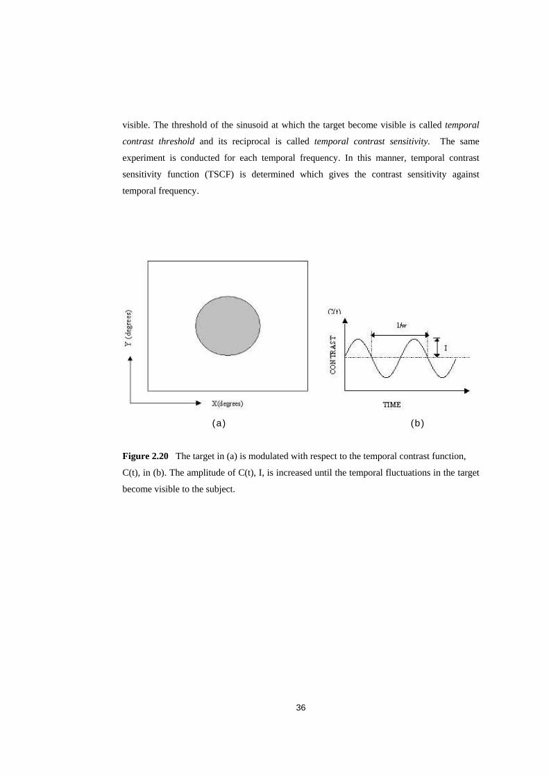
In� Figure� 2.19,� the� configuration� of� the� visual� experiment� to� find� the� temporal� contrast�
sensitivity� function� is� illustrated.� The� visual� target� (Figure� 2.20(a))� is� modulated� with� a�
sinusoidal�function,� )(tc � in�Figure�2.20(b),�and�presented�to�a�subject�standing�at�a�specific�
distance.�The�subject�is�asked�whether�the�modulated�function�target�is�distinguishable�from�
a� target�with� zero� contrast.� When� the�answer� is� negative,� the�amplitude�of� the� sinusoid� is�
increased.�The�process�is�repeated�until�the�temporal�fluctuations�in�the�visual�target�become�
�
� 36�
visible.�The�threshold�of� the�sinusoid�at�which�the�target�become�visible� is�called� temporal�
contrast threshold� and� its� reciprocal� is� called� temporal� contrast sensitivity.� � The� same�
experiment� is� conducted� for� each� temporal� frequency.� In� this� manner,� temporal� contrast�
sensitivity� function� (TSCF)� is� determined� which� gives� the� contrast� sensitivity� against�
temporal�frequency.�
�
�
�
�
� � � � � � � � � � (a)� � � � � � � � � � � � � � � � � � � � � � � � � � � � � � � � � � � � � � � � � � � � � � � � � � � � (b) �
�
Figure�2.20���The�target�in�(a)�is�modulated�with�respect�to�the�temporal�contrast�function,�
C(t),�in�(b).�The�amplitude�of�C(t),�I,�is�increased�until�the�temporal�fluctuations�in�the�target�
become�visible�to�the�subject.���
�
�

�
� 37�
�
�
�
Figure� 2.21� Temporal� contrast� sensitivity� function� of� HVS� for� different� background�
luminances.�TCSF�peaks�around�5-10�Hz.�As�the�background�luminance�increases�a�shift�to�
higher�temporal�frequencies�occurs.�[22]��
�
� TCSF� is� illustrated� in� Figure� 2.21.� � As� noted� previously,� the� size� of� the� target,�
background� luminance� and� spatial� configuration� of� the� target� affect� the� characteristics� of�
TCSF.� � Visual� experiments� show� that� an� increase� in� the� size� of� the� target� decreases� the�
sensitivity�at� low� temporal� frequencies,�while�not�affecting� the�sensitivity�at�high� temporal�
frequencies� [29].�An� increase� in� the�background� luminance�causes�a�drop�at� low� temporal�
frequency� limb� of� TCSF.� It� also� shifts� TCSF� to� higher� temporal� frequencies� [29].� A�
modification� in� the�spatial�configuration�of� the�visual� target� (Figure�2.22)�does�not�change�
the� high� frequency� limb� of� TCSF.� However,� the� presence� of� the� edges� or� high� spatial�
frequencies� in� the� target�raises�the� low�frequency� limb�of�TCSF.�Figure�2.23� illustrates�the�
effects�of�the�spatial�configuration�of�the�target�on�TCSF.���
�
�
�

�
� 38�
���������� �
�
(a)� (b)���
�
Figure�2.22�The�spatial�configurations�of�the�two�different�targets.�The�fundamental�spatial�
frequency� of� the� target� (a)� is� two� times� of� the� target� (b).� Both� of� the� two� targets� are�
modulated�with�C(t),�Figure�2.19�(b).�The�measured�TCSF�will�be�different�for�each�of�the�
visual�target.����������
�������
�
�
Figure�2.23�The�effect�of�spatial�frequency�upon�temporal�contrast�sensitivity�function.�The�
target� was� a� sinusoidal� grating� with� a� spatial� frequency� of� 0.5,� 4,� 16� or� 22cycle/degree–1�
Background�luminance�was�20�cd.m-2.�Target�was�2.5�x�2.5o�and�surround�was�10�x�10o.�The�
subjects�are�2�m.�away�from�the�visual�target.�[32]�����
�

�
� 39�
2.4.3�Temporal�Contrast�Thresholds�for �spatial�DCT�frequencies.��
�
In�image�and�video�processing,�most�of�the�compression�standards�are�based�on�block-DCT�
methods.�The�visibility�of�the�quantization�noise�in�the�DCT�domain�as�a�result�of�coding�of�
the�images�or�videos�is�of�great�concern,�since�it�affects�the�quality�of�the�image�or�video.�In�
order� to� achieve� minimum� bit� rate� with� an� acceptable� image� quality,� the� maximum�
quantization� level� that� yields� imperceptible�quantization�noise� for�human�observers�should�
be�determined.�In�[18],�optimum�quantization�levels�in�DCT�domain�for�a�given�bit�rate�are�
derived�by�a�means�of�visual�experiments�for�an�individual�image.��
� The�quantization�error�resulted�from�the�coding�of� the� images�is�a�two�dimensional�
quantity.� However,� unlike� the� images,� the� quantization� error� resulted� from� the� coding� of�
video� is� a� three� dimensional� quantity,� with� one� more� dimension,� which� is� time.� This�
quantization�error�is�called�dynamic quantization error [33].�
� The�visibility�of�the�quantization�error�as�a�result�of�the�DCT-based�coding�of�videos�
is�studied�in�[33].�The�maximum�level�of�the�dynamic�quantization�error�that�is�not�sensible�
to� HVS� is� measured.� This� maximum� level� of� dynamic� quantization� noise� is� simply� the�
temporal�contrast�threshold.��
� The� temporal�contrast� thresholds� for� the�spatial�DCT� frequencies�of� � { 0,0} ,� { 0,1} ,��
{ 0,2} ,�{ 0,3} ,�{ 0,5} ,�{ 0,7} ,�{ 1,1} ,�{ 2,2} ,�{ 3,3} ,�{ 5,5} ,�{ 7,7} �and�temporal�frequencies�of�0,�1,�
2,�4,�6,�10,�12,�15,�30�Hz.�are�measured�[33].�Figure�2.24�illustrates�the�results�for�the�spatial�
DCT� frequencies� of� { 0,0} ,� { 0,7} � and� { 3,3} .� An� increase� in� threshold� at� high� spatial� and�
temporal� frequencies� can� be� observed� easily.� The� data� in� Figure� 2.24� shows� a� low� pass�
characteristic�roughly�at�low�spatial�and�temporal�frequencies.��
� All� these� spatiotemporal� data� can� be� modeled� as� a� product� of� a� temporal�
function, )(wTw
,�a�spatial�function,� ),( vuTf
�and�an�orientation�function,� ),( vuTa
.�
�
),().,().(.),,( vuTvuTwTTwvuTafwo
= ��������������������������������������(2.10)�
�
where�o
T is�a�global�or�minimum� threshold.� )(wTw
, ),( vuTf
�and� ),( vuTa
are� illustrated� in�
Figure�2.25.�
� In� [33],� all� the� visual� experiments� to� measure� temporal� contrast� thresholds� are�
conducted�for�a�specific�purpose�of�defining�a�new�digital�video�quality�metric.�The�aim�of�

�
� 40�
such�a�metric� is�to�evaluate�visual�quality�of�digital�video.�Since�the�metric�is�based�on�the�
basics�of�HVS,�the�metric�gives�more�reliable�prediction�about�the�visual�quality�of�the�video�
when�the�observer�is�a�human.��
� In�Chapter�5,�the�temporal�contrast�thresholds�are�used�for�a�different�purpose.�The�
temporal� contrast� thresholds� are� exploited� to� determine� the� place� and� strength� of� the�
watermark�that�is�embedded�to�digital�video.����
�
�
�
Figure�2.24�Temporal�contrast�thresholds�for�spatial�DCT�frequencies�of�{ 0,0} ,�{ 0,7} �and�
{ 3,3} .��Points�are�data�of�two�observers.�The�thicker�curve�is�the�model.[33]�
�
�
�
���������������������������(a)���������������������������������������������������(b)�������������������������������������������(c)�
�
Figure�2.25�Temporal� (a),�spatial� (b)�and�orientation� (c)�components�of� the�dynamic�DCT�
threshold�model.�[33]�

�
� 41�
CHAPTER�3���
��
WATERMARKING�BASED�ON�VISUAL�MODELS������This�chapter�presents� the�basic�watermarking�methods� in� the� literature,�which�are�based�on�
perceptual�models�of�Human�Visual�System.�As�noted�in�Chapter�2,�the�models�are�derived�
by� means� of� physco-visual� experiments.� Specifically,� most� of� the� methods� presented� here�
use�the�contrast�thresholds�that�are�the�measure�of�the�sensitivity�of�HVS�for�different�spatial�
frequencies.�By�exploiting�some�characteristics�of�HVS�such�as�light�adaptation�and�contrast�
masking,� the� contrast� thresholds� are� forced� to� the� maximum� possible� level.� The� resulted�
levels� give� the� maximum� possible� watermark� strength� to� produce� visually� non-distorted�
watermarked�images.��
� In�the�first�section�of�this�chapter,�the�image�watermarking�methods�are�examined.�In�
the�second�part,�two�well-known�video�watermarking�methods�are�presented.��
�
3.1�Image�Watermarking�Methods�based�on�Visual�Models�
�
As� mentioned,� an� efficient� and� useful� watermarking� scheme� should� have� some� properties�
such�as�robustness,�capacity�and�imperceptibility�[1,2,10,11].�The�owner�of�the�image/video�
wants� to� prove� his/her� ownerships� as� long� as� the� quality� of� the� digital� content� remains.�
Hence,� the� watermark� should� be� detected� after� the� digital� content� passes� from� any� signal�
operation�that�does�not�distort�the�image�quality�considerably.�This�refers�to�robustness.�On�
the�other�hand,�the�capacity�is�directly�related�with�the�robustness.�It�refers�to�the�ability�of�
detecting� watermark� with� a� low� probability� of� error� as� the� number� of� differently�
watermarked�versions�of�an�image�or�video�increases.�Finally,�the�imperceptibility�refers�to�
visual�similarity�between�the�original�content�and�the�watermarked�content.�Obviously,�most�
of� the�owners�of�a�digital� content�do�not�want� to�any�kind�of�degradations� in� their�works.�
Therefore,� it� is� required� that� the�watermarked� image/video�have� the�same�visual�quality�as�

�
� 42�
the� original� one.� Due� to� the� mentioned� requirements,� any� researcher� working� on� digital�
watermarking�area�should�use�the�HVS�models,�which�are�mostly�developed�for� image�and�
video�coding�applications.��
� In� [34],� an� image� watermarking� method� embedding� the� watermark� by� employing�
multiresolution�fusion�technique�is�proposed.�The�method�incorporates�a�HVS�model,�which�
gives�the�contrast�sensitivity�for�a�particular�pair�of�spatial�frequencies,�as�
�
)1(.05.5),( )(1.0)(178.0 −= ++− vuvu eevuC ���������������������������������(3.1)�
�
),( vuC �is�the�contrast�sensitivity�matrix�and� u ,� v �are�the�spatial�frequencies,�given�in�units�
of� cycles� per� visual� angle.� Specifically,� in� this� method,� the� image� is� decomposed� into�
subbands�by�using�wavelet�transform�[34].�Each�subband�is�segmented�into�non-overlapping�
rectangles.�The�watermark�is�embedded�using�a�measure�called�saliency,�which�is�a�measure�
of� the� importance� of� an� image� component.� The� saliency� of� a� rectangular� segment� is�
computed� as� the� sum� of� the� product� of� the� contrast� sensitivity� function� and� square� of�
magnitude� of� the� Discrete� Fourier� transform� of� this� rectangular� segment.� This� gives� the�
measure� how� much� the� rectangular� segment� is� important� for� HVS.� If� the� importance� is�
greater,� then� the�presence�of� the�watermark�will� be� stronger� in� that� segment,� according� to�
proposed�method.�
� Another�approach�[9]�exploits�contrast�masking�and�spatial�masking�phenomenon�of�
HVS� to� guarantee� the� invisibility� of� embedded�watermark.�The� image� is�decomposed� into�
8x8�blocks�and�DCT�of�each�block�is�calculated.�A�visual�mask�is�computed�for�each�block.�
The�watermark� is�generated�scaling� the�visual�mask�and�multiplying� it�with� the�DCT�of�a�
maximal�length�pseudo-noise�sequence.�This�watermark�is�added�to�the�corresponding�DCT�
block.�Then,�the�inverse�DCT�of�each�block�into�which�watermark�is�embedded�is�computed.�
At�this�step,�spatial�masking�is�used�to�check�whether�the�watermark�is�invisible�and�control�
the�scaling�factor.�If�the�watermarking�causes�a�visible�distortion�in�the�image�block,�then�the�
scaling�factor�is�decreased�and�the�process�is�repeated.��
The�model�used�in�[9]�for�visual�mask�expresses�the�contrast�thresholds�as�a�function�
of� f ,�the�masking�frequency�m
f �and�contrast�m
c �(see�Section�2.1.2�for�the�experiments�to�
model�contrast�masking):��
��

�
� 43�
)�().(),( �])./([�,1 αmm cffkMaxfcffc
om= ������������������������������������(3.2)�
�
where� )( fco
is�detection�threshold�at�frequency� f .�The�detection�threshold�is�the�minimum�
amplitude�of�a�sinusoidal�grating�that� the�grating�can�be�discriminated�from�a�zero�contrast�
grating�(see�Section�2.1).� �In�the�case�of�8x8�DCT�transform�of�each�block,�each�frequency�
component� are� masked� by� itself� and� other� 63� spatial� frequencies.� Therefore,� a� summation�
rule� of� the� form� (3.3)� is� used� to� insert� the� affect� of� the� each� spatial� frequency� into� the�
calculation�of�contrast�threshold:�
�
ββ /1]),([)( ∑=m
f mffcfc �����������������������������������������������(3.3)�
�
where�the�value�of� β is�2.�If�the�contrast�error�between�the�original�and�watermarked�image�
is�smaller�that� )( fc ,�then�the�model�predicts�that�the�watermarked�block�is�visually�equal�to�
the�original.��
� The�spatial�model,�which� is�used� to�check� the� imperceptibility�of� the�watermark� is�
the� modified� version� of� the� Girod’s� w-model� [21].� The� w-model� predicts� spatial� and�
temporal� masking� affects� of� HVS� accurately.� � In� [23],� this� model� is� used� to� calculate� the�
tolerable error level�(TEL)�of�each�pixel�in�the�image.�If�the�resulted�error�due�to�the�image�
coding�is�larger�than�the�TEL�of�a�pixel,�the�degradation�becomes�visible�in�that�part�of�the�
image.� The� proposed� watermarking� method� [9]� also� uses� this� model� to� verify� that� the�
watermark�designed� in�DCT�domain�with� the�contrast�masking�model� is� invisible� for� local�
spatial�regions.�Each�watermark�coefficient�is�compared�with�TEL�to�assure�the�invisibility.�
If�the�watermark�coefficient�is�visible,�then�the�process�is�repeated�by�decreasing�the�scaling�
factor.��
� A� fundamental� approach� for� perceptual� watermarking� is� proposed� in� [10,11]� by�
Podilchuk,� et al.� Similar� to� � [9],� the� image� is� first� segmented� into� 8x8� non-overlapping�
blocks.� DCT� of� each� block� is� computed� and� DCT� coefficients� are� watermarked� by�
considering� just� noticeable� difference� (JND).� The� JND� is� simply� the� detection� thresholds�
measured�by�visual�experiments.�The�effects�of�luminance�masking�and�contrast�masking�are�
also� inserted� into� the� computation� of� detection� thresholds.� � The� watermarking� scheme� is�
formulated�as�follows:���

�
� 44�
>+=
�otherwise�����������������������������
�if���.
,,
,,,,,,,,,,*,,
bvu
bvubvubvubvubvubvu I
JNDIwJNDII �������������������������������(3.4)�
�
bvuI ,, is� the� DCT� coefficient� of� the� image� block� b ,� bvuJND ,, is� the� corresponding� JND�
matrix� of� the� corresponding� block� and� bvuw ,, is� the� watermark� sequence� that� is� generated�
from�zero�mean,�unit� variance�Gaussian�distribution.� In� (3.4),�only� the�coefficients�greater�
than� the�JND� levels�are�watermarked.�Since� the�coefficients� lower� than� the�JND� levels�are�
not� significant� for� HVS,� these� coefficients� are� most� probably� eliminated� after� a� possible�
compression� stage.� JND� levels� are� used� to� determine� the� strength� of� the� watermark.�
Otherwise,�the�distortion�resulted�due�to�the�watermarking�process�become�visible.�����
� Podilchuk�et al [10]�also�suggest�a�wavelet�based�watermarking�method�by�using�the�
visible� thresholds� for� each� subband� of� wavelet� transform� measured� by� means� of� visual�
experiments� (see�Table�2.1� for� the�detection� thresholds).�The�coefficients�of�each�subband�
are�watermarked�with�the�following�scheme:��
�
>+=
�otherwise�����������������������������
�if���.
,,,
,,,,,,,,,,,*,,,
flvu
flflvuflvuflflvuflvu I
JNDIwJNDII ������������������������(3.5)�
�
flvuI ,,, refers� to� the�wavelet�coefficient�at�position� ),( vu in�resolution� level� l and�frequency�
orientation� f ,� *,,, flvuI �refers�to�the�watermarked�wavelet�coefficient,� flvuw ,,, corresponds�to�
the� watermark� sequence� and� flJND , is� the� measured� just� noticeable� difference� (detection�
threshold)� for� the�subband�of�resolution� level� l and�frequency�orientation,� f.�The�reason�for�
using�such�a�watermarking�scheme�as� in�(3.5)� is� just�the�same�with�the�case�of�DCT�based�
watermarking�(3.4).�
� Podilchuk,�et al�[10]�also�make�a�comparison�between�the�DCT�based,�wavelet�based�
watermarking� methods� and� spread spectrum watermarking� method� [7].� One� of� the�
disadvantages� of� the� spread� spectrum� method� they� note� is� the� visible� distortions� in� the�
watermarked� image� for� the� case� in� which� the� original� image� contains� large� smooth� areas.�
However,� their� image�adaptive� two�different�perceptual�methods� they�proposed�give�better�
visual�results�since�the�perceptual�watermarks�adapt�on�the�local�regions�of�the�image.��

�
� 45�
� Another�novel� image�watermarking�approach� is�proposed� in� [35].�Kutter�et�al� [35]�
first�presented�the�inability�of�Weber�and�Michelson�contrast�(see�section�2.1)�to�measure�the�
contrast�of�the�natural� images.�If�one�of�these�contrast�definitions�is�used�in�natural�images,�
then�a�few�very�bright�or�dark�points�would�determine�the�contrast�of�the�whole�image.�They�
define� a� new� contrast� called� isotropic local contrast� that� is� based� on� the� Peli’s� contrast�
definition�[15]�using�the�directional�analytic�filters.�Then,�the�contrast�masking�phenomenon�
of�HVS�is�modeled�according�to�isotropic�local�contrast�by�means�of�visual�experiments�and�
the� weight� of� the� watermark� is� adjusted� according� to� this� contrast� masking� model� in� the�
watermarking�insertion�process.��
�
3.2�Video�Watermarking�Methods�based�on�Visual�Models�
�
In� contrast� to� image� watermarking,� which� is� based� on� visual� models,� the� perceptual�
watermarking�of�video�has�not�been�studied�in�detail�for�watermarking�research.�One�of�the�
reasons�of�this�fact� is�the�complexity�and�difficulty�in�modeling�of�temporal�sensitivity�and�
temporal�masking�of�HVS.�The�modeling�of�temporal�sensitivity�and�masking�phenomena�of�
HVS�is�still�an�open�research�area�[11].�
� The�video�watermarking�presents�some�other�potential�attacks�different�than�the�ones�
in�the�image�and�audio�case.�The�large�amount�of�video�data�and�high�similarity�of�frames�in�
a� scene� create� a� vulnerable� condition� for� the� attacks� such� as� frame� averaging,� frame�
dropping,�collusion�etc.�Any�method�should�be�able�to�survive�such�attacks.��
� One�simple�approach�for�video�watermarking�is�to�watermark�each�frame�of�video�as�
an� independent� image.� However,� this� case� does� not� solve� the� problem,� especially� for� the�
averaging�attack.�For�such�a�case,�an�attacker�may�average�no�motion�or�slow�motion�regions�
of� the� video� to� remove� the� watermark.� In� addition,� the� method� can� produce� visible�
distortions�in�the�watermarked�video,�since�it�is�not�based�on�the�temporal�characteristics�of�
HVS.�Moreover,�the�difference�between�the�two�consecutive�frames,�which�are�watermarked�
independently,� can� be� visible,� if� the� temporal� characteristics� of� HVS� are� not� taken� into�
account�during�the�watermark�insertion�process.��
� Unlike� the� first� case,�another�method�can�be�watermarking�of�each� frame�with� the�
same� watermark.� However,� this� method� also� poses� problems� for� the� collusion� attack.� An�
attacker� can� use� all� the� frames� in� the� video� in� order� to� detect� and� remove� that� fixed�
watermark.� Furthermore,� such� a� watermarking� process� will� be� video� independent� and� the�

�
� 46�
invisibility�of�watermark�is�not�guaranteed�for�each�video�since�the�method�is�not�based�on�
temporal�characteristics�of�HVS,�just�like�the�first�approach.��
� Podilchuk,� et al [10]� proposed� a� method� that� achieves� a� trade� off� between�
independent�watermarking�each�frame�and�utilization�of�the�same�watermark�for�each�frame.�
The�method�embeds�a�watermark�each�intra�(I)�frame�in�an�MPEG�sequence�using�the�DCT�
based� perceptual� image� watermarking� method� [10]� and� then,� apply� a� simple� linear�
interpolation� of� the� watermarks� to� every� frame� between� two� consecutive� I� frames.� If� the�
interpolation�is�not�achieved,�a�visible�distortion�is�perceived�at�each�I�frame,�while�watching�
the� video.� The� interpolation� decreases� the� visual� distortion� between� the� frames� resulted�
because� of� watermarking.� In� principle,� the� difference� between� two� consecutive� frames�
should� be� such� that� it� should� not� yield� a� distortion� greater� than� the� temporal� contrast�
thresholds�in�the�temporal�frequency�domain.��
� In�another�study� [36],�a�clever�method� is�proposed� to�solve� the�above�problems�of�
the�marking�each�frame�independently�and�using�a�fixed�watermark�for�the�entire�video.�The�
proposed�method�is�shot�based.�In�other�words,�the�video�is�separated�into�shots�and�temporal�
wavelet� transform� of� each� shot� is� computed.� A� different� watermark� is� embedded� to� each�
wavelet� coefficient� frame� by� exploiting� the� contrast� masking� and� spatial� masking�
characteristics� of� HVS.� While� the� watermarks� embedded� into� low� pass� frames� exist�
throughout�the�entire�scene,� the�watermarks�embedded�into�high�pass�frames�corresponding�
to�fast�motion�regions�of�the�video�are�highly�localized�in�time.�Such�a�watermarking�scheme�
solves� the� mentioned� problems� above.� For� example,� averaging� no� motion� or� slow� motion�
regions�of�the�video�only�distorts�the�watermark�embedded�into�high�pass�frames.�Hence,�the�
watermarks� that� are� embedded� into� low� pass� frames� survive� such� attacks.� In� addition,� the�
method�also�solves�the�collusion�attack�since�there�is�no�such�a�case�that�a�fixed�watermark�is�
embedded�to�each�frame�of�the�video.��
� One�alternative�method�of�video�watermarking�is�proposed�in�Chapter�5.�We�directly�
use� temporal� contrast� thresholds� in� our� scheme�and�show� the� robustness�of� the�method� to�
attacks� such� as� additive� Gaussian� noise,� ITU� H263+� coding,� frame� dropping� and� frame�
averaging.�
���

�
� 47�
CHAPTER�4��
�
FOVEATED�IMAGE�WATERMARKING�
�
�
The�spatial� resolution�of� the�human�visual�system�(HVS)�decreases� rapidly�away� from� the�
point� of� fixation� (foveation� point).� � By� exploiting� this� fact,� a� watermarking� approach� that�
embeds� the�watermark�energy� into� the� image�peripheral�according�to� foveation-based�HVS�
contrast�thresholds�is�presented�in�this�chapter.��
4.1 Introduction
As� already� mentioned� previous� chapters,� the� requirements� for� an� effective� watermark� are�
imperceptibility,� robustness� to� any� signal� processing� and� intended� signal� distortions,� and�
capacity� that� refers� to� the� ability� of� detecting� the� watermark� among� different� watermarks����
with�a�low�probability�of�error.�There�is�an�obvious�trade-off�between�these�requirements;�a�
gain� from� imperceptibility�will� likely� to�be� lost� from�capacity�or� robustness,�or�vice�versa.�
The�imperceptibility�criterion�is�directly�and�the�other�two�are�indirectly�related�with�human�
visual�system (HVS).�Hence,�the�researchers�working�on�digital�watermarking�usually�utilize�
visual�models,�which�are�developed�in�the�context�of�image�coding�[3-5].�
� � In� this� chapter,� we� utilize� the� foveation� phenomenon� of� HVS.� We� first� revise� the�
fundamentals�of�foveation�that�is�developed�in�the�concept�of�foveated�image�coding�[26,�27]�
and� then� propose� a� watermarking� scheme� that� exploits� this� phenomenon.� (The� basics� of�
foveation� are� given� in� Section� 2.3� in� detailed.)� We� then� quantify� the� robustness� of� the�
algorithm� against� some� typical� attacks� by� some� simulations.� A� well-known� HVS-based�
method�[10]� is�also�compared�with�our�method.� In�addition,� the�method�is�also�adapted�for�
video.�The�robustness�of�the�method�against�ITU�H263+�coding�is�tested�and�the�method�is�
compared�with�another�HVS�based�video�watermarking�method�[11].��
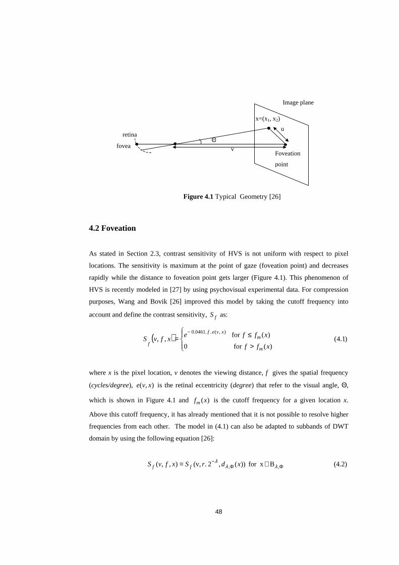
�
� 48�
�
�
�
�
�
�
�
�
�
�
4.2�Foveation��
�
As� stated� in� Section� 2.3,� contrast� sensitivity� of� HVS� is� not� uniform� with� respect� to� pixel�
locations.�The�sensitivity� is�maximum�at� the�point�of�gaze� (foveation�point)�and�decreases�
rapidly�while� the�distance� to� foveation�point�gets� larger� (Figure�4.1).�This�phenomenon�of�
HVS�is�recently�modeled�in�[27]�by�using�psychovisual�experimental�data.�For�compression�
purposes,� Wang� and� Bovik� [26]� improved� this� model� by� taking� the� cutoff� frequency� into�
account�and�define�the�contrast�sensitivity, fS as:��
( ) )1.4(������������������������������������)(for����������������������������0
)(for���,,
),(�..0461.0
>
≤=−
xff
xffexfvS
m
mxvef
f�
�
where�x� is� the�pixel� location,�v�denotes� the�viewing�distance,� f gives�the�spatial� frequency�
(cycles/degree), ),( xve is� the�retinal�eccentricity� (degree)� that� refer� to� the�visual�angle,�Θ,�
which� is� shown� in� Figure� 4.1� and� )(xfm � is� the� cutoff� frequency� for� a� given� location� x.�
Above�this�cutoff�frequency,�it�has�already�mentioned�that�it�is�not�possible�to�resolve�higher�
frequencies� from�each�other.� �The�model� in�(4.1)�can�also�be�adapted�to�subbands�of�DWT�
domain�by�using�the�following�equation�[26]:�
�
(4.2)�����������������������������B�for��x���))(,2.,(v),,( ,, ΦΦ− ∈= λλ
λ xdrSxfvS ff �
�
Figure�4.1�Typical��Geometry�[26]�
Foveation�
point�
Image�plane�
fovea�Θ�
retina�
x=(x1,�x2)�
v�
u�

�
� 49�
where� r �gives�the�display�resolution,�λ is�the�decomposition�level�of�the�wavelet�transform,�
)(, xd Φλ � is� the� equivalent� distance� of� a� wavelet� coefficient� from� the� foveation� point� at�
position� �,B�x� Φ∈ λ in�the�spatial�domain�and� Φ,Bλ is�the�set�of�wavelet�coefficient�positions�
residing� in� subband� (λ,Φ)� [26].� The� resulting� contrast� sensitivity� is� used� to� determine�
quantization�levels,�which�yield�imperceptible�quantization�error�based�on�HVS.���
�
4.3�Proposed�Watermarking�Method��
�
Let� remember� that�an� important�principle�of�watermarking� is� to�embed� the�watermark� into�
perceptually�significant�portion�of� the� image,�so� that� the� resulting� image� is�more� robust� to�
attacks�[7].�Since�perceptually�significant�part�of�the�image�is�the�region�around�the�foveation�
point,� the� watermark� should� be� embedded� mostly� into� this� part.� On� the� other� hand,� the�
strength�of�the�watermark�in�the�periphery�region�can�be�selected�higher�with�respect�to�the�
foveated�region,�since�the�contrast�threshold�levels,�which�can�be�noticed�by�HVS�are�higher�
in�those�regions.�It�will�be�shown�that�these�two�requirements�can�be�satisfied�with�a�method.��
In�the�proposed�method,�we�consider�a�similar�approach�to�conventional�HVS-based�
image�watermarking� [10,11].�Φ,λ
T ,� contrast� threshold�value� [20]� for� the�subband� level,�λ,�
and�orientation,�Φ,�in�the�DWT�domain,�is�an�important�parameter�for�these�methods,�which�
defines� the� frequency� sensitivity� of� HVS� in� different� subbands.�Φ,λ
T � is� obtained� by�
subjective�experiments�and�should�be�weighted�based�on�foveation.�Hence,�we�first�define�a
contrast threshold weight function, ),,( xfvTf ,�by�using�the�sensitivity�function� fS ,�in�(4.1):��
�
(4.3)�����������������������)(���;����)(for���������),,(/1
)(for���������),,(/1),,(
=>
≤=
fxfxffxfvS
xffxfvSxfvT
mmf
mf
f �
�
Note� that� ),,( xfvTf � is� equal� to� 1� at� the� foveation� point� and� its� value� gets� larger� as� the�
distance� from� the� foveation� point� increases.� It� reaches� to� its� maximum� at� x� = x � and� is�
assumed�to�remain�constant�after�that�point.�In�Figure�4.2,� ),,( xfvTf �is�illustrated�with�dark�
regions�showing�low�threshold�values.��

�
� 50�
�
�
�
�
�
�
�
�
�
�
�
Figure�4.2�Contrast�threshold�weight�function��(circle�center�is�the�foveation�point;�threshold�
has�its�minimum�for�dark�values)�
�
�
Using� ),,( xfvTf ,� one� may� adapt� the� contrast� threshold� weight� function� for� the�
subbands�in�DWT�domain�with�a�similar�formulation�in�(4.2):�
�
�for������))(,2.,(�),,(,, ΦΦ
− ∈=λλ
λ Bx xdrvTxfvTff
���������������������(4.4)�
�
In�order�to� include�the�effect�of�Φ,λ
T � into�the�above�formulation,� this�parameter�should�be�
multiplied� by� ),,( xfvTf � for� different� subbands� in� the� DWT� domain,� finally� giving� the�
contrast�thresholds,�as:��
�
�����������))(,2.,(.�))(,2.,( ,,, xdrvTTxdrvT f Φ−
ΦΦ− = λ
λλλ
���������������(4.5)�
�
For� the� proposed� method,� the� watermark� embedding� and� detection� processes� are�
similar� to� [5],� except� for� using� the� location� dependent� thresholds� �))(,2.,( , xdrvT Φ−
λλ
,�

�
� 51�
instead�of�constant�Φ,λ
T for�each�subband.�The�algorithm�can�be�summarized�as�follows�(for�
notational�simplicity,� �))(,2.,( , xdrvT Φ−
λλ
is�replaced�with�Φ,,λx
t ):�
1.� Decompose�image�into�multiple�subbands�using�9-7�biorthogonal�filters�[38].�
2.� Compute�Φ,, λx
t �for�each�subband�by��(4.5).�
3.� Embed�the�watermark�by�using:��
�
)6.4(�������������������������������������otherwise�������������������������������
��if�����.
,,
,,,,,,,,,,,,
*
Φ
ΦΦΦΦΦΦ
>+=
λ
λλλλλλ
x
xxxxxx
I
tIwtII �
�
where�Φ,, λx
I � is� the� wavelet� coefficient� at� position� x,� Φ,,*
λxI � is� the� corresponding�
watermarked�coefficient�and�Φ,, λx
w is�a�watermark�sequence.�����������
Figure�4.3�illustrates�the�difference�between�the�proposed�method�and�previous�HVS�
based�method�[10].�While�the�previous�method�inserts�the�watermark�according�to�Φ,λ
T ,�the�
proposed�method�embeds�the�watermark�according�to�Φ,,λx
t .�Obviously,�the�number�of�the�
watermarked�coefficients�in�the�proposed�method�is�lower�than�the�one�in�previous�method,�
while� the� strength�of� the�watermark�embedded�according� to�Φ,,λx
t � is�greater� than� the�one�
embedded�according�Φ,λ
T .�Since,�Φ,,λx
t �increases�with�increasing�eccentricity,�the�proposed�
method�yields�more�distortions�in�the�periphery.�However,�this�distortion�is�imperceptible�for�
a�human,�gazing�to�the�fixation�point.��On�the�other�hand,�the�detection�of�such�a�watermark�
obviously� improves� since� the� overall� watermark� energy� is� greater� than� the� previous� case.�
Moreover,�the�coefficients,�which�are�greater�than�a�threshold,�usually�belong�to�perceptually�
significant�portions.�
�
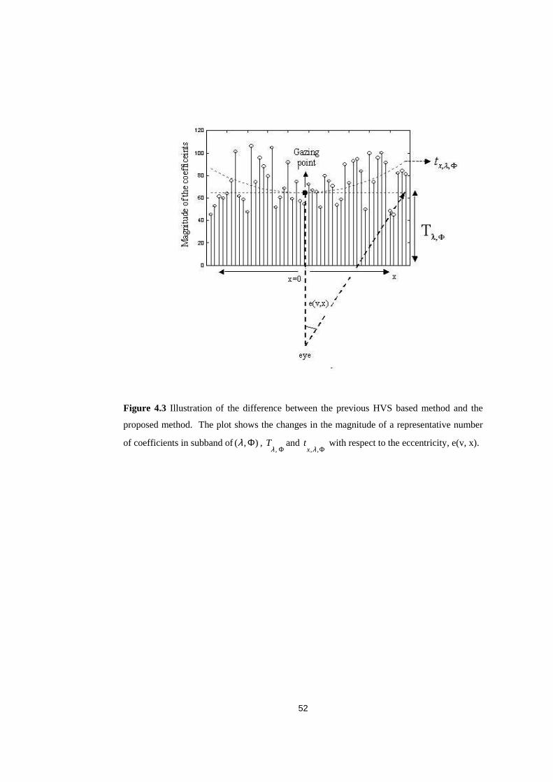
�
� 52�
�
Figure�4.3� Illustration�of� the�difference�between� the�previous�HVS�based�method�and� the�
proposed�method.��The�plot�shows�the�changes�in�the�magnitude�of�a�representative�number�
of�coefficients�in�subband�of ),( Φλ ,�Φ,λ
T and�Φ,,λx
t �with�respect�to�the�eccentricity,�e(v,�x).��
�
�
�
�
�
�
�
�
�
�
�

�
� 53�
�
4.4�Adaptation�of�the�Method�to�Video�
�
First�approach�for�adapting�the�method�to�the�video�is�to�watermark�the�each�frame�by�using�
the�proposed�method�for�images.��However,�if�performed,�the�resulting�video�will�have�some�
temporal�degradation,�such� that�a�human�observer�can�differentiate� the�original�video� from�
the�watermarked�one.��The�reason�for�the�visible�temporal�degradations�in�the�watermarked�
video�is�due�to�the�change�of�contrast�threshold�values�in�the�spatial�domain�because�of�the�
temporal�masking�phenomena�of�HVS� [11].� In�order� to�overcome� the�mentioned�problem,�
the�watermark�can�be�embedded�only� intra�frames�of�the�video.��The�other�frames�between�
every�intra�frame�pair�are�watermarked�by�making�linear�interpolation�in�the�spatial�domain�
between� these� two� watermarks,� which� are� embedded� into� the� intra� frames� [11].� The�
difference� between� any� two� frames� will� be� smaller� after� such� an� interpolation� and� hence,�
HVS�cannot�differentiate�the�degradations�in�the�video.��
�
4.5�Exper imental�Results��
�
In�all�the�simulations,�the�contrast�thresholds,�which�are�given�in�[20],�are�utilized.�For�all�the�
images,� a� single� foveation� point,� which� is� the� center� of� the� image,� is� assumed.� The�
watermark�signal�is�generated�from�a�zero�mean,�unit�variance,�Gaussian�distribution.�
� The�watermarking�detection�is�based�on�classical�detection�theory.�This�is�the�same�
approach� in� [7,10,11].� The� original� signal� is� subtracted� from� the� received� image,� and� the�
normalized� correlation� between� the� signal� difference� and� the� original� watermark� is�
computed.� First,� the� original� watermark� and� extracted� watermark� is� normalized� to� unit�
magnitude� and� then,� the� inner� product� between� them� is� computed� [40].� The� result� is�
compared� to� a� threshold.� If� the� result� is� greater� than� the� threshold,� then� the� watermark� is�
detected.� Otherwise,� the� watermark� is� not� detected.� The� reason� of� using� normalized�
correlation� is� its� robustness�against�attacks�such�as�changing�the�brightness�of� images�[40].�
With� such� a� method,� the� correlation� result� becomes� less� dependent� to� the� magnitudes� of�
original�and�extracted�watermark.������������
A� typical� result� for� Lena� image� is� given� in� Figure�4.4� (b).� The� region�around� the�
foveation� point� for� the� original� and� watermarked� images� are� shown� in� Figure� 4.4(c)� and�
Figure�4.4(d),� respectively,� in�order� to�present� the�perceptual�equivalence�of� these� regions.�

�
� 54�
The�periphery�regions�in�the�watermarked�image�are�degraded,�as�expected,�due�to�the�larger�
thresholds� in� those�regions� (see�Figure�4.4(e)�and�Figure�4.4(f)).�An� interesting�example� is�
given�in�Figure�4.5�for�the�Peppers�image.�Although�the�strength�of�the�watermark�is�higher�
in� the� periphery,� it� is� not� possible� to� sense� the� difference� between� the� original� and�
watermarked� image�even� if�a�viewer�gazes� to� the�periphery.� �For�Lena, Harbour,�Peppers,
Airfield�and�Bridge images,�the�correlation�results�against�cropping,�additive�Gaussian�noise�
with� different� variances� and� JPEG� compression� are� tabulated� in� Table� 4.1,� 4.2� and� 4.3,�
respectively.� In�order� to�determine�a� threshold� level� to�detect� the�watermark,� the�extracted�
watermark�is�correlated�with�1000�other�randomly�generated�watermarks,�in�a�similar�way�as�
in�[10].�It�should�be�noted�that�the�resulting�correlation�coefficients�are�between�0.17�and�–
0.17� for� the�Lena image.�The� results�show� that� the�watermark�can�be�detected�even� in� the�
cases�of� JPEG�compression�of� quality� 0.05,� cropping�of� 1/16�and�additive�Gaussian�noise�
resulting�PSNR�of�14�dB�between�images.�
� The�wavelet-based�watermarking�method�proposed�in�[10]�is�also�implemented�for�a�
comparison.� The� robustness� tests� of� the� wavelet-based� method� [10]� against� cropping,�
additive� Gaussian� noise� and� JPEG� compression� are� also� shown� in� Table� 4.1,� 4.2� and� 4.3,�
respectively.�The�results�indicate�a�better�performance�for�the�proposed�method�against�[10],�
in�terms�of�correlation.�For�the�proposed�method,�the�trade-off�between�the�imperceptibility�
and�the�robustness�is�managed�by�using�the�foveation�phenomena�of�HVS.��
For� the� video� simulations,� carphone.qcif� sequence� is� used.� The� robustness� of� the�
proposed�method�against� ITU�H263+�coding� standard� is� tested.�The�watermarked�video� is�
passed� through� a� H263+� coding� at� different� bit� rates.� The� results� both� for� the� proposed�
method�and�the�compared�method�[11]�are�given�in�Table�4.4.�
As�the�simulation�results�indicate,�foveation�phenomena�of�HVS�can�be�successfully�
applied� to� watermarking� for� improving� the� robustness.� Simulation� results� also� show� that�
foveation� based� watermarking� yields� an� improvement� over� previous� HVS-based�
watermarking� methods.� The� real� benefit� of� foveated� watermarking� should� be� expected� for�
video�watermarking.�
�
�
�
�
�

�
� 55�
�
�(a)�Original�image� �����������(b)�Watermarked�image�
�
�(c)��Foveated�region�in�a����������������(d)�foveated�region�in�b�
�
�(e)�periphery�region�in��(a)���������(f)�periphery�region�in�(b)�
�Figure�4.4:��original�image�and�watermarked�image��according�to�proposed�method.�
�
�

�
� 56�
�
(a)�
�� �
(b)� � � � (c)�
�
(d)� (e)�
Figure�4.5:� � (a)�original� image,� (b)�watermarked� image�according� to�proposed�method,� (c)�
watermarked� image� according� to� previous� HVS� based� method� [10],� (d)� the� amplified�
difference�image�between�(a)�and�(b),�(e)�the�amplified�difference�image�between�(d)�and�(e).��
The� brighter� points� in� the� periphery� of� (d)� compared� to� (e),� is� due� to� the� strength� of� the�
watermark,�which�is�embedded�according�to�foveation-based�thresholds.

�
� 57�
�
�
�
Cropping� Algorithm Lena� Harb� Pepp� Airf� Brid�
Proposed� 0.97� 0.89� 0.95� 0.87� 0.88�1/4�
IA-W�[11]� 0.65� 0.55� 0.54� 0.56� 0.50�
Proposed� 0.69� 0.64� 0.77� 0.54� 0.61�1/16�
IA-W�[11]� 0.33� 0.33� 0.30� 0.31� 0.25�
�
Table��4.1:�Correlation�Results��Against�Cropping.�(�¼�of�the�watermarked�image�is�cropped.�
In�the�detection�process,�the�rest�of�the�image�is�completed�with�the�original.)�
�
�
PSNR�(dB)�of�resulting�image�“Lena” �image� 14� 17� 20� 25� 31� 37� 40�
�Proposed�� 0.30� 0.47� 0.56� 0.78� 0.92� 0.98� 0.99�
IA-W�[11]� 0.19� 0.31� 0.40� 0.63� 0.79� 0.83� 0.96�
���������������
Table�4.2:�Correlation�Results�Against�Additive�Gaussian�Noise.�
�
�
Quality�factor���Image� Algorithm�
80� 60� 40� 20� 10� 5�
Proposed�� 0.89� 0.87� 0.85� 0.68� 0.58� 0.34�Lena�
IA-W�[5]� 0.70� 0.66� 0.62� 0.50� 0.30� 0.16�
Proposed� 0.98� 0.97� 0.93� 0.82� 0.55� 0.30�Harb�
IA-W�[5]� 0.95� 0.89� 0.79� 0.54� 0.31� 0.16�
Proposed� 0.98� 0.97� 0.95� 0.84� 0.58� 0.30�Pepp�
IA-W�[5]� 0.95� 0.90� 0.81� 0.53� 0.27� 0.14�
Proposed� 0.98� 0.96� 0.93� 0.83� 0.57� 0.22�Airf�
IA-W�[5]� 0.94� 0.88� 0.78� 0.55� 0.32� 0.19�
Proposed�� 0.98� 0.97� 0.95� 0.86� 0.66� 0.35�Brid�
IA-W�[5]� 0.96� 0.89� 0.81� 0.56� 0.30� 0.16�
�
Table�4.3:�Correlation�results�against�JPEG�compression�[10].�
��������������

�
� 58�
����������� �
�
�
�
�
Tab
le��4
.4�:�
Cor
rela
tion�
resu
lts�a
gain
st�I
TU
�H26
3+�c
odin
g�at
�dif
fere
nt�b
it�ra
tes.
�IA
-W:�H
VS�
base
d�vi
deo�
wat
erm
arki
ng�
met
hod�
�pro
pose
d�in
�[11
].��T
he�r
esul
ts��a
re�g
iven
�for
�Car
phon
e�se
quen
ce.�

�
� 59�
CHAPTER�5�
�TEMPORAL�WATERMARKING�OF�DIGITAL�VIDEO��
����This� chapter� presents� a� watermarking� approach� to� embed� copyright� protection� into� digital�
video.� The� approach� requires� the� original� video� to� detect� the� watermark� and� exploits�
temporal� contrast� thresholds� to� determine� the� location� where� the� watermark� should� be�
embedded� and� the� maximum� strength� of� the� watermark,� which� still� gives� imperceptible�
distortion�after�watermark�insertion.�
�
5.1�Introduction��
�
In�section�3.2,�the�problems�encountered�in�video�watermarking�are�discussed.�Briefly,�there�
are�two�main�problems�in�video�watermarking�that�makes�the�situation�different�from�image�
watermarking.� The� first� one� is� to� guarantee� the� robustness� against� attacks� such� as� frame�
dropping,� frame� averaging,� collusion� etc.� Such� attacks� have� no� counterparts� in� image�
watermarking� case.� The� second� one� is� to� provide� the� imperceptibility� of� the� watermark,�
which� is� a� relatively� more� difficult� problem� compared� to� the� image� case� due� to� the� three�
dimensional� characteristics� of� video.� The� watermarking� procedure� should� also� take� the�
variations�in�the�temporal�direction�into�account�to�provide�an�imperceptible�watermark.�Two�
solutions�in�the�literature,�which�are�based�on�HVS,�are�also�given�in�Section�3.2.�
� In�this�chapter,�we�propose�an�alternative�method�that�exploits�the�temporal�contrast�
thresholds�of�HVS.�For�a�grating�of�a�specific�spatial�frequency,�temporal�contrast�threshold�
refers�to�the�minimum�level�of�the�amplitude�of�the�sinusoidal�function�of�a�specific�temporal�
frequency,� when� the� temporal� variations� in� the� visual� target� become� visible� (see� Figure�

�
� 60�
2.20).�Therefore,�by� the�definition,� the�modifications,�which�are�smaller� than� the� temporal�
contrast� threshold� in� the� temporal�direction�of� the� target,�will�be� invisible.� In�other�words,�
temporal� contrast� thresholds� determine� the� maximum� level� of� the� watermark� that� will� be�
embedded�into�the�video�towards�temporal�direction.��
� In�Section�2.4,�temporal�contrast�thresholds�are�denoted�as� ),,( wvuT .�This�notation�
shows� the� temporal� contrast� threshold� where� the� visual� target� presented� to� a� subject� is� a�
grating� of� spatial� DCT� frequency� of� ),( vu � modulated� in� the� temporal� direction� with� a�
sinusoidal�function�of�temporal�frequency,� w .�These� ),,( wvuT thresholds�are�determined�in�
[33].� In� order� to� exploit� this� data,� the� video� should� also� expressed� as� a� function� spatial�
frequencies� ),( vu �and�temporal�frequency� w .�In�other�words,�the�video�should�be�converted�
from� ),,( tyx � domain,� where� ),( yx notates� the� spatial� horizontal� and� vertical� direction,�
respectively�and� t notates�temporal�direction,�to�the�transform�domain, ),,( wvu .�This�can�be�
interpreted�as�decomposing�the�video� into�spatiotemporal�frequency�components.�While�the�
first� component,� 0=w ,� (DC� component)� corresponds� to� the� average� of� the� video� in� the�
temporal� direction,� the� components� with� lower� wvalues� correspond� to� no� motion� or� little�
motion�regions�of�video�and�finally,�higher� w �values�correspond�to�the�high�motion�regions�
of�the�video.�Our�proposed�method�designs�the�video�watermark�according�to� ),,( wvuT and�
embeds�the�watermark�to�each�of� those�frequency�components.�With�such�an�approach,�the�
watermark�embedded�into�the�low�frequency�components�exist� throughout� the�videos�scene�
and�whereas�the�data�embedded�into�the�high�frequency�components�are�highly�localized�in�
time�and�change�rapidly�from�frame�to�frame.�����
Such�a�method�is�expected�to�eliminate�the�stated�problems�of�video�watermarking.�
Embedding�the�watermark�into�video�using�temporal�contrast�thresholds�solves�the�problem�
about� invisibility.� In�addition,� the�proposed�method�is�expected�to�be�robust�against�attacks�
such�as�averaging�of�regions�without�motion,�since�all�of�these�regions�correspond�to�the�first�
(DC)�frame�of�the�temporal�Fourier� transform�of�the�video�in�which�only�one�watermark�is�
inserted� into� this� (DC)� frame.� The� proposed� method� is� also� expected� to� be� robust� against�
attacks�like�frame�dropping�and�frame�averaging,�since�these�attacks�distort�mainly�the�high�
frequency� components� of� the� video� and� do� not� affect� low� frequency� components�
considerably.�Hence,�the�watermark�embedded�into�the�low�frequency�components�survives�
such�attacks.�Finally,� the�problem�about�the�collusion�attack� is�also�solved�by�the�proposed�
method,�since�none�of�the�frames�include�the�same�watermark,�when�the�watermark�insertion�
is�made�in�the� ),,( wvu �transform�domain.���

�
� 61�
5.2�Watermarking�Procedure��
�
The�overall�structure�of�the�watermarking�procedure�is�given�in�Figure�5.1.�The�first�step�is�
to�separate�the�video� into�shots.�Shot� is�defined�as�continuous�recording�of�a�single�camera�
[39].� �For�each�shot,� the� intensities�are�converted�into�contrast�values.��As�noted�in�Section�
2.4,� the� contrast� is� defined� as� the� ratio� of� the� target� intensity,� ),,( tyxIT
,� to� background�
intensity,� BI :�
�
B
T
I
tyxItyxC
),,(),,( = ����������������������������������������������������������(5.1)�
�
The�background�intensity,� BI ,�is�the�time-space�average�of�the�video�scene.� ),,( tyxC can�be�
written�as:��
�
)),,((
)),,((),,(),,(
tyxImean
tyxImeantyxItyxC
−= �����������������������������������������(5.2)�
�
After�this�point,�one�has�a�contrast�video,� ),,( tyxC ,�rather�than�intensity�video,� ),,( tyxI .�
�
�
�
�
�Figure�5.1�Overall�structure�of�the�watermarking�process.�

�
� 62�
),,( tyxC �should�be�transformed�to� ),,( wvu �domain�to�exploit�the�temporal�contrast�
thresholds� ),,( wvuT .�For� this�purpose,�each� frame�of� ),,( tyxC � is�divided� into�8x8�blocks�
and�DCT�of�each�block�is�calculated.�The�signal�at�this�point� is�defined�as� ),,,,( tvubybxC �
where�bx�and�by�are�the�number�of�blocks�in�horizontal�and�vertical�direction,�respectively,�u�
and�v�are�horizontal�and�vertical�spatial�frequencies,�respectively�and�t�is�time.�The�next�step�
is�to�take�the�Fourier�transform�of� ),,,,( tvubybxC �in�temporal�direction,�which�will�result�as�
),,,,( wvubybxC .��
� An� important� criterion� while� embedding� the� watermark� into� digital� content� is� to�
embed�the�watermark�into�the�perceptually�significant�part.�Since�most�of�the�common�signal�
processing�and�geometric�attacks�affect�perceptually�insignificant�parts�of�the�digital�content�
[7],�such�an�approach�makes�the�watermark�more�robust.� In�this�case,� the�digital�content� is�
video� and� perceptually� significant� parts� are� represented� by� the� coefficients� of�
),,,,( wvubybxC � which� are� greater� than� the� temporal� contrast� thresholds,� ),,( wvuT .� The�
smaller�coefficients�are�not�significant,�since�HVS�will�not�sense�them�and�probably,� these�
parts� will� be� eliminated� with� any� lossy� compression� such�as� ITU� H263+� or�MPEG� video�
coding�standards.�
� One� other� important� point� during� the� watermark� insertion� is� to� take� the� trade-off�
between� robustness� and� imperceptibility� into� account� [7].� An� increase� in� the� robustness�
performance� might� yield� a� decrease� in� imperceptibility.� In� order� not� to� affect� the�
imperceptibility� of� the� watermark,� its� strength� should� not� exceed� the� temporal� contrast�
thresholds.��
� By�using�these�two�facts,�the�watermark�insertion�is�described�by�the�relation,�as�
�
)3.5(otherwise��������������������������������������������),,,,(
),,(�),,,,(�if��),,().,,,,(),,,,(),,,,(*
≥+
=wvubybxC
wvuTwvubybxCwvuTwvubybxWwvubybxCwvubybxC �
�
where� ),,,,(* wvubybxC �denotes�the�watermarked�coefficients�and� ),,,,( wvubybxW � is�the�
watermark� sequence.� As� it� can�be� observed� from� (5.3),� the�watermark� is� inserted� into� the�
magnitude� of� the� transform� coefficients� only.� The� lower� row� of� (5.3)� satisfies� the� first�
criterion�that�is�to�embed�the�watermark�into�significant�part�of�the�video.�The�upper�row�of��
(5.3)� satisfies� the� requirement� that� the� strength� of� the� watermark� should� not� exceed� the�
temporal� contrast� thresholds� in� order� to� be� invisible,� provided� that� the� absolute� value� of�

�
� 63�
),,,,( wvubybxW �is�not�greater�than�1.�However,�if�the�watermark�is�chosen�uniformly�from�
a� restricted� interval,� e.g.,� [-1,1],� then� the� watermark� will� be� so� vulnerable� to� multiple-
document�(collusion)�attacks.��
The� multiple-document� attack� can� be� described� as� using� multiple� watermarked�
copies� '
1D ,� '
2D … '
tD � of� document� D � to� produce� an� unwatermarked� document *D � [7].� In�
order�to�eliminate�this�problem,�the�watermark�is�generated�from�a�zero�mean,�unit�variance�
Gaussian� distribution� and� temporal� contrast� thresholds� are� divided� into� the� mean� of� the�
maximum�values�of� the�1000�watermark� that� are� in� size�176�x� 144� (the� frame�size�of� the�
QCIF� sequences).� � � In� this�manner,� the�watermark�signal�will�be�mostly� lower� than�1�and�
added�signal�to�the�video�will�not�exceed�the�contrast�thresholds�so�much.��
�
5.3�Watermark�Detection���
�
The� overall� structure� of� the� watermark� detection� process� is� illustrated� in� Figure� 5.2.� The�
detection� is� based� on� the� calculation� of� normalized� correlation� between� the� original�
watermark� and� extracted� watermark� from� the� video� which� has� passed� from� some� signal�
processing�operations,�such�as�additive�Gaussian�noise,�video�coding,�frame�dropping,�frame�
averaging�etc.�The�normalized�correlation�compared� to�a� threshold.� If� it� is�greater� than� the�
threshold,� then� the� watermark� is� assumed� to� be�detected.�Otherwise,� the� watermark� is� not�
detected.��
One� of� the� important� points� while� determining� the� threshold� level� is� the� false�
positive�and� false�negative�probability.�A� false�positive�occurs�when�a�watermark�detector�
indicates� the� presence� of� a� watermark� in� an� unwatermarked� video.� A� false� positive�
probability�is�the�likelihood�of�such�an�occurrence�[40].�On�the�other�hand,�a�false�negative�
occurs�when�a�watermark�fails�to�detect�a�watermark�that�is�present�[40].�When�the�threshold�
level� is� increased,� the� false� negative� probability� decreases,� whereas� the� false� positive�
probability� increases.� Therefore,� the� threshold� level� is� determined� by� taking� the� trade-off�
between�the�false�positive�and�false�negative�probabilities�into�account.�In�order�to�determine�
such�threshold�level,� the�correlation�is�calculated�for�both�watermarked�and�unwatermarked�
cases.�The�process� is� repeated�significant� times�and� the�minimum�of� the�correlation�results�
for� the� watermarked� video� case� and� the� maximum� of� the� correlation� results� for� the�
unwatermarked�video�case�are�determined.�These�two�levels�should�be�separated�from�each�
other�as�far�as�possible,�in�order�to�survive�from�false�positive�and�false�negatives.�

�
� 64�
In� the� watermark� detection� process,� the� watermarked� video,� which� has� passed�
through�some�signal�processing�operations,�is�separated�into�shots�and�video�signal�for�a�shot�
is�notated�as� ),,(* tyxI .�The�aim�is�to�extract�the�watermark�from� ),,(* tyxI .��
�
�
(a)
(b)�
�Figure�5.2�Overall�structure�of�the�watermark�detection�process.��
������������
The� first� step� in� the� detection� process� is� to� convert� ),,(* tyxI � into� the� transform�
domain�where�the�watermark�is�inserted.�Figure�5.2�(a)�illustrates�this�case.�The�transformed�
signal� is� notated� as� ),,,,(* wvubybxC .� ),,,,( wvubybxC � is� subtracted� from�
),,,,(* wvubybxC and� the� difference� is� divided� by� ),,( wvuT .� In� mathematical� terms,� the�
operation�is�as�follows.��
),,,,(),,,,(*),,,,( wvubybxCwvubybxCwvubybxD −= �(5.4)�
),,(
),,,,(),,,,(*
wvuT
wvubybxDwvubybxW = �
�
),,,,(* wvubybxW is� the� extracted� watermark� and� normalized� correlation� between�
),,,,(* wvubybxW �and� ),,,,( wvubybxW should�be� found.�The�correlation� is� first� found� for�
each�discrete�frequency� wand�then,�the�mean�in� wdirection�is�taken:��

�
� 65�
1
),,,,(
),,,,(1
wwwvubybxW
wvubybxWv
== �
���
1
),,,,(
),,,,(
*
*
2
wwwvubybxW
wvubybxWv
=
= ���������������������������������������(5.5)�
)��and��ofproduct�inner��(i.e����.)(21211
vvvvwp = �
))(( wpmeanncorrelatio = �
�
Finally,�the�mean�is�compared�to�a�threshold�for�detection.��
��
5.4�Simulation�Results�
�
The� sequences�utilized� in� the� simulations�are� Coastguard and Carphone � sequences.�Each�
frame� is�of�174x144.�Only� first�60� frames�of� the�sequences�are�used�and� the�watermark� is�
embedded�only�Y�component.��
An� original� frame� from� each� video� is� illustrated� in� Figures� 5.3� (a)� and� 5.4� (a).��
Watermarked�frames�corresponding�to�each�one�are�illustrated�in�Figures�5.3�(b)�and�5.4�(b).�
The�PSNR�values�between�the�original�and�watermarked�frames�are�determined�as�39.9�and�
39.6,� respectively.� The� original� frame� and� watermarked� frame� are� visually� not�
distinguishable� as� illustrated.� � However,� the� visual� equivalence� of� the� watermarked� and�
original�frame�does�not�require�the�visual�equivalence�of�the�watermarked�video�and�original�
video.� As� noted,� the� differences� between� the� watermarked� video� and� original� video� can�
become� visible� due� to� the� temporal� characteristics� of� the� video.� Because� of� this� case,� the�
watermarked� video� and� original� video� are� presented� to� a� number� of� subjects� and� checked�
whether�they�sense�the�difference�between�two�videos.�According�to�these�informal�tests,�the�
videos�are�assumed�as�visually�equal.��
� According� to� motion� content� of� the� video,� the� number� of� the� coefficients� to� be�
watermarked� differs.� The� number� of� the� watermarked� coefficients� in� each� frame� of� the�
temporal� discrete� Fourier� transform� of� the� two� videos� is� illustrated� in� Figure� 5.5.� The�
numbers�of�watermarked�coefficients�are�decreasing�while�the�frequency�is�increasing.�There�
are�two�reasons�of�this�fact.�First,�the�temporal�contrast�thresholds�levels�are�increasing�while�

�
� 66�
the� temporal� frequency� is� increasing.� Second,� the� magnitudes� of� the� temporal� discrete�
Fourier� transform� of� the� videos� are� decreasing.� Due� to� these� reasons,� the� numbers� of� the�
coefficients� that� are� greater� than� the� temporal� contrast� thresholds�are� decreasing�while� the�
frequency�is�increasing.�In�Figure�5.6,�the�magnitude�of�the�difference�between�the�temporal�
discrete�Fourier�transform�magnitudes�of�the�original�and�watermarked�video�sequences�are�
illustrated� for� 4� different� discrete� frequency,� i.e.,� magnitude� of�
( ),,,,(),,,,(* wvubybxCwvubybxC − )� is� illustrated� for� 4� different� w .� As� w increases,� the�
watermarked� coefficients� are� the� ones� that� correspond� to� the� high� motion� regions� of� the�
video.� � For� the� 0=w ,� (DC� case),� most� of� the� low� spatial� frequency� elements� of� the� 8x8�
blocks�are�watermarked.�
�
�
�
(a)� � � ����������(b)��
Figure� 5.3� Frame� from� coast� video.� (a)� original� frame,� (b)� watermarked� frame.� PSNR�
between�the�watermarked�and�original�frame�is�39.9.�
�
�
�
(a)� � � ����������(b)�Figure� 5.4� Frame� from� carphone� video.� (a)� original� frame,� (b)� watermarked� frame.� Psnr�
between�the�watermarked�and�original�frame�is�39.6.�

�
� 67�
0 5 10 15 20 25 300
1000
2000
3000
4000
5000
6000
discrete�temporal�frequency
no.�
of�w
ater
mar
ked�
coef
ficie
nts
�
(a)�
0 5 10 15 20 25 300
500
1000
1500
2000
2500
3000
3500
4000
discrete�temporal�frequency
no.�
of�w
ater
mar
ked�
coef
ficie
nts
�
(b) �
Figure� 5.5� The� number� of� watermarked� coefficients� vs.� discrete� temporal� frequency� for�
coast qcif�sequence�(a),�and�carphone�qcif�sequence�(b).�Total�number�of�watermarked�qcif�
sequence�is�70270�for�the�coast sequence�and�45563�for�the�carphone sequence.���

�
� 68�
��������������� �
(a)����������������������������������������������������������(b)��
��������������� �
(c)� (d)��
Figure� 5.6� Illustration� of� where� the� watermark� are� embedded� in� the� temporal� frequency�
domain.�(a)� 0=w ,�(b)� 8=w ,�(c)� 20=w ,�(d)� 26=w �where� wshows�the�discrete�temporal�
frequency.� The� number� of� watermarked� coefficients� is� decreasing� while� w increases.� The�
plots�are�given�for�Carphone�sequence.�( w is�the�discrete�temporal�frequency�corresponding�
to�continuous�frequency�of� swN
w�.�
1−for�the�case�of�N�point�discrete�Fourier�transform�and�
sampling�frequency�of� sw .��As�noted,�N�is�60�and� sw �is�30�Hz.)�
�
�
�
�
�
�
�
�
�
�
�

�
� 69�
� During�simulations�for�the�robustness�results,�the�same�signal�processing�operation�is�
applied� both� original� and� watermarked� video.� Watermark� embedding� and� watermark�
detection� process� are� repeated� 30� times� with� different� watermarks� in� each� case.� The�
minimum�value�of�these�correlation�results,�when�watermark�is�present�in�the�video,�and�the�
maximum�value�of� the�correlation� results,�when�watermark� is� not�present� in� the� video�are�
determined.� The� larger� distance� between� that� minimum� and� maximum� values� shows� the�
robustness�of�the�system.��
�
5.4.1�Robustness�to�Additive�Gaussian�Noise��
�
In� order� to� model� video� coding� techniques� that� are� based� on� temporal� sensitivity� of� HVS�
(e.g.� such� as� 3-D� transform� coding),� the� watermarked� video� is� corrupted� with� additive�
Gaussian�noise�that�is�added�to�the�video�in�the�temporal�frequency�domain�after�multiplying�
it�with�the�temporal�contrast�thresholds:�
�
),,().,,,,(),,,,(),,,,( * wvuTwvubybxNwvubybxCwvubybxNW += �����(5.6)�
��),,,,( wvubybxNW is� the� noise� added� watermarked� coefficient,� ),,,,( wvubybxN � is� the�
additive� Gaussian� noise� with� zero� mean� and� variance� of� 0.1.� In� Table� 5.1,� the� correlation�
results�for�each�video�sequence�with�and�without�watermark�are�given.�The�maximum,�mean�
and�minimum�correlation�results�are�computed�overall�30�runs.�It�is�important�to�note�that�the����
minimum�correlation�values�with�watermark�are�much�larger�than�the�maximum�correlation�
values�without�watermark.�The�mean�of� the� inner�product� results� (see�Eqn.� (5.5))�after�30�
runs� is� drawn� as� a� function� of� discrete� temporal� frequency� in� figure� 5.7� for� each� video�
sequence�with�and�without�watermark.�It�is�clearly�seen�that�at�each�temporal�frequency,�the�
difference�between�the�correlations�for�watermarked�and�unwatermarked�case�is�quite�high.�
�
Table�5.1�Correlation�results�for�Coast�and�Carphone�sequences�after�Gaussian�noise.��
�With�watermark� Without�watermark�
Video�PSNR�
(dB)� Max� Mean� Min� Max� Mean� Min�
Coast 26.9� 0.9721� 0.9670� 0.9648� 0.0256� 0.0049� -0.0164�
Carphone 27.8� 0.9822� 0.9810� 0.9776� 0.0065� -0.0025� -0.0132�

�
� 70�
0 5 10 15 20 25 30-0.2
0
0.2
0.4
0.6
0.8
1
discrete�temporal�frequency
corr
elat
ion
�
�
Figure�5.7�Mean�of� the� inner�product� results� (see�Eqn.� (5.5))�as�a� function�of� the�discrete�
temporal� frequency� after� additive� Gaussian� noise.� The� graph� is� drawn� for� Coast� qcif�
sequence.� ‘x’s� show� � � the�correlation� results� for� the�watermarked�video�and� ‘o’s�show� the�
correlation�results�for�the�original�video.��
�
5.4.2�Robustness�to�ITU�H263�+�Coding��
�
One�of�the�most�probable�signal�processing�operations�for�video�is�a�lossy�coding�stage�that�
is�applied� for� the�purpose�of�storage�and�transmission�of�digital�video�at� low�bit� rates.�The�
robustness�of�the�watermarking�method�against�ITU�H263�+�coding�is�tested�for�different�bit�
rates.�In�the�testing�process,�one�of�each�five�consecutive�frames�is�set�as�an�intra�frame�and�
the�test�is�repeated�for�different�quantization�levels.�The�bit�rate�is�decreased�until�240�kbps�
by�increasing�the�quantization�level.�The�watermark�is�survived�until�the�bit�rate�of�230-240�
kbps.�The�correlation� results�are� illustrated� in�Table�5.2� for� the�Coastguard�and�Carphone�
sequences.���In�Figure�5.8,�the�inner�product�results�for�each�different�temporal�frequency�are�
illustrated.�While�the�inner�product�(see�(5.5))�for�the�DC�term�( 0=w )�is�very�high,�the�ones�
for� the�AC�terms�are�quite� low.�The�coding�is�distorting�mostly�AC�terms.�After�230�kbps,�
more�compression�makes�the�watermark�undetectable.��
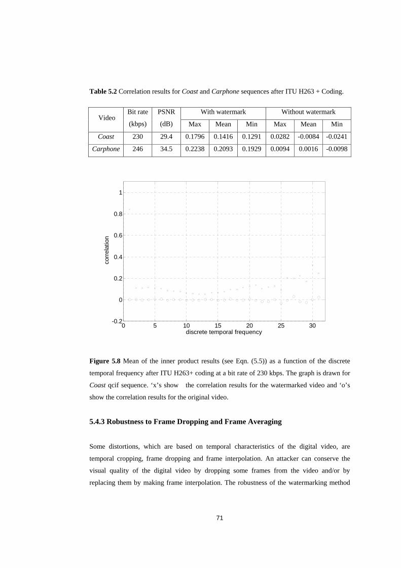
�
� 71�
Table�5.2�Correlation�results�for�Coast�and�Carphone�sequences�after�ITU�H263�+�Coding.�
�With�watermark� Without�watermark�
�Video�Bit�rate�
(kbps)�
PSNR�
(dB)� Max� Mean� Min� Max� Mean� Min�
Coast 230� 29.4� 0.1796� 0.1416� 0.1291� 0.0282� -0.0084� -0.0241�
Carphone 246� 34.5� 0.2238� 0.2093� 0.1929� 0.0094� 0.0016� -0.0098�
�
0 5 10 15 20 25 30-0.2
0
0.2
0.4
0.6
0.8
1
discrete�temporal�frequency
corr
elat
ion
�
�
Figure�5.8�Mean�of� the� inner�product� results� (see�Eqn.� (5.5))�as�a� function�of� the�discrete�
temporal�frequency�after�ITU�H263+�coding�at�a�bit�rate�of�230�kbps.�The�graph�is�drawn�for�
Coast�qcif�sequence.� ‘x’s�show��� the�correlation�results�for�the�watermarked�video�and�‘o’s�
show�the�correlation�results�for�the�original�video.�
�
5.4.3�Robustness�to�Frame�Dropping�and�Frame�Averaging��
�
Some� distortions,� which� are� based� on� temporal� characteristics� of� the� digital� video,� are�
temporal� cropping,� frame� dropping� and� frame� interpolation.� An� attacker� can� conserve� the�
visual� quality� of� the� digital� video� by� dropping� some� frames� from� the� video� and/or� by�
replacing�them�by�making�frame� interpolation.�The�robustness�of� the�watermarking�method�

�
� 72�
to�such�attacks� is� tested� in� this�part.�For� the� frame�dropping�case,�one�of�each�consecutive�
two� frames� is�dropped,�which� is� the�one�of� the�worst�case�while�probably�maintaining� the�
visual� quality.� For� the� frame� interpolation� case,� one� of� each� consecutive� two� frames� is�
dropped� and� replaced� by� the� average� of� two� neighboring� frames.� Each� of� these� attacks�
mainly� distorts� the� high� frequency� components� of� the� video.� Therefore,� only� the� low�
frequency� components� (first� 15� components)� are� taken� into� account� while� computing� the�
correlation� in� the� detection� part.� � The� correlation� results� for� frame� dropping� and� frame�
averaging� are� illustrated� in� Table� 5.3� and� 5.4,� respectively.� The� inner� product� results� vs.�
discrete�temporal�frequency�are�illustrated�in�Figure�5.9�and�5.10,�respectively,�for�the�case�
of� frame�dropping�and� frame�averaging.�Especially,� in�Figure�5.10,� the� fact� that� the� frame�
averaging�distorts�mainly�high�frequency�components�is�obvious,�since�inner�product�results�
are�decreasing�steadily�while�the�frequency�increases.���
�
�
Table�5.3�Correlation�results� for�Coast�and�Carphone�qcif�sequences�after�frame�dropping.�
One�frame�from�each�two�consecutive�frame�is�dropped.���
�
With�watermark� Without�watermark�Video�
Max� Mean� Min� Max� Mean� Min�
Coast 0.3983� 0.3925� 0.3863� 0.0079� 0.0011� -0.0072�
Carphone 0.2410� 0.2287� 0.2105� 0.0010� 0.0014� -0.0084�
�
�
Table�5.4�Correlation�results�for�Coast�and�Carphone�qcif�sequences�after�frame�averaging.�
The� odd� index� frames� are� dropped� and� replaced� by� the� average� of� the� two� neighboring�
frames.���
With�watermark� Without�watermark�Video�
Max� Mean� Min� Max� Mean� Min�
Coast 0.4295� 0.4215� 0.4127� 0.0065� -0.0016� -0.0123�
Carphone 0.2737� 0.2624� 0.2537� 0.0114� 0.0004� -0.0068�
�
�
�

�
� 73�
0 2 4 6 8 10 12 14 16-0.2
0
0.2
0.4
0.6
0.8
1
discrete�temporal�frequency
corr
elat
ion
�
�Figure�5.9�Mean�of� the� inner�product� results� (see�Eqn.� (5.5))�as�a� function�of� the�discrete�
temporal� frequency� after� frame� dropping.� One� frame� from� each� two� consecutive� frame� is�
dropped.�The�graph�is�drawn�for�Coast�qcif�sequence.�‘x’s�show���the�correlation�results�for�
the�watermarked�video�and�‘o’s�show�the�correlation�results�for�the�original�video.��
�
� �

�
� 74�
0 2 4 6 8 10 12 14 16-0.2
0
0.2
0.4
0.6
0.8
1co
rrel
atio
n
discrete�temporal�frequency�
�
Figure�5.10�Mean�of�the� inner�product�results�(see�Eqn.�(5.5))�as�a�function�of�the�discrete�
temporal� frequency�after� frame�averaging.�The�odd� index� frames�are�dropped�and�replaced�
by�the�average�of�the�two�neighboring�frames.��The�graph�is�drawn�for�Coast�qcif�sequence.�
‘x’s�show�� � the�correlation�results� for� the�watermarked�video�and� ‘o’s�show�the�correlation�
results�for�the�original�video.��
�
�
�
�
�
�
�
�
�
�
�
�
�

�
� 75�
CHAPTER�6��
��
SUMMARY�AND�DISCUSSIONS��
��Two� new� watermarking� methods,� which� consider� HVS� in� their� formulation,� have� been�
proposed�in�this�thesis:��
The�first�method,�which�is�based�on�the�foveation�phenomenon�of�HVS,�embeds�the�
watermark�into�the�periphery�with�the�assumption�that�the�human�eye�gazes�to�the�center�of�
the� image.�With�such�an�assumption,� the�visual�difference�between�original� image�and� the�
watermarked� image� cannot� be� sensed� by� HVS.� The� robustness� results� show� that� the�
watermarking� scheme� can� survive� the� attacks,� such� as� additive� Gaussian� noise,� JPEG�
compression� and� cropping.� In� addition,� it� shows� better� performance� with� respect� to� the�
previous�HVS�based�watermarking�methods.�Actually,� the� robustness� results�are�expected,�
since�more�watermarking�energy� is�embedded�into�the�periphery�regions�of�the� image.�Due�
to� this� reason,� the� overall� watermark� energy,� embedded� into� the� image� increases� and�
obviously,� detecting� the� watermark� having� more� energy� becomes� easier.� However,� the�
subjective�quality�still�does�not�change.����
One�of�the�important�points�to�note�is�assuming�the�center�point�of�the�image�as�the�
gazing�point�of�HVS.�Actually,� the�assumption� is�only�made� for�simulation�purposes.� It� is�
possible�to�extend�the�scheme�for�multiple�foveation�points,�which�is�the�more�usual�case�in�
daily�life.�While�a�person�gazes�to�point�while�watching�the�TV,�another�people�may�gazes�to�
another�point.�In�fact,�the�problem�is�not�to�extend�the�method�for�multiple�foveation�points,�
but� to� determine� the� foveation� points.� For� such� a� purpose,� it� is� possible� to� integrate� the�
watermarking�scheme�with�an�image�understanding�system.��For�example,�the�human�face�is�
likely�to�be�the�foveation�point�when�it�is�recognized�once.�It�is�also�more�likely�that�the�high�
motion�regions�attract�more�attention�than�the�slow�motion�regions�in�the�video.�Hence,�such�
an� image�understanding�system� that�determines� the�human� faces�or�high�motion� regions� in�
video,�can�be�used�before�the�watermarking�scheme.��
�
� 76�
The�second�proposed�method,�which�is�tailored�for�video�watermarking,�is�based�on�
the�temporal�sensitivity�of�HVS.�The�method�embeds�the�watermark�in�the�temporal�Fourier�
domain� by� exploiting� the� temporal� contrast� thresholds,� which� are� obtained� by� subjective�
psychovisual�experiments.� �The� robustness� results�show� that� the�watermarking�scheme�can�
survive�the�typical�video�attacks,�such�as�additive�Gaussian�noise,�ITU�263�+�coding,�frame�
dropping�and�frame�averaging.�One�interesting�point�in�the�results�is�better�robustness�of�the�
DC�term�of�video�compared�to�AC�terms,�especially�in�the�test�for�ITU�263+�coding.�While�
the�correlation�for�the�AC�terms�of�the�video�can�not�be�detected�after�the�bitrate�of�230-240�
kbps,� the� correlation� result� for� the� DC� term� can� stand� up� to� even� 50-60� kbps.� One� may�
conclude�that�the�ITU�263+�coding�distorts�mostly�the�AC�components�of�video.�
� While�testing�the�algorithms,�the�computational�complexity�of�the�algorithms�is�not�
taken� into� account,� since� the� main� application� is� assumed� as� the� copyright� protection.� As�
noted,� the� computational� cost� and� memory� requirements� are� not� a� priority� in� copyright�
protection.�The�owner�of�the�content�may�want�to�prove�his/her�ownership,�whether�it�takes�
days�to�complete�the�watermark�detection�process.�In�contrast�to�the�case,�if�the�same�idea�is�
used� in� a� broadcast� monitoring� application,� the� algorithm� should� surely� take� those�
requirements� into� account.� Although� formal� tests� are� not� performed,� the� complexity� of�
algorithms�is�not�demanding.��
� The� proposed� method� embeds� the� watermark� only� into� Y� component� of� video.�
However,�it� is�possible�to�extend�the�scheme�by�watermarking�chromatic�components.�Such�
an�approach�will�improve�the�robustness,�while�not�loosing�from�imperceptibility�due�to�low�
sensitivity�of�chromatic�components.��
� One�other�possible�extension�of�the�method�can�be�realized�with�the�use�of�temporal�
masking� phenomenon� of� HVS.� In� such� a� scheme,� the� temporal� contrast� threshold� for� a�
specific� temporal� frequency� increases� due� to� the� masking� of� a� temporal� variation� at� a�
different� temporal� frequency.�This� phenomenon�of�HVS�can�be� interpreted�as� the� contrast�
masking� in� temporal� direction.� One� may� expect� the� robustness� of� such� a� watermarking�
scheme� will� be� better� compared� to� the� proposed� method� due� to� the� increase� in� contrast�
thresholds.��
�
�
�
�
� 77�
REFERENCES��
�
[1]�����Ingemar�J.Cox,�Matt�L.�Miller�and�Jeffrey�A.�Bloom,�“Watermarking�Applications�and���
their�properties” ,�Int.�Conf.�On�Information�Technology’2000,�Las�Vegas,�2000.�
[2]� � � Gerhard� C.� Langelaar,� Iwan� Setyawan,� and� Reginald� L.� Lagendijk,� “Watermarking�
Digital�Image�and�Video�Data” ,�IEEE�Signal�Processing�Magazine,�September�2000.�������
[3]� � Maurice� Mass,� Ton� Kalker,� Jean-Paul� M.G� Linnartz,� Joop� Talstra,� Geert� F.� G.�
Depovere,� and� Jaap� Haitsma,� “ � Digital� Watermarking� for� DVD� Video� Copy�
Protection” ,��IEEE�Signal�Processing�Magazine,�September�2000.��
[4]�����Fabien�A.P.�Petitcolas,�“ �Watermarking�Schemes�Evaulation” ,�IEEE�Signal�Processing�
Magazine,�September�2000.��
[5]� � � Technical� Report,� submitted� to� � The� Scientific� and� Technical� Research� Council� of�
Turkey�(Tübitak)�under�project�EEEAG�101E007,�April�2002.���
[6]� � � �Jean�François�Delaigle,� “ �Protection�of� Intellectual�Property�of� Images�by�perceptual�
Watermarking” ,�Ph.D�Thesis�submitted�for�the�degree�of�Doctor�of�Applied�Sciences,�
Universite�Catholique�de�Louvain,�Belgique.����
[7]� � � Ingemar� J.� Cox,� Joe� Kilian,� Tom� Leighton,� and� Talal� Shamoon,� “Secure� Spread�
Spectrum� Watermarking� for� Multimedia” ,� IEEE� Trans.� on� Image� Processing,� 6,� 12,�
1673-1687,�(1997).��
[8]� � � Mitchell� D.� Swanson,� Mei� Kobayashi,� and� Ahmed� H.� Tewfik,� “Multimedia� Data-�
Embedding�and�Watermarking�Technologies” ,�Proceedings�of�the�IEEE.,�Vol.�86,�No.�
6,�June�1998.�
[9]�����Mitchell�D.�Swanson,�Bin�Zhu,�and�Ahmed�H.�Tewfik,�“Transparent�Robust�Image�
Watermarking” ,�1996�SPIE�Conf.�on�Visual�Communications�and�Image�Proc.�
[10]���Christine�I.�Podilchuk�and�Wenjun�Zeng,�“ �Image-Adaptive�Watermarking�Using�
Visual�Models” ,�IEEE�Journal�of�Selected�Areas�in�Communications,�Vol.16,�No.4,�
May�1998.��
�
� 78�
[11]���Raymond�B.�Wolfgang,�Christine�I.�Podilchuk�and�Edward�J.�Delp,�“Perceptual�
Watermarks�for�Image�and�Video” ,�Proceedings�of�the�IEEE,�Vol.�87,�No.�7,�July�
1998.��
[12]���Sergio�D.�Servetto,�Christine�I.�Podilchuk,�Kannan�Ramchandran,�“Capacity�Issues�in�
Digital�Image�Watermarking” ,�In�the�Proceedings�of�the�IEEE�International�
Conference�on�Image�Processing�(ICIP),�Chicago,�IL,�October�1998.�
[13]���Ingemar�J.�Cox�and�Matt�L.�Miller,�“A�review�of�watermarking�and�the�importance�of�
perceptual�modeling” ,�Proc.�of�Electronic�Imaging’97,�February�1997.�
[14]���Stefan�Winkler,�Pierre�Vandergheynst,�“ �Computing�Isotropic�Local�Contrast�from�
Oriented�Pyramid�Decompositons” ,��in�Proc.�ICIP,�Vol.�4,�PP.�420-424,�Kyoto,�Japan,�
1999.�
[15]��Eli�Peli,�“Contrast�in�Complex�Images” ,�Journal�of�optical�Society�of�America,�
A/Vol.7,�No.�10,�October�1990.���
[16]��Jae�S.�Lim, Two-dimensional Signal and Image Processing,�PP.�429-430.�Prentice�Hall,�
1990.��
[17]���T.�N.�Cornsweet,�Visual Perception, PP.�152-154.�New�York:�Academic,�1970.��
[18]� �A.B.�Watson,� “DCT�quantization�matrices�visually�optimized� for� individual� images” ,�
Proc.�of�SPIE�on�Human�Vision,�Visual�Processing,�and�Digital�Display�IV,�1993.�
[19]���G.�E.�Legge�and�J.�M.�Foley,�"Contrast Masking in Human Vision",�J.�Opt.�Soc.�Am.,�
70(12),�PP.�1458-1471,�1980.�
[20]� � A.� Watson,� G.� Yang,� J.� Solomon,� J.� Villasenor,� “Visibility� of� wavelet� quantization��
noise” ,�IEEE�Transactions�on�Image�Processing,�vol.�6,�no.8,�pp.�1164-1175,�August,�
1997�
[21]��Bernd�Girod,�“The�information�theoretical�significance�of�spatial�and�temporal�masking�
in� video� signals” ,� SPIE� Vol.� 1077� Human� Vision,� Visual� Processing� and� Digital�
Display,�1989.��
[22]���Bernd�Girod,�lecture�notes,�www.stanford.edu/class/ee392c/lectures/chapter05.pdf.��
[23]���Bin�Zhu,�Ahmed�H.�Tewfik,�Ömer�N.Gerek,�“Low�Bit�Rate�Near-Transparent�Image�
Coding,” �in�Proc.�of�the�SPIE�Int.�Conf.�on�Wavelet�Apps.�for�Dual�Use,�Vol.�2491,�
(Orlando,�FL),�PP.�173-184,�1995.�
[24]���Web�Vison�Home�Page,�http://webvision.med.utah.edu/anatomy.html�
[25]���Kimball’s�Biology�pages,�http:�//�users.rcn.com/�jkimball.ma.ultranet/�BiologyPages/�
V/�Vision.html.�

�
� 79�
[26]� � Zhou� Wang� and� Alan� Conrad� Bovik,� “Embedded� Foveation� Image� Coding” ,� IEEE�
Transactions�on�Image�Processing,�Vol.�10,�No.�10,�October�2001.���
[27]� �Wilson�S.�Geisler�and�Jeffrey�S.�Perry,� “A� real-time� foveated�multiresolution�system�
for�low-bandwidht�video�communication” ,��SPIE�Proceedings,�Vol.�3299,�1998.��
[28]���Amir�Said�and�William�A.�Pearlman,�“A�New�Fast�and�Efficient�Image�Codec�Based�
on�Set�Partitioning�in�Hierarchical�Trees” ,�IEEE�Transactions�on�Circuits�and�Systems�
for�Video�Technology,�Vol.�6,�No.3,�June�1996.����
[29]� � �Watson,�A.B.�(1986).�Temporal sensitivity.� In�Boff,�K.,�Kaufmann,�L.�&�Thomas,�J.�
(eds.),� Handbook� of� Human� Perception� and� Performance,� 1,� Chapter� 6.� New� York:�
John�Wiley�and�Sons.�
[30]� � Kelly,� D.� H.� ,� “Effects� of� sharp� edges� in� a� flickering� field” ,� Journal� of� the� Optical�
Society�of�America,�1959,�49,�730-732.��
[31]� � Roufs,� J.A.J.� � “Dynamic� properties� of� vision-I.� Experimental� relationships� between�
flicker�and�flash�thresholds” ,�Vision�Research,�1972,�12,�261-278.�
[32]���Robson,�J.G.�“Spatial�and�temporal�contrast�sensitivity�functions�of�the�visual�system”,�
Journal�of�theOptical�Society�of�America,�1966,�56,�1141-1142.��
[33]���Andrew�B.�Watson,�James�Hu,�John�F�McGowan�III,�“DVQ:�A�Digital�Video�Quality�
Metric�based�on�Human�Vison” ,�Journal�of�Electronic�Imaging,�10(1),�20-29.�
[34]� � Deepa� Kundur� and� Dimitrios� Hatzinakos,� “A� Robust� Digital� Image� Watermarking�
Method� using� Wavelet-Based� Fusion” ,� IEEE� Signal� Processing� Society� 1997�
International�Conference�on�Image�Processing�(ICIP'97).��
[35]� � Martin� Kutter� and� Stefan� Winkler,� “A� vison-based� Masking� � Model� for� Spread-
Spectrum�Image�Watermarking” ,�IEEE�Transactions�on�Image�Processing,�Vol.11,�No.�
1,�January�2002.��
[36]���Mitchell�D.�Swanson,�Bin�Zhu�and�Ahmed�H.�Tewfik,�“Multiresolution�Scene-Based�
Video� Watermarking� using� perceptual� Models” ,� IEEE� Journal� on� Selected� Areas� in�
Communications,�Vol.�16,�No.�4,�May�1998.������
[37]���M.�Ramkumar,�A.�N.�Akansu�and�A.�A.�Alatan,�“On�the�choice�of�transforms�for�data�
hiding�in�compressed�video,” �Proc.�IEEE�ICASSP�'99,�Phoenix,�pp.�3049-3052,�1999.�
[38]� � M.� Antonini,� M.� Barlaud,� P.� Mathieu� and� I.� Daubechies.� “ Image� coding� using� the��
wavelet�transform” ,�IEEE�Trans.�on�Image�Processing,�Vol.�1,�PP.�205-220,�Feb�1992.�
[39]� � A.� Aydın� Alatan,� Ali� N.� Akansu� and� Wayne� Wolf,� “Multi-Modal� Dialog� Scene�
Detection� Using� Hidden� Markov� Models� for� Content-Based� Multimedia� Indexing” ,����
Multimedia�Tools�and�Applications,�14,�137-151,2001.���

�
� 80�
[40]� � Ingemar� J.� Cox,� Matthew� L.� Miller,� Jeffrey� A.� Bloom,� Digital Watermarking,�
Academic�Press,�2002.� �
�


![[Digital Watermarking 01 & 02] Applications and Properties of Watermarking](https://img.pdfslide.net/doc/110x75/577d34c41a28ab3a6b8ecca2/digital-watermarking-01-02-applications-and-properties-of-watermarking.jpg)