Embed Size (px)
Citation preview

Diploma in StatisticsDesign and Analysis of Experiments
Lecture 4.2 1
Design and Analysis of ExperimentsLecture 4.2
Part 1: Components of Variation
– identifying sources of variation– hierarchical design for variance component
estimation– hierarchical ANOVA
Part 2: Measurement System Analysis
– Accuracy and Precision– Repeatability and Reproducibility– Components of measurement variation– Analysis of Variance– Case study: the MicroMeter

Diploma in StatisticsDesign and Analysis of Experiments
Lecture 4.2 2
An invalid comparison
Comparing standard process, A,
with modified process, B
A B
58.3 63.2
57.1 64.1
59.7 62.4
59.0 62.7
58.6 63.6
Means: 58.54 63.20
St. Devs: 0.96 0.68

Diploma in StatisticsDesign and Analysis of Experiments
Lecture 4.2 3
An invalid comparison
Process: batch manufacture of pigment paste
Key variable: moisture content
Sampling plan: single sample from single batch
Measurements: 5 repetitions
s measures measurement error
no measure of variation within batch
no measure of variation between batches

Diploma in StatisticsDesign and Analysis of Experiments
Lecture 4.2 4
Sources of variation in moisture content
• Batch, subject to Process variation
• Sample from batch, subject to within batch variation
• Measurement, subject to Test variation
Model for variation in moisture content:
Y = + eP + eS + eT

Diploma in StatisticsDesign and Analysis of Experiments
Lecture 4.2 5
Values
Values
eP
P
Sources of variation in moisture content
Processvariation
•

Diploma in StatisticsDesign and Analysis of Experiments
Lecture 4.2 6
Values
Values
eP
eS
S
P
Sources of variation in moisture content
Processvariation
Samplingvariation
•
•

Diploma in StatisticsDesign and Analysis of Experiments
Lecture 4.2 7
Values
Values
•
S
T
eP
eS
P
eT
e = eP + eP + eP
Sources of variation in moisture content
Processvariation
Samplingvariation
Testingvariation
y
•
•

Diploma in StatisticsDesign and Analysis of Experiments
Lecture 4.2 8
Components of Variance
Recall basic model:
Y = + eP + eS + eT
Components of variance:2T
2S
2P
2Y
2T
2S
2PY

Diploma in StatisticsDesign and Analysis of Experiments
Lecture 4.2 9
Conclusions for process testing
• Process measurements are subject to a hierarchy of variation sources.
• Several measurements on a single sample from a single batch do not reflect overall variation.
• Several batches and several samples from each batch are necessary to capture overall variation.
• Comparison of process methods must be referred to the relevant level of variation

Diploma in StatisticsDesign and Analysis of Experiments
Lecture 4.2 10
Hierarchical Design forVariance Component Estimation
• A batch of pigment paste consists of 80 drums of material.
• 15 batches were available for testing
• 2 drums were selected at random from each batch and a sample was taken from each drum.
• 2 tests for moisture content were run on each sample.
• The results follow

Diploma in StatisticsDesign and Analysis of Experiments
Lecture 4.2 11
Hierarchical Design forVariance Component Estimation
Batch 1 2 3 4 5 Sample 1 2 3 4 5 6 7 8 9 10 Test 40 39 30 30 26 28 25 26 29 28 14 15 30 31 24 24 19 20 17 17 Batch 6 7 8 9 10 Sample 11 12 13 14 15 16 17 18 19 20 Test 33 32 26 24 23 24 32 33 34 34 29 29 27 27 31 31 13 16 27 24 Batch 11 12 13 14 15 Sample 21 22 23 24 25 26 27 28 29 30 Test 25 23 25 27 29 29 31 32 19 20 29 30 23 23 25 25 39 37 26 28

Diploma in StatisticsDesign and Analysis of Experiments
Lecture 4.2 12
Nested ANOVA: Test versus Batch, Sample
Analysis of Variance for Test
Source DF SS MS F PBatch 14 1216.2333 86.8738 1.495 0.224Sample 15 871.5000 58.1000 64.556 0.000Error 30 27.0000 0.9000Total 59 2114.7333
Variance Components % ofSource Var Comp. Total StDevBatch 7.193 19.60 2.682Sample 28.600 77.94 5.348Error 0.900 2.45 0.949Total 36.693 6.058

Diploma in StatisticsDesign and Analysis of Experiments
Lecture 4.2 13
Nested ANOVA: Test versus Batch, Sample
Expected Mean Squares
1 Batch 1.00(3) + 2.00(2) + 4.00(1)2 Sample 1.00(3) + 2.00(2)3 Error 1.00(3)
Translation:
EMS(Batch) =
EMS(Sample) =
EMS(Error) =
2B
2S
2T 42
2S
2T 2
2T

Diploma in StatisticsDesign and Analysis of Experiments
Lecture 4.2 14
Calculation
= EMS(Error)
= ½[EMS(Sample) – EMS(Error)]
= ¼[EMS(Batch) – EMS(Sample)]2B
2S
2T

Diploma in StatisticsDesign and Analysis of Experiments
Lecture 4.2 15
Theory
Model:
Yijk = + i + i(j) + ijk
Yij. = + i + i(j) + ij.
Yi.. = + i + i(.) + i..
Decomposition:
(Yijk – Y... ) = (Yi.. – Y... ) + (Yij. – Yi.. ) + (Yijk – Yij. )
(Yij. – Yi.. ) = (i(j) – i(.) ) + (ij. – i.. )
EMS involves and
2S 2
T

Diploma in StatisticsDesign and Analysis of Experiments
Lecture 4.2 16
Conclusions fromVariance Components Analysis
Variance Components % ofSource Var Comp. Total StDevBatch 7.193 19.60 2.682Sample 28.600 77.94 5.348Error 0.900 2.45 0.949Total 36.693 6.058
Sampling variation dominates, testing variation is relatively small.
Investigate sampling procedure.
Diploma in StatisticsDesign and Analysis of Experiments
Lecture 4.2 17
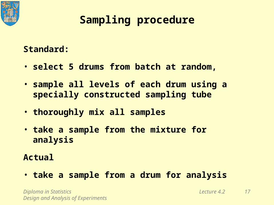
Sampling procedure
Standard:
• select 5 drums from batch at random,
• sample all levels of each drum using a specially constructed sampling tube
• thoroughly mix all samples
• take a sample from the mixture for analysis
Actual
• take a sample from a drum for analysis

Diploma in StatisticsDesign and Analysis of Experiments
Lecture 4.2 18
Another Example
Testing drug treatments for pregnant women
22 women, 10 treatment A, 7 treatment B, 5 "control".
Placentas examined for "irregularities":
5 locations,
10 slices, on microscope slides,
5 measurements (counts of "irregularities") per slide,
5,500 measurements in all.
No significant treatment effect (10 vs 7)
Diploma in StatisticsDesign and Analysis of Experiments
Lecture 4.2 19
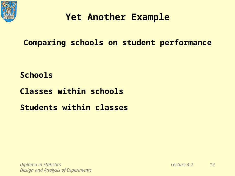
Yet Another Example
Comparing schools on student performance
Schools
Classes within schools
Students within classes

Diploma in StatisticsDesign and Analysis of Experiments
Lecture 4.2 20
Design and Analysis of ExperimentsLecture 4.2
Part 2: Measurement System Analysis
– Accuracy and Precision– Repeatability and Reproducibility– Components of measurement variation– Analysis of Variance– Case study: the MicroMeter

Diploma in StatisticsDesign and Analysis of Experiments
Lecture 4.2 21
The MicroMeter optical comparator

Diploma in StatisticsDesign and Analysis of Experiments
Lecture 4.2 22
The MicroMeter optical comparator
• Place object on stage of travel table
• Align cross-hair with one edge
• Move and re-align cross-hair with other edge
• Read the change in alignment
• Sources of variation:
– instrument error
– operator error
– parts (manufacturing process) variation

Diploma in StatisticsDesign and Analysis of Experiments
Lecture 4.2 23
Precise
Biased
Accurate
Characterising measurement variation;Accuracy and Precision
Imprecise

Diploma in StatisticsDesign and Analysis of Experiments
Lecture 4.2 24
Characterising measurement variation;Accuracy and Precision
Centre and Spread
• Accurate means centre of spread is on target;
• Precise means extent of spread is small;
• Averaging repeated measurements improves precision, SE = /√n
– but not accuracy; seek assignable cause.

Diploma in StatisticsDesign and Analysis of Experiments
Lecture 4.2 25
Accuracy and Precision: Example
Each of four technicians made six measurements of a standard (the 'true' measurement was 20.1), resulting in the following data:
Technician Data
1 20.2 19.9 20.1 20.4 20.2 20.4
2 19.9 20.2 19.5 20.4 20.6 19.4
3 20.6 20.5 20.7 20.6 20.8 21.0
4 20.1 19.9 20.2 19.9 21.1 20.0
Exercise: Make dotplots of the data. Assess the technicians for accuracy and precision

Diploma in StatisticsDesign and Analysis of Experiments
Lecture 4.2 26
Accuracy and Precision: Example

Diploma in StatisticsDesign and Analysis of Experiments
Lecture 4.2 27
Repeatability and Reproducability
Factors affecting measurement accuracy and precision may include:
– instrument
– material
– operator
– environment
– laboratory
– parts (manufacturing)

Diploma in StatisticsDesign and Analysis of Experiments
Lecture 4.2 28
Repeatability and Reproducibility
Repeatability:
precision achievable under constant conditions:
– same instrument
– same material
– same operator
– same environment
– same laboratory
Reproducibility:
precision achievable under varying conditions:
– different instruments
– different material
– different operators
– changing environment
– different laboratories

Diploma in StatisticsDesign and Analysis of Experiments
Lecture 4.2 29
Measurement Capability of the MicroMeter
4 operators measured each of 8 parts twice, with random ordering of parts, separately for each operator.
Three sources of variation:
– instrument error
– operator variation
– parts(manufacturing process) variation.
Data follow

Diploma in StatisticsDesign and Analysis of Experiments
Lecture 4.2 30
Measurement Capability of the MicroMeter

Diploma in StatisticsDesign and Analysis of Experiments
Lecture 4.2 31
Quantifying the variation
Each measurement incorporates components of variation from
– Operator error
– Parts variation
– Instrument error
and also
– Operator by Parts Interaction

Diploma in StatisticsDesign and Analysis of Experiments
Lecture 4.2 32
Measurement Differences
Part Operator Repeats Diffs Part Operator Repeats Diffs
1 1 96.3 95.4 0.9 5 1 99.4 99.9 -0.5 2 97.0 96.9 0.1 2 100.1 99.8 0.3 3 98.2 97.4 0.8 3 100.9 99.4 1.5 4 97.4 99.6 -2.2 4 100.0 99.4 0.6
2 1 95.5 95.8 -0.3 6 1 93.8 94.9 -1.1 2 96.1 96.8 -0.7 2 95.9 95.8 0.1 3 97.9 99.4 -1.5 3 96.3 98.5 -2.2 4 97.3 100.0 -2.7 4 94.5 94.5 0
3 1 102.8 100.3 2.5 7 1 86.4 85.4 1 2 101.5 101.4 0.1 2 86.8 86.7 0.1 3 102.6 104.3 -1.7 3 88.2 89.6 -1.4 4 101.9 101.9 0 4 88.6 89.0 -0.4
4 1 94.6 96.2 -1.6 8 1 90.5 90.5 0 2 97.8 95.5 2.3 2 89.1 90.2 -1.1 3 96.0 94.3 1.7 3 92.9 92.1 0.8 4 95.3 94.4 0.9 4 92.1 92.4 -0.3

Diploma in StatisticsDesign and Analysis of Experiments
Lecture 4.2 33
Graphical Analysis of Measurement Differences

Diploma in StatisticsDesign and Analysis of Experiments
Lecture 4.2 34
Average measurementsby Operators and Parts

Diploma in StatisticsDesign and Analysis of Experiments
Lecture 4.2 35
Graphical Analysis of Operators & Parts
Part
Measu
rem
ent
876543210
105
100
95
90
85
Operator
34
12
Interaction Plot

Diploma in StatisticsDesign and Analysis of Experiments
Lecture 4.2 36
Graphical Analysis of Operators & Ordered Parts
PartOrder
Meas
876543210
105
100
95
90
85
Operator
34
12
Interaction Plot, ordered by Parts

Diploma in StatisticsDesign and Analysis of Experiments
Lecture 4.2 37
Quantifying the variation
Notation:
E: SD of instrument error variation
P: SD of parts (manufacturing process) variation
O: SD of operator variation
OP: SD of operator by parts interaction variation
T: SD of total measurement variation
N.B.:
so
2E
2OP
2P
2O
2T
2E
2OP
2P
2OT

Diploma in StatisticsDesign and Analysis of Experiments
Lecture 4.2 38
Calculating sE
Part Operator Repeats ½(diff)2 Part Operator Repeats ½(diff)2
1 1 96.3 95.4 0.40 5 1 99.4 99.9 0.13 2 97.0 96.9 0.00 2 100.1 99.8 0.04 3 98.2 97.4 0.32 3 100.9 99.4 1.13 4 97.4 99.6 2.42 4 100.0 99.4 0.18
2 1 95.5 95.8 0.04 6 1 93.8 94.9 0.61 2 96.1 96.8 0.25 2 95.9 95.8 0.01 3 97.9 99.4 1.13 3 96.3 98.5 2.42 4 97.3 100.0 3.65 4 94.5 94.5 0.00
3 1 102.8 100.3 3.13 7 1 86.4 85.4 0.50 2 101.5 101.4 0.00 2 86.8 86.7 0.00 3 102.6 104.3 1.45 3 88.2 89.6 0.98 4 101.9 101.9 0.00 4 88.6 89.0 0.08
4 1 94.6 96.2 1.28 8 1 90.5 90.5 0.00 2 97.8 95.5 2.64 2 89.1 90.2 0.61 3 96.0 94.3 1.45 3 92.9 92.1 0.32 4 95.3 94.4 0.40 4 92.1 92.4 0.05
sum = 18.6 sum = 7.0
s2 = (18.6 + 7.0)/32 = 0.8
sE = 0.89

Diploma in StatisticsDesign and Analysis of Experiments
Lecture 4.2 39
Analysis of Variance
Analysis of Variance for Diameter
Source DF SS MS F P
Operator 3 32.403 10.801 6.34 0.003Part 7 1193.189 170.456 100.02 0.000Operator*Part 21 35.787 1.704 2.13 0.026
Error 32 25.600 0.800
Total 63 1286.979
S = 0.894427

Diploma in StatisticsDesign and Analysis of Experiments
Lecture 4.2 40
Basis for Random Effects ANOVA
F-ratios in ANOVA are ratios of Mean Squares
Check: F(O) = MS(O) / MS(O*P)
F(P) = MS(P) / MS(O*P)
F(OP) = MS(OP) / MS(E)
Why?
MS(O) estimates E2 + 2OP
2 + 16O2
MS(P) estimates E2 + 2OP
2 + 8P2
MS(OP) estimates E2 + 2OP
2
MS(E) estimates E2

Diploma in StatisticsDesign and Analysis of Experiments
Lecture 4.2 41
Variance Components
Estimated StandardSource Value Deviation
Operator 0.5686 0.75
Part 21.0939 4.59
Operator*Part 0.4521 0.67
Error 0.8000 0.89

Diploma in StatisticsDesign and Analysis of Experiments
Lecture 4.2 42
Diagnostic Analysis
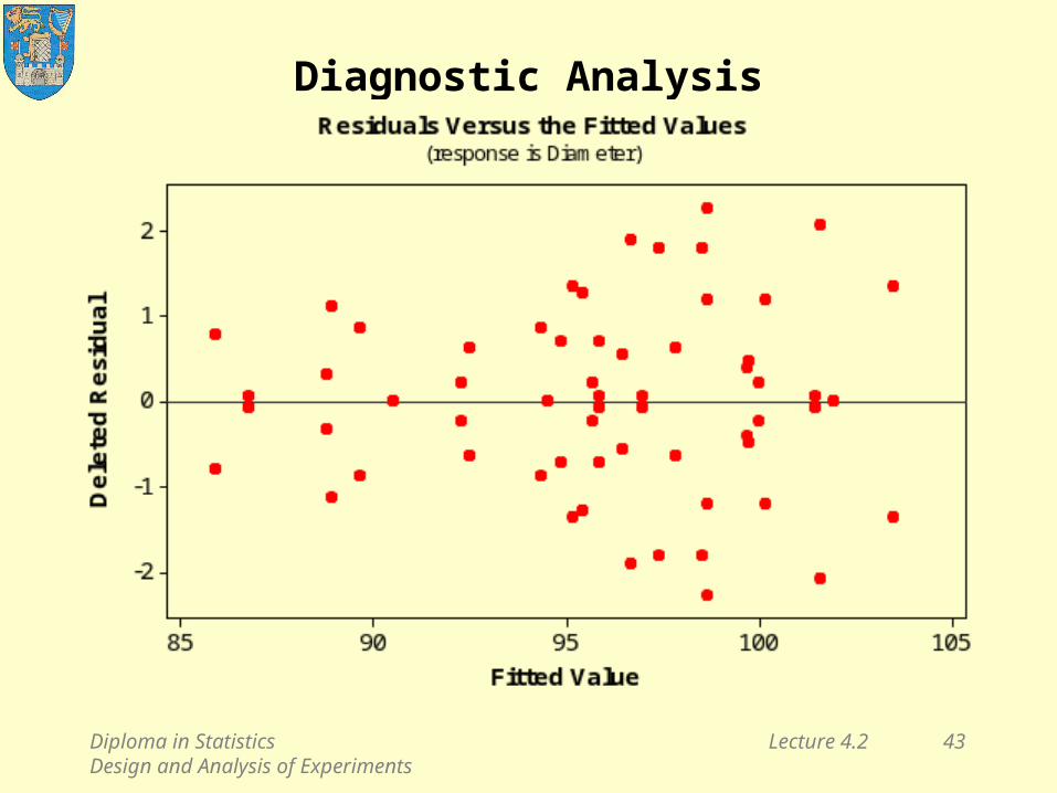
Diploma in StatisticsDesign and Analysis of Experiments
Lecture 4.2 43
Diagnostic Analysis

Diploma in StatisticsDesign and Analysis of Experiments
Lecture 4.2 44
Measurement system capability
E P means measurement system cannot distinguish between different parts.
Need E << P .
Define TP = sqrt(E2 + P
2).
Capability ratio = TP / E should exceed 5

Diploma in StatisticsDesign and Analysis of Experiments
Lecture 4.2 45
Repeatability and Reproducibility
Repeatabilty SD = E
Reproducibility SD = sqrt(O2 + OP
2)
Total R&R = sqrt(O2 + OP
2 + E2)

Diploma in StatisticsDesign and Analysis of Experiments
Lecture 4.2 46
Laboratory 1, Part 2A four factor process improvement study
Low (–) High (+)
A: catalyst concentration (%), 5 7,
B: concentration of NaOH (%), 40 45,
C: agitation speed (rpm), 10 20,
D: temperature (°F), 150 180.
The current levels are 5%, 40%, 10rpm and 180°F, respectively.

Diploma in StatisticsDesign and Analysis of Experiments
Lecture 4.2 47
Design Point
Run Order
Catalyst Concentration
NaOH Concentration
Agitation Speed
Temperature Impurity
1 2 5 40 10 150 38 2 6 7 40 10 150 40 3 12 5 45 10 150 27 4 4 7 45 10 150 30 5 1 5 40 20 150 58 6 7 7 40 20 150 56 7 14 5 45 20 150 30 8 3 7 45 20 150 32 9 8 5 40 10 180 59 10 10 7 40 10 180 62 11 15 5 45 10 180 53 12 11 7 45 10 180 50 13 16 5 40 20 180 79 14 9 7 40 20 180 75 15 5 5 45 20 180 53 16 13 7 45 20 180 54
Design and Results
Diploma in StatisticsDesign and Analysis of Experiments
Lecture 4.2 48
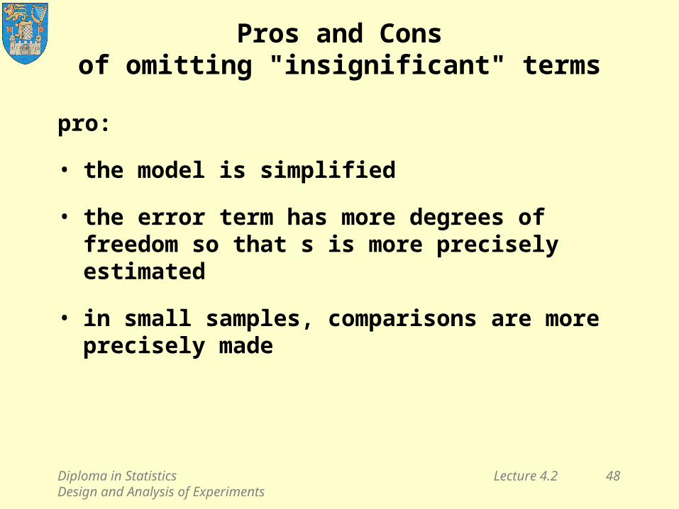
Pros and Consof omitting "insignificant" terms
pro:
• the model is simplified
• the error term has more degrees of freedom so that s is more precisely estimated
• in small samples, comparisons are more precisely made

Diploma in StatisticsDesign and Analysis of Experiments
Lecture 4.2 49
Pros and Consof omitting "insignificant" terms
con:
• statistical insignificance does not imply substantive insignificance, so that
– when the excluded term has some effect below statistically significant level, the residual standard deviation is likely to increase, giving less precise comparisons,
– (although this may be a pro if conservative conclusions are valued)
• predictions may be slightly biased.

Diploma in StatisticsDesign and Analysis of Experiments
Lecture 4.2 50
Reading
EM §1.5.3, §7.5, §8.2.1
MS Introduction to Measurement Systems Analysis
BHH, §9.3