Physikalisch-chemisches Praktikum I Dipole Moment – 2016

Dipole Moment

Summary

In this experiment you will determine the permanent dipole moments of some po-lar molecules in a non-polar solvent based on Debye’s theory and the Guggenheimapproximation. You will combine concentration-dependent measurements of refrac-tive index for visible light and of relative permittivities at radio frequencies anddevelop an understanding of the connection between these macroscopic quantitiesand molecular properties.

Contents

1 Introduction 11.1 Definition of the dipole moment . . . . . . . . . . . . . . . . . . . . . . . . 11.2 Relative Permittivity, Polarization, and Polarizability . . . . . . . . . . . . 3

1.2.1 Different Contributions to the Polarization . . . . . . . . . . . . . . 41.3 The Debye equation . . . . . . . . . . . . . . . . . . . . . . . . . . . . . . 51.4 Dispersion . . . . . . . . . . . . . . . . . . . . . . . . . . . . . . . . . . . . 61.5 Relative Permitivity and Refractive Index . . . . . . . . . . . . . . . . . . 61.6 The Guggenheim Method . . . . . . . . . . . . . . . . . . . . . . . . . . . 8

2 Experiment 82.1 The Dipole Meter . . . . . . . . . . . . . . . . . . . . . . . . . . . . . . . . 82.2 The Refractometer . . . . . . . . . . . . . . . . . . . . . . . . . . . . . . . 92.3 Measurements . . . . . . . . . . . . . . . . . . . . . . . . . . . . . . . . . . 102.4 Practical Advice . . . . . . . . . . . . . . . . . . . . . . . . . . . . . . . . . 11

3 Data Analysis 12

1 Introduction

1.1 Definition of the dipole moment

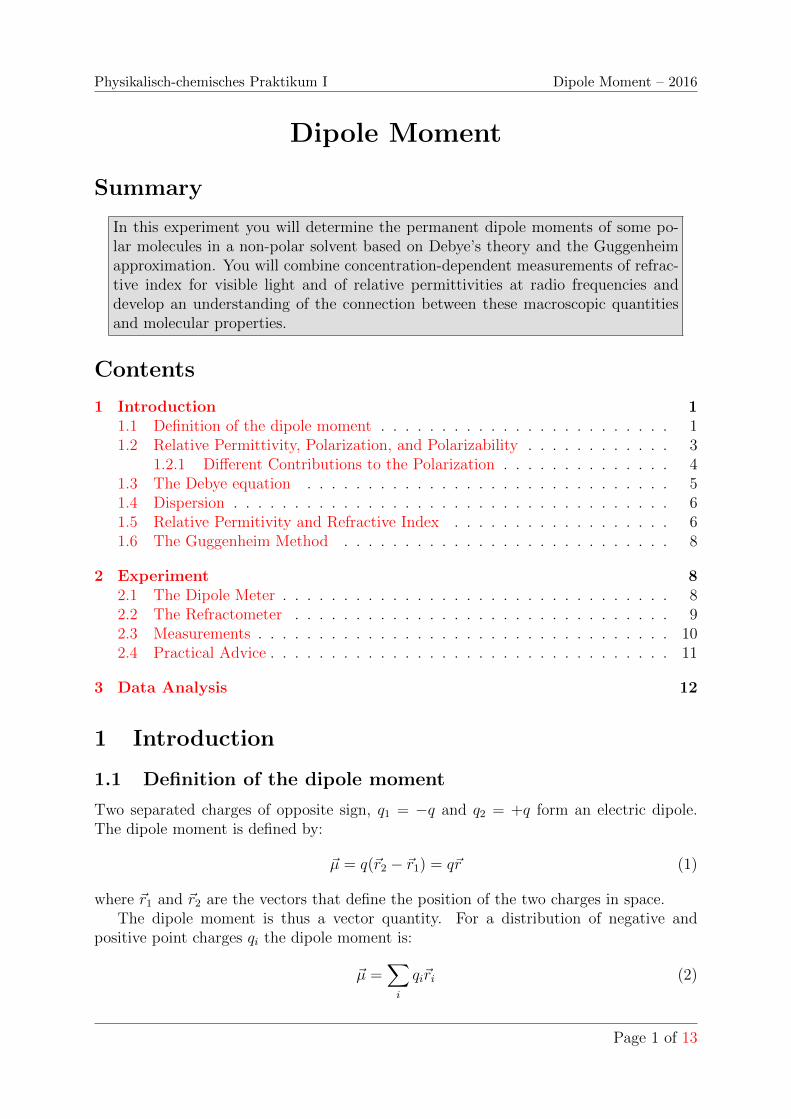
Two separated charges of opposite sign, q1 = −q and q2 = +q form an electric dipole.The dipole moment is defined by:

~µ = q(~r2 − ~r1) = q~r (1)

where ~r1 and ~r2 are the vectors that define the position of the two charges in space.The dipole moment is thus a vector quantity. For a distribution of negative and

positive point charges qi the dipole moment is:

~µ =∑i

qi~ri (2)

Page 1 of 13

Physikalisch-chemisches Praktikum I Dipole Moment – 2016

��1

��2

−�

+�

��

�(��)

��

Figure 1: Definition of the dipole moment for two point charges and a continuous charge distri-bution

where ~ri are the positions of the charges qi. For continuous charge distributions ~µ =e∫ρ(~r)~rd~r, where ρ is the charge density and e is the elementary charge. The electric

dipole moment of a molecule is the sum of the contributions of the positively chargednuclei and the negatively charged electron distribution (~µ = ~µ+ + ~µ−). The nuclei can in

good approximation be treated as point charges: ~µ+ is thus given by ~µ+ =∑N

i=1 Zie~Ri,

where Zi is the nuclear charge of nucleus i at position ~Ri. The electronic part ~µ− isdetermined by the electron distribution. It may be obtained from quantum chemicalcalculations, which yield the electronic wavefunction ψ(r) and thus ρe(~r) = |ψ(~r)|2.

In the SI system, the unit of the electric dipole moment is Coulomb·meter. Since theseunits result in very small numbers, however, the unit Debye (1D = 3.33564 · 10−30 Cm)is often used (in honor of Peter Debye, who was, from 1911-1912, professor of theoreticalphysics at the University of Zurich).

According to general convention, the dipole moment points from the center of thenegative charge distribution to the center of the positive one. If the two centers do notcoincide the molecule has a permanent dipole moment. Its existence is strongly related tothe symmetry properties of a molecule. Molecules with inversion symmetry like benzene,acetylene, or nitrogen, for instance, have no permanent dipole moment. In the case ofHCl, however, the centers of the two charge distributions do not coincide. If we placetwo elementary charges (e = 1.602 · 10−19 C) of opposite sign at a distance of 1.28 · 10−10

m, i.e. the bond length of the HCl molecule, we obtain a dipole moment of 6.14 D. Thisrepresents a purely electrostatic model for the ionic HCl structure. In practice, however,only a dipole moment of 1.08 D is found. The molecule is thus only partially ionic. Theionic character X describes partially ionic chemical bonds:

X =µexp

µcalc

· 100% (3)

for example X of HCl is 17.6%. Experimental dipole moments provide information aboutthe electron distribution in a molecule.

In this experiment dipole moments of some polar molecules in non-polar solvents aredetermined. This is done by measuring relative permittivity and refractive indices ofsolutions and pure solvents. The connection between these two macroscopic propertiesand the molecular dipole moment is explained in the following sections.

Page 2 of 13

Physikalisch-chemisches Praktikum I Dipole Moment – 2016

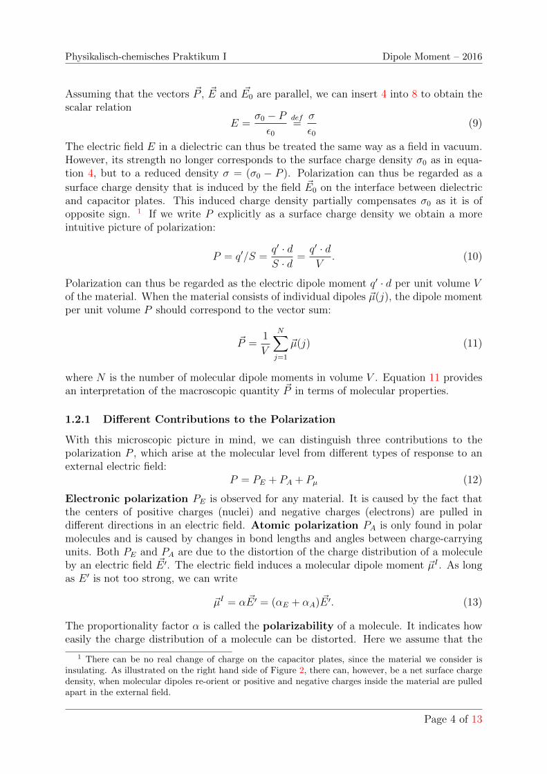
1.2 Relative Permittivity, Polarization, and Polarizability

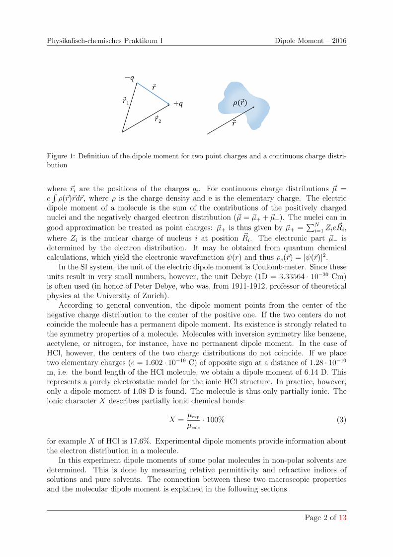
Consider the electric field between two charged plates of a capacitor (in vacuum). If thedistance between the two plates is much smaller than the surface of the plates, the fieldis approximately homogeneous except in the border regions (Figure 2). The electric fieldstrength E0 is given by

E0 =q

Sε0= σ0/ε0 (4)

where σ0 = q/S denotes the surface charge density of one capacitor plate (S = surface area,q = charge on one plate) and ε0 is the vacuum permittivity (ε0 = 8.85419·10−12J−1C2m−1).The voltage U0 between the two plates is proportional to the charge q:

- + - + - +

- + - + - +

- + - + - +

- + - + - +

- + - + - +

- + - + - +

- + - + - +

- + - + - +

- + - + - +

−�+�

+

+

+

+

+

+

+

+

+

+

+

+

-

-

-

-

-

-

-

-

-

-

-

-

�

�

−�+�

+

+

+

+

+

+

+

+

+

+

+

+

-

-

-

-

-

-

-

-

-

-

-

-

�0

�

U0 U

Figure 2: Electric field inside a capacitor with charge q on the capacitor plates and plate spacingd. Left: in vacuum. Right: filled with a dielectric. Polarized and oriented molecules are shownschematically.

q = C0 · U0 (5)

The proportionality factor C0 is called capacitance. Capacitance and field field strengthE0 inside the capacitor are related via:

C0 = q/U0 = q/(E0 · d). (6)

When the capacitor is filled with (non-conducting) matter and charge q and plate sep-aration d are kept constant, the capacitance increases and the voltage is reduced (righthand side of Fig. 2). As a result, the field between the capacitor plates is smaller than invacuum:

C = εC0, U = U0/ε⇒ E = E0/ε (7)

The constant ε > 1 is called relative permittivity of the material (also called dielectric).

It is useful to introduce a quantity called polarization ~P of a dielectric in a field ~E0,defined by:

~P = ε0( ~E0 − ~E) = ε0(ε− 1) ~E (8)

Page 3 of 13

Physikalisch-chemisches Praktikum I Dipole Moment – 2016

Assuming that the vectors ~P , ~E and ~E0 are parallel, we can insert 4 into 8 to obtain thescalar relation

E =σ0 − Pε0

def=

σ

ε0(9)

The electric field E in a dielectric can thus be treated the same way as a field in vacuum.However, its strength no longer corresponds to the surface charge density σ0 as in equa-tion 4, but to a reduced density σ = (σ0 − P ). Polarization can thus be regarded as a

surface charge density that is induced by the field ~E0 on the interface between dielectricand capacitor plates. This induced charge density partially compensates σ0 as it is ofopposite sign. 1 If we write P explicitly as a surface charge density we obtain a moreintuitive picture of polarization:

P = q′/S =q′ · dS · d

=q′ · dV

. (10)

Polarization can thus be regarded as the electric dipole moment q′ · d per unit volume Vof the material. When the material consists of individual dipoles ~µ(j), the dipole momentper unit volume P should correspond to the vector sum:

~P =1

V

N∑j=1

~µ(j) (11)

where N is the number of molecular dipole moments in volume V . Equation 11 providesan interpretation of the macroscopic quantity ~P in terms of molecular properties.

1.2.1 Different Contributions to the Polarization

With this microscopic picture in mind, we can distinguish three contributions to thepolarization P , which arise at the molecular level from different types of response to anexternal electric field:

P = PE + PA + Pµ (12)

Electronic polarization PE is observed for any material. It is caused by the fact thatthe centers of positive charges (nuclei) and negative charges (electrons) are pulled indifferent directions in an electric field. Atomic polarization PA is only found in polarmolecules and is caused by changes in bond lengths and angles between charge-carryingunits. Both PE and PA are due to the distortion of the charge distribution of a moleculeby an electric field ~E ′. The electric field induces a molecular dipole moment ~µI . As longas E ′ is not too strong, we can write

~µI = α ~E ′ = (αE + αA) ~E ′. (13)

The proportionality factor α is called the polarizability of a molecule. It indicates howeasily the charge distribution of a molecule can be distorted. Here we assume that the

1 There can be no real change of charge on the capacitor plates, since the material we consider isinsulating. As illustrated on the right hand side of Figure 2, there can, however, be a net surface chargedensity, when molecular dipoles re-orient or positive and negative charges inside the material are pulledapart in the external field.

Page 4 of 13

Physikalisch-chemisches Praktikum I Dipole Moment – 2016

induced dipole moment ~µI is always oriented in the direction of ~E ′, i.e. that α is a scalar.If the molecules have a permanent dipole moment ~µ0, the total dipole moment in andexternal field is:

~µ = ~µ0 + ~µI (14)

Orientation polarization Pµ is only observed when the molecules have a permanentdipole moment ~µ0. It is caused by a partial alignment of the molecular dipole moments inan electricl field. In contrast to PE and PA, Pµ varies strongly with temperature becausethermal motion opposes the full alignment of the molecular dipoles.

The reason why it is not quite so straightforward to turn equation 11 into a relationbetween measurable quantities, such as ε and the molecular polarizability α and perma-nent dipole moment µ0 is the fact that in dense media the local field ~E ′, which entersin equation 13 or determines the alignment of polar molecules, is not equal (not even on

average) to the macroscopic field ~E of equation 8.

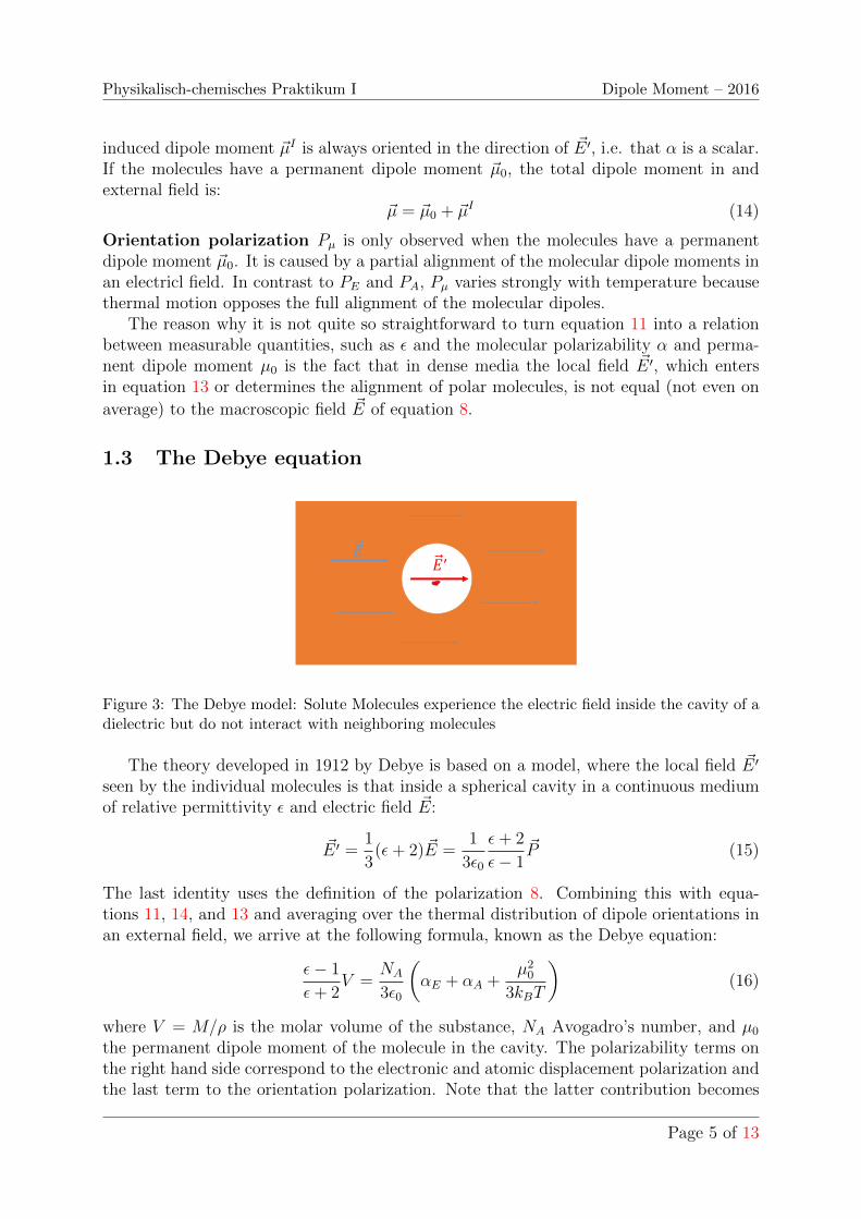
1.3 The Debye equation

�

�’

Figure 3: The Debye model: Solute Molecules experience the electric field inside the cavity of adielectric but do not interact with neighboring molecules

The theory developed in 1912 by Debye is based on a model, where the local field ~E ′

seen by the individual molecules is that inside a spherical cavity in a continuous mediumof relative permittivity ε and electric field ~E:

~E ′ =1

3(ε+ 2) ~E =

1

3ε0

ε+ 2

ε− 1~P (15)

The last identity uses the definition of the polarization 8. Combining this with equa-tions 11, 14, and 13 and averaging over the thermal distribution of dipole orientations inan external field, we arrive at the following formula, known as the Debye equation:

ε− 1

ε+ 2V =

NA

3ε0

(αE + αA +

µ20

3kBT

)(16)

where V = M/ρ is the molar volume of the substance, NA Avogadro’s number, and µ0

the permanent dipole moment of the molecule in the cavity. The polarizability terms onthe right hand side correspond to the electronic and atomic displacement polarization andthe last term to the orientation polarization. Note that the latter contribution becomes

Page 5 of 13

Physikalisch-chemisches Praktikum I Dipole Moment – 2016

smaller with rising temperature, a consequence of thermal motion. The Debye modelneglects polar interactions of dipoles with their surroundings. It is therefore valid only forpolar gases at low pressure or for dilute solutions of polar molecules in non-polar solvents.In the latter case the Debye equation can be re-written:

ε− 1

ε+ 2[V1 + x(V2 − V1)]−

ε1 − 1

ε1 + 2V1(1− x) = x

NA

3ε0

(αE + αA +

µ20

3kBT

)(17)

where x is the mole fraction of the solute, and V1 and V2 are the partial molar volumesof solvent and solute. The relative permittivity ε is that of solvent with solute, while thesolvent alone has a relative permittivity ε1. Quantities on the right hand side only referto solute properties. With the help of this equation, we could in principle determine µ0

of the solute molecules by measuring relative permittivities at different temperatures. Inthis practical course, however, we will employ a different method which makes use of thefact that ε is actually not a constant but is strongly frequency dependent.

1.4 Dispersion

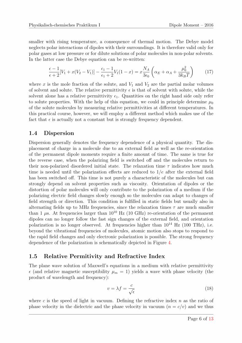
Dispersion generally denotes the frequency dependence of a physical quantity. The dis-placement of charge in a molecule due to an external field as well as the re-orientationof the permanent dipole moments require a finite amount of time. The same is true forthe reverse case, when the polarizing field is switched off and the molecules return totheir non-polarized disordered initial state. The relaxation time τ indicates how muchtime is needed until the polarization effects are reduced to 1/e after the external fieldhas been switched off. This time is not purely a characteristic of the molecules but canstrongly depend on solvent properties such as viscosity. Orientation of dipoles or thedistortion of polar molecules will only contribute to the polarization of a medium if thepolarizing electric field changes slowly enough so the molecules can adapt to changes offield strength or direction. This condition is fulfilled in static fields but usually also inalternating fields up to MHz frequencies, since the relaxation times τ are much smallerthan 1 µs. At frequencies larger than 1010 Hz (10 GHz) re-orientation of the permanentdipoles can no longer follow the fast sign changes of the external field, and orientationpolarization is no longer observed. At frequencies higher than 1014 Hz (100 THz), i.e.beyond the vibrational frequencies of molecules, atomic motion also stops to respond tothe rapid field changes and only electronic polarization is possible. The strong frequencydependence of the polarization is schematically depicted in Figure 4.

1.5 Relative Permitivity and Refractive Index

The plane wave solution of Maxwell’s equations in a medium with relative permittivityε (and relative magnetic susceptibility µm = 1) yields a wave with phase velocity (theproduct of wavelength and frequency):

v = λf =c√ε

(18)

where c is the speed of light in vacuum. Defining the refractive index n as the ratio ofphase velocity in the dielectric and the phase velocity in vacuum (n = c/v) and we thus

Page 6 of 13

Physikalisch-chemisches Praktikum I Dipole Moment – 2016

103 106 109 1012 1015

Frequency (Hz)

Orientation

Atomic

Electronic

Visible

UV

IR

Radio

THz

Figure 4: Schematic representation of the frequency dependence of polarization.

haven2 = ε (19)

i.e. the relative permittivity corresponds to the square of the refractive index n. Itsmagnitude and frequency dependence are a measure for the electronic polarization andits relaxation time. You are probably much more familiar with the refractive index than

�

�

λ1 =�

�1�n1

n2

λ2 =�

�2�

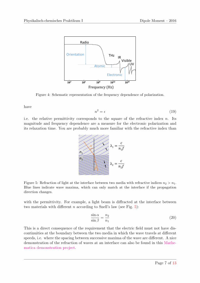
Figure 5: Refraction of light at the interface between two media with refractive indices n2 > n1.Blue lines indicate wave maxima, which can only match at the interface if the propagationdirection changes.

with the permittivity. For example, a light beam is diffracted at the interface betweentwo materials with different n according to Snell’s law (see Fig. 5):

sinα

sin β=n2

n1

(20)

This is a direct consequence of the requirement that the electric field must not have dis-continuities at the boundary between the two media in which the wave travels at differentspeeds, i.e. where the spacing between successive maxima of the wave are different. A nicedemonstration of the refraction of waves at an interface can also be found in this Mathe-matica demonstration project.

Page 7 of 13

Physikalisch-chemisches Praktikum I Dipole Moment – 2016

Here we will use this effect to determine ε at high (optical) frequencies with a re-fractometer. In the region of visible light (4 − 8 · 1014 Hz) we can neglect the atomicpolarizability αA and the static dipole term and replace ε by n2 in equation 17 to obtain:

n2 − 1

n2 + 2[V1 + x(V2 − V1)]−

n21 − 1

n21 + 2

V1(1− x) = xNA

3ε0αE (21)

1.6 The Guggenheim Method

In a paper which appeared in 1949,[1] E. A. Guggenheim combined equations 17 and 21,which essentially eliminates the electronic polarizability αE. He proposed to measure andplot ε and n2 as a function of the solute concentration, yielding the slopes bε and bn2 .Under the assumption that the atomic polarizability αA of a molecule is proportional toits molar volume, he could show that the difference bε − bn2 is equal to

(ε1 + 2)(n21 + 2)

3

NA

3ε0

µ2

3kBT(22)

The corresponding (approximate) formula for the dipole moment of a polar molecules innon-polar solvents is thus:

µ20 =

27kBT

NA

ε01

(ε1 + 2)(n21 + 2)

(bε − bn2) (23)

You will use the Guggenheim method and analyze your experimental data with thisequation. The slopes b can be obtained by plotting ε and n2 against the weight fractionw2 = m2/(m1 + m2). You then need to divide them by ρ1/M2, the ratio of the densityof the pure solvent and the molar mass of the solute. The density (ρ1), the relativepermittivity (ε1) and the refractive index (n1) of the pure solvent must be determinedindependently, or taken from literature.

2 Experiment

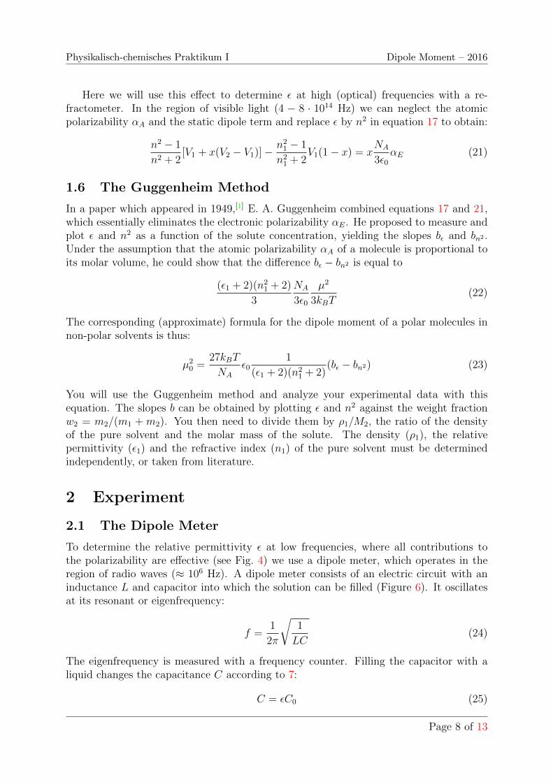
2.1 The Dipole Meter

To determine the relative permittivity ε at low frequencies, where all contributions tothe polarizability are effective (see Fig. 4) we use a dipole meter, which operates in theregion of radio waves (≈ 106 Hz). A dipole meter consists of an electric circuit with aninductance L and capacitor into which the solution can be filled (Figure 6). It oscillatesat its resonant or eigenfrequency:

f =1

2π

√1

LC(24)

The eigenfrequency is measured with a frequency counter. Filling the capacitor with aliquid changes the capacitance C according to 7:

C = εC0 (25)

Page 8 of 13

Physikalisch-chemisches Praktikum I Dipole Moment – 2016

L

C

+V

L’

R

180° Phase shift

L

C

+V

R

(b)(a)AB

switch at A

(charging)

switch at B

(discharging)

∆� =1

�

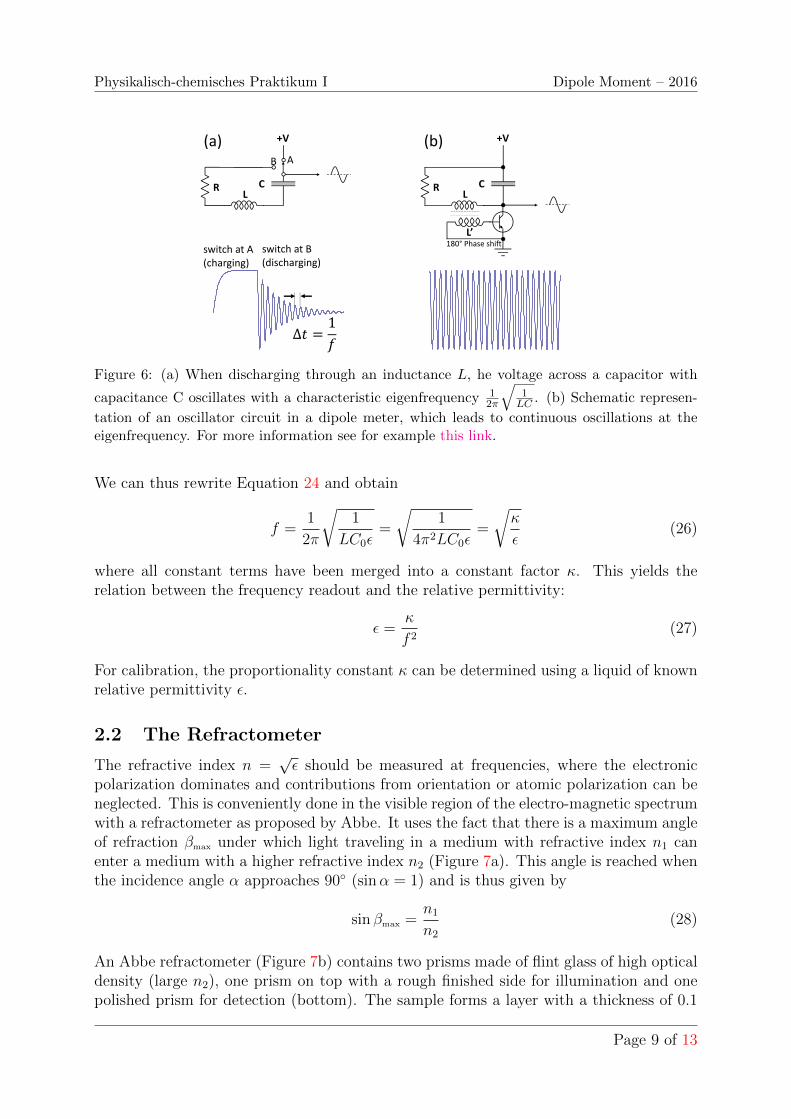
Figure 6: (a) When discharging through an inductance L, he voltage across a capacitor with

capacitance C oscillates with a characteristic eigenfrequency 12π

√1LC . (b) Schematic represen-

tation of an oscillator circuit in a dipole meter, which leads to continuous oscillations at theeigenfrequency. For more information see for example this link.

We can thus rewrite Equation 24 and obtain

f =1

2π

√1

LC0ε=

√1

4π2LC0ε=

√κ

ε(26)

where all constant terms have been merged into a constant factor κ. This yields therelation between the frequency readout and the relative permittivity:

ε =κ

f 2(27)

For calibration, the proportionality constant κ can be determined using a liquid of knownrelative permittivity ε.

2.2 The Refractometer

The refractive index n =√ε should be measured at frequencies, where the electronic

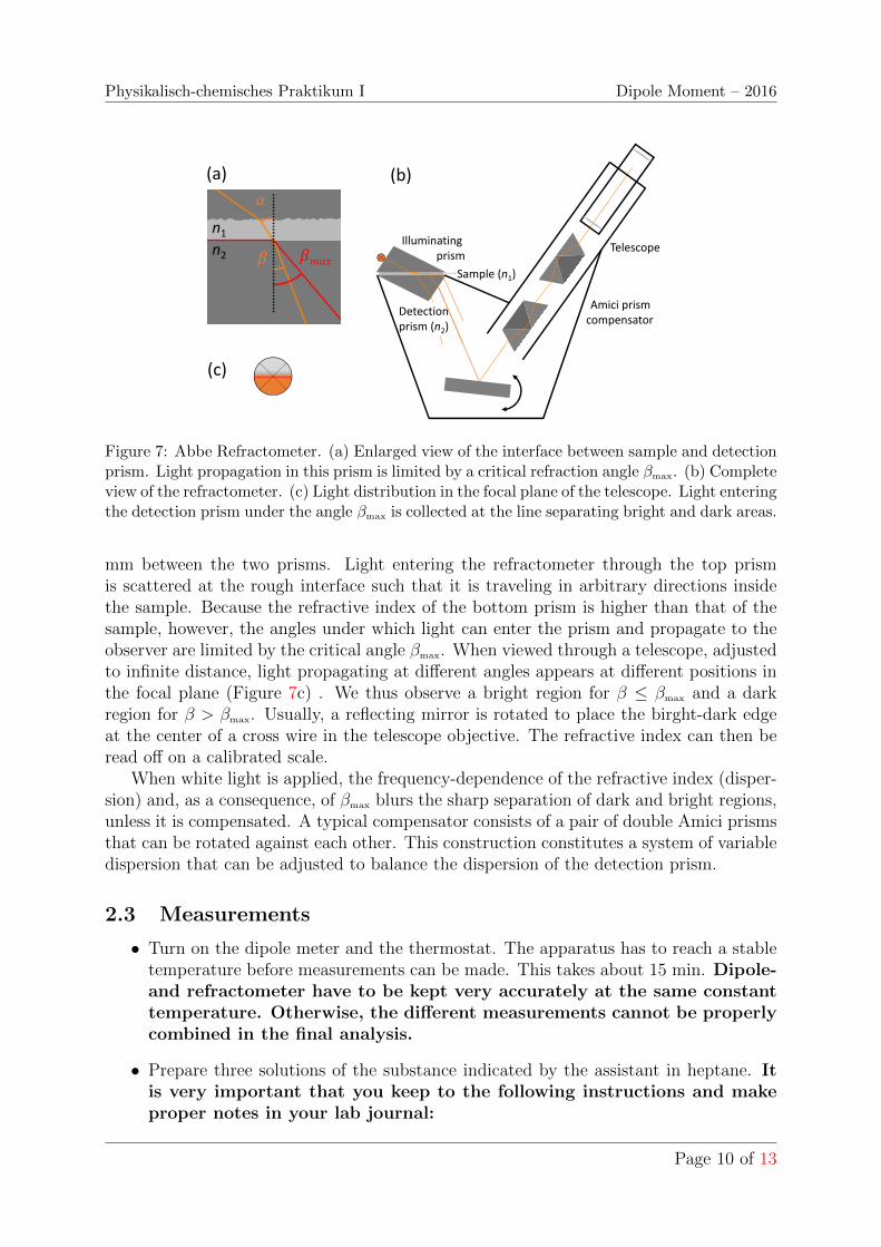
polarization dominates and contributions from orientation or atomic polarization can beneglected. This is conveniently done in the visible region of the electro-magnetic spectrumwith a refractometer as proposed by Abbe. It uses the fact that there is a maximum angleof refraction βmax under which light traveling in a medium with refractive index n1 canenter a medium with a higher refractive index n2 (Figure 7a). This angle is reached whenthe incidence angle α approaches 90◦ (sinα = 1) and is thus given by

sin βmax =n1

n2

(28)

An Abbe refractometer (Figure 7b) contains two prisms made of flint glass of high opticaldensity (large n2), one prism on top with a rough finished side for illumination and onepolished prism for detection (bottom). The sample forms a layer with a thickness of 0.1

Page 9 of 13

Physikalisch-chemisches Praktikum I Dipole Moment – 2016

Sample (n1)

Illuminating

prism

Detection

prism (n2)

Amici prism

compensator

Telescope

(b)

�

�

n1

n2 ����

(a)

(c)

Figure 7: Abbe Refractometer. (a) Enlarged view of the interface between sample and detectionprism. Light propagation in this prism is limited by a critical refraction angle βmax. (b) Completeview of the refractometer. (c) Light distribution in the focal plane of the telescope. Light enteringthe detection prism under the angle βmax is collected at the line separating bright and dark areas.

mm between the two prisms. Light entering the refractometer through the top prismis scattered at the rough interface such that it is traveling in arbitrary directions insidethe sample. Because the refractive index of the bottom prism is higher than that of thesample, however, the angles under which light can enter the prism and propagate to theobserver are limited by the critical angle βmax. When viewed through a telescope, adjustedto infinite distance, light propagating at different angles appears at different positions inthe focal plane (Figure 7c) . We thus observe a bright region for β ≤ βmax and a darkregion for β > βmax. Usually, a reflecting mirror is rotated to place the birght-dark edgeat the center of a cross wire in the telescope objective. The refractive index can then beread off on a calibrated scale.

When white light is applied, the frequency-dependence of the refractive index (disper-sion) and, as a consequence, of βmax blurs the sharp separation of dark and bright regions,unless it is compensated. A typical compensator consists of a pair of double Amici prismsthat can be rotated against each other. This construction constitutes a system of variabledispersion that can be adjusted to balance the dispersion of the detection prism.

2.3 Measurements

• Turn on the dipole meter and the thermostat. The apparatus has to reach a stabletemperature before measurements can be made. This takes about 15 min. Dipole-and refractometer have to be kept very accurately at the same constanttemperature. Otherwise, the different measurements cannot be properlycombined in the final analysis.

• Prepare three solutions of the substance indicated by the assistant in heptane. Itis very important that you keep to the following instructions and makeproper notes in your lab journal:

Page 10 of 13

Physikalisch-chemisches Praktikum I Dipole Moment – 2016

In a 100 mL graduated flask weigh about 100 mL of heptane. Then, using a syringe,add as much sample as you need to obtain a weight fraction of about 3%. 15 mL ofthis solution is put into a second flask (weighed exactly!). The remaining 85 mL arestored well-closed and can be used by other students or to repeat measurements. Di-lute the 15 mL with solvent to 50 mL and weigh again in order to exactly determinethe weight fraction. It should be below 1%. Apply the same procedure to preparea solution with a weight fraction below 0.3%. Carefully note all weights (paraand netto) in your notebook!. You will calculate your exact weight fractionsfrom the actual, measured weights.

• Use a 20 mL syringe and plastic tube to fill the dipole meter with solution or solvent.Do it carefully and make sure, that no liquid is spilled at the top of the cell. Anyair captured between the capacitor plates would perturb the measurement. Afterfilling in solvent or solution, always wait about 5-10 min until the solvent is inthermal equilibrium with the apparatus. Then read off the eigenfrequency from thefrequency counter.

• As a first measurement, measure the pure solvent, i.e. fill the measuring cell withheptane. Read off the frequency at least three times and take an average. Makesure that the cell is clean and dry before any new solution is filled in so that theconcentrations are not changed. Use a dryer first hot, then cold, until no solventcan be smelled. After each measurement, the cell should be rinsed with solvent andthe solvent measured again to check for drifts.

• In parallel, determine εvis by measuring the refractive indices of solvent and allsolutions with the refractometer. Pipette drops of solvent or solution on the detec-tion prism, then close with the lighting prism. After every measurement, clean theprisms using soft tissue and acetone or ethanol. Take care not to scratch theprisms!

• When you have finished with the first substance, repeat the with the (stock-)solutionsprepared by the other groups.

2.4 Practical Advice

• The indicated concentrations do not have to be exactly those specified, but theyhave to be known exactly.

• Check carefully that pipettes, flasks, etc are clean and dry.

• Use different pipettes for different substances.

• Always close the flasks to avoid change of concentration due to evaporation.

• Keep the solutions after the measurements in case you have to repeat some of them.

• Begin with low concentrations and move to higher ones.

Page 11 of 13

Physikalisch-chemisches Praktikum I Dipole Moment – 2016

• When the concentration is changed, the cell has to be rinsed twice with pure solventand dried with the dryer until you cannot smell any solvent.

• Monitor the temperature carefully during the whole experiment. Wait approxi-mately ten minutes after every change of sample such that thermal equilibrium canbe reached.

• Repeat every measurement three times and average the results.

3 Data Analysis

• Use the measurement of the pure solvent with known relative permittivity εHeptane =1.924− 0.00140(T [◦C]− 20) to calculate the calibration constant κ in equation 27.Also determine the experimental uncertainty for κ.

• For each substance, determine the relative permitivitiy of your different solutionsfrom the measured eigenfrequencies (mean values and uncertainties) as well as thecorresponding weight fractions. Plot ε against weight fraction and calculate theslope by linear regression. Specify units and experimental error for the slopes bε.

• Repeat this analysis for the refractive index measurements to obtain the slopes bn2 .

• Use the Guggenheim equation 23 to calculate the static dipole moment µ0 of thesolute molecule. Use error propagation to establish the experimental uncertainty.The density ρ1 of the solvent is given in Table 1 and the molar weight of the dissolvedsubstance M2 should be known.

• Compare your experimental values for the dipole moments of chloro-cyclohexane,dichloromethane, trichloro-methane (chloroform) and monochloro-benzene to refer-ence values from the literature. What does the difference between chloro-cyclohexaneand monochloro-benzene indicate about their charge distributions.

• Use the measured dipole moment of chloro-cyclohexane (µ1) to estimate the ioniccharacter of the C-Cl bond:

X =µ1

d · e(29)

(d = bond length C-Cl, e = elementary charge).

[1–5]

References

[1] E. A. Guggenheim, A proposed simplification in the procedure for computing electricdipole moments, Trans. Faraday Soc. 1949, 45, 714–720 [link].

[2] G. Wedler, H.-J. Freund, Lehrbuch der Physikalischen Chemie, 6th ed., Wiley-VCH,Weinheim, 2012 [link].

Page 12 of 13

Physikalisch-chemisches Praktikum I Dipole Moment – 2016

[3] P. W. Atkins, J. D. Paula, Physikalische Chemie, 5th ed., Wiley - VCH, Weinheim,2013 [link].

[4] C. J. F. Bottcher, P. Bordewijk, Theory of Electric Polarization, vol. II, ElsevierScience, Amsterdam, 1978.

[5] H. B. Thompson, The determination of dipole moments in solution, J. Chem. Educ.1966, 43, 66–73 [link].

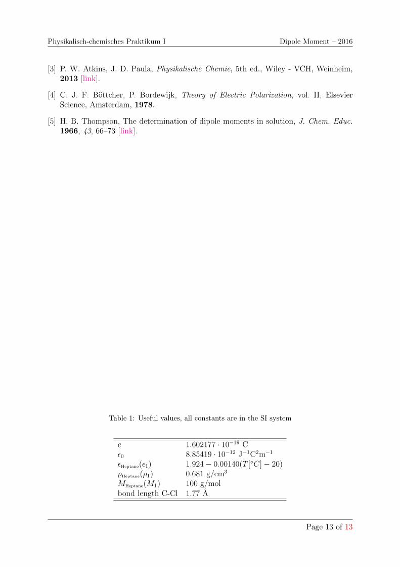
Table 1: Useful values, all constants are in the SI system

e 1.602177 · 10−19 Cε0 8.85419 · 10−12 J−1C2m−1

εHeptane(ε1) 1.924− 0.00140(T [◦C]− 20)ρHeptane(ρ1) 0.681 g/cm3

MHeptane(M1) 100 g/molbond length C-Cl 1.77 A

Page 13 of 13