Dipole tilt effects on the magnetosphere ionosphere …tamas/TIGpapers/2010/2010_Watanabe.pdf · Dipole tilt effects on the magnetosphere‐ionosphere convection system during interplanetary

Dipole tilt effects on the magnetosphere‐ionosphereconvection system during interplanetary magnetic fieldBY‐dominated periods: MHD modeling

Masakazu Watanabe,1 Konstantin Kabin,2 George J. Sofko,3 Robert Rankin,2

Tamas I. Gombosi,4 and Aaron J. Ridley4

Received 17 September 2009; revised 8 December 2009; accepted 14 January 2010; published 21 July 2010.

[1] Using numerical magnetohydrodynamic simulations, we examine the dipole tilteffects on the magnetosphere‐ionosphere convection system when the interplanetarymagnetic field is oblique northward (BY = 4 nT and BZ = 2 nT). In particular, we clarifythe relationship between viscous‐driven convection and reconnection‐driven convection.The azimuthal locations of the two viscous cell centers in the equatorial plane rotateeastward (westward) when the dipole tilt increases as the Northern Hemisphere turnstoward (away from) the Sun. This rotation is associated with nearly the same amountof eastward (westward) rotation of the equatorial crossing point of the dayside separator.The reason for this association is that the viscous cell is spatially confined within theDungey‐type merging cell whose position is controlled by the separator location. Theionospheric convection is basically a round/crescent cell pattern, but the round cellin the winter hemisphere is significantly deformed. Between its central lobe cell portionand its outer Dungey‐type merging cell portion, the round cell streamlines are deformedowing to the combined effects of the viscous cell and the hybrid merging cell, the latterof which is driven by both Dungey‐type reconnection and lobe‐closed reconnection.

Citation: Watanabe, M., K. Kabin, G. J. Sofko, R. Rankin, T. I. Gombosi, and A. J. Ridley (2010), Dipole tilt effects onthe magnetosphere‐ionosphere convection system during interplanetary magnetic field BY‐dominated periods: MHD modeling,J. Geophys. Res., 115, A07218, doi:10.1029/2009JA014910.

1. Introduction

[2] Knowledge of plasma convection is fundamental tothe understanding of the magnetosphere‐ionosphere system[Tanaka, 2007]. On a global scale, the plasma velocity andthe magnetic field are the basic parameters that describe theplasma dynamics [Parker, 1996; Vasyliūnas, 2001, 2005a,2005b]. The concept of convection in the magnetosphere‐ionosphere system started with two pioneering works, bothof which, by a curious coincidence, were published in 1961.Dungey [1961] suggested that for due southward inter-planetary magnetic field (IMF), IMF to closed reconnectionon the dayside and north lobe (NL) to south lobe (SL)reconnection on the nightside drive a plasma circulationmode which appears as two‐cell convection in the iono-sphere (the so‐called Dungey cycle). Axford and Hines

[1961] suggested that the viscous‐like interaction betweenthe solar wind and the magnetospheric plasma in the low‐latitude boundary layer excites morningside and afternoon-side vortices in the closed field line region. A decade later,Russell [1972] proposed that IMF‐NL reconnection or IMF‐SL reconnection produces plasma circulation that is con-fined to the open field line region. These three circulationmodes form the classic framework of steady state convectionin the magnetosphere‐ionosphere system [Reiff and Burch,1985]. In the ionosphere, the convection cells resultingfrom the three circulation modes are called the merging cell(which crosses the polar cap boundary twice in one cycle),the viscous cell (which circulates outside the polar cap), andthe lobe cell (which circulates inside the polar cap). Here,the polar cap is the open field line region in the ionosphere,and we call its equatorward edge (i.e., the open‐closed fieldline boundary) the polar cap boundary.[3] For reconnection‐driven convection, there have been

significant advances since the Reiff and Burch [1985] paper.For due northward IMF and significant dipole tilt, Crooker[1992] suggested a plasma circulation mode which maybe called the “reverse” Dungey cycle. Analogous to the“normal” Dungey cycle, the reverse Dungey cycle proceedsfrom IMF‐closed reconnection at high latitudes in onehemisphere followed by NL‐SL reconnection at high lati-tudes in the opposite hemisphere. As a result, a pair of

1Department of Earth and Planetary Sciences, Graduate School ofSciences, Kyushu University, Fukuoka, Japan.

2Department of Physics, University of Alberta, Edmonton, Alberta,Canada.

3Department of Physics and Engineering Physics, University ofSaskatchewan, Saskatoon, Saskatchewan, Canada.

4Department of Atmospheric, Oceanic, and Space Sciences, Universityof Michigan, Ann Arbor, Michigan, USA.

Copyright 2010 by the American Geophysical Union.0148‐0227/10/2009JA014910

JOURNAL OF GEOPHYSICAL RESEARCH, VOL. 115, A07218, doi:10.1029/2009JA014910, 2010

A07218 1 of 18

reverse merging cells whose circulation directions areopposite to those of the normal Dungey cycle appears in theionosphere in both hemispheres. Later, Tanaka [1999], onthe basis of magnetohydrodynamic (MHD) simulation,suggested a new type of reconnection which occurs betweenlobe field lines and closed field lines. Following this sug-gestion, some new plasma circulation modes were found inassociation with lobe‐closed reconnection. The circulationmode is parameterized by the IMF clock angle *c ≡ Arg(Bz +iBy), where Arg(z) is the function that returns the argumentof a complex number z in the interval −180° < Arg(z) ≤180°. When the IMF is nearly due northward (∣*c∣ ] 30°),lobe‐closed reconnection and IMF‐lobe reconnection formthe “interchange cycle” which produces in the ionosphere a“reciprocal cell” in one hemisphere and an “interchange‐type merging cell” in the other hemisphere [Watanabe et al.,2005; Watanabe and Sofko, 2009a, 2009b]. The reciprocalcell circulates exclusively in the closed field line region, butits circulation direction is opposite to that of the viscous cell.When the IMF BY component is dominant (120° ^ ∣*c∣ ^30°), lobe‐closed reconnection and Dungey‐type reconnec-tion form the “hybrid cycle” which produces in the iono-sphere a variety of “hybrid merging cells” in bothhemispheres [Watanabe et al., 2004, 2007; Watanabe andSofko, 2008].[4] When the IMF BY component is dominant (120° ^

∣*c∣ ^ 30°), ionospheric convection exhibits a distorted two‐cell pattern with its dawn‐dusk and interhemisphericasymmetries regulated by the IMF BY polarity. For IMF BY >0 (BY < 0), in the northern ionosphere, the dawnside (dusk-side) cell is crescent‐shaped, while the duskside (dawnside)cell is relatively round and extends to the dawnside (duskside)ionosphere beyond the noon meridian; the pattern in thesouthern ionosphere is basically a mirror image of thenorthern ionosphere with respect to the noon‐midnightmeridian [e.g., Burch et al., 1985; Lu et al., 1994]. In thispaper, we use the terms “round cell” and “crescent cell” todescribe the IMF BY‐regulated convection cells. In the classicframework of Reiff and Burch [1985], the round cell con-sists of a merging cell and a lobe cell, while the crescentcell consists of a merging cell and a viscous cell. In the

reconnection‐based modern view of Watanabe et al. [2007]and Watanabe and Sofko [2008, 2009a], the round cell con-sists of a lobe cell, a Dungey‐type merging cell, and a hybridmerging cell, whereas the crescent cell is a pure Dungey‐typemerging cell. Note that in both the classic and modern pic-tures, the round cell does not include a viscous cell.[5] In the modern picture, the round cell is a consequence

of four types of reconnection, namely, IMF‐closed, IMF‐lobe, lobe‐lobe, and lobe‐closed. When the X lines of thefour types of reconnection are projected to the ionosphere inthe same hemisphere as the null point, they are anchored tothe foot point of the “stemline” [Siscoe et al., 2001b] whichconnects the magnetic null and the ionosphere (we call thispoint the topological cusp). Because of this spatial constrainton the projected X lines, the convection pattern in thishemisphere is a structurally stable round cell. Observationsalso support the stability of the round cell, because theround cell pattern is almost always observed during IMFBY‐dominated periods. However, the authors of this paper,who have been analyzing Super Dual Auroral Radar Net-work (SuperDARN) data, have recently found severalexceptional examples as sketched in Figure 1. This is aconvection pattern observed in the Northern Hemisphere forIMF BY > BZ > 0. Although it still holds the basic round/crescent cell structure, in this case the round cell on theduskside transforms into double cells. Since these exampleswere found exclusively around the December solstice, it wassuspected that the transformation was due to dipole tilteffects. Motivated by this expectation, we investigate in thispaper the dipole tilt effects on the magnetosphere‐ionosphereconvection system by means of numerical MHD simulation.Our aim is to provide a useful guide for interpreting obser-vational data. A detailed comparison between observationsand simulations will be submitted in future studies.

2. Outlook

[6] In magnetospheric studies, two coordinate systems areusually used: the Geocentric Solar Magnetospheric (GSM)coordinate system and the Solar Magnetic (SM) coordinatesystem [e.g., Kivelson and Russell, 1995, Appendix 3]. TheEarth’s dipole axis is parallel to the SM Z axis. When thedipole is tilted, the GSM Z axis and the SM Z axis are notparallel. We define the dipole tilt angle D as the signedangle between the GSM Z axis and the SM Z axis andpositive for boreal summer. The value of D approximatelyranges from −35° around 0500 UT on the December solsticeto +35° around 1700 UT on the June solstice. In this paper,we use the GSM coordinates exclusively for presenting thesimulation results.[7] We examine the effect of dipole tilt on the

magnetosphere‐ionosphere convection system during IMFBY‐dominated periods by using the BATS‐R‐US MHDsimulation code [Powell et al., 1999]. For this purpose, weperformed three simulation runs for which the IMF and solarwind conditions remained the same but the dipole tilt anglechanged as follows: (1) D = 0°, (2) D = −20°, and (3) D =−35°. For all three runs, the IMF parameters were set as BX =0 nT, BY = 4 nT, and BZ = 2 nT (*c = 63°), and the solar windparameters were set as v = 400 km/s (speed), r = 5 amu/cc(mass density), and T = 50,000 K (temperature). In order toexclude ionospheric conductance effects, we assumed uni-

Figure 1. An uncommon convection pattern in the North-ern Hemisphere seen near the December solstice for IMFBY > BZ > 0.

WATANABE ET AL.: DIPOLE TILT EFFECT ON CONVECTION SYSTEM A07218A07218

2 of 18

Figure 2


3 of 18

form ionospheric conductances, namely SP = 1 S (Pedersenconductance) and SH = 0 S (Hall conductance), for bothhemispheres. The latter condition was deliberately chosen inorder to exclude the dawn‐dusk asymmetry which ariseswhen there is a finite Hall conductance [Ridley et al., 2004].[8] Figure 2 shows ionospheric potentials for the three

simulation runs, with Figures 2a, 2c, and 2e showing theNorthern Hemisphere and Figures 2b, 2d, and 2f showingthe Southern Hemisphere. Potential contours (Figure 2, solidlines) are shown every 3 kV and labeled every 6 kV. Figure 2indicates that, for all the six cases, the potential contoursexhibit the basic round/crescent cell pattern. Point a (point d)indicates the center of the round (crescent) cell. The largedotted loop encircling the polar region represents the polarcap boundary. Since point a (point d) is located far poleward(equatorward) of the polar cap boundary, the round (crescent)cell includes a substantial lobe (viscous) cell at its center.Point m (point n) on the polar cap boundary is the topo-logical cusp in the Northern (Southern) Hemisphere. Asthe magnitude of the dipole tilt increases, the polar cap inthe summer hemisphere becomes heart‐shaped owing to thepoleward deformation near the topological cusp (Figures 2dand 2f). This polar cap shape is consistent with that for thedue northward IMF case [Crooker, 1992, Figure 3;Watanabeet al., 2005, Figure 2]. Point b (point c) in Figure 2 indicatesthe location of the potential peak on the round‐cell‐side(crescent‐cell‐side) polar cap boundary. The dotted line thatpasses point b (point c) and lies poleward (equatorward)of the polar cap boundary is the potential contour thatdemarcates the boundary between the lobe (viscous) celland the merging cell.[9] We here introduce two new terms for the following

discussion. For the BY > 0 case, on the duskside, the round(crescent) cell appears in the Northern (Southern) Hemi-sphere. Conversely, on the dawnside, the round (crescent)cell appears in the Southern (Northern) Hemisphere. In thispaper, we examine the “conjugate” round and crescent cellson the duskside or dawnside. In order to deal with theduskside and dawnside convection systems synthetically,we use the terms “round cell hemisphere” and “crescent cellhemisphere.” For the BY > 0 case, on the duskside (dawn-side), the round cell hemisphere means the Northern(Southern) Hemisphere, whereas the crescent cell hemispheremeans the Southern (Northern) Hemisphere.[10] The convection pattern revealed by the simulation

(Figure 2) poses two questions. First, when the dipole istilted significantly, the round cell in the winter hemisphere isnot really round but tadpole‐shaped (Figures 2c and 2e),which is very similar to the pattern in Figure 1, although the

simulated round cell does not split into two as observed.Why does this deformation occur? Second, although thecrescent cell includes a substantial viscous cell, the conju-gate round cell in the opposite hemisphere does not. Viscouscells are considered to be excited in the equatorial region. Insection 3.1, we determine viscous cells in the equatorialplane. Point r (point s) in Figure 2 shows the projection ofthe equatorial viscous cell center to the round (crescent) cellhemisphere. In the crescent cell hemisphere, the viscous cellappears almost intact, naturally embedded in the mergingcell. In contrast, in the round cell hemisphere, the originalviscous cell in the equatorial plane is overall obliterated bythe merging cell. Where does this interhemispheric differ-ence come from? Actually the round cell deformation andthe interhemispheric viscous cell asymmetry are closelyrelated. The goal of this paper is to elucidate the relationbetween the viscous cell and the round cell and clarify itsdipole tilt dependence. For this purpose, in section 3, wefirst explore the magnetospheric convection, both viscous‐driven and reconnection‐driven. To understand these pro-cesses, one needs to know the geometry and topology of themagnetosphere. We then in section 4 return to Figure 2 anddiscuss the dipole tilt effect on the ionospheric convection.We consider how the viscous‐driven convection and thereconnection‐driven convection mutually affect each otherin the ionosphere.

3. Structure of the Magnetosphere: GeometricalRelationship Between the Viscous Circulationand the Dungey Circulation

3.1. Viscous Cells

[11] We first describe the geometry of the viscous cellsgenerated in the equatorial region. In the simulated mag-netosphere‐ionosphere system in this paper, in addition toreconnection‐driven convection, “viscous convection” playsan important role. By the word “viscous convection,” wemean that, when looking downward on the equatorial planefrom the north, there are a clockwise convection cell on thedawnside and a counterclockwise convection cell on theduskside circulating in the closed field line region. Note thatthis identification is purely morphological even though itsname suggests a physical process. The name “viscous”derives from the suggestion by Axford and Hines [1961,Figure 3] that the viscous‐like interaction between the solarwind and the magnetospheric plasma excites two convectioncells in the magnetosphere. In the BATS‐R‐US code,however, there is no physical viscosity in the governingequations. It is known nevertheless that ideal‐MHD simula-

Figure 2. Ionospheric potential contours (solid lines) for (a, b) D = 0°, (c, d) D = −20°, and (e, f) D = −35° in the northernionosphere (Figures 2a, 2c, and 2e) and southern ionosphere (Figures 2b, 2d, and 2f). The polar azimuthal equidistant pro-jection is used. The contours are labeled every 6 kV. The large dotted loop centered on the geomagnetic pole shows theopen‐closed field line boundary (i.e., polar cap boundary). Point m in Figures 2a, 2c, and 2e represents the topological cuspin the Northern Hemisphere (the foot point of stemline s1 in Figure 4), while point n in Figures 2b, 2d, and 2f represents thetopological cusp in the Southern Hemisphere (the foot point of stemline s2 in Figure 4). Point a (point d) represents the center ofthe round cell (crescent cell). Point b (point c) shows the location of the potential peak on the polar cap boundary on the roundcell side (crescent cell side). Point r (point s) represents the ionospheric projection of the equatorial viscous cell center to theround cell (crescent cell) hemisphere. The small dotted loop passing through point b and centered on point a is the demarcationcontour between the lobe cell and the merging cell. The dotted loop passing through point c and centered on point d (only partof it is seen for Figures 2d and 2f) is the demarcation contour between the viscous cell and the merging cell.


4 of 18

tions can reproduce the “viscous cells”morphologically, withthe cells conceivably driven by numerical viscosity. Thissituation is similar to that of reconnection driven by numericalresistivity in ideal‐MHD simulations. However, while weempirically know that reconnection resulting from numericalresistivity in magnetospheric simulations can reproduce themagnetospheric morphology reasonably well, the effects ofnumerical viscosity in this context have not been studiedextensively. Thus the issue of how well our simulation canreproduce the actual viscous cells (if they exist) in the mag-netosphere remains an open problem.[12] Figure 3 shows the three‐dimensional streamlines in

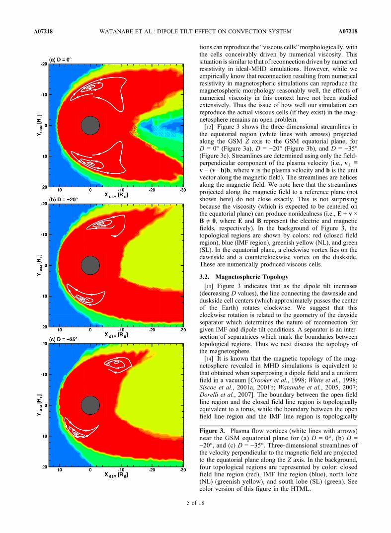
the equatorial region (white lines with arrows) projectedalong the GSM Z axis to the GSM equatorial plane, forD = 0° (Figure 3a), D = −20° (Figure 3b), and D = −35°(Figure 3c). Streamlines are determined using only the field‐perpendicular component of the plasma velocity (i.e., v? ≡v − (v · b)b, where v is the plasma velocity and b is the unitvector along the magnetic field). The streamlines are helicesalong the magnetic field. We note here that the streamlinesprojected along the magnetic field to a reference plane (notshown here) do not close exactly. This is not surprisingbecause the viscosity (which is expected to be centered onthe equatorial plane) can produce nonidealness (i.e., E + v ×B ≠ 0, where E and B represent the electric and magneticfields, respectively). In the background of Figure 3, thetopological regions are shown by colors: red (closed fieldregion), blue (IMF region), greenish yellow (NL), and green(SL). In the equatorial plane, a clockwise vortex lies on thedawnside and a counterclockwise vortex on the duskside.These are numerically produced viscous cells.

3.2. Magnetospheric Topology

[13] Figure 3 indicates that as the dipole tilt increases(decreasing D values), the line connecting the dawnside andduskside cell centers (which approximately passes the centerof the Earth) rotates clockwise. We suggest that thisclockwise rotation is related to the geometry of the daysideseparator which determines the nature of reconnection forgiven IMF and dipole tilt conditions. A separator is an inter-section of separatrices which mark the boundaries betweentopological regions. Thus we next discuss the topology ofthe magnetosphere.[14] It is known that the magnetic topology of the mag-

netosphere revealed in MHD simulations is equivalent tothat obtained when superposing a dipole field and a uniformfield in a vacuum [Crooker et al., 1998; White et al., 1998;Siscoe et al., 2001a, 2001b; Watanabe et al., 2005, 2007;Dorelli et al., 2007]. The boundary between the open fieldline region and the closed field line region is topologicallyequivalent to a torus, while the boundary between the openfield line region and the IMF line region is topologically

Figure 3. Plasma flow vortices (white lines with arrows)near the GSM equatorial plane for (a) D = 0°, (b) D =−20°, and (c) D = −35°. Three‐dimensional streamlines ofthe velocity perpendicular to the magnetic field are projectedto the equatorial plane along the Z axis. In the background,four topological regions are represented by color: closedfield line region (red), IMF line region (blue), north lobe(NL) (greenish yellow), and south lobe (SL) (green). Seecolor version of this figure in the HTML.


5 of 18

equivalent to a cylinder. The torus is touching the cylinderalong a circle which consists of two magnetic field linescalled separators. There are two magnetic nulls on the sep-arator circle, and the separators connect the two magneticnulls. Figure 4 shows a simplified schematic of this mag-netospheric topology for northward IMF. Here we followWatanabe et al. [2007, Figure 2] and Watanabe and Sofko[2008, Figure 1] for the notation signifying magnetic nulls(M and N), separatrices (a, b, g, and d), separators (l1 andl2), and singular lines (s1, s2, s3, and s4). Separatrices a andb form a torus, while separatrices g and d form a cylinder.Separators l1 and l2 lie where the torus and the cylindermeet. Field lines on the torus (cylinder) are shown by dotted(solid) lines with arrows. All the field lines on separatrices a

and g converge to null M, except for the two singular fieldlines (s2 on separatrix a and s4 on separatrix g) that con-verge to null N. Similarly, all the field lines on separatricesb and d diverge from null N, except for the two singularlines (s1 on separatrix b and s3 on separatrix d) that divergefrom null M. The singular lines connecting the null points tothe ionosphere (s1 and s2 in Figure 4) are called “stemlines”[Siscoe et al., 2001b].[15] The locations of the magnetic null points and separa-

tors determine the geometry of the magnetosphere and con-sequently the types of reconnection that occur for the givenIMF orientation and the given dipole tilt. For IMF BY > 0, theNorthern Hemisphere magnetic null (M) is on the duskside,while the Southern Hemisphere magnetic null (N) is on the

Figure 4. Separatrix surfaces (topologically equivalent to a torus and a cylinder) for northward IMF.Solid lines with arrows represent the field lines on the cylinder surface, while dotted lines with arrowsrepresent the field lines on the torus surface.


6 of 18

dawnside. If there is no dipole tilt, the dayside separatorpasses through the subsolar point and roughly lies on theplane Z = Y cot*M in GSM coordinates, where *M is the clockangle of null M (*M = Arg(ZM + iYM)). However, when thedipole is tilted, the dayside separator is not in the Z = Y cot*Mplane. Table 1 shows the positions of the null points for thethree simulation runs. In the null search, we did not use asophisticated algorithm such as that proposed by Greene[1992]. The null point locations were determined simply bysearching a magnetic field minimum on the grid points. Thisbrute‐force method is sufficient for the discussion in thispaper. For D = 0°, the two nulls are symmetric about the Xaxis, and they are located roughly in the dawn‐dusk plane(X = 0). The clock angle of null M for D = 0° is *M = 33°.In the vacuum superposition model, *M is given by

*M ¼ arctan" ffiffiffiffiffiffiffiffiffiffiffiffiffiffiffiffi

8þ9 cot2 *cp

&3 cot *c2

#(0° < *c < 180°) [Yeh, 1976].

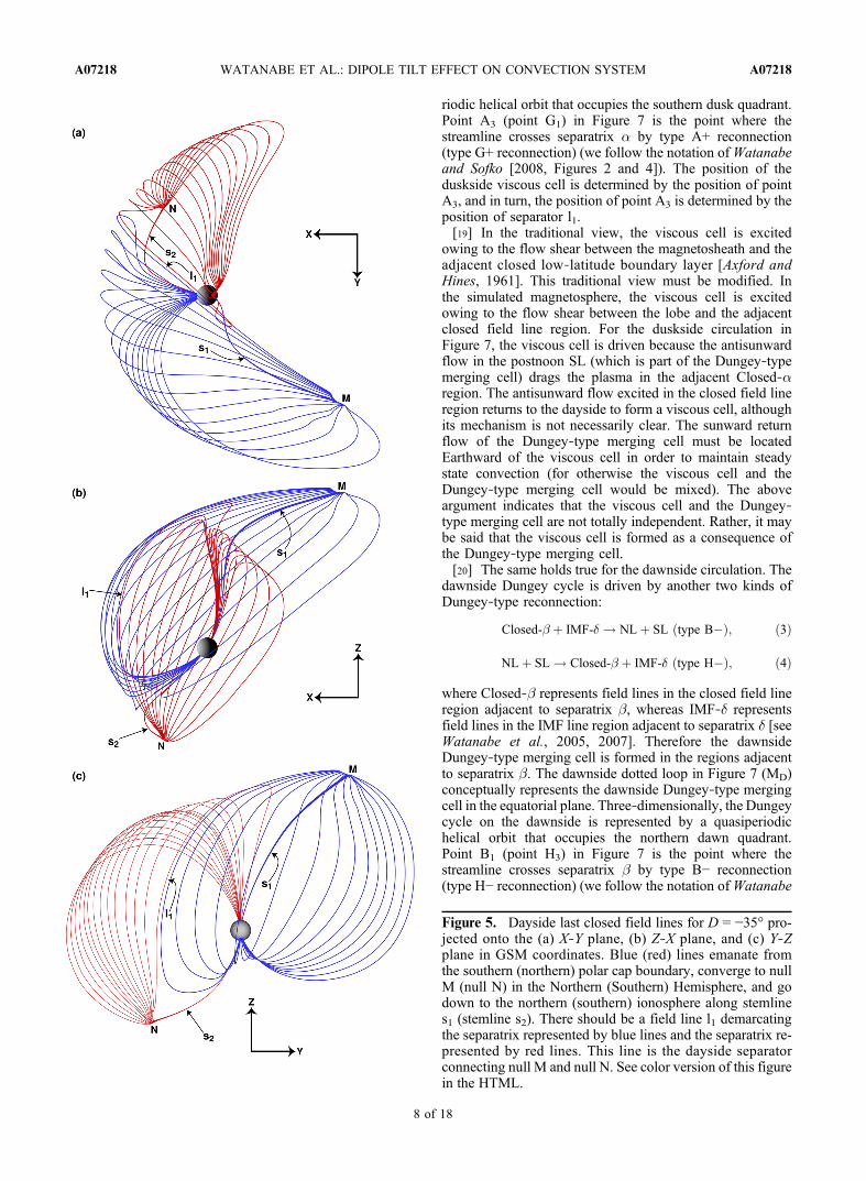
Our simulation result (*M = 33°) shows some deviation fromthe vacuum superposition model (*M = 40°). As the dipoletilt becomes large (with decreasing D), the NorthernHemisphere null (null M) moves away from the Sun, whilethe Southern Hemisphere null (null N) moves toward the Sun.Accordingly the dayside separator does not pass through thesubsolar point.[16] Figure 5 demonstrates the dayside last closed field

lines for D = −35° projected onto the X‐Y plane (Figure 5a),Z‐X plane (Figure 5b), and Y‐Z plane (Figure 5c) in GSMcoordinates. Nightside last closed field lines are not shownas they are very hard to visualize clearly and are notessential for our discussion. Blue (red) lines emanate frominfinitesimally equatorward of the Southern (Northern)Hemisphere polar cap boundary and converge to the vicinityof null M (null N), forming a surface within separatrix a(separatrix b). This surface virtually represents separatrix a(separatrix b). The field line bundle then goes down to thenorthern (southern) ionosphere along stemline s1 (stemline s2).The dayside juncture of separatrices a and b is separator l1,a field line which emanates from null N and convergesto null M. Although the existence of such a field line isobvious in Figure 5, it is difficult to extract separator l1 fromthe simulation data because of numerical errors. In Figure 5,we indicated the expected location of separator l1 in theequatorial region where blue lines representing separatrix aand red lines representing separatrix b come close together.Figure 5 indicates that the route of the dayside separator l1shifts dawnward and northward compared to the route forD =0° which is approximately in the Z = Y cot33° plane. Con-sequently, in the Y‐Z plane in Figure 5c, (blue) separatrix adominates in the area facing the Sun, which means that SLfield lines (which are facing separatrix a) drape over thedayside magnetosphere more than NL field lines (which arefacing separatrix b).

3.3. Relation Between the Viscous Cell and theDungey‐Type Merging Cell

[17] As Figure 5a indicates, the dayside separator for D =−35° crosses the GSM equatorial plane at a point about 43°westward of the subsolar point. (The precise location mustbe determined from Figures 5b and 5c because the equato-rial crossing point of l1 does not correspond to the largestdistance from the Z axis.) The equatorial crossing point ofseparator l1 is correlated with the positions of the two vis-cous cells. In order to investigate this relation, we define theazimuth angle y of a point (X, Y) on the equatorial plane asy ≡ Arg (X + iY). Figure 6 shows the dipole tilt dependenceof the azimuth angle of the duskside viscous cell center, theequatorial crossing point of the dayside separator, and thedawnside viscous cell center. Here, the data points for D ≥ 0were determined assuming that the configurations for D =D0 ≥ 0 are obtained by rotating 180° about the X axis theconfigurations for D = −D0 (although one must reverse thedirection of the magnetic field). This assumption, which wecall the rotational symmetry assumption, will be usedthroughout this paper. Figure 6 indicates that relative to theequatorial crossing point of the dayside separator, the twoviscous cells have an angular separation which ranges from78° to 107° (∼90° on average). Figure 7 schematicallydepicts this geometrical relationship for the D = −35° case(a sketch from Figures 3c and 5a). The equatorial crossingpoint of the dayside separator (l1) is located in the prenoonsector. The two viscous cells appear roughly 90° east andwest of this point.[18] There is a simple interpretation of the geometrical

relationship between the viscous cell positions and theequatorial crossing point of the dayside separator. The vis-cous cell always appears inside the Dungey‐type mergingcell. Thus the location of the viscous cell is constrained bythe location of the Dungey‐type merging cell. In turn, theDungey‐type merging cell is constrained by the geometry ofthe separatrices. For the BY > 0 case we are considering, theduskside Dungey cycle is driven by two kinds of Dungey‐type reconnection:

Closed-(þ IMF-% ! NLþ SL ðtype AþÞ; ð1Þ

NLþ SL! Closed-(þ IMF-% ðtype GþÞ; ð2Þ

where Closed‐a represents field lines in the closed field lineregion adjacent to separatrix a, whereas IMF‐g representsfield lines in the IMF line region adjacent to separatrix g.We also use Closed‐a and IMF‐g to represent the topo-logical regions occupied by those field lines [seeWatanabe etal., 2005, 2007]. The open‐closed flux transport associatedwith the duskside Dungey cycle occurs through separatrix a.Therefore the duskside Dungey‐type merging cell is formedin the regions adjacent to separatrix a. The duskside dottedloop in Figure 7 (MD) represents the duskside Dungey‐typemerging cell in the equatorial plane. Note that MD representsthe conceptual Dungey‐type merging cell projected to theequatorial plane along the field lines. Actually there is nosuch two‐dimensional closed orbit in the equatorial plane.Also the three‐dimensional orbit does not close, as we notedin the viscous cells in Figure 3. The three‐dimensionalDungey cycle on the duskside is represented by a quasipe-

Table 1. Null Point Positions in GSM Coordinates

Northern HemisphereNull M

Southern HemisphereNull N

Dipole Tilt X (RE) Y (RE) Z (RE) X (RE) Y (RE) Z (RE)

D = 0° −1.250 8.250 12.500 −1.250 −8.250 −12.500D = −20° −8.500 10.000 14.750 2.250 −8.000 −10.500D = −35° −12.000 9.750 15.250 4.375 −7.750 −9.125


7 of 18

riodic helical orbit that occupies the southern dusk quadrant.Point A3 (point G1) in Figure 7 is the point where thestreamline crosses separatrix a by type A+ reconnection(type G+ reconnection) (we follow the notation ofWatanabeand Sofko [2008, Figures 2 and 4]). The position of theduskside viscous cell is determined by the position of pointA3, and in turn, the position of point A3 is determined by theposition of separator l1.[19] In the traditional view, the viscous cell is excited

owing to the flow shear between the magnetosheath and theadjacent closed low‐latitude boundary layer [Axford andHines, 1961]. This traditional view must be modified. Inthe simulated magnetosphere, the viscous cell is excitedowing to the flow shear between the lobe and the adjacentclosed field line region. For the duskside circulation inFigure 7, the viscous cell is driven because the antisunwardflow in the postnoon SL (which is part of the Dungey‐typemerging cell) drags the plasma in the adjacent Closed‐aregion. The antisunward flow excited in the closed field lineregion returns to the dayside to form a viscous cell, althoughits mechanism is not necessarily clear. The sunward returnflow of the Dungey‐type merging cell must be locatedEarthward of the viscous cell in order to maintain steadystate convection (for otherwise the viscous cell and theDungey‐type merging cell would be mixed). The aboveargument indicates that the viscous cell and the Dungey‐type merging cell are not totally independent. Rather, it maybe said that the viscous cell is formed as a consequence ofthe Dungey‐type merging cell.[20] The same holds true for the dawnside circulation. The

dawnside Dungey cycle is driven by another two kinds ofDungey‐type reconnection:

Closed-' þ IMF-$ ! NLþ SL ðtype B&Þ; ð3Þ

NLþ SL! Closed-' þ IMF-$ ðtype H&Þ; ð4Þ

where Closed‐b represents field lines in the closed field lineregion adjacent to separatrix b, whereas IMF‐d representsfield lines in the IMF line region adjacent to separatrix d [seeWatanabe et al., 2005, 2007]. Therefore the dawnsideDungey‐type merging cell is formed in the regions adjacentto separatrix b. The dawnside dotted loop in Figure 7 (MD)conceptually represents the dawnside Dungey‐type mergingcell in the equatorial plane. Three‐dimensionally, the Dungeycycle on the dawnside is represented by a quasiperiodichelical orbit that occupies the northern dawn quadrant.Point B1 (point H3) in Figure 7 is the point where thestreamline crosses separatrix b by type B− reconnection(type H− reconnection) (we follow the notation ofWatanabe

Figure 5. Dayside last closed field lines for D = −35° pro-jected onto the (a) X‐Y plane, (b) Z‐X plane, and (c) Y‐Zplane in GSM coordinates. Blue (red) lines emanate fromthe southern (northern) polar cap boundary, converge to nullM (null N) in the Northern (Southern) Hemisphere, and godown to the northern (southern) ionosphere along stemlines1 (stemline s2). There should be a field line l1 demarcatingthe separatrix represented by blue lines and the separatrix re-presented by red lines. This line is the dayside separatorconnecting null M and null N. See color version of this figurein the HTML.


8 of 18

Figure 6. The dipole tilt dependence of the azimuth angles of the vortex centers in the equatorial planeand the equatorial crossing point of the dayside separator, for IMF *c = 63°. The data points for D ≥ 0were determined from the simulation results for D ≤ 0 by assuming the rotational symmetry (see text).

Figure 7. A sketch for the D = −35° case showing the geometrical relationship between the dayside sep-arator (l1) and the equatorial viscous cells (V). Separatrices (a, b, g, and d) divide the entire space into sixtopological regions (IMF‐g, IMF‐d, NL, SL, Closed‐a, and Closed‐b). The dashed line represents thedemarcation between IMF‐g and IMF‐d and between Closed‐a and Closed‐b. The dotted loops (MD)represent the dawnside and duskside Dungey cycles projected to the equatorial plane along the field lines.Note that there are no such two‐dimensional closed orbits in the equatorial plane. Three‐dimensionalDungey cycles are found in the northern dawn quadrant and in the southern dusk quadrant as quasi-periodic helical orbits. Points B1, H3, A3, and G1 represent the points where the Dungey cycle orbitcrosses the separatrix.


9 of 18

and Sofko [2008, Figures 3 and 5]). The position of thedawnside viscous cell is determined by the position of pointB1, and in turn, the position of point B1 is determined by theposition of separator l1.[21] The dashed line in Figure 7 conceptually represents

the demarcation between Closed‐a and Closed‐b andbetween IMF‐g and IMF‐d. For the convection systemduring IMF BY‐dominated periods, the dashed line alsorepresents the demarcation between the dawnside circulationand the duskside circulation. In the steady state convectionsystem, there is no magnetic flux transport across the dashedline. Here the “steady state”means that themagnetic topologyin Figure 4 is conserved at any point of time. Plasma flowacross the dashed line indicates the mixture of dawnside andduskside circulations, which is only possible when the null‐separator structure in Figure 4 breaks down, at least tempo-rally. As the magnitude of the dipole tilt increases, thedemarcation line in the closed field line region rotatesclockwise for D < 0 or counterclockwise for D > 0. Theazimuth angles of Dungey‐type merging cells and theembedded viscous cell also rotate clockwise or counter-clockwise accordingly.

4. Dipole Tilt Effects on the IonosphericConvection Pattern

4.1. Ideal Convection Pattern

[22] To begin with, we discuss the expected ionosphericconvection (or potential) pattern for the ideal case; that is,E +v × B = 0 everywhere except in the portions of the equatorialregion where the viscous cells are generated and the diffu-sion regions on the separatrices where reconnection takesplace. The diffusion region is characterized by a nonvan-ishing parallel (field‐aligned) electric field. However, sincethe simulation code solves the equations of ideal MHD, itis in principle impossible to identify the diffusion regionsin the simulated magnetosphere. Yet we infer that, exceptfor the nightside Dungey‐type reconnection, the diffusionregions are located at high latitudes near the magneticnull points where antiparallel field line geometry tends tooccur. In addition, because the diffusion region has a three‐dimensional extent, the ionospheric projection of the diffu-sion region is a two‐dimensional area. Since we do not knowthe exact extent of the diffusion region or the spatial distri-bution of the parallel electric field, it is very difficult toexamine the ionospheric potentials in this problem setting.However, we can gain insight into this problem by employingthe “current penetration model” of Watanabe et al. [2007],which provides basically the same ionospheric consequencesas the original three‐dimensional diffusion region case. Thename “current penetration model” was introduced by Siscoe[1988] to describe the merging models that allow a normalcomponent of the magnetic field on the separatrix. This classof merging models was first proposed by Alekseyev andBelen’kaya [1983]. In the current penetration model ofWatanabe et al. [2007], the diffusion region is representedby a field line segment on the separatrix (which we call theX line), with a small magnetic field component normal to theseparatrix in the vicinity of the X line. This configuration isconsidered to be the limit when the three‐dimensional diffu-

sion region collapses into a line on the MHD scale. The meritof this model is that the electric field along the X line isdirectly mapped to the ionosphere as a perpendicular (to B)electric field.[23] Figure 8 shows the duskside convection pattern in the

Northern Hemisphere (Figures 8a and 8b) and the SouthernHemisphere (Figure 8c) for IMF BY > 0. The differencebetween Figures 8a and 8b is that while Figure 8a shows asimple superposition of convection cell elements, Figure 8bshows the resultant net convection. The patterns in Figures8a and 8c are basically the same as those described byWatanabe et al. [2007, Figure 9] and Watanabe and Sofko[2008, Figure 6], except for the addition of a viscous cell.In the discussion in section 3.3 of the reconnection‐drivenequatorial convection on the duskside, we only needed toconsider Dungey‐type reconnection (type A+ and type G+).In the ionosphere, however, we also need to consider twokinds of interchange‐type reconnection contributing to theduskside convection system:

IMF-% þ NL! NLþ IMF-% ðtype C&Þ; ð5Þ

SLþ Closed-(! Closed-(þ SL ðtype EþÞ: ð6Þ

The thick solid lines in Figure 8 are projected X lines withsymbols A3, A4, C4, E1, E3, E4, G1, and G4 corresponding tothose ofWatanabe et al. [2007, Figure 7] andWatanabe andSofko [2008, Figures 2 and 4]. The kernel letters (A, C, E,and G) represent the location of the diffusion region. Theduskside portion of G4 in Figures 8a and 8b is drawn with adotted line in order to show that type G+ reconnection is notactive on the duskside flank. Lines A3 and G1 in Figure 8ccorrespond to points A3 and G1 in Figure 7, respectively.That is, the convection cell labeled MD in Figure 8c is theionospheric projection of the duskside Dungey‐type merg-ing cell in Figure 7. The dashed loop (partly overlapped withthe projected X lines) is the polar cap boundary, which is theionospheric cross section of separatrix b (Figures 8a and 8b)or separatrix a (Figure 8c). Point m in Figures 8a and 8b(point n in Figure 8c) is the foot point of stemline s1(stemline s2) coming from null M (null N). The streamlinesin Figures 8a and 8c show the four elemental convectioncells: lobe cell (L), Dungey‐type merging cell (MD), hybridmerging cell (MH), and viscous cell (V). For the discussionbelow, we assume that each streamline corresponds to apotential drop of F (the streamlines are equivalent to equi-potential contours drawn every F). That is, the potentialdrop of each convection cell is represented as FL = F (lobecell), FMD = F (Dungey‐type merging cell), FMH = F(hybrid merging cell), and FV = F (viscous cell).[24] Let us first examine the Southern Hemisphere con-

vection. In Figure 8c, we consider the case in which the Xlines E1 and A3 overlap, as do the X lines E3 and G1

[Watanabe and Sofko, 2008, Figure 7a]. The resultantconvection is the normal (nonsplit) crescent cell which is themost commonly observed pattern in the crescent cellhemisphere. The X line overlapping means that the magneticflux transports across separatrix a both by Dungey‐typereconnection (type A+ and type G+) and by lobe‐closedinterchange reconnection (type E+) are canceled. Since the


10 of 18

diffusion regions on the duskside are located in the NorthernHemisphere, the effect of type E+ reconnection that emergessouth of the diffusion regions is only a reduction of theDungey‐type merging cell potential. This is the reason whyin section 3.3 we did not need to consider the effect of typeE+ reconnection in the equatorial plane. Thus only theDungey‐type merging cell appears in the equatorial plane,with the viscous cell embedded in it. This convection patternis mapped directly to the ionosphere in the SouthernHemisphere. Consequently, the viscous cell in the southernionosphere remains almost intact. The shaded region inFigure 8c represents the projection of the equatorial viscous

cell. The viscous cell meets the polar cap along a finitelength segment of the polar cap boundary.[25] The situation in the Northern Hemisphere is com-

pletely different. Figure 8a represents a simple superpositionof the reconnection‐driven streamlines and the viscous‐driven streamlines. The coupling of lobe‐closed interchangereconnection (type E+) and Dungey‐type reconnection (typeA+ and type G+) produces a hybrid merging cell circulatingoutside the lobe cell and inside the Dungey‐type mergingcell. The shaded area shows the projection of the equatorialviscous cell. It touches the polar cap boundary only at thetopological cusp (point m). In the ideal case, the effect of theviscous cell is confined to this shaded area. Since the shadedarea connects to the topological cusp, the viscous cellstreamline and the hybrid merging cell streamline in thesuperposed convection pattern inevitably intersect, whichmeans that the two convection cells partly share commonfield lines. Since both the antisunward flow of the viscouscell and the sunward flow of the hybrid merging cell areexcited in the closed field line region adjacent to the separa-trix, the opposing flows are for the most part on the same fieldlines and cancel each other in the ionosphere. In the idealcase, the resultant convection pattern is expressed by thelinear superposition of the viscous cell potential and thehybrid merging cell potential. The actual form of the super-posed potential depends on how the two cells overlap.However, considering all the possible cases of the over-lapping is not only complicated but also unpractical, becausethey include some unrealistic overlapping situations. There-fore we here consider only one simple but sufficientlyrealistic case illustrated in Figure 9. For this case, the centerof the viscous cell (point r) is located on the outer edge ofthe hybrid merging cell so that the antisunward flow regionof the viscous cell exactly corresponds to the sunward flowregion of the hybrid merging cell. This assumption is suffi-cient for the qualitative discussion in this paper. In Figure 9,point b is the potential peak on the polar cap boundary. In theideal case, point b should be the topological cusp where theviscous cell and the lobe cell meet on the separatrix.[26] Figure 8b shows the resultant convection pattern in

the Northern Hemisphere. The viscous cell with a potential

Figure 8. Duskside “ideal” ionospheric convection forIMF BY > 0 in the (a, b) Northern Hemisphere and (c) South-ern Hemisphere. Thick solid lines represent the ionosphericprojection of the X lines (A3, A4, C4, E1, E3, E4, G1, andG4). The dashed loop (partly overlapped with the projectedX lines) represents the open‐closed field line boundary. Theduskside portion of G4 in Figures 8a and 8b is drawn with adotted line in order to show that type G+ reconnection is notactive on the duskside flank. Point m (point n) is the topo-logical cusp in the northern (southern) ionosphere, whichis the foot point of stemline s1 (stemline s2). While Figure 8arepresents the simple superposition of convection cell ele-ments, Figure 8b shows the resultant convection pattern. InFigures 8a and 8c, the shaded area shows the projection ofthe equatorial viscous cell. Convection cells are denoted byMD (Dungey‐type merging cell), MH (hybrid merging cell),V (viscous cell), and MC (coalescent merging cell). Eachstreamline is assumed to represent a potential drop of F.


11 of 18

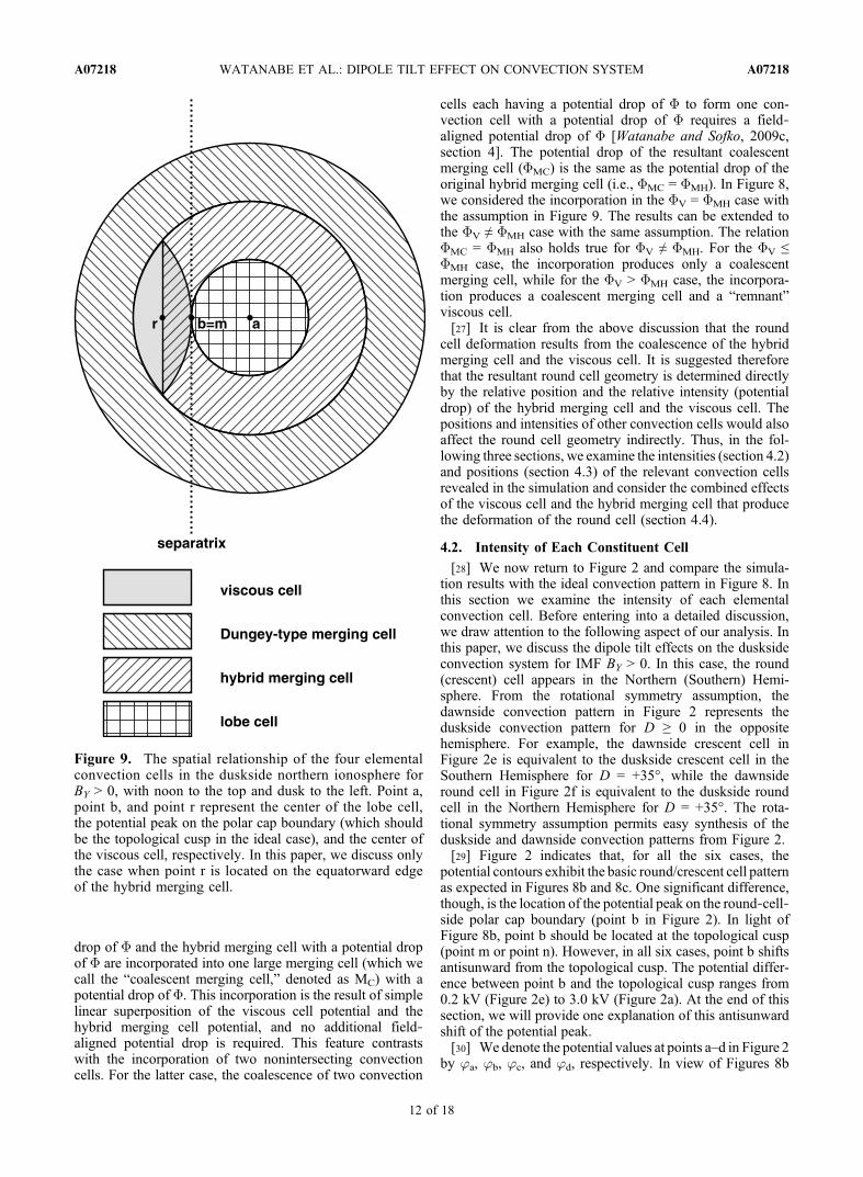
drop of F and the hybrid merging cell with a potential dropof F are incorporated into one large merging cell (which wecall the “coalescent merging cell,” denoted as MC) with apotential drop of F. This incorporation is the result of simplelinear superposition of the viscous cell potential and thehybrid merging cell potential, and no additional field‐aligned potential drop is required. This feature contrastswith the incorporation of two nonintersecting convectioncells. For the latter case, the coalescence of two convection

cells each having a potential drop of F to form one con-vection cell with a potential drop of F requires a field‐aligned potential drop of F [Watanabe and Sofko, 2009c,section 4]. The potential drop of the resultant coalescentmerging cell (FMC) is the same as the potential drop of theoriginal hybrid merging cell (i.e., FMC = FMH). In Figure 8,we considered the incorporation in the FV = FMH case withthe assumption in Figure 9. The results can be extended tothe FV ≠ FMH case with the same assumption. The relationFMC = FMH also holds true for FV ≠ FMH. For the FV ≤FMH case, the incorporation produces only a coalescentmerging cell, while for the FV > FMH case, the incorpora-tion produces a coalescent merging cell and a “remnant”viscous cell.[27] It is clear from the above discussion that the round

cell deformation results from the coalescence of the hybridmerging cell and the viscous cell. It is suggested thereforethat the resultant round cell geometry is determined directlyby the relative position and the relative intensity (potentialdrop) of the hybrid merging cell and the viscous cell. Thepositions and intensities of other convection cells would alsoaffect the round cell geometry indirectly. Thus, in the fol-lowing three sections, we examine the intensities (section 4.2)and positions (section 4.3) of the relevant convection cellsrevealed in the simulation and consider the combined effectsof the viscous cell and the hybrid merging cell that producethe deformation of the round cell (section 4.4).

4.2. Intensity of Each Constituent Cell

[28] We now return to Figure 2 and compare the simula-tion results with the ideal convection pattern in Figure 8. Inthis section we examine the intensity of each elementalconvection cell. Before entering into a detailed discussion,we draw attention to the following aspect of our analysis. Inthis paper, we discuss the dipole tilt effects on the dusksideconvection system for IMF BY > 0. In this case, the round(crescent) cell appears in the Northern (Southern) Hemi-sphere. From the rotational symmetry assumption, thedawnside convection pattern in Figure 2 represents theduskside convection pattern for D ≥ 0 in the oppositehemisphere. For example, the dawnside crescent cell inFigure 2e is equivalent to the duskside crescent cell in theSouthern Hemisphere for D = +35°, while the dawnsideround cell in Figure 2f is equivalent to the duskside roundcell in the Northern Hemisphere for D = +35°. The rota-tional symmetry assumption permits easy synthesis of theduskside and dawnside convection patterns from Figure 2.[29] Figure 2 indicates that, for all the six cases, the

potential contours exhibit the basic round/crescent cell patternas expected in Figures 8b and 8c. One significant difference,though, is the location of the potential peak on the round‐cell‐side polar cap boundary (point b in Figure 2). In light ofFigure 8b, point b should be located at the topological cusp(point m or point n). However, in all six cases, point b shiftsantisunward from the topological cusp. The potential differ-ence between point b and the topological cusp ranges from0.2 kV (Figure 2e) to 3.0 kV (Figure 2a). At the end of thissection, we will provide one explanation of this antisunwardshift of the potential peak.[30] We denote the potential values at points a–d in Figure 2

by ’a, ’b, ’c, and ’d, respectively. In view of Figures 8b

Figure 9. The spatial relationship of the four elementalconvection cells in the duskside northern ionosphere forBY > 0, with noon to the top and dusk to the left. Point a,point b, and point r represent the center of the lobe cell,the potential peak on the polar cap boundary (which shouldbe the topological cusp in the ideal case), and the center ofthe viscous cell, respectively. In this paper, we discuss onlythe case when point r is located on the equatorward edgeof the hybrid merging cell.


12 of 18

and 8c, the potential drop of each convection cell is givenby the following:

FL ¼ j’aj & j’bj; ð7Þ

FV ¼ j’dj & j’cj; ð8Þ

FMDþMC ¼ j’bj; ð9Þ

FMD ¼ j’cj; ð10Þ

FMC ¼ j’bj & j’cj; ð11Þ

where the notation FMD+MC is newly introduced here. Letus review these potentials all together. The voltage FL

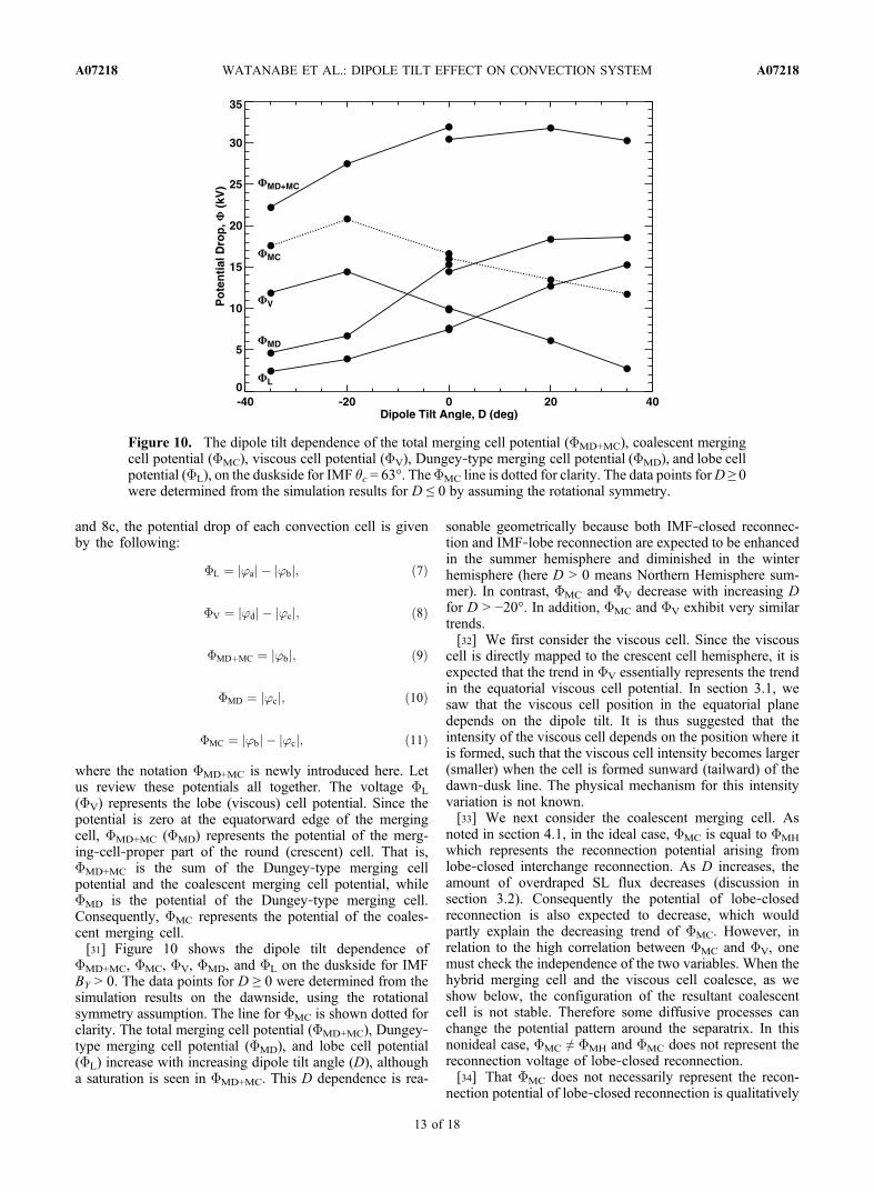
(FV) represents the lobe (viscous) cell potential. Since thepotential is zero at the equatorward edge of the mergingcell, FMD+MC (FMD) represents the potential of the merg-ing‐cell‐proper part of the round (crescent) cell. That is,FMD+MC is the sum of the Dungey‐type merging cellpotential and the coalescent merging cell potential, whileFMD is the potential of the Dungey‐type merging cell.Consequently, FMC represents the potential of the coales-cent merging cell.[31] Figure 10 shows the dipole tilt dependence ofFMD+MC, FMC, FV, FMD, and FL on the duskside for IMFBY > 0. The data points for D ≥ 0 were determined from thesimulation results on the dawnside, using the rotationalsymmetry assumption. The line for FMC is shown dotted forclarity. The total merging cell potential (FMD+MC), Dungey‐type merging cell potential (FMD), and lobe cell potential(FL) increase with increasing dipole tilt angle (D), althougha saturation is seen in FMD+MC. This D dependence is rea-

sonable geometrically because both IMF‐closed reconnec-tion and IMF‐lobe reconnection are expected to be enhancedin the summer hemisphere and diminished in the winterhemisphere (here D > 0 means Northern Hemisphere sum-mer). In contrast, FMC and FV decrease with increasing Dfor D > −20°. In addition, FMC and FV exhibit very similartrends.[32] We first consider the viscous cell. Since the viscous

cell is directly mapped to the crescent cell hemisphere, it isexpected that the trend in FV essentially represents the trendin the equatorial viscous cell potential. In section 3.1, wesaw that the viscous cell position in the equatorial planedepends on the dipole tilt. It is thus suggested that theintensity of the viscous cell depends on the position where itis formed, such that the viscous cell intensity becomes larger(smaller) when the cell is formed sunward (tailward) of thedawn‐dusk line. The physical mechanism for this intensityvariation is not known.[33] We next consider the coalescent merging cell. As

noted in section 4.1, in the ideal case, FMC is equal to FMH

which represents the reconnection potential arising fromlobe‐closed interchange reconnection. As D increases, theamount of overdraped SL flux decreases (discussion insection 3.2). Consequently the potential of lobe‐closedreconnection is also expected to decrease, which wouldpartly explain the decreasing trend of FMC. However, inrelation to the high correlation between FMC and FV, onemust check the independence of the two variables. When thehybrid merging cell and the viscous cell coalesce, as weshow below, the configuration of the resultant coalescentcell is not stable. Therefore some diffusive processes canchange the potential pattern around the separatrix. In thisnonideal case, FMC ≠ FMH and FMC does not represent thereconnection voltage of lobe‐closed reconnection.[34] That FMC does not necessarily represent the recon-

nection potential of lobe‐closed reconnection is qualitatively

Figure 10. The dipole tilt dependence of the total merging cell potential (FMD+MC), coalescent mergingcell potential (FMC), viscous cell potential (FV), Dungey‐type merging cell potential (FMD), and lobe cellpotential (FL), on the duskside for IMF *c = 63°. TheFMC line is dotted for clarity. The data points forD ≥ 0were determined from the simulation results for D ≤ 0 by assuming the rotational symmetry.


13 of 18

understood as follows. As before, we assume FMH = FV =FL = FMD = F. For simplicity, we consider a superpositionof a circular viscous cell and a circular hybrid merging cell asshown in Figure 11a. Here the Dungey‐type merging cellencompassing the viscous cell and the hybrid merging cell(see Figure 9) is not shown because it is irrelevant to thepotential superposition. In calculating the superposed po-tentials, it is convenient to set the zero potential (the refer-ence potential) at the inner edge of the Dungey‐typemerging cell (where the potential is ’ = ’0 = −F). Thus, inFigure 11, we tentatively work with a shifted potential (’′)defined as ’′ = ’ − ’0 = ’ + F. The potential at the viscous(lobe) cell center is lower by F (2F) than the inner edge ofthe Dungey‐type merging cell. Figure 11b shows thesuperposed potential pattern. In the absence of diffusion, thepotential at point b is ’′b = −F, with the lobe cell intact. Thepotential of the coalescent merging cell is FMC = F. How-ever, the segment b‐r becomes a null line of the velocityfield, and the potential pattern is unstable. Thus it is expectedthat the potentials near point b could easily transform intothe pattern in Figure 11c by a diffusive process. Thepotential at point b in the presence of diffusion (’′*b)becomes lower by D compared to the case in the absence ofdiffusion: ’′*b = ’′b − D. Therefore the coalescent mergingcell potential in the presence of diffusion (F*MC) is higherthan the original value by D (i.e., F*MC = F + D). At thesame time, the lobe cell potential in the presence of dif-fusion (F*L) is lower than the original value by D (i.e.,F*L = F − D).[35] As we saw in Figure 11, in the presence of diffusion,

the viscous cell acts to increase the potential magnitude onthe polar cap boundary. We write this relation as

j’*b j ¼ j’bj þD; ð12Þ

where ’*b (’b) represents the potential at point b in thepresence (absence) of diffusion and D is positive and afunction of FV. This potential difference D must be pro-vided by a field‐aligned potential drop somewhere in themagnetosphere. This drop is also a feature of reconnection

Figure 11. (a–c) Schematics showing how diffusion affectsthe potential peak on the round‐cell‐side polar cap boundary.Solid lines represent equipotential contours, with the label-ing numbers showing the potentials (measured in F) withrespect to the inner edge of the Dungey‐type merging cell.They equivalently represent streamlines whose flow direc-tions are indicated by arrows. As in Figure 9, point a,point b, and point r represent the center of the lobe cell, thepotential peak on the polar cap boundary, and the center ofthe viscous cell, respectively. Figure 11a shows the simplesuperposition of the convection cell elements (i.e., a lobecell L with a potential drop of F, a hybrid merging cell MH

with a potential drop of F, and a viscous cell V with apotential drop of F), while Figure 11b shows the resultantpotentials when there is no diffusion (a coalescent mergingcell MC with a potential drop of F). In the presence ofdiffusion, the potentials form a pattern in Figure 11c. HereM*C (L*) represents the coalescent merging (lobe) cell inthe presence of diffusion, and D is the potential decrementat point b due to the diffusion.


14 of 18

in a broad sense [Schindler et al., 1988] but conceptuallydistinct from the “normal” reconnection which is identifiedby plasma flow across separatrices. The coalescent mergingcell potential in the presence of diffusion (F*MC) is given by

F*MC ¼ j’*b j & j’cj ¼ FMC þD ¼ FMH þD: ð13Þ

Here FMH is the original hybrid merging cell potential andrepresents the reconnection voltage of lobe‐closed recon-nection. Therefore, F*MC overestimates the reconnectionvoltage of lobe‐closed reconnection by D. The above dis-cussion also indicates that F*L underestimates the recon-nection voltage of IMF‐lobe reconnection by D.[36] At the beginning of this section, we pointed out that

the potential peak on the round‐cell‐side polar cap boundaryshifts antisunward from the topological cusp. One probableexplanation of this displacement is the viscous cell effect inthe presence of diffusion. As we have discussed, the viscouscell acts to increase the magnitude of the potential on thepolar cap boundary. If the viscous cell is located antisun-ward of the topological cusp, the potential peak on the polarcap boundary tends to shift antisunward. This is in agree-ment with Figure 2, which shows the projected viscous cellcenter (point r) to be located antisunward of the topologicalcusp for all cases. Watanabe et al. [2007, section 6.1]suggested an alternative explanation of the potential peakshift within the framework of reconnection‐driven convec-tion; however, the viscous cell effect described above is amore reasonable interpretation.

4.3. Relative Position of the Viscous Cell and theLobe Cell

[37] In this section, we examine the relative position of theviscous cell and the hybrid merging cell. One problem hereis that we cannot observe the original hybrid merging cell in

the simulation. As an obvious alternative, we examine theposition of the lobe cell relative to the viscous cell. Thehybrid merging cell encompasses the lobe cell, and theextent of the lobe cell (the inner dotted line passing point bin Figure 2) is a good measure of the shape of the hybridmerging cell.[38] The potential contours in Figure 2 are drawn using a

polar azimuthal equidistant projection. In order to discussthe convection pattern quantitatively, we introduce Carte-sian coordinates (S, U) to Figure 2. We take the S axis alongthe SM X axis (midnight to noon) and the U axis along theSM Y axis (dawn to dusk). The origin of the coordinatesystem is the geomagnetic pole. Thus the position of anionospheric point is expressed (in degrees) by

S ¼ ð90& j)jÞ cos15ð&& 12Þ; ð14Þ

U ¼ ð90& j)jÞ sin15ð&& 12Þ; ð15Þ

where l and c are the magnetic latitude of the point indegrees and the magnetic local time of the point in hours,respectively. The value of S represents the signed distancefrom the dawn‐dusk meridian. Dipole tilt effects appear asthe sunward or antisunward motion of the points thatcharacterize the convection pattern.[39] Figure 12 shows, for the duskside northern iono-

sphere and for IMF *c = 63°, the dipole tilt dependence ofthe S values of the sunward edge of the polar cap, thetopological cusp, the sunward edge of the lobe cell, theionospheric projection of the equatorial viscous cell center,the lobe cell center, and the nightside edge of the lobe cell.Data points for D ≥ 0 were determined from the dawnsidesimulation results, assuming the rotational symmetry. Theline for the topological cusp is shown dotted for clarity. We

Figure 12. The dipole tilt dependence of the S values (see text) of the sunward edge of the polar capboundary, the Northern Hemisphere topological cusp (point m), the sunward edge of the lobe cell, theviscous cell center, the lobe cell center, and the tailward edge of the lobe cell, in the duskside northernionosphere for IMF *c = 63°. The line for the topological cusp is dotted for clarity. The data points forD ≥ 0 were determined from the simulation results for D ≤ 0 by assuming the rotational symmetry.


15 of 18

see that the S value of the sunward edge of the polar capremains almost constant irrespective of the dipole tilt, whichindicates the utility of describing the position of an iono-spheric point by this coordinate. The topological cuspmoves antisunward with increasing D as expected from thevacuum superposition model, but the magnitude of thedisplacement is only a few degrees. The sunward edge ofthe lobe cell shows nearly the same values as the topologicalcusp, which is useful information for estimating practicallythe topological cusp location from observational data. Theviscous cell center also moves antisunward with increasingD, but the antisunward shift is only a few degrees andalmost parallel to the antisunward shift of the topologicalcusp. The viscous cell center is always located antisunwardof the topological cusp, which is probably related to theantisunward shift of the potential peak on the round‐cell‐side polar cap boundary, as discussed in section 4.2.[40] We now examine the relative position of the viscous

cell and the lobe cell as originally intended. The lobe cellcenter and the sunward edge of the lobe cell moves anti-sunward with increasing D, but the relative position of thesepoints with respect to the projected viscous cell center doesnot change drastically with D. What does change signifi-

cantly with respect to the viscous cell center is the nightsideedge of the lobe cell for D ≤ 0. While, for D ] −20°, thelobe cell on the dayside is confined to a region closer tothe projected viscous cell center, the lobe cell expands to thenightside for D ∼ 0°. This expansion would be due not onlyto the geometry change with the dipole tilt change but alsoto the intensity change of the lobe cell. As Figure 10 shows,the lobe cell potential becomes very weak for D ] −20°.

4.4. Round Cell Geometry

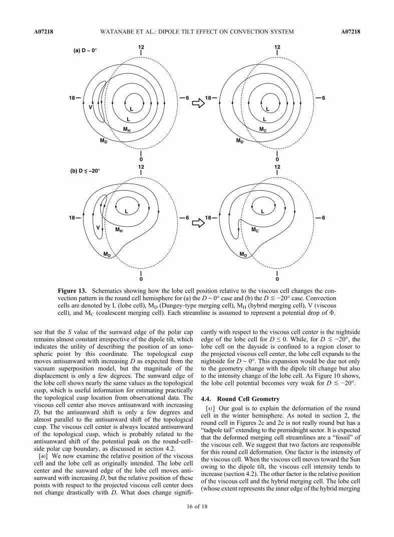
[41] Our goal is to explain the deformation of the roundcell in the winter hemisphere. As noted in section 2, theround cell in Figures 2c and 2e is not really round but has a“tadpole tail” extending to the premidnight sector. It is expectedthat the deformed merging cell streamlines are a “fossil” ofthe viscous cell. We suggest that two factors are responsiblefor this round cell deformation. One factor is the intensity ofthe viscous cell. When the viscous cell moves toward the Sunowing to the dipole tilt, the viscous cell intensity tends toincrease (section 4.2). The other factor is the relative positionof the viscous cell and the hybrid merging cell. The lobe cell(whose extent represents the inner edge of the hybrid merging

Figure 13. Schematics showing how the lobe cell position relative to the viscous cell changes the con-vection pattern in the round cell hemisphere for (a) the D ∼ 0° case and (b) the D ] −20° case. Convectioncells are denoted by L (lobe cell), MD (Dungey‐type merging cell), MH (hybrid merging cell), V (viscouscell), and MC (coalescent merging cell). Each streamline is assumed to represent a potential drop of F.


16 of 18

cell) expands to the nightside in spring, fall, and summer butis confined to the dayside in winter (section 4.3).[42] Figure 13 illustrates how the lobe cell position rela-

tive to the viscous cell affects the shape of the coalescentmerging cell, with Figure 13a showing the D ∼ 0° case andFigure 13b showing the D ] −20° case. In order toemphasize the lobe cell potential difference between the twocases, two lobe cell streamlines are drawn for the formercase. We assume that the diffusion effect is minimal so thata hybrid merging cell (MH) and a viscous cell (V), eachhaving the same potential F, are incorporated into a coales-cent merging cell (MC) with a potential drop ofF. ForD ∼ 0°,the lobe cell extends to the nightside polar cap, and conse-quently so does the hybrid merging cell. When the viscouscell is incorporated into the hybrid merging cell, the resul-tant coalescent merging cell is still round (Figure 13a). Incontrast, for D ] −20°, the lobe cell is confined to thedayside polar cap, and consequently so is the hybrid mergingcell. Because of this shrinking, the coalescent merging cellhas a tadpole‐tail‐like protrusion which is regarded as a“fossil” of the viscous cell (Figure 13b). In addition, theduskside viscous cell intensity is larger for D ] −20° thanfor D ∼ 0°. We suggest that the synergetic effect of thetwo factors − (1) the relative position of the hybrid mergingand viscous cells and (2) the intensity of the viscous cell –produces the difference between Figure 2a (round mergingcell) and Figures 2c and 2e (tadpole‐shaped merging cell).

5. Conclusions

[43] Using numerical MHD simulations, we examined theeffect of dipole tilt on the magnetosphere‐ionosphere con-vection system for IMF BY > 0 (IMF clock angle *c = 63°).The dipole tilt is parameterized by the angle D between theGSM Z axis and the SM Z axis (D is positive for borealsummer).[44] In our simulation, both reconnection‐driven convec-

tion and “viscous‐driven” convection play important roles inthe global magnetic flux circulation. When there is no dipoletilt (D = 0°), the viscous cell centers in the GSM equatorialplane are located approximately at dawn and dusk. Theazimuthal locations of the viscous cells rotate clockwise(counterclockwise) in the GSM X‐Y plane when D decreasesfrom 0° to −35° (when D increases from 0° to +35°). Wefound that this rotation is related to the geometry of thedayside separator. The equatorial crossing point of thedayside separator exhibits the same rotation in the GSM X‐Yplane as the viscous cell centers. This is because the viscouscirculation is formed inside the Dungey circulation which, inturn, is geometrically constrained by the separatrix shape.The separators demarcate the dawnside Dungey circulationand the duskside Dungey circulation, and the demarcation inthe equatorial plane is determined by the equatorial crossingpoint of the dayside separator.[45] The convection in the ionosphere is basically the

round/crescent cell pattern, but this basic pattern is affectedby the presence of the viscous cell. In the crescent cellhemisphere, the viscous cell is naturally embedded in thereconnection‐driven merging cell to form a crescent cell, butin the round cell hemisphere, the antisunward convection inthe poleward part of the viscous cell is canceled by thesunward flow of the hybrid merging cell, resulting in for-

mation of one round merging cell. When the dipole tilt issignificant (∣D∣ ^ 20°), the round cell in the winter hemi-sphere is associated with a “fossil” of the viscous cell. Wesuggest that two factors are affecting the round cell defor-mation. One is the viscous cell intensity, and the other is theextent of the lobe cell that is embedded in the hybridmerging cell. The duskside (dawnside) viscous cell tends tointensify for D ] −20° (D ^ 20°) compared to D ∼ 0°. Thelobe cell (and consequently the encompassing hybridmerging cell) in the winter hemisphere is confined on thedayside for ∣D∣ ] 20°, whereas it extends to the nightsidepolar cap for D ∼ 0°.[46] The numerical and conceptual modeling in this paper

provides a framework for interpreting observations. In fact,the round cell deformation discussed in Figure 13b is similarto the observed convection pattern in Figure 1. However, inobservations, the round cell “splits” into two. It is somewhatdoubtful that the splitting arises because the viscous cellpotential becomes larger than the hybrid merging cellpotential. Detailed analysis of the observational data andcomparison with the simulations will be required in thefuture.

[47] Acknowledgments. M. Watanabe was funded by a CanadianSpace Agency (CSA) Space Science Enhancement Program grant, a Natu-ral Sciences and Engineering Research Council (NSERC) Canada Collab-orative Research Opportunities Grant for the e‐POP satellite mission, and aCSA contract for the e‐POP mission. The motivation for the research is anunderstanding of the convection patterns measured both by the CanadianSuperDARN radars (operated with funding from both an NSERC MajorResource Support Grant and a CSA contract) and by the internationalSuperDARN radars funded by a number of national funding agencies.[48] Wolfgang Baumjohann thanks Nancy Crooker and another

reviewer for their assistance in evaluating this paper.

ReferencesAlekseyev, I. I., and Y. S. Belen'kaya (1983), Electric field in an openmodel of the magnetosphere, Geomagn. Aeron., 23, 57–61.

Axford, W. I., and C. O. Hines (1961), A unifying theory of high‐latitudegeophysical phenomena and geomagnetic storms, Can. J. Phys., 39,1433–1464.

Burch, J. L., P. H. Reiff, J. D. Menietti, R. A. Heelis, W. B. Hanson, S. D.Shawhan, E. G. Shelley, M. Sugiura, D. R. Weimer, and J. D. Winning-ham (1985), IMF BY‐dependent plasma flow and Birkeland currents inthe dayside magnetosphere: 1. Dynamics Explorer observations, J. Geo-phys. Res., 90(A2), 1577–1593, doi:10.1029/JA090iA02p01577.

Crooker, N. U. (1992), Reverse convection, J. Geophys. Res., 97(A12),19,363–19,372, doi:10.1029/92JA01532.

Crooker, N. U., J. G. Lyon, and J. A. Fedder (1998), MHD model mergingwith IMF BY: Lobe cells, sunward polar cap convection, and overdrapedlobes, J. Geophys. Res., 103(A5), 9143–9151, doi:10.1029/97JA03393.

Dorelli, J. C., A. Bhattacharjee, and J. Raeder (2007), Separator reconnectionat Earth’s dayside magnetopause under generic northward interplanetarymagnetic field conditions, J. Geophys. Res., 112, A02202, doi:10.1029/2006JA011877.

Dungey, J. W. (1961), Interplanetary magnetic field and the auroral zones,Phys. Rev. Lett., 6, 47–48, doi:10.1103/PhysRevLett.6.47.

Greene, J. M. (1992), Locating three‐dimensional roots by a bisectionmethod, J. Comput. Phys., 98(2), 194–198, doi:10.1016/0021-9991(92)90137-N.

Kivelson, M. G., and C. T. Russell (1995), Introduction to Space Physics,568 pp., Cambridge Univ. Press, New York.

Lu, G., et al. (1994), Interhemispheric asymmetry of the high‐latitude iono-spheric convection pattern, J. Geophys. Res., 99(A4), 6491–6510,doi:10.1029/93JA03441.

Parker, E. N. (1996), The alternative paradigm for magnetospheric physics,J. Geophys. Res., 101(A5), 10,587–10,625, doi:10.1029/95JA02866.

Powell, K. G., P. L. Roe, T. J. Linde, T. I. Gombosi, and D. L. DeZeeuw(1999), A solution‐adaptive upwind scheme for ideal magnetohydrody-namics, J. Comput. Phys., 154(2), 284–309, doi:10.1006/jcph.1999.6299.


17 of 18

Reiff, P. H., and J. L. Burch (1985), IMF BY‐dependent plasma flow andBirkeland currents in the dayside magnetosphere: 2. A global model fornorthward and southward IMF, J. Geophys. Res., 90(A2), 1595–1609,doi:10.1029/JA090iA02p01595.

Ridley, A. J., T. I. Gombosi, and D. L. DeZeeuw (2004), Ionospheric con-trol of the magnetosphere: Conductance, Ann. Geophys., 22, 567–584.

Russell, C. T. (1972), The configuration of the magnetosphere, in CriticalProblems of Magnetospheric Physics, edited by E. R. Dyer, pp. 1–16,Natl. Acad. of Sci., Washington, D. C.

Schindler, K., M. Hesse, and J. Birn (1988), General magnetic reconnec-tion, parallel electric fields, and helicity, J. Geophys. Res., 93(A6),5547–5557, doi:10.1029/JA093iA06p05547.

Siscoe, G. L. (1988), The magnetospheric boundary, in Physics of SpacePlasmas (1987), edited by T. Chang, G. B. Crew, and J. R. Jasperse,pp. 3–78, Sci. Publ., Cambridge, Mass.

Siscoe, G. L., G. M. Erickson, B. U. Ö. Sonnerup, N. C. Maynard, K. D.Siebert, D. R. Weimer, and W. W. White (2001a), Magnetospheric sashdependence on IMF direction, Geophys. Res. Lett., 28(10), 1921–1924,doi:10.1029/2000GL003784.

Siscoe, G. L., G. M. Erickson, B. U. Ö. Sonnerup, N. C. Maynard, K. D.Siebert, D. R. Weimer, and W. W. White (2001b), Global role of Ek inmagnetopause reconnection: An explicit demonstration, J. Geophys.Res., 106(A7), 13,015–13,022, doi:10.1029/2000JA000062.

Tanaka, T. (1999), Configuration of the magnetosphere‐ionosphere con-vection system under northward IMF conditions with nonzero IMF BY,J. Geophys. Res., 104(A7), 14,683–14,690, doi:10.1029/1999JA900077.

Tanaka, T. (2007), Magnetosphere‐ionosphere convection as a compoundsystem, Space Sci. Rev., 133(1–4), 1–72, doi:10.1007/s11214-007-9168-4.

Vasyliūnas, V. M. (2001), Electric field and plasma flow: What driveswhat?, Geophys. Res. Lett., 28(11), 2177–2180, doi:10.1029/2001GL013014.

Vasyliūnas, V. M. (2005a), Time evolution of electric fields and currentsand the generalized Ohm’s law, Ann. Geophys., 23, 1347–1354.

Vasyliūnas, V. M. (2005b), Relation between magnetic fields and electriccurrents in plasmas, Ann. Geophys., 23, 2589–2597.

Watanabe, M., and G. J. Sofko (2008), Synthesis of various ionosphericconvection patterns for IMF BY‐dominated periods: Split crescent cells,exchange cells, and theta aurora formation, J. Geophys. Res., 113,A09218, doi:10.1029/2007JA012868.

Watanabe, M., and G. J. Sofko (2009a), Role of interchange reconnectionin convection at small interplanetary magnetic field clock angles and intranspolar arc motion, J. Geophys. Res., 114, A01209, doi:10.1029/2008JA013426.

Watanabe, M., and G. J. Sofko (2009b), The interchange cycle: A funda-mental mode of magnetic flux circulation for northward interplanetarymagnetic field, Geophys. Res. Lett., 36, L03107, doi:10.1029/2008GL036682.

Watanabe, M., and G. J. Sofko (2009c), Dayside four‐sheet field‐alignedcurrent system during IMF BY‐dominated periods, J. Geophys. Res.,114, A03208, doi:10.1029/2008JA013815.

Watanabe, M., G. J. Sofko, D. A. André, T. Tanaka, and M. R. Hairston(2004), Polar cap bifurcation during steady‐state northward interplane-tary magnetic field with ∣BY∣ ∼ BZ, J. Geophys. Res., 109, A01215,doi:10.1029/2003JA009944.

Watanabe, M., K. Kabin, G. J. Sofko, R. Rankin, T. I. Gombosi, A. J. Ridley,and C. R. Clauer (2005), Internal reconnection for northward interplane-tary magnetic field, J. Geophys. Res., 110, A06210, doi:10.1029/2004JA010832.

Watanabe, M., G. J. Sofko, K. Kabin, R. Rankin, A. J. Ridley, C. R. Clauer,and T. I. Gombosi (2007), Origin of the interhemispheric potential mis-match of merging cells for interplanetary magnetic field BY‐dominatedperiods, J. Geophys. Res., 112, A10205, doi:10.1029/2006JA012179.

White, W. W., G. L. Siscoe, G. M. Erickson, Z. Kaymaz, N. C. Maynard,K. D. Siebert, B. U. Ö. Sonnerup, and D. R. Weimer (1998), Themagnetospheric sash and the cross‐tail S, Geophys. Res. Lett., 25(10),1605–1608, doi:10.1029/98GL50865.

Yeh, T. (1976), Day side reconnection between a dipolar geomagnetic fieldand a uniform interplanetary field, J. Geophys. Res., 81(13), 2140–2144,doi:10.1029/JA081i013p02140.

T. I. Gombosi and A. J. Ridley, Department of Atmospheric, Oceanic,and Space Sciences, University of Michigan, Ann Arbor, MI 48109, USA.K. Kabin and R. Rankin, Department of Physics, University of Alberta,

Edmonton, AB T6G 2M7, Canada.G. J. Sofko, Department of Physics and Engineering Physics, University

of Saskatchewan, Saskatoon, SK S7N 5E2, Canada.M. Watanabe, Department of Earth and Planetary Sciences, Graduate

School of Sciences, Kyushu University, 6‐10‐1 Hakozaki, Higashi‐ku,Fukuoka 812‐8581, Japan. ([email protected]‐u.ac.jp)


18 of 18

Documents

Dipole tilt effects on the magnetosphere ionosphere …tamas/TIGpapers/2010/2010_Watanabe.pdf · Dipole tilt effects on the magnetosphere‐ionosphere convection system during interplanetary