Direct numerical simulation ofcontrolled turbulent duct flows

Master Thesis of

Steffen Straub

At the Department of Mechanical Engineering,Institute of Fluid Mechanics

Advisors: Prof. Dr.-Ing. Bettina FrohnapfelM. Sc. Davide GattiPh.D., Docent Philipp SchlatterPh.D. Ricardo Vinuesa

Duration: June 2015 – October 2015

KIT – University of the State of Baden-Wuerttemberg and National Research Center of the Helmholtz Association www.kit.edu

Acknowledgements

I would like to thank Bettina Frohnapfel and Philipp Schlatter for giving me the possibilityto do this thesis at KTH in Stockholm. Furthermore, I need to thank Davide Gatti andRicardo Vinuesa for their support during the last months.

I would like to thank both the Professor Dr.-Ing. Erich Muller-Stiftung and the Dr.-IngWilly-Hofler-Stiftung for granting me their scholarship.

This research was conducted using the resources provided by the Swedish National Infras-tructure for Computing (SNIC) at High Performance Computing Center North (HPC2N)and at National Supercomputer Centre (NSC) at Linkoping University.

iii

I declare that I have developed and written the enclosed thesis completely by myself, andhave not used sources or means without declaration in the text.

Karlsruhe, 06.10.2015

. . . . . . . . . . . . . . . . . . . . . . . . . . . . . . . . . . . . . . . . .(Steffen Straub)

Abstract

Direct numerical simulations of controlled turbulent duct flows are conducted with thespectral element code Nek5000 (Fischer et al., 2008). The applied control technique is theharmonic oscillation of the horizontal walls in order to achieve turbulent drag reduction.To the best of the author’s knowledge, this is the first time that this control technique isnumerically investigated in a duct geometry, which is a standard choice in experiments.Different control parameters, namely the amplitude of wall velocity and the controlledarea, are tested in three different cases and their results are compared to each other andto the uncontrolled flow. Two effects of this control technique in a rectangular duct areinvestigated: the effect on drag reduction and the effect on the secondary motions inducedby the corners. Additionally, selected statistics of the mean flow are evaluated in order tounderstand the impact of the moving walls on the turbulent flow.It is found that the secondary motions are strongly amplified and modified in shape andlocation compared to the uncontrolled turbulent duct flow. One of the two counter ro-tating streamwise vortices at the corner is strengthened and pushes the other one closerto the core region. In the case of partially moving horizontal walls an additional pair ofcounter rotating streamwise vortices is generated.The achieved drag reduction levels are poor compared to the results in a channel. The onlypositive drag reduction achieved is 3% in one case where the corresponding results in thechannel are 19%. The case with higher amplitude of wall velocity shows a drag increase of10% and the case with reduced controlled area only in the centre of the duct yields dragincrease of 1%. It is shown that these low or even negative levels of drag reduction are aresult of the poor performance at the sides of the controlled region.

Direkte numerische Simulationen von kontrollierten turbulenten Stromungen werden imKanal unter Berucksichtigung der Seitenwande mit dem spectral element code Nek5000Fischer et al. (2008) durchgefuhrt. Die verwendete Technik zur Stromungskontrolle ist dieharmonische Oszillation der horizontalen Wande zum Zwecke der Reduktion der turbulen-ten Reibung. Nach bestem Wissen des Autors ist dies das erste Mal in der diese Technikzur Stromungskontrolle in in einem Kanal mit Seitenwanden numerisch untersucht wird.Verschiedene Parameter der Stromungskontrolle, und zwar die Wandgeschwindigkeitsam-plitude und die kontrollierte Flache, werden in drei unterschiedlichen Fallen getestet undihre Ergebnisse untereinander und mit dem unkontrollierten Fall verglichen. Zwei Effektedieser Technik zur Stromungskontrolle im rechteckigen Kanal mit Seitenwanden werdenuntersucht: der Effekt auf die Reibungsminderung und der Effekt auf die Sekundarstro-mungen, welche durch die Ecken im Kanal erzeugt werden. Zusatzlich werden einigegemittelte Statistiken ausgewertet um die Auswirkung der bewegten Wande auf die tur-bulente Stromung zu verstehen.Die Sekundarstromung wird verglichen zum unkontrollierten Fall stark angefacht und inGestalt und Lage verandert. Einer der entgegengesetzt rotierenden Wirbeln in der Eckewird verstarkt und verdrangt den anderen Wirbel naher ins Zentrum des Kanals. Im Fallevon nur teilweise kontrollierten horizontalen Wanden wird ein weiteres Paar von entge-gengesetzt rotierenden Wirbeln erzeugt.Das erzielte Niveau der Reibungsminderung ist verglichen zu den Ergebnissen im Kanalohne Seitenwande sehr gering. Die einzige positive Reibungsminderung, die erreicht wirdbetragt 3% in einem Fall bei dem 19% im Kanal ohne Seitenwande erreicht wird. Der Fallmit hoherer Wandgeschwindigkeitsamplitude ergibt eine Reibungserhohung von 10% undim Falle verkleinerter Flache der Stromungskontrolle nur im Zentrum des Kanals ergibtsich eine Reibungserhohung von 1%. Es wird gezeigt, dass diese niedrigen oder sogarnegativen Werte der Reibungsminderung ein Resultat der schlechten Performance an denSeiten des kontrollierten Gebiets sind.

v

Contents

Acknowledgements iii

Abstract v

1. Introduction 11.1. Motivation . . . . . . . . . . . . . . . . . . . . . . . . . . . . . . . . . . . . 1

1.2. State of the art . . . . . . . . . . . . . . . . . . . . . . . . . . . . . . . . . . 2

1.3. Objectives of this thesis . . . . . . . . . . . . . . . . . . . . . . . . . . . . . 3

1.4. Structure of the thesis . . . . . . . . . . . . . . . . . . . . . . . . . . . . . . 3

2. Fundamentals 42.1. Governing equations for incompressible fluid mechanics . . . . . . . . . . . 4

2.2. Numerical solution to the incompressible Navier–Stokes equations . . . . . . 6

2.3. Channel flow . . . . . . . . . . . . . . . . . . . . . . . . . . . . . . . . . . . 7

2.4. Duct flow . . . . . . . . . . . . . . . . . . . . . . . . . . . . . . . . . . . . . 11

2.5. Control technique . . . . . . . . . . . . . . . . . . . . . . . . . . . . . . . . . 12

3. Numerical methods 143.1. Weighted residual techniques: Galerkin method . . . . . . . . . . . . . . . . 14

3.2. Spatial discretization . . . . . . . . . . . . . . . . . . . . . . . . . . . . . . . 17

3.3. Temporal discretization . . . . . . . . . . . . . . . . . . . . . . . . . . . . . 20

3.4. Parallelization . . . . . . . . . . . . . . . . . . . . . . . . . . . . . . . . . . . 21

4. Investigated cases 224.1. Channel cases . . . . . . . . . . . . . . . . . . . . . . . . . . . . . . . . . . . 22

4.2. Duct cases . . . . . . . . . . . . . . . . . . . . . . . . . . . . . . . . . . . . . 24

5. Validation 275.1. Uncontrolled channel flow . . . . . . . . . . . . . . . . . . . . . . . . . . . . 27

5.2. Controlled channel flow . . . . . . . . . . . . . . . . . . . . . . . . . . . . . 29

6. Results 316.1. Mean statistics . . . . . . . . . . . . . . . . . . . . . . . . . . . . . . . . . . 31

6.2. Secondary flow . . . . . . . . . . . . . . . . . . . . . . . . . . . . . . . . . . 42

6.3. Wall shear stress and drag reduction . . . . . . . . . . . . . . . . . . . . . . 46

7. Conclusion and Outlook 51

Symbols and Abbreviations 54

List of Figures 57

List of Tables 59

vii

Contents viii

Bibliography 60

Appendix 63A. Best fit property . . . . . . . . . . . . . . . . . . . . . . . . . . . . . . . . . 63B. Lagrangian interpolants . . . . . . . . . . . . . . . . . . . . . . . . . . . . . 64

viii

1. Introduction

1.1. Motivation

Our daily life is surrounded by many different kinds of wall-bounded flows. This couldbe for instance the flow around a car, bus, metro or any other means of transportation.If you go on vacation and take the plane, the flow around its wings is the crucial factorwhich enables the plane to fly. Another example is the flow through pipes. There are hugepipelines for the transportation of gas, oil or water for instance. All those flows and manymore have one thing in common: they produce drag.For some cases the drag is beneficial or even essential, as for example for a parachute, butfor many other flows drag is an unwanted by-product. Modern vehicles such as cars, planesor ships do not produce as much drag as they did in the beginning of their development.For those applications, as for flow through pipelines, less drag often means less powerconsumption. For instance, if one applies a specific pressure gradient to push fluid througha section of a pipe, the same mass flow rate can be achieved with a smaller pressure gradientwhen drag is reduced. On the other hand drag, reduction can also result in an increasedmass flow rate by keeping the pressure gradient constant. In both cases the results arebeneficial. Reducing the power input or increasing the mass flow rate in the example aboveleads to a higher efficiency of the device. A higher efficiency is not only beneficial in afinancial point of view but it improves ecological aspects, too. Kim (2011) claims that wecould save 38 billion Dollar per year if the fuel consumption of worldwide shipping wasreduced by 30 % (considering 2003 figures of fuel consumption and 60 Dollar per barrel).A reduction of fuel consumption would also reduce exhaust gases and carbon dioxide.This is where the science of flow control comes in (Gad-el Hak, 2000). In this branch offluid dynamics one tries to manipulate the natural behaviour of the flow in a beneficialway (Pope, 2010). For instance, improved mixing between fluids, improved heat transferor methods for drag reduction are investigated. The focus of this thesis is on a simpletechnique for drag reduction. Since most engineering flows are turbulent, the goal is toreduce turbulent drag.One can distinguish between laminar and turbulent flows. The cases considered hereare turbulent flows. It is difficult to give a proper definition of turbulence. Some of itscharacteristics however can help to clarify its meaning.

1

1. Introduction 2

According to Tennekes and Lumley (1972) they are:

• Irregularity, randomness

• Mixing: increased rates of momentum, heat and mass transfer

• Large Reynolds number

• Three-dimensional vorticity fluctuations: turbulent flows are rotational

• Dissipation: energy is needed to sustain turbulence

• Continuum: smallest scales are still larger than molecular length scales

• Turbulence is a feature of the flow not the fluid

A simple, yet imperfect definition of turbulence is given by Kundu et al. (2012) as ”adissipative flow state characterized by nonlinear fluctuating three-dimensional vorticity”.Due to the mentioned characteristics of increased mixing and dissipation, usually turbu-lent flows are accompanied by higher drag compared to laminar flows. This additionalcomponent of drag for turbulent flows is referred to as turbulent drag.

1.2. State of the art

The different kinds of drag reduction mechanisms for wall-bounded flows can be groupedinto either active or passive techniques (Gad-el Hak, 2000). The difference between those isthat the former needs additional power input and the latter does not. For active techniquesone can further differentiate between techniques which measure specific flow quantitiesand change their parameters accordingly (reactive) and techniques which do not react onchanges in the flow (predetermined).A well known passive technique for drag reduction is the use of riblets. This technique,which is inspired by the microgrooves of shark skin, has been shown to reach drag re-duction levels of about 10 % (Bechert et al., 1997; Garcia-Mayoral and Jimenez, 2011).For a wing-body Viswanath (2002) found 2 − 3% total drag reduction based on limitedwind tunnel data. One major advantage of passive techniques is that no additional powerinput is needed. However, the amount of drag reduction achieved so far is much smallercompared to active techniques. Predetermined active techniques do not require complexsensors and actuators as the reactive techniques do. They are simpler and cheaper thanthe reactive techniques.One promising predetermined active control technique to reduce drag in channel and pipeflows is the spanwise oscillatory motion of the walls. This technique will be investigatedin the present thesis. Jung et al. (1992) were the first to investigate this phenomenonby direct numerical simulations. They found that sustained turbulent drag reduction of10 % to 40 % compared to the uncontrolled case was possible. Since then many experi-mental and numerical studies have been conducted to achieve a better understanding ofthe mechanisms behind this phenomenon. Laadhari et al. (1994) were able to show exper-imentally the effects of a spanwise oscillating wall for turbulent boundary layers. Theirresults are generally in good agreement with Jung et al. (1992). The first of many arti-cles published by Quadrio and co-workers (Baron and Quadrio, 1995) confirms Jung et al.(1992)’s findings of 40 % drag reduction. They also take into account the power inputneeded to generate the wall motion and show that potential overall savings are possible.A simple model is proposed which states that the spatial coherence between streamwisevortices and low-speed streaks is disrupted causing the drag reduction. In another exper-imental investigation Choi et al. (1998) confirmed the previous results by achieving 45 %drag reduction in their wind-tunnel experiment. They propose a conceptual model thatexplains the decrease of the mean velocity-gradient close to the wall by a net spanwise

2

1. Introduction 3

vorticity generated by the periodic Stokes layer. A new parameter which combines theinfluence range and the acceleration of the Stokes layer was introduced by Choi and Xu(2002) to obtain a simple equation that allows to estimate drag reduction rates. Anotherarticle by Quadrio’s group (Quadrio and Ricco, 2004) identifies the optimal values for wallvelocity amplitude and time period for harmonic wall oscillation by a parametric study.They show their results in drag reduction maps. Further attempts to shed some light onthe mechanism for skin-friction drag reduction were done by Ricco et al. (2012). They lookat the mean energy balance, turbulent kinetic energy balance and the turbulent enstrophybalance to find one vorticity production term that is dominant and largely responsiblefor drag reduction. In a recent article Yakeno et al. (2014) claim that drag reduction ismostly due to suppression of ejection events by spanwise shear. Moreover, their resultssuggest a link between the suppression of ejection events and Ricco et al. (2012)’s vorticityproduction term.Even though many experimental and numerical investigations have already been conductedthe phenomenon behind this drag reduction technique is still not fully understood.

1.3. Objectives of this thesis

The objective of this thesis is to simulate the effects of the aforementioned flow controltechnique in a more realistic geometry than the standard plane channel. To the best of theauthor’s knowledge all previous direct numerical simulations were done in such a channelwith periodic boundary conditions in spanwise direction (and few simulations performed inboundary layers, for example Skote (2011); Lardeau and Leschziner (2013)). This artificialperiodicity strongly simplifies the simulations. However, in experiments side walls need toconfine the flow region.Therefore, two different effects are being investigated. The first one is the effect of theside walls on the performance of the flow control technique. Gatti et al. (2015) find adiscrepancy between their experimental results and results generated by direct numericalsimulations which might be caused by not taking into account the effect of the side walls.The second one is the effect of the applied flow control technique on secondary motionsproduced at the duct corners. This mechanism is not present in the channel but in theduct and affects the mean flow (Vinuesa et al., 2014).To be able to take the side walls into account a highly parallelized code using the spectralelement method is used: Nek5000 (Fischer et al., 2008).

1.4. Structure of the thesis

After this introduction into the topic, chapter 2 presents the governing equations for incom-pressible fluid mechanics and the Reynolds-averaged Navier–Stokes equations as a generalnumerical method to tackle this set of nonlinear partial differential equations. Further-more, the channel flow is investigated more closely and some specific features of the ductflow are mentioned. Finally, the applied control technique is presented.Chapter 3 deals with the numerical methods used for the simulations in this thesis. Thespectral element method is introduced with two model problems and the spatial and tem-poral discretization is shown. All the investigated cases are described in chapter 4. Thesetup for each channel and duct flow is described.A comparison between data from the literature, a pseudo spectral code and results gener-ated with the spectral element code Nek5000 is given in chapter 5 in order to validate theimplementation of the channel cases. The major results are presented in chapter 6. Theyare explained and discussed. A short conclusion of the results and an outlook on somepossible continuing investigations is given in chapter 7.

3

2. Fundamentals

This chapter is about the necessary fundamentals for the present thesis. First, the gov-erning equations for incompressible flows, the Navier–Stokes equations, are presented. Formany cases, these need to be solved numerically. One approach, the Reynolds-averagedNavier–Stokes equations, is presented in the subsequent section and two other approaches,the direct numerical simulation and the large eddy simulation are mentioned.The third section introduces the channel flow and the Reynolds-averaged Navier–Stokesequations for this important case before some specific features in the duct flow are men-tioned. The topic of the last section in this chapter is the investigated control technique.

2.1. Governing equations for incompressible fluid mechanics

Fluid mechanics can be considered as a branch of continuum mechanics. As long as theratio of the mean free path of molecules and the length scale of interest is small enoughthat the Knudsen number is Kn 1, the continuum assumption holds (Kundu et al.,2012). This means that the governing equations of continuum mechanics determine thequantities of interest. For incompressible flows those quantities are the three componentsof the velocity vector u, v, w and the pressure p as a Lagrangian multiplier to fulfil thecontinuity equation.The governing equations of incompressible flows are the conservation of mass and mo-mentum. The differential form of mass conservation, also known as continuity equation,is

∂ρ

∂t+

∂

∂xi(ρui) = 0, (2.1)

Dρ

Dt+ ρ

∂ui∂xi

= 0. (2.2)

The Einstein summation convention is used and ui, xi are the i-components of the in-stantaneous velocity field and the cartesian coordinate respectively. The indices i rangefrom 1 to 3 in three dimensions. Time is denoted by t and ρ is the density. The materialderivative

D(·)Dt≡ ∂(·)

∂t+ ui

∂(·)∂xi

(2.3)

of the density vanishes for incompressible flows and when the density is constant. Thedifference between incompressible and constant density is that for constant density both

4

2. Fundamentals 5

partial derivatives are zero whereas for an incompressible fluid only the sum of both partialderivatives needs to vanish (Kundu et al., 2012). In this thesis the density is assumed tobe constant. Thus, the continuity equation for incompressible flows reduces to

∂ui∂xi

= 0. (2.4)

The differential form of the momentum equation, also known as Cauchy’s equation ofmotion, is (Kundu et al., 2012)

ρDujDt

= ρ

(∂uj∂t

+ ui∂uj∂xi

)= ρfj +

∂σij∂xi

. (2.5)

The j-component of the body force is denoted by fj and σij is the stress tensor. In gen-eral, the four unknown quantities u1, u2, u3 and p are all dependent in space and time, forexample u1 = u1(x1, x2, x3, t) as well as the body force fj = fj(x1, x2, x3, t). For brevitythis dependency is omitted here. The body force could be for instance the gravitationalacceleration or the Lorentz force in magnetohydrodynamics. Hereafter, the body force fjwill be omitted because the influence of gravity will be neglected for the present thesis andthere are no other body forces acting on the fluid.The constitutive equation which relates the stress tensor σij with the four unknown quan-tities p, u1, u2, u3 for an incompressible Newtonian fluid is given by

σij = −pδij + µ

(∂ui∂xj

+∂uj∂xi

). (2.6)

The Kronecker delta δij is used which is zero for all combinations of i and j except fori = j where it is 1. The dynamic viscosity is a material property. It is denoted by µand assumed to be constant for the present thesis. The combination of the constitutiveequation 2.6 and the momentum equation 2.5 with the use of the continuity equation 2.4yields the Navier–Stokes equations (NSE) for an incompressible Newtonian fluid

ρ

(∂uj∂t

+ ui∂uj∂xi

)= − ∂p

∂xj+ µ

∂2uj∂x2

i

. (2.7)

Together with the continuity equation 2.4 these four partial differential equations are thegoverning equations for any incompressible, Newtonian fluid without body forces.

5

2. Fundamentals 6

2.2. Numerical solution to the incompressible Navier–Stokesequations

Since there are only few analytical solutions to these partial differential equations (PDEs)for special cases, different numerical approaches to solve these equations exist. This sectiondescribes the Reynolds-averaged Navier–Stokes (RANS) equations which are often usedto find a numerical solution by introducing closure terms. Direct numerical simulations,which do not need these closure terms, are mentioned together with their limitations. Athird approach, the large eddy simulation (LES) is also briefly mentioned.

Due to the randomness of turbulent flows statistical approaches are used to describe theflow. One well-known statistical approach to the NSE are the RANS equations. Thefirst step to derive the RANS equations is to decompose the instantaneous dependent-fieldvariables (velocity and pressure) into a mean (Uj , P ) and fluctuating part (u′j , p

′), theso-called Reynolds decomposition

uj = Uj + u′j , (2.8)

p = P + p′, (2.9)

where the mean velocity could be defined as the average in time

Uj(x1, x2, x3) = 〈uj(x1, x2, x3, t)〉 = limT→∞

1

T

∫ T

0uj(x1, x2, x3, t)dt. (2.10)

The brackets 〈·〉 are used to denote the averaging operator, in this case the average intime. The same averaging is applied to the instantaneous pressure field.Insertion of the decomposed velocity 2.8 into the continuity equation 2.4 and averagingshows that the mean velocity field and the fluctuating velocity field both have to satisfythe divergence-free condition

∂Ui∂xi

= 0, (2.11)

∂u′i∂xi

= 0. (2.12)

Decomposition and insertion of velocity and pressure with subsequent averaging results inthe RANS equations for an incompressible, Newtonian fluid

ρ

(∂Uj∂t

+ Ui∂Uj∂xi

)= − ∂P

∂xj+ µ

∂2Uj∂x2

i

− ρ ∂

∂xi〈u′iu′j〉. (2.13)

A solution to the four PDEs 2.11 and 2.13 for the dependent-field variables U1, U2, U3

and P can be found only when the unknown term 〈u′iu′j〉 is modelled. This term is oftenreferred to as the Reynolds stress (sometimes including the density).There is a huge variety of different models, some well-known ones are the mixing-lengthmodel and the k - ε-model which both belong to the class of turbulent-viscosity models.

Another approach that does not need any modelling is the direct numerical simulation.This approach is conceptually easier than the RANS equations combined with modellingterms because there is no additional modelling required and the NSE are solved directlyinstead of the RANS equations. It has to be noted that this is only possible if all relevantlength scales are properly resolved. What seemed to be an ”exciting prospect” about 50years ago (Corrsin, 1961) is nowadays possible due to some major progress in algorithmsand computational resources. In 1987 the first DNS of a channel flow was done by Kim

6

2. Fundamentals 7

et al. (1987). Since then many flows in simple geometries were investigated by DNS andtheir results are often used as a reference due to their good agreement with experimentalresults.

The third approach, large-eddy simulation, can be considered as a mixture between RANSand DNS. For the large, energy containing scales the filtered NSE are solved directlywhereas the residual scales are being modelled.

To conclude, the DNS is the most accurate of the three approaches because no mod-elling is involved which could introduce errors. However, this approach is much moreexpensive in terms of computational time. A very high resolution is needed to resolve thedissipative scales. Since the necessary resolution can be related to the Reynolds number(Re), it can be shown that DNS is only feasible for low Reynolds numbers. A definition ofthe Reynolds number for a channel flow will be given in section 2.3. Compared to RANS,DNS is much more time-consuming and needs much more computational resources. Thus,it is mostly used for research.Solving the RANS equations instead is faster because the resolution does not need to be ashigh as for a DNS and the Reynolds stress is modelled. Careful consideration of the mostsuitable model for different cases is needed because the accuracy is not as good as with aDNS. Furthermore, there is no model which describes every flow scenario better than allthe others. Due to its short run-time and applicability to higher Reynolds numbers, thisis the standard industrial approach.In between those two there is the LES. The filtered NSE are solved directly and the resid-ual scales are modelled which leads to higher accuracy than RANS but not as good as DNSand higher computation time than RANS but not as much as DNS, all depending on theratio of filtered and residual scales. This approach is also applicable to higher Reynoldsnumbers but still mostly used in research because industrial fluid mechanics is much moredriven by time-constraints.

2.3. Channel flow

The turbulent channel flow is one of the simplest wall-bounded turbulent flows, why muchnumerical and experimental research has been done investigating this kind of flow. Someimportant definitions and theoretical results for the channel flow are given by Pope (2010,chapter 7.1) and will be summarized in this section.A generic sketch of a duct flow is given in figure 2.1 (a). The flow is confined between anupper and a lower wall and two side walls. If the width of the duct B is large compared toits height H the flow far away from the side walls is thought to be statistically independentof the spanwise position z. The independence of spanwise position is modelled numericallyby using periodic boundary conditions at the side walls to replicate the infinite width B.This is referred to as a channel flow and depicted in figure 2.1 (b). Streamwise, wall-normaland spanwise direction are x, y, z respectively. They are corresponding to x1, x2, x3 inequations using index notation. The streamwise, wall normal and spanwise velocity aredenoted by u, v, w or u1, u2, u3 respectively. The geometry of the channel is defined bya length L and a channel height of H = 2h with channel half height h. An additionalparameter for the duct is its width B which is considered to be infinite for the channel.

A characteristic length scale for the channel flow is the channel half height h. As a char-acteristic velocity one can choose for instance the mean bulk velocity Ub which is definedas the spatially averaged mean streamwise velocity in the y − z plane

Ub =1

HB

∫ H

0

∫ B

0U(y)dzdy =

1

H

∫ H

0U(y)dy =

1

h

∫ h

0U(y)dy. (2.14)

7

2. Fundamentals 8

z

yx

B

Flow

(a)

z

yx

LH=2h

Flow

(b)

Figure 2.1.: Schematic drawing of (a) duct and (b) channel flow.

In a fully developed channel flow the mean streamwise velocity only depends on wall-normal distance y and is symmetric around y = h.The characteristic length scale h and velocity scale Ub can be used to define a characteristictime scale h/Ub and a characteristic pressure ρU2

b . Those characteristic scales are used tonon-dimensionalize velocity, time, cartesian coordinate and pressure:

u∗j =ujUb

, t∗ =tUbh

, x∗i =xih

, p∗ =p

ρU2b

. (2.15)

Here, the non-dimensionalized variables are denoted with the superscript ∗. Substitu-tion of those non-dimensionalized quantities with those from equation 2.7 and equation2.4 yields the non-dimensionalized NSE and continuity equation according to this non-dimensionalization

∂u∗j∂t∗

+ u∗i∂u∗j∂x∗i

= −∂p∗

∂x∗j+

1

Reb

∂2u∗j∂x∗i ∂x

∗i

, (2.16)

∂u∗i∂x∗i

= 0. (2.17)

One of the most important dimensionless quantities for this case emerges, the bulk Reynoldsnumber

Reb ≡hUbν. (2.18)

There are several definitions for a Reynolds number in the channel flow which depend onthe choice of the characteristic scales. If the mean centreline velocity Uc = U(y = h) ischosen as a characteristic velocity instead of Ub the Reynolds number is defined with thecentreline velocity

Rec ≡hUcν. (2.19)

The Reynolds number can be interpreted as the ratio of inertial forces over viscous forces.The value of Reb determines if the flow is either laminar Reb < 1350 or turbulent Reb >1800 with transitional effects up to Reb = 3000 (Pope, 2010).The non-dimensionalized form of the NSE 2.16 and continuity equation 2.17 facilitatesthe transferability of different setups. As long as geometrical similarity is ensured andthe dimensionless quantities such as the Reynolds number are kept constant, all non-dimensionalized flow quantities are the same (Spurk, 2010). This is essential to experimentson prototypes in wind-tunnel facilities and also on the setup of numerical experiments.The non-dimensionalized parameters will be used for all the investigated cases in chapter 4.The following presentation of the NSE and continuity equation for the channel flow willbe using dimensional quantities again, according to Pope (2010)’s notation.

8

2. Fundamentals 9

The governing equations can be specialized for a channel flow. The mean continuityequation 2.11 simply yields V = 0 because U is independent of x in a fully developed flow,W = 0 and no-slip boundary conditions are assumed.The mean momentum equation for a steady channel flow in wall-normal direction y reads

0 =1

ρ

∂P

∂y+

∂

∂y〈v′v′〉, (2.20)

0 =1

ρ(P − Pw) + 〈v′v′〉, (2.21)

where equation 2.21 is derived by integration in wall-normal direction and 〈v′v′〉|y=0 = 0.Pw is the mean pressure at the wall y = 0 and is only dependent on streamwise positionx. Thus, one can infer that

∂P

∂x=

dPwdx

, (2.22)

which can be used to rewrite the streamwise momentum equation

0 = νd2U

dy2− d

dy〈u′v′〉 − 1

ρ

∂P

∂x, (2.23)

0 =d

dy

(µ

dU

dy− ρ〈u′v′〉

)− dPw

dx. (2.24)

The kinematic viscosity ν is defined as ν ≡ µ/ρ. The combination of viscous shear stressand turbulent shear stress can be identified as the total shear stress

τ = µdU

dy− ρ〈u′v′〉. (2.25)

The turbulent shear stress −ρ〈u′v′〉 is one component of the Reynolds stress tensor. Equa-tion 2.24 has a simple solution because τ = τ(y) is only dependent on wall-normal locationy whereas Pw = Pw(x) is only dependent on the streamwise location x. Thus, both deriva-tives need to be constant. With the definition of the wall shear stress as

τw ≡ τ(y = 0) ≡ µ dU

dy

∣∣∣∣y=0

(2.26)

this constant is defined as τw. An often used non-dimensional parameter formed of τw isthe skin-friction coefficient

Cf =2τwρU2

b

. (2.27)

Together with the symmetry condition at y = h, which implies that τ(y = h) = 0, a linearprofile of the total shear stress is found:

τ(y) = τw

(1− y

h

). (2.28)

The previously defined wall shear stress (2.26) and the viscosity are the most importantparameters close to the wall because viscous effects are dominant in this region. To comeup with a different set of scaling parameters for the region close to the wall, the frictionvelocity or wall shear stress velocity is defined as

uτ =

√τwρ. (2.29)

Based on the friction velocity another Reynolds number Reτ can be defined as

Reτ ≡uτh

ν. (2.30)

9

2. Fundamentals 10

The friction velocity uτ and the kinematic viscosity ν can be used as scaling parametersclose to the wall. They are referred to as viscous scales or inner scales. For the region faraway from the wall, where viscous effects are negligible, there are the centreline velocityUc or the bulk velocity Ub and channel half height h as scaling parameters. These arereferred to as outer scales.

A dimensional analysis of the channel flow reveals that the six parameters which fullydescribe the flow (U , uτ , ρ, ν, h, y) can be reduced to three non-dimensional quantities.Instead of using the mean streamwise velocity its wall-normal gradient is used. The resultof the dimensional analysis is the relation between the three non-dimensional quantities,

dU

dy

y

uτ= Φ

(yuτν,y

h

), (2.31)

where Φ is a universal non-dimensional function.In close proximity to the wall the third non-dimensional quantity is neglected (y/h 1).This region is called the inner layer and equation 2.31 can be simplified and scaled withthe viscous scales,

du+

dy+=

1

y+Φ1(y+). (2.32)

The viscous scaling of the mean streamwise velocity U and the wall-normal direction y isgiven by

u+ =U

uτ, (2.33)

y+ =yuτν. (2.34)

The integral yields the well known law of the wall

u+ =

∫ y+

0

1

yΦ1(y)dy, (2.35)

where the right-hand side is only dependent on y+. For small values of y+ a Taylor seriesexpansion of the right-hand side shows that the integral can be approximated by y+. Thisyields the expression for the viscous sublayer (y+ < 5)

u+ = y+. (2.36)

Still in the inner layer (y/h < 0.1) but for larger values of y+, viscous effects become moreand more negligible. This means that the universal non-dimensional function Φ1 also losesits dependence on y+ and becomes a constant κ−1. This constant is the von Karmanconstant. Using this fact in equation 2.32 and integrating gives the logarithmic law of thewall,

du+

dy+=

1

κy+, (2.37)

u+ =1

κln(y+) + C. (2.38)

The two constants κ and C are suggested by (Pope, 2010) to take the following values:

κ = 0.41, C = 5.2. (2.39)

10

2. Fundamentals 11

2.4. Duct flow

For an infinitely wide duct the flow in the centre can be be described by the equationsfor the channel flow presented above. If the width is not much larger than the height theeffect of the side walls is not negligible and the assumption of spanwise independence isnot valid anymore.Two features which are absent in the channel are the secondary flow and the boundarylayers growing on the side walls. The latter are responsible for an increased streamwisevelocity at the core of the duct when compared to a channel with the same bulk velocity.This is due to the decreased streamwise velocity in the vicinity of the side walls which inexchange leads to an increased streamwise velocity in the core region. This leads to anincrease in wall shear stress at the centreplane (z = 0) of the duct (Vinuesa et al., 2014).The other remarkable feature of a turbulent duct flow is the presence of the secondaryflow field. According to Oertel jr. (2012) this cross-flow arises as a result of fluid beingtransported to the core at regions of high wall shear stress and in exchange at regions oflow wall shear stress, for instance at the corners, fluid moves towards the wall. This leadsto a pattern of one pair of counter rotating vortices at each corner of the rectangular ductas can be seen for instance in Gessner and Jones (1965). The formation of those vorticescan be further understood by investigating the mean streamwise vorticity, Ω, transportequation for a fully developed straight duct flow (Gavrilakis, 1992),

V∂Ω

∂y+W

∂Ω

∂z− ν

(∂2

∂y2+

∂2

∂z2

)Ω

= − ∂2

∂y∂y

(〈w′2〉 − 〈v′2〉

)−(∂2

∂y2− ∂2

∂z2

)〈v′w′〉,

(2.40)

where the mean streamwise vorticity is given by

Ω =∂W

∂y− ∂V

∂z. (2.41)

The terms on the left-hand side of equation 2.40 are the mean flow convection and viscousdiffusion of the mean streamwise vorticity. The two terms on the right-hand side con-tribute to the production of the mean streamwise vorticity, which is why this secondaryflow is also known as Reynolds-stress-induced secondary flow (or Prandtl’s second kindaccording to Prandtl (1926)). Therefore, this type of secondary flow only arises for tur-bulent flows and is consequently non-existent for a laminar flow (Gessner and Jones, 1965).

As pointed out by Vinuesa et al. (2014), the two three-dimensional effects present inthe duct, i.e. side wall boundary layers and secondary flow, have competing effects onthe flow. The boundary layer growth from the side walls increases momentum in the coreregion and consequently the wall shear stress at the centre of the duct is increased. Incontrast, the secondary motions transport momentum from the core region towards thecorner bisectors, thus, decreasing the wall shear stress in the centre.

One interesting quantity to quantify the magnitude of the secondary flow is its kineticenergy defined as

K :=1

2(V 2 +W 2), (2.42)

which will be used later to assess the differences in the secondary flow field between theuncontrolled and controlled cases.

11

2. Fundamentals 12

2.5. Control technique

The aim of the applied flow control technique in this thesis is to achieve high drag reduction.Fukagata et al. (2002) show that the skin-friction coefficient for a fully developed turbulentchannel flow driven at constant flow rate can be decomposed into a laminar and a turbulentcontribution

Cf =12

Reb+ 12

1∫0

2(1− y)(−〈u′v′〉)dy. (2.43)

This equation shows why the skin-friction drag of the fully developed turbulent channelis usually much larger than that of the laminar one since the second term vanishes forthe latter and is usually positive. Therefore, in order to achieve turbulent drag reduction−〈u′v′〉 is desired to decrease.

The flow control technique used for the simulations in this thesis is the harmonic os-cillation of the upper and lower walls. This technique was chosen because it is simple, easyto implement and leads to high drag reduction. Drag reduction DR is defined by

DR :=Cf,0 − Cf,c

Cf,0, (2.44)

where Cf,0 and Cf,c denote the skin-friction coefficient of the uncontrolled reference caseand the controlled case, respectively.

The harmonic oscillation of the horizontal walls is similar to Stokes’ second problem.Even though the solution to Stokes’ second problem is only a solution to the 2D laminarproblem it agrees very well with the phase averaged spanwise velocity of controlled channelcases as is shown by Choi and Xu (2002) and Choi (2002) which is another reason whythis problem is presented here.Stokes’ second problem is one of the few flows that can be described by an analyticalsolution to the Navier–Stokes equations for the laminar case. It is characterized by aninfinite flat plate that oscillates in a harmonic motion under an initially quiescent fluid.This is depicted in figure 2.2.

y

z

w(y = 0) = Wm cos(ωt)

Figure 2.2.: Sketch of Stokes’ second problem.

The two boundary conditions are

w(y = 0, t) = Wm cos(ωt), (2.45)

w(y →∞, t) = 0. (2.46)

Wm is the amplitude of the wall velocity and ω is the oscillation frequency. The initialtransients are not considered here, only the steady periodic solution. The Navier–Stokes

12

2. Fundamentals 13

equations reduce to the momentum equation in horizontal direction,

∂w

∂t= ν

∂2w

∂y2. (2.47)

The solution to this partial differential equation can be found in the literature (Schlichtingand Gersten, 2006). It is given as

w(y, t) = Wm exp

(−y√

ω

2ν

)cos

(ωt− y

√ω

2ν

). (2.48)

Some solutions to this problem are given in figure 2.3.

0 0.5 1 1.5 2 2.5 3 3.5 4 4.5 5−1

−0.5

0

0.5

1

y√ω/(2ν)

w/W

m

ωt = 0

ωt = π/4

ωt = π/2

ωt = 3π/4ωt = π

ωt = 5π/4

ωt = 6π/4

ωt = 7π/4

Figure 2.3.: Solutions to Stokes’ second problem.

13

3. Numerical methods

This chapter is about the numerical methods used in the present thesis. The spectralelement method will be presented by introducing the weighted residual technique, particu-larly the Galerkin method. Based on the weak formulation of a model problem the spatialdiscretization will be described. Next, the temporal discretization is shown for anothermodel problem and the last part of this chapter deals with parallelization.

3.1. Weighted residual techniques: Galerkin method

The first to propose the spectral element method was Patera (1984). The idea was tocombine the finite element method with spectral techniques in order to benefit from boththe high accuracy achieved by spectral techniques and the versatility of the finite elementmethod when it comes to complex geometries.The basics of the spectral element method will be presented by solving a model problem,the Poisson equation in 1D,

− d2uexdx2

= f(x), x ∈ [0, 1], uex(0) = uex(1) = 0. (3.1)

This can be considered as a subproblem of the NSE. Here, uex is the exact solution to theproblem and the boundary conditions are of Dirichlet type and homogeneous. The first stepis to choose a finite-dimensional trial space XN

0 := spanφ1(x), φ2(x), φ3(x), ..., φN (x).The basis functions of this space satisfy the homogeneous boundary condition

φj(0) = φj(1) = 0, ∀j, (3.2)

which is indicated by the subscript 0 for the trial space. The trial solution u(x) can thenbe defined as

u(x) =

N∑j=1

φj(x)uj . (3.3)

The basis coefficients are denoted by uj . In general, this trial solution will not solve themodel problem equation 3.1 and a residual function r(x) can be defined as

r(x) := f(x) +du(x)

dx2. (3.4)

14

3. Numerical methods 15

Common to all weighted residual techniques is the requirement that the integral of theweighted residual is zero. Therefore, test functions v ∈ Y N

0 and a test space Y N0 are needed

but not further defined at this point,∫ 1

0vrdx = 0, ∀v ∈ Y N

0 . (3.5)

This equation can be interpreted as the requirement of the residual r to be orthogonal tothe test function v in terms of L2,

L2Ω =

v :

∫Ωv2dx <∞

. (3.6)

L2 denotes the space of Lebesgue-square-integrable functions and Ω denotes the wholedomain of the problem.One special type of weighted residual techniques is the Galerkin formulation. In this typethe trial space XN

0 is equal to the test space Y N0 . Using the Galerkin formulation and the

definition of the residual inserted into equation 3.5 gives

−∫ 1

0v

d2u

dx2dx =

∫ 1

0vfdx, ∀v ∈ XN

0 , u ∈ XN0 . (3.7)

Integration by parts is used to rewrite the left-hand side

−∫ 1

0v

d2u

dxdx = −

[v

du

dx

]1

0

+

∫ 1

0

dv

dx

du

dxdx =

∫ 1

0(v)′(u)′dx. (3.8)

In this context the (·)′ denotes the first derivative.The term evaluated at the boundaries vanishes because v ∈ XN

0 satisfies the homogeneousboundary conditions. This allows to rewrite equation 3.7 to:Find u ∈ XN

0 such that

∫ 1

0(v)′(u)′dx =

∫ 1

0vfdx, ∀v ∈ XN

0 . (3.9)

This is the so-called weak form because u(x) does not need to be twice differentiableanymore as in equation 3.7. Thus, the restrictions for XN

0 are weakened and it is suffi-cient to require that XN

0 ⊂ H10. Here, H1

0 denotes the Sobolev space which satisfies thehomogeneous boundary conditions and is defined as

H10 =

v : v ∈ L2,

dv

dx∈ L2, v|∂Ω = 0

. (3.10)

Here, ∂Ω denotes the boundary of the problem domain Ω. In other words, the SobolevspaceH1

0 includes all functions which are Lebesgue-square-integrable, their first derivativesare Lebesgue-square-integrable and they satisfy the homogeneous boundary conditions. Itcan be shown that the trial solution u(x) is the best solution among all solutions in thetrial space in terms of the energy norm. This is shown in Appendix A.

The discretization of the weak formulation of the model problem 3.9 is achieved by in-troducing the trial solution and test function as a linear combination of basis functionsaccording to 3.3. The same procedure is used for the discretization of the right-hand side

15

3. Numerical methods 16

f for now, even though f does not need to be in XN0 .∫ 1

0(v)′(u)′dx =

∫ 1

0vfdx (3.11)

∫ 1

0

N∑j=1

vj(φj)′

N∑j=1

uj(φj)′

dx =

∫ 1

0

N∑j=1

vjφj

N∑j=1

fjφj

dx (3.12)

N∑j=1

N∑i=1

vj

(∫ 1

0(φj)

′(φi)′dx

)ui =

N∑j=1

N∑i=1

vj

(∫ 1

0φjφidx

)fi (3.13)

The definition of the stiffnes matrix A and the mass matrix B

Aij :=

∫Ω

dφjdx

dφidx

dx, (3.14)

Bij :=

∫ 1

0φjφidx (3.15)

together with vector notation for the basis coefficients

ui := (u1, u2, ..., un)T = uT , (3.16)

vi := (v1, v2, ..., vn)T = vT , (3.17)

fi := (f1, f2, ..., fn)T = fT (3.18)

permit a very compact notation of the system of linear equations

N∑j=1

N∑i=1

vjAij ui =N∑j=1

N∑i=1

vjBij fi (3.19)

vTAu = vTBf. (3.20)

So far the procedure is common to all Galerkin methods. The difference between the SEMand other Galerkin methods stems only from the choice of an appropriate trial space andits associated basis functions. One difference between the SEM/FEM and fully spectraltechniques is the use of basis functions that have local support only in the SEM/FEMwhereas for fully spectral techniques global bases are used. Global bases extend over theentire domain. Local bases are different in that the individual basis functions vanish onthe whole domain except at one specific element. This so-called local support of the basisfunctions allows a discretization of the geometry with a flexible distribution of grid points.Hence, a discretization of more complex geometries becomes feasible.The difference between FEM and SEM arises from the fact that orthogonality betweenbasis functions is ensured only by the local nature of the basis functions for FEM. Incontrast, in the SEM orthogonality is not only due to the use of local bases but also dueto the choice of orthogonal polynomials (Deville et al., 2002). An appropriate choice oforthogonal polynomials ensures a higher rate of convergence than possible with the FEM.The convergence of the FEM is algebraically which means that the error decrease by re-fining the mesh is limited by the polynomial order used for the basis functions (Fish andBelytschko, 2007).For the approximation of smooth functions spectral convergence can be achieved by choos-ing solutions to the singular Sturm-Liouville eigenvalue problem. This means that the rateof convergence is faster than algebraically and is only governed by the smoothness of thesolution (Gottlieb and Orszag, 1977).

16

3. Numerical methods 17

3.2. Spatial discretization

For the SEM the trial space XN0 is chosen to be the space of piecewise polynomials PN of

order N on each element Ωe where the total number of elements is given by E and

Ω = ∪Ee=1Ωe (3.21)

Legendre polynomials are chosen for the basis functions. They are a special case of Jacobipolynomials which are the only polynomial eigensolutions to the singular Sturm-Liouvilleproblem (Deville et al., 2002). For the nodal basis Lagrangian interpolation of the Gauss–Lobatto–Legendre (GLL) quadrature nodes is used. The GLL quadrature nodes are definedon a reference element Ω := ξ : −1 ≤ ξ ≤ 1 by the zeros of the first derivative of theLegendre Polynomial L′N (ξ) and including the boundaries of the reference element atξ = −1 and ξ = 1,

(1− ξ2)L′N (ξ) = 0, ∀ξ ∈ Ω. (3.22)

Here, ξ denotes the coordinate on the reference element.The affine transformations between the spatial coordinate x and its respective coordinateon the reference element ξ are given by

ξ =2x− (xe−1 + xe)

xe − xe−1, 1 ≤ e ≤ E (3.23)

x =1− ξ

2xe−1 +

1 + ξ

2xe, 1 ≤ e ≤ E. (3.24)

The basis functions φj(x) can then be defined on the reference element Ω and mapped toeach element Ωe. They are defined as Lagrangian interpolants of degree N (Deville et al.,2002)

φj(ξ) =−1

N(N + 1)

(1− ξ2)L′N (ξ)

(ξ − ξj)LN (ξj), 0 ≤ j ≤ N, ξ ∈ Ω (3.25)

so they satisfy the bi-orthonormality condition

φj(ξi) = δij . (3.26)

The formula for the basis functions given in equation 3.25 is derived in Appendix B.

The Lagrangian interpolants for the basis functions of polynomial order N = 5 are shownin figure 3.1. Since the basis functions are defined by equation 3.25 and the trial space ischosen to be the space of piecewise polynomials PN of order N the weak form of the modelproblem 3.9 can now be discretized for each element. The trial solution on a referenceelement is given by

u|Ω = u(ξ) =N∑j=0

φj(ξ)uej , (3.27)

where uej are the basis coefficients and also the nodal values of the GLL points because

u(ξi) =N∑j=0

φj(ξi)uej =

N∑j=0

δijuej = uei . (3.28)

17

3. Numerical methods 18

−1 −0.8−0.6−0.4−0.2 0 0.2 0.4 0.6 0.8 1−0.4

−0.2

0

0.2

0.4

0.6

0.8

1

1.2

ξ

φj(ξ

)

φ0 φ1 φ2 φ3 φ4 φ5

Figure 3.1.: Example of Lagrange interpolants for the Legendre spectral element basisfunctions on the reference element corresponding to N = 5.

The left-hand side of the weak form 3.9 can be written as∫Ω

(v)′(u)′dx =E∑e=1

∫Ωe

(ve)′(ue)′dx (3.29)

=E∑e=1

2

Le

∫Ω

dv(ξ)

dξ

du(ξ)

dξdξ (3.30)

=E∑e=1

2

Le

∫Ω

(N∑i=0

veidφi(ξ)

dξ

) N∑j=0

uejdφj(ξ)

dξ

dξ (3.31)

=

E∑e=1

N∑i=0

N∑j=0

vei

(2

Le

∫Ω

dφi(ξ)

dξ

dφj(ξ)

dξdξ

)uej (3.32)

=

E∑e=1

N∑i=0

N∑j=0

veiAeiju

ej , (3.33)

where the factor 2/Le arises from the mapping onto the reference element and the elementstiffness matrix Ae is given by

Aeij :=2

Le

∫Ω

dφi(ξ)

dξ

dφj(ξ)

dξdξ. (3.34)

Assembling all the nodal values in

uL := (u1, u2, ..., uE)T = (u10, u

11, u

12, ..., u

1N , u

20, u

21, u

22, ..., u

2N , ...u

EN )T , (3.35)

vL := (v1, v2, ..., vE)T = (v10, v

11, v

12, ..., v

1N , v

20, v

21, v

22, ..., v

2N , ...v

EN )T (3.36)

and AL as a block-diagonal matrix accordingly, yields a compact matrix vector notationfor the left-hand side of the weak form∫

Ω(v)′(u)′dx = vTLALu

TL. (3.37)

18

3. Numerical methods 19

For continuity every last point of each element has to have the same value as the first pointof the following element, that is ueN ≡ ue+1

0 . Additionally, the homogeneous boundaryconditions need to be taken into account. This can be achieved by two additional matricesQ and RT which ensure that u, v ∈ H1 and u, v ∈ H1

0 accordingly. Thus, the left-handside of the weak form can be expressed with global numbering for the inner nodes u andv as

vTRQTALQRTu = vTAu. (3.38)

The right-hand side of the weak form 3.9 can be treated similarly with the definition ofthe element mass matrix as

Beij :=

Le

2

∫Ωφi(ξ)φj(ξ)dξ. (3.39)

BL is assembled accordingly. Not requiring continuity for f ∈ L2 results in the right-handside as ∫ 1

0vfdx = vTRQTBLfL = vT g. (3.40)

Therefore, the linear system of equations that needs to be solved is

vTRQTALQRTu = vTRQTBLfL (3.41)

vTAu = vT g (3.42)

Au = g. (3.43)

Another aspect which has not been discussed yet is the evaluation of the integrals forthe mass matrix and stiffness matrix. For numerical integration the integrals need tobe approximated by a weighted sum. For Gauss–Lobatto integration and functions withpolynomial order P ≤ 2N − 1 this approximation becomes exact. Thus, the elementstiffness matrix Ae can be computed as

Aeij =2

Le

∫Ω

dφi(ξ)

dξ

dφj(ξ)

dξdξ (3.44)

=2

Le

N∑k=0

ρkdφi(ξk)

dξ

dφj(ξk)

dξ(3.45)

=2

Le

N∑k=0

ρkD(1)N,kiD

(1)N,kj (3.46)

because the integrand is of order 2N − 2. The differentiation matrix D(1)N is defined by

D(1)N,ij :=

dφj(ξ)

dξ

∣∣∣∣ξ=ξi

=

LN (ξi)

LN (ξj)

1

ξi − ξj, i 6= j,

−(N + 1)N

4, i = j = 0,

(N + 1)N

4, i = j = N,

0 otherwise.

(3.47)

19

3. Numerical methods 20

The numerical quadrature of the mass matrix is not exact because the integrand is of theorder 2N

Beij =

Le

2

∫Ωφi(ξ)φj(ξ)dξ (3.48)

≈ Le

2

N∑k=0

ρkφi(ξk)φj(ξk) (3.49)

=Le

2

N∑k=0

ρkδikδjk =Le

2ρiδji. (3.50)

From this form it can be seen that the mass matrix is diagonal.For convection dominated flows, instabilities can occur which are caused by quadratureerrors. As pointed out by Malm et al. (2013) over-integration which is equivalent todealiasing on non-uniform grids can be used to avoid this problem.

3.3. Temporal discretization

The temporal discretization which has been used for this thesis will be presented foranother model problem: the unsteady convection diffusion equation,

∂u

∂t+ c

∂u

∂x=

∂

∂x

(ν∂u

∂x

), (3.51)

where the convection velocity is denoted by c. The kinematic viscosity ν is assumed to beconstant.The Galerkin method and appropriate choices of basis functions and trial space as describedin the previous sections result in a spatially discretized linear system of equations

Bdu

dt= −νAu− Cu, (3.52)

where the local spectral element convection matrix Ceij is given by

Ceij :=

∫Ωcφi

dφj(ξ)

dξdξ , 1 ≤ i, j ≤ N. (3.53)

The diffusion term should be treated implicitly because an explicit treatment would requirea very small time step to ensure stability (Deville et al., 2002). Thus, an implicit scheme isused for the temporal discretization. Application of the third order backward differencingscheme (BDF3) yields (Couzy, 1995)

B(11un+1 − 18un + 9un−1 − 2un−2)

6∆t= −νAun+1 − Cun+1. (3.54)

The short notation for u(t = tn) = un is used.Even though the diffusion term requires an implicit treatment the convective term shouldrather be treated explicitly. This is because this non-symmetric term (non-linear for theNSE) is difficult to solve implicitly. The explicit scheme for the convective term which wasused in this thesis is the third order extrapolation (EXT3) scheme. Application of thisscheme for the convective term gives (Couzy, 1995)

Cun+1 = 3Cun − 3Cun−1 + Cun−2 +O(∆t)3. (3.55)

Substitution of this expression into 3.54 and combining all terms acting on un+1 on theleft-hand side and all other terms on the right-hand side results in

Hun+1 = fn. (3.56)

20

3. Numerical methods 21

Here, the discrete Helmholtz operator H is defined as

H :=11

6B + ∆tνA (3.57)

and the combination of terms on the right-hand side fn is

fn := B

(3un − 3

2un−1 +

1

3un−2

)−∆tC

(3un − 3un−1 + un−2

). (3.58)

The system of equations 3.56 needs to be solved at each timestep.

3.4. Parallelization

As described in section 2.1 a DNS is always expensive since there is no modelling in-volved. This means that the computational time to run the simulation is much higherthan compared to a RANS. This difficulty can be overcome, at least partially, by usingparallelization. For instance, the calculations for the present thesis were run in parallelon up to 528 CPUs with the spectral element code Nek5000 (Fischer et al., 2008). For itshigh scalability Nek5000 was awarded with the Gordon Bell prize in 1999.

21

4. Investigated cases

This chapter describes all the different investigated cases of this thesis. The geometricaldimensions, resolution, prescribed Reynolds number, initial flow field and boundary con-ditions are presented and compared. For the controlled cases the control parameters arestated. Schematic drawings of the geometry for the channel and the duct can be reviewedin figure 2.1.For the channel flow three cases were investigated: one reference case and two controlledcases. Four different cases were investigated for the duct flow: one reference case and threecontrolled cases.

4.1. Channel cases

The first objective was to validate the implementation of the uncontrolled channel flow.Therefore, the first setup is adapted from Kim et al. (1987). The streamwise, wall-normaland spanwise lengths are 4πh, 2h, 2πh, respectively and the bulk Reynolds number isReb = 2800. The grid points in Kim et al. (1987) were 192, 129 and 160 in streamwise,wall-normal and spanwise direction, respectively. This lead to a streamwise resolution of∆x+ = 12 and a spanwise resolution of ∆z+ = 7. The spacing in wall-normal directionwas non-uniform with the smallest spacing next to the wall at ∆y+ = 0.05 and the largestat the centreline ∆y+ = 4.4.The geometrical dimensions were kept the same as Kim et al. (1987)’s but a differentmesh was used. The mesh for this thesis was generated with 32 uniformly spaced elementsin streamwise direction, 16 non-uniformly spaced elements in wall-normal direction and32 uniformly spaced elements in spanwise direction. The polynomial order was set to 7which gives 8 grid points per element. This lead to a grid resolution of ∆x+

max = 14.8,∆y+

min = 0.2, ∆y+max = 7.3, ∆z+

max = 7.4 in streamwise, wall-normal and spanwise di-rection respectively. The tenth point in wall-normal direction is at y+ = 7.5. Note that,although the elements are spaced uniformly in the homogeneous directions the grid pointswithin each element are not equally spaced.According to Coleman and Sandberg (2010) the resolution requirements for a fully re-solved wall-bounded flow are ∆x+ < 15 and ∆z+ < 8 for the homogeneous streamwiseand spanwise directions. The resolution requirements in wall-normal direction are that thefirst point away from the wall should be y+ < 1 and the first ten points within y+ < 10.The bulk Reynolds number was kept at Reb = 2800, the same level as the simulation byKim et al. (1987).

22

4. Investigated cases 23

The boundary conditions for the two channel cases are the no-slip condition at the top andbottom wall and periodic boundary conditions at the side walls and at the inlet and outlet.The state of fully developed turbulence was reached by a laminar flow as an initial fieldsubmitted to disturbances. These disturbances were introduced by a numerical ”tripping”as described in Schlatter and Orlu (2012). The numerical ”tripping” is generating a weakrandom volume force in the wall normal direction causing the laminar flow to become un-stable and turbulent. The ”tripping” was used for the first 50 time units on a coarser meshwhere the polynomial order was set to 5. Note that the non-dimensionalization of the timewas done with h and Ub as shown in section 2.3 and is used if nothing else is mentioned.For the next 50 time units the polynomial order was set to 7 and the ”tripping” was turnedoff so that the turbulent flow could develop without any artificial forces. The collection ofdata for later post-processing was done from t = 100 to t = 400 time units. The pressuregradient was used as the criteria to decide when to start collecting data for post-processingfor this case and all other cases in this thesis. Visual inspection of its development showedthat the initial transients had died out until t = 100. This first reference channel flow isdenoted by c:0 where c abbreviates channel and 0 stands for zero wall velocity.

The second case which was investigated is a controlled channel flow. The geometricaldimensions, the mesh, and the bulk Reynolds number are kept at the same values as forthe uncontrolled channel flow. The only difference is the boundary condition at the wall asdepicted in figure 4.1. The movement of the wall is illustrated by the green color and thearrows. Both the upper and lower wall are moving in spanwise direction with a prescribed

z

yx

LH=2h

Figure 4.1.: Schematic drawing of controlled channel flow.

velocity. The spanwise velocity of the fluid at the wall y = 2h or y = 0 is given by theharmonic oscillation of the wall

w(y = 0) = w(y = 2h) = Wm sin

(2π

Tt

). (4.1)

The two parameters for the harmonic wall oscillation are the amplitude of the wall velocityWm and the time period T . Those parameters were set to W+

m = 12 and T+ = 125. Thiscase is denoted by c:12 where 12 stands for the amplitude of the wall velocity set for thiscase. Note that the conversion in plus units is done with the averaged uncontrolled frictionvelocity uτ,0 which was extracted from the uncontrolled case. For all the simulations theflow rate was kept constant. This means that the friction velocity will be different for thereference case and the controlled cases.Those parameters were chosen because according to Quadrio and Ricco (2004) the opti-mum time period is T+ = 125 and for W+

m = 12 significant effects could be expected. Ahigher value for W+

m would have increased the effects of control even more. However, thisvalue was also used for one of the controlled duct cases. A higher value of W+

m for thecontrolled duct case increases the run-time because the time step needs to be decreased.This is due to the fact that the elements close to the side walls are necessarily very smallbut the spanwise velocity is relatively high due to the boundary condition. So this value

23

4. Investigated cases 24

for the amplitude of wall velocity was a trade-off between large drag reduction and smallrun-time for the duct cases. The boundary conditions in the homogeneous directions areperiodic as for the reference case. The movement of the top and bottom wall is imple-mented as a prescribed velocity directly at those walls. The initial flow field was takenfrom the turbulent flow field of the uncontrolled reference case after 300 time units. Datawas collected from t = 508 to t = 808.

A second controlled channel case was set up exactly the same as the first controlled channelcase but with a smaller W+

m = 4.5 for comparison with the corresponding controlled ductcase. Using the same notation as for the other channel cases, this case is denoted by c:4.5.

4.2. Duct cases

The reference duct case, denoted by d:0, has slightly different geometrical parameters thanthe previously described channel cases. The streamwise, wall-normal and spanwise lengthsare 12.5h, 2h and 6h, respectively. Additionally, the bulk Reynolds number was reducedto Reb = 2581. There are two reasons for this change. First, results for this setup of theduct flow were generated in the past and made available for this thesis (Vinuesa et al.,2014). They were conducted with a higher resolution and were used as a comparisonfor the present results. Second, for a comparison between duct flow and channel flow aconstant bulk Reynolds number in the centre plane Reb,c defined with the bulk velocity atthe centre plane Ub,c is more important than keeping Reb at the same level as before. Atleast in the centre plane the bulk Reynolds number is then kept at the same value. Thedecrease of the bulk Reynolds number Reb was done in such a way to keep Reb,c almostat the same level for the duct and the channel.The number of elements in streamwise direction was kept at 32 and they were againuniformly spaced. The distribution of elements in wall-normal direction was also kept thesame as for the channel flow: 16 non-uniformly spaced. However, in spanwise directionthe elements cannot be distributed uniformly anymore because of the effects of the sidewalls. The guidelines by Coleman and Sandberg (2010) mentioned above were used todesign the spanwise distribution of elements in order to satisfy the requirements for a fullyresolved DNS. Therefore, 36 not uniformly spaced elements were used in spanwise direction.The maximum distance between two grid points was ∆x+

max = 14.7, ∆y+max = 7.3 and

∆z+max = 7.5 in streamwise, wall-normal and spanwise direction respectively. The first

point away from the wall was at y+ = 0.4 and z+ = 0.4 respectively and the tenth pointaway from the wall was at y+ = 9.9 and z+ = 9.9. The resolution close to the side wallswas a crucial factor which determined the maximum time step for one of the controlledduct cases. This is because of the large spanwise velocity close to the side walls induced bythe moving walls for the controlled cases. Again, the geometrical dimensions, the mesh andthe bulk Reynolds number were kept constant for all the different duct cases. A summaryof all the geometrical parameters, the resolution and the Reynolds number of the referencechannel and duct cases can be found in table 4.1.The boundary conditions for the uncontrolled duct case are the no-slip condition withzero velocity at the top and bottom walls as well as at the side walls. Periodic boundaryconditions are applied to the inlet and outlet. A laminar duct flow expansion as describedin Panton (2013, chapter 11.2) was used as the initial flow field. Again, the numerical”tripping”was used to generate a turbulent flow. For the reference duct case this ”tripping”was turned on only during the first 15 time units (where the non-dimensionalization wasdone using Ub and h as shown in section 2.3) and turned off afterwards. The collectionof data was done from t = 200 to t = 3000. The time for collecting samples needs to belonger than in the channel cases because averaging in spanwise direction is not possibleanymore.

24

4. Investigated cases 25

Table 4.1.: Comparison of geometrical parameters, resolution and Reynolds number be-tween channel and duct reference cases.

c:0 d:0

Length 4πh 12.5hWidth 2πh 6hHeight 2h 2hAspect ratio π 3

Number of elements in x 32 32Number of elements in y 16 16Number of elements in z 32 36

Polynomial order 7 7

∆x+max 14.8 14.7

∆y+max 7.3 7.3

∆y+min 0.2 0.4

y+10 7.5 9.9

∆z+max 7.4 7.5

∆z+min 2.3 0.4

z+10 / 9.9

Reb 2800 2581

The controlled and the reference duct cases only differ in the boundary conditions and theinitial condition. The initial flow field for all of the controlled duct cases is the uncontrolledduct case after 1000 time units. Data for the controlled duct cases was collected fromt ≈ 1200 until t ≈ 3000 for all three controlled duct cases.The region of wall movement is different for the third control case. Figure 4.2 shows themoving area of the walls in green and the static area of the walls in white for the threecontrolled duct cases. A movement of almost the whole upper and lower wall was applied

z

yx

LH=2h

(a)

z

yx

LH=2h

(b)

Figure 4.2.: Schematic drawing of (a) controlled duct cases 1 and 2 and (b) case 3.

for the controlled cases 1 and 2. If the whole upper and lower wall were moving this couldcause numerical problems. For instance, the corner edge belongs to both the side wallsand the upper or lower wall. Therefore, two velocities would be prescribed at this edge.A test run for a lid-driven cavity case showed that these problems could be avoided byincreasing the velocity from zero at the edges in a short region smoothly to the prescribedvalue. Therefore, a smoothed ”step” function of the following form was implemented

S(x) =

0, x ≤ 0,

1

1 + exp (1/(x− 1) + 1/x), 0 < x < 1,

1, x ≥ 1.

(4.2)

25

4. Investigated cases 26

It was adjusted so that it rises close to the corner at z = −3 and falls in the same way atz = 3. The adjusted smoothed ”step” function applied to the controlled duct cases 1 and2 is given by

λ(z) = S

(z + 3

∆λ

)· S(−z + 3

∆λ

), (4.3)

where z + 3 does the shift and the factor ∆λ = 0.035 determines the width of the riseand fall. The region close to z = −3 is depicted in figure 4.3. This function 4.3 is then

−3 −2.99 −2.98 −2.97 −2.960

0.2

0.4

0.6

0.8

1

z

λ(z

)

Figure 4.3.: The smoothed step function applied to a region close to z = −3.

multiplied by the amplitude of wall velocity Wm to set the boundary conditions at themoving walls of the duct cases.Cases 1 and 2 only differ in the control parameters. Case 1 uses W+

m = 4.5 and case 2uses W+

m = 12 for the amplitude of the wall velocity. They are denoted by d:4.5 and d:12,respectively. The time period is again set to the optimum value of T+ = 125 as it wasset for the controlled channel flow. The third control case applies the wall movement onlyto the inner part of the upper and lower wall as shown in Figure 4.2b. More precisely, itis applied the region between z = −1.5 and z = 1.5 again using the previously describedsmoothed ”step” function with the same width of rise and fall ∆λ = 0.035. The loweramplitude of wall velocity was chosen for this case due to the physical impracticabilty ofa too large wall displacement confined only to this part of the wall. This case is denotedby p:4.5 where p abbreviates partial. A comparison of the control parameters for all theinvestigated control flows is given in table 4.2.

Table 4.2.: Different control parameters for channel and duct cases.

c:12 c:4.5 d:4.5 d:12 p:4.5

W+m 12 4.5 4.5 12 4.5

T+ 125 125 125 125 125moving region [−3, 3] [−3, 3] [−3, 3] [−3, 3] [−1.5, 1.5]

26

5. Validation

This chapter deals with the validation of the implementation of the uncontrolled andcontrolled channel cases. In order to ensure that the implementation for those and thesucceeding duct cases is correct the generated results are compared to data from theliterature and to data generated with a classical pseudo-spectral code. The setup of thechannel cases is described in chapter 4.1.

5.1. Uncontrolled channel flow

The first objective was to recreate the results from the DNS by Kim et al. (1987) of theuncontrolled channel flow at Reτ = 180. Therefore, a simulation set up in Nek5000 wascompared to their results. In order to not get any effects from the transient at the begin-ning and to collect enough independent samples the statistical quantities of interest werecollected between t = 100 and t = 400 time units. As previously, h and Ub were used fornon-dimensionalization if nothing else is mentioned.Good qualitative agreement between their results and the results of the present thesis wasfound. However, their complete data was not available. Therefore, some of the mean flowvariables given in their article are compared to the present results in table 5.1. Table 5.1shows the good agreement for the mean flow variables. Additionally, a comparison of theplots showed generally good agreement.

Table 5.1.: Comparison of some mean flow variables between the present thesis and theresults from Kim et al. (1987).

c:0 Kim et al. (1987)

Reb 2800 ≈ 2800Reτ 179.3 ≈ 180Rec 3266 ≈ 3300Uc/Ub 1.16 1.16Cf 8.20 · 10−3 8.18 · 10−3

A more detailed comparison of the results generated by Nek5000 with literature datawas conducted with the DNS data of Moser et al. (1999) as their data was available.They chose a slightly different geometry of 4πh , 2h and 4/3πh for the streamwise, wall-normal and spanwise length respectively. Their resolution for the case with Reτ = 180was ∆x+ = 17.7, ∆y+

center = 4.4 and ∆z+ = 5.9 in streamwise, wall-normal and spanwise

27

5. Validation 28

direction respectively. Their data is denoted by MKM in the following plots. A second setof data was generated with a classical pseudo-spectral code for the uncontrolled channelflow with Reτ = 180. This code is described in Luchini and Quadrio (2006) and denotedby CPL as it is written in the programming language CPL.Figure 5.1 shows the dependency of the mean streamwise velocity u+ (a) and the Reynoldsstress 〈u′v′〉+ (b) on the wall-normal direction y+.

100 101 1020

5

10

15

20

y+

u+ c:0

MKMCPL

u+ = y+

log-law

(a)

100 101 102

0

0.2

0.4

0.6

0.8

y+

−〈u′ v′ 〉/u

2 τ

c:0MKMCPL

(b)

Figure 5.1.: Mean streamwise velocity u+ (a) and Reynolds stress 〈u′v′〉/u2τ (b) in the

uncontrolled channel.

The wall-normal distance y+ uses a logarithmic axis and only goes to the channel halfheight h because of a symmetrical behaviour in the upper half of the channel. This sym-metry was used appropriately to improve the statistics. The logarithmic law of the wallgiven by Zierep and Buhler (2013): u+ = 2.5 ln(y+) + 5.5 is employed. Besides, the linearrelation in the viscous sublayer as derived in section 2.3 is used. For the mean stream-wise velocity all three datasets coincide on one curve so they are not distinguishable. Theagreement of the Reynolds stress is also good except for a slightly too low peak value forthe results generated with Nek5000.

A comparison of the root-mean-square values of the turbulent fluctuating velocities u+rms,

v+rms and w+

rms is shown in figure 5.2. Again, the agreement between the current results and

10−1 100 101 1020

1

2

3

y+

u+ rms,v

+ rms,w

+ rms

urms:c:0

u+rms:MKM

u+rms:CPL

v+rms:Nek

v+rms:MKM

v+rms:CPL

w+rms:Nek

w+rms:MKM

w+rms:CPL

Figure 5.2.: RMS values in the uncontrolled channel.

28

5. Validation 29

MKM and CPL is generally good except for a slight undershoot of urms. Apart from thatthe curves coincide again. This undershoot might be caused by insufficient spatial resolu-tion as pointed out by Orlu and Schlatter (2013) even though the resolution requirementsby Coleman and Sandberg (2010) were satisfied. These requirements are only guidelinesand meant for fully spectral methods with evenly spaced quadrature points (Coleman andSandberg, 2010). However, the quadrature nodes of the grid for the simulation with SEMare not evenly spaced.

5.2. Controlled channel flow

For the validation of the controlled channel flow the current results were compared to theresults generated with the CPL code. The collection of samples for the statistics was donebetween t = 500 and t = 800 time units where the control technique was applied fromt = 300 on.Figure 5.3 shows the mean streamwise velocity u+ (a) and the Reynolds stress 〈u′v′〉/u2

τ

(b) again but this time for the controlled channel flow. The control parameters are de-

100 101 1020

10

20

y+

u+

c:0c:12CPL:12

(a)

100 101 102

0

0.5

y+

−〈u′ v′ 〉+

c:0c:12CPL:12

(b)

Figure 5.3.: Mean streamwise velocity u+ (a) and Reynolds stress 〈u′v′〉/u2τ (b) in the

uncontrolled and controlled channel.

scribed in section 4.1. Additionally, the results of the uncontrolled reference case, denotedby c:0, were plotted as a reference. The agreement between both results for the controlledcases is very good. The curves almost coincide.Moreover, the effects of the control technique are clearly visible. The streamwise veloc-ity remains unchanged in the viscous sublayer y+ < 5 and is elevated in the buffer layer5 < y+ < 30 and the log-law region y+ > 30. Note that the friction velocity of thecontrolled case was used for scaling of the controlled cases and the friction velocity of theuncontrolled cases was used for scaling of the uncontrolled case. As pointed out by Quadrio(2011) this is essential in order to be able to compare the controlled and uncontrolled flow.A similar behaviour for the controlled cases at Reτ = 200 was shown for instance by Baronand Quadrio (1995), Touber and Leschziner (2012) and by Ricco et al. (2012). The lattergroup applied a constant pressure gradient to drive the flow in order to avoid the problemof choosing the right scaling parameters.The significant reduction of the Reynolds stress 〈u′v′〉/u2

τ shown in 5.3 (b) was also pre-sented by Touber and Leschziner (2012) for Reτ = 500.

29

5. Validation 30

The good agreement between the CPL and Nek5000 results is also shown in figure 5.4.The RMS values of the streamwise and wall-normal velocity fluctuations u+

rms, v+rms are

10−1 100 101 1020

1

2

3

y+

u+ rms

c:0c:12CPL:12

(a)

10−1 100 101 1020

0.2

0.4

0.6

0.8

y+

v+ rms

c:0c:12CPL:12

(b)

Figure 5.4.: RMS of streamwise u+rms (a) and wall-normal v+

rms (b) velocity fluctuations inthe uncontrolled and controlled channel.

smaller than in the reference case. The peak of u+rms is slightly shifted away from the wall.

These trends are also visible in Touber and Leschziner (2012) at Reτ = 500 and Riccoet al. (2012) at Reτ = 200.Figure 5.5 shows the spanwise RMS velocity fluctuation. They are determined by the

10−1 100 101 1020

5

10

y+

w+ rms

c:0c:12CPL:12

Figure 5.5.: RMS of spanwise velocity fluctuations w+rms in the uncontrolled and controlled

channel.

amplitude of the wall velocity Wm in the region close to the wall. That is why thedeviation of w+

rms between the uncontrolled and controlled channel is very large up toapproximately y+ = 10− 20. Touber and Leschziner (2012) and Ricco et al. (2012) applya triple decomposition in order to filter the periodic component of the spanwise RMSvelocity fluctuation out. Therefore, their results cannot be used for comparison but theagreement with the CPL results again is very good.To sum up, the general agreement of every quantity which has been presented with datagenerated with a classical pseudo-spectral code (CPL) and data from the literature is good.Thus, the implementation is considered to be validated.

30

6. Results

In this chapter all major results of the turbulent duct cases are reported and discussed.The controlled cases are being compared to each other and to the uncontrolled case. Acomparison to the channel flow is reported where appropriate.The first section deals with results for the three mean velocities U , V , W the RMS valuesof their fluctuations urms, vrms, wrms and the Reynolds stresses 〈u′v′〉, 〈u′w′〉, 〈v′w′〉.Next, one of the objectives of this thesis, the effect of the applied flow control technique onsecondary motions, is investigated. In the last section of this chapter the second objectiveof this thesis, the effect of the side walls on the performance of the flow control technique,is presented. Note that the non-dimensionalization was done with h and Ub as shown insection 2.3 and is used if nothing else is mentioned.

6.1. Mean statistics

First, 2D contour plots of the yz-plane and some selected wall-normal profile plots arepresented. Due to symmetry reasons only one quarter of the duct flow is shown in each2D contour plot. The first quarter on the upper right side shows the uncontrolled refer-ence case denoted by d:0 where d abbreviates duct and 0 stands for the the uncontrolledcase. The second quarter on the upper left side shows the first controlled duct case withan amplitude of wall velocity of W+

m = 4.5, denoted by d:4.5. The third quarter on thelower left side shows the second controlled duct case with an amplitude of wall velocity ofW+m = 12, denoted by d:12, and the last quarter on the lower right side shows the third

controlled duct case with an amplitude of wall velocity of W+m = 4.5 and only partially

applied control to the horizontal walls, denoted by p:4.5. A more detailed description ofall the investigated cases is given in chapter 4. The layout is depicted in figure 6.1.

z

y

d:0d:4.5

d:12 p:4.5

Figure 6.1.: Sketch of partitioning of 2D contour plots.

Note that appropriate symmetry conditions are used to compress and improve the infor-mation of the quarter on the lower left side only. Using the symmetries makes the results

31

6. Results 32

more reliable. That major quarter on the lower left side is then expanded over the wholedomain through mirroring at the symmetry axes. Thus, for some quantities their directionis not correct according to their quarter of the channel. For instance, the mean wall-normalvelocity close to the side walls is negative in the upper part of the channel and positive inthe lower part of the channel. The compressed and then expanded wall-normal velocityhowever is positive in all quarters because only the major quarter in lower left side is mir-rored. Hence, one has to keep that in mind when interpreting the graphs. The advantageof this technique is that it facilitates the comparison between the different configurationsbecause the same colour-map is used for all four cases. For clarity, every 2D contour plotis accompanied with a small sketch showing the major quarter in the lower left side andthe sign of the other quarters, respectively.In figure 6.2 the mean streamwise velocity U of the uncontrolled and the three controlledduct cases is presented. As expected, the velocity is zero at the walls and increases towards

z

y

+ +

++

Figure 6.2.: Mean streamwise velocity of the four duct cases.

the centre. The difference between the uncontrolled flow and the first controlled case d:4.5is very small. There is only a slight increase in the low-speed region at the side wallsaround y ≈ 1. This low-speed region is further increased for the d:12 case which seems tobe reasonable due to the wall movement being also increased (since this motion seems toproduce this low-speed region). The results of the third controlled duct case p:4.5 in thelower right corner clearly show the end of the controlled region at z = 1.5. There is also alow-speed region around 1.5 < z < 2 adjoining the end of the controlled region.Moreover, a slightly different behaviour between the four cases can be seen at the corners.Whereas the uncontrolled duct case and the third one look very similar, the controlledduct cases d:4.5 and d:12 show a higher streamwise velocity close to the corners. For thethird controlled duct case p:4.5 a region of higher velocity close to the walls can be foundat z ≈ 1.5.

To facilitate and complement comparison between the investigated cases, profile plots attwo different spanwise positions were generated. In figure 6.3 profiles of the mean stream-wise velocity at the centre of the channel / duct (z = 0) and at the region close to thewall (z = −2.5) are presented. The notation introduced in chapter 4 is used. Note thatthe scaling in viscous units is done by using the local friction velocity at the appropriatespanwise position. For the controlled cases the friction velocity of the actual case is usedand not the uncontrolled friction velocity. The results for the uncontrolled and controlledchannel case were already presented in chapter 5 but are kept in these plots for compari-son.Figure 6.3 (a) shows good agreement between the uncontrolled duct and channel case.Both curves coincide which means that the effect of the wall on the mean streamwise ve-locity at the centre is very little. Due to the applied control technique an upward shift ofthe profiles for the controlled cases starting from y ≈ 10 is visible. The second controlled

32

6. Results 33

100 101 1020

10

20

y+

u+

c:0c:12d:0d:4.5d:12p:4.5c:4.5

(a)

100 101 1020

10

20

y+

u+

(b)

Figure 6.3.: Inner scaled mean streamwise velocity at z = 0 (a) and at z = −2.5 (b).

case d:12 is shifted further upwards than the first d:4.5 and third controlled case p:4.5because of the higher wall amplitude velocity being used. The first, d:4.5, and third, p:4.5,controlled case almost coincide with the controlled channel case c:4.5.The deviation between the controlled channel case c:12 and the second controlled ductcase d:12 could originate from the influence of the side walls for the stronger amplitudeof wall velocity of W+

m = 12. Both cases apply the same wall amplitude velocity. Hence,the same behaviour is expected in a region which is relatively far away from the wall. Thesmall aspect ratio of 3 for the investigated duct cases seems to be too small to result inspanwise independence at the centre of the duct especially for the case d:12 with a highamplitude of wall velocity. All cases which apply W+

m = 4.5 show good agreement at thecentre of the duct. Consequently, the influence of the side walls on the mean streamwisevelocity appears to be small only for lower values of W+

m .The mean streamwise velocity profile close to the side walls at z = −2.5 is presented infigure 6.3 (b). Again, the uncontrolled duct case d:0 and the third controlled duct casep:4.5 are relatively similar. They mainly deviate from the reference channel case in a lowervelocity at y+ & 90. As mentioned previously for the 2D streamwise velocity plot, theregion of low-speed fluid close to the side walls can also be seen in that profile plot for thefirst, d:4.5, and second, d:12, controlled duct case.

The mean wall-normal velocity V is presented in figure 6.4. As mentioned in the be-ginning of this chapter the wall normal velocity in the upper half of the channel should be

z

y

+ +

--

Figure 6.4.: Mean wall-normal velocity of the four duct cases.

33

6. Results 34

multiplied by −1 to obtain the physical flow behaviour. For a better comparison of themagnitude this was not done but should be kept in mind when interpreting the results.Also, the signs are shown in the small sketch to the right of the 2D contour plot.In the uncontrolled case the mean wall-normal velocity V appears to be very small ev-erywhere except for a small region close to the side walls at y ≈ 1.5. This increase ofwall-normal velocity can be explained by the secondary flow induced by the side walls ofthe duct (Gessner and Jones, 1965). Next to the region of positive V close to the walls is aregion of negative V closer to the centre of the channel. For the first, d:4.5, and especiallythe second controlled duct case, d:12, the wall-normal velocity is strongly increased at theside walls. The region of negative V intensifies and grows, too. Hence, the effect of themoving wall seems to strengthen the secondary flow. This will be further discussed insection 6.2. An explanation for the increased wall-normal velocity of the controlled casesd:4.5 and d:12 close to the side walls might be that fluid advected horizontally by themoving wall is being deflected vertically by the side wall. This event is much strongerthan fluid being pulled down at the same phase of the oscillation at the other side wall.Therefore, on average V is increased close to the side walls.The third controlled case again looks similar to the uncontrolled case at the area around thecorner. Close to the end of the controlled area at z = 1.5 is a region of positive wall-normalvelocity caused by the relatively abrupt end of the control area. This could explain theaforementioned low-speed region for the streamwise velocity at the same spanwise positionbecause this positive wall-normal velocity convects low-speed streamwise fluid beneath itcloser the core.

A comparison of the mean spanwise velocity W is given in figure 6.5. Again, a cluefor the secondary flow of the uncontrolled case d:0 is visible. Fluid is being transportedfrom the corner along the horizontal walls into the centre (red region in the upper rightquarter). That red region is being pushed closer to the centre for the controlled duct casesd:4.5 and d:12. The region close to the corner for the controlled cases d:4.5 and d:12 showsfluid being transported to the corners along the horizontal wall due to the moving walls.Note that this is the opposite direction as for the uncontrolled flow. The dark blue anddark red regions in the lower left corner together with the information of the wall normalvelocity in figure 6.4 indicate that a large clockwise rotating streamwise vortex is locatedat z ≈ −2.5 and y ≈ 0.5. This might explain the low-speed region of mean streamwisevelocity mentioned earlier since this vortex pulls low-speed streamwise fluid from the sidewalls to the low-speed region.The lower right quarter again shows similar behaviour as the uncontrolled case close tothe corner. The change of sign of spanwise velocity at z ≈ 1.5 in wall-normal directioncould be caused by an anti-clockwise rotating streamwise vortex. Indications for such avortex are also found in figure 6.4.

z

y

+ -

-+

Figure 6.5.: Mean spanwise velocity of the four duct cases.

34

6. Results 35

0 50 100 150

−0.4

−0.2

0

y+

v+

d:0d:4.5d:12p:4.5

(a)

0 50 100 150

−0.5

0

0.5

y+

w+

(b)

Figure 6.6.: Inner scaled mean wall-normal velocity (a) and mean spanwise velocity (b) atz = −2.5.

Figure 6.6 depicts the profiles of the mean wall-normal velocity v+ (a) and spanwise ve-locity w+ (b) at z = −2.5. At this specific spanwise location v+ is mainly negative for allthe duct cases. As shown in the 2D plot 6.4 fluid which is moved upwards close to theside walls is going down again at z ≈ −2.5. In the uncontrolled duct case this motion iscaused by the secondary flow. All duct cases tend to v+ = 0 at the channel half heightbecause the motions from the lower and the upper half of the channel cancel each other.Close to the side walls the third controlled duct case p:4.5 shows some deviations in v+

to the uncontrolled duct case. The controlled cases d:4.5 and d:12 indicate a strongerdownward motion at z = −2.5 which agrees with the increased upward motion even closerto the side walls. For the mean spanwise velocity at z = −2.5 shown in figure 6.6 (b) theuncontrolled duct case and the third controlled case p:4.5 show similar behaviour again.They have their peak value at y+ ≈ 15 before the direction changes at y+ ≈ 40 and thenremains constant. The first controlled case d:4.5 shows a lower positive peak at y+ ≈ 15,a stronger negative peak at y+ ≈ 60 and a region of positive mean spanwise velocity againfor y+ & 110. Moreover, the mean spanwise velocity is completely negative for the d:12case in the first region y+ . 80 lacking the first positive peak. The region of positivemean spanwise velocity starts already at y+ ≈ 80 for this case and the magnitude is higherthan the d:4.5 case. This indicates that there is a strong vortex at this position as alreadymentioned for the 2D plot.

The next investigated quantity is the RMS of the streamwise velocity fluctuation u′ dis-played in figure 6.7. The uncontrolled case d:0 shows areas along the horizontal and sidewall of high urms. The controlled cases d:4.5 and d:12 reduce the RMS of fluctuatingstreamwise velocity along the moving horizontal wall but along the side walls it is in-creased. For the second controlled duct case d:12 in the lower left corner this area ofstrongly increased urms at the side wall appears to influence the whole quarter even upto the core region. The blue region of small urms which is very much alike for controlledcase d:4.5 and the uncontrolled case d:0 is much reduced in the second control case d:12.Therefore, for the case of high amplitude of wall velocity W+

m = 12 the side walls seem toaffect the flow even in the core region. The third controlled duct case clearly shows thesudden stop of the controlled area by the region of increased streamwise velocity fluctua-tions next to z = 1.5. Along the controlled area however the expected decrease due to theapplied control technique (Touber and Leschziner, 2012) is found.A closer look at the RMS value of the streamwise fluctuating velocity at spanwise position

35

6. Results 36

z

y

+ +

++

Figure 6.7.: RMS of streamwise velocity fluctuations of the four duct cases.

z = 0 (a) and z = −2.5 (b) is presented by profile plots in figure 6.8. At z = 0 theuncontrolled duct case d:0 and the uncontrolled channel flow c:0 are very similar. The

0 50 100 1500

1

2

3

y+

u+ rms

c:0c:12d:0d:4.5d:12p:4.5

(a)

0 50 100 1500

1

2

3

y+

u+ rms

(b)

Figure 6.8.: Inner scaled RMS of fluctuating streamwise velocity at z = 0 (a) and atz = −2.5 (b).

controlled channel case c:12 and the second controlled duct flow d:12, which share thesame amplitude of wall velocity, show a reduction and a slight shift of their peak value tohigher y+. However, after this reduced peak the RMS value for the second controlled ductcase d:12 is larger than for the controlled channel case c:12 and even larger than for theuncontrolled reference case d:0. Controlled cases d:4.5 and p:4.5 show a slight reductionof the peak value but apart from that almost coincide for higher y+ with the uncontrolledcase d:0. Hence, u+

rms in the core region is mostly unaffected by the applied control tech-nique for low W+

m as already pointed out for the 2D contour plot 6.7.Closer to the side walls at z = −2.5 the profile of the uncontrolled duct case d:0 is similarto the uncontrolled channel case c:0 except for y+ & 100 where u+

rms is higher for theduct case. The controlled case d:4.5 shows a strong reduction of the peak value but alsoa region of increased u+

rms for y+ & 70 compared to the uncontrolled case d:0. A furtherincreased value of u+

rms for higher y+ can be seen for the controlled duct case d:12 whichdoes not resemble the behaviour of the corresponding channel case c:12 anymore. Thereis only a slight reduction between 0 . y+ . 70 for p:4.5 compared to the reference case d:0.

In figure 6.9 the RMS value of the wall-normal velocity fluctuation is displayed. Theregion at the side walls for the controlled cases d:4.5 and d:12 is increased compared to the

36

6. Results 37

z

y

+ +

++

Figure 6.9.: RMS of wall-normal velocity fluctuations of the four duct cases.

uncontrolled case. Furthermore, there is a very strong region located at the corner of thesecond control case d:12. The third controlled case p:4.5 shows the a region of increasedvrms next to the controlled area.That behaviour of urms and vrms indicates already that the side walls can have a strongeffect on the overall efficiency of the applied control technique. The regions of increasedvelocity fluctuations at the side-walls do not exist in the channel flow.

Figure 6.10 presents the profile plots of the RMS of the wall-normal velocity fluctua-tion again at two different spanwise locations z = 0 (a) and z = −2.5 (b) compared tothe channel cases. The profiles at the centre of the duct in figure 6.10 (a) show that un-

0 50 100 1500

0.2

0.4

0.6

0.8

y+

v+ rms c:0

c:12d:0d:4.5d:12p:4.5

(a)

0 50 100 1500

0.5

1

y+

v+ rms

(b)

Figure 6.10.: Inner scaled RMS of fluctuating wall-normal velocity at z = 0 (a) and atz = −2.5 (b).

controlled channel c:0 and duct case d:0 bear close resemblance. However, the controlledduct cases do not show a reduction of v+

rms as can be seen for the channel flow c:12. Onthe contrary, the controlled duct cases d:12 and p:4.5 show an increase in v+

rms and cased:4.5 only changes slightly compared to the uncontrolled case.For the spanwise location closer to the side-wall at z = −2.5 this trend becomes evenstronger. First, the influence of the side wall raises v+

rms in the uncontrolled duct cased:0 at y+ & 55 over the level of the uncontrolled channel case c:0. The applied controltechnique seems to amplify v+

rms close to the side wall as already shown in 6.9.

Since the fluctuating part of the velocity is computed by the Reynolds decompositionstated in equation 2.8 the periodic part of the wall movement is still part of the fluctuat-

37

6. Results 38

ing value. Thus, the oscillation of the wall dominates the spanwise velocity fluctuations ascan be seen in figure 6.11. Even though only the high value at the horizontal walls can be

z

y

+ +

++

Figure 6.11.: RMS of spanwise velocity fluctuations of the four duct cases.

seen this 2D plot is kept for completeness. The profile plots in figure 6.12 show that peakat the horizontal walls too but facilitate the comparison of different cases with each other.Note that even though the same wall amplitude velocity is used for the controlled channel

0 50 100 1500

5

10

y+

w+ rms

c:0c:12d:0d:4.5d:12p:4.5

(a)

0 50 100 1500

5

10

y+

w+ rms

(b)

Figure 6.12.: Inner scaled RMS of fluctuating spanwise velocity at z = 0 (a) and at z =−2.5 (b).

case c:12 and the second controlled duct case d:12 the RMS of the spanwise fluctuatingvelocity does not necessarily have to be the same at the wall. That is because for theseplots the scaling with the local friction velocity of the actual case is used whereas the wallamplitude velocity is scaled with the averaged friction velocity of the uncontrolled casesrespectively.The periodic part induced by the control technique dominates the w+

rms behaviour closeto the horizontal wall at y+ . 20. At z = 0 the uncontrolled channel c:0 and duct casesd:0 coincide as well as the controlled duct cases d:4.5 and p:4.5 which share the sameamplitude of wall velocity. The reduction in w+

rms in the region not dominated by the walloscillation y+ & 20 for the controlled channel flow c:12 cannot be found for the controlledduct cases. Interestingly, the second controlled duct case d:12 does not fall back to thelevel of the uncontrolled duct case d:0 and remains larger even for the region of y+ & 20.Closer to the side wall at z = −2.5 the uncontrolled d:0 and the third controlled ductcase p:4.5 almost coincide again and only differ from the uncontrolled channel case c:0 aty+ & 100 with larger values. The controlled cases d:4.5 and d:12 are even more increased.

38

6. Results 39

As discussed in section 2.5 the turbulent contribution to the skin-friction coefficient ina fully-developed turbulent channel solely depends on the Reynolds stress 〈u′v′〉 and itsdistribution in wall normal direction. Even though the different contributions to the skin-friction coefficient are not as easily identified in the fully developed turbulent duct flow asimilar behaviour is expected at the centre plane, at least for wide enough ducts.A slight reduction of the magnitude of the Reynolds stress 〈u′v′〉 between the uncontrolledcase d:0 and the first controlled case d:4.5 can be seen along the horizontal wall in figure6.13. The second controlled duct case d:12 also shows a reduction in magnitude in the

z

y

+ +

--

Figure 6.13.: Reynolds stress 〈u′v′〉 of the four duct cases.

core region. Interestingly, there is a region of positive 〈u′v′〉 adjoining the negative coreregion for the d:12 case. This would result in a skin-friction coefficient Cf even smallerthan the laminar one according to equation 2.43 as the second term in this equation willbe negative. However, the simple decomposition of the skin-friction coefficient in equation2.43 is not valid for the duct anymore, particularly not close to the side walls.At the corner a strongly negative region is found again indicating that wall shear stressmight be much increased at this location. The third control case p:4.5 also shows a reduc-tion of 〈u′v′〉 compared to the uncontrolled case d:0 up until the end of the control area atz = 1.5. Adjacent to the controlled area there is a region of increased magnitude of 〈u′v′〉.Investigating the profiles at z = 0 in figure 6.14 (a) yields a slightly increased 〈u′v′〉+ of the

0 50 100 150−0.8

−0.6

−0.4

−0.2

0

y+

〈u′ v′ 〉/u

2 τ

c:0c:12d:0d:4.5d:12p:4.5

(a)

0 50 100 150

−0.5

0

0.5

y+

〈u′ v′ 〉/u

2 τ

(b)

Figure 6.14.: Reynolds stress 〈u′v′〉/u2τ at z = 0 (a) and at z = −2.5 (b).

uncontrolled duct case d:0 compared to the uncontrolled channel case c:0. The reductionfor the first controlled duct case d:4.5 is visible but much smaller than for the controlledchannel case. The second, d:12, and third, p:4.5, controlled duct case are even increased

39

6. Results 40

in the region of 50 < y+ < 110 and 50 < y+ < 130 respectively.As already visible in the 2D plot a large region of positive 〈u′v′〉+ is found for the first,d:4.5, and especially the second, d:12, controlled duct case at z = −2.5 in figure 6.14 (b).

The next statistical quantity presented is the Reynolds stress 〈u′w′〉. Figure 6.15 showsthat the magnitude of this quantity is increased by the applied control technique. Very

z

y

+ -

-+

Figure 6.15.: Reynolds stress 〈u′w′〉 of the four duct cases.

strong effects are found again at the corners for controlled cases d:4.5 and d:12 and at theend of the controlled area for the case p:4.5. At least for a duct with very large height onewould expect that at its half height this could be treated as a channel again and that 〈u′w′〉and its distribution in spanwise direction solely determine the turbulent contribution tothe skin-friction drag as discussed in section 2.5. Then, a reduction of −〈u′w′〉 would bedesired in order to reduce drag. Even though this is clearly not the case for the investi-gated geometry the increase in magnitude of 〈u′w′〉 might be disadvantageous consideringoverall drag reduction. Furthermore, a comparably very strong and small positive regionclose to the corner of d:12 can be found which is probably caused by the relatively abruptstop of the moving wall region. Such a region of positive 〈u′w′〉 is also found for d:4.5 anda negative region for p:4.5. Interestingly, the magnitude for p:4.5 in this region is highereven though the same amplitude of wall velocity is used in both cases.

A profile plot of the Reynolds stress 〈u′w′〉+ at z = −2.5 is displayed in figure 6.16.The uncontrolled case d:0 and the third controlled case p:4.5 are relatively similar again.

0 50 100 150

−0.6

−0.4

−0.2

0

0.2

y+

〈u′ w′ 〉/u

2 τ

d:0d:4.5d:12p:4.5

Figure 6.16.: Reynolds stress 〈u′w′〉/u2τ at z = −2.5.

The controlled duct cases d:4.5 and d:12 show intensified regions of 〈u′w′〉+ and a positivepeak which seems to increase with the applied wall amplitude velocity.

40

6. Results 41

For completeness, the 2D contour plot of the Reynolds stress 〈v′w′〉 is also presented infigure 6.17. The dominating region is again the corner of the second controlled case d:12

z

y

+ -

+-

Figure 6.17.: Reynolds stress 〈v′w′〉 of the four duct cases.

with the maximum value located close to the side wall and the minimum located close tothe corner along the horizontal wall. Similar but weaker features are found for the firstcontrolled case d:4.5 and a region of positive 〈v′w′〉 at the end of the controlled section incase p:4.5.

41

6. Results 42

6.2. Secondary flow

One remarkable feature of the turbulent flow in a rectangular duct is the presence of thesecondary flow field. As explained in section 2.4 this is a flow normal to the streamwisedirection. The secondary flow is visualized by use of the kinetic energy of the secondaryflow given in equation 2.42 determining the colour of 2D contour plots. Note that thenon-dimensionalized wall-normal and spanwise velocities were used to compare the kineticenergy. Additionally, in-plane streamlines and in-plane velocity vectors are presented toshow the shape and direction of the generated vortices.As in the previous chapter, appropriate symmetry conditions are used to improve thestatistics and a compact visualization of all four duct cases is shown in figure 6.18. The

z

y

+ +

++

Figure 6.18.: Secondary flow field of all four duct cases using the same scaling for stream-lines and contour plot.

partitioning is kept the same as in the previous section and shown in figure 6.1 with theuncontrolled duct case d:0 in the upper right corner, d:4.5, d:12 and p:4.5 following inanti-clockwise direction. In order to be able to compare the four cases to each other thecolour-map indicating the magnitude of the kinetic energy of the secondary flow as wellas the spacing of the streamlines shown in white are kept constant over all four cases.It is evident from the in-plane streamlines that the second controlled duct case d:12 inthe lower left corner features a very strong vortex at the corner. The maximum of thekinetic energy of the secondary flow is covered by the tightly distributed streamlines. Thekinetic energy of the secondary flow in that case is much larger than in the other casesand consequently outshines them.Moreover, the secondary flow in d:12 is peculiar because this very strong vortex at thecorner seems to push its counter rotating vortex partner further into the core region ofthe duct. A similar but weaker behaviour can also be found for d:4.5 where the vortex atthe side wall is intensified too and the centre of its counter rotating vortex partner is alsopushed closer to the core region than in the uncontrolled case.The third controlled case p:4.5 features an additional vortex pair: one at the end of thecontrolled region and its partner next to it closer to the centre of the duct.

Figure 6.18 clearly shows the different magnitudes of the secondary flow by the in-planestreamlines with the same spacing applied. However, the specific details of each caseare obscured by this same scaling. Therefore, each of the four duct cases is explainedseparately, starting with the uncontrolled duct case d:0 displayed in figure 6.19. Due tosymmetry reasons only the lower left corner is shown. The in-plane streamlines clearlyshow the typical pair of counter rotating vortices for the uncontrolled duct case. Thevortex located at the side wall is smaller because the other one can spread in spanwisedirection. The direction of the vortices is indicated by the arrows. As described in section2.4 the secondary motions transport momentum from the core region to the corner bisec-tors.

42

6. Results 43

Figure 6.19.: Kinetic energy of the secondary flow K of the uncontrolled duct case d:0.

Close inspection of the 2D contour plot of the mean streamwise velocity in figure 6.2 alsoshows this transport of high streamwise velocity towards the corner caused by the sec-ondary motions. Effects of this pair of vortices can also explain regions of intensified meanwall-normal and mean spanwise velocity in the 2D plots in figures 6.4 and 6.5.The kinetic energy of the secondary flow displays three regions of high K with the max-imum of Kmax = 2.4 · 10−4 on the horizontal wall at z ≈ −2.4. Following the approachby Vinuesa et al. (2015) the average kinetic energy of the secondary flow is calculatedfor the window at 0 < y < 2 and −3 < z < −2 and denoted by 〈Kyz1〉. Its value is〈Kyz1〉 = 4.7 · 10−5. This agrees well with their given data and indicates that the aver-aging time was long enough. The average value over the whole cross section is given by〈Kyz〉 = 2.4 · 10−5. A comparison shows that approximately 65% of the kinetic energy ofthe secondary flow is contained within this first window. Those scalar values are summa-rized for all the different cases in table 6.1.

Table 6.1.: Comparison of scalar values of the kinetic energy of the secondary flow field.

d:0 d:4.5 d:12 p:4.5

Kmax 2.404 · 10−5 1.384 · 10−3 1.457 · 10−2 1.814 · 10−3

〈Kyz〉 2.377 · 10−5 7.772 · 10−5 5.239 · 10−4 5.493 · 10−5

〈Kyz1〉 4.698 · 10−5 1.690 · 10−4 1.384 · 10−3 5.264 · 10−5

The kinetic energy of the secondary flow for the first controlled duct case d:4.5 is displayedin figure 6.20. Note that the spacing of the in-plane streamlines and the colour-map are

Figure 6.20.: Secondary flow field of the controlled duct case d:4.5.

different compared to the previous plot. The characteristic pair of counter rotating vor-tices is still present. However, the one at the side wall is intensified by the applied controltechnique. This can also be seen directly at the 2D contour plots of the mean wall-normal

43

6. Results 44

velocity and spanwise velocity in figures 6.4 and 6.5 already. The intensified region ofmean wall-normal velocity in the vicinity of the side wall results in an amplification of thestrength of the associated vortex.The other vortex appears to be amplified and increased in size too even though the ad-justed scaling seems to indicate the opposite. In order to compare the in-plane streamlinesof this controlled case with the uncontrolled case figure 6.18 must be employed.The location of the maximum changes from the horizontal wall to the side wall, closer tothe corner and increases to Kmax = 1.384 ·10−3. This maximum is caused by the deflectionof the fluid being advected towards the side wall. Hence, the mechanism leading to theformation of this vortex is different compared to the secondary flow of the uncontrolledduct case which is induced by the Reynolds stresses 〈v′2〉, 〈w′2〉, 〈v′w′〉 as described insection 2.4. Consequently, this secondary flow is not necessarily exclusively present inturbulent flows even though high values of the according Reynolds stresses can be foundat the corner. It would be interesting to test whether those vortices induced by the controltechnique are present in a laminar case as well.The averaged kinetic energy of the secondary flow in the whole cross section and in thefirst window also increase to 〈Kyz〉 = 7.8 · 10−3 and 〈Kyz1〉 = 1.7 · 10−4. This leads to theconclusion that approximately 74% of the kinetic energy of the secondary flow is containedin the first window.

Figure 6.21.: Secondary flow field of the controlled duct case d:12.

Figure 6.21 presents the secondary flow field of the controlled duct case d:12. The vortexat the side wall increased in size compared to the case with lower wall velocity d:4.5. Itscounter rotating vortex partner is much weaker and consequently not displayed by thestreamlines anymore. It still exists though as can be seen in figure 6.18. Interestingly, themaximum value of the kinetic energy of the secondary flow Kmax = 1.5 · 10−2 is about oneorder of magnitude larger than for the d:4.5 case. The same can be found for the overallaverage 〈Kyz〉 = 5.2 · 10−4 and 〈Kyz1〉 = 1.4 · 10−3. In this case approximately 90% of thekinetic energy of the secondary flow is contained within the first window.As before, indications for this strong vortex can also be found in the 2D contour plots 6.4and 6.5. This vortex structure also explains the low-speed region identified in figure 6.2since low-speed fluid is convected from the wall into this region by the vortex. Moreover,regions of high Reynolds stresses 〈v′2〉, 〈w′2〉 and 〈v′w′〉 are also found at the corners.

The kinetic energy of the secondary flow of the last controlled duct case p:4.5 is shownin figure 6.22. Due to the fact that the control area does not end in the corner, the twovortex formation mechanisms are decoupled. At the corner a similar structure of a pair ofvortices convecting momentum towards the bisector as for the uncontrolled case is found.The second vortex of this pair, which is closer to the core region, is squeezed in spanwisedirection by the other pair of vortices. Interestingly, the maximum value of the secondary

44

6. Results 45

Figure 6.22.: Secondary flow field of the controlled duct case p:4.5.

flow for this case Kmax = 1.8 · 10−3 and the overall average 〈Kyz〉 = 5.5 · 10−5 are approxi-mately the same order as for the d:4.5 case (see table 6.1). The maximum is approximately29% larger and the overage over the whole cross section is 29% smaller than the respectiveones for the d:4.5 case.The kinetic energy of the secondary flow in the first window 〈Kyz1〉 = 5.3 · 10−5 is smallerthan for the d:4.5 case because only the pair of vortices at the corner is captured in the firstwindow. The other pair of vortices induced by the oscillation of the wall might strengthenthe corner vortices by driving the adjoining one. This leads to the slightly increased 〈Kyz1〉compared to the uncontrolled duct case (see table 6.1).

45

6. Results 46

6.3. Wall shear stress and drag reduction

The second objective of this thesis is to investigate the effect of the applied control tech-nique on drag reduction. The effect of the control on the wall shear stress is directly relatedto drag reduction by equation 2.44. Therefore, the global effects of the investigated con-trol technique are presented. Additionally, the behaviour of the wall shear stress along thewalls will be discussed to better understand the different contributions to the global effect.First, the global drag reduction achieved by applying the control technique for the con-trolled channel and duct cases is shown in figure 6.23. Here, the global drag reduction

c:12 c:4.5 d:4.5 d:12 p:4.5−15

−5

5

15

25

35

DR

[%]

Figure 6.23.: Global drag reduction for each controlled case.

for the duct cases is calculated by using global friction coefficients which are a weightedaverage of the friction coefficient on the vertical and horizontal walls of the duct.The total drag reduction for the controlled channel cases c:12 and c:4.5 are DR = 36.1%and DR = 18.5%, respectively. Compared to the relatively high drag reduction levels ofthe channel cases the results in the duct cases are poor. The only controlled duct casewhich yields positive drag reduction is d:4.5 with DR = 2.94%. The oscillation of the wallsfor the other two controlled duct cases d:12 and p:4.5 results in a negative drag reductionof DR = −9.83% and DR = −0.95%. A comparison of those scalar values related to dragreduction for all the investigated cases is given in table 6.2.

Table 6.2.: Comparison of wall shear stress related scalars between all investigated cases.

c:0 c:12 c:4.5 d:0 d:4.5 d:12 p:4.5

Reb 2800 2800 2800 2581 2581 2581 2581Reb(z = 0) 2800 2800 2800 2786 2843 2973 2863

Reτ 179.3 143.3 161.9 165.8 163.3 173.7 166.6Reτ (z = 0) 179.3 143.3 161.9 178.8 166.2 162.8 166.7

τw [·10−3] 4.102 2.621 3.343 4.125 4.004 4.531 4.164τw(z = 0) [·10−3] 4.102 2.621 3.343 4.799 4.145 3.980 4.173τw,hor [·10−3] 4.102 2.621 3.343 4.310 4.010 4.697 4.412τw,ver [·10−3] 0 0 0 3.571 3.726 4.032 3.420

DR [%] 0 36.1 18.5 0 2.94 −9.83 −0.95DRhor [%] 0 36.1 18.5 0 4.95 −8.99 −2.38DRver [%] 0 0 0 0 −4.34 −12.9 4.24

Unlike in the channel cases, the side walls also contribute to the global friction coefficientin the duct cases. Figure 6.24 displays the drag reduction levels on the horizontal walls(a) and the drag reduction levels of the duct cases on the side walls (b). Additionally,p:4.5in displays the drag reduction of controlled case p:4.5 evaluated only at the inner

46

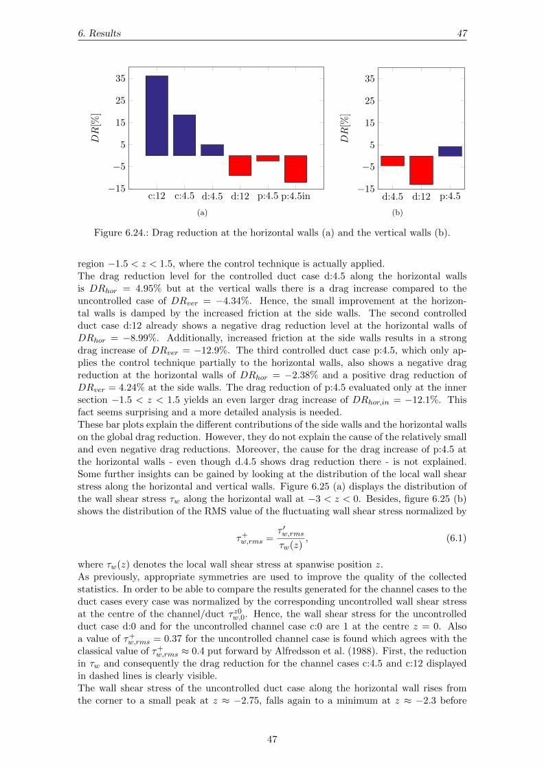
6. Results 47

c:12 c:4.5 d:4.5 d:12 p:4.5 p:4.5in−15

−5

5

15

25

35

DR

[%]

(a)

d:4.5 d:12 p:4.5−15

−5

5

15

25

35

DR

[%]

(b)

Figure 6.24.: Drag reduction at the horizontal walls (a) and the vertical walls (b).

region −1.5 < z < 1.5, where the control technique is actually applied.The drag reduction level for the controlled duct case d:4.5 along the horizontal wallsis DRhor = 4.95% but at the vertical walls there is a drag increase compared to theuncontrolled case of DRver = −4.34%. Hence, the small improvement at the horizon-tal walls is damped by the increased friction at the side walls. The second controlledduct case d:12 already shows a negative drag reduction level at the horizontal walls ofDRhor = −8.99%. Additionally, increased friction at the side walls results in a strongdrag increase of DRver = −12.9%. The third controlled duct case p:4.5, which only ap-plies the control technique partially to the horizontal walls, also shows a negative dragreduction at the horizontal walls of DRhor = −2.38% and a positive drag reduction ofDRver = 4.24% at the side walls. The drag reduction of p:4.5 evaluated only at the innersection −1.5 < z < 1.5 yields an even larger drag increase of DRhor,in = −12.1%. Thisfact seems surprising and a more detailed analysis is needed.These bar plots explain the different contributions of the side walls and the horizontal wallson the global drag reduction. However, they do not explain the cause of the relatively smalland even negative drag reductions. Moreover, the cause for the drag increase of p:4.5 atthe horizontal walls - even though d.4.5 shows drag reduction there - is not explained.Some further insights can be gained by looking at the distribution of the local wall shearstress along the horizontal and vertical walls. Figure 6.25 (a) displays the distribution ofthe wall shear stress τw along the horizontal wall at −3 < z < 0. Besides, figure 6.25 (b)shows the distribution of the RMS value of the fluctuating wall shear stress normalized by

τ+w,rms =

τ ′w,rmsτw(z)

, (6.1)

where τw(z) denotes the local wall shear stress at spanwise position z.As previously, appropriate symmetries are used to improve the quality of the collectedstatistics. In order to be able to compare the results generated for the channel cases to theduct cases every case was normalized by the corresponding uncontrolled wall shear stressat the centre of the channel/duct τ z0w,0. Hence, the wall shear stress for the uncontrolledduct case d:0 and for the uncontrolled channel case c:0 are 1 at the centre z = 0. Alsoa value of τ+

w,rms = 0.37 for the uncontrolled channel case is found which agrees with theclassical value of τ+

w,rms ≈ 0.4 put forward by Alfredsson et al. (1988). First, the reductionin τw and consequently the drag reduction for the channel cases c:4.5 and c:12 displayedin dashed lines is clearly visible.The wall shear stress of the uncontrolled duct case along the horizontal wall rises fromthe corner to a small peak at z ≈ −2.75, falls again to a minimum at z ≈ −2.3 before

47

6. Results 48

−3 −2 −1 00

1

2

z

τ w/τ

z0w,0

(a)

−3 −2 −1 00

0.5

1

1.5

z

τ+ w,rms

c:0c:12d:0d:4.5d:12p:4.5c:4.5

(b)

Figure 6.25.: Wall shear stress along the horizontal wall (a) and its RMS value (b).

it steadily rises to reach a constant level at −0.8 . z < 0. Its fluctuating value shows asignificant peak at the corner z = −3 but soon reaches the classical value of 0.4.The first peak of the controlled duct case d:4.5 is more pronounced than in d:0 and in-creased in magnitude. This peak is probably a result of the intensified streamwise vortexshown in figure 6.18 at the corner. This vortex convects high-speed fluid from the coreregion towards the corner, increasing the mean streamwise velocity close to the corner andconsequently the wall shear stress at this location. This effect can already be observed inthe 2D contour plot of the mean streamwise velocity in figure 6.2. Next to this peak, theexpected effect of the control technique can be found. In a long region at −2.3 . z < 0the wall shear stress is reduced compared to the uncontrolled case and is nearly constant.Thus, the average effect of the applied control technique is positive on the horizontal wallfor case d:4.5.At the centre of the duct the normalized wall shear stress of d:4.5 and c:4.5 are slightlydifferent maybe due to a too short averaging time or because of remaining effects of theside walls. The fluctuating wall shear stress τ+

w,rms is also reduced and agrees well withthe corresponding value for the controlled channel c4.5 at the centre of the duct.

For the controlled duct case d:12 the first peak is much more pronounced and its neg-ative effect on the averaged wall shear stress along the horizontal wall is unbalanced bythe reduction in the centre of the duct at −1.8 . z < 0. Besides, the reduction in thecentre of the duct is not nearly as good as for the corresponding channel case. This isprobably also caused by the effect of the side walls.The significant peak is probably formed by the strong streamwise vortex at the corneridentified for this case in figure 6.18. Another mechanism not present in the uncontrolledduct is the fluid being pushed against the side walls by the oscillating horizontal walls.Due to conservation of mass this fluid is deflected in wall normal direction as can be seenin figure 6.4 and maybe also in streamwise direction accelerating U . This could also con-tribute to the strong peak located at z ≈ −3 for the d:12 case.A reduction in τ+

w,rms for d:12 is visible in figure 6.25 (b) with a minimum at z ≈ −2agreeing with τ+

w,rms of the corresponding c:12 case. However, in the centre the fluctuatingwall shear stress for the d:12 case is again larger than that for the c:12 case.

The third controlled duct case p:4.5 also shows one significant peak the end of the con-trolled area z ≈ −1.5. Apart from that peak and the adjoining region the distributionof τw coincides with d:0 in the uncontrolled region close to the corner and with d:4.5 in

48

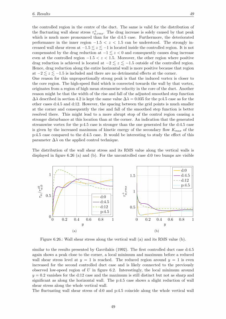
6. Results 49

the controlled region in the centre of the duct. The same is valid for the distribution ofthe fluctuating wall shear stress τ+

w,rms. The drag increase is solely caused by that peakwhich is much more pronounced than for the d:4.5 case. Furthermore, the deterioratedperformance in the inner region −1.5 < z < 1.5 can be understood. The strongly in-creased wall shear stress at −1.5 . z . −1 is located inside the controlled region. It is notcompensated by the drag reduction at −1 . z < 0 and consequently causes drag increaseeven at the controlled region −1.5 < z < 1.5. Moreover, the other region where positivedrag reduction is achieved is located at −2 . z . −1.5 outside of the controlled region.Hence, drag reduction along the entire horizontal wall is more positive because that regionat −2 . z . −1.5 is included and there are no detrimental effects at the corner.One reason for this unproportionally strong peak is that the induced vortex is closer tothe core region. The high-speed fluid which is convected towards the wall by that vortex,originates from a region of high mean streamwise velocity in the core of the duct. Anotherreason might be that the width of the rise and fall of the adjusted smoothed step function∆λ described in section 4.2 is kept the same value ∆λ = 0.035 for the p:4.5 case as for theother cases d:4.5 and d:12. However, the spacing between the grid points is much smallerat the corner and consequently the rise and fall of the smoothed step function is betterresolved there. This might lead to a more abrupt stop of the control region causing astronger disturbance at this location than at the corner. An indication that the generatedstreamwise vortex for the p:4.5 case is stronger than the one generated for the d:4.5 caseis given by the increased maximum of kinetic energy of the secondary flow Kmax of thep:4.5 case compared to the d:4.5 case. It would be interesting to study the effect of thisparameter ∆λ on the applied control technique.

The distribution of the wall shear stress and its RMS value along the vertical walls isdisplayed in figure 6.26 (a) and (b). For the uncontrolled case d:0 two bumps are visible

0 0.2 0.4 0.6 0.8 10

0.5

1

y

τ w/τ

z0w,0

d:0d:4.5d:12p:4.5

(a)

0 0.2 0.4 0.6 0.8 1

0.5

1

1.5

y

τ+ w,rms

d:0d:4.5d:12p:4.5

(b)

Figure 6.26.: Wall shear stress along the vertical wall (a) and its RMS value (b).

similar to the results presented by Gavrilakis (1992). The first controlled duct case d:4.5again shows a peak close to the corner, a local minimum and maximum before a reducedwall shear stress level at y = 1 is reached. The reduced region around y = 1 is evenincreased for the second controlled duct case and is likely connected to the previouslyobserved low-speed region of U in figure 6.2. Interestingly, the local minimum aroundy = 0.2 vanishes for the d:12 case and the maximum is still distinct but not as sharp andsignificant as along the horizontal wall. The p:4.5 case shows a slight reduction of wallshear stress along the whole vertical wall.The fluctuating wall shear stress of d:0 and p:4.5 coincide along the whole vertical wall

49

6. Results 50

and reach a value of τ+w,rms = 0.39 again close to the classical value of 0.4. Unlike the

behaviour along the horizontal wall the controlled cases d:4.5 and d:12 show an increasedτ+w,rms even at y = 1 caused by the disturbance of the moving walls.

50

7. Conclusion and Outlook

The effect of harmonic wall oscillation on drag reduction and on the secondary flow patternswere investigated via direct numerical simulations. To the best of the author’s knowledge,this is the first study where a flow control technique for turbulent drag reduction wastested in the duct geometry. However, a duct geometry is the natural choice for many lab-oratory experiments, with which DNS aims to compare. The present simulations allowedto address the discrepancy between numerical and experimental results observed by Gattiet al. (2015), the latter yielding less drag reduction. Besides, an investigation of the roleof the secondary motions, as a possible cause of this discrepancy, was conducted.In order to better understand the influence of different control parameters, four cases of theturbulent duct flow were simulated with the spectral element code Nek5000 (Fischer et al.,2008). One uncontrolled case was simulated and served as a reference. Two controlledcases, where both horizontal walls were almost completely oscillating were also simulated.They differ only in the chosen amplitude of wall velocity. In the third controlled duct caseonly the inner section of both horizontal walls was moved with the same amplitude of wallvelocity as the lower one of the two other controlled cases.The implementation was validated by comparing the results for one uncontrolled and onecontrolled channel case with data from the literature and data generated by a pseudo-spectral DNS code. The agreement between those was very good. Consequently, the ductflows are also considered to yield plausible results since they only differ in the appliedboundary conditions.

All cases consistently show that there is a strong interaction between the spanwise wallvelocity and the side walls, which can lead to severe detrimental effects. In some cases,in particular for the large spanwise oscillation amplitude, the effect of the side walls isnot confined to their vicinity but extends into the core of the flow. The drag reduction isobserved to be a local effect directly related to the local property of the spanwise Stokeslayer as the very good agreement between the mean streamwise velocity profiles at thecentre of the duct and in periodic channel flows show. However, this is only valid for smallamplitudes of wall velocity. Additionally, the effects of the side walls on the flow closeto them is clearly displayed in 2D contour plots. Mean wall-normal velocity and meanspanwise velocity show the formation of a strong streamwise vortex at the corner of theduct for the cases of almost completely moving walls, depicted in figure 7.1 (a). In the caseof partially applied control a new pair of counter rotating streamwise vortices is generatedat the lateral sides of the controlled region as depicted in figure 7.1 (b).

51

7. Conclusion and Outlook 52

z

y

(a)

z

y

(b)

Figure 7.1.: Schematic drawing of the induced streamwise vortices by the moving walls for(a) almost complete wall movement and (b) only inner section.

The RMS values of the fluctuating streamwise velocity show the expected reduction inthe centre of the duct. However, they are strongly amplified at the side walls and at thelateral sides of the controlled region for the first two and the third controlled case respec-tively. This indicates already that the overall effect of the applied control technique will beinferior to the results in the channel case. The same behaviour at the side walls and at theend of the controlled region is also found for the RMS of wall-normal velocity fluctuationsand the magnitude of the Reynolds stresses 〈u′v′〉, 〈u′w′〉, 〈v′w′〉.Investigation of the secondary flow yielded that the wall movement strengthens the sec-ondary flow, changes the shape of the classical pair of counter rotating streamwise vorticesand their location. The controlled cases applying almost complete wall movement amplifyone of the corner vortices which grows in size and pushes the other one closer to the centreof the duct. The new pair of counter rotating vortices for the third controlled case isclearly identified by streamline plots of the cross-stream motions.The achieved levels of drag reduction in the duct compared to the channel are poor. Onlythe case of almost complete wall movement and the lower amplitude of wall velocity yieldsa positive global drag reduction of 3% compared to 19% in the channel case. The othercontrolled cases even show an increase in global drag. Further insights are obtained bysplitting up the contributions of the horizontal walls and the vertical walls to the globaldrag reduction and by investigating the distribution of the wall shear stress along the hor-izontal and vertical walls. It is found that the region close to the corners and the regionaround the lateral sides of the controlled section are mainly responsible for the poor resultsregarding drag reduction in the current simulations of a turbulent duct flow.

The generated results raise new questions and further studies should be carried out tobetter understand the small or even negative achieved levels of drag reduction and theobserved change of the secondary flow. One possibly important parameter is the widthof the rise and fall of the implemented smoothed ”step” function, ∆λ, which was kept atone value for all the controlled duct cases in this thesis. This ”step” function was used tosmooth the transition between the uncontrolled and the controlled region of the horizontalwalls. A large difference between the peak in the wall shear stress distribution of the caseusing partially moving walls and the one with almost complete wall movement and thesame amplitude of wall velocity is found. This might be partially attributed due to a moreabrupt end of the controlled section because of fewer grid points to resolve the smoothedrise and fall of the ”step” function. Hence, a variation of this parameter and its impactson the flow would be interesting.Moreover, an investigation in a duct of higher aspect ratio, closer to the aspect ratio ofthe duct used in the experiment by Gatti et al. (2015), could help to clarify if there arestill perceptible effects of the interaction between the applied control technique and theside walls on the measured level of drag reduction in the centre of the duct. The currentresults already suggest that the wall shear stress distribution along the horizontal wall isconstant in a large region at the centre of the duct and almost as good as in the channel,

52

7. Conclusion and Outlook 53

at least for not too high amplitudes of wall velocity, W+m = 4.5. Furthermore, the available

results could be used to formulate the estimated effect of the applied control technique ondifferent combinations of aspect ratio and controlled region for W+

m = 4.5. Three assump-tions could lead to such a model to predict the achieved drag reduction: wall shear stressbeing the same as in the uncontrolled case above the steady part of the walls, a constantdrag increase at the end of the controlled section and a region of constant drag reductionabove the moving walls. Such a model should be tested against experimental results andcould be used to design further experimental investigations.Two other modifications of the setup could be of interest. First, investigation of the sec-ondary flow for a laminar controlled duct case could clarify the origin of the observedchanges in the secondary motions of a turbulent duct flow. The observed features in thecontrolled turbulent duct flow might be simply a result of the harmonic oscillation ofthe walls and their formation would be consequently completely different to the Reynoldsstress induced formation of the classical secondary motions in a duct. Finally, to bettermimic the actuator used by Gatti et al. (2015), which was limited in length and width,a limitation of the controlled region not only in spanwise but also in streamwise lengthcould be investigated.

53

Symbols and Abbreviations

Upper-case Roman

A stiffness matrixB channel/duct width, mass matrixC constant in log law, convection matrixCf skin friction coefficientD differentiation matrixE total number of elementsH channel/duct heightK kinetic energy of the secondary flow〈Kyz〉 K averaged over the whole cross section〈Kyz1〉 K averaged over the first window: y ∈ [0, 2] and z ∈ [−3,−2]Kn Knudsen numberL channel/duct lengthL space of Lebesgue-square-integrable functionsLN Legendre polynomial of order NP mean pressurePw mean pressure at the wallRe Reynolds numberReb Reynolds number based on bulk velocityReb,c Reynolds number based on bulk velocity of the centre planeRec Reynolds number based on centreline velocityReτ Reynolds number based on friction velocityS(x) smoothed ”step” functionUb bulk velocityUc centreline velocityUj j-component of the mean velocityWm amplitude of the wall velocityXN finite-dimensional trial spaceY N finite-dimensional test space

54

7. Conclusion and Outlook 55

Lower-case Roman

c convection velocityf body forceh channel/duct half heightp pressurep′ fluctuating pressuret timeu streamwise velocity, trial solution to Poisson equationuex exact solution to Poisson equationuj j-component of the instantaneous velocityu′j j-component of the fluctuating velocity

uτ friction velocityv wall-normal velocity, test functionw spanwise velocity, arbitrary solution within the trial space XN

0

x cartesian coordinate, streamwise directionxj j-component of cartesian coordinatey cartesian coordinate, wall-normal directionz cartesian coordinate, spanwise direction

Lower-case Greek

δij Kronecker deltaκ von Karman constantλ adjusted smoothed ”step” function∆λ width of rise and fall of adjusted smoothed ”step” functionρ densityµ dynamic viscosityν kinematic viscosityξ coordinate on reference elementσ stress tensorτ total shear stressτw wall shear stressω oscillation frequencyΩ whole problem domain

Ω reference element

Upper-case Greek

Π non-dimensional quantityΦ universal non-dimensional functionΩ mean streamwise vorticity

55

7. Conclusion and Outlook 56

Abbreviations

BDF3 third order backward differencingCFR constant flow rateCPG constant pressure gradientCPU central processing unitDNS direct numerical simulationDR drag reductionEXT3 third order extrapolationGLL Gauss–Lobatto LegendreNSE Navier–Stokes equationsPDE partial differential equationRANS Reynolds-averaged-Navier–StokesRMS root-mean-squareSEM Spectral Element Method

56

List of Figures

2.1. Schematic drawing of (a) duct and (b) channel flow. . . . . . . . . . . . . . 8

2.2. Sketch of Stokes’ second problem. . . . . . . . . . . . . . . . . . . . . . . . . 12

2.3. Solutions to Stokes’ second problem. . . . . . . . . . . . . . . . . . . . . . . 13

3.1. Example of Lagrange interpolants for the Legendre spectral element basisfunctions on the reference element corresponding to N = 5. . . . . . . . . . 18

4.1. Schematic drawing of controlled channel flow. . . . . . . . . . . . . . . . . . 23

4.2. Schematic drawing of (a) controlled duct cases 1 and 2 and (b) case 3. . . . 25

4.3. The smoothed step function applied to a region close to z = −3. . . . . . . 26

5.1. Mean streamwise velocity u+ (a) and Reynolds stress 〈u′v′〉/u2τ (b) in the

uncontrolled channel. . . . . . . . . . . . . . . . . . . . . . . . . . . . . . . . 28

5.2. RMS values in the uncontrolled channel. . . . . . . . . . . . . . . . . . . . . 28

5.3. Mean streamwise velocity u+ (a) and Reynolds stress 〈u′v′〉/u2τ (b) in the

uncontrolled and controlled channel. . . . . . . . . . . . . . . . . . . . . . . 29

5.4. RMS of streamwise u+rms (a) and wall-normal v+

rms (b) velocity fluctuationsin the uncontrolled and controlled channel. . . . . . . . . . . . . . . . . . . 30

5.5. RMS of spanwise velocity fluctuations w+rms in the uncontrolled and con-

trolled channel. . . . . . . . . . . . . . . . . . . . . . . . . . . . . . . . . . . 30

6.1. Sketch of partitioning of 2D contour plots. . . . . . . . . . . . . . . . . . . . 31

6.2. Mean streamwise velocity of the four duct cases. . . . . . . . . . . . . . . . 32

6.3. Inner scaled mean streamwise velocity at z = 0 (a) and at z = −2.5 (b). . . 33

6.4. Mean wall-normal velocity of the four duct cases. . . . . . . . . . . . . . . . 33

6.5. Mean spanwise velocity of the four duct cases. . . . . . . . . . . . . . . . . . 34

6.6. Inner scaled mean wall-normal velocity (a) and mean spanwise velocity (b)at z = −2.5. . . . . . . . . . . . . . . . . . . . . . . . . . . . . . . . . . . . . 35

6.7. RMS of streamwise velocity fluctuations of the four duct cases. . . . . . . . 36

6.8. Inner scaled RMS of fluctuating streamwise velocity at z = 0 (a) and atz = −2.5 (b). . . . . . . . . . . . . . . . . . . . . . . . . . . . . . . . . . . . 36

6.9. RMS of wall-normal velocity fluctuations of the four duct cases. . . . . . . . 37

6.10. Inner scaled RMS of fluctuating wall-normal velocity at z = 0 (a) and atz = −2.5 (b). . . . . . . . . . . . . . . . . . . . . . . . . . . . . . . . . . . . 37

6.11. RMS of spanwise velocity fluctuations of the four duct cases. . . . . . . . . 38

6.12. Inner scaled RMS of fluctuating spanwise velocity at z = 0 (a) and atz = −2.5 (b). . . . . . . . . . . . . . . . . . . . . . . . . . . . . . . . . . . . 38

6.13. Reynolds stress 〈u′v′〉 of the four duct cases. . . . . . . . . . . . . . . . . . . 39

6.14. Reynolds stress 〈u′v′〉/u2τ at z = 0 (a) and at z = −2.5 (b). . . . . . . . . . 39

6.15. Reynolds stress 〈u′w′〉 of the four duct cases. . . . . . . . . . . . . . . . . . 40

6.16. Reynolds stress 〈u′w′〉/u2τ at z = −2.5. . . . . . . . . . . . . . . . . . . . . . 40

6.17. Reynolds stress 〈v′w′〉 of the four duct cases. . . . . . . . . . . . . . . . . . 41

57

List of Figures 58

6.18. Secondary flow field of all four duct cases using the same scaling for stream-lines and contour plot. . . . . . . . . . . . . . . . . . . . . . . . . . . . . . . 42

6.19. Kinetic energy of the secondary flow K of the uncontrolled duct case d:0. . 436.20. Secondary flow field of the controlled duct case d:4.5. . . . . . . . . . . . . . 436.21. Secondary flow field of the controlled duct case d:12. . . . . . . . . . . . . . 446.22. Secondary flow field of the controlled duct case p:4.5. . . . . . . . . . . . . . 456.23. Global drag reduction for each controlled case. . . . . . . . . . . . . . . . . 466.24. Drag reduction at the horizontal walls (a) and the vertical walls (b). . . . . 476.25. Wall shear stress along the horizontal wall (a) and its RMS value (b). . . . 486.26. Wall shear stress along the vertical wall (a) and its RMS value (b). . . . . . 49

7.1. Schematic drawing of the induced streamwise vortices by the moving wallsfor (a) almost complete wall movement and (b) only inner section. . . . . . 52

58

List of Tables

4.1. Comparison of geometrical parameters, resolution and Reynolds numberbetween channel and duct reference cases. . . . . . . . . . . . . . . . . . . . 25

4.2. Different control parameters for channel and duct cases. . . . . . . . . . . . 26

5.1. Comparison of some mean flow variables between the present thesis and theresults from Kim et al. (1987). . . . . . . . . . . . . . . . . . . . . . . . . . 27

6.1. Comparison of scalar values of the kinetic energy of the secondary flow field. 436.2. Comparison of wall shear stress related scalars between all investigated cases. 46

59

Bibliography

P. H. Alfredsson, A. V. Johansson, J. H. Haritonidis, and H. Eckelman. The fluctuatingwall-shear stress and the velocity field in the viscous sublayer. Physics of Fluids, 31(5):1026–1033, 1988.

A. Baron and M. Quadrio. Turbulent drag reduction by spanwise wall oscillations. AppliedScientific Research, 55:311–326, 1995.

D. Bechert, M. Bruse, W. Hage, J. v. d. Hoeven, and G. Hoppe. Experiments on drag-reducing surfaces and their optimization with an adjustable geometry. Journal of FluidMechanics, 338:59–87, 1997.

J.-I. Choi and H. J. Xu, C.-X.and Sung. Drag reduction by spanwise wall oscillation inwall-bounded turbulent flows. AIAA Journal, 40(5):842–850, 2002.

K. Choi. Near-wall structure of turbulent boundary layer with spanwise-wall oscillation.Physics of Fluids, 14(7):2530–2542, 2002.

K.-S. Choi, J.-R. DeBisschop, and B. R. Clayton. Turbulent boundary-layer control bymeans of spanwise-wall oscillation. American Institute of Aeronautics and Astronoutics,36(7):1157–1163, 1998.

G. N. Coleman and R. D. Sandberg. A primer on direct numerical simulation of turbu-lence - methods, procedures and guidelines. Technical report, Aerodynamics & FlightMechanics Research Group, School of Engineering Sciences, University of Southampton,2010.

S. Corrsin. Turbulent flow. American Scientist, 49(3):300–325, 1961.

W. Couzy. Spectral element discretization of the unsteady Navier–Stokes equations and itsiterative solution on parallel computers. PhD thesis, Ecole Polytechnique Federale deLaussane, 1995.

M. O. Deville, P. F. Fischer, and E. H. Mund. High-Order Methods for IncompressibleFluid Flow. Cambridge University Press, 2002. ISBN 9780511546792.

P. F. Fischer, J. W. Lottes, and S. G. Kerkemeier. Nek5000: Open source spectral elementCFD solver. available at http://nek5000.mcs.anl.gov, 2008.

J. Fish and T. Belytschko. A First Course in Finite Elements. John Wiley & Sons, Ltd,2007.

K. Fukagata, K. Iwamoto, and N. Kasagi. Contribution of Reynolds stress distribution tothe skin friction in wall-bounded flows. Physics of Fluids, 14(11):L73–76, 2002.

M. Gad-el Hak. Flow Control – Passive, Active and Reactive Flow Management. Cam-bridge University Press, Cambridge, 2000.

R. Garcia-Mayoral and J. Jimenez. Drag reduction by riblets. Philosophical Transactionsof the Royal Society A, 369:1412–1427, 2011.

60

Bibliography 61

D. Gatti, A. Guttler, B. Frohnapfel, and C. Tropea. Experimental assessment of spanwise-oscillating dielectric electroactive surfaces for turbulent drag reduction in an air channelflow. Experiments in Fluids, 56(5), 2015.

S. Gavrilakis. Numerical simulation of low-Reynolds-number turbulent flow through astraight square duct. Journal of Fluid Mechanics, 244:101–129, 1992.

F. Gessner and J. B. Jones. On some aspects of fully-developed turbulent flow in rectan-gular channels. Journal of Fluid Mechanics, 23:689–713, 1965.

D. Gottlieb and S. Orszag. Numerical Analyses of Spectral Methods: Theory and Applica-tion. SIAM-CBMS, Philadelphia, 1977.

W. Jung, N. Mangiavacchi, and R. Akhavan. Suppression of turbulence in wall-boundedflow by high-frequency spanwise oscillations. Physics of Fluids, 4:1605–1607, 1992.

J. Kim. Physics and control of wall turbulence for drag reduction. Philosophical Trans-actions of the Royal Society of London A: Mathematical, Physical and Engineering Sci-ences, 369:1396–1411, 2011.

J. Kim, P. Moin, and R. Moser. Turbulence statistics in fully developed channel flow atlow Reynolds number. Journal of Fluid Mechanics, 177:133–166, 1987.

P. Kundu, I. Cohen, and R. Dowling. Fluid Mechanics. Elsevier, 5 edition, 2012.

F. Laadhari, L. Skandaji, and R. Morel. Turbulence reduction in a boundary layer by alocal spanwise oscillating surface. Physics of Fluids, 6:3218–3220, 1994.

S. Lardeau and M. A. Leschziner. The streamwise drag-reduction response of a boundarylayer subjected to a sudden imposition of transverse oscillatory wall motion. Physics ofFluids, 25(075109), 2013.

P. Luchini and M. Quadrio. A low-cost parallel implementation of direct numerical simu-lation of wall turbulence. Journal of Computational Physics, 211:551–571, 2006.

J. Malm, P. Schlatter, P. F. Fischer, and D. Henningson. Stabilization of the spectralelement method in convection dominated flows by recovery of skew-symmetry. Journalof Scientific Computing, 57:254–277, 2013.

R. D. Moser, J. Kim, and N. N. Mansour. Direct numerical simulation of turbulent channelflow up to Reτ = 590. Physics of Fluids, 11(4):943–945, 1999.

H. Oertel jr., editor. Prandtl - Fuhrer durch die Stroemungslehre. Springer Vieweg, 10thedition, 2012.

R. Orlu and P. Schlatter. Comparison of experiments and simulations for zero pressuregradient turbulent boundary layers at moderate Reynolds numbers. Experiments inFluids, 54(6), 2013.

R. L. Panton. Incompressible Flow. John Wiley & Sons, Inc., Hoboken, New Jersey, 4thedition, 2013.

A. Patera. A spectral element method for fluid dynamics: Laminar flow in a channelexpansion. Journal of Computational Physics, 54:468–588, 1984.

S. B. Pope. Turbulent Flows. Cambridge University Press, 7 edition, 2010.

L. Prandtl. Uber die ausgebildete Turbulenz. In Verh. 2nd Intl Kong, NACA Tech. Memo62, 2nd Intl. Kong fur Tech. Mech., page 435, Zurich, 1926.

M. Quadrio. Drag reduction in turbulent boundary layer by in-plane wall motion. Philo-sophical Transactions of the Royal Society of London A: Mathematical, Physical andEngineering Sciences, 369(1940):1428–1442, 2011.

61

Bibliography 62

M. Quadrio and P. Ricco. Critical assessment of turbulent drag reduction through spanwisewall oscillations. Journal of Fluid Mechanics, 521:251–271, 2004.

P. Ricco, C. Ottonelli, Y. Hasegawa, and M. Quadrio. Changes in turbulent dissipation ina channel flow with oscillating walls. Journal of Fluid Mechanics, 700:77–104, 2012.

P. Schlatter and R. Orlu. Turbulent boundary layers at moderate Reynolds number: inflowlength and tripping effects. Journal of Fluid Mechanics, 710:5–34, 2012.

H. Schlichting and K. Gersten. Grenzschicht-Theorie. Springer Berlin Heidelberg, 10edition, 2006.

M. Skote. Turbulent boundary layer flow subject to streamwise oscillation of spanwisewall-velocity. Physics of Fluids, 23(081703), 2011.

J. H. Spurk. Stromungslehre : Einfuhrung in die Theorie der Stromungen. Springer BerlinHeidelberg, 8th edition, 2010.

H. Tennekes and J. L. Lumley. A First Course in Turbulence. MIT Pres, 1972.

E. Touber and M. A. Leschziner. Near-wall streak modification by spanwise oscillatorywall motion and drag-reduction mechanisms. Journal of Fluid Mechanics, 693:150–200,2012.

R. Vinuesa, A. Noorani, A. Lozano-Duran, G. K. El Khoury, P. Schlatter, P. F. Fischer,and H. M. Nagib. Aspect ratio effects in turbulent duct flows studied through directnumerical simulation. Journal of Turbulence, 15(10):677–706, 2014.

R. Vinuesa, P. Schlatter, and H. M. Nagib. Characterization of the secondary flow inturbulent rectangular ducts with varying aspect ratio. In International Symposiom OnTurbulence and Shear Flow Phenomena, 2015.

P. R. Viswanath. Aircraft viscous drag reduction using riblets. Progress in AerospaceSciences, 38:571–600, 2002.

A. Yakeno, Y. Hasegawa, and N. Kasagi. Modification of quasi-streamwise vortical struc-ture in a drag-reduced turbulent channel flow with spanwise wall oscillation. Physics ofFluids, 26(085109):–, 2014.

J. Zierep and K. Buhler. Grundzuge der Stromungslehre. Springer Fachmedien Wiesbaden,13 edition, 2013.

62

Appendix

The Appendix is used for some of the more complicated derivations which are not necessaryto understand the main part.

A. Best fit property

In order to show that the trial solution u(x) is the best one among all functions in thetrial space XN

0 , an energy inner product and its induced norm are defined.

a(u, v) :=

∫Ω

du

dx

dv

dxdx =

∫Ω

(u)′(v)′dx, ∀u, v ∈ H10 (7.1)

||v||a :=√a(v, v), ∀u, v ∈ H1

0 (7.2)

In this context the (·)′ denotes the first derivative.With these definitions it will be shown that the deviation between the exact solution uexand an arbitrary solution w within the trial space XN

0 is greater or equal to the deviationbetween the exact solution and the approximate solution u (in terms of the previouslydefined norm). That is

||w − uex||a ≥ ||u− uex||a, ∀w ∈ XN0 . (7.3)

This can be shown by substituting v = w − u ∈ XN0 into the left-hand side and using the

definition of the norm 7.2 above

||w − uex||2a = ||(v + u)− uex||2a (7.4)

= ||v + (u− uex)||2a (7.5)

=

∫Ω

(v + (u− uex))′(v + (u− uex))′dx (7.6)

=

∫Ω

(v)′2 + 2(v)′(u− uex)′ + (u− uex)′2dx (7.7)

=

∫Ω

(v′)2 + (u− uex)′2dx (7.8)

≥∫

Ω(u− uex)′2dx = ||u− uex||2a. (7.9)

The second term in 7.7 vanishes because∫Ω

(v)′(u− uex)′dx =

∫Ω

(v)′(u)′ − (v)′(uex)′dx (7.10)

=

∫Ω

(v)′(u)′dx−[v(uex)′

]∂Ω

+

∫Ωv(u)′′dx (7.11)

=

∫Ω

(v)′(u)′ −∫

Ωvfdx (7.12)

= 0, ∀v ∈ XN0 (7.13)

The fact that v vanishes at the boundaries ∂Ω is used as well as the model problem 3.1and its weak form 3.9.

63

7. Appendix 64

B. Lagrangian interpolants

For a set of N + 1 distinct points ξi Lagrangian basis polynomials φj(ξ) are constructedso that they are zero for all of the distinct points except one of the points. At this onepoint, their value is 1. More precisely, they satisfy the condition

φj(ξi) = δij , 0 ≤ i, j ≤ N, ξ ∈ Ω. (7.14)

Lagrangian basis polynomials can be written in a compact form as

φj(ξ) :=N∏i=0i 6=j

ξ − ξiξj − ξi

, 0 ≤ j ≤ N, ξ ∈ Ω. (7.15)

This formula can be easily understood because the numerator vanishes for all ξ = ξi exceptfor ξ = ξj . For the latter case the result is one because the numerator and denominatorare the same so the Kronecker delta condition 7.14 is satisfied. An equivalent form ofequation 7.15 is given by

φj(ξ) =

N∏i=0

(ξ − ξi)

(ξ − ξj)N∏i=0i 6=j

(ξj − ξi), 0 ≤ j ≤ N, ξ ∈ Ω. (7.16)

So the numerator is the polynomial of degree N with roots in ξi. The Gauss–Lobatto–Legendre (GLL) quadrature points are defined by

(1− ξ2)L′N (ξ) = 0 =N∏i=0

(ξ − ξi), ∀ξ ∈ Ω, (7.17)

where L′N (ξ) is the first derivative of the Legendre polynomial LN of order N and ξi arethe GLL points. Therefore, the numerator of equation 7.16 is simply (1− ξ2)L′N (ξ).The first derivative of a polynomial l(ξ) of degree N at one of its roots ξj can be given by

l(ξ) =N∏i=0

(ξ − ξi) (7.18)

l′(ξj) =N∏i=0i 6=j

(ξj − ξi), 0 ≤ j ≤ N, (7.19)

which can be easily shown by using the product rule.One part of the denominator in equation 7.16 is therefore identified as the first derivativeof the numerator at one of its roots. The first derivative of the left-hand side of equation7.17 is given by the definiton of the Legendre polynomials

− d

dx

((1− x2)

d

dxLN (x)

)= N(N + 1)LN (x), N = 0, 1, .... (7.20)

Therefore, the denominator in equation 7.16 is [−N(N + 1)LN (ξj)](ξ − ξj) and the La-grangian interpolation polynomial of the Gauss-Lobatto-Legendre quadrature points isgiven by

φj(ξ) =−1

N(N + 1)

(1− ξ2)L′N (ξ)

(ξ − ξj)LN (ξj), 0 ≤ j ≤ N, ξ ∈ Ω. (7.21)

64