Embed Size (px)
Citation preview
Direct Strength Method (DSM) Design Guide DESIGN GUIDE CFXX-X January, 2006 Committee on Specifications for the Design of Cold-Formed Steel Structural Members American Iron and Steel Institute
i
Preface The Direct Strength Method is an entirely new design method for cold-formed steel. Adopted in 2004 as Appendix 1 to the North American Specification for the Design of Cold-Formed Steel Structural Members, this Guide provides practical and detailed advice on the use of this new and powerful design method. Features of the Guide include Design examples: Extensive design examples, with thorough commentary, covering 14 different cold-formed steel cross-sections under a variety of different loading and boundary conditions are provided (Chapter 8). The bulk of the design examples are based on the AISI (2002) Cold-Formed Steel Design Manual and allow engineers to make direct comparison between the Direct Strength Method and conventional design. Tutorial: Introductory material to help engineers interpret elastic buckling analysis results, the heart of the Direct Strength Method, is provided (e.g., see Figure 2). Charts: Prescriptive guidelines (Chapter 4) and an example (Section 8.13) for developing beam charts using the Direct Strength Method are provided. Similar examples are given for column charts – together they can be used to create span and load tables based on the Direct Strength Method. The finer points: Details are not skipped over, for example, extensive discussion on how to handle unique situations in the elastic buckling analysis of members is provided (Section 3.3).
Acknowledgments
Funding for the development of this Guide was provided to Ben Schafer at Johns Hopkins University by the American Iron and Steel Institute. Members and friends of the American Iron and Steel Institute Committee on Specifications for the Design of Cold-Formed Steel Structural Members. provided useful feedback in the development of this Guide. In particular, Helen Chen, Bob Glauz, Perry Green, Dick Kaehler, and Tom Miller provided comments that greatly improved the final version.

ii
Mnl 94 kip in⋅=
(Eq. 1.2.2-5)(Eq. 1.2.2-6)
Mnl Mne λl 0.776≤if
1 0.15Mcrl
Mne
0.4
⋅−
Mcrl
Mne
0.4
Mne⋅
λl 0.776>if
:=
(Eq. 1.2.2-7)(subscript "l" = "l")λl 1.22=λlMne
Mcrl:=
Local buckling check per DSM 1.2.2.2
(fully braced)Mne 127 kip in⋅=Mne My:=
per DSM 1.2.2, Mn is the minimum of Mne, Mnl, Mnd. For a fully braced member lateral-torsional buckling will not occur and thus Mne = My, Mnl and Mnd must still be checked.
Mcrd 108 kip in⋅=Mcrd 0.85 My⋅:=
Mcrl 85 kip in⋅=Mcrl 0.67 My⋅:=
My 126.55 kip⋅ in⋅:=
Inputs from the finite strip analysis include:
Finite strip analysis of 9CS2.5x059 in pure bending as summarized in Example 3.2.1
Determination of the bending capacity for a fully braced member is equivalent to determining the effective section modulus at yield in the main Specification. see AISI (2002) example I-8.
8.1-1 Computation of bending capacity for a fully braced member (AISI 2002 Example I-8)
Given: a. Steel: Fy = 55 ksib. Section 9CS2.5x059 as shown to the rightc. Finite strip analysis results (Section 3.2.1)Required:1. Bending capacity for fully braced member2. Bending capacity at L=56.2 in. (AISI 2002 Example II-1)3. Effective moment of inertia4. Compression capacity for a fully braced member5. Compression capacity at a uniform compressive stress of 37.25 ksi (AISI 2002 Example III-1)6. Beam-column design (AISI 2002 Example III-1)
8.1 C-section with lips
Design Examples Quick Start
Mn
Ω b56 kip in⋅=Ω b 1.67:=ASD:
φb Mn⋅ 84 kip in⋅=φb 0.9:=LRFD:
The geometry of this section falls within the "pre-qualified" beams of DSM 1.1.1.2 and the higher φ and lower Ω of DSM Section 1.2.2 may therefore be used.
Mn 93 kip in⋅=Mn min Mne Mnl Mnd( )( ):=
Predicted bending capacity per 1.3
Mnd 93 kip in⋅=
(Eq. 1.2.2-8)(Eq. 1.2.2-9)
Mnd My λd 0.673≤if
1 0.22Mcrd
My
0.5
⋅−
Mcrd
My
0.5
My⋅
λd 0.673>if
:=
(Eq. 1.2.2-10)λd 1.08=λdMy
Mcrd:=
Distortional buckling check per DSM 1.2.2.3
“:=” vs. “=” ?“:=” in Mathcad this “:=” symbol is
how equations are defined. The right hand side is evaluated and the
answer assigned to the left hand side. In this example Mcrl is defined
as 0.67My and then evaluated.
“=” in Mathcad the “=” symbol is simply a print statement. In this
example Mcrl is defined as 0.67Mywith the “:=” symbol and its value,
85 kip-in., is printed to the screen with the “=” symbol.
“|” in Mathcad the “|” symbol is for if-then statements. In this example if λl < 0.776 Mnl is Mne, otherwise if λl
> 0.776 then the second expression applies. The vertical bar shows the
potential choices for Mnl.
if-then statements
“min” in Mathcad the “min”function operates on variables in a
row vector, and in this case provides the member strength Mn.
min
In Mathcad the solution includes units. Since My is given units of kip-
in. and Mcrd is defined in terms of My, Mnd is also in kip-in. In the
program units can be changed and the results will modify accordingly.
units
Equation numbers refer to the relevant parts of DSM (Appendix 1 AISI 2004)
This lists the six design examples provided in Section 8.1. Each design example uses the same cross-section,
in this case, C-section 9CS2.5x059. Reference to AISI (2002) Design
Manual examples are also provided.
Design examples provided in Chapter 8.
iii
Symbols and definitions Unless explicitly defined herein, variables referred to in this Guide are defined in the Specification (AISI 2001, 2004) or the Design Manual (AISI 2002). An abbreviated list of variables is provided here for the reader’s convenience. Mcrl Critical elastic local buckling moment determined in accordance
with Appendix 1 (DSM) Section 1.1.2
Mcrd Critical elastic distortional buckling moment determined in accordance with Appendix 1 (DSM) Section 1.1.2
Mcre Critical elastic lateral-torsional bucking moment determined in accordance with Appendix 1 (DSM) Section 1.1.2
Mnl Nominal flexural strength for local buckling determined in accordance with Appendix 1 (DSM) Section 1.2.2.2
Mnd Nominal flexural strength for distortional buckling determined in accordance with Appendix 1 (DSM) Section 1.2.2.3
Mne Nominal flexural strength for lateral-torsional buckling determined in accordance with Appendix 1 (DSM) Section 1.2.2.1
Mn Nominal flexural strength, Mn, is the minimum of Mne, Mnl and Mnd
My Yield moment (SgFy)
Pcrl Critical elastic local column buckling load determined in accordance with Appendix 1 (DSM) Section 1.1.2
Pcrd Critical elastic distortional column buckling load determined in accordance with Appendix 1 (DSM) Section 1.1.2
Pcre Minimum of the critical elastic column buckling load in flexural, torsional, or torsional-flexural buckling determined in accordance with Appendix 1 (DSM) Section 1.1.2
Pnl Nominal axial strength for local buckling determined in accordance with Appendix 1 (DSM) Section 1.2.1.2
Pnd Nominal axial strength for distortional buckling determined in accordance with Appendix 1 (DSM) Section 1.2.1.3
Pne Nominal axial strength for flexural, torsional, or torsional- flexural buckling determined in accordance with Appendix 1 (DSM) Section 1.2.1.1
Pn Nominal axial strength, Pn, is the minimum of Pne, Pnl and Pnd
Py Squash load (AgFy)
iv
Terms Unless explicitly defined herein, terms referred to in this Guide are defined in the Specification (AISI 2001, 2004). An abbreviated list of terms is provided here for the reader’s convenience. Elastic buckling value. The load (or moment) at which the equilibrium of the member is neutral
between two alternative states: the buckled shape and the original deformed shape.
Local buckling. Buckling that involves significant distortion of the cross-section, but this distortion includes only rotation, not translation, at the internal fold lines (e.g., the corners) of a member. The half-wavelength of the local buckling mode should be less than or equal to the largest dimension of the member under compressive stress.
Distortional buckling. Buckling that involves significant distortion of the cross-section, but this distortion includes rotation and translation at one or more internal fold lines of a member. The half-wavelength is load and geometry dependent, and falls between local and global buckling.
Global buckling. Buckling that does not involve distortion of the cross-section, instead translation (flexure) and/or rotation (torsion) of the entire cross-section occurs. Global, or “Euler” buckling modes: flexural, torsional, torsional-flexural for columns, lateral-torsional for beams, occur as the minimum mode at long half-wavelengths.
Fully braced. A cross-section that is braced such that global buckling is restrained.
Related Definitions from the North American Specification for the Design of Cold-Formed Steel Structural Members (AISI 2001)
Local Buckling. Buckling of elements only within a section, where the line junctions between elements remain straight and angles between elements do not change.
Distortional Buckling. A mode of buckling involving change in cross-sectional shape, excluding local buckling.
Torsional-Flexural Buckling. Buckling mode in which compression members bend and twist simultaneously without change in cross-sectional shape.
Allowable Design Strength. Allowable strength, Rn/Ω, (force, moment, as appropriate), provided by the structural component.
Design Strength. Factored resistance, φRn (force, moment, as appropriate), provided by the structural component.
Nominal Strength. The capacity Rn of a structure or component to resist effects of loads, as determined in accordance with this Specification using specified material strengths and dimensions.
Required Allowable Strength. Load effect (force, moment, as appropriate) acting on the structural component determined by structural analysis from the nominal loads for ASD (using all appropriate load combinations).
Required Strength. Load effect (force, moment, as appropriate) acting on the structural component determined by structural analysis from the factored loads for LRFD (using all appropriate load combinations).

v
Table of Contents
1 Introduction .......................................................................................................1 1.1 Using this Design Guide… ............................................................................................. 1 1.2 Why use DSM (Appendix 1) instead of the main Specification? ................................... 2 1.3 Designing with DSM (Appendix 1) and the main Specification .................................... 2
1.3.1 Approved usage, Mn and Pn .................................................................................... 3 1.3.2 Pre-qualified members ............................................................................................ 4 1.3.3 Rational analysis ..................................................................................................... 5
1.4 Limitations of DSM: practical and theoretical................................................................ 6
2 Elastic buckling: Pcrl, Pcrd, Pcre, Mcrl, Mcrd, Mcre .............................................7 2.1 Local, Distortional, and Global Buckling ....................................................................... 8 2.2 Elastic buckling upperbounds ......................................................................................... 9 2.3 Finite strip solutions...................................................................................................... 10
2.3.1 CUFSM and other software .................................................................................. 10 2.3.2 Interpreting a solution ........................................................................................... 11 2.3.3 Ensuring an accurate solution ............................................................................... 13 2.3.4 Programming classical finite strip analysis........................................................... 13
2.4 Finite element solutions ................................................................................................ 14 2.5 Generalized Beam Theory ............................................................................................ 15 2.6 Manual elastic buckling solutions................................................................................. 15
3 Member elastic buckling examples by the finite strip method ...................16 3.1 Construction of finite strip models ............................................................................... 16 3.2 Example cross-sections................................................................................................. 16
3.2.1 C-section with lips ................................................................................................ 17 3.2.2 C-section with lips modified ................................................................................. 19 3.2.3 C-section without lips (track section) ................................................................... 21 3.2.4 C-section without lips (track) modified................................................................. 24 3.2.5 Z-section with lips................................................................................................. 26 3.2.6 Z-section with lips modified.................................................................................. 28 3.2.7 Equal leg angle with lips....................................................................................... 30 3.2.8 Equal leg angle...................................................................................................... 32 3.2.9 Hat section ............................................................................................................ 34 3.2.10 Wall panel section................................................................................................. 36 3.2.11 Rack post section .................................................................................................. 38 3.2.12 Sigma section ........................................................................................................ 40
3.3 Overcoming difficulties with elastic buckling determination in FSM.......................... 42 3.3.1 Indistinct local mode............................................................................................. 42 3.3.2 Indistinct distortional mode .................................................................................. 43 3.3.3 Multiple local or distortional modes (stiffeners) .................................................. 46 3.3.4 Global modes at short unbraced lengths ............................................................... 47
vi
3.3.5 Global modes with different bracing conditions................................................... 48 3.3.6 Influence of moment gradient............................................................................... 49 3.3.7 Partially restrained modes..................................................................................... 50 3.3.8 Boundary conditions for repeated members ......................................................... 51 3.3.9 Members with holes.............................................................................................. 52 3.3.10 Boundary conditions at the supports not pinned................................................... 53 3.3.11 Built-up cross-sections.......................................................................................... 54
4 Beam design .....................................................................................................56 4.1 Beam design for fully braced beams............................................................................. 56 4.2 Beam charts, local, distortional, and global buckling as a function of length .............. 57 4.3 Deflections and serviceability....................................................................................... 59 4.4 Combining DSM and the main Specification for beams .............................................. 60
4.4.1 Shear ..................................................................................................................... 60 4.4.2 Combined bending and shear................................................................................ 60 4.4.3 Web crippling........................................................................................................ 60
4.5 Notes on example problems from AISI (2002) Design Manual ................................... 61
5 Column design .................................................................................................62 5.1 Column design for continuously braced columns......................................................... 62 5.2 Creating column charts ................................................................................................. 63 5.3 Notes on example problems from the 2002 AISI Manual ............................................ 65
6 Beam-column design .......................................................................................66 6.1 Main Specification methodology .................................................................................. 66 6.2 Design examples ........................................................................................................... 67 6.3 Future directions for DSM: Direct analysis of beam-columns ..................................... 68
6.3.1 Direct analysis beam-column design strength example........................................ 68
7 Product development ......................................................................................73 7.1 Cross-section optimization............................................................................................ 73 7.2 Developing span and load tables................................................................................... 73 7.3 Rational analysis vs. chapter F testing.......................................................................... 74 7.4 New pre-qualified members and extending the bounds of a pre-qualified member.... 75
8 Design examples ..............................................................................................77 8.1 C-section with lips ........................................................................................................ 78
8.1.1 Flexural strength for a fully braced member (AISI 2002 Example I-8) 8.1.2 Flexural strength for L=56.2 in. (AISI 2002 Example II-1) 8.1.3 Effective moment of inertia (AISI 2002 Example I-8) 8.1.4 Compressive strength for a continuously braced column (AISI 2002 Example I-8) 8.1.5 Compressive strength at Fn=37.25 ksi (AISI 2002 Example III-1)
vii
8.1.6 Beam-column design strength (AISI 2002 Example III-1) 8.2 C-section with lips modified ......................................................................................... 89
8.2.1 Flexural strength for a fully braced member 8.2.2 Compressive strength for a continuously braced column 8.2.3 Compressive strength at Fn=37.25 ksi
8.3 C-section without lips (track section) ........................................................................... 93 8.3.1 Flexural strength about strong axis for a fully braced … (AISI 2002 Example I-9) 8.3.2 Flexural strength at Fc=30.93 ksi (AISI 2002 Example II-3) 8.3.3 Compressive strength for a continuously braced column 8.3.4 Compressive strength for L=49.3 in. 8.3.5 Flexural strength about weak-axis (flange tips in compression) for L=49.3 in. 8.3.6 Beam-column design strength for L=49.3 in., & Pu = 2.8 kip & Mu = 0.32 kip-in.
8.4 C-section without lips modified (track section) .......................................................... 101 8.4.1 Flexural strength about strong axis for a fully braced member 8.4.2 Compressive strength for a continuously braced column
8.5 Z-section with lips....................................................................................................... 103 8.5.1 Flexural strength for a fully braced member 8.5.2 Flexural strength for L=48.5 in. (AISI 2002 Example II-2) 8.5.3 Compressive strength for a continuously braced column 8.5.4 Compressive strength at Fn=25.9 ksi (AISI 2002 Example III-6)
8.6 Z-section with lips modified........................................................................................ 109 8.6.1 Flexural strength for a fully braced member 8.6.2 Compressive strength for a continuously braced column 8.6.3 Compressive strength at Fn=25.9 ksi
8.7 Equal leg angle with lips............................................................................................. 113 8.7.1 Flexural strength about x-axis for a fully braced member 8.7.2 Flexural strength about minimum principal axis for L=18 in. (AISI 2002 III-4) 8.7.3 Compressive strength for a continuously braced column 8.7.4 Compressive strength at Fn=14.7 ksi (AISI 2002 Example III-4) 8.7.5 Compressive strength considering eccentricity (AISI 2002 Example III-4)
8.8 Equal leg angle............................................................................................................ 118 8.8.1 Flexural strength for a fully braced member 8.8.2 Compressive strength for a continuously braced column 8.8.3 Compressive strength at Fn=12.0 ksi
8.9 Hat section .................................................................................................................. 122 8.9.1 Flexural strength for a fully braced member (AISI 2002 Example II-4) 8.9.2 Compressive strength for a continuously braced column 8.9.3 Compressive strength for L=6 ft (AISI 2002 Example III-7) 8.9.4 Beam-column allowable strength (AISI 2002 Example III-7)
8.10 Wall panel section....................................................................................................... 127 8.10.1 Flexural strength for top flange in compression a. edges free (as in an end panel) b. edges tied (as in a center/repeated panel) 8.10.2 Flexural strength for bottom flange in compression
8.11 Rack post section ........................................................................................................ 131 8.11.1 Flexural strength about x-axis for a fully braced member
viii
8.11.2 Flexural strength about y-axis for a fully braced member 8.11.3 Compressive strength for a continuously braced column
8.12 Sigma section .............................................................................................................. 136 8.12.1 Flexural strength for a fully braced member 8.12.2 Compressive strength for a continuously braced column
8.13 Development of a beam chart for the C-section with lips .......................................... 140 8.14 Development of a column chart for the C-section with lips ....................................... 149 8.15 Comparison of DSM with main Specification ............................................................ 157
9 Manual elastic buckling solutions............................................................... 160
10 References ..................................................................................................... 170
1
1 Introduction
The purpose of this Guide is to provide engineers with practical guidance on the use of the Direct Strength Method (DSM) for the design of cold-formed steel members. The Direct Strength Method was adopted as Appendix 1 in the 2004 Supplement to the North American Specification for the Design of Cold-Formed Steel Structural Members (AISI 2004). The Direct Strength Method is an alternative procedure from the main Specification and does not rely on effective width, nor require iteration, for the determination of member design strength.
1.1 Using this Design Guide…
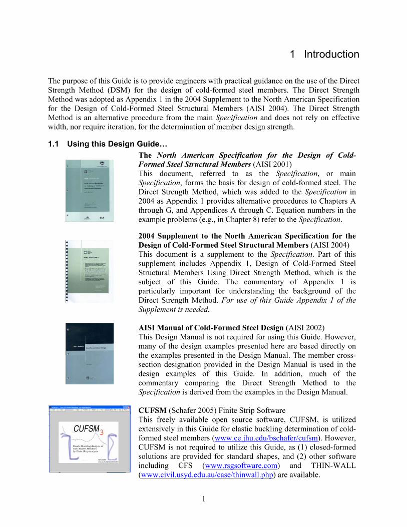
The North American Specification for the Design of Cold-Formed Steel Structural Members (AISI 2001) This document, referred to as the Specification, or main Specification, forms the basis for design of cold-formed steel. The Direct Strength Method, which was added to the Specification in 2004 as Appendix 1 provides alternative procedures to Chapters A through G, and Appendices A through C. Equation numbers in the example problems (e.g., in Chapter 8) refer to the Specification.
2004 Supplement to the North American Specification for the Design of Cold-Formed Steel Structural Members (AISI 2004) This document is a supplement to the Specification. Part of this supplement includes Appendix 1, Design of Cold-Formed Steel Structural Members Using Direct Strength Method, which is the subject of this Guide. The commentary of Appendix 1 is particularly important for understanding the background of the Direct Strength Method. For use of this Guide Appendix 1 of the Supplement is needed.
AISI Manual of Cold-Formed Steel Design (AISI 2002) This Design Manual is not required for using this Guide. However, many of the design examples presented here are based directly on the examples presented in the Design Manual. The member cross-section designation provided in the Design Manual is used in the design examples of this Guide. In addition, much of the commentary comparing the Direct Strength Method to the Specification is derived from the examples in the Design Manual.
CUFSM (Schafer 2005) Finite Strip Software This freely available open source software, CUFSM, is utilized extensively in this Guide for elastic buckling determination of cold-formed steel members (www.ce.jhu.edu/bschafer/cufsm). However, CUFSM is not required to utilize this Guide, as (1) closed-formed solutions are provided for standard shapes, and (2) other software including CFS (www.rsgsoftware.com) and THIN-WALL (www.civil.usyd.edu.au/case/thinwall.php) are available.

2
1.2 Why use DSM (Appendix 1) instead of the main Specification? The design of optimized cold-formed steel shapes is often completed more easily with the Direct Strength Method than with the main Specification. As Figure 1 indicates, DSM provides a design method for complex shapes that requires no more effort than for normal shapes, while the main Specification can be difficult, or even worse, simply inapplicable. Practical advantages of DSM:
• no effective width calculations, • no iterations required, and • uses gross cross-sectional properties.
Elastic buckling analysis performed on the computer (e.g., by CUFSM) is directly integrated into DSM. This provides a general method of designing cold-formed steel members and creates the potential for much broader extensions than the traditional Specification methods, that rely on closed-form solutions with limited applicability. Theoretical advantages of the DSM approach:
• explicit design method for distortional buckling, • includes interaction of elements (i.e., equilibrium
and compatibility between the flange and web is maintained in the elastic buckling prediction), and
• explores and includes all stability limit states. Philosophical advantages to the DSM approach:
• encourages cross-section optimization, • provides a solid basis for rational analysis extensions, • potential for much wider applicability and scope, and • engineering focus is on correct determination of elastic buckling behavior,
instead of on correct determination of empirical effective widths. Of course, numerous limitations of DSM (as implemented in AISI 2004) exist as well, not the least of which is that the method has only been formally developed for the determination of axial (Pn) and bending (Mn) strengths to date. A detailed list of limitations is presented and discussed in Section 1.4 of this Guide. Ongoing research and development is endeavoring to address and eliminate current limitations.
1.3 Designing with DSM (Appendix 1) and the main Specification The Direct Strength Method is part of the Specification, and was formally adopted as Appendix 1 (AISI 2004). The term “main Specification” refers to the Specification excluding Appendix 1. The Direct Strength Method provides alternative predictions for Mn and Pn that may be used in lieu of equations in the main Specification; see Section 1.3.1 and the examples of Chapter 8 in this Guide. When using Appendix 1 in conjunction with the main Specification reliability is maintained by the use of the φ and Ω factors given in Appendix 1 as discussed in Section 1.3.2 of this Guide. In some situations the Direct Strength Method may form the basis for a rational analysis extension to the Specification as discussed in A1.1(b) of the Specification and detailed further in Section 1.3.3 of this Guide.
(a) conventional shapes
design effort main Specification medium DSM (Appendix 1) medium
(b) optimized shapes
design effort main Specification high or NA* DSM (Appendix 1) medium *NA = not applicable or no design rules Figure 1 Cold-formed steel shapes

3
1.3.1 Approved usage, Mn and Pn DSM (Appendix 1 of AISI 2004) provides a strength prediction for Mn and Pn. These nominal flexural (beam) and axial (column) strengths are used in numerous sections of the main Specification. Table 1 below provides a roadmap for the replacement of Mn and Pn in the main Specification with the predicted values from Appendix 1. This table does not cover the extended use of DSM as a rational analysis tool, see Section 1.3.3 of this Guide.
Table 1 DSM alternative to main Specification calculations DSM calculation Provides an alternative to the main Specification
Mn
of 1.2.2 in App. 1
C3.1 Flexural Members – Bending • C3.1.1(a): DSM Mn is an alternative to Mn of C3.1.1(a) Nominal
Section Strength [Resistance] Procedure I • C3.1.2: DSM Mn is an alternative to Mn of C3.1.2 Lateral-
Torsional Buckling Strength [Resistance]
Mn with Mne=My* of 1.2.2 in App. 1
• C3.1.3: DSM Mn is an alternative to SeFy of C3.1.3 Beams Having One Flange Through-Fastened to Deck or Sheathing (R must still be determined from C3.1.3)
• C3.1.4: DSM Mn is an alternative to SeFy of C3.1.4 Beams Having One Flange Fastened to a Standing Seam Roof System (R must still be determined from C3.1.4)
Mn
of 1.2.2 in App. 1
C3.3, C3.5, C5.1, C5.2 Combined Bending (interaction equations) • C3.3: DSM Mn is an alternative to Mn of C3.3 Combined
Bending and Shear • C5.1: DSM Mn about x and y axes are alternatives to Mnx and Mny
of C5.1 Combined Tensile Axial Load and Bending • C5.2: DSM Mn about x and y axes are alternatives to Mnx and Mny
of C5.2 Combined Compressive Axial Load and Bending
Mn with Mne=My* of 1.2.2 in App. 1
• C3.3: DSM Mn is an alternative to Mnxo of C3.3 Combined Bending and Shear
• C3.5: DSM Mn is an alternative to Mnxo of C3.5 Combined Bending and Web Crippling, DSM 2Mn is an alternative to Mno of C3.5.1 and 2(c)
Pn
of 1.2.1 in App. 1
C4 Concentrically Loaded Compression Members • C4: DSM Pn is an alternative to Pn of C4 Concentrically Loaded
Compression Members. • C4.1 – C4.4: DSM Fcre is an alternative definition of Fe of
sections C4.1 – C4.4, CUFSM is used as a rational analysis for Fe as discussed in C4.4 Nonsymmetric Sections
Pn with Pne=Py
of 1.2.1 in App. 1
C3.6.2 Bearing Stiffeners (AISI 2004, Supplement) • C3.6.2: DSM Pn determined with Pne=Py is an alternative to AeFy
in C3.6.2 Bearing Stiffeners in C-Section Members. Pn
of 1.2.1 in App. 1 C5.2 Combined Bending (interaction equations)
• C5.2 DSM Pn is an alternative to Pn of C5.2 * In the main Specification to account for local buckling reductions of a fully braced beam the effective section modulus (Se) is determined at yield (Fy) in several sections. The resulting capacity SeFy may be replaced by an equivalent DSM (App. 1) prediction by setting Mne=My and then finding Mn via DSM (App. 1). Similarly for columns AeFy may be replaced by Pn determined with Pne=Py. See Chapter 8 for design examples.
4
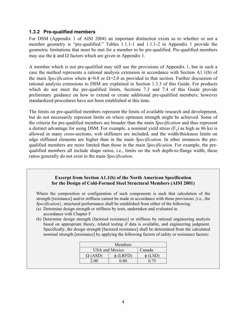
1.3.2 Pre-qualified members For DSM (Appendix 1 of AISI 2004) an important distinction exists as to whether or not a member geometry is “pre-qualified.” Tables 1.1.1-1 and 1.1.1-2 in Appendix 1 provide the geometric limitations that must be met for a member to be pre-qualified. Pre-qualified members may use the φ and Ω factors which are given in Appendix 1. A member which is not pre-qualified may still use the provisions of Appendix 1, but in such a case the method represents a rational analysis extension in accordance with Section A1.1(b) of the main Specification where φ=0.8 or Ω=2.0 as provided in that section. Further discussion of rational analysis extensions to DSM are explained in Section 1.3.3 of this Guide. For products which do not meet the pre-qualified limits, Sections 7.3 and 7.4 of this Guide provide preliminary guidance on how to extend or create additional pre-qualified members; however standardized procedures have not been established at this time. The limits on pre-qualified members represent the limits of available research and development, but do not necessarily represent limits on where optimum strength might be achieved. Some of the criteria for pre-qualified members are broader than the main Specification and thus represent a distinct advantage for using DSM. For example, a nominal yield stress (Fy) as high as 86 ksi is allowed in many cross-sections, web stiffeners are included, and the width/thickness limits on edge stiffened elements are higher than in the main Specification. In other instances the pre-qualified members are more limited than those in the main Specification. For example, the pre-qualified members all include shape ratios, i.e., limits on the web depth-to-flange width, these ratios generally do not exist in the main Specification.
Excerpt from Section A1.1(b) of the North American Specification
for the Design of Cold-Formed Steel Structural Members (AISI 2001) Where the composition or configuration of such components is such that calculation of the strength [resistance] and/or stiffness cannot be made in accordance with those provisions i.e., the Specification, structural performance shall be established from either of the following: (a) Determine design strength or stiffness by tests, undertaken and evaluated in
accordance with Chapter F (b) Determine design strength [factored resistance] or stiffness by rational engineering analysis
based on appropriate theory, related testing if data is available, and engineering judgment. Specifically, the design strength [factored resistance] shall be determined from the calculated nominal strength [resistance] by applying the following factors of safety or resistance factors:
Members
USA and Mexico Canada Ω (ASD) φ (LRFD) φ (LSD)
2.00 0.80 0.75
5
1.3.3 Rational analysis The development of DSM is incomplete. At this point only Mn and Pn are included. Further, many cross-sections that may be highly optimal for use in cold-formed steel structures fall outside of the scope of the main Specification and are not pre-qualified for DSM use. In such a situation an engineer is permitted to use rational analysis. Section A1.1(b) of the Specification specifically describes when rational analysis may be employed and an excerpt of this provision is provided on the previous page. The most obvious rational analysis extension of DSM is for cross-sections that are not pre-qualified, as discussed in Section 1.3.2 of this Guide. Such cross-sections may use the φ and Ω factors for rational analysis and then proceed to replace Mn and Pn in the main Specification as discussed in Section 1.3.1 of this Guide. A number of situations may exist where a rational analysis application of the DSM provisions is logical and worthy of pursuing. In general such an extension would include (1) determine the elastic buckling values for Mcrl, Mcrd, Mcre, Pcrl, Pcrd, Pcre for the unique situation envisioned, then (2) use the established DSM strength equations of Appendix 1 to determine Mn and Pn. Unique modeling may be required to determine the elastic buckling values. This may include specialized CUFSM analysis, specialized analytical methods, or general purpose finite element analysis (as discussed further in Chapter 2). Examples where a rational analysis extension to DSM of the nature described above might be considered include members: built-up from multiple cross-sections, with sheeting or sheathing on one side (flange) only, with dissimilar sheathing attached on two sides, with holes, or flanged holes, or with unique bracing (e.g., lip-to-lip braces which partially restrict distortional buckling). In addition, similar rational analysis extensions could allow an engineer to include the influence of moment gradient on all buckling modes, influence of different end conditions on all buckling modes, or influence of torsional warping stresses on all buckling modes. In other cases rational analysis extensions to DSM may be nothing more than dealing with the situation where an observed buckling mode is difficult to identify and making a judgment as to how to categorize the mode. The basic premise of DSM: extension of elastic buckling results to ultimate strength through the use of semi-empirical strength curves, is itself a rational analysis idea. DSM provides a basic roadmap for performing rational analysis in a number of unique situations encountered in cold-formed steel design.
6
1.4 Limitations of DSM: practical and theoretical Limitations of DSM (as implemented in AISI 2004)
• No shear provisions • No web crippling provisions • No provisions for members with holes • Limited number/geometry of pre-qualified members • No provisions for strength increase due to cold-work of forming
Discussion: Existing shear and web crippling provisions may be used when applicable. Otherwise, rational analysis or testing are a possible recourse. Members with holes are discussed further in Section 3.3.9 of this Guide, and this is a topic of current research. Pre-qualified members are discussed further in Section 1.3.2 and Chapter 7 of this Guide. Practical Limitations of DSM approach
• Overly conservative if very slender elements are used • Shift in the neutral axis is ignored • Empirical method calibrated only to work for cross-sections previously investigated
Discussion: DSM performs an elastic buckling analysis for the entire cross-section, not for the elements in isolation. If a small portion of the cross-section (a very slender element) initiates buckling for the cross-section, DSM will predict a low strength for the entire member. The effective width approach of the main Specification will only predict low strength for the offending element, but allow the rest of the elements making up the cross-section to carry load. As a result DSM can be overly conservative in such cases. The addition of stiffeners in the offending element may improve the strength, and the strength prediction, significantly. Shift in the neutral axis occurs when very slender elements are in compression in a cross-section. DSM conservatively accounts for such elements as described above, as such, ignoring the small shift has proven successful. The DSM strength equations are empirical, in much the same manner as the effective width equation, or the column curves; however, the range of cross-sections investigated is quite broad. Extension to completely unique cross-sections may require consideration of new or modified DSM strength expressions. Limitations of elastic buckling determination by finite strip method, as implemented in CUFSM
• Cross-section cannot vary along the length o no holes o no tapered members
• Loads cannot vary along the length (i.e., no moment gradient) • Global boundary conditions at the member ends are pinned (i.e., simply-supported) • Assignment of modes sometimes difficult, particularly for distortional buckling • Not readily automated due to manual need to identify the modes
Discussion: Chapter 2 and Section 3.3 of this Guide discuss elastic buckling determination, and the limitations of the finite strip method (e.g., CUFSM). Guidance on more robust alternatives using general purpose finite element analysis is given in Section 2.4 of this Guide.
7
2 Elastic buckling: Pcrl, Pcrd, Pcre, Mcrl, Mcrd, Mcre
The key to the flexibility of the Direct Strength Method is that no one particular method is prescribed for determining the elastic buckling loads and/or moments: Pcrl, Pcrd, Pcre, Mcrl, Mcrd, Mcre. Of course, this same flexibility may lead to some complications since a prescriptive path is not provided. This chapter of the Guide complements the commentary to the Direct Strength Method which provides significant discussion regarding elastic buckling determination. This chapter covers the definition of the basic buckling modes (Section 2.1) and provides guidance on when a mode can be ignored because it will not impact the strength prediction (Section 2.2). Four alternatives are provided and discussed for elastic buckling determination: finite strip (Section 2.3), finite element (Section 2.4), generalized beam theory (2.5), and closed-form solutions (Section 2.6).
WARNING Users are reminded that the strength of a member is not equivalent to the elastic buckling load (or moment) of the member. The elastic buckling load can be lower than the actual strength, for slender members with considerable post-buckling reserve; or the elastic buckling load can be fictitiously high due to ignoring inelastic effects. Nonetheless, the elastic buckling load is a useful reference for determining strength via the equations of the Direct Strength Method.

8
2.1 Local, Distortional, and Global Buckling The Direct Strength Method of Appendix 1 (AISI 2004) assigns the elastic buckling behavior into three classes: local (subscript ‘l’), distortional (subscript ‘d’), and global (subscript ‘e’, where the ‘e’ stands for Euler buckling). The DSM commentary (AISI 2004) defines elastic buckling and the three classes. The basic definitions are reviewed here for use in this Guide. Elastic buckling value is the load (or moment) at which the equilibrium of the member is neutral between two alternative states: the buckled shape and the original deformed shape. Local buckling involves significant distortion of the cross-section, but this distortion includes only rotation, not translation, at the internal fold lines (e.g., the corners) of a member. The half-wavelength of the local buckling mode should be less than or equal to the largest dimension of the member under compressive stress. Distortional buckling involves significant distortion of the cross-section, but this distortion includes rotation and translation at one or more internal fold lines of a member. The half-wavelength is load and geometry dependent, and falls between local and global buckling. Global buckling does not involve distortion of the cross-section, instead translation (flexure) and/or rotation (torsion) of the entire cross-section occurs. Global, or “Euler” buckling modes: flexural, torsional, torsional-flexural for columns, lateral-torsional for beams, occur as the minimum mode at long half-wavelengths. Research to provide more mechanics-based definitions that can be automatically implemented in finite strip and finite element software are underway (Schafer and Adany 2005), but at this time the phenomenon-based definitions given above represent the best available.
9
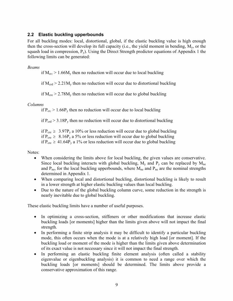
2.2 Elastic buckling upperbounds For all buckling modes: local, distortional, global, if the elastic buckling value is high enough then the cross-section will develop its full capacity (i.e., the yield moment in bending, My, or the squash load in compression, Py). Using the Direct Strength predictor equations of Appendix 1 the following limits can be generated: Beams
if Mcrl > 1.66My then no reduction will occur due to local buckling if Mcrd > 2.21My then no reduction will occur due to distortional buckling if Mcre > 2.78My then no reduction will occur due to global buckling
Columns
if Pcrl > 1.66Py then no reduction will occur due to local buckling if Pcrd > 3.18Py then no reduction will occur due to distortional buckling if Pcre ≥ 3.97Py a 10% or less reduction will occur due to global buckling if Pcre ≥ 8.16Py a 5% or less reduction will occur due to global buckling if Pcre ≥ 41.64Py a 1% or less reduction will occur due to global buckling
Notes:
• When considering the limits above for local buckling, the given values are conservative. Since local buckling interacts with global buckling, My and Py can be replaced by Mne and Pne, for the local buckling upperbounds, where Mne and Pne are the nominal strengths determined in Appendix 1.
• When comparing local and distortional buckling, distortional buckling is likely to result in a lower strength at higher elastic buckling values than local buckling.
• Due to the nature of the global buckling column curve, some reduction in the strength is nearly inevitable due to global buckling.
These elastic buckling limits have a number of useful purposes.
• In optimizing a cross-section, stiffeners or other modifications that increase elastic buckling loads [or moments] higher than the limits given above will not impact the final strength.
• In performing a finite strip analysis it may be difficult to identify a particular buckling mode, this often occurs when the mode is at a relatively high load [or moment]. If the buckling load or moment of the mode is higher than the limits given above determination of its exact value is not necessary since it will not impact the final strength.
• In performing an elastic buckling finite element analysis (often called a stability eigenvalue or eigenbuckling analysis) it is common to need a range over which the buckling loads [or moments] should be determined. The limits above provide a conservative approximation of this range.
10
2.3 Finite strip solutions This section of the Guide discusses basic elastic buckling determination using the finite strip method. The Direct Strength Method emphasizes the use of finite strip analysis for elastic buckling determination. Finite strip analysis is a general tool that provides accurate elastic buckling solutions with a minimum of effort and time. Finite strip analysis, as implemented in conventional programs, does have limitations, the two most important ones are
• the model assumes the ends of the member are simply-supported, and • the cross-section may not vary along its length.
These limitations preclude some analysis from readily being accomplished with the finite strip method, but despite these limitations the tool is useful, and a major advance over plate buckling solutions and plate buckling coefficients (k’s) that only partially account for the important stability behavior of cold-formed steel members. Overcoming specific difficulties associated with elastic buckling determination by the finite strip method is discussed in Section 3.3 of this Guide, following the detailed examples of Chapter 3 of this Guide.
2.3.1 CUFSM and other software The American Iron and Steel Institute has sponsored research that, in part, has led to the development of the freely available program, CUFSM, which employs the finite strip method for elastic buckling determination of any cold-formed steel cross-section. The program is available at www.ce.jhu.edu/bschafer/cufsm and runs on any PC with Windows 9x, NT, 2000, XP. Tutorials and examples are available online at the same address. The analyses performed in this Guide employ CUFSM. Users of this Guide are encouraged to download and use the software. The basic steps for performing any finite strip analysis are
• define the cross-section geometry, • determine the half-wavelengths to be investigated, • define the applied (reference) stress;
the results or load-factors are multipliers of this applied stress, • perform an elastic buckling analysis, and • examine the load-factor vs. half-wavelength curve to determine
minimum load-factors for each mode shape.
Finite strip software
At least three programs are known to provide elastic buckling by the finite strip method:
• CUFSM (www.ce.jhu.edu/bschafer/cufsm) • CFS (www.rsgsoftware.com), and • THIN-WALL (www.civil.usyd.edu.au/case/thinwall.php).

11
2.3.2 Interpreting a solution A finite strip analysis provides two results for understanding elastic buckling analysis, (1) the half-wavelength and corresponding load-factors, and (2) the cross-section mode (buckled) shapes. These two results are presented graphically in CUFSM as shown in Figure 2 along with discussions of the applied (reference) stress, which is what the load-factor (vertical axis of the response curve) refers to; minima, which are identified for each mode; half-wavelength, the longitudinal variation of the buckled shape; and mode shapes, the two-dimensional (2D) or cross-section variation of the buckled shape. For the example in Figure 2 of a 9CS2.5x059 (discussed further in Section 3.2.1 of this Guide), the applied (reference) stress is that of bending about the major axis, and the maximum stress is set equal to the yield stress of the material (55 ksi) so the applied reference stress is itself the yield moment, My. (Note, this definition of the yield moment is referenced to the nodal locations of the model which occur at the centerline of the thickness, not at the extreme fiber. For design practice the stress level at centerline of the thickness should be back-calculated with the yield stress occurring at the extreme fiber.) Facilities exist in CUFSM for generating and applying this stress, or other common stress distributions as applied (reference) stresses. The finite strip method always assumes the member buckles as a single half sine wave along the length. The length of this half sine wave is known as the half-wavelength. Finite strip analysis provides the buckling load [or moment] for all half-wavelengths selected by the user. Thus, finite strip analysis provides a means to understand all modes of buckling that might occur inside a given physical length (e.g., L=200 in. as shown in Figure 2). The actual member buckling mode (buckled shape) considered by FSM is:
Member buckling mode = 2D mode shape · sin(πx/half-wavelength)
In the example, the analysis has been performed at a large number of half-wavelengths. Resolution of the half-wavelength curve is only necessary to this level of accuracy near the minima. Two minima are identified from the curve:
• local buckling with an Mcrl = 0.67My and a half-wavelength of 5 in., and • distortional buckling with an Mcrd = 0.85My and a half-wavelength of 25 in..
Lateral-torsional buckling is identified at longer half-wavelengths. The exact value of Mcre
* that would be relevant would depend on the physical length of the member. The elastic buckling moment Mcre
* obtained from FSM does not take into account the influence of moment gradient, so Cb from the main Specification (Eq. C3.1.2.1-10) should be used to determine the elastic buckling value used in the Direct Strength Method, i.e., Mcre=CbMcre
*.

12
variation along the member length
half-wavelength
5 in. Local
25 in. Distortional
200 in. Lateral-torsional
5
Applied stress on the section indicates that a moment about the major axis is applied to this section. All results are given in reference to this applied stress distribution. Any axial stresses (due to bending, axial load, warping torsional stresses, or any combination thereof) may be considered in the analysis.
Minima indicate the lowest load level at which a particular mode of buckling occurs. The lowest Mcr/My is sought for each type of buck-ling. An identified cross-section mode shape can repeat along the physical length of the member.
Half-wavelength shows how a given cross-section mode shape (as shown in the figure) varies along its length.
Mode shapes are shown at the identified minima and at 200 in.. Identification of the mode shapes is critical to DSM, as each shape uses a different strength curve to connect the elastic buckling results shown here to the actual ultimate strength. In the section, local buckling only involves rotation at internal folds, distortionalbuckling involves both rotation and translation of internal fold lines, and lateral-torsional buckling involves “rigid-body”deformation of the cross-section without distortion.
UnderstandingFinite Strip Analysis Results
variation along the member length
half-wavelength
5 in. Local
25 in. Distortional
200 in. Lateral-torsional
5
Applied stress on the section indicates that a moment about the major axis is applied to this section. All results are given in reference to this applied stress distribution. Any axial stresses (due to bending, axial load, warping torsional stresses, or any combination thereof) may be considered in the analysis.
Minima indicate the lowest load level at which a particular mode of buckling occurs. The lowest Mcr/My is sought for each type of buck-ling. An identified cross-section mode shape can repeat along the physical length of the member.
Half-wavelength shows how a given cross-section mode shape (as shown in the figure) varies along its length.
Mode shapes are shown at the identified minima and at 200 in.. Identification of the mode shapes is critical to DSM, as each shape uses a different strength curve to connect the elastic buckling results shown here to the actual ultimate strength. In the section, local buckling only involves rotation at internal folds, distortionalbuckling involves both rotation and translation of internal fold lines, and lateral-torsional buckling involves “rigid-body”deformation of the cross-section without distortion.
UnderstandingFinite Strip Analysis Results
variation along the member length
half-wavelength
5 in. Local
25 in. Distortional
200 in. Lateral-torsional
5
Applied stress on the section indicates that a moment about the major axis is applied to this section. All results are given in reference to this applied stress distribution. Any axial stresses (due to bending, axial load, warping torsional stresses, or any combination thereof) may be considered in the analysis.
Minima indicate the lowest load level at which a particular mode of buckling occurs. The lowest Mcr/My is sought for each type of buck-ling. An identified cross-section mode shape can repeat along the physical length of the member.
Half-wavelength shows how a given cross-section mode shape (as shown in the figure) varies along its length.
Mode shapes are shown at the identified minima and at 200 in.. Identification of the mode shapes is critical to DSM, as each shape uses a different strength curve to connect the elastic buckling results shown here to the actual ultimate strength. In the section, local buckling only involves rotation at internal folds, distortionalbuckling involves both rotation and translation of internal fold lines, and lateral-torsional buckling involves “rigid-body”deformation of the cross-section without distortion.
Figure 2 Understanding Finite Strip Analysis Results

13
2.3.3 Ensuring an accurate solution In a typical finite strip analysis several variables are at the user’s discretion that influence the accuracy of the elastic buckling prediction, namely the number of elements in the cross-section, and the number of half-wavelengths used in the analysis. Elements: At least two elements should always be used in any portion of a plate that is subject to compression. This minimum number of elements ensures that a local buckling wave forming in the plate will be accurate to within 0.4% of the theoretical value. If a portion of the cross-section is subject to bending it is important to ensure at least two elements are in the compression region. When examining any buckling mode shape, at least two elements should form any local buckled wave, if there is only one, increase the number of elements. The impact of the number of elements selected is greatest on local buckling and less so on distortional and global buckling. Corners: It is recommended that when modeling smooth bends, such as at the corners of typical members, at least four elements are employed. This is a pragmatic recommendation based more on providing the correct initial geometry, rather than the impact of the corner itself on the solution accuracy. Unless the corner radius is large (e.g., r > 10t) use of centerline models that ignore the corner are adequate. The impact of corner radius is greatest on local buckling and less so on distortional and global buckling. Half-wavelengths: As shown in Figure 3, a sufficient number of lengths should be chosen to resolve the minima points from the finite strip analysis to within acceptable accuracy. Typically the local minimum will have a half-wavelength at or near the outer dimensions of the member; however, lengths as small as any flat portion of the cross-section should be included. Distortional buckling typically occurs between three to nine times the outer dimensions of the cross-section. Global buckling is usually best examined by selecting the physical member length of interest.
2.3.4 Programming classical finite strip analysis For readers who have programmed a conventional two dimensional matrix structural analysis code, developing a finite strip analysis code similar to CUFSM is readily doable. Cheung and Tham (1998) provide the most complete reference on the development of the finite strip method for use in solid mechanics. Schafer (1997), following Cheung’s approach, provides explicit derivations of the elastic and stability matrices employed in CUFSM. CUFSM itself is open source and the routines may be easily translated from Matlab into any modern programming language. The open source code for CUFSM and the relevant Chapter from Schafer (1997) are available online at www.ce.jhu.edu/bschafer/cufsm.
100
101
102
103
0
0.2
0.4
0.6
0.8
1
1.2
1.4
1.6
1.8
2
half-wavelength (in.)
Mcr
/My
curve with too few lengthsmore exact curve
distortional minimum missed
local minimum slightly off
100
101
102
103
0
0.2
0.4
0.6
0.8
1
1.2
1.4
1.6
1.8
2
half-wavelength (in.)
Mcr
/My
curve with too few lengthsmore exact curve
distortional minimum missed
local minimum slightly off
Figure 3 Importance of length selection
14
2.4 Finite element solutions This Guide cannot provide a full summary of the possible pitfalls with general purpose finite element (FE) analysis for elastic buckling (often termed eigenvalue buckling or eigen stability analysis) of cold-formed steel cross-sections. However, the use of general purpose FE analysis in the elastic buckling determination of cold-formed steel cross-sections is possible, and in some cases essentially the only known recourse. Plate or shell elements must be used to define the cross-section. References to basic FE texts on this subject are provided in the Direct Strength Method commentary (AISI 2004). A number of commercial FE implementations exist that the author of this guide has successfully used: ABAQUS, ANSYS, MSC/NASTRAN, STAGS. In addition, ADINA, and MARC are known to reliably provide solutions for elastic buckling of plates and shells. Other programs may work equally well. The rational analysis (see Section 1.3.3 of this Guide) extensions made possible by general purpose FE analysis include: the ability to handle any boundary condition, explicitly consider moment gradient, handle members with holes or thickness variation along the length, etc. These advantages make the use of FE analysis attractive. However, a number of theoretical and practical considerations must be handled, the most important of which are to perform benchmark problems on the elements and meshes being used, and to be patient and thorough in visually inspecting the buckling modes and identifying and assigning the buckled shapes to local, distortional, and global buckling. A discussion of some basic issues to consider when performing FE stability analysis follows. Benchmark problems with known classical solutions (e.g., see Timoshenko and Gere 1961, Allen and Bulson 1980, Galambos 1998) should be performed with any element and mesh being considered. Section 2.6 and Chapter 9 of this Guide provide a number of potential closed-form solutions which could be used for benchmark solutions. Numerical/theoretical FE issues
Element shape function: typically plate and shell elements use either linear (4 node shells) or polynomial shape functions (8 or 9 node shells) to determine how the element may deform. Regardless of the choice, a sufficient number of elements are required so that the element may adequately approximate the buckled shape of interest. A mesh convergence study with a simple benchmark problem is recommended.
Element aspect ratio: some plate and shell elements in current use will provide spurious solutions if the length/width of the element is too large or too small. Problematic element aspect ratios are element, geometry, and load dependent; however good practice is to keep elements at aspect ratios between 1:2 and 2:1, though between 1:4 and 4:1 is generally adequate.
Element choice: some plate and shell elements in current use have interpretations of the shear behavior more appropriate for moderately thick shells, as a result for thin plates common in cold-formed steel these elements may be overly soft or overly stiff in shear. This is most likely to impact distortional buckling predictions.

15
Practical FE issues
No half-wavelength curve: FE analysis is not performed at a variety of half-wavelengths. Varying the physical length in an FE analysis is not equivalent to varying the length in a finite strip analysis, since the longitudinal deformations possible in the FE analysis remain general (not restricted to single half sine waves). In FE analysis, all buckling modes that exist within a given physical length are examined, and the analyst must look through the modes to determine their classification: local, distortional, global. The maximum buckling value of interest is known (from the upperbounds of Section 2.2 of this Guide), but it is not known how many individual modes will be identified below this value.
Too many buckling modes are identified in a typical FE analysis for an expedient examination of the results; one must be patient and manually inspect the buckling modes. Expect to see similar buckling modes at many different half-wavelengths. It is not sufficient to identify only the minimum buckling mode. The minimum buckling value for each of the modes, local, distortional, and global needs to be identified. Engineering judgment will likely be required to identify all the modes, take care to ensure the deformed shapes are well represented by the selected element and mesh, consider performing supplementary analyses to verify results.
2.5 Generalized Beam Theory Elastic buckling determination may also be performed using the Generalized Beam Theory (GBT). GBT references are provided in the commentary to the Direct Strength Method. Although general purpose software is not currently available in the public domain, recently Camotim and Silvestre (2004) provided GBT code for a closed-form solution for distortional buckling of C’s and Z’s with ends that are pinned, free, or fixed. The code may be downloaded at www.ce.jhu.edu/bschafer/gbt and provides a means to handle the influence of boundary conditions on distortional buckling of traditional cold-formed steel shapes without recourse to general purpose FE solutions.
2.6 Manual elastic buckling solutions While the emphasis of the Direct Strength Method is on numerical solutions for elastic buckling, situations arise when manual (closed-form) solutions can be beneficial. Manual solutions may be used to provide a conservative check on more exact solutions, to readily automate elastic buckling solutions of a specific cross-section, or to help augment the identification of a particular mode in a more general numerical solution. The commentary to the Direct Strength Method provides extensive references for manual elastic buckling solutions of cold-formed steel members in local, distortional, and global buckling. In Chapter 9 of this Guide manual elastic buckling solutions of a cold-formed C are provided for local, distortional, and global buckling of both a column and a beam.
Can elastic buckling solutions be combined? Yes. It is possible that the most expedient solution for a given cross-section will be to perform finite strip or finite element analysis for local and distortional buckling, but use classical formulas for global buckling; or any combination thereof.
16
3 Member elastic buckling examples by the finite strip method
Examples of the elastic buckling determination for members by the finite strip method, and a detailed discussion of overcoming difficulties with elastic buckling, are the focus of this chapter of the Guide. Subsequently, the cross-sections analyzed in this chapter are used extensively to examine the design of beams (Chapter 4), columns (Chapter 5), and beam-columns (Chapter 6). Complete design examples for all the cross-sections covered in this chapter are provided in Chapter 8.
3.1 Construction of finite strip models Following the guidelines of Section 2.3.3 of this Guide a series of finite strip models were constructed. All of the models use centerline geometry for their calculation, and include corner radii. Inclusion of corner radii is not specifically necessary, but for a more exact comparison with existing models it was incorporated here.
3.2 Example cross-sections The examples presented include those of the AISI (2002) Design Manual plus additional examples selected to highlight the use of the Direct Strength Method for more complicated and optimized cross-sections. For each example the following is provided: (1) references to the AISI (2002) Design Manual example problems (as appropriate), (2) basic cross-section information and confirmation of finite strip model geometry, and (3) elastic buckling analysis by the finite strip method (CUFSM) and notes on analysis.
Models of the following cross-sections were generated: • C-section with lips, • C-section with lips modified, • C-section without lips (track section), • C-section without lips (track section) modified, • Z-section with lips, • Z-section with lips modified, • Equal leg angle with lips, • Equal leg angle, • Hat section, • Wall panel section, • Rack post section, and a • Sigma section.
Elastic buckling results are really just another property of the cross-section
The results presented here can be thought of as augmenting the “gross properties” of the cross-section. That is, Pcrl, Pcrd, Mcrl, Mcrd, augment A, I, etc. as properties of the cross-section, and can be calculated without knowledge of the application of the cross-section. In the future, the elastic buckling values studied in detail in this Chapter may simply be tabled for use by engineers.
17
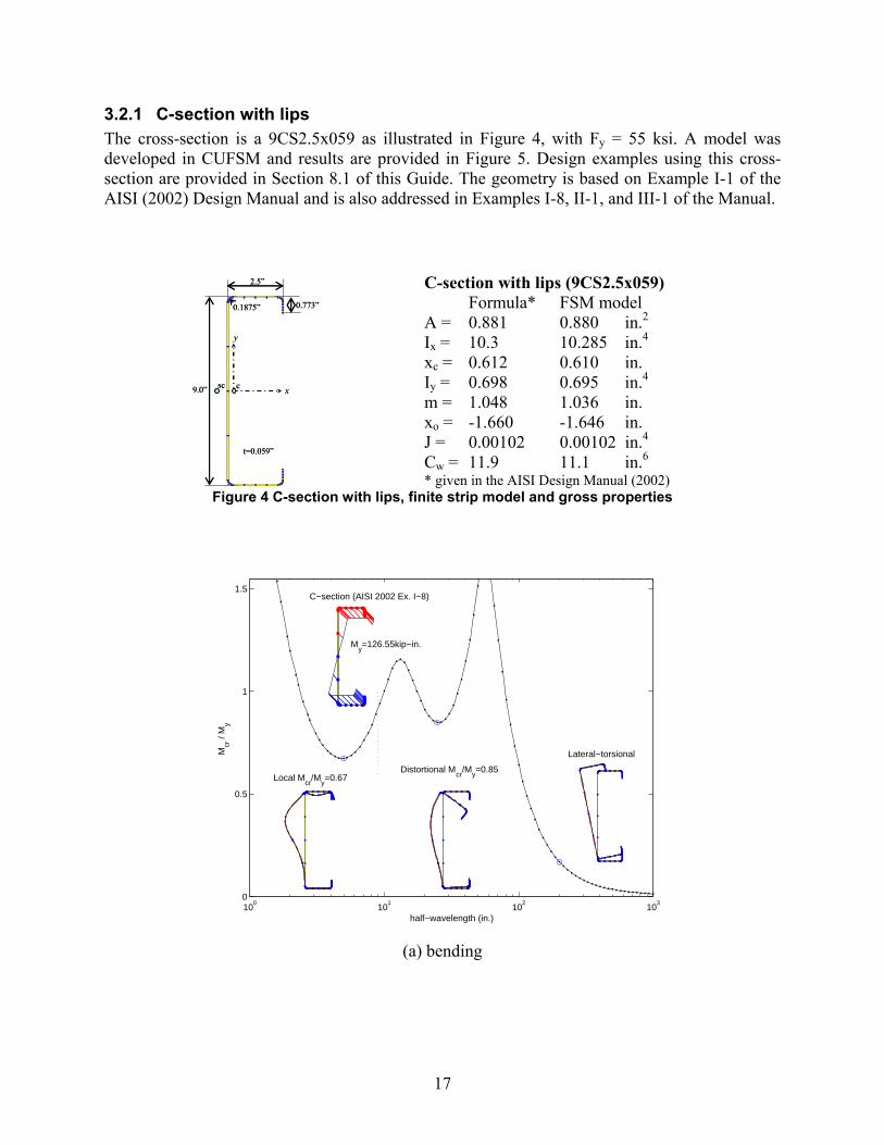
3.2.1 C-section with lips The cross-section is a 9CS2.5x059 as illustrated in Figure 4, with Fy = 55 ksi. A model was developed in CUFSM and results are provided in Figure 5. Design examples using this cross-section are provided in Section 8.1 of this Guide. The geometry is based on Example I-1 of the AISI (2002) Design Manual and is also addressed in Examples I-8, II-1, and III-1 of the Manual.
9.0”
2.5”
0.773”
t=0.059”
0.1875”
x
y
csc9.0”
2.5”
0.773”
t=0.059”
0.1875”
x
y
csc
C-section with lips (9CS2.5x059) Formula* FSM model A = 0.881 0.880 in.2 Ix = 10.3 10.285 in.4 xc = 0.612 0.610 in. Iy = 0.698 0.695 in.4 m = 1.048 1.036 in. xo = -1.660 -1.646 in. J = 0.00102 0.00102 in.4 Cw = 11.9 11.1 in.6 * given in the AISI Design Manual (2002)
Figure 4 C-section with lips, finite strip model and gross properties
100
101
102
103
0
0.5
1
1.5
half−wavelength (in.)
Mcr
/ M
y
C−section (AISI 2002 Ex. I−8)
My=126.55kip−in.
Local Mcr
/My=0.67
Distortional Mcr
/My=0.85
Lateral−torsional
(a) bending

18
100
101
102
103
0
0.05
0.1
0.15
0.2
0.25
0.3
0.35
0.4
half−wavelength (in.)
Pcr
/ P
y
C−section (AISI 2002 Ex. I−8)
Py=48.42kips
Local Pcr
/Py=0.12
Distortional Pcr
/Py=0.27
Flexural
(b) compression
Figure 5 C-section with lips, finite strip analysis results
Notes: • The circle “” at 200 in. in Figure 5a and b indicates the length from which the inset pictures
of the global buckling mode shape are generated from. This method of indicating the length for the related global buckling mode is similar throughout this Guide. Exact values for global buckling at a given length are provided in the Design Examples of Chapter 8 as needed.
• For the analysis in pure compression (Figure 5b) identification of the distortional mode is not readily apparent. In this case, examination of the buckling mode shape itself (as illustrated in the Figure) identifies the transition from local to distortional buckling.
• The local buckling mode shape for pure compression shows web local buckling, but little if any local buckling in the flange and lip. When one element dominates the behavior, the strength predictions via DSM may be conservative.
• My in this, and all, examples was generated using default options in CUFSM and thus includes the assumption that the maximum stress occurs at the centerline of the flange (location of the nodes in the model) instead of the extreme fiber. In this example the My reported above is 126.55 kip-in. and may be compared to (10.3 in.4/4.5 in.)(55 ksi) = 125.89 kip-in., a difference of 0.5%. For design practice, to have the maximum stress occur at the extreme fiber, the centerline stress should be back-calculated and entered into CUFSM.
See Section 8.1 of this Guide for a complete set of design examples using this cross-section.
!

19
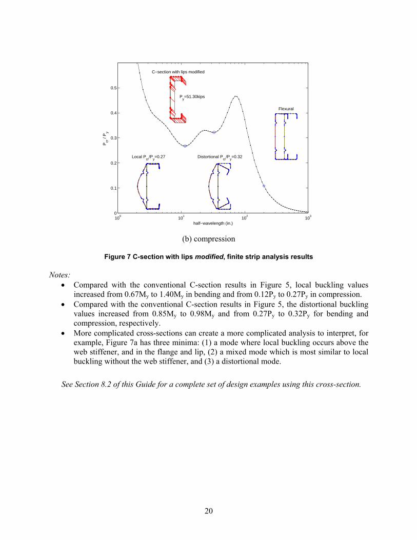
3.2.2 C-section with lips modified A modification of the C-section with lip (9CS2.5x059) from the previous cross-section was created to demonstrate how Appendix 1 may be applied to more unique cross-sections and to demonstrate potential preliminary steps towards cross-section optimization. The cross-section (Figure 6) has the same outer dimensions; however, 2 small ¼ in. stiffeners were added to the web, and the lip was lengthened from 0.773 in. to 1 in.. Global properties are changed only slightly, so the improvement is related to local and distortional, not global, buckling. Fy remains at 55 ksi.
9.0”
2.5”
1.0”
0.25”
1.8”0.1875”
t = 0.059”
x
y
cs
0.50”
C-section with lips modified Before After A = 0.880 0.933 in.2 Ix = 10.285 10.818 in.4 xc = 0.610 0.659 in. Iy = 0.695 0.781 in.4 m = 1.036 1.078 in. xo = -1.646 -1.859 in. J = 0.00102 0.00108 in.4 Cw = 11.1 13.33 in.6
Figure 6 C-section with lips modified, finite strip model and gross properties
100
101
102
103
0
0.2
0.4
0.6
0.8
1
1.2
1.4
1.6
1.8
2
half−wavelength (in.)
Mcr
/ M
y
C−section with lips modified
My=133.08kip−in.
Mcr
/My=1.50
Mcr
/My=0.98
Lateral−torsional
Mcr
/My=1.40
Distortional
(a) bending
20
100
101
102
103
0
0.1
0.2
0.3
0.4
0.5
half−wavelength (in.)
Pcr
/ P
y
C−section with lips modified
Py=51.30kips
Local Pcr
/Py=0.27 Distortional P
cr/P
y=0.32
Flexural
(b) compression
Figure 7 C-section with lips modified, finite strip analysis results
Notes:
• Compared with the conventional C-section results in Figure 5, local buckling values increased from 0.67My to 1.40My in bending and from 0.12Py to 0.27Py in compression.
• Compared with the conventional C-section results in Figure 5, the distortional buckling values increased from 0.85My to 0.98My and from 0.27Py to 0.32Py for bending and compression, respectively.
• More complicated cross-sections can create a more complicated analysis to interpret, for example, Figure 7a has three minima: (1) a mode where local buckling occurs above the web stiffener, and in the flange and lip, (2) a mixed mode which is most similar to local buckling without the web stiffener, and (3) a distortional mode.
See Section 8.2 of this Guide for a complete set of design examples using this cross-section.
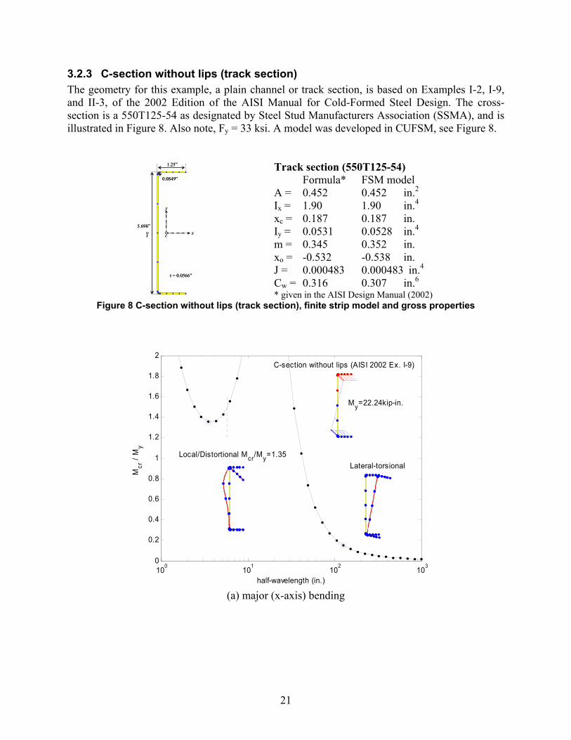
21
3.2.3 C-section without lips (track section) The geometry for this example, a plain channel or track section, is based on Examples I-2, I-9, and II-3, of the 2002 Edition of the AISI Manual for Cold-Formed Steel Design. The cross-section is a 550T125-54 as designated by Steel Stud Manufacturers Association (SSMA), and is illustrated in Figure 8. Also note, Fy = 33 ksi. A model was developed in CUFSM, see Figure 8.
5.698”
1.25”
0.0849”
t = 0.0566”
x
y
cs
5.698”
1.25”
0.0849”
t = 0.0566”
x
y
cs
Track section (550T125-54) Formula* FSM model A = 0.452 0.452 in.2 Ix = 1.90 1.90 in.4 xc = 0.187 0.187 in. Iy = 0.0531 0.0528 in.4 m = 0.345 0.352 in. xo = -0.532 -0.538 in. J = 0.000483 0.000483 in.4 Cw = 0.316 0.307 in.6 * given in the AISI Design Manual (2002)
Figure 8 C-section without lips (track section), finite strip model and gross properties
100 101 102 1030
0.2
0.4
0.6
0.8
1
1.2
1.4
1.6
1.8
2
half-wavelength (in.)
Mcr
/ M
y
C-section without lips (AISI 2002 Ex. I-9)
My=22.24kip-in.
Local/Distortional Mcr/My=1.35Lateral-torsional
(a) major (x-axis) bending
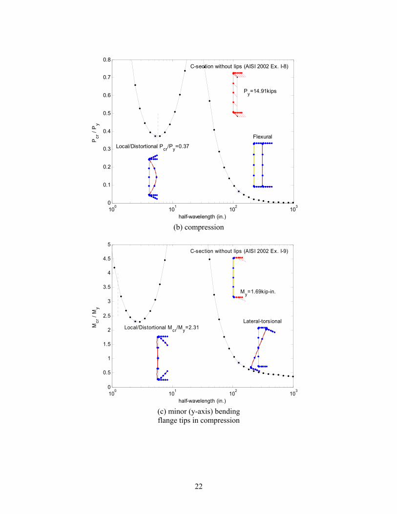
22
100 101 102 1030
0.1
0.2
0.3
0.4
0.5
0.6
0.7
0.8
half-wavelength (in.)
Pcr
/ P
y
C-section without lips (AISI 2002 Ex. I-8)
Py=14.91kips
Local/Distortional Pcr/Py=0.37
Flexural
(b) compression
100
101
102
103
0
0.5
1
1.5
2
2.5
3
3.5
4
4.5
5
half-wavelength (in.)
Mcr
/ M
y
C-section without lips (AISI 2002 Ex. I-9)
My=1.69kip-in.
Local/Distortional Mcr/My=2.31Lateral-torsional
(c) minor (y-axis) bending flange tips in compression

23
100
101
102
103
0
0.5
1
1.5
2
2.5
3
3.5
4
4.5
5
half-wavelength (in.)
Mcr
/ M
y
C-section without lips (AISI 2002 Ex. I-9)
My=1.69kip-in.
Local Mcr/My=2.52
(d) minor (y-axis) bending
flange tips in tension
Figure 9 C-section without lips (track section), finite strip analysis results
See Section 8.3 of this Guide for a complete set of design examples using this cross-section.
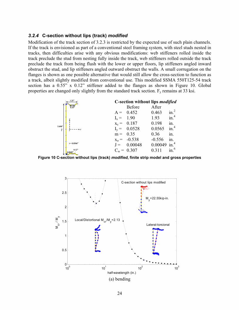
24
3.2.4 C-section without lips (track) modified Modification of the track section of 3.2.3 is restricted by the expected use of such plain channels. If the track is envisioned as part of a conventional steel framing system, with steel studs nested in tracks, then difficulties arise with any obvious modifications: web stiffeners rolled inside the track preclude the stud from nesting fully inside the track, web stiffeners rolled outside the track preclude the track from being flush with the lower or upper floors, lip stiffeners angled inward obstruct the stud, and lip stiffeners angled outward obstruct the walls. A small corrugation on the flanges is shown as one possible alternative that would still allow the cross-section to function as a track, albeit slightly modified from conventional use. This modified SSMA 550T125-54 track section has a 0.55” x 0.12” stiffener added to the flanges as shown in Figure 10. Global properties are changed only slightly from the standard track section. Fy remains at 33 ksi.
5.698”
1.25”
0.0849”
t = 0.0566”
x
y
cs
0.12”
0.55”
5.698”
1.25”
0.0849”
t = 0.0566”
x
y
cs
0.12”
0.55”
C-section without lips modified Before After A = 0.452 0.463 in.2 Ix = 1.90 1.93 in.4 xc = 0.187 0.198 in. Iy = 0.0528 0.0565 in.4 m = 0.35 0.36 in. xo = -0.538 -0.556 in. J = 0.00048 0.00049 in.4 Cw = 0.307 0.311 in.6
Figure 10 C-section without lips (track) modified, finite strip model and gross properties
100
101
102
103
0
0.5
1
1.5
2
2.5
3
half-wavelength (in.)
Mcr
/ M
y
C-section without lips modified
My=22.55kip-in.
Local/Distortional Mcr/My=2.13Lateral-torsional
(a) bending
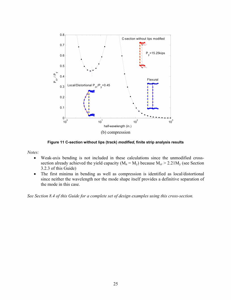
25
100
101
102
103
0
0.1
0.2
0.3
0.4
0.5
0.6
0.7
0.8
half-wavelength (in.)
Pcr
/ P
y
C-section without lips modified
Py=15.25kips
Local/Distortional Pcr/Py=0.45
Flexural
(b) compression
Figure 11 C-section without lips (track) modified, finite strip analysis results
Notes:
• Weak-axis bending is not included in these calculations since the unmodified cross-section already achieved the yield capacity (Mn = My) because Mcr > 2.21My (see Section 3.2.3 of this Guide)
• The first minima in bending as well as compression is identified as local/distortional since neither the wavelength nor the mode shape itself provides a definitive separation of the mode in this case.
See Section 8.4 of this Guide for a complete set of design examples using this cross-section.

26
3.2.5 Z-section with lips The geometry for this example, a Z-section, is based on Examples I-3, I-10, II-2, and III-6 of the 2002 Edition of the AISI Manual for Cold-Formed Steel Design. The cross-section is a 8ZS2.25x059, and is illustrated in Figure 12. Also note, Fy = 55 ksi. A model was developed in CUFSM for finite strip analysis, Figure 12 illustrates the node locations of the model, a comparison of calculated cross-section properties is also provided.
C x
y
1
1
2
2
8.0”
2.25”
t = 0.059”
0.91”
C x
y
1
1
2
2
8.0”
2.25”
t = 0.059”
0.91”
Z-section 8ZS2.25x059 Formula* FSM model A = 0.822 0.822 in.2 Ix = 7.763 7.762 in.4 Iy = 1.076 1.079 in.4 Ixy = 2.082 2.086 in.4 θ = 74 74 º I2 = 0.481 0.481 in.4 I1 = 8.36 8.36 in.4 J = 0.000954 0.000954 in.4 Cw = 12.6 12.5 in.6 * given in the AISI Design Manual (2002)
Figure 12 Z-section with lips, finite strip model and gross properties
100
101
102
103
0
0.5
1
1.5
half-wavelength (in.)
Mcr
/ M
y
Z-section (AISI 2002 Ex. I-10)
My=107.53kip-in.
Local Mcr/My=0.85Distortional Mcr/My=0.77
Lateral-torsional
(a) restrained bending about x-axis
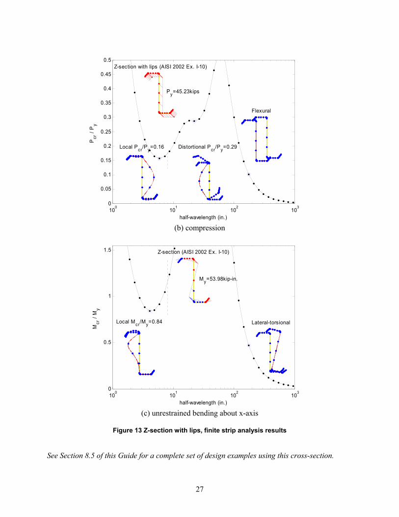
27
100
101
102
103
0
0.05
0.1
0.15
0.2
0.25
0.3
0.35
0.4
0.45
0.5
half-wavelength (in.)
Pcr
/ P
y
Z-section with lips (AISI 2002 Ex. I-10)
Py=45.23kips
Local Pcr/Py=0.16 Distortional Pcr/Py=0.29
Flexural
(b) compression
100
101
102
103
0
0.5
1
1.5
half-wavelength (in.)
Mcr
/ M
y
Z-section (AISI 2002 Ex. I-10)
My=53.98kip-in.
Local Mcr/My=0.84 Lateral-torsional
(c) unrestrained bending about x-axis
Figure 13 Z-section with lips, finite strip analysis results
See Section 8.5 of this Guide for a complete set of design examples using this cross-section.
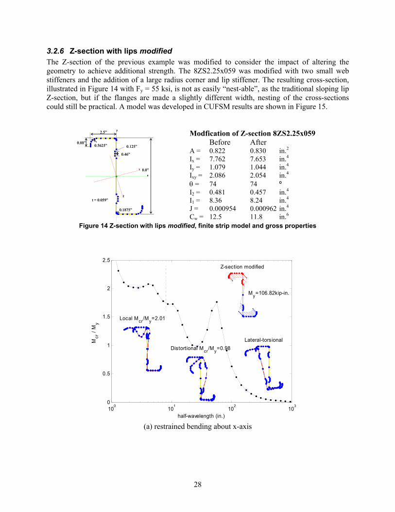
28
3.2.6 Z-section with lips modified The Z-section of the previous example was modified to consider the impact of altering the geometry to achieve additional strength. The 8ZS2.25x059 was modified with two small web stiffeners and the addition of a large radius corner and lip stiffener. The resulting cross-section, illustrated in Figure 14 with Fy = 55 ksi, is not as easily “nest-able”, as the traditional sloping lip Z-section, but if the flanges are made a slightly different width, nesting of the cross-sections could still be practical. A model was developed in CUFSM results are shown in Figure 15.
x
y
1
2
8.0”
2.5”
t = 0.059”
0.88”0.5625”
0.1875”
0.46”
0.125”
x
y
1
2
8.0”
2.5”
t = 0.059”
0.88”0.5625”
0.1875”
0.46”
0.125”
Modfication of Z-section 8ZS2.25x059 Before After A = 0.822 0.830 in.2 Ix = 7.762 7.653 in.4 Iy = 1.079 1.044 in.4 Ixy = 2.086 2.054 in.4 θ = 74 74 º I2 = 0.481 0.457 in.4 I1 = 8.36 8.24 in.4 J = 0.000954 0.000962 in.4 Cw = 12.5 11.8 in.6
Figure 14 Z-section with lips modified, finite strip model and gross properties
100
101
102
103
0
0.5
1
1.5
2
2.5
half-wavelength (in.)
Mcr
/ M
y
Z-section modified
My=106.82kip-in.
Local Mcr/My=2.01
Distortional Mcr/My=0.98Lateral-torsional
(a) restrained bending about x-axis

29
100
101
102
103
0
0.1
0.2
0.3
0.4
0.5
half-wavelength (in.)
Pcr
/ P
y
Z-section modified
Py=45.64kips
Local Pcr/Py=0.27 Distortional Pcr/Py=0.33
Flexural
(b) compression
Figure 15 Z-section with lips modified, finite strip analysis results
Notes:
• The improvement in local buckling (from the unmodified Z) is essentially all attributable to the addition of the web stiffeners.
• The improvement in distortional buckling (from the unmodified Z) is essentially all attributable to the changes in the lip stiffener geometry.
• Separate models with only the web stiffeners added to the original Z-section, or only the lip stiffener modified, were evaluated and support the above two notes.
See Section 8.6 of this Guide for a complete set of design examples using this cross-section.

30
3.2.7 Equal leg angle with lips The geometry geometry for an equal leg angle with lips is based on Examples I-4, I-11, and III-4 of the 2002 Edition of the AISI Manual for Cold-Formed Steel Design. The cross-section is a 4LS4x060 as illustrated in Figure 16, with Fy = 50 ksi. Results from the CUFSM finite strip analysis are given in Figure 17.
C x
y
1
1
2
2
4.0”
4.0”
0.5”
0.5”
0.1875”
C x
y
1
1
2
2
C x
y
1
1
2
2
4.0”
4.0”
0.5”
0.5”
0.1875”
Equal leg angle with lips (4LS4x060) Formula* FSM model A = 0.512 0.512 in.2 Ix,Iy = 0.958 0.958 in.4 xc = 1.097 1.096 in. Ixy = -0.562 -0.561 in.4 I2 = 0.396 0.397 in.4 m = 0.083 0.083 in. xo = -1.634 -1.633 in. J = 0.000615 0.000615 in.4 * given in the AISI Design Manual (2002)
Figure 16 Equal leg angle with lips, finite strip model and gross properties
100 101 102 1030
0.2
0.4
0.6
0.8
1
1.2
1.4
1.6
1.8
2
half-wavelength (in.)
Mcr
/ M
y
Angle with lips (AISI 2002 Ex. I-11)
My=16.85kip-in.Local Mcr/My=1.69
Distortional
Lateral-torsional
(a) bending (geometric/restrained bending)

31
100 101 102 1030
0.1
0.2
0.3
0.4
0.5
0.6
half-wavelength (in.)
Pcr
/ P
y
Angle with lips (AISI 2002 Ex. I-11)
Py=25.61kips
Local Pcr/Py=0.53
Torsional (Distortional)
Flexural (primary axis)
(b) compression
100 101 1020
1
2
3
4
5
6
half-wavelength (in.)
Mcr
/ M
y
Angle with lips (AISI 2002 Ex. I-11)
My=12.66kip-in.Local Mcr/My=4.93
Torsional Mcr/My=0.69
(c) bending about the min. principal axis(flange tips in compression)
Figure 17 Equal leg angle with lips, finite strip analysis results Notes:
• In bending, distortional buckling of the stiffened leg is not discretely identifiable from long-wavelength LTB (no minimum in the FSM curve). In a design the distortional buckling value (Mcr/My) at the design unbraced length should be used to determine if distortional buckling is relevant to the behavior.
• In compression, “distortional buckling” of the stiffened legs is essentially torsional buckling of the angle. The second (higher) buckling mode is presented as a dashed line in Figure 17b. It can be seen that at long half-wavelengths flexural buckling about the minor principal axis (2-2) occurs at lower levels than torsional buckling.
See Section 8.7 of this Guide for a complete set of design examples using this cross-section.

32
3.2.8 Equal leg angle The geometry selected for an equal leg angle is based on Examples I-5, and I-12 of the 2002 Edition of the AISI Manual for Cold-Formed Steel Design. The cross-section is a 2LU2x060 as illustrated in Figure 18, with Fy = 33 ksi. A model was developed in CUFSM for finite strip analysis, results are shown in Figure 19.
C x
y
1
2
2.0”
2.0”
0.1875” t=0.06”
C x
y
1
2
2.0”
2.0”
0.1875” t=0.06”
Equal leg angle (2LU2x060) Formula* FSM model A = 0.231 0.231 in.2 Ix,Iy = 0.094 0.094 in.4 xc = 0.505 0.506 in. Ixy = -0.0589 -0.0589 in.4 I2 = 0.0351 0.0350 in.4 m = 0.0 0.0117 in. xo = -0.714 -0.702 in. J = 0.000277 0.000277 in.4 * given in the AISI Design Manual (2002)
Figure 18 Equal leg angle, finite strip model and gross properties
100 101 102 1030
0.2
0.4
0.6
0.8
1
1.2
1.4
1.6
1.8
2
half-wavelength (in.)
Mcr
/ M
y
Angle (AISI 2002 Ex. I-12)
My=2.12kip-in.
Local/Distortional Mcr/My=1.03
Lateral-torsional
(a) bending (restrained bending)

33
100
101
102
103
0
0.1
0.2
0.3
0.4
0.5
0.6
0.7
0.8
0.9
half-wavelength (in.)
Pcr
/ P
y
Angle (AISI 2002 Ex. I-12)
Py=7.61kips
Local/Distortional/Torsional
Flexural (primary axis)
(b) compression
Figure 19 Equal leg angle, finite strip analysis results
Notes:
• In bending (restrained bending about the x-axis) it is conservatively assumed that the first minimum is either local or distortional buckling. Based on the half-wavelength, as discussed in the DSM commentary (AISI 2004), this mode could be identified as distortional, but without an edge stiffener it has generally been considered a local mode.
• In compression, no minima exist – the analysis is always dependent on the unbraced length. At short to intermediate lengths a torsional mode dominates the buckling deformation, while at long lengths the flexural mode about the minor principal (2-2) axis dominates. For bracing to be adequate it must restrict the appropriate deformation, twist for lengths less than ~ 60 in., and bending about the minor axis for longer lengths.
See Section 8.8 of this Guide for a complete set of design examples using this cross-section.
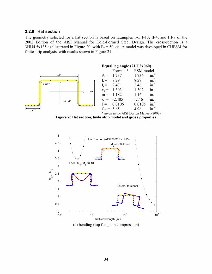
34
3.2.9 Hat section The geometry selected for a hat section is based on Examples I-6, I-13, II-4, and III-8 of the 2002 Edition of the AISI Manual for Cold-Formed Steel Design. The cross-section is a 3HU4.5x135 as illustrated in Figure 20, with Fy = 50 ksi. A model was developed in CUFSM for finite strip analysis, with results shown in Figure 21.
3.0”
4.5”
1.67”
0.1875”
t=0.135”
x
y 3.0”
4.5”
1.67”
0.1875”
t=0.135”
x
y
Equal leg angle (2LU2x060) Formula* FSM model A = 1.737 1.736 in.2 Ix = 8.29 8.29 in.4 Iy = 2.47 2.46 in.4
xc = 1.303 1.302 in. m = 1.182 1.16 in. xo = -2.485 -2.46 in. J = 0.0106 0.0105 in.4 Cw = 5.65 4.96 in.6 * given in the AISI Design Manual (2002)
Figure 20 Hat section, finite strip model and gross properties
100 101 102 1030
0.5
1
1.5
2
2.5
3
3.5
4
4.5
5
half-wavelength (in.)
Mcr
/ M
y
Hat Section (AISI 2002 Ex. I-13)
My=79.09kip-in.
Local Mcr/My=3.48
Lateral-torsional
(a) bending (top flange in compression)

35
100
101
102
103
0
0.5
1
1.5
2
2.5
3
3.5
half-wavelength (in.)
Pcr
/ P
y
Hat section (AISI 2002 Ex. I-13)
Py=86.82kipsLocal Pcr/Py=2.65
Flexural-torsional Flexural
(b) compression
Figure 21 Hat section, finite strip analysis results
Notes:
• This hat section is relatively thick and local buckling occurs at high values (compare with the upperbounds established in Section 2.2 of this Guide), the only anticipated reductions in such a cross-section would be due to long unbraced lengths.
• Distortional buckling is not relevant to the performance of this cross-section in bending with the top flange in compression (Figure 21a).
• Distortional buckling occurs at too high of a stress to be relevant to the behavior of the column (Figure 21b).
• For long columns, the minimum mode switches from torsional-flexural to weak-axis flexural as the column length increases, at approximately 300 in. (25 ft).
See Section 8.9 of this Guide for a complete set of design examples using this cross-section.

36
3.2.10 Wall panel section The geometry selected for a wall panel is based on Examples I-7, I-14, of the 2002 Edition of the AISI Manual for Cold-Formed Steel Design. The cross-section is a 14 in. x 2 in. panel as illustrated in Figure 22, with Fy = 50 ksi. A model was developed in CUFSM for finite strip analysis (Figure 22), with results shown in Figure 23.
3” 3” 3” 3” 2”14”
2”
.25” .415”
r =.125”.35”t = 0.030”
3” 3” 3” 3” 2”14”
2”
.25” .415”
r =.125”.35”t = 0.030”
Wall Panel Section Formula* FSM model A = 0.585 0.585 in.2 Ix = 0.444 0.444 in.4 yc = 1.186 1.186 in. (referenced from top fiber) * given in the AISI Design Manual (2002)
Figure 22 Wall Panel section, finite strip model and gross properties
100
101
102
0
0.1
0.2
0.3
0.4
0.5
0.6
0.7
0.8
0.9
1
half-wavelength (in.)
Mcr
/ M
y
Panel (AISI 2002 Ex. I-14)
My=18.98kip-in.
Local Mcr/My=0.36
Distortional Mcr/My=0.55
(a) bending (top flange in compression)
panel edges left free
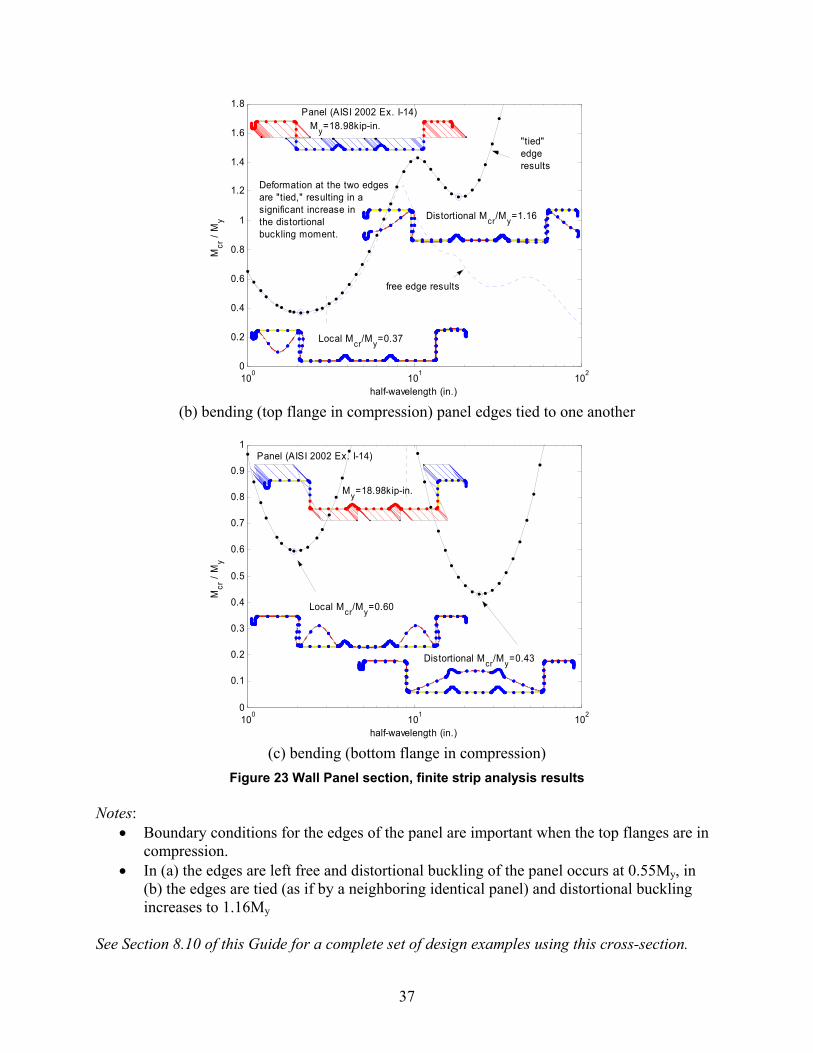
37
100 101 1020
0.2
0.4
0.6
0.8
1
1.2
1.4
1.6
1.8
half-wavelength (in.)
Mcr
/ M
y
Panel (AISI 2002 Ex. I-14)My=18.98kip-in.
Local Mcr/My=0.37
Distortional Mcr/My=1.16
Deformation at the two edgesare "tied," resulting in a significant increase inthe distortional buckling moment.
free edge results
"tied"edgeresults
(b) bending (top flange in compression) panel edges tied to one another
100 101 1020
0.1
0.2
0.3
0.4
0.5
0.6
0.7
0.8
0.9
1
half-wavelength (in.)
Mcr
/ M
y
Panel (AISI 2002 Ex. I-14)
My=18.98kip-in.
Local Mcr/My=0.60
Distortional Mcr/My=0.43
(c) bending (bottom flange in compression)
Figure 23 Wall Panel section, finite strip analysis results Notes:
• Boundary conditions for the edges of the panel are important when the top flanges are in compression.
• In (a) the edges are left free and distortional buckling of the panel occurs at 0.55My, in (b) the edges are tied (as if by a neighboring identical panel) and distortional buckling increases to 1.16My
See Section 8.10 of this Guide for a complete set of design examples using this cross-section.
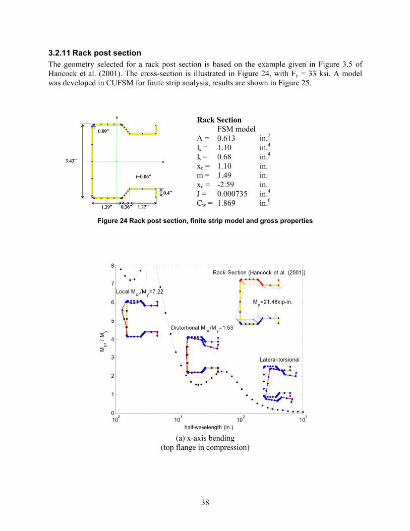
38
3.2.11 Rack post section The geometry selected for a rack post section is based on the example given in Figure 3.5 of Hancock et al. (2001). The cross-section is illustrated in Figure 24, with Fy = 33 ksi. A model was developed in CUFSM for finite strip analysis, results are shown in Figure 25.
x
y
3.43”
1.39”
0.09”
t=0.06”
1.22”
0.4”
0.36”
x
y
3.43”
1.39”
0.09”
t=0.06”
1.22”
0.4”
0.36”
Rack Section FSM model A = 0.613 in.2 Ix = 1.10 in.4 Iy = 0.68 in.4
xc = 1.10 in. m = 1.49 in. xo = -2.59 in. J = 0.000735 in.4 Cw = 1.869 in.6
Figure 24 Rack post section, finite strip model and gross properties
100
101
102
103
0
1
2
3
4
5
6
7
8
half-wavelength (in.)
Mcr
/ M
y
Rack Section (Hancock et al. (2001))
My=21.48kip-in.
Local Mcr/My=7.22
Distortional Mcr/My=1.53
Lateral-torsional
(a) x-axis bending
(top flange in compression)
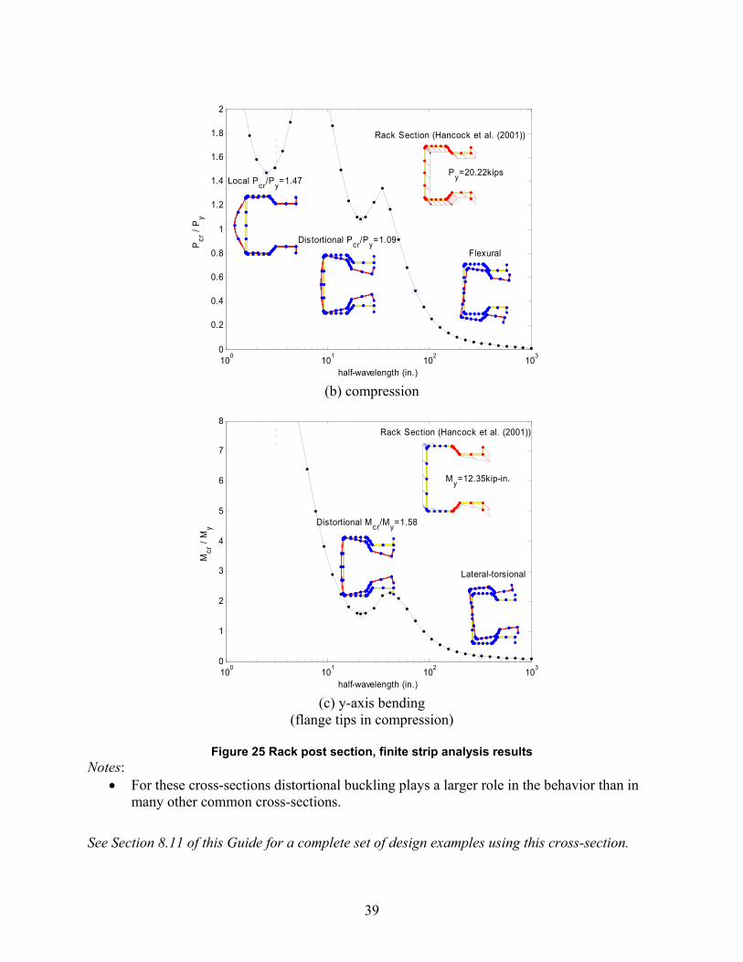
39
100 101 102 1030
0.2
0.4
0.6
0.8
1
1.2
1.4
1.6
1.8
2
half-wavelength (in.)
Pcr
/ P
y
Rack Section (Hancock et al. (2001))
Py=20.22kipsLocal Pcr/Py=1.47
Distortional Pcr/Py=1.09Flexural
(b) compression
100 101 102 1030
1
2
3
4
5
6
7
8
half-wavelength (in.)
Mcr
/ M
y
Rack Section (Hancock et al. (2001))
My=12.35kip-in.
Distortional Mcr/My=1.58
Lateral-torsional
(c) y-axis bending
(flange tips in compression)
Figure 25 Rack post section, finite strip analysis results Notes:
• For these cross-sections distortional buckling plays a larger role in the behavior than in many other common cross-sections.
See Section 8.11 of this Guide for a complete set of design examples using this cross-section.

40
3.2.12 Sigma section The geometry selected for a sigma section approximates a commercially available cross-section and is provided in Figure 26, where Fy = 50 ksi. No standard designation system exists for this cross-section type, but this member is designated as 800SG250-43. A model was developed in CUFSM, results are shown in Figure 27.
C x
y
8”
2.5”
2.25
”
1”
2.25
”
.875”
.5”
.625
”
t = 0.0451”r = 0.105”
(centerline model)
C x
y
8”
2.5”
2.25
”
1”
2.25
”
.875”
.5”
.625
”
t = 0.0451”r = 0.105”
(centerline model)
Sigma Section FSM model A = 0.747 in.2 Ix = 6.878 in.4 Iy = 0.576 in.4
xc = 0.940 in. m = 0.425 in. xo = -1.365 in. J = 0.000507 in.4 Cw = 11.07 in.6
Figure 26 Sigma section, finite strip model and gross properties
100
101
102
103
0
0.2
0.4
0.6
0.8
1
1.2
1.4
1.6
1.8
2
half-wavelength (in.)
Mcr
/ M
y
Sigma (800SG250-43)
My=86.40kip-in.
Local Mcr/My=0.96 Distortional Mcr/My=1.16
Lateral-torsional
(a) major axis bending
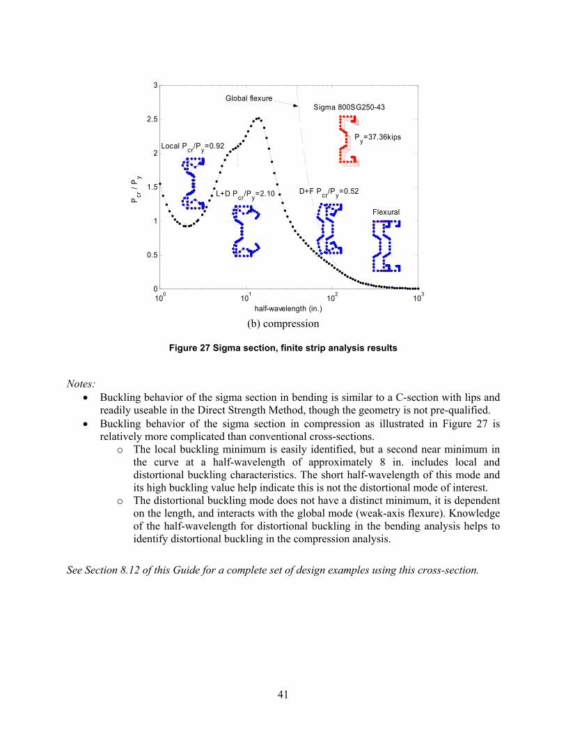
41
100
101
102
103
0
0.5
1
1.5
2
2.5
3
half-wavelength (in.)
Pcr
/ P
y
Sigma 800SG250-43
Py=37.36kipsLocal Pcr/Py=0.92
L+D Pcr/Py=2.10 D+F Pcr/Py=0.52
Flexural
Global flexure
(b) compression
Figure 27 Sigma section, finite strip analysis results
Notes: • Buckling behavior of the sigma section in bending is similar to a C-section with lips and
readily useable in the Direct Strength Method, though the geometry is not pre-qualified. • Buckling behavior of the sigma section in compression as illustrated in Figure 27 is
relatively more complicated than conventional cross-sections. o The local buckling minimum is easily identified, but a second near minimum in
the curve at a half-wavelength of approximately 8 in. includes local and distortional buckling characteristics. The short half-wavelength of this mode and its high buckling value help indicate this is not the distortional mode of interest.
o The distortional buckling mode does not have a distinct minimum, it is dependent on the length, and interacts with the global mode (weak-axis flexure). Knowledge of the half-wavelength for distortional buckling in the bending analysis helps to identify distortional buckling in the compression analysis.
See Section 8.12 of this Guide for a complete set of design examples using this cross-section.
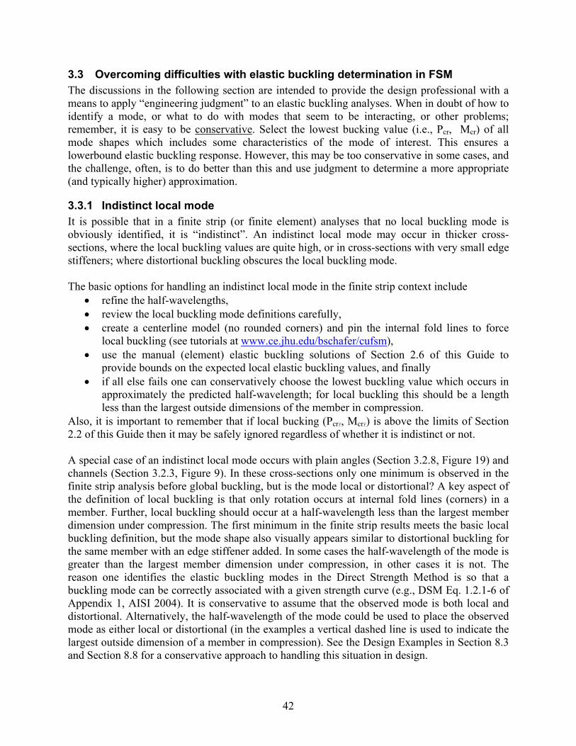
42
3.3 Overcoming difficulties with elastic buckling determination in FSM The discussions in the following section are intended to provide the design professional with a means to apply “engineering judgment” to an elastic buckling analyses. When in doubt of how to identify a mode, or what to do with modes that seem to be interacting, or other problems; remember, it is easy to be conservative. Select the lowest bucking value (i.e., Pcr, Mcr) of all mode shapes which includes some characteristics of the mode of interest. This ensures a lowerbound elastic buckling response. However, this may be too conservative in some cases, and the challenge, often, is to do better than this and use judgment to determine a more appropriate (and typically higher) approximation.
3.3.1 Indistinct local mode It is possible that in a finite strip (or finite element) analyses that no local buckling mode is obviously identified, it is “indistinct”. An indistinct local mode may occur in thicker cross-sections, where the local buckling values are quite high, or in cross-sections with very small edge stiffeners; where distortional buckling obscures the local buckling mode. The basic options for handling an indistinct local mode in the finite strip context include
• refine the half-wavelengths, • review the local buckling mode definitions carefully, • create a centerline model (no rounded corners) and pin the internal fold lines to force
local buckling (see tutorials at www.ce.jhu.edu/bschafer/cufsm), • use the manual (element) elastic buckling solutions of Section 2.6 of this Guide to
provide bounds on the expected local elastic buckling values, and finally • if all else fails one can conservatively choose the lowest buckling value which occurs in
approximately the predicted half-wavelength; for local buckling this should be a length less than the largest outside dimensions of the member in compression.
Also, it is important to remember that if local bucking (Pcrl, Mcrl) is above the limits of Section 2.2 of this Guide then it may be safely ignored regardless of whether it is indistinct or not. A special case of an indistinct local mode occurs with plain angles (Section 3.2.8, Figure 19) and channels (Section 3.2.3, Figure 9). In these cross-sections only one minimum is observed in the finite strip analysis before global buckling, but is the mode local or distortional? A key aspect of the definition of local buckling is that only rotation occurs at internal fold lines (corners) in a member. Further, local buckling should occur at a half-wavelength less than the largest member dimension under compression. The first minimum in the finite strip results meets the basic local buckling definition, but the mode shape also visually appears similar to distortional buckling for the same member with an edge stiffener added. In some cases the half-wavelength of the mode is greater than the largest member dimension under compression, in other cases it is not. The reason one identifies the elastic buckling modes in the Direct Strength Method is so that a buckling mode can be correctly associated with a given strength curve (e.g., DSM Eq. 1.2.1-6 of Appendix 1, AISI 2004). It is conservative to assume that the observed mode is both local and distortional. Alternatively, the half-wavelength of the mode could be used to place the observed mode as either local or distortional (in the examples a vertical dashed line is used to indicate the largest outside dimension of a member in compression). See the Design Examples in Section 8.3 and Section 8.8 for a conservative approach to handling this situation in design.
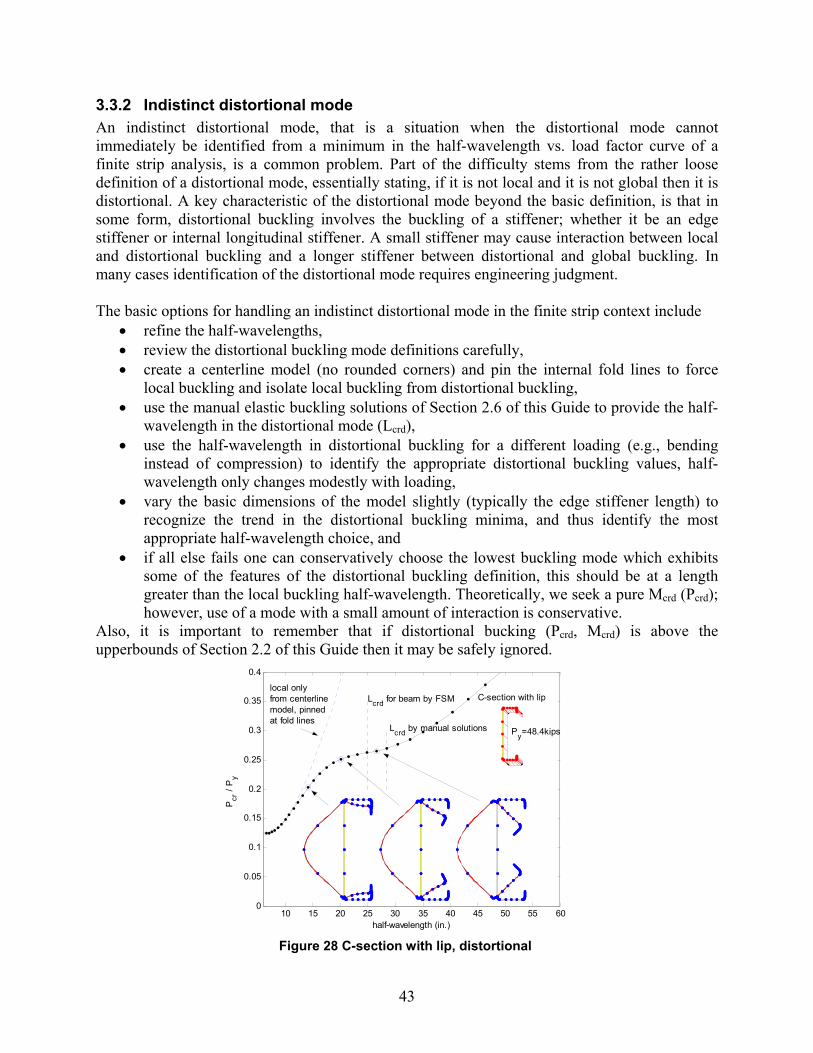
43
3.3.2 Indistinct distortional mode An indistinct distortional mode, that is a situation when the distortional mode cannot immediately be identified from a minimum in the half-wavelength vs. load factor curve of a finite strip analysis, is a common problem. Part of the difficulty stems from the rather loose definition of a distortional mode, essentially stating, if it is not local and it is not global then it is distortional. A key characteristic of the distortional mode beyond the basic definition, is that in some form, distortional buckling involves the buckling of a stiffener; whether it be an edge stiffener or internal longitudinal stiffener. A small stiffener may cause interaction between local and distortional buckling and a longer stiffener between distortional and global buckling. In many cases identification of the distortional mode requires engineering judgment. The basic options for handling an indistinct distortional mode in the finite strip context include
• refine the half-wavelengths, • review the distortional buckling mode definitions carefully, • create a centerline model (no rounded corners) and pin the internal fold lines to force
local buckling and isolate local buckling from distortional buckling, • use the manual elastic buckling solutions of Section 2.6 of this Guide to provide the half-
wavelength in the distortional mode (Lcrd), • use the half-wavelength in distortional buckling for a different loading (e.g., bending
instead of compression) to identify the appropriate distortional buckling values, half-wavelength only changes modestly with loading,
• vary the basic dimensions of the model slightly (typically the edge stiffener length) to recognize the trend in the distortional buckling minima, and thus identify the most appropriate half-wavelength choice, and
• if all else fails one can conservatively choose the lowest buckling mode which exhibits some of the features of the distortional buckling definition, this should be at a length greater than the local buckling half-wavelength. Theoretically, we seek a pure Mcrd (Pcrd); however, use of a mode with a small amount of interaction is conservative.
Also, it is important to remember that if distortional bucking (Pcrd, Mcrd) is above the upperbounds of Section 2.2 of this Guide then it may be safely ignored.
10 15 20 25 30 35 40 45 50 55 600
0.05
0.1
0.15
0.2
0.25
0.3
0.35
0.4
Lcrd by manual solutions
Lcrd for beam by FSM
half-wavelength (in.)
Pcr
/ P
y
C-section with lip
Py=48.4kips
local onlyfrom centerlinemodel, pinnedat fold lines
Figure 28 C-section with lip, distortional

44
C-section with lips: For the C-section with lips of Section 3.2.1, as shown in Figure 5b, the distortional mode in compression is indistinct. For cross-sections with wide webs and narrow flanges this is not an uncommon occurrence. The addition of a small web stiffener, which makes the web far more efficient also removes the problem of the indistinct distortional mode, see Section 3.2.2. Figure 28 provides a closer examination of the finite strip results for the C-section and applies many of the steps given above. For half-wavelengths around 15 in., the mode shape is a mixture of local and distortional buckling, note the bending in the flange. Further, when the analysis is restricted to local buckling only (dashed curve) the Pcr is essentially unchanged at a 15 in. half-wavelength, indicating this is not a pure distortional mode. The Direct Strength Method design expressions were calibrated to distortional buckling modes similar to those observed between half-wavelengths of 20 to 30 in. Through variation of the lip length (not shown) and by examination of the critical half-wavelength (Lcrd) from the manual elastic buckling solution and the beam solution (Figure 5a) the third of the three mode shapes identified in the inset of Figure 28 was selected as the distortional mode. Had either of the other modes shown been selected the engineer would have predicted on the conservative side. No justification exists for choosing a mode with a greater Lcrd than that of the manual solution (Chapter 9). Plain angle and channel: By some definition (primarily due to the half-wavelength), plain channels and plain tracks may be considered to have distortional modes. For the plain channel (track) of Section 3.2.3 and the plain angle of Section 3.2.8 see the discussion regarding indistinct local modes in the previous section (3.3.1).
Equal leg angle with lips: The equal leg angle with lips (Section 3.2.7) under bending, as given in Figure 17, has a distortional mode that is indistinct from the global (lateral-torsional) mode. In the strength calculations for a fully braced cross-section (Section 8.7) it is argued that this distortional mode would be restrained by the same bracing as the global mode. If this bracing is not present then the distortional mode would need to be considered in the calculation. At least two options exist (1) for the actual unbraced length visually inspect the mode shapes at half-wavelengths less than or equal to the unbraced length and assign Mcrd to the lowest mode which has distortional characteristics, (2) add artificial restrictions in the model to remove the torsional
100 101 102 1030
0.2
0.4
0.6
0.8
1
1.2
1.4
1.6
1.8
2
half-wavelength (in.)
Mcr
/ M
y
Angle with lips
My=16.85kip-in.
Distortional Mcr/My=0.57
supplementary analysis:vertical restraint added tosplit distortional fromlateral-torsional buckling.
original FSM results
Figure 29 Angle with lips, distortional
45
component from distortion. This second option was performed in Figure 29, where vertical movement in the bottom right corner of the cross-section was restricted, and a distinct distortional buckling mode is readily observed. The addition of artificial restraints to differentiate the modes does not lead to unconservative strength predictions. The purpose of the restraint is to help the engineer identify modes that are otherwise not immediately present in the analysis results. Completely ignoring a mode in a DSM calculation could lead to an unconservative strength prediction. So, determining a logical manner for including all the modes (when relevant) is important. Typically, the challenge is to identify the correct half-wavelength for selecting a given mode, and the addition of artificial restraints is often helpful in this regard. Once the proper half-wavelength is identified the elastic buckling value from the original analysis without artificial restraint at that half-wavelength may be used. In addition to the manual elastic buckling solutions of Chapter 9 the GBT methods discussed in Section 2.5 of this Guide can provide distortional buckling solutions for C’s and Z’s that eliminate the problem with indistinct distortional modes. Current research is investigating mechanics-based definitions that can uniquely identify distortional modes in the finite strip method (Schafer and Adany 2005). To date, such methods, including GBT, rely on the use of centerline models of the cross-section with sharp corners only.

46
3.3.3 Multiple local or distortional modes (stiffeners) As stiffeners are added to a cross-section it is possible to have more than two minima before global buckling occurs. The Direct Strength Method forces all such cases into one of two categories: local, or distortional. The C-section with lips that was modified with the addition of web stiffeners and a longer lip in Example 3.2.2 is shown again in Figure 30, this time compared with the unmodified cross-section (dashed curve). The first minima meets the local buckling definition, as only rotation is observed at internal fold lines. The second minima is similar to local buckling without the web stiffener, but the web stiffener itself undergoes distortional buckling. The question of whether this second minimum should be treated as local or distortional is somewhat irrelevant given that obvious local and distortional modes with lower buckling values exist. However, given the half-wavelength (relatively short) and the progression from the unmodified to the modified cross-section as shown in Figure 30, this second mode is best (though imperfectly) categorized as local buckling. The third minimum in the curve is the traditional distortional buckling mode. For complex cross-sections the keys to conservatively and reasonably assigning elastic buckling modes to a given class (local, distortional, or global) involve slightly more than the identification of minima in the finite strip analysis results. The mode shapes of the basic cross-section, without stiffeners, should be considered. In addition, the form of the Direct Strength expressions should also be considered. For a fully braced member distortional buckling gives lower strength than local buckling, but local buckling interacts with global modes, and thus for moderate to long unbraced lengths local-global interaction typically drives the solution. If a mode occurs at relatively short half-wavelengths, or is characteristic of local buckling of the basic cross-section, then the mode should likely be categorized as local, even if it fails the strict definition of rotation only at the internal folds of the member.
100 101 1020
0.2
0.4
0.6
0.8
1
1.2
1.4
1.6
1.8
2
half-wavelength (in.)
Mcr
/ M
y
C-section with lips modified
Mcr/My=1.40 Mcr/My=1.50 Mcr/My=0.98
before
after
local bucklingimproved, but 'split' by webstiffeners
dist. bucklingimproved byincreased lip
(a) (b) (c)
Figure 30 Modifed C-section multiple modes
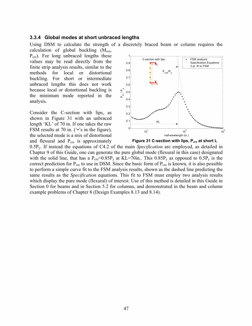
47
3.3.4 Global modes at short unbraced lengths Using DSM to calculate the strength of a discretely braced beam or column requires the calculation of global buckling (Mcre, Pcre). For long unbraced lengths these values may be read directly from the finite strip analysis results, similar to the methods for local or distortional buckling. For short or intermediate unbraced lengths this does not work because local or distortional buckling is the minimum mode reported in the analysis. Consider the C-section with lips, as shown in Figure 31 with an unbraced length ‘KL’ of 70 in. If one takes the raw FSM results at 70 in. (‘•’s in the figure), the selected mode is a mix of distortional and flexural and Pcre is approximately 0.5Py. If instead the equations of C4.2 of the main Specification are employed, as detailed in Chapter 9 of this Guide, one can generate the pure global mode (flexural in this case) designated with the solid line, that has a Pcre=0.85Py at KL=70in.. This 0.85Py as opposed to 0.5Py is the correct prediction for Pcre to use in DSM. Since the basic form of Pcre is known, it is also possible to perform a simple curve fit to the FSM analysis results, shown as the dashed line predicting the same results as the Specification equations. This fit to FSM must employ two analysis results which display the pure mode (flexural) of interest. Use of this method is detailed in this Guide in Section 0 for beams and in Section 5.2 for columns, and demonstrated in the beam and column example problems of Chapter 8 (Design Examples 8.13 and 8.14).
101 102 1030
0.1
0.2
0.3
0.4
0.5
0.6
0.7
0.8
0.9
1
half-wavelength (in.)
Pcr
/ P
y
FSM analysisSpecification Equations2 pt. fit to FSM
C-section with lips
KL
Pcre/Py
Figure 31 C-section with lips, Pcre at short L
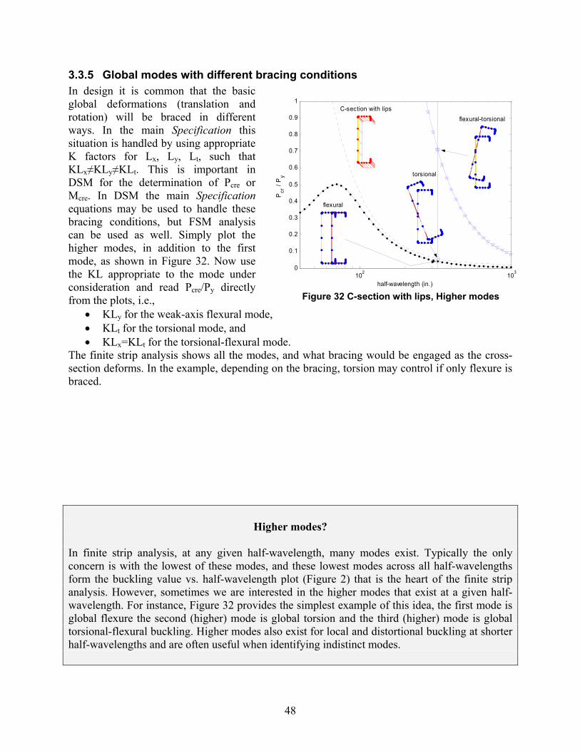
48
3.3.5 Global modes with different bracing conditions In design it is common that the basic global deformations (translation and rotation) will be braced in different ways. In the main Specification this situation is handled by using appropriate K factors for Lx, Ly, Lt, such that KLx≠KLy≠KLt. This is important in DSM for the determination of Pcre or Mcre. In DSM the main Specification equations may be used to handle these bracing conditions, but FSM analysis can be used as well. Simply plot the higher modes, in addition to the first mode, as shown in Figure 32. Now use the KL appropriate to the mode under consideration and read Pcre/Py directly from the plots, i.e.,
• KLy for the weak-axis flexural mode, • KLt for the torsional mode, and • KLx=KLt for the torsional-flexural mode.
The finite strip analysis shows all the modes, and what bracing would be engaged as the cross-section deforms. In the example, depending on the bracing, torsion may control if only flexure is braced.
Higher modes? In finite strip analysis, at any given half-wavelength, many modes exist. Typically the only concern is with the lowest of these modes, and these lowest modes across all half-wavelengths form the buckling value vs. half-wavelength plot (Figure 2) that is the heart of the finite strip analysis. However, sometimes we are interested in the higher modes that exist at a given half-wavelength. For instance, Figure 32 provides the simplest example of this idea, the first mode is global flexure the second (higher) mode is global torsion and the third (higher) mode is global torsional-flexural buckling. Higher modes also exist for local and distortional buckling at shorter half-wavelengths and are often useful when identifying indistinct modes.
102 1030
0.1
0.2
0.3
0.4
0.5
0.6
0.7
0.8
0.9
1
half-wavelength (in.)P
cr /
Py
C-section with lips
flexural
torsional
flexural-torsional
Figure 32 C-section with lips, Higher modes

49
3.3.6 Influence of moment gradient For beams, local, distortional, and global buckling (Mcrl, Mcrd, Mcre) are all potentially influenced by moment gradient. As calculated in a finite strip analysis, moment is assumed uniform. A general purpose finite element analysis (Section 2.4) could include moment gradient; for FSM the following advice is given: Local buckling: ignore moment gradient, unless the moment changes markedly inside the short half-wavelength of a local mode, then the anticipated increase for this mode is small. Distortional buckling: research (Yu 2005) indicates that moderate increases (30% or less) in the distortional buckling moment Mcrd occur due to moment gradient. General purpose finite element analysis (Section 2.4) provides a rational analysis means to account for this increase. Ignoring the moment gradient is conservative. Global (lateral-torsional) buckling: moment gradient may be accounted for using the Cb factor (Eq. C3.1.2.1-10) of the main Specification. Actual Mcre, accounting for moment gradient, is equal to CbM*
cre where M*cre is the result directly from the finite strip analysis or appropriate
closed-form formula as shown in Chapter 9 of this Guide.
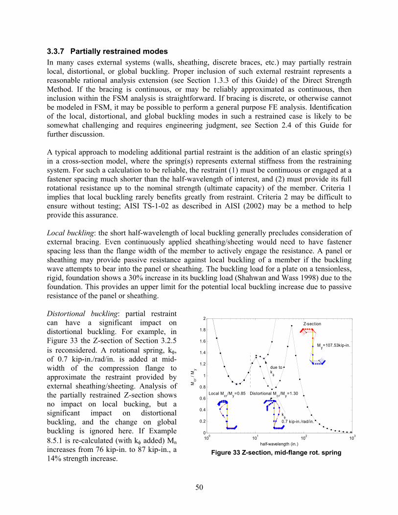
50
3.3.7 Partially restrained modes In many cases external systems (walls, sheathing, discrete braces, etc.) may partially restrain local, distortional, or global buckling. Proper inclusion of such external restraint represents a reasonable rational analysis extension (see Section 1.3.3 of this Guide) of the Direct Strength Method. If the bracing is continuous, or may be reliably approximated as continuous, then inclusion within the FSM analysis is straightforward. If bracing is discrete, or otherwise cannot be modeled in FSM, it may be possible to perform a general purpose FE analysis. Identification of the local, distortional, and global buckling modes in such a restrained case is likely to be somewhat challenging and requires engineering judgment, see Section 2.4 of this Guide for further discussion. A typical approach to modeling additional partial restraint is the addition of an elastic spring(s) in a cross-section model, where the spring(s) represents external stiffness from the restraining system. For such a calculation to be reliable, the restraint (1) must be continuous or engaged at a fastener spacing much shorter than the half-wavelength of interest, and (2) must provide its full rotational resistance up to the nominal strength (ultimate capacity) of the member. Criteria 1 implies that local buckling rarely benefits greatly from restraint. Criteria 2 may be difficult to ensure without testing; AISI TS-1-02 as described in AISI (2002) may be a method to help provide this assurance. Local buckling: the short half-wavelength of local buckling generally precludes consideration of external bracing. Even continuously applied sheathing/sheeting would need to have fastener spacing less than the flange width of the member to actively engage the resistance. A panel or sheathing may provide passive resistance against local buckling of a member if the buckling wave attempts to bear into the panel or sheathing. The buckling load for a plate on a tensionless, rigid, foundation shows a 30% increase in its buckling load (Shahwan and Wass 1998) due to the foundation. This provides an upper limit for the potential local buckling increase due to passive resistance of the panel or sheathing. Distortional buckling: partial restraint can have a significant impact on distortional buckling. For example, in Figure 33 the Z-section of Section 3.2.5 is reconsidered. A rotational spring, kφ, of 0.7 kip-in./rad/in. is added at mid-width of the compression flange to approximate the restraint provided by external sheathing/sheeting. Analysis of the partially restrained Z-section shows no impact on local bucking, but a significant impact on distortional buckling, and the change on global buckling is ignored here. If Example 8.5.1 is re-calculated (with kφ added) Mn increases from 76 kip-in. to 87 kip-in., a 14% strength increase.
Z-section (AISI 2002 Ex. I-10)
My=107.53kip-in.
Local Mcr/My=0.85Distortional Mcr/My=0.77
Lateral-torsional
100 101 102 1030
0.2
0.4
0.6
0.8
1
1.2
1.4
1.6
1.8
2
half-wavelength (in.)
Mcr
/ M
y
Z-section
My=107.53kip-in.
Local Mcr/My=0.85 Distortional Mcr/My=1.30
due tokφ
kφ
0.7 kip-in./rad/in.
Figure 33 Z-section, mid-flange rot. spring
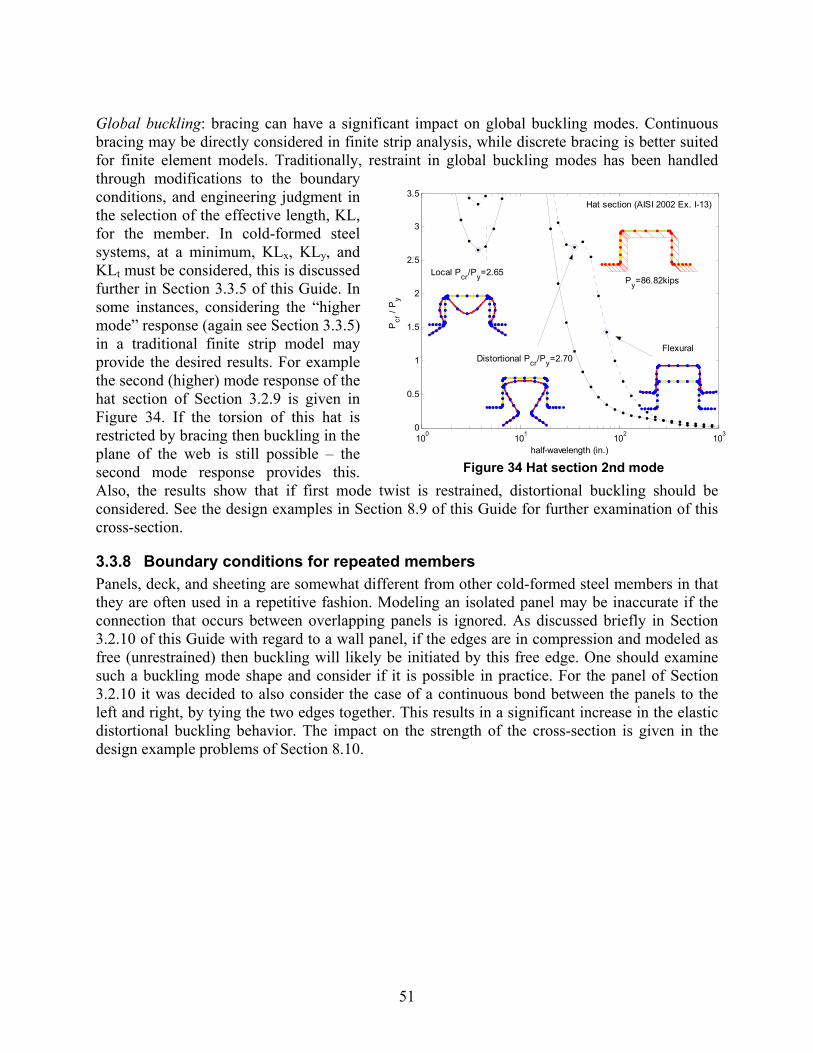
51
Global buckling: bracing can have a significant impact on global buckling modes. Continuous bracing may be directly considered in finite strip analysis, while discrete bracing is better suited for finite element models. Traditionally, restraint in global buckling modes has been handled through modifications to the boundary conditions, and engineering judgment in the selection of the effective length, KL, for the member. In cold-formed steel systems, at a minimum, KLx, KLy, and KLt must be considered, this is discussed further in Section 3.3.5 of this Guide. In some instances, considering the “higher mode” response (again see Section 3.3.5) in a traditional finite strip model may provide the desired results. For example the second (higher) mode response of the hat section of Section 3.2.9 is given in Figure 34. If the torsion of this hat is restricted by bracing then buckling in the plane of the web is still possible – the second mode response provides this. Also, the results show that if first mode twist is restrained, distortional buckling should be considered. See the design examples in Section 8.9 of this Guide for further examination of this cross-section.
3.3.8 Boundary conditions for repeated members Panels, deck, and sheeting are somewhat different from other cold-formed steel members in that they are often used in a repetitive fashion. Modeling an isolated panel may be inaccurate if the connection that occurs between overlapping panels is ignored. As discussed briefly in Section 3.2.10 of this Guide with regard to a wall panel, if the edges are in compression and modeled as free (unrestrained) then buckling will likely be initiated by this free edge. One should examine such a buckling mode shape and consider if it is possible in practice. For the panel of Section 3.2.10 it was decided to also consider the case of a continuous bond between the panels to the left and right, by tying the two edges together. This results in a significant increase in the elastic distortional buckling behavior. The impact on the strength of the cross-section is given in the design example problems of Section 8.10.
100 101 102 1030
0.5
1
1.5
2
2.5
3
3.5
half-wavelength (in.)
Pcr
/ P
y
Hat section (AISI 2002 Ex. I-13)
Py=86.82kipsLocal Pcr/Py=2.65
Distortional Pcr/Py=2.70Flexural
Figure 34 Hat section 2nd mode

52
3.3.9 Members with holes Research extending the Direct Strength Method to members with holes is currently active. The next update to the Direct Strength Method will include explicit provisions for handling holes. The main Specification provisions do provide some guidance that is readily useable: in particular, when holes may be safely ignored in the strength calculation. Ignoring holes for bending members: bending members with holes in the web are addressed in the main Specification in Section B2.4. Within a specific set of dimensional limits (given in B2.4), web openings may be ignored. In particular, if a mid-depth web opening is less than 38% of the web depth itself then the hole does not impact the strength. A rational extension of this finding to the Direct Strength Method is that holes do not need to be considered in calculating Mcrl, Mcrd, Mcre if they meet the limits in main Specification B2.4. Ignoring holes for compression members: compression members with holes in the web are addressed in the main Specification in Section B2.2. This section is applicable to widely spaced circular holes – and the hole must be less than 50% of the depth, other dimensional limits are listed in B2.2. If the element with the hole present is stocky ( 6730.FF cry ≤ , where Fcr is the buckling stress of the element ignoring the hole and Fy is the yield stress) the remaining element portion is assumed to take the full yield stress. Effectively, this limits the nominal strength to AnetFy = Py net as opposed to AgrossFy = Py. In the Direct Strength Method this criteria can be rationally extended to the cross-section: if the web hole meets the geometric criteria of main Specification Section B2.2 and Pcrl > 2.21Py (where Pcrl ignores the hole) then determine the nominal strength of the cross-section following the Direct Strength Method criteria of Section 1.2.1 (AISI 2004), but replace Py with Py net and ignore the hole in calculation of Pcrl, Pcrd, Pcre. Rational analysis for handling holes: Currently, for other situations, rational analysis extensions to DSM are the only alternative. For example, elastic buckling (Pcrl, Pcrd, Pcre, Mcrl, Mcrd, Mcre) of members with holes can be determined by general-purpose finite element analysis (Section 2.4). For example, Sarawit (2004) studied rack post cross-sections with patterned holes. He performed finite element analysis of members comprised of shell elements with the holes explicitly modeled to determine the impact of the holes on local, distortional, and global buckling. This is a time consuming process and careful visual inspection of the resulting mode shapes is required to assign local, distortional, and global buckling modes. Take care with weighted thickness: Another engineering approach to handling holes in members is to use a weighted average thickness at the hole location. Take care with this approach, it may not accurately capture the rigidity of the cross-section in the different buckling modes - and thus produce poor results. The weighted thickness is length dependent so different weights would be required for every half-wavelength examined in a finite strip analysis. Take care with net section: Another engineering approach to handling holes is to model the cross-section at the net section only. Thus, the model of a C-section with a web hole would simply model the flange and the portion of the web above the hole. Such a model can lead to artificially high predictions of the local buckling stress. In the actual member, even with a hole, the center of the web may trigger the instability since longitudinal continuity exists, but in a net section model the center cannot cause the instability and the resulting buckling stress may be artificially elevated.
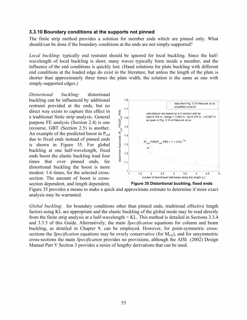
53
3.3.10 Boundary conditions at the supports not pinned The finite strip method provides a solution for member ends which are pinned only. What should/can be done if the boundary conditions at the ends are not simply-supported? Local buckling: typically end restraint should be ignored for local buckling. Since the half-wavelength of local buckling is short, many waves typically form inside a member, and the influence of the end conditions is quickly lost. (Hand solutions for plate buckling with different end conditions at the loaded edge do exist in the literature, but unless the length of the plate is shorter than approximately three times the plate width, the solution is the same as one with simply-supported edges.) Distortional buckling: distortional buckling can be influenced by additional restraint provided at the ends, but no direct way exists to capture this effect in a traditional finite strip analysis. General purpose FE analysis (Section 2.4) is one recourse, GBT (Section 2.5) is another. An example of the predicted boost in Pcrd due to fixed ends instead of pinned ends is shown in Figure 35. For global buckling at one half-wavelength, fixed ends boost the elastic buckling load four times that over pinned ends, for distortional buckling the boost is more modest: 1.6 times, for the selected cross-section. The amount of boost is cross-section dependent, and length dependent, Figure 35 provides a means to make a quick and approximate estimate to determine if more exact analysis may be warranted. Global buckling: for boundary conditions other than pinned ends, traditional effective length factors using KL are appropriate and the elastic buckling of the global mode may be read directly from the finite strip analysis at a half-wavelength = KL. This method is detailed in Sections 3.3.4 and 3.3.5 of this Guide. Alternatively, the main Specification equations for column and beam buckling, as detailed in Chapter 9, can be employed. However, for point-symmetric cross-sections the Specification equations may be overly conservative (for Mcre), and for unsymmetric cross-sections the main Specification provides no provisions, although the AISI (2002) Design Manual Part V Section 3 provides a series of lengthy derivations that can be used.
1 1.5 2 2.5 3 3.5 4 4.5 51
1.1
1.2
1.3
1.4
1.5
1.6
1.7
1.8
number of distortional half-waves along the length (λ)
boos
t fro
m fi
xed
ends
: (P cr
d FIX
)/(P cr
d PIN
)
(Pcrd FIX)/(Pcrd PIN) = 1 + 0.6/λ1.5
data from Fig. 3.10 Hancock et al.simplified curve fit
calculations are based on a C-section with lipweb=4.724 in., flange = 3.543 in., lip=0.275 in., t=0.047 in.as given in Fig. 3.10 of Hancock et al.
Figure 35 Distortional buckling, fixed ends
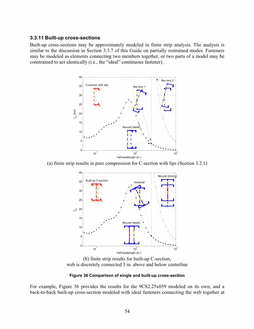
54
3.3.11 Built-up cross-sections Built-up cross-sections may be approximately modeled in finite strip analysis. The analysis is similar to the discussion in Section 3.3.7 of this Guide on partially restrained modes. Fasteners may be modeled as elements connecting two members together, or two parts of a model may be constrained to act identically (i.e., the “ideal” continuous fastener).
101 102 1030
5
10
15
20
25
30
35
40
half-wavelength (in.)
f cr (k
si)
C-section with lips
flexural (weak)
flex-tors 1
flex-tors 2
(a) finite strip results in pure compression for C-section with lips (Section 3.2.1)
101 102 1030
5
10
15
20
25
30
35
40
half-wavelength (in.)
f cr
Built-up C-section
flexural (weak)
torsional
flexural (strong)
(b) finite strip results for built-up C-section,
web is discretely connected 3 in. above and below centerline
Figure 36 Comparison of single and built-up cross-section For example, Figure 36 provides the results for the 9CS2.25x059 modeled on its own, and a back-to-back built-up cross-section modeled with ideal fasteners connecting the web together at

55
two points, 3 in. above and below centerline. This is an upperbound model, because the connection is (a) continuous and (b) axial and shear are both connected. This built-up cross-section is motivated from AISI (2002) Design Manual Example II-8 which is discussed further in Chapter 5. The results have been plotted in terms of stress so that the two cross-sections may be most readily compared to one another. The buckling stress for local and distortional buckling are unaffected by connecting the two cross-sections together. Thus, Pcrl, Pcrd are simply twice the single cross-section value in the built-up cross-section. However, in the built-up cross-section the weak-axis flexural mode is increased, and the torsional-flexural mode is replaced by a separate torsion mode and strong-axis flexure mode. If weak-axis flexure is adequately braced, then these modes become the potential Pcre modes of interest. (Note, if the fasteners cannot provide the shear resistance then the torsional-flexural mode will still occur). Note, a toe-to-toe built-up C-section will have a different behavior than the back-to-back cross-section. Most noticeably, the distortional buckling (Pcrd or Mcrd) will be elevated greater than just two times a single C-section response. Torsional-flexural buckling will also be greatly increased due to the enhanced torsional stiffness of the closed cross-section shape.
56
4 Beam design
This chapter begins with the application of the Direct Strength Method to fully braced beams. To illustrate the influence of unbraced length on bending strength solutions are provided for generating a beam chart in Section 4.2. This is followed by Section 4.3 which focuses on serviceability calculations using the Direct Strength Method. Section 4.4 addresses shear, web crippling, and interaction checks – which are largely outside the scope of the Direct Strength Method and require using the main Specification in conjunction with the Direct Strength Method. Finally, in Section 4.5, the beam design examples from the AISI (2002) Design Manual are considered and updated for use with the Direct Strength Method. Issues of interest that arise in these examples include the use of Cb, R for uplift, and cold work of forming. Chapter 8 provides Direct Strength Method beam design examples for the 12 different cross-sections of Section 3.2.
4.1 Beam design for fully braced beams In the main Specification it is common to consider the nominal strength of a fully braced beam and determine the effective section modulus for this case (i.e., Mn=SeFy). This provides the most conservative approximation of the effective properties, and Chapter 1 of the AISI (2002) Design Manual provides extensive coverage of this calculation. The nominal strength of a fully braced member in the Direct Strength Method can be readily found by setting the global buckling capacity to its full nominal strength, the yield moment (i.e., Mne=My of DSM Section 1.2.2.1), and then proceed normally through the Direct Strength Method expressions. Thus, the definition of a fully braced beam assumes that the bracing precludes global modes, but leaves local and distortional buckling free to form. Examination of the buckling mode shapes themselves can help in determining the impact that bracing may have. The bending strength for fully braced beams is provided for all the cross-sections of Section 3.2 in Chapter 8, Examples 8.1 through 8.12. For general beam design (not fully braced) the primary difference is that lateral-torsional buckling must now be considered (Mcre < 2.78My implying Mne < My) and therefore the local buckling strength (Mnl) will be reduced. In addition, shear, web crippling, and interaction of bending + shear, and bending + crippling, must also be considered. These issues are discussed further in the following sections.
Fully braced? Fully braced. A cross-section that is braced such that global buckling is restrained. The term fully braced is used extensively in the discussion and Design Examples of this Guide. This is largely due to a desire to compare Direct Strength Method results to the effective property calculations used in the main Specification (e.g., see Part I of AISI (2002)). A key difference between the main Specification and the Direct Strength Method that influences this comparison is that DSM includes the possibility of distortional buckling when a member is fully braced.
57
4.2 Beam charts, local, distortional, and global buckling as a function of length One of the main advantages of DSM is the ability to examine cross-section variations with efficiency. Whether you are a product designer, or a consulting engineer, beam charts which provide the nominal strength of a given beam vs. length are often useful in design. To produce a beam chart with DSM correctly it is important to understand the unique influence of unbraced length on each of the buckling classes: local, distortional, and global. For creating the beam chart My, Mcrl(L), Mcrd(L), Mcre(L) where (L) indicates the quantity as a function of length is required. Local buckling occurs at short half-wavelengths, thus in longer members it merely repeats itself many times along the length. Once the length of the member is greater than the depth (or largest dimension) of the cross-section little if any change occurs in the local buckling value. Given this behavior it is prudent to assume that
Mcrl(L) = Mcrl , i.e., local buckling remains unchanged for any length. Distortional buckling occurs at an intermediate half-wavelength and an unbraced length shorter than the distortional buckling half-wavelength length is possible. In limited cases one can read a distortional buckling value at L less than the distortional buckling minimum point directly from the finite strip analysis results. Alternatively, a shortened length may be substituted directly in the closed-formed distortional buckling formulas provided in Chapter 9 of this Guide. The simplest procedure is to use an approximation based on the work of Yu (2005):
( ) ( ) ( )crdLLlncrd
*crdcrdcrd LLMLLM =< , and
( ) *crdcrdcrd MLLM =≥ ,
where L is the length of interest, Lcrd is the half-wavelength at which the distortional buckling moment is a minimum (e.g., in a finite strip analysis) and M*
crd is the distortional buckling moment at the minimum point. The equations above are accurate for a wide range of C- and Z-sections (Yu 2005) and are recommended for application for any cold-formed steel cross-section. Global (lateral-torsional) buckling occurs at long lengths. To determine Mcre(L) two options are available: (1) use the closed-form expression in the main Specification as illustrated in Section 2.6 of this Guide, or (2) recognize the form of Mcre as a function of L and fit an appropriate expression to the generated finite strip data (see Section 3.3.4 of this Guide for further discussion). Method (2) does not require the calculation of cross-section properties and is relatively easily implemented. The form of Mcre as a function of L is known:
( ) ( )422cre L1L1M β+α=
To find α and β pick any two pairs of points in the finite strip analysis curve at half-wavelengths long enough that the mode shapes display the lateral-torsional mode. Defining such pairs as (Lcr1,Mcre1) and (Lcr2,Mcre2), then α and β are:
22cr
21cr
42cr
22cre
41cr
21cre
LLLMLM
−
−=α 2
1cr2
2cr
22cr
21cr
22cr
22cre
21cr
21cre
LLLL)LMLM(
−
−=β
Following this methodology a beam chart is developed for the C-section with lips, of Section 3.2.1. The complete development of the chart is given in Section 8.13 of this Guide. The final chart is provided in Figure 37(a)and(b). Additional charts for the Z-section with lips are provided in parts (c) and (d) of this figure.

58
0 5 10 15 200
20
40
60
80
100
120
140
length (ft)
bend
ing
capa
city
(kip
-in.)
M n L( )
M ne L( )
M nl L( )
M nd L( )
L
12
Mne
Mnd
0 5 10 15 200
20
40
60
80
100
120
140
length (ft)
bend
ing
capa
city
(kip
-in.)
M n L( )
M n2 L( )
L
12
9CS2.5x059 modified
9CS2.5x059
(a) Mn for C-section with lips
(see Sections 3.2.1, 8.1 and 8.13) (b) Mn for C-section with lips and modified
(see Sections 3.2.2, 8.2 and 8.13)
0 5 10 15 200
20
40
60
80
100
120
length (ft)
bend
ing
capa
city
(kip
-in.)
Mn L( )
Mne L( )
Mnl L( )
Mnd L( )
L
12
Mne
Mnl
Mnd
0 5 10 15 20
0
20
40
60
80
100
120
length (ft)
bend
ing
capa
city
(kip
-in.)
M n L( )
M n2 L( )
L
12
8ZS2.25x059 modified
8ZS2.25x059
(c) Mn for Z-section with lips (see Sections 3.2.5 and 8.5)
(d) Mn for Z-section with lips and modified (see Sections 3.2.6 and 8.6)
Figure 37 Beam charts for C- and Z-sections with lips by the Direct Strength Method Figure 37(a) and (c) show how the three Direct Strength prediction equations behave as a function of length: Mnl is reduced from Mne, unless Mne is low enough at which length Mnl and Mne converge. Mnd is a separate strength check that is independent of length for intermediate to large lengths, and may control the strength over a relatively short regime of unbraced length. The modified cross-sections provide improved performance over the original cross-sections.
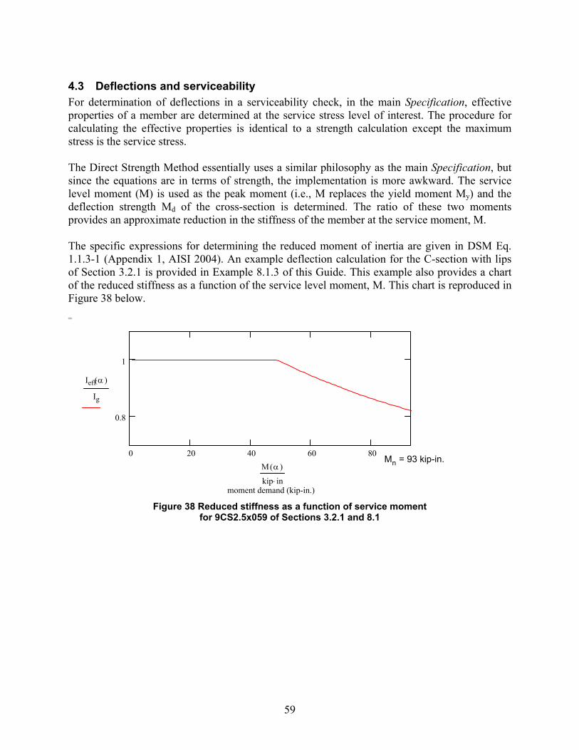
59
4.3 Deflections and serviceability For determination of deflections in a serviceability check, in the main Specification, effective properties of a member are determined at the service stress level of interest. The procedure for calculating the effective properties is identical to a strength calculation except the maximum stress is the service stress. The Direct Strength Method essentially uses a similar philosophy as the main Specification, but since the equations are in terms of strength, the implementation is more awkward. The service level moment (M) is used as the peak moment (i.e., M replaces the yield moment My) and the deflection strength Md of the cross-section is determined. The ratio of these two moments provides an approximate reduction in the stiffness of the member at the service moment, M. The specific expressions for determining the reduced moment of inertia are given in DSM Eq. 1.1.3-1 (Appendix 1, AISI 2004). An example deflection calculation for the C-section with lips of Section 3.2.1 is provided in Example 8.1.3 of this Guide. This example also provides a chart of the reduced stiffness as a function of the service level moment, M. This chart is reproduced in Figure 38 below.
0 20 40 60 80
0.8
1
moment demand (kip-in.)
Ieff α( )
Ig
M α( )
kip in⋅
Mn = 93 kip-in.
Figure 38 Reduced stiffness as a function of service moment
for 9CS2.5x059 of Sections 3.2.1 and 8.1
60
4.4 Combining DSM and the main Specification for beams While DSM does provide a general methodology for prediction of the nominal flexural strength, Mn, strength in shear, and web crippling are not covered. As a result, the main Specification is required for shear, and web crippling calculations when applicable.
4.4.1 Shear The provisions for shear are in main Specification Section C3.2. For members with flat webs these provisions can be used without modification. For members which do not have flat webs no guidance is provided in the Specification. As a rational analysis extension the existing C3.2.1 equations are recast into the Direct Strength format and are suggested for use:
for 8150.v ≤λ
yn VV = for 23118150 .. v ≤λ<
ycrn VV.V 8150=
for 2311.v >λ
crn VV =
where cryv VV=λ
ywy F.AV 600= Vcr = critical elastic shear buckling force
For members with flat webs these expressions yield the same results as the existing main Specification Section C3.2. As a rational analysis extension, φ=0.8, and Ω=2.0 per A1.1(b) of the main Specification. Vcr could be determined by FE analysis (Section 2.4) or other methods. Holes: For shear in members with holes main Specification C3.2.2 provides a method for members meeting given geometric limits. For further information on members with holes see Section 3.3.9 of this Guide.
4.4.2 Combined bending and shear The main Specification provisions of C3.3 provide a means to consider combined bending and shear. As detailed in Table 1, Mn calculated by the Direct Strength Method may be used in C3.3.
4.4.3 Web crippling Web crippling is covered in C3.4 of the main Specification. The provisions are empirically derived from experimental data, so rational analysis extensions without testing are difficult. Basic geometric limits for the applicability of the provisions to I, C, Z, hat, and deck cross-sections are provided. For other cross-sections strength must be determined by rational analysis or testing (section A1.1 of the main Specification).
61
4.5 Notes on example problems from AISI (2002) Design Manual The AISI (2002) Design Manual includes six beam design examples. Those examples are used as the basis for the beam examples provided in this Guide (Chapter 8). To aid the reader in completing a comparison of the traditional main Specification methods to DSM, Table 2 was prepared. Within the design examples of this Guide additional commentary comparing the main Specification approach with DSM is provided.
Table 2 Comparison of beam examples between the AISI (2002) Design Manual and this Guide
AISI (2002) Design Manual Example DSM Design Guide Example II-1 Four Span Continuous C-Purlins Attached to
Through Fastened Roof – LRFD Section 8.1 Design Examples 8.1.1 - 8.1.3
II-2 Four Span Continuous Z-Purlins Attached to Through Fastened Roof – ASD
Section 8.5 Design Examples 8.5.1 and 8.5.2
II-3 C-Section Without Lips Braced at Mid-span Section 8.3 Design Examples 8.3.1 and 8.3.2 II-4 Fully Braced Hat Section Section 8.9 Design Example 8.9.1 II-5 Tubular Section – Round Not covered by the Direct Strength Method1 II-6 C-Section with Openings Not covered in this Guide2 1 This cross-section is not covered by the Direct Strength Method, main Specification rules apply.
2 No design example is provided in this Guide; however two items worthy of discussion are provided here. (a) Cold work of forming: AISI (2002) Example II-6 uses the cold work of forming provisions of A7.2 of the main Specification. Main Specification Section A7.2 states that ρ for all effective width calculations must equal one when calculated at the average, elevated, yield stress Fy = Fya. In the Direct Strength Method ρ is not used, instead the ρ = 1 check is equivalent to ensuring Mnl = My at Fy = Fya, and Mnd = My at Fy=Fya. Cross-sections which meet this criteria are eligible for inclusion of cold work of forming and use of Fy=Fya in DSM. (b) Bending (with holes): For the example cross-section do/h = 1.5/3.643 = 0.412 > 0.38, therefore the hole may not be ignored in the calculation. Since the hole may not be ignored simple rational analysis extension of the Direct Strength Method becomes complicated. The AISI (2002) Design Example proceeds by calculating the effective section for the remaining lip above the hole – this stress (Fcr in the AISI (2002) Example II-6) could be used to approximate Mcrl in the Direct Strength Method, but a similar calculation for Mcrd is not immediately available, see Section 3.3.9 of this Guide for further discussion.
62
5 Column design
This chapter begins with a discussion of the strength determination of braced columns. Although it is somewhat artificial to divorce columns from beam-columns this Chapter covers only concentrically loaded columns, and leaves beam-columns to Chapter 6. To illustrate the influence of unbraced length on compressive strength, solutions are provided for generating a column chart in Section 5.2. In Section 5.3, the design examples from Part III of the AISI (2002) Design Manual are considered and updated for use with the Direct Strength Method. Part III of the Manual addresses both columns and beam-columns; in this Chapter only the column calculations will be considered. Issues of interest that arise in these examples include bracing boundary conditions and constrained buckling.
5.1 Column design for continuously braced columns In the main Specification it is common to consider the nominal strength of a braced column and determine the effective area for this case (i.e., Pn=AeFy). This provides the most conservative approximation of the effective area, and Chapter 1 of the AISI (2002) Design Manual provides extensive coverage of this calculation. The nominal strength of a fully braced member in the Direct Strength Method can be readily found by setting the global buckling capacity to its full nominal strength, the squash load (i.e., Pne=Py of DSM Section 1.2.1.1), and then proceeding normally through the Direct Strength Method expressions. Thus, the definition of a fully braced column assumes that the bracing precludes global modes, but leaves local and distortional buckling free to form. Examination of the buckling mode shapes themselves can help in determining the impact that bracing may have. The compressive strength for braced columns is provided for all the cross-sections of Section 3.2 in Chapter 8, Examples 8.1 through 8.12. For general column design (not fully braced) the primary difference is that flexural, or torsional-flexural buckling must now be considered and therefore the local buckling strength (Pnl) will be reduced. These issues are discussed further in the following sections.

63
5.2 Creating column charts Creation of a column chart is similar to that of a beam chart (Section 4.1). The key consideration is to understand the unique influence that the unbraced length has on each of the buckling classes: local, distortional, and global. For creating a column chart Py, Pcrl(L), Pcrd(L), Pcre(L), where (L) indicates quantity as a function of length, is required. Local buckling occurs at short half-wavelengths, thus in longer members it merely repeats itself many times along the length. Once the length of the member is greater than the depth (or largest dimension) of the cross-section, little if any change occurs in the local buckling value. Given this behavior it is prudent to assume that
Pcrl(L) = Pcrl , i.e., local buckling remains unchanged for any length. Distortional buckling occurs at an intermediate half-wavelength and an unbraced length shorter than the distortional buckling half-wavelength length is possible. In limited cases one can determine a distortional buckling value at L less than the distortional buckling minimum point directly from the finite strip analysis results. Alternatively, a shortened length may be substituted directly in the closed-formed distortional buckling formulas detailed in Chapter 9 of this Guide. The simplest procedure is to use an approximation based on the work of Yu (2005):
( ) ( ) ( )crdLLlncrd
*crdcrdcrd LLPLLP =< , and
( ) *crdcrdcrd PLLP =≥ ,
where L is the length of interest, Lcrd is the half-wavelength at which the distortional buckling load is a minimum (e.g., in a finite strip analysis) and P*
crd is the distortional buckling load at the minimum point. This approximate expressions was derived for C- and Z-sections (Yu 2005) but it accurate enough for general applicability. Global (flexural, torsional-flexural) buckling occurs at long lengths. To determine Pcre(L) two options are available: (1) use the closed-form expression in the main Specification Section C4.1-C4.4 as illustrated in Chapter 9, or (2) recognize the form of Pcre as a function of L and fit an appropriate expression to the generated finite strip data (see Section 3.3.4 for further discussion). Method (2) has the advantage in that it does not require the calculation of cross-section properties and is relatively easily implemented. The form of Pcre as a function of L is known:
( ) ( )422cre L1L1P β+α=
To find α and β which can be determined by picking any two pairs of points in the finite strip analysis curve at lengths long enough that clearly display the flexural or torsional-flexural mode of interest, namely if we define the pairs (Lcr1,Pcre1) and (Lcr2,Pcre2), then α and β are:
22cr
21cr
42cr
22cre
41cr
21cre
LLLPLP
−−
=α 21cr
22cr
22cr
21cr
22cr
22cre
21cr
21cre
LLLL)LPLP(
−−
=β
Columns may display different buckling modes at long lengths (e.g., switching from torsional-flexural to flexure) it is important that the two selected points be consistent with the buckling mode of interest. Further, it may be desirable to determine curves for more than one mode – i.e., for both weak-axis flexure, and for torsional-flexural buckling.

64
Following this methodology a column chart was developed for the C-section with lips of Section 3.2.1. The complete development of the chart is given in Section 8.14 of this Guide. The final chart is provided in Figure 39.
0 5 10 15 200
10
20
30
40
50
length (ft)
com
pres
sion
cap
acity
(kip
)
Pn L( )
Pne L( )
Pnl L( )
Pnd L( )
L
12
Pne
Pnd
Pnl
0 5 10 15 200
5
10
15
20
25
30
35
40
45
50
55
length (ft)
com
pres
sion
cap
acity
(kip
)
Pn L( )
Pn2 L( )
Pnd2 L( )
Pne2 L( )
L
12
9CS2.5x059modified
9CS2.5x059
(a) Pn for C-section with lips
(see Sections 3.2.1, 8.1, and 8.14) (b) Pn for C-section with lips and modified
(see Sections 3.2.2, 8.2, and 8.14) Figure 39 Column chart for C-section with lips by Direct Strength Method
Figure 39 shows how the three Direct Strength prediction equations behave as a function of length: Pnl reduces Pne, except at long lengths whre Pne is reduced far enough that Pnl and Pne converge. Pnd is a separate strength check that is independent of length for intermediate to large lengths, but in these cross-sections never controls. Figure 39(b) shows that the modified cross-section provides improved performance over the original cross-section.

65
5.3 Notes on example problems from the 2002 AISI Manual The AISI (2002) Design Manual includes six column design examples. Those examples are used as the basis for the column examples provided in this Guide (Chapter 8). To aid the reader in completing a comparison of the traditional main Specification methods to DSM, Table 3 was prepared. Within the design examples of this Guide additional commentary comparing the main Specification approach with DSM is provided. Several of the design examples in Part III of the AISI (2002) Design Manual cover beam-column design. Only the compressive behavior is examined here. Beam-columns are treated in Chapter 6.
Table 3 Comparison of column examples between the AISI (2002) Design Manual and this Guide
AISI (2002) Design Manual Example DSM Design Guide Example III-1 Braced C-Section With Lips Section 8.1 Design Examples 8.1.4 and 8.1.5 III-2 C-Section With Lips With Holes Not covered in this Guide1 III-3 Sheathed Stiffened C-Stud AISI-COFS provisions now apply2 III-4 Unbraced Equal Leg Angle With Lips Section 8.7 Design Examples 8.7.3 and 8.7.4 III-5 Tubular Section Round Not covered by the Direct Strength Method3 III-6 Stiffened Z-Section With One Flange
Through-Fastened to Deck or Sheathing Section 8.5 Design Examples 8.5.3 and 8.5.4
III-7 Hat Section Section 8.9 Design Examples 8.9.2 and 8.9.3 III-8 I-Section – Built Up from Channels No design example provided4 1 No design example is provided in this Guide; however two items worthy of discussion are provided here. (a)
Torsional-flexural buckling: In the AISI (2002) Example III-2, KxLx=108 in., but KtLt=54 in., because torsional bracing is provided at mid-height. This situation is handled conveniently in the main Specification equations of C4.2, but not in the finite strip method (see Section 3.3.5 of this Guide). Use of the C4.2 equations in this manner (KxLx ≠ KtLt) is an approximation. A rational analysis using a general purpose finite element analysis (see Section 2.4 of this Guide) will yield a more accurate solution. (b) Holes: the method employed in AISI (2002) Example III-2 combines Sections D4 and B2.2 of the main Specification. The procedure employed, determining the effective width of the plate above and below the holes, is not readily extendable to the Direct Strength Method.
2 This design example relies extensively on Section D4 of the AISI (2001) Specification. This section was extensively modified (and reduced) in the 2004 supplement to the AISI Specification. Most of the provisions in Section D4 have been removed. A new standard, Standard for Cold-Formed Steel Framing - Wall Stud Design (AISI 2004b) has been developed to replace this material.
3 This cross-section is not covered by the Direct Strength Method, main Specification rules apply.
4 The cross-section used in this example is covered in Section 3.2.1 of this Guide. Elastic buckling of built-up cross-sections are discussed in Sections 3.3.7 and 3.3.11 of this Guide. The main Specification provides specific provisions (C4.5) for determining the slenderness of built-up cross-sections in global buckling modes that place the fasteners in shear as used in AISI (2002) Example III-8. Alternatively, a model may be created directly in a finite strip analysis (see Section 3.3.11 of this Guide). For the compressive strength see Design Example 8.1-5 for determining the strength of a single C-section once the correct global Pcre is known. In this back-to-back built-up cross-section Pcrl, Pcrd and Py are simply twice their value as a single C-section.

66
6 Beam-column design
Conventional beam-column design, following the basic methodology of the main Specification, is a simple extension of the Direct Strength Method. This chapter provides a summary of this basic method (Section 6.1) and covers several example problems applying the method (Section 6.2). As in any beam-column design once the basic beam and column strength is established the chief complication is accurately determining the amplified, or second-order, bending moment demand (this bending moment demand is the required flexural strength). Finally, in Section 6.3 of this Guide a future method for beam-column design using the Direct Strength Method is previewed. While this method is still under development, it provides another means to understand the advantages of moving towards direct analysis of stability as in the Direct Strength Method. A design example is also provided.
6.1 Main Specification methodology The basic interaction equation, for example in ASD format, Eq. C5.2.1-1, is as follows:
0.1M
MCM
MCP
P
yny
ymyb
xnx
xmxb
n
c ≤α
Ω+
αΩ
+Ω
where: P, Mx and My: The first-order required strengths (demands) are P, Mx and My, axial load,
and bending moment about the x and y axes respectively as determined from conventional linear elastic analysis.
Pn: the nominal compressive strength is Pn with related safety factor Ωc as detailed for the Direct Strength Method in Chapter 5.
Mn: the nominal flexural strength about x or y with related safety factor Ωb as detailed for the Direct Strength Method in Chapter 4.
Cm: the moment gradient factor Cm (about x or y) to account for the case where the primary (first-order) moment and the second-order amplifications do not occur at the same location in the cross-section. The method for determination is fully addressed in the main Specification and does not change with the Direct Strength Method.
α: the moment amplification factor α (about x or y) is 1-ΩcP/PE as described in the main Specification. PE is the elastic buckling load of the cross-section about the same axis as the primary bending moment, i.e., for strong axis moment Mx, global buckling load PE is PEx. Global buckling loads may be determined from main Specification equations or directly from a finite strip analysis.
The auxiliary interaction equation, for example in ASD format, Eq. C5.2.1-2:
0.1M
MM
MP
P
ny
yb
nx
xb
no
c ≤Ω
+Ω
+Ω
uses all of the same terms, except, Pno: the nominal axial strength ignoring global buckling Pno may also be determined in the Direct Strength Method by setting Pne=Py as discussed in Chapter 5 and demonstrated in the design examples of Chapter 8.
LRFD uses a different format, but the calculation procedure is essentially the same.
67
6.2 Design examples Four design examples for beam-column strength (capacity) are provided in Chapter 8. The first three are based on the AISI (2002) Design Manual: Example III-1, Example III-4, and Example III-7. To aid the reader in completing a comparison of the traditional main Specification methods to DSM, Table 4 was prepared. Within the Design Examples of this Guide additional commentary comparing the main Specification approach with DSM is provided. Table 4 Comparison of beam-column examples between AISI (2002) Design Manual and this Guide
AISI (2002) Design Manual Example DSM Design Guide Example III-1 Braced C-Section With Lips Section 8.1 Design Example 8.1.6 III-4 Unbraced Equal Leg Angle With Lips Section 8.7 Design Example 8.7.5 III-7 Hat Section (ASD) Section 8.9 Design Example 8.9.4 The fourth example covers beam-column design of a simply-supported 550T125-54 track section. The member is 49.3 in. long. The loading is a concentric axial load and a uniform moment placing weak-axis bending demand on the track section (flange tips in compression). The cross-section used in this example is covered in Section 3.2.3 of this Guide. The nominal strength of this cross-section is examined in Section 8.3 Design Example 8.3.6 in this Guide.
68
6.3 Future directions for DSM: Direct analysis of beam-columns The advantage of the Direct Strength Method is that the stability of the entire cross-section under a given axial load (P) or bending moment (M) is completely investigated. Local, distortional, and global buckling of the column or beam is explored. It is natural to extend this idea to the stability of the cross-section under any given P and M combination. Where, now, the three buckling modes: local, distortional, and global buckling are explored under the actual P and M combination of interest, instead of separately for P and separately for M. Such an analysis can lead to far different behavior than typically assumed in the interaction equation approach used in the main Specification. The fundamental difference between the interaction equations and a more thorough stability analysis can be understood by answering a simple question: for all cross-sections does the maximum axial capacity exist when the load is concentric? The interaction equation approach says, yes, any additional moment caused by a load away from the centroid will reduce the nominal strength of the cross-section. While a conservative answer, it is not always correct. If moving the axial load causes the relative compressive demand on a weak part of the cross-section to be relieved the cross-section strength will benefit from this. Interaction diagrams make some sense for determining when a simple cross-section yields, but stability, this is another matter. Research is currently underway to take advantage of performing direct analysis of a cross-section. To avoid overwhelming the reader of this Guide with laborious details, a single example was created to demonstrate the potential of a direct analysis of a beam-column. The example is for a track section and is provided in Section 6.3.1 of this Guide. Comparison with Section 8.3 Example 8.3.6 allows for a direct contrast with conventional methods. The goal of current research is to provide an easy to create, unique interaction equation for all cross-sections. This method will reflect changes in first yield for unsymmetric cross-sections, and the direct determination of the stability of cross-sections under multiple loads. For now, the example in the following section provides a preview of the potential power of the method and demonstrates ongoing research directions.
6.3.1 Direct analysis beam-column design strength example The following pages provide a design example using the method proposed in Section 6.3 above. The cross-section selected is the plain channel of Section 3.2.3. Section 8.3 Design Examples 8.3.1 through 8.3.6 provide conventional strength calculations for this member and are referenced as needed in the example.
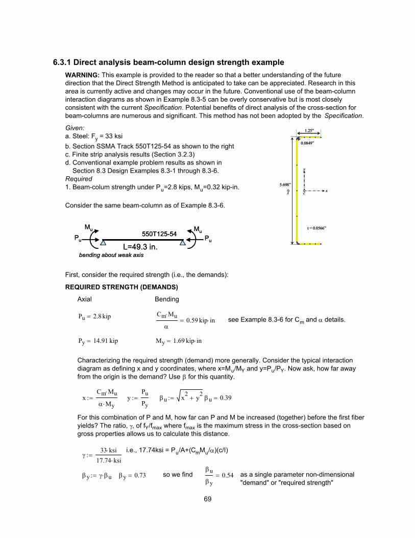
as a single parameter non-dimensional "demand" or "required strength"
βu
βy0.54=so we findβy 0.73=βy γ βu⋅:=
γ33 ksi⋅
17.74 ksi⋅:=
i.e., 17.74ksi = Pu/A+(CmMu/α)(c/I)
For this combination of P and M, how far can P and M be increased (together) before the first fiber yields? The ratio, γ, of fY/fmax where fmax is the maximum stress in the cross-section based on gross properties allows us to calculate this distance.
βu 0.39=βu x2 y2+:=y
Pu
Py:=x
Cm Mu⋅
α My⋅:=
Characterizing the required strength (demand) more generally. Consider the typical interaction diagram as defining x and y coordinates, where x=Mu/MY and y=Pu/PY. Now ask, how far away from the origin is the demand? Use β for this quantity.
My 1.69 kip in⋅=Py 14.91 kip=
see Example 8.3-6 for Cm and α details.Cm Mu⋅
α0.59 kip in⋅=
Pu 2.8 kip=
Bending Axial
REQUIRED STRENGTH (DEMANDS)
First, consider the required strength (i.e., the demands):
Pu
Mu
Pu
Mu
L=49.3 in.
550T125-54
bending about weak axis
Pu
Mu
Pu
Mu
L=49.3 in.
550T125-54
bending about weak axis
Consider the same beam-column as of Example 8.3-6.
Given: a. Steel: Fy = 33 ksib. Section SSMA Track 550T125-54 as shown to the rightc. Finite strip analysis results (Section 3.2.3)d. Conventional example problem results as shown in Section 8.3 Design Examples 8.3-1 through 8.3-6.Required1. Beam-colum strength under Pu=2.8 kips, Mu=0.32 kip-in. 5.698”
1.25”
0.0849”
t = 0.0566”
x
y
cs
5.698”
1.25”
0.0849”
t = 0.0566”
x
y
cs
WARNING: This example is provided to the reader so that a better understanding of the future direction that the Direct Strength Method is anticipated to take can be appreciated. Research in this area is currently active and changes may occur in the future. Conventional use of the beam-column interaction diagrams as shown in Example 8.3-5 can be overly conservative but is most closely consistent with the current Specification. Potential benefits of direct analysis of the cross-section for beam-columns are numerous and significant. This method has not been adopted by the Specification.
6.3.1 Direct analysis beam-column design strength example
69
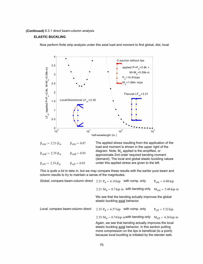
Again, we see that bending actually improves the local elastic buckling axial behavior, in this section putting more compression on the lips is beneficial (to a point) because local buckling is initiated by the slender web.
Mcrl 4.26 kip in⋅=with bending only 2.35 Mu⋅ 0.74 kip in⋅=
Pcrl 5.52 kip=with comp. only 2.35 Pu⋅ 6.57 kip=Local, compare beam-column direct
We see that the bending actually improves the global elastic buckling axial behavior.
Mcre 5.48 kip in⋅=with bending only 2.21 Mu⋅ 0.7 kip in⋅=
Pcre 6.08 kip=with comp. only 2.21 Pu⋅ 6.18 kip=Global, compare beam-column direct
This is quite a lot to take in, but we may compare these results with the earlier pure beam and column results to try to maintain a sense of the magnitudes.
βcrl 0.93=βcrl 2.35 βu⋅:=
βcrd 0.93=βcrd 2.35 βu⋅:=
The applied stress resulting from the application of the load and moment is shown in the upper right of the diagram. Note, Mu applied is the amplified, or approximate 2nd order required bending moment (demand). The local and global elastic buckling values under this applied stress are given to the left.
βcre 0.87=βcre 2.21 βu⋅:=
100 101 102 1030
0.5
1
1.5
2
2.5
3
3.5
4
half-wavelength (in.)
LFcr
(app
lied
P=P
u=2.8
k, M
=Mu=0
.59k
-in)
C-section without lips
applied P=Pu=2.8k +
M=Mu=0.59k-in
Py=14.91kips
My=1.69in.-kips
Local/Distortional LFcr=2.35
Flexural LFcr=2.21
Now perform finite strip analysis under this axial load and moment to find global, dist, local
ELASTIC BUCKLING
(Continued) 6.3.1 direct beam-column analysis
70
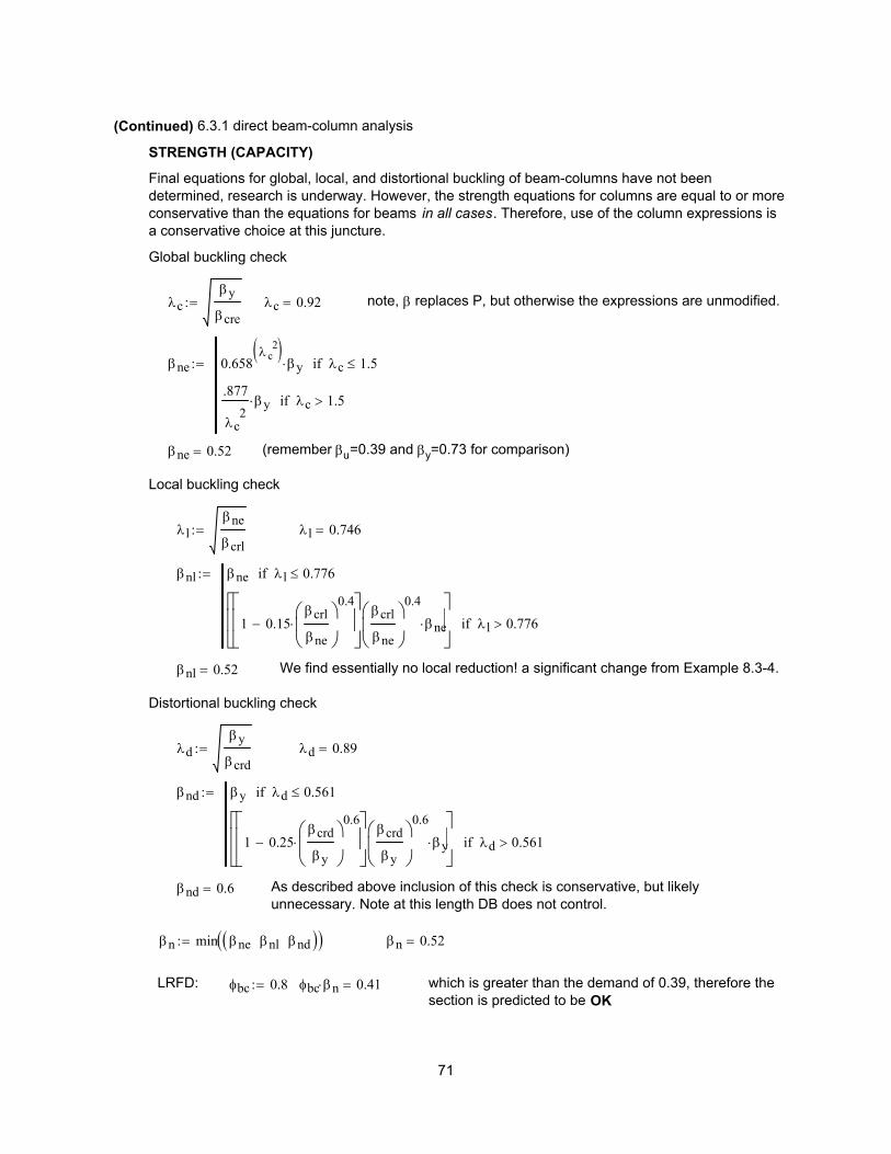
which is greater than the demand of 0.39, therefore the section is predicted to be OK
φbc βn⋅ 0.41=φbc 0.8:=LRFD:
βn 0.52=βn min βne βnl βnd( )( ):=
As described above inclusion of this check is conservative, but likely unnecessary. Note at this length DB does not control.
βnd 0.6=
βnd βy λd 0.561≤if
1 0.25βcrd
βy
0.6
⋅−
βcrd
βy
0.6
βy⋅
λd 0.561>if
:=
λd 0.89=λdβy
βcrd:=
Distortional buckling check
We find essentially no local reduction! a significant change from Example 8.3-4.βnl 0.52=
βnl βne λl 0.776≤if
1 0.15βcrl
βne
0.4
⋅−
βcrl
βne
0.4
βne⋅
λl 0.776>if
:=
λl 0.746=λlβne
βcrl:=
Local buckling check
(remember βu=0.39 and βy=0.73 for comparison)βne 0.52=
βne 0.658λ c
2( )βy⋅ λc 1.5≤if
.877
λc2βy⋅ λc 1.5>if
:=
note, β replaces P, but otherwise the expressions are unmodified. λc 0.92=λcβy
βcre:=
Global buckling check
Final equations for global, local, and distortional buckling of beam-columns have not been determined, research is underway. However, the strength equations for columns are equal to or more conservative than the equations for beams in all cases. Therefore, use of the column expressions is a conservative choice at this juncture.
STRENGTH (CAPACITY)
(Continued) 6.3.1 direct beam-column analysis
71
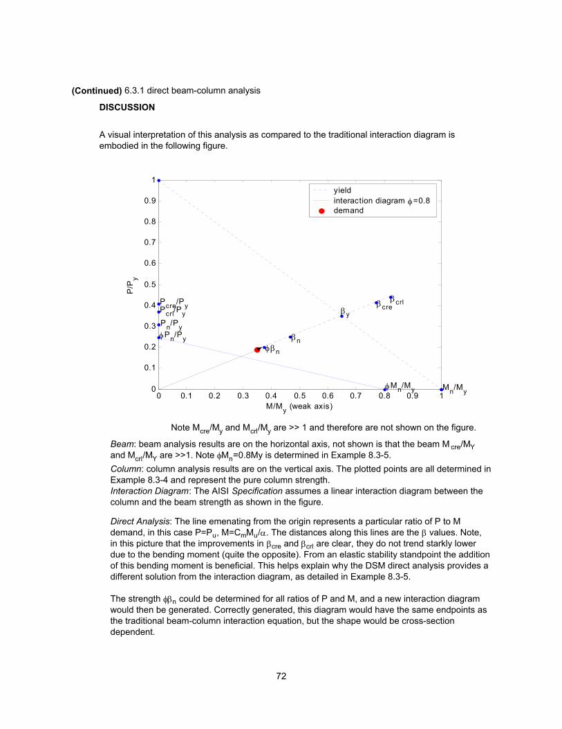
(Continued) 6.3.1 direct beam-column analysis
DISCUSSION
A visual interpretation of this analysis as compared to the traditional interaction diagram is embodied in the following figure.
0 0.1 0.2 0.3 0.4 0.5 0.6 0.7 0.8 0.9 10
0.1
0.2
0.3
0.4
0.5
0.6
0.7
0.8
0.9
1
Pcrl/Py
Pcre/Py
Pn/PyφPn/Py
Mn/MyφMn/My
βcrlβcreβy
βnφβn
M/My (weak axis)
P/P
y
y ieldinteraction diagram φ=0.8demand
Note Mcre/My and Mcrl/My are >> 1 and therefore are not shown on the figure.
Beam: beam analysis results are on the horizontal axis, not shown is that the beam M cre/MY and Mcrl/MY are >>1. Note φMn=0.8My is determined in Example 8.3-5.Column: column analysis results are on the vertical axis. The plotted points are all determined in Example 8.3-4 and represent the pure column strength.Interaction Diagram: The AISI Specification assumes a linear interaction diagram between the column and the beam strength as shown in the figure.
Direct Analysis: The line emenating from the origin represents a particular ratio of P to M demand, in this case P=Pu, M=CmMu/α. The distances along this lines are the β values. Note, in this picture that the improvements in βcre and βcrl are clear, they do not trend starkly lower due to the bending moment (quite the opposite). From an elastic stability standpoint the addition of this bending moment is beneficial. This helps explain why the DSM direct analysis provides a different solution from the interaction diagram, as detailed in Example 8.3-5.
The strength φβn could be determined for all ratios of P and M, and a new interaction diagram would then be generated. Correctly generated, this diagram would have the same endpoints as the traditional beam-column interaction equation, but the shape would be cross-section dependent.
72
73
7 Product development
7.1 Cross-section optimization The examples of Chapter 3 and 8 provide some preliminary ideas on the optimization of cold-formed steel cross-sections. The given ideas are preliminary, and are not intended to suggest globally improved cross-sections. Nor are formal methods used for creating these improved cross-sections. The Direct Strength Method provides a tool that allows improvements in the cross-section to be examined by analysis, without testing, and without the inherent limitations of the existing provisions which focus on a limited number of cross-section types. In most situations, the addition of small longitudinal stiffeners can greatly enhance the local buckling strength of cold-formed steel cross-sections. However, distortional buckling and global buckling are largely unaffected by such small changes. Thus, more creative enhancements may be pursued to increase distortional and/or global bucking strength. Optimal designs predicted by the Direct Strength Method are known to be different from those predicted by simply manipulating the main Specification equations. One specific example of this: edge stiffeners are encouraged to be longer in DSM than in the main Specification. Optimal designs also depend on the resistance (or safety) factor. Since, pre-qualified geometries employ higher φ factors (and lower Ω factors) than other geometries, which must follow rational analysis. Sections 7.3 and 7.4 of this Guide discuss this in greater detail and provide some basic advice on how to begin the process of determining the appropriate φ or Ω factor for cross-sections that are not pre-qualified. Final optimization will have as much, if not more to do with manufacturing, constructability, and other practical matters; however, DSM provides a way to quantitatively focus on the strength improvements available to cold-formed steel designers/manufacturers. Cold-formed steel is a versatile, easily formed material – it is one objective of this Guide to help manufacturers take better advantage of the potential in cold-formed steel for creating optimal cross-section shapes.
7.2 Developing span and load tables The solutions for beam charts and column charts discussed in Chapters 4 and 5 respectively, and demonstrated in Examples 8.13 and 8.14 respectively, provide the basis for developing span and load tables as typically generated by manufacturers. Automation of the process of developing span and load tables is only possible once the elastic buckling values have been determined. Generally, determination of Pcrl, Pcrd, Pcre and/or Mcrl, Mcrd, and Mcre requires some manual interaction with an FSM program, etc. Once these values are established, and following the examples (8.13 and 8.14), their variation with unbraced length established, then developing the necessary tables is straightforward. Special care must be taken with resistance or safety factors (φ or Ω) since the DSM values may be different from the main Specification.

74
7.3 Rational analysis vs. chapter F testing For a developed cross-section not covered by the main Specification provisions two basic avenues exist for strength prediction, as outlined in main Specification A1.1(b):
(a) determine the strength by testing and find φ via Chapter F of the Specification, or (b) determine the strength by rational analysis and use the blanket φ provided.
The resistance factor (φ) for these two basic choices are shown in Figure 40.
Members USA and Mexico Canada
Ω (ASD) φ (LRFD) φ (LSD) 2.00 0.80 0.75
( )2Q
2PP
2F
2Mo VVCVV
mmm ePFMC +++β−φ=φ
(a) rational analysis resistance factor (b) resistance factor based on Chapter F Figure 40 Resistance factor determination for a new cross-section
The rational analysis φ factor of 0.8 is lower (more conservative) than the typical φ factors for beams (0.9 to 0.95) and columns (0.85). However, when compared with a method relying solely on testing (Chaper F), there is an incentive towards rational analysis methods. If rational analysis is not employed, and instead the strength prediction of a member is based solely on testing, then the provisions of Chapter F of the main Specification apply. In particular, the expression of Figure 40(b) governs. The number of tests required to generate a more favorable resistance factor than the rational analysis procedure can be considerable, and depends on the scatter (coefficient of variation) of the test results. Given the rational analysis φ value of 0.8, Figure 41 shows that for typical test scatter (VP=15%) at least 11 tests must be performed before a pure test method generates a φ > 0.80. If the scatter is less, fewer tests are needed. To generate φ factors as high as the pre-qualified Direct Strength Method expressions the scatter must be low and a significant number of tests must be performed. Given that testing is generally costly, and scatter is inherent in cold-formed steel systems (a low VP is hard to achieve) the rational analysis method φ (resistance) factor is a definite incentive.
5 10 15 20 25 300.7
0.75
0.8
0.85
0.9
φ
number of tests (n)
rational analysis φ value
VP=6.5% (minimum value)
VP=10% (low scatter)
VP=15% (typical scatter)
5 10 15 20 25 300.7
0.75
0.8
0.85
0.9
φ
number of tests (n)
rational analysis φ value
VP=6.5% (minimum value)
VP=10% (low scatter)
VP=15% (typical scatter)
Figure 41 Relationship between number of tests and φ for
Chapter F method

75
7.4 New pre-qualified members and extending the bounds of a pre-qualified member
No formal method yet exists in the Specification for extending the Direct Strength Method to additional (new) pre-qualifed members, or extending the bounds for existing pre-qualified members. Currently, to extend the bounds or add an additional cross-section, a formal ballot vote of the AISI Committee on Specifications is required. As shown in the example problems of Chapter 8 the pre-qualified φ factors make a significant difference in determining the design strength, and hence optimum member design. If logical, it would be desirable for new cross-sections or cross-sections that slightly violate existing pre-qualified bounds to employ the pre-qualified resistance factors. To justify such use it must be ensured that the reliability of the design strength is not compromised. This requires one to take a closer look at how the reliability of the Direct Strength Method was determined. Table 5 is provided to help the user of this Guide to better understand the statistics underlying the reliability of the Direct Strength Method. This table shows the number of samples (n), the mean test-to-predicted ratio for DSM (Pm) and the coefficient of variation of the test-to-predicted ratio (VP) for each of the cross-section types identified in Tables 1.1.1-1 and 1.1.1-2 in DSM. These statistics, in conjunction with the method outlined in Chapter F, provide the evidence that the pre-qualified members can meet (or exceed) the target reliability, and thus may use higher φ factors than the Section A1.1(b) rational analysis values. Thus φ for pre-qualified beams is 0.9 and φ for pre-qualified columns is 0.85.
Table 5 Summary Statistics for DSM Development n Pm VP
BeamsC-sections 185 1.10 0.11C-sections with web stiffeners 42 1.12 0.07Z-sections 48 1.13 0.13Hat sections 186 1.10 0.15Trapezoidal sections 98 1.01 0.13
ALL BEAMS 559 1.09 0.12ColumnsC-sections 114 1.01 0.15C-sections with web stiffeners1 29 0.88 0.14Z-sections 85 0.96 0.13Rack sections 17 1.02 0.05Hat sections 4 0.98 0.02
ALL COLUMNS 249 0.98 0.14 (1) Thomasson's (1978) tests contribute to the low Pm, more recent tests by Kwon and Hancock (1992) showed much better agreement.
New cross-section: consider the case where one is interested in pre-qualifying an entirely new cross-section. Do three or more tests. Generate a φ using Chapter F, but use the test-to-predicted ratio with DSM as the prediction to generate the professional factor Pm, and use the coefficient of variation of the test-to-predicted ratio for VP. (In a method relying solely on testing PM is 1.0 and VP is the scatter in the test results, here Pm is the mean accuracy of the predicting method, and VP

76
is the scatter in the predicting method). If the φ produced is greater than or equal to a DSM pre-qualified cross-section (φ=0.9 for beams, φ=0.85 for columns) this is strong evidence that the cross-section should be pre-qualified. The proposed bounds for the new cross-section would be the bounds of the testing. Pilot tests for a new cross-section: consider the case where pilot tests on a new cross-section are being considered but a large battery of tests cannot be performed at the time. Assuming only a small number of tests can be performed the following procedure is suggested. Perform at least three tests and determine the average test-to-predicted ratio for DSM (Pm
*). For the coefficient of variation for the method (VP) assume the worst VP observed in Table 5, 15%. Set the correction for sample size, Cp to 1.0. Estimating the mean with a small number of tests is more reliable than estimating VP, so this method attempts to assure that the reliability (in essence, φ) is met, by assuming that the variation (VP) is the most conservative VP observed to date. Now, determine the resistance factor φ, via Chapter F of the main Specification. If the φ produced is greater than or equal to a DSM pre-qualified cross-section (φ=0.9 for beams, φ=0.85 for columns) this is evidence that the cross-section should be pre-qualified. A lower φ is not cause for immediate rejection, but does suggest more tests or a revised strength prediction equation may be needed. Extend the bounds: consider the case where engineering judgment makes it clear that a cross-section fits in one of the pre-qualified categories, but one or more of the geometric bounds are violated. If a large battery of tests can be performed then the procedure could follow that of a new cross-section as described in the preceding paragraphs. Assuming only a small number of tests can be performed the following procedure is suggested. Perform at least three tests and determine the average test-to-predicted ratio for DSM (Pm
*). If the Pm* of the three tests is equal
to or greater than the comparable pre-qualified category (Table 5), then the bounds should likely be extended. Estimating the mean with a small number of tests is more reliable than estimating VP, so this method assures that the reliability (in essence, φ) is met, by assuming that the variation (VP) in the newly tested cross-sections is equal to that of the underlying category. In no way does a lower Pm
* preclude that the cross-section should be pre-qualified, but additional testing will likely be required. Notes: The preceding procedures do not guarantee the cross-section will be pre-qualified; they are an attempt to provide manufacturers with the best current advice. Currently, testing and calculation evidence would need to be taken to the AISI Committee on Specifications in the form of a ballot for consideration to extend pre-qualified cross-sections. All test results would need to be available to the public. All quantities should be measured, not nominal. The thickness should be the measured base metal thickness, the yield stress should be based on tensile coupons from the as-formed cross-section, and the dimensions should be based on direct measurement. For ASD Ω can be calculated from φ via main Specification Equation F1.2-2.
77
8 Design examples
The Design Example presented here include those cross-sections employed in the AISI (2002) Design Manual plus additional cross-sections selected to highlight the use of the Direct Strength Method for more complicated and optimized members. The following cross-sections are considered:
8.1 C-section with lips, 8.2 C-section with lips modified, 8.3 C-section without lips (track section), 8.4 C-section without lips (track section) modified, 8.5 Z-section with lips, 8.6 Z-section with lips modified, 8.7 Equal leg angle with lips, 8.8 Equal leg angle, 8.9 Hat section, 8.10 Wall panel section, 8.11 Rack post section, and a 8.12 Sigma section.
The relationship between the AISI (2002) Design Manual examples and the Design Examples of this Guide are provided for beams in Table 2 of Section 4.5, for columns in Table 3 of Section 5.3, and for beam-columns in Table 4 of Section 6.2. Numerical comparison of the predicted strength between DSM and the main Specification is provided in Section 8.15 of this Guide. For each cross-section the design flexural strength for a fully braced beam and the design compressive strength for a continuously braced column are provided. For most cross-sections additional design strength values for discrete bracing in bending and compression are provided. For the C-section with lips, C-section without lips, Equal leg angle, and the hat section, beam-column examples are provided. The Design Examples were prepared using Mathcad. For readers unfamiliar with the notations used in this software please see the Quick Start guide on page ii of this Guide. Also, to better understand how Mathcad works and to enable the reader to check intermediate calculation values Design Example 8.1.1 is completed in standard Mathcad format and in an extended format. In the extended format all values are explicitly substituted into the equations and all intermediate calculation results are provided to the reader. The Design Examples given in Sections 8.13 and 8.14 provide the complete solution for developing beam charts and column charts, respectively. The cross-sections employed in these examples are the C-section with lips and the C-section with lips modified.
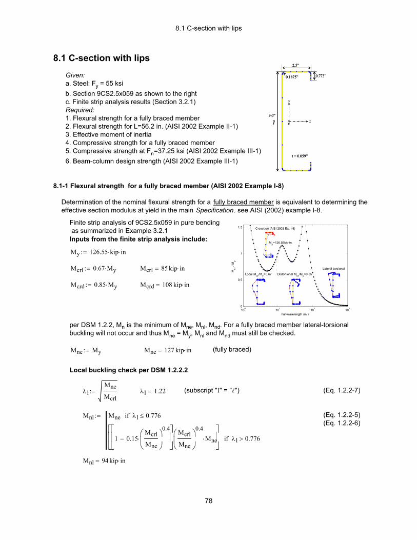
8.1 C-section with lips
Mnl 94 kip in⋅=
(Eq. 1.2.2-5)(Eq. 1.2.2-6)
Mnl Mne λl 0.776≤if
1 0.15Mcrl
Mne
0.4
⋅−
Mcrl
Mne
0.4
Mne⋅
λl 0.776>if
:=
(Eq. 1.2.2-7)(subscript "l" = "l")λl 1.22=λlMne
Mcrl:=
Local buckling check per DSM 1.2.2.2
(fully braced)Mne 127 kip in⋅=Mne My:=
per DSM 1.2.2, Mn is the minimum of Mne, Mnl, Mnd. For a fully braced member lateral-torsional buckling will not occur and thus Mne = My, Mnl and Mnd must still be checked.
Mcrd 108 kip in⋅=Mcrd 0.85 My⋅:=
Mcrl 85 kip in⋅=Mcrl 0.67 My⋅:=
My 126.55 kip⋅ in⋅:=
Inputs from the finite strip analysis include:
Finite strip analysis of 9CS2.5x059 in pure bending as summarized in Example 3.2.1
100 101 102 1030
0.5
1
1.5
half-wavelength (in.)
Mcr
/ M
y C-section (AISI 2002 Ex. I-8)
My=126.55kip-in.
Local Mcr/My=0.67 Distortional Mcr/My=0.85
Lateral-torsional
Determination of the nominal flexural strength for a fully braced member is equivalent to determining the effective section modulus at yield in the main Specification. see AISI (2002) example I-8.
8.1-1 Flexural strength for a fully braced member (AISI 2002 Example I-8)
Given: a. Steel: Fy = 55 ksib. Section 9CS2.5x059 as shown to the rightc. Finite strip analysis results (Section 3.2.1)Required:1. Flexural strength for a fully braced member2. Flexural strength for L=56.2 in. (AISI 2002 Example II-1)3. Effective moment of inertia4. Compressive strength for a fully braced member5. Compressive strength at Fn=37.25 ksi (AISI 2002 Example III-1)6. Beam-column design strength (AISI 2002 Example III-1)
9.0”
2.5”
0.773”0.1875”
t = 0.059”
x
y
cs
9.0”
2.5”
0.773”0.1875”
t = 0.059”
x
y
cs
8.1 C-section with lips
78
8.1 C-section with lips
The calibration of R factors was performed to the main Specification. The main Specification does not include an explicit check for distortional buckling. Therefore, if distortional buckling (M nd) controls the strength the uplift prediction using R may be excessively conservative. Here M nd~Mnl and it is expected that the prediction is reasonably accurate.
nominal flexural strength in upliftR Mn⋅ 55.81 kip in⋅=R 0.6:=uplift:
Part 4 of the AISI (2002) Design Manual Example II-1 calculates the nominal flexural strength in uplift of this cross-section. The formula is RSeFY, where SeFY is the fully braced flexural strength and R is an empirical factor from main Specificiation C3.1.3. If the conditions of C3.1.3 are met, flexural strength in uplift can be found using this simple manner. For this example R=0.6
Note on uplift
Mn
Ωb56 kip in⋅=Ωb 1.67:=ASD:
φb Mn⋅ 84 kip in⋅=φb 0.9:=LRFD:
The geometry of this section falls within the "pre-qualified" beams of DSM 1.1.1.2 and the higher φ and lower Ω of DSM Section 1.2.2 may therefore be used.
Mn 93 kip in⋅=Mn min Mne Mnl Mnd( )( ):=
Predicted flexural strength per DSM 1.3
Mnd 93 kip in⋅=
(Eq. 1.2.2-8)(Eq. 1.2.2-9)
Mnd My λd 0.673≤if
1 0.22Mcrd
My
0.5
⋅−
Mcrd
My
0.5
My⋅
λd 0.673>if
:=
(Eq. 1.2.2-10)λd 1.08=λdMy
Mcrd:=
Distortional buckling check per DSM 1.2.2.3
(Continued) 8.1-1 Flexural strength for a fully braced member
79
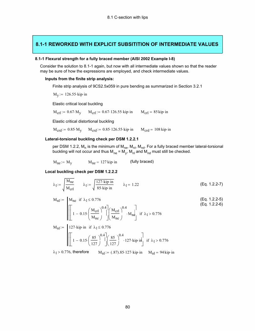
8.1 C-section with lips
Mnl 94 kip in⋅=Mnl .87( ).85 127⋅ kip⋅ in⋅:=λl 0.776> , therefore
Mnl 127 kip⋅ in⋅ λl 0.776≤if
1 0.1585127
0.4⋅−
85127
0.4127⋅ kip⋅ in⋅
λl 0.776>if
:=
(Eq. 1.2.2-5)(Eq. 1.2.2-6)
Mnl Mne λl 0.776≤if
1 0.15Mcrl
Mne
0.4
⋅−
Mcrl
Mne
0.4
Mne⋅
λl 0.776>if
:=
(Eq. 1.2.2-7)λl 1.22=λl127 kip⋅ in⋅85 kip⋅ in⋅
:=λlMne
Mcrl:=
Local buckling check per DSM 1.2.2.2
(fully braced)Mne 127 kip in⋅=Mne My:=
per DSM 1.2.2, Mn is the minimum of Mne, Mnl, Mnd. For a fully braced member lateral-torsional buckling will not occur and thus Mne = My, Mnl and Mnd must still be checked.
Lateral-torsional buckling check per DSM 1.2.2.1
Mcrd 108 kip in⋅=Mcrd 0.85 126.55⋅ kip⋅ in⋅:=Mcrd 0.85 My⋅:=
Elastic critical distortional buckling
Mcrl 85 kip in⋅=Mcrl 0.67 126.55⋅ kip⋅ in⋅:=Mcrl 0.67 My⋅:=
Elastic critical local buckling
My 126.55 kip⋅ in⋅:=
Finite strip analysis of 9CS2.5x059 in pure bending as summarized in Section 3.2.1
Inputs from the finite strip analysis:
Consider the solution to 8.1-1 again, but now with all intermediate values shown so that the reader may be sure of how the expressions are employed, and check intermediate values.
8.1-1 Flexural strength for a fully braced member (AISI 2002 Example I-8)
8.1-1 REWORKED WITH EXPLICIT SUBSITITION OF INTERMEDIATE VALUES
80
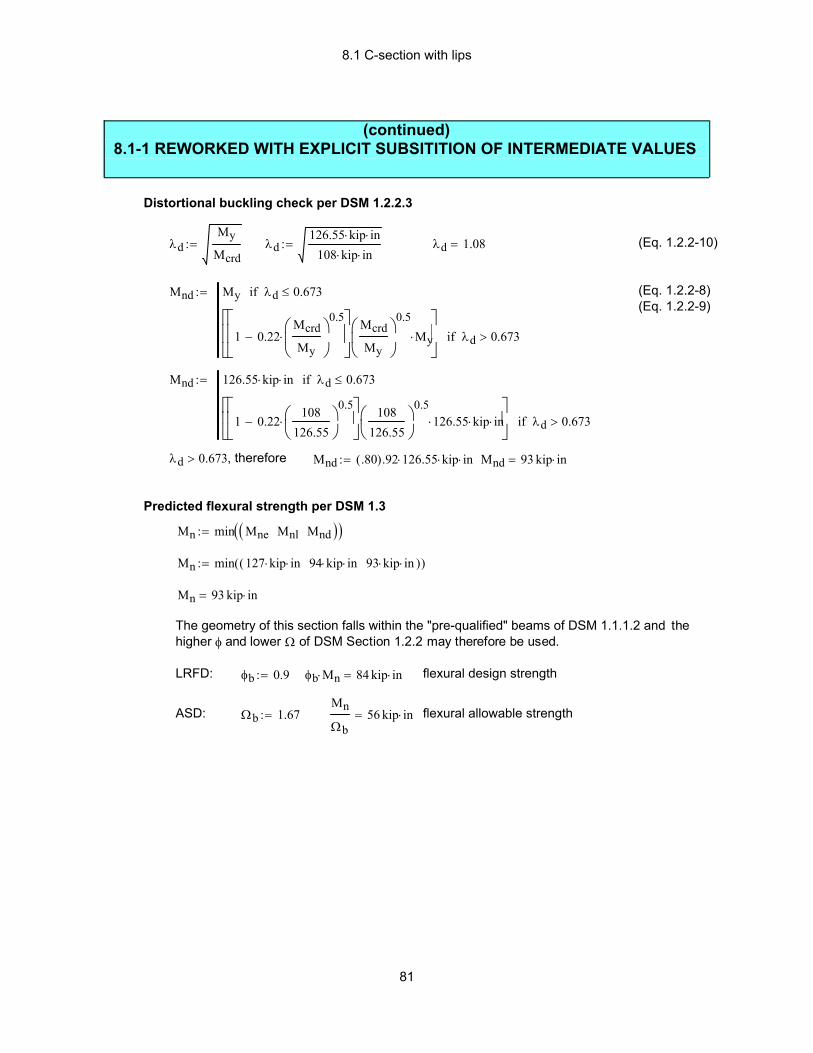
8.1 C-section with lips
flexural allowable strengthMn
Ωb56 kip in⋅=Ωb 1.67:=ASD:
flexural design strengthφb Mn⋅ 84 kip in⋅=φb 0.9:=LRFD:
The geometry of this section falls within the "pre-qualified" beams of DSM 1.1.1.2 and the higher φ and lower Ω of DSM Section 1.2.2 may therefore be used.
Mn 93 kip in⋅=
Mn min 127 kip⋅ in⋅ 94 kip⋅ in⋅ 93 kip⋅ in⋅( )( ):=
Mn min Mne Mnl Mnd( )( ):=
Predicted flexural strength per DSM 1.3
Mnd 93 kip in⋅=Mnd .80( ).92 126.55⋅ kip⋅ in⋅:=λd 0.673> , therefore
Mnd 126.55 kip⋅ in⋅ λd 0.673≤if
1 0.22108
126.55
0.5⋅−
108126.55
0.5126.55⋅ kip⋅ in⋅
λd 0.673>if
:=
(Eq. 1.2.2-8)(Eq. 1.2.2-9)
Mnd My λd 0.673≤if
1 0.22Mcrd
My
0.5
⋅−
Mcrd
My
0.5
My⋅
λd 0.673>if
:=
(Eq. 1.2.2-10)λd 1.08=λd126.55 kip⋅ in⋅
108 kip⋅ in⋅:=λd
My
Mcrd:=
Distortional buckling check per DSM 1.2.2.3
(continued)8.1-1 REWORKED WITH EXPLICIT SUBSITITION OF INTERMEDIATE VALUES
81
8.1 C-section with lips
Mne 126.55 kip in⋅=
Local buckling check per DSM 1.2.2.2
unchanged from Example 8.1-1 Mnl 94 kip in⋅=
Distortional buckling check per DSM 1.2.2.3
unchanged from Example 8.1-1 Mnd 93 kip in⋅=
Predicted flexural strength per DSM 1.3
Mn min Mne Mnl Mnd( )( ):= Mn 93 kip in⋅=
The geometry of this section falls within the "pre-qualified" beams of DSM Section 1.1.1.2 and the higher φ and lower Ω of DSM Section 1.2.2 may therefore be used.
LRFD: φb 0.9:= φb Mn⋅ 84 kip in⋅= Note, that φb from DSM Section 1.2.2 is 0.90, not 0.95 as in the main Specification.
ASD: Ωb 1.67:=Mn
Ωb56 kip in⋅=
Further notes on AISI (2002) Design Example II-1: Design checks for shear could follow the nomenclature of Section 4.4.1 of this Guide. Design checks for web crippling are unmodified from theAISI (2002) example. In the design checks for combined bending and shear, and combined bending and crippling φMnxo could be replaced by the results for φMn from Example 8.1-1.
8.1-2 Flexural strength for L=56.2 in. (AISI 2002 Example II-1)
AISI (2002) Example II-1 provides a complete calculation for a 4 span continuous beam. The following calculation provides an alternative means to calculate the flexural design strength of one of the spans. Namely, an interior span where Ly=Lt=56.2 in., and Cb = 1.67 (conservatively assumed as a linear moment diagram between the inflection point and support).
Inputs from the finite strip analysis include:
Local and distortional are unchanged from Example 8.1-1
Global (lateral-torsional) buckling may be found directly from the finite strip analysis plot
Mcre 1.73 My⋅:= for Cb=1 at Ly=Lt=56.2 in. Mcre 218.93 kip in⋅=
Lateral-torsional buckling check per DSM 1.2.2.1
per AISI (2002) Example II-1 Cb 1.67:=
Mcre Cb Mcre⋅:=Mcre
My2.89= per upperbounds of Section 2.2 Mne=My!
more formally,
Mne Mcre Mcre 0.56 My⋅<if
109
My⋅ 110 My⋅
36 Mcre⋅−
⋅
2.78 My⋅ Mcre≥ 0.56 My⋅≥if
My Mcre 2.78 My⋅>if
:= (Eq. 1.2.2-1)
(Eq. 1.2.2-2)
(Eq. 1.2.2-3)
82
8.1 C-section with lips
Mdl Mde λl 0.776≤if
1 0.15Mcrl
Mde
0.4
⋅−
Mcrl
Mde
0.4
Mde⋅
λl 0.776>if
:= (Eq. 1.2.2-5)(Eq. 1.2.2-6)
Mdl 54.3 kip in⋅=
Determine Mdd for distortional buckling (per DSM 1.2.2.3)
replace My with M as stated in Eq. 1.1.3-1
λdM
Mcrd:= λd 0.72= Note My replaced with M (Eq. 1.2.2-10)
Mdd M λd 0.673≤if
1 0.22Mcrd
M
0.5
⋅−
Mcrd
M
0.5
M⋅
λd 0.673>if
:= (Eq. 1.2.2-8)(Eq. 1.2.2-9)
Mdd 53.9 kip in⋅=
Final Md for determining the reduced moment of inertia in Eq. 1.1.3-1
Md min Mde Mdd Mdl( )( ):= Md 53.9 kip in⋅=
IeffMd
MIg⋅:= < Ig (Eq. 1.1.3-1)
Ieff 9.93 in4=
Ieff
Ig0.96= At a demand of 60% of the nominal moment capacity the
predicted stiffness is 96% of the gross moment of inertia.
8.1-3 Effective Moment of Inertia (AISI 2002 Example I-8)
The Direct Strength Method prescribes that the reduction in the bending stiffness can be determined by finding the ratio of the nominal flexural strength at service loads (Md) to the applied loads, M.
IeffMd
MIg⋅:=
M< Ig (Eq. 1.1.3-1)
M: Consider a service load at 60% of nominal strength (where Mn = 93 kip-in. from Example 8.1-1)
M 0.6 Mn⋅:= M 55.88 kip in⋅=
Md: local/distortional strength reduction at required (demand) M
Mcrl and Mcrd from finite strip analysis remain the same as given in Examples 8.1-1 and 8.1-2
Determine Mde for global buckling (per DSM 1.2.2.1) (replace My with M as stated in Eq. 1.1.3-1)
For a fully braced section, or for the scenario of Example 8.1-2, M cre>2.78M therefore, per Eq. 1.2.2-3 no reduction will occur due to global buckling.
Mde M:= (Eq. 1.2.2-3)
Mde 55.88 kip in⋅= note subscript "n" is replaced with "d" to denote deflection calculation, so Mne becomes Mde, Mnl becomes Mdl and Mnd becomes Mdd....
Determine Mdl for local buckling (per DSM 1.2.2.2)
λlMde
Mcrl:= λl 0.81= Note Mne replaced with Mde (Eq. 1.2.2-7)
83
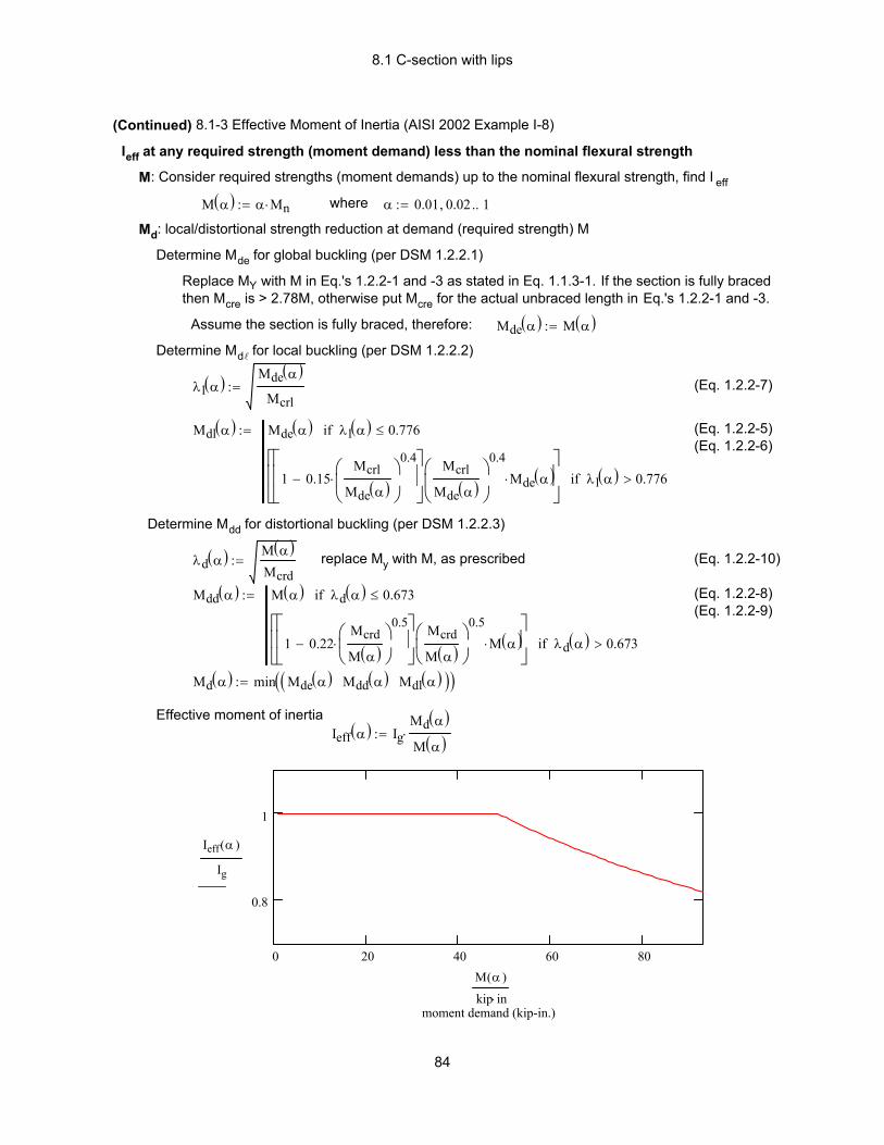
8.1 C-section with lips
0 20 40 60 80
0.8
1
moment demand (kip-in.)
Ieff α( )
Ig
M α( )
kip in⋅
Ieff α( ) IgMd α( )M α( )⋅:=
Effective moment of inertia
Md α( ) min Mde α( ) Mdd α( ) Mdl α( )( )( ):=
(Eq. 1.2.2-8)(Eq. 1.2.2-9)
Mdd α( ) M α( ) λd α( ) 0.673≤if
1 0.22Mcrd
M α( )
0.5
⋅−
Mcrd
M α( )
0.5
M α( )⋅
λd α( ) 0.673>if
:=
(Eq. 1.2.2-10)replace My with M, as prescribedλd α( ) M α( )Mcrd
:=
Determine Mdd for distortional buckling (per DSM 1.2.2.3)
(Eq. 1.2.2-5)(Eq. 1.2.2-6)
Mdl α( ) Mde α( ) λl α( ) 0.776≤if
1 0.15Mcrl
Mde α( )
0.4
⋅−
Mcrl
Mde α( )
0.4
Mde α( )⋅
λl α( ) 0.776>if
:=
(Eq. 1.2.2-7)λl α( ) Mde α( )Mcrl
:=
Determine Mdl for local buckling (per DSM 1.2.2.2)
Mde α( ) M α( ):=Assume the section is fully braced, therefore:
Replace MY with M in Eq.'s 1.2.2-1 and -3 as stated in Eq. 1.1.3-1. If the section is fully braced then Mcre is > 2.78M, otherwise put Mcre for the actual unbraced length in Eq.'s 1.2.2-1 and -3.
Determine Mde for global buckling (per DSM 1.2.2.1)
Md: local/distortional strength reduction at demand (required strength) M
α 0.01 0.02, 1..:=where M α( ) α Mn⋅:=
M: Consider required strengths (moment demands) up to the nominal flexural strength, find I eff
Ieff at any required strength (moment demand) less than the nominal flexural strength
(Continued) 8.1-3 Effective Moment of Inertia (AISI 2002 Example I-8)
84

8.1 C-section with lips
Pnl 19.4 kip= (note the significant post-buckling strength, P crl is only 5.8 kips)
Distortional buckling check per DSM 1.2.1.3
λdPy
Pcrd:= λd 1.92= (Eq. 1.2.1-10)
Pnd Py λd 0.561≤if
1 0.25Pcrd
Py
0.6
⋅−
Pcrd
Py
0.6
Py⋅
λd 0.561>if
:= (Eq. 1.2.1-8)(Eq. 1.2.1-9)
Pnd 19.6 kip=
Predicted compressive capacity per DSM 1.2
Pn min Pne Pnl Pnd( )( ):= Pn 19.4 kip=
The geometry of this section falls within the "pre-qualified" columns of DSM Section 1.1.1.1 and the higher φ and lower Ω of DSM Section 1.2.1 may therefore be used.
LRFD: φc 0.85:= φc Pn⋅ 16.5 kip= ASD: Ωc 1.80:=Pn
Ωc10.8 kip=
8.1-4 Compressive strength for a continuously braced column (AISI 2002 Example I-8)
Finite strip analysis of 9CS2.5x059 in pure compression is summarized in Example 3.2.1
100 101 102 1030
0.05
0.1
0.15
0.2
0.25
0.3
0.35
0.4
half-wavelength (in.)
Pcr
/ P
y
C-section (AISI 2002 Ex. I-8)
Py=48.42kips
Local Pcr/Py=0.12
Distortional Pcr/Py=0.27
Flexural
Inputs from the finite strip analysis include:
Py 48.42 kip⋅:=
Pcrl 0.12 Py⋅:= Pcrl 5.8 kip=
Pcrd 0.27 Py⋅:= Pcrd 13.1 kip=
per DSM 1.2.1, Pn is the minimum of Pne, Pnl, Pnd. If a column is continuously braced then global buckling Pne is restricted and the squash load will develop if the section is compact.Pne Py:= Pne 48.42 kip=
Local buckling check per DSM 1.2.1.2
λlPne
Pcrl:= λl 2.89= (subscript "l" = "l") (Eq. 1.2.1-7)
Pnl Pne λl 0.776≤if
1 0.15Pcrl
Pne
0.4
⋅−
Pcrl
Pne
0.4
Pne⋅
λl 0.776>if
:= (Eq. 1.2.1-5)(Eq. 1.2.1-6)
85

8.1 C-section with lips
(reduced from 19.4 kips for a column with continuous bracing)Pnl 15.2 kip=
(Eq. 1.2.1-5)(Eq. 1.2.1-6)
Pnl Pne λl 0.776≤if
1 0.15Pcrl
Pne
0.4
⋅−
Pcrl
Pne
0.4
Pne⋅
λl 0.776>if
:=
(Eq. 1.2.1-7)λl 2.38=λlPne
Pcrl:=
(compare with λl of 2.9 for the same column with continuous bracing, see Example 8.1-4)
(from Example 8.1-4)Pcrl 5.8 kip=
Local buckling check per DSM 1.2.1.2
As demonstrated in AISI (2002) Example I-8, in the main Specification effective area (Ae) calculations for columns are performed at the stress that the long column can maintain, this stress known as Fn is calculated per Eq. C4-2 or C4-3. A similar procedure is perfomed in the Direct Strength Method where the local buckling slenderness and strength equations (DSM Eq.'s 1.2.1-7, and 1.2.1-5,6) are calculated at the strength a long column can maintain, i.e., P ne=AgFn
which is Fn of the main Specification.Pne
Ag37.26 ksi=The stress associated with this load is
Pne 32.8 kip=
(Eq. 1.2.1-3)
(Eq. 1.2.1-2)Pne 0.658λ c
2
Py⋅ λc 1.5≤if
.877
λc2
Py⋅ λc 1.5>if
:=
(Eq. 1.2.1-1)(inelastic regime)λc 0.96=λcPy
Pcre:=
Pcre 52.05 kip=Pcre Ag Fe⋅:=
(AISI 2002 Example III-1)Fe 59.12 ksi⋅:=
The strong axis elastic buckling stress may be found as detailed in AISI (2002) Example III-1, but involves nothing more than calculating Fe=π2E/(KLx/rx)2, for this section
The section is restricted so that it can only buckle about the strong axis. This restriction could be imposed on the finite strip model, as described in Section 3.4.6. However, this is more cumbersome than simply calculating the elastic buckling strength using closed-form formulas.
Flexural, Torsional, or Torsional-Flexural check per DSM 1.2.1.1
In AISI (2002) Example III-1 this 9CS2.5x059 is examined as a 20 ft. long beam-column. The section is simply-supported at its ends, and fully braced against lateral and torsional buckling. The compressive design strength of that beam-column is the subject of this example.
8.1-5 Compressive strength at Fn=37.25 ksi (AISI 2002 Example III-1)
86
8.1 C-section with lips
compressive allowable strengthPn
Ωc8.4 kip=Ωc 1.80:=ASD:
compressive design strengthφc Pn⋅ 12.91 kip=φc 0.85:=LRFD:
The geometry of this section falls within the "pre-qualified" columns of DSM Section 1.1.1.1 and the higher φ and lower Ω of DSM Section 1.2.1 may therefore be used.
Pn 15.2 kip=Pn min Pne Pnl Pnd( )( ):=
Predicted compressive strength per DSM 1.2
(note, the distortional buckling prediction is the same as Example 8.1-2)Pnd 19.6 kip=
(Eq. 1.2.1-8)(Eq. 1.2.1-9)
Pnd Py λd 0.561≤if
1 0.25Pcrd
Py
0.6
⋅−
Pcrd
Py
0.6
Py⋅
λd 0.561>if
:=
(Eq. 1.2.1-10)λd 1.92=λdPy
Pcrd:=
(from Example 8.1-4)Pcrd 13.1 kip=
Distortional buckling check per DSM 1.2.1.3
(Continued) 8.1-5 Compressive strength at Fn=37.25 ksi (AISI 2002 Example III-1)
87
8.1 C-section with lips
PEx 52.1 kip⋅:= from C5.2.1-6 as used in AISI (2002) Example III-1
PEx 53.7 kip⋅:= based on FSM analysis at 240 in., with x movement restricted. This PEx is used in this solution.
αx 0.93=
note, 2nd order required moment (demand) is approx.: Cmx Mux⋅
αx59.4 kip in⋅=
Interaction equationsPu
φc Pn⋅0.29= which is > 0.15, therefore use Equations C5.2.2-1 and C5.2.2-2
Pu
φc Pn⋅
Cmx Mux⋅
φb Mnx⋅ αx⋅+ 1= OK, but essentially at maximum value. (Eq. C5.2.2-1)
Pu
φc Pno⋅
Mux
φb Mnx⋅+ 0.89= OK. (Eq. C5.2.2-2)
for format of ASD solution see AISI (2002) Example III-1
8.1-6 Beam-column design (AISI 2002 Example III-1)
AISI (2002) design Example III-1 examines the strength of this 9CS2.25x059 as a beam-column. Consider the same beam-column as calculated via the Direct Strength Method here following the main Specification methodology.
Compression: the compressive strength of this section as determined in Example 8.1-5 above.
φc 0.85= Pn 15.18 kip=
for the interaction equation the fully braced compression strength is needed, per Example 8.1-4:
Pno 19.4 kip=
Bending: as discussed in Example 8.1-5 the section is fully braced against lateral and torsional movement, so the flexural strength is that of Example 8.1-1 above
φb 0.9= Mnx 93 kip in⋅=
Factors to account for approximate 2nd order analysis
Mux 55.2 kip⋅ in⋅:= First order required strength (moment demand) from AISI 2002 Example III-1
Cmx 1.0:= The member is pinned at its ends with a load at midspan so the 2nd order (amplified) moments and the primary moments are at the same location and C m should be 1.0.
αx is the moment amplification term for strong-axis bending moment. The required strength Pu (demand axial load Pu) is given in Example III-1 as 3.80 kips, the elastic buckling load about the strong axis can be determined by Eq. C5.2.1-6 in the main Specification, or taken from finite strip analysis (weak axis and torsion may be restrained to see only strong axis buckling).
αx 1Pu
PEx−:=
PEx
Pu 3.8 kip⋅:=
88
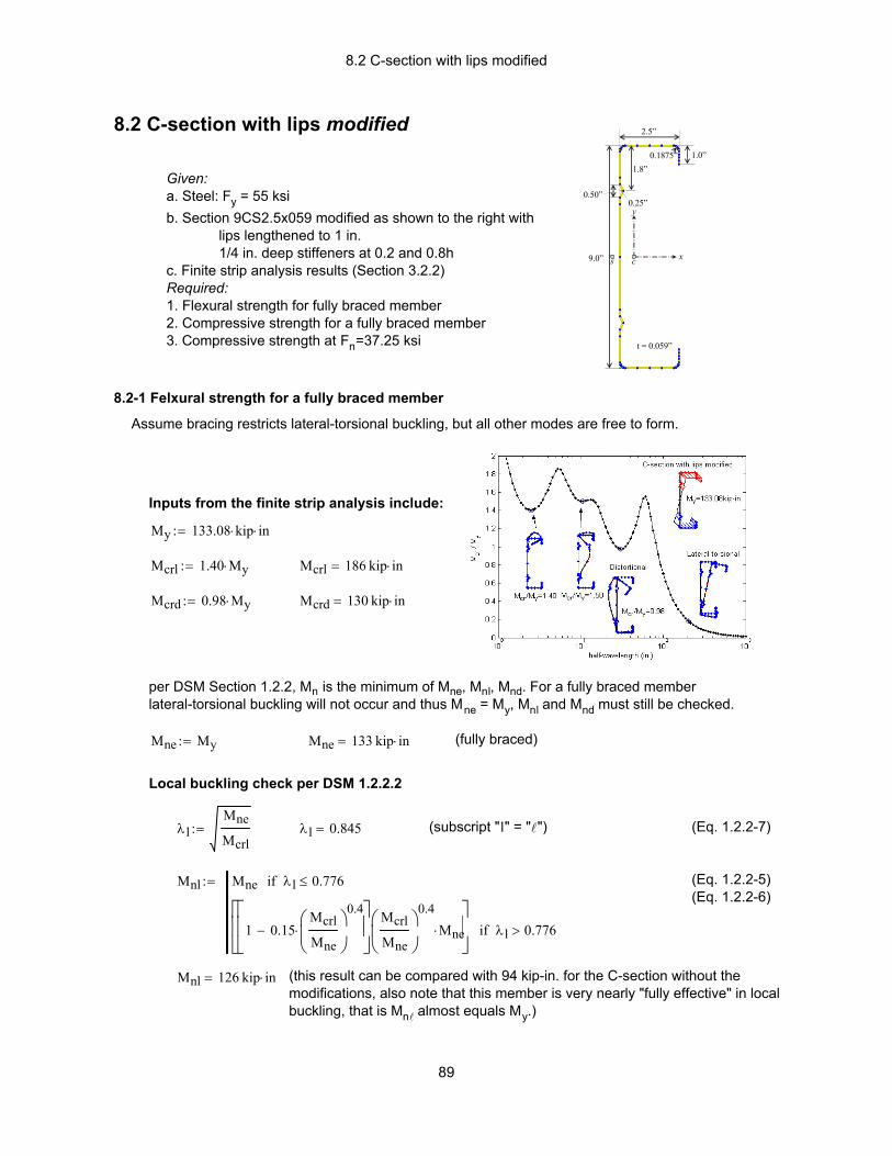
8.2 C-section with lips modified
(this result can be compared with 94 kip-in. for the C-section without the modifications, also note that this member is very nearly "fully effective" in local buckling, that is Mnl almost equals My.)
Mnl 126 kip in⋅=
(Eq. 1.2.2-5)(Eq. 1.2.2-6)
Mnl Mne λl 0.776≤if
1 0.15Mcrl
Mne
0.4
⋅−
Mcrl
Mne
0.4
Mne⋅
λl 0.776>if
:=
(Eq. 1.2.2-7)(subscript "l" = "l")λl 0.845=λlMne
Mcrl:=
Local buckling check per DSM 1.2.2.2
(fully braced)Mne 133 kip in⋅=Mne My:=
per DSM Section 1.2.2, Mn is the minimum of Mne, Mnl, Mnd. For a fully braced member lateral-torsional buckling will not occur and thus Mne = My, Mnl and Mnd must still be checked.
Mcrd 130 kip in⋅=Mcrd 0.98 My⋅:=
Mcrl 186 kip in⋅=Mcrl 1.40 My⋅:=
My 133.08 kip⋅ in⋅:=
Inputs from the finite strip analysis include:
Assume bracing restricts lateral-torsional buckling, but all other modes are free to form.
8.2-1 Felxural strength for a fully braced member
Given: a. Steel: Fy = 55 ksib. Section 9CS2.5x059 modified as shown to the right with
lips lengthened to 1 in.1/4 in. deep stiffeners at 0.2 and 0.8h
c. Finite strip analysis results (Section 3.2.2)Required:1. Flexural strength for fully braced member2. Compressive strength for a fully braced member3. Compressive strength at Fn=37.25 ksi
8.2 C-section with lips modified
9.0”
2.5”
1.0”
0.25”
1.8”0.1875”
t = 0.059”
x
y
cs
0.50”
89
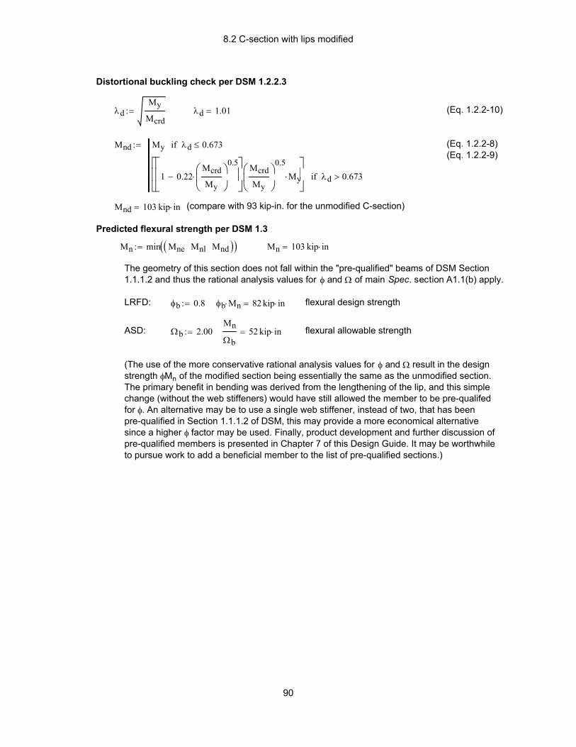
8.2 C-section with lips modified
(The use of the more conservative rational analysis values for φ and Ω result in the design strength φMn of the modified section being essentially the same as the unmodified section. The primary benefit in bending was derived from the lengthening of the lip, and this simple change (without the web stiffeners) would have still allowed the member to be pre-qualifed for φ. An alternative may be to use a single web stiffener, instead of two, that has been pre-qualified in Section 1.1.1.2 of DSM, this may provide a more economical alternative since a higher φ factor may be used. Finally, product development and further discussion of pre-qualified members is presented in Chapter 7 of this Design Guide. It may be worthwhile to pursue work to add a beneficial member to the list of pre-qualified sections.)
flexural allowable strengthMn
Ωb52 kip in⋅=Ωb 2.00:=ASD:
flexural design strengthφb Mn⋅ 82 kip in⋅=φb 0.8:=LRFD:
The geometry of this section does not fall within the "pre-qualified" beams of DSM Section 1.1.1.2 and thus the rational analysis values for φ and Ω of main Spec. section A1.1(b) apply.
Mn 103 kip in⋅=Mn min Mne Mnl Mnd( )( ):=
Predicted flexural strength per DSM 1.3
(compare with 93 kip-in. for the unmodified C-section)Mnd 103 kip in⋅=
(Eq. 1.2.2-8)(Eq. 1.2.2-9)
Mnd My λd 0.673≤if
1 0.22Mcrd
My
0.5
⋅−
Mcrd
My
0.5
My⋅
λd 0.673>if
:=
(Eq. 1.2.2-10)λd 1.01=λdMy
Mcrd:=
Distortional buckling check per DSM 1.2.2.3
90
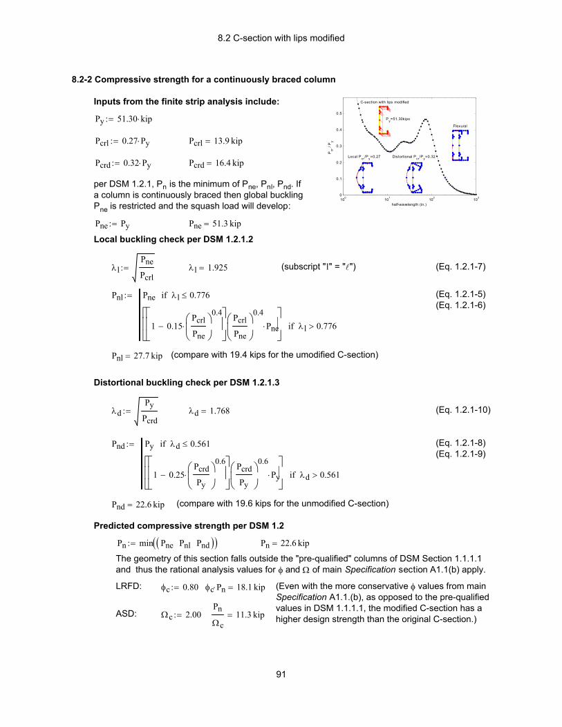
8.2 C-section with lips modified
Distortional buckling check per DSM 1.2.1.3
λdPy
Pcrd:= λd 1.768= (Eq. 1.2.1-10)
Pnd Py λd 0.561≤if
1 0.25Pcrd
Py
0.6
⋅−
Pcrd
Py
0.6
Py⋅
λd 0.561>if
:= (Eq. 1.2.1-8)(Eq. 1.2.1-9)
Pnd 22.6 kip= (compare with 19.6 kips for the unmodified C-section)
Predicted compressive strength per DSM 1.2
Pn min Pne Pnl Pnd( )( ):= Pn 22.6 kip=
The geometry of this section falls outside the "pre-qualified" columns of DSM Section 1.1.1.1 and thus the rational analysis values for φ and Ω of main Specification section A1.1(b) apply.
LRFD: φc 0.80:= φc Pn⋅ 18.1 kip= (Even with the more conservative φ values from main Specification A1.1.(b), as opposed to the pre-qualified values in DSM 1.1.1.1, the modified C-section has a higher design strength than the original C-section.)ASD: Ωc 2.00:=
Pn
Ωc11.3 kip=
8.2-2 Compressive strength for a continuously braced column
100 101 102 1030
0.1
0.2
0.3
0.4
0.5
half-wavelength (in.)
Pcr
/ P
y
C-section with lips modified
Py=51.30kips
Local Pcr/Py=0.27 Distortional Pcr/Py=0.32
Flexural
Inputs from the finite strip analysis include:
Py 51.30 kip⋅:=
Pcrl 0.27 Py⋅:= Pcrl 13.9 kip=
Pcrd 0.32 Py⋅:= Pcrd 16.4 kip=
per DSM 1.2.1, Pn is the minimum of Pne, Pnl, Pnd. If a column is continuously braced then global buckling Pne is restricted and the squash load will develop:
Pne Py:= Pne 51.3 kip=
Local buckling check per DSM 1.2.1.2
λlPne
Pcrl:= λl 1.925= (subscript "l" = "l") (Eq. 1.2.1-7)
Pnl Pne λl 0.776≤if
1 0.15Pcrl
Pne
0.4
⋅−
Pcrl
Pne
0.4
Pne⋅
λl 0.776>if
:= (Eq. 1.2.1-5)(Eq. 1.2.1-6)
Pnl 27.7 kip= (compare with 19.4 kips for the umodified C-section)
91
8.2 C-section with lips modified
Pn
Ωc10.8 kip=Ωc 2.00:=ASD:
(Note, the predicted design strength is well above the unmodifed C-section, predicted to have a nominal strength of only 12.9 kips.)
φc Pn⋅ 17.2 kip=φc 0.80:=LRFD:
The geometry of this section falls outside the "pre-qualified" columns of DSM Section 1.1.1.1 and thus the rational analysis values for φ and Ω of main Specification section A1.1(b) apply.
Pn 21.6 kip=Pn min Pne Pnl Pnd( )( ):=
Predicted compressive strength per DSM 1.2
identical to that calculated in Example 8.2-2Pnd 22.6 kip=
Distortional buckling check per DSM 1.2.1.3
(down from 27.7 kips when Pne=PY, but well above Pnl = 15.2 kips for the unmodified C-section.)
Pnl 21.6 kip=
(Eq. 1.2.1-5)(Eq. 1.2.1-6)
Pnl Pne λl 0.776≤if
1 0.15Pcrl
Pne
0.4
⋅−
Pcrl
Pne
0.4
Pne⋅
λl 0.776>if
:=
(Eq. 1.2.1-7)(subscript "l" = "l")λl 1.584=λlPne
Pcrl:=
Local buckling check per DSM 1.2.1.2
Note, Pne is slightly larger in this example than in Example 8.1-5 because the cross-sectional area of the modified C-section is larger.
Pne 34.7 kip=Pne Ag 37.25⋅ ksi⋅:=
Similar to Example 8.1-5 the strength of the column is calculated at a long column stress F n of 37.25 ksi. Per DSM Section 1.2.1, Pn is the minimum of Pne, Pnl, Pnd, and:
In Example 8.1-5 the compressive strength of an unmodified C-section at a uniform compressive stress of 37.25 ksi was considered. This stress was determined based on strong axis buckling at an unbraced length of 20 ft. as detailed in AISI (2002) Example III-1.
8.2-3 Compressive strength at Fn=37.25 ksi
92
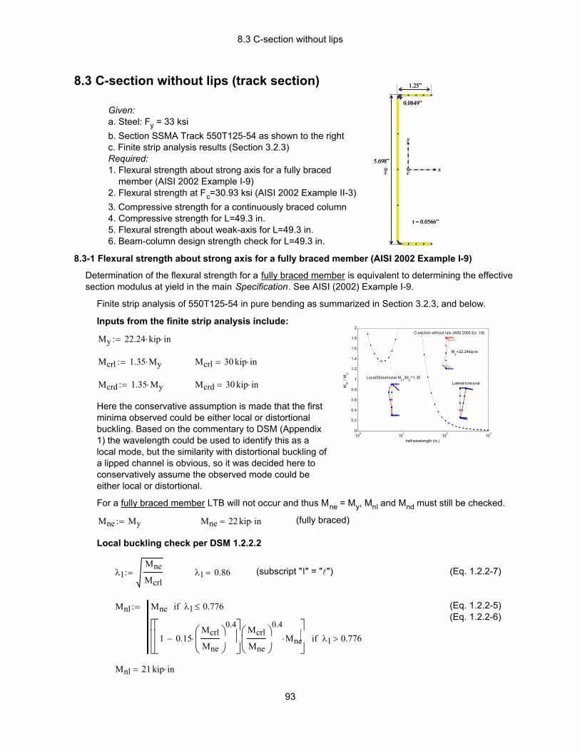
8.3 C-section without lips
Mnl 21 kip in⋅=
(Eq. 1.2.2-5)(Eq. 1.2.2-6)
Mnl Mne λl 0.776≤if
1 0.15Mcrl
Mne
0.4
⋅−
Mcrl
Mne
0.4
Mne⋅
λl 0.776>if
:=
(Eq. 1.2.2-7)(subscript "l" = "l")λl 0.86=λlMne
Mcrl:=
Local buckling check per DSM 1.2.2.2
(fully braced)Mne 22 kip in⋅=Mne My:=
For a fully braced member LTB will not occur and thus Mne = My, Mnl and Mnd must still be checked.
Here the conservative assumption is made that the first minima observed could be either local or distortional buckling. Based on the commentary to DSM (Appendix 1) the wavelength could be used to identify this as a local mode, but the similarity with distortional buckling of a lipped channel is obvious, so it was decided here to conservatively assume the observed mode could be either local or distortional.
Mcrd 30 kip in⋅=Mcrd 1.35 My⋅:=
Mcrl 30 kip in⋅=Mcrl 1.35 My⋅:=
My 22.24 kip⋅ in⋅:=
Inputs from the finite strip analysis include:
100 101 102 1030
0.2
0.4
0.6
0.8
1
1.2
1.4
1.6
1.8
2
half-wavelength (in.)
Mcr
/ M
y
C-section without lips (AISI 2002 Ex. I-9)
My=22.24kip-in.
Local/Distortional Mcr/My=1.35Lateral-torsional
Finite strip analysis of 550T125-54 in pure bending as summarized in Section 3.2.3, and below.
Determination of the flexural strength for a fully braced member is equivalent to determining the effectivesection modulus at yield in the main Specification. See AISI (2002) Example I-9.
8.3-1 Flexural strength about strong axis for a fully braced member (AISI 2002 Example I-9)
Given: a. Steel: Fy = 33 ksib. Section SSMA Track 550T125-54 as shown to the rightc. Finite strip analysis results (Section 3.2.3)Required:1. Flexural strength about strong axis for a fully braced member (AISI 2002 Example I-9)2. Flexural strength at Fc=30.93 ksi (AISI 2002 Example II-3)3. Compressive strength for a continuously braced column4. Compressive strength for L=49.3 in.5. Flexural strength about weak-axis for L=49.3 in.6. Beam-column design strength check for L=49.3 in.
8.3 C-section without lips (track section)
5.698”
1.25”
0.0849”
t = 0.0566”
x
y
cs
5.698”
1.25”
0.0849”
t = 0.0566”
x
y
cs
93
8.3 C-section without lips
flexural allowable strengthMn
Ωb10 kip in⋅=Ωb 2.00:=ASD:
flexural design strengthφb Mn⋅ 15 kip in⋅=φb 0.8:=LRFD:
The geometry of this section falls outside the "pre-qualified" beams of DSM 1.1.1.2 and thus the φ and Ω of the rational analysis clause of the main Specification, A1.1(b), must be used.
Mn 19 kip in⋅=Mn min Mne Mnl Mnd( )( ):=
Predicted flexural strength per 1.3
In this example the distortional buckling strength is only 2 kip-in. less than the local buckling strength, so the conservative assumption that the first minima might be considered either local or distortional is not overly detrimental to the economy of the design. If the (assumed) lateral bracing that is restricting LTB also restricts the flange movement, it would be reasonable to assume DB is restricted here as well, and thus Mnd=MY and Mnl would control. Further, since only local buckling interacts with LTB for longer lengths Mnl will control over Mnd regardless. Thus, the conservative assumption for Mcrd only has impact for intermediate lengths spans for which LTB is braced.
Mnd 19 kip in⋅=
(Eq. 1.2.2-8)(Eq. 1.2.2-9)
Mnd My λd 0.673≤if
1 0.22Mcrd
My
0.5
⋅−
Mcrd
My
0.5
My⋅
λd 0.673>if
:=
(Eq. 1.2.2-10)λd 0.86=λdMy
Mcrd:=
Distortional buckling check per DSM 1.2.2.3
94
8.3 C-section without lips
Note: For a long unbraced length lateral-torsional buckling (LTB) controls the strength of beams. In the main Specification interaction of local and lateral-torsional buckling is handled by calculating the maximum stress for LTB (e.g., Fc, Eq. C3.1.2.1-3) and then determining the effective section modulus, Se, at stress Fc. The maximum stress for LTB can be converted into a strength by mutliplying the stress Fc times the gross section modulus, i.e., Mne=SGFc. In DSM the local buckling equation then picks up this interaction by modifying the slenderness (DSM Eq.1.2.2-7) and the maximum capacity (DSM Eq.'s 1.2.2-5,6).
(fully braced)Mne 21 kip in⋅=Mne Sg 30.93⋅ ksi⋅:=Sg 0.67 in3=
To be consistent with the AISI (2002) Design Manual example base the lateral-torisonal buckling on strength Method (a) the stress Fc: Mne = SgFc. Note, Mnl and Mnd must still be checked.
Mne
Sg30.73 ksi=to compare with Fc divide by SgMne 20.71 kip in⋅=
(Eq. 1.2.2-3)
(Eq. 1.2.2-2)
(Eq. 1.2.2-1)Mne Mcre Mcre 0.56 My⋅<if
109
My⋅ 110 My⋅
36 Mcre⋅−
⋅
2.78 My⋅ Mcre≥ 0.56 My⋅≥if
My Mcre 2.78 My⋅>if
:=
Mcre
Sg56.63 ksi=to compare with Fe divide by Sg
8.3-2 Flexural strength for Fc=30.93 ksi (AISI 2002 Example II-3)
In AISI (2002) Example II-3 this track section is examined as a beam with a 72 in. simple span under uniform load, braced against twisting and lateral deflection at the ends and at midspan. Following main Specification Equations C3.1.2.1 AISI (2002) Example II-3 provides the elastic lateral-torsional buckling stress Fe and then the inelastic lateral-torsional buckling stress F c.
Method (a) per AISI (2002) Example II-3
Cb 1.30:= moment gradient modification factor for a half-span under uniform load (C3.1.2.1-10)
Fe Cb 36.48⋅ ksi⋅:= Fe 47.42 ksi= determined via C3.1.2.1-5
Fc 30.93 ksi⋅:= determined via C3.1.2.1-3
Method (b) from finite strip analysis
Mcre 1.32 My⋅:= direct from finite strip analysis at a half-wavelength of 36 in., see Section 3.2.3
Mcre Cb Mcre⋅:= Cb of the main Spec. applies, and Mcre 38.16 kip in⋅=
95
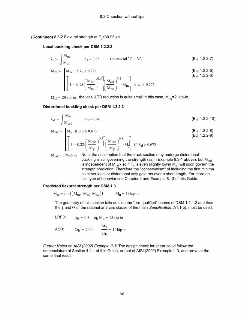
8.3 C-section without lips
Further Notes on AISI (2002) Example II-3: The design check for shear could follow the nomenclature of Section 4.4.1 of this Guide, or that of AISI (2002) Example II-3, and arrive at the same final result.
Mn
Ωb10 kip in⋅=Ωb 2.00:=ASD:
φb Mn⋅ 15 kip in⋅=φb 0.8:=LRFD:
The geometry of this section falls outside the "pre-qualified" beams of DSM 1.1.1.2 and thus the φ and Ω of the rational analysis clause of the main Specification, A1.1(b), must be used.
Mn 19 kip in⋅=Mn min Mne Mnl Mnd( )( ):=
Predicted flexural strength per DSM 1.3
Note, the assumption that the track section may undergo distortional buckling is still governing the strength (as in Example 8.3-1 above), but M nd is independent of Mne - so if Fc is even slightly lower Mnl will soon govern the strength prediction. Therefore the "conservatism" of including the first minima as either local or distortional only governs over a short length. For more on this type of behavior see Chapter 4 and Example 8.13 of this Guide.
Mnd 19 kip in⋅=
(Eq. 1.2.2-8)(Eq. 1.2.2-9)
Mnd My λd 0.673≤if
1 0.22Mcrd
My
0.5
⋅−
Mcrd
My
0.5
My⋅
λd 0.673>if
:=
(Eq. 1.2.2-10)λd 0.86=λdMy
Mcrd:=
Distortional buckling check per DSM 1.2.2.3
the local-LTB reduction is quite small in this case, Mne=21kip-in.Mnl 20 kip in⋅=
(Eq. 1.2.2-5)(Eq. 1.2.2-6)
Mnl Mne λl 0.776≤if
1 0.15Mcrl
Mne
0.4
⋅−
Mcrl
Mne
0.4
Mne⋅
λl 0.776>if
:=
(Eq. 1.2.2-7)(subscript "l" = "l")λl 0.83=λlMne
Mcrl:=
Local buckling check per DSM 1.2.2.2
(Continued) 8.3-2 Flexural strength at Fc=30.93 ksi
96
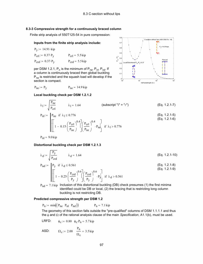
8.3 C-section without lips
Pnl 9.0 kip=
Distortional buckling check per DSM 1.2.1.3
λdPy
Pcrd:= λd 1.64= (Eq. 1.2.1-10)
Pnd Py λd 0.561≤if
1 0.25Pcrd
Py
0.6
⋅−
Pcrd
Py
0.6
Py⋅
λd 0.561>if
:= (Eq. 1.2.1-8)(Eq. 1.2.1-9)
Pnd 7.1 kip= Inclusion of this distortional buckling (DB) check presumes (1) the first minima identified could be DB or local, (2) the bracing that is restricting long column buckling is not restricting DB.
Predicted compressive strength per DSM 1.2
Pn min Pne Pnl Pnd( )( ):= Pn 7.1 kip=
The geometry of this section falls outside the "pre-qualified" columns of DSM 1.1.1.1 and thus the φ and Ω of the rational analysis clause of the main Specification, A1.1(b), must be used.
LRFD: φc 0.80:= φc Pn⋅ 5.7 kip=
ASD: Ωc 2.00:=Pn
Ωc3.5 kip=
8.3-3 Compressive strength for a continuously braced column
100 101 102 1030
0.1
0.2
0.3
0.4
0.5
0.6
0.7
0.8
half-wavelength (in.)
Pcr
/ P
y
C-section without lips (AISI 2002 Ex. I-8)
Py=14.91kips
Local/Distortional Pcr/Py=0.37
Flexural
Finite strip analysis of 550T125-54 in pure compression:
Inputs from the finite strip analysis include:
Py 14.91 kip⋅:=
Pcrl 0.37 Py⋅:= Pcrl 5.5 kip=
Pcrd 0.37 Py⋅:= Pcrd 5.5 kip=
per DSM 1.2.1, Pn is the minimum of Pne, Pnl, Pnd. If a column is continuously braced then global buckling Pne is restricted and the squash load will develop if the section is compact.
Pne Py:= Pne 14.9 kip=
Local buckling check per DSM 1.2.1.2
λlPne
Pcrl:= λl 1.64= (subscript "l" = "l") (Eq. 1.2.1-7)
Pnl Pne λl 0.776≤if
1 0.15Pcrl
Pne
0.4
⋅−
Pcrl
Pne
0.4
Pne⋅
λl 0.776>if
:= (Eq. 1.2.1-5)(Eq. 1.2.1-6)
97
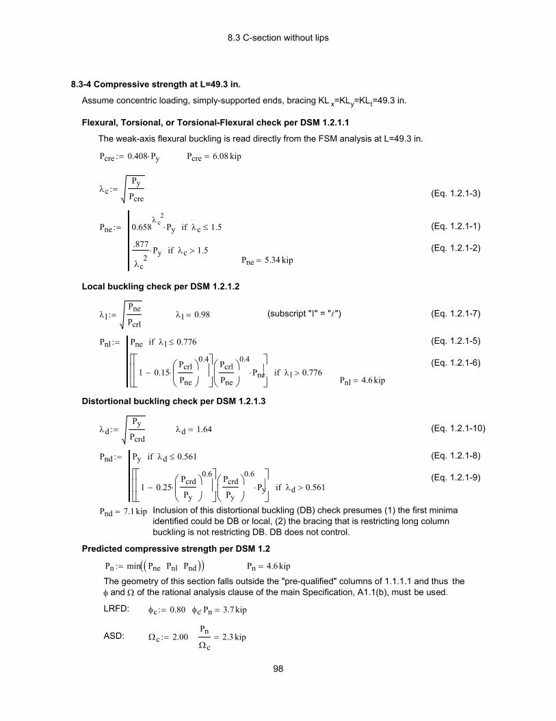
8.3 C-section without lips
Pnl 4.6 kip=
Distortional buckling check per DSM 1.2.1.3
λdPy
Pcrd:= λd 1.64= (Eq. 1.2.1-10)
Pnd Py λd 0.561≤if
1 0.25Pcrd
Py
0.6
⋅−
Pcrd
Py
0.6
Py⋅
λd 0.561>if
:= (Eq. 1.2.1-8)
(Eq. 1.2.1-9)
Pnd 7.1 kip= Inclusion of this distortional buckling (DB) check presumes (1) the first minima identified could be DB or local, (2) the bracing that is restricting long column buckling is not restricting DB. DB does not control.
Predicted compressive strength per DSM 1.2
Pn min Pne Pnl Pnd( )( ):= Pn 4.6 kip=
The geometry of this section falls outside the "pre-qualified" columns of 1.1.1.1 and thus the φ and Ω of the rational analysis clause of the main Specification, A1.1(b), must be used.
LRFD: φc 0.80:= φc Pn⋅ 3.7 kip=
ASD: Ωc 2.00:=Pn
Ωc2.3 kip=
8.3-4 Compressive strength at L=49.3 in.
Assume concentric loading, simply-supported ends, bracing KL x=KLy=KLt=49.3 in.
Flexural, Torsional, or Torsional-Flexural check per DSM 1.2.1.1
The weak-axis flexural buckling is read directly from the FSM analysis at L=49.3 in.
Pcre 0.408 Py⋅:= Pcre 6.08 kip=
λcPy
Pcre:= (Eq. 1.2.1-3)
Pne 0.658λ c
2
Py⋅ λc 1.5≤if
.877
λc2
Py⋅ λc 1.5>if
:= (Eq. 1.2.1-1)
(Eq. 1.2.1-2)Pne 5.34 kip=
Local buckling check per DSM 1.2.1.2
λlPne
Pcrl:= λl 0.98= (subscript "l" = "l") (Eq. 1.2.1-7)
Pnl Pne λl 0.776≤if
1 0.15Pcrl
Pne
0.4
⋅−
Pcrl
Pne
0.4
Pne⋅
λl 0.776>if
:= (Eq. 1.2.1-5)
(Eq. 1.2.1-6)
98
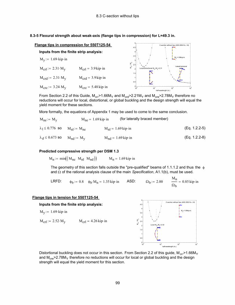
8.3 C-section without lips
so Mnd My:= Mnd 1.69 kip in⋅= (Eq. 1.2.2-8)
Predicted compressive strength per DSM 1.3
Mn min Mne Mnl Mnd( )( ):= Mn 1.69 kip in⋅=
The geometry of this section falls outside the "pre-qualified" beams of 1.1.1.2 and thus the φ and Ω of the rational analysis clause of the main Specification, A1.1(b), must be used.
LRFD: φb 0.8:= φb Mn⋅ 1.35 kip in⋅= ASD: Ωb 2.00:=Mn
Ωb0.85 kip in⋅=
100 101 102 1030
0.5
1
1.5
2
2.5
3
3.5
4
4.5
5
half-wavelength (in.)
Mcr
/ M
y
C-section without lips (AISI 2002 Ex. I-9)
My=1.69kip-in.
Local Mcr/My=2.52
Flange tips in tension for 550T125-54
Inputs from the finite strip analysis:
My 1.69 kip⋅ in⋅:=
Mcrl 2.52 My⋅:= Mcrl 4.26 kip in⋅=
Distortional buckling does not occur in this section. From Section 2.2 of this guide, Mcrl>1.66MY and Mcre>2.78MY therefore no reductions will occur for local or global buckling and the design strength will equal the yield moment for this section.
8.3-5 Flexural strength about weak-axis (flange tips in compression) for L=49.3 in.
100 101 102 1030
0.5
1
1.5
2
2.5
3
3.5
4
4.5
5
half-wavelength (in.)
Mcr
/ M
y
C-section without lips (AISI 2002 Ex. I-9)
My=1.69kip-in.
Local/Distortional Mcr/My=2.31Lateral-torsional
Flange tips in compression for 550T125-54
Inputs from the finite strip analysis:
My 1.69 kip⋅ in⋅:=
Mcrl 2.31 My⋅:= Mcrl 3.9 kip in⋅=
Mcrd 2.31 My⋅:= Mcrd 3.9 kip in⋅=
Mcre 3.24 My⋅:= Mcre 5.48 kip in⋅=
From Section 2.2 of this Guide, Mcrl>1.66MY and Mcrd>2.21MY and Mcre>2.78MY therefore no reductions will occur for local, distortional, or global buckling and the design strength will equal the yield moment for these sections.
More formally, the equations of Appendix 1 may be used to come to the same conclusion.
Mne My:= Mne 1.69 kip in⋅= (for laterally braced member)
λl 0.776≤ so Mnl Mne:= Mnl 1.69 kip in⋅= (Eq. 1.2.2-5)
λd 0.673≤
99
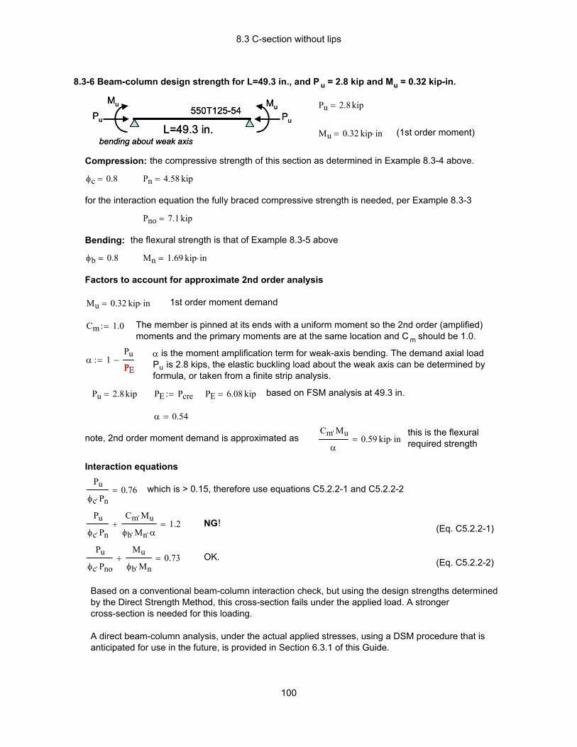
8.3 C-section without lips
Pu 2.8 kip= PE Pcre:= PE 6.08 kip= based on FSM analysis at 49.3 in.
α 0.54=
this is the flexural required strengthnote, 2nd order moment demand is approximated as
Cm Mu⋅
α0.59 kip in⋅=
Interaction equationsPu
φc Pn⋅0.76= which is > 0.15, therefore use equations C5.2.2-1 and C5.2.2-2
Pu
φc Pn⋅
Cm Mu⋅
φb Mn⋅ α⋅+ 1.2= NG! (Eq. C5.2.2-1)
Pu
φc Pno⋅
Mu
φb Mn⋅+ 0.73= OK. (Eq. C5.2.2-2)
Based on a conventional beam-column interaction check, but using the design strengths determined by the Direct Strength Method, this cross-section fails under the applied load. A stronger cross-section is needed for this loading.
A direct beam-column analysis, under the actual applied stresses, using a DSM procedure that is anticipated for use in the future, is provided in Section 6.3.1 of this Guide.
8.3-6 Beam-column design strength for L=49.3 in., and P u = 2.8 kip and Mu = 0.32 kip-in.
Pu
Mu
Pu
Mu
L=49.3 in.
550T125-54
bending about weak axis
Pu
Mu
Pu
Mu
L=49.3 in.
550T125-54
bending about weak axis
Pu 2.8 kip=
Mu 0.32 kip in⋅= (1st order moment)
Compression: the compressive strength of this section as determined in Example 8.3-4 above.
φc 0.8= Pn 4.58 kip=
for the interaction equation the fully braced compressive strength is needed, per Example 8.3-3
Pno 7.1 kip=
Bending: the flexural strength is that of Example 8.3-5 above
φb 0.8= Mn 1.69 kip in⋅=
Factors to account for approximate 2nd order analysis
Mu 0.32 kip in⋅= 1st order moment demand
Cm 1.0:= The member is pinned at its ends with a uniform moment so the 2nd order (amplified) moments and the primary moments are at the same location and C m should be 1.0.
α is the moment amplification term for weak-axis bending. The demand axial load Pu is 2.8 kips, the elastic buckling load about the weak axis can be determined by formula, or taken from a finite strip analysis.
α 1Pu
PE−:=
PE
100

8.4 C-section without lips modified
Mnl 23 kip in⋅= (Eq. 1.2.2-5)
Distortional buckling check per DSM 1.2.2.3
λdMy
Mcrd:= λd 0.69= (Eq. 1.2.2-10)
Mnd My λd 0.673≤if
1 0.22Mcrd
My
0.5
⋅−
Mcrd
My
0.5
My⋅
λd 0.673>if
:= (Eq. 1.2.2-8)(Eq. 1.2.2-9)
Mnd 22 kip in⋅= The DB reduction from My is small. Strength is improved from Example 8.3-1
Predicted flexural strength per DSM 1.3 Mn min Mne Mnl Mnd( )( ):= Mn 22 kip in⋅=
The geometry of this section falls outside the "pre-qualified" beams of DSM 1.1.1.2 and thus the φ and Ω of the rational analysis clause of the main Specification, A1.1(b), must be used.
LRFD: φb 0.8:= φb Mn⋅ 18 kip in⋅= ASD: Ωb 2.00:=
5.698”
1.25”
0.0849”
t = 0.0566”
x
y
cs
0.12”
0.55”
5.698”
1.25”
0.0849”
t = 0.0566”
x
y
cs
0.12”
0.55”
8.4 C-section without lips modified (track section)Given: a. Steel: Fy = 33 ksib. Modified Section SSMA Track 550T125-54
- stiffener added to the flanges as shownc. Finite strip analysis results (Section 3.2.4)Required:1. Flexural strength about strong axis for a fully braced member2. Compressive strength for a continuously braced column
8.4-1 Flexural strength about strong axis for a fully braced member
Finite strip analysis of modified 550T125-54 in pure bending is summarized in Section 3.2.4 and below.
100 101 102 1030
0.5
1
1.5
2
2.5
3
half-wavelength (in.)
Mcr
/ M
y
C-section without lips modified
My=22.55kip-in.
Local/Distortional Mcr/My=2.13Lateral-torsional
Inputs from the finite strip analysis include:
My 22.55 kip⋅ in⋅:=
Mcrl 2.13 My⋅:= Mcrl 48 kip in⋅=
Mcrd 2.13 My⋅:= Mcrd 48 kip in⋅=
Similar to Example 8.3 the conservative assumption is again made that the first minima observed could be either local or distortional buckling.
For a fully braced member LTB will not occur and thus Mne = My, Mnl and Mnd must still be checked.
Mne My:= Mne 23 kip in⋅= (fully braced)
Local buckling check per DSM 1.2.2.2
per Sec. 2.2 of this Guide, since Mcrl>1.66My Mnl Mne:=
101

8.4 C-section without lips modified
Distortional buckling check per DSM 1.2.1.3
λdPy
Pcrd:= λd 1.49= (Eq. 1.2.1-10)
Pnd Py λd 0.561≤if
1 0.25Pcrd
Py
0.6
⋅−
Pcrd
Py
0.6
Py⋅
λd 0.561>if
:= (Eq. 1.2.1-8)(Eq. 1.2.1-9)
Pnd 8.0 kip= Inclusion of this distortional buckling (DB) check presumes (1) the first minima identified could be DB or local, (2) the bracing which is restricting long column buckling is not restricting DB.
Predicted compressive strength per DSM 1.2
Pn min Pne Pnl Pnd( )( ):= Pn 7.98 kip=
The geometry of this section falls outside the "pre-qualified" columns of DSM 1.1.1.1 and thus the φ and Ω of the rational analysis clause, main Specification A1.1(b), must be used.
LRFD: φc 0.80:= φc Pn⋅ 6.4 kip= compressive design strength
ASD: Ωc 2.00:=Pn
Ωc4 kip= compressive allowable strength
8.4-2 Compressive strength for a continuously braced column
Finite strip analysis of modified 550T125-54 in compression as summarized in Section 3.2.4
100 101 102 1030
0.1
0.2
0.3
0.4
0.5
0.6
0.7
0.8
half-wavelength (in.)
Pcr
/ P
y
C-section without lips modified
Py=15.25kips
Local/Distortional Pcr/Py=0.45
Flexural
Inputs from the finite strip analysis include:Py 15.25 kip⋅:=
Pcrl 0.45 Py⋅:= Pcrl 6.9 kip=
Pcrd 0.45 Py⋅:= Pcrd 6.9 kip=
per DSM 1.2.1, Pn is the minimum of Pne, Pnl, Pnd. Assume the column is continuously braced against global buckling, then the global column strength Pne is the squash load.
Pne Py:= Pne 15.2 kip=
Local buckling check per DSM 1.2.1.2
λlPne
Pcrl:= λl 1.49= (subscript "l" = "l") (Eq. 1.2.1-7)
Pnl Pne λl 0.776≤if
1 0.15Pcrl
Pne
0.4
⋅−
Pcrl
Pne
0.4
Pne⋅
λl 0.776>if
:= (Eq. 1.2.1-5)(Eq. 1.2.1-6)
Pnl 9.9 kip=
102
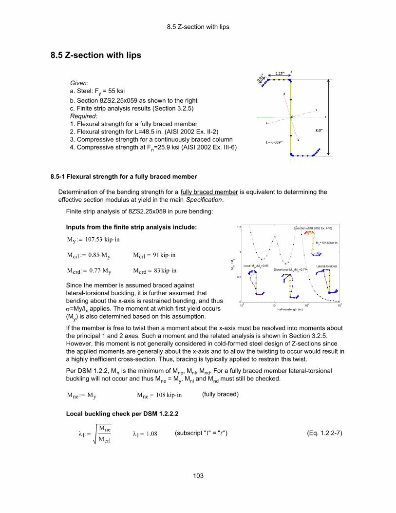
8.5 Z-section with lips
(Eq. 1.2.2-7)(subscript "l" = "l")λl 1.08=λlMne
Mcrl:=
Local buckling check per DSM 1.2.2.2
(fully braced)Mne 108 kip in⋅=Mne My:=
Per DSM 1.2.2, Mn is the minimum of Mne, Mnl, Mnd. For a fully braced member lateral-torsional buckling will not occur and thus Mne = My, Mnl and Mnd must still be checked.
If the member is free to twist then a moment about the x-axis must be resolved into moments about the principal 1 and 2 axes. Such a moment and the related analysis is shown in Section 3.2.5. However, this moment is not generally considered in cold-formed steel design of Z-sections since the applied moments are generally about the x-axis and to allow the twisting to occur would result in a highly inefficient cross-section. Thus, bracing is typically applied to restrain this twist.
Since the member is assumed braced against lateral-torsional buckling, it is further assumed that bending about the x-axis is restrained bending, and thus σ=My/Ix applies. The moment at which first yield occurs (My) is also determined based on this assumption.
Mcrd 83 kip in⋅=Mcrd 0.77 My⋅:=
Mcrl 91 kip in⋅=Mcrl 0.85 My⋅:=
My 107.53 kip⋅ in⋅:=
Inputs from the finite strip analysis include:
100 101 102 1030
0.5
1
1.5
half-wavelength (in.)
Mcr
/ M
y Z-section (AISI 2002 Ex. I-10)
My=107.53kip-in.
Local Mcr/My=0.85Distortional Mcr/My=0.77
Lateral-torsional
Finite strip analysis of 8ZS2.25x059 in pure bending:
Determination of the bending strength for a fully braced member is equivalent to determining the effective section modulus at yield in the main Specification.
8.5-1 Flexural strength for a fully braced member
Given: a. Steel: Fy = 55 ksib. Section 8ZS2.25x059 as shown to the rightc. Finite strip analysis results (Section 3.2.5)Required:1. Flexural strength for a fully braced member2. Flexural strength for L=48.5 in. (AISI 2002 Ex. II-2)3. Compressive strength for a continuously braced column4. Compressive strength at Fn=25.9 ksi (AISI 2002 Ex. III-6)
C x
y
1
1
2
2
8.0”
2.25”
t = 0.059”
0.91”
C x
y
1
1
2
2
8.0”
2.25”
t = 0.059”
0.91”
8.5 Z-section with lips
103

8.5 Z-section with lips
The geometry of this cross-section falls within the "pre-qualified" beams of DSM 1.1.1.2 and the higher φ and lower Ω of DSM section 1.2.2 may therefore be used.
LRFD: φb 0.9:= φb Mn⋅ 69 kip in⋅= flexural design strength
ASD: Ωb 1.67:=Mn
Ωb46 kip in⋅= flexural allowable strength
Note on uplift
Part 4 of AISI (2002) Design Manual Example II-2 calculates the strength of this cross-section in uplift. The formula is RSeFY, where SeFY is the fully braced flexural strength and R is an empirical factor from main Specification C3.1.3. If the conditions of C3.1.3 are met, strength in uplift can be found in this simple manner. For this example R=0.7
uplift: R 0.7:= R Mn⋅ 53.3 kip in⋅= nominal strength in uplift
The calibration of R factors was performed to the main Specification. The main Specification does not include an explicit check for distortional buckling. Therefore, if distortional buckling (M nd) controls the strength, the uplift prediction using R may be excessively conservative. In this case Mnd does control the strength (Mnl is considerably higher) thus this prediction is expected to be conservative. Arguably, a more accurate prediction would be RMnl. As discussed in Section 3.3.7 of this Guide, it is possible to have the elastic buckling analysis include the influence of restraints such as deck - direct calculation instead of a reliance on empiricial R factors would be the result.
(Continued) 8.5-1 Flexural strength for a fully braced member
Local buckling check per DSM 1.2.2.2 (continued)
Mnl Mne λl 0.776≤if
1 0.15Mcrl
Mne
0.4
⋅−
Mcrl
Mne
0.4
Mne⋅
λl 0.776>if
:= (Eq. 1.2.2-5)(Eq. 1.2.2-6)
Mnl 87 kip in⋅=
Distortional buckling check per DSM 1.2.2.3
λdMy
Mcrd:= λd 1.14= (Eq. 1.2.2-10)
Mnd My λd 0.673≤if
1 0.22Mcrd
My
0.5
⋅−
Mcrd
My
0.5
My⋅
λd 0.673>if
:= (Eq. 1.2.2-8)(Eq. 1.2.2-9)
Mnd 76 kip in⋅= distortional buckling readily controls the strength of this section.
Predicted flexural strength per DSM 1.3
Mn min Mne Mnl Mnd( )( ):= Mn 76 kip in⋅=
104
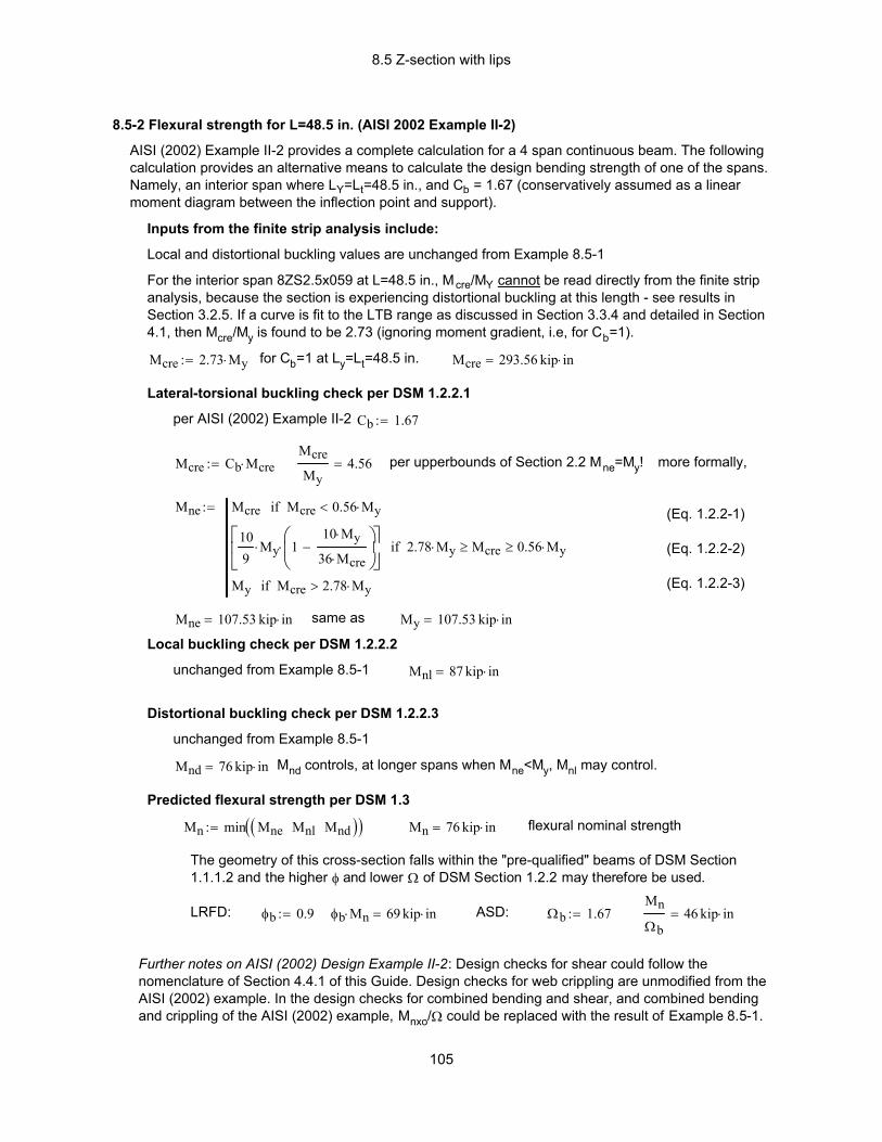
8.5 Z-section with lips
My 107.53 kip in⋅=
Local buckling check per DSM 1.2.2.2
unchanged from Example 8.5-1 Mnl 87 kip in⋅=
Distortional buckling check per DSM 1.2.2.3
unchanged from Example 8.5-1
Mnd 76 kip in⋅= Mnd controls, at longer spans when Mne<My, Mnl may control.
Predicted flexural strength per DSM 1.3
Mn min Mne Mnl Mnd( )( ):= Mn 76 kip in⋅= flexural nominal strength
The geometry of this cross-section falls within the "pre-qualified" beams of DSM Section 1.1.1.2 and the higher φ and lower Ω of DSM Section 1.2.2 may therefore be used.
LRFD: φb 0.9:= φb Mn⋅ 69 kip in⋅= ASD: Ωb 1.67:=Mn
Ωb46 kip in⋅=
Further notes on AISI (2002) Design Example II-2: Design checks for shear could follow the nomenclature of Section 4.4.1 of this Guide. Design checks for web crippling are unmodified from the AISI (2002) example. In the design checks for combined bending and shear, and combined bending and crippling of the AISI (2002) example, Mnxo/Ω could be replaced with the result of Example 8.5-1.
8.5-2 Flexural strength for L=48.5 in. (AISI 2002 Example II-2)
AISI (2002) Example II-2 provides a complete calculation for a 4 span continuous beam. The following calculation provides an alternative means to calculate the design bending strength of one of the spans. Namely, an interior span where LY=Lt=48.5 in., and Cb = 1.67 (conservatively assumed as a linear moment diagram between the inflection point and support).
Inputs from the finite strip analysis include:
Local and distortional buckling values are unchanged from Example 8.5-1
For the interior span 8ZS2.5x059 at L=48.5 in., Mcre/MY cannot be read directly from the finite strip analysis, because the section is experiencing distortional buckling at this length - see results in Section 3.2.5. If a curve is fit to the LTB range as discussed in Section 3.3.4 and detailed in Section 4.1, then Mcre/My is found to be 2.73 (ignoring moment gradient, i.e, for Cb=1).
Mcre 2.73 My⋅:= for Cb=1 at Ly=Lt=48.5 in. Mcre 293.56 kip in⋅=
Lateral-torsional buckling check per DSM 1.2.2.1
per AISI (2002) Example II-2 Cb 1.67:=
Mcre Cb Mcre⋅:=Mcre
My4.56= per upperbounds of Section 2.2 Mne=My! more formally,
Mne Mcre Mcre 0.56 My⋅<if
109
My⋅ 110 My⋅
36 Mcre⋅−
⋅
2.78 My⋅ Mcre≥ 0.56 My⋅≥if
My Mcre 2.78 My⋅>if
:= (Eq. 1.2.2-1)
(Eq. 1.2.2-2)
(Eq. 1.2.2-3)
Mne 107.53 kip in⋅= same as
105
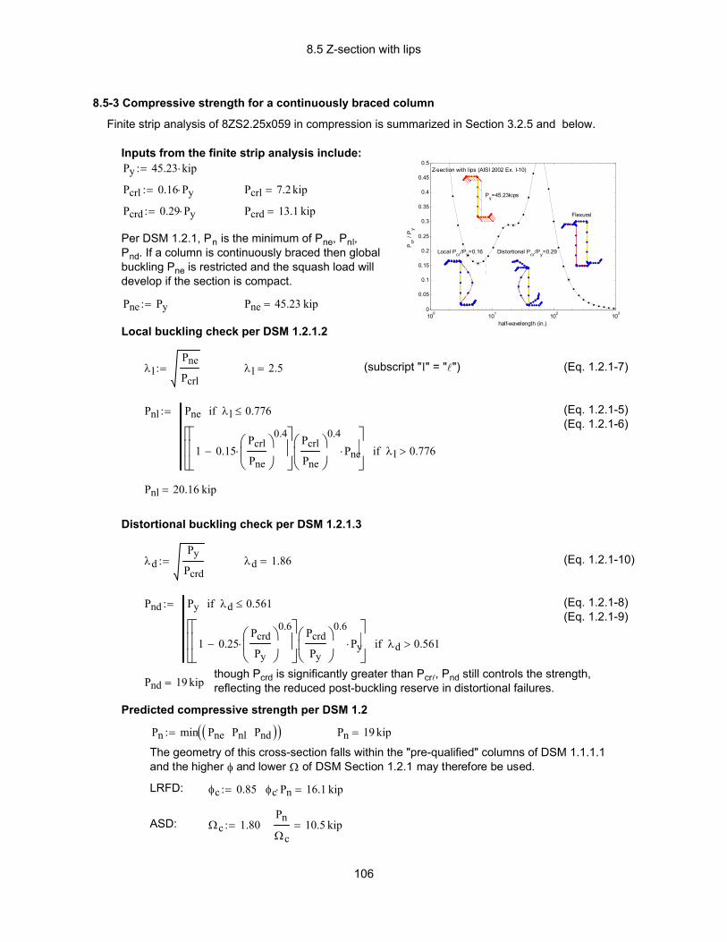
8.5 Z-section with lips
Pnl 20.16 kip=
Distortional buckling check per DSM 1.2.1.3
λdPy
Pcrd:= λd 1.86= (Eq. 1.2.1-10)
Pnd Py λd 0.561≤if
1 0.25Pcrd
Py
0.6
⋅−
Pcrd
Py
0.6
Py⋅
λd 0.561>if
:= (Eq. 1.2.1-8)(Eq. 1.2.1-9)
though Pcrd is significantly greater than Pcrl, Pnd still controls the strength, reflecting the reduced post-buckling reserve in distortional failures. Pnd 19 kip=
Predicted compressive strength per DSM 1.2
Pn min Pne Pnl Pnd( )( ):= Pn 19 kip=
The geometry of this cross-section falls within the "pre-qualified" columns of DSM 1.1.1.1 and the higher φ and lower Ω of DSM Section 1.2.1 may therefore be used.
LRFD: φc 0.85:= φc Pn⋅ 16.1 kip=
ASD: Ωc 1.80:=Pn
Ωc10.5 kip=
8.5-3 Compressive strength for a continuously braced column
Finite strip analysis of 8ZS2.25x059 in compression is summarized in Section 3.2.5 and below.
100 101 102 1030
0.05
0.1
0.15
0.2
0.25
0.3
0.35
0.4
0.45
0.5
half-wavelength (in.)
Pcr
/ P
y
Z-section with lips (AISI 2002 Ex. I-10)
Py=45.23kips
Local Pcr/Py=0.16 Distortional Pcr/Py=0.29
Flexural
Inputs from the finite strip analysis include:Py 45.23 kip⋅:=
Pcrl 0.16 Py⋅:= Pcrl 7.2 kip=
Pcrd 0.29 Py⋅:= Pcrd 13.1 kip=
Per DSM 1.2.1, Pn is the minimum of Pne, Pnl, Pnd. If a column is continuously braced then global buckling Pne is restricted and the squash load will develop if the section is compact.
Pne Py:= Pne 45.23 kip=
Local buckling check per DSM 1.2.1.2
λlPne
Pcrl:= λl 2.5= (subscript "l" = "l") (Eq. 1.2.1-7)
Pnl Pne λl 0.776≤if
1 0.15Pcrl
Pne
0.4
⋅−
Pcrl
Pne
0.4
Pne⋅
λl 0.776>if
:= (Eq. 1.2.1-5)(Eq. 1.2.1-6)
106
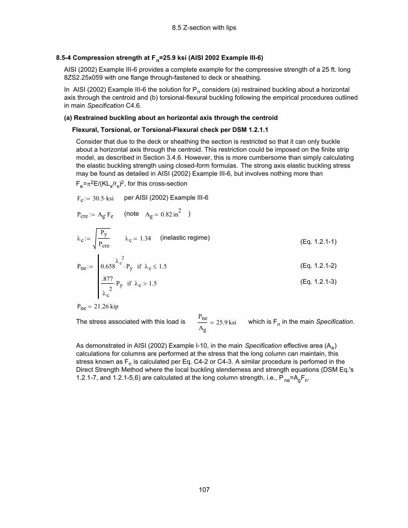
8.5 Z-section with lips
As demonstrated in AISI (2002) Example I-10, in the main Specification effective area (Ae) calculations for columns are performed at the stress that the long column can maintain, this stress known as Fn is calculated per Eq. C4-2 or C4-3. A similar procedure is perfomed in the Direct Strength Method where the local buckling slenderness and strength equations (DSM Eq.'s 1.2.1-7, and 1.2.1-5,6) are calculated at the long column strength, i.e., P ne=AgFn.
which is Fn in the main Specification.Pne
Ag25.9 ksi=The stress associated with this load is
Pne 21.26 kip=
(Eq. 1.2.1-3)
(Eq. 1.2.1-2)Pne 0.658λ c
2
Py⋅ λc 1.5≤if
.877
λc2
Py⋅ λc 1.5>if
:=
(Eq. 1.2.1-1)(inelastic regime)λc 1.34=λcPy
Pcre:=
)Ag 0.82 in2=(notePcre Ag Fe⋅:=
per AISI (2002) Example III-6Fe 30.5 ksi⋅:=
Consider that due to the deck or sheathing the section is restricted so that it can only buckle about a horizontal axis through the centroid. This restriction could be imposed on the finite strip model, as described in Section 3.4.6. However, this is more cumbersome than simply calculating the elastic buckling strength using closed-form formulas. The strong axis elastic buckling stress may be found as detailed in AISI (2002) Example III-6, but involves nothing more than Fe=π2E/(KLx/rx)2, for this cross-section
Flexural, Torsional, or Torsional-Flexural check per DSM 1.2.1.1
(a) Restrained buckling about an horizontal axis through the centroid
In AISI (2002) Example III-6 the solution for Pn considers (a) restrained buckling about a horizontal axis through the centroid and (b) torsional-flexural buckling following the empirical procedures outlined in main Specification C4.6.
AISI (2002) Example III-6 provides a complete example for the compressive strength of a 25 ft. long 8ZS2.25x059 with one flange through-fastened to deck or sheathing.
8.5-4 Compression strength at Fn=25.9 ksi (AISI 2002 Example III-6)
107

8.5 Z-section with lips
The impact of partial restraint on buckling modes is discussed in Section 3.4.7. The finite strip analysis to the right shows a key aspect of this discussion - restraint of a flange in compression can have a significant positive impact on distortional buckling. If the stiffness of the deck or sheathing can be reliably known, then inclusion of its stiffness directly in the finite strip model is possible. Appropriate modeling for compression members is also possible, but not included here.
AISI (2002) Example III-6 part 2 provides the solution using Specification equations of C4.6. The predicted capacity, Pn is 11.8 kips by this method.
Z-section (AISI 2002 Ex. I-10)
My=107.53kip-in.
Local Mcr/My=0.85Distortional Mcr/My=0.77
Lateral-torsional
100 101 102 1030
0.2
0.4
0.6
0.8
1
1.2
1.4
1.6
1.8
2
half-wavelength (in.)
Mcr
/ M
y
Z-section
My=107.53kip-in.
Local Mcr/My=0.85 Distortional Mcr/My=1.30
due tokφ
kφ
0.7 kip-in./rad/in.
(b) Torsional-flexural buckling via the empirical procedures of main Specification C4.6
Pn
Ωc6.9 kip=Ωc 1.80:=ASD:
φc Pn⋅ 10.6 kip=φc 0.85:=LRFD:
The geometry of this cross-section falls within the "pre-qualified" columns of DSM 1.1.1.1 and the higher φ and lower Ω of DSM Section 1.2.1 may therefore be used.
Pn 12.5 kip=Pn min Pne Pnl Pnd( )( ):=
Predicted compressive strength per DSM 1.2
(note, the distortional buckling prediction is the same as Example 8.5-2, and now no longer controls the predicted strength)
Pnd 19 kip=
(Continued) 8.5-4 Compressive strength at Fn=25.9 ksi (AISI 2002 Example III-6)
Local buckling check per DSM 1.2.1.2
(compare with λl of 2.5 for the same column with continuous bracing, see Example 8.5-2)
λlPne
Pcrl:= λl 1.71= (Eq. 1.2.1-7)
Pnl Pne λl 0.776≤if
1 0.15Pcrl
Pne
0.4
⋅−
Pcrl
Pne
0.4
Pne⋅
λl 0.776>if
:= (Eq. 1.2.1-5)(Eq. 1.2.1-6)
Pnl 12.5 kip= (down from 20.2 kips for a column with continuous bracing)
Distortional buckling check per DSM 1.2.1.3
λdPy
Pcrd:= λd 1.86= (Eq. 1.2.1-10)
Pnd Py λd 0.561≤if
1 0.25Pcrd
Py
0.6
⋅−
Pcrd
Py
0.6
Py⋅
λd 0.561>if
:= (Eq. 1.2.1-8)(Eq. 1.2.1-9)
108
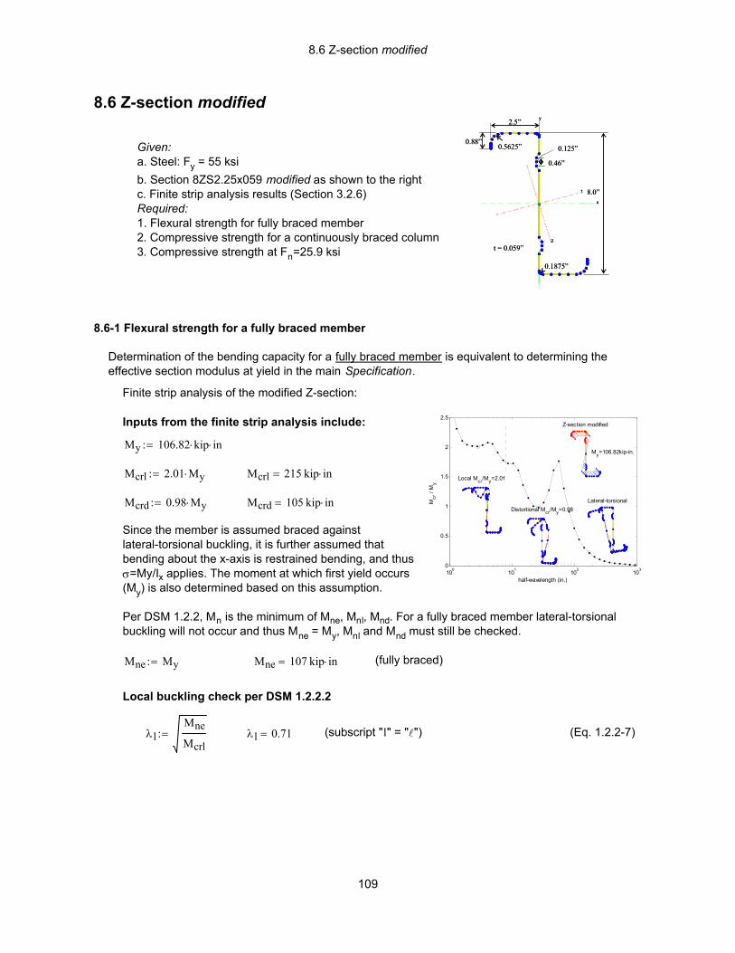
8.6 Z-section modified
(Eq. 1.2.2-7)(subscript "l" = "l")λl 0.71=λlMne
Mcrl:=
Local buckling check per DSM 1.2.2.2
(fully braced)Mne 107 kip in⋅=Mne My:=
Per DSM 1.2.2, Mn is the minimum of Mne, Mnl, Mnd. For a fully braced member lateral-torsional buckling will not occur and thus Mne = My, Mnl and Mnd must still be checked.
Since the member is assumed braced against lateral-torsional buckling, it is further assumed that bending about the x-axis is restrained bending, and thus σ=My/Ix applies. The moment at which first yield occurs (My) is also determined based on this assumption.
Mcrd 105 kip in⋅=Mcrd 0.98 My⋅:=
Mcrl 215 kip in⋅=Mcrl 2.01 My⋅:=
My 106.82 kip⋅ in⋅:=
Inputs from the finite strip analysis include:
100 101 102 1030
0.5
1
1.5
2
2.5
half-wavelength (in.)
Mcr
/ M
y Z-section modified
My=106.82kip-in.
Local Mcr/My=2.01
Distortional Mcr/My=0.98Lateral-torsional
Finite strip analysis of the modified Z-section:
Determination of the bending capacity for a fully braced member is equivalent to determining the effective section modulus at yield in the main Specification.
8.6-1 Flexural strength for a fully braced member
Given: a. Steel: Fy = 55 ksib. Section 8ZS2.25x059 modified as shown to the rightc. Finite strip analysis results (Section 3.2.6)Required:1. Flexural strength for fully braced member2. Compressive strength for a continuously braced column3. Compressive strength at Fn=25.9 ksi
x
y
1
2
8.0”
2.5”
t = 0.059”
0.88”0.5625”
0.1875”
0.46”
0.125”
x
y
1
2
8.0”
2.5”
t = 0.059”
0.88”0.5625”
0.1875”
0.46”
0.125”
8.6 Z-section modified
109
8.6 Z-section modified
Mn
Ωb41 kip in⋅=Ωb 2.0:=ASD:
φb Mn⋅ 66 kip in⋅=φb 0.8:=LRFD:
The geometry of this cross-section is not "pre-qualified" (due to the web stiffeners) and thus the lower φ and higher Ω of the rational analysis clause, main Specification A1.1(b), are used.
Mn 83 kip in⋅=Mn min Mne Mnl Mnd( )( ):=
Predicted flexural strength per DSM 1.3
Distortional buckling readily controls the strength of this cross-section. The modified lip stiffener (from the original 8ZS2.25x059) increases the predicted nominal strength from 76 to 83 kip-in., or 9%.
Mnd 83 kip in⋅=
(Eq. 1.2.2-8)(Eq. 1.2.2-9)
Mnd My λd 0.673≤if
1 0.22Mcrd
My
0.5
⋅−
Mcrd
My
0.5
My⋅
λd 0.673>if
:=
(Eq. 1.2.2-10)λd 1.01=λdMy
Mcrd:=
Distortional buckling check per DSM 1.2.2.3
The local buckling nominal strength is near the yield moment. While local buckling does not control the strength of this cross-section in the fully braced condition (distortional buckling does, see below) for discrete bracing at longer unbraced lengths local buckling in interaction with global buckling will control the strength. Thus, the primary benefit of this cross-section will be to provide higher capacities at longer unbraced length's since little to no reduction will occur due to local buckling. See Chapter 4 for further results.
Mnl 107 kip in⋅=
(Eq. 1.2.2-5)(Eq. 1.2.2-6)
Mnl Mne λl 0.776≤if
1 0.15Mcrl
Mne
0.4
⋅−
Mcrl
Mne
0.4
Mne⋅
λl 0.776>if
:=
local buckling check per DSM 1.2.2.2 (continued)
(Continued) 8.6-1 Flexural strength for a fully braced member
110

8.6 Z-section modified
Pnl 24.63 kip=
Distortional buckling check per DSM 1.2.1.3
λdPy
Pcrd:= λd 1.74= (Eq. 1.2.1-10)
Pnd Py λd 0.561≤if
1 0.25Pcrd
Py
0.6
⋅−
Pcrd
Py
0.6
Py⋅
λd 0.561>if
:= (Eq. 1.2.1-8)(Eq. 1.2.1-9)
though Pcrd is greater than Pcrl, Pnd still controls the strength, reflecting the reduced post-buckling reserve in distortional buckling failures. Pnd 20.5 kip=
Predicted compressive strength per DSM 1.2
Pn min Pne Pnl Pnd( )( ):= Pn 20.5 kip=
The geometry of this section falls outside the "pre-qualified" columns of DSM 1.1.1.1 and thus the lower φ and higher Ω of main Specification A1.1(b) are used.
LRFD: φc 0.8:= φc Pn⋅ 16.4 kip=
ASD: Ωc 2.00:=Pn
Ωc10.2 kip=
8.6-2 Compressive strength for a continuously braced column
Finite strip analysis of the modified Z-section:
100 101 102 1030
0.1
0.2
0.3
0.4
0.5
half-wavelength (in.)
Pcr
/ P
y
Z-section modified
Py=45.64kips
Local Pcr/Py=0.27 Distortional Pcr/Py=0.33
Flexural
Inputs from the finite strip analysis include:Py 45.64 kip⋅:=
Pcrl 0.27 Py⋅:= Pcrl 12.3 kip=
Pcrd 0.33 Py⋅:= Pcrd 15.1 kip=
Per DSM 1.2.1, Pn is the minimum of Pne, Pnl, Pnd. If a column is continuously braced then global buckling Pne is restricted and the squash load will develop if the cross-section is compact.
Pne Py:= Pne 45.64 kip=
Local buckling check per DSM 1.2.1.2
λlPne
Pcrl:= λl 1.92= (subscript "l" = "l") (Eq. 1.2.1-7)
Pnl Pne λl 0.776≤if
1 0.15Pcrl
Pne
0.4
⋅−
Pcrl
Pne
0.4
Pne⋅
λl 0.776>if
:= (Eq. 1.2.1-5)(Eq. 1.2.1-6)
111
8.6 Z-section modified
λdPy
Pcrd:= λd 1.74= (Eq. 1.2.1-10)
Pnd Py λd 0.561≤if
1 0.25Pcrd
Py
0.6
⋅−
Pcrd
Py
0.6
Py⋅
λd 0.561>if
:= (Eq. 1.2.1-8)(Eq. 1.2.1-9)
Pnd 20.5 kip= (note, the distortional buckling prediction is the same as Example 8.6-2, but now no longer controls the predicted strength)
Predicted compressive strength per DSM 1.2
Pn min Pne Pnl Pnd( )( ):= Pn 15.1 kip=
The geometry of this section falls outside the "pre-qualified" columns of DSM 1.1.1.1 and the lower φ and higher Ω of main Specification A1.1(b) are used.
LRFD: φc 0.80:= φc Pn⋅ 12.11 kip= (note, the modified cross-section provides greater strength than the unmodified Z-section of Example 8.5-4)ASD: Ωc 2.00:=
Pn
Ωc7.6 kip=
Note, see Example 8.5-4 for additional discussion on the torsional-flexural compressive strength of a cross-section with decking or sheathing attached to one flange.
8.6-3 Compressive strength at Fn=25.9 ksi
As discussed in Example 8.5-4, AISI (2002) Example III-6 considers the compressive strength of a Z attached to deck or sheathing. Two failure modes are considered, the first of which is restrained flexural buckling about a horizontal axis through the centroid. For the 8ZS2.25x059 the inelastic buckling stress in this mode, Fn, is 25.9 ksi. In the main Specification effective area (Ae) calculations for columns are performed at the stress that the long column can maintain, this stress known as F n is calculated per Eq. C4-2 or C4-3. A similar procedure is perfomed in the Direct Strength Method where the local buckling slenderness and strength equations (DSM Eq.'s 1.2.1-7, and 1.2.1-5,6) are calculated at the strength a long column can maintain, i.e., Pne=AgFn.
for this example, Fn is assumed at 25.9 ksi, therefore... (note Ag 0.83 in2= )
Pne Ag 25.9⋅ ksi⋅:= Pne 21.49 kip=
Local buckling check per DSM 1.2.1.2
(compare with λl of 1.9 for the samecolumn with continuous bracing, see 3.2.5-2)
λlPne
Pcrl:= λl 1.32= (Eq. 1.2.1-7)
Pnl Pne λl 0.776≤if
1 0.15Pcrl
Pne
0.4
⋅−
Pcrl
Pne
0.4
Pne⋅
λl 0.776>if
:= (Eq. 1.2.1-5)(Eq. 1.2.1-6)
Pnl 15.1 kip= (down from 24.6 kips for a column with continuous bracing)
Distortional buckling check per DSM 1.2.1.3
112

8.7 Equal leg angle with lips
Mn
Ωb8 kip in⋅=Ωb 2.0:=ASD: φb Mn⋅ 13 kip in⋅=φb 0.8:=LRFD:
The geometry of this section falls outside the "pre-qualified" beams and the lower φ and higher Ω of the main Specification (Section A1.1b) must be used.
Mn 17 kip in⋅=Mn min Mne Mnl Mnd( )( ):=
Predicted flexural strength per DSM 1.3
The distortional buckling check depends on the unbraced length. In the FSM analysis the largest unbraced length at which distortional buckling is observed is about 20 in. M crd/MY is about 0.6 at this length. Thus, this value could be conservatively used for distortional buckling for any length longer than 20 in. However, if the member is braced against LTB, in this example it is assumed the member is braced against distortional buckling as well. Therefore, for a fully braced member it is expected that no reduction occurs due to distortional buckling and M nd=My.
Distortional buckling check per DSM 1.2.2.3
Mnl My:=per Section 2.2 of this Guide Mcrl>1.66My, therefore
Local buckling check per DSM 1.2.2.2
(fully braced)Mne 17 kip in⋅=Mne My:=
Per DSM 1.2.2, Mn is the minimum of Mne, Mnl, Mnd. For a fully braced member lateral-torsional buckling will not occur and thus Mne = MY, Mnl and Mnd must still be checked.
Mcrl 28 kip in⋅=Mcrl 1.69 My⋅:=
My 16.85 kip⋅ in⋅:=
Inputs from the finite strip analysis include:
100 101 102 1030
0.2
0.4
0.6
0.8
1
1.2
1.4
1.6
1.8
2
half-wavelength (in.)
Mcr
/ M
y
Angle with lips (AISI 2002 Ex. I-11)
My=16.85kip-in.Local Mcr/My=1.69
Distortional
Lateral-torsional
Consider finite strip analysis of 4LS4x060 in restrained bending as summarized in Section 3.2.7
Determination of the bending strength for a fully braced member is equivalent to determining the effective section modulus at yield in the main Specification.
8.7-1 Flexural strength for a full braced member
C x
y
1
1
2
2
4.0”
4.0”
0.5”
0.5”
0.1875”
C x
y
1
1
2
2
C x
y
1
1
2
2
4.0”
4.0”
0.5”
0.5”
0.1875”
Given: a. Steel: Fy = 50 ksib. Section 4LS4x0606 as shown to the rightc. Finite strip analysis results (Section 3.2.7)Required:1. Flexural strength about x-asis for a fully braced member2. Flexural strength about minimum principal axis for L=18 in. (AISI 2002 Example III-4)3. Compressive strength for a continuously braced member4. Compressive strength at Fn=14.7 ksi (AISI 2002 Example III-4)5. Compression strength considering eccentricity (AISI 2002 Example III-4)
8.7 Equal leg angle with lips
113

8.7 Equal leg angle with lips
that can be compared with an Fc of 33.47 ksi calculated in AISI (2002) Example III-4.
Local buckling check per DSM 1.2.2.2
Mcrl is significantly greater than 1.66My and therefore no local reduction will occur.
Mnl Mne:=
Distortional buckling check per DSM 1.2.2.3
Mcrd is not relevant to this cross-section as it is not separate from the global (lateral-torsional) mode, set Mnd to My in this case.
Mnd My:=
Predicted flexural strength per DSM 1.3
Mn min Mne Mnl Mnd( )( ):= Mn 8.4 kip in⋅=
The geometry of this section falls outside the "pre-qualified" beams and the lower φ and higher Ω of the main Specification (Section A1.1b) must be used.
LRFD: φb 0.8:= φb Mn⋅ 6.72 kip in⋅= ASD: Ωb 2.0:=Mn
Ωb4.2 kip in⋅=
8.7-2 Flexural strength about minimum principal axis for L=18 in., (AISI 2002 Example III-4)
Example III-4 of AISI (2002) consider the compressive strength of this cross-section over an 18 in. length, however, per Sections C4(b) and C5.2 of the main Specification, the effect of an eccentricity of PL/1000 about the minor axis must be considered.
This example provides the bending strength about the minimum principal axis at L=18 in.
100 101 1020
1
2
3
4
5
6
half-wavelength (in.)
Mcr
/ M
y
Angle with lips (AISI 2002 Ex. I-11)
My=12.66kip-in.Local Mcr/My=4.93
Torsional Mcr/My=0.69
Inputs from the finite strip analysis include:
My 12.66 kip⋅ in⋅:=
Mcrl 4.93 My⋅:= Mcrl 62 kip in⋅=
Mcre 0.69 My⋅:= at 18 in. Mcre 8.74 kip in⋅=
Lateral-torsional buckling check per DSM 1.2.2.1
Mne Mcre Mcre 0.56 My⋅<if
109
My⋅ 110 My⋅
36 Mcre⋅−
⋅
2.78 My⋅ Mcre≥ 0.56 My⋅≥if
My Mcre 2.78 My⋅>if
:= (Eq. 1.2.2-1)
(Eq. 1.2.2-2)
(Eq. 1.2.2-3)
Mne 8.4 kip in⋅= Mne
Sg2233.19 ksi=
114
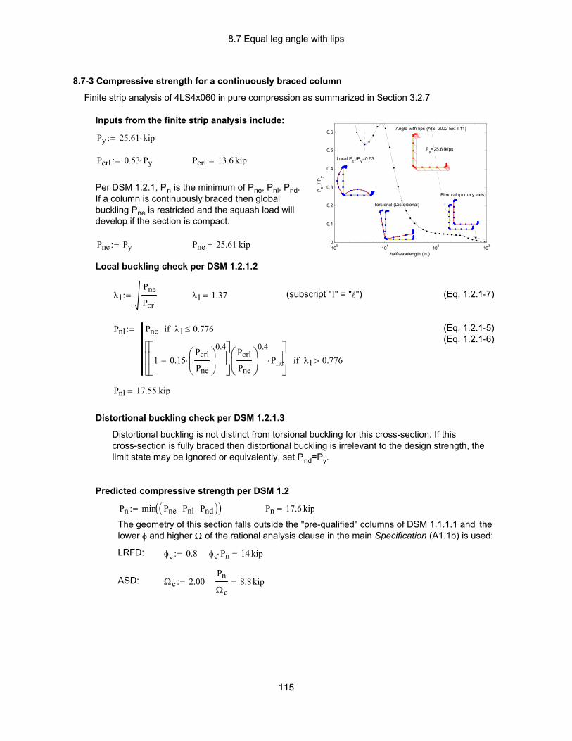
8.7 Equal leg angle with lips
Pn
Ωc8.8 kip=Ωc 2.00:=ASD:
φc Pn⋅ 14 kip=φc 0.8:=LRFD:
The geometry of this section falls outside the "pre-qualified" columns of DSM 1.1.1.1 and the lower φ and higher Ω of the rational analysis clause in the main Specification (A1.1b) is used:
Pn 17.6 kip=Pn min Pne Pnl Pnd( )( ):=
Predicted compressive strength per DSM 1.2
Distortional buckling is not distinct from torsional buckling for this cross-section. If this cross-section is fully braced then distortional buckling is irrelevant to the design strength, the limit state may be ignored or equivalently, set Pnd=Py.
Distortional buckling check per DSM 1.2.1.3
Pnl 17.55 kip=
(Eq. 1.2.1-5)(Eq. 1.2.1-6)
Pnl Pne λl 0.776≤if
1 0.15Pcrl
Pne
0.4
⋅−
Pcrl
Pne
0.4
Pne⋅
λl 0.776>if
:=
(Eq. 1.2.1-7)(subscript "l" = "l")λl 1.37=λlPne
Pcrl:=
Local buckling check per DSM 1.2.1.2
Pne 25.61 kip=Pne Py:=
Per DSM 1.2.1, Pn is the minimum of Pne, Pnl, Pnd. If a column is continuously braced then global buckling Pne is restricted and the squash load will develop if the section is compact.
Pcrl 13.6 kip=Pcrl 0.53 Py⋅:=
Py 25.61 kip⋅:=
Inputs from the finite strip analysis include:
100 101 102 1030
0.1
0.2
0.3
0.4
0.5
0.6
half-wavelength (in.)
Pcr
/ P
y
Angle with lips (AISI 2002 Ex. I-11)
Py=25.61kips
Local Pcr/Py=0.53
Torsional (Distortional)
Flexural (primary axis)
Finite strip analysis of 4LS4x060 in pure compression as summarized in Section 3.2.7
8.7-3 Compressive strength for a continuously braced column
115
8.7 Equal leg angle with lips
Pne 7.53 kip=
Local buckling check per DSM 1.2.1.2
(compare with λl of 2.9 for the same column with continuous bracing, see Example 8.7-3)
λlPne
Pcrl:= λl 0.74= (Eq. 1.2.1-7)
since λl<0.776 per Eq. 1.2.1-5 Pnl Pne:= (down from 17.55 kips for continuous bracing)
Distortional buckling check per DSM 1.2.1.3
Distortional buckling is not distinct from torsional buckling in this section. The limit state may beignored or equivalently, set Pnd=Py.
Predicted compressive strength per DSM 1.2
Pn min Pne Pnl Pnd( )( ):= Pn 7.53 kip=
The geometry of this section falls outside the "pre-qualified" columns of DSM 1.1.1.1 and the lower φ and higher Ω of the rational analysis clause in the main Specification (A1.1b) is used:
LRFD: φc 0.8:= φc Pn⋅ 6.02 kip= ASD: Ωc 2.00:=Pn
Ωc3.76 kip=
8.7-4 Compressive strength at Fn=14.7 ksi (AISI 2002 Example III-4)
AISI (2002) Example III-4 considers this 4LS4x059 cross-section as an 18 in. long column. The cross-section is concentrically loaded in compression and KLx=KLY=KLt=18 in. AISI (2002) Example III-4 provides the lengthy Specification formulas (C4) for determining the global buckling strength of this column, while AISI (2002) Example I-4 provides the effective area. This example provides the concentric compressive strength using DSM. Finite strip analysis of 4LS4x059 in pure compression is the same as used in Example 8.7-3 with Py, Pcrl, etc., from Example 8.7-3 (Section 3.2.7), the following is obtained:
Pcre 0.31 Py⋅:= at 18 in. Pcre 7.94 kip=Pcre
Ag15.5 ksi= compare with 16.7 ksi by the formula
given in Example III-4 of AISI (2002)
Flexural, Torsional, or Torsional-Flexural check per DSM 1.2.1.1
λcPy
Pcre:= λc 1.8= (in the elastic buckling regime) (Eq. 1.2.1-1)
Pne 0.658λ c
2
Py⋅ λc 1.5≤if
.877
λc2
Py⋅ λc 1.5>if
:= (Eq. 1.2.1-2)
(Eq. 1.2.1-3)
Pne 6.96 kip= or as stress:Pne
Ag13.59 ksi= which itself is Fn in the main Spec.
(14.7 ksi in example III-4 of AISI 2002).In the main Specification effective area (Ae) calculations for columns are performed at the stress that the long column can maintain, this stress known as Fn is calculated per Eq. C4-2 or C4-3. A similar procedure is perfomed in the Direct Strength Method where the local buckling slenderness and strength equations (1.2.1-7, and 1.2.1-5,6) are calcualted at the strength a long column can maintain, i.e., Pne=AgFn. Per DSM 1.2.1, Pn is the minimum of Pne, Pnl, Pnd.
for comparison to AISI (2002) Examples I-11 and III-4 assume Fn is 14.7 ksi and continue with the Direct Strength Method. (Alternatively Pne calculated above could be used.)
Pne Ag 14.7⋅ ksi⋅:=
116
8.7 Equal leg angle with lips
Interaction equations
assume Pu
φc Pn⋅is > 0.15, therefore use Equations C5.2.2-1 and C5.2.2-2 and find P u
Pu
0.8 7.53⋅
1.0 0.0180⋅ Pu⋅
0.8 8.4⋅ 1Pu
357−
⋅
+ 1≤Pu
φc Pn⋅
Cm Mu⋅
φb Mn⋅ α2⋅+ 1≤ (Eq. C5.2.2-1)
Pu 5.93≤
Pu
φc Pno⋅
Mu
φb Mn⋅+ 1≤
Pu
0.8 17.6⋅
0.0180 Pu⋅
0.8 8.4⋅+ 1≤ (Eq. C5.2.2-2)
Pu 13.57≤
per main Specification C5.2.2-1 the required strength (LRFD) Pu, is 5.93 kip⋅
Check that Pu
φc Pn⋅is greater than 0.15, 5.93
0.8 7.53⋅0.98= OK
see AISI (2002) Design Manual Example III-4 for ASD format.
8.7-5 Compressive strength considering eccentricity (AISI 2002 Example III-4)
Continuing from Example 8.7-4 above, this example considers the compressive capacity of this same cross-section with the effect of an eccentricity of PL/1000 about the minor axis. This is a continuation of AISI (2002) Design Manual Example III-4.
Compression: the compressive strength of this cross-section as determined in Example 8.7-4.
φc 0.8= Pn 7.53 kip=
for the C5.2.2-2 interaction equation the fully braced compressive strength is needed, per 8.7-3
Pno 17.6 kip=
Bending: the flexural strength of this section as determined in Example 8.7-2 above
φb 0.8= Mn 8.4 kip in⋅=
Factors to account for approximate 2nd order analysis
MuxP L⋅1000
:=P First order moment demand for L=18 in. is 0.0180P
Cm 1.0:= The member is pinned, accidental eccentricity places a constant moment demand, 2nd order moments and primary moments are at the same location, and C m should be 1.0.
α2 is the moment amplification term for minor principal axis bending moment. The demand axial load P is to be solved for in this case. The elastic buckling load about the minor principal axis can be determined by Equation C5.2.1-7 in the main Specification, or taken from finite strip analysis.
α2 1Pu
PE2−:=
PE2
PE2 357 kip⋅:= from Eq. C5.2.1-7 as used in AISI (2002) Example III-4
117
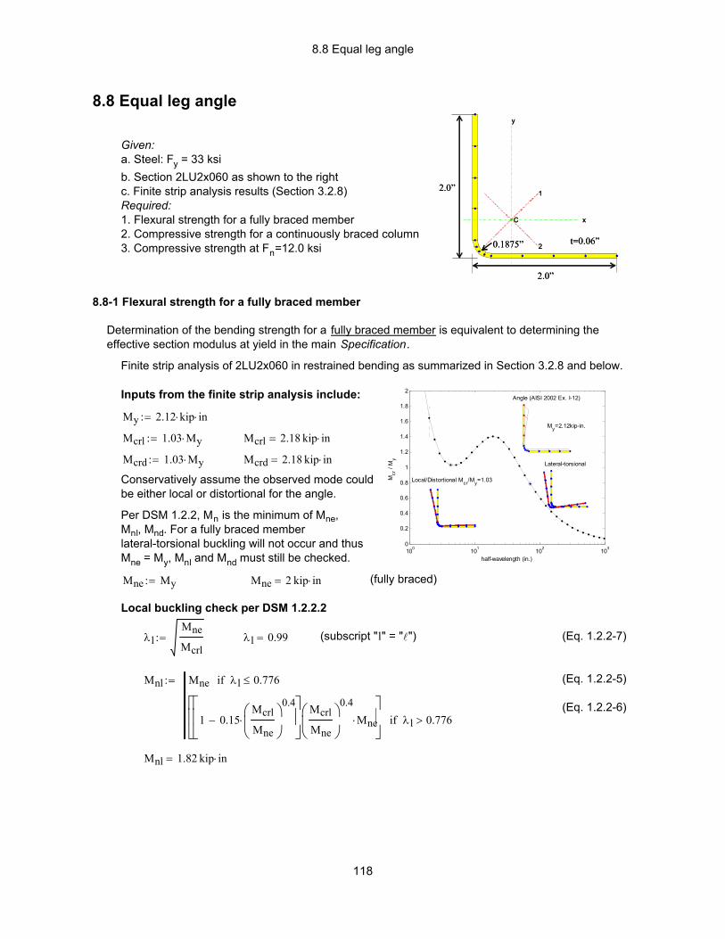
8.8 Equal leg angle
Mnl 1.82 kip in⋅=
(Eq. 1.2.2-5)
(Eq. 1.2.2-6)
Mnl Mne λl 0.776≤if
1 0.15Mcrl
Mne
0.4
⋅−
Mcrl
Mne
0.4
Mne⋅
λl 0.776>if
:=
(Eq. 1.2.2-7)(subscript "l" = "l")λl 0.99=λlMne
Mcrl:=
Local buckling check per DSM 1.2.2.2
(fully braced)Mne 2 kip in⋅=Mne My:=
Per DSM 1.2.2, Mn is the minimum of Mne, Mnl, Mnd. For a fully braced member lateral-torsional buckling will not occur and thus Mne = My, Mnl and Mnd must still be checked.
Conservatively assume the observed mode couldbe either local or distortional for the angle.
Mcrd 2.18 kip in⋅=Mcrd 1.03 My⋅:=
Mcrl 2.18 kip in⋅=Mcrl 1.03 My⋅:=
My 2.12 kip⋅ in⋅:=
Inputs from the finite strip analysis include:
100 101 102 1030
0.2
0.4
0.6
0.8
1
1.2
1.4
1.6
1.8
2
half-wavelength (in.)
Mcr
/ M
y Angle (AISI 2002 Ex. I-12)
My=2.12kip-in.
Local/Distortional Mcr/My=1.03
Lateral-torsional
Finite strip analysis of 2LU2x060 in restrained bending as summarized in Section 3.2.8 and below.
Determination of the bending strength for a fully braced member is equivalent to determining the effective section modulus at yield in the main Specification.
8.8-1 Flexural strength for a fully braced member
Given: a. Steel: Fy = 33 ksib. Section 2LU2x060 as shown to the rightc. Finite strip analysis results (Section 3.2.8)Required:1. Flexural strength for a fully braced member2. Compressive strength for a continuously braced column3. Compressive strength at Fn=12.0 ksi
C x
y
1
2
2.0”
2.0”
0.1875” t=0.06”
C x
y
1
2
2.0”
2.0”
0.1875” t=0.06”
8.8 Equal leg angle
118

8.8 Equal leg angle
Mn
Ωb0.84 kip in⋅=Ωb 2.0:=ASD: φb Mn⋅ 1.34 kip in⋅=φb 0.8:=LRFD:
The geometry of this section falls outside the "pre-qualified" beams and the lower φ and higher Ω of the main Specification (Section A1.1b) must be used.
Mn 2 kip in⋅=Mn min Mne Mnl Mnd( )( ):=
Predicted flexural strength per DSM 1.3
Distortional buckling controls the predicted strength, which given M crl=Mcrd will always be the case when LTB is assumed fully braced (Mne=My), if LTB reduces the bending strength slightly Mne<MY, then Mnl will quickly control the strength, for more on this topic see Chapter 4 of this Guide.
Mnd 1.67 kip in⋅=
(Eq. 1.2.2-8)
(Eq. 1.2.2-9)
Mnd My λd 0.673≤if
1 0.22Mcrd
My
0.5
⋅−
Mcrd
My
0.5
My⋅
λd 0.673>if
:=
(Eq. 1.2.2-10)λd 0.99=λdMy
Mcrd:=
Distortional buckling check per DSM 1.2.2.3
119

8.8 Equal leg angle
Pn
Ωc2.1 kip=Ωc 2.00:=ASD:
φc Pn⋅ 3.4 kip=φc 0.8:=LRFD:
The geometry of this section falls outside the "pre-qualified" columns of DSM 1.1.1.1 and the lower φ and higher Ω of the rational analysis clause in the main Specification (A1.1b) is used:
Pn 4.3 kip=Pn min Pne Pnl Pnd( )( ):=
Predicted compressive strength per DSM 1.2
Distortional buckling is not distinct from torsional buckling in this section. If this section is fully braced then distortional buckling is irrelevant to the design strength, we may ignore the limit state or equivalently, set Pnd=Py.
Distortional buckling check per DSM 1.2.1.3
Pnl 4.27 kip=
(Eq. 1.2.1-5)(Eq. 1.2.1-6)
Pnl Pne λl 0.776≤if
1 0.15Pcrl
Pne
0.4
⋅−
Pcrl
Pne
0.4
Pne⋅
λl 0.776>if
:=
8.8-2 Compressive strength for a continuously braced column
Here the defintion of "continuous" bracing plays an important role in determining how to proceed with the strength calculation. If the bracing restrains torsion and flexure then a specific analysis with the bracing included would be needed to determine what manner of local buckling may still occur. If the bracing restricts flexure only, but allows torsion then the plateau at approximately 0.3PY would be relevant as a local torsional mode is possible. For this example, it is assumed that the bracing removes the long column flexural mode, but not the shorter torsional mode.
Finite strip analysis of 2LS2x060:
100 101 102 1030
0.1
0.2
0.3
0.4
0.5
0.6
0.7
0.8
0.9
half-wavelength (in.)
Pcr
/ P
y
Angle (AISI 2002 Ex. I-12)
Py=7.61kips
Local/Distortional/Torsional
Flexural (primary axis)
Inputs from the finite strip analysis include:
Py 7.61 kip⋅:=
Pcrl 0.3 Py⋅:= Pcrl 2.3 kip=
Per DSM 1.2.1, Pn is the minimum of Pne, Pnl, Pnd. If a column is continuously braced then global buckling Pne is restricted and the squash load will develop if the cross-section is compact.
Pne Py:= Pne 7.61 kip=
Local buckling check per DSM 1.2.1.2
λlPne
Pcrl:= λl 1.83= (subscript "l" = "l") (Eq. 1.2.1-7)
120

8.8 Equal leg angle
Pn
Ωc1.1 kip=Ωc 2.00:=ASD:
φc Pn⋅ 1.77 kip=φc 0.8:=LRFD:
The geometry of this section falls outside the "pre-qualified" columns of DSM 1.1.1.1 and the lower φ and higher Ω of the rational analysis clause in the main Specification (A1.1b) is used:
Pn 2.21 kip=Pn min Pne Pnl Pnd( )( ):=
Predicted compressive strength per DSM 1.2
Distortional buckling is not distinct from torsional buckling in this cross-section. If this cross-section is fully braced then distortional buckling is irrelevant to the design strength, the limit state may beignroed or equivalently, set Pnd=Py.
Distortional buckling check per DSM 1.2.1.3
(down from 4.3 kips for a column with continuous bracing)Pnl 2.21 kip=
(Eq. 1.2.1-5)(Eq. 1.2.1-6)
Pnl Pne λl 0.776≤if
1 0.15Pcrl
Pne
0.4
⋅−
Pcrl
Pne
0.4
Pne⋅
λl 0.776>if
:=
(Eq. 1.2.1-7)λl 1.1=λlPne
Pcrl:=
(compare with λl of 1.8 for the same column with continuous bracing, see Example 8.8-2)
Local buckling check per DSM 1.2.1.2
From the finite strip analysis the long column buckling mode is likely flexure, in which case a local mode dominated by torsion may possibly interact. Conservatively, this interaction is included in the calculation.
Pne 2.77 kip=Pne Ag 12⋅ ksi⋅:=
In the main Specification effective area (Ae) calculations for columns are performed at the stress that the long column can maintain, this stress known as Fn is calculated per Eq. C4-2 or C4-3. A similar procedure is perfomed in the Direct Strength Method where the local buckling slenderness and strength equations (1.2.1-7, and 1.2.1-5,6) are calculated at the strength a long column can maintain, i.e., Pne=AgFn. Per DSM 1.2.1, Pn is the minimum of Pne, Pnl, Pnd.
Finite strip analysis of 2LU2x060 in pure compression is the same as used in Example 8.8-2.
8.8-3 Compression strength at Fn=12.0 ksi
121
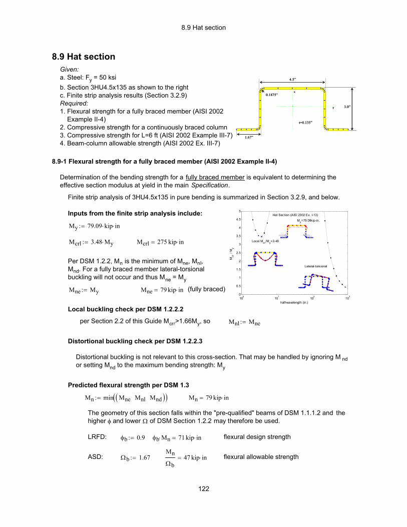
8.9 Hat section
flexural allowable strengthMn
Ωb47 kip in⋅=Ωb 1.67:=ASD:
flexural design strengthφb Mn⋅ 71 kip in⋅=φb 0.9:=LRFD:
The geometry of this section falls within the "pre-qualified" beams of DSM 1.1.1.2 and the higher φ and lower Ω of DSM Section 1.2.2 may therefore be used.
Mn 79 kip in⋅=Mn min Mne Mnl Mnd( )( ):=
Predicted flexural strength per DSM 1.3
Distortional buckling is not relevant to this cross-section. That may be handled by ignoring M nd or setting Mnd to the maximum bending strength: My
Distortional buckling check per DSM 1.2.2.3
Mnl Mne:=
8.9 Hat sectionGiven: a. Steel: Fy = 50 ksib. Section 3HU4.5x135 as shown to the rightc. Finite strip analysis results (Section 3.2.9)Required:1. Flexural strength for a fully braced member (AISI 2002 Example II-4)2. Compressive strength for a continuously braced column3. Compressive strength for L=6 ft (AISI 2002 Example III-7)4. Beam-column allowable strength (AISI 2002 Ex. III-7)
3.0”
4.5”
1.67”
0.1875”
t=0.135”
x
y 3.0”
4.5”
1.67”
0.1875”
t=0.135”
x
y
8.9-1 Flexural strength for a fully braced member (AISI 2002 Example II-4)
Determination of the bending strength for a fully braced member is equivalent to determining the effective section modulus at yield in the main Specification.
Finite strip analysis of 3HU4.5x135 in pure bending is summarized in Section 3.2.9, and below.
100
101
102
103
0
0.5
1
1.5
2
2.5
3
3.5
4
4.5
5
half-wavelength (in.)
Mcr
/ M
y
Hat Section (AISI 2002 Ex. I-13)
My=79.09kip-in.
Local Mcr/My=3.48
Lateral-torsional
Inputs from the finite strip analysis include:
My 79.09 kip⋅ in⋅:=
Mcrl 3.48 My⋅:= Mcrl 275 kip in⋅=
Per DSM 1.2.2, Mn is the minimum of Mne, Mnl, Mnd. For a fully braced member lateral-torsional buckling will not occur and thus Mne = My
Mne My:= Mne 79 kip in⋅= (fully braced)
Local buckling check per DSM 1.2.2.2
per Section 2.2 of this Guide Mcrl>1.66My, so
122
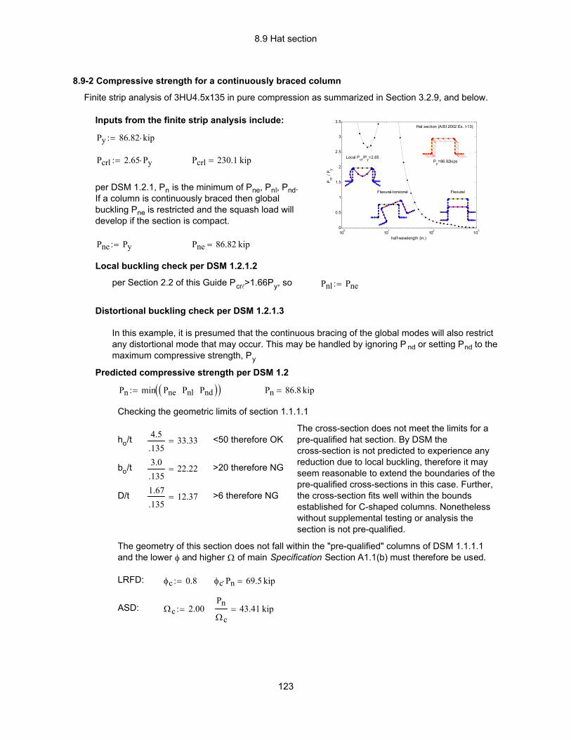
8.9 Hat section
Checking the geometric limits of section 1.1.1.1
The cross-section does not meet the limits for a pre-qualified hat section. By DSM the cross-section is not predicted to experience any reduction due to local buckling, therefore it may seem reasonable to extend the boundaries of the pre-qualified cross-sections in this case. Further, the cross-section fits well within the bounds established for C-shaped columns. Nonetheless without supplemental testing or analysis the section is not pre-qualified.
ho/t 4.5.135
33.33= <50 therefore OK
bo/t 3.0.135
22.22= >20 therefore NG
D/t 1.67.135
12.37= >6 therefore NG
The geometry of this section does not fall within the "pre-qualified" columns of DSM 1.1.1.1 and the lower φ and higher Ω of main Specification Section A1.1(b) must therefore be used.
LRFD: φc 0.8:= φc Pn⋅ 69.5 kip=
ASD: Ωc 2.00:=Pn
Ωc43.41 kip=
8.9-2 Compressive strength for a continuously braced column
Finite strip analysis of 3HU4.5x135 in pure compression as summarized in Section 3.2.9, and below.
100 101 102 1030
0.5
1
1.5
2
2.5
3
3.5
half-wavelength (in.)
Pcr
/ P y
Hat section (AISI 2002 Ex. I-13)
Py=86.82kipsLocal Pcr/Py=2.65
Flexural-torsional Flexural
Inputs from the finite strip analysis include:
Py 86.82 kip⋅:=
Pcrl 2.65 Py⋅:= Pcrl 230.1 kip=
per DSM 1.2.1, Pn is the minimum of Pne, Pnl, Pnd. If a column is continuously braced then global buckling Pne is restricted and the squash load will develop if the section is compact.
Pne Py:= Pne 86.82 kip=
Local buckling check per DSM 1.2.1.2
per Section 2.2 of this Guide Pcrl>1.66Py, so Pnl Pne:=
Distortional buckling check per DSM 1.2.1.3
In this example, it is presumed that the continuous bracing of the global modes will also restrict any distortional mode that may occur. This may be handled by ignoring P nd or setting Pnd to the maximum compressive strength, Py
Predicted compressive strength per DSM 1.2
Pn min Pne Pnl Pnd( )( ):= Pn 86.8 kip=
123
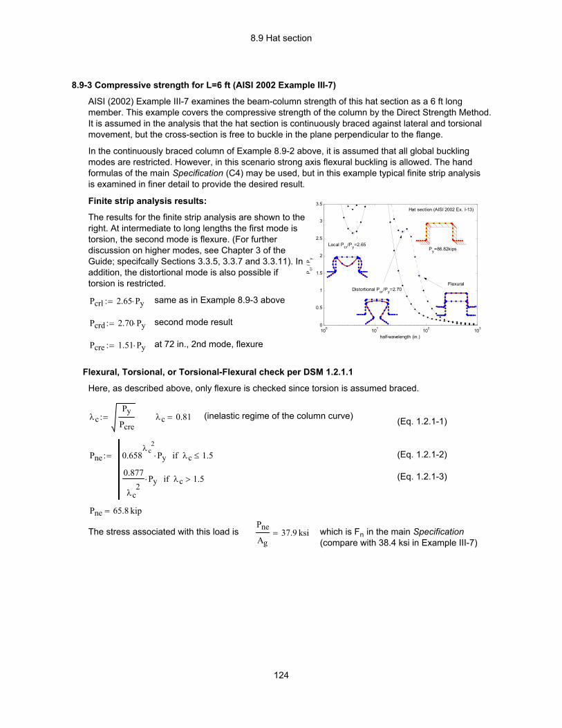
8.9 Hat section
which is Fn in the main Specification (compare with 38.4 ksi in Example III-7)
Pne
Ag37.9 ksi=The stress associated with this load is
Pne 65.8 kip=
(Eq. 1.2.1-3)
(Eq. 1.2.1-2)Pne 0.658λ c
2
Py⋅ λc 1.5≤if
0.877
λc2
Py⋅ λc 1.5>if
:=
(Eq. 1.2.1-1)(inelastic regime of the column curve)λc 0.81=λcPy
Pcre:=
Here, as described above, only flexure is checked since torsion is assumed braced.
Flexural, Torsional, or Torsional-Flexural check per DSM 1.2.1.1
at 72 in., 2nd mode, flexurePcre 1.51 Py⋅:=
second mode resultPcrd 2.70 Py⋅:=
same as in Example 8.9-3 abovePcrl 2.65 Py⋅:=
The results for the finite strip analysis are shown to the right. At intermediate to long lengths the first mode is torsion, the second mode is flexure. (For further discussion on higher modes, see Chapter 3 of the Guide; specifcally Sections 3.3.5, 3.3.7 and 3.3.11). In addition, the distortional mode is also possible if torsion is restricted.
Finite strip analysis results:
100 101 102 1030
0.5
1
1.5
2
2.5
3
3.5
half-wavelength (in.)
Pcr
/ P
y
Hat section (AISI 2002 Ex. I-13)
Py=86.82kipsLocal Pcr/Py=2.65
Distortional Pcr/Py=2.70Flexural
In the continuously braced column of Example 8.9-2 above, it is assumed that all global buckling modes are restricted. However, in this scenario strong axis flexural buckling is allowed. The hand formulas of the main Specification (C4) may be used, but in this example typical finite strip analysis is examined in finer detail to provide the desired result.
AISI (2002) Example III-7 examines the beam-column strength of this hat section as a 6 ft long member. This example covers the compressive strength of the column by the Direct Strength Method. It is assumed in the analysis that the hat section is continuously braced against lateral and torsional movement, but the cross-section is free to buckle in the plane perpendicular to the flange.
8.9-3 Compressive strength for L=6 ft (AISI 2002 Example III-7)
124

8.9 Hat section
Pn
Ωc32.9 kip=Ωc 2.00:=ASD:
φc Pn⋅ 52.6 kip=φc 0.8:=LRFD:
The geometry of this section does not fall within the "pre-qualified" columns of DSM 1.1.1.1 and the lower φ and higher Ω of main Specification Section A1.1(b) must therefore be used.
Pn 65.8 kip=Pn min Pne Pnl Pnd( )( ):=
Predicted compressive strength per DSM 1.2
(at this length this does not control; however Pnd is slightly lower than PY so at a short enough length Pnd will control the strength)
Pnd 86.1 kip=
(Eq. 1.2.1-8)
(Eq. 1.2.1-9)
Pnd Py λd 0.561≤if
1 0.25Pcrd
Py
0.6
⋅−
Pcrd
Py
0.6
Py⋅
λd 0.561>if
:=
(Eq. 1.2.1-10)λd 0.61=λdPy
Pcrd:=
Distortional buckling check per DSM 1.2.1.3
Pnl Pne:=per 2.2 of this guide Pcrl>1.66Py, so Pnl=Pne
Local buckling check per DSM 1.2.1.2
(continued) 8.9-3 Compressive strength for L=6 ft (AISI 2002 Example III-7)
125
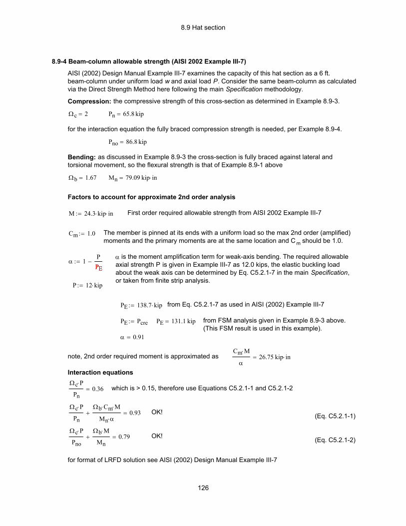
8.9 Hat section
PE 138.7 kip⋅:= from Eq. C5.2.1-7 as used in AISI (2002) Example III-7
PE Pcre:= PE 131.1 kip= from FSM analysis given in Example 8.9-3 above. (This FSM result is used in this example).
α 0.91=
note, 2nd order required moment is approximated asCm M⋅
α26.75 kip in⋅=
Interaction equationsΩc P⋅
Pn0.36= which is > 0.15, therefore use Equations C5.2.1-1 and C5.2.1-2
Ωc P⋅
Pn
Ωb Cm⋅ M⋅
Mn α⋅+ 0.93= OK! (Eq. C5.2.1-1)
Ωc P⋅
Pno
Ωb M⋅
Mn+ 0.79= OK! (Eq. C5.2.1-2)
for format of LRFD solution see AISI (2002) Design Manual Example III-7
8.9-4 Beam-column allowable strength (AISI 2002 Example III-7)
AISI (2002) Design Manual Example III-7 examines the capacity of this hat section as a 6 ft. beam-column under uniform load w and axial load P. Consider the same beam-column as calculated via the Direct Strength Method here following the main Specification methodology.
Compression: the compressive strength of this cross-section as determined in Example 8.9-3.
Ωc 2= Pn 65.8 kip=
for the interaction equation the fully braced compression strength is needed, per Example 8.9-4.
Pno 86.8 kip=
Bending: as discussed in Example 8.9-3 the cross-section is fully braced against lateral and torsional movement, so the flexural strength is that of Example 8.9-1 above
Ωb 1.67= Mn 79.09 kip in⋅=
Factors to account for approximate 2nd order analysis
M 24.3 kip⋅ in⋅:= First order required allowable strength from AISI 2002 Example III-7
Cm 1.0:= The member is pinned at its ends with a uniform load so the max 2nd order (amplified) moments and the primary moments are at the same location and C m should be 1.0.
α is the moment amplification term for weak-axis bending. The required allowable axial strength P is given in Example III-7 as 12.0 kips, the elastic buckling load about the weak axis can be determined by Eq. C5.2.1-7 in the main Specification, or taken from finite strip analysis.
α 1PPE
−:=PE
P 12 kip⋅:=
126
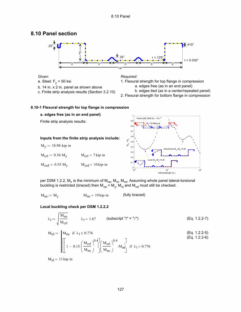
8.10 Panel
Mnl 11 kip in⋅=
(Eq. 1.2.2-5)(Eq. 1.2.2-6)
Mnl Mne λl 0.776≤if
1 0.15Mcrl
Mne
0.4
⋅−
Mcrl
Mne
0.4
Mne⋅
λl 0.776>if
:=
(Eq. 1.2.2-7)(subscript "l" = "l")λl 1.67=λlMne
Mcrl:=
Local buckling check per DSM 1.2.2.2
(fully braced)Mne 19 kip in⋅=Mne My:=
per DSM 1.2.2, Mn is the minimum of Mne, Mnl, Mnd. Assuming whole panel lateral-torsional buckling is restricted (braced) then Mne = My, Mnl and Mnd must still be checked.
Mcrd 10 kip in⋅=Mcrd 0.55 My⋅:=
Mcrl 7 kip in⋅=Mcrl 0.36 My⋅:=
My 18.98 kip⋅ in⋅:=
Inputs from the finite strip analysis include:
Finite strip analysis results:
a. edges free (as in an end panel)
100 101 1020
0.1
0.2
0.3
0.4
0.5
0.6
0.7
0.8
0.9
1
half-wavelength (in.)
Mcr
/ M
y
Panel (AISI 2002 Ex. I-14)
My=18.98kip-in.
Local Mcr/My=0.36
Distortional Mcr/My=0.55
8.10-1 Flexural strength for top flange in compression
Required:1. Flexural strength for top flange in compression
a. edges free (as in an end panel)b. edges tied (as in a center/repeated panel)
2. Flexural strength for bottom flange in compression
Given: a. Steel: Fy = 50 ksib. 14 in. x 2 in. panel as shown abovec. Finite strip analysis results (Section 3.2.10)
3” 3” 3” 3” 2”14”
2”
.25” .415”
r =.125”.35”t = 0.030”
3” 3” 3” 3” 2”14”
2”
.25” .415”
r =.125”.35”t = 0.030”
8.10 Panel section
127
8.10 Panel
Mn
Ωb5.7 kip in⋅=Ωb 2.0:=ASD:
φb Mn⋅ 9.1 kip in⋅=φb 0.8:=LRFD:
The geometry of this section falls outside the "pre-qualified" beams of DSM 1.1.1.2 and the lower φ and higher Ω of main Specification Section A1.1b are therefore used.
Mn 11.4 kip in⋅=Mn min Mne Mnl Mnd( )( ):=
Predicted flexural strength per DSM 1.3
Mnd 12 kip in⋅=
(Eq. 1.2.2-8)(Eq. 1.2.2-9)
Mnd My λd 0.673≤if
1 0.22Mcrd
My
0.5
⋅−
Mcrd
My
0.5
My⋅
λd 0.673>if
:=
(Eq. 1.2.2-10)λd 1.35=λdMy
Mcrd:=
Distortional buckling check per DSM 1.2.2.3
(continued) 8.10-1 Flexural strength for top flange in compression
128
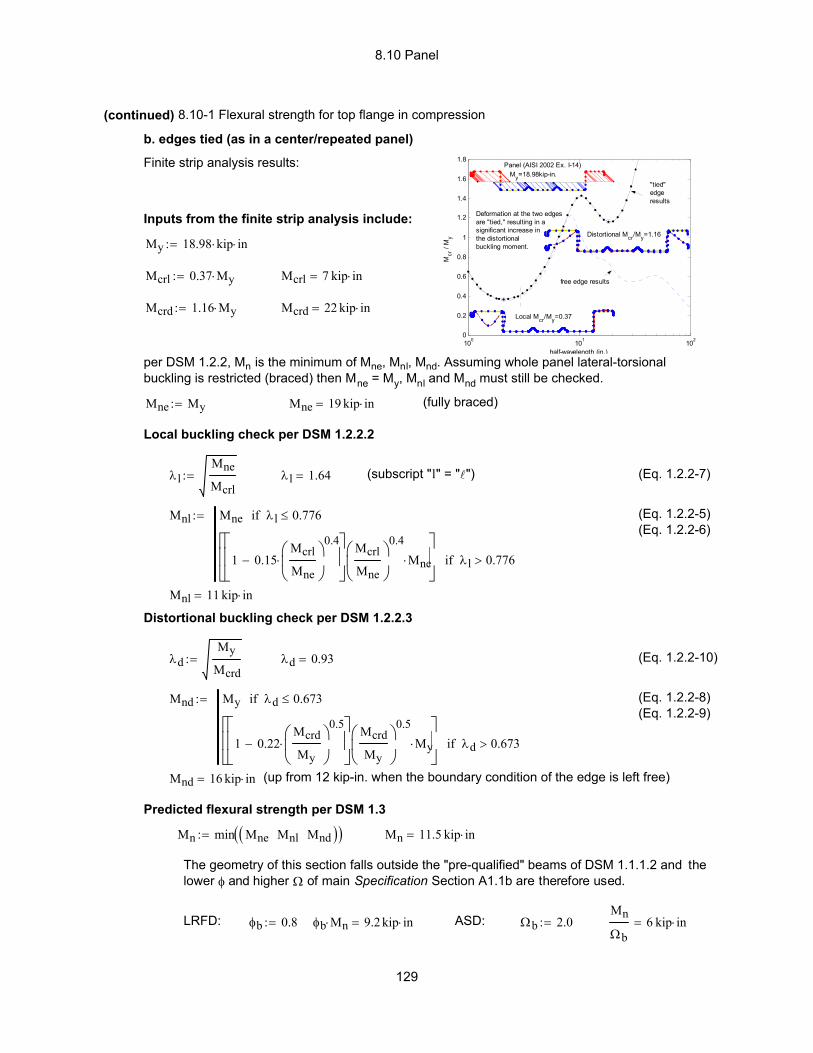
8.10 Panel
(Eq. 1.2.2-5)(Eq. 1.2.2-6)
Mnl 11 kip in⋅=
Distortional buckling check per DSM 1.2.2.3
λdMy
Mcrd:= λd 0.93= (Eq. 1.2.2-10)
Mnd My λd 0.673≤if
1 0.22Mcrd
My
0.5
⋅−
Mcrd
My
0.5
My⋅
λd 0.673>if
:= (Eq. 1.2.2-8)(Eq. 1.2.2-9)
Mnd 16 kip in⋅= (up from 12 kip-in. when the boundary condition of the edge is left free)
Predicted flexural strength per DSM 1.3
Mn min Mne Mnl Mnd( )( ):= Mn 11.5 kip in⋅=
The geometry of this section falls outside the "pre-qualified" beams of DSM 1.1.1.2 and the lower φ and higher Ω of main Specification Section A1.1b are therefore used.
LRFD: φb 0.8:= φb Mn⋅ 9.2 kip in⋅= ASD: Ωb 2.0:=Mn
Ωb6 kip in⋅=
(continued) 8.10-1 Flexural strength for top flange in compression
b. edges tied (as in a center/repeated panel)
100 101 1020
0.2
0.4
0.6
0.8
1
1.2
1.4
1.6
1.8
half-wavelength (in.)
Mcr
/ M
y
Panel (AISI 2002 Ex. I-14)My=18.98kip-in.
Local Mcr/My=0.37
Distortional Mcr/My=1.16
Deformation at the two edgesare "tied," resulting in a significant increase inthe distortional buckling moment.
free edge results
"tied"edgeresults
Finite strip analysis results:
Inputs from the finite strip analysis include:
My 18.98 kip⋅ in⋅:=
Mcrl 0.37 My⋅:= Mcrl 7 kip in⋅=
Mcrd 1.16 My⋅:= Mcrd 22 kip in⋅=
per DSM 1.2.2, Mn is the minimum of Mne, Mnl, Mnd. Assuming whole panel lateral-torsional buckling is restricted (braced) then Mne = My, Mnl and Mnd must still be checked.
Mne My:= Mne 19 kip in⋅= (fully braced)
Local buckling check per DSM 1.2.2.2
λlMne
Mcrl:= λl 1.64= (subscript "l" = "l") (Eq. 1.2.2-7)
Mnl Mne λl 0.776≤if
1 0.15Mcrl
Mne
0.4
⋅−
Mcrl
Mne
0.4
Mne⋅
λl 0.776>if
:=
129

8.10 Panel
(Eq. 1.2.2-5)(Eq. 1.2.2-6)
Mnl 14 kip in⋅=
Distortional buckling check per DSM 1.2.2.3
λdMy
Mcrd:= λd 1.52= (Eq. 1.2.2-10)
Mnd My λd 0.673≤if
1 0.22Mcrd
My
0.5
⋅−
Mcrd
My
0.5
My⋅
λd 0.673>if
:= (Eq. 1.2.2-8)(Eq. 1.2.2-9)
Mnd 11 kip in⋅=
Predicted flexural strength per DSM 1.3
Mn min Mne Mnl Mnd( )( ):= Mn 10.7 kip in⋅=
The geometry of this section falls outside the "pre-qualified" beams of DSM 1.1.1.2 and the lower φ and higher Ω of main Specification Section A1.1b are therefore used.
LRFD: φb 0.8:= φb Mn⋅ 8.5 kip in⋅= ASD: Ωb 2.0:=Mn
Ωb5.3 kip in⋅=
8.10-2 Flexural strength for bottom flange in compression
100 101 1020
0.1
0.2
0.3
0.4
0.5
0.6
0.7
0.8
0.9
1
half-wavelength (in.)
Mcr
/ M
y
Panel (AISI 2002 Ex. I-14)
My=18.98kip-in.
Local Mcr/My=0.60
Distortional Mcr/My=0.43
Finite strip analysis results:
Inputs from the finite strip analysis include:
My 18.98 kip⋅ in⋅:=
Mcrl 0.60 My⋅:= Mcrl 11 kip in⋅=
Mcrd 0.43 My⋅:= Mcrd 8 kip in⋅=
per DSM 1.2.2, Mn is the minimum of Mne, Mnl, Mnd. Assuming whole panel lateral-torsional buckling is restricted (braced) then Mne = My, Mnl and Mnd must still be checked.
Mne My:= Mne 19 kip in⋅= (fully braced)
Local buckling check per DSM 1.2.2.2
λlMne
Mcrl:= λl 1.29= (subscript "l" = "l") (Eq. 1.2.2-7)
Mnl Mne λl 0.776≤if
1 0.15Mcrl
Mne
0.4
⋅−
Mcrl
Mne
0.4
Mne⋅
λl 0.776>if
:=
130

8.11 Rack post section
Mnd 19 kip in⋅=
(Eq. 1.2.2-8)(Eq. 1.2.2-9)
Mnd My λd 0.673≤if
1 0.22Mcrd
My
0.5
⋅−
Mcrd
My
0.5
My⋅
λd 0.673>if
:=
(Eq. 1.2.2-10)λd 0.81=λdMy
Mcrd:=
Distortional buckling check per DSM 1.2.2.3
(Eq. 1.2.2-5)Mnl Mne:=λl < 0.776 therefore
Local buckling check per DSM 1.2.2.2
(fully braced)Mne 21 kip in⋅=Mne My:=
Per DSM 1.2.2, Mn is the minimum of Mne, Mnl, Mnd. For a fully braced member lateral-torsional buckling will not occur and thus Mne = MY, Mnl and Mnd must still be checked.
Mcrd 33 kip in⋅=Mcrd 1.53 My⋅:=
Mcrl 155 kip in⋅=Mcrl 7.22 My⋅:=
My 21.48 kip⋅ in⋅:=
Inputs from the finite strip analysis include:
Finite strip analysis of rack in pure bending:
100
101
102
103
0
1
2
3
4
5
6
7
8
half-wavelength (in.)
Mcr
/ M
y Rack Section (Hancock et al. (2001))
My=21.48kip-in.
Local Mcr/My=7.22
Distortional Mcr/My=1.53
Lateral-torsional
Determination of the bending strength for a fully braced member is equivalent to determining the effective section modulus at yield in the main Specification.
8.11-1 Flexural strength about x-axis for a fully braced member
Given: a. Steel: Fy = 33 ksib. Section as shown to the rightc. Finite strip analysis results (Section 3.2.11)Required:1. Flexural strength about x-axis for a fully braced member2. Flexural strength about y-axis for a fully braced member3. Compressive strength for a continuously braced column
x
y
3.43”
1.39”
0.09”
t=0.06”
1.22”
0.4”
0.36”
x
y
3.43”
1.39”
0.09”
t=0.06”
1.22”
0.4”
0.36”
8.11 Rack post section
131

8.11 Rack post section
Mn
Ωb10 kip in⋅=Ωb 2.00:=ASD:
φb Mn⋅ 15 kip in⋅=φb 0.8:=LRFD:
The section may not be considered pre-qualified
< 1? no -NG1.220.4
3.05=D2/D3
< 6? no - NG0.40.06
6.67=D3/t
< 0.35? no- NG1.220.594
2.05=D2/D
The analyzed section fails the test for pre-qualified beams.This specimen should use the rational analysis φ and Ω values from Section A1.1(b) of the main Specification.
Note, the angle of the first return lip may be +/- 90 degrees as shown in the figures above.
< 17? no - NG1.220.06
20.33=D2/t
The rack section of this example meets the criteria for a standard C-section, but the complex stiffening lip must still be checked.
For determining φ the DSM as published in the AISI (2004) supplement does not include any pre-qualfied rack sections in bending. However, since publication of the supplement AISI has passed a ballot that extends the coverage for C-sections to those sections which have complex stiffeners, similar to those used in rack post uprights:
Mn 19 kip in⋅=Mn min Mne Mnl Mnd( )( ):=
Predicted flexural strength per DSM 1.3
(Continued) 8.11-1 Flexural strength about x-axis for a fully braced member
132
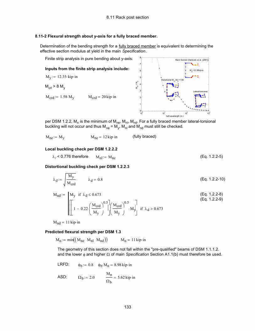
8.11 Rack post section
Distortional buckling check per DSM 1.2.2.3
λdMy
Mcrd:= λd 0.8= (Eq. 1.2.2-10)
Mnd My λd 0.673≤if
1 0.22Mcrd
My
0.5
⋅−
Mcrd
My
0.5
My⋅
λd 0.673>if
:= (Eq. 1.2.2-8)(Eq. 1.2.2-9)
Mnd 11 kip in⋅=
Predicted flexural strength per DSM 1.3
Mn min Mne Mnl Mnd( )( ):= Mn 11 kip in⋅=
The geometry of this section does not fall within the "pre-qualified" beams of DSM 1.1.1.2. and the lower φ and higher Ω of main Specification Section A1.1(b) must therefore be used.
LRFD: φb 0.8:= φb Mn⋅ 8.98 kip in⋅=
ASD: Ωb 2.0:=Mn
Ωb5.62 kip in⋅=
8.11-2 Flexural strength about y-axis for a fully braced member.
Determination of the bending strength for a fully braced member is equivalent to determining the effective section modulus at yield in the main Specification.
100
101
102
103
0
1
2
3
4
5
6
7
8
half-wavelength (in.)
Mcr
/ M
y
Rack Section (Hancock et al. (2001))
My=12.35kip-in.
Distortional Mcr/My=1.58
Lateral-torsional
Finite strip analysis in pure bending about y-axis:
Inputs from the finite strip analysis include:
My 12.35 kip⋅ in⋅:=
Mcrl > 8 My
Mcrd 1.58 My⋅:= Mcrd 20 kip in⋅=
per DSM 1.2.2, Mn is the minimum of Mne, Mnl, Mnd. For a fully braced member lateral-torsional buckling will not occur and thus Mne = My, Mnl and Mnd must still be checked.
Mne My:= Mne 12 kip in⋅= (fully braced)
Local buckling check per DSM 1.2.2.2
λl < 0.776 therefore Mnl Mne:= (Eq. 1.2.2-5)
133
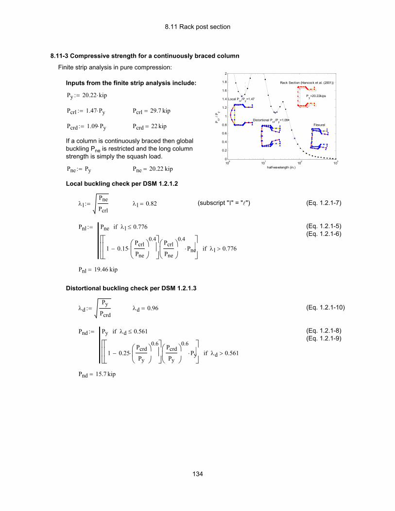
8.11 Rack post section
Pnd 15.7 kip=
(Eq. 1.2.1-8)(Eq. 1.2.1-9)
Pnd Py λd 0.561≤if
1 0.25Pcrd
Py
0.6
⋅−
Pcrd
Py
0.6
Py⋅
λd 0.561>if
:=
(Eq. 1.2.1-10)λd 0.96=λdPy
Pcrd:=
Distortional buckling check per DSM 1.2.1.3
Pnl 19.46 kip=
(Eq. 1.2.1-5)(Eq. 1.2.1-6)
Pnl Pne λl 0.776≤if
1 0.15Pcrl
Pne
0.4
⋅−
Pcrl
Pne
0.4
Pne⋅
λl 0.776>if
:=
(Eq. 1.2.1-7)(subscript "l" = "l")λl 0.82=λlPne
Pcrl:=
Local buckling check per DSM 1.2.1.2
Pne 20.22 kip=Pne Py:=
If a column is continuously braced then global buckling Pne is restricted and the long column strength is simply the squash load.
Pcrd 22 kip=Pcrd 1.09 Py⋅:=
Pcrl 29.7 kip=Pcrl 1.47 Py⋅:=
Py 20.22 kip⋅:=
Inputs from the finite strip analysis include:
Finite strip analysis in pure compression:
100 101 102 1030
0.2
0.4
0.6
0.8
1
1.2
1.4
1.6
1.8
2
half-wavelength (in.)
Pcr
/ P y
Rack Section (Hancock et al. (2001))
Py=20.22kipsLocal Pcr/Py=1.47
Distortional Pcr/Py=1.09Flexural
8.11-3 Compressive strength for a continuously braced column
134
8.11 Rack post section
Pn
Ωc7.8 kip=Ωc 2.0:=ASD:
φc Pn⋅ 12.5 kip=φc 0.8:=LRFD:
The geometry of this section falls outside the "pre-qualified" columns of DSM 1.1.1.1 and thus the lower φ and higher Ω of main Specification Section A1.1(b) must be used.
= 0.3?, no, NG0.40.594
0.67=D2/D
> 2, therefore NG1.220.594
2.05=b2/D
< 2.9, OK3.431.39
2.47=ho/bo
> 8, therefore NG0.5940.06
9.9=D/t
> 22, therefore NG1.390.06
23.17=bo/t
The analyzed section fails the test for pre-qualified columns. The small violations for ho/t, bo/t, and D/t may be deemed legitimate by engineering judgment since the parameters are well within the values tested in standard C-shaped specimens. However, since the details of the complex rack post stiffener also fall outside the bounds of the tested specimens it becomes dificult to argue that this specimen should use the pre-qualified φ and Ω values, instead the rational analysis values are appropriate.
> 51, therefore NG3.430.06
57.17=ho/t
For determining φ, check against the pre-qualified columns of Table 1.1.1-1 in DSM Section 1.1.1.1. In the pre-qualified rack uprights, the first flange lip, D, is always 90 degrees from the flange, in this example D is 45 degrees. Here we assume this minor change is not a violation of the pre-qualified columns since θ variation was investigated significantly in the reported lipped C-sections, and thus check against the rack uprights given in the table.
Pn 15.7 kip=Pn min Pne Pnl Pnd( )( ):=
Predicted compressive strength per DSM 1.2
(Continued) 8.11-3 Compressive strength for a continuously braced column
135
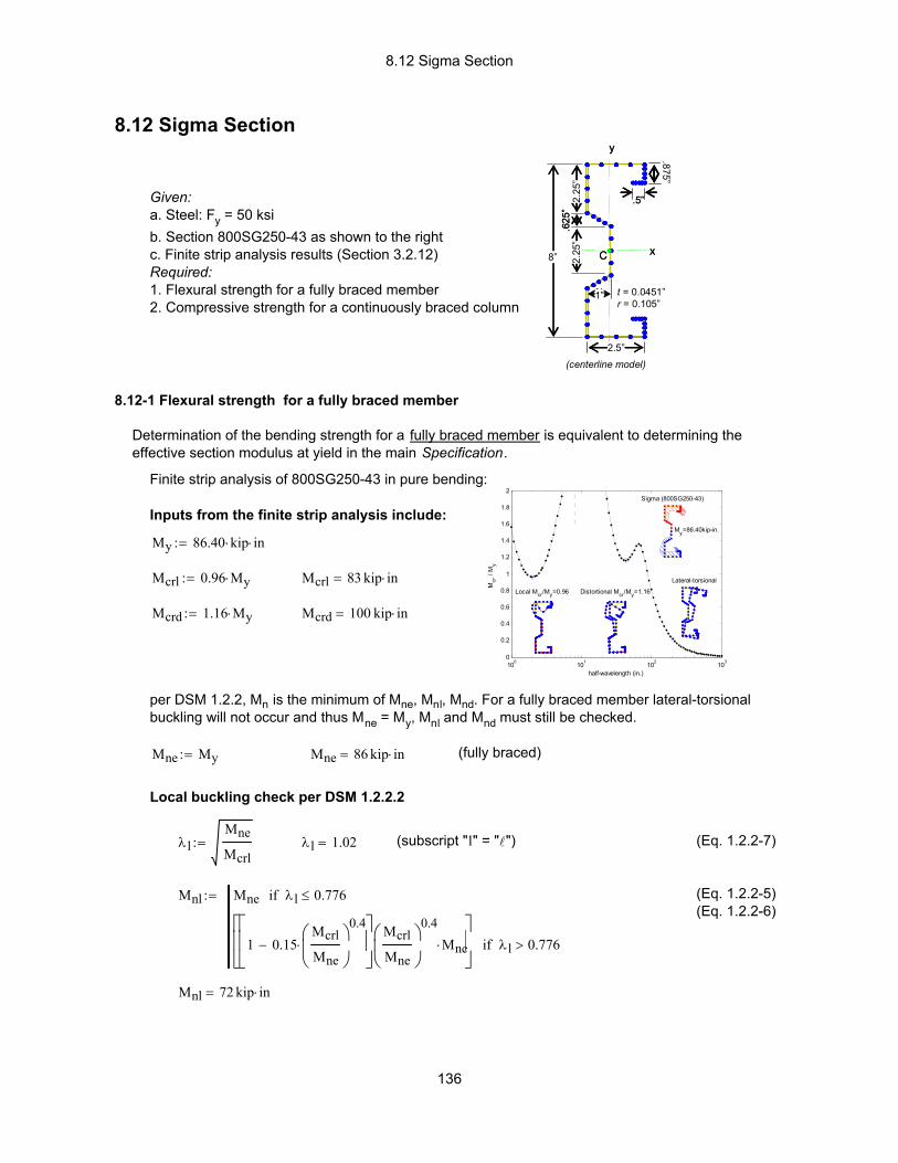
8.12 Sigma Section
Mnl 72 kip in⋅=
(Eq. 1.2.2-5)(Eq. 1.2.2-6)
Mnl Mne λl 0.776≤if
1 0.15Mcrl
Mne
0.4
⋅−
Mcrl
Mne
0.4
Mne⋅
λl 0.776>if
:=
(Eq. 1.2.2-7)(subscript "l" = "l")λl 1.02=λlMne
Mcrl:=
Local buckling check per DSM 1.2.2.2
(fully braced)Mne 86 kip in⋅=Mne My:=
per DSM 1.2.2, Mn is the minimum of Mne, Mnl, Mnd. For a fully braced member lateral-torsional buckling will not occur and thus Mne = My, Mnl and Mnd must still be checked.
Mcrd 100 kip in⋅=Mcrd 1.16 My⋅:=
Mcrl 83 kip in⋅=Mcrl 0.96 My⋅:=
My 86.40 kip⋅ in⋅:=
Inputs from the finite strip analysis include:
Finite strip analysis of 800SG250-43 in pure bending:
100 101 102 1030
0.2
0.4
0.6
0.8
1
1.2
1.4
1.6
1.8
2
half-wavelength (in.)
Mcr
/ M
y Sigma (800SG250-43)
My=86.40kip-in.
Local Mcr/My=0.96 Distortional Mcr/My=1.16
Lateral-torsional
Determination of the bending strength for a fully braced member is equivalent to determining the effective section modulus at yield in the main Specification.
8.12-1 Flexural strength for a fully braced member
Given: a. Steel: Fy = 50 ksib. Section 800SG250-43 as shown to the rightc. Finite strip analysis results (Section 3.2.12)Required:1. Flexural strength for a fully braced member2. Compressive strength for a continuously braced column
C x
y
8”
2.5”
2.25
”
1”
2.25
”
.875”
.5”
.625
”
t = 0.0451”r = 0.105”
(centerline model)
C x
y
8”
2.5”
2.25
”
1”
2.25
”
.875”
.5”
.625
”
t = 0.0451”r = 0.105”
(centerline model)
8.12 Sigma Section
136

8.12 Sigma Section
Mn
Ωb36 kip in⋅=Ωb 2.0:=ASD:
φb Mn⋅ 57 kip in⋅=φb 0.8:=LRFD:
The geometry of this section falls outside the "pre-qualified" beams of DSM 1.1.1.2 and the lower φ and higher Ω of main Specification Section A1.1(b) should be used.
Mn 71 kip in⋅=Mn min Mne Mnl Mnd( )( ):=
Predicted flexural strength per DSM 1.3
Mnd 71 kip in⋅=
(Eq. 1.2.2-8)(Eq. 1.2.2-9)
Mnd My λd 0.673≤if
1 0.22Mcrd
My
0.5
⋅−
Mcrd
My
0.5
My⋅
λd 0.673>if
:=
(Eq. 1.2.2-10)λd 0.93=λdMy
Mcrd:=
Distortional buckling check per DSM 1.2.2.3
(Continued) 8.12-1 Flexural strength for a fully braced member
137
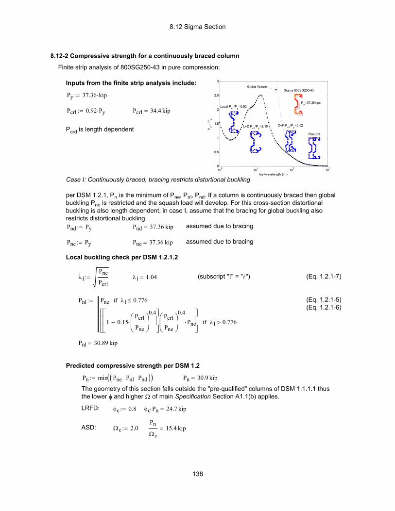
8.12 Sigma Section
λlPne
Pcrl:= λl 1.04= (subscript "l" = "l") (Eq. 1.2.1-7)
Pnl Pne λl 0.776≤if
1 0.15Pcrl
Pne
0.4
⋅−
Pcrl
Pne
0.4
Pne⋅
λl 0.776>if
:= (Eq. 1.2.1-5)(Eq. 1.2.1-6)
Pnl 30.89 kip=
Predicted compressive strength per DSM 1.2
Pn min Pne Pnl Pnd( )( ):= Pn 30.9 kip=
The geometry of this section falls outside the "pre-qualified" columns of DSM 1.1.1.1 thus the lower φ and higher Ω of main Specification Section A1.1(b) applies.
LRFD: φc 0.8:= φc Pn⋅ 24.7 kip=
ASD: Ωc 2.0:=Pn
Ωc15.4 kip=
8.12-2 Compressive strength for a continuously braced column
Finite strip analysis of 800SG250-43 in pure compression:
100 101 102 1030
0.5
1
1.5
2
2.5
3
half-wavelength (in.)
Pcr
/ P
y
Sigma 800SG250-43
Py=37.36kipsLocal Pcr/Py=0.92
L+D Pcr/Py=2.10 D+F Pcr/Py=0.52
Flexural
Global flexure Inputs from the finite strip analysis include:
Py 37.36 kip⋅:=
Pcrl 0.92 Py⋅:= Pcrl 34.4 kip=
Pcrd is length dependent
Case I: Continuously braced, bracing restricts distortional buckling
per DSM 1.2.1, Pn is the minimum of Pne, Pnl, Pnd. If a column is continuously braced then global buckling Pne is restricted and the squash load will develop. For this cross-section distortional buckling is also length dependent, in case I, assume that the bracing for global buckling also restricts distortional buckling. Pnd Py:= Pnd 37.36 kip= assumed due to bracing
Pne Py:= Pne 37.36 kip= assumed due to bracing
Local buckling check per DSM 1.2.1.2
138

8.12 Sigma Section
(inelastic regime) (Eq. 1.2.1-3)
Pne 0.658λ c
2
Py⋅ λc 1.5≤if
0.877
λc2
Py⋅ λc 1.5>if
:= (Eq. 1.2.1-1)
(Eq. 1.2.1-2)
Pne 24.98 kip=
Local buckling check per DSM 1.2.1.2 (this check is dependent on P ne)
λlPne
Pcrl:= λl 0.85= (subscript "l" = "l") (Eq. 1.2.1-7)
Pnl Pne λl 0.776≤if
1 0.15Pcrl
Pne
0.4
⋅−
Pcrl
Pne
0.4
Pne⋅
λl 0.776>if
:= (Eq. 1.2.1-5)
(Eq. 1.2.1-6)
Pnl 23.55 kip= Distortional buckling controls, but for longer unbraced length P nl soon controls.
Predicted compressive strength per DSM 1.2
Pn min Pne Pnl Pnd( )( ):= Pn 21 kip=
LRFD: φc 0.8:= φc Pn⋅ 16.8 kip= ASD: Ωc 2.0:=Pn
Ωc10.5 kip=
(continued) 8.12-2 Compressive strength for a continuously braced column
Case II: Discrete braces at 66 in. that restrict distortional and global buckling
Distortional buckling check per DSM 1.2.1.3
For a 66 in. unbraced length Pcrd from the FSM analysis is Pcrd 0.52 Py⋅:= , Pcrd 19.4 kip=
λdPy
Pcrd:= λd 1.39= (Eq. 1.2.1-10)
Pnd Py λd 0.561≤if
1 0.25Pcrd
Py
0.6
⋅−
Pcrd
Py
0.6
Py⋅
λd 0.561>if
:= (Eq. 1.2.1-8)(Eq. 1.2.1-9)
Pnd 21 kip= compare with Pnl from the continuously braced case, Pnl 30.89 kip=
At 66 in. unbraced length, Global buckling must also be calculated!
from the main Specification equations (see Section 2.6 of this Guide) or from FSM analysis (see Sections 3.3.4 and 3.3.5 of this Guide). Results from FSM analysis,
Pcre 1.04 Py⋅:= Pcre 38.85 kip= at 66 in.
Global buckling (long column strength) check per DSM 1.2.1.1
λcPy
Pcre:= λc 0.98=
139
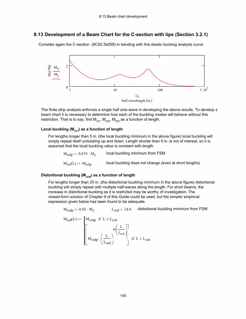
8.13 Beam chart development
Mcrd L( ) Mcrdp L Lcrd≥if
McrdpL
Lcrd
lnL
Lcrd
⋅
L Lcrd<if
:=
distortional buckling minimum from FSMLcrd 24.8:=Mcrdp 0.85 My⋅:=
For lengths longer than 25 in. (the distortional buckling minimum in the above figure) distortional buckling will simply repeat with multiple half-waves along the length. For short beams, the increase in distortional buckling as it is restricted may be worthy of investigation. The closed-form solution of Chapter 9 of this Guide could be used, but the simpler empirical expression given below has been found to be adequate.
Distortional buckling (Mcrd) as a function of length
local buckling does not change (even at short lengths)Mcrl L( ) Mcrlp:=
local buckling minimum from FSMMcrlp 0.674 My⋅:=
For lengths longer than 5 in. (the local buckling minimum in the above figure) local buckling will simply repeat itself undulating up and down. Length shorter than 5 in. is not of interest, so it is assumed that the local buckling value is constant with length.
Local buckling (Mcrl) as a function of length
The finite strip analysis enforces a single half sine wave in developing the above results. To develop abeam chart it is necessary to determine how each of the buckling modes will behave without this restriction. That is to say, find Mcrl, Mcrd, Mcre as a function of length.
1 10 100 1 .1030
2
half-wavelength (in.)
Mcr
/My Mcr
My
L2
Consider again the C-section (9CS2.5x059) in bending with this elastic bucking analysis curve:
8.13 Development of a Beam Chart for the C-section with lips (Section 3.2.1)
140
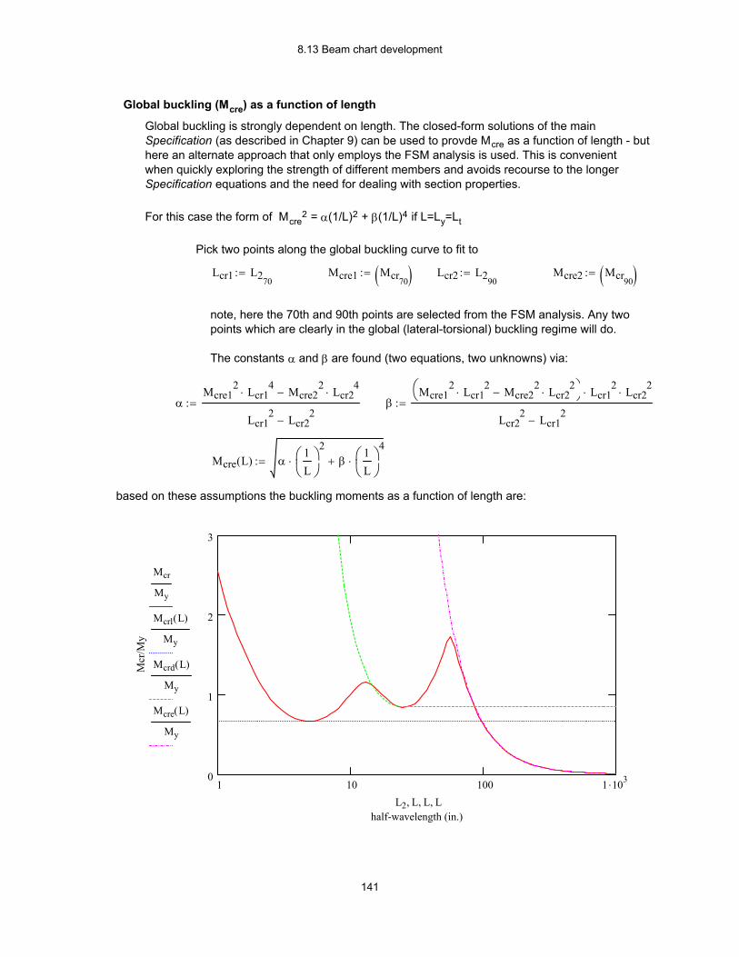
8.13 Beam chart development
Local
Distortional
Global (LTB)
1 10 100 1 .1030
1
2
3
half-wavelength (in.)
Mcr
/My
Mcr
My
Mcrl L( )
My
Mcrd L( )
My
Mcre L( )
My
L2 L, L, L,
based on these assumptions the buckling moments as a function of length are:
Mcre L( ) α1L
2⋅ β
1L
4⋅+:=
βMcre1
2 Lcr12
⋅ Mcre22 Lcr2
2⋅−
Lcr1
2⋅ Lcr2
2⋅
Lcr22 Lcr1
2−
:=αMcre1
2 Lcr14
⋅ Mcre22 Lcr2
4⋅−
Lcr12 Lcr2
2−
:=
The constants α and β are found (two equations, two unknowns) via:
note, here the 70th and 90th points are selected from the FSM analysis. Any two points which are clearly in the global (lateral-torsional) buckling regime will do.
Mcre2 Mcr90( ):=Lcr2 L290:=Mcre1 Mcr70( ):=Lcr1 L270
:=
Pick two points along the global buckling curve to fit to
Global buckling is strongly dependent on length. The closed-form solutions of the main Specification (as described in Chapter 9) can be used to provde Mcre as a function of length - but here an alternate approach that only employs the FSM analysis is used. This is convenient when quickly exploring the strength of different members and avoids recourse to the longer Specification equations and the need for dealing with section properties.
For this case the form of Mcre2 = α(1/L)2 + β(1/L)4 if L=Ly=Lt
Global buckling (Mcre) as a function of length
141
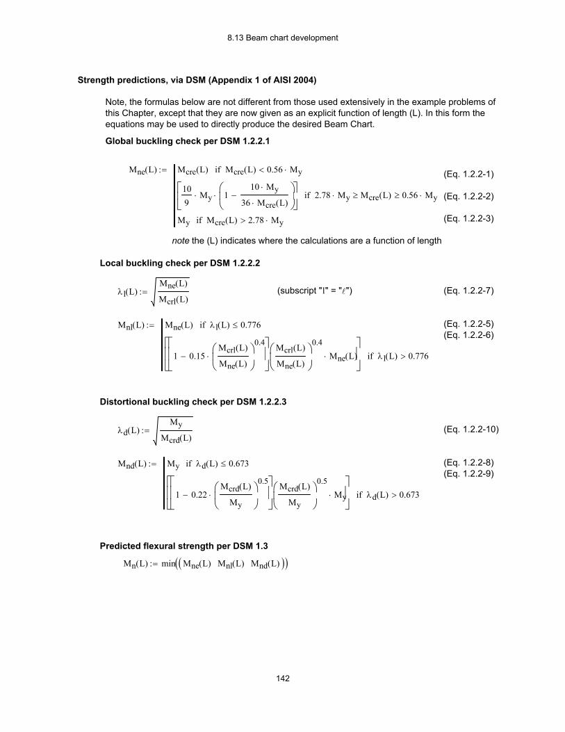
8.13 Beam chart development
Mn L( ) min Mne L( ) Mnl L( ) Mnd L( )( )( ):=
Predicted flexural strength per DSM 1.3
(Eq. 1.2.2-8)(Eq. 1.2.2-9)
Mnd L( ) My λd L( ) 0.673≤if
1 0.22Mcrd L( )
My
0.5
⋅−
Mcrd L( )
My
0.5
My⋅
λd L( ) 0.673>if
:=
(Eq. 1.2.2-10)λd L( )My
Mcrd L( ):=
Distortional buckling check per DSM 1.2.2.3
(Eq. 1.2.2-5)(Eq. 1.2.2-6)
Mnl L( ) Mne L( ) λl L( ) 0.776≤if
1 0.15Mcrl L( )
Mne L( )
0.4
⋅−
Mcrl L( )
Mne L( )
0.4
Mne L( )⋅
λl L( ) 0.776>if
:=
(Eq. 1.2.2-7)(subscript "l" = "l")λl L( )Mne L( )
Mcrl L( ):=
Local buckling check per DSM 1.2.2.2
note the (L) indicates where the calculations are a function of length
(Eq. 1.2.2-3)
(Eq. 1.2.2-2)
(Eq. 1.2.2-1)Mne L( ) Mcre L( ) Mcre L( ) 0.56 My⋅<if
109
My⋅ 110 My⋅
36 Mcre L( )⋅−
⋅
2.78 My⋅ Mcre L( )≥ 0.56 My⋅≥if
My Mcre L( ) 2.78 My⋅>if
:=
Global buckling check per DSM 1.2.2.1
Note, the formulas below are not different from those used extensively in the example problems of this Chapter, except that they are now given as an explicit function of length (L). In this form the equations may be used to directly produce the desired Beam Chart.
Strength predictions, via DSM (Appendix 1 of AISI 2004)
142

8.13 Beam chart development
Developed Beam Chart
DSM Beam Chart for the 9CS2.5x059
0 5 10 15 200
20
40
60
80
100
120
140
length (ft)
bend
ing
capa
city
(kip
-in.)
Mn L( )
Mne L( )
Mnl L( )
Mnd L( )
L
12
Mne
Mnd
Notes on the beam chart...(1) Distortional buckling (Mnd) controls the strength for a small group of lengths approximately between 2 and 5 ft.(2) Beyond approximately 10 ft. in length local buckling (Mnl) does not reduce the capacity below the global buckling strength (Mne) (In the parlance of the main Specification, this cross- section is fully effective for an unbraced length beyond 10 ft).
143
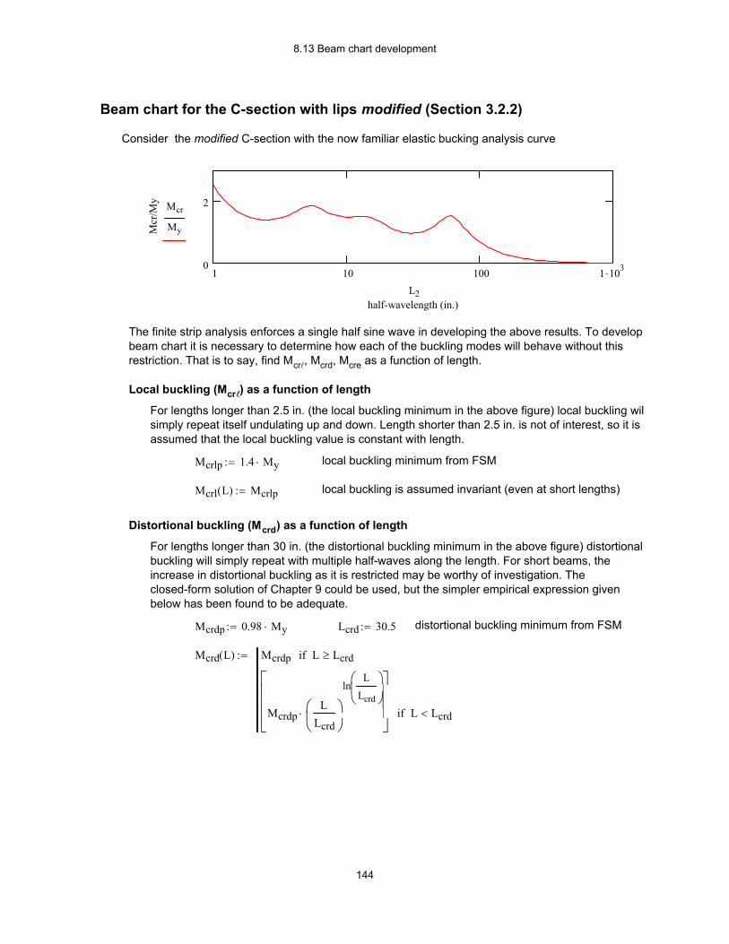
8.13 Beam chart development
Mcrd L( ) Mcrdp L Lcrd≥if
McrdpL
Lcrd
lnL
Lcrd
⋅
L Lcrd<if
:=
distortional buckling minimum from FSMLcrd 30.5:=Mcrdp 0.98 My⋅:=
For lengths longer than 30 in. (the distortional buckling minimum in the above figure) distortional buckling will simply repeat with multiple half-waves along the length. For short beams, the increase in distortional buckling as it is restricted may be worthy of investigation. The closed-form solution of Chapter 9 could be used, but the simpler empirical expression given below has been found to be adequate.
Distortional buckling (Mcrd) as a function of length
local buckling is assumed invariant (even at short lengths)Mcrl L( ) Mcrlp:=
local buckling minimum from FSMMcrlp 1.4 My⋅:=
For lengths longer than 2.5 in. (the local buckling minimum in the above figure) local buckling wilsimply repeat itself undulating up and down. Length shorter than 2.5 in. is not of interest, so it is assumed that the local buckling value is constant with length.
Local buckling (Mcrl) as a function of length
The finite strip analysis enforces a single half sine wave in developing the above results. To develop beam chart it is necessary to determine how each of the buckling modes will behave without this restriction. That is to say, find Mcrl, Mcrd, Mcre as a function of length.
1 10 100 1 .1030
2
half-wavelength (in.)
Mcr
/My Mcr
My
L2
Consider the modified C-section with the now familiar elastic bucking analysis curve
Beam chart for the C-section with lips modified (Section 3.2.2)
144
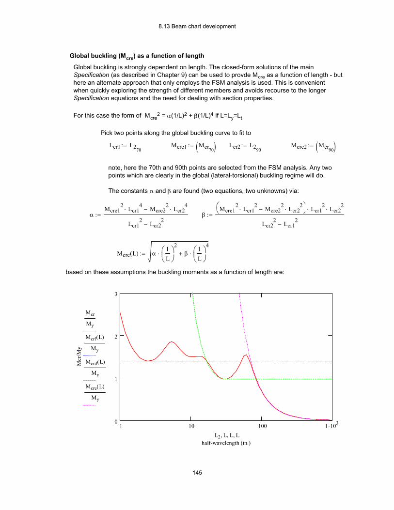
8.13 Beam chart development
Local
Distortional
Global (LTB)
1 10 100 1 .1030
1
2
3
half-wavelength (in.)
Mcr
/My
Mcr
My
Mcrl L( )
My
Mcrd L( )
My
Mcre L( )
My
L2 L, L, L,
based on these assumptions the buckling moments as a function of length are:
Mcre L( ) α1L
2⋅ β
1L
4⋅+:=
βMcre1
2 Lcr12
⋅ Mcre22 Lcr2
2⋅−
Lcr1
2⋅ Lcr2
2⋅
Lcr22 Lcr1
2−
:=αMcre1
2 Lcr14
⋅ Mcre22 Lcr2
4⋅−
Lcr12 Lcr2
2−
:=
The constants α and β are found (two equations, two unknowns) via:
note, here the 70th and 90th points are selected from the FSM analysis. Any two points which are clearly in the global (lateral-torsional) buckling regime will do.
Mcre2 Mcr90( ):=Lcr2 L290:=Mcre1 Mcr70( ):=Lcr1 L270
:=
Pick two points along the global buckling curve to fit to
Global buckling is strongly dependent on length. The closed-form solutions of the main Specification (as described in Chapter 9) can be used to provde Mcre as a function of length - but here an alternate approach that only employs the FSM analysis is used. This is convenient when quickly exploring the strength of different members and avoids recourse to the longer Specification equations and the need for dealing with section properties.
For this case the form of Mcre2 = α(1/L)2 + β(1/L)4 if L=Ly=Lt
Global buckling (Mcre) as a function of length
145
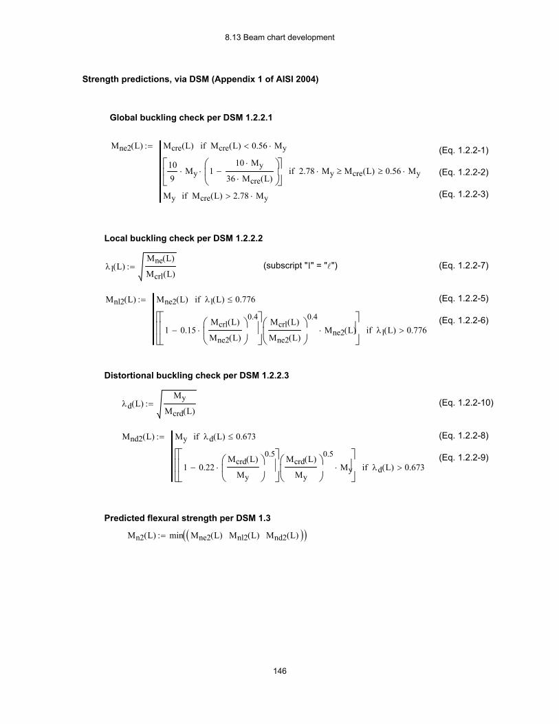
8.13 Beam chart development
Mn2 L( ) min Mne2 L( ) Mnl2 L( ) Mnd2 L( )( )( ):=
Predicted flexural strength per DSM 1.3
(Eq. 1.2.2-8)
(Eq. 1.2.2-9)
Mnd2 L( ) My λd L( ) 0.673≤if
1 0.22Mcrd L( )
My
0.5
⋅−
Mcrd L( )
My
0.5
My⋅
λd L( ) 0.673>if
:=
(Eq. 1.2.2-10)λd L( )My
Mcrd L( ):=
Distortional buckling check per DSM 1.2.2.3
(Eq. 1.2.2-5)
(Eq. 1.2.2-6)
Mnl2 L( ) Mne2 L( ) λl L( ) 0.776≤if
1 0.15Mcrl L( )
Mne2 L( )
0.4
⋅−
Mcrl L( )
Mne2 L( )
0.4
Mne2 L( )⋅
λl L( ) 0.776>if
:=
(Eq. 1.2.2-7)(subscript "l" = "l")λl L( )Mne L( )
Mcrl L( ):=
Local buckling check per DSM 1.2.2.2
(Eq. 1.2.2-3)
(Eq. 1.2.2-2)
(Eq. 1.2.2-1)Mne2 L( ) Mcre L( ) Mcre L( ) 0.56 My⋅<if
109
My⋅ 110 My⋅
36 Mcre L( )⋅−
⋅
2.78 My⋅ Mcre L( )≥ 0.56 My⋅≥if
My Mcre L( ) 2.78 My⋅>if
:=
Global buckling check per DSM 1.2.2.1
Strength predictions, via DSM (Appendix 1 of AISI 2004)
146
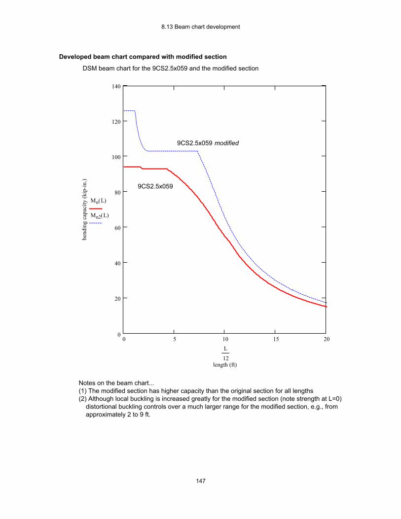
8.13 Beam chart development
Developed beam chart compared with modified section
DSM beam chart for the 9CS2.5x059 and the modified section
0 5 10 15 200
20
40
60
80
100
120
140
length (ft)
bend
ing
capa
city
(kip
-in.)
Mn L( )
Mn2 L( )
L
12
9CS2.5x059 modified
9CS2.5x059
Notes on the beam chart...(1) The modified section has higher capacity than the original section for all lengths(2) Although local buckling is increased greatly for the modified section (note strength at L=0) distortional buckling controls over a much larger range for the modified section, e.g., from approximately 2 to 9 ft.
147

8.13 Beam chart development
Developed beam chart compared with modified section (with resistance factors)
DSM beam chart for the 9CS2.5x059 and the modified section
0 5 10 15 200
10
20
30
40
50
60
70
80
90
100
110
length (ft)
desi
gn b
endi
ng c
apac
ity (k
ip-in
.)
0.9 Mn L( )
0.8 Mn2 L( )
L
12
9CS2.5x059 modified9CS2.5x059
Notes on the beam chart...(1) The lower resistance factor for the modified cross- section reduces the advantage of the modification, and over a short range of lengths actually provides less design strength than the original cross-section.(2) In the modified cross-section distortional buckling controls over a much larger length than in the original cross-section.
148
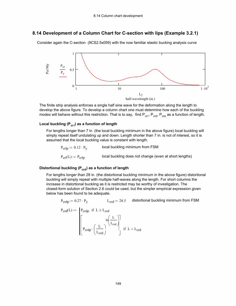
8.14 Column chart development
Pcrd L( ) Pcrdp L Lcrd≥if
PcrdpL
Lcrd
lnL
Lcrd
⋅
L Lcrd<if
:=
distortional buckling minimum from FSMLcrd 28.5:=Pcrdp 0.27 Py⋅:=
For lengths longer than 28 in. (the distortional buckling minimum in the above figure) distortional buckling will simply repeat with multiple half-waves along the length. For short columns the increase in distortional buckling as it is restricted may be worthy of investigation. The closed-form solution of Section 2.6 could be used, but the simpler empirical expression given below has been found to be adequate.
Distortional buckling (Pcrd) as a function of length
local buckling does not change (even at short lengths)Pcrl L( ) Pcrlp:=
local buckling minimum from FSMPcrlp 0.12 Py⋅:=
For lengths longer than 7 in. (the local buckling minimum in the above figure) local buckling will simply repeat itself undulating up and down. Length shorter than 7 in. is not of interest, so it is assumed that the local buckling value is constant with length.
Local buckling (Pcrl) as a function of length
The finite strip analysis enforces a single half sine wave for the deformation along the length to develop the above figure. To develop a column chart one must determine how each of the buckling modes will behave without this restriction. That is to say, find Pcrl, Pcrd, Pcre as a function of length.
1 10 100 1 .1030
0.5
1
half-wavelength (in.)
Pcr/M
y Pcr
Py
L2
Consider again the C-section (9CS2.5x059) with the now familiar elastic bucking analysis curve
8.14 Development of a Column Chart for C-section with lips (Example 3.2.1)
149

8.14 Column chart development
Local
Distortional
Global (Flexural)
1 10 100 1 .1030
0.2
0.4
0.6
0.8
half-wavelength (in.)
Mcr
/My
Pcr
Py
Pcrl L( )
Py
Pcrd L( )
Py
Pcre L( )
Py
L2 L, L, L,
based on these assumptions the buckling loads as a function of length are:
Pcre L( ) α1L
2⋅ β
1L
4⋅+:=
to identify the flexural mode as "flexural" (and not torsional-flexural) we must visually examine the mode shape.
βPcre1
2 Lcr12
⋅ Pcre22 Lcr2
2⋅−
Lcr1
2⋅ Lcr2
2⋅
Lcr22 Lcr1
2−
:=αPcre1
2 Lcr14
⋅ Pcre22 Lcr2
4⋅−
Lcr12 Lcr2
2−
:=
The constants α and β are found (two equations, two unknowns) via:
note, here the 70th and 90th points are selected from the FSM analysis. Any two points which are clearly in the global (lateral-torsional) buckling regime will do.
Pcre2 Pcr90( ):=Lcr2 L290:=Pcre1 Pcr70( ):=Lcr1 L270
:=
Pick two points along the global buckling curve to fit to
Global buckling is strongly dependent on length. The closed-form solutions of the main Specification (as demonstrated in Chapter 9) can be used to provde P cre as a function of length - but here an alternate approach that only employs the FSM analysis is used. This is convenient when quickly exploring the strength of different members and avoids recourse to the longer Specification equations and the need for dealing with section properties.
For this case the form of Pcre2 ~= α(1/L)2 + β(1/L)4 if L=Lx=Lt
Global buckling (Pcre) as a function of length
150
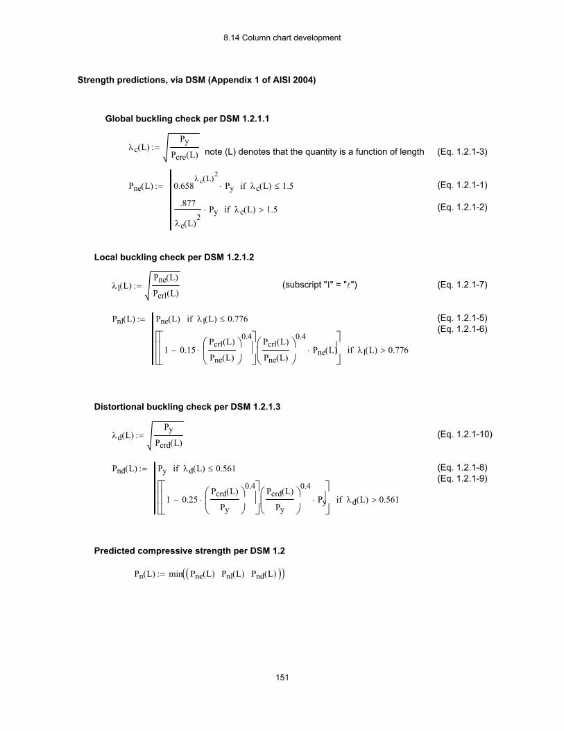
8.14 Column chart development
Pn L( ) min Pne L( ) Pnl L( ) Pnd L( )( )( ):=
Predicted compressive strength per DSM 1.2
(Eq. 1.2.1-8)(Eq. 1.2.1-9)
Pnd L( ) Py λd L( ) 0.561≤if
1 0.25Pcrd L( )
Py
0.4
⋅−
Pcrd L( )
Py
0.4
Py⋅
λd L( ) 0.561>if
:=
(Eq. 1.2.1-10)λd L( )Py
Pcrd L( ):=
Distortional buckling check per DSM 1.2.1.3
(Eq. 1.2.1-5)(Eq. 1.2.1-6)
Pnl L( ) Pne L( ) λl L( ) 0.776≤if
1 0.15Pcrl L( )
Pne L( )
0.4
⋅−
Pcrl L( )
Pne L( )
0.4
Pne L( )⋅
λl L( ) 0.776>if
:=
(Eq. 1.2.1-7)(subscript "l" = "l")λl L( )Pne L( )
Pcrl L( ):=
Local buckling check per DSM 1.2.1.2
(Eq. 1.2.1-2)
(Eq. 1.2.1-1)Pne L( ) 0.658λ c L( )2
Py⋅ λc L( ) 1.5≤if
.877
λc L( )2
Py⋅ λc L( ) 1.5>if
:=
(Eq. 1.2.1-3)note (L) denotes that the quantity is a function of lengthλc L( )Py
Pcre L( ):=
Global buckling check per DSM 1.2.1.1
Strength predictions, via DSM (Appendix 1 of AISI 2004)
151
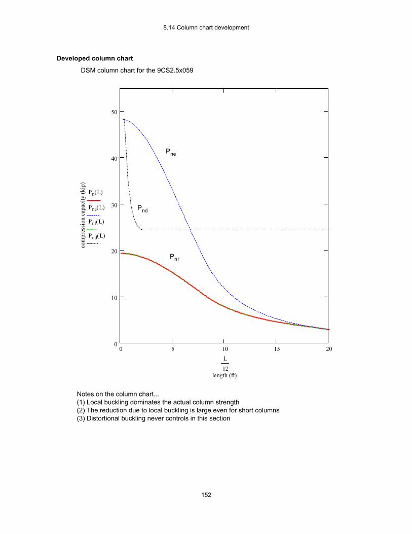
8.14 Column chart development
Developed column chart
DSM column chart for the 9CS2.5x059
0 5 10 15 200
10
20
30
40
50
length (ft)
com
pres
sion
cap
acity
(kip
)
Pn L( )
Pne L( )
Pnl L( )
Pnd L( )
L
12
Pne
Pnd
Pnl
Notes on the column chart...(1) Local buckling dominates the actual column strength(2) The reduction due to local buckling is large even for short columns(3) Distortional buckling never controls in this section
152
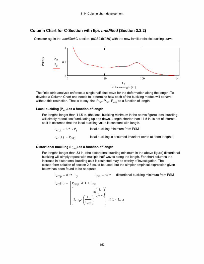
8.14 Column chart development
Pcrd L( ) Pcrdp L Lcrd≥if
PcrdpL
Lcrd
lnL
Lcrd
⋅
L Lcrd<if
:=
distortional buckling minimum from FSMLcrd 32.7:=Pcrdp 0.32 Py⋅:=
For lengths longer than 33 in. (the distortional buckling minimum in the above figure) distortional buckling will simply repeat with multiple half-waves along the length. For short columns the increase in distortional buckling as it is restricted may be worthy of investigation. The closed-form solution of section 2.5 could be used, but the simpler empirical expression given below has been found to be adequate.
Distortional buckling (Pcrd) as a function of length
local buckling is assumed invariant (even at short lengths)Pcrl L( ) Pcrlp:=
local buckling minimum from FSMPcrlp 0.27 Py⋅:=
For lengths longer than 11.5 in. (the local buckling minimum in the above figure) local buckling will simply repeat itself undulating up and down. Length shorter than 11.5 in. is not of interest, so it is assumed that the local buckling value is constant with length.
Local buckling (Pcrl) as a function of length
The finite strip analysis enforces a single half sine wave for the deformation along the length. To develop a Column Chart one needs to determine how each of the buckling modes will behave without this restriction. That is to say, find Pcrl, Pcrd, Pcre as a function of length.
1 10 100 1 .100
0.5
1
half-wavelength (in.)
Pcr/M
y Pcr
Py
L2
Consider again the modified C-section (9CS2.5x059) with the now familiar elastic bucking curve
Column Chart for C-Section with lips modified (Section 3.2.2)
153
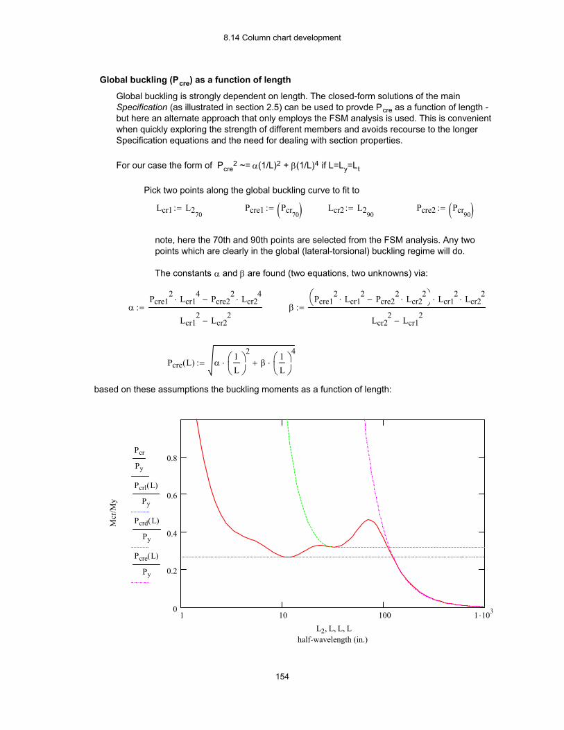
8.14 Column chart development
Local
Distortional
Global (LTB)
1 10 100 1 .1030
0.2
0.4
0.6
0.8
half-wavelength (in.)
Mcr
/My
Pcr
Py
Pcrl L( )
Py
Pcrd L( )
Py
Pcre L( )
Py
L2 L, L, L,
based on these assumptions the buckling moments as a function of length:
Pcre L( ) α1L
2⋅ β
1L
4⋅+:=
βPcre1
2 Lcr12
⋅ Pcre22 Lcr2
2⋅−
Lcr1
2⋅ Lcr2
2⋅
Lcr22 Lcr1
2−
:=αPcre1
2 Lcr14
⋅ Pcre22 Lcr2
4⋅−
Lcr12 Lcr2
2−
:=
The constants α and β are found (two equations, two unknowns) via:
note, here the 70th and 90th points are selected from the FSM analysis. Any two points which are clearly in the global (lateral-torsional) buckling regime will do.
Pcre2 Pcr90( ):=Lcr2 L290:=Pcre1 Pcr70( ):=Lcr1 L270
:=
Pick two points along the global buckling curve to fit to
Global buckling is strongly dependent on length. The closed-form solutions of the main Specification (as illustrated in section 2.5) can be used to provde Pcre as a function of length - but here an alternate approach that only employs the FSM analysis is used. This is convenient when quickly exploring the strength of different members and avoids recourse to the longer Specification equations and the need for dealing with section properties.
For our case the form of Pcre2 ~= α(1/L)2 + β(1/L)4 if L=Ly=Lt
Global buckling (Pcre) as a function of length
154
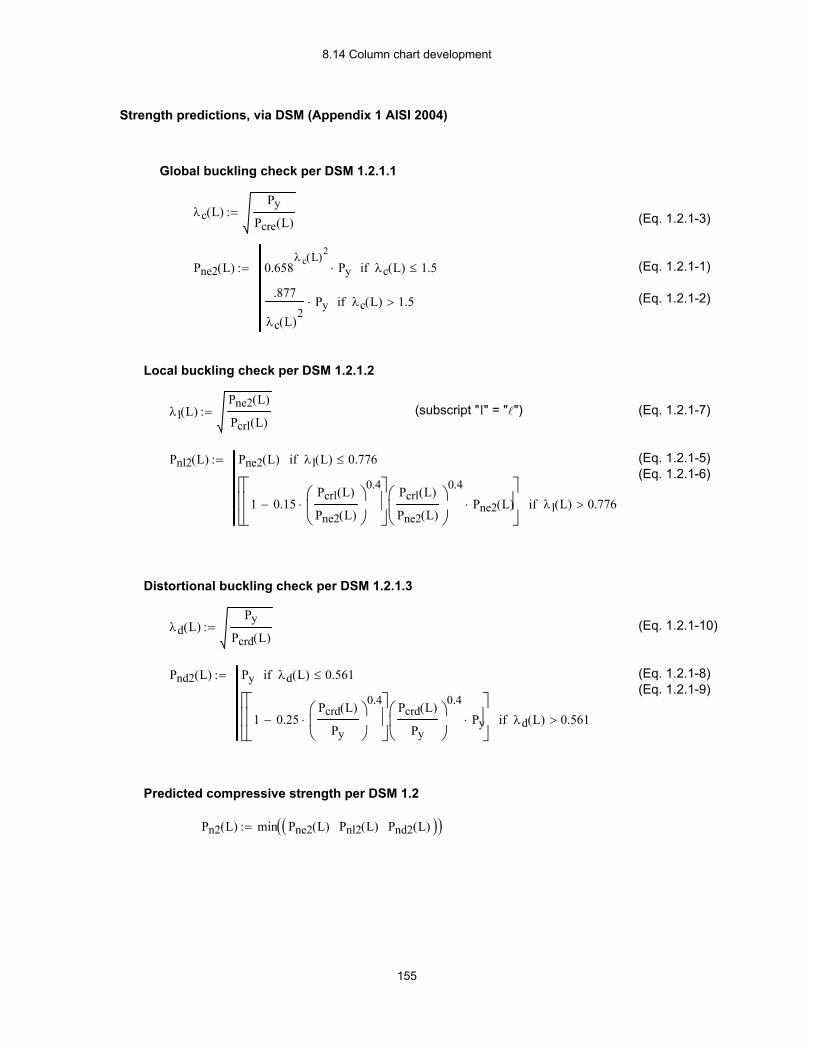
8.14 Column chart development
Pn2 L( ) min Pne2 L( ) Pnl2 L( ) Pnd2 L( )( )( ):=
Predicted compressive strength per DSM 1.2
(Eq. 1.2.1-8)(Eq. 1.2.1-9)
Pnd2 L( ) Py λd L( ) 0.561≤if
1 0.25Pcrd L( )
Py
0.4
⋅−
Pcrd L( )
Py
0.4
Py⋅
λd L( ) 0.561>if
:=
(Eq. 1.2.1-10)λd L( )Py
Pcrd L( ):=
Distortional buckling check per DSM 1.2.1.3
(Eq. 1.2.1-5)(Eq. 1.2.1-6)
Pnl2 L( ) Pne2 L( ) λl L( ) 0.776≤if
1 0.15Pcrl L( )
Pne2 L( )
0.4
⋅−
Pcrl L( )
Pne2 L( )
0.4
Pne2 L( )⋅
λl L( ) 0.776>if
:=
(Eq. 1.2.1-7)(subscript "l" = "l")λl L( )Pne2 L( )
Pcrl L( ):=
Local buckling check per DSM 1.2.1.2
(Eq. 1.2.1-2)
(Eq. 1.2.1-1)Pne2 L( ) 0.658λ c L( )2
Py⋅ λc L( ) 1.5≤if
.877
λc L( )2
Py⋅ λc L( ) 1.5>if
:=
(Eq. 1.2.1-3)λc L( )Py
Pcre L( ):=
Global buckling check per DSM 1.2.1.1
Strength predictions, via DSM (Appendix 1 AISI 2004)
155

8.14 Column chart development
Column Chart for the C-section with lips modifiedFollowing the same procedure as for the standard C-section a DSM Column Chart for the 9CS2.5x059 modified is generated and compared to the original 9CS2.5x059 C-section below.
0 5 10 15 200
5
10
15
20
25
30
35
40
45
50
55
length (ft)
com
pres
sion
cap
acity
(kip
)
Pn L( )
Pn2 L( )
Pnd2 L( )
Pne2 L( )
L
12
9CS2.5x059modified
9CS2.5x059
Notes on the column chart...(1) Local buckling dominates the strength, but the modified section is much improved(2) The modified section provides greater capacity at all lengths(3) Distortional buckling never controls in either section, but further improvement to local buckling without improvement to distortional buckling will not benefit this section much, because distortional buckling will begin to control.
156
157
8.15 Comparison of DSM with main Specification A comparison of the main Specification strength prediction and those of DSM Appendix 1 is provided in Table 6 for the example problems of this Chapter. In some cases the main Specification predictions are not applicable (designated N/A in the table) due to the unique geometry of the modified cross-sections, in other cases the AISI (2002) Design Manual does not provide a specific calculation and thus, none is given here (designated “-” in the table). Ease of calculation/modification: the design examples are intended to illustrate that when a numerical elastic buckling analysis tool such as CUFSM is available the Direct Strength Method requires less calculation and complexity than the main Specification. For example in the AISI (2002) Design Manual, presentation of the bending strength calculation for the C-section with lips takes 4½ pages and intermediate iterations are still left out; calculation for the bending strength of the same C-section is presented in under 2 pages in Section 8.1 of this Guide. More importantly a significant modification, including the addition of web stiffeners, still takes less than 2 pages to present the bending strength prediction as shown in Section 8.2 of this Guide. Slender elements: DSM discourages the use of very slender individual elements, as this drives the entire cross-section capacity down. For example, consider the compression capacity of the C-section with lips at Fn=37.25 ksi vs. the modified cross-section with web stiffeners added, as shown in Table 6: Pn=15.2 kips unmodified and 21.6 kips modified. This 42% improvement in strength comes solely from the addition of two small ¼ in. web stiffeners in the otherwise very slender web. When local buckling controls the strength small changes in the geometry are rewarded generously by DSM, less so by the main Specification. Distortional buckling: the last column of Table 6 indicates which mode controlled the strength prediction in the DSM method, in a number of cases distortional buckling controls. The main Specification does not include an explicit check for distortional buckling, therefore it is anticipated that DSM may provide lower strength predictions in these cases. Indeed, where direct comparisons are available this is the case: DSM predictions where distortional buckling controls are lower than those of the main Specification. If bracing partially restricts distortional buckling, which is sometimes the case in practice, this may be included in the elastic buckling analysis (see Section 3.3.7 of this Guide). In this situation Mcrd or Pcrd may be elevated to the point at which it no longer controls. Though not currently included, the addition of a distortional buckling provision to the main Specification is a future possibility, and would eliminate this difference. Local buckling: DSM predicts that local buckling is more likely to control the strength in compression than in bending. This is due to the use of relatively slender webs in standard cross-sections. For cross-sections which are modified, or optimized, local buckling is generally less likely to control the fully braced strength in compression or bending, and instead distortional buckling controls. Modifications to increase local buckling are usually relatively simple, a corrugation or stiffener will do, while modifications for distortional buckling generally are more involved. For cross-sections where local-global interaction is considered through the use of applied stresses Fn less than Fy, local buckling often controls the strength. Even though DSM includes an explicit check on distortional buckling, and the main Specification does not. For many practical unbraced lengths local-global interaction governs the capacity and the main Specification’s lack of a distortional buckling check is irrelevant.
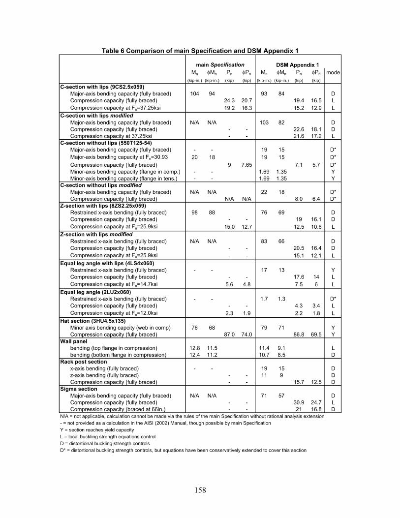
158
Table 6 Comparison of main Specification and DSM Appendix 1
main Specification DSM Appendix 1 Mn φMn Pn φPn Mn φMn Pn φPn mode
(kip-in.) (kip-in.) (kip) (kip) (kip-in.) (kip-in.) (kip) (kip)C-section with lips (9CS2.5x059)
Major-axis bending capacity (fully braced) 104 94 93 84 DCompression capacity (fully braced) 24.3 20.7 19.4 16.5 LCompression capacity at Fn=37.25ksi 19.2 16.3 15.2 12.9 L
C-section with lips modified Major-axis bending capacity (fully braced) N/A N/A 103 82 DCompression capacity (fully braced) - - 22.6 18.1 DCompression capacity at 37.25ksi - - 21.6 17.2 L
C-section without lips (550T125-54)Major-axis bending capacity (fully braced) - - 19 15 D*Major-axis bending capacity at Fn=30.93 20 18 19 15 D*Compression capacity (fully braced) 9 7.65 7.1 5.7 D*Minor-axis bending capacity (flange in comp.) - - 1.69 1.35 YMinor-axis bending capacity (flange in tens.) - - 1.69 1.35 Y
C-section without lips modifiedMajor-axis bending capacity (fully braced) N/A N/A 22 18 D*Compression capacity (fully braced) N/A N/A 8.0 6.4 D*
Z-section with lips (8ZS2.25x059)Restrained x-axis bending (fully braced) 98 88 76 69 DCompression capacity (fully braced) - - 19 16.1 DCompression capacity at Fn=25.9ksi 15.0 12.7 12.5 10.6 L
Z-section with lips modifiedRestrained x-axis bending (fully braced) N/A N/A 83 66 DCompression capacity (fully braced) - - 20.5 16.4 DCompression capacity at Fn=25.9ksi - - 15.1 12.1 L
Equal leg angle with lips (4LS4x060)Restrained x-axis bending (fully braced) - - 17 13 YCompression capacity (fully braced) - - 17.6 14 LCompression capacity at Fn=14.7ksi 5.6 4.8 7.5 6 L
Equal leg angle (2LU2x060)Restrained x-axis bending (fully braced) - - 1.7 1.3 D*Compression capacity (fully braced) - - 4.3 3.4 LCompression capacity at Fn=12.0ksi 2.3 1.9 2.2 1.8 L
Hat section (3HU4.5x135)Minor axis bending capcity (web in comp) 76 68 79 71 YCompression capacity (fully braced) 87.0 74.0 86.8 69.5 Y
Wall panelbending (top flange in compression) 12.8 11.5 11.4 9.1 Lbending (bottom flange in compression) 12.4 11.2 10.7 8.5 D
Rack post sectionx-axis bending (fully braced) - - 19 15 Dz-axis bending (fully braced) - - 11 9 DCompression capacity (fully braced) - - 15.7 12.5 D
Sigma sectionMajor-axis bending capacity (fully braced) N/A N/A 71 57 DCompression capacity (fully braced) - - 30.9 24.7 LCompression capacity (braced at 66in.) - - 21 16.8 D
N/A = not applicable, calculation cannot be made via the rules of the main Specification without rational analysis extension- = not provided as a calculation in the AISI (2002) Manual, though possible by main SpecificationY = section reaches yield capacityL = local buckling strength equations controlD = distortional buckling strength controlsD* = distortional buckling strength controls, but equations have been conservatively extended to cover this section
159
Lip stiffeners and Specification versus DSM: the main Specification and DSM Appendix 1 do not give the same optimum cross-sections. For example, with regard to lip stiffener length, the main Specification generally discourages long lip stiffeners, and thus those used in practice are relatively short. However, DSM (supported by testing, e.g., see Schafer 2002) encourages significantly longer lip stiffeners and rewards these cross-sections with higher capacities, particularly with regard to distortional buckling. Equal leg angle with lips: the DSM and main Specification predictions for the equal leg angle with lips, Section 3.2.7, provide fundamentally different results: Pn = 5.6 kips vs. 7.5 kips. This is due to the different ways that distortional buckling is handled for this cross-section. In the main Specification the edge stiffener provisions are invoked (a partial accounting for distortional buckling) and the effective width of the angle legs is reduced. In the DSM example problem, based on the finite strip analysis, it is recognized that distortional buckling of this cross-section is not distinct from torsional buckling, for a fully braced column the only reduction occurs from local buckling, not distortional. For a given unbraced length, the DSM method would include local-global interaction that would further reduce the capacity, but for a fully braced column, as computed in the example, no such reduction is relevant. Long beams and columns: global buckling is not investigated in detail in this comparison since DSM and the main Specification use identical strength expressions for determining the global beam or column strength. For longer unbraced lengths this dominates the results and the two methods yield the same strength prediction. However, for intermediate unbraced lengths, DSM includes an explicit distortional buckling check, and handles local-global interaction in a different manner; as such, the predictions by the two methods can diverge in this range. Rational analysis vs. pre-qualified: Many of the cross-sections analyzed with the Direct Strength Method do not meet the pre-qualified geometry, and as a result must use lower φ and higher Ω factors. This situation may tend to distort the optimal design, in the sense that the nominal strength may indicate that the addition of a web stiffener is highly beneficial, but the design strength does not – since the cross-section is no longer pre-qualified. Additional discussion on pre-qualified members can be found in Sections 1.3.2 and 7.4 of this Guide. Z-section and Z-section modified: The main Specification provides strength predictions for Z-sections that are higher than those of the Direct Strength Method for a fully braced cross-section. This is primarily due to the inclusion of un-restrained distortional buckling in the DSM calculation. If distortional buckling is restrained the prediction by the two methods is similar. As Table 6 shows, the main Specification and DSM (Appendix 1) provide similar, but different predictions for the strength. Since the methodologies are different, the optimal design (highest strength) that the two methods implicitly encourage is also different. DSM’s advantages lie in the ease of calculation and the ability to confidently examine variations in cross-section, while the main Specification provides a more prescriptive design methodology.
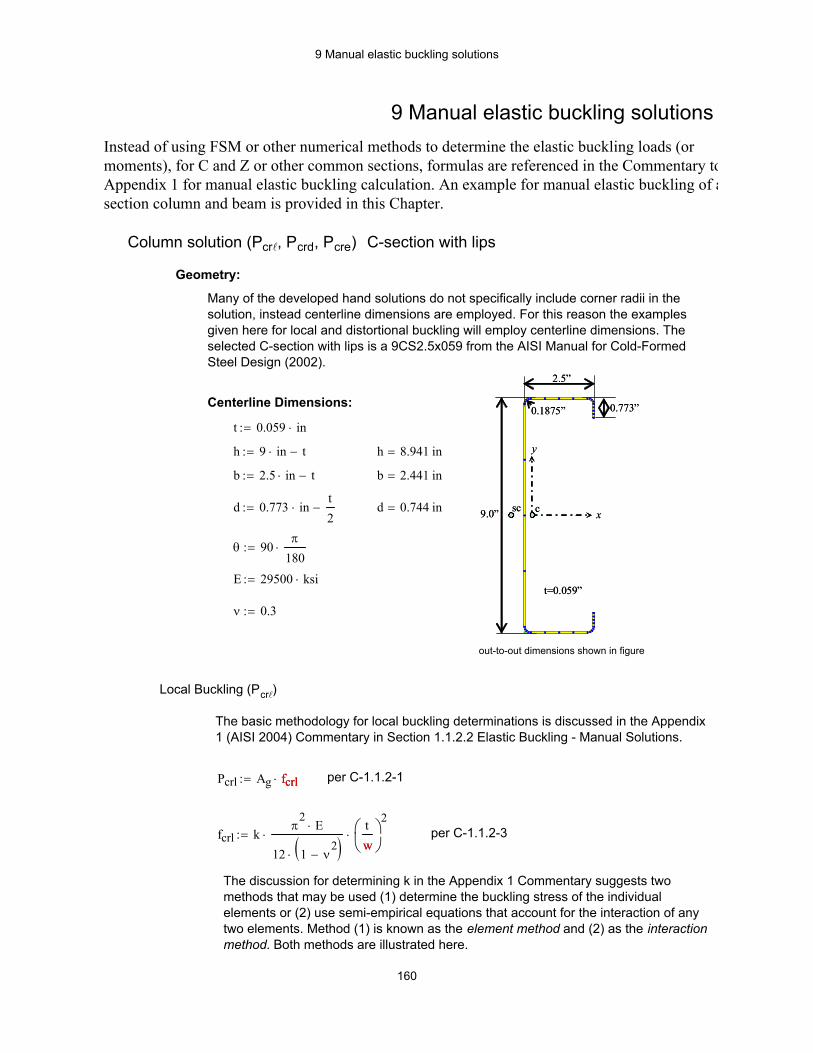
9 Manual elastic buckling solutions
The discussion for determining k in the Appendix 1 Commentary suggests two methods that may be used (1) determine the buckling stress of the individual elements or (2) use semi-empirical equations that account for the interaction of any two elements. Method (1) is known as the element method and (2) as the interaction method. Both methods are illustrated here.
per C-1.1.2-3fcrl kπ
2E⋅
12 1 ν2
−( )⋅
⋅tw
2⋅:=
w
per C-1.1.2-1Pcrl Ag fcrl⋅:= fcrl
The basic methodology for local buckling determinations is discussed in the Appendix 1 (AISI 2004) Commentary in Section 1.1.2.2 Elastic Buckling - Manual Solutions.
Local Buckling (Pcrl)
out-to-out dimensions shown in figure
ν 0.3:=
E 29500 ksi⋅:=
θ 90π
180⋅:=
d 0.744 in=d 0.773 in⋅t2
−:=
b 2.441 in=b 2.5 in⋅ t−:=
h 8.941 in=h 9 in⋅ t−:=
t 0.059 in⋅:=
Centerline Dimensions:
9.0”
2.5”
0.773”
t=0.059”
0.1875”
x
y
csc9.0”
2.5”
0.773”
t=0.059”
0.1875”
x
y
csc
Many of the developed hand solutions do not specifically include corner radii in the solution, instead centerline dimensions are employed. For this reason the examples given here for local and distortional buckling will employ centerline dimensions. The selected C-section with lips is a 9CS2.5x059 from the AISI Manual for Cold-Formed Steel Design (2002).
Geometry:
C-section with lipsColumn solution (Pcrl, Pcrd, Pcre)
Instead of using FSM or other numerical methods to determine the elastic buckling loads (or moments), for C and Z or other common sections, formulas are referenced in the Commentary toAppendix 1 for manual elastic buckling calculation. An example for manual elastic buckling of asection column and beam is provided in this Chapter.
9 Manual elastic buckling solutions
160

9 Manual elastic buckling solutions
Pcrl 4.195 kip=Pcrl Ag fcrl⋅:=
(using centerline dimensions)
Ag 0.903 in2=Ag h 2 b⋅+ 2 d⋅+( ) t⋅:=
fcrl 4.644 ksi=fcrl min fcr_flange fcr_web fcr_lip( )( ):=
fcr_lip 71.356 ksi=fcr_lip klipπ
2E⋅
12 1 ν2
−( )⋅
⋅td
2⋅:=
(per Table C-B2-1)klip 0.425:=
Classical solution for a plate simply-supported on three sides and free along one edgeis employed.
Lip Local Buckling:
fcr_web 4.644 ksi=fcr_web kwebπ
2E⋅
12 1 ν2
−( )⋅
⋅th
2⋅:=
(per Table C-B2-1)kweb 4:=
Classical solution for a simply-supported plate in pure compression is employed.
Web Local Buckling:
fcr_flange 62.306 ksi=fcr_flange kflangeπ
2E⋅
12 1 ν2
−( )⋅
⋅tb
2⋅:=
(per Table C-B2-1)kflange 4:=
Classical solution for a simply-supported plate in pure compression is employed.
Flange Local Buckling:
Element Method:
Local Buckling (Pcrl) (continued)
161
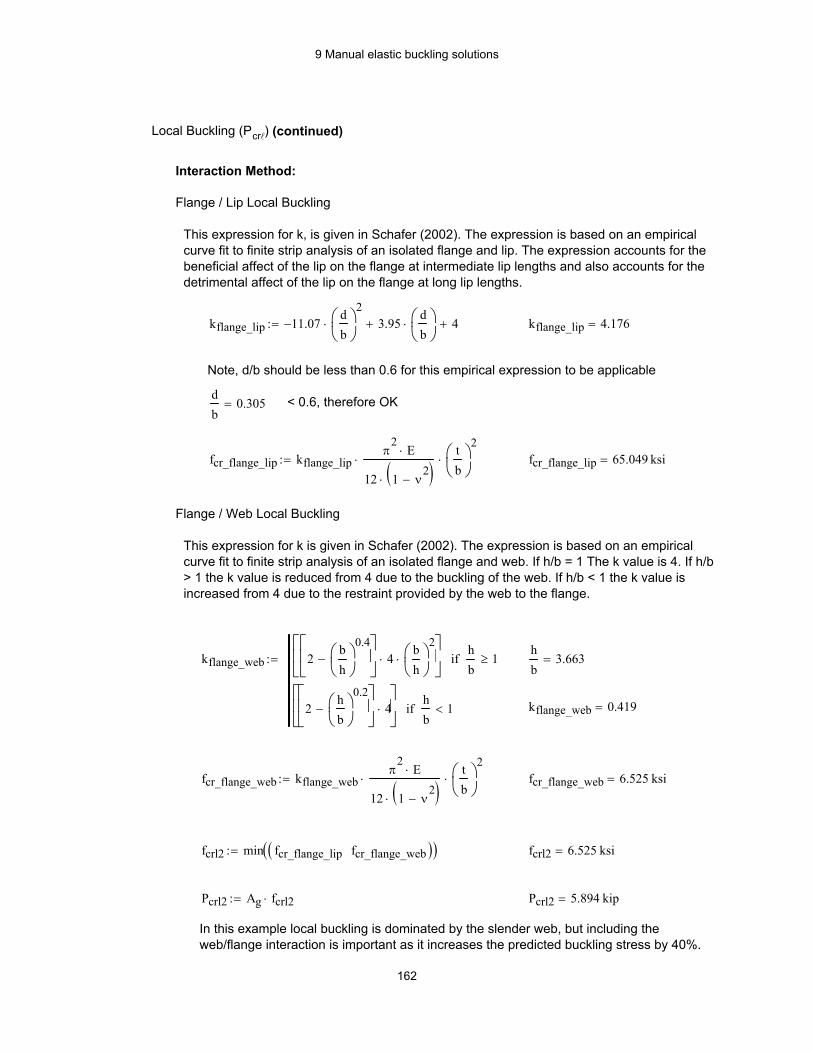
9 Manual elastic buckling solutions
In this example local buckling is dominated by the slender web, but including the web/flange interaction is important as it increases the predicted buckling stress by 40%.
Pcrl2 5.894 kip=Pcrl2 Ag fcrl2⋅:=
fcrl2 6.525 ksi=fcrl2 min fcr_flange_lip fcr_flange_web( )( ):=
fcr_flange_web 6.525 ksi=fcr_flange_web kflange_webπ
2E⋅
12 1 ν2
−( )⋅
⋅tb
2⋅:=
kflange_web 0.419=
hb
3.663=kflange_web 2bh
0.4−
4⋅bh
2⋅
hb
1≥if
2hb
0.2−
4⋅
hb
1<if
:=
This expression for k is given in Schafer (2002). The expression is based on an empirical curve fit to finite strip analysis of an isolated flange and web. If h/b = 1 The k value is 4. If h/b > 1 the k value is reduced from 4 due to the buckling of the web. If h/b < 1 the k value is increased from 4 due to the restraint provided by the web to the flange.
Flange / Web Local Buckling
fcr_flange_lip 65.049 ksi=fcr_flange_lip kflange_lipπ
2E⋅
12 1 ν2
−( )⋅
⋅tb
2⋅:=
< 0.6, therefore OKdb
0.305=
Note, d/b should be less than 0.6 for this empirical expression to be applicable
kflange_lip 4.176=kflange_lip 11.07−db
2⋅ 3.95
db
⋅+ 4+:=
This expression for k, is given in Schafer (2002). The expression is based on an empirical curve fit to finite strip analysis of an isolated flange and lip. The expression accounts for the beneficial affect of the lip on the flange at intermediate lip lengths and also accounts for the detrimental affect of the lip on the flange at long lip lengths.
Flange / Lip Local Buckling
Interaction Method:
Local Buckling (Pcrl) (continued)
162

9 Manual elastic buckling solutions
Ixyf 0.015 in4=
Ioft b3⋅
3b t3⋅
12+
t d3⋅
3+:= Iof 0.294 in4
=
x distance from the centroid tothe shear center.xof
b2 d2 cos θ( )⋅−
2 b d+( )⋅:= xof 0.936 in=
y distance from the centroid tothe shear center.yof
d2− sin θ( )⋅
2 b d+( )⋅:= yof 0.087− in=
x distance from the centroidto the web/flange juncture.hxf
b2 2 d⋅ b⋅+ d2 cos θ( )⋅+( )−
2 b d+( ):= hxf 1.505− in=
y distance from the centroidto the web/flange juncture.hyf
d2− sin θ( )⋅
2 b d+( )⋅:= hyf 0.087− in=
Cwf 0 in6⋅:= Cwf 0 in6
=
Distortional Buckling (Pcrd)
The basic methodology for distortional buckling determination is discussed in the Appendix 1 (AISI 2004) Commentary in Section 1.1.2.2 Elastic Buckling - Manual Solutions.
Pcrd Ag fcrd⋅:= fcrd per C-1.1.2-3
The method illustrated here is based on Schafer (2002). Section properties of the isolated flange must be calculated. The expressions here are only applicable for simple lips. More complicated flanges would follow the same procedure, but new expressions would be required.
x
y
xo
yo
hx
hyW/F
C
S Material Properties:
GE
2 1 ν+( )⋅:=
Properties of the Flange Only:
Af b d+( ) t⋅:= Af 0.188 in2=
Jf13
b⋅ t3⋅13
d⋅ t3⋅+:= Jf 2.18 10 4−× in4
=
Ixft t2 b2
⋅ 4 b⋅ d3⋅+ 4 b⋅ d3
⋅ cos θ( )2⋅− t2 b⋅ d⋅+ d4+ d4 cos θ( )2⋅−( )⋅
12 b d+( )⋅:= Ixf 6.709 10 3−
× in4=
Iyft b4 4 d⋅ b3
⋅+ 6 d2⋅ b2
⋅ cos θ( )⋅+ 4 d3⋅ b⋅ cos θ( )2⋅+ d4 cos θ( )2⋅+( )⋅
12 b d+( )⋅:= Iyf 0.122 in4
=
Ixyft b⋅ d2
⋅ sin θ( )⋅ b d cos θ( )⋅+( )⋅
4 b d+( )⋅:=
163
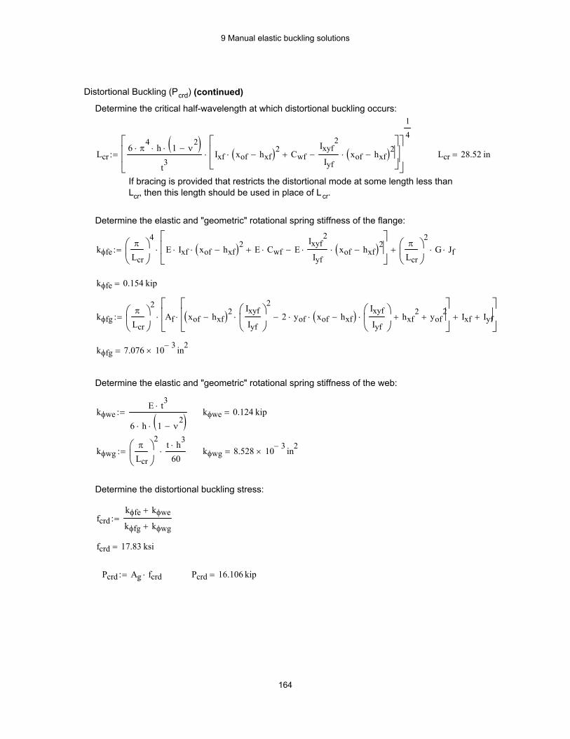
9 Manual elastic buckling solutions
Pcrd 16.106 kip=Pcrd Ag fcrd⋅:=
fcrd 17.83 ksi=
fcrdkφfe kφwe+
kφfg kφwg+:=
Determine the distortional buckling stress:
kφwg 8.528 10 3−× in2
=kφwgπ
Lcr
2t h3⋅
60⋅:=
kφwe 0.124 kip=kφweE t3⋅
6 h⋅ 1 ν2
−( )⋅
:=
Determine the elastic and "geometric" rotational spring stiffness of the web:
kφfg 7.076 10 3−× in2
=
kφfgπ
Lcr
2Af xof hxf−( )2
Ixyf
Iyf
2
⋅ 2 yof⋅ xof hxf−( )⋅Ixyf
Iyf
⋅− hxf
2+ yof
2+
⋅ Ixf+ Iyf+
⋅:=
kφfe 0.154 kip=
kφfeπ
Lcr
4E Ixf⋅ xof hxf−( )2⋅ E Cwf⋅+ E
Ixyf2
Iyf⋅ xof hxf−( )2⋅−
⋅π
Lcr
2G⋅ Jf⋅+:=
Determine the elastic and "geometric" rotational spring stiffness of the flange:
If bracing is provided that restricts the distortional mode at some length less thanLcr, then this length should be used in place of Lcr.
Lcr 28.52 in=Lcr6 π
4⋅ h⋅ 1 ν
2−( )⋅
t3Ixf xof hxf−( )2⋅ Cwf+
Ixyf2
Iyfxof hxf−( )2⋅−
⋅
1
4
:=
Determine the critical half-wavelength at which distortional buckling occurs:
Distortional Buckling (Pcrd) (continued)
164

9 Manual elastic buckling solutions
Ly 8 ft⋅:= Lt 8 ft⋅:=
individual buckling modes, per C3.1.2
σexπ
2E⋅
Kx Lx⋅
rx
2:= σey
π2
E⋅
Ky Ly⋅
ry
2:=(Eq. C3.1.2.1-7) (Eq. C3.1.2.1-8)
σex 369.352 ksi= σey 25.03 ksi=
σ t1
A ro2
⋅G J⋅
π2
E⋅ Cw⋅
Kt Lt⋅( )2+
⋅:= σ t 28.864 ksi= (Eq. C3.1.2.1-9)
torsional-flexural buckling per C4.2
Fe1
2 β⋅σex σ t+( ) σex σ t+( )2 4 β⋅ σex⋅ σ t⋅−−
⋅:= Fe 28.435 ksi= (Eq. C4.2-1)
note, for singly symmetric sections the x-axis is assumed to be the axis of symmetry
Fe2 σey:= note, Fe2 is compared with Fe to determine the minimum buckling stress per the note in C4.2. If ry is the least radius of gyration then Fe2 is defined as given, otherwise Fe2 should be calculated per the least radius of gyration, per C4.1
Fcre min Fe Fe2( )( ):= Fcre 25.03 ksi=
Global buckling (Pcre)
Global cross-section properties are given for this section in AISI Design Manual (2002), Example I-1: C-Section With Lips - Gross Section Properties
A 0.881 in2⋅:= Ix 10.3 in4
⋅:= Iy 0.698 in4⋅:=
J 0.00102 in4⋅:= Cw 11.9 in6
⋅:= xo 1.66− in⋅:=
rxIxA
:= rx 3.419 in= ryIyA
:= ry 0.89 in=
ro rx2 ry
2+ xo
2+:= ro 3.904 in= (Eq. C3.1.2.1-12)
β 1xo
ro
2
−:= β 0.819= (Eq. C4.2-3)
Length and bracing conditions (for example...)
Kx 1:= Ky 1:= Kt 1:=
Lx 8 ft⋅:=
165

9 Manual elastic buckling solutions
Web Local Buckling:
Classical solution for a simply-supported plate in pure bending is employed.
kweb 23.9:= (per Table C-B2-1)
fcr_web kwebπ
2E⋅
12 1 ν2
−( )⋅
⋅th
2⋅:= fcr_web 27.748 ksi=
Lip Local Buckling:
Based on the work in Schafer and Pekoz (1999) the influence of the stress gradient on the lip can be accounted for (otherwise use k=0.425 and ignore the stress gradient on the lip).
f1 1:= stress at the extreme fiber f2c d−
c:= f2 0.835= stress at end of lip
ξf1 f2−
f1:= ξ 0.165= klip 1.4 ξ
2⋅ 0.25 ξ⋅− 0.425+:= klip 0.422=
clearly in this case the stress gradient on the lip is of little significance as k~0.425
fcr_lip klipπ
2E⋅
12 1 ν2
−( )⋅
⋅td
2⋅:= fcr_lip 70.838 ksi=
Pcre A Fcre⋅:= Pcre 22.051 kip=
Beam solution (Mcrl, Mcrd, Mcre)
C-section with lips
Local Buckling (Mcrl) The basic methodology for local buckling is discussed in the Appendix 1 Commentary in Section 1.1.2.2 Elastic Buckling - Manual Solutions.
Mcrl Sg fcrl⋅:= Sg per C-1.1.2-2 where Sg=Ix/c and ch2
t2
+:= c 4.5 in=
fcrl kπ
2E⋅
12 1 ν2
−( )⋅
⋅tw
2⋅:=
wper C-1.1.2-3
For local buckling k may be determined by the element method or the interaction method. Both methods are illustrated here.
Element Method:
Flange Local Buckling:
Classical solution for a simply-supported plate in pure compression is employed.
kflange 4:= (per Table C-B2-1)
fcr_flange kflangeπ
2E⋅
12 1 ν2
−( )⋅
⋅tb
2⋅:= fcr_flange 62.306 ksi=
166
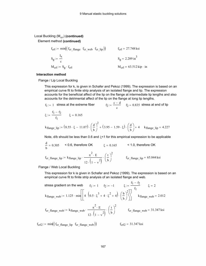
9 Manual elastic buckling solutions
< 0.6, therefore OK ξ 0.165= < 1.0, therefore OK
fcr_flange_lip kflange_lipπ
2E⋅
12 1 ν2
−( )⋅
⋅tb
2⋅:= fcr_flange_lip 65.844 ksi=
Flange / Web Local Buckling
This expression for k is given in Schafer and Pekoz (1999). The expression is based on an empirical curve fit to finite strip analysis of an isolated flange and web.
stress gradient on the web f1 1:= f2 1−:= ξf1 f2−
f1:= ξ 2=
kflange_web 1.125 min 4 0.5 ξ3
⋅ 4 ξ2
⋅+ 4+( ) bh
2⋅
⋅:= kflange_web 2.012=
fcr_flange_web kflange_webπ
2E⋅
12 1 ν2
−( )⋅
⋅tb
2⋅:= fcr_flange_web 31.347 ksi=
fcrl2 min fcr_flange_lip fcr_flange_web( )( ):= fcrl2 31.347 ksi=
Local Buckling (Mcrl) (continued) Element method (continued)
fcrl min fcr_flange fcr_web fcr_lip( )( ):= fcrl 27.748 ksi=
SgIxc
:= Sg 2.289 in3=
Mcrl Sg fcrl⋅:= Mcrl 63.512 kip in⋅=
Interaction method
Flange / Lip Local Buckling
This expression for k, is given in Schafer and Pekoz (1999). The expression is based on an empirical curve fit to finite strip analysis of an isolated flange and lip. The expression accounts for the beneficial affect of the lip on the flange at intermediate lip lengths and also accounts for the detrimental affect of the lip on the flange at long lip lengths.
f1 1:= stress at the extreme fiber f2c d−
c:= f2 0.835= stress at end of lip
ξf1 f2−
f1:= ξ 0.165=
kflange_lip 8.55 ξ⋅ 11.07−( ) db
2⋅ 3.95 1.59 ξ⋅−( ) d
b
⋅+ 4+:= kflange_lip 4.227=
Note, d/b should be less than 0.6 and ξ<1 for this empirical expression to be applicable
db
0.305=
167

9 Manual elastic buckling solutions
fcrdkφfe kφwe+
kφfg kφwg+:=
Determine the distortional buckling stress:
kφwg 1.783 10 3−× in2
=
kφwgh t⋅ π
2⋅
13440
45360 ψ⋅ 62160+( ) Lcr
h
2
⋅ 448 π2
⋅+h
Lcr
253 3 ψ⋅+( )⋅ π
4⋅+
π4
28 π2
⋅Lcr
h
2
⋅+ 420Lcr
h
4
⋅+
⋅:=
ψ 1−=ψf1f2
:=f2 1−:=f1 1:=stress gradient on the web (note ψ=1-ξ and ξ was used in the earlier stress gradient definitions)
kφwe 0.21 kip=kφweE t3⋅
12 1 ν2
−( )⋅
3h
π
Lcr
219 h⋅
60⋅+
π
Lcr
4h3
240⋅+
⋅:=
Determine the elastic and "geometric" rotational spring stiffness of the web:
kφfg 8.658 10 3−× in2
=
kφfgπ
Lcr
2Af xof hxf−( )2
Ixyf
Iyf
2
⋅ 2 yof⋅ xof hxf−( )⋅Ixyf
Iyf
⋅− hxf
2+ yof
2+
⋅ Ixf+ Iyf+
⋅:=
kφfe 0.223 kip=
kφfeπ
Lcr
4E Ixf⋅ xof hxf−( )2⋅ E Cwf⋅+ E
Ixyf2
Iyf⋅ xof hxf−( )2⋅−
⋅π
Lcr
2G⋅ Jf⋅+:=
Determine the elastic and "geometric" rotational spring stiffness of the flange:
If bracing is provided that restricts the distortional mode at some length less thanLcr, then this length should be used in place of Lcr.
Lcr 25.783 in=Lcr4 π
4⋅ h⋅ 1 ν
2−( )⋅
t3Ixf xof hxf−( )2⋅ Cwf+
Ixyf2
Iyfxof hxf−( )2⋅−
⋅π
4h4⋅
720+
1
4
:=
Determine the critical half-wavelength at which distortional buckling occurs:
Distortional Buckling (Mcrd)
In this example local buckling is controlled by the slender web, but including the web/flange interaction is important as it increases the predicted buckling stress by 13%.
Mcrl2 71.75 kip in⋅=Mcrl2 Sg fcrl2⋅:=
168

9 Manual elastic buckling solutions
Mcre 57.291 kip in⋅=Mcre Sg Fcre⋅:=
note, for singly symmetric sections the x-axis is assumed to be the axis of symmetry
(Eq. C3.1.2.1-5)Fe 26.064 ksi=FeCb ro⋅ A⋅
Sgσey σ t⋅⋅:=
lateral-torsional buckling per C3.1.2.1(a)
(Eq. C3.1.2.1-9)σ t 18.783 ksi=σ t1
A ro2
⋅G J⋅
π2
E⋅ Cw⋅
Kt Lt⋅( )2+
⋅:=
(Eq. C3.1.2.1-8)σey 16.019 ksi=σeyπ
2E⋅
Ky Ly⋅
ry
2:=
individual buckling modes, per C3.1.2.1(a)
Lt 10 ft⋅:=Ly 10 ft⋅:=
(simplification of C3.1.2.1-10)Cb 1:=Kt 1:=Ky 1:=
Length and bracing conditions (for example...)
Global cross-section properties are given for this section in AISI Design Manual (2002), Example I-1: C-Section With Lips - Gross Section Properties and are listed above under column: global buckling
Global buckling (Mcre)
Mcrd 94.784 kip in⋅=Mcrd Sg fcrd⋅:=
fcrd 41.41 ksi=
169
170
10 References
AISI (2001) North American Specification for the Design of Cold-Formed Steel Structural Members. American Iron and Steel Institute, Washington, D.C., AISI/COS/NASPEC 2001
AISI (2002) AISI Manual of Cold-Formed Steel Design. American Iron and Steel Institute, Washington, D.C.
AISI (2004) Supplement 2004 to the North American Specification for the Design of Cold-Formed Steel Structural Members, 2001 Edition: Appendix 1, Design of Cold-Formed Steel Structural Members Using Direct Strength Method. American Iron and Steel Institute, Washington, D.C., SG05-1.
AISI (2004b) Standard for Cold-Formed Steel Framing – Wall Stud Design. American Iron and Steel Institute. Washington, DC. AISI/COFS/WSD-2004.
Allen, H.G., Bulson, P.S. (1980). Background to Buckling. McGraw-Hill. Cheung, Y.K., Tham, L.G. (1998). The Finite Strip Method. CRC Press. Galambos, T.V. (1998). Guide to Stability Design Criteria for Metal Structures. 5th Ed. Wiley. Hancock, G.J., Murray, T.M., Ellifritt, D.S. (2001) Cold-Formed Steel Structures to the AISI
Specification. Marcel Dekker. 398 pp. Sarawit, T.P. (2003). Cold-Formed Steel Frame and Beam-Column Design. Ph.D. Dissertation.
Cornell University, Ithaca, NY. Schafer, B.W. (1997). Cold-Formed Steel Behavior and Design: Analytical and Numerical
Modeling. Ph.D. Thesis. Cornell University, Ithaca, NY. of Elements and Members with Longitudinal Stiffeners.” ASCE, Journal of Structural
Engineering. 128 (3) 289-299. Schafer, B.W. (2002). “Local, Distortional, and Euler Buckling in Thin-walled Columns.”
ASCE, Journal of Structural Engineering. 128 (3) 289-299. Schafer, B.W. (2005) CUFSM: Elastic Buckling Analysis of thin-walled members by the finite
strip method. (Open Source Software) www.ce.jhu.edu/bschafer/cufsm Schafer, B.W., Ádány, S. (2005). “Understanding and classifying local, distortional and global
buckling in open thin-walled members.” Annual Technical Session and Meeting, Structural Stability Research Council, May, 2005. Montreal, Quebec, Canada.
Schafer, B.W., Peköz, T. (1998). “Cold-Formed Steel Members with Multiple Longitudinal Intermediate Stiffeners in the Compression Flange.” ASCE, Journal of Structural Engineering. 124 (10) 1175-1181.
Shahwan, K.W., Waas, A.M. (1998). “Buckling of Unilaterally Constrained Infinite Plates.” ASCE. Journal of Engineering Mechanics. 124 (2) 127-236
Silvestre, N., Camotim, D. (2004). “Distortional buckling formulae for cold-formed steel C and Z-section members: Part I – Derivation.” Elsevier, Thin-Walled Structures. 42 (11) 1567-1597
Timoshenko, S.P., Gere, J.M. (1961). Theory of Elastic Stability. 2nd Ed. McGraw Hill.
171
Yu, C. (2005). Distortional Buckling of Cold-Formed Steel Members in Bending. Ph.D. Dissertation, Johns Hopkins University, Baltimore, MD.