Embed Size (px)
Citation preview

DIRECT USE OF PGV FOR ESTIMATING PEAK NONLINEAR OSCILLATOR DISPLACEMENTS
A THESIS SUBMITTED TO THE GRADUATE SCHOOL OF NATURAL AND APPLIED SCIENCES
OF MIDDLE EAST TECHNICAL UNIVERSITY
BY
BİLGE KÜÇÜKDOĞAN
IN PARTIAL FULFILLMENT OF THE REQUIREMENTS FOR
THE DEGREE OF MASTER OF SCIENCE IN
CIVIL ENGINEERING
NOVEMBER 2007

Approval of the Thesis;
DIRECT USE OF PGV FOR ESTIMATING PEAK NONLINEAR
OSCILLATOR DISPLACEMENTS
Submitted by BİLGE KÜÇÜKDOĞAN in partial fulfillment of the requirements for the degree of Master of Science in Civil Engineering, Middle East Technical University by, Prof. Dr. Canan Özgen Dean, Graduate School of Natural and Applied Sciences
Prof. Dr. Güney Özcebe Head of Department, Dept. of Civil Engineering Assoc. Prof. Dr. Sinan Dede Akkar Supervisor, Dept. of Civil Engineering, METU Examining Committee Members: Prof. Dr. Polat Gülkan (*) Civil Engineering Dept., METU Assoc. Prof. Dr. Sinan Dede Akkar (**) Civil Engineering Dept., METU Prof. Dr. Haluk Sucuoğlu Civil Engineering Dept., METU Assoc. Prof. Dr. Ahmet Yakut Civil Engineering Dept., METU Assist. Prof. Dr. Tolga Yılmaz Engineering Sciene Dept., METU
Date:
(*) Head of Examining Committee
(**) Supervisor

iii
PLAGIARISM
I hereby declare that all information in this document has been obtained
and presented in accordance with academic rules and ethical conduct. I
also declare that, as required by these rules and conduct, I have fully
cited and referenced all material and results that are not original to this
work.
Name, Last name : Bilge Küçükdoğan
Signature :

iv
ABSTRACT
DIRECT USE OF PGV FOR ESTIMATING PEAK NONLINEAR OSCILLATOR DISPLACEMENTS
KÜÇÜKDOĞAN, Bilge
M.S., Department of Civil Engineering
Supervisor: Assoc. Prof. Dr. Sinan AKKAR
Co-supervisor : Prof. Dr. M. Semih YÜCEMEN
November 2007, 129 pages
Recently established approximate methods for estimating the lateral
deformation demands on structures are based on the prediction of
nonlinear oscillator displacements (Sd,ie). In this study, a predictive
model is proposed to estimate the inelastic spectral displacement as a
function of peak ground velocity (PGV). Prior to the generation of the
proposed model, nonlinear response history analysis is conducted on
several building models of wide fundamental period range and
hysteretic behavior to observe the performance of selected demands
and the chosen ground-motion intensity measures (peak ground
acceleration, PGA, peak ground velocity, PGV and elastic pseudo
spectral acceleration at the fundamental period (PSa(T1)). Confined to
v
the building models used and ground motion dataset, the correlation
studies revealed the superiority of PGV with respect to the other
intensity measures while identifying the variation in global deformation
demands of structural systems (i.e., maximum roof and maximum
interstory drift ratio). This rational is the deriving force for proposing the
PGV based prediction model. The proposed model accounts for the
variation of Sd,ie for bilinear hysteretic behavior under constant ductility
(µ) and normalized strength ratio (R) associated with postyield stiffness
ratios of α= 0% and α= 5%. Confined to the limitations imposed by the
ground-motion database, the predictive model can estimate Sd,ie by
employing the PGV predictions obtained from the attenuation
relationships. This way the influence of important seismological
parameters can be incorporated to the variation of Sd,ie in a fairly
rationale manner. Various case studies are presented to show the
consistent estimations of Sd,ie by the proposed model using the PGV
values obtained from recent ground motion prediction equations.
Keywords: Peak ground velocity; Inelastic spectral displacement;
Ground-motion predictive models; Regression; Seismic design/
performance assessment

vi
ÖZ
DOĞRUSAL OLMAYAN MAKSİMUM TEK DERECELİ SİSTEM
DEPLASMANI TAHMİNİNDE MAKSİMUM YER HAREKETİ HIZININ
KULLANILMASI
KÜÇÜKDOĞAN, Bilge
Yüksek Lisans, İnşaat Mühendisliği Bölümü
Tez Yöneticisi : Doç. Dr. Sinan AKKAR
Yardımcı Tez Yöneticisi : Prof. Dr. M. Semih YÜCEMEN
Kasım 2007, 129 sayfa
Bina sistemleri için yanal deformasyon taleplerini yaklaşık olarak tahmin
eden metodların pek çoğu doğrusal olmayan tek dereceli sistem
(osilatör) maksimum deplasmanlarını (Sd,ie) temel almaktadır. Bu
çalışmada, doğrusal olmayan spektral deplasmanları maksimum yer
hareketi hızının (MYH) bir fonksiyonu olarak hesaplayan bir model
önerilmiştir. Modelin önerilmesinden önce, seçilen yer hareketi şiddet
parametrelerinin (maksimum yer ivmesi (MYİ), maksimum yer hareketi
hızı (MYH) ve temel periyottaki elastik spektral ivme (PSa(T1)) ile global
deformasyon talepleri arasındaki ilişkiyi gözlemlemek üzere, geniş bir
bantta değişim gösteren temel periyot ve histeretik davranım
özelliklerine sahip bir grup çok serbestlik dereceli model elastik olmayan
zaman mukabele hesaplarına tabii tutulmuştur. Global deformasyon

vii
talepleri ile (maksimum kat arası ötelemesi ve maksimum deformasyon)
yer hareketi şiddet parametreleri arasında yapılan korelasyon
çalışmaları sonucunda MYH parametresinin diğer yer hareketi
parametrelerine nazaran bina global deformasyon taleplerin ile daha
uyumlu olduğu görülmüş ve önerilen model bu rasyonel ışığında
geliştirilmiştir. Önerilen model, ve sabit süneklik (µ) ve normalize edilmiş
mukavemet oranları (R) için doğrusal olmayan spektral deplasman
değişimlerini akma sonrası yanal rijitlik oranı (α) α= %0 ve α= %5 çift
doğrulu histeretik model için gösterebilmektedir. Seçilen yer hareketi
veritabanının özelliklerine bağlı olarak, Sd,ie değerlerini yer hareketi MYH
değerlerine bağlı kalarak hesaplayabilmektedir. Böylelikle, model
önemli sismolojik parametrelerin Sd,ie üzerindeki etkisini de
yansıtabilmektedir. Modelin yakın zamanlarda geliştirilen yer hareketi
tahmin denklemlerinden elde edilmiş MYH değerleri kullanılarak Sd,ie için
tutarlı tahminler yaptığı çeşitli örneklerle gösterilmiştir.
Anahtar Kelimeler : Maksimum yer hareketi hızı; Elastik olmayan
spektral deplasman; Yer hareketi tahmin modelleri; Regresyon; Sismik
tasarım/performans değerlendirmesi

viii
To,
Doç.Dr. Sinan D. AKKAR

ix
ACKNOWLEDGEMENT
“Do something everyday that you don't want to do; this is the golden rule for acquiring the habit of doing
your duty without pain.”
Mark Twain
“Was ihn nicht umbringt, macht ihn stärker.”
Friedrich Wilhelm Nietzsche
This study is particulary helpful to clearly define my interests and
desires and a milestone only during which I was able to decide on the
subject and the career that I want to pursue for the future. It is a
pleasure to thank the many people who made this thesis possible.
It is difficult to overstate my gratitude to my supervisor, Assoc.Prof. Dr.
Sinan Akkar, to whom I dedicated this study. Mr. Akkar, in every single
stage of the work, has also been abundantly helpful, and has assisted
me in numerous ways, including providing me the necessary articles
and program codes to proceed the analyses, introducing patiently new
softwares with a great effort to explain things clearly and simply.
This work would not have been possible without the support and
encouragement of Erhan Karaesmen and Engin Karaesmen who have
always been near me opening new perspectives in my mind and
believing in me. Knowing this family has been the most precious gain
that I had during my years in Middle East Technical University.
I would like to thank Assist.Prof. Dr Tolga Yılmaz, for his guidance in
regression analysis and statistical evaluation of the results. I have also
to thank my examinıng committee members for their invaluable advices
and suggestions that improved the study considerably.

x
I offer my sincere thanks to: my beloved family my mother Emel
Küçükdogan, my grandfather Adem Hablemitoglu, my sister İdil Belgin
Küçükdogan and my dear aunt Efser Koçakoglu for their unique love
and support throughout my life and their endless faith in me; my father
Alaettin Küçükdoğan and my uncle Necip Hablemitoğlu for their
determination of pursuing their believes even confronting the death
without slightest hesitation and fear.
Sincere thanks to all my friends whom I found beside me whenever I
needed and felt blue for their refreshing energy, their encouraging and
calming words and their love. Many thanks to:
Chorists of J.S.Bach Choir: Duygu, Özgür, Gökçen, Derya, Öncü, Esra,
Güçlü, Moldiyar, Janar, Hamdi, Can, Bülent and many others for their
absolutely limitless joy and energy; The members of the Arinna Sailing
Team, Tayfun, Serhan, Koray, Oguz and Semih for their willingness to
share the mystery of the eternal blue with me; Tayfun Hız for offering
me a big barrel of wine upon the completion of this study; Utku Kartal,
for his sincere friendship and sense of humor; Semih Demirer, for his
courage, emotional support and mostly for his patience to calm me
down; Bekir Özer Ay, Sami Demiroluk, Zerrin Ardıç Eminağa, Hazım
Yılmaz, for their friendship and their support during every stages of the
study; Özge Göbelez, for being the indispensable company at the times
when the things all went wrong; Tuba Eroğlu for her courage, her help
in technical matters; Vanessa Rheinheimer for her understanding and
feeding me for the last week before the exam.
Finally, and most importantly, I am profoundly grateful to Mustafa Kemal
Atatürk. I owe him my being able to write this MS dissertation as a
woman while other women in other parts of the world still fight for their
gender rights.

xi
TABLE OF CONTENTS
ABSTRACT......................................................................................... iv
ÖZ........................................................................................................ vi
ACKNOWLEDGEMENT...................................................................... ix
TABLE OF CONTENTS ...................................................................... xi
LIST OF FIGURES............................................................................ xiv
LIST OF TABLES.............................................................................. xix
CHAPTER
1. INTRODUCTION .................................................................. 1
1.1 General ........................................................................ 1
1.2 Previous Research....................................................... 3
1.3 Disposition of the Study ............................................... 7
2. GROUND MOTIONS AND MDOF ANALYSES ................... 9
2.1 Description of Ground Motions..................................... 9
2.2 Building models used for the first ground motion
database..................................................................... 17
2.3 Nonlinear Response History Analyses of the Frame
Models Using First Ground-motion Dataset................ 21
3. ESTIMATION OF INELASTIC SPECTRAL
DISPLACEMENTS AS A FUNCTION OF PEAK GROUND
VELOCITY.......................................................................... 36
3.1 Introduction ................................................................ 36
3.2 Regression Analyses ................................................. 36
3.3 Simplified Expressions for Standard Deviations......... 64

xii
3.4 Application of the Proposed Model ............................ 66
4. CONCLUDING REMARKS ................................................ 74
4.1 General ...................................................................... 74
4.2 Summary and Conclusions of Chapter 2.................... 75
4.3 Summary and Conclusions of Chapter 3.................... 77
4.4 Recommendation for Future Studies ......................... 79
REFERENCES ................................................................................... 81
APPENDIX ......................................................................................... 88
A. MDOF MODELS................................................................. 88
A.1 General...................................................................... 88
A.2 Model 3e1.................................................................. 91
A.3 Model 3e2.................................................................. 91
A.4 Model 3e3.................................................................. 92
A.5 Model 3e1’ ................................................................. 92
A.6 Model 3e2’ ................................................................. 93
A.7 Model 5e1.................................................................. 94
A.8 Model 5e2.................................................................. 95
A.9 Model 5e3.................................................................. 96
A.10 Model 5e1’ ............................................................... 97
A.11 Model 5e2’ ............................................................... 98
A.12 Model 7e1................................................................ 99
A.13 Model 7e2.............................................................. 100
A.14 Model 7e3.............................................................. 101
A.15 Model 7e1’ ............................................................. 102

xiii
A.16 Model 7e2’ ............................................................. 103
A.17 Model 9e1.............................................................. 104
A.18 Model 9e2.............................................................. 105
A.19 Model 9e3.............................................................. 106
A.20 Model 9e1’ ............................................................. 107
A.21 Model 9e2’ ............................................................. 108
B. RELEVANT TABLES AND FIGURES OF CHAPTER 2 .. 109
B.1 Dynamic Properties of the Models........................... 109
B.2 Pushover Curves and ADRS of Models................... 110
C. PREDICTION EQUATIONS FOR GROUND MOTIONS AND
ELASTIC SPECTRAL DISPLACEMENT......................... 126
C.1 Prediction equation for ground motion (Akkar and
Bommer)................................................................... 126
C.2 Prediction equation for ground motion (Boore and
Atkinson)................................................................... 127
C.3 Prediction equation for elastic spectral displacement
(Akkar and Bommer) ................................................ 129

xiv
LIST OF FIGURES
FIGURES PAGE
Figure 2.1 Magnitude distance, PGV range and magnitude range
distribution of the ground motion dataset 1. .................. 14
Figure 2.2 Magnitude distance, PGV range and magnitude range
distribution of the ground motion dataset 2 ................... 15
Figure 2.3 Median response and smoothed design spectra of the
ground-motions assembled from the first ground-motion
dataset ......................................................................... 18
Figure 2.4 Typical sketch of 9 story analytical model...................... 21
Figure 2.5 Variation of MRDR with PGA, PGV and PSa(T1) for
nondegrading building models ...................................... 27
Figure 2.6 Variation of MIDR with PGA, PGV and PSa(T1) for
nondegrading building models. ..................................... 28
Figure 2.7 Variation of MRDR with PGA, PGV and PSa(T1) for
stiffness degrading building models. ............................. 29
Figure 2.8 Variation of MIDR with PGA, PGV and PSa(T1) for
stiffness degrading building models. ............................. 30
Figure 2.9 Variation of MRDR with PGA, PGV and PSa(T1) for
stiffness and strength degrading building models.......... 31
Figure 2.10 Variation of MIDR with PGA, PGV and PSa(T1) for
stiffness and strength degrading building models.......... 32
Figure 2.11 Comparison of the Spearman’s correlation coefficient
values of ground motion intensityl demand measures... 33

xv
Figure 3.1 Influence of certain ground-motion parameters on
Sd,e/(PGV×T) ................................................................. 39
Figure 3.2 The variation of regression coefficients (b0,b1 and b2) as a
function of period for constant ductility .......................... 47
Figure 3.3 The variation of regression coefficients (b0,b1 and b2) as a
function of period for normalized lateral strength .......... 48
Figure 3.4 Normal probability plots of the residueals at µ and R
equal to 4 for T=0.5, 1.0, 1.5 and 2.0 α = 0 %............... 50
Figure 3.5 Normal probability plots of the residueals at µ and R
equal to 4 for T=0.5, 1.0, 1.5 and 2.0 when α = 5 % ..... 51
Figure 3.6 Residual plots as a function of M for µ =6 and R=6 at
T=0.5, 1.0, 1.5 and 2.0 when α=0% ............................. 53
Figure 3.7 Residual plots in terms of dependent parameter for
distinct µ and R values considering the entire database54
Figure 3.8 The dependent parameter vs magnitude plots with the
estimation of predictive model for different R values when
α = 0 % (T=0.5s) ........................................................... 56
Figure 3.9 The dependent parameter vs magnitude plots with the
estimation of predictive model for different R values when
α = 5 % (T=0.5s) ........................................................... 57
Figure 3.10 The dependent parameter vs magnitude plots with the
estimation of predictive model for different R values when
α = 0 % (T=2.0s) ........................................................... 58
Figure 3.11 The dependent parameter vs magnitude plots with the
estimation of predictive model for different R values when
α = 5 % (T=2.0s) ........................................................... 59
Figure 3.12 The dependent parameter vs magnitude plots with the
estimation of predictive model for different µ values when
α = 0 % (T=0.5s) ........................................................... 60

xvi
Figure 3.13 The dependent parameter vs magnitude plots with the
estimation of predictive model for different µ values when
α = 5 % (T=0.5s) ........................................................... 61
Figure 3.14 The dependent parameter vs magnitude plots with the
estimation of predictive model for different µ values when
α = 0 % (T=2.0s) ........................................................... 62
Figure 3.15 The dependent parameter vs magnitude plots with the
estimation of predictive model for different µ values when
α = 5 % (T=2.0s) ........................................................... 63
Figure 3.16 Smooth variation of standard deviations........................ 66
Figure 3.17 Inelastic spectral displacement estimations of the
proposed predictive model for constant µ and constant R
as a function of magnitude when α=0% ........................ 70
Figure 3.18 Inelastic spectral displacement estimations of the
proposed predictive model for constant µ and constant R
as a function of magnitude when α=5% ........................ 71
Figure 3.19 Influence of PGV variation as a function of distance on
inelastic spectral displacement estimations for constant
ductility and for constant strength.................................. 72
Figure A.1 Stress-straing curve of concrete.................................... 89
Figure A.2 Stress-straing curve of steel .......................................... 89
Figure A.3 Confinement effectiveness ............................................ 90
Figure A.4 Reinforcement areas in cm2 for 3e1 .............................. 91
Figure A.5 Reinforcement areas in cm2 for 3e2 .............................. 91
Figure A.6 Reinforcement areas in cm2 for 3e3 .............................. 92
Figure A.7 Reinforcement areas in cm2 for 3e1’.............................. 92
Figure A.8 Reinforcement areas in cm2 for 3e2’.............................. 93
Figure A.9 Reinforcement areas in cm2 for 5e1 .............................. 94
Figure A.10 Reinforcement areas in cm2 for 5e2 .............................. 95
Figure A.11 Reinforcement areas in cm2 for 5e3 .............................. 96
Figure A.12 Reinforcement areas in cm2 for 5e1’.............................. 97

xvii
Figure A.13 Reinforcement areas in cm2 for 5e2’.............................. 98
Figure A.14 Reinforcement areas in cm2 for 7e1 .............................. 99
Figure A.15 Reinforcement areas in cm2 for 7e2 ............................ 100
Figure A.16 Reinforcement areas in cm2 for 7e3 ............................ 101
Figure A.17 Reinforcement areas in cm2 for 7e1’............................ 102
Figure A.18 Reinforcement areas in cm2 for 7e2’............................ 103
Figure A.19 Reinforcement areas in cm2 for 9e1 ............................ 104
Figure A.20 Reinforcement areas in cm2 for 9e2 ............................ 105
Figure A.21 Reinforcement areas in cm2 for 9e3 ............................ 106
Figure A.22 Reinforcement areas in cm2 for 9e1’............................ 107
Figure A.23 Reinforcement areas in cm2 for 9e2’............................ 108
Figure B.1 Pushover curves and ADRS of e1 models for
nondegrading case...................................................... 110
Figure B.2 Pushover curves and ADRS of e2 models for
nondegrading case...................................................... 111
Figure B.3 Pushover curves and ADRS of e3 models for
nondegrading case...................................................... 112
Figure B.4 Pushover curves and ADRS of e1’ models for
nondegrading case...................................................... 113
Figure B.5 Pushover curves and ADRS of e2’ models for
nondegrading case...................................................... 114
Figure B.6 Pushover curves and ADRS of e1 models for stiffness
degrading case............................................................ 115
Figure B.7 Pushover curves and ADRS of e2 models for stiffness
degrading case............................................................ 116
Figure B.8 Pushover curves and ADRS of e3 models for stiffness
degrading case............................................................ 117
Figure B.9 Pushover curves and ADRS of e1’ models for stiffness
degrading case............................................................ 118
Figure B.10 Pushover curves and ADRS of e2’ models for stiffness
degrading case............................................................ 119

xviii
Figure B.11 Pushover curves and ADRS of e1 models for stiffness
and strength degrading case....................................... 120
Figure B.12 Pushover curves and ADRS of e2 models for stiffness
and strength degrading case....................................... 121
Figure B.13 Pushover curves and ADRS of e3 models for stiffness
and strength degrading case....................................... 122
Figure B.14 Pushover curves and ADRS of e1’ models for stiffness
and strength degrading case....................................... 123
Figure B.15 Pushover curves and ADRS of e2’ models for stiffness
and strength degrading case....................................... 124

xix
LIST OF TABLES
TABLE PAGE
Table 2.1 Bin 1 of the first ground-motion data set. ....................... 11
Table 2.2 Bin 2 of the first ground-motion data set. ....................... 12
Table 2.3 Bin 3 of the first ground-motion data set. ....................... 13
Table 2.4 Important seismological features of suite of ground
motion records ............................................................ 16
Table 2.5 Different properties of models ........................................ 20
Table 2.6 Response history analyses conducted in the study ....... 23
Table 2.7 Hysteretic model parameters used in the analyses........ 24
Table 2.8 Spearman’s coefficient values between intensity
measures and global demand parameters under three
different structural behavior ........................................... 33
Table 3.1 Regression coefficients for constant µ peak inelastic
oscillator displacements when α = 0% .......................... 42
Table 3.2 Regression coefficients for constant µ peak inelastic
oscillator displacements when α = 5% .......................... 43
Table 3.3 Regression coefficients for constant R peak inelastic
oscillator displacements when α = 0% .......................... 44
Table 3.4 Regression coefficients for constant R peak inelastic
oscillator displacements when α = 5% .......................... 45
Table 3.5 R2 values of bilinear curve fit on mean magnitude and the
predicted parameter values........................................... 64
Table A.1 Distances values used in the design of members ......... 90
Table B.1 Dynamic properties of e1, e2, e3, e1’ and e2’ models. 109
Table B.2 Idealized pushover curve parameters.......................... 125
Table C.1 Regression coefficients of the prediction equation ...... 125
1
CHAPTER 1
INTRODUCTION
1.1 General
Performance based approach in the field of earthquake engineering
aims to envisage the performance of a structure under common or
extreme loads with a quantifiable confidence responding the needs of
users and society (Krawinkler, 1999). The key point in the performance
assessment studies is the estimation of lateral deformation demands in
buildings under seismic excitation. Seismic excitation is quantified
through a ground-motion intensity measure (IM) while deformation
demand is depicted in terms of demand measure (DM). The disposition
of the intricate relationship between IM and DM has been the eventual
aim of the studies in this field. Several different methods are employed
to achieve this objective with a wide spectrum of complexity, accuracy
and computational effort features. Among those, response history
analyses, albeit give more accurate results, are demanding in input
preparation, modeling and data evaluation processes which makes the
approach impractical especially beyond the elastic capacity (Metin,
2006; Ruiz-Garcia and Miranda, 2006; Yılmaz, 2007). Therefore, a
great deal of effort has been devoted by the researchers to simplify the
procedures on the estimation of nonlinear deformation demands on
structures. Various recommendations have been proposed and
academic studies have been conducted for the evaluation and
rehabilitation of existing structures by professional academic agencies
and establishments that introduce simplified analysis methods based on
the maximum displacements of single-degree-of-freedom-systems

2
(SDOF) (e.g. ATC-40 (ATC,1996); FEMA 273/274 (ATC, 1997); FEMA-
356 (ASCE, 2000) ; Miranda, 1999; Miranda and Garcia, 2002; Farrow
and Kurama, 2004).
The performance assessment studies have utilized a variety of ground
motion parameters as intensity measures which, in a way, portray the
fundamental features of the ground motion as amplitude, frequency
content and duration (Kramer, 1996). Two ground acceleration related
parameters peak ground acceleration (PGA) and pseudo spectral
acceleration at the fundamental period (PSa(T1)) have been widely
preferred among the several ground motion intensity parameters
defined in the literature. Douglas (2003) concludes that this common
use is due to the predominance of many earthquake resistant design
methods that are based on the response spectrum of acceleration.
There exist several prediction equations which promote PGA and
PSa(T1) as well-recognized IMs. On the other hand, although the
relative scarcity of prediction equations for PGV, many researches have
been conducted to scrutinize and reveal the properties of PGV and its
adequacy as an intensity measure in the last decade details of which
will be discussed in the succeeding section.
The main subject of this study is to propose a predictive model to
estimate the peak oscillator displacements as a function of PGV for
bilinear hysteretic behavior under constant ductility (µ) and normalized
lateral strength ratios (R) associated with α= 0% and α= 5% post yield
stiffness ratio with independent variables, magnitude (M) and period (T),
respectively. The secondary objective is to observe the correlation
between intensity measures (PGA, PGV and PSa(T1) and global
demand measures (MIDR and MRDR) in multi-degree of freedom
systems as a result of which PGV is selected as the ground motion
intensity parameter for the predictive model. As a part of the thesis, the

3
use of predictive model with ground motion prediction equations of
Akkar and Bommer (2007a, 2007b) is presented. The study has made
use of 60 ground motions in the MDOF analyses and 109 ground-
motions in the regression study of the predictive model, 20 model
frames with 3-to 9-story levels to achieve these objectives.
1.2 Previous Research
In the estimation of the expected peak inelastic oscillator displacements
(inelastic spectral displacement, Sd,ie), approximate models have made
use of elastic period (T) dependent empirical relationships for a given
displacement ductility (µ) or normalized lateral strength (R). Studies
conducted by Velestos and Newmark (1960) and Newmark and Hall
(1973, 1982) have been the pioneer studies that are based on Rµ - µ - T
relationships within the context of force-based design to approximate
the oscillator yield-strength (Fy) that would limit a predefined µ value.
During the following decades many useful period-dependent empirical
regression equations for direct estimation of Sd,ie as a function of R
(Ruiz-García and Miranda, 2003; Chopra and Chintanapakdee, 2004)
or µ (e.g. Miranda, 2000; MacRae and Tagava, 2002; Chopra and
Chintanapakdee, 2004; Ruiz-García and Miranda, 2004) have been
proposed. These studies used ground motion datasets to establish the
empirical relationships based on the quantity and quality of
accumulated strong-motion records at the time when they were
conducted. Different features of ground motion parameters have been
stood out depending on the objective of the study. For the definition of
ground-motion frequency content, the studies that followed the Velestos
and Newmark approach have made use of peak ground motion values.
They then derived their empirical relationships to relate elastic to
inelastic oscillator response for the spectral period ranges described by
the peak ground motion ratios. In these studies datasets were classified

4
according to ground-motion duration, moderate- to large-magnitude
events, pulse-dominant signals or severe events produced by a
particular fault type (e.g. Vidic et al., 1994; Cuesta et al., 2003; Riddell
et al., 2002). The studies conducted by Elghadamsi and Mohraz (1987),
Sewel (1989), Nassar and Krawinkler (1991), Miranda (1993, 2000),
Ruiz-García and Miranda (2003, 2004), Arroyo and Teran (2003) mostly
emphasized the influence of different site classes on the estimation of
Sd,ie using small- to large-size ground-motion datasets. Different
magnitude-distance bins as well as different site classes were used for
ground motions in the studies of Chopra and Chintanapakdee (2003,
2004). Researchers such as MacRae and Roeder (1999), Baéz and
Miranda (2000), MacRae et al. (2001) and Chopra and Chintanapakdee
(2001) shaped their Sd,ie predictive expressions on the differences
between near- and far-fault ground-motion records. These studies
revealed significant insight about the nonlinear oscillator behavior under
different load-deformation rules. The studies by Miranda and Bertero
(1994) and Mahin and Bertero (1981) may also be referred for a
detailed review on nonlinear oscillator response studies for the
estimation of Sd,ie.
Regardless of the approximate model proposed, the major concept
used in the estimation of Sd,ie is
eaedied PST
RS
RS ,
2
,,2
==
π
µµ (1.1)
In the case of Rµ - µ - T relations, Sd,ie can be estimated using the
expected Rµ for a given µ - T pair from its elastic counterpart Sd,e (or
equivalently utilizing elastic pseudo-spectral acceleration, PSa,e that can
be related to Sd,e through the constant (T/2π)2 as shown in Eq. (1.1)).
For the direct empirical relationships, Sd,ie is related to Sd,e by using the

5
regression equations that mimic the expected variation of µ/R either for
a constant ductility level or normalized lateral strength ratio with the
inclusion of a period-dependent modification factor (Cx) either for
constant µ or for constant R. Thus, an alternative way of expressing Eq.
(1.1) is given below
eaxedxied PST
CSCS ,
2
,,2
==
π (2)
The expressions presented in Eqs. (1.1) and (1.2) establish a linear
relationship between inelastic and elastic spectral displacements (or
equivalently a linear variation between Sd,ie and Sa,e) for a given elastic
period, T. As a matter of fact this approach is one of the current
methods used in the simplified nonlinear static procedures (e.g., FEMA,
1997; ASCE, 2000; FEMA, 2003; ATC, 2005). Note that the ongoing
research efforts for the estimation of Sd,ie continuously result in new
predictive models. In a recent study, Tothong and Cornell (2006)
proposed an attenuation relationship for estimating Sd,ie as a function of
oscillator yield-strength and magnitude.
The attention received by peak ground velocity (PGV) in the technical
literature is much less than that of peak ground acceleration and
spectral ordinates (Bommer and Alarcón, 2006). However, PGV has
various applications in earthquake engineering field as a damage
potential indicator of ground motion to structural damage. The study of
Wu et al (1999) revealed that PGV correlates better than PGA with
Modified Mercalli Intensity (MMI) for higher values of intensity. The
similar results were observed from the derived relationships of Kaka
and Atkinson (2004) that estimated MMI from PGV for eastern North
America. In their study that focused on the damage potential of
earthquake ground motions based on inelastic dynamic response of

6
equivalent single degree of freedom structures, Sucuoğlu et al (1999)
concluded that PGV is a promising seismic hazard parameter.
Researchers like Miyakoshi et al (1998) and Yamazaki and Murao
(2000) used PGV to derive vulnerability functions using the damage
data from the 1995 Hyogo-ken Nanbu earthquake in Japan. PGV was
used as a parameter that measures the potential of earthquake ground
motions to cause damage in structures of intermediate periods of
vibration by Fajfar et al (1990). A more recent study conducted by Akkar
and Özen (2005) investigated the effect of peak ground velocity on
deformation demands for SDOF systems using 60 near fault records of
moderate to large magnitude. The correlations of PGV, PGA, spectral
acceleration (Sa) and PGV/PGA as intensity measures with inelastic
deformation demands of oscillators were compared between the period
range of 0 to 4 seconds and the results revealed that PGV correlates
better than the other intensity measures. The authors suggested PGV
“as a stable candidate for ground motion intensity measure in simplified
seismic assessment methods”. As observed by many researchers
(e.g., Bommer and Alarcón, 2006; Akkar and Bommer, 2007a; Douglas,
2003) there is a wide range of applications for PGV in the field of
earthquake engineering however the prediction equations for this
ground motion parameter are few in number when compared with those
of PGA and spectral ordinates. An overview of published prediction
equations by various researchers for PGV was presented by Bommer
and Alarcón (2006) covering the equations from North America, Europe,
Middle East, Japan and stable continental regions like Australia and
Eastern North America (e.g. Campbell, 1997; Sadigh and Egan, 1998;
Gregor et al, 2002; Tromans and Bommer, 2002; Frisenda et al (2005);
Molas and Yamazaki, 1995; Singh et al, 2003; Atkinson and Boore,
1995; Pankow and Pechmann, 2004). In a more recent study, an
alternative empirical prediction equation for PGV was derived by Akkar
and Bommer (2007a) derived from the strong ground motions of Europe

7
and the Middle East to estimate both the larger horizontal component
and the horizontal geometric mean component while only the former
definition is taken into account generally in European prediction
equations. The prediction equation has a quadratic term in magnitude
and magnitude dependent geometric attenuation including the influence
of style of faulting and site class. Another recent prediction equation
developed for PGV is the prediction equation of Boore and Atkinson
(2007) which is derived from a worldwide ground motion dataset that is
compiled for the Next Generation Attenuation (NGA) project. The
equation considers the soil nonlinearity effects by including the shear
wave velocity in the upper 30 m of soil profile (Vs,30) while having the
magnitude, distance and fault type as independent variables. The
prediction equations for PGV of Akkar and Bommer (2007a) and Boore
and Atkinson (2007) will be used to exemplify the application of the
predictive model developed in this study.
1.3 Disposition of the study
The study consists of four chapters and three appendices. Introductory
remarks on the estimation of inelastic deformation demands of single
degree of freedom systems and ground motion intensity measures used
and related previous studies are presented in Chapter 1.
Chapter 2 starts with the selection and grouping of the strong-ground
motion records with some relevant descriptions about their important
seismological features. The information regarding to the model
buildings used and their dynamic characteristics are also provided in a
detailed way. Chapter 2 also reports the results of response history and
pushover analyses under three different hysteretic behaviors:
nondegrading, stiffness degrading and stiffness and strength degrading,
respectively. The relationships between global deformation demands
8
(maximum interstory drift ratio, MIDR and maximum roof drift ratio,
MRDR) and the selected ground-motion intensity measures (peak
ground acceleration, PGA, peak ground velocity, PGV and the elastic
pseudospectral acceleration at the fundamental period, PSa(T1)) are
investigated in Chapter 2. The results of the correlation studies between
the demand measures and intensity measures are also summarized
within the context of this chapter. The observations highlighted in
Chapter 2 motivated the selection of PGV as the ground-motion
intensity measure for the predictive model derived in Chapter 3.
Chapter 3 contains the regression analyses for the proposed predictive
model for the estimation of the peak oscillator displacements as a
function of PGV. Sensitivity analysis is conducted to observe the
influence of independent ground-motion parameters (i.e. magnitude,
site class, distance and style of faulting) on the predicted dimensionless
parameter before deciding on the final functional form of the predictive
equation. The results of the regression analyses are provided in this
chapter together with the relevant residual plots. Normal distribution
assumption for residuals is verified as well as their unbiased
relationship with magnitude and the dependent parameter. Generic
expressions are derived for standard deviations as a function of T and
R (or µ). Within the context of this chapter, the application of the
proposed model using the PGV values obtained from ground motion
prediction equations is also provided as case studies.
Chapter 4 summarizes the conclusions of this study and presents
complementary suggestions for future studies on this subject.

9
CHAPTER 2
GROUND-MOTIONS AND MDOF ANALYSIS
2.1 Description of ground-motions
This study used two sets of ground-motions that are compiled by Akkar
and Özen (2005) and Akkar and Bommer (2007). The first database is
directly taken from Akkar and Özen (2005) and it is used to observe the
variation of global deformation demands on building systems with some
certain ground-motion intensity parameters. Maximum interstory drift
and maximum roof drift ratios (MIDR and MRDR, respectively) are
chosen as the global deformation demands for the multi degree of
freedom systems. The maximum interstory drift refers to the maximum
absolute difference between the lateral displacements of two
consecutive stories along the building height. When this lateral
displacement parameter is normalized by the story height it is called as
MIDR. The maximum roof drift ratio (MRDR) is the maximum absolute
roof displacement normalized by the total building height. These
demand parameters are the most frequently used global deformation
indicators for the seismic performance assessment of MDOF systems.
Peak ground acceleration and peak ground velocity (PGA and PGV,
respectively) and the elastic pseudo spectral acceleration at the
fundamental period (PSa(T1)) are the ground-motion intensities used
while comparing their relation with the global deformation demands. As
indicated in the introductory chapter, the purpose of this limited study is
to verify the single degree of freedom (SDOF) results reported in Akkar
and Özen (2005) for MDOF deformation demands. The second ground-
motion set is the extended version of the database used in Akkar and
10
Özen (2005). Several records from the recently compiled European
ground-motion database (Akkar and Bommer, 2007) are added to the
first ground-motion database.These new records have fairly the same
seismological features as of the first ground-motion set. The larger
dataset is used for the regression analysis to estimate inelastic spectral
displacements where details are given in Chapter 3.
In the selection of the records, strong pulse effects that are caused by
forward directivity or any other complexity are avoided to hinder the
probable bias in response estimations.
The first suite of records is composed of 60 ground-motion records and
they are downloaded from the COSMOS Virtual Data Center
(www.cosmos-eq.org). The selected ground-motions represent
moderate to large near-fault events having moment magnitudes (Mw)
and source to site distances (Rjb) varying between 5.7 ≤ Mw ≤ 7.6 and
2 ≤ Rjb ≤ 24 km, respectively. Rjb designates the shortest distance from
the surface projection of the fault rupture to the accelerometric data
(Joyner and Boore, 1981). The records are classified under three bins
according to their PGV values. First bin contains records having PGV
values less than 20 cm/s whereas the second bin consists of the
records with PGV values ranging between 20 cm/s and 40 cm/s. The
last sub-group comprises of records having values between 40 cm/s
and 60 cm/s for PGV. The ground-motions are recorded on NEHRP C
and NEHRP D site classes (FEMA, 2003). The average shear wave
velocity in the upper 30 m of soil profile (Vs,30) ranges between 360 m/s
< Vs,30 < 750 m/s for NEHRP C site classes. The variation of Vs,30 is in
between 180 m/s and 360 m/s for NEHRP D sites. The ground-motions
of first database are presented in Tables 2.1 to 2.3 along with their
major seismological parameters: Mw, Rjb, site characteristics, PGA, PGV
and PGD. PGV and magnitude distributions can be seen in Figure 2.1.

11
Rjb PGV PGA PGD
(km) (cm/s) (cm/s²) (cm)Whittier Narrows, 10/01/87 7420 Jaboneria, Bell Gardens S27W 6.1 16.4 2.67 89.80 0.40 Q-Qof
Morgan Hill, 04/24/84 Gilroy-Gavilan College 67 6.1 13.2 3.39 95.00 0.50 Alluvium
Coyote Lake, 08/06/79 SJB Overpass, Bent 3 67 5.7 20.4 4.74 84.60 0.70 Terrace deposit over sandstone
Morgan Hill, 04/24/84 Gilroy #2 0 6.1 11.8 4.99 153.70 1.10 Alluvium
Morgan Hill, 04/24/84 Gilroy #7 90 6.1 7.9 5.76 111.50 0.60 Alluvium
North Palm Springs, 07/08/86 Fun Valley 45 6.2 12.7 6.12 123.50 1.00 Alluvium over sandstone
Whittier Narrows, 10/01/87 200 S. Flower, Brea, CA N20E 6.1 22.2 7.07 109.40 1.30 Alluvium
North Palm Springs, 07/08/86 Fun Valley 135 6.2 12.7 9.47 123.00 1.40 Q
Imperial Valley, 10/15/79 Borchard Ranch, El Centro Array #1 S50W 6.5 19.8 10.36 121.10 7.40 Class C
Livermore, 01/27/80 Morgan Territory Park 265 5.8 10.3 11.04 242.70 1.40 Q
Morgan Hill, 04/24/84 Gilroy #6 0 6.1 6.1 11.26 214.80 1.80 Alluvium (Q)
Morgan Hill, 04/24/84 Gilroy #3 90 6.1 10.3 11.88 189.80 2.60 Silty clayover sandstone
Loma Prieta, 10/18/89 Gilroy #6 - San Ysidoro 0 7.0 17.9 13.09 112.20 5.00 Silty clayover sandstone
Loma Prieta, 10/18/89 Gilroy #6 - San Ysidoro 90 7.0 17.9 13.92 166.90 3.40 Alluvium
Coyote Lake, 08/06/79 Gilroy Array N0. 3 Sewage Treatment 50 5.7 6.8 16.89 252.40 3.70 Alluvium (Q-Qym)
Imperial Valley, 10/15/79 Parachute Test Facility,El Centro N45W 6.5 12.7 17.27 197.60 10.90 Silty clayover sandstone
Livermore, 01/24/80 Livermore VA Hospital 128 5.5 100.0 17.39 121.70 3.40 Q
Livermore, 01/24/80 Livermore VA Hospital 38 5.5 100.0 17.87 180.30 2.30 Alluvium;600m;Sandstone
Imperial Valley, 10/15/79 Calexico Fire Station N45W 6.5 10.5 18.95 197.60 15.20 Alluvium;600m;Sandstone
Imperial Valley, 10/15/79 Casa Flores, Mexicali 0 6.5 9.8 19.29 236.80 7.20 Alluvium (Q) Abbreviations for site conditions : Q :quaternary(Vs=333m/s),Class C : 360 m/s<Vs < 750 m/s, Class D: 180 m/s < Vs < 360 m/s, T : Tertiary (Vs=406 m/s), Qym : Holocone, medium-grained sediment, Qyc : Holocone,coarse-grained sediment, Qof : Pleistocene,fine-grained sediment, Qom: Pleistocone, medium-grained sediment
Site*MwEarthquakes Station Comp.
Table 2.1 Bin 1 of the first ground-motion dataset ( 0< PGV<20 cm/s)

12
Rjb PGV PGA PGD
(km) (cm/s) (cm/s²) (cm)Whittier Narrows, 10/01/87 Los Angeles Obrega Park 360 6.1 14.2 21.783 420.1 2.8 Alluvium (Q-Qom)Northridge, 01/17/94 Los Angeles - UCLA Grounds 360 6.7 22.9 21.882 464.6 7.3 Alluvium (Q-Qom)Northridge, 01/17/94 Los Angeles - UCLA Grounds 90 6.7 22.9 21.995 272.4 4 Alluvium (Q-Qom)Imperial Valley, 10/15/79 Community Hospital, Keystone Rd., El Centro Array #10S50W 6.5 6.2 22.948 117.3 13.3 Alluvium;more than 300mLoma Prieta, 10/18/89 Gilroy - Gavilan Coll 337 7 9.2 22.954 310 4.8 Terrace deposit over sandstoneNorthridge, 01/17/94 6850 Coldwater Canyon Ave., S00W 6.7 12.5 23.066 296 10 Alluvium(Q-Qyc)Imperial Valley, 10/15/79 Aeropuerto Mexicali 315 6.5 0.0 23.85 249.9 5.4 Deep AlluviumNorthridge, 01/17/94 Los Angeles, Brentwood V.A. Ho 195 6.7 23.1 24.01 182.1 5.4 Alluvium (Q-Qom)Parkfield, 06/27/66 Cholame,Shandon, Array No. 5 N85E 6.1 7.1 25.437 425.7 71 Alluvium;Sandstone(Q)Whittier Narrows, 10/01/87 7420 Jaboneria,Bell Gardens N63W 6.1 16.4 28 215.9 50 Alluvium(Q-Qym)Loma Prieta, 10/18/89 Gilroy - Gavilan Coll 67 7 9.2 28.925 349.1 5.8 Terrace deposit over sandstoneImperial Valley, 10/15/79 Casa Flores, Mexicali 270 6.5 9.8 31.51 414.7 7.7 AlluviumCoyote Lake, 08/06/79 Gilroy Array No. 2 140 5.7 8.5 31.88 248.9 5.3 AlluviumImperial Valley, 10/15/79 Keystone Rd., El Centro Array #2 S40E 6.5 13.3 32.712 309.4 15 Alluvium (Q)Loma Prieta, 10/18/89 Gilroy #2 - Hwy 101/Bolsa Rd 0 7 10.4 33.339 344.2 6.7 AlluviumLoma Prieta, 10/18/89 Gilroy #3 - Gilroy Sewage Plant 0 7 12.2 34.476 531.7 7.4 AlluviumLoma Prieta, 10/18/89 Saratoga - 1-Story School Gym 270 7 8.5 37.192 347.3 7.8 AlluviumImperial Valley, 10/15/79 Anderson Rd., El Centro Array #4 S40E 6.5 4.9 38.1 480.8 22 Alluvium;more than 300mLoma Prieta, 10/18/89 Gilroy #2 - Hwy 101/Bolsa Rd 90 7 10.4 39.229 316.3 10.9 AlluviumMorgan Hill, 04/24/84 Halls Valley 240 6.1 2.5 39.573 305.8 6.6 AlluviumAbbreviations for site conditions : Q :quaternary(Vs=333m/s),Class C : 360 m/s<Vs < 750 m/s, Class D: 180 m/s < Vs < 360 m/s, T : Tertiary (Vs=406 m/s), Qym : Holocone, medium-grained sediment, Qyc : Holocone,coarse-grained sediment, Qof : Pleistocene,fine-grained sediment, Qom: Pleistocone, medium-grained sediment
Site*Earthquakes Station Comp. Mw
Table 2.2 Bin 2 of the first ground-motion dataset (20< PGV<40 cm/s)

13
Rjb PGV PGA PGD
(km) (cm/s) (cm/s²) (cm)Chi-Chi, Taiwan, 09/20/99 Taichung - Chungming School, TCU051 360 7.6 7 40.58 230 42.5 Class DChi-Chi, Taiwan, 09/20/99 Taichung - Taichung City, TCU082 360 7.6 4.5 41.03 182.1 39.3 Class DImperial Valley, 10/15/79 Dogwood Rd., Diff. Array, El Centro NS 6.5 5.1 41.145 473.6 16.3 Alluvium (Q)Imperial Valley, 10/15/79 Aeropuerto Mexicali 45 6.5 0.0 42.03 284.9 10.1 Deep AlluviumChi-Chi, Taiwan, 09/20/99 Chiayi - Meishan School, CHY006 360 7.6 14.5 42.089 351.8 16.4 Class DCape Mendocino, 04/25/92 Rio Dell - 101/Painter St. Overseas 360 7 18.5 42.629 538.5 13.4 Class CLanders, 06/28/92 Joshua Tree - Fire Station 90 7.3 11.0 42.71 278.4 15.7 Shallow Alluvium over granite (Q)Imperial Valley, 10/15/79 Bonds Corner 140 6.5 0.5 44.33 578 15 Alluvium (Q)Imperial Valley, 10/15/79 Bonds Corner 230 6.5 0.5 44.95 762.4 15.1 Alluvium (Q)Imperial Valley, 10/15/79 McCabe School, El Centro Array #11 S50W 6.5 12.5 45.24 362.5 22.3 Alluvium (Q)Imperial Valley, 10/15/79 Community Hospital, Keystone Rd., N40W 6.5 6.2 45.958 226.6 26.7 Alluvium;more than 300mCape Mendocino, 04/25/92 Petrolia 0 7 9.5 48.304 578.1 15.2 AlluviumImperial Valley, 10/15/79 James Rd., El Centro Array #5 S40E 6.5 1.8 49.713 539.8 40.8 Alluvium;more than 300mKocaeli 8/18/99 Duzce SN 7.4 13.6 50.7 307.8 35.8 AlluviumNorthridge, 01/17/94 Pacoima - Kagel Canyon 360 6.7 10.6 50.877 424.,2 6.6 Sandstone (T)Duzce, 11/12/99 Bolu NS 7.1 12.0 55.17 722.,1 2.4 AlluviumLoma Prieta, 10/18/89 Corralitos - Eureka Canyon Rd 0 7 0.2 55.196 617.7 9.5 Landslide DepositsNorthridge, 01/17/94 14145 Mulholland Dr.,Beverly Hills, CA N09E 6.7 19.6 57.936 419.3 15 Landslide DepositsNorthridge, 01/17/94 17645 Saticoy St. S00E 6.7 13.3 59.821 428.7 17.6 Class DNorthridge, 01/17/94 7769 Topanga Canyon Blvd.,Canoga Park S16W 6.7 15.7 59.836 381 12.4 Alluvium(Q-Qym)Abbreviations for site conditions : Q :quaternary(Vs=333m/s),Class C : 360 m/s<Vs < 750 m/s, Class D: 180 m/s < Vs < 360 m/s, T : Tertiary (Vs=406 m/s), Qym : Holocone, medium-grained sediment, Qyc : Holocone,coarse-grained sediment, Qof : Pleistocene,fine-grained sediment, Qom: Pleistocone, medium-grained sediment
Site*Earthquakes Station Comp. Mw
Table 2.3 Bin 3 of the first ground-motion dataset (40< PGV<60 cm/s)

14
0
5
10
15
20
25
30
35
5.0 - 5.5 5.5 - 6.0 6.0 - 6.5 6.5 - 7.0 7.0 - 7.5 7.5 - 8.0
Magnitude ranges
0
5
10
15
20
25
30
35
0 - 10 10 - 20 20 - 30 30 - 40 40 - 50 50 - 60
PGV ranges
Nu
mb
er
of
re
cord
s
Figure 2.1. Magnitude distance, PGV range and magnitude range distribution of the ground motion dataset 1
The second ground-motion dataset (the expanded version of the first
set) consists of 105 ground-motion records. A total of 56 records are
taken from the European dataset presented in Akkar and Bommer
(2007). The rest of the records is from the first ground-motion dataset.
The second ground-motion database mimics the random component
effect for the selected records: one horizontal component is selected
arbitrarily from each accelogram. This is not the case for the first
database since it contains both horizontal components of some of the
accelograms. In terms of data number and the specific horizontal
4.5
5.0
5.5
6.0
6.5
7.0
7.5
8.0
0 5 10 15 20 25
Distance, Rjb (km)
Mag
nitu
de (M
)NEHRP C
NEHRP D
(a)
(b) (c)

15
0
5
10
15
20
25
30
35
0 - 10 10 - 20 20 - 30 30 - 40 40 - 50 50 - 60
PGV ranges
Num
ber o
f re
cord
s
0
5
10
15
20
25
30
35
5.0 - 5.5 5.5 - 6.0 6.0 - 6.5 6.5 - 7.0 7.0 - 7.5 7.5 - 8.0
Magnitude ranges
component definition the second database is more suitable for
conducting regression analyses. The relevant seismological information
for the larger database is presented in Table 2.4. The magnitude of the
records varies between 5.2 ≤ Mw ≤ 7.6. Majority of the records (66 out of
109) are classified as NEHRP class D (180 m/s < Vs,30 < 360 m/s). The
site class of the rest of the ground-motions is NEHRP class C (360 m/s
≤ Vs,30 < 750 m/s). The magnitude- distance distribution of the larger
dataset along with the PGV and magnitude histograms are presented in
Figure 2.2. The distribution indicates that the database is dominated by
the near fault events. Note that similar to the first database, the selected
records do not contain pulse dominant signals in their waveforms.
Distance, Rjb (km)
0 5 10 15 20 25 30
Mag
nitu
de (
M)
4,5
5,0
5,5
6,0
6,5
7,0
7,5
8,0
NEHRP C
NEHRP D
Figure 2.2. Magnitude distance, PGV range and magnitude range distribution of the ground motion dataset 2
(a)
(b) (c)

16
Table 2.4 Important seismological features of suite of ground-motion records
Earthquake Station Mw Rjb NEHRP PGV PGA PGD F*
(km) (cm/s) (cm/s²) (cm)
Kozani, 19/5/1995 Karpero-Town Hall 5.2 16.0 C 14.85 262.50 1.39 N
Umbria Marche,12/10/1997 Foligno Santa Maria Infraportas-Base 5.2 20.0 D 1.07 29.71 0.10 N
Manesion , 07/06/1989 Patra-OTE Building 5.2 24.0 D 2.34 24.35 0.85 S
Pyrgos , 26/03/1993 Pyrgos-Agriculture Bank 5.4 10.0 D 19.02 436.90 1.75 S
Komilion,25/2/1994 Lefkada-Hospital 5.4 15.0 D 12.08 134.10 1.11 S
Komilion, 25/2/1994 Lefkada-OTE Building 5.4 16.0 D 14.53 197.70 1.36 S
Preveza, 10/3/1981 Lefkada-OTE Building 5.4 21.0 D 5.94 97.73 0.84 R
Friuli, 11/09/1976 Buia 5.5 7.0 D 21.71 227.40 2.52 R
Umbria Marche,6/10/1997 Castelnuovo-Assisi 5.5 20.0 D 7.55 109.10 1.81 N
Livermore, 01/24/80 Livermore VA Hospital 5.5 100.0 D 17.39 121.70 3.39 S
Racha, 03/05/1991 Ambrolauri 5.6 11.0 D 25.10 347.50 2.78 R
Cerkes,14/8/1996 Merzifon-Meteoroloji Mudurlugu 5.6 13.0 D 5.02 101.30 1.26 S
Racha, 03/05/1991 Oni-Base Camp 5.6 17.0 D 1.97 51.14 0.17 R
Sicilia-Orientale, 13/12/1990 Catania-Piana 5.6 24.0 D 10.78 174.00 1.66 S
Umbria Marche, 26/09/1997 Colfiorito 5.7 3.0 C 23.01 461.90 4.10 N
Coyote Lake, 08/06/79 Gilroy Array No. 3 Sewage Treatment 5.7 6.8 D 16.89 252.37 3.68 S
Coyote Lake, 08/06/79 Gilroy Array No. 2 5.7 8.5 D 31.88 248.94 5.34 S
Coyote Lake, 08/06/79 SJB Overpass, Bent 3 5.7 20.4 C 4.74 84.58 0.74 S
Umbria Marche,26/09/1997 Castelnuovo-Assisi 5.7 24.0 D 6.44 99.11 1.86 N
Livermore, 01/27/80 Morgan Territory Park 5.8 10.3 C 11.04 242.66 1.36 S
Ionian , 04/11/1973 Lefkada-OTE Building 5.8 11.0 D 56.90 523.30 18.29 R
Izmit,13/9/1999 Adapazari Kadin D. Cocuk B. Evi 5.8 27.0 D 7.02 69.51 3.03 S
Izmit,13/9/1999 Yarimca-Petkim 5.8 27.0 D 8.07 91.48 2.25 S
Kalamata, 13/9/1986 Kalamata-OTE Building 5.9 0.0 C 34.61 234.20 9.71 N
Kalamata, 13/9/1986 Kalamata-Prefecture 5.9 0.0 C 33.10 234.50 7.91 N
Firuzabad, 20/6/1994 Zanjiran (Iran) 5.9 7.0 C 40.44 963.00 2.63 S
Lazio Abruzzo, 07/05/1984 Cassino-Sant' Elia 5.9 18.0 D 11.12 143.60 1.86 N
Ano Liosia, 07/09/1999 Athens-Sepolia Metro Station 6.0 5.0 C 17.84 245.00 1.37 N
Ano Liosia, 07/09/1999 Athens-Sepolia Garage 6.0 5.0 C 21.32 346.40 2.74 N
Ano Liosia ,07/09/1999 Athens-Syntagma 1st lower level 6.0 8.0 C 12.99 233.60 1.71 N
Ano Liosia, 07/09/1999 Athens 3 Kallithea District 6.0 8.0 C 15.70 259.40 2.35 N
Friuli, 15/9/1976 Forgaria-Cornio 6.0 9.0 C 23.97 344.32 3.36 R
Friuli, 15/9/1976 San Rocco 6.0 9.0 C 19.40 232.04 4.90 R
Friuli,15/9/1976 Buia 6.0 9.0 D 12.53 93.79 2.39 R
Basso Tirreno, 15/4/1978 Patti-Cabina Prima 6.0 13.0 D 15.21 160.70 2.88 S
Friuli, 15/9/1976 Breginj-Fabrika IGLI 6.0 14.0 C 27.74 478.70 2.37 R
Umbria Marche, 26/09/1997 Castelnuovo-Assisi 6.0 23.0 D 13.06 169.10 3.06 N
Umbria Marche,26/09/1997 Gubbio-Piana 6.0 30.0 D 17.72 94.25 5.80 N
Morgan Hill, 04/24/84 Halls Valley 6.1 3.5 D 39.57 305.77 6.56 S
Whittier Narrows, 10/01/87 Los Angeles Obregon Park 6.1 4.5 D 21.78 420.11 2.82 R
Parkfield, 06/27/66 Cholame,Shandon, Array No. 5 6.1 9.6 D 25.44 425.68 7.11 S
Morgan Hill, 04/24/84 Gilroy #6 6.1 9.9 C 11.26 214.81 1.81 S
Whittier Narrows, 10/01/87 7420 Jaboneria,Bell Gardens 6.1 10.3 D 28.00 215.93 4.96 R
Faial, 09/07/1998 Horta 6.1 11.0 D 34.37 368.50 3.88 S
Morgan Hill, 04/24/84 Gilroy #7 6.1 12.1 D 5.76 111.54 0.61 S
Morgan Hill, 04/24/84 Gilroy #3 6.1 13.0 D 11.88 189.84 2.58 S
Morgan Hill, 04/24/84 Gilroy #2 6.1 13.7 D 4.99 153.67 1.12 S
Morgan Hill, 04/24/84 Gilroy-Gavilan College 6.1 14.8 C 3.39 94.98 0.47 S
Whittier Narrows, 10/01/87 200 S. Flower, Brea, CA 6.1 18.4 D 7.07 109.39 1.32 R
Montenegro, 24/5/1979 Budva-PTT 6.2 10.0 C 27.73 265.70 4.16 R
North Palm Springs, 07/08/86 Fun Valley 6.2 12.8 D 6.12 123.50 0.99 S
Volvi, 20/6/1978 Thessaloniki-City Hotel 6.2 13.0 D 16.08 144.10 3.01 N
Montenegro, 24/5/1979 Bar-Skupstina Opstine 6.2 15.0 C 16.54 261.60 1.69 R
Alkion, 25/2/1981 Korinthos-OTE Building 6.3 19.0 D 13.67 115.20 5.93 N
Dinar, 01/10/1995 Dinar-Meteoroloji Mudurlugu 6.4 0.0 D 43.99 317.20 9.75 N
South Iceland, 21/6/2000 Solheimar 6.4 4.0 C 40.95 432.10 24.42 S
South Iceland, 21/6/2000 Kaldarholt 6.4 12.0 C 26.62 389.90 10.64 S
Imperial Valley, 10/15/79 Aeropuerto Mexicali 6.5 0.0 D 42.03 284.90 10.08 S
Imperial Valley, 10/15/79 Bonds Corner 6.5 0.5 D 44.33 578.00 14.95 S
Imperial Valley, 10/15/79 James Rd., El Centro Array #5 6.5 1.8 D 49.71 539.78 40.77 S
Imperial Valley, 10/15/79 Anderson Rd., El Centro Array #4 6.5 4.9 D 38.10 480.76 21.99 S
South Iceland, 17/6/2000 Hella 6.5 5.0 C 55.26 463.30 13.48 S
Imperial Valley, 10/15/79 Dogwood Rd., Diff. Array, El Centro 6.5 5.1 D 41.15 473.64 16.33 S
Imperial Valley, 10/15/79 Community Hospital,El Centro Array #10 6.5 6.2 D 45.96 226.58 26.74 S
Aigion, 15/6/1995 Aigio-OTE Building 6.5 7.0 C 52.36 531.18 8.53 N
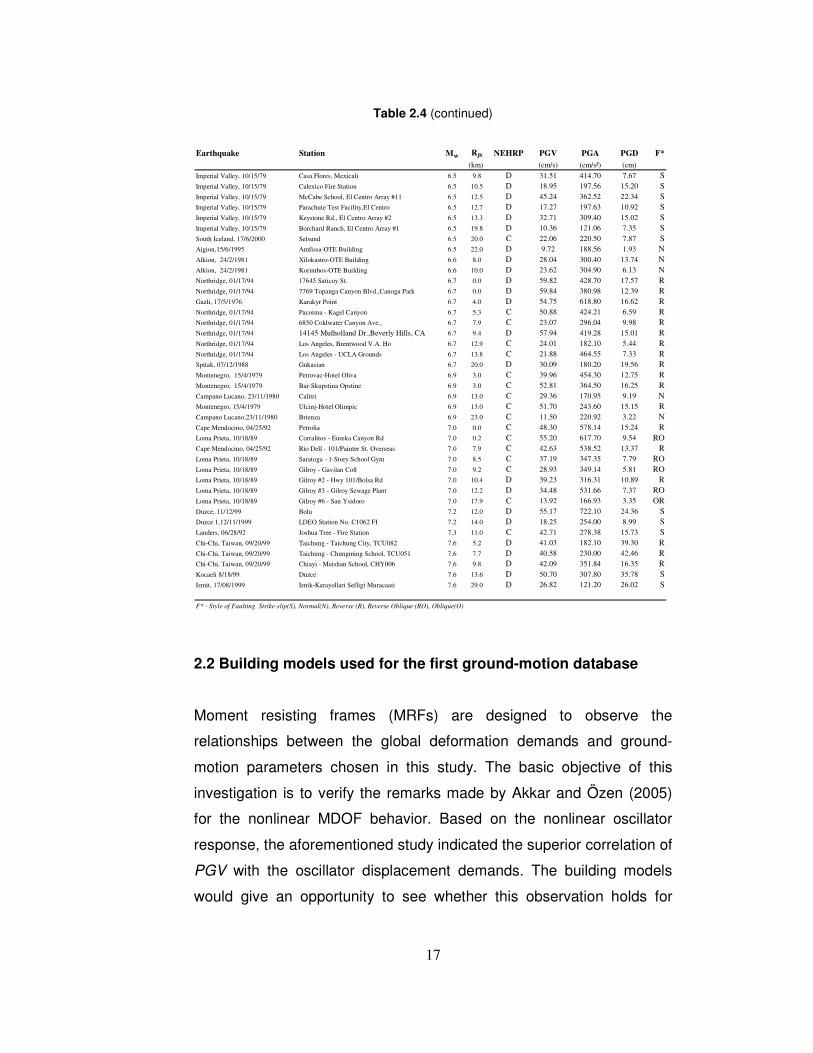
17
Table 2.4 (continued)
Earthquake Station Mw Rjb NEHRP PGV PGA PGD F*
(km) (cm/s) (cm/s²) (cm)
Imperial Valley, 10/15/79 Casa Flores, Mexicali 6.5 9.8 D 31.51 414.70 7.67 S
Imperial Valley, 10/15/79 Calexico Fire Station 6.5 10.5 D 18.95 197.56 15.20 S
Imperial Valley, 10/15/79 McCabe School, El Centro Array #11 6.5 12.5 D 45.24 362.52 22.34 S
Imperial Valley, 10/15/79 Parachute Test Facility,El Centro 6.5 12.7 D 17.27 197.63 10.92 S
Imperial Valley, 10/15/79 Keystone Rd., El Centro Array #2 6.5 13.3 D 32.71 309.40 15.02 S
Imperial Valley, 10/15/79 Borchard Ranch, El Centro Array #1 6.5 19.8 D 10.36 121.06 7.35 S
South Iceland, 17/6/2000 Selsund 6.5 20.0 C 22.06 220.50 7.87 S
Aigion,15/6/1995 Amfissa-OTE Building 6.5 22.0 D 9.72 188.56 1.93 N
Alkion, 24/2/1981 Xilokastro-OTE Building 6.6 8.0 D 28.04 300.40 13.74 N
Alkion, 24/2/1981 Korinthos-OTE Building 6.6 10.0 D 23.62 304.90 6.13 N
Northridge, 01/17/94 17645 Saticoy St. 6.7 0.0 D 59.82 428.70 17.57 R
Northridge, 01/17/94 7769 Topanga Canyon Blvd.,Canoga Park 6.7 0.0 D 59.84 380.98 12.39 R
Gazli, 17/5/1976 Karakyr Point 6.7 4.0 D 54.75 618.80 16.62 R
Northridge, 01/17/94 Pacoima - Kagel Canyon 6.7 5.3 C 50.88 424.21 6.59 R
Northridge, 01/17/94 6850 Coldwater Canyon Ave., 6.7 7.9 C 23.07 296.04 9.98 R
Northridge, 01/17/94 14145 Mulholland Dr.,Beverly Hills, CA 6.7 9.4 D 57.94 419.28 15.01 R
Northridge, 01/17/94 Los Angeles, Brentwood V.A. Ho 6.7 12.9 C 24.01 182.10 5.44 R
Northridge, 01/17/94 Los Angeles - UCLA Grounds 6.7 13.8 C 21.88 464.55 7.33 R
Spitak, 07/12/1988 Gukasian 6.7 20.0 D 30.09 180.20 19.56 R
Montenegro, 15/4/1979 Petrovac-Hotel Oliva 6.9 3.0 C 39.96 454.30 12.75 R
Montenegro, 15/4/1979 Bar-Skupstina Opstine 6.9 3.0 C 52.81 364.50 16.25 R
Campano Lucano, 23/11/1980 Calitri 6.9 13.0 C 29.36 170.95 9.19 N
Montenegro, 15/4/1979 Ulcinj-Hotel Olimpic 6.9 13.0 C 51.70 243.60 15.15 R
Campano Lucano,23/11/1980 Brienza 6.9 23.0 C 11.50 220.92 3.22 N
Cape Mendocino, 04/25/92 Petrolia 7.0 0.0 C 48.30 578.14 15.24 R
Loma Prieta, 10/18/89 Corralitos - Eureka Canyon Rd 7.0 0.2 C 55.20 617.70 9.54 RO
Cape Mendocino, 04/25/92 Rio Dell - 101/Painter St. Overseas 7.0 7.9 C 42.63 538.52 13.37 R
Loma Prieta, 10/18/89 Saratoga - 1-Story School Gym 7.0 8.5 C 37.19 347.35 7.79 RO
Loma Prieta, 10/18/89 Gilroy - Gavilan Coll 7.0 9.2 C 28.93 349.14 5.81 RO
Loma Prieta, 10/18/89 Gilroy #2 - Hwy 101/Bolsa Rd 7.0 10.4 D 39.23 316.31 10.89 R
Loma Prieta, 10/18/89 Gilroy #3 - Gilroy Sewage Plant 7.0 12.2 D 34.48 531.66 7.37 RO
Loma Prieta, 10/18/89 Gilroy #6 - San Ysidoro 7.0 17.9 C 13.92 166.93 3.35 OR
Duzce, 11/12/99 Bolu 7.2 12.0 D 55.17 722.10 24.36 S
Duzce 1,12/11/1999 LDEO Station No. C1062 FI 7.2 14.0 D 18.25 254.00 8.99 S
Landers, 06/28/92 Joshua Tree - Fire Station 7.3 11.0 C 42.71 278.38 15.73 S
Chi-Chi, Taiwan, 09/20/99 Taichung - Taichung City, TCU082 7.6 5.2 D 41.03 182.10 39.30 R
Chi-Chi, Taiwan, 09/20/99 Taichung - Chungming School, TCU051 7.6 7.7 D 40.58 230.00 42.46 R
Chi-Chi, Taiwan, 09/20/99 Chiayi - Meishan School, CHY006 7.6 9.8 D 42.09 351.84 16.35 R
Kocaeli 8/18/99 Duzce 7.6 13.6 D 50.70 307.80 35.78 S
Izmit, 17/08/1999 Iznik-Karayollari Sefligi Muracaati 7.6 29.0 D 26.82 121.20 26.02 S
F* - Style of Faulting Strike-slip(S), Normal(N), Reverse (R), Reverse Oblique (RO), Oblique(O)
2.2 Building models used for the first ground-motion database
Moment resisting frames (MRFs) are designed to observe the
relationships between the global deformation demands and ground-
motion parameters chosen in this study. The basic objective of this
investigation is to verify the remarks made by Akkar and Özen (2005)
for the nonlinear MDOF behavior. Based on the nonlinear oscillator
response, the aforementioned study indicated the superior correlation of
PGV with the oscillator displacement demands. The building models
would give an opportunity to see whether this observation holds for

18
model systems. The frame models are designed for the median design
spectra of the 3 bins that are assembled according to different PGV
ranges as described in Section 2.1. The median spectrum of each bin
assembled from the first ground-motion database as well as the
corresponding design spectra are presented in Figure 2.3. The smooth
design spectrum for each bin is obtained by following the procedure in
the FEMA 356 document. Five groups of reinforced concrete MRFs are
designed by making use of the three smoothed design spectra
described above. Each group contains 3, 5, 7 and 9 story regular
frames in compliance with the Turkish standards for Design and
Construction of RC structures, TS500 (TSE, 2000) and Turkish Seismic
Code (Bayındırlık ve İskan Bakanlığı, 1998).
0
0.2
0.4
0.6
0.8
1
1.2
0 1 2 3 4
T (s)
Sa
(g)
Bin 1 Acc.Resp.S.Bin 2 Acc.Resp.S.Bin 3 Acc.Resp.S.Bin 1 Design SpectrumBin 2 Design SpectrumBin 3 Design Spectrum
Figure 2.3 Median response and smoothed design spectra of the ground-motions assembled from the first ground-motion dataset. The abbreviations Sxs, Sx1 and Ts are the parameters used in the FEMA 356 document (ASCE, 2000) for the smoothed design spectrum.( Sxs and Sx1 represents the pseudo spectral acceleration at short and long periods,respectively. The variable Ts is the corner period that separates constant acceleration plateau from the descending branch)
Bin 1 Bin 2 Bin 3 Sxs = 0.36 Sxs = 0.81 Sxs = 0.9 Sx1 = 0.11 Sx1 = 0.27 Sx1 = 0.51 Ts = 0.30 Ts = 0.34 Ts = 0.52
PS
A (
g)

19
In all models, the story height and bay width are 3m and 5 m,
respectively. The compressive strength of concrete is 20MPa and the
yield strength of steel bars is 420 MPa. Rigid diaphragm assumption
was made and floor masses were lumped at the beam-column joints at
each story level. The Design Loads for Buildings, TS498 (TSE,
ACI1997) was used in the calculation of gravity loads (dead and live
loads). Design loads were calculated by using the provisions of the
aforementioned codes and the designed spectra presented in Figure
2.3. The dimensions of structural members are calculated by the
constraints imposed by the design spectrum and the design loads. The
column and beam dimensions were reduced with increasing height in
order to reflect the common design and construction practice. For 3
story models the column and beam dimensions remain constant
throughout the building height. In the case of 5 story models, the
column dimensions reduce after the 4th story and the beam dimensions
are kept constant. For 7 story models, both beam and column cross
sections reduce simultaneously at the 4th and 6th stories. The beam and
column dimensions are reduced at the 4th and 7th story levels for 9 story
models. The reduction in structural member dimensions is in
accordance with the Turkish seismic design code (TEC, 1998). The
reinforcement detailing of the frames are determined by using the
commercial software program SAP 2000 v.8.2.3 (CSI, 2000) and
therefore conformed to the provisions of ACI-318 (AC:I, 1999). A list
presenting the main properties of the analytical models is provided in
Table 2.5.
The model abbreviations in Table 2.5 describe the specific design
spectrum used in design of the buildings. For instance, e2 refers to the
design spectrum obtained from the second bin of the first ground-
motion database. The suit of building models e1' and e2' are obtained
by redesigning the corresponding e1 and e2 models for the design

20
spectrum of the third ground-motion bin. During the design of e1' and
e2', the geometric properties of e1 and e2 models were used whereas
the reinforcement detailing was modified according to the design
spectrum of the third ground-motion bin. This table contains the
sections, beam and column dimensions of each model as well as the
first mode periods and the post-yield stiffness ratios obtained from the
idealized pushover curves. Details of the frame models are provided in
Appendix A. Figure 2.4 shows a typical sketch of one of the 9 story
building models.
Table 2.5 Different properties of models
# of story Model T1 α Section Story h (cm) b (cm) # of story Model T1 α Section Story h (cm) b (cm)
e1 0.8203 0.0556 BEAM3 1-2-3 45.0 25.0 e3 COL1 1-2-3 50.0 50.0
COL3 1-2-3 30.0 30.0 COL2 4-5 45.0 45.0
e2 0.8156 0.0337 BEAM3 1-2-3 45.0 30.0 COL3 6-7 40.0 40.0
COL3 1-2-3 35.0 35.0 e1' 1.1400 0.0416 BEAM1 1-2-3 50.0 30.0
3 e3 0.8052 0.0274 BEAM3 1-2-3 50.0 30.0 BEAM2 4-5 50.0 30.0
COL3 1-2-3 45.0 45.0 BEAM3 6-7 45.0 30.0
e1' 0.6740 0.0598 BEAM3 1-2-3 45.0 25.0 7 COL1 1-2-3 40.0 40.0
COL3 1-2-3 30.0 30.0 COL2 4-5 35.0 35.0e2' 0.5667 0.0382 BEAM3 1-2-3 45.0 30.0 COL3 6-7 30.0 30.0
COL3 1-2-3 35.0 35.0 e2' 0.9513 0.0424 BEAM1 1-2-3 55.0 30.0
e1 1.0427 0.0558 BEAM2 1-2-3 45.0 25.0 BEAM2 4-5 50.0 30.0
BEAM3 4-5 45.0 25.0 BEAM3 6-7 50.0 30.0
COL2 1-2-3 35.0 35.0 COL1 1-2-3 45.0 45.0COL3 4-5 30.0 30.0 COL2 4-5 40.0 40.0
e2 0.7867 0.0394 BEAM2 1-2-3 50.0 30.0 COL3 6-7 35.0 35.0
BEAM3 4-5 50.0 30.0 e1 1.2964 0.0589 BEAM1 1-2-3 55.0 30.0
COL2 1-2-3 40.0 40.0 BEAM2 4-5-6 50.0 30.0
COL3 4-5 35.0 35.0 BEAM3 7-8-9 45.0 30.0
e3 0.6985 0.0274 BEAM2 1-2-3 50.0 30.0 COL1 1-2-3 45.0 45.0
5 BEAM3 4-5 50.0 30.0 COL2 4-5-6 40.0 40.0
COL2 1-2-3 45.0 45.0 COL3 7-8-9 35.0 35.0
COL3 4-5 40.0 40.0 e2 1.1213 0.0581 BEAM1 1-2-3 55.0 30.0
e1' 1.0163 0.0425 BEAM2 1-2-3 45.0 25.0 BEAM2 4-5-6 55.0 30.0
BEAM3 4-5 45.0 25.0 BEAM3 7-8-9 50.0 30.0
COL2 1-2-3 35.0 35.0 COL1 1-2-3 50.0 50.0
COL3 4-5 30.0 30.0 COL2 4-5-6 45.0 45.0
e2' 0.7788 0.0343 BEAM2 1-2-3 50.0 30.0 COL3 7-8-9 40.0 40.0
BEAM3 4-5 50.0 30.0 e3 0.9895 0.0373 BEAM1 1-2-3 60.0 30.0
COL2 1-2-3 40.0 40.0 9 BEAM2 4-5-6 55.0 30.0
COL3 4-5 35.0 35.0 BEAM3 7-8-9 50.0 30.0
e1 1.1516 0.0978 BEAM1 1-2-3 50.0 30.0 COL1 1-2-3 55.0 55.0
BEAM2 4-5 50.0 30.0 COL2 4-5-6 50.0 50.0
BEAM3 6-7 45.0 30.0 COL3 7-8-9 45.0 45.0
COL1 1-2-3 40.0 40.0 e1' 1.2827 0.0530 BEAM1 1-2-3 55.0 30.0
COL2 4-5 35.0 35.0 BEAM2 4-5-6 50.0 30.0
COL3 6-7 30.0 30.0 BEAM3 7-8-9 45.0 30.0
e2 0.9575 0.0531 BEAM1 1-2-3 55.0 30.0 COL1 1-2-3 45.0 45.0
7 BEAM2 4-5 50.0 30.0 COL2 4-5-6 40.0 40.0
BEAM3 6-7 50.0 30.0 COL3 7-8-9 35.0 35.0
COL1 1-2-3 45.0 45.0 e2' 1.1130 0.0435 BEAM1 1-2-3 55.0 30.0
COL2 4-5 40.0 40.0 BEAM2 4-5-6 55.0 30.0
COL3 6-7 35.0 35.0 BEAM3 7-8-9 50.0 30.0
e3 0.8715 0.0342 BEAM1 1-2-3 55.0 30.0 COL1 1-2-3 50.0 50.0
BEAM2 4-5 50.0 30.0 COL2 4-5-6 45.0 45.0
BEAM3 6-7 50.0 30.0 COL3 7-8-9 40.0 40.0

21
Figure 2.4 Typical sketch of 9 story analytical model. Note that column dimensions are reduced at the 4th and 7th story levels. The beam dimensions are also reduced at the same story levels
2.3 Nonlinear Response History Analyses of Frame Models Using
First Ground-Motion Dataset
As indicated in the previous section the relationship between some well
known ground-motion intensity measures and global deformation
demands of MDOF systems are investigated via nonlinear response
history analyses. The records in the first ground-motion database and
frames are used to achieve this objective. The details of the ground-
motions and building models are described in the previous section.
IDARC 2D (Valles et al, 1996) analysis program is used for running the
nonlinear response history analysis. The damage analysis model of
Modified Park-Ang-Wen is utilized by the program on single element
22
level and global structure level for the determination of inelastic
response. The program calculates the behavior of macro models in the
inelastic range by the distributed flexibility models that are suitable for
RC concrete elements and includes new hysteretic models upon which
the validation tests were conducted. The assumption of floor
diaphragms behaving as rigid horizontal links reduces the total
computational effort. For more information about the program IDARC-
2D capabilities and assumptions, the reader may refer to the technical
report NCEER-96-0010 (Valles et al., 1996).
Table 2.6 briefs the response history analysis conducted in this study.
The relationships between the global deformation demands (MRDR and
MIDR) and the ground-motion intensity measures (PGA, PGV and
PSa(T1)) are evaluated for 3 levels of nonlinear structural behavior: non-
degrading, stiffness degrading and stiffness and strength degrading.
Number of failures that occurred due to numerical stabilities in the
solution algorithm or structural collapses within each level of nonlinear
behavior and each model are also listed in the table. The built in tri-
linear hysteretic model of IDARC is modified to simulate these nonlinear
hysteretic behavior. The control parameters provided by IDARC-2D was
used for this purpose. Table 2.7 lists the control parameters used for
simulating various stiffness and strength degradation levels. The
designated values of stiffness degradation (α), ductility and energy
based strength degradation parameters (β1 and β2) as well as the slip
control parameter (γ) are suggested by the IDARC manual that are
verified by the test results of various structural members. As can be
depicted from these tabulated values the strength degradation is
governed by the energy dissipated during the cyclic excursions whereas
the role of slip in the reinforcing bars is disregarded in the cyclic
strength degradation of structural members.

2
3
Model GM Structural Failure Model GM Structural Failure Model GM Structural Failure Model GM Structural FailureUsed behavior in R.H.A. Used behavior in R.H.A. Used behavior in R.H.A. Used behavior in R.H.A.
e1 Bin 1 ND 0 / 20 e1 Bin 1 ND 0 / 20 e1 Bin 1 ND 0 / 20 e1 Bin 1 ND 0 / 20SD 0 / 20 SD 0 / 20 SD 0 / 20 SD 0 / 20
SSD 2 / 20 SSD 0 / 20 SSD 0 / 20 SSD 1 / 20e2 Bin 2 ND 0 / 20 e2 Bin 2 ND 0 / 20 e2 Bin 2 ND 0 / 20 e2 Bin 2 ND 0 / 20
SD 3 / 20 SD 4 / 20 SD 2 / 20 SD 0 / 20SSD 5 / 20 SSD 3 / 20 SSD 6 / 20 SSD 7 / 20
e3 Bin 1 ND 0 / 20 e3 Bin 1 ND 0 / 20 e3 Bin 1 ND 0 / 20 e3 Bin 1 ND 0 / 20SD 0 / 20 SD 0 / 20 SD 0 / 20 SD 0 / 20
SSD 0 / 20 SSD 0 / 20 SSD 0 / 20 SSD 0 / 20Bin 2 ND 0 / 20 Bin 2 ND 0 / 20 Bin 2 ND 0 / 20 Bin 2 ND 0 / 20
SD 1 / 20 SD 2 / 20 SD 1 / 20 SD 1 / 20SSD 2 / 20 SSD 1 / 20 SSD 5 / 20 SSD 7 / 20
Bin 3 ND 0 / 20 Bin 3 ND 0 / 20 Bin 3 ND 0 / 20 Bin 3 ND 0 / 20SD 3 / 20 SD 8 / 20 SD 5 / 20 SD 3 / 20
SSD 10 / 20 SSD 11 / 20 SSD 11 / 20 SSD 12 / 20e1' Bin 1 ND 0 / 20 e1' Bin 1 ND 0 / 20 e1' Bin 1 ND 0 / 20 e1' Bin 1 ND 0 / 20
SD 0 / 20 SD 0 / 20 SD 0 / 20 SD 0 / 20SSD 0 / 20 SSD 0 / 20 SSD 0 / 20 SSD 0 / 20
e2' Bin 2 ND 1 / 20 e2' Bin 2 ND 0 / 20 e2' Bin 2 ND 0 / 20 e2' Bin 2 ND 0 / 20SD 0 / 20 SD 1 / 20 SD 2 / 20 SD 0 / 20
SSD 5 / 20 SSD 7 / 20 SSD 4 / 20 SSD 7 / 20
Abbreviations : ND - Nondegrading, SD - Stiffness degrading, SSD - Stiffness and strength degrading, GM - Ground motions
R.H.A - Response history analysis
3 STORY 5 STORY 7 STORY 9 STORY
Table 2.6 Response history analysis conducted in the study

24
Table 2.7 Hysteretic model parameters used in the analysis
Hysteretic Model Non degrading Stiffness Degrading Stiffness and StrengthParameter (ND) (SD) Degrading (SSD)
α 200 4 4β1 0.01 0.01 0.6β2 0.01 0.01 0.01γ 1 1 1
Pushover curves obtained from the inverse triangular lateral loading
and their bilinear idealizations in compliance with the methodology
presented in ATC 40 document (ATC, 1996) are presented for each
model in Appendix B (Figures B1-B15). The pushover curve of each
model is displayed both in terms of base shear coefficient (η) vs. roof
displacement (∆roof) and acceleration vs displacement response
spectrum (ADRS) formats. The expressions used for the ADRS format
are also presented in ATC-40 (ATC, 1996). The maximum observed
base shear and roof displacement pairs are compiled from response
analysis are also superimposed on these plots to investigate whether
the model buildings are mostly deformed under the first mode dominant
structural behavior. Note that the response history analysis results that
are superimposed in the global capacity curves (pushover curves)
suggest that the building models are generally subjected to moderate to
large lateral deformation demands except for the e1’ building models.
The deformation demands computed from the response history analysis
of e1’ model buildings are mostly within the elastic limits (Figures B.4,
B.9 and B.14). This is quite expected because e1’ model buildings are
subjected to the records that contain the lowest PGVs (i.e. they mirror
relatively the lowest hazard level). Contradictory to the e1, they are
designed for the design spectrum that relatively represents the highest
hazard level (i.e. for the ground motion bin with the highest PGV values.
Although the existence of some significant differences between the
pushover curves and maximum absolute η-∆roof pairs obtained from

25
response history analysis, the buildings seem to predominantly under
the fundamental mode. The reason behind the conclusion is that for
most cases as displayed in Appendix B, the maximum absolute η-∆roof
scatter points follow the pushover curve patterns closely that are
computed from the inverse triangular loading pretending to mimic
fundamental mode global capacity. Thus, the succeeding discussion for
the relationships between the chosen ground-motion intensity
parameters and global deformation demands are confined to the
building behavior deforming primarily under first mode response.
It should be noted that the influence of p-delta effect is not considered
in the nonlinear response history analyses since a series of pushover
analyses with different hysteretic behaviors resulted in a very similar
global response curves with and without p-delta effects. This
observation may also suggest that the IDARC-2D does not incorporate
p-delta effects in the nonlinear structural response although the
software seems to provide an option for the consideration of second
order effects in nonlinear structural response.
The variation of three ground-motion intensity parameters (PGA, PGV
and PSa(T1) ) with global deformation demands (MIDR and MRDR) is
presented in Figures 2.5 - 2.10 for frame type building behavior having
fundamental periods between 0.60<T1<1.3 s. The scatter diagrams in
Figure 2.5 and 2.6 display the performance of chosen ground-motion
intensity parameters for non-degrading building behavior as a function
of MRDR and MIDR, respectively. Figures 2.7 to 2.8 and 2.9 to 2.10
present similar comparisons for stiffness degrading and stiffness and
strength degrading structural behavior, respectively. Each scatter
diagram contains the nonlinear response history results of five different
models (e1, e2, e3, e1’ and e2’) between the chosen IM’s and demand
parameters for frame buildings subjected to records associated with
low-to-high amplitude peak motions and spectral quantities of their

26
fundamental periods. Note that the scatter plots do not present the
nonlinear response history results when the model buildings showed
collapse behavior or when IDARC-2D experienced numerical problems
during the analysis stage. In each figure, the panels in the 1st, 2nd, 3rd
and 4th rows display the scatter plots for 3, 5, 7 and 9 story models,
respectively. Similarly, the three columns from left to right display the
relationship between the chosen demand parameters with PGA, PGV
and PSa(T1), respectively. In general, the increase in intensity measures
results in an increase in demand parameters. However the scatter (or
dispersion) in the increasing trends is significant for some cases.
Therefore, an unbiased statistical index is required to measure the
correlation between the chosen IMs and the demand parameters. This
is discussed in the next paragraph.
Spearman’s non-parametric coefficient (ρ) is used to assess the
correlation between the intensity measures and demand parameters
(Equation 2.1). This correlation index does not assume a linear
relationship between the variables. It also does not require any
assumption about he frequency distribution of the variables (Press et al,
1989). These features make Spearman’s coefficient more versatile then
the conventional correlation coefficient parameter since the latter is only
valid for normally distributed variables. High ρ values suggest higher
correlation on the linearity between the variables under investigation.
The Spearman’s non-parametric coefficients are displayed on each
panel in Figures 2.5 to 2.10.
)1(
61
2
2
−−=∑nn
d iρ (2.1)
di : the difference between each rank of corresponding values of x and y
n : number of pairs of values

27
1 10 100
1 10 100 0.01 0.1 10.01
0.1
1
0.01 0.1 10.01
0.1
1
1 10 100 0.01 0.1 10.01
0.1
1
PGV (cm/s)
1 10 100
PSa(T1) (g)
0.01 0.1 10.01
0.1
1
100 1000
MR
DR
(%
)
0.01
0.1
1
100 1000
MR
DR
(%
)
0.01
0.1
1
100 1000
MR
DR
(%
)
0.01
0.1
1
PGA (cm/s2)
100 1000
MR
DR
(%
)
0.01
0.1
1
Figure 2.5 Variation of MRDR with PGA, PGV and PSa(T1) for nondegrading building models
ρ=0.571 ρ=0.601 ρ=0.534
ρ=0.597 ρ=0.656 ρ=0.610
ρ=0.492 ρ=0.586 ρ=0.475
ρ=0.620 ρ=0.738 ρ=0.597
3 st.
T1=0.41-0.73
5 st.
T1=0.70-1.04
7 st.
T1=0.87-1.15
9 st.
T1=0.99-1.30

28
1 10 100 0.01 0.1 10.01
0.1
1
1 10 100 0.01 0.1 10.01
0.1
1
1 10 100 0.01 0.1 10.01
0.1
1
PGV (cm/s)
1 10 100 0.01 0.1 10.01
0.1
1
100 1000
MID
R (
%)
0.01
0.1
1
100 1000
MID
R (
%)
0.01
0.1
1
100 1000
MID
R (
%)
0.01
0.1
1
PGA (cm/s2)
100 1000
MID
R (
%)
0.01
0.1
1
PSa(T1) (g)
Figure 2.6 Variation of MIDR with PGA, PGV and PSa(T1) for Nondegrading building models
ρ=0.568 ρ=0.600 ρ=0.529 3 st.
T1=0.41-0.73
ρ=0.615 ρ=0.687 ρ=0.620 5 st.
T1=0.70-1.04
ρ=0.578 ρ=0.683 ρ=0.545 7 st.
T1=0.87-1.15
ρ=0.605 ρ=0.709 ρ=0.565 9 st.
T1=0.99-1.30

29
1 10 100100 1000
MR
DR
(%
)
0.01
0.1
1
0.01 0.1 10.01
0.1
1
100 1000
MR
DR
(%
)
0.01
0.1
1
1 10 100 0.01 0.1 10.01
0.1
1
100 1000
MR
DR
(%
)
0.01
0.1
1
PGV (cm/s)
1 10 100 0.01 0.1 10.01
0.1
1
PGA (cm/s2)
100 1000
MR
DR
(%
)
0.01
0.1
1
0.01 0.1 10.01
0.1
1
1 10 100
PSa(T1) (g)
Figure 2.7 Variation of MRDR with PGA, PGV and PSa(T1) in Stiffness degrading building models
ρ=0.623 ρ=0.605 ρ=0.566
ρ=0.503 ρ=0.597 ρ=0.561
ρ=0.508 ρ=0.576 ρ=0.510
ρ=0.638 ρ=0.759 ρ=0.633

30
1 10 100100 1000
MID
R (
%)
0.01
0.1
1
10
0.01 0.1 10.01
0.1
1
10
1 10 100100 1000
MID
R (
%)
0.01
0.1
1
10
0.01 0.1 10.01
0.1
1
10
100 1000
MID
R (
%)
0.01
0.1
1
10
PSa (T1) (g)
0.01 0.1 10.01
0.1
1
10
PGA (cm/s2)
10 100 1000
MID
R (
%)
0.01
0.1
1
10
0.01 0.1 10.01
0.1
1
10
PGV (cm/s)
1 10 100
1 10 100
Figure 2.8 Variation of MIDR with PGA, PGV and PSa(T1) for Stiffness degrading building models
ρ=0.564 ρ=0.604 ρ=0.559
ρ=0.577 ρ=0.626 ρ=0.555
ρ=0.605 ρ=0.698 ρ=0.605
ρ=0.613 ρ=0.735 ρ=0.614

31
1 10 100 0.01 0.1 10.01
0.1
1
1 10 100 0.01 0.1 10.01
0.1
1
1 10 100 0.01 0.1 10.01
0.1
1
PGV (cm/s)
1 10 100 0.01 0.1 10.01
0.1
1
100 1000
MR
DR
(%
)
0.01
0.1
1
100 1000
MR
DR
(%
)
0.01
0.1
1
100 1000
MR
DR
(%
)
0.01
0.1
1
PGA (cm/s2)
100 1000
MR
DR
(%
)
0.01
0.1
1
PSa(T1) (g)
Figure 2.9 Variation of MRDR with PGA, PGV and PSa(T1) for Stiffness and strength degrading building models
ρ=0.612 ρ=0.565 ρ=0.533
ρ=0.559 ρ=0.654 ρ=0.570
ρ=0.516 ρ=0.584 ρ=0.515
ρ=0.669 ρ=0.702 ρ=0.613

32
1 10 100 0.01 0.1 10.01
0.1
1
1 10 100 0.01 0.1 10.01
0.1
1
1 10 100 0.01 0.1 10.01
0.1
1
PGV (cm/s)
1 10 100 0.01 0.1 10.01
0.1
1
100 1000
MID
R (
%)
0.01
0.1
1
100 1000
MID
R (
%)
0.01
0.1
1
100 1000
MID
R (
%)
0.01
0.1
1
PGA (cm/s2)
100 1000
MID
R (
%)
0.01
0.1
1
PSa(T1) (g)
Figure 2.10 Variation of MIDR with PGA, PGV and PSa(T1) for Stiffness and strength degrading building models
ρ=0.612 ρ=0.559 ρ=0.525
ρ=0.566 ρ=0.644 ρ=0.561
ρ=0.594 ρ=0.651 ρ=0.579
ρ=0.656 ρ=0.683 ρ=0.577

33
Table 2.8 and Figure 2.11 also display the computed ρ values to
summarize the relationship between the chosen IMs and demand
parameters in terms of this statistical index.
Table 2.8 Spearman’s coefficient values (ρ) between intensity measures and global demand parameters under three different structural behavior
Structural IntensityBehavior Measure 3 story 5 story 7 story 9 story 3 story 5 story 7 story 9 story
PGA 0.571 0.597 0.492 0.620 0.568 0.615 0.578 0.605ND PGV 0.601 0.656 0.586 0.738 0.600 0.687 0.683 0.709
PSA 0.534 0.610 0.475 0.597 0.529 0.620 0.545 0.565PGA 0.623 0.503 0.508 0.638 0.564 0.577 0.605 0.613
SD PGV 0.605 0.597 0.576 0.759 0.604 0.626 0.698 0.735PSA 0.566 0.561 0.510 0.633 0.559 0.555 0.605 0.614PGA 0.612 0.559 0.516 0.669 0.612 0.566 0.594 0.656
SSD PGV 0.565 0.654 0.584 0.702 0.559 0.644 0.651 0.683PSA 0.533 0.570 0.515 0.613 0.525 0.561 0.579 0.577
MRDR MIDR
MRDR- Non degrading
PGV
ρ
0.45
0.50
0.55
0.60
0.65
0.70
0.75
0.80
PSAPGA
MRDR Stiffness degrading
PGV PSAPGA
MRDR Stf. and strength degrading
PGV
0.45
0.50
0.55
0.60
0.65
0.70
0.75
0.80
PSAPGA
3 story 5 story 7 story 9 story
MIDR- Non degrading
PGV
ρ
0.45
0.50
0.55
0.60
0.65
0.70
0.75
0.80
PSAPGA
MIDR Stiffness degrading
PGV PSAPGA
MIDR Stf. and strength degrading
PGV
0.45
0.50
0.55
0.60
0.65
0.70
0.75
0.80
PSAPGA
3 story 5 story 7 story 9 story
Figure 2.11 Comparison of the Spearman’ s correlation coefficient values of ground motion intensity measures with global demand measures

34
The observations drawn from these figures and Table 2.8 are written
below:
1. Regardless of the hysteretic behavior ρ values for PGV vs.
MRDR and PGV vs. MIDR tend to increase with increasing story
number.
2. When ρ values computed for all three ground-motion intensity
measures are considered, those associated with PGV are larger
than those computed for PGA and PSa(T1).
3. When PGA vs. MRDR and PGA vs. MIDR relationships are of
concern, there is no clear relationship between the associated ρ
values and the story number.
4. There seems to be a consistent trend between ρ and story
number when PSa(T1) vs. MRDR and PSa(T1) vs. MIDR
relationships are evaluated. However, the associated ρ values
generally attain smaller values with respect to those computed
for PGV and PGA. For this particular IM, the consistent increase
in ρ with the increasing story number may advocate that the
building models predominantly behave under the fundamental
mode influence. This is because many researchers (e.g. Curballa
et al, 2002) stated that PSa(T1) is not a good indicator of damage
for studies that are dominated by higher mode effects.
The general tendency of increase in the correlation values of PGA and
MRDR is distinguishable with the increasing story numbers except for 5
story model. Similar observation is valid for PGA and MIDR relation.
However, the relation of PGV with MRDR reveals a clear decrease in
stiffness degrading case for 5 and 7 story models when the different

35
degrading situations are considered whereas higher values are seen for
3 and 9 stories. A different situation is noted for PGV-MIDR relation.
The value of 5 story is lower in stiffness degrading case, while those of
the other story models are higher than ρ values of other degradation
situations. The variation of PSa(T1) with MRDR and MIDR exhibits
similarities. For 3, 5 and 9 story models, ρ value increases in general
sense and highest correlation values among different structural
behaviors are observed in stiffness degrading case.
Note that some of the observations indicated above are open to further
discussion. In general, PGA is generally referred to as a poor indicator
of structural damage that is closely related to MRDR and MIDR.
However, the results presented in this study show that there seems to
be no appreciable differences between the performance of PGA and
PSa(T1) when establishing relationships with these IMs and the demand
parameters considered. Moreover, the analyses presented here
indicate that PGV is a better indicator of the deformation demand than
PGA and PSa(T1) that is also questioned by some recent studies (e.g.
Yılmaz, 2007; Riddell, 2007).
The conclusions made in this chapter are confined to the ground-motion
database used by Akkar and Özen (2005) and the building models
presented. These findings should be verified by other studies for
different ground-motion datasets and for different building models in
order to investigate the disagreements between this study and other
studies. Nevertheless, the good performance of PGV with respect to the
other two IMs studied in this chapter stimulated this study to propose
regression models for PGV to estimate inelastic oscillator displacement
demands. This is described in detail in the next chapter.

36
CHAPTER 3
ESTIMATION OF INELASTIC SPECTRAL DISPLACEMENTS AS A
FUNCTION OF PEAK GROUND VELOCITY
3.1 Introduction
The limited number of statistical results presented in Chapter 2
suggested that PGV can be considered as a candidate intensity
measure for bridging the gaps between earthquake hazard and
deformation demands on structural systems. This chapter presents a
simple predictive model that can be used in estimating peak oscillator
displacements as a function of PGV. The predictive model can be used
for estimating constant ductility (µ) and normalized lateral strength (R)
spectral displacements for a given initial oscillator periods. The constant
ductility and normalized lateral strength displacement spectra can be
used for design and seismic performance evaluation of structural
systems (FEMA-356, ATC-40, FEMA- 44, Fajfar, 2000). The
succeeding sections of this chapter first describe the regression model
and then present a simple case study to show its implementation.
3.2 Regression Analysis
The general mathematical model for estimating the peak nonlinear
oscillator displacement (Sd,ie) for a given µ or R value is given in Eq.
(3.1).
TPGVfSRied ⋅⋅= )(
,, θµ
(3.1)

37
The functional form f in Eq. (3.1) considers the influence of independent
ground-motion parameters (θ) such as magnitude, distance, site class
etc. for the estimation of Sd,ie. The regression analysis was conducted
on the dimensionless dependent variable Sd,ie/(PGV×T) because this
parameter resulted in a simpler predictive model as discussed in the
next paragraphs. The influence of independent ground-motion
parameters on the predicted parameter was investigated by studying
the behavior of Sd,e/(PGV×T) that is the elastic response version of the
predicted parameter. Some recent ground-motion prediction equations
(GMPEs) that estimate both PGV and Sd,e were used to achieve this
objective.
The main assumption in this sensitivity analysis is that the general
behavior of the predicted parameter will have a similar (but not the
same) pattern both in the linear and nonlinear oscillator response.
Figure 3.1 shows the comparative results from two recent GMPEs that
are derived by Akkar and Bommer (2007a, 2007b) and Boore and
Atkinson (2007). Functional forms and brief information about the
prediction equations are given in Appendix C. These GMPEs are
abbreviated as AB07 and BA07, respectively. The figures on the left
display the results computed from AB07 whereas the pertaining results
of BA07 are presented on the right hand side. The AB07 prediction
equations were derived from a recently compiled European ground-
motion database. The BA07 GMPE uses a worldwide ground-motion
dataset that is compiled for Next Generation Attenuation (NGA) project.
Both studies estimate the spectral and peak ground-motion quantities
with certain differences in their functional forms. For example BA07
considers the nonlinear soil effects as a function of Vs,30 whereas AB07
does not account for soil nonlinearity in the predictive model. The first
row in Figure 3.1 shows the influence of distance metric (Rjb) on
Sd,e/(PGV×T) for the magnitude range of interest in this study. The

38
figures on the left and right panels display 3 set of curves for oscillator
periods of T = 0.5, 1.0 and 2.0 s and each set compares 3 distinct Rjb
distances (i.e. Rjb = 10, 20 and 30 km) for a given oscillator period.
The discrete T and Rjb values presented fairly cover the period and
distance ranges in this study. All plots are produced for strike-slip
events. The comparative plots show that for short-period oscillator
response (T = 0.5 s) both GMPEs describe a slight departure for the Rjb
= 10 km curve with respect to the Rjb = 20 and 30 km curves in the
small magnitude range. As far as the long-period oscillator response (T
= 2.0 s) is concerned, the AB07 curves follow a trend similar to the one
described for T = 0.5 s whereas BA07 curves almost overlap each other
for all Rjb distances. The differences between the GMPEs for T = 2.0 s
may arise from their distinct magnitude scaling functional forms. The
GMPEs considered do not show a distance-wise sensitivity for T = 1.0
s. Although it is crude, these observations may lead to an assumption
that the discrepancies on Sd,e/(PGV×T) emerging from distance
variation are secondary when compared to the magnitude influence.
The second row in Figure 3.1 shows the significance of site class on
Sd,e/(PGV×T). NEHRP site classes C and D are considered in the
comparative plots as the ground-motion dataset consists of records
from these site categories.
Akkar and Bommer (2007a, 2007b) classified NEHRP C and D site
classes as stiff and soft soils, respectively. Boore and Atkinson (2007)
does not use a specific site classification since their predictive model
directly uses the Vs,30 values. For illustrative purposes Vs,30 = 450 m/s
and 270 m/s are used in BA07 to represent stiff and soft soil sites,
respectively. Each panel displays 3 sets of Sd,e/(PGV×T) vs. Rjb curves
computed for T = 0.5, 1.0 and 2.0 s. Each set corresponds to a
particular oscillator period and shows the variation in Sd,e/(PGV×T) for

39
stiff and soft sites, respectively. In order not to crowd the figures AB07
predictions were used for displaying the results for M = 7 whereas BA07
was used to illustrate the results from small magnitude events mimicked
by M = 5. Similar to the first row plots, the style-of-faulting is strike-slip
in these figures.
Akkar and Bommer (2007)
Magnitude (M)5 6 7
Sd,
e/(P
GV
xT)
0.05
0.060.070.080.09
0.2
0.3
0.4
0.1
T=0.5s, rjb=10kmT=0.5s, rjb=20kmT=0.5s, rjb=30kmT=1.0s, rjb=10kmT=1.0s, rjb=20kmT=1.0s, rjb=30kmT=2.0s, rjb=10kmT=2.0s, rjb=20kmT=2.0s, rjb=30km
Boore and Atkinson (2007)
Magnitude (M)5 6 7
0.05
0.060.070.080.09
0.2
0.3
0.4
0.1
T=0.5s, rjb=10kmT=0.5s, rjb=20kmT=0.5s, rjb=30kmT=1.0s, rjb=10kmT=1.0s, rjb=20kmT=1.0s, rjb=30kmT=2.0s, rjb=10kmT=2.0s, rjb=20kmT=2.0s, rjb=30km
T=0.5sT=0.5s
T=1.0s
T=1.0s
T=2.0s
T=2.0s
Stiff Site Vs,30 = 450 m/s
Distance, Rjb (km)
0 5 10 15 20 25 30
Sd,
e/(P
GV
xT)
0.00
0.05
0.10
0.15
0.20
0.25
0.30
Stiff, T = 0.5sSoft, T = 0.5sStiff, T = 1.0sSoft, T = 1.0sStiff, T = 2.0sSoft, T = 0.5s
Distance, Rjb (km)
0 5 10 15 20 25 300.00
0.05
0.10
0.15
0.20
0.25
0.30
Vs,30 = 450m/s, T = 0.5sVs,30 = 270m/s, T = 0.5sVs,30 = 450m/s, T = 1.0sVs,30 = 270m/s, T = 1.0sVs,30 = 450m/s, T = 2.0sVs,30 = 270m/s, T = 2.0s
M = 7 M = 5
Figure 3.1. Influence of certain ground-motion parameters on Sd,e/(PGV×T).
Although there is a departure in Sd,e/(PGV×T) between soft and stiff soil
sites for large magnitude and mid-period values (T = 1.0 s), the general
picture from these plots may also advocate that magnitude is a more
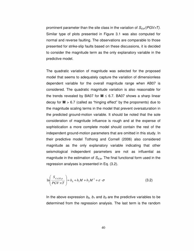
40
prominent parameter than the site class in the variation of Sd,e/(PGV×T).
Similar type of plots presented in Figure 3.1 was also computed for
normal and reverse faulting. The observations are comparable to those
presented for strike-slip faults based on these discussions, it is decided
to consider the magnitude term as the only explanatory variable in the
predictive model.
The quadratic variation of magnitude was selected for the proposed
model that seems to adequately capture the variation of dimensionless
dependent variable for the overall magnitude range when AB07 is
considered. The quadratic magnitude variation is also reasonable for
the trends revealed by BA07 for M ≤ 6.7. BA07 shows a sharp linear
decay for M > 6.7 (called as “hinging effect” by the proponents) due to
the magnitude scaling terms in the model that prevent oversaturation in
the predicted ground-motion variable. It should be noted that the sole
consideration of magnitude influence is rough and at the expense of
sophistication a more complete model should contain the rest of the
independent ground-motion parameters that are omitted in this study. In
their predictive model Tothong and Cornell (2006) also considered
magnitude as the only explanatory variable indicating that other
seismological independent parameters are not as influential as
magnitude in the estimation of Sd,ie. The final functional form used in the
regression analyses is presented in Eq. (3.2).
σεµ
⋅+++=
×2
210
,,ln MbMbb
TPGV
SRied
(3.2)
In the above expression b0, b1 and b2 are the predictive variables to be
determined from the regression analysis. The last term is the random

41
error term and it accounts for the variability in the dependent parameter
due to the unconsidered predictor parameters in the model.
This term corresponds to the difference between the estimated and
observed dependent variable that is called the residual in the regression
analysis. If the fitted model correctly accounts for the variation of the
observed data, the residual mean square is the unbiased estimator of
the variance (σ2) about the regression. However, if the model fails to
explain the variation of observed data, the residuals contain both
random and systematic errors due to model inadequacy resulting in
biased σ2 calculated from the residual mean square (Drapper and
Smith, 1981). The ε in Eq. (3.2) denotes the number of standard
deviations (σ) above or below the expected value of dependent
variable.
There are number of regression techniques to estimate the predictive
variables of a functional form. In this study the least squares regression
was used that would estimate the same predictive variables as of
maximum likelihood regression method given the random error terms
are normally distributed with zero mean and σ2 (Myers, 1986). This
condition is satisfied here as discussed in the succeeding paragraphs.
The regressions were done by period-by-period for 0.2s ≤ T ≤ 2.0s with
increments of 0.1 s. The inelastic oscillator displacements are estimated
at 8 distinct µ and R values (i.e. µ or R = 1.5, 2, 3, 4, 5, 6, 7 and 8) for
bilinear hysteretic model associated with 0% and 5% postyield stiffness
ratio (α). The initial damping was taken as 5% of critical in all nonlinear
oscillator responses. Tables 3.1-3.4 present four sets of regression
coefficients in terms of µ and R as well as for the α values stated
above.

42
Table 3.1 Regression coefficients for constant µ peak inelastic oscillator displacements when α = 0%
T (s) b0 b1 b2 σ b0 b1 b2 σ b0 b1 b2 σ b0 b1 b2 σ
0.2 -7.841 2.220 -0.204 0.451 -7.585 2.135 -0.195 0.431 -6.522 1.800 -0.166 0.368 -5.624 1.526 -0.142 0.358
0.3 -3.547 0.837 -0.085 0.371 -1.322 0.107 -0.025 0.361 -1.763 0.222 -0.029 0.330 -2.245 0.411 -0.045 0.315
0.4 -2.906 0.656 -0.069 0.368 -3.888 0.931 -0.087 0.330 -2.824 0.585 -0.057 0.297 -1.973 0.334 -0.037 0.279
0.5 -7.760 2.098 -0.172 0.327 -5.573 1.404 -0.117 0.300 -3.059 0.654 -0.060 0.306 -3.419 0.783 -0.070 0.292
0.6 -1.860 0.185 -0.018 0.348 -1.880 0.150 -0.012 0.318 -1.564 0.106 -0.011 0.311 -1.783 0.163 -0.013 0.298
0.7 -2.447 0.343 -0.028 0.342 -1.612 0.038 -0.001 0.331 -2.814 0.406 -0.028 0.353 -3.033 0.448 -0.027 0.334
0.8 -1.063 -0.121 0.010 0.343 -2.435 0.261 -0.016 0.323 -3.730 0.687 -0.049 0.337 -2.468 0.259 -0.013 0.343
0.9 -1.370 -0.113 0.016 0.351 -0.457 -0.397 0.037 0.337 -3.384 0.533 -0.035 0.337 -4.146 0.729 -0.046 0.345
1.0 -0.172 -0.490 0.045 0.340 1.668 -1.046 0.086 0.347 -3.184 0.376 -0.016 0.343 -6.418 1.362 -0.090 0.355
1.1 -0.979 -0.283 0.032 0.349 -3.590 0.509 -0.028 0.334 -7.184 1.588 -0.107 0.339 -9.271 2.241 -0.157 0.350
1.2 -3.702 0.482 -0.022 0.367 -7.283 1.619 -0.111 0.370 -10.673 2.656 -0.189 0.370 -10.053 2.443 -0.170 0.380
1.3 -5.969 1.190 -0.077 0.395 -6.517 1.358 -0.090 0.399 -9.690 2.333 -0.164 0.395 -8.921 2.052 -0.138 0.399
1.4 -6.199 1.195 -0.073 0.381 -6.225 1.222 -0.077 0.378 -9.002 2.052 -0.137 0.423 -8.391 1.891 -0.127 0.408
1.5 -4.936 0.712 -0.029 0.389 -5.305 0.847 -0.041 0.393 -10.073 2.352 -0.159 0.415 -7.012 1.360 -0.079 0.431
1.6 -6.997 1.356 -0.080 0.404 -7.248 1.391 -0.080 0.400 -7.326 1.425 -0.083 0.424 -5.470 0.843 -0.038 0.459
1.7 -7.233 1.414 -0.084 0.427 -7.325 1.445 -0.087 0.418 -7.608 1.558 -0.099 0.441 -5.228 0.749 -0.030 0.464
1.8 -8.038 1.653 -0.102 0.423 -6.752 1.248 -0.072 0.427 -6.545 1.184 -0.067 0.447 -4.348 0.408 0.001 0.466
1.9 -9.438 2.079 -0.135 0.437 -7.387 1.414 -0.082 0.446 -5.455 0.777 -0.031 0.451 -4.653 0.463 -0.001 0.476
2.0 -7.904 1.565 -0.093 0.444 -7.251 1.321 -0.072 0.470 -4.439 0.390 0.004 0.465 -4.183 0.324 0.008 0.489
T (s) b0 b1 b2 σ b0 b1 b2 σ b0 b1 b2 σ b0 b1 b2 σ
0.20 -5.564 1.520 -0.139 0.343 -5.276 1.446 -0.133 0.336 -5.069 1.387 -0.127 0.324 -4.757 1.297 -0.118 0.317
0.30 -2.306 0.453 -0.048 0.308 -2.120 0.415 -0.045 0.298 -2.323 0.491 -0.050 0.291 -3.808 0.942 -0.083 0.281
0.40 -1.845 0.280 -0.030 0.275 -1.397 0.146 -0.018 0.272 -0.691 -0.076 0.000 0.279 -0.813 -0.037 -0.002 0.282
0.50 -2.103 0.365 -0.036 0.290 -0.642 -0.106 0.003 0.294 -1.583 0.166 -0.016 0.304 -0.939 -0.036 0.001 0.317
0.60 -1.504 0.054 -0.002 0.314 -1.429 0.026 0.002 0.326 -2.930 0.485 -0.032 0.330 -3.377 0.636 -0.044 0.332
0.70 -2.082 0.156 -0.004 0.335 -2.117 0.160 -0.003 0.335 -2.006 0.108 0.003 0.332 -2.013 0.115 0.003 0.332
0.80 -1.693 -0.016 0.012 0.346 -3.299 0.508 -0.030 0.347 -4.618 0.913 -0.060 0.352 -4.754 0.955 -0.063 0.359
0.90 -4.724 0.926 -0.061 0.344 -6.363 1.418 -0.097 0.339 -8.393 2.023 -0.141 0.339 -9.169 2.251 -0.157 0.346
1.00 -7.568 1.719 -0.116 0.352 -9.540 2.317 -0.160 0.352 -9.462 2.273 -0.155 0.359 -10.330 2.541 -0.175 0.362
1.10 -10.401 2.552 -0.178 0.361 -11.002 2.730 -0.190 0.372 -10.290 2.497 -0.171 0.385 -9.687 2.301 -0.155 0.407
1.20 -10.235 2.466 -0.169 0.386 -9.871 2.321 -0.155 0.405 -8.620 1.912 -0.121 0.425 -8.046 1.734 -0.108 0.431
1.30 -7.793 1.660 -0.104 0.403 -8.139 1.745 -0.109 0.432 -7.299 1.476 -0.087 0.455 -6.607 1.256 -0.070 0.456
1.40 -7.282 1.473 -0.089 0.439 -6.111 1.081 -0.056 0.459 -5.730 0.946 -0.044 0.469 -5.305 0.796 -0.031 0.470
1.50 -4.805 0.638 -0.021 0.460 -5.097 0.735 -0.029 0.478 -4.757 0.610 -0.017 0.485 -4.236 0.428 -0.001 0.486
1.60 -4.245 0.454 -0.007 0.472 -3.788 0.291 0.008 0.475 -3.693 0.233 0.015 0.471 -3.444 0.140 0.023 0.456
1.70 -3.974 0.316 0.007 0.464 -3.443 0.126 0.024 0.463 -2.435 -0.195 0.050 0.446 -4.467 0.464 -0.004 0.452
1.80 -3.018 -0.028 0.037 0.468 -2.642 -0.145 0.046 0.459 -4.346 0.395 0.003 0.457 -4.032 0.299 0.011 0.462
1.90 -3.680 0.161 0.022 0.477 -3.114 0.006 0.033 0.473 -3.777 0.206 0.018 0.477 -2.932 -0.068 0.041 0.478
2.00 -3.232 0.012 0.034 0.491 -2.630 -0.177 0.049 0.485 -2.757 -0.143 0.047 0.489 -4.728 0.456 0.002 0.483
µ = 5.0 µ = 6.0 µ = 7.0 µ = 8.0
µ = 1.5 µ = 3 µ = 4µ = 2.0

43
Table 3.2. Regression coefficients for constant µ peak inelastic oscillator displacements when α = 5%
T (s) b0 b1 b2 σ b0 b1 b2 σ b0 b1 b2 σ b0 b1 b2 σ
0.2 -8.054 2.281 -0.209 0.448 -7.669 2.153 -0.197 0.427 -7.044 1.938 -0.176 0.361 -6.586 1.797 -0.162 0.342
0.3 -3.580 0.847 -0.086 0.372 -2.082 0.340 -0.044 0.358 -3.075 0.664 -0.068 0.317 -3.580 0.835 -0.080 0.297
0.4 -3.031 0.690 -0.071 0.367 -4.262 1.039 -0.096 0.320 -3.315 0.729 -0.069 0.296 -3.212 0.701 -0.066 0.273
0.5 -8.143 2.210 -0.180 0.328 -5.764 1.467 -0.123 0.301 -4.657 1.145 -0.099 0.290 -3.621 0.808 -0.071 0.262
0.6 -1.878 0.186 -0.018 0.345 -1.504 0.034 -0.004 0.311 -1.560 0.073 -0.008 0.294 -2.670 0.414 -0.033 0.281
0.7 -2.416 0.336 -0.028 0.338 -0.861 -0.192 0.016 0.317 -4.599 0.946 -0.070 0.318 -3.020 0.460 -0.032 0.314
0.8 -1.603 0.031 -0.001 0.341 -2.027 0.122 -0.005 0.316 -3.197 0.484 -0.033 0.314 -2.398 0.219 -0.010 0.318
0.9 -1.123 -0.197 0.022 0.351 -1.198 -0.164 0.018 0.336 -2.981 0.396 -0.025 0.317 -3.856 0.624 -0.039 0.328
1.0 -0.119 -0.508 0.046 0.336 0.875 -0.809 0.068 0.334 -5.011 0.938 -0.061 0.323 -8.216 1.947 -0.139 0.319
1.1 -2.179 0.103 0.001 0.344 -3.731 0.539 -0.030 0.327 -8.425 1.982 -0.141 0.332 -9.209 2.224 -0.159 0.340
1.2 -3.716 0.489 -0.023 0.365 -7.698 1.750 -0.122 0.355 -10.012 2.453 -0.176 0.354 -9.703 2.320 -0.163 0.364
1.3 -6.557 1.369 -0.091 0.380 -6.005 1.196 -0.078 0.385 -10.417 2.536 -0.180 0.369 -10.525 2.524 -0.175 0.379
1.4 -5.850 1.089 -0.065 0.374 -6.563 1.320 -0.085 0.368 -9.043 2.051 -0.138 0.384 -9.690 2.224 -0.150 0.386
1.5 -5.859 1.020 -0.055 0.384 -5.662 0.954 -0.050 0.382 -9.201 2.062 -0.137 0.394 -8.281 1.743 -0.110 0.405
1.6 -7.067 1.377 -0.082 0.404 -6.912 1.273 -0.070 0.393 -8.042 1.664 -0.105 0.417 -6.170 1.054 -0.056 0.421
1.7 -7.661 1.538 -0.093 0.427 -6.941 1.315 -0.077 0.415 -7.534 1.507 -0.094 0.424 -6.483 1.117 -0.059 0.425
1.8 -8.071 1.661 -0.103 0.419 -7.395 1.460 -0.090 0.424 -7.529 1.468 -0.088 0.419 -6.744 1.166 -0.061 0.425
1.9 -9.422 2.084 -0.137 0.434 -7.358 1.412 -0.084 0.442 -7.840 1.515 -0.089 0.432 -6.729 1.133 -0.057 0.430
2.0 -8.101 1.630 -0.099 0.444 -7.557 1.428 -0.082 0.460 -7.489 1.389 -0.079 0.437 -5.570 0.745 -0.026 0.446
T (s) b0 b1 b2 σ b0 b1 b2 σ b0 b1 b2 σ b0 b1 b2 σ
0.2 -6.216 1.685 -0.151 0.323 -5.582 1.497 -0.136 0.309 -5.222 1.393 -0.127 0.285 -5.088 1.352 -0.122 0.275
0.3 -4.541 1.148 -0.104 0.280 -4.906 1.275 -0.113 0.269 -4.769 1.235 -0.109 0.258 -4.389 1.108 -0.098 0.250
0.4 -2.612 0.505 -0.049 0.264 -2.937 0.597 -0.054 0.254 -3.328 0.713 -0.062 0.242 -3.828 0.856 -0.071 0.238
0.5 -2.961 0.590 -0.053 0.254 -3.549 0.749 -0.062 0.254 -5.355 1.279 -0.100 0.252 -5.339 1.262 -0.097 0.248
0.6 -4.494 0.971 -0.075 0.281 -4.573 0.993 -0.075 0.272 -4.907 1.092 -0.082 0.263 -5.344 1.212 -0.090 0.264
0.7 -3.886 0.734 -0.053 0.307 -3.147 0.503 -0.035 0.291 -3.754 0.661 -0.044 0.294 -4.305 0.838 -0.058 0.279
0.8 -2.470 0.240 -0.012 0.313 -4.513 0.897 -0.064 0.301 -5.985 1.349 -0.098 0.294 -7.594 1.816 -0.131 0.295
0.9 -6.066 1.326 -0.094 0.302 -7.747 1.851 -0.134 0.312 -8.450 2.056 -0.149 0.308 -9.107 2.237 -0.161 0.314
1.0 -8.866 2.151 -0.155 0.317 -9.487 2.320 -0.166 0.319 -10.491 2.617 -0.187 0.331 -10.423 2.574 -0.182 0.338
1.1 -9.862 2.399 -0.170 0.341 -9.417 2.245 -0.157 0.343 -9.560 2.273 -0.158 0.353 -10.369 2.501 -0.174 0.361
1.2 -9.992 2.386 -0.166 0.360 -9.296 2.141 -0.145 0.367 -9.065 2.054 -0.137 0.376 -9.440 2.145 -0.142 0.381
1.3 -10.172 2.374 -0.160 0.381 -9.827 2.248 -0.149 0.396 -8.291 1.748 -0.110 0.392 -8.063 1.657 -0.101 0.387
1.4 -9.815 2.214 -0.145 0.397 -7.788 1.558 -0.093 0.400 -7.233 1.375 -0.078 0.394 -7.715 1.513 -0.088 0.388
1.5 -6.821 1.248 -0.069 0.413 -6.630 1.167 -0.062 0.405 -7.084 1.299 -0.071 0.397 -7.265 1.343 -0.074 0.397
1.6 -6.482 1.115 -0.058 0.422 -6.361 1.056 -0.052 0.413 -6.106 0.957 -0.043 0.407 -6.692 1.122 -0.054 0.404
1.7 -6.316 1.032 -0.050 0.419 -5.932 0.888 -0.037 0.411 -5.874 0.848 -0.032 0.410 -6.080 0.899 -0.036 0.410
1.8 -6.046 0.912 -0.039 0.411 -5.761 0.807 -0.030 0.412 -5.951 0.846 -0.031 0.414 -6.545 1.025 -0.045 0.415
1.9 -5.149 0.608 -0.014 0.424 -5.785 0.795 -0.028 0.419 -6.011 0.847 -0.031 0.415 -7.686 1.380 -0.073 0.416
2.0 -4.814 0.480 -0.003 0.433 -5.510 0.681 -0.018 0.416 -7.144 1.192 -0.057 0.416 -8.008 1.462 -0.079 0.414
µ = 5.0 µ = 6.0 µ = 7.0 µ = 8.0
µ = 1.5 µ = 2.0 µ = 3 µ = 4

44
Table 3.3. Regression coefficients for constant R peak inelastic oscillator displacements when α = 0%
T (s) b0 b1 b2 σ b0 b1 b2 σ b0 b1 b2 σ b0 b1 B2 σ
0.2 -8.420 2.431 -0.221 0.441 -7.523 2.191 -0.201 0.417 1.684 -0.863 0.059 0.414 3.620 -1.554 0.125 0.448
0.3 -4.203 1.047 -0.101 0.382 -2.061 0.333 -0.040 0.346 -0.845 -0.092 0.001 0.398 -0.025 -0.371 0.028 0.407
0.4 -2.733 0.572 -0.059 0.359 -1.820 0.238 -0.028 0.333 1.412 -0.810 0.060 0.333 1.929 -1.014 0.082 0.329
0.5 -7.767 2.095 -0.170 0.329 -6.837 1.799 -0.147 0.305 -1.888 0.337 -0.037 0.289 1.375 -0.794 0.061 0.335
0.6 -1.921 0.204 -0.019 0.357 -1.808 0.143 -0.011 0.325 -1.240 -0.012 0.001 0.317 -1.877 0.180 -0.011 0.359
0.7 -3.032 0.549 -0.045 0.351 -3.056 0.514 -0.039 0.340 -2.417 0.238 -0.009 0.369 -3.356 0.546 -0.033 0.375
0.8 -1.178 -0.080 0.007 0.342 -2.510 0.278 -0.016 0.335 -2.485 0.287 -0.016 0.354 -4.599 0.948 -0.065 0.401
0.9 -1.979 0.136 -0.007 0.346 -1.402 -0.100 0.016 0.352 -1.052 -0.210 0.025 0.362 -2.841 0.338 -0.015 0.376
1.0 1.322 -0.968 0.084 0.346 1.129 -0.913 0.079 0.357 -1.646 -0.093 0.021 0.361 -5.209 1.036 -0.067 0.392
1.1 -1.284 -0.175 0.024 0.363 -1.058 -0.298 0.037 0.354 -6.989 1.548 -0.105 0.359 -8.479 1.977 -0.134 0.388
1.2 -3.614 0.482 -0.023 0.372 -4.411 0.709 -0.039 0.389 -7.305 1.580 -0.103 0.397 -10.580 2.574 -0.177 0.402
1.3 -6.228 1.286 -0.085 0.395 -5.051 0.862 -0.048 0.400 -9.103 2.113 -0.143 0.424 -9.221 2.129 -0.142 0.414
1.4 -6.242 1.223 -0.075 0.392 -6.540 1.300 -0.080 0.387 -8.509 1.885 -0.122 0.424 -7.498 1.563 -0.097 0.437
1.5 -6.260 1.142 -0.063 0.384 -5.360 0.856 -0.040 0.384 -7.342 1.460 -0.085 0.439 -7.763 1.580 -0.094 0.450
1.6 -6.600 1.220 -0.067 0.399 -4.809 0.613 -0.017 0.393 -7.817 1.556 -0.090 0.435 -7.757 1.567 -0.094 0.478
1.7 -7.499 1.508 -0.091 0.409 -6.327 1.102 -0.057 0.415 -6.118 1.058 -0.056 0.460 -7.700 1.555 -0.095 0.486
1.8 -7.862 1.617 -0.100 0.413 -6.052 1.032 -0.054 0.434 -5.555 0.868 -0.041 0.468 -5.973 0.966 -0.046 0.479
1.9 -9.732 2.183 -0.143 0.445 -7.073 1.321 -0.075 0.453 -4.965 0.633 -0.020 0.466 -5.366 0.735 -0.025 0.473
2.0 -10.069 2.242 -0.145 0.467 -6.297 1.022 -0.048 0.471 -5.749 0.832 -0.032 0.471 -4.943 0.577 -0.012 0.480
T (s) b0 b1 b2 σ b0 b1 b2 σ b0 b1 b2 σ b0 b1 b2 σ
0.2 4.021 -1.687 0.141 0.461 3.982 -1.688 0.145 0.437 3.791 -1.638 0.144 0.419 3.541 -1.550 0.139 0.403
0.3 1.987 -1.029 0.085 0.396 2.259 -1.114 0.095 0.380 2.478 -1.203 0.105 0.386 1.731 -1.002 0.093 0.395
0.4 1.925 -1.018 0.085 0.368 1.144 -0.787 0.070 0.391 1.212 -0.820 0.075 0.409 1.827 -1.020 0.092 0.416
0.5 0.728 -0.649 0.056 0.383 1.695 -0.966 0.083 0.411 0.990 -0.758 0.069 0.409 0.494 -0.603 0.058 0.405
0.6 -3.261 0.572 -0.037 0.373 -4.092 0.802 -0.051 0.377 -4.440 0.902 -0.057 0.388 -4.417 0.886 -0.054 0.400
0.7 -2.408 0.286 -0.014 0.402 -2.827 0.386 -0.018 0.398 -4.465 0.875 -0.054 0.400 -4.609 0.893 -0.052 0.398
0.8 -4.716 0.954 -0.063 0.413 -4.385 0.820 -0.050 0.429 -4.940 0.975 -0.059 0.413 -5.716 1.194 -0.074 0.412
0.9 -6.285 1.368 -0.090 0.394 -8.635 2.060 -0.140 0.397 -8.191 1.915 -0.128 0.405 -8.324 1.958 -0.131 0.413
1.0 -7.825 1.814 -0.123 0.397 -7.355 1.614 -0.103 0.413 -8.984 2.106 -0.139 0.413 -9.985 2.413 -0.162 0.412
1.1 -9.408 2.235 -0.151 0.396 -9.621 2.296 -0.155 0.407 -9.481 2.242 -0.149 0.416 -10.494 2.556 -0.173 0.425
1.2 -9.872 2.325 -0.155 0.418 -9.329 2.158 -0.142 0.427 -9.432 2.197 -0.145 0.440 -9.824 2.322 -0.155 0.449
1.3 -7.883 1.704 -0.108 0.427 -7.036 1.418 -0.083 0.442 -6.945 1.382 -0.080 0.452 -7.281 1.492 -0.089 0.461
1.4 -7.059 1.419 -0.085 0.438 -5.851 1.022 -0.052 0.449 -4.619 0.606 -0.018 0.468 -3.758 0.322 0.006 0.489
1.5 -6.482 1.197 -0.065 0.469 -4.704 0.635 -0.021 0.485 -4.087 0.428 -0.004 0.491 -2.608 -0.042 0.033 0.511
1.6 -5.107 0.756 -0.032 0.489 -3.232 0.158 0.015 0.499 -3.960 0.378 -0.001 0.499 -3.367 0.178 0.016 0.499
1.7 -5.497 0.844 -0.038 0.481 -4.081 0.386 -0.001 0.478 -3.303 0.129 0.021 0.487 -2.590 -0.117 0.042 0.495
1.8 -4.977 0.627 -0.017 0.489 -3.830 0.250 0.014 0.486 -2.590 -0.146 0.046 0.494 -2.879 -0.067 0.041 0.496
1.9 -4.317 0.399 0.002 0.490 -5.136 0.618 -0.012 0.488 -3.921 0.232 0.018 0.488 -3.810 0.191 0.022 0.492
2.0 -4.433 0.413 0.001 0.493 -5.098 0.610 -0.013 0.489 -5.944 0.845 -0.029 0.484 -5.265 0.634 -0.012 0.494
R = 5.0 R = 6.0 R = 7.0 R = 8.0
R = 1.5 R = 2.0 R = 3 R = 4

45
Table 3.4. Regression coefficients for constant R peak inelastic oscillator displacements when α = 5%
T (s) b0 b1 b2 σ b0 b1 b2 σ b0 b1 b2 σ b0 b1 b2 σ
0.2 -8.383 2.408 -0.219 0.442 -8.064 2.351 -0.215 0.403 -2.069 0.344 -0.042 0.366 -2.279 0.322 -0.029 0.382
0.3 -4.008 0.990 -0.098 0.381 -3.170 0.705 -0.072 0.345 -4.668 1.162 -0.104 0.364 -3.011 0.621 -0.057 0.348
0.4 -3.164 0.713 -0.071 0.361 -3.058 0.641 -0.062 0.325 -1.762 0.204 -0.023 0.308 -2.177 0.313 -0.028 0.286
0.5 -7.728 2.086 -0.170 0.335 -7.314 1.956 -0.160 0.310 -4.474 1.113 -0.097 0.254 -3.009 0.595 -0.051 0.278
0.6 -2.036 0.243 -0.022 0.353 -1.771 0.132 -0.011 0.315 -2.073 0.245 -0.021 0.285 -1.766 0.122 -0.008 0.299
0.7 -3.015 0.542 -0.045 0.347 -2.516 0.352 -0.028 0.324 -3.969 0.733 -0.051 0.320 -4.165 0.813 -0.058 0.327
0.8 -1.116 -0.102 0.009 0.340 -2.908 0.400 -0.026 0.323 -3.368 0.557 -0.039 0.321 -5.600 1.260 -0.093 0.337
0.9 -1.912 0.110 -0.005 0.345 -1.583 -0.045 0.010 0.342 -1.852 0.052 0.002 0.338 -4.379 0.841 -0.059 0.335
1 0.945 -0.850 0.074 0.342 0.246 -0.643 0.058 0.346 -2.173 0.095 0.003 0.333 -6.286 1.390 -0.099 0.342
1.1 -1.863 0.013 0.008 0.365 -1.294 -0.211 0.028 0.347 -6.606 1.441 -0.100 0.332 -8.455 1.981 -0.139 0.347
1.2 -3.678 0.506 -0.025 0.372 -4.608 0.778 -0.046 0.374 -8.206 1.884 -0.130 0.368 -9.988 2.397 -0.167 0.350
1.3 -6.532 1.374 -0.091 0.389 -5.936 1.145 -0.071 0.386 -9.586 2.273 -0.158 0.377 -10.968 2.667 -0.186 0.356
1.4 -6.317 1.249 -0.077 0.390 -6.594 1.318 -0.083 0.372 -10.121 2.390 -0.164 0.380 -9.631 2.207 -0.147 0.377
1.5 -6.569 1.241 -0.071 0.382 -5.493 0.899 -0.045 0.373 -8.405 1.787 -0.112 0.398 -9.250 2.030 -0.130 0.399
1.6 -7.398 1.478 -0.088 0.401 -5.828 0.942 -0.044 0.390 -8.113 1.656 -0.100 0.411 -8.472 1.790 -0.113 0.429
1.7 -7.914 1.642 -0.102 0.409 -6.363 1.114 -0.059 0.412 -7.376 1.453 -0.088 0.431 -8.779 1.875 -0.120 0.439
1.8 -8.196 1.724 -0.109 0.413 -6.971 1.323 -0.078 0.428 -7.493 1.467 -0.088 0.439 -8.269 1.664 -0.100 0.435
1.9 -9.660 2.161 -0.142 0.446 -7.867 1.580 -0.096 0.446 -7.281 1.365 -0.079 0.441 -7.920 1.529 -0.089 0.441
2 -10.297 2.318 -0.151 0.465 -7.185 1.308 -0.071 0.460 -7.231 1.302 -0.071 0.444 -7.278 1.301 -0.069 0.440
T (s) b0 b1 b2 σ b0 b1 b2 σ b0 b1 b2 σ b0 b1 b2 σ
0.2 -1.257 0.009 -0.001 0.364 -0.815 -0.118 0.011 0.347 0.038 -0.372 0.031 0.336 0.515 -0.515 0.043 0.403
0.3 -2.338 0.401 -0.037 0.322 -0.905 -0.065 0.003 0.311 -0.168 -0.313 0.025 0.311 -0.419 -0.256 0.024 0.395
0.4 -1.673 0.135 -0.011 0.296 -1.743 0.131 -0.007 0.312 -1.279 -0.033 0.008 0.322 -1.327 -0.031 0.010 0.416
0.5 -3.224 0.618 -0.049 0.305 -2.634 0.410 -0.030 0.310 -3.209 0.560 -0.038 0.308 -3.742 0.705 -0.047 0.405
0.6 -3.786 0.734 -0.053 0.298 -5.603 1.295 -0.096 0.307 -6.398 1.540 -0.114 0.302 -6.802 1.660 -0.122 0.400
0.7 -4.326 0.876 -0.063 0.329 -4.691 0.990 -0.072 0.319 -5.901 1.370 -0.101 0.314 -6.928 1.683 -0.124 0.398
0.8 -5.457 1.194 -0.086 0.348 -5.407 1.160 -0.082 0.337 -5.937 1.303 -0.091 0.334 -6.603 1.500 -0.105 0.412
0.9 -6.883 1.591 -0.114 0.329 -8.056 1.923 -0.137 0.331 -8.611 2.073 -0.146 0.339 -8.812 2.118 -0.148 0.413
1 -9.611 2.406 -0.175 0.339 -9.235 2.240 -0.158 0.344 -9.191 2.200 -0.153 0.344 -9.513 2.287 -0.159 0.412
1.1 -9.100 2.156 -0.150 0.355 -9.299 2.197 -0.151 0.352 -9.549 2.267 -0.156 0.362 -10.005 2.396 -0.165 0.425
1.2 -10.429 2.515 -0.174 0.357 -10.247 2.442 -0.168 0.368 -9.641 2.239 -0.151 0.374 -9.136 2.067 -0.136 0.449
1.3 -10.542 2.519 -0.173 0.368 -9.976 2.312 -0.155 0.374 -9.574 2.166 -0.142 0.377 -9.067 1.986 -0.126 0.461
1.4 -10.309 2.400 -0.161 0.375 -9.010 1.977 -0.127 0.382 -7.587 1.496 -0.087 0.388 -7.474 1.435 -0.081 0.489
1.5 -8.652 1.860 -0.119 0.403 -8.068 1.653 -0.101 0.404 -7.376 1.405 -0.080 0.408 -7.036 1.280 -0.069 0.511
1.6 -7.573 1.502 -0.091 0.423 -6.757 1.205 -0.065 0.421 -7.012 1.262 -0.067 0.414 -7.315 1.337 -0.072 0.499
1.7 -7.526 1.444 -0.084 0.429 -6.627 1.133 -0.057 0.415 -6.833 1.171 -0.059 0.406 -7.037 1.214 -0.060 0.495
1.8 -7.762 1.489 -0.086 0.429 -7.189 1.289 -0.069 0.414 -6.679 1.096 -0.051 0.400 -6.429 0.989 -0.041 0.496
1.9 -8.429 1.676 -0.099 0.432 -8.178 1.574 -0.090 0.416 -7.397 1.308 -0.068 0.408 -7.099 1.192 -0.057 0.492
2 -7.394 1.338 -0.073 0.434 -8.155 1.548 -0.087 0.423 -8.337 1.584 -0.088 0.412 -8.316 1.569 -0.087 0.494
R = 5.0 R = 6.0 R = 7.0 R = 8.0
R = 1.5 R = 2.0 R = 3 R = 4
The associated σ values are also listed in these tables. Note that the
random error term (σ) is independent of magnitude that can be
considered as a deficiency of the predictive model since some of the
recent prediction equations do consider the magnitude influence on σ.
The magnitude-dependent standard deviations might have been
incorporated into the predictive model by implementing pure error

46
analysis as outlined in Douglas and Smit (2001). This was not done for
the current study as the data resolution is limited to partition the
database into different magnitude-distance bins to observe the
magnitude influence on the aleatory variability. Bommer et al. (2007)
showed that the magnitude dependence on the random variability in
ground motion prediction models require further work because different
magnitude-distance binning schemes may significantly influence the
variation of σ as a function of magnitude.
Figures 3.2 and 3.3 display the variation of regression coefficients (b0,
b1 and b2) as a function of period. Figure 3.2 presents these coefficients
for constant ductility for α = 0% (first column) and α = 5% (second
column). Figure 3.3 shows the same information for normalized lateral
strength estimations. In general, the regression coefficients vary
eratically with significant fluctuations as a function of period.
Neverthless, the overall variation in these coefficients derived for
constant ductility or constant strength with different postyield stiffness
ratios suggest a similar behavior. Regression coefficients derived for
α=5% constitute the lower bound with respect to those derived for
α=0%. One can state that the largest differences between constant
ductility and constant strength regression coefficients occur in the short
period range, which may be due to the significant differences in the
behavior of short-period osillator response under constant ductility and
constant strength (Miranda, 2001). The investigation of intricate
variations in these coefficients is out of scope of this study.

47
α=5 %
T(s)
0.0 0.2 0.4 0.6 0.8 1.0 1.2 1.4 1.6 1.8 2.0 2.2-0.5
-0.4
-0.3
-0.2
-0.1
0.0
0.1
0.2
α=0 %
T(s)
0.0 0.2 0.4 0.6 0.8 1.0 1.2 1.4 1.6 1.8 2.0 2.2
b0
-12
-10
-8
-6
-4
-2
0
2
4α=5 %
T(s)
0.0 0.2 0.4 0.6 0.8 1.0 1.2 1.4 1.6 1.8 2.0 2.2-12
-10
-8
-6
-4
-2
0
2
4
µ=1.5
µ=2.0
µ=3.0
µ=4.0
µ=5.0
µ=6.0
µ=7.0
µ=8.0
α=0 %
T(s)
0.0 0.2 0.4 0.6 0.8 1.0 1.2 1.4 1.6 1.8 2.0 2.2
b 1
-2.0
-1.5
-1.0
-0.5
0.0
0.5
1.0
1.5
2.0
2.5
3.0α=5 %
T(s)
0.0 0.2 0.4 0.6 0.8 1.0 1.2 1.4 1.6 1.8 2.0 2.2-2.0
-1.5
-1.0
-0.5
0.0
0.5
1.0
1.5
2.0
2.5
3.0
α=0 %
T(s)
0.0 0.2 0.4 0.6 0.8 1.0 1.2 1.4 1.6 1.8 2.0 2.2
b2
-0.5
-0.4
-0.3
-0.2
-0.1
0.0
0.1
0.2
Figure 3.2. The variation of regression coefficients (b0,b1 and b2) as a function of period for constant ductility

48
α=5 %
T(s)
0.0 0.2 0.4 0.6 0.8 1.0 1.2 1.4 1.6 1.8 2.0 2.2-0.5
-0.4
-0.3
-0.2
-0.1
0.0
0.1
0.2
α=0 %
T(s)
0.0 0.2 0.4 0.6 0.8 1.0 1.2 1.4 1.6 1.8 2.0 2.2
b 0
-12
-9
-6
-3
0
3
6α=5 %
T(s)
0.0 0.2 0.4 0.6 0.8 1.0 1.2 1.4 1.6 1.8 2.0 2.2-12
-9
-6
-3
0
3
6
R=1.5R=2.0R=3.0R=4.0R=5.0R=6.0R=7.0R=8.0
α=0 %
T(s)
0.0 0.2 0.4 0.6 0.8 1.0 1.2 1.4 1.6 1.8 2.0 2.2
b 1
-2
-1
0
1
2
3α=5 %
T(s)
0.0 0.2 0.4 0.6 0.8 1.0 1.2 1.4 1.6 1.8 2.0 2.2-2
-1
0
1
2
3
α=0 %
T(s)
0.0 0.2 0.4 0.6 0.8 1.0 1.2 1.4 1.6 1.8 2.0 2.2
b 2
-0.5
-0.4
-0.3
-0.2
-0.1
0.0
0.1
0.2
Figure 3.3. The variation of regression coefficients (b0,b1 and b2) as a function of period for normalized lateral strength

49
Detailed analysis of variance (ANOVA) was carried out in order to judge
the adequacy of the predictive model for each set of T-µ-α (or T-R-α).
The ANOVA calculations accounted for the random variation of
repeated observations in the predicted variable for distinct T-M pairs
(Drapper and Smith, 1981). F-test was applied at the 5% significance
level to examine the lack of model fit. Except for short periods, there
was no lack of model fit at the 5% significance levelin the T-µ-α (or T-R-
α) pairs indicating that the predictive model can fairly represent the
variation of the observed data.
The corresponding R2 statistics also showed that the model can
generally explain more than 50% of the data variation that can be
accepted as quite satisfactory for datasets containing repeated
observations (Drapper and Smith, 1981). Therefore the residual mean
squares were accepted as the unbiased estimators of σ2 about the
regression line. As noted previously the above calculations are only
valid under the assumption that residuals are normally distributed with
mean zero and variance σ2. Figure 3.4 shows the sample normal
probability plots of residuals at µ and R equal to 4 for T = 0.5, 1.0, 1.5
and 2.0 s when α = 0%.
Figure 3.5 repeats the same exercise for α = 5%. Both figures indicate
that the normal distribution with mean zero assumption for residuals is
reasonable since the residuals fall near the solid line that connects
different percentiles for normal distribution. Thus, the variances
computed from the residual mean squares can fairly account for the
aleatory uncertainty associated with the predictive model.

5
0
Figure 4.
Figure 3.4. Normal probability plots of the residuals at µ and R equal to 4 (upper and lower rows, respectively) for T = 0.5, 1.0, 1.5 and 2.0 s with 0%.

5
1
Figure 3.5. Normal probability plots of the residuals at µ and R equal to 4 (upper and lower rows, respectively) for T = 0.5, 1.0, 1.5 and 2.0 s with 5%.

52
Residuals were also examined to confirm that the predictions are
unbiased due to the omission of other explanatory parameters in the
predictive model that are discussed in the previous paragraphs. Figure
3.6 presents the residual plots against magnitude at T = 0.5, 1.0, 1.5
and 2.0 s for µ = 6 (first row) and for R = 6 (second row). Figure 3.6
shows the residuals vs. estimated dependent parameter plots of the
entire database for µ and R equal to 1.5, 3.0, 5.0 and 7.0. Similar to
Figure 3.6 the upper and lower rows display the relevant plots for
constant ductility and strength, respectively. Both figures present
residual scatters for α = 0% because the associated dispersion is
relatively higher when compared to the residuals of α = 5% case. The
solid straight lines in each plot show the trends in the residuals; a
significant slope in these linear trends would suggest the biased
estimations of the predictive model.

5
3
T = 0.5 s., µ = 6.0
5.0 5.5 6.0 6.5 7.0 7.5
Re
sidu
al
-2
-1
0
1
2
T = 1.0 s., µ = 6.0
5.0 5.5 6.0 6.5 7.0 7.5-2
-1
0
1
2
T = 1.5 s., µ = 6.0
5.0 5.5 6.0 6.5 7.0 7.5-2
-1
0
1
2
T = 2.0 s., µ = 6.0
5.0 5.5 6.0 6.5 7.0 7.5-2
-1
0
1
2
T = 0.5 s., R = 6.0
Magnitude (M)
5.0 5.5 6.0 6.5 7.0 7.5
Re
sidu
al
-2
-1
0
1
2T = 1.0 s., R = 6.0
Magnitude (M)
5.0 5.5 6.0 6.5 7.0 7.5-2
-1
0
1
2
T = 1.5 s., R = 6.0
Magnitude (M)
5.0 5.5 6.0 6.5 7.0 7.5-2
-1
0
1
2
T = 2.0 s., R = 6.0
Magnitude (M)
5.0 5.5 6.0 6.5 7.0 7.5-2
-1
0
1
2
Figure 3.6. Residual plots as a function of M for µ = 6 (upper row) and R = 6 (lower row) at T = 0.5, 1.0, 1.5 and 2 s when
α = 0%.

5
4
µ = 1.5
-2.50 -2.25 -2.00 -1.75 -1.50 -1.25
Re
sidu
al
-2
-1
0
1
2µ = 3.0
-2.25 -2.00 -1.75 -1.50 -1.25-2
-1
0
1
2
µ = 5.0
-2.25 -2.00 -1.75 -1.50 -1.25 -1.00-2
-1
0
1
2
µ = 7.0
-2.25 -2.00 -1.75 -1.50 -1.25 -1.00-2
-1
0
1
2
R = 1.5
Predicted ln(Sd,ie/(PGVxT))
-2.50 -2.25 -2.00 -1.75 -1.50 -1.25
Re
sidu
al
-2
-1
0
1
2R = 3.0
Predicted ln(Sd,ie/(PGVxT))
-2.25 -2.00 -1.75 -1.50 -1.25-2
-1
0
1
2R = 5.0
Predicted ln(Sd,ie/(PGVxT))
-2.25 -2.00 -1.75 -1.50 -1.25 -1.00-2
-1
0
1
2R = 7.0
Predicted ln(Sd,ie/(PGVxT))
-2.25 -2.00 -1.75 -1.50 -1.25 -1.00 -0.75 -0.50-2
-1
0
1
2
Figure 3.7. Residual plots in terms of the dependent parameter for distinct µ and R values considering the entire database.
55
The plots in Figures 3.6 and 3.7 do not exhibit a biased trend in the
residuals. This confirms the fact that the model used in this study
accounts for the variation of the dependent parameter in a satisfactory
manner despite disregarding the other predictor parameters in this
study. Note that the residuals reported for normalized lateral strength
are greater than those of constant displacement ductility. This is an
expected phenomenon since the peak oscillator displacements
computed for constant R values are not limited to a predefined value
which is the case for constant µ peak oscillator displacements.
The efficiency of the model in capturing the central tendency of the
predicted variable, ln(Sd,ie/PGV×T), as a function of M is presented in
Figures 3.8-3.15. The plots in Figures 3.8-3.11 display the scatters of
constant-strength ln(Sd,ie/PGV×T) for elastoplastic and bilinear
hysteretic behavior computed at oscillator periods of T=0.5s and
T=2.0s. These figures contain the average ln(Sd,ie/PGV×T) values
(black squares) computed for the magnitude bins of 5.0-5.5, 5.5-6.0,
6.0-6.5, 6.6-7.0 and 7+. Second-order polynomial fits (black lines) to the
average ln(Sd,ie/PGV×T) values and the estimations obtained from the
proposed model (red curves) are superimposed to these plots. The
relatively high R2 values of the polynomial fits that are listed in Table 3.5
suggest that the quadratic behavior addresses the general trend of the
data fairly well. The red curves almost overlap the general variation in
the observed data (i.e. black squares and the black curves). This
advocates the adeuqacy of the proposed model in estimating Sd,ie as a
function of M and T. Neverthless, in some of the large R and short-
period cases (e.g. R=5–T=0.5s and R=6–T=0.5s) the average
ln(Sd,ie/PGV×T) values vary in a constant manner. This suggests the
lack of model fit at relatively short periods as reported in the previous
paragraphs via the information revealed in F-statistics. Figures 3.12-
3.15 present similar information for constant ductility oscillator
response. These figures yield relatively similar results to those
discussed for constant strength.

5
6
T=0.5s, R=1.5
R2=0.7704
M
5.0 5.5 6.0 6.5 7.0 7.5 8.0
ln (
Sd,
ie/
PG
V.T
)
-2.5
-2.0
-1.5
-1.0
-0.5
0.0 T=0.5s, R=2.0
R2=07557
M
5.0 5.5 6.0 6.5 7.0 7.5 8.0-2.5
-2.0
-1.5
-1.0
-0.5
0.0 T=0.5s, R=3.0
R2=0.8953
M
5.0 5.5 6.0 6.5 7.0 7.5 8.0-2.5
-2.0
-1.5
-1.0
-0.5
0.0 T=0.5s, R=4.0
R2=0.7022
M
5.0 5.5 6.0 6.5 7.0 7.5 8.0-2.5
-2.0
-1.5
-1.0
-0.5
0.0
T=0.5s, R=5.0
R2=0.4485
M
5.0 5.5 6.0 6.5 7.0 7.5 8.0
ln (
Sd,
ie /
PG
V.T
)
-2.5
-2.0
-1.5
-1.0
-0.5
0.0 T=0.5s, R=6.0
R2=0.7420
M
5.0 5.5 6.0 6.5 7.0 7.5 8.0-2.5
-2.0
-1.5
-1.0
-0.5
0.0 T=0.5s, R=7.0
R2=0.9006
M
5.0 5.5 6.0 6.5 7.0 7.5 8.0-2.0
-1.5
-1.0
-0.5
0.0T=0.5s, R=8.0
R2=0.860
M
5.0 5.5 6.0 6.5 7.0 7.5 8.0-2.5
-2.0
-1.5
-1.0
-0.5
0.0
Figure 3.8. The dependent parameter vs magnitude plots with the estimation of the predictive model for different R values when α=0 % (T=0.5 s)

5
7
T=0.5s, R=1.5
R2=0.7641
M
5.0 5.5 6.0 6.5 7.0 7.5 8.0
ln (
Sd,
ie /
PG
V.T
)
-2.5
-2.0
-1.5
-1.0
-0.5
0.0 T=0.5s, R=2.0
R2=0.672
M
5.0 5.5 6.0 6.5 7.0 7.5 8.0-2.5
-2.0
-1.5
-1.0
-0.5
0.0 T=0.5s, R=3.0
R2=0.8549
M
5.0 5.5 6.0 6.5 7.0 7.5 8.0-2.5
-2.0
-1.5
-1.0
-0.5
0.0 T=0.5s, R=4.0
R2=0.7641
M
5.0 5.5 6.0 6.5 7.0 7.5 8.0-2.5
-2.0
-1.5
-1.0
-0.5
0.0
T=0.5s, R=5.0
R2=0.6328
M
5.0 5.5 6.0 6.5 7.0 7.5 8.0
ln (
Sd,
ie /
PG
V.T
)
-2.5
-2.0
-1.5
-1.0
-0.5
0.0 T=0.5s, R=6.0
R2=0.786
M
5.0 5.5 6.0 6.5 7.0 7.5 8.0-2.5
-2.0
-1.5
-1.0
-0.5
0.0T=0.5s, R=7.0
R2=0.8042
M
5.0 5.5 6.0 6.5 7.0 7.5 8.0-2.5
-2.0
-1.5
-1.0
-0.5
0.0T=0.5s, R=8.0
R2=0.9387
M
5.0 5.5 6.0 6.5 7.0 7.5 8.0-2.5
-2.0
-1.5
-1.0
-0.5
0.0
Figure 3.9. The dependent parameter vs magnitude plots with the estimation of predictive model for different R values when α=5 % (T=0.5 s)

5
8
T=2.0s, R=1.5
R2=0.9961
M
5.0 5.5 6.0 6.5 7.0 7.5 8.0
ln (
Sd,
ie/
PG
V.T
)
-3.5
-3.0
-2.5
-2.0
-1.5
-1.0
-0.5
0.0 T=2.0s, R=2.0
R2=0.9975
M
5.0 5.5 6.0 6.5 7.0 7.5 8.0-3.5
-3.0
-2.5
-2.0
-1.5
-1.0
-0.5
0.0 T=2.0s, R=3.0
R2=0.9824
M
5.0 5.5 6.0 6.5 7.0 7.5 8.0-3.5
-3.0
-2.5
-2.0
-1.5
-1.0
-0.5
0.0 T=2.0s, R=4.0
R2=0.9707
M
5.0 5.5 6.0 6.5 7.0 7.5 8.0
-3
-2
-1
0
T=2.0s, R=5.0
R2=0.9554
M
5.0 5.5 6.0 6.5 7.0 7.5 8.0
ln (
Sd,
ie/
PG
V.T
)
-3.5
-3.0
-2.5
-2.0
-1.5
-1.0
-0.5
0.0 T=2.0s, R=6.0
R2=0.9562
M
5.0 5.5 6.0 6.5 7.0 7.5 8.0-3.5
-3.0
-2.5
-2.0
-1.5
-1.0
-0.5
0.0 T=2.0s, R=7.0
R2=0.9575
M
5.0 5.5 6.0 6.5 7.0 7.5 8.0-3.5
-3.0
-2.5
-2.0
-1.5
-1.0
-0.5
0.0 T=2.0s, R=8.0
R2=0.9553
M
5.0 5.5 6.0 6.5 7.0 7.5 8.0-3.5
-3.0
-2.5
-2.0
-1.5
-1.0
-0.5
0.0
Figure 3.10. The dependent parameter vs magnitude plots with the estimation of predictive model for different R values when α=0 % (T=2.0 s)
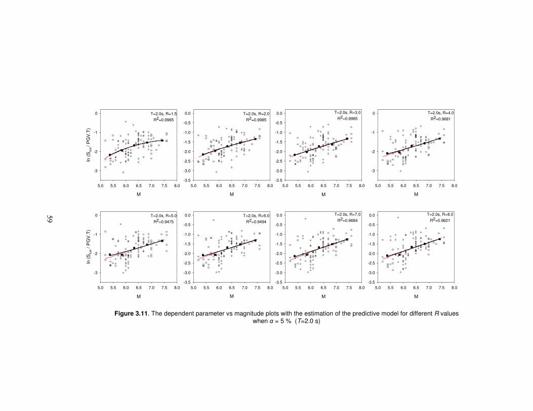
5
9
T=2.0s, R=1.5
R2=0.9965
M
5.0 5.5 6.0 6.5 7.0 7.5 8.0
ln (
Sd,
ie /
PG
V.T
)
-3
-2
-1
0 T=2.0s, R=2.0
R2=0.9985
M
5.0 5.5 6.0 6.5 7.0 7.5 8.0-3.5
-3.0
-2.5
-2.0
-1.5
-1.0
-0.5
0.0 T=2.0s, R=3.0
R2=0.9985
M
5.0 5.5 6.0 6.5 7.0 7.5 8.0-3.5
-3.0
-2.5
-2.0
-1.5
-1.0
-0.5
0.0 T=2.0s, R=4.0
R2=0.9681
M
5.0 5.5 6.0 6.5 7.0 7.5 8.0
-3
-2
-1
0
T=2.0s, R=5.0
R2=0.9475
M
5.0 5.5 6.0 6.5 7.0 7.5 8.0
ln (
Sd,
ie /
PG
V.T
)
-3
-2
-1
0 T=2.0s, R=6.0
R2=0.9494
M
5.0 5.5 6.0 6.5 7.0 7.5 8.0-3.5
-3.0
-2.5
-2.0
-1.5
-1.0
-0.5
0.0 T=2.0s, R=7.0
R2=0.9684
M
5.0 5.5 6.0 6.5 7.0 7.5 8.0-3.5
-3.0
-2.5
-2.0
-1.5
-1.0
-0.5
0.0 T=2.0s, R=8.0
R2=0.9621
M
5.0 5.5 6.0 6.5 7.0 7.5 8.0-3.5
-3.0
-2.5
-2.0
-1.5
-1.0
-0.5
0.0
Figure 3.11. The dependent parameter vs magnitude plots with the estimation of the predictive model for different R values when α = 5 % (T=2.0 s)

6
0
T=0.5s, µ=1.5
R2=0.7636
M
5.0 5.5 6.0 6.5 7.0 7.5 8.0
ln (
Sd,
ie /
PG
V.T
)
-2.5
-2.0
-1.5
-1.0
-0.5
0.0 T=0.5s, µ=2.0
R2=0.7492
M
5.0 5.5 6.0 6.5 7.0 7.5 8.0-2.5
-2.0
-1.5
-1.0
-0.5
0.0 T=0.5s, µ=3.0
R2=0.7202
M
5.0 5.5 6.0 6.5 7.0 7.5 8.0-2.5
-2.0
-1.5
-1.0
-0.5
0.0 T=0.5s, µ=4.0
R2=0.7193
M
5.0 5.5 6.0 6.5 7.0 7.5 8.0-2.5
-2.0
-1.5
-1.0
-0.5
0.0
T=0.5s, µ=5.0
R2=0.7155
M
5.0 5.5 6.0 6.5 7.0 7.5 8.0
ln (
Sd,
ie /
PG
V.T
)
-2.5
-2.0
-1.5
-1.0
-0.5
0.0 T=0.5s, µ=6.0
R2=0.6662
M
5.0 5.5 6.0 6.5 7.0 7.5 8.0-2.0
-1.5
-1.0
-0.5
0.0T=0.5s, µ=7.0
R2=0.7881
M
5.0 5.5 6.0 6.5 7.0 7.5 8.0-2.5
-2.0
-1.5
-1.0
-0.5
0.0T=0.5s, µ=8.0
R2=0.7908
M
5.0 5.5 6.0 6.5 7.0 7.5 8.0-2.5
-2.0
-1.5
-1.0
-0.5
0.0
Figure 3.12. The dependent parameter vs magnitude plots with the estimation of predictive model for different µ values when α = 0 % (T=0.5 s)
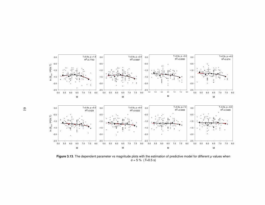
6
1
T=0.5s, µ =1.5
R2=0.7763
M
5.0 5.5 6.0 6.5 7.0 7.5 8.0
ln (
Sd,
ie /
PG
V.T
)
-2.5
-2.0
-1.5
-1.0
-0.5
0.0 T=0.5s, µ =2.0
R2=0.6887
M
5.0 5.5 6.0 6.5 7.0 7.5 8.0-2.5
-2.0
-1.5
-1.0
-0.5
0.0 T=0.5s, µ =3.0
R2=0.6080
M
5.0 5.5 6.0 6.5 7.0 7.5 8.0-2.5
-2.0
-1.5
-1.0
-0.5
0.0 T=0.5s, µ =4.0
R2=0.674
M
5.0 5.5 6.0 6.5 7.0 7.5 8.0-2.5
-2.0
-1.5
-1.0
-0.5
0.0
T=0.5s, µ =5.0
R2=0.629
M
5.0 5.5 6.0 6.5 7.0 7.5 8.0
ln (
Sd,
ie /
PG
V.T
)
-2.5
-2.0
-1.5
-1.0
-0.5
0.0 T=0.5s, µ =6.0
R2=0.6323
M
5.0 5.5 6.0 6.5 7.0 7.5 8.0-2.5
-2.0
-1.5
-1.0
-0.5
0.0T=0.5s, µ=7.0
R2=0.5069
M
5.0 5.5 6.0 6.5 7.0 7.5 8.0-2.5
-2.0
-1.5
-1.0
-0.5
0.0T=0.5s, µ =8.0
R2=0.3489
M
5.0 5.5 6.0 6.5 7.0 7.5 8.0-2.5
-2.0
-1.5
-1.0
-0.5
0.0
Figure 3.13. The dependent parameter vs magnitude plots with the estimation of predictive model for different µ values when α = 5 % (T=0.5 s)
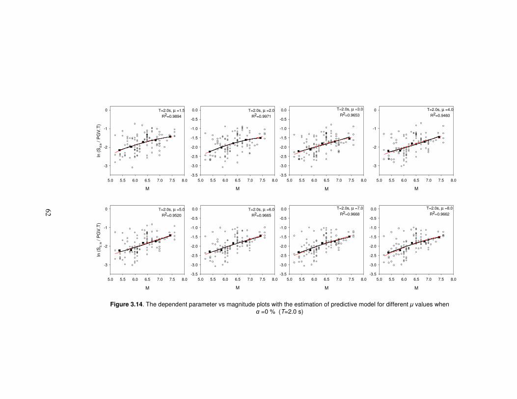
6
2
T=2.0s, µ =1.5
R2=0.9894
M
5.0 5.5 6.0 6.5 7.0 7.5 8.0
ln (
Sd,
ie /
PG
V.T
)
-3
-2
-1
0 T=2.0s, µ =2.0
R2=0.9971
M
5.0 5.5 6.0 6.5 7.0 7.5 8.0-3.5
-3.0
-2.5
-2.0
-1.5
-1.0
-0.5
0.0 T=2.0s, µ =3.0
R2=0.9653
M
5.0 5.5 6.0 6.5 7.0 7.5 8.0-3.5
-3.0
-2.5
-2.0
-1.5
-1.0
-0.5
0.0 T=2.0s, µ =4.0
R2=0.9460
M
5.0 5.5 6.0 6.5 7.0 7.5 8.0
-3
-2
-1
0
T=2.0s, µ =5.0
R2=0.9520
M
5.0 5.5 6.0 6.5 7.0 7.5 8.0
ln (
Sd,
ie /
PG
V.T
)
-3
-2
-1
0 T=2.0s, µ =6.0
R2=0.9665
M
5.0 5.5 6.0 6.5 7.0 7.5 8.0-3.5
-3.0
-2.5
-2.0
-1.5
-1.0
-0.5
0.0 T=2.0s, µ =7.0
R2=0.9668
M
5.0 5.5 6.0 6.5 7.0 7.5 8.0-3.5
-3.0
-2.5
-2.0
-1.5
-1.0
-0.5
0.0 T=2.0s, µ =8.0
R2=0.9662
M
5.0 5.5 6.0 6.5 7.0 7.5 8.0-3.5
-3.0
-2.5
-2.0
-1.5
-1.0
-0.5
0.0
Figure 3.14. The dependent parameter vs magnitude plots with the estimation of predictive model for different µ values when α =0 % (T=2.0 s)

6
3
T=2.0s, µ =1.5
R2=0.990
M
5.0 5.5 6.0 6.5 7.0 7.5 8.0
ln (
Sd,
ie /
PG
V.T
)
-3
-2
-1
0 T=2.0s, µ =2.0
R2=0.9987
M
5.0 5.5 6.0 6.5 7.0 7.5 8.0-3.5
-3.0
-2.5
-2.0
-1.5
-1.0
-0.5
0.0 T=2.0s, µ =3.0
R2=0.9988
M
5.0 5.5 6.0 6.5 7.0 7.5 8.0-3.5
-3.0
-2.5
-2.0
-1.5
-1.0
-0.5
0.0 T=2.0s, µ =4.0
R2=0.9437
M
5.0 5.5 6.0 6.5 7.0 7.5 8.0
-3
-2
-1
0
T=2.0s, µ =5.0
R2=0.9420
M
5.0 5.5 6.0 6.5 7.0 7.5 8.0
ln (
Sd,
ie /
PG
V.T
)
-3
-2
-1
0 T=2.0s, µ =6.0
R2=0.9485
M
5.0 5.5 6.0 6.5 7.0 7.5 8.0-3.5
-3.0
-2.5
-2.0
-1.5
-1.0
-0.5
0.0 T=2.0s, µ =7.0
R2=0.9597
M
5.0 5.5 6.0 6.5 7.0 7.5 8.0-3.5
-3.0
-2.5
-2.0
-1.5
-1.0
-0.5
0.0 T=2.0s,µ =8.0
R2=0.969
M
5.0 5.5 6.0 6.5 7.0 7.5 8.0-3.5
-3.0
-2.5
-2.0
-1.5
-1.0
-0.5
0.0
Figure 3.15. The dependent parameter vs magnitude plots with the estimation of predictive model for different µ values when α =5 % (T=2.0 s)
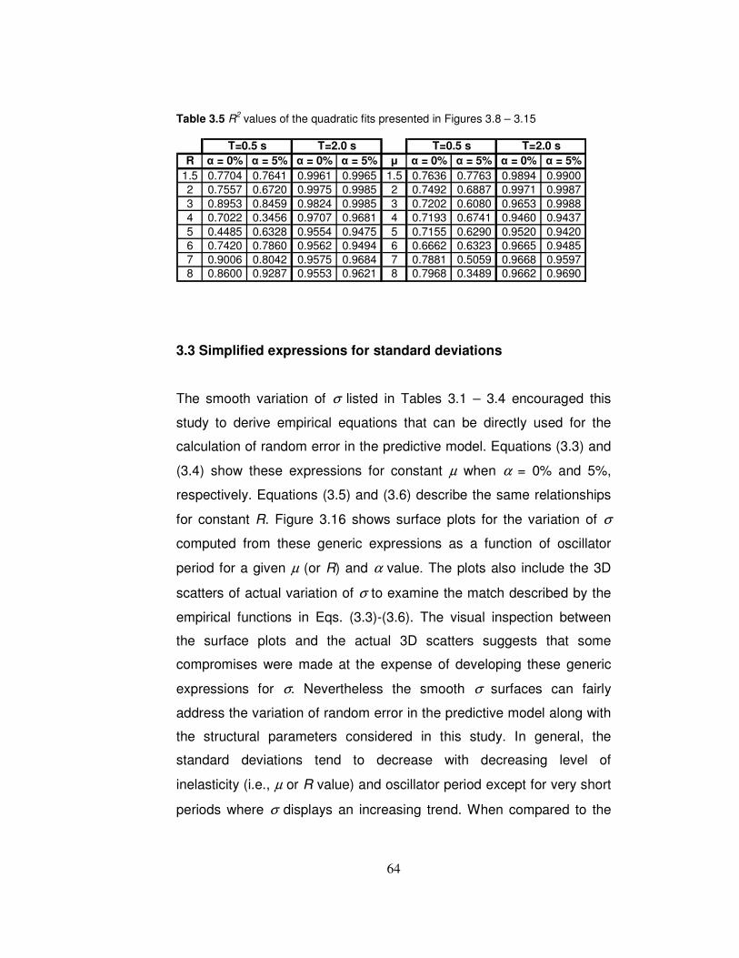
64
Table 3.5 R2 values of the quadratic fits presented in Figures 3.8 – 3.15
R α = 0% α = 5% α = 0% α = 5% µ α = 0% α = 5% α = 0% α = 5%1.5 0.7704 0.7641 0.9961 0.9965 1.5 0.7636 0.7763 0.9894 0.99002 0.7557 0.6720 0.9975 0.9985 2 0.7492 0.6887 0.9971 0.99873 0.8953 0.8459 0.9824 0.9985 3 0.7202 0.6080 0.9653 0.99884 0.7022 0.3456 0.9707 0.9681 4 0.7193 0.6741 0.9460 0.94375 0.4485 0.6328 0.9554 0.9475 5 0.7155 0.6290 0.9520 0.94206 0.7420 0.7860 0.9562 0.9494 6 0.6662 0.6323 0.9665 0.94857 0.9006 0.8042 0.9575 0.9684 7 0.7881 0.5059 0.9668 0.95978 0.8600 0.9287 0.9553 0.9621 8 0.7968 0.3489 0.9662 0.9690
T=0.5 s T=0.5 sT=2.0 s T=2.0 s
3.3 Simplified expressions for standard deviations
The smooth variation of σ listed in Tables 3.1 – 3.4 encouraged this
study to derive empirical equations that can be directly used for the
calculation of random error in the predictive model. Equations (3.3) and
(3.4) show these expressions for constant µ when α = 0% and 5%,
respectively. Equations (3.5) and (3.6) describe the same relationships
for constant R. Figure 3.16 shows surface plots for the variation of σ
computed from these generic expressions as a function of oscillator
period for a given µ (or R) and α value. The plots also include the 3D
scatters of actual variation of σ to examine the match described by the
empirical functions in Eqs. (3.3)-(3.6). The visual inspection between
the surface plots and the actual 3D scatters suggests that some
compromises were made at the expense of developing these generic
expressions for σ. Nevertheless the smooth σ surfaces can fairly
address the variation of random error in the predictive model along with
the structural parameters considered in this study. In general, the
standard deviations tend to decrease with decreasing level of
inelasticity (i.e., µ or R value) and oscillator period except for very short
periods where σ displays an increasing trend. When compared to the

65
constant ductility plots, the constant strength standard deviations are
relatively higher due to the reasoning explained in the previous
paragraph. The standard deviations decrease significantly when α
attains values larger than 0%. The last two observations are consistent
with the previous studies on nonlinear oscillator response (e.g. Ruiz-
García and Miranda, 2003; Chopra and Chintanapakdee, 2004). Note
that the generic expressions derived for σ can be of practical use if the
predictive model is implemented to PSHA together with the GMPEs as
presented in the next section.
( )( ) ( )( ) ( )( )4.0
2
94.057.0 71.001.0
83.008.015.127.0 µµµσ µµµ
TT ++= − (3.3)
( )( ) ( )( ) ( )( )31.0
2
61.045.0 74.001.0
89.0085.009.127.0 µµµσ µµµ
TT ++= − (3.4)
( )( ) ( )( ) ( )( )28.1
2
4.167.0 6.0007.0
035.024.148.4075.011
RT
RTRRRR ++= −−−
σ (3.5)
( )( ) ( )( ) ( )( )87.0
2
32.17.0 66.0008.0
02.092.135.805.011
RT
RTRRRR ++= −−−
σ (3.6)

66
0.0
0.1
0.2
0.3
0.4
0.5
0.6
0.20.4
0.60.8
1.01.2
1.41.6
1.82.0
23
45
67
σ
Period (s)
µ
Constant Ductility - α = 0%
0.0
0.1
0.2
0.3
0.4
0.5
0.6
0.20.4
0.60.8
1.01.2
1.41.6
1.82.0
23
45
67
σ
Period (s)
µ
Constant Ductility - α = 5%
0.0
0.1
0.2
0.3
0.4
0.5
0.6
0.20.4
0.60.8
1.01.2
1.41.6
1.82.0
23
45
67
σ
Period (s)
R
Constant Strength - α = 0%
0.0
0.1
0.2
0.3
0.4
0.5
0.6
0.20.4
0.60.8
1.01.2
1.41.6
1.82.0
23
45
67
σ
Period (s)
R
Constant Strength - α = 5%
Figure 3.16. Smooth variation of standard deviations (σ) derived from Eqs. (3.3) – (3.6) for the predictive model. The scatters are the actual σ presented in Tables 3.1 – 3.4.
3.4 Application of the Proposed Model
The proposed predictive model can estimate the peak inelastic
oscillator displacements for a PGV value that is computed from a
GMPE. Recalling the general functional form of the model in Eq. (3.1)
and applying random variables theory under the assumption that both
PGV and Sd,ie|R,µ are log normal independent variables, one can
incorporate the random error associated with the predicted PGV to the
overall Sd,ie estimation. This is given in Eq. (3.7).

67
( )[ ] ( )[ ] [ ])ln()(lnln,, PGVVarfVarSVar
Ried += θµ
(3.7)
The term on the left hand side of Eq. (3.7) is the total variance of the
peak inelastic oscillator displacement estimation that contains random
error terms due to the predictive model presented and the PGV
estimated from a GMPE (first and second terms on the left hand side,
respectively). Note that the predictive model presented in this study is
derived for random horizontal component definition and this requires a
careful consideration of the GMPE employed for PGV estimation. If the
chosen GMPE is not revised for the random components effect, one
must use a consistent scaling to bring the horizontal component
definition of the chosen GMPE in agreement with the random
component definition used here. Beyer and Bommer (2006) established
empirical relationships between different horizontal component
definitions of PGV for their median estimations and for the associated
random error terms. These relationships can be used efficiently to
obtain compatible and consistent results from the proposed predictive
model when the GMPE considered yields PGV estimations other than
the random horizontal component definition.
Figures 3.17 and 3.18 show the variation in the expected Sd,ie for a set
of constant µ and R values and for reverse style faulting events of
increasing magnitude (M = 5.5, 6.0 and 7.0) at a soft site (NEHRP D)
located 5 km from the surface projection of the fault rupture. Figure 3.17
presents the Sd,ie estimations for α = 0% that can mimic the inelastic
displacement demands on steel frames. Figure 3.18 displays the
expected Sd,ie for α = 5% that fairly represents inelastic concrete
frames. The first column in each figure displays the constant ductility
spectral displacement plots for M = 5.5, 6.0 and 7.0, respectively. The
second column presents the same information for normalized lateral

68
strength spectral displacements. The PGV values of the scenario
events were computed from Akkar and Bommer (2007a) that uses
geometric mean component definition for the estimation of PGV. The
empirical relationships proposed by Beyer and Bommer (2006) were
used to adjust the differences between the random component and
geometric mean definitions. Both figures clearly display the magnitude
influence on the variation of Sd,ie. For small magnitude events (M = 5.5),
the inelastic peak oscillator displacements start oscillating about a
constant plateau after T ≈ 1.5 – 2.0 s. For other magnitude values the
inelastic spectral displacements follow a continuously increasing pattern
with increasing oscillator periods. This observation is consistent with the
previous studies that highlight the strong relationship between
magnitude and spectral corner periods that define the commencement
of constant spectral displacement plateau (e.g. Faccioli et al., 2004;
Bommer and Elnashai, 1999, FEMA, 2003). The PGV dependent
predictive model seems to capture this effect adequately underlining
once again the strong correlation between PGV and magnitude that has
already been addressed by many studies (e.g. Wu et al., 2003; Akkar
and Bommer 2007a). Another common observation from these figures
is that the spectral periods for the commencement of “equal
displacement rule” (i.e. inelastic spectral displacements practically
attaining equal peak displacements of the corresponding elastic
oscillators regardless of the level of inelasticity) are sensitive to the level
of PGV that is essentially related with the magnitude. The increase in
PGV (that is dictated by the increase in magnitude) shifts the spectral
regions towards longer periods where “equal displacement rule” holds.
Tothong and Cornell (2006) while deriving their inelastic spectral
displacement prediction equation also noted this observation.
The influence of postyield stiffness ratio as well as the distinct oscillator
responses imposed by constant µ and R on the peak inelastic oscillator
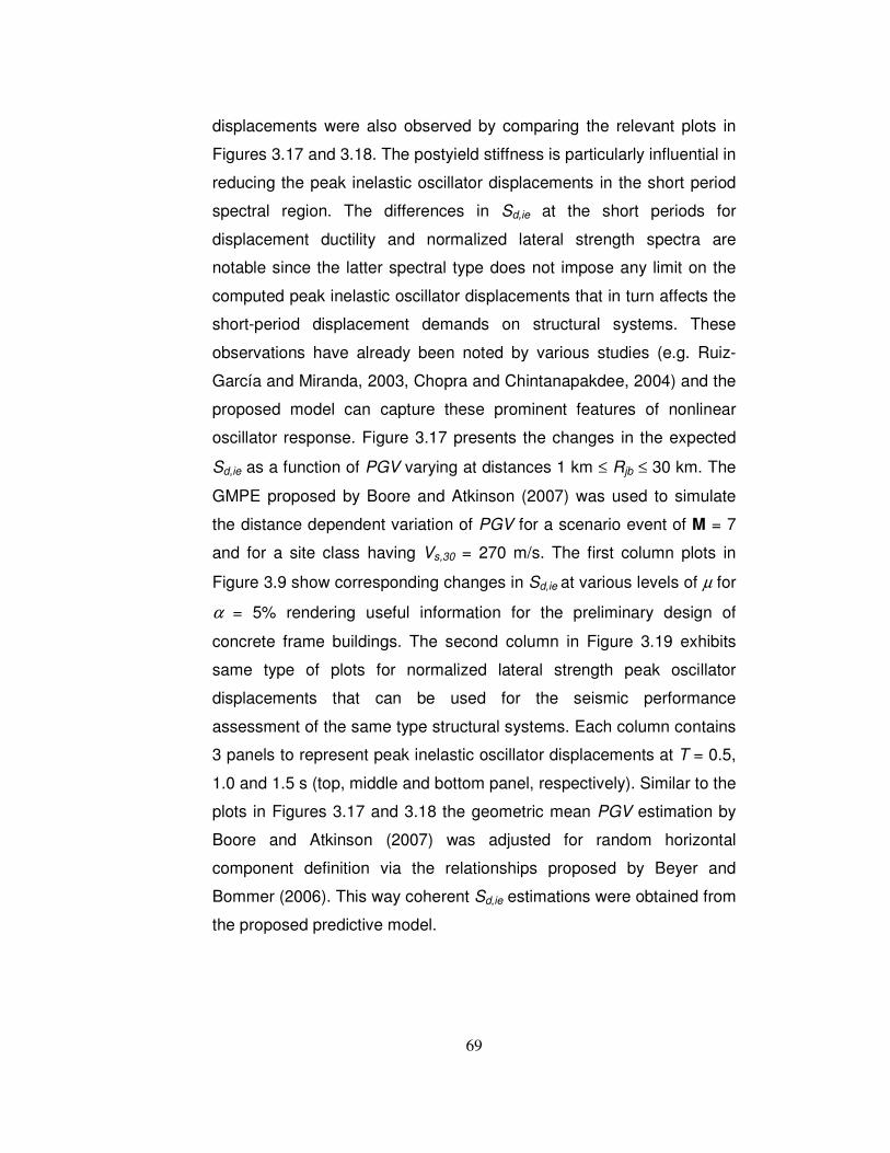
69
displacements were also observed by comparing the relevant plots in
Figures 3.17 and 3.18. The postyield stiffness is particularly influential in
reducing the peak inelastic oscillator displacements in the short period
spectral region. The differences in Sd,ie at the short periods for
displacement ductility and normalized lateral strength spectra are
notable since the latter spectral type does not impose any limit on the
computed peak inelastic oscillator displacements that in turn affects the
short-period displacement demands on structural systems. These
observations have already been noted by various studies (e.g. Ruiz-
García and Miranda, 2003, Chopra and Chintanapakdee, 2004) and the
proposed model can capture these prominent features of nonlinear
oscillator response. Figure 3.17 presents the changes in the expected
Sd,ie as a function of PGV varying at distances 1 km ≤ Rjb ≤ 30 km. The
GMPE proposed by Boore and Atkinson (2007) was used to simulate
the distance dependent variation of PGV for a scenario event of M = 7
and for a site class having Vs,30 = 270 m/s. The first column plots in
Figure 3.9 show corresponding changes in Sd,ie at various levels of µ for
α = 5% rendering useful information for the preliminary design of
concrete frame buildings. The second column in Figure 3.19 exhibits
same type of plots for normalized lateral strength peak oscillator
displacements that can be used for the seismic performance
assessment of the same type structural systems. Each column contains
3 panels to represent peak inelastic oscillator displacements at T = 0.5,
1.0 and 1.5 s (top, middle and bottom panel, respectively). Similar to the
plots in Figures 3.17 and 3.18 the geometric mean PGV estimation by
Boore and Atkinson (2007) was adjusted for random horizontal
component definition via the relationships proposed by Beyer and
Bommer (2006). This way coherent Sd,ie estimations were obtained from
the proposed predictive model.

70
M = 5.5, PGV = 18.3 cm/s
0.1 1
Sd,
ie (
cm)
1
10
M = 6.0, PGV = 29.7 cm/s
0.1 1
Sd,
ie (
cm)
1
10
M = 7.0, PGV = 59.6 cm/s
Period (s)0.1 1
Sd,
ie (
cm)
1
10
µ = 2.0µ = 4.0µ = 6.0µ = 8.0
M = 5.5, PGV = 18.3 cm/s
0.1 1
1
10
M = 6.0, PGV = 29.7 cm/s
0.1 1
1
10
M = 7.0, PGV = 59.6 cm/s
Period (s)0.1 1
1
10
R = 2.0R = 4.0R = 6.0R = 8.0
Figure 3.17. Inelastic spectral displacement estimations of the proposed predictive model for constant µ (first column) and constant R (second column) as a function of magnitude when α = 0%.

71
M = 5.5, PGV = 18.3 cm/s
0.1 1
Sd,
ie (
cm)
1
10
M = 6.0, PGV = 29.7 cm/s
0.1 1
Sd,
ie (
cm)
1
10
M = 7.0, PGV = 59.6 cm/s
Period (s)0.1 1
Sd,
ie (
cm)
1
10
µ = 2.0µ = 4.0µ = 6.0µ = 8.0
M = 5.5, PGV = 18.3 cm/s
0.1 1
1
10
M = 6.0, PGV = 29.7 cm/s
0.1 1
1
10
M = 7.0, PGV = 59.6 cm/s
Period (s)0.1 1
1
10
R = 2.0R = 4.0R = 6.0R = 8.0
Figure 3.18. Inelastic spectral displacement estimations of the proposed predictive model for constant µ (upper row) and constant R (lower row) as a function of magnitude when α = 5%.
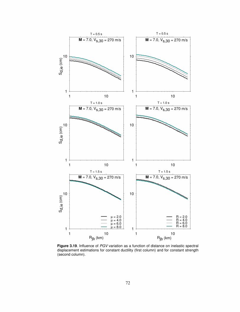
72
M = 7.0, Vs,30 = 270 m/s
1 10
Sd,
ie (
cm)
1
10
M = 7.0, Vs,30 = 270 m/s
1 10
Sd,
ie (
cm)
1
10
M = 7.0, Vs,30 = 270 m/s
1 10
Sd,
ie (
cm)
1
10
µ = 2.0µ = 4.0µ = 6.0µ = 8.0
M = 7.0, Vs,30 = 270 m/s
1 101
10
M = 7.0, Vs,30 = 270 m/s
1 101
10
M = 7.0, Vs,30 = 270 m/s
Rjb (km)1 10
1
10
R = 2.0R = 4.0R = 6.0R = 8.0
T = 1.0 s
T = 0.5 s
T = 1.5 s
T = 1.0 s
T = 0.5 s
T = 1.5 s
Rjb (km) Figure 3.19. Influence of PGV variation as a function of distance on inelastic spectral displacement estimations for constant ductility (first column) and for constant strength (second column).

73
The plots consistently show that the distance dependent decay in PGV
results in a decrease in Sd,ie estimations. For short-period systems the
change in PGV as a function of distance has more prominent influence
at different levels of inelasticity that are described by various values of µ
and R. This influence diminishes gradually as the structural period shifts
to longer periods and it is almost invisible after T = 1.5 s for the
particular α value used. The reason behind this observation can be
related to the postyield stiffness ratio, the rate of change in distance-
dependent PGV variation and the magnitude-dependent corner periods
that define either the equal displacement spectral ranges or the
constant displacement spectral plateau. The proposed model can fairly
account for these seismological parameters that play important role on
the peak inelastic oscillator displacements.

74
CHAPTER 4
CONCLUDING REMARKS
4.1 General
The main objective of this study is to propose a model to estimate the
nonlinear peak oscillator deformation demands as a function of peak
ground velocity (PGV) which is a promising ground-motion intensity
measure having a strong relationship with earthquake magnitude. The
predictive model considers the random error term that is a function of
period (T) and displacement ductility (µ) or normalized lateral strength
ratio (R).
The secondary objective of this study is to observe the relationships
between some of the ground-motion intensity measures (PGA, PGV
and PSa(T1)) and the global deformation demands of multi-degree-of
freedom systems (i.e. maximum interstory drift ratio, MIDR and
maximum roof drift ratio, MRDR). This way the study compares and
verifies the observations of Akkar and Özen (2005) that are validated
only for single-degree-of-freedom systems.
As a part of this thesis, recently developed ground-motion prediction
equations (GMPE) for PGV by Akkar and Bommer (2007a) and Boore
and Atkinson (2007) are used for displaying the practicality and
applicability of the proposed model via GMPEs.
75
4.2 Summary and Conclusions of Chapter 2
Chapter 2 includes information about the ground-motion records and
modeling and design of buildings used in this study. The important
seismological features of the records and the detailed dimensioning of
the structural members in the building models are also presented. The
results of response history analyses (RHA) for building models as well
as the specific conditions and assumptions taken into account in the
RHA are provided within the context of this chapter.
The study has made use of two sets of ground-motion records of
moderate-to large-events recorded on site classes NEHRP C and
NEHRP D. None of the sets contains dominant pulse signals. The first
set is composed of 60 ground-motion records and it is used to
investigate the relationship between some of the ground-moton intensity
indices and the global deformation demands of MDOF models with 3, 5,
7 and 9 stories. This set is divided into 3 bins each having 20 records
according to the PGV values. The PGV range of first bin records is 1
cm/s < PGV < 20 cm/s wheras the PGV ranges of second and third bins
are 20 cm/s < PGV < 40 cm/s and 40 cm/s < PGV < 60 cm/s,
respectively. The second set is comprised of 109 records in total; 54 of
which is from the European ground-motion dataset compiled by Akkar
and Bommer (2007) and the rest is from the first set. The second data
set describes the random component effect.
Five different building models (e1, e2, e3, e1’ and e2’) of different
number of stories (i.e. 3, 5, 7 and 9 story) are designed from three
different median design spectra assembled according to the above sub-
bins of first ground-motion dataset. e1, e2 and e3 models are designed
according to median spectra of the first, second and third bin,
respectively. The e1’ and e2’ models preserve the size and dimensions

76
of e1 and e2 models, respectively. Their reinforcement are calculated
according to the design spectrum of the third bin. The nonlinear time
history and pushover analyses of the models are conducted by using
the IDARC-2D structural analysis software under three different
structural behaviors: non degrading, stiffness degrading and stiffness
and strength degrading, respectively. MRDR and MIDR values are
taken as the global deformation demand measures for MDOF systems
and the relationships between these demand measures and intensity
measures (PGA, PGV and PSa(T1)) are investigated and evaluated
through Spearman’s correlation coefficient (ρ) .
The most important observations obtained from this chapter are listed
below:
• Pushover curves idealized according to ATC-40 reveal good
agreement with the absolute maximum roof displacement versus
base shear plots that are obtained from RHA. The pushover
curves are computed using the inverted triangular loading pattern
and the above match between the pushover curves and RHA
results verify the first-mode dominant behavior of the models.
• The ρ values tend to increase for PGV vs. MRDR and PGV vs.
MIDR scatters with increasing story number in all three hysteretic
behaviors. This observation advocates that PGV corelates well
with the global deformation demands with increasing story
number. There is no clear relationship between the increase in
story number and the associated ρ values for PGA vs. MRDR
and PGA vs. MIDR. In the case of PSa(T1) vs. MRDR and
PSa(T1) vs. MIDR a trend that is similar to the one observed in
PGV is identified. However, the associated ρ values of PSa(T1)
are smaller than those of PGV.

77
• The comparisons between the ρ values of all ground-motion
intensity measures reveal that regardless of the hysteretic
behaviors investigated the highest ρ values are the ones
associated with PGV.
• An observation valid for all hysteretic behaviors and for all
ground-motion intensity measures is that the associated ρ values
of MRDR are higher than those of MIDR for 3 and 9 story models
while for 5 and 7 stories ρ values of MIDR is higher with few
exceptions.
4.3 Summary and Conclusions of Chapter 3
This chapter presents a predictive model for estimating the constant
ductility (µ) and normalized lateral strength (R) spectral displacements
for a given initial period, magnitude and PGV value. Sensitivity analysis
that considered the influence of ground-motion parameters such as
magnitude, distance, site class etc. on the dimensionless predictive
parameter Sd,e / (PGVxT) is conducted to use it in the predictive model.
The proposed model also accounts for the random error by the
empirical equations that are function of R (or µ) and T. In order to
demonstrate the use of the predictive model with ground-motion
prediction equations, case studies are provided in the last section of this
chapter under different scenarios. Major observations obtained from this
chapter are listed below:
• Sensitivity analyses conducted using the ground-motion
prediction equations of Akkar and Bommer (2007a, 2007b) and
Boore and Atkinson (2007) showed that magnitude influence on
the predicted parameter is considerably high when compared to

78
the influence of distance. The investigation on the effect of
faulting style on the predicted parameter revealed that style of
faulting is not as influential as magnitude.
• As for the effect of site class on the predicted parameter
Sd,e / (PGVxT) a departure between soft and stiff site is observed
for large magnitude and mid-period values while there is no clear
difference for low-period values in the curves of stiff and soft
sites.
• The assumption of the regression method used (Least Squares
Regression) that dictates normal distribution for random error
terms with zero mean and σ2 is satisfied by the normal probability
plots of the residuals. As a matter of fact, it can be concluded
that aleatory uncertainty associated with the predictive model
can be fairly explained well by the variances computed from the
residual mean squares.
• When the residual plots of the model as a function magnitude are
considered, the associated dispersion is relatively higher in
α=0% than in α=5%. However, in both cases the plots do not
exhibit a biased trend in the residuals.
• The variation of standard deviations shows that the σ values
decrease with increasing α value and with decreasing level of
inelasticity.
• The Sd,ie vs. period plots obtained from the application of the
proposed model revealed that the increase in PGV shifts spectral
regions towards longer periods.

79
• At short period ranges, the difference between Sd,ie values of
ductility and normalized lateral strength are notable.
• Sd,ie vs. Rjb plots showed that distance dependent decrease in
PGV values resulted in a decrease in Sd,ie estimations especially
for short periods.
It is concluded that the predictive model is adequate in differentiating
the difference in nonlinear oscillator response imposed by the constant
ductility and normalized lateral strength ratio. These features make the
predictive model versatile for preliminary design and seismic
performance of a broad class of building systems.
4.4 Recommendations for Further Studies
The following issues can be addressed in a broader sense in further
studies:
• The proposed model is developed from a limited number of
ground-motion records. The model can be improved by adding
more records in the regression analyses stage to account for a
wide range of ground motion features inherited in the records.
• More complex predictive models can be developed by
considering the influence of independent ground-motion
parameter (style of faulting, site class, distance etc.) other than
magnitude. Similar models can be obtained for a specific style of
faulting or site classes using the specifically selected ground
motion records.

80
• Expressions that calculate the random error can be investigated
further by considering the magnitude influence.
• The compatibility of the proposed model with ground motion
prediction equations for PGV other than Akkar and Bommer
(2007a) and Boore and Atkinson (2007) can be investigated.

81
REFERENCES
Akkar S, Bommer J.J., Empirical prediction equations for peak ground velocity derived from strongmotion records from Europe and the Middle East, Bulletin of the Seismological Society of America 2007a; 97(2): 511-530. Akkar S, Bommer J.J., Prediction of elastic displacement response spectra in Europe and the Middle East, Earthquake Engineering and Structural Dynamics 2007b; 36: 1275-1301. Akkar S, Bommer JJ., Influence of long-period filter cut-off on elastic spectral displacements, Earthquake Engineering and Structural Dynamics 2006; 35(9): 1145-1165. Akkar S, Özen, Ö., Effect of peak ground velocity on deformation demands for SDOF systems, Earthquake Engineering and Structural Dynamics 2005; 34(13): 1551-1571. Akkar S., Sucuoğlu H and Yakut A., Displacement-based fragility functions for low- and mid-rise ordinary concrete buildings, Earthquake Spectra, 2005; 21(4): 901-927. Arroyo D, Terán A., Strength reduction factors for ductile structures with passive energy dissipating devices, Journal of Earthquake Engineering; 2003 7(2): 297-325. ASCE., Prestandard and commentary for the seismic rehabilitation of buildings, Report No. FEMA 356, American Society of Civil Engineers, Washington DC, 2000. ATC, Improvement of nonlinear static seismic analysis procedures. Report No. FEMA 440, Applied Technology Council, Washington DC, 2005. Atkinson, G. M. and Boore, D. M., Ground-motion relations for eastern North America, Bulletin of the Seismological Society of America 85(1), 17–30,1995 Baéz J.I, Miranda E., Amplification factors to estimate inelastic displacement demands for the design of structures in the near field, Proceedings of 12th World Conference on Earthquake Engineering, CDRom Auckland, New Zealand, 2000.

82
Beyer K, Bommer J.J., Relationships between median values and between aleatory variabilities for different definitions of the horizontal component of motion, Bulletin of the Seismological Society of America 2006; 96(4A):1512-1522. Bommer J.J, Stafford P.J, Alarcón J.E. and Akkar S., Ground-motion predictions over extended magnitude range, Bulletin of the Seismological Society of America 2007, in press. Bommer J.J, Elnashai A.S., Displacement spectra for seismic design,. Journal of Earthquake Engineering 1999; 3(1):1-32. Boore D.M, Atkinson G., Ground-Motion Predictions Equations for the Average Horizontal Component of PGA, PGV, and 5%-Damped SA at Spectral Periods between 0.01 s and 10.0, Submitted for publication in Earthquake Spectra, 2007. Bray J.D, Rodriguez-Marek A., Characterization of forward-directivity ground motions in the near-fault region, Soil Dynamics and Earthquake Engineering 2004; 24(11): 815-828. Campbell, K. W., Empirical near-source attenuation relationships for horizontal and vertical components of peak ground acceleration, peak ground velocity, and pseudo-absolute acceleration response spectra, Seismological Research Letters 68(1), 154–179, 1997 Chakraborati A, Gupta V.K., Scaling of strength reduction factors for degrading elasto-plastic oscillators, Earthquake Engineering and Structural Dynamics 2005; 34:189–206. Chopra A.K, Chintanapakdee C., Comparing response of SDF systems to near-fault and far-fault earthquake motions in the context of spectral regions, Earthquake Engineering and Structural Dynamics 2001; 30:1769–1789.
Chopra A.K, Chintanapakdee C., Inelastic Deformation Ratios for Design and Evaluation of Structures: Single-Degree-of-Freedom Bilinear Systems, Journal of Structural Engineering 2004; 130:1309-1319. Cuesta I, Aschheim M.A, Fajfar P., Simplified R-Factor Relationships for Strong Ground Motions, Earthquake Spectra 2003; 19(1):25-45. Douglas J, Smit P.M., How Accurate Can Strong Ground Motion Attenuation Relations Be?, Bulletin of the Seismological Society of America 2001; 91(6): 1917-1923.

83
Draper N.R, Smith H., Applied Regression Analysis, Second edition, John Wiley & Sons Inc., New York, 709 pp, 1981. Douglas, J., Earthquake ground motion estimation using strong-motion records:A review of equations for the estimation of peak ground accelerations and response spectral ordinates, Earth-Science Reviews 61, 43-104, 2003 Elghadamsi F, Mohraz B., Inelastic earthquake spectra, Earthquake Engineering and Structural Dynamics 1987; 15:91–104. Faccioli E, Paolucci R, Rey J., Displacement spectra for long periods, Earthquake Spectra 2004; 20(2):347-376. Fajfar, P., Vidic, T., and Fischinger., M., A measure of earthquake motion capacity to damage medium-period structures, Soil Dynamics and Earthquake Engineering,1990, 9(5), 236–242. Farrow K.T, Kurama A., SDOF demand index relationships for performance-based seismic design, Earthquake Spectra,1998; 19:799-838 FEMA, NEHRP guidelines for the seismic rehabilitation of buildings. Guidelines (FEMA 273) and Commentary (FEMA-274), Federal Emergency Management Agency, Washington DC, 1997. FEMA, The 2003 NEHRP recommended provisions for new buildings and other structures. Part 1: Provisions (FEMA 450), Federal Emergency Management Agency, Washington DC, 2003. Frisenda, M., Massa, M., Spallarossa, D., Ferretti, G. and Eva, C., Attenuation relationships for low magnitude earthquakes using standard seismometric records, Journal of Earthquake Engineering 9(1), 23–40, 2005 Gregor, N., Silva, W. and Darragh, B., Development of attenuation relations forpeak particle velocity and displacement, Pearl Report to PG&E/CEC/Caltrans/Pacific Engineering and Analysis, Retrieved from http://www. pacificengineering.org/rpts page1.html on February 12, 2002 Joyner W.B, Boore D.M., Peak horizontal acceleration and velocity from strong-motion records including records from the 1979 Imperial Valley, California, earthquake, Bulletin of the Seismological Society of America 1981; 71(6): 2011-2038.

84
Karmakar D, Gupta V.K., Estimation of strength reduction factors via normalized pseudo-acceleration response spectrum, Earthquake Engineering and Structural Dynamics 2007; 36:751–763. Kramer, S.L, Geotechnical Earthquake Engineering, Prentice Hall, New Jersey, 1996 Krawinkler, Challenges and Progress in Performance-based Earthquake Engineering, International Seminar on Seismic Engineering for Tomorrow – In Honor of Professor Hiroshi Akiyama Tokyo, Japan, November 26, 1999 Kurama Y.C, Farrow K.T, Ground motion scaling methods for different site conditions and structure characteristics, Earthquake Engineering and Structural Dynamics, 2003; 32 (15): 2423–2450. MacRae G.A, Tagava H., Methods to estimate displacements of PG&E structures, Final Report PG&E/PEER Task No. 505, Seattle Washington, 2002. MacRae G.A, Morrow D.V, Roeder C.W, Near-fault ground motion effects on simple structures, Journal of Structural Engineering, 2001; 127(9): 996-1004. MacRae G.A, Roeder C.W, Near-field ground motion effects on short structures, Final Report to PG&E/PEER, Pacific Earthquake Engineering Research Center, Richmond, CA, 1999. Mahin S.A., Bertero V.V, An evaluation of inelastic seismic design spectra, Journal of Structural Division, 1981; 107: 1777-1795. Metin,A., Inelastic deformation demands on moment-resisting frame structures, M.S Dissertation, METU,Ankara, 2006 Miranda E., Inelastic displacement ratios for structures on firm sites, Journal of Structural Engineering, 2000; 126:1150-1159. Miranda E., Bertero V.V., Evaluation of strength reduction factors for earthquake-resistant design, Earthquake Spectra, 1994; 10(2), 357–397.
Miranda E., Site dependent strength reduction factors, Journal of Structural Engineering 1993; 119: 3503-3519.

85
Miranda E, Estimation of inelastic deformation demands of SDOF systems, Journal of Structural Engineering (ASCE) 2001;127 (9):105-112 Molas, G. L. and Yamazaki, F., Attenuation of response spectra in Japan using new JMA records, Bulletin of Earthquake Resistant Structures ,1996, 29, 115–128. Myers R.H., Classical and modern regression with applications, PWS Publishers, Boston Massachusetts, 359 pp, 1986. Nassar A.A, Krawinkler H., Seismic Demands for SDOF and MDOF Systems. Report No. 95, The John A. Blume Earthquake Engineering Center, Stanford University, CA, 1991. Newmark N.M, Hall W.J., Seismic Design Criteria for Nuclear Reactor Facilities, Report No. 46, Building Practices for Disaster Mitigation, National Bureau of Standards, U.S. Department of Commerce, 209-236, 1973. Newmark N.M, Hall W.J., Earthquake Spectra and Design. EERI Monograph Series, Earthquake Engineering Research Institute, Oakland, CA, 1982. Ordaz M, Pérez-Rocha L.E., Estimation of strength-reduction factors for elasto-plastic systems: A new approach, Earthquake Engineering and Structural Dynamics 1998; 27:889–901. Pankow, K. L. and Pechmann, J. C., The SEA99 ground-motion predictive relations and new peak ground velocity relation, Bulletin of the Seismological Society of America, 2004, 94(1), 341–348. Press W.H, Flannery B.P, Teukolsky S.A and Vetterling W.T., Numerical recipes: the art of scientific computation (FORTRAN version), Cambridge University Press, Cambridge, 702 pp, 1989. Riddell R., On ground motion intensity indices, Earthquake Spectra, 2007; 23(1): 147-173. Riddell R, Garcia J.E, Garces E., Inelastic deformation response of SDOF systems subjected to earthquakes, Earthquake Engineering and Structural Dynamics, 2002; 31:515-538. Ruiz García J, Miranda E., Inelastic ratios for design of structures on soft soils sites, Journal of Structural Engineering, 2004; 130(12): 2051-2061.

86
Ruiz-García J, Miranda E., Inelastic displacement ratios for evaluation of existing structures, Earthquake Engineering and Structural Dynamics 2003; 32:1237-1258. Sadigh, R. K. and Egan, J. A., Updated relationships for horizontal peak ground velocity and peak ground displacements for shallow crustal earthquakes, Proceedings of the Sixth US National Conference on Earthquake Engineering, Seattle, Paper No. 317, 1998 Sewel R.T., Damage effectiveness of earthquake ground motion: characterizations based on the performance of structures and equipment, PhD Thesis, Department of Civil and Environmental Engineering, Stanford University, Stanford CA., 619 pp., 1989. Singh, S.K., Gansl, B.K., Bhattacharya, S.N., Pacheco, J.F., Dattatrayam, R.S., Ordaz, M., Kamal, G.S. and Hough, S.E., Estimation of ground motion for Bhuj (26 January 2001; Mw 7.6) and for future earthquakes in India, Bulletin of Seismological Society of America, 2003, 93(1), 353–370. Sucuoğlu H., Yazgan U., and Yakut A., A Screening Procedure for Seismic Risk Assessment in Urban Building Stocks, Earthquake Spectra, 2007; 23(2): 441-458. Tothong P., Cornell A.C., An empirical ground-motion attenuation relation for inelastic spectral displacement, Bulletin of the Seismological Society of America 2006; 96(6): 2146-2164. Tromans, I. J. and Bommer, J. J., The attenuation of strong-motion peaks in Europe, Proceedings of the Twelfth European Conference on Earthquake Engineering, London, Paper 394, 2002 Valles, R.E., Reinhorn, A.M., Kunnath, S.K., Li, C., and Madan, A., IDARC-2D: A program for the inelastic damage analysis of buildings,, National Center for Earthquake Engineering Research, State University of New York at Buffalo, 1996 Veletsos A.S., Newmark N.M., Effect of inelastic behavior on the response of simple systems to earthquake motions, Proceedings of 2nd World Conf. on Earthquake Engineering, Vol. II, Tokyo, 895–912., 1960. Vidic T., Fajfar P., Fischinger M., Consistent inelastic design spectra: strength and displacement, Earthquake Engineering and Structural Dynamics 1994; 23:507–521.

87
Yılmaz, H., Correlation of deformation demands with ground motion intensity, M.S Dissertation, METU, Ankara, 2007 Wu Y.M, Teng TI, Shin T.C, Hsiao N.C., Relationship between peak ground acceleration, peak ground velocity and intensity in Taiwan. Bulletin of the Seismological Society of America 2003; 93:386-396.

88
APPENDIX A
MDOF MODELS
A.1. General
Four different story reinforced concrete models are employed in this
study depicting the low to mid rise building stock of general construction
practice in Turkey as 3, 5, 7 and 9 stories respectively. Each model
further divided into 5 subgroups. The subgroups are based on the
design spectra used. Five subgroups can be listed as follows:
• e1 - Models are designed using the design spectrum obtained
from the Bin 1 (0 cm/s < PGV<20 cm/s)
• e2 - Models are designed using the design spectrum obtained
from the Bin 2 (20 cm/s < PGV<40 cm/s)
• e3 - Models are designed using the design spectrum obtained
from the Bin 3 (40 cm/s < PGV<60 cm/s)
• e1' – The reinforcement detailing of e1 models are redesigned
using the response spectrum of Bin 3
• e2' – The reinforcement detailing of e2 models are redesigned
using the response spectrum of Bin 3
The reinforcement designs of the models are conducted by SAP 2000
v.8.2.3. The values on the stress-strain curves of steel and concrete are
calculated as suggested by IDARC-2D after the decision of the
compressive strength of the materials (Figure A.1 and A.2), (Valles et
al, 1996).

89
Concrete
Figure A.1 Stress- strain curve of concrete
FC : Unconfined compressive strength - 20 MPa
EC : Initial young’s modulus - 26800
EPSO :Strength at max. Strength of concrete - 0.2%
FT : Stress at tension cracking - 2.4 MPa
EPSU : Ultimate strain in compression (%) - 0 %
ZF : Parameter defining slop of falling branch - 0
Reinforcement
Figure A.2 Stress- strain curve of steel

90
FS:Yield strength - 420 MPa
FSU : Ultimate strength - 588 MPa
ES : Modulus of elasticity - 200000
ESH : Modulus of strain hardening - 3333
EPSH : Strain at start of hardening (%) - 3.0 %
FSU =1.4*FS ESH = (ES/60) ksi EPSH=3 % During the column and beam design the following values are taken for
the members. Well confinement is selected for the members, which
reflects the effectiveness of the confinement (Figure A.3). The
corresponding values are taken for rigid zone length, hoop bar diameter
and spacing, diameter and spacing of stirrups, distance from centroid to
cover as shown in Table A.1.
Figure A.3. Confinement effectiveness (Valles et al, 1996)
Table A.1 Some specific distances used in the design of members Distances used in design of members Beam Column Distances used in design of members Beam Column
Rigid zone length (cm) 22.5 25 Cover to centroid of the steel (cm) 5 -
Distance from centroid Effective slab width (cm) 30 -
of reinf. to face of column (cm) - 6.5 Slab Thickness (cm) 0 -
Hoop bar diameter (cm) - 1.2 Diameter of stirrups (cm) 1 -
Hoop bar spacing (cm) - 7.5 Spacing of stirrups (cm) 13.5 -

91
A.2 Model 3e1
Figure A.4 Reinforcement areas in cm2 for 3e1
A.3 Model 3e2
Figure A.5 Reinforcement areas in cm2 for 3e2

92
A.4 Model 3e3
Figure A.6 Reinforcement areas in cm2 for 3e3
A.5 Model 3e1'
Figure A.7 Reinforcement areas in cm2 for 3e1'
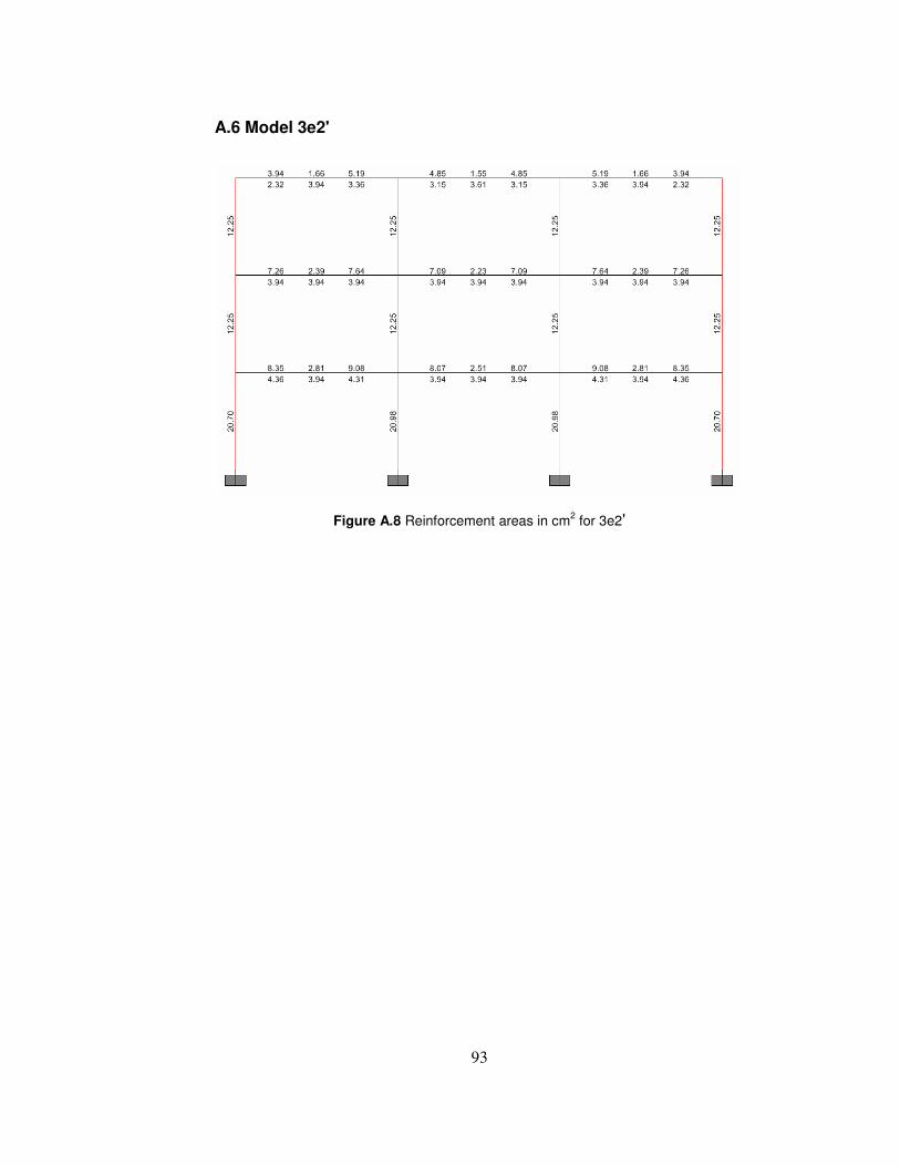
93
A.6 Model 3e2'
Figure A.8 Reinforcement areas in cm2 for 3e2'

94
A.7 Model 5e1
Figure A.9 Reinforcement areas in cm2 for 5e1

95
A.8 Model 5e2
Figure A.10 Reinforcement areas in cm2 for 5e2

96
A.9 Model 5e3
Figure A.11 Reinforcement areas in cm2 for 5e3

97
A.10 Model 5e1'
Figure A.12 Reinforcement areas in cm2 for 5e1'

98
A.11 Model 5e2'
Figure A.13 Reinforcement areas in cm2 for 5e2'

99
A.12 Model 7e1
Figure A.14 Reinforcement areas in cm2 for 7e1
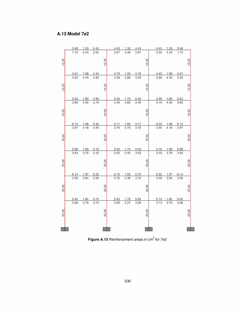
100
A.13 Model 7e2
Figure A.15 Reinforcement areas in cm2 for 7e2
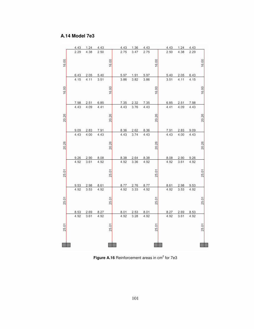
101
A.14 Model 7e3
Figure A.16 Reinforcement areas in cm2 for 7e3

102
A.15 Model 7e1'
Figure A.17 Reinforcement areas in cm2 for 7e1'

103
A.16 Model 7e2'
Figure A.18 Reinforcement areas in cm2 for 7e2'
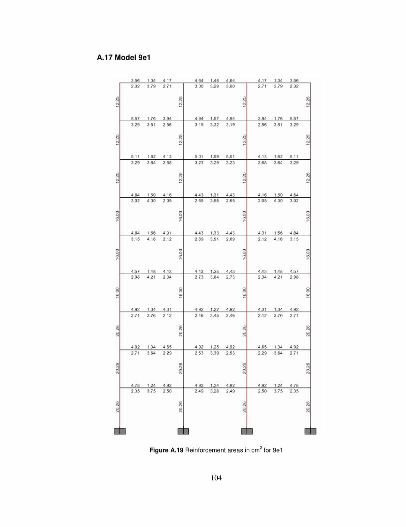
104
A.17 Model 9e1
Figure A.19 Reinforcement areas in cm2 for 9e1

105
A.18 Model 9e2
Figure A.20 Reinforcement areas in cm2 for 9e2

106
A.19 Model 9e3
Figure A.21 Reinforcement areas in cm2 for 9e3
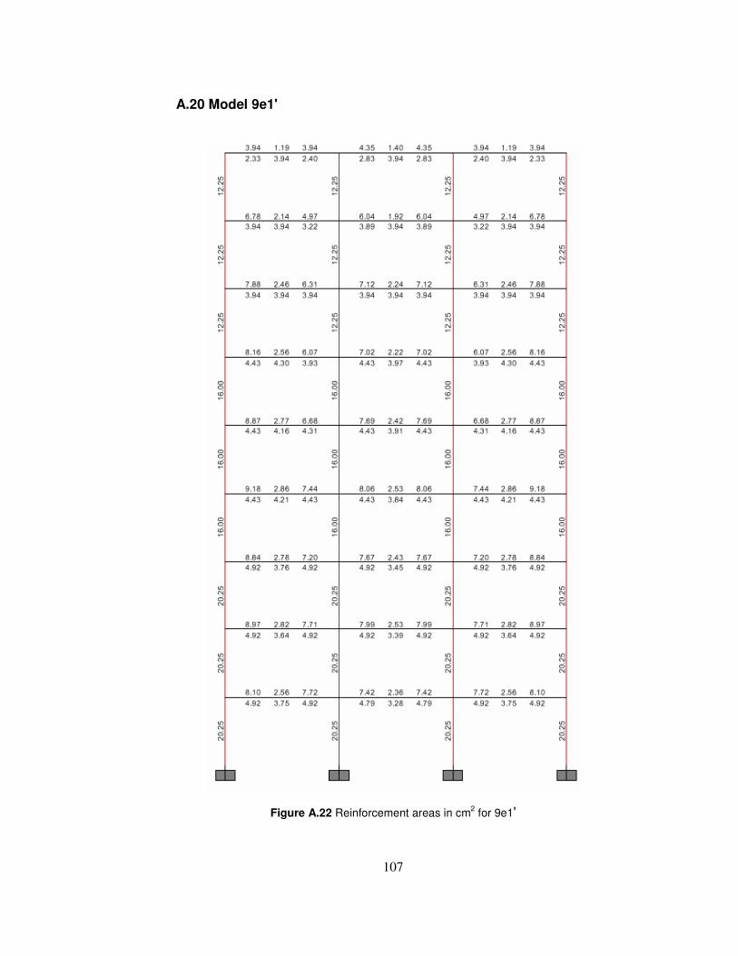
107
A.20 Model 9e1'
Figure A.22 Reinforcement areas in cm2 for 9e1'

108
A.21 Model 9e2'
Figure A.23 Reinforcement areas in cm2 for 9e2'

109
Story Mode Σ mass T(s) ΓΓΓΓ ΦΦΦΦ % weight T(s) ΓΓΓΓ ΦΦΦΦ % weight
3 1 0.674 0.809 1.560 86.658 0.567 0.809 1.556 86.623
(133t) 2 0.220 0.280 -1.236 10.377 0.177 0.283 -1.223 10.568
3 0.130 0.150 0.559 2.966 0.102 0.146 0.597 2.809
5 1 1.016 1.025 1.275 82.190 0.779 1.029 1.265 82.845
(224t) 2 0.347 0.375 -1.188 10.991 0.262 0.371 -1.178 10.794
3 0.192 0.219 0.967 3.748 0.144 0.217 0.964 3.693
4 0.136 0.160 -0.537 2.010 0.101 0.149 -0.583 1.739
5 0.097 0.116 0.110 1.061 0.072 0.109 0.128 0.929
7 1 1.140 1.195 1.139 79.313 0.951 1.189 1.130 78.625
(315t) 2 0.421 0.455 -1.168 11.531 0.339 0.474 -1.081 12.496
3 0.243 0.286 0.908 4.559 0.193 -0.273 -0.959 4.150
4 0.165 0.171 -0.804 1.621 0.128 -0.184 0.824 1.872
5 0.126 0.167 0.361 1.550 0.098 0.161 0.460 1.439
6 0.097 0.124 -0.102 0.855 0.075 0.124 -0.140 0.852
7 0.071 0.101 0.010 0.570 0.054 0.101 0.014 0.567
9 1 1.283 1.330 1.034 76.168 1.113 1.353 0.988 78.912
(407t) 2 0.474 0.545 -1.031 12.786 0.389 0.504 -1.011 10.944
3 0.272 0.348 0.861 5.229 0.220 0.320 0.886 4.419
4 0.185 0.212 -0.867 1.932 0.148 0.217 -0.857 2.022
5 0.135 -0.183 -0.619 1.442 0.108 -0.181 -0.652 1.411
6 0.106 -0.135 0.480 0.787 0.082 -0.141 0.502 0.858
7 0.088 -0.139 -0.182 0.838 0.068 0.120 0.275 0.619
8 0.070 -0.096 0.042 0.395 0.054 0.099 -0.064 0.420
9 0.054 0.099 0.425 0.043 0.096 0.394
e1' e2'
Story Mode
Σ mass T(s) ΓΓΓΓ ΦΦΦΦ % weight T(s) ΓΓΓΓ ΦΦΦΦ % weight T(s) ΓΓΓΓ ΦΦΦΦ % weight
3 1 0.733 0.820 1.517 89.062 0.586 0.816 1.537 88.029 0.412 0.805 1.578 85.805
(133t) 2 0.235 0.263 -1.231 9.135 0.182 0.272 -1.228 9.811 0.122 0.291 -1.215 11.222
3 0.141 0.117 0.676 1.802 0.104 0.128 0.636 2.160 0.063 0.150 0.555 2.973
5 1 1.043 1.029 1.268 82.959 0.787 1.031 1.261 83.134 0.698 1.025 1.267 82.310
(224t) 2 0.357 0.373 -1.177 10.877 0.264 0.370 -1.177 10.720 0.226 0.371 -1.196 10.770
3 0.197 0.212 0.976 3.528 0.145 0.216 0.964 3.645 0.121 0.228 0.946 4.069
4 0.142 0.150 -0.563 1.759 0.102 0.145 -0.593 1.656 0.080 0.157 -0.565 1.924
5 0.099 0.106 0.106 0.877 0.073 0.104 0.133 0.845 0.056 0.109 0.156 0.928
7 1 1.152 1.194 1.139 79.307 0.958 1.189 1.129 78.642 0.872 1.189 1.123 78.530
(315t) 2 0.425 0.455 -1.167 11.481 0.340 0.474 -1.079 12.464 0.300 0.469 -1.082 12.204
3 0.245 0.287 0.905 4.577 0.193 -0.273 -0.960 4.148 0.167 -0.275 -0.980 4.209
4 0.166 0.170 -0.813 1.602 0.128 -0.184 0.824 1.883 0.108 -0.200 0.780 2.222
5 0.128 0.168 0.356 1.576 0.098 0.161 0.463 1.437 0.079 0.160 0.488 1.418
6 0.097 0.126 -0.096 0.880 0.075 0.124 -0.141 0.855 0.059 0.120 -0.184 0.806
7 0.072 0.102 0.009 0.578 0.054 0.101 0.015 0.571 0.044 0.105 0.025 0.611
9 1 1.296 1.330 1.033 76.192 1.121 1.354 0.987 78.944 0.989 1.336 1.011 76.931
(407t) 2 0.478 0.544 -1.029 12.741 0.391 0.503 -1.010 10.903 0.347 0.532 -1.014 12.173
3 0.274 0.348 0.859 5.223 0.221 0.320 0.885 4.414 0.197 0.333 0.904 4.778
4 0.186 0.212 -0.868 1.936 0.148 0.217 -0.857 2.027 0.129 0.223 -0.844 2.146
5 0.136 -0.183 -0.622 1.450 0.109 -0.181 -0.654 1.414 0.092 0.189 0.636 1.532
6 0.106 -0.136 0.483 0.796 0.082 -0.142 0.503 0.862 0.069 0.150 -0.465 0.968
7 0.088 -0.139 -0.186 0.834 0.068 0.120 0.277 0.618 0.056 0.122 0.260 0.636
8 0.070 -0.096 0.043 0.399 0.054 0.099 -0.064 0.422 0.044 0.099 -0.073 0.425
9 0.055 0.100 0.429 0.043 0.096 0.395 0.035 0.097 0.409
e1 models e2 models e3 models
APPENDIX B
RELEVANT TABLES AND FIGURES OF CHAPTER 2
B.1 Dynamic properties of the models
Table B.1 Dynamic properties of e1, e2, e3, e1' and e2' models

1
10
9 story
Roof Displacement, ∆roof (cm)
0 5 10 15 20 25 30 35 40 45 50
0.00
0.05
0.10
0.15
0.20
0.25
Pushover CurveIdealized Pushover CurveDynamic Analysis
3- story
Roof Displacement, ∆roof (cm)
0 5 10 15 20 25 30 35 40 45 50
Bas
e sh
ear
coef
ficie
nt, η
0.00
0.05
0.10
0.15
0.20
0.25
5 story
Roof Displacement, ∆roof (cm)
0 5 10 15 20 25 30 35 40 45 50
0.00
0.05
0.10
0.15
0.20
0.25
7 story
Roof Displacement, ∆roof (cm)
0 5 10 15 20 25 30 35 40 45 50
0.00
0.05
0.10
0.15
0.20
0.25
3- story
Spectral Displacement,Sd (cm)
0 5 10 15 20 25 30 35 40
Pse
udo
Sp
ectr
al A
ccel
era
tion,
PS
A (
g)
0.00
0.05
0.10
0.15
0.20
0.25
T1,idealized = 0.76 s
α = 5.6 %
5- story
Spectral Displacement,Sd (cm)
0 5 10 15 20 25 30 35 40
0.00
0.05
0.10
0.15
0.20
0.25
T1,idealized = 1.04 s
α = 5.6 %
7- story
Spectral Displacement,Sd (cm)
0 5 10 15 20 25 30 35 40
0.00
0.05
0.10
0.15
0.20
0.25
T1,idealized = 1.44 s
α = 9.8 %
9- story
Spectral Displacement,Sd (cm)
0 5 10 15 20 25 30 35 40
0.00
0.05
0.10
0.15
0.20
0.25
T1,idealized = 1.28 s
α = 5.9 %
B.2 P
ush
over cu
rves and
AD
RS
of th
e mo
dels
Figure B.1 Pushover curves and ADRS of e1 models for non degrading case

1
11
9 story
Roof Displacement, ∆roof (cm)
0 5 10 15 20 25 30 35 40 45 50
0.00
0.05
0.10
0.15
0.20
0.25
0.30
0.35
Pushover CurveIdealized Pushover CurveDynamic Analysis
3- story
Roof Displacement, ∆roof (cm)
0 5 10 15 20 25 30 35 40 45 50
Bas
e sh
ear
coef
ficie
nt,
η
0.00
0.05
0.10
0.15
0.20
0.25
0.30
0.35
5 story
Roof Displacement, ∆roof (cm)
0 5 10 15 20 25 30 35 40 45 50
0.00
0.05
0.10
0.15
0.20
0.25
0.30
0.35
7 story
Roof Displacement, ∆roof (cm)
0 5 10 15 20 25 30 35 40 45 50
0.00
0.05
0.10
0.15
0.20
0.25
0.30
0.35
3- story
Spectral Displacement,Sd (cm)
0 5 10 15 20 25 30 35 40
Pse
udo
Spe
ctra
l Acc
eler
atio
n, P
SA
(g)
0.00
0.05
0.10
0.15
0.20
0.25
0.30
0.35
T1,idealized = 0.62 s
α = 3.4 %
5- story
Spectral Displacement,Sd (cm)
0 5 10 15 20 25 30 35 40
0.00
0.05
0.10
0.15
0.20
0.25
0.30
0.35
T1,idealized = 0.82 s
α =3.9 %
7- story
Spectral Displacement,Sd (cm)
0 5 10 15 20 25 30 35 40
0.00
0.05
0.10
0.15
0.20
0.25
0.30
0.35
T1,idealized = 0.99 s
α =5.3 %
9- story
Spectral Displacement,Sd (cm)
0 5 10 15 20 25 30 35 40
0.00
0.05
0.10
0.15
0.20
0.25
0.30
0.35
T1,idealized = 1.13 s
α =5.8 %
Figure B.2 Pushover curves and ADRS of e2 models for non degrading case

1
12
9 story
Roof Displacement, ∆roof (cm)
0 5 10 15 20 25 30 35 40 45 50 55 60 65 70
0.0
0.1
0.2
0.3
0.4
0.5
Pushover CurveIdealized Pushover CurveDynamic Analysis
3- story
Roof Displacement, ∆roof (cm)
0 5 10 15 20 25 30 35 40 45 50 55 60 65 70
Ba
se s
hea
r co
effic
ient
, η
0.0
0.1
0.2
0.3
0.4
0.5
5 story
Roof Displacement, ∆roof (cm)
0 5 10 15 20 25 30 35 40 45 50 55 60 65 70
0.0
0.1
0.2
0.3
0.4
0.5
7 story
Roof Displacement, ∆roof (cm)
0 5 10 15 20 25 30 35 40 45 50 55 60 65 70
0.0
0.1
0.2
0.3
0.4
0.5
3- story
Spectral Displacement,Sd (cm)
0 5 10 15 20 25 30 35 40 45 50 55 60
Pse
udo
Spe
ctra
l Acc
eler
atio
n, P
SA
(g)
0.0
0.1
0.2
0.3
0.4
0.5
0.6
T1,idealized = 0.38 s
α = 2.7 %
5- story
Spectral Displacement,Sd (cm)
0 5 10 15 20 25 30 35 40 45 50 55 60
0.0
0.1
0.2
0.3
0.4
0.5
0.6
T1,idealized = 0.68s
α = 2.7%
7- story
Spectral Displacement,Sd (cm)
0 5 10 15 20 25 30 35 40 45 50 55 60
0.0
0.1
0.2
0.3
0.4
0.5
0.6
T1,idealized = 0.89 s
α = 3.4 %
9- story
Spectral Displacement,Sd (cm)
0 5 10 15 20 25 30 35 40 45 50 55 60
0.0
0.1
0.2
0.3
0.4
0.5
0.6
T1,idealized = 0.99 s
α = 3.7 %
Figure B.3 Pushover curves and ADRS of e3 models for non degrading case

1
13
9 story
Roof Displacement, ∆roof (cm)
0 5 10 15 20 25 30 35 40 45 50 55 60 65 70
0.00
0.05
0.10
0.15
0.20
0.25
0.30
0.35
Pushover CurveIdealized Pushover CurveDynamic Analysis
3- story
Roof Displacement, ∆roof (cm)
0 5 10 15 20 25 30 35 40 45 50 55 60 65 70
Bas
e sh
ear
coef
ficie
nt,
η
0.00
0.05
0.10
0.15
0.20
0.25
0.30
0.35
5 story
Roof Displacement, ∆roof (cm)
0 5 10 15 20 25 30 35 40 45 50 55 60 65 70
0.00
0.05
0.10
0.15
0.20
0.25
0.30
0.35
7 story
Roof Displacement, ∆roof (cm)
0 5 10 15 20 25 30 35 40 45 50 55 60 65 70
0.00
0.05
0.10
0.15
0.20
0.25
0.30
0.35
3- story
Spectral Displacement,Sd (cm)
0 5 10 15 20 25 30 35 40 45 50
Pse
udo
Spe
ctra
l Acc
eler
atio
n, P
SA
(g)
0.0
0.1
0.2
0.3
0.4
5- story
Spectral Displacement,Sd (cm)
0 5 10 15 20 25 30 35 40 45 50
0.0
0.1
0.2
0.3
0.4
7- story
Spectral Displacement,Sd (cm)
0 5 10 15 20 25 30 35 40 45 50
0.0
0.1
0.2
0.3
0.4
9- story
Spectral Displacement,Sd (cm)
0 5 10 15 20 25 30 35 40 45 50
0.0
0.1
0.2
0.3
0.4
T1,idealized = 0.67 s
α = 6.0%
T1,idealized = 1.03s
α = 4.3 %
T1,idealized = 1.13s
α = 4.2%
T1,idealized = 1.27s
α = 5.3%
Figure B.4 Pushover curves and ADRS of e1’ models for non degrading case

1
14
9 story
Roof Displacement, ∆roof (cm)
0 5 10 15 20 25 30 35 40 45 50 55 60 65 70
0.0
0.1
0.2
0.3
0.4
Pushover CurveIdealized Pushover CurveDynamic Analysis
3- story
Roof Displacement, ∆roof (cm)
0 5 10 15 20 25 30 35 40 45 50 55 60 65 70
Bas
e sh
ear
coef
ficie
nt, η
0.0
0.1
0.2
0.3
0.4
5 story
Roof Displacement, ∆roof (cm)
0 5 10 15 20 25 30 35 40 45 50 55 60 65 70
0.0
0.1
0.2
0.3
0.4
7 story
Roof Displacement, ∆roof (cm)
0 5 10 15 20 25 30 35 40 45 50 55 60 65 70
0.0
0.1
0.2
0.3
0.4
3- story
Spectral Displacement,Sd (cm)
0 5 10 15 20 25 30 35 40 45 50
Pse
udo
Sp
ectr
al A
ccel
erat
ion,
PS
A (
g)
0.00
0.05
0.10
0.15
0.20
0.25
0.30
0.35
5- story
Spectral Displacement,Sd (cm)
0 5 10 15 20 25 30 35 40 45 50
0.00
0.05
0.10
0.15
0.20
0.25
0.30
0.35
7- story
Spectral Displacement,Sd (cm)
0 5 10 15 20 25 30 35 40 45 50
0.00
0.05
0.10
0.15
0.20
0.25
0.30
0.35
9- story
Spectral Displacement,Sd (cm)
0 5 10 15 20 25 30 35 40 45 50
0.00
0.05
0.10
0.15
0.20
0.25
0.30
0.35
T1,idealized = 0.80s
α = 3.4%
T1,idealized = 0.99s
α = 4.2%
T1,idealized = 1.13s
α = 4.4%
T1,idealized = 0.56s
α = 3.8%
Figure B.5 Pushover curves and ADRS of e2’ models for non degrading case

1
15
9 story
Roof Displacement, ∆roof (cm)
0 5 10 15 20 25 30 35 40 45 50
0.00
0.05
0.10
0.15
0.20
0.25
Pushover CurveIdealized Pushover CurveDynamic Analysis
3- story
Roof Displacement, ∆roof (cm)
0 5 10 15 20 25 30 35 40 45 50
Ba
se s
hea
r co
effic
ient
, η
0.00
0.05
0.10
0.15
0.20
0.25
5 story
Roof Displacement, ∆roof (cm)
0 5 10 15 20 25 30 35 40 45 50
0.00
0.05
0.10
0.15
0.20
0.25
7 story
Roof Displacement, ∆roof (cm)
0 5 10 15 20 25 30 35 40 45 50
0.00
0.05
0.10
0.15
0.20
0.25
3- story
Spectral Displacement,Sd (cm)
0 5 10 15 20 25 30 35 40
Pse
udo
Spe
ctra
l Acc
eler
atio
n, P
SA
(g)
0.00
0.05
0.10
0.15
0.20
0.25
T1,idealized = 0.76 s
α = 5.6 %
5- story
Spectral Displacement,Sd (cm)
0 5 10 15 20 25 30 35 40
0.00
0.05
0.10
0.15
0.20
0.25
T1,idealized = 1.04 s
α = 6.4%
7- story
Spectral Displacement,Sd (cm)
0 5 10 15 20 25 30 35 40
0.00
0.05
0.10
0.15
0.20
0.25
T1,idealized = 1.44 s
α = 7.2%
9- story
Spectral Displacement,Sd (cm)
0 5 10 15 20 25 30 35 40
0.00
0.05
0.10
0.15
0.20
0.25
T1,idealized = 1.28 s
α = 6.2%
Figure B.6 Pushover curves and ADRS of e1 models for stiffness degrading case

1
16
9 story
Roof Displacement, ∆roof (cm)
0 5 10 15 20 25 30 35 40 45 50
0.00
0.05
0.10
0.15
0.20
0.25
0.30
0.35
Pushover CurveIdealized Pushover CurveDynamic Analysis
3- story
Roof Displacement, ∆roof (cm)
0 5 10 15 20 25 30 35 40 45 50
Bas
e sh
ear
coef
ficie
nt, η
0.00
0.05
0.10
0.15
0.20
0.25
0.30
0.35
5 story
Roof Displacement, ∆roof (cm)
0 5 10 15 20 25 30 35 40 45 50
0.0
0.1
0.2
0.3
7 story
Roof Displacement, ∆roof (cm)
0 5 10 15 20 25 30 35 40 45 50
0.00
0.05
0.10
0.15
0.20
0.25
0.30
0.35
3- story
Spectral Displacement,Sd (cm)
0 5 10 15 20 25 30 35 40
Pse
udo
Spe
ctra
l Acc
eler
atio
n, P
SA
(g)
0.00
0.05
0.10
0.15
0.20
0.25
0.30
0.35
T1,idealized = 0.62s
α = 3.4 %
5- story
Spectral Displacement,Sd (cm)
0 5 10 15 20 25 30 35 40
0.00
0.05
0.10
0.15
0.20
0.25
0.30
0.35
T1,idealized = 0.82 s
α = 4.1%
7- story
Spectral Displacement,Sd (cm)
0 5 10 15 20 25 30 35 40
0.00
0.05
0.10
0.15
0.20
0.25
0.30
0.35
T1,idealized = 0.99 s
α = 3.6%
9- story
Spectral Displacement,Sd (cm)
0 5 10 15 20 25 30 35 40
0.00
0.05
0.10
0.15
0.20
0.25
0.30
0.35
T1,idealized = 1.13s
α = 6.1%
Figure B.7 Pushover curves and ADRS of e2 models for stiffness degrading case
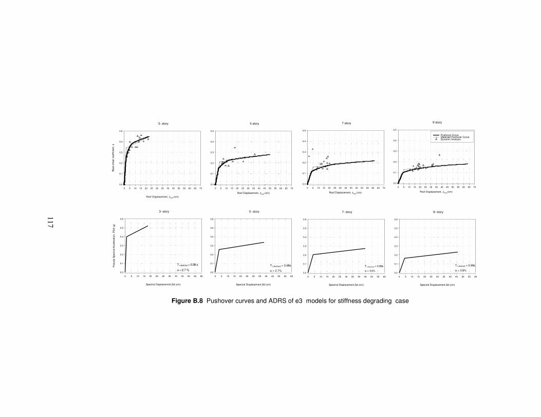
1
17
9 story
Roof Displacement, ∆roof (cm)
0 5 10 15 20 25 30 35 40 45 50 55 60 65 70
0.0
0.1
0.2
0.3
0.4
0.5
Pushover CurveIdealized Pushover CurveDynamic Analysis
3- story
Roof Displacement, ∆roof (cm)
0 5 10 15 20 25 30 35 40 45 50 55 60 65 70
Bas
e sh
ear
coef
ficie
nt,
η
0.0
0.1
0.2
0.3
0.4
0.5
5 story
Roof Displacement, ∆roof (cm)
0 5 10 15 20 25 30 35 40 45 50 55 60 65 70
0.0
0.1
0.2
0.3
0.4
0.5
7 story
Roof Displacement, ∆roof (cm)
0 5 10 15 20 25 30 35 40 45 50 55 60 65 70
0.0
0.1
0.2
0.3
0.4
0.5
3- story
Spectral Displacement,Sd (cm)
0 5 10 15 20 25 30 35 40 45 50 55 60
Pse
udo
Spe
ctra
l Acc
eler
atio
n, P
SA
(g)
0.0
0.1
0.2
0.3
0.4
0.5
0.6
T1,idealized = 0.38 s
α = 2.7 %
5- story
Spectral Displacement,Sd (cm)
0 5 10 15 20 25 30 35 40 45 50 55 60
0.0
0.1
0.2
0.3
0.4
0.5
0.6
T1,idealized = 0.68s
α = 2.7%
7- story
Spectral Displacement,Sd (cm)
0 5 10 15 20 25 30 35 40 45 50 55 60
0.0
0.1
0.2
0.3
0.4
0.5
0.6
T1,idealized = 0.89s
α = 3.5%
9- story
Spectral Displacement,Sd (cm)
0 5 10 15 20 25 30 35 40 45 50 55 60
0.0
0.1
0.2
0.3
0.4
0.5
0.6
T1,idealized = 0.99s
α = 3.9%
Figure B.8 Pushover curves and ADRS of e3 models for stiffness degrading case

1
18
9 story
Roof Displacement, ∆roof (cm)
0 5 10 15 20 25 30 35 40 45 50 55 60 65 70
0.00
0.05
0.10
0.15
0.20
0.25
0.30
0.35
Pushover CurveIdealized Pushover CurveDynamic Analysis
3- story
Roof Displacement, ∆roof (cm)
0 5 10 15 20 25 30 35 40 45 50
Bas
e sh
ear
coef
ficie
nt,
η
0.00
0.05
0.10
0.15
0.20
0.25
0.30
0.35
5 story
Roof Displacement, ∆roof (cm)
0 5 10 15 20 25 30 35 40 45 50 55 60 65 70
0.00
0.05
0.10
0.15
0.20
0.25
0.30
0.35
7 story
Roof Displacement, ∆roof (cm)
0 5 10 15 20 25 30 35 40 45 50 55 60 65 70
0.00
0.05
0.10
0.15
0.20
0.25
0.30
0.35
3- story
Spectral Displacement,Sd (cm)
0 5 10 15 20 25 30 35 40 45 50 55 60
Pse
udo
Sp
ectr
al A
ccel
era
tion,
PS
A (
g)
0.0
0.1
0.2
0.3
0.4
5- story
Spectral Displacement,Sd (cm)
0 5 10 15 20 25 30 35 40 45 50 55 60
0.0
0.1
0.2
0.3
0.4
7- story
Spectral Displacement,Sd (cm)
0 5 10 15 20 25 30 35 40 45 50 55 60
0.0
0.1
0.2
0.3
0.4
9- story
Spectral Displacement,Sd (cm)
0 5 10 15 20 25 30 35 40 45 50 55 60
0.0
0.1
0.2
0.3
0.4
T1,idealized = 0.67 s
α = 5.8%
T1,idealized = 1.03s
α = 4.3 %
T1,idealized = 1.13s
α = 4.2%
T1,idealized = 1.27 s
α = 5.1%
Figure B.9 Pushover curves and ADRS of e1’ models for stiffness degrading case
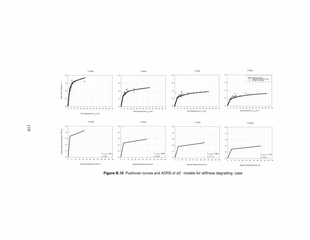
1
19
9 story
Roof Displacement, ∆roof (cm)
0 5 10 15 20 25 30 35 40 45 50 55 60 65 70
0.0
0.1
0.2
0.3
0.4
Pushover CurveIdealized Pushover CurveDynamic Analysis
3- story
Roof Displacement, ∆roof (cm)
0 5 10 15 20 25 30 35 40 45 50 55 60 65 70
Bas
e sh
ear
coef
ficie
nt,
η
0.0
0.1
0.2
0.3
0.4
5 story
Roof Displacement, ∆roof (cm)
0 5 10 15 20 25 30 35 40 45 50 55 60 65 70
0.0
0.1
0.2
0.3
0.4
7 story
Roof Displacement, ∆roof (cm)
0 5 10 15 20 25 30 35 40 45 50 55 60 65 70
0.0
0.1
0.2
0.3
0.4
3- story
Spectral Displacement,Sd (cm)
0 5 10 15 20 25 30 35 40 45 50 55 60
Pse
udo
Spe
ctra
l Acc
eler
atio
n, P
SA
(g)
0.0
0.1
0.2
0.3
0.4
0.5
5- story
Spectral Displacement,Sd (cm)
0 5 10 15 20 25 30 35 40 45 50 55 60
0.0
0.1
0.2
0.3
0.4
0.5
7- story
Spectral Displacement,Sd (cm)
0 5 10 15 20 25 30 35 40 45 50 55 60
0.0
0.1
0.2
0.3
0.4
0.5
T1,idealized = 0.99 s
α = 4.1 %
9- story
Spectral Displacement,Sd (cm)
0 5 10 15 20 25 30 35 40 45 50 55 60
0.0
0.1
0.2
0.3
0.4
0.5
T1,idealized = 0.56 s
α = 3.8%
T1,idealized = 0.82s
α = 3.5%
T1,idealized = 1.13s
α = 4.2 %
Figure B.10 Pushover curves and ADRS of e2’ models for stiffness degrading case

1
20
9 story
Roof Displacement, ∆roof (cm)
0 5 10 15 20 25 30
0.00
0.02
0.04
0.06
0.08
0.10
0.12
0.14
0.16
0.18
Pushover CurveIdealized Pushover CurveDynamic Analysis
3- story
Roof Displacement, ∆roof (cm)
0 5 10 15 20 25 30
Ba
se s
hea
r co
effic
ient
, η
0.00
0.02
0.04
0.06
0.08
0.10
0.12
0.14
0.16
0.18
5 story
Roof Displacement, ∆roof (cm)
0 5 10 15 20 25 30
0.00
0.02
0.04
0.06
0.08
0.10
0.12
0.14
0.16
0.18
7 story
Roof Displacement, ∆roof (cm)
0 5 10 15 20 25 30
0.00
0.02
0.04
0.06
0.08
0.10
0.12
0.14
0.16
0.18
3- story
Spectral Displacement,Sd (cm)
0 5 10 15 20 25
Pse
udo
Spe
ctra
l Acc
eler
atio
n, P
SA
(g)
0.00
0.02
0.04
0.06
0.08
0.10
0.12
0.14
0.16
0.18
0.20
T1,idealized = 0.76 s
α = 15.5%
5- story
Spectral Displacement,Sd (cm)
0 5 10 15 20 25
0.00
0.02
0.04
0.06
0.08
0.10
0.12
0.14
0.16
0.18
0.20
T1,idealized = 1.04 s
α = 14%
7- story
Spectral Displacement,Sd (cm)
0 5 10 15 20 25
0.00
0.02
0.04
0.06
0.08
0.10
0.12
0.14
0.16
0.18
0.20
T1,idealized = 1.44 s
α = 2.8 %
9- story
Spectral Displacement,Sd (cm)
0 5 10 15 20 25
0.00
0.02
0.04
0.06
0.08
0.10
0.12
0.14
0.16
0.18
0.20
T1,idealized = 1.28 s
α = 2.5 %
Figure B.11 Pushover curves and ADRS of e1 models for stiffness and strength degrading case

1
21
9 story
Roof Displacement, ∆roof (cm)
0 5 10 15 20 25 30 35 40
0.00
0.05
0.10
0.15
0.20
0.25
0.30
0.35
Pushover CurveIdealized Pushover CurveDynamic Analysis
3- story
Roof Displacement, ∆roof (cm)
0 5 10 15 20 25 30 35 40 45 50
Ba
se s
hea
r co
effic
ient
, η
0.00
0.05
0.10
0.15
0.20
0.25
0.30
5 story
Roof Displacement, ∆roof (cm)
0 5 10 15 20 25 30 35 40 45 50
0.0
0.1
0.2
0.3
7 story
Roof Displacement, ∆roof (cm)
0 5 10 15 20 25 30 35 40 45 50
0.00
0.05
0.10
0.15
0.20
0.25
0.30
0.35
3- story
Spectral Displacement,Sd (cm)
0 5 10 15 20 25 30 35 40
Pse
udo
Spe
ctra
l Acc
eler
atio
n, P
SA
(g)
0.00
0.05
0.10
0.15
0.20
0.25
0.30
T1,idealized = 0.62 s
α = 7.6 %
5- story
Spectral Displacement,Sd (cm)
0 5 10 15 20 25 30 35 40
0.00
0.05
0.10
0.15
0.20
0.25
0.30
0.35
T1,idealized = 0.82s
α = 4.2%
7- story
Spectral Displacement,Sd (cm)
0 5 10 15 20 25 30 35 40
0.00
0.05
0.10
0.15
0.20
0.25
0.30
0.35
T1,idealized = 0.99s
α = 1.8 %
9- story
Spectral Displacement,Sd (cm)
0 5 10 15 20 25 30 35 40
0.00
0.05
0.10
0.15
0.20
0.25
0.30
0.35
T1,idealized = 1.13 s
α = 2.4 %
Figure B.12 Pushover curves and ADRS of e2 models for stiffness and strength degrading case

1
22
9 story
Roof Displacement, ∆roof (cm)
0 5 10 15 20 25 30 35 40 45
0.0
0.1
0.2
0.3
0.4
0.5
Pushover CurveIdealized Pushover CurveDynamic Analysis
3- story
Roof Displacement, ∆roof (cm)
0 5 10 15 20 25 30 35 40 45 50 55 60 65 70
Bas
e sh
ear
coef
ficie
nt,
η
0.0
0.1
0.2
0.3
0.4
0.5
5 story
Roof Displacement, ∆roof (cm)
0 5 10 15 20 25 30 35 40 45 50 55 60 65 70
0.0
0.1
0.2
0.3
0.4
0.5
7 story
Roof Displacement, ∆roof (cm)
0 5 10 15 20 25 30 35 40 45 50 55 60 65 70
0.0
0.1
0.2
0.3
0.4
0.5
3- story
Spectral Displacement,Sd (cm)
0 5 10 15 20 25 30 35 40 45 50 55 60
Pse
udo
Spe
ctra
l Acc
eler
atio
n, P
SA
(g)
0.0
0.1
0.2
0.3
0.4
0.5
0.6
T1,idealized = 0.38 s
α = 2.6 %
5- story
Spectral Displacement,Sd (cm)
0 5 10 15 20 25 30 35 40 45 50 55 60
0.0
0.1
0.2
0.3
0.4
0.5
0.6
T1,idealized = 0.68 s
α = 3.8 %
7- story
Spectral Displacement,Sd (cm)
0 5 10 15 20 25 30 35 40 45
0.0
0.1
0.2
0.3
0.4
0.5
0.6
T1,idealized = 0.89 s
α = 2.2%
9- story
Spectral Displacement,Sd (cm)
0 5 10 15 20 25 30 35 40 45
0.0
0.1
0.2
0.3
0.4
0.5
0.6
T1,idealized = 0.99 s
α = 2.4%
Figure B.13 Pushover curves and ADRS of e3 models for stiffness and strength degrading case

1
23
9 story
Roof Displacement, ∆roof (cm)
0 5 10 15 20 25 30 35 40 45 50 55 60 65 70
0.00
0.05
0.10
0.15
0.20
0.25
0.30
Pushover CurveIdealized Pushover CurveDynamic Analysis
3- story
Roof Displacement, ∆roof (cm)
0 5 10 15 20 25 30 35 40 45 50
Bas
e sh
ear
coef
ficie
nt, η
0.00
0.05
0.10
0.15
0.20
0.25
0.30
5 story
Roof Displacement, ∆roof (cm)
0 5 10 15 20 25 30 35 40 45 50 55 60 65 70
0.00
0.05
0.10
0.15
0.20
0.25
0.30
7 story
Roof Displacement, ∆roof (cm)
0 5 10 15 20 25 30 35 40 45 50 55 60 65 70
0.00
0.05
0.10
0.15
0.20
0.25
0.30
3- story
Spectral Displacement,Sd (cm)
0 5 10 15 20 25 30 35 40 45 50 55 60
Pse
udo
Spe
ctra
l Acc
eler
atio
n, P
SA
(g)
0.00
0.05
0.10
0.15
0.20
0.25
0.30
0.35
T1,idealized = 0.67 s
α = 5.3 %
5- story
Spectral Displacement,Sd (cm)
0 5 10 15 20 25 30 35 40 45 50 55 60
0.0
0.1
0.2
0.3
T1,idealized = 1.03 s
α = 3.9 %
7- story
Spectral Displacement,Sd (cm)
0 5 10 15 20 25 30 35 40 45 50 55 60
0.00
0.05
0.10
0.15
0.20
0.25
0.30
0.35
T1,idealized = 1.13 s
α = 2.2 %
9- story
Spectral Displacement,Sd (cm)
0 5 10 15 20 25 30 35 40 45 50 55 60
0.00
0.05
0.10
0.15
0.20
0.25
0.30
0.35
T1,idealized = 1.27 s
α = 1 %
Figure B.14 Pushover curves and ADRS of e1’ models for stiffness and strength degrading case

1
24
9 story
Roof Displacement, ∆roof (cm)
0 5 10 15 20 25 30 35 40 45 50
0.00
0.05
0.10
0.15
0.20
0.25
0.30
0.35
Pushover CurveIdealized Pushover CurveDynamic Analysis
3- story
Roof Displacement, ∆roof (cm)
0 5 10 15 20 25 30 35 40 45 50
Ba
se s
hea
r co
effic
ient
, η
0.00
0.05
0.10
0.15
0.20
0.25
0.30
0.35
5 story
Roof Displacement, ∆roof (cm)
0 5 10 15 20 25 30 35 40 45 50
0.00
0.05
0.10
0.15
0.20
0.25
0.30
0.35
7 story
Roof Displacement, ∆roof (cm)
0 5 10 15 20 25 30 35 40 45 50
0.00
0.05
0.10
0.15
0.20
0.25
0.30
0.35
3- story
Spectral Displacement,Sd (cm)
0 5 10 15 20 25 30 35 40
Pse
udo
Spe
ctra
l Acc
eler
atio
n, P
SA
(g)
0.00
0.05
0.10
0.15
0.20
0.25
0.30
0.35
T1,idealized = 0.56 s
α = 5.3 %
5- story
Spectral Displacement,Sd (cm)
0 5 10 15 20 25 30 35 40
0.00
0.05
0.10
0.15
0.20
0.25
0.30
0.35
T1,idealized = 0.82 s
α = 2.1%
7- story
Spectral Displacement,Sd (cm)
0 5 10 15 20 25 30 35 40
0.00
0.05
0.10
0.15
0.20
0.25
0.30
0.35
T1,idealized = 0.99s
α = 2.2 %
9- story
Spectral Displacement,Sd (cm)
0 5 10 15 20 25 30 35 40
0.00
0.05
0.10
0.15
0.20
0.25
0.30
0.35
T1,idealized = 1.13s
α = 1.8 %
Figure B.15 Pushover curves and ADRS of e2’ models for stiffness and strength degrading case
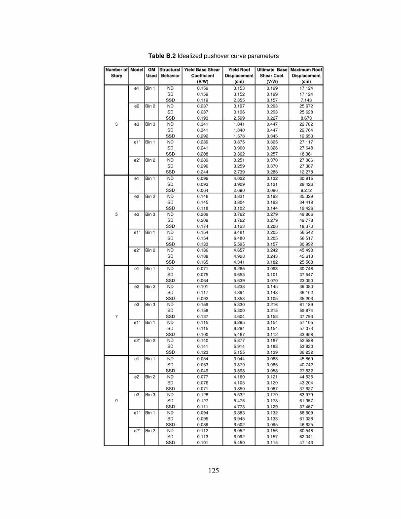
125
Table B.2 Idealized pushover curve parameters
Number of Model GM Structural Yield Base Shear Yield Roof Ultimate Base Maximum RoofStory Used Behavior Coefficient Displacement Shear Coef. Displacement
(V/W) (cm) (V/W) (cm)
e1 Bin 1 ND 0.159 3.153 0.199 17.124SD 0.159 3.152 0.199 17.124
SSD 0.119 2.355 0.157 7.143e2 Bin 2 ND 0.237 3.197 0.293 25.672
SD 0.237 3.196 0.293 25.628SSD 0.193 2.599 0.227 8.673
3 e3 Bin 3 ND 0.341 1.841 0.447 22.782SD 0.341 1.840 0.447 22.764
SSD 0.292 1.578 0.345 12.653e1' Bin 1 ND 0.239 3.875 0.325 27.117
SD 0.241 3.900 0.326 27.648SSD 0.208 3.362 0.257 18.361
e2' Bin 2 ND 0.289 3.251 0.370 27.086SD 0.290 3.259 0.370 27.387
SSD 0.244 2.739 0.288 12.278
e1 Bin 1 ND 0.096 4.022 0.132 30.915SD 0.093 3.909 0.131 28.426
SSD 0.064 2.690 0.086 9.272e2 Bin 2 ND 0.146 3.831 0.193 35.329
SD 0.145 3.804 0.193 34.418SSD 0.118 3.102 0.144 19.426
5 e3 Bin 3 ND 0.209 3.762 0.279 49.806SD 0.209 3.762 0.279 49.778
SSD 0.174 3.123 0.206 18.370e1' Bin 1 ND 0.154 6.481 0.205 56.542
SD 0.154 6.480 0.205 56.517SSD 0.133 5.595 0.157 30.992
e2' Bin 2 ND 0.186 4.657 0.242 45.493SD 0.188 4.928 0.243 45.613
SSD 0.165 4.341 0.182 25.568
e1 Bin 1 ND 0.071 6.265 0.098 30.748SD 0.075 6.653 0.101 37.547
SSD 0.064 5.639 0.070 23.350e2 Bin 2 ND 0.101 4.238 0.145 39.080
SD 0.117 4.894 0.143 36.102SSD 0.092 3.853 0.105 35.203
e3 Bin 3 ND 0.159 5.330 0.216 61.189SD 0.158 5.300 0.215 59.874
7 SSD 0.137 4.604 0.158 37.793e1' Bin 1 ND 0.115 6.295 0.154 57.105
SD 0.115 6.294 0.154 57.073SSD 0.100 5.467 0.112 33.958
e2' Bin 2 ND 0.140 5.877 0.187 52.588SD 0.141 5.914 0.188 53.820
SSD 0.123 5.155 0.139 36.232
e1 Bin 1 ND 0.054 3.944 0.088 45.869SD 0.053 3.879 0.085 40.742
SSD 0.049 3.598 0.058 27.532e2 Bin 2 ND 0.077 4.160 0.121 44.535
SD 0.076 4.105 0.120 43.204SSD 0.071 3.850 0.087 37.627
e3 Bin 3 ND 0.128 5.532 0.179 63.9799 SD 0.127 5.475 0.178 61.957
SSD 0.111 4.773 0.129 37.467e1' Bin 1 ND 0.094 6.883 0.132 58.509
SD 0.095 6.945 0.133 61.028SSD 0.089 6.502 0.095 46.625
e2' Bin 2 ND 0.112 6.052 0.156 60.548SD 0.113 6.092 0.157 62.041
SSD 0.101 5.450 0.115 47.143

126
APPENDIX C
PREDICTION EQUATIONS FOR GROUND MOTION AND ELASTIC
SPECTRAL DISPLACEMENT
C.1 Prediction Equation for ground motion (Akkar and Bommer,
2007)
The prediction equation is derived by using the strong-motion database
for seismically active areas of Europe and the Middle East only for
PGV. The explanatory variables in the equation are magnitude, Joyner-
Boore distance, site class and style-of-faulting. The functional form is
provided in equation C.1.
NNA
sjbxx
FbFbSb
SbbRMbbMbMbbPGV
1098
7
2
6
2
54
2
321 )log()()log(
+++
++++++= (C.1)
where M is magnitude; SA and SS are dummy variables representing the
influence of site class, taking values of 1 for stiff and soft soil sites,
respectively, and zero otherwise; FN and FR are dummy values of 1 for
normal and reverse ruptures respectively, and zero otherwise. Subscript
xx denotes either GM or max. Regression coefficients from b1-b10 are
given in Table C.1.
Table C.1 Regression coefficients of the prediction equation
Eq. b1 b2 b3 b4 b5 b6 b7 b8 b9 b10
GM -1.36 1.063 -0.079 -2.948 0.306 5.547 0.243 0.087 -0.057 0.0245
MAX -1.26 1.103 -0.085 -3.103 0.327 5.504 0.226 0.079 -0.083 0.0116
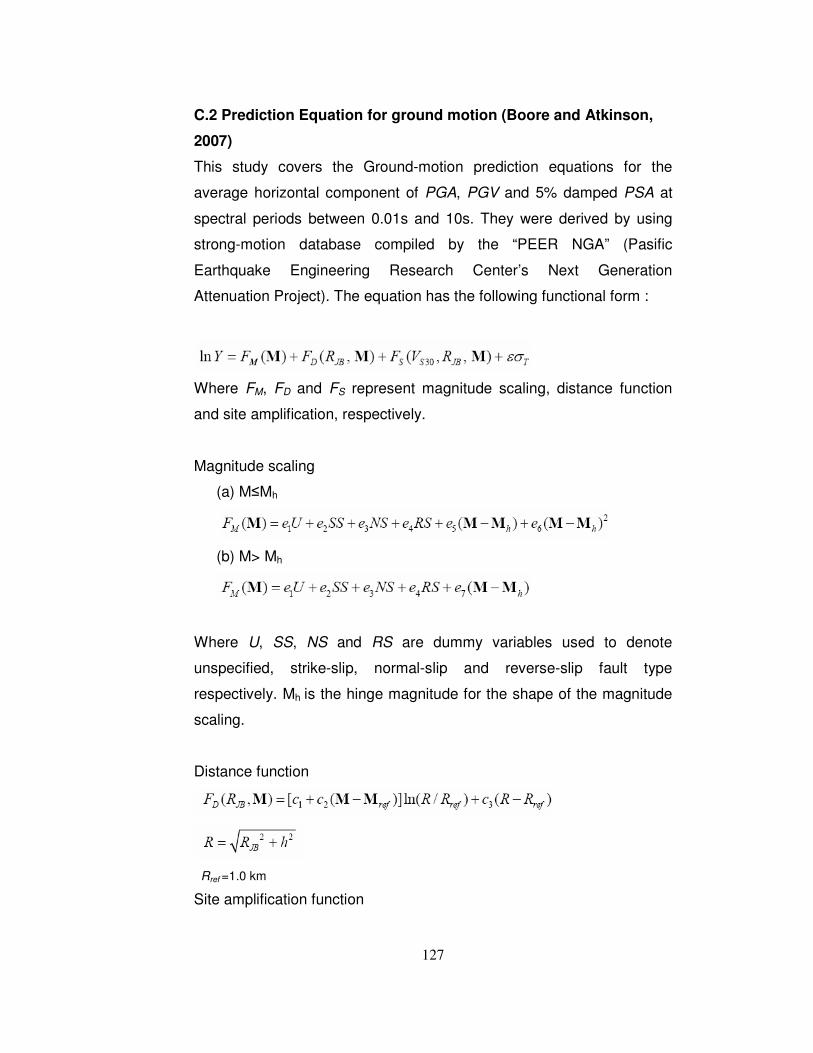
127
C.2 Prediction Equation for ground motion (Boore and Atkinson,
2007)
This study covers the Ground-motion prediction equations for the
average horizontal component of PGA, PGV and 5% damped PSA at
spectral periods between 0.01s and 10s. They were derived by using
strong-motion database compiled by the “PEER NGA” (Pasific
Earthquake Engineering Research Center’s Next Generation
Attenuation Project). The equation has the following functional form :
Where FM, FD and FS represent magnitude scaling, distance function
and site amplification, respectively.
Magnitude scaling
(a) M≤Mh
(b) M> Mh
Where U, SS, NS and RS are dummy variables used to denote
unspecified, strike-slip, normal-slip and reverse-slip fault type
respectively. Mh is the hinge magnitude for the shape of the magnitude
scaling.
Distance function
Rref =1.0 km
Site amplification function

128
Linear term
Nonlinear term
The details of the prediction equations can be seen in the related article
Boore and Atkinson (2007).

129
C.3 Prediction Equation for spectral displacement (Akkar and
Bommer, 2007b)
This empirical equation for the prediction of displacement response
ordinates is derived using the strong motion databank from Europe and
the Middle East. The functional form selected for the the equation is the
same as that used by Akkar and Bommer (2007a) for the prediction of
PGV.
[ ]
RNA
Sjb
FbFbSb
SbbRMbbMbMbbTSD
1098
7
2
6
2
54
2
321 log)(),(log
+++
++++++=ξ
Where M is moment magnitude, Rjb is the Joyner-Boore distance in
kilometers, Ss and SA are binary variables taking values 1 for soft and
stiff soil sites, respectively (and zero otherwise) and FN and FR are
similarly derived for normal and reverse faulting earthquakes.
Regression coefficients are provided for different period and damping
values in the related article.