Embed Size (px)
Citation preview

Directed Assistance Module 6 (DAM6):
Filter Assessments: Understanding What You See
Prepared by:
Texas Commission on Environmental Quality
Water Supply Division
Texas Optimization Program (TOP)
Latest revision date: 8/24/19

i
i
Table of Contents Table of Figures ................................................................................ iv
Section 1: Introduction to Filter Assessments ................................. 1
1.1 Assumptions ....................................................................................... 1 1.2 Why Improve on “Acceptable” Filter Performance ............................. 1
1.2.1 Reduced Cost of Operation ................................................................ 1 1.2.2 Reduced Public Health Risk ................................................................ 1 1.2.3 Improved Filter Value ....................................................................... 4
1.3 Approach ............................................................................................ 4 1.4 Practical Applications ......................................................................... 5 1.5 Assessment of Routinely Collected Data ............................................. 5 1.6 Routine Observations and Maintenance.............................................. 6 1.7 Special Studies ................................................................................... 6 1.8 Other Resources ................................................................................. 7
Section 2: Routine Data Analyses ..................................................... 8
2.1 Data Collection ................................................................................... 8 2.1.1 Operator Logs (Bench Sheets) ........................................................... 8 2.1.2 Strip/Circular Charts ......................................................................... 9 2.1.3 SCADA Records ................................................................................ 9 2.1.4 Surface Water Monthly Operating Reports (SWMORs) ......................... 10
2.2 Data Assembly ................................................................................. 10 2.2.1 Baseline Filter Performance ............................................................. 10 2.2.2 Manual Data Assembly .................................................................... 11 2.2.3 Strip/Circular Chart Data ................................................................. 12 2.2.4 Electronic Records .......................................................................... 12 2.2.5 Comparison of Filter Performance to Other Data................................. 14 2.2.6 Exclusion of Some Data .................................................................. 14
2.3 Data Analyses................................................................................... 15 2.3.1 IFE Turbidity Profiles ...................................................................... 15 2.3.2 Analyzing Head Loss Trends ............................................................ 32 2.3.3 Analyzing Filter Productivity Trends .................................................. 39
2.4 Data Analysis Summary .................................................................... 43
Section 3: Routine Observations and Maintenance ......................... 44
3.1 Routine Visual Observations ............................................................. 44
ii
3.1.1 Air Releases .................................................................................. 44 3.1.2 Changes in Media Depth .................................................................. 45 3.1.3 Mudballs ....................................................................................... 46 3.1.4 Filter Backwash Irregularities ........................................................... 48 3.1.5 Media Surface Irregularities ............................................................. 57 3.1.6 Filter Box Cross Connections ............................................................ 64
3.2 Plant Noise ....................................................................................... 66 3.2.1 Motor Driven Valves ....................................................................... 66 3.2.2 Pipe Noise ..................................................................................... 66
3.3 Routine Equipment Maintenance ...................................................... 67 3.3.1 Monitors and Recorders................................................................... 67 3.3.2 Other Filter Monitors and Controllers ................................................ 71
Section 4: Special Studies for Filters ............................................. 72
4.1 Introduction ..................................................................................... 72 4.2 Flow Metering and Flow Control Calculations ................................... 72
4.2.1 Hook Gauges ................................................................................. 72 4.2.3 Effluent Flow Meters and Flow Controllers .......................................... 75 4.2.4 Backwash Flow Meters and Controllers .............................................. 75
4.3 Filter Influent Flow Controllers ........................................................ 75 4.3.1 Understanding Water Momentum ..................................................... 76 4.3.2 Pipe Weirs ..................................................................................... 79
4.4 Filter Probes and Excavation ............................................................ 82 4.4.1 Safety ........................................................................................... 82 4.4.2 Filter Probing ................................................................................. 83 4.4.4 Media Excavations .......................................................................... 87
4.5 Backwash Rise Rate and Bed Expansion ........................................... 92 4.5.1 Rise Rate ...................................................................................... 92 4.5.2 Bed Expansion ............................................................................... 94
4.5 Media Condition ................................................................................ 97 4.5.1 Sieve Analysis................................................................................ 97 4.5.2 Media Density .............................................................................. 104 4.5.3 Microscopic Inspection .................................................................. 105 4.5.4 Solubility Tests ............................................................................ 107 4.5.5 Mudball Content ........................................................................... 114 4.5.6 Floc Retention Analysis ................................................................. 116
Appendix A: Student Guide ............................................................... 1
Workshop 1: Why Optimize? .................................................................... 1
iii
Workshop 2: Introduction to Trend Analysis ........................................... 3 Workshop 3: Compiling and Using Routinely Collected Data .................. 11 Workshop 4: Conducting a Filter Inspection ........................................... 13
Equation 1: Calculating filtration rate: ....................................................... 19 Equation 2: Calculating the backwash water flow rate ................................ 28 Equation 3: Calculating the Percent bed expansion .................................... 28
Appendix B: Filter Maintenance Guidelines ....................................... 1
Filter Bed Inspection ................................................................................ 1 Filter Media Cleanliness ............................................................................ 4 Skimming ................................................................................................. 5 Filter Bed Expansion ................................................................................. 7 Backwash Rise Rate Adjustments .......................................................... 10 Placing a Filter ln/Out of Service ........................................................... 11 Filter Bed Media Stock Measuring ........................................................... 12 Filter Turbidity and Headloss Analyses ................................................... 15 Guidelines for Working in a Filter ........................................................... 19 Filter Bed Historical Records .................................................................. 20 Communication ...................................................................................... 21
Appendix C: Filter Coring Procedures .............................................. 1
Appendix D: References .................................................................... 1
Appendix E: Definitions and Acronyms ............................................ 1
DAM 6. Evaluation Form ................................................................... 7

iv
Table of Figures Figure 1: Impact of Post-Backwash Recovery Spikes on Cumulative Particle
Removal of a Filter .......................................................................... 3 Figure 2: Impact of Valve Operation on the Post-Backwash Recovery Spike ........... 4 Figure 3: Filter Production Table .................................................................... 11 Figure 4: Data Table Assembled From SCADA IFE Turbidity Records ................... 13 Figure 5: Annual IFE Turbidity Profile (Max. Daily) ........................................... 15 Figure 6: Comparison of Maximum Daily IFE Turbidities for Multiple Filters .......... 16 Figure 7: Frequency Plot of Max Daily IFE Turbidities ........................................ 17 Figure 8: Chart Comparing IFE Turbidity Records to other Parameters ................ 18 Figure 9: Comparing Filter Performance .......................................................... 19 Figure 10: 24-hour IFE Turbidity Profile - 15-Minute Data ................................. 20 Figure 11: 24-hour IFE Turbidity Profile Comparing 15-Minute Data with One-
Minute Data .................................................................................. 21 Figure 12: Plant Flow Diagram ....................................................................... 22 Figure 13: IFE Turbidity Profile Resulting from Severe Hydraulic Fluctuations ...... 23 Figure 14: Atypical (Unusual) IFE Turbidity Profile: Flow Diagram ...................... 24 Figure 15: Atypical (Non-typical) IFE Turbidity Profile: Turbidity Profile ............... 25 Figure 16: Idealized IFE Turbidity Profile for a Filter Run ................................... 26 Figure 17: Idealized Backwash Cycle .............................................................. 28 Figure 18: Atypical (Non-typical) Filter Backwash Spike .................................... 29 Figure 19: Percentage of Turbidity Removed Chart ........................................... 31 Figure 20: Carman-Kozeny Equation .............................................................. 32 Figure 21: The Factors in the Carman-Kozeny Equation .................................... 33 Figure 22: Simplified Representation of the Carman-Kozeny Equation ................ 36 Figure 23: Flow Through Clean vs. Dirty Media ................................................ 37 Figure 24: Filter Head Loss vs. Filter Run-Time ................................................ 38 Figure 25: Pressure at Depth for Multiple Filter Run Volumes ............................. 38 Figure 26: Unit Filter Run Volume .................................................................. 40 Figure 27: Normalized Net Yield ..................................................................... 41 Figure 28: Filter Efficiency (Percent Net Yield) ................................................. 42 Figure 29: Filtered Water Transfer Tank with Sand and Anthracite ..................... 45 Figure 30: Mudball Effects ............................................................................. 47 Figure 31: Idealized Dispersion of Water During Backwash ................................ 49 Figure 32: Idealized Media Fluidization During Backwash .................................. 50 Figure 33: Irregular Air Scour and Backwash Water Distribution ........................ 53 Figure 34: Photograph of Severe Jetting ......................................................... 54
v
Figure 35: Sectional View of Severe Jetting ..................................................... 55 Figure 36: Examples of troughs that are not level ............................................ 56 Figure 37: Examples of Trough Flooding ......................................................... 57 Figure 38: Retraction Cracks ......................................................................... 58 Figure 39: Surface Accumulations: These really aren’t cracks… It’s dried floc on top
of a filter that was drained before backwashing. ................................ 59 Figure 40: Mounds and Depressions (1) .......................................................... 60 Figure 41: Mounds and Depressions (2) .......................................................... 61 Figure 42: Post-Backwash Media Loss ............................................................. 63 Figure 43: Illustration of a Filter Box Cross Connection ..................................... 64 Figure 44: Filter Box Cross Connection ........................................................... 65 Figure 45: Manipulation of Instrument Output ................................................. 68 Figure 46: Instrument Performance Before and After Cleaning ........................... 69 Figure 47: Circular Chart Record of IFE Turbidity ............................................. 70 Figure 48: Typical Hook Gauge ...................................................................... 72 Figure 49: Using a Hook Gauge ..................................................................... 73 Figure 50: Calculating Flow Rate .................................................................... 74 Figure 51: Flow Splitting with a Splitter Box .................................................... 77 Figure 52: Effects of Velocity Head in a Splitter Box ......................................... 78 Figure 53: Splitter Box with Pipe Weirs ........................................................... 79 Figure 54: Cross-Section of a Poorly Designed Splitter Box................................ 80 Figure 55: Splitter Box with Pipe Weirs ........................................................... 81 Figure 56: Safety Gear for Working In Filters ................................................... 82 Figure 57: TCEQ Investigator Using a Filter Probe ............................................ 83 Figure 58: Filter Probe Plan for a Small, 1-Trough Filter .................................... 84 Figure 59: Collecting Filter Probe Data ............................................................ 85 Figure 60: Bed Uniformity and Thickness ........................................................ 86 Figure 61: Checking for Media Stratification and Mudballs ................................. 88 Figure 62: Mud in the Media Bed .................................................................... 89 Figure 63: Photo of Poor Media Stratification ................................................... 90 Figure 64: Poor Media Stratification ................................................................ 91 Figure 65: Calculating Rise Rate .................................................................... 93 Figure 66: Calculating Bed Expansion ............................................................. 94 Figure 67: Bed Expansion Measurement Tools ................................................. 95 Figure 68: Two Engineers Measure Bed Expansion ........................................... 96 Figure 69: Sieve Analysis Equipment Set (1) ................................................... 98 Figure 70: Sieve Analysis Equipment (2) ......................................................... 99 Figure 71: Sieve Table: Effective Size and Uniformity Coefficient Calculator ..... 100
vi
Figure 72: Media Size Distribution Chart ....................................................... 101 Figure 73: Uniformity Coefficient Table ......................................................... 102 Figure 74: L/d Ratio Calculations.................................................................. 103 Figure 75: Density Calculations .................................................................... 104 Figure 76: Microscopic Examination of Good and Poor Media ........................... 106 Figure 77: Solvent Appearance During Media Grain Acidification ...................... 108 Figure 78: Appearance of Media Before and After Acidification ......................... 108 Figure 79: Media Grain Volume and Appearance Before and After Acid/Base
Cleaning ..................................................................................... 109 Figure 80: Calculating Percent Solubility ....................................................... 110 Figure 81: Comparison of Media Specifications – Before and After Acidification . 111 Figure 82: L/d Ratio Calculation for a Media Bed ............................................ 112 Figure 83: L/d Ratio Calculation for an Old Media Bed ..................................... 113 Figure 84: Mudballs from a Poorly Maintained Filter ........................................ 115 Figure 85: Mudball Content Analysis ............................................................. 116 Figure 86: Floc Retention Analysis Guidelines ................................................ 117 Figure 87: Floc Retention Analysis Charts ...................................................... 118

DAM6: Filter Assessments SG Page 1 of 120
Filter Assessments
Understanding What You See
Section 1: Introduction to Filter Assessments
1.1 Assumptions This module is presented with the assumption that the operator will understand the information in terms of valid filter science related to the drinking water industry. The assumption is also made that the operator understands math terms; such as gpm/ft2 (gallons per minute per square foot), ft3 (cubic foot), etc.; and routine mathematical calculations related to surface water plant operation. Lastly, the assumption is made that the operator has at least a very basic ability to use computer spreadsheets to collect, organize, and chart filter performance data.
1.2 Why Improve on “Acceptable” Filter Performance If our filters are performing within the limits of regulatory requirements, why should we be concerned about assessing the performance of the filters?
1.2.1 Reduced Cost of Operation
When filters are performing optimally, costs of operation can go down. Savings may accrue from:
• longer filter runs,
• reduced filter backwash volumes,
• longer useful life of the filter media, and/or
• lower filter maintenance costs.
1.2.2 Reduced Public Health Risk
Why have filters at all? Filters are the last barrier in the surface water treatment plant where pathogens are physically removed from the water, and the primary function of filters is to make water safer for human consumption. There are other reasons for making water cleaner, but the most important reason for the drinking water regulations is that human health is at risk when pathogens in the source water are not removed. Very generally, particle (turbidity) removal is correlated to pathogen removal, and many scientific studies confirm this. Though it is impractical to define an exact relationship between numbers of pathogens and
DAM6: Filter Assessments SG Page 2 of 120
numbers of particles in water, it follows that preventing particle breakthrough in a filter will prevent breakthrough of pathogens.
1.2.2.1 Particle Removal at Different Phases of Operation
The University of Waterloo (Emelko, 2000) performed a pilot scale study to assess Cryptosporidium removal with filtration during three phases of filter operation: (1) an extended period of relatively stable post-ripening1 operation; (2) a short period of slowly decreasing filter performance near the end of the filter cycle; and (3) at the point where the filtered water turbidity is no longer acceptable and the filter must be backwashed in order to meet filtered water quality goals. Their findings were:
• During the more stable parts of the filter cycle, their filter achieved up to 5 or 6-log (99.999 to 99.9999 percent) pathogen removal and the effluent turbidity was approximately 0.04 Nephelometric turbidity units (NTU).
• Near the end of the parts of the filter cycle, their filter achieved only 2 to 3-log (99 to 99.9 percent) pathogen removal and the effluent turbidity was approximately 0.10 NTU.
• At the filter breakthrough part of the cycle, their filter achieved only 1.5 to 2-log (97 to 99 percent) pathogen removal and the effluent turbidity was approximately 0.3 NTU.
A similar study pertaining to particle removal, as opposed to pathogen removal, (Amirtharajah, 1998) showed that 90% of the particles passing through a well-operated filter do so during filter ripening. Emelko’s and Amirtharajah’s findings show that as effluent turbidity increases, the number of pathogens passing through a filter increases exponentially.
1.2.2.2 Reduced Particle Removal during Filter Ripening
During filter ripening, the total number of pathogens which may pass through a filter is very high. If, for example, 90 percent of the particles passing through a filter pass during the filter ripening period following a backwash, then minimizing the duration of the ripening period and reducing the magnitude of the post-
1 “Ripening” is discussed later in this guide. Very generally, the application of settled water to the freshly washed filter bed, conditions the surfaces of the individual filter media grains (or ripens them) so that they attach to and hold particles more efficiently. Other elements of the filter cycle are discussed in detail in Subsection 2.3.1.4.

DAM6: Filter Assessments SG Page 3 of 120
backwash turbidity/particle spike would reduce the number of pathogens passing through a filter.
Figure 1 shows the performance of a filter during the filter ripening (post-backwash) period in terms of particle count and turbidity. The figure shows that as time passes, the filter allows fewer and fewer particles to pass, and the peak number of particles per ml at twenty-four minutes following the backwash is almost 100 times more than the count at 75 minutes following backwash. Amirtharajah’s conclusion that 90% of the particles passing through a filter will do so during the filter ripening period is not at all farfetched.
Figure 1: Impact of Post-Backwash Recovery Spikes on Cumulative Particle Removal of a Filter
1.2.2.3 Reducing the Impact of Periods of Poor Particle Removal
Post-backwash turbidity spikes are something that every system has to deal with. Figure 2 shows an example of the number of particles passing through a filter.

DAM6: Filter Assessments SG Page 4 of 120
Figure 2: Impact of Valve Operation on the Post-Backwash Recovery Spike
When the post-backwash flow through the filter was controlled by a fluctuating, poorly-controlled valve, the number of particles passing through the filter was high. When the poorly operating valve was replaced by a smoothly-opening valve, the spike is reduced. The total number of particles passing with the fluctuating valve was almost five times the number passing through the filter after the smoothly-opening valve had been installed. The recovery time for the filter with the smoothly-opening valve was also greatly reduced.
1.2.3 Improved Filter Value
In the example above, a single control factor (installing a better valve) was used to reduce the number of particles passing through the filter to 21% of the previous number. The “value” of the filter, in terms of particle removal, was improved almost five times. This manual was written to help operators to cost-effectively increase the value of the filters they operate.
1.3 Approach Each part of a surface water treatment plant (SWTP), and each component in water treatment can be, and most often is, intricately related to other components. However, the focus of this module will be on the filter and the most directly

DAM6: Filter Assessments SG Page 5 of 120
associated appurtenances. This is not to disregard the importance or impact of the other treatment units on the filters and finished water quality: it is only to limit the scope of this module/manual to the essential principles of filter assessment.
Most of the information in this module/manual is based on field studies by the TCEQ’s staff in the Field Offices and the Water Supply Division. Almost all photos, graphs, tables, and examples in this document come from staff assessments at surface water treatment plants in Texas. Published references are also provided for additional clarification.
The module contains practical exercises, including assembly of some performance data for interpretation, and a filter assessment which includes several special studies. Appendix A has a “Student Guide” to facilitate execution of these exercises.
1.4 Practical Applications All operators perform filter assessments, though they do not often think of them in these terms. An assessment may be as simple as a glance at the individual effluent (IFE) turbidity reading, the head-loss gauge, or the filter run-time and making a mental note that something must be done in the near future. Under normal operating conditions, such observations can be used to reliably predict the filter’s potential for continuing acceptable performance or incipient degrading performance, and allow the operator to respond accordingly. This type of simple filter assessment, or even the most intensive filter assessment, usually verifies that the filter and the peripheral equipment are working fine. Sometimes, however, they help the operator figure out when the filter is not performing as it should, and sometimes indicates the cause of the substandard performance. This manual also provides a systematic approach for collecting and assembling filter performance data and a framework for interpreting this data.
1.5 Assessment of Routinely Collected Data Routine data analyses include:
• IFE turbidity profiles
• Head loss trends
• Filter productivity trends
• Unit comparisons
Although some operators routinely examine the current status of their filter in terms of effluent turbidity, head loss, and production, other operators may fail to evaluate and fail to see the importance of comparing the performance profiles or

DAM6: Filter Assessments SG Page 6 of 120
head loss trends of an individual filter over a period of days, weeks or months. Typically, operators have a current working knowledge of how the filter has performed since the last backwash and what the current value of each performance parameter means in terms of a particular filter run. But every major element of the water production process is dynamic: the quality of raw water varies, pump performance degrades, sedimentation basin performance varies, valve performance degrades, and customer demands trend upward and downward. For these reasons, the routine data analyses should include evaluation of both long-term trends and short-term performance trends. These analyses will be discussed in detail in Section 2 of this manual.
1.6 Routine Observations and Maintenance Routine observations and maintenance, which will be discussed in detail in Section 3, are an integral part of filter assessment. Air releases during filter operation or backwash may indicate physical or plumbing problems. Changes in media surface conditions can indicate moderate to severe media degradation or loss. Backwash irregularities can point to structural or other engineering problems with a filter. Again, these points of information must be assembled in a useful framework and interpreted correctly to be of value to the operator.
1.7 Special Studies Special studies, which will be discussed in detail in Section 4, include topics such as:
• flow metering and control,
• filter probing and media excavations,
• rise rate and bed expansion,
• media size and condition,
• mudball content, and
• floc retention analysis.
When a filter is performing at a substandard level, special studies may be used to characterize the type and extent of a problem. However, it is best to use a subset of the special studies every 18 to 36-months to evaluate the filter’s condition, even if routine data analyses and routine observations do not indicate a problem.

DAM6: Filter Assessments SG Page 7 of 120
1.8 Other Resources This manual has several appendices to provide additional information to help the operator to enhance their knowledge and skills pertaining to filter assessments. These appendices include:
• Texas Regulatory Design and Operational Requirements;
• Sample Filter Maintenance Guidelines;
• Filter Coring Procedures;
• References; and
• Definitions, Acronyms, and Formulae.

DAM6: Filter Assessments SG Page 8 of 120
Section 2: Routine Data Analyses
2.1 Data Collection Routine data analyses involve utilization of data collected and recorded during normal operations, by the operator, strip/circular chart recorders, or the Supervisory Control and Data Acquisition (SCADA) system. This is fortunate, because effective data collection is the essential first step for filter data analysis. Even so, assembling turbidity data for investigative purposes may require collection of turbidity data at one-minute intervals rather than the normal 15-minute intervals for the duration of the assessment (and this might be a special study).
2.1.1 Operator Logs (Bench Sheets)
In this manual, the term “operator logs” is used to describe the bench sheets or other documents into which the operator manually enters information pertaining to routine analyses, chemical feed settings, flow rates, and other operations data. However, it does not have to be a single document. An “operator log” (singular) may be recorded on more than one form in more than one location in the plant. The operator logs are normally tailor-made by the plant staff to make collection of operations data manageable and to make the assembled data easy to interpret by the staff. Typically, they include tables in which to record data required to meet minimal reporting requirements, and most often, they also include areas for operations information that helps the operator understand the current status and performance of the plant. This discussion will focus on those data most commonly used in filter assessments.
As pertains to filter assessments, the operator logs will normally contain detailed information concerning the quality of the water entering the filters, the condition of water leaving the filters, and, other filter parameters. To facilitate use of the information, Operator logs must contain the dates and times the data were collected, and be accurate and precise enough to allow trending analysis. Further, the data must be clearly identified with the filter for which they were collected. The information most commonly recorded in Operator logs which are useful in filter assessments are:
• settled water quality data,
• Individual Filter Effluent (IFE) turbidity data,
• filter head loss data,
• filter production data, and
• calibration records for monitoring equipment.

DAM6: Filter Assessments SG Page 9 of 120
The data in the operator log must be collected and recorded at intervals that will allow an operator on a subsequent shift to understand the trends that other operators were tracking on preceding shifts.
2.1.2 Strip/Circular Charts
Typically, circular charts come in 1-day or 7-day formats. They are most often used to record turbidity and disinfectant residual information, though they can be used to record other operations data as well. When used to record IFE turbidity data, strip charts are only useful if both the time and value scales allow easy interpretation of the record. This means that the recorder must be set to gather accurate turbidity data (precise to at least 0.05 NTU) at 15-minute or smaller time intervals. These charts do present data extraction problems.
• The value range of the chart must be large enough so that the turbidity record never reaches the maximum recordable turbidity value of the chart.
• The chart must be inserted into the recording device so that the chart time correctly corresponds to the time that specific turbidity values are recorded.
• In order to ensure that the record accurately reflects the performance of the filter, the accuracy of the recorder must be checked each time the operator performs a calibration and/or accuracy confirmation check on the turbidimeter.
2.1.3 SCADA Records
Very generally, the term “SCADA” refers to a computer system for monitoring and controlling a process. In a SWTP, it refers to a system with communication links to controllers and monitors for the major treatment units and the appurtenances associated with them. However, in this manual, SCADA will also be used to describe any system that records filter performance data on a computer through a direct interface with a monitoring device (i.e., an on-line turbidimeter, a head loss gauge, a flow meter, etc.).
SCADA systems have a “human-machine interface,” (HMI) meaning the computer screen on which current and or past information is displayed, and a means for extracting the data for reporting and/or analysis. The interface may include some integral data analyses in preformatted display formats (line charts, bar charts, etc.), but not always. When provided by the SCADA system, the charts normally can be printed out for independent use. SCADA systems also maintain data files. To be useful in analyses, the SCADA system must allow retrieval of the data in a format that can be used in a spreadsheet. The most common data format is “comma separated value” or *.csv files, which can be imported by many computer applications.

DAM6: Filter Assessments SG Page 10 of 120
2.1.4 Surface Water Monthly Operating Reports (SWMORs)
In Texas, SWMOR spreadsheets are used to report compliance with treatment technique requirements. The turbidity data recorded on the SWMOR are the maximum IFE turbidity readings for each filter for each calendar day, the IFE turbidity readings four hours after restarting a filter after a shutdown or backwash, and combined filter effluent (CFE) data recorded at four-hour intervals during production runs.
2.2 Data Assembly In the context of filter assessments, data assembly means putting related data together in a way makes interpretation quick and easy. Unless the filter data is already recorded and printed out in a useful form, some data assembly will be required. Though most or all of the filter assessment analyses can be done with a pencil (a very sharp one), paper (lots of it), and a calculator (one with lots of cool function keys), this section deals with the assembly of electronic files for use in a spreadsheet, since this will be the process used by most operators. Even so, this manual is not intended to provide basic instruction on the use of spreadsheets: this skill must be developed independently.
2.2.1 Baseline Filter Performance
A “baseline” is not a path between first and second. With respect to a SWTP, it is a record of the performance of the facility or unit in that facility that can be used to compare with future performance trends. Most operators and engineers want the baseline to be established when everything is working perfectly, but this is not always possible or necessary. It is much more useful to use actual performance data for the filter in question. Once the baseline is established, subsequent performance trends will demonstrate improved performance, degraded performance, or no significant change in performance. If the operator chooses, they can select a new baseline against which to compare future performance trends whenever it is appropriate.
In the following subsections, we will discuss several parameters that TCEQ staff have used to assess filter performance, most often without a baseline for comparison. These assessments were performed on filters that were already demonstrating very poor performance. Operators who choose to avoid these types of filter problems can assemble a baseline record of performance and investigate any trends away from that baseline performance, augmenting those actions which improve performance and avoiding those things which detract. A baseline can be assembled for each of the parameters discussed in subsection 2.3, below. If comparisons of future trends to the baselines for those performance parameters do

DAM6: Filter Assessments SG Page 11 of 120
not prove useful, the operator can discontinue routinely performing these comparisons, but the baseline is still available for use when the operator has a problem with that filter.
2.2.2 Manual Data Assembly
Data recorded on operator logs may have to be manually entered into a spreadsheet for subsequent analysis. For example, production data is often written on daily logs. These data can be entered into a spreadsheet such as the table presented in Figure 3.
Figure 3: Filter Production Table
Spreadsheet functions are used to calculate the daily total column on the right and the monthly total row at the bottom, and these values do not have to be manually entered.
Other types of data may have to be manually entered into a spreadsheet table. For example:
• Maximum daily IFE turbidity • Average daily IFE turbidity • Head loss data

DAM6: Filter Assessments SG Page 12 of 120
• Time in service data
Not all data files would have rows and columns with “total” information. Instead, a maximum daily or maximum monthly data point may be more appropriate. Additionally, though Figure 3 shows a table with only one month of data, the information can be assembled for as long a period as necessary to perform the desired analyses. Assembly of operations and performance data on a daily, weekly, or monthly basis makes it easier to conduct data analysis routinely.
2.2.3 Strip/Circular Chart Data
Strip/circular charts are becoming less common for recording compliance information. Though they provide a continuous record of the monitor output for a limited period of time, there is normally no digital or electrical output which can be used in a spreadsheet. Extracting data from the chart requires very strict attention and, depending on the amount of data to transfer from the chart, can be a very slow process. The goal in extracting the data is to assemble a spreadsheet table similar in format to the one in Figure 3.
2.2.4 Electronic Records
Electronic records, such as the IFE turbidity table in Figure 4, are those that are most convenient for use in filter assessments, because the information does not have to be typed into a spreadsheet manually.

DAM6: Filter Assessments SG Page 13 of 120
Figure 4: Data Table Assembled From SCADA IFE Turbidity Records
While electronic records are easily used, there are several things of which the operator utilizing these records should be aware:
• The raw electronic file used in the filter assessment may be an official record which must be retained intact, and unmodified to comply with TCEQ
DAM6: Filter Assessments SG Page 14 of 120
regulations. When this is the case, it is better to backup the files prior to any analysis. This is true, even if the information is to be copied from the original file to another spreadsheet prior to analysis.
• Electronic files generated by a SCADA system are sometimes compiled with a single day of data in one file, and a new electronic file is generated for the next 24-hour day. When this is the case, assembling data for analysis may require combining many of these files.
• The format of some SCADA outputs may not lend themselves to easy compilation in another spreadsheet. Some SCADA systems do not generate exportable electronic data files. If not, data tables or data charts must be printed out and assembled into data files similar to that in Figures 3 or 4. The data in the turbidity files may also have many more digits than would be useful in the analysis and only two or three digits to the right of the decimal should be entered.
• Electronic files are generated and retained by some on-line turbidimeters and can be downloaded directly from the turbidimeter without passing through the SCADA system.
• In Figure 4, the operator added the average column to the right of the Filter 3 column, and added the Daily Average, Daily Maximum and Daily Minimum rows using spreadsheet formulae, and these values did not have to be manually calculated or typed in.
2.2.5 Comparison of Filter Performance to Other Data
When evaluating a filter’s performance, it is often useful to compare filter performance trends with the raw water quality, the settled water quality, filter loading rate trends, maintenance events, changes in treatment strategy, replacement of key equipment, or even work shift changes. If used, some data assembly will be required to create formats that lend themselves to meaningful comparisons and assessments.
2.2.6 Exclusion of Some Data
Not all data recorded on a chart or by a SCADA system will be useful for all filter performance assessments. It is prudent to collect IFE turbidity data continuously, but turbidity recorded while the filter is off-line for backwashing or when the turbidimeter is being calibrated does not represent the filter’s performance in a regulatory context and, therefore, may not be useful for some assessments. Similarly, turbidity data collected while the plant (or the filter) is shut down or when the filter is “filtering to waste” should be excluded from some performance analyses. The process of organizing performance data and purging data which
DAM6: Filter Assessments SG Page 15 of 120
should be excluded is sometimes performed by the water plant’s SCADA system, but if it is not, a concurrent record of filter/plant on-off times, and assorted maintenance events must be maintained to allow the operators to correctly identify the performance data which will and which will not be of use.
2.3 Data Analyses
2.3.1 IFE Turbidity Profiles
The display of a quasi-continuous record of the turbidity level versus time is called a turbidity profile. There are several kinds of IFE turbidity profiles that may be used to evaluate filter performance. Very generally, the turbidity profiles the TCEQ commonly uses to assess filter performance include:
• maximum daily IFE or CFE turbidity profiles,
• frequency plots of maximum daily turbidity,
• short-term plots of IFE turbidity with 15-minute data,
• short-term plots of IFE turbidity with 1-minute data, and
• percentage of turbidity removal charts.
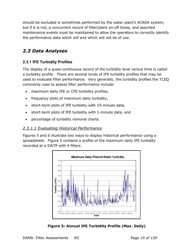
2.3.1.1 Evaluating Historical Performance
Figures 5 and 6 illustrate two ways to display historical performance using a spreadsheet. Figure 5 contains a profile of the maximum daily IFE turbidity recorded at a SWTP with 4 filters.
Figure 5: Annual IFE Turbidity Profile (Max. Daily)

DAM6: Filter Assessments SG Page 16 of 120
The chart only has the highest daily turbidity value for all four filters, and not the highest value for each filter. For this reason, the profile gives a very general idea of the performance of all the filters as a “barrier” preventing passage of pathogens. The figure shows the range of maximum daily IFE turbidity readings on a scale from 0.0 to 1.0 NTU. This type of chart can be used to compare the performance of the filters from month to month, or with a longer time-line from year to year.
An operator may also assemble a chart with the maximum daily turbidity for each filter, and use it to compare their relative performance over time. Figure 5 shows this kind of chart.
Figure 6: Comparison of Maximum Daily IFE Turbidities for Multiple Filters
The figure shows that, in this example, Filters 1, 2, and 3 generally perform better than Filter 4. Other evaluations for which this chart format might be used include comparisons of filter performance to plant production rates, comparisons of performance to changes in treatment protocols, or other unique events in the life of a filter (or plant).
Figure 7 shows another way to assemble the maximum daily IFE turbidity.

DAM6: Filter Assessments SG Page 17 of 120
Figure 7: Frequency Plot of Max Daily IFE Turbidities
In this chart, the turbidity data is presented in terms of the number of times a maximum daily turbidity was equal to or less than a value. For example, Figure 7 shows that, on 50 percent of the production days, the maximum daily turbidity was equal to or less than 0.22 NTU. All other things being equal, any change in this data point from year to year will show improved performance if the value gets lower and degrading performance if it increases.
Like the chart shown in Figure 6, this type of chart may also be used to compare the performance of individual filters or to compare plant performance from year to year.
2.3.1.2 Unit Comparisons
Figure 8 shows a chart comparing IFE turbidity, settled water turbidity, and total daily raw water pumpage.

DAM6: Filter Assessments SG Page 18 of 120
Figure 8: Chart Comparing IFE Turbidity Records to other Parameters
From January to mid-April, high IFE events seem to be paired with increases in both higher production days and higher settled water turbidity. From mid-April to June the IFE turbidity doesn’t appear to track with either of the other parameters. From June to the end of August, the IFE turbidity appears to vary with the raw water pumpage, regardless of the settled water turbidity, and from the end of November to the end of the year, the IFE turbidity trends upward with the settled water turbidity, regardless of how much water is pumped. In this example, the writer adjusted the record to create some of these trends so that each could be observed in this single figure.
However, operators commonly find one or more of these characteristics in their SWTP trend data. The fact is that weather changes contribute to fluctuations in filter performance creating a strong relationship between two parameters during one season may not be true in another. The opportunity to use these data in this way, in part, depends on the operator building a database of baseline performance, as discussed in Subsection 2.2.1.

DAM6: Filter Assessments SG Page 19 of 120
Another very revealing analysis can be the comparison of the performance of individual units. Figure 9 contains a comparison of the performance of two filters in terms of the percentage of time that each filter was on-line, the percentage of time each filter produced the highest daily maximum IFE turbidity, and the percentage of time each filter produced a maximum daily IFE turbidity above 0.5 NTU.
Figure 9: Comparing Filter Performance
In this example, both filters were on-line approximately 95 percent of the time. This suggests that only one filter was in service 5 percent of the time, but the time off-line was split between the two filters. Filters 1 and 2 produced the maximum daily IFE turbidities 15 and 85 percent, respectively. Further, Filter 2 produced water above 0.5 NTU almost twice as often as Filter 1. It may, then, be said that Filter 1 produces better water than Filter 2. Further, an operator might conclude that it is time to perform special studies to evaluate the cause of the relatively poor performance of Filter 2.

DAM6: Filter Assessments SG Page 20 of 120
2.3.1.3 Evaluating Short-Term Performance
Analyzing historical performance helps the operator identify general performance trends and/or profound changes in performance over time. Evaluating shorter-term IFE turbidity profiles can help the operator identify turbidity breakthrough events in a time frame that allows comparison to other operations data. Optimally, the filter profile will include data collected even when the filter is temporarily off-line as well as when it is in operation and discharging treated water. However, a log of the filter on/off times, filter backwashes, filtering to waste, and other events must be maintained to allow the operator to know which data is reportable and which is not.
A 15-minute sampling interval is usually not sufficient to characterize filter performance at the beginning of a production run. Filters tend to slough larger numbers of particles during the first 15 – 30 minutes of service than they do during subsequent periods of operation. Some references state that 90 percent of the particles passing through a filter do so during this startup phase of the filter run. Though not required from a regulatory standpoint, IFE turbidity levels should be recorded at least once every minute for the first 30 minutes or so.
During a mandatory Comprehensive Performance Evaluation (mCPE), TCEQ staff collected the data used to construct the chart in Figure 10 from the SWTP’s monitoring system.
Figure 10: 24-hour IFE Turbidity Profile - 15-Minute Data

DAM6: Filter Assessments SG Page 21 of 120
In the figure, we see the turbidity fluctuations detected by 15-minute IFE turbidity readings recorded on the plant’s SCADA system. “Burping” is a term used by the operators at this plant to describe a 3 to 5-minute mini-backwash cycle. The operators reportedly had to “burp” the filter, when filter production suddenly dropped, to release air that had accumulated in the filter causing air binding. The turbidimeter only detected one severe filter spike following a “burp” even though the filter was “burped” twice before it was taken off-line at 4:40 AM for a full backwash.
Figure 11 compares the 15-minute data collected by the plant’s system with the 1-minute data collected by a temporary recorder installed by TCEQ staff.
Figure 11: 24-hour IFE Turbidity Profile Comparing 15-Minute Data with One-Minute Data
As you can see, the increased monitoring frequency produced a more precise record of filter performance. The 1-minute record revealed that the second “burp” produced a spike that was almost identical in peak value to the one produced by the first burp. The difference in the duration of the two spikes was caused by the fact that the first mini-backwash lasted 8 minutes while the second only lasted 4 minutes. Further, the additional detail allowed the mCPE team to determine that the fluctuations shown in Figure 11 were cyclic, having an interval which corresponded to the operational cycles of the transfer pumps located at the filtered
DAM6: Filter Assessments SG Page 22 of 120
water transfer well. The pumps, which transfer water from the below-grade transfer well to the clearwell, would draw the water level in the transfer well down, thereby reducing the backpressure on the filtered water effluent line. Because the flow control system (that was supposed to maintain a constant filtration rate regardless of the backpressure) had failed, the variations in backpressure produced cyclic changes in the filtration rate. The fluctuating flow rate caused differences in the number of particles passing through the filter: the IFE turbidity increased and decreased exactly in time with the increases and decreases in filtration rate. The cause of the “air binding” was not determined. Even so, the constantly changing flow rate was identified as a problem that had to be eliminated.
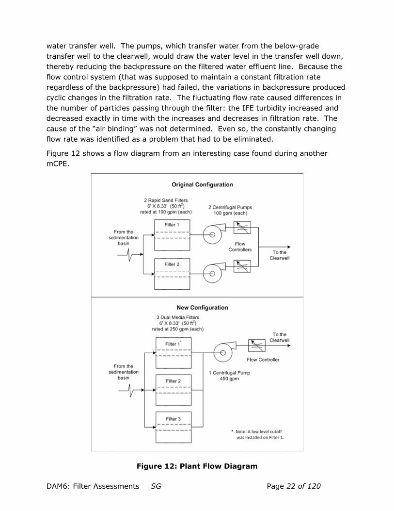
Figure 12 shows a flow diagram from an interesting case found during another mCPE.
Figure 12: Plant Flow Diagram

DAM6: Filter Assessments SG Page 23 of 120
The SWTP’s original design included two 100-gpm rapid sand gravity filters, each of which discharged to a dedicated 100 gpm transfer pump with a rate-of-flow controller (ROFC). The system owner needed more water so he added a third (identical) filter; replaced the sand with dual media; replaced the two old transfer pumps with a brand-new, much-more-efficient 450 gpm transfer pump and ROFC; and modified the filter effluent piping to accommodate the additional flow. All these modifications were made without notifying or seeking input from the system’s consulting engineer or the TCEQ. Note that the owner also failed to install a ROFC on each filter effluent line, after making the modifications.
The modification resulted in severe surges through Filter 1 as the filtered water pump would cycle on and off. Figure 13 shows the impact of the hydraulic surges on the performance of Filter 1.
Figure 13: IFE Turbidity Profile Resulting from Severe Hydraulic Fluctuations

DAM6: Filter Assessments SG Page 24 of 120
Following the modification, the owner and operators found that Filter 1 would dewater, causing the pump to cavitate. To solve the problem, the owner installed a low-level cut-off switch in Filter 1. Although the switch did prevent Filter 1 from dewatering and the pump cavitation, it did not solve the fundamental hydraulic problem or the resulting degraded filter performance.
To evaluate the problem, the mCPE team conducted a special study.2 The transfer pump was turned off, the filters were allowed to fill, and then the filter influent valves were closed. The team then turned on the transfer pump and measured the draw down rate in each filter. The team found that Filter 1 was operating at 360 gpm, Filter 2 at 70 gpm, and Filter 3 at 40 gpm. The fluctuations shown in Figure 13 show the impact the large hydraulic surges had on Filter 1. While this example represents a severe case, smaller surges still have a negative impact on filter performance, and even if the surges are very small, such as shown in Figures 10 and 11, the detectable impacts do not, as a rule, completely disappear.
Figures 15 illustrates the impact of much smaller hydraulic fluctuations on filter performance.
Figure 14: Atypical (Unusual) IFE Turbidity Profile: Flow Diagram
2 Special studies are discussed in more detail in Section 4 of this manual. This study is discussed here
only to provide a fuller description of the conditions reflected in Figures 9 and 10. Short discussions of other special studies are also presented to give more detail about some of the other figures in this section.

DAM6: Filter Assessments SG Page 25 of 120
Figure 15: Atypical (Non-typical) IFE Turbidity Profile: Turbidity Profile
The figures also illustrate the impact of intermittent filter operation and the importance of collecting data even when the filter is not in service. In this case, the hydraulic fluctuations were cause by poor pairing of the raw water pumps (i.e., the clarifier output) and the settled water transfer pumps supplying a bank of pressure filters (that are supposed to be operating at a constant rate).
During this 22-hour period, the plant was operating a raw water pump combination that had a lower output than the combination of settled water transfer pumps that were being used. Consequently, the transfer pumps would draw the clarifier down to the cutoff level, and then turn off. When the raw water pump refilled the clarifier to an adequate level, the transfer pumps would turn back on. Each time the transfer pumps restarted, the surge of flow through the filters produced a turbidity spike.
A special study revealed that the unusual rise in turbidity levels seen when the plant was not treating water resulted from the formation of manganese dioxide and aluminum hydroxide precipitates during the first 90 minutes following a production run.
The plant was applying liquid caustic (for corrosion control) and free chlorine (for disinfection) upstream of the pressure filters. Since the raw water alkalinity at this plant is quite low (i.e., often below 20 mg/L), inorganic precipitates would not form
DAM6: Filter Assessments SG Page 26 of 120
until the pH was raised and an oxidant was applied. However, these oxidation reactions proceed rather slowly and their impact was imperceptible until the plant had been off-line for at least 20 minutes. (As an aside, it should be noted that the water containing precipitates constituted only a small portion of the water produced by the plant since, when the plant was in operation, liquid ammonium sulfate is added downstream of the filters for DBP control and the LAS addition essentially terminates the oxidation reaction by converting free chlorine to monochloramine.)
Although the precipitated inorganic salts were not discernible in the CFE turbidity data collected at 4-hour intervals, they were detectable by the IFE turbidimeters at the beginning of the filter run because the filter, the influent piping, and the turbidimeter sample line and sample well would contain significant amounts of precipitate. Consequently, the severe start-up turbidity spikes, sometimes above 2.0 NTU, were seen at the beginning of each production run.
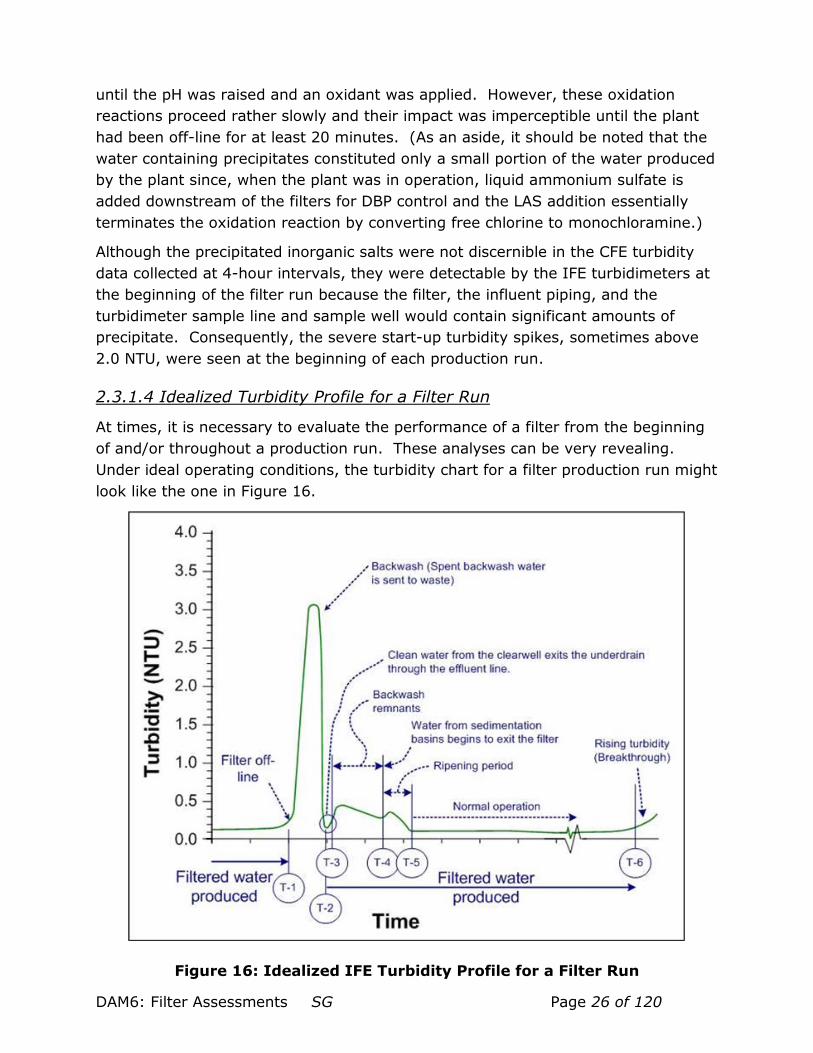
2.3.1.4 Idealized Turbidity Profile for a Filter Run
At times, it is necessary to evaluate the performance of a filter from the beginning of and/or throughout a production run. These analyses can be very revealing. Under ideal operating conditions, the turbidity chart for a filter production run might look like the one in Figure 16.
Figure 16: Idealized IFE Turbidity Profile for a Filter Run

DAM6: Filter Assessments SG Page 27 of 120
In this idealized performance chart, the different stages of the performance cycle can be seen, from the backwash all the way through to the beginning of turbidity breakthrough. In the figure, time markers, T-1 to T-6 represent different points in the filter run, as follows:
• Time-1 (T-1) is the end of a filter run and the beginning of the filter backwash.
• T-2 is the end of the backwash. At T-2, the filter is turned back on, and water from the filter effluent line begins to flow to the clearwell. (In this example there is no filter to waste.)3 The period immediately after the backwash normally has a low turbidity, because the clean backwash water pumped from the clearwell into the underdrain during the last seconds of backwash flow is emptied through the filter effluent line.
• T-3 is the time when backwash water that actually entered the media during the last seconds of backwash begins to exit the filter. There is a period of rising turbidity because this water contains high numbers of particles that were loosened from the media grains but not completely washed out with the spent backwash water.
• T-4, the second bump in the post backwash spike, occurs when the first water from the sedimentation basin finally begins to exit the filter effluent line. This part of the post-backwash turbidity spike may be larger than the first part. This second period of increased turbidity is called the ripening period. (“Ripening” is the word used to describe the process by which the individual media grains are restored to the physical and electrochemical state that produces good particle removal.)
• T-5 represents the end of the ripening process and the beginning of normal filter operation at or below the IFE turbidity level observed before the backwash.
• T-6 marks the beginning of filter breakthrough which will trigger another backwash and run cycle.
3 Filtered water compliance monitoring begins as soon as water from the filter is directed to
the clearwell and cannot be delayed until the filter has ripened or returned to normal performance.

DAM6: Filter Assessments SG Page 28 of 120
2.3.1.5 Analyzing Filter Run Data
Figure 17 contains a table showing the approximate durations of each phase of the backwash and post-backwash cycle.
Figure 17: Idealized Backwash Cycle
The times are approximate and may not be useful for assessing the backwash protocols for all filters, but they represent the normal performance of filters of typical design and loading rates.
Deviations from these times should be understood in light of the unique design characteristics or unique operations protocols. Significant unexplained differences not explained by design characteristics or operations procedures should prompt the operator to perform special studies to evaluate the cause.
Notice in Figure 17, that the settled water application rate has no direct bearing on the duration of the backwash period (T-1 to T-2). This will be determined by other parameters. Also, notice that a lower settled water application rate (2 gpm/ft2) actually prolongs the backwash spike (T-3 to T-5) because it takes longer for water carrying the loose backwash remnants to pass through the filter and it takes longer for the filter to ripen.
In order to avoid compliance issues caused by high consecutive 15-minute IFE turbidity readings, the magnitude of post-backwash turbidity spikes for lower rate filters (e.g., pressure filters) must be lower than that for higher rate filters. For example, if two consecutive IFE turbidity readings are above 1.0 NTU, a filter profile must be performed. If two consecutive IFE turbidity readings are above 2.0 NTU in two consecutive months, the system is at risk for having to request a mCPE. Historically, the design features for pressure filters do not make provision for this required lower post-backwash turbidity spike, and operators must achieve the reduction through implementation of a carefully devised backwash procedure, addition of post-backwash filter aids, or by filtering to waste.

DAM6: Filter Assessments SG Page 29 of 120
The period of normal operation (T-5 to T-6) will vary with the filter design, the settled water application rate, the quality of the settled water applied to it, and the performance parameters the operator uses to trigger a backwash.
2.3.1.6 Post-Backwash Turbidity Spikes
Figure 18 contains turbidity data collected during a mCPE conducted by TCEQ staff at a system which used pressure filters.
Figure 18: Atypical (Non-typical) Filter Backwash Spike
Because the settled water application rate allowed for pressure filters is lower than that allowed for gravity filters, the filter backwash spike was expected to last 30 to 40 minutes. In this case, the filter never did reach the performance level experienced prior to the backwash.
As the turbidity profile in Figure 18 shows, the backwash lasted 5 minutes, and the filter was allowed to sit idle for about 22 minutes. When the plant was turned back on, it took 65 minutes for normal turbidity levels (levels below 0.3 NTU) to be established. There was essentially was no period when clean water from the

DAM6: Filter Assessments SG Page 30 of 120
clearwell was discharged from the filter underdrain, it took 25 minutes to wash the backwash remnants from the filter, and it took another 40 minutes for the filter to ripen to the point where water below the 0.3 NTU level was produced again. At 90 minutes after filter startup, the IFE turbidity was still higher than the pre-backwash turbidity level.
The turbidity profile in Figure 18 would alert a knowledgeable operator to the following:
(1) Fact: The post-backwash turbidity spike peaks at above 3.0 NTU and the spike remained above 2.0 NTU for about seven minutes.
(2) Fact: If the spike were to be further prolonged, the system would be at risk for having a confirmed reading above 2.0 NTU.
(3) Fact: Though there was a brief period of lower turbidities, the filter continued to produce water above 1.0 from about 15:02 hours to around 15:57 hours. Even with the intermittent period of reduced turbidity, the system does have a confirmed IFE turbidity reading above 1.0 NTU.
(4) Fact: The five minutes of backwash flow does not appear to produce the desired results. Clearly, when the backwash water is turned off, the 3.0 NTU spike contains too many remaining particles to call the filter “clean”.
(5) Conjecture: The very long ripening period suggests that the operator might want to consider addition of a filter aid immediately after filter startup to shorten the ripening period.
(6) Conjecture: The lack of the short period when clean clearwell water in the underdrain passes through the effluent line suggests that there is a leaking valve, and this cleaner water is leaving the filter during the 22 minutes while it is supposed to be idle. While this is conjecture, this type of finding in a filter profile should provoke one or more special studies and/or a maintenance activity to see if this problem can be eliminated.
There may be many other design and operational considerations that may indicated, conclusions that may be drawn, or conjectures that might be made regarding the shape of the post-backwash turbidity spike, but this example illustrates how one might begin evaluating post-backwash turbidity data.
2.3.1.7 Percentage of Turbidity Removal
Another useful analysis is to calculate and plot the percentage of turbidity (or particle) removal by a filter over time (Figure 19).
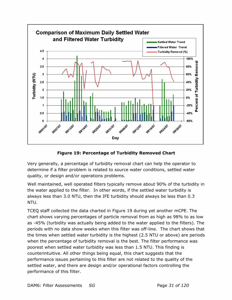
DAM6: Filter Assessments SG Page 31 of 120
Figure 19: Percentage of Turbidity Removed Chart
Very generally, a percentage of turbidity removal chart can help the operator to determine if a filter problem is related to source water conditions, settled water quality, or design and/or operations problems.
Well maintained, well operated filters typically remove about 90% of the turbidity in the water applied to the filter. In other words, if the settled water turbidity is always less than 3.0 NTU, then the IFE turbidity should always be less than 0.3 NTU.
TCEQ staff collected the data charted in Figure 19 during yet another mCPE. The chart shows varying percentages of particle removal from as high as 98% to as low as -45% (turbidity was actually being added to the water applied to the filters). The periods with no data show weeks when this filter was off-line. The chart shows that the times when settled water turbidity is the highest (2.5 NTU or above) are periods when the percentage of turbidity removal is the best. The filter performance was poorest when settled water turbidity was less than 1.5 NTU. This finding is counterintuitive. All other things being equal, this chart suggests that the performance issues pertaining to this filter are not related to the quality of the settled water, and there are design and/or operational factors controlling the performance of this filter.
DAM6: Filter Assessments SG Page 32 of 120
2.3.1.8 Other Analyses
There are several other analyses that an operator can execute using filter performance records, and operators should not hesitate to develop those data comparisons that will serve best for determining the filter’s performance status. Examples of other comparisons that might be useful to an operator include, are not limited to comparing IFE turbidity data to:
• head loss trends,
• pump on/off status,
• increasing or decreasing filter loading rates,
• improved or degraded sedimentation basin performance, and
• turbidity profiles while adjacent filters are backwashed.
2.3.2 Analyzing Head Loss Trends
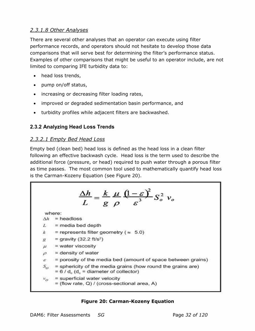
2.3.2.1 Empty Bed Head Loss
Empty bed (clean bed) head loss is defined as the head loss in a clean filter following an effective backwash cycle. Head loss is the term used to describe the additional force (pressure, or head) required to push water through a porous filter as time passes. The most common tool used to mathematically quantify head loss is the Carman-Kozeny Equation (see Figure 20).
Figure 20: Carman-Kozeny Equation

DAM6: Filter Assessments SG Page 33 of 120
Zero head loss is defined as the empty bed head loss. Before operators can evaluate empty bed head loss trends, they must understand the relationship between all of the variables that affect flow in a porous media filter. While most of us do not need a full and detailed understanding of the Carman-Kozeny Equation, we need to understand the impact of water and media properties on filter operation.
The table in Figure 21 shows, very generally, the factors in the Carman-Kozeny Equation, and their impact on head loss.
Figure 21: The Factors in the Carman-Kozeny Equation

DAM6: Filter Assessments SG Page 34 of 120
The factors in the Carman-Kozeny equation are as follows:
• Bed Depth: The deeper the media bed, the more the head loss through the filter.
o In a deeper filter bed, there will be more friction loss than in a shallow filter because there are more media grains (and therefore more surface area) in the deep filter.
o In a deeper filter bed, there is more time for the flow resisting effects of viscosity to increase the filter head loss.
• Geometry Factor: The filter geometry factor can be thought of as a “correction factor” and is estimated to have a value of 5.0.
• Gravity: Gravity is the attractive force applied by the earth to the water which causes it to flow downward through the filter.
• Viscosity Factor: Water viscosity is a measure of a fluid’s internal resistance to flow. The higher the viscosity value, the more the fluid resists flow.
• Water Density: Water density is a measure of how much the force of gravity draws the water downward: the higher the density, the greater the pull of gravity on a volume of water.
• Water Temperature: Temperature is not a factor in the Carman-Kozeny equation, but it affects both density and viscosity. The higher the temperature, the less the head loss through the filter.
o Increasing the temperature reduces the density of the water, reducing the downward draw of gravity per unit volume of water.
o Increasing the temperature also reduces the water’s viscosity, and it’s resistance to flow.
o Because raising the temperature reduces the viscosity of water to a proportionally greater degree than it reduces its density, raising the temperature results in a lower head loss.
• Media Bed Porosity: Porosity is the measure of the volume of the spaces between filter grains and it depends on the size and shape of the media grains. The higher the porosity, the more space (volume) and the lower the head loss through the filter.
o Small, round grains will pack together much more tightly than larger or more irregularly-shaped grains.
o As media wears, the grains become smaller and more spherical. Therefore, a filter bed containing worn media grains will produce a higher empty bed head loss than a bed containing media that is in pristine condition.

DAM6: Filter Assessments SG Page 35 of 120
o The actual porosity of the filter bed is also dependent on how much of the space between the grains has been filled with floc and other particles. If the bed has been thoroughly backwashed, the amount of previously collected particles filling the pores will be lower than if the bed has not been thoroughly backwashed. Therefore, a higher empty bed head loss can be an indicator of poor backwash technique.
• Sphericity Factor: Sphericity is a measure of the roundness of the filter grains. It is directly related to the tendency of the media to pack tightly or to maintain void spaces between the grains.
• Media Size: Large media grains accrue less head loss that smaller media grains.
o Large grains have less surface area per unit volume than smaller media grains. Since the amount of surface area affects how much energy is lost to friction, large media grains produce lower head losses than small media grains.
o As media grains break down, they become smaller (increasing the surface area per unit volume) and produce more head loss due to increased friction and reduced porosity.
o On the other hand, the grains can become appreciably larger if they get coated with organic or inorganic materials. However, this cannot be directly correlated to decreased head loss, because these coatings also increase sphericity and decrease porosity.
• Specific Velocity/Filtration Rate: Specific velocity is the flow rate divided by the cross-sectional area though which it flows.
o The higher the filtration rate, the greater the head loss.
o Head loss increases directly with the flow rate through the filter because the faster flowing water produces more friction than slow moving water.
o Additionally, the higher the filtration rate, the more impact the viscosity has on the head loss.

DAM6: Filter Assessments SG Page 36 of 120
Generalizing all the above information, the Carman-Kozney equatiion can be represented as shown in Figure 22.
Figure 22: Simplified Representation of the Carman-Kozeny Equation
Very generally:
• a well-backwashed filter will have a lower initial head loss than a filter that has not been backwashed adequately;
• a operating at a low filter loading rate will have lower head loss than one operating at a high filter loading rate;
• increases or decreases in empty bed head loss indicate that something has changed in the filter bed. For example:
o a rapid and unexpected increase in empty bed head loss can indicate air binding,
o a gradual increase in the empty bed head loss can result because the media grains are changing size or shape.
2.3.2.2 Filter Run Head Loss
If particles are accumulating throughout the entire depth of the filter bed, head loss tends to increase linearly over time, at least until the filter has collected so many particles that the size of the pores between the media grains begin to shrink at a proportionally higher rate. Turbidity breakthrough occurs before the pores in the filter bed completely fill with particles.
Figure 23 shows a representation of settled water flowing through clean media and dirty media.

DAM6: Filter Assessments SG Page 37 of 120
Figure 23: Flow Through Clean vs. Dirty Media
As the pores fill with particles, the empty pore volume gets smaller. Since the empty pore volume decreases, when a filter is operating in a constant rate mode, the water velocity has to increase because there is less room for the water to move through. At the higher velocity, shear forces cause the friction between the water and the floc particles to increase and as these forces rise, they strip previously deposited particles off the filter grains the loosened particles then pass through to the underdrain. Consequently, the effluent turbidity level begins to rise.
On the other hand, water treatment plants sometimes see a significant increase in head loss long before particle breakthrough if the head loss is occurring in the floc mat that forms on the surface of the media or in the top few inches of the filter bed. This effect is sometimes called “surface blinding”. This effect is illustrated in Figure 24.

DAM6: Filter Assessments SG Page 38 of 120
Figure 24: Filter Head Loss vs. Filter Run-Time
If surface blinding occurs, the head loss will increase at a faster rate but turbidity breakthrough will not occur because particles that are sheared from the top of the filter can still be trapped at a point deeper in the filter bed. Surface blinding is important because, in severe cases, it can result in a low-pressure zone at a deeper point in the filter bed.
Figure 25 shows a representation of the water pressure at different depths of water flowing through a media bed.
Figure 25: Pressure at Depth for Multiple Filter Run Volumes

DAM6: Filter Assessments SG Page 39 of 120
The line running diagonally from 3.5 on the y-axis, to 3.5 on the x-axis, shows what the head would be if there were no media in the filter or if the water in the filter was still (not flowing). The black hashed area represents the water pressure that is lost due the friction of the water flowing through the media. Note that the head loss increases
proportionally (linearly) with depth when the filter is clean. The colored areas represent the head loss at increasing depths after filtering increased volumes of settled water: Volume-1 (v1), Volume-2 (v2), and Volume-3 (v3). These pressure lines are not proportional with depth, because the deposition of floc in the filter bed is not truly linear with depth.
As shown in Figure 25, if the pressure in the filter bed drops low enough, dissolved air can begin to come out of solution and form air pockets in the media. Though some of the air will escape during the filter run, the air pockets can disrupt the water flow in the filter because the water has to flow around the air pocket rather than through the voids the pocket has engulfed. This effect is called air binding and, in severe cases, can suddenly and drastically reduce filter output.
2.3.3 Analyzing Filter Productivity Trends
There are several ways to track filter productivity. One of the simplest methods is to keep track of the number of hours that a filter can be run before one of the backwash triggers (i.e., IFE turbidity, head loss, etc.) has been exceeded. Although this method is useful when the filters are all the same size and operate at the same flow rate all of the time, it may not be that useful when the plant has different sizes of filters or changes in the flow rate through each filter depending on consumer demand.
2.3.3.1 Unit Filter Run Volume
Tracking the Unit Filter Run Volume (which measures the volume of water filtered through each square foot of the media surface over the course of an entire run, see Figure 26) is a more useful measure at most plants because it normalizes (adjusts) the filter production data based on both filter size and filter loading rate.

DAM6: Filter Assessments SG Page 40 of 120
Figure 26: Unit Filter Run Volume
If all of the filters are exactly the same size, the plant does not have to compensate for size and can, therefore, use the Filter Run Volume instead.
Temporary (short-term) changes in UFRV can be caused by several factors, such as fluctuations in raw water quality, changes in settled water turbidity levels, or inconsistent backwash techniques.
However, changes which take a long term to develop may be due to some form of filter damage. For example, gradual declines in the UFRV can result from premature turbidity breakthrough, underdrain damage, or excessive backwash water flow rates which result in media loss. Any appreciable unexplained change in the UFRV trend should be investigated.
Although the UFRV does compensate for filter area and filtration rate, it still provides a less than complete assessment of filter productivity because it does not consider the amount of backwash water it takes to keep the filter clean. There are two methods that are commonly used to evaluate filter efficiency, normalized net yields and percent net yield.
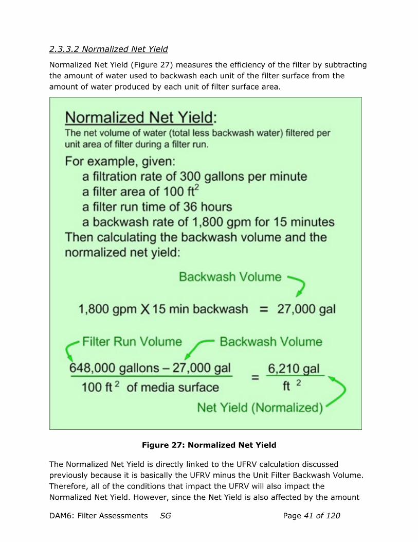
DAM6: Filter Assessments SG Page 41 of 120
2.3.3.2 Normalized Net Yield
Normalized Net Yield (Figure 27) measures the efficiency of the filter by subtracting the amount of water used to backwash each unit of the filter surface from the amount of water produced by each unit of filter surface area.
Figure 27: Normalized Net Yield
The Normalized Net Yield is directly linked to the UFRV calculation discussed previously because it is basically the UFRV minus the Unit Filter Backwash Volume. Therefore, all of the conditions that impact the UFRV will also impact the Normalized Net Yield. However, since the Net Yield is also affected by the amount
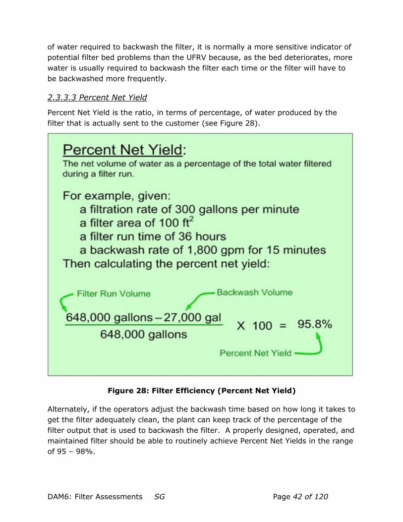
DAM6: Filter Assessments SG Page 42 of 120
of water required to backwash the filter, it is normally a more sensitive indicator of potential filter bed problems than the UFRV because, as the bed deteriorates, more water is usually required to backwash the filter each time or the filter will have to be backwashed more frequently.
2.3.3.3 Percent Net Yield
Percent Net Yield is the ratio, in terms of percentage, of water produced by the filter that is actually sent to the customer (see Figure 28).
Figure 28: Filter Efficiency (Percent Net Yield)
Alternately, if the operators adjust the backwash time based on how long it takes to get the filter adequately clean, the plant can keep track of the percentage of the filter output that is used to backwash the filter. A properly designed, operated, and maintained filter should be able to routinely achieve Percent Net Yields in the range of 95 – 98%.

DAM6: Filter Assessments SG Page 43 of 120
2.4 Data Analysis Summary There is a great deal of data which a SWTP must collect, assemble and store each day of operation. Above that, much of this data must be reported to regulatory agencies and must be available for review during periodic inspections. The performance history represented by these data must confirm regulatory compliance, but with only a modest bit of organization and spreadsheet analysis they can be used for much more than that.
Other routinely gathered operations information, coupled with the compliance data, can be used by the operator to measure filter performance in clearly understandable terms. Further, they can be used to predict and/or identify performance problems, and with considered application, the data can also be used by the operator to achieve the most cost effective and/or optimized treatment.
The preceding discussion of data analysis involves less “math” than calculating a chemical dose based on a jar test. This section is only intended to provide a starting point for the operator to see the usefulness of evaluating data that is already being collected. Once the processes for presenting the data in an interpretable format are established, it takes less time to maintain up-to-date analyses than it takes to try to solve a filter performance problem essentially by trial and error or to work around a filter problem by using more backwashes and shorter filter runs.

DAM6: Filter Assessments SG Page 44 of 120
Section 3: Routine Observations and Maintenance
3.1 Routine Visual Observations Just looking at a filter can provide qualitative information that operators need to determine if more complex special filter studies are warranted. If possible, once each week, operators should visually observe the backwash from the time the filter is taken out of service to the time that the backwash is completed. If that rigorous level of observation is not possible, operators should watch each filter being backwashed at least once each month or two. Observing how the filter responds before and during the backwash process not only allows operators to detect problems with the backwash system and procedure, it allows them to inspect the surface of the filter bed so that they can evaluate the condition of the filter and, indirectly, the underdrain and support system.
3.1.1 Air Releases
One anomaly that may be observed during a backwash is the emergence of air. As noted previously, small air bubbles can form within the filter bed when floc builds up on or near the surface of the filter bed. If the bubbles become large enough, they can interfere with flow of water in the filter. In severe cases, an air pocket can grow large enough to significantly reduce filter output, a condition known as air binding.
Operators should periodically check each filter for signs of air entrainment. Although air bubbles can sometimes be observed when the filter is in operation, they are easier to detect when the filter is taken off-line and partially-drained in preparation for a routine backwash. During normal operation, the downward flow of the water tends to keep small bubbles from escaping from the filter bed. However, there is no downward flow when the filter is taken off-line. Under these conditions, it is easier for the entrained air to escape and be observed.
Air bubbles are also sometimes observed when backwash water is introduced into the bottom of the filter at the beginning of the backwash cycle. These “backwash releases” may not be caused by air entrainment in the filter bed; they may be caused by leaking valves or some similar problem that allows the backwash supply line to partially or fully dewater between backwash cycles. Air pockets form at the highest points in the partially dewatered line and, when the backwash process is initiated, they are discharged into the filter underdrain and enter the filter bed. While small volumes of air probably cause little damage, larger volumes of air can dislodge the underdrain components and disturb the gravel support layer in filters not designed for air scour.

DAM6: Filter Assessments SG Page 45 of 120
3.1.2 Changes in Media Depth
The depth of the filter bed may change over time. Regardless of whether the change is rapid or slow, the change in depth will eventually cause a change in filter performance. A gradual decline might be due to media degradation or media loss during backwash. A gradual increase may be due to media grain encrustation and/or mudball accumulation. Rapid changes in bed depth are usually associated with severe underdrain damage or grossly inappropriate backwashing practices. All sudden changes in bed depth need to be investigated at the earliest possible time.
Figure 29 shows a filtered water transfer tank serving a bank of four filters.
Figure 29: Filtered Water Transfer Tank with Sand and Anthracite
The gravel layers in all four filters had been disrupted by excessive backwash pressures and flow rates, and the media began to wash out through the underdrain. The operators observed that the surface of the media was going down, but assumed anthracite was being carried out during backwash. In response, the operators periodically added more anthracite to the filters and reduced the backwash flow rate to the point of making the backwash ineffective.

DAM6: Filter Assessments SG Page 46 of 120
However, no matter how much the reduced the backwash rate, they continued to lose media. What the operators could not see is that the sand was disappearing too. By the time they discovered that their media was washing into the transfer tank, almost all the sand had been lost and the filter bed was almost totally anthracite. Had the loss of media been occurring during the backwash, media would most likely have been seen overflowing the backwash trough.
Losses of more than 2 or 3 inches can reduce filter run times and net yields, and require corrective action. Although changes of 1 – 2 inches will probably have no significant impact on filter performance, they may also warrant further investigation. Properly-operated plants with dual media filters may see an average anthracite loss on the order of 5 – 7% per year so the filter may need to be capped with additional anthracite every 2 – 3 years to maintain a consistent performance level.
An increase in the bed depth is less common. Therefore, operators should conduct one or more comprehensive special studies (discussed in Section 4 of this manual) if there is any appreciable increase in bed depth.
Often, it is possible to detect changes in the elevation of the media bed by visually “marking” the surface of the media against the filter wall and checking it just before the backwash procedure begins. However, more quantitative assessments are easy to conduct by measuring the distance from the top of the media bed to a fixed reference point, e.g., the top of the filter wall. Since the top of the filter wall and the top of the underdrain are at fixed elevations, the depth of the media bed has decreased if the distance between the top of the wall and the top of the filter bed has increased.
3.1.3 Mudballs
Over the course of a filter run, media grains become coated with floc, dirt, and other particles. Although an effective backwash process removes most of this coating, it is not desirable to remove it completely. A small residual coating contributes to effective filtration during the post-backwash period by reducing the time it takes the filter to ripen.
However, an ineffective backwash will leave the grains coated with excess dirt and coagulant and if the coating becomes too thick, water and media pressure causes the grains and attached floc to compact forming a solid mass, called a mudball (see Figure 30).

DAM6: Filter Assessments SG Page 47 of 120
Figure 30: Mudball Effects
Once a mud ball is formed, it will tend to grow, consuming more and more filter grains and more filter bed volume. As the mudball increases in size, the ratio of the weight relative to mudball surface area also increases. Since the mudball surface is where the friction of the backwash water lifts the mudball toward the backwash trough and the weight is what tends to force it downward, a growing

DAM6: Filter Assessments SG Page 48 of 120
mudball will become less and less likely to be washed out and will settle deeper and deeper into the filter bed during backwashes.
The clogging of media with mudballs has several effects:
• Large numbers of mudballs interfere with the uniform flow of water through the surface of the media bed during normal operation and during backwashing. Therefore, less of the filter surface area is available to filter water.
• As the available filter surface area becomes smaller, filter head loss increases due to the increased settled water velocities through the remaining unblocked media. These increased velocities contribute to particle breakthrough and shorter filter runs.
• Clogged media tends to contract and as mudball formation progresses, cracks will form in the media. The cracks result in short-circuiting and degraded filtered water quality. (This issue will be discussed in more detail in Subsection 3.1.5.1, below.)
Although it is very difficult to completely prevent mudball formation, it is important to prevent the accumulation of excessive numbers of small mudballs and, if necessary, to remove the mudballs before they grow large enough to interfere with filter operation. In order to prevent filter problems and to prolong the life of the media, mudballs should be removed if they cover more than 5% of the bed surface or become larger than ½-inch in diameter or more than ¼-inch thick.
3.1.4 Filter Backwash Irregularities
3.1.4.1 Ideal Backwash Flow
The filter backwash process may be automated or entirely controlled by manual operator adjustments. However, in general, the goals of the filter backwash are to remove particles collected in the media, to restratify the media for the next filter run, to avoid passing particles in excessive numbers during or immediately after the backwash, and to do all this without damaging the filter. In order to accomplish these goals, the backwash air and water must be distributed uniformly across the entire filter bed.
Figure 31 shows an idealized representation of this condition.

DAM6: Filter Assessments SG Page 49 of 120
Figure 31: Idealized Dispersion of Water During Backwash
Backwash water enters beneath the filter through nozzles, slots, or holes in the underdrain, passes through the support gravel (if present), and enters the media bed. Regardless of whether or not the filter uses a gravel support or gravelless system, the media support system is designed disperse the backwash water across the footprint of the filter, creating a very uniform flow through the media bed.
As the backwash flow rate increases, the effect of the lift on the media causes fluidization of the media (see Figure 32).
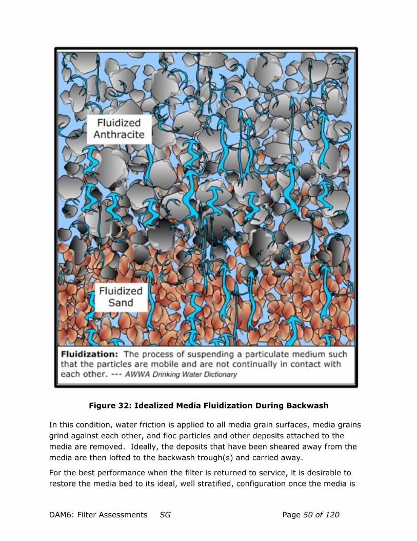
DAM6: Filter Assessments SG Page 50 of 120
Figure 32: Idealized Media Fluidization During Backwash
In this condition, water friction is applied to all media grain surfaces, media grains grind against each other, and floc particles and other deposits attached to the media are removed. Ideally, the deposits that have been sheared away from the media are then lofted to the backwash trough(s) and carried away.
For the best performance when the filter is returned to service, it is desirable to restore the media bed to its ideal, well stratified, configuration once the media is

DAM6: Filter Assessments SG Page 51 of 120
clean. “Well stratified” means that there are well defined media layers with the smallest possible interface between consecutive layers of different media4.
The agitation of the media bed by the air scour and/or backwash water will, of course, have a tendency to cause mixing of the media during the backwash. Fortunately for the operator, anthracite normally fluidizes at a backwash flow rate of 7 to 8 gpm/ft2 while sand fluidizes at a backwash flow rate of about 11 to 12 gpm/ft2.
Consequently, once the filter is clean, the operator may reduce the backwash flow long enough to allow the sand to settle (say to less than 10 gpm/ft2, and after the heavier media has settled, the backwash flow may be further ramped down to allow the anthracite to settle. This is most often accomplished by a gradual reduction in the backwash flow rate from full flow to zero flow rather than by “stair-stepping” the flow down.
3.1.4.2 Unreliable Surface/Subsurface Wash
Filters equipped with surface or subsurface wash facilities may develop problems as they get older and experience wear. Stationary surface wash mechanisms have fewer maintenance issues than rotating mechanisms but develop some of the same problems. Auxiliary wash problems may decrease the effectiveness of the filter backwash and result in shortened media life, shortened filter run times, mudball formation, and higher filter run turbidities.
Specific items to look for, and repair if necessary, include:
• Uneven dispersal of the surface wash on the media surface is an indication of degraded nozzle performance. Spray nozzles may clog or rust away changing the way that the water is delivered to the surface of the media.
• Surface wash arms (agitators) hanging on the media or other mechanical fixtures as they rotate may be an indication that the media depth is increasing (indicating other problems), the media surface is not level, the bearings are failing, or the structural integrity of the surface wash mechanism is failing.
• Wash arm bearings that squeal or grind, or sluggish rotation of the wash arms are an indication that the bearings may need to be replaced or serviced.
4 Please be aware that engineering schools and technical references once taught that a thick
anthracite/sand interface layer would improve filter performance, but extensive recent studies have shown that this is not the case. Still, there are a lot of industry references that have not been modified to reflect this new information.

DAM6: Filter Assessments SG Page 52 of 120
• Inadequate spray volume or spray pressure to effectively break up the media surface is an indication that the surface wash water supply or delivery system has become unreliable or the media is becoming compacted during the filter run.
• Leaking surface wash plumbing, such as leaking or missing end caps, demonstrates a degrading ability to achieve the desired media penetration and loosening of floc and other particles attached to the media.
• The nozzles of subsurface wash mechanisms are more subject to becoming clogged with media than the nozzles on surface wash mechanisms.
• As with any mechanism where filtered water plumbing comes in direct contact with settled water, the backflow preventer serving the surface wash mechanism should be inspected regularly and confirmed to be functioning, and repaired, if necessary.
3.1.4.3 Irregular Air and Backwash Water Distribution
Backwash facilities must provide enough energy to shear the floc coating away from the media grains. Because the media will be lifted by the rising backwash flow, the most energy that can be applied to any grain is approximately equal to the buoyant weight of that grain. In order to adequately backwash the filter, all regions of the media bed must receive enough backwash water to apply this energy to the media at all locations.
Therefore, the filter support system is designed and constructed to receive the backwash air and water and distribute it equally to all areas of the filter. If a gravel support system is not level, if there are high and low places in the media, or if there is underdrain damage there will be regions with more or less resistance to the backwash air flow and/or the backwash water flow (see Figure 33).
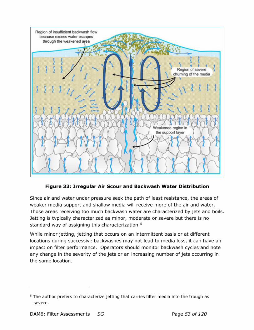
DAM6: Filter Assessments SG Page 53 of 120
Figure 33: Irregular Air Scour and Backwash Water Distribution
Since air and water under pressure seek the path of least resistance, the areas of weaker media support and shallow media will receive more of the air and water. Those areas receiving too much backwash water are characterized by jets and boils. Jetting is typically characterized as minor, moderate or severe but there is no standard way of assigning this characterization.5
While minor jetting, jetting that occurs on an intermittent basis or at different locations during successive backwashes may not lead to media loss, it can have an impact on filter performance. Operators should monitor backwash cycles and note any change in the severity of the jets or an increasing number of jets occurring in the same location.
5 The author prefers to characterize jetting that carries filter media into the trough as
severe.

DAM6: Filter Assessments SG Page 54 of 120
As Figure 34 indicates, severe backwash jets create a rolling flow pattern that looks like a spot of boiling media in the filter.
Figure 34: Photograph of Severe Jetting
At the site where the boil is located, the gravel bed/support structure is disrupted. As a result, the media will reach incipient fluidization (i.e., the condition where the upward velocity needed to begin lifting the media is reached) sooner at this location than in other parts of the filter. The rapidly rising water draws media into the jet at the point where it leaves the gravel/support system much like an eductor draws chlorine from a chlorine cylinder. Then you get a rolling boil like the one shown in the photograph in Figure 34.
As discussed earlier, a poorly constructed underdrain or a poorly constructed gravel support layer can cause jetting of backwash air and water. However, a properly constructed filter can be damaged by opening the backwash air/water valves too quickly.
The TCEQ did a mandatory CPE at a facility where an untrained weekend operator backwashed all the filters, turning on the air scour at full flow at the start of every backwash. In doing so, he disrupted the underdrain of five of the six filters, which

DAM6: Filter Assessments SG Page 55 of 120
began losing filter media to the clearwell. Subsequent to this event, jets were noticeable during all phases of the filter backwash. Care must be taken to never challenge a filter with too much air or too much backwash flow.
Figure 35 provides a cross-sectional representation of a filter with severe underdrain damage.
Figure 35: Sectional View of Severe Jetting
Underdrain or support system damage will result in severe jets and boils. As shown in Figure 35, more filter media tends to accumulate in portions of the filter which are not being “jetted” while less filter media settles in the areas with a lot of jetting, one cause for mounds and depressions in the media bed.

DAM6: Filter Assessments SG Page 56 of 120
3.1.4.4 Backwash Trough Construction
It is important to make sure that the tops of all the troughs are at the same elevation. Uneven troughs can produce irregular flow patterns during the backwash process. The upward component of backwash water flow fluidizes the media, and lifts the floc. However, it is the lateral component of the backwash flow that carries the rising floc to the trough and out of the filter box. Spent backwash water and the floc carried by it will tend to flow toward and into the lowest section of trough rather than to the nearest section of trough. Longer backwashes are often needed to remove the floc that has to travel a longer distance from to reach a section of trough that is actually receiving water.
Although there are more sophisticated techniques for evaluating the levelness of the backwash troughs, visual observations provide a very sensitive means of determining whether or not they are level. Observe the water level as the filter is drained before a backwash, if the top of the troughs are level; the water drops to the tops of each section of trough at the same time. A second observation can be made as the water level rises again when the backwash process is started, i.e., if the troughs are level, spent backwash water will begin flowing over all portions of the troughs at the same time. Figure 36 shows examples of filters where portions of the troughs are receiving backwash water while other portions are not.
Figure 36: Examples of troughs that are not level
Although undersized backwash troughs and spent backwash water piping can cause flooding, as is the case in Figure 37, the most common causes are a faulty backwash waste valve or a high water-level in the spent backwash water tank or lagoon.

DAM6: Filter Assessments SG Page 57 of 120
Figure 37: Examples of Trough Flooding
Both of these common causes increase the backpressure on the backwash waste line which causes the spent backwash water to back up in the filter box.
3.1.5 Media Surface Irregularities
3.1.5.1 Retraction
As noted in the previous section, a thick floc layer on the filter grains can cause the formation of mudballs. However, excess floc can also prevent the filter media from settling properly and cause cracks and voids to form between the solid mass and surrounding the filter medium or filter wall. Retraction cracks usually develop first along the edges of the filter as the mass retracts from the filter wall. However,
when the problem becomes more severe, cracks develop in other locations as well. The right hand photo in Figure 38 show a solid layer of floc on the surface of the media, but the retraction cracks are also plainly visible. Though the cracks are narrow, they are deep and provide an unfiltered path to the depths of the filter bed and/or the underdrain. Since water under pressure seeks the flow path of least resistance, these cracks can pass a lot of unfiltered water.

DAM6: Filter Assessments SG Page 58 of 120
In the early stages, these defects are difficult to see unless the water is drawn down to the point where it is just above (or even just below) the surface of the media.
Therefore, operators should partially drain the filter once, maybe twice, each year for a cursory visual inspection. Since a filter traps large amounts of floc over the course of the filter run, it is probably best to evaluate this type of problem following, rather than before, a backwash cycle to make it easier to distinguish between problems that will be alleviated by a routine backwash and those that will remain and cause long-term problems.
Figure 38: Retraction Cracks
Post-backwash retraction cracks that are more than about ½-inch wide, more than about 1-inch deep, or more than a few inches long indicate that special filter studies may be needed to evaluate the condition of the filter bed and media grains. While less severe problems may not warrant special studies, they do indicate the need to closely observe the backwash water flow in the area where the cracks are detected to make sure that those areas of the filter are adequately cleaned during the filter backwash cycle.
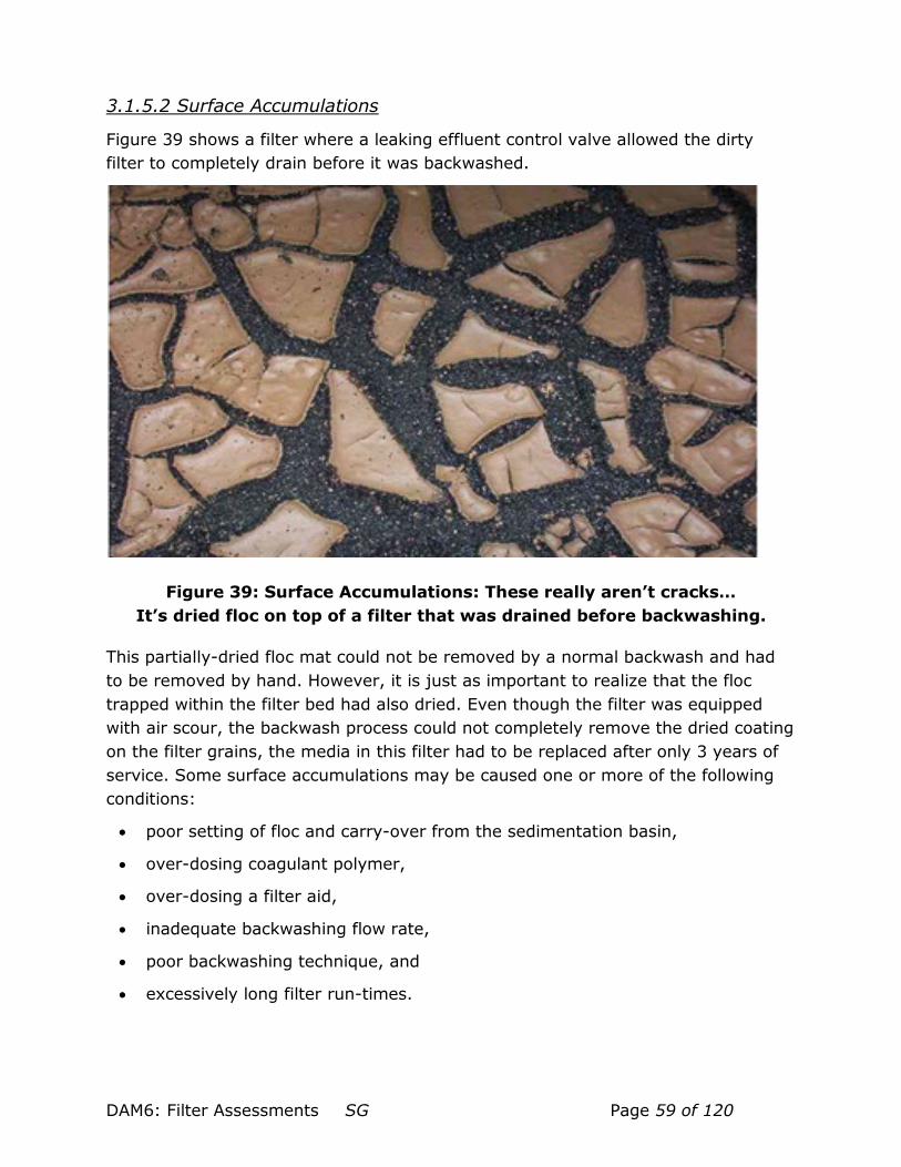
DAM6: Filter Assessments SG Page 59 of 120
3.1.5.2 Surface Accumulations
Figure 39 shows a filter where a leaking effluent control valve allowed the dirty filter to completely drain before it was backwashed.
Figure 39: Surface Accumulations: These really aren’t cracks… It’s dried floc on top of a filter that was drained before backwashing.
This partially-dried floc mat could not be removed by a normal backwash and had to be removed by hand. However, it is just as important to realize that the floc trapped within the filter bed had also dried. Even though the filter was equipped with air scour, the backwash process could not completely remove the dried coating on the filter grains, the media in this filter had to be replaced after only 3 years of service. Some surface accumulations may be caused one or more of the following conditions:
• poor setting of floc and carry-over from the sedimentation basin,
• over-dosing coagulant polymer,
• over-dosing a filter aid,
• inadequate backwashing flow rate,
• poor backwashing technique, and
• excessively long filter run-times.

DAM6: Filter Assessments SG Page 60 of 120
3.1.5.3 Mounds and Depressions
The photograph in Figure 40 shows a filter that had been in operation for about 20 hours before it was taken off-line and drained for a filter inspection.
Figure 40: Mounds and Depressions (1)
This filter had been retrofitted with a new underdrain and air scour system less than 24 months prior to our inspection. The photo shows a severe (23-inch deep and 24-inch wide) depression at one of the connections between the air supply header and the underdrain. The depression was surrounded by a 2-inch high media mound that extended about 12-inches from the perimeter of the depression (although the only visible indication of the mound is the accumulation of floc in the lower right hand corner of the image).
The filter contained a severely disrupted gravel layer but the inspectors could not determine if the depression was caused by a leaking air line connection or a damaged underdrain because they did not want to excavate the gravel layer. However, following the inspection, the filter was refilled and then backwashed. During the backwash cycle, the team observed excessive air flow (during the air-scour stage) and excessive water flow (during the water-only backwash stage) in the area of the depression and the depression continued to be present following the backwash cycle although it was not nearly as severe.

DAM6: Filter Assessments SG Page 61 of 120
Prior to the backwash the media layer at the bottom of this depression contained 9 inches of anthracite and no sand. Therefore, the head-loss in this area is much lower than the head-loss in the rest of the filter (which contained approximately 8 inches of sand and 24 inches of anthracite although the original specifications called for 12 inches of sand and 24 inches of anthracite). This finding confirms that sand was being flushed through the underdrain during the filter run.
As a result of the bed damage, much more water will flow through the area where the depression is located (due to a much lower head-loss). In addition, both the filter grain surface area and pore volume in this part of the filter was much lower, which was contributing to the extremely short filter runs prior to turbidity breakthrough.
Figure 41 shows a photo of another depression in the same filter after the same 20-hour filter run.
Figure 41: Mounds and Depressions (2)
This depression was located near the center of the filter and was about 9-inches in diameter and about 8 inches deep.
Unlike the depression shown in the previous image, this depression was surrounded by a concentric gradual decline in the surface elevation that extended as far as 18-

DAM6: Filter Assessments SG Page 62 of 120
inches from the center of the hole. Notice that the floc deposits in the center of the depression are heavier than in the surrounding area; this is an indication that more water is passing through the bottom of the depression than through the surrounding filter area.
During the post-inspection backwash cycle, the team again observed excessive air and water flow (jetting) at the site of the depression. However, there was no evidence of a depression following the filter backwash. The backwash leveled the media above the damaged underdrain, but when the filter was returned to normal operation, media began to wash through the underdrain and the crater reformed in the same location. This finding suggests that the underdrain system at this site is seriously damaged.
Figure 42 shows two drawings:
• one depicting the cross-section of a media bed after backwashing, and
• the other with a cross-section of the media bed after media has been washed through the underdrain during a filter run.
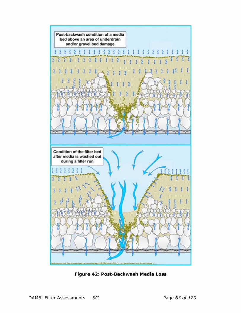
DAM6: Filter Assessments SG Page 63 of 120
Figure 42: Post-Backwash Media Loss

DAM6: Filter Assessments SG Page 64 of 120
The figure shows that the severe disruption of the media support system (in this case gravel) allows sand to be washed into the underdrain.
3.1.6 Filter Box Cross Connections
Cross-connections associated with the filter box or filter piping are an important issue because the integrity of the filtered water must be protected from possible contamination with settled water or other waters of lesser quality. The construction of filters with only a single wall of separation between settled and filtered waters are prohibited, but they do exist.
Figure 43 shows the cross-section of a filter box with a single wall separating the settled water/backwash water gullet. The figure illustrates one of the mechanisms settled water can come into contact with the filtered water, allowing particles to pass to the filter effluent line.
Figure 43: Illustration of a Filter Box Cross Connection

DAM6: Filter Assessments SG Page 65 of 120
An unexplained decrease in filter performance (increasing IFE turbidity) might be the first indication of this problem. Unfortunately, the presence a leaking seal such as shown in Figure 43 cannot be directly observed during a filter run.
However, this type of cross-connection can sometimes be observed when the filter has water in it but the gullet is empty. Figure 44 shows a photograph of this phenomenon observed during a filter assessment performed by TCEQ staff.
Figure 44: Filter Box Cross Connection
However, the operators had also observed this condition during routine backwashes, when the inlet gullet was
drained prior to starting the backwash water pump. The operators assumed that there was no problem with water from the filter seeping into the gullet. But of

DAM6: Filter Assessments SG Page 66 of 120
course when the gullet is full of settled water, the water would flow in the opposite direction, because the water can seep through the failed seal easier than it can pass through the filter bed. Sidewall cross-connections may also be due to cracks in the wall instead of a seal failure. These cracks would be detected in the same manner as the faulty seals.
3.2 Plant Noise Typically, there are lots of noises in a water plant, but, normally, only a few have to do with the filter. Further, noises that indicate trouble (water hammer, for example) almost always point to some other unit. However, there are a few noises that can be used to detect filter trouble.
3.2.1 Motor Driven Valves
Very generally, flow control valves for constant rate filters can be expected to open slowly over the course of a filter run, as the filter bed head loss increases. When the valve motor or pneumatic control receives a signal from a flow meter or head gauge saying that the flow is decreasing, the valve opens slightly to restore the flow to the desired loading rate. Sometimes, these controls over-compensate, resulting in a second flow adjustment to reduce the flow. If the valve over-compensates, again, it will soon receive another signal that makes it reopen. Figure 10 shows the impact of a butterflying flow control valve can have on filter performance. When an automated valve is motor driven, these openings and closings result in a noise as the motor engages. Frequent valve openings and closings can sometimes be picked up by these sounds. If the valve is pneumatically driven, the opening and closing may only be seen by monitoring the valve position indicator for a period of time.
3.2.2 Pipe Noise
Water and steel are very good conductors of sound, but pipes at full flow normally do not make much noise, even when flowing through a valve. However, if there is air in a line, the air will make noise as it turns corners and passes through valves.
The presence of air in the filter effluent piping is a warning sign that the line is at least partially dewatering and air is traveling up the pipe from a poorly designed and/or constructed downstream unit (transfer well, clearwell, other treatment process). Air in the filter effluent line can sometimes air-lock turbidimeter sample transfer lines, cause flow meters to turn backwards, interfere with flow control systems, and/or contribute to air binding in a filter.

DAM6: Filter Assessments SG Page 67 of 120
3.3 Routine Equipment Maintenance
3.3.1 Monitors and Recorders
The validity of any analytical data indicating a degrading performance trend should be checked prior to initiation of major repairs or modifications to the treatment process in a surface water treatment plant. Because the data produced by the on-line turbidimeters and recorders is so critical to the decision-making process, operators must take special care to ensure that they are functioning properly.
3.3.1.1 Turbidimeters
Calibration: Turbidimeters can experience electronic drift, turbidimeter bulbs grow weaker as they age, and sensors and bulbs can get dirty during use. For these reasons, turbidimeter calibrations and performance verifications must always be performed and documented at the minimum frequencies recommended by the device manufacturer and using a manufacturer-approved procedure. Some states have more rigorous calibration requirements; e.g., the TCEQ requires on-line instruments to be calibrated with a primary standard (such as formazin or StablCal) at least once every 90 days.
Verification
TCEQ regulations also require that operators verify and document the continued accuracy of their turbidimeters at least once a week using a primary standard; a secondary standard (including proprietary devices, such as the Hach ICE-PIC) approved by the manufacturer; or by comparing the reading to one obtained from another instrument (such as a benchtop turbidimeter) for which the operator has verified adequate performance.
Turbidimeter manufacturers provide an accuracy/precision range for their instrument (e.g., 0.03 NTU or 1%, whichever is greater) and operators should make sure that the on-line instruments and recorders are reading within the acceptable range (e.g., two instruments that each have an error tolerance of 0.03 NTU should be able to read within 0.06 NTU of one another). This level of performance is considered optimum, and the TCEQ does not require recalibration or unless the readings are more than 0.10 NTU apart when turbidity levels are below 1.0 NTU.
Instrument Settings
The chart in Figure 45 illustrates several significant instrument/recorder problems.

DAM6: Filter Assessments SG Page 68 of 120
Figure 45: Manipulation of Instrument Output
For example:
• The lack of graphical data prior to August 1, 2007 resulted from a hard drive failure. Since the plant staff did not know how to backup the data electronically and was not printing daily summaries, all of the production and water quality data prior to this date was lost. This is one of the reasons we all should back up data, especially if we store files electronically.
• During the period from August 1, 2007 through January 1, 2008, the Plant Superintendent reported data to the primacy agency that was significantly lower than the results captured by the on-line monitors and SCADA system.
• On January 3, 2008, the scale on the plant’s SCADA system was adjusted to read 0 – 0.5 NTU instead of 0 – 5 NTU.
• On April 10th, following a complaint investigation, the utility corrected the display error, told the Plant Superintendent that “his services were no longer required”, and hired an interim Plant Superintendent.
• The failure to accurately report data allowed the Plant Superintendent to avoid conducting mandatory special studies that would have revealed extensive problems with the filters and their monitoring and control systems.

DAM6: Filter Assessments SG Page 69 of 120
On April 27th, the TCEQ began a mandatory Comprehensive Performance Evaluation which resulted in a 13-page mandatory Corrective Action Plan with 36 deliverables.
Instrument Maintenance
Monitoring equipment must be maintained in an operable condition. Routine instrument calibration and performance verification are not the only maintenance required for turbidimeters.
Figure 46 shows an example of the output of an on-line turbidimeter before and after cleaning.
Figure 46: Instrument Performance Before and After Cleaning
During a filter evaluation, the evaluation team performed a comparison check of an on-line turbidimeter reading with a benchtop turbidimeter reading of the same sample. The team discovered that the system’s on-line turbidimeter was reading a lot higher than their benchtop turbidimeter, even after repeatedly recalibrating both instruments. It took the TCEQ staff about 45 minutes to figure out that the plant’s on-line instrument was giving erroneously high readings because the turbidimeter body had not been flushed in more than two years. Timely cleaning of the instrument is essential for continuing good performance.

DAM6: Filter Assessments SG Page 70 of 120
3.3.1.2 Data Recorders
Analog data recorders normally record data as strip charts or circular charts. However, the operator has several options relating to time and value scale when using either of these formats. Digital data recorders, most often, have the same types of options.
As shown in Figure 47, a circular chart normally reflects time on the circumference and the value (in the case turbidity) on the radial dimension.
Figure 47: Circular Chart Record of IFE Turbidity
The operator sets the rate that the chart paper rotates in the recorder and how far the stylus responds to the signal from the turbidimeter.

DAM6: Filter Assessments SG Page 71 of 120
In Figure 47, the range for the turbidity record is set at a maximum of 5.0 NTU, so each heavy circle reflects 1.0 NTU. For this reason, the precision of the record below 0.5 NTU is limited.
Turbidity data recorded on circular charts is sometimes obscured by the thickness of the ink line at the lower turbidity levels, especially if more than a single 24-hour period is recorded on each chart, as is the case in Figure 47. In this example, the record for one filter is always off-set by about two hours from the record for the second filter, complicating the transfer of the turbidity data to official reports.
The operator has added information to the circular chart, while it is still in the recorder, identifying the dates and times of backwash events during the period when this chart was in service. This protocol preserves the integrity of the data; because without the date, time, and event annotations; the circular chart record is almost valueless as an official record. The same is true of electronic records: backwash events, turbidimeter maintenance events, etc. must be maintained with the turbidimeter record if it is to be used for compliance monitoring and reporting.
Also note the calibration record above the recorder in Figure 47. In addition to requiring calibration, the performance of the recorders used for compliance data collection must be confirmed and documented each time the turbidimeter is calibrated or verified. The data record must be demonstrated to be as precise and as accurate as required for the data being collected.
3.3.2 Other Filter Monitors and Controllers
The performance of rate-of-flow indicators (ROFIs, or meters), rate-of-flow controllers (ROFCs), and loss-of-head gauges (LOHGs) also needs to be checked on a routine basis. However, a full performance check are only required every year or two unless the turbidity, empty bed head-loss data, or other performance data indicates there might be a problem. Special studies for assessment of these devices will be discussed, in part, in Section 4 of this manual.

DAM6: Filter Assessments SG Page 72 of 120
Section 4: Special Studies for Filters
4.1 Introduction Data collection and analysis is a non-stop activity at a surface water treatment plant. An effective filter operations and maintenance (O&M) program requires a variety of assessments, repairs, and adjustments that occur on a regular basis. With the exception of confirming the function of flow meters and flow controllers at 12-month intervals, special studies are typically conducted once every 18 – 36 months unless filter performance data or routine O&M activities indicate that there might be a problem.
4.2 Flow Metering and Flow Control Calculations
4.2.1 Hook Gauges
Although recalibrating a flow meter or controller is usually something that must be done by a trained specialist, verifying the performance of these devices is a relatively simple task an operator can accomplish with some very basic tools.
Figure 48 shows a device, called a hook gauge.
Figure 48: Typical Hook Gauge

DAM6: Filter Assessments SG Page 73 of 120
The hook gauge consists of a pair of heavy concentric discs separated by a steel shaft of a precise length. The distance between the top of the bottom plate and the top of the top plate on the TCEQ’s device is exactly 6 inches.
A schematic showing how the hook gauge is used is shown in Figure 49.
Figure 49: Using a Hook Gauge
Flow is calculated by measuring the time that it takes for water to rise from the top of the bottom disk to the top disk, or if water is drawing down, the time it takes the water to rise or fall from the top one disk to the top of the other disk (see Figure 49), and then doing the calculations to get the total flow or the flow per square foot of filter area. If the area of rise also includes a filter gullet, the surface area of the gullet must be included in the total filter area.
The calculations for using the hook gauge are shown in Figure 50.

DAM6: Filter Assessments SG Page 74 of 120
Figure 50: Calculating Flow Rate
A makeshift hook gauge, fashioned from a stick and two nails spaced 6 inches apart will serve as well as the gauge in Figure 48 if the operator has good eyesight.
4.2.2 Filter Influent Flow Measurement
If the splitter box outlets do not have flow control devices with indicators, the effectiveness of flow splitting can be checked for a specific settled water influent flow, as follows:
• Close the filter effluent valve for one filter.
• Time the rise in water as settled water flows into the filter:
o Using a stopwatch, start the timer when the water rises to where it passes the top of the bottom plate of the hook gauge (see Figure 49).

DAM6: Filter Assessments SG Page 75 of 120
o Stop the timer when the water rises to where it passes the top of the upper plate.
• Reopen the effluent valve to return the filter to full service.
• Do the math (see Figure 50) to calculate the flow into the filter. (Be sure to include the area in the filter gullet if the water in it rises with the water above the filter.)
• Repeat the preceding steps for the remaining filters.
Be aware that if the settled water flow rate changes, the flow split may need to be checked again.
4.2.3 Effluent Flow Meters and Flow Controllers
To test the flow meter/controller on the filter effluent line:
• With the filter operating normally, close the settled water inlet valve
• Time the drop in water as water flows from the filter:
o Using a stopwatch, start the timer when the water drops to where it passes the top of the top plate of the hook gauge (see Figure 49).
o Stop the timer when the water rises to where it passes the top of the bottom plate.
• Reopen the settled water inlet valve to return the filter to full service
• Do the math (see Figure 50) to calculate the flow into the filter.
• Repeat steps 1 through 4 for the remaining filters.
• When using this technique, the effluent flow rate will change as the head inside the filter goes down. Care must be taken to get the reading on the effluent meter as close as possible to filter head as when the hook gauge is used.
4.2.4 Backwash Flow Meters and Controllers
Backwash procedures are different for different filter designs and the opening and closing of the valves to accomplish a good backwash will not be generalized here. However, the process for checking the accuracy of a backwash flow meter is otherwise the same as checking the backwash rise rate discussed in Subsection 4.5.1.
4.3 Filter Influent Flow Controllers Many water plants in Texas were constructed prior to the implementation of the current regulations requiring finished water turbidities to be less < 0.3 NTU 95% of

DAM6: Filter Assessments SG Page 76 of 120
the time. Further, many were constructed before the implementation of the current pathogen removal standards were imposed requiring that disinfection protocols be implemented in accordance with a tracer study or approved CT (concentration-time) study ensuring adequate inactivation ratios. Consequently, the flow splitting practices acceptable in times past no longer serve in every application to ensure adequate surface water treatment. If each filter is not equipped with flow controllers and flow indicators, special studies must be performed to confirm the function of the flow spitting equipment.
4.3.1 Understanding Water Momentum
In almost every reference on weirs, the flow equations are provided with the following warnings:
(1) the approach velocity must be kept at a minimum,
(2) the flow should be uniformly distributed over the channel, and
(3) the upstream flow should be free of turbulence.
(4) Flow splitters are commonly installed at SWTPs with no regard to these limitations. This is partly because the most common use for weirs is to split flow instead of to measure the flow. However, just because we aren’t using the weirs as a measuring tool doesn’t mean that the equations governing and describing the flow over a weir don’t come into play. Both water velocity and turbulence in a splitter box can prevent flow from being distributed equally over weirs of identical height and length.
Water in motion has momentum6, whether it is in a pressurized pipe, an open channel, or coming out of the end of a fire hose. Water exiting a transfer pipe (or channel) into a splitter box has jetting energy which must be converted to static head or otherwise compensated for to achieve effective flow splitting. Usually, this excess momentum is dissipated by gravity and the fluid friction (viscosity) of the water flowing into a larger volume of water. If the incoming energy is effectively dissipated, the water surface comes to level at all places in the splitter box.
Very generally, when there is minimal turbulence, it is assumed that the water energy in any basin is the same everywhere across the surface of the basin. This energy is made up of gravitational energy (how high the surface of the water is) and the energy of motion (how fast the water is moving). What we have described as momentum is actually velocity head, and is calculated as follows:
6 Actually, water has inertia whether it is in motion or not. However, in this discussion, we will describe the energy of water in motion as momentum or velocity head.

DAM6: Filter Assessments SG Page 77 of 120
Velocity head (hV) = V2/2g
Or: hV = (V x V) ÷ (2 x g)
Where:
• V is velocity of the water in ft per second (ft/s), and
• g is the acceleration of gravity and is equal to 32.2 feet per second per second (ft/s2)
If the energy is the same at every point across the surface of the basin, wherever some of the energy is due to velocity, the static head must be less than at other locations where the water is not moving or is moving more slowly. To work well, splitter boxes must convert the velocity head to static head before the water reaches any weir. If a splitter box or the transfer line is too small, the jetting and other momentum effects will keep the water in the box agitated and the water will not be level.
Figure 51 shows two configurations for transfer of settled water to identical filters. If the direction of flow is perpendicular to both weirs, as in Configuration 1, the velocity head reaching the weirs will all be the same.
Figure 51: Flow Splitting with a Splitter Box
While the velocity of the water will interfere with the use of the weirs to accurately measure the flow, all other things being equal, the flow spit between the two weirs will be same. However, if the velocity component is parallel to the weirs, as shown in Configuration 2, the velocity component at Weir 1 is higher than the velocity

DAM6: Filter Assessments SG Page 78 of 120
component at Weir 2. This is in part because some of the water flows out of the box over Weir 1.
Another reason for the reduction in velocity head at Weir 2 is due to the reflection of water reaching the end of the box creating turbulence and converting the velocity head to static head (water conserves energy the same as other substances in motion). The static water head is, therefore, higher at Weir 2 than at Weir 1. Still another factor is that most of the velocity head at Weir 1 is directed past the weir rather than toward it. For these reasons, more water will go over Weir 2 than Weir 1.
Another representation of this effect is shown in Figure 52 which shows three weir boxes with the same total head of 0.5 inches.
Figure 52: Effects of Velocity Head in a Splitter Box
In the first example the velocity head is zero7, so the static head is equal to the total head, 0.5 inches. At this head, the weir delivers about 12.2 gpm per foot of weir length.
7 Please note that there will also be a velocity component in the direction perpendicular to the weir, but this is often assumed to be zero when performing weir calculations, and it is also ignored in this example.

DAM6: Filter Assessments SG Page 79 of 120
In the second example, the velocity of the water parallel to the weir is 0.5 ft/second.
This translates to a velocity head of 0.05 inches, so the static head above the weir is 0.45 inches and the flow over the weir is reduced to 10.8 gpm per foot of weir (88.5% of the flow with 0.5 inches of head).
In the example on the right, the velocity of the water parallel to the weir is 1.0 ft/second. This translates to a velocity head of 0.19 inches, the static head is only 0.31 inches, and the flow over the weir is reduced to 6.2 gpm per foot of weir length (51% of the flow with no velocity parallel to the weir).
This has all been presented to explain that, from time to time, special studies should be performed to ensure that they each filter receives a proportional part of the total settled water flow. An alternative would be to measure the static head at each weir to see if they are the same. These measurements must be taken upstream of the weir at a distance of 3 to 4 times the maximum head on the weir.
4.3.2 Pipe Weirs
Figure 53 shows a representation of a splitter box with pipe weirs. Pipe weirs are even more susceptible to the effects of water momentum than rectangular weirs, because of the relatively shorter weir length. In this figure, the level of the water relative to the height of the pipe is used to control the flow of the water into the pipe and to the filter it serves.
Figure 53: Splitter Box with Pipe Weirs
If the head on the weir (hweir, in the figure) is the same for each of the pipes, the flow into each filter will be the same. However, if the velocity of the flow entering the splitter box is too great, the head at each succeeding pipe weir will be less than the weir before it because of the water leaving the box at each successive pipe.

DAM6: Filter Assessments SG Page 80 of 120
If the velocity in the splitter box is minimal, one may measure the Hwater and the Hpipe, and then calculate the hweir for each pipe. If these are the same, the flow splitting should be close enough to equal for treatment purposes. However, don’t expect the Hwater to be the same for each pipe just because all the pipe weirs are adjusted to the same height. In an open channel, water will level itself when all flow stops, but there is never zero flow velocity in a splitter box.
Figure 54 shows a cross-section of a splitter box evaluated during a mandatory CPE.
Figure 54: Cross-Section of a Poorly Designed Splitter Box
This box has no pipe weirs and each filter inlet port effectively serves as a drain and not as a flow controller. The box provides no significant volume for the settled water to flow into, and consequently, the momentum of the water does not have time to dissipate before reaching the ports. The reflected wave on the right hand side of the box causes the level of the water over the port for Filter 1 to be higher than that for Filter 2. The port for Filter 2 is closer to the settled water inlet than

DAM6: Filter Assessments SG Page 81 of 120
opening serving Filter 3, so the level of the water at the opening for Filter 2 is higher than that at the opening for Filter 3.
In this example, Filter 1 received the most water, and Filter 2 received more water than Filter 3. Additionally, note that the transfer lines to the flow control valves serving the filters do not have flow meters, and the valves cannot be adjusted effectively.
Though the flow controllers on the filter effluent lines ensured that each filter’s loading rate could never exceed TCEQ standards, the settled water flow could never be equally split between the filters. Therefore, some of the potential capacity of the filters as a total unit was lost. Further, since the filter loading rates are different, the knowledge and experience the operator develops for dealing with one filter will not necessarily apply to the other filters.
Another configuration for pipe weirs is shown if Figure 55.
Figure 55: Splitter Box with Pipe Weirs
This design can work effectively if the water in the inlet pipe is truly laminar, if the inlet pipe is exactly centered in the box and precisely vertical, and if each pipe weir is placed exactly the same distance from the inlet in the same relative position in the box. When all these requirements are met, the flow into each filter gullet should be the same. Because of the jetting turbulence in the box, measuring the

DAM6: Filter Assessments SG Page 82 of 120
head on the pipe weirs will be almost impossible, so rise rate tests (Subsection 4.2.2.3) will have to be performed to confirm the proportional flow to each filter.
4.4 Filter Probes and Excavation
4.4.1 Safety
Many filters should be considered as "confined space" because their configurations hinder the activities of the individuals who enter, work in, and exit them. A confined space has limited or restricted means for entry or exit, and it is not designed for continuous employee occupancy. In some cases, the filters are so confined that they meet OSHA’s description of a "permit-required confined space” because of the potential for poor ventilation and heat stress.
Public water systems must develop and document appropriate standard operating procedures before allowing operators or other staff to enter the filter to probe or excavate the filter bed. These SOPs should explicitly describe the precautions that will be taken to protect the operator.
For example, water systems commonly require at least one other operator to be present on the outside of the filter during a filter inspection and that safety harnesses and lanyards be used to help protect the individual entering the filter (see Figure 56). This type of equipment should always be used if the operator will remain inside the filter during the backwash cycle (i.e., standing on the spent backwash water gullet wall collecting data during the backwash cycle).
Figure 56: Safety Gear for Working In Filters
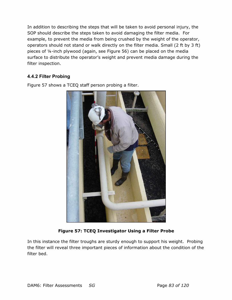
DAM6: Filter Assessments SG Page 83 of 120
In addition to describing the steps that will be taken to avoid personal injury, the SOP should describe the steps taken to avoid damaging the filter media. For example, to prevent the media from being crushed by the weight of the operator, operators should not stand or walk directly on the filter media. Small (2 ft by 3 ft) pieces of ¼-inch plywood (again, see Figure 56) can be placed on the media surface to distribute the operator’s weight and prevent media damage during the filter inspection.
4.4.2 Filter Probing
Figure 57 shows a TCEQ staff person probing a filter.
Figure 57: TCEQ Investigator Using a Filter Probe
In this instance the filter troughs are sturdy enough to support his weight. Probing the filter will reveal three important pieces of information about the condition of the filter bed.

DAM6: Filter Assessments SG Page 84 of 120
Specifically, the probing will allow the operator to:
• Measure the variations in the surface of the media support structure by measuring the distance from the top of the support layer to a fixed reference point, such as the top of the filter trough,
• Measure variations in the surface elevation of the media bed by measuring the distance from the reference point to the top of the media bed, and
• Measure variations in the media bed thickness by measuring the distance from the top of the support layer to the top of the media bed.
The entire surface of the media should be probed every 18 – 24 inches and, in order to avoid missing problems, intervals of more than 36 inches should be avoided. Too, the distance between measurements may need to be decreased substantially to precisely characterize the bed elevations and thicknesses in the vicinity of any backwash jets and media mounds and depressions.
Figure 58 shows a sample filter probing and excavation plan used by the TCEQ during a mCPE for a 7-foot by 12-foot filter.
Figure 58: Filter Probe Plan for a Small, 1-Trough Filter
In this example, the probe locations are about 2 feet apart in both directions. Of course, it is not practical to probe directly beneath the filter trough.

DAM6: Filter Assessments SG Page 85 of 120
While it is unusual for the surface of the media bed to vary more than an inch or two in a well-operated, well-maintained filter, it is not that unusual to find 2-inch to 3-inch variations in the surface elevation of the support system if the media rests on a gravel support. Variations of more than 1-inch are very unusual in a gravelless system. The thickness of the media bed can vary by 2 – 3 inches if gravel support is used and by 1 – 2 inches in a gravelless filter.
Figure 59 shows the measurements that will be noted during a filter probe.
Figure 59: Collecting Filter Probe Data
In Figure 59:
• The A measurement, from the top of the filter trough to the top of the support gravel, is recorded.
• The C measurement, from the top of the media to the top of the support gravel, is recorded.
• Then the B measurement, from the top of the trough to the top of the media is calculated from the previous two measurements.
Once the probe measurements are recorded and/or calculated, the measurements are used to determine the locations where the media bed is the thickest and thinnest, and where the support gravel is the highest and lowest. These locations are commonly selected for conducting media excavations to further evaluate the condition of the media bed. Other calculations commonly performed are the average media thickness and the average depth of the gravel.

DAM6: Filter Assessments SG Page 86 of 120
Figure 60 shows a representation of the some of the probe data collected during a mCPE.
Figure 60: Bed Uniformity and Thickness
The bar on the left represents the design specifications for the filter and reflects 12 inches of gravel supporting 29 inches of filter media (20 inches of anthracite and 9 inches of sand). The three bars on the right represent three filter probe locations. The data shows that the filter media was less than the design specification at every location. They also show that at two locations, the gravel had been mounded and at one location gravel had been displaced.
DAM6: Filter Assessments SG Page 87 of 120
These findings show that there had been a severe disruption of the gravel support and excessive loss of media. The media loss had actually been much more severe than indicated during the filter assessment, because the system engineer reported capping the filter with 6 inches of anthracite 10 days before the mCPE began.
As the chart in Figure 60 indicates, the gravel support layer in this filter was severely disrupted. Although it is possible that the gravel was not properly installed, the greater likelihood is that the filter has been damaged by careless backwashing or by air getting trapped in the filter effluent and/or backwash lines and then being evacuated through the filter when the backwash pump is turned on. Any sudden release of air through an underdrain that is not designed for air scour can cause damage. Localized air jets can form, dislodge gravel, and disrupt the media support layer.
In Figure 60, the average media depth was 26.5 inches, only 10% less than that described by the specification, the engineer for the plant stated that about six inches of anthracite was added to the filter 10 days before the mCPE. Therefore, until recently, the filter bed had about 30% less media than the specifications required. Further, the large disruptions in the gravel bed resulted in media depth and gravel depth variations that are more than three times greater than the 2 – 3 inch variation typically observed during filter inspections. The 11-inch difference between the filter bed design and the lowest point in the filter, as shown in Figure 60, was detectable without conducting filter probes, but the probing assisted in further defining the extent of the problem.
4.4.4 Media Excavations
Although probing the filter provides a lot of information about the depth and levelness of the filter bed and its support system, it does not provide any insight into what is happening within the filter bed. To gain this information, the media bed needs to be excavated at one or more locations.
It is particularly important to excavate sites where mounds or depressions were seen when the filter was drained, backwash water jets have been observed, and filter probe measurements detected gravel mounds. During the excavation, the operator will be able to verify probe measurements, look for subsurface mudballs, determine if the different media layers are properly stratified, and evaluate the condition of the media grains to decide if other special studies are needed.
Figure 61 shows a Comprehensive Performance Evaluation Team performing an excavation during a filter assessment.
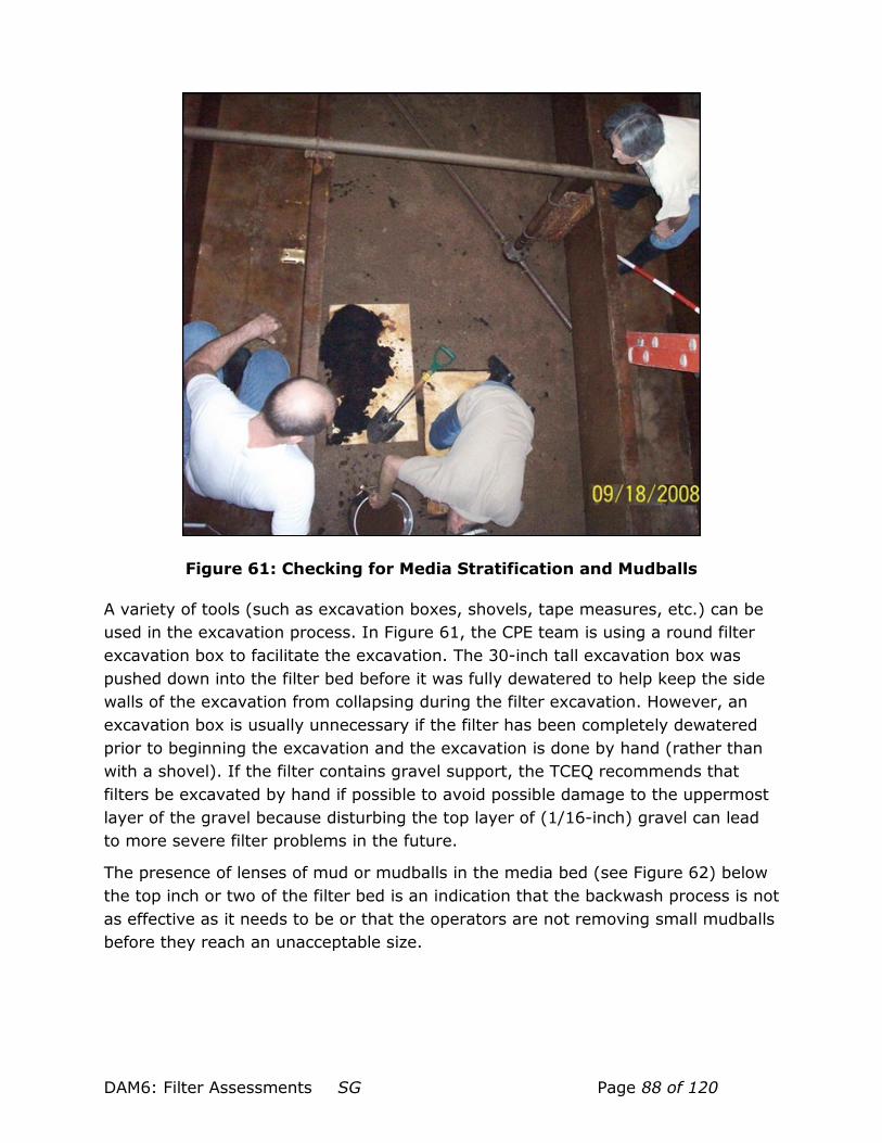
DAM6: Filter Assessments SG Page 88 of 120
Figure 61: Checking for Media Stratification and Mudballs
A variety of tools (such as excavation boxes, shovels, tape measures, etc.) can be used in the excavation process. In Figure 61, the CPE team is using a round filter excavation box to facilitate the excavation. The 30-inch tall excavation box was pushed down into the filter bed before it was fully dewatered to help keep the side walls of the excavation from collapsing during the filter excavation. However, an excavation box is usually unnecessary if the filter has been completely dewatered prior to beginning the excavation and the excavation is done by hand (rather than with a shovel). If the filter contains gravel support, the TCEQ recommends that filters be excavated by hand if possible to avoid possible damage to the uppermost layer of the gravel because disturbing the top layer of (1/16-inch) gravel can lead to more severe filter problems in the future.
The presence of lenses of mud or mudballs in the media bed (see Figure 62) below the top inch or two of the filter bed is an indication that the backwash process is not as effective as it needs to be or that the operators are not removing small mudballs before they reach an unacceptable size.

DAM6: Filter Assessments SG Page 89 of 120
Figure 62: Mud in the Media Bed
If the filter contains more than one type of media (e.g. anthracite over sand), a certain degree of intermixing is inevitable. However, if the thickness of the intermixed layer exceeds 2 – 3 inches, the operators need to make sure that they are ramping down the backwash water flow rate slowly enough to allow proper stratification of the media layers.
Figure 63 shows a media excavation where small pockets of sand are present in the anthracite layer and a pocket of anthracite is located in the sand layer.
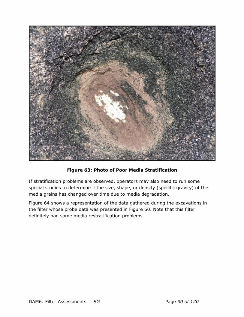
DAM6: Filter Assessments SG Page 90 of 120
Figure 63: Photo of Poor Media Stratification
If stratification problems are observed, operators may also need to run some special studies to determine if the size, shape, or density (specific gravity) of the media grains has changed over time due to media degradation.
Figure 64 shows a representation of the data gathered during the excavations in the filter whose probe data was presented in Figure 60. Note that this filter definitely had some media restratification problems.

DAM6: Filter Assessments SG Page 91 of 120
Figure 64: Poor Media Stratification
Following the filter probe, a mCPE team member entered the drained filter to evaluate the surface and subsurface condition of the filter bed. In Figure 64, the first excavation was conducted at a site where a media mound was observed, the second at a depression site where the probe detected a shallow media depth and a gravel mound, and the third at a site where the bed depth (or thickness) was more consistent with the original specifications (which is shown in the last column).
The excavations revealed that there was a layer of floc on top of the filter approximately 1/16-inch thick. Although there were smaller mudballs located throughout the surface of the filter bed, some areas of the filter contained mudballs as large as 2-inches wide by 3-inches long by ¼-inch thick on top of the filter media.

DAM6: Filter Assessments SG Page 92 of 120
The presence of the thin, uniform floc layer was consistent with conditions normally found in filters that have been in service for several hours. However, mudballs are clumps of floc particles that form over the course of many filter runs. The presence of mudballs, especially large mudballs, suggests that the filter is not being adequately cleaned during the backwash process and that the operators are not removing mudballs as they form. After completing the surface inspection, the team excavated the filter bed at three sites to inspect the subsurface condition of the media bed.
The excavations revealed that the media grains were clean, angular, sharp, and in otherwise good condition. No mudballs were observed below the surface of the media and so the team concluded that the backwash process was preventing a significant subsurface migration of mudballs even though it was not preventing them from forming on the surface of the filter bed. However, the inconsistent composition of the media layers (i.e., the thickness of the media layers and their interfaces) suggests that the irregular thickness of the gravel layer is producing undesirable, uneven distribution of backwash water. This finding was supported by the presence of gravel in the sand layer of the filter bed.
Finally, the excavations revealed that there has been some intermixing of the gravel, sand, and anthracite layers in the filter. At two of the sites, the 3-inch thick transition zone between sand and anthracite is consistent with the 2 or 3-inch interface found in well-operated filters. However, at the first site, there was a 4-inch interface between sand and anthracite and the bottom 6 inches of sand contained increasing amounts of fine gravel.
4.5 Backwash Rise Rate and Bed Expansion In technical terms, the rise rate is the upward velocity of water at the peak backwash rate. For most of us, it is how fast the water level rises when the backwash pump is at the highest level, and the backwash to waste line is closed off. Bed expansion is normally described by the percentage that the depth of the filter bed increases at the peak backwash rate.
4.5.1 Rise Rate
During the backwash, the upward flow of water agitates and expands the media bed and removes floc from the pores and surface of the media grains. Figure 65 shows the procedure for confirming the backwash rise rate in the filter.

DAM6: Filter Assessments SG Page 93 of 120
Figure 65: Calculating Rise Rate
At higher rise rates, larger floc particles can be lifted out of the expanded bed so higher rise rates are better than low rise rates. In addition, higher rise rates are generally required if the filter does not have a supplemental air scour system than if it does because the air scour process turns tends to turn large floc particles into small floc particles that are easier to remove.
On the other hand, if the rise rate gets too high, the upward velocity can expand the bed so much that the media can reach the backwash trough and get flushed from the filter along with the floc particles. Therefore, the maximum permissible rise rate depends on type of media used in the filter (i.e., media size and density) and the distance from the top of the unexpanded bed to the top of the backwash trough (i.e., the filter freeboard). To a certain extent, the maximum allowable rise rate is also affected by water temperature because the viscosity and density of the water changes as the temperature changes. At colder temperatures, the water becomes more dense and viscous and so the rise rate may need to be lowered slightly to prevent media loss.
For most filters, rise rates that are between 20 inches of vertical rise per minute (a peak backwash rate of 12.5 gpm/ft2) and 35 inches per minute (a peak backwash

DAM6: Filter Assessments SG Page 94 of 120
rate of about 22 gpm/ft2) should provide adequate cleaning without excessive media loss. Monomedia beds of granular activated carbon (which has a lower density that most other media) can be backwashed on the lower end of the scale while monomedia beds of sand (which has a relatively high density) will often need to backwashed on the upper end of the range.
Figure 65 shows the procedure for confirming the backwash rise rate in the filter. The rise rate determination using a hook gauge is similar to the procedure for confirming the function of the backwash flow meter.
4.5.2 Bed Expansion
To determine the bed expansion, the operator must know the bed depth before the backwash cycle and the amount that the depth increased when the bed was expanded. Figure 66 shows how bed expansion is calculated from measurements taken in the filter.
Figure 66: Calculating Bed Expansion

DAM6: Filter Assessments SG Page 95 of 120
As shown in Figure 66, to obtain these two pieces of information, the operator must measure:
• the distance (A) from the top of the unexpanded bed to a reference point in the filter (usually the top of the filter box) before beginning the backwash cycle, and
• the distance (B) from the top of the expanded bed to the reference point in the filter at the peak backwash water flow rate, and the depth (C) of the unexpanded media bed before beginning the backwash cycle.
For facilities equipped with air scour, bed expansions of 10 – 15% are generally adequate because the air scour process does a very good job of turning large floc particles into small floc particles which are easier to remove. For mixed-media filters without air scour, bed expansions of 15 – 25% are sometimes needed to adequately clean the filter. For mono-media sand filters without air scour, expansions of 20 – 40% may be necessary.
Figure 67 shows two different types of bed expansion measurement devices.
Figure 67: Bed Expansion Measurement Tools

DAM6: Filter Assessments SG Page 96 of 120
The device in the top of the photo is assembled and used to measure from the top of the filter wall (or backwash trough) to the surface of the filter bed (the A reference measurement). Then at the maximum backwash flow rate, the operator lowers the device until filter media just begins to collect on the partial plate. At this point the “B” measurement is recorded. (Figure 68 shows two engineers performing this task.)
Figure 68: Two Engineers Measure Bed Expansion
The “C” reference measurement is taken by probing or by some other direct measurement. Once all the measurements are assembled, the calculation shown in Figure 66 is performed.
As the backwash water flow rate is incrementally increased during the backwash cycle, the upward velocity increases and the resulting forces cause the filter grains begin to shake. At some point, called the incipient fluidization velocity, the grains on the top of the filter will begin being pushed up out of the bed which lowers the pressure on the particles beneath them and they, too, begin to rise.
Any additional increase in the backwash water flow rate will cause the bed to begin expanding. Once the backwash water reaches its maximum upward velocity (i.e., the maximum backwash rate), the bed will expand no further.
It is important to understand that bed expansion is not uniform throughout the entire depth of the filter bed. In addition to the fact that the anthracite is lighter and more easily lofted that the sand beneath it, the grains at the top of the filter

DAM6: Filter Assessments SG Page 97 of 120
will rise further than the grains at the bottom of the filter because there is nothing to hold them down.
However, the upward movement of the grains at the bottom of the filter is restricted because there are grains above them that are in the way and because these upper grains are trying to fall back down into the filter. Therefore, bed expansion in the upper portion of the bed will be greater than bed expansion in the lower portion of the bed. This is important because it means that it is difficult to get a mudball out of the filter bed once it has made its way down into the lower portion of the filter.
4.5 Media Condition There are a variety of special studies that can be conducted to evaluate the condition of the media. However, these tests are usually considered to be optional unless the filter excavations suggest that there might be a problem with the media or if the operators cannot otherwise explain anomalies noted during data reviews or routine observations. A relatively complete evaluation of the media condition involves conducting several tests:
• sieve analysis to determine the size of the media grains and the L/d ratio of the filter bed,
• density analysis to determine the specific gravity of the media grains,
• microscopic inspection to evaluate the appearance of the media grains,
• solubility tests to determine the degree to which material has been deposited on the surface of the media,
• mudball retention analysis to evaluate the effectiveness of filter backwash, and
• floc retention analysis.
4.5.1 Sieve Analysis8
4.5.1.1 Why Media Size is Important
As noted previously, the size and shape of media grains can change over time. Friable (fragile) materials, such as granular activated carbon grains, can get crushed by the weight of the media above them and the grains of relatively soft materials, like GAC and anthracite, tend to get worn down as they bump together
8 The procedure outlined here is a field test and no attempt was made to conform precisely to the ASTM C136-04 procedure for conducting granular media sieve analyses.
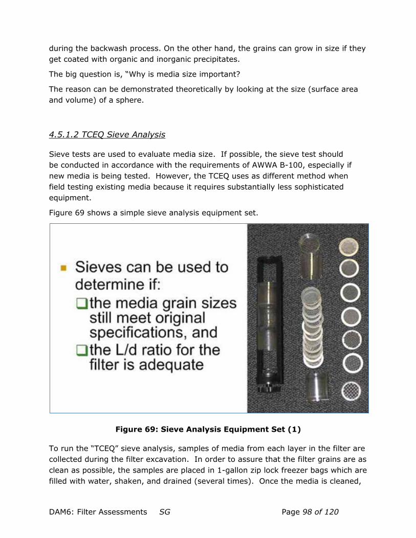
DAM6: Filter Assessments SG Page 98 of 120
during the backwash process. On the other hand, the grains can grow in size if they get coated with organic and inorganic precipitates.
The big question is, “Why is media size important?
The reason can be demonstrated theoretically by looking at the size (surface area and volume) of a sphere.
4.5.1.2 TCEQ Sieve Analysis
Sieve tests are used to evaluate media size. If possible, the sieve test should be conducted in accordance with the requirements of AWWA B-100, especially if new media is being tested. However, the TCEQ uses as different method when field testing existing media because it requires substantially less sophisticated equipment.
Figure 69 shows a simple sieve analysis equipment set.
Figure 69: Sieve Analysis Equipment Set (1)
To run the “TCEQ” sieve analysis, samples of media from each layer in the filter are collected during the filter excavation. In order to assure that the filter grains are as clean as possible, the samples are placed in 1-gallon zip lock freezer bags which are filled with water, shaken, and drained (several times). Once the media is cleaned,

DAM6: Filter Assessments SG Page 99 of 120
it must be dried before it can be sieved. (TCEQ staff have been known to simply spread the media sample out on several sheets of newspaper to absorb the water.)
While the sample is drying, a set of weighing dishes (or, in the TCEQ’s world of field work, disposable plastic cups) are weighed on a scale that has a precision of no less than 0.01 grams. In addition, the sieving apparatus is assembled with the largest-sized sieve that is expected to capture any media on (the bottom of) the top chamber and the progressively smaller sieves on the lower chambers. The bottom chamber has a solid bottom and collects all of the grains that pass through all the sieves (which are itself re-sieved using progressively smaller sieve sizes until the bottom chamber contains essentially no media).
The top chamber is then filled 2/3rd full of media from the dried sample and gently (or sometimes not so gently) shaken until the sample is fully sieved (usually about 8 – 10 minutes). The samples captured in each chamber are then placed in separate pre-weighed plastic cups and weighed. The net weight of the sample in each chamber is recorded and the total weight of the samples is calculated.
Figure 70 shows a picture of the TCEQ equipment during use.
Figure 70: Sieve Analysis Equipment (2)

DAM6: Filter Assessments SG Page 100 of 120
The sieve size information and weight of each sample is then entered in a spreadsheet which the TCEQ staff developed to calculate the percentage of media passing though each sieve (see Figure 71). The effective size, or d10, of the media is the size of the sieve that allows 10% of the media (by weight) to pass. The uniformity coefficient of the media is the size of the sieve that allows 60% of the media (by weight) to pass divided by the size of the sieve that allows 10% of the media (by weight) to pass.
Figure 71: Sieve Table: Effective Size and Uniformity Coefficient Calculator
4.5.1.3 ES and UC Chart
Since it is not practical to expect exactly 10% (or 60%) of the media to be retained on a sieve screen, the spreadsheet displays the “percent passing” data on a chart where the 10% and 60% values of each media layer is read where these percent lines cross the media size graph. The d10 and d60 values are read off the X-axis. (see Figure 72).
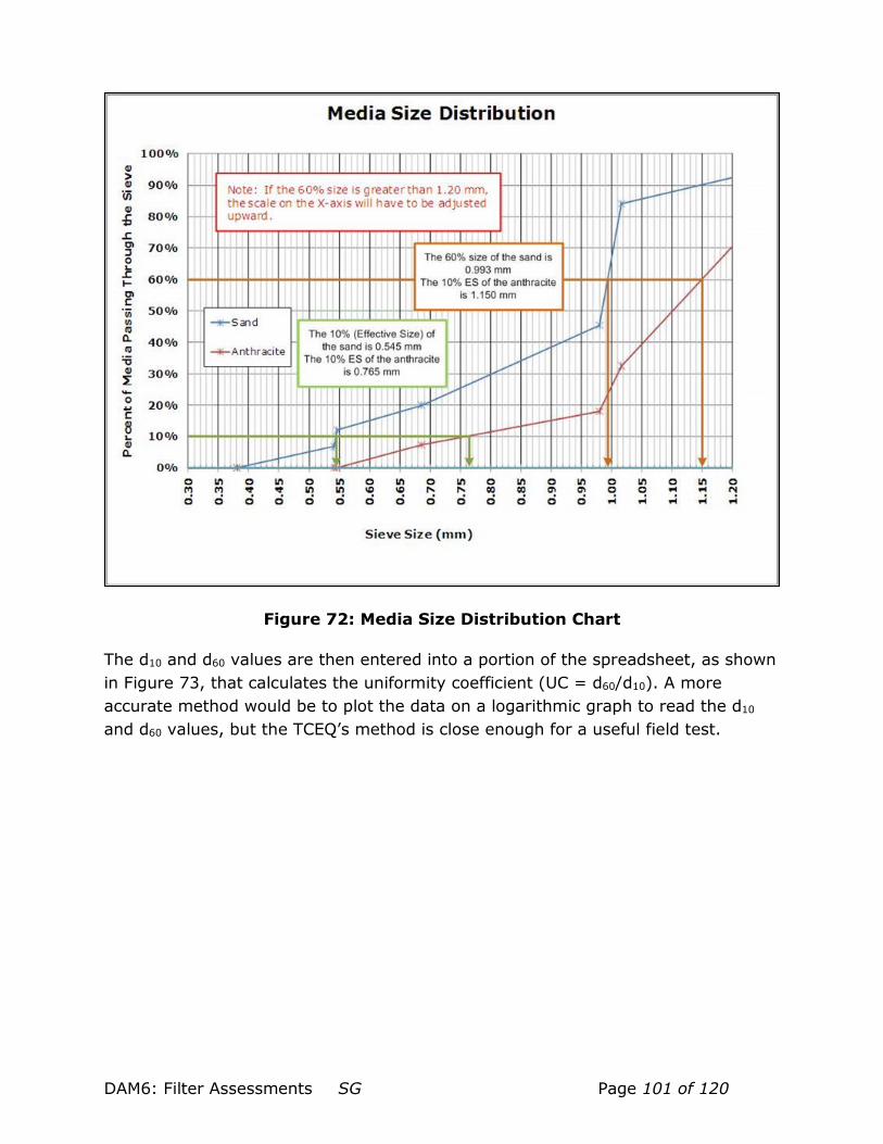
DAM6: Filter Assessments SG Page 101 of 120
Figure 72: Media Size Distribution Chart
The d10 and d60 values are then entered into a portion of the spreadsheet, as shown in Figure 73, that calculates the uniformity coefficient (UC = d60/d10). A more accurate method would be to plot the data on a logarithmic graph to read the d10 and d60 values, but the TCEQ’s method is close enough for a useful field test.

DAM6: Filter Assessments SG Page 102 of 120
Figure 73: Uniformity Coefficient Table
The L/d ratio for a media bed is the bed thickness (or Length of the bed) divided by the effective size (or diameter) of the media. Figure 74 shows how this ratio is calculated using a spreadsheet.

DAM6: Filter Assessments SG Page 103 of 120
Figure 74: L/d Ratio Calculations
In dual-media and multi-media beds, the L/d ratio is the sum of the L/d ratios for the individual layers in the bed. The TCEQ measures thickness (Length) in inches but effective size (diameter) in millimeters. Consequently, their spreadsheet includes an L/d calculator so that they don’t have to remember that there are 25.4 mm per inch.
L/d is an important parameter because it provides a way to compare the performance of different filter bed designs.
In general, filters with an overall L/d that is greater than 1000 are capable of producing high-quality water throughout the filter run at a 95% or better efficiency. Although filters with lower L/d ratios will work, they often have a more difficult time producing high-quality water in the first few hours of the filter run and are more susceptible to filter spikes (because they have fewer filter grains and, therefore, less surface area to capture particles).
Filters with lower L/d ratios may also more likely to have shorter filter runs because there are fewer pores in the filter bed to hold the floc at the end of the run.
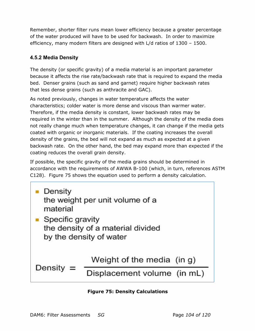
DAM6: Filter Assessments SG Page 104 of 120
Remember, shorter filter runs mean lower efficiency because a greater percentage of the water produced will have to be used for backwash. In order to maximize efficiency, many modern filters are designed with L/d ratios of 1300 – 1500.
4.5.2 Media Density
The density (or specific gravity) of a media material is an important parameter because it affects the rise rate/backwash rate that is required to expand the media bed. Denser grains (such as sand and garnet) require higher backwash rates that less dense grains (such as anthracite and GAC).
As noted previously, changes in water temperature affects the water characteristics; colder water is more dense and viscous than warmer water. Therefore, if the media density is constant, lower backwash rates may be required in the winter than in the summer. Although the density of the media does not really change much when temperature changes, it can change if the media gets coated with organic or inorganic materials. If the coating increases the overall density of the grains, the bed will not expand as much as expected at a given backwash rate. On the other hand, the bed may expand more than expected if the coating reduces the overall grain density.
If possible, the specific gravity of the media grains should be determined in accordance with the requirements of AWWA B-100 (which, in turn, references ASTM C128). Figure 75 shows the equation used to perform a density calculation.
Figure 75: Density Calculations
DAM6: Filter Assessments SG Page 105 of 120
A “field test” procedure (which does not conform to the either standard) for assembling the data for the density calculation is as follows:
• Place 20 mL of room-temperature water in a 50 mL graduated cylinder
• Weigh out 25 – 30 grams of the (cleaned and dried) media sample used for the sieve analysis to the nearest 0.1 gram.
• Slowly add the media sample to the graduated cylinder
• Agitate the cylinder to dislodge any air bubbles that might have attached to the grains as they were added to the cylinder
• Measure the increase in the water level to the nearest 1 mL (or, if possible, the nearest 0.5 mL).
• NOTES: if the water level rises above the 50 mL mark, repeat the test with slightly less water.
Divide the weight of the sample by the increase in water volume to determine its density (in g/mL).
The principle problem with this field method is that the 50 mL graduated cylinders are usually marked in 1 mL increments. Therefore, the accuracy of the density measurements can be no better than +/- 2% and will likely be no worse than +/- 5% (although a 10% error is theoretically possible if the starting volume is under-reported by 1 mL and final volume is over-reported by 1 mL and the density of the filter grain is 1.0). Still, that’s pretty good for field work.
4.5.3 Microscopic Inspection
Microscopic inspections can be conducted using a dissection microscope or a digital camera with a macro capability. The TCEQ staff have had great results using a variety of digital cameras including a 10-megapixel compact camera, an 8-megapixel full-body consumer camera, and a digital SLR.
Examples of good and poor media quality are shown in Figure 76.

DAM6: Filter Assessments SG Page 106 of 120
Figure 76: Microscopic Examination of Good and Poor Media
As shown in Figure 76, good media will normally:
• be irregularly shaped
• have sharp edges
• be free of incrustations.
On the other hand, poor quality media may be characterized by:
• rounded shape and edges,
• broken media grains, and
• encrustations of calcium carbonate or other materials.
DAM6: Filter Assessments SG Page 107 of 120
4.5.4 Solubility Tests9
Solubility tests are generally warranted only if new media is being installed or if visual observations, media probes, or other special studies indicate that the existing media grains may be encrusted. If there are problems, solubility tests allow the operator to calculate the degree of encrustation as well as to give some indication as to what material may be coating the grain.
Solubility tests on new media should be conducted in accordance with the requirements of AWWA B-100 (which specifies a 110oC drying temperature and a desiccator).
However, the TCEQ Optimization Program staff have found the following alternative method to be useful when evaluating the condition of existing media.
• Rinse, dry, and weigh a 50+ gram sample of media to an accuracy of 0.1 grams
• Place sample in a 300 – 400 mL of an acidic or basic solvent (e.g. 50% HCl)
• During the first 10 minutes, observe the sample to see if bubbles are forming or the sample is effervescing
• After 10 minutes, stir or mix the sample periodically for 30 – 60 minutes. (Actually, this step continues for at least 30 minutes after the bubbles stop forming, even if that takes an hour.)
• If the solvent is going to be submitted for chemical analysis, transfer it in to the sample container that will be submitted to the lab.
• Rinse, dry, and reweigh the media sample.
Although the principal purpose of running a solubility tests is to gather the data needed to calculate the % Solubility of the media, the test can also provide the operator some basic information about what material might be coating the filter grains.
For example, if the media begins to bubble when immersed in an acidic solvent, the encrustation probably contains a significant amount of calcium carbonate. If an acidic solvent gradually turns yellow or light brown over the course of the test, the coating likely contains some iron but if it turns grey or black, it probably contains some manganese.
9 The procedure outlined in this subsection is a field test and no attempt is made to conform precisely to the AWWA B100-01 procedure which is used to confirm the acid solubility of media.

DAM6: Filter Assessments SG Page 108 of 120
Figure 77 shows a media sample encrusted with iron and manganese. Notice that the iron dissolved first, and then the manganese.
Figure 77: Solvent Appearance During Media Grain Acidification
Most inorganic encrustations are more soluble in acidic solvents. However, one of the TCEQ’s Optimization Program staff has found that algal coatings seem to be more soluble in basic solvents than in acidic ones.
Figure 78 shows examples of sand and anthracite before and after acidification.
Figure 78: Appearance of Media Before and After Acidification
The left side of Figure 78 shows the change in media volume that resulted when a dilute acid was added to one of two equal sand media samples to dissolve the apparent manganese deposits. The figure clearly shows why the operators had noticed that the volume of their filter bed had increased over time. The figure also

DAM6: Filter Assessments SG Page 109 of 120
illustrates that the coating had changed the specific gravity of both the anthracite and the sand to the point where the two media had begun to intermix because the specific gravities has become more similar. Weighing the two media samples indicated that the test removed about 20.5% of the original mass. The acid solubility is significantly greater than the 5% solubility allowed for new media.
The right side of Figure 78 shows the change in media volume that resulted when a dilute acid was added to one of two equal anthracite media samples to dissolve the apparent calcium carbonate deposits. The upper photo shows the encrustations that had developed on the anthracite and the lower photo reveals the condition of the anthracite grains after the deposits had been removed. Although it may be difficult to see, the clean anthracite was in fairly good condition, was irregularly-shaped, and had reasonably sharp edges.
Figure 79 shows the change in media volume that resulted when one of two equal media samples was treated with a dilute acid and then a dilute base.
Figure 79: Media Grain Volume and Appearance Before and After Acid/Base Cleaning

DAM6: Filter Assessments SG Page 110 of 120
Although we have no photo of the sample in Figure 79 after acidification and before treating with the dilute base, the acid treatment did not have much effect on the volume of the media sample. However, the coating (which appeared to be algal in nature) was removed by the dilute base. Weighing the two media samples indicated that the test removed about 18.1% of the original mass. Although there is no standard for base solubility, the photo clearly shows why the operators had noticed that the volume of their filter bed had increased dramatically over the 20+ years that the sand had been in the mono-media filter.
The two photos on the right side of Figure 79 show a few grains that were removed from the two samples. The upper photo shows the algal coating on the sand grains and the lower photo reveals the condition of the sand grains after the deposits had been removed. Although it may be difficult to see, the clean sand is not in pristine condition; although silica sand grains do tend to be more spherical that anthracite or GAC grains, these grains lack the rough surface that is typically seen in new sand media.
The equation shown in Figure 80 is used to calculate the percent solubility of used media.
Figure 80: Calculating Percent Solubility
One should be aware that there is no solubility standard for used media, but the calculation does provide a measure for how much encrustation has occurred. AWWA B100-01 specifies that the acid solubility limits of new silica sand, anthracite, and high density sands (i.e., garnet, ilmenite) shall be less than 5%. Encrusted media will have solubility greater than 5%.
The table in Figure 81 shows the original, in-situ, and post-acidification specifications for the media shown in Figure 79.

DAM6: Filter Assessments SG Page 111 of 120
Figure 81: Comparison of Media Specifications – Before and After Acidification
Note that the anthracite was not acidified, as it had been installed only a week before this analysis was performed. It can be seen by the change in size and uniformity coefficient for the sand, that encrustation had made the sand larger.
Good engineering practice and TCEQ regulations specify that the L/d ratio for a media bed (a measure of the bed’s thickness to the effective size of the media grains) should be at or greater than 1,000.
An example of an L/d calculation for a media bed is shown in Figure 82.

DAM6: Filter Assessments SG Page 112 of 120
Figure 82: L/d Ratio Calculation for a Media Bed
In this example, Media 1 (sand) has a thickness of 16” (406.4 mm) and Media 2 (anthracite) has a thickness of 29” (736.6 mm). The specified effective sizes of the two media are 0.69 mm and 1.22 mm, respectively. By summing the L/d ratio for the individual media layers, the total L/D ration is calculated to be 1193.
Figure 83 shows the L/d calculations for the “in situ” media shown in Figure 79 and described in Figure 81.

DAM6: Filter Assessments SG Page 113 of 120
Figure 83: L/d Ratio Calculation for an Old Media Bed
The engineering drawings for the plant indicated that the filters were designed to contain 12 inches of 0.45 mm sand and 15 inches of 0.68 mm anthracite. Based on these specifications, the filter bed was designed to have an L/d ratio of 1,242. Based on the actual depth and effective sizes (23 inches of 0.55 mm sand and 7 inches of 0.69 mm anthracite) found during the mCPE, the L/d ratio for the filter bed is 1,320. Based on this number, one could hastily assume that the filter should be working better than designed, however, it was not. The L/d ratio is an effective tool only as long as other design parameters are also in effect. As noted previously, this particular filter performed poorly enough to trigger the mCPE. Although the L/d ratio for the existing filter met minimum TCEQ requirements, filter performance was severely degraded.
Anthracite grains are typically much larger than sand grains. Therefore, the spaces (or pores) between anthracite grains are larger than the pores between the sand grains. Although larger pore sizes increase the amount of floc that can be held before breakthrough occurs, larger pores allow more floc to pass during the initial stage of the filter run. To compensate for this performance characteristic, the TCEQ recommends that dual media filter contain a thick layer of anthracite. Dual-media filters typically contain at least 24 inches of 0.9 – 1.0 mm anthracite to maximize the performance of this layer.
Because sand grains are smaller than anthracite grains, the pore sizes are smaller. Assuming the sand is in good condition, the small pores between the sand grains will trap the floc particles that escape from the anthracite at the beginning of the filter run. However, the small pores in the sand will fill with floc faster than the large pores in the anthracite. Consequently, if there is not enough anthracite, the sand layer accumulates floc very quickly and the time that elapses before particles

DAM6: Filter Assessments SG Page 114 of 120
begin to break through the filter is greatly reduced. Since the pore sizes are fairly uniform throughout the sand layer, most of the floc that escapes the anthracite layer is trapped in the top 6 – 12 inches of the sand. For this reason, significantly increasing the thickness of the sand layer of this same size does not necessarily improve filter performance. Based on the performance characteristics of sand, the TCEQ recommends that the sand layer in a dual media filter contain 12 inches or so of 0.45 – 0.55 mm sand.
Without an adequate layer of properly sized anthracite, the top portion of the sand layer experiences surface binding earlier than would be experienced if there were enough anthracite to capture more of the larger floc particles in the depths of the anthracite layer rather than near the top. Having more sand, less anthracite, and smaller anthracite greatly reduced the time the filter run before particle breakthrough. In fact, the operators at this plant were backwashing their filters at least once per day, and sometimes twice per day due to rising turbidity levels.
4.5.5 Mudball Content
As noted previously, mudballs should be removed if they cover more than 5% of the bed surface, become larger than ½-inch in diameter, or more than ¼-inch thick. However, that “visual” approach only evaluates the mudball concentration on the surface of the media. To evaluate the mudball content of the entire bed, a percent mudball test must be run. Nevertheless, the percent mudball test does not provide much more information than a cursory surface inspection unless a filter excavation has revealed that mudballs have formed in (or migrated down into) the filter bed.
If the excavation does reveal a significant number of subsurface mudballs, operators can use the following procedure to quantify the overall mudball content of the entire bed:
• Backwash the filter to remove any accumulated floc
• Drain the filter and use a 3 – 6-inch coring tool to collect a representative sample of media from the entire depth of the bed, or use a 2-inch coring tool to collect three or four representative samples from the filter.
• Measure the total volume of the core by slowly placing portions of the sample in a 2-liter graduated cylinder that contains 300 mL of water and recording the increase in water level. (Repeat this measurement as many times as necessary until the all of the core has been evaluated. Make sure that 30 – 40 mL of water remains above the added media so that accurate measurements can be made of the increase in volume. If necessary, invert or gently shake the cylinder to release any air bubbles that might have attached to the media grains when they were added.)

DAM6: Filter Assessments SG Page 115 of 120
• After each measurement, pour the contents of the cylinder though a through a 4-mesh hardware cloth to collect mudballs. GENTLY shake the hardware cloth to screen out the mudballs.
• Add the individual results of each measurement to get the total volume of the media core.
• After screening all of the samples, measure the volume of the mudballs by slowing adding them to in a 1-liter graduated cylinder that contains 300 mL of water and recording the increase in the water level.
• Calculate the percent mudball content by dividing the total volume of the core sample by the volume of the mudballs and multiplying by 100.
Figure 84 shows the two pieces of a mudball from a poorly maintained filter.
Figure 84: Mudballs from a Poorly Maintained Filter
In this example, the mudball was several inches thick and more than 3 feet in diameter. These small pieces were all that could be pried loose from the very compacted surface of the mudball.
Various sources characterize the relationship between mudball content and filter media condition in slightly different ways. However, the general consensus seems to be that a filter than contains less than 0.5% mudballs is in acceptable condition and those filter beds containing more than 5% mudballs are in terrible condition.
A generalization of the guidelines from these various references in presented in Figure 85.

DAM6: Filter Assessments SG Page 116 of 120
Figure 85: Mudball Content Analysis
4.5.6 Floc Retention Analysis
As discussed earlier, current design practices are focused on the principle that floc and other particles are captured by the media, throughout the depth of the media bed. A floc retention analysis is a method of determining whether or not this is happening. Some references discussing this analysis address statistical methods used to ensure the statistical validity of the test. As discussed here, however, a floc retention analysis is a “field test” used to determine, on a relative basis, the percentage of particles which are being collected at different levels in the filter.
• Take the filter off-line before backwashing and drain the filter.
• Core the bed to obtain media samples from the full depth.
o If a coring tool is not available, the media sample may be excavated with a trowel.
o Care must be taken not to disturb the gravel support layer and/or plastic nozzles if present.
• Categorize the samples based on the filter depth location.
o If samples are collected from more than one location across the media surface, these samples may be combined, but if so, they must be well mixed prior to step 4.
• Place 100 mL of media from the first sample into a 250 mL graduated cylinder with a stopper top.
• Fill the cylinder to the 200 mL mark (tap water is okay for this test).

DAM6: Filter Assessments SG Page 117 of 120
• Shake by oscillating the cylinder sideways with a swing of at least 8 inches for at least one minute.
• Stand the cylinder on a level surface long enough for the media to settle. If the level is below the 100 mL mark, add small amounts of media from the same sample till the media reaches the 100 mL.
• Shake the sample again, for a few seconds, and then top off the cylinder to the 250 mL mark.
• Shake the cylinder again for at least one minute.
• Let the media settle and decant a small sample into a turbidimeter sample tube.
• Take the turbidity reading of decanted water
• Repeat steps 4 through 11 for all the remaining samples from the different levels within the filter bed.
• Repeat entire process after backwashing filter
As noted previously, there are slight variations in the techniques that various sources use to characterize the relationship between mudball content and filter media condition. A similar situation seems to exist for evaluation of floc retention analysis data.
Figure 86 is a fair summary of the different guidelines. 10
Figure 86: Floc Retention Analysis Guidelines
10 The TCEQ’s Optimization Program staff have never done a floc retention analysis. Therefore, the table presented in this slide is a composite of the guidelines contained in a variety of literature.

DAM6: Filter Assessments SG Page 118 of 120
The consensus seems to be that it is not good to get the filter too clean and it is not good to leave the filter too dirty. Getting a filter too clean increases the ripening time and leaving it too dirty can produce severe post-backwash turbidity spikes, shorten the filter run, and contribute to mudball formation.
Figure 87 shows the before backwash and after backwash samples for a mono-media filter bed and a dual-media bed taken from USEPA literature.
Figure 87: Floc Retention Analysis Charts
As discussed earlier, the surface of the media layer tends to collect the most particles, but in the mono-media filter, approximately the same amount of floc was deposited at each sample location from 1.5 feet below the surface to the bottom of the filter bed. This shows that the filter is in fact operating in a “depth filtration” mode, as designed. The chart for the dual-media bed shows the same characteristic in the top layer of media, but it also has a second high incidence of particle collection at the top of the sand/anthracite interface. This reflects the premise that the top section of a media layer will collect the most particles, but it can also be seen that below the interface, each sample, again collected approximately the same amount of floc.
If an operator chooses to not mix the pre-back-wash media samples from the different core locations, a map of where the floc is being deposited can be developed for each layer of media. Similarly, using the post-backwash media samples, the operator can develop a map of those locations where the backwash appears to be more or less effective. Finally, the literature states that this analysis

DAM6: Filter Assessments SG Page 119 of 120
can be used to compare the floc deposition in problem areas (i.e., where jetting, mounding, or where holes are formed) with the general characteristics of the more “normal” areas of the filter.

DAM6: Filter Assessments SG Page 120 of 120

DAM6: Filter Assessments
Staff Guidance A-1
Appendix A: Student Guide
Workshop 1: Why Optimize?
Format: Lecture
Time: Approximately 25 minutes.
Note: Time not taken during the lecture should be used for general discussion of the importance that surface water treatment has on public health.
Trainer: DAM6 trained instructor
Tools/equipment: Notes sheet:
Reduced Cost of Operation
When filters are performing optimally, costs of operation can go down. Savings may accrue from:
• filter runs,
• filter backwash volumes,
• useful life of the filter media, and/or
• filter maintenance costs.
Reduced Public Health Risk
The most important reason for the drinking water regulations and filters in drinking
water plants is that human health is at risk when in the source water are not removed.
For each raw water source, particle (turbidity) removal is correlated to
x removal, and many scientific studies confirm this.
Particle Removal at Different Phases of Stable Operation
• During the more stable parts of the filter cycle, the filter can achieve up to
DAM6: Filter Assessments
Staff Guidance A-2
-log (99.999 to 99.9999 percent) pathogen removal.
• Near the end of the parts of the filter cycle, a filter may achieve only
-log (99 to 99.9 percent) pathogen removal.
• At the filter breakthrough part of the cycle, a filter may achieve only
-log (97 to 99 percent) pathogen removal.
Particle Removal during Filter Ripening
Ninety percent of the particles passing through a filter pass during the filter
period following a backwash.
Therefore, the duration of the ripening period and reducing the
magnitude of the post-backwash turbidity/particle spike would reduce the number
of passing through a filter.
Improved Filter Value
Reducing the number of particles passing through a filter improves the “value” of the filter, in terms .

DAM6: Filter Assessments
Staff Guidance A-3
Workshop 2: Introduction to Trend Analysis Format: Demonstration and Practical Exercise
Time: Approximately 45 minutes.
Trainer: DAM6 trained instructor
Tools/equipment:
• A computer with Excel software, a color display, and a CD ROM drive or USB port
• A color printer
• An electronic cop of the Data File “WrkShop-2-Trends.xlsx”
In this workshop, the trainer will open and display the Workshop 2 spreadsheet, showing the SWMOR data from Pages 2 and 3 of the SWMOR. There will be no data entry in this workshop, but the operator may choose to use the Workshop 2 data file to enter current local information at a later time.
Workshop 2 - Step 1
Copy the DAM6 files to the local computer. Your trainer will copy the DAM6 Documents from the CD into a DAM6 to a directory the operators create for this DAM.
Workshop 2 - Step 2
The trainer will open the copied file and review the spreadsheet entitled “P.2-Turbidity Data.”
• The left hand portion of P.2 page is set up exactly like Page 2 of the SWMOR.
o Review the data on the left hand side of the page to draw conclusions about the fictional plant represented by this form. Specific pertinent facts include:
The plant was on-line all 31 days of the month.
The plant was on-line 24 hours each day for the entire month.
The plant has two sedimentation basins, but Basin 1 was off-line for several days.
The average daily raw water pumpage was about 1.1 MGD.

DAM6: Filter Assessments
Staff Guidance A-4
The maximum daily raw water pumpage was about 1.8 MGD, or more than 1.6 times the average daily pumpage.
The minimum daily raw water pumpage was about 0.6 MGD, or slightly more than half of the average daily pumpage.
o With trainer participation, consider and discuss the implications of these facts.
• To the right are charts and columns for performing miscellaneous calculations that generate information to be used in the assorted charts. Scroll to the right to show the topmost chart, entitled “January 2016 CFE Turbidity Data.”
o The CFE Turbidity Data Chart shows a plot of the turbidity recorded for each 4-hour period on each day of the month. Note:
The highest recorded CFE turbidity readings are during the 0-hour and 4-hour recording periods.
o With trainer participation, consider and discuss the implications of ths fact.
o Scroll down to the next chart entitled “January 2016 Production and Max CFE Turbidity.” Note:
The left vertical axis shows the maximum daily CFE turbidity reading.
The right vertical axis shows the daily raw water pumpage.
The higher maximum daily CFE turbidity events tend to coincide (occur on the same days) as the higher raw water pumpages.
o With trainer participation, consider and discuss the implications of this fact.
o There are three more charts on this sheet. They are entitled:
“January 2016 Raw Water and CFE Turbidities”
“January 2016 Raw Water Alkalinity and CFE Turbidity”
“January 2016 Settled Water and CFE Turbidities”
o The first two of these three charts show no strong correlation between the two curves on the chart. However, the last chart shows that the higher settled water turbidity and the higher maximum daily CFE turbidity values tend to occur on the same days.

DAM6: Filter Assessments
Staff Guidance A-5
o With trainer participation, consider and discuss the implications of this fact.
• With trainer participation, discuss any questions or issues associated with the P.2-Turbidity Data page.
Workshop 2 - Step 3
The trainer will open the next page of the spreadsheet, entitled “P.3-Filter Data.”
• The left hand portion of P.3 page is set up exactly like Page 3 of the SWMOR.
o Review the data on the left hand side of the page to draw conclusions about the fictional plant represented by this form. Specific pertinent facts include:
The plant has three filters.
Each filter was on-line for at least a portion of each of the 31 days of the month.
The plant apparently does not collect or does not report the turbidity recorded 4 hours after the filter is returned to service.
o With trainer participation, consider and discuss the implications of these facts.
• To the right are charts and columns for preforming miscellaneous calculations that information to be used in the assorted charts. Scroll to the right to show the topmost chart, entitled “January 2016 IFE Turbidity Data.”
o The IFE Turbidity Data Chart shows a plot of the maximum daily turbidity recorded for each of the three filers on each day of the month. Note:
The legend for the chart shows that 10 filters may be plotted, but only Filters 1, 2, and 3 are actually plotted. This is because maximum daily turbidity values are entered into the spreadsheet for these filters.
The red line for Filter 1 turbidity shows that the maximum daily IFE turbidity for this filter is normally less than 0.7 NTU, but

DAM6: Filter Assessments
Staff Guidance A-6
there were two excursions above this value, one of them extending above the maximum turbidity value for the chart.
The blue line for Filter 2 turbidity shows that the maximum daily IFE turbidity for this filter is normally higher than that of the other two filters, even though Filter1 has one reading higher than any reading for Filter 2. Filter 2 has multiple turbidity excursions above 1.0 NTU and a monthly high reading of 1.9 NTU.
The green line for Filter 3 turbidity shows that the maximum daily IFE turbidity for this filter is normally less than 0.7 NTU, but there was one excursion above this value, representing a maximum daily IFE turbidity of 1.2 NTU.
o With trainer participation, consider and discuss the implications of these facts.
What are the implications of the maximum daily IFE turbidity reading above 2.0?
What are the implications of the multiple maximum daily IFE turbidity reading above 1.0?
Based on this one month of data, which filter could be characterized as the “best” filter.
Based on this one month of data, which filter could be characterized as the “worst” filter?
o Scroll down to the next chart, entitled “January 2016 IFE and CFE Turbidities.”
This chart shows a red line for the maximum daily CFE turbidity, a brown line for the average daily CFE turbidity, a blue line for the maximum daily IFE turbidity, and a dashed green line for the average of the maximum daily IFE turbidities of all three filters.
The chart shows that, very generally, the maximum daily IFE turbidity and the average of the daily IFE turbidity for all three filters trend with each other.

DAM6: Filter Assessments
Staff Guidance A-7
The chart shows that, very generally, the maximum daily CFE turbidity and the average of the daily CFE turbidity values trend with each other.
o With trainer participation, consider and discuss the implications of these facts.
Does either one of the IFE trend lines compare in a significant way with either of the CFE turbidity lines?
Why or why not?
Does every data comparison show a significant relationship? Consider that you would not know that there was no significant relationship if these charts had not been assembled and you had not considered these data.
Workshop 2 - Step 4
The trainer will open the copied file and review the spreadsheet entitled “Production Data.”
Note: Step 4 of this workshop may be deferred to another time when the operators can go through the data without trainer assistance. However, the instructor may offer suggestions to help the operators proceed on their own.
• The left hand side of the production data page is assembled to use data that is not recorded on SWMOR, but which most SWTPs could collect and record if they chose to do so.
o Review the data on the left hand side of the page to draw conclusions about the fictional plant represented by this form. Specific pertinent facts include:
Each of the three filters has a surface area of 200 ft2.
The operators record the daily production for each of the three filters. Rows 38, 39, 40 and 41 show the monthly total, monthly average, daily maximum, and daily minimum production values for each filter.
• In this month, Filter 1 produced slightly more than half as much as Filter 2.
• In this month, Filter 2 produced more water than either of the other two filters.

DAM6: Filter Assessments
Staff Guidance A-8
• In this month, Filter 3 produces more than Filter 1, but only about 75 percent as much as Filter 2.
The operators record the daily run time for each of the three filters. Rows 38, 39, 40 and 41 show the monthly total, monthly average, daily maximum, and daily minimum run times for each filter.
• In this month, Filters 1 and 3 run approximately the same number of hours.
In this month, Filters 1 and 3 run approximately 25 percent more hours than Filter 2.
o With the participation of the other operators participating in this DAM, consider and discuss the implications of these facts.
For this month, Filter 2 produced more water than either of the other two filters even though it ran for significantly fewer hours. What does this imply?
Consider that most plants are designed to evenly split the flow between the filters in service. Is this being accomplished at this plant?
• Beneath the data table are two charts, entitled “January 2016 Filter Production” and “January 2016 Filter Run Time.”
o The two charts confirm the information reflected in the row 38.
With the participation of the other operators participating in this DAM, consider and discuss the implications of this fact.
Do the charts reveal anything else of value?
• Scroll back to the top of the page, then scroll right to the charts.
o The topmost chart, entitled “January 2016 Filter Loading in gpm/Square Foot” compared the rate at which settled water is applied to each filter in terms of average gpm/ft2, based on the total daily production, daily run time, and filter surface area for each filter.
o The two charts confirm the information reflected in the row 38.
o With the participation of the other operators participating in this DAM, consider and discuss the implications of this fact.
Do the charts reveal anything else of value?

DAM6: Filter Assessments
Staff Guidance A-9
o Scroll down to review the next three charts, entitled “January 2016 Filter 1 - Loading and Max IFE Turbidity,” “January 2016 Filter 2 - Loading and Max IFE Turbidity,” and “January 2016 Filter 3 - Loading and Max IFE Turbidity.”
o The left vertical axis on each chart shows the daily application rate for each filter in gpm/ft2 and the right vertical axis shows the maximum daily IFE turbidity in NTU.
o The chart entitled “January 2016 Filter 1 - Loading and Max IFE Turbidity” shows:
The loading rate for Filter 1 never exceeds 2.0 gpm/ft2 and it hovers at or below the 1.0 gpm/ft2 level.\
The Filter 1 IFE turbidity level is normally below 1.0 NTU, but there was one excursion to 5.0 NTU and one excursion to just above 1.0 NTU.
The Filter 1 IFE turbidity does not appear to trend with the Filter application rate.
o The chart entitled “January 2016 Filter 2 - Loading and Max IFE Turbidity” shows:
The loading rate for Filter 2 regularly exceeds 2.0 gpm/ft2 there is one excursion above the 3.5 gpm/ft2 level.
The Filter 2 IFE turbidity level ranges between 0.19 and 1.9 NTU. (Note that the vertical scale is smaller than in the chart for Filter 1.)
The Filter 2 IFE turbidity, very generally, trends in the same direction as the Filter 2 application rate.
o The chart entitled “January 2016 Filter 3 - Loading and Max IFE Turbidity” shows:
The loading rate for Filter 3 fluctuates between 0.6 and 2.3 gpm/ft2.
The Filter 3 IFE turbidity level is normally below 0.5 NTU, but there was one excursion to 1.2 NTU.
Excepting for the excursion to 1.2 NTU, the maximum daily IFE turbidity trends in the same direction as the filter loading rate.

DAM6: Filter Assessments
Staff Guidance A-10
o With the participation of the other operators participating in this DAM, consider and discuss the implications of this fact.
Do the individual charts reveal anything of value?
Do the charts for all three filters reveal anything of value?
What is the significance of the fact the all three filters are loaded at rates well below the 5.0 gpm/ft2 allowed by regulation?
What is the significance of the fact that some of the filters have high turbidity excursions that do not correlate to a filter loading rates?
Workshop 2 - Step 5 With the participation of the other operators participating in this DAM, consider and discuss the implications of this workshop which were not previously discussed.
BREAK (15 MINUTES)

DAM6: Filter Assessments A-11
Student Guide
Workshop 3: Compiling and Using Routinely Collected Data Format: Demonstration and Practical Exercise
Time: Approximately 90 minutes.
Trainer: DAM6 trained instructor
Tools/equipment:
• A computer with Excel software, a color display, and a CD ROM drive or USB port
• A color printer
• 12 consecutive months of
• An electronic copy of the Data File “WrkShop03-MORdata.xlsx”
Having completed Workshop 2, the operators should perform all tasks in Workshop 3 with Trainer guidance.
The instructions for conducting Workshop 3 are posted in columns A through E of the “Raw Data Page.” These instructions include those for data entry, and printing the charts. The products of this workshop, when completed include the items in the “Products of Workshop 3” table.
Products of Workshop 3
Page Name Description
SWMOR Data Data Entry Page: This page has the instructions for use entry of data into this spreadsheet and provides the data entry cells.
TURB Data Data Page: This page has a summary of the turbidity data from the SWMOR. Data are drawn from the SWMOR Data page.
PROD Data Data Page: This page has a summary of the turbidity data from the SWMOR. Data are drawn from the SWMOR Data page.
RAW-s Chart: This is a scatter-chart of raw water turbidity data reported on the SWMOR.
RAW-p Chart: This is a percentage occurrence chart for raw water turbidity data reported on the SWMOR.
SET-s Chart: This is a scatter-chart of raw water turbidity data.
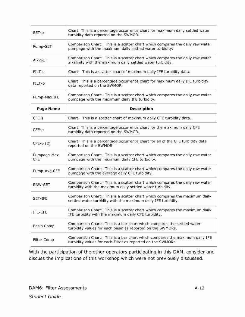
DAM6: Filter Assessments A-12
Student Guide
SET-p Chart: This is a percentage occurrence chart for maximum daily settled water turbidity data reported on the SWMOR.
Pump-SET Comparison Chart: This is a scatter chart which compares the daily raw water pumpage with the maximum daily settled water turbidity.
Alk-SET Comparison Chart: This is a scatter chart which compares the daily raw water alkalinity with the maximum daily settled water turbidity.
FILT-s Chart: This is a scatter-chart of maximum daily IFE turbidity data.
FILT-p Chart: This is a percentage occurrence chart for maximum daily IFE turbidity data reported on the SWMOR.
Pump-Max IFE Comparison Chart: This is a scatter chart which compares the daily raw water pumpage with the maximum daily IFE turbidity.
Page Name Description
CFE-s Chart: This is a scatter-chart of maximum daily CFE turbidity data.
CFE-p Chart: This is a percentage occurrence chart for the maximum daily CFE turbidity data reported on the SWMOR.
CFE-p (2) Chart: This is a percentage occurrence chart for all of the CFE turbidity data reported on the SWMOR.
Pumpage-Max CFE
Comparison Chart: This is a scatter chart which compares the daily raw water pumpage with the maximum daily CFE turbidity.
Pump-Avg CFE Comparison Chart: This is a scatter chart which compares the daily raw water pumpage with the average daily CFE turbidity.
RAW-SET Comparison Chart: This is a scatter chart which compares the daily raw water turbidity with the maximum daily settled water turbidity.
SET-IFE Comparison Chart: This is a scatter chart which compares the maximum daily settled water turbidity with the maximum daily IFE turbidity.
IFE-CFE Comparison Chart: This is a scatter chart which compares the maximum daily IFE turbidity with the maximum daily CFE turbidity.
Basin Comp Comparison Chart: This is a bar chart which compares the settled water turbidity values for each basin as reported on the SWMORs.
Filter Comp Comparison Chart: This is a bar chart which compares the maximum daily IFE turbidity values for each Filter as reported on the SWMORs.
With the participation of the other operators participating in this DAM, consider and discuss the implications of this workshop which were not previously discussed.
DAM6: Filter Assessments A-13
Student Guide
Workshop 4: Conducting a Filter Inspection Format: Practical Exercise
Time: Approximately 4 hours
Trainer: DAM6 trained instructor
Tools/equipment: See the Equipment List, below.
IMPORTANT:
• Extreme caution must be exercised to ensure operator safety, especially in the case of the large filters, where confined spaces and high backwash water flow rates exist.
• Extreme caution is also required to prevent damage to the backwash troughs, filter underdrain and support gravel, and filter media.
• Filter evaluations require a team of at least two licensed water works operators.
Notes: If a system has triggered a filter assessment and is using this training to facilitate compliance with assembling and submitting the filter assessment report, participation in this module will not accomplish this objective unless the following steps are taken prior to participating in the module:
(1) The system must assemble all the equipment needed to conduct this workshop and ensure it is in good working order.
(2) The system must be prepared to perform all of the exercises outlined in this Steps 1 through 9 of this workshop. This includes ensuring that the function of all valves, pumps, water transfer lines, and other filter controls allow completion of the exercises.
(3) If the schedule does not allow completion of all the exercises, some may have to be completed without instructor support.
(4) If special safety equipment is required to ensure operator safety, the system is responsible for providing the equipment and the Class C certified operators trained to use it to conduct these exercises. (The instructor will only provide guidance to the certified operators actually conducting the exercises.)
(5) The operators performing these exercises should read Chapters 4 and 5 of Regulatory Guide 211 (RG211) prior to participating in this DAM.

DAM6: Filter Assessments A-14
Student Guide
(6) The operators participating in this DAM will be responsible for making all notes, recording all pertinent data, and completing the Filter Profile Report and/or Filter Assessment Report.
Equipment Needed:
Equipment required for this workshop must be secured prior to conducting this DAM. Some of the equipment may be locally fabricated (for example the filter probe, the Secchi disk, the hook gauge, etc.). Additionally, the operators may utilize any preferred functional substitute equipment.
Equipment List
No. Item Check
1 One clipboard with preferred paper, writing, and drawing tools
2 One ladder of sufficient reach to allow the operator to safely enter and exit the filter
3 One rope to secure the ladder
4 Safety gear required by local policy and based on operator preference
5 One filter probe with Secchi disk attachment
6 One hook gauge with non-flexible line
7 One 1-inch wide tape measure or a 1-inch wide yardstick
8 Four 2 ft X 2 ft pieces of ¼-inch plywood (Each piece of plywood should be equipped with a rope which can be used as a handle.)
9 One 2 ft X 3 ft piece of ⅜-inch plywood (This should also be equipped with a rope handle.)
10 One stopwatch accurate to 1/10 seconds
11 One 8-foot to 10-foot length of 2x2 or 2x4
12 One 1 ft X 1 ft X 2.5 ft (H) plexiglass excavation box (optional)
13 One calculator
14 Plastic sandwich bags (for media samples)

DAM6: Filter Assessments A-15
Student Guide
15 Camera (optional)

DAM6: Filter Assessments A-16
Student Guide
Workshop 4 Step 1: Prepare a Filter Diagram
Prepare a diagram of the filter showing the location of the filter inlets, outlets, and backwash trough. Although the diagram does not have to be exactly to scale, it is helpful if the diagram is drawn as large as possible and looks like the filter. If necessary to make an accurate diagram, the length and width of the filter bed and the locations of the troughs should be measured for inclusion in the drawing. Examples are shown in the following figures.
Example of a Rectangular Filter Probe Diagram

DAM6: Filter Assessments A-17
Student Guide
Example of a Circular Filter Diagram

DAM6: Filter Assessments A-18
Student Guide
Notes: The diagram will have many details enumerated.
• The outer dimensions of the media surface are recorded. • The filter troughs are drawn in and, where appropriate, the trough spacing is
indicated. • Numbered locations drawn at regular intervals over the filter surface.
o These are locations where the operators intend to probe. o The numbered locations can also be used to identify the places where
the operators decide to perform excavations and special studies. o When practical, the numbering system should be consistent with:
The order in which the filter probes will be performed, or The most logical order for meaningful presentation of the data.
o The operators do not need to perform the probes “in order” but the data collected must be recorded and preserved in a manner consistent with the numbering scheme in the diagram.
• An accurately oriented “north” arrow is drawn, where appropriate, to help the operators identify the numbered locations when doing subsequent analyses.
• The drawing should be large enough to allow the recording of at least two probe measurements (the depth of the media and the reference depth to the gravel or other media support structure). If not large enough a table for recording these data must be assembled to take required notes.
• Notes written on the diagram should be written in a consistent order to facilitate later review and interpretation.
• Photographs taken during the filter evaluation should be logged with information identifying the reason for the photograph, the location on the filter diagram recorded by the photo, etc. Photographs are particularly good for recording some filter anomalies, such as:
o The degree of levelness of the troughs or degradation of the troughs. o The condition of the filter walls and gullet. o The presence of jetting during backwash. o The seepage of filtered water into the drained gullet, if there is a
cross-connection. o Filter cracks or media separation from the filter wall. o Peaks and valleys over the surface of the media.
Workshop 4 - Step 2
Draining the Filter and Measuring Filtration Rate
1. Close the filter influent valve completely. 2. Leave the filter effluent valve open. 3. Record the filtered water flow rate from the filter’s flow meter.

DAM6: Filter Assessments A-19
Student Guide
4. Using the hook gauge, measure and record the amount of time that it takes for the water level to fall six inches. If possible, make this measurement while the water level is at least six inches above the top of the backwash trough. If the water level is not at least six inches above the top of the backwash trough, wait until the water level is below the top of the trough to begin the measurement.
5. Determine and record the wetted surface area of the filter. a. If the drawdown was measured above the wash water trough,
calculate the surface area of the filter. b. If the drawdown was measured below the top but above the bottom of
the trough, determine the total area between the troughs. 6. Calculate (and record) the filtration rate using Equation 1.
Equation 1: Calculating filtration rate:
7. Compare the calculated filtration rate with the filtration rate shown on the filtered water flow meter.
The following procedures are used to prepare for following steps in Workshop 4.
8. Leave the filter effluent valve open until the water reaches the surface of the filter media.
9. While the water in the filter is still falling, use the filtration rate calculated above, to determine how long it will take for the water to descend for the design depth of the filter bed.
10.When the water reaches the surface of the filter media, take one of the two following actions:
a. If there are no filter-to-waste facilities: i. Leave the filter effluent valve open long enough to allow the
water level to descend to the media support structure (if gravel-less) or to the top of the gravel layer (if applicable).
ii. Then, completely close the filter effluent valve. b. If there are filter-to-waste facilities):
iii. Completely close the filter effluent valve.

DAM6: Filter Assessments A-20
Student Guide
iv. Open the filter-to-waste valve. v. Leave the filter-to-waste valve open long enough to allow the
water level to descend to the media support structure (if gravel-less) or to the top of the gravel layer (if applicable).
vi. Completely close the filter-to-waste valve.
Note: The filter-to-waste line typically has less pressure than the filter effluent line. If this is not true, the procedures at Item 10.a. should be used.
Workshop 4 - Step 3
Pre-backwash Filter Bed Examination
IMPORTANT:
This part of the filter evaluation requires an operator to climb down into the filter. Operators must take precautions to avoid injury and filter damage.
• At least two licensed operators should be present any time that an operator enters a filter. One of the operators must carefully enter the filter and make the measurements while the other remains outside the filter to record the data. Class D operators should not enter the filter unless accompanied by a Class C surface water operator.
• Filter surfaces are often wet and slippery . . . any operator who enters the filter must wear slip-resistant footwear.
• If filters are defined as “confined spaces” any operator who enters those filters must follow applicable locally administered confined space entry procedures.
• Operators are encouraged to develop appropriate safety precautions even if the filters are not defined as confined spaces.
• Operators should not stand or walk in the fiberglass backwash troughs because the troughs can be severely damaged.
• The ¼-inch plywood boards should be used to distribute and support the weight of the operator whenever they are walking or standing on the filter media.
1. Lower the ladder into the filter using one of the following procedures:

DAM6: Filter Assessments A-21
Student Guide
a. If the filters are equipped with lightweight fiberglass backwash troughs, the troughs will not support the weight of an individual, and the following procedure is recommended:
i. Lower the ¼-inch plywood into the filter and place it directly on the filter media near the wall where the operator will enter. This board will then be used as the support footing for the ladder.
ii. Lower the ladder into the filter and center its feet on the piece of plywood.
b. If the filters are equipped with concrete or securely mounted steel backwash troughs, the troughs will support the weight of an individual. Consequently, the operators can either use the procedure described in item "a" above, or they can lower the ladder so that its feet are securely positioned directly in or on the backwash trough.
2. Secure the top of the ladder to the top of the filter or the filter railing using a strong rope or chain.
3. If a safety harness is being used, secure the end of the lanyard to the filter railing at a location where the operator standing outside the filter can reach it.
4. The operator who will be making the measurements must carefully enter the filter. The operator who will be recording the data should remain outside the filter as a safety precaution.
5. Lower the tape measure, the ¼-inch plywood pieces, the straight 2x2 or 2X4, and other equipment into the filter.
6. Observe the surface of the filter media for the following media conditions. a. Thickness of the floc mat: Measure the thickness of the floc mat at
several locations throughout the filter. b. Distribution of floc mat: Specifically, look for areas where the floc
has accumulated to an unusual depth or has not accumulated to the same degree as in the rest of the filter.
c. Mudballs: Specifically, look for areas where mudballs appear to be accumulating on the surface of the media.
d. Significant media mounds or depressions: Specifically, look for areas where the depressions or mounds exceed 1½-inches in depth or height.
e. Filter cracks: Specifically, look for cracks that are more than 6-8 inches long, more than ¼-inch wide, or more than ½-inch or so deep. Some small cracks may form as the filter dewaters, but larger cracks suggest that the filter media has been coated with an excessive coagulant layer.
f. Separation from filter wall: Specifically, look for areas where the media has separated from the wall more than ¼ inches, the length of the separation exceeds 6-8 inches, or the separation is more than 1-

DAM6: Filter Assessments A-22
Student Guide
inch deep. Some separation from the filter wall may occur as the filter dewaters, but separations that exist before the filters dewater suggest that the filter media has been coated with an excessive coagulant layer.
7. On the filter diagram, record the location of any unusual conditions seen on the media surface and describe the condition in detail on a separate sheet of paper.
Workshop 4 Step 4: Filter Bed Measurements
Notes:
• Lay the straight 2x2 or 2x4 across the tops of adjacent troughs so that it spans the space between the troughs and provides a level reference point for the measurements between the filter troughs.
• If practical, operators should not stand or walk directly on the surface of the filter media. In any case, they should avoid making footprints at locations where the filter will be probed or excavated.
• Probe measurements of media depth and reference depth are related but the operator has the choice of how to conduct the measurement. The reference measurement may be to the top of the media or the top of the gravel layer. It is just very important that everyone participating know what the measurements mean and how they are recorded for later use.
1. Lower the filter probe into the filter. 2. Keeping the probe perpendicular, probe the filter at two-foot intervals (or as
indicated on the filter diagram). a. Determine the levelness of the media surface by measuring the
distance from the top of the filter trough to the surface of the media. i. Lower the probe until it just touches the top of the filter media. ii. Record the distance (to the nearest inch or less) directly on the
filter diagram. b. Measure the depth of the media bed to the top of the gravel support
layer or, if the filter uses a gravel-less underdrain, to the top of the underdrain.
i. Press the probe down into the media until a change in resistance is felt or until the sound of the probe passing through the media changes.
IMPORTANT:
• Do not push the probe into the gravel layer. Be extremely careful not to press the probe so far down that it damages the filter underdrain.

DAM6: Filter Assessments A-23
Student Guide
• Pressing the probe into the gravel will not damage the filter, but it will make the measurements unreliable.
c. Record the depth (to the nearest inch or less) directly on the filter diagram.
3. Determine levelness of the support gravel/underdrain. a. Either:
i. measure the distance from the top of the backwash trough to the surface of the support gravel or gravel-less underdrain; or
ii. measure the depth of the media layer and the distance from the media surface to the top of the backwash trough and add the two readings.
b. Record the result directly on the filter diagram. 4. Reduce the interval spacing if significant differences are detected between
adjacent measurements for either: 1) the distance to the media surface, or 2) the media depth.
a. If the distance or depth between adjacent measurements varies by more than three inches, make an additional set of measurements at the midpoint between the points.
b. If the distance or depth continues to vary by more than three inches, continue to measure at midpoints until the distance between the measurements is only two inches or less.
5. Probe the filter at each site that an undesirable filter backwash or media surface condition was identified.
Workshop 4 - Step 5
Excavating the Filter
IMPORTANT:
Operators must take some extremely important precautions to avoid injury and filter damage.
• Operators must comply with all prescribed safety requirements.
• Do not disturb the gravel support bed when excavating the media at each site.
Excavation at each site must be stopped as soon as the samples contain more than about 10% gravel (DO NOT excavate the gravel layer).

DAM6: Filter Assessments A-24
Student Guide
The upper 75% of the filter bed can be excavated by hand or with a small shovel.
The lower 25% of the filter bed must be excavated by hand.
• When practical, avoid standing directly on the filter media.
• If the filter design does not allow the filter to be completely drained, excavation below the remaining water level should not be attempted without an excavation box.
Notes: • During the filter excavation, note and record the following information:
o If mudballs are present, note their size and shape and how far they have penetrated into the media bed.
o If the filter contains more than one type of media, note how distinct the interface is between the different media layers, that is, the degree of stratification.
o If the filter contains more than one type of media, note how much intermixing of the media layers is present.
• If the excavation cannot be completed because of the presence of subsurface standing water or other conditions that cause the walls of the excavation hole to collapse, it may be useful, or even necessary, to use the excavation box. Do not force the excavation box so deep that it penetrates into the gravel layer.
• If the operators observe media conditions which would provoke further analyses, media samples should be collected and preserved for subsequent use. The sample should be labeled and the following items should be logged:
o The reason the sample is being collected.
o The location of the sample.
o The depth(s) of the sample.
o The type of sample (composite, sand only, anthracite only, etc.).
Make sure that all of the activities required in Step 4 - Filter Bed Measurements have been completed.
Place the ¼-inch plywood pieces on the filter media about a foot from the area to be excavated.
Clean a three square foot area on the opposite side of the excavation site by scraping off the top ¼-inch of filter media and placing it in a pile on one end of the scraped area.
Excavate a 6-inch to 8-inch diameter hole in the filter bed. Excavate the top three to six inches of the media bed.

a. If mudballs are present, note their size and shape and the depth of penetration.
b. Place the excavated media in a pile at one end of the scraped area. Excavate the remainder of the upper media layer. If mudballs are present, note their size and shape and the depth of
penetration. For example, “pancake-shaped mudballs with a diameter of ½ to ¾ inches have penetrated three inches into the anthracite layer.”
Place this layer of excavated media in a pile adjacent to the previous pile. If the filter contains multiple media materials, describe the interface
between the layers. For example, “14 inches of clean anthracite is located above a two-inch layer of intermixed sand and anthracite that contains about 40% sand and 60% anthracite.”
If the filter bed contains more than one media layer, continue the excavation, that is, repeat steps 5 to 9 until all the layers between the surface of the media and the upper gravel layer have been excavated and described.
Replace the media after completing the excavation. a. Return the media to the hole in the opposite order that it was
removed. That means last out = first in. b. Pack each layer slightly by hand as it is replaced. c. If there is media left over after filling the excavation hole, spread it
around in the general area of the excavation site and the cleared area. Repeat steps 1–11 in each area where unusual backwash or media
conditions were observed or noted during the media probing. Collect “Core Samples,” as described in the Student Text, if any special
studies are to be conducted on the filter media. Remove the filter probe, tape measure, plywood squares, and any other
equipment from the filter. Exit the filter and remove the ladder and the ¼-inch plywood piece if it was used.
Workshop 4 Step 6: Observing the Filter Backwash
IMPORTANT:
During the backwash process, large volumes of water are used and high water velocities exist in the backwash troughs and spent backwash water channel. Consequently, whenever possible, the evaluation team should collect the data required in this step without being in the filter during the backwash cycle. However, if an operator needs to be in the filter during a backwash cycle, the following precautions must be taken to avoid injury.
DAM6: Filter Assessments A-25
Student Guide

DAM6: Filter Assessments A-26
Student Guide
• At least two licensed operators should be present any time that an operator enters a filter. One of the operators must carefully enter the filter and make the measurements while the other remains outside the filter to record the data.
• Filter surfaces are often wet and slippery . . . any operator who enters the filter must wear slip-resistant shoes.
• Any operator who is inside the filter box during a backwash procedure must wear a safety harness that is securely anchored to the filter wall or some other similarly immovable object. The lanyard, or safety rope, must be short enough to prevent the operator from becoming submerged in the filter bed, backwash trough, or spent backwash water channel.
• Operators must stand at a location that will prevent injury or filter damage. Examples MAY include:
The top of the spent backwash water channel wall.
The top of a steel backwash trough where it connects to the wall of the filter box.
• Operators should not stand on the top of fiberglass backwash troughs because they can be severely damaged.
Make sure that all of the activities required in Step 5 have been completed. Open the filter backwash valve slightly and allow that water to rise to a
level that is 6–8 inches below the bottom of the backwash water trough. The rise rate of the water should be only a fraction of the lower backwash rate. This will aid in filling any air-filled voids in the underdrain and media bed with water.
Allow the filter to sit for a short time to allow remaining air to escape. Hand the Secchi disk to the operator who will be making the
measurements. The operator who will be recording the data must remain outside the filter as a safety precaution.
If applicable, find a place to stand that has good footing, and use the lanyard to secure the safety harness to the filter wall or other similarly immovable object.
Complete a routine backwash of the filter following the backwash procedure in the plant’s routine filter backwash procedure.
Determine if there are any unusual backwash conditions, such as described in Subsection 3.1.4 of the Student Text. These conditions might include:

a. Levelness of the backwash trough: Specifically, look at the top of the backwash water troughs to determine if water flows over some sections of the trough sooner than others.
b. Trough flooding: Specifically, look for areas where flooding is occurring in one or more of the troughs.
c. Media boils and jets: Specifically, look for areas where the backwash process is producing a significantly more vigorous rolling action in the media. Pay particular attention to areas along the filter wall.
d. Media loss: Specifically, look for media carryover into the backwash water troughs. Pay particular attention to areas where the carryover appears to be localized.
e. Lack of media agitation: Specifically, look for areas where the media is moving very little. Again, pay particular attention to the areas along the filter wall and in the corners of the filter.
Record the location of any undesirable backwash conditions on the filter diagram, and describe the condition in detail on a separate sheet of paper.
Note: The measurement of the bed expansion and the measurement of the backwash rise rate must be done when the highest backwash rate is being used. It is also essential that the backwash rise rate measurement be performed when the surface of the rising backwash water is below the troughs or when the backwash to waste valve is closed and the entire gullet is full to the level of the water above the troughs. These requirements almost certainly will require the operators to deviate from their normal backwash protocol. However, the bed expansion and backwash rise rate measurements do not have to be performed in the order presented here.
Measure the height of the expanded media bed at the maximum backwash flow rate routinely used during the backwash cycle.
a. Lower a Secchi disk into the filter media until a small amount of filter media from the expanded bed begins collecting on the top of the disk.
b. Measure the distance from the top of the filter wall to the surface of the fluidized (that is, expanded) media bed.
c. Record the result on the filter diagram. d. After the backwash is complete, perform the unexpanded bed
measurement as described in item 14, below. Measure the maximum backwash water flow rate routinely used to
backwash the filters. a. At the maximum backwash water flow rate, record the flow rate that is
being shown on the backwash water flow meter. b. At the maximum backwash water flow rate, close the backwash waste
drain valve.
DAM6: Filter Assessments A-27
Student Guide

c. Using the hook gauge, measure and record the amount of time that it takes for the water level in to rise six inches. (If there is a filter gullet, the filter gullet must be full to get this measurement.)
Open the backwash waste valve. Complete the backwash cycle as described in the backwash procedure. Return the filter to service using the procedure described in the backwash
procedure. Measure the height of the unexpanded filter bed using the same process as
described in Item 9, above.
Note: The height as read on the probe with the Secchi disk will be larger in magnitude as measured from the top of the filter wall to which the operator is comparing the two measurements.
Calculate backwash water flow rate using Equation 2.
Note: The surface area used in Equation 2 may be the surface area of the media or the surface are of the media plus the surface area of the filter gullet.
DAM6: Filter Assessments A-28
Student Guide
Equation 2: Calculating the backwash water flow rate
Calculate the percent bed expansion using equation 3.
Equation 3: Calculating the Percent bed expansion

DAM6: Filter Assessments A-29
Student Guide
Workshop 4 - Step 7
Observing the Post-backwash Surface of the Filter Media
After a complete backwash, the filter is in a “clean” condition. The water above the filter media should be at the level of the backwash troughs and should be relatively clear. The operators should be able to perform a fairly complete examination of the post-backwash condition of the filter surface prior to opening the settled water influent valve.
1. Repeat the inspection process described in Workshop 4 - Step 3. 2. Using the filter diagram, record the location of any unusual conditions seen
on the media surface, and describe the condition in detail on a separate sheet of paper.
Workshop 4 - Step 8
Data Interpretation
Note: If the system has triggered a filter profile or filter assessment, the information gathered during the filter evaluation may have to be assembled in a prescribed way and must be reported to the TCEQ with the monthly SWMOR. Full details are provided in Chapters 4 and 5 of RG211.
The data, drawings, photographs, and other notes collected during the preceding exercise represent a large quantity of information about the filter that cannot be assembled in a systematic way without doing a filter evaluation. Some interpretation of these data can be accomplished by an experienced operator. For example:
• If backwash water is observed to flow into one backwash trough before another trough, the troughs are not level and do not meet TCEQ design standards.
• If the depth of the media is significantly less than indicated in the TCEQ approved design, the filter may not be removing turbidity as well as it should or may have shorter filter runs than it would if the filter were maintained as it should be.
• The presence of mudballs in the filter media indicate that the filter backwash is not as effective as desired. (The presence of mudballs, alone, does not indicate why the filter backwash is not effective.)
However, a full interpretation of the information requires study, thought, and some experience. The operators completing this DAM are referred to Sections 3 and 4 of the Student Text to more fully interpret the information they have collected. The

DAM6: Filter Assessments A-30
Student Guide
Student Text was assembled based on the combined experience of TCEQ staff and the many of the operators with whom it has been our privilege to learn from and to work with for many years.
Workshop 4 - Step 9
Observing the Post-Backwash Filter Performance
Note: If the system has triggered a filter profile, the post-backwash filter performance may have to be reported to the TCEQ with the monthly SWMOR in accordance with RG211. Further details are provided in Chapter 4 of RG211.
The filter should be returned to service following the backwash in accordance with the plants routine filter backwash procedure. Because some plants provide a period of idle time before returning the filter to service, this step is not included as a normal step in this workshop. However, the operators are encouraged to review:
• Subsection 2.3.1.4 (entitled “Idealized Turbidity Profile for a Filter Run”); • Subsection 2.3.1.5 (entitled “Analyzing Filter Run Data”); and • Subsection 2.3.1.6 (entitled “Post-Backwash Turbidity Spikes”)
of the Student Text and apply those principles to a post-backwash evaluation for one or more of their filters. These analyses may be used to provide more definition to your filter evaluation.

DAM6: Filter Assessments A-31
Student Guide

DAM6: Filter Assessments B-1
Student Guide
Appendix B: Filter Maintenance Guidelines This appendix contains a generic filter maintenance standard operating procedure, adapted from a document provided by Leopold, Inc.11 Please note that the organization of the text has not changed other than to reformat the original to fit in this appendix. Some of the subtopics referred to herein are not included in this document, as they are contained in other Leopold documents. Further, the TCEQ offers no warrantee as to the effectiveness of any protocol described in this appendix.
Filter Bed Inspection The purpose of performing general operational inspections is to maintain an ongoing visual process of evaluating filter performance and bed conditions. A program should be in place to observe every filter during the operation/backwash cycle. This should be done by maintaining a list of all filters in the control room with the following data to be recorded:
• Inspector
• Date
• Comments
A visual inspection allows the operator to determine if the backwash sequence needs to be modified or if problems may exist in the filtration cycle. A recommended inspection schedule is included in the appendix. Key aspects of this inspection process are as follows:
1. Review Foam Abatement Operation (if used)
• Evaluate foam abatement effectiveness and filter wall cleanliness
• Evaluate over spray problems that may create corrosion problems
• Evaluate general operational failures (if any)
2. General Observation of Filter Operations
• Proper inflow/outflow conditions .
11 This draft SOP is used with permission.

DAM6: Filter Assessments B-2
Student Guide
• Evaluate valve operation for leaks and cycle times
• The valves should operate slowly and smoothly
3. Drain the Filter and Evaluate the Surface Wash System (if used)
• Check for blown nozzles
• Check for nozzle erosion
• Check for plugging of nozzles
• Check for cracked or broken nozzles or structural supports
• Evaluate rotary system operations (if used) – bearing wear and speed
• Proper pressure and flow rate during normal operation
4. Evaluate Other Structural Components
• Wash troughs-leaks, cracks, and levelness of weirs
• Valving-leaks, speed and smoothness of operation
• Baffling-structural integrity, effectiveness
• Sampling system-location and proper operation
• Piping Systems (mechanical and electrical)
5. Media Inspection (refer also to the section on “Media Condition” in the Filtration Design Manual.
• Unevenness
• Mudballs or side wall cracking
• Improper debris in filter
• Unacceptable amount of silt algae, etc. on surface
6. Fines
Fines will accumulate on the surface of the media over time, as discussed previously. Therefore, an inspection for fines should be made at least every three months or until a confidence level is reached.
• Drain the filter down below the media surface. Using a square edged shovel, make a cut straight down into the media. Then, make another cut at an angle to that and lift out a section of the media as shown in Figure 1.
• If fines are present, it’ will be easy to see them on the surface. They will be in a thin layer, usually 1/8” or 1/16” or less. Below that it will be very evident
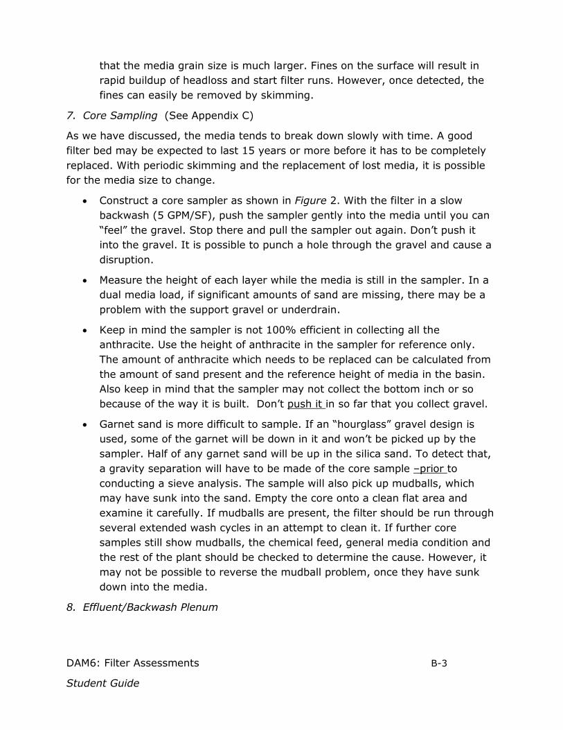
DAM6: Filter Assessments B-3
Student Guide
that the media grain size is much larger. Fines on the surface will result in rapid buildup of headloss and start filter runs. However, once detected, the fines can easily be removed by skimming.
7. Core Sampling (See Appendix C)
As we have discussed, the media tends to break down slowly with time. A good filter bed may be expected to last 15 years or more before it has to be completely replaced. With periodic skimming and the replacement of lost media, it is possible for the media size to change.
• Construct a core sampler as shown in Figure 2. With the filter in a slow backwash (5 GPM/SF), push the sampler gently into the media until you can “feel” the gravel. Stop there and pull the sampler out again. Don’t push it into the gravel. It is possible to punch a hole through the gravel and cause a disruption.
• Measure the height of each layer while the media is still in the sampler. In a dual media load, if significant amounts of sand are missing, there may be a problem with the support gravel or underdrain.
• Keep in mind the sampler is not 100% efficient in collecting all the anthracite. Use the height of anthracite in the sampler for reference only. The amount of anthracite which needs to be replaced can be calculated from the amount of sand present and the reference height of media in the basin. Also keep in mind that the sampler may not collect the bottom inch or so because of the way it is built. Don’t push it in so far that you collect gravel.
• Garnet sand is more difficult to sample. If an “hourglass” gravel design is used, some of the garnet will be down in it and won’t be picked up by the sampler. Half of any garnet sand will be up in the silica sand. To detect that, a gravity separation will have to be made of the core sample –prior to conducting a sieve analysis. The sample will also pick up mudballs, which may have sunk into the sand. Empty the core onto a clean flat area and examine it carefully. If mudballs are present, the filter should be run through several extended wash cycles in an attempt to clean it. If further core samples still show mudballs, the chemical feed, general media condition and the rest of the plant should be checked to determine the cause. However, it may not be possible to reverse the mudball problem, once they have sunk down into the media.
8. Effluent/Backwash Plenum

DAM6: Filter Assessments B-4
Student Guide
If possible, it is recommended that the eft1uent/backwash plenum be periodically inspected. At the same time, the exposed underdrain in that area could also be inspected. Deposits of mud, gravel or media in this area would be of major concern. The erosion of grout and/or concrete would also be of concern
The clearwell (treated water storage tank) should be inspected in a similar manner. The presence of media or gravel is an indication of an upset filter. Mud could also mean an upset filter. However, it could also be caused by improper chemical feed, or turbulence causing floc to be broken up and pass through the filter.
Filter Media Cleanliness The purpose of the filter media cleanliness test “is to provide a quantitative evaluation of filter media backwash effectiveness and overall system performance”. Maintaining filter cleanliness, with the established parameters, helps to optimize the backwash/filtration process.
1. Evaluation Process
Core samples of the filter media are taken for determination of accumulated solids per volume of filter media. The condition of the filter media is rated based on the percent of accumulated solids in the media. The amount of solids remaining in the media, after backwash, is indicative of the efficiency of the backwash cycle and of the overall system performance. Filter media cleanliness testing results can be used as a method for evaluating plant and filter operational effectiveness and as a tool to improve filter performance. Key factors to be evaluated include the following:
• Optimizing parameters such as frequency and length of the backwash and surface wash process
• Efficient use of rise-rates (backwash rate)
• Primary, filter and/or backwash chemical coagulation dosages
• Efficient use of surface foam abatement sprinklers (if used)
• Optimizing the efficiency of the pre-filter sedimentation process
• Addressing all of the filter bed conditions noted in this program
2. Core Sampling Procedure (Also see the references to Core Sampling above and in Appendix C)
During the last minute of backwash, take an in-depth core sample of the filter media. A sample of all filter media material is required (coal, sand, garnet, etc.)

DAM6: Filter Assessments B-5
Student Guide
• Take a representative portion of the core sample for analysis of accumulated solids
• Wash media, filter and weigh solids
• Record sample area locations filter
3. Filter Media Condition
Percent Weight of Accumulated Solids
Condition of
Filter Media
Recommended Media
Sampling Frequency
0.00 - 0.005 excellent yearly
0.006 - .010 very good yearly
0.011 - .025 good yearly
0.026 - .050 fair twice yearly
0.051 - 0.10 poor quarterly
0.10 - 0.20 Bad monthly
over 0.20 Very bad twice monthly
It should be remembered that the condition of filter media, determined by this method, represents a very small portion of the total filter media. The test results can be much more representative of the overall filter media condition if more than one filter is sampled. Moreover, this test should be performed in conjunction with visual observation during the backwash operations to determine the clarity and analyses of the filter backwash water (turbidity and/or suspended solids). Additional filter performance testing such as media expansion, rise rate, backwash sequence timing should be adjusted to improve backwash efficiency
Skimming The purpose for scraping the surface of the filter media is to remove accumulated fines that are below the specified standards.
Fines are generated by the inherent backwashing process, water energy and physical media abrasive impacts. The agitation process naturally breaks up media

DAM6: Filter Assessments B-6
Student Guide
slowly over time. The broken media, which is smaller and lighter, will rise to the surface.
If these fines are not removed by the backwash operation and are allowed to accumulate on the bed surface, a greater proportion of the incoming turbidity loading will be filtered or strained on the surface. Shortened filter runs, reduced filtration effectiveness and solids storage capacity will result. Also, there is greater change for break-through to occur, once the hydraulic loading force exceeds the straining resistance.
In order to minimize surface filter straining and enhance in-depth filtration and optimize filter performance, it is important to remove these fines by scraping or skimming. The media surface should be inspected for fines every 3 months or as experience dictates. For 1 mm anthracite, the screens normally used to evaluate samples are as follows:
Sieve Designation
(US Series)
No 10 .
Sieve Opening (mm)
2.00
12 1.68
14 1.41
18 1.00
20 0.841
25 0.707
Referring to the sieve analysis in Figure 3, the effective size is 1.01 mm. Approximately 5% of new material is skimmed off. That point would fall in between the No. 18 and No. 20 screens.
For skimming during normal maintenance, a visual inspection should be done as well as a sieve analysis. In this case, all material finer than a No. 20 screen should be skimmed off.
In order to skim the filter, drain the water level down well below the media. Place boards on the media to walk on. Otherwise the fines will be pushed down into the bed, as the workers walk on it.
DAM6: Filter Assessments B-7
Student Guide
Equipment required (per worker)
• 1-2 walking boards (12 x 24 x 3/4 inch min.)
• Square edged shovel or skimming pan
Using the shovel or pan, skim the specified thickness off the top. Discard the material into the waste trough or into buckets for removal as site conditions dictate.
It is important that the skimming procedure be done by collecting the material in the shovel or pan with a scooping type motion. Do not push, scrape or roll the fines. That is not as efficient and will only serve to punch some of the fines down into the bed.
Once the skimming operation is completed, backwash the filter and check for fines again per paragraph A6. It may be necessary to skim more than once to remove all the fines.
Whenever working in a filter, be sure to count all the tools, walking boards and other implements. Then, when the work is done, make sure that everything is accounted for. It is not uncommon for shovels and other tools to be lost in filters.
Filter Bed Expansion Insufficient filter media expansion can result in accumulated materials, beyond a desired loading amount. The filter will lose operational efficiency due to reduced bed storage capacity, which will cause shorter run times; a greater volume of backwash water required and will increase plant effluent turbidity. Metropolitan has established 20-30% expansion range for the filtering media (coal, sand, and garnet) as the optimal expansion range for the backwash process. Poor bed conditions such as significant anthracite loss will significantly impact bed expansion capabilities and filter performance.
The proper rise rate or backwash flow is essential in cleaning the media. However, it does not follow that the higher the rate the better the scouring action. The proper rates are determined by experimentation and are usually somewhat less than complete fluidization. Rise rates in the range of 15-20 GPM/SF (24-32 inches per minute) are normal for 1 mm anthracite.
1. Measurement
Media expansion, during backwash is usually expressed as a percentage of the overall bed depth, excluding gravel.

DAM6: Filter Assessments B-8
Student Guide
There are two basic methods of determining the amount of media expansion in backwash; direct measurement and by pilot columns.
a. Direct Measurement
For direct measurement, make a brightly colored "target" out of thin metal or wood and affix it to the end of a measuring rod per Figure 4. Place the filter into backwash. Toward the end of the cycle, when the water is clean, push the rod down into the filter. Stop when the "target" can be seen to reach the top of expanded media. Then, measure the depth of the rod to the walkway or some other reference point. Record that measurement and place the filter back into service. Once the backwash cycle is over, the media will settle back into place. However, it will still be in a slightly "fluffed up" condition. The filter needs to run for at least an hour to compact the media down to its normal operational level. At that point, another measurement should be taken by setting the rod and target down on the media. The expansion is than calculated as follows:
Measurement Procedure - This process should be performed weekly to maintain optimum backwash efficiency.
• Place filter bed in backwash, record water temperature and sample dissolved oxygen. If the dissolved oxygen is high, it may be necessary to backwash frequently to prevent the oxygen from coming out of solution. If it comes out of solution, it will create an artificially high headloss and carry out media during backwash.
• Measure the height of the filter media using the measuring rod, photocell or other approved measuring device during the last minute of backwash. Record this measurement "A".
• Before the backwash or 1 hour after returning to service, measure the media elevation and record that as measurement "B".
• Calculate expansion by subtracting "B" from "A" as noted:
Bed Expansion % = A – B X 100
Media depth
Example: Bed Expansion % = 4” – 2” X 100 = 7.1%
28”
Corrective Procedure - If the bed expansion is low, as noted in the previous example (7.1 %), the backwash rate should be increased and the unit may need to be cleaned. If the unit does not have a mudball, or side wall mounding problem and

DAM6: Filter Assessments B-9
Student Guide
the surface wash system is working properly, increasing the backwash rate to deliver the proper expansion should be sufficient to clean the media.
NOTE: An exception to this procedure would be for coarse monomedia using air scour. In that case, a sub-fluidizing wash rate will be used and a solids analysis would be required to determine media cleanliness.
Each time the rate is increased, make sure no launder flooding or excessive coal loss is occurring. Remeasure the bed as before, to determine if the established expansion range has been achieved. If not, increase the rate again and repeat the procedure. If the maximum available rate does not produce the desired expansion the media should be checked for effective size by core sample and sieve analysis. If enough anthracite has been lost to change the effective size, it may not be possible to expand it properly.
After a series of high rise rate washes, a backwash rise rate and time duration should be established to clean the beds and attain the desirable expansion range.
Discussion/Interpretation - The use of bed expansion as a determining factor for backwash efficiency should be a part of a filter performance program: Variables that do affect media expansion are as follows:
• Media cleanliness
• Media grain size
• Media binding (coagulants, organic matter)
• Water temperature
• Rise rate
• Dissolved oxygen
All of these variables should be recorded during the time of measurement(s) to achieve a reliable, consistent program.
The expansion percentage is normally in the range of 20-30 percent depending on the media type, service, and backwash methods used.
b. Pilot Column Measurement
A permanent pilot column can be used to measure the backwash expansion, as previously discussed. The same media load is used along with the same filtration and backwash flow rates. The expansion can be measured directly using permanent marks on the column for the operational level of the media. Marks can also be placed on the column showing the specified distance normally expected.

DAM6: Filter Assessments B-10
Student Guide
The media expansion is normally determined in the design stage of a project, but can usually be modified by the operational staff. However, it is subject to change depending on the media condition. For example, if there are operational problems such as uncontrolled air, an excessive amount of media can be lost. The media can become coarser if the upper part of the bed is blown out.
If that happens, the media will not expand as much as expected for a given flow rate. Periodic core samples will give an indication of that along with the expansion measurements compared with flow rates.
Pilot columns have the added benefit of allowing the operator to see the entire bed depth.
Measurements can be taken of the expansion of "each separate media types. One factor in the selection of medias to be used together is their compatibility in backwash. If one were too coarse for the other, it would not expand as much as the other. The operator can verify that both are expanded properly at the same time. The direct measurement method is limited to measuring the entire bed expansion.
Backwash Rise Rate Adjustments The rise rate, or backwash flow can be adjusted using several different criteria; temperature, expansion measurement or calculated or measured flow rates.
Temperature
A backwash curve can be developed by adjusting the flow rate to produce the desired expansion at different water temperatures. The results are then plotted in a manner similar to Figure 5. The operator can then set the backwash rate to match the water temperature. Pilot columns are very useful in developing information of this type.
Expansion Measurements
Expansion measurements can be used to verify the proper backwash rate, as discussed previously. However, for this method to be very accurate, the actual media condition must be consistent with the design. Periodic core samples must be taken to verify the media effective size and uniformity coefficient
Calculated Rise Rate
If there is no backwash flow meter, the rate can be calculated by observing the water level rise rate. Use a tape measure and record the distance the water level rises in one minute.

DAM6: Filter Assessments B-11
Student Guide
Water volume = 7.48 gallons
Cubic foot
Backwash flow (GPM/SF) = rise rate (ft/min) X 7.48 gallons (8)
Cubic foot
Total backwash flow (GPM) = GPM/SF x area (SF) (9)
Adjustments should be made to the flow rate to match the required expansion. Here again, periodic core samples should be used to verify the media ES and UC.
The use of this method requires that the water level would be lowered prior to starting the backwash cycle. Adequate height from that level to the bottom of the wash trough must be available after the maximum rate is reached for the measurements to make this method viable. It is also possible to measure the backwash rates by measuring the height of water over the backwash troughs. However, it is not easy to do accurately and is usually not considered.
Placing a Filter ln/Out of Service a. If a filter is to be taken out of service, with the media in place, the basin should be kept full of water. The design of support gravel is based on the fact that wet media "bridges" and will sit on top of much coarser gravel. For example, O.5mm sand will sit on top of 1/8" gravel (3.25mm) if wet. However, if it is allowed to dry out, the sand will leak down through the gravel creating the potential for an upset condition or a plugged underdrain.
Since the filter will be full of water, it should be chlorinated frequently to prevent biological growths which could foul the media.
b. If a filter has been offline for an extended period, it should be backwashed prior to being placed back in, service. Care should be taken to insure that the filter is clean after the backwash and that excess chlorine is washed out. The filter should then be drained and a visual inspection conducted of the surface. All extraneous matter should be removed and the surface should be inspected for dirt or fines. It may be necessary to skim the surface if significant amounts of airborne dirt or bird feathers, etc., have been blown in.
Anytime the filter has been dry during media installation, skimming or other maintenance operations, the basin should be refilled slowly with backwash water. The intent is to slowly drive out the air which has filled the voids between

DAM6: Filter Assessments B-12
Student Guide
the media grains. A rate not to exceed 5 GPM/SF should be used. Otherwise, entrained air can shorten filter runs or blow media out as with uncontrolled air.
Filter Bed Media Stock Measuring The purpose for determining the filter media stock is to insure that sufficient media is in the filter bed to allow proper and efficient in-depth filtration. The proper media depth must be available to provide the desired filtration efficiency and solids storage. The actual media depth is especially critical in filters with shallow media heights and for surface wash applications. The media should be within two inches of the surface washer for maximum efficiency.
1. Establish a Program
A guideline of limiting coal loss to a maximum of two inches should be established prior to the addition of replacement material. It is suggested that coal be added to a filter when the measured coal loss is between 1.5 and 2.0 inches.
Procedure - To insure that filters do not sustain a loss of more than two inches of filter media, a program should be established requiring operators to observe backwash operations and make height measurements. This type of visual inspection program can quickly determine if an excessive amount of coal is being lost and can also be used to check on other factors such as uncontrolled air.
A program for measuring the filter media elevation should be performed at least twice per year on every filter, or more often if the coal loss is higher than desired. If excessive coal loss is occurring, a complete evaluation of the plant should be performed to identify and to eliminate that problem. Coal loss should be kept to a minimum of one inch per year or less, if possible.
A minimum number of measurement points for each filter needs to be established. These points should be specifically documented for historical comparisons. This data should be noted in the filter historical record book.
2. Measuring the Media Depth
The specific measuring process should be as follows:
• The filter being measured should be in service so that the media will be compacted normally.
• All measurements are to be made from specific walkway reference points at each filter (Figure 6). From each reference point, a measurement is taken to the top of the filter media. Four to six measurements should be taken, one at

DAM6: Filter Assessments B-13
Student Guide
each specific reference point per filter. An average media height should then be calculated.
• At each location, the distance to the media should be compared to the average reference walkway elevation to arrive at the elevation of the top of the media.
• The calculated elevation is then subtracted from the specified media or coal surface elevation to determine the loss of media. If a gain is found, this would indicate a build-up of material in the filters, including possible mudballs.
• The equipment used to measure the media height can be either the expansion gauge shown in Figure - or a more permanent device such as a boom with a metal measurement tape and reel attached to the boom. The boom can be attached to the hand railings surrounding the filter, or to some part of the structure which allows access to the filter media.
• Records should be kept on each filter bed coal loss history on standardized forms. If the backwash process is working properly, a consistent loss pattern should be historically established. Any significant deviation is a clue for further investigation and evaluation.
3. Calculations
Sample Records
Reference point = 1442.50
Specification Elevations;
Top of Coal = 1442.40
Media Base = 1420.73
Media Depth = 1.67 ft
= 20 inches
If the actual height is less than desired, the filters will have to be "topped off' by adding new material. The amount of new material to be added is calculated as follows:
Assume a filter 20 feet wide by 20 feet long
Assume a deficit of 2 inches of anthracite
Quantity = 2 inches X 20' X 20' = 66.7 cubic feet

DAM6: Filter Assessments B-14
Student Guide
12 inches/ft
When ordering new material, keep in mind that specific gravity and bulk density vary from supplier to supplier. Typical values are as follows:
Bulk Density Volume
Material lbs./cubic foot CF/Ton v
Sand 100 20
Anthracite (wet) 54-56 35-37
Anthracite (dry) 50 40
Filter sand is usually produced dry and is, therefore, fairly consistent. However, with anthracite, that is not the case. A ton of wet anthracite will have approximately 37 cubic feet per ton whereas the dry material will have 40 cubic feet per ton. Therefore, it is important when ordering media, to specify the volume required and not the weight.
Another factor to keep in mind when ordering anthracite is the "fluff'”. When anthracite is shipped, it contains a variety of particle sizes which are uniformly mixed up in the bag. However, when it is installed and backwashed, the finer material will come to the-top and form its own layer instead of being mixed in with the coarser material. It will then "fluff up" and occupy a volume as much as 10% greater. The "fluff' is a significant factor when replacing the entire bed. When ordering replacement material, specify the exact quantity required. The "fluff' will provide sufficient material for a skimming allowance.
4. Topping Off
When "topping off' add the replacement material first. Then, backwash and skim. That way, the fines from the new material and the old will be removed at the same time.
• When adding replacement materials, it is not necessary to spread it out and level it. Simply dump it in through several feet of water to cushion the fall. If superbags are used, dump in onto a "splash board" and then into the water. A backwash cycle will flatten and level it as well as classifying it.
• Anthracite will absorb 4-5% of its weight in water. If there is little room for media expansion, any new anthracite should soak for 24 hours prior to being backwashed. The lower density of dry anthracite may be such that some of it could wash out.
DAM6: Filter Assessments B-15
Student Guide
Filter Turbidity and Headloss Analyses The purpose of continuous monitoring of filter effluent turbidity and headloss is twofold:
• To ascertain that the water quality and health standards are being met
• To optimize the performance of the filtration process
Backwash turbidity is also monitored to determine the optimum time to terminate the backwash. It is desired to minimize washwater usage and to minimize turbidity spikes when initiating the filtration cycle.
It is also necessary to establish formal calibration guidelines and procedures to ensure the data being recorded or indicated for filtration performance -is reliable and accurate.
1. Monitoring of Turbidity and Headloss
Monitoring of turbidity and headloss is accomplished by means of continuous charge recordings or computerized trending for each filter by turbidity and water quality monitors. Each filter will possess instrumentation (on-line turbidimeter) for measuring continuous filter effluent turbidity and differential pressure equipment for measuring headloss. - Monitoring backwash water turbidity is an optional method for determining when the media is clean.
It is essential that this data be reviewed on a continuous basis, by shift operators and periodically by the laboratory staff and operations supervision. This should be done to insure that maximum filtration effectiveness is being achieved.
2. Calibration
To insure that the data is correct, it is essential that filtration system instrumentation be calibrated weekly by using the manufacturers and recommended calibration procedures.
• First, the plants laboratory turbidimeter must be calibrated using its established calibration procedures. This unit may also be compared with control laboratory units periodically to verify accuracy (if available).
• Second, each filter unit turbidimeter is then calibrated using its procedures against the standard laboratory unit. Additional calibration will be performed until these units are within an established acceptable range. Deviations from acceptable instrumentation guideline standards must be reported to the operators and laboratory personnel. In order to attain the highest level of accuracy and' reliability, instrumentation personnel must make every effort

DAM6: Filter Assessments B-16
Student Guide
to prevent activities not associated with production of water quality information from creating false and negative data. Examples would be spikes caused by flow surges, power failures, etc.
• Weekly calibration tests should be reported to the plant operator for recording in the plant operators log book.
3. Observation/Interpretation
Turbidity and headloss graphs should be available for continuous monitoring, observation and interpretation by plant operators and laboratory personnel. Key filtration parameters that should be monitored and evaluated are as follows:
The filter effluent turbidity trend, during the filtration cycle, can be very helpful for the plant operators, in evaluating filtration performance. Coagulation effectiveness, hydraulic and solids loading, and the media condition will determine the efficiency of filtration and the shape or slope of the turbidity and headloss curves.
For example, a rather lengthy gradual downward turbidity slope following the initial spike in turbidity would be indicative of proper ripening of the" filter and favorable filtration. It could also indicate that operational practices and bed conditions are proper. Whereas, a gradual upward turbidity slope, following the spike could indicate break-through due to poor coagulation, poor ripening and/or possibly poor bed conditions.
The filter headloss trend, during the filtration cycle is also very important in evaluating filter operational effectiveness. A slow gradual rise in the headloss curve, throughout the filtration cycle, indicates proper in-depth filtration, proper coagulation, and good bed conditions, etc.
A more rapid rise in headloss may indicate surface filtration, a rapid increase in hydraulic loading, a poor bed condition prior to initiating the filtration cycle, or poor coagulation.
If an abnormal headloss rise or spike type -rise condition occurs, a potential break-through condition exists. If only one filter is experiencing this problem, the unit should be removed from service, backwashed and a general filter inspection made. If everything seems normal, the unit can be placed back in service, but closely monitored. If the problem recurs, the unit should be removed from service for an in-depth dry bed inspection as well as further chemical feed system evaluations. If all or most filtration 'units are experiencing this problem, this would tend to indicate an unacceptable coagulation condition. This requires an immediate decision to adjust chemical feeds, perform a jar test and reduce flows if necessary.

DAM6: Filter Assessments B-17
Student Guide
Headloss is dependent upon the physical features of the bed, underdrain systems, filter media sizing, filtration rates and the specific character of the applied solids loading. Every operator should be knowledgeable concerning the designed minimum filter headloss and initial operations headloss conditions, in order to effectively evaluate filter operations.
Ideally the headloss should gradually increase. The filtration efficiency should gradually improve and then deteriorate rapidly at the breakthrough point. If this is not occurring, investigations in one or all parameters should be made. Familiarity with the turbidity and headloss curves should serve to alert the shift operators when unusual or poor variations are occurring. They should then consider changes in operational parameters and possibly an investigation into filter bed conditions. In addition, the operator should always evaluate the chemical feed concentrations and effectiveness by jar testing.
Length of filter runs
The length (time) of filter runs is important in determining filter performance. If the run time is shorter than usual, an investigation should be made to determine the cause. Also, it is important to terminate filter run times far ahead of filter break-through conditions. Moreover, keep in mind that water is dynamic and adjustments may be necessary when significant changes in filtration rates, water quality and/or treatment occur. The plant operators should have this data at their disposal for review to assist them in making necessary adjustments.
Filter turbidity breakthrough
Breakthrough may be described as a rapid rise in filter effluent turbidity which exceeds the prescribed limits. Under normal conditions, there is a small turbidity spike when a filter is first placed into service followed by a rapid improvement. Then, if the filter is allowed to run long enough a large spike will occur to which should terminate the run because of the accumulation of an excess amount of solids.
Abnormal breakthrough normally occurs when; I) poor coagulation exists, 2) sudden significant changes in filtration rates occur, 3) excessive headloss is experienced, 4) rapid changes in source water quality, 5) disruption of media is experienced, 6) excessive mudball or clogging is present.
If a breakthrough is causing unacceptable turbidities, the filter bed or beds experiencing this characteristic must be removed from service immediately (unless it was a momentary spike) and the filter(s) backwashed.

DAM6: Filter Assessments B-18
Student Guide
It is essential that a preliminary review of a filter occur before it is placed back into operation. If, upon returning a unit to service, breakthrough continues, a filter should be taken out of service for an in-depth inspection. If there are no apparent physical defects in the filter unit (surface wash problems, media disruption, mudballs, backwash operations deficiencies, etc.), then attention should be given to modifying the chemical dosage being applied.
On occasion, due to rapid increases in filtration rates (accelerated shearing forces) or changes in water quality (material loading), a filter bed may become unstable and a breakthrough condition may be experienced.
Rapid increases in hydraulic loading should be avoided to the extent possible. Secondly, chemical feed changes should be made just before or during the hydraulic changes, not afterward. This will help prevent a poor coagulation condition which is critical to favorable filtration. However, the best method is to have the chemicals flow paced to automatically track any changes.
A unique problem faced by Metropolitan is the possibility of fluidization of all the filter media. During an earthquake, this would cause a temporary spike, unless the gravel becomes disturbed.
Filter effluent turbidity spiking after initiating the filtration cycle
The height and length of turbidity spiking after initiating the filtration cycle will affect water quality and may affect the filter unit’s ability to comply with the effluent requirements. Graphs that show the in-service turbidity spike against time should be available for operator viewing.
A rather short-lived, low level turbidity spike (i.e., less than 0.5 NTU after four hours of operation) is the maximum accepted by some requirements. If a filter effluent turbidity exceeds the recommended guidelines, the operator should immediately remove the filter from service, and begin to review various conditions that may be creating this problem. Activities required are; inspection, corrective actions, and performing operational testing.
Coagulant chemicals applied to the last portion of the backwash cycle could be helpful to diminish the spike (if possible). Applying a coagulant during the final 30~60 seconds of the backwash, to enhance early filtration performance for spike reduction and the attachment process is an effective approach which has been used in some plants.
In-depth filter turbidity and headloss treading, if available

DAM6: Filter Assessments B-19
Student Guide
Trending is useful in determining filter media penetration and optimizing filtration performance. Media zones where maximum turbidity removal and headloss is occurring can be determined. This data could be useful to the plant operator in early prediction of turbidity breakthrough and when to initiate backwash. Also, the type of filtration attachment mechanisms could be reflected in the in-depth turbidity and headloss. Negative head pressure and air binding could also be determined by in-depth filter monitoring.
The data is obtained by installing porous probes at various media depths or by pilot column studies. Turbidimeters and differential pressure instrumentation are connected to the probes and the corresponding signals relayed to the computerized control center for monitoring and making operational adjustments.
A particular depth may reflect high turbidity headloss due to particle sizing and/or floc sizing and penetration. With experience, an operator can use this information to more effectively enhance filtration performance.
Optimization of some or all of the above conditions cannot, to some extent be achieved without considering overall plant operations (i.e., plant flow demands, impacts of one process change on another, filtration rates, turbidity loading, backwash after operations, coagulant dosage and type, air binding, etc.). However, every reasonable effort must be made to optimize filtration performance.
Guidelines for Working in a Filter
The purpose of establishing procedures for working in a filter bed is to prevent the disruption of the support gravel, and in some cases, the filter media.
The recommended procedure is as follows:
• Drain the filter, well below the, media surface. Wet media won't support any weight.
• Lock out the controls to prevent water from entering the basin.
• Use walking boards or plants. Plywood boards should be placed on the media surface to support ladders and all workers. Stepping into the media can disrupt the support base especially with shallow bed depths. If this occurs, a channeling effect could occur during the backwash and filtration cycle. This could lead to loss of the media and a higher probability of breakthrough

DAM6: Filter Assessments B-20
Student Guide
conditions. All boards or planks should be at least 12 x 24 inches. Each worker should have 2-3 boards each. If the media is 30 inches deep or more it usually will not hurt to walk on it a limited amount. However, when installing gravel or walking on media less than 24 inches deep it is necessary to use walking boards to prevent disrupting the layers.
• Install a ladder (if required) with the lower end resting on a board. Tie the upper end to the railing to prevent it from slipping.
• Provide an observer to stay on the walkway to prevent cranes from lifting anything overhead and to watch for potential problems.
• Count all implements used in the filter. Count them again when the work is complete to insure that they are all removed from the filter. It is not uncommon for shovels and other implements to be lost in filters when they are backwashed.
• Inspect the media and all other filter components per previous recommendations.
• Refill the filter slowly with a low rate backwash (5 GPM/SF or less) to drive entrapped air out of the media.
• If the filter media is new or has been dry for an extended period, let it set for 24 hours then, backwash skim if required and place into service.
Filter Bed Historical Records Maintaining historical records (data base) of filter bed operations and maintenance activity should be requirement of all water treatment plants. The intent is to establish trends to assist in the evaluation of filter performance and the detection of problems. The data should include operational as well as maintenance information.
1. Operational Data (weekly)
• clean bed headloss after backwash
• filter run time
• average influent turbidity (clarified water) - average effluent turbidity (clarified water)
• visual inspection results
• good
DAM6: Filter Assessments B-21
Student Guide
• action required
• uncontrolled air
• hydraulic shock
• equipment failures
• media problems
Analysis: If the clean bed headloss is increasing and the run time is going down, the media may require skimming or an extensive backwash cycle to clean it better. An increase in the average effluent turbidity could mean that the media is becoming disturbed, the media is not being cleaned properly, or the chemical feed is not correct.
2. Maintenance Activity (monthly)
• valves
• controls
• instrumentation
• piping
• surface wash (if any)
• pumps
• structural problems
Analysis: Specific pieces of equipment which have recurring problems may require an extensive investigation to solve the problems. Examples are leaking valves, jerky valve operators, relays which keep burning out, etc.
A records book should be kept for each group of similar filters. The filters should be listed in numerical order with a "filter historical data sheet" in place for every filter. Schematic drawings of the filters and pipe gallery should be included to assist in identifying problems. Detailed drawings should also be available in case extensive repairs are required. Also a master sheet should be included in each book to denote a listing of all previous repairs or trouble reports.
Communication Communication between management and the operation staff is a vital component in the production of high quality water. Management should inform the operators as to what the demands for water are expected to be and any expansion or

DAM6: Filter Assessments B-22
Student Guide
rehabilitation projects they plan to make. In return, the operators must inform management about problems they are having. It is important for management to know which types of equipment work well and which don't. To that end, meetings are suggested every 3 to 6 months.

DAM6: Filter Assessments C-1
Student Guide
Appendix C: Filter Coring Procedures The following is borrowed with permission from the F.B. Leopold Company, Inc. The text is offered with only small modifications to delete references to portions of the Leopold Company manual which are not included here, and to add figures necessary to illustrate the points being made. Therefore, the guidance in this section may differ, in part, from the requirements for filters designed by other firms and/or TCEQ regulations. Therefore, no warrantee is provided either by the TCEQ or Leopold, Inc.
Also see Appendix B.
Core Sampling
As we have discussed, the media tends to break down slowly with time. A good filter bed may be expected to last 15 years or more before it has to be completely replaced. With periodic skimming and replacement of lost media, it is possible for the media size to change.
Therefore it is desirable to check the conditions of the media, at least every 6 months. Construct a core sampler. (See the figures at the end of this appendix.) With the filter in a slow backwash (5 gpm ft2), push the sampler gently into the media until you “feel” the gravel. Stop there and pull the sampler out again. Do not push it into the gravel. It is possible to punch a hole through the gravel and cause a disruption.
Measure the height of each layer while the media is still in the sampler. In a dual media load, if significant amounts of sand are missing, there may be a problem with the support gravel or underdrain.
Keep in mind, the sampler is not 100% efficient in collecting all the anthracite. Use the height of anthracite in the sampler for reference only. The amount of anthracite which needs to be replaced can be calculated from the amount of sand present and the reference height of media to the basin. Also keep in mind that the sampler may not collect the bottom inch of media.
A tool referred to as a ‘core sampler’ may be used if a representative sample through the entire bed was required. A core sampler is a steel tube with an internal diameter of 35 mm, with depth markings. A valve is welded at one end to close the tube after pushing it vertically into the media. When the core sampler is pulled out, this caused a negative pressure within the tube that prevented the media from ‘spilling’ during transfer to a suitable
DAM6: Filter Assessments C-2
Student Guide
container. In the case of the core sampler being unable to lift the sample from the bed, undisturbed samples had to be obtained by digging by hand.
A C The F.B. Leopold Company, Inc.
W H I T E P A P E R
Suggested Method for Sampling a Filter
Tools
1. At least five (5) 2-inch-diameter PVC samplers.
To make the samplers, cut lengths of 2-inch-diameter PVC pipe at least one (1) foot longer than the anticipated media depth. Bevel the outside of one end of the pipe. Split the pipe in two along the length. Score the inside of the pipe with “Xs” for about a foot from the beveled end. Tape the pipe halves together both lengthwise and around the diameter near the ends. Number the samplers.
2. Several pieces of plywood with rope handles for placement on the media.
The size of the plywood is determined by the distance between the troughs or other obstructions and a weight that can be easily managed. Drill a hole in one corner and attached a rope.
3. Clean containers for the samples. A marker for identification. Additional tape. A knife.
Sampling Procedure
1. Follow all safety procedures found in the filter manufacturer’s and your plant Operation and Maintenance Manuals. SAFETY FIRST ALWAYS.
2. ollow all instructions in your Operation and Maintenance Manuals when operating the filter.
3. Backwash the filter and drain the liquid level to the top of the media. Note any unusual surface conditions.
4. Enter the filter in the troughs only and insert one sampler into the media near each corner and the fifth sampler in the middle of the filter. Do not use the media to support your weight because there still is liquid in the media. If the filter uses support gravel, be careful not to insert the sampler through the barrier layer of gravel.
5. Drain the filter and remove the samplers. The liquid must be removed from the filter or the samplers will not work and the media will not support a worker.
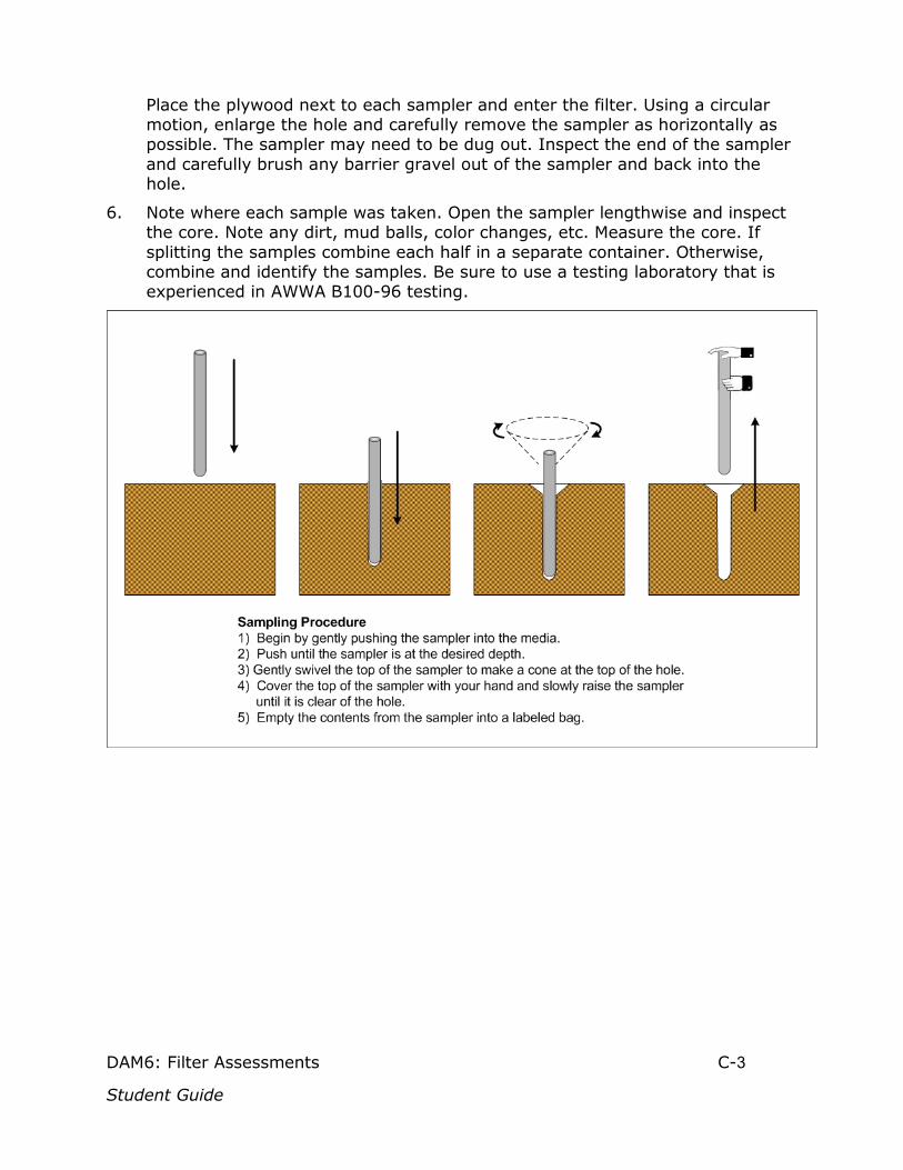
DAM6: Filter Assessments C-3
Student Guide
Place the plywood next to each sampler and enter the filter. Using a circular motion, enlarge the hole and carefully remove the sampler as horizontally as possible. The sampler may need to be dug out. Inspect the end of the sampler and carefully brush any barrier gravel out of the sampler and back into the hole.
6. Note where each sample was taken. Open the sampler lengthwise and inspect the core. Note any dirt, mud balls, color changes, etc. Measure the core. If splitting the samples combine each half in a separate container. Otherwise, combine and identify the samples. Be sure to use a testing laboratory that is experienced in AWWA B100-96 testing.
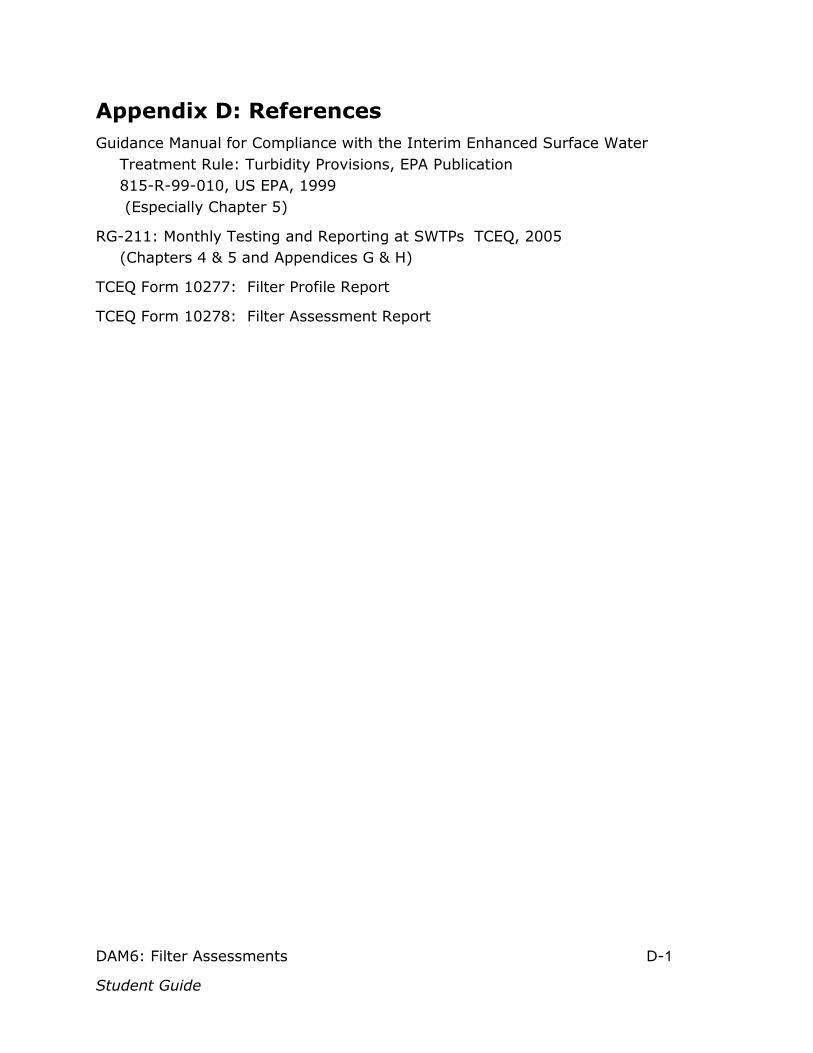
DAM6: Filter Assessments D-1
Student Guide
Appendix D: References Guidance Manual for Compliance with the Interim Enhanced Surface Water
Treatment Rule: Turbidity Provisions, EPA Publication 815-R-99-010, US EPA, 1999 (Especially Chapter 5)
RG-211: Monthly Testing and Reporting at SWTPs TCEQ, 2005 (Chapters 4 & 5 and Appendices G & H)
TCEQ Form 10277: Filter Profile Report
TCEQ Form 10278: Filter Assessment Report

DAM6: Filter Assessments
Student Guide E-1
Appendix E: Definitions and Acronyms The following table is provided to describe the terms used in this document as used in the context of this document. No attempt is made to provide precise technical or official definitions. Where appropriate, the reader is referred to the section or subsection of the Student Text for a description not practical to include here.
Section Term or (Subsection) Definition or Reference Abbreviation in the
Student Text
*.csv A file extension indicating a comma separated value file 2.1.3
1720E The Hach model number for a specific on-line turbidimeter
2100N The Hach model number for a specific benchtop turbidimeter
Air Releases In this application, the term is used to describe the air 3.1.1 passing upward through the filter media from the underdrain or the media bed itself.
Application The rate that settled water is applied to each square foot Rate (ft2) of filter surface area
Baseline Filter See the Student Text 2.2.1 Performance
Bed The number of inches a media bed is expanded divided by 4.5.2 Expansion the unexpanded depth of the bed
Backwash The rate that treat water is applied to each square foot (ft2) 4.5.1 Rate of filter surface area for backwashing
Backwash The upward velocity of the backwash water: the backwash 4.5.1 Rise Rate flow rate in gpm/ft2 times 12 inches per foot divided by
7.48 gallons/ft3
Backwash The total quantity of backwash water used for one filter 2.3.3.2 Volume backwash, normally in 1,000s of gallons.
Bench Sheets A hand written or printed record kept by the operators to 2.1.1 record production and performance data. (Also Daily Logs or Operator Logs)
CFE Combined Filter Effluent 2.1.4
CL17 A specific on-line chlorine residual analyzer by Hach
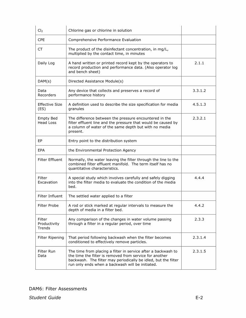
DAM6: Filter Assessments
Student Guide E-2
Cl2 Chlorine gas or chlorine in solution
CPE Comprehensive Performance Evaluation
CT The product of the disinfectant concentration, in mg/L, multiplied by the contact time, in minutes
Daily Log A hand written or printed record kept by the operators to record production and performance data. (Also operator log and bench sheet)
2.1.1
DAM(s) Directed Assistance Module(s)
Data Recorders
Any device that collects and preserves a record of performance history
3.3.1.2
Effective Size (ES)
A definition used to describe the size specification for media granules
4.5.1.3
Empty Bed Head Loss
The difference between the pressure encountered in the filter effluent line and the pressure that would be caused by a column of water of the same depth but with no media present.
2.3.2.1
EP Entry point to the distribution system
EPA the Environmental Protection Agency
Filter Effluent Normally, the water leaving the filter through the line to the combined filter effluent manifold. The term itself has no quantitative characteristics.
Filter Excavation
A special study which involves carefully and safely digging into the filter media to evaluate the condition of the media bed.
4.4.4
Filter Influent The settled water applied to a filter
Filter Probe A rod or stick marked at regular intervals to measure the depth of media in a filter bed.
4.4.2
Filter Productivity Trends
Any comparison of the changes in water volume passing through a filter in a regular period, over time
2.3.3
Filter Ripening That period following backwash when the filter becomes conditioned to effectively remove particles.
2.3.1.4
Filter Run Data
The time from placing a filter in service after a backwash to the time the filter is removed from service for another backwash. The filter may periodically be idled, but the filter run only ends when a backwash will be initiated.
2.3.1.5

DAM6: Filter Assessments
Student Guide E-3
Filter Run Head Loss
The difference between the empty bed head loss at the beginning of a filter run and the head loss encountered at the end of the filter run.
2.3.2.2
Floc Retention Analysis
A special study which involves applying water or a dilute acid to remove matter collected on the media during a filter run.
4.5.6
ft2 Square-feet or square-foot
ft3 Cubic feet (Used to indicate the volume of a solid, liquid, or gas) One ft3 is normally said to be equal to 7.48 gallons.
gpm Gallons per minute: the number of gallons in a flow volume divided by the number of minutes it takes to obtain that volume
gpm/ft2 Gallons-per-minute divided by the area through which the volume passes in square feet
Head Loss Trends
See the Student Text 2.2.3
Historical Performance
See the Student Text 2.3.1.1
Hook Gauge A device used to measure the rise rate of backwash water or the filtration rate of water applied to a filter
4.2.1
Idealized Turbidity Profile
See the student text 2.3.1.4
IFE Individual filter effluent
IFE Turbidity Profiles
2.3.1
Manual Data Assembly
See the student text 2.2.2
mCPE Mandatory Comprehensive Performance Evaluation
Media Excavations
See the Filter Excavations 4.4.4
mg/L Milligrams per liter
MGD Millions of gallons per day
Mn Manganese

DAM6: Filter Assessments
Student Guide E-4
Momentum The tendency of an object to remain in motion relative to another object
4.3.1
Mounds and Depressions
See the Student Text 3.1.5.3
Mudballs 3.1.3
NH3 Ammonia
No. Number
Normalized Net Yield
2.3.3.2
NTU Nephelometric turbidity units: a measure the reflectivity of the particles in water
O&M Operations and maintenance
Operator Logs A hand written or printed record kept by the operators to record production and performance data. (Also Daily Logs or, Bench Sheets)
2.1.1
Phases of Operation
See the Student Text 1.2.2.1
Percent Net Yield
See the Student Text 2.3.3.3
Percentage of Turbidity Removal
See the Student Text 2.3.1.7
pH A measure of hydrogen ion concentration in a solution.
Pipe Weir See the Student Text 4.3.2
Post-Backwash Turbidity Spike
The turbidity profile of a filter after it has been returned to service following a backwash.
2.3.1.6
Retraction An anomaly where the filter media draws away from the wall of the filter.
3.1.5.1
Ripening See Filter Ripening 2.3.1.4
Rise Rate The rate at which backwash water would rise in the filter box if all water were retained in the filter.
4.5.1

DAM6: Filter Assessments
Student Guide E-5
Routine Data Analyses
See the Student Text 2
Routine Visual Observations
See the Student Text 3.1
Routinely Collected Data
See the Student Text 2.1
SCADA Supervisory Control and Data Acquisition 2.1.3
SCADA Records
Electronic or printed reports of process control and reporting data collected and retained by the SCADA system
2.1.3
SDWA Safe Drinking Water Act
Sieve Analysis See the Student Text 4.5.1
SOP Standard Operating Procedure
Special Studies
The implementation of evaluation and test procedures not considered routine.
4
Surface Accumulations
Matter retained on the surface of the filter bed and not passing into the depth of the media
3.1.5.2
(SWMORs) Surface Water Monthly Operating Reports (See the Student Text and RG211)
2.1.4
SWTR Surface Water Treatment Rule
Term or Abbreviation Definition or Reference
Section (Subsection)
in the Student Text
TCEQ Texas Commission on Environmental Quality
TOP Texas Optimization Program
Turbidimeters Electronic test and/or monitoring devices used to measure the reflectivity of the particles in water (normally read in Nephelometric turbidity units or NTU).
3.3.1.1
Turbidity Profiles
A record of turbidity measured at regular intervals 2.3.1
Uniformity Coefficient (UC)
See the Student Text 4.5.1.3

DAM6: Filter Assessments
Student Guide E-6
Unit Comparisons
See the Student Text 2.3.1.2
Unit Filter Run Volume
See the Student Text 2.3.3.1

DAM6: Filter Assessments
Student Guide E-7
DAM 6. Evaluation Form
(to be completed by plant staff who participated in the training activities)
Training location: Date:
Instructor Name:
Strongly Agree Agree No Opinion Disagree Strongly Disagree
1. The agenda for this workshop accurately described the information being covered.
2. The information presented during the workshop was too technical or was too hard.
3. The information presented during the workshop was not technical enough.
4. The workshop covered too much information or the trainer went too fast.
5. The workshop covered too little information or the trainer went too slow.
6. The monitoring strategy developed during the workshop is useful.
7. The information on the Process Monitoring Form is understandable.
8. The training is exactly what we needed.
9. The training is valuable and will help us improve plant performance.
10. Our water system would be willing pay for this kind of training.
Questionnaire continues on the back

DAM6: Filter Assessments
Student Guide E-8
EVALUATION FORM, CONTINUED
Specific Suggestions: What could we change in the agenda to improve it?
What did we not explain well enough for you to understand?
What areas did we spend too much time on?
What areas did we spend too little time on?
What are some other issues where you feel more training is needed?
What other comments or suggestions do you have?
DAM6: Filter Assessments
Student Guide E-9
Inside back cover
Revision table
Date Action Comment
August 24, 2019 Revised Revised to meet TCEQ accessibility standards

Thanks for participating in this Directed Assistance Module (DAM)