Induction

In 1830-1831, Joseph Henry & Michael Faraday discovered electromagnetic

induction. Induction requires time varying magnetic fields and is the subject of another

of Maxwell's Equations.

Modifying Ampere's Law to include the possibility of time varying electric fields gives

the fourth Maxwell's Equations.

Faraday's Law

Changing magnetic flux in a conducting loop produces an induced emf in the

conducting loop that depends on the time rate of change of the magnetic flux.

For the conducting loop, find the magnetic flux and its time rate of change:

)(θBACosAB =⋅=Φ ⊥

SI unit of ΦΦΦΦ is the Weber 1W = 1Tm2

Three ways by which the flux may vary in time are:

1) Amount of magnetic field changes

2) Loop cross-section area changes

3) Changes in the relative orientation of ntoB ˆ__

Method 3) is used in an electric generator with input mechanical energy.

Effectively the opposite of an electric motor, the changing orientation of the loop n̂

relative to B results in a generated emf via induction in the conducting loop.

For a changing magnetic flux, the induced emf in the conducting loop is:

tEmf

Δ

ΔΦ−=

In an AC generator, if the loop rotates at a constant angular velocity ω :

( ) )()( tSinBAtCost

BAt

Emf ωωω =ΔΔ

−=ΔΔΦ

−=

Using a coil with N tightly packed loops,

)()( 0 tSinEtSinNBAEmf ωωω ==

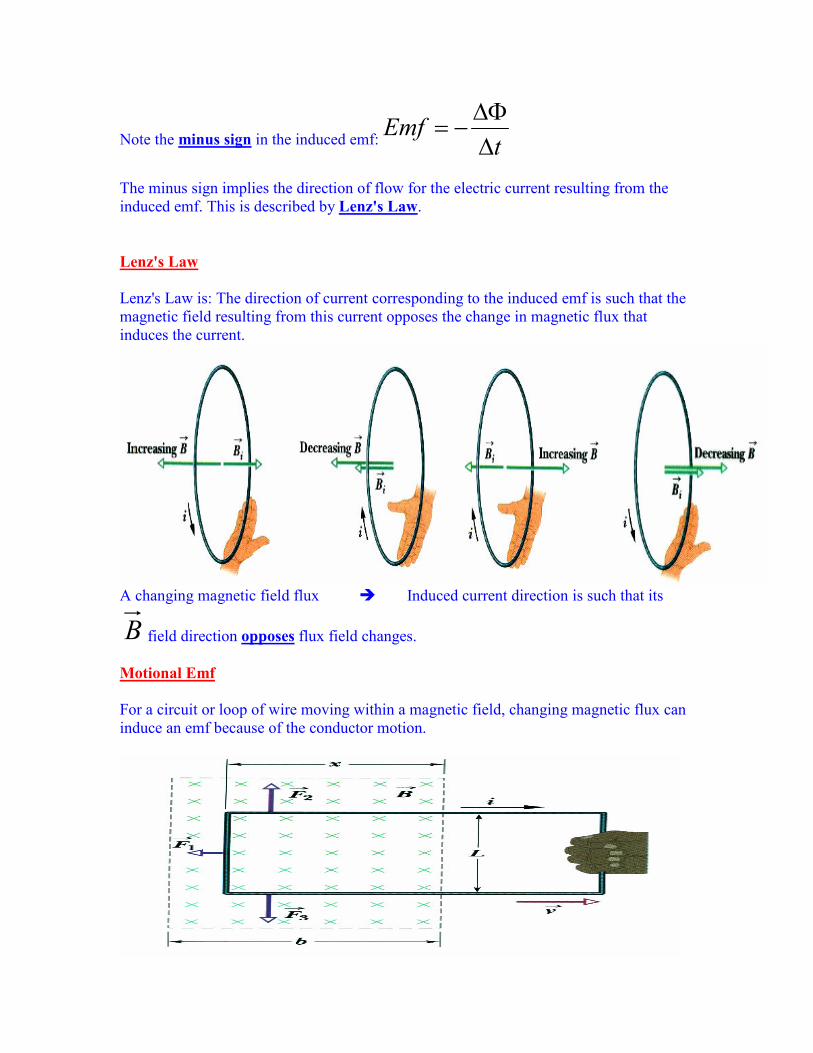
Note the minus sign in the induced emf: tEmf

ΔΔΦ

−=

The minus sign implies the direction of flow for the electric current resulting from the

induced emf. This is described by Lenz's Law.

Lenz's Law

Lenz's Law is: The direction of current corresponding to the induced emf is such that the

magnetic field resulting from this current opposes the change in magnetic flux that

induces the current.

A changing magnetic field flux � Induced current direction is such that its

B field direction opposes flux field changes.

Motional Emf

For a circuit or loop of wire moving within a magnetic field, changing magnetic flux can

induce an emf because of the conductor motion.

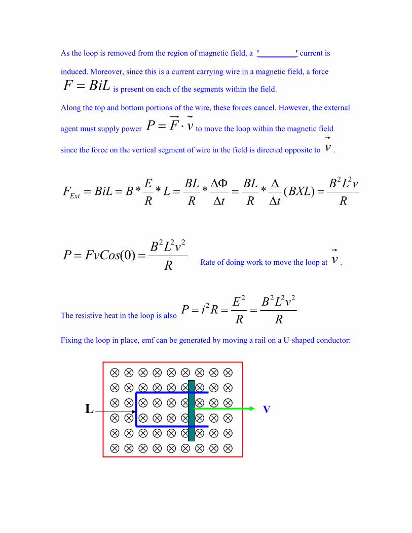
As the loop is removed from the region of magnetic field, a '_________' current is

induced. Moreover, since this is a current carrying wire in a magnetic field, a force

BiLF = is present on each of the segments within the field.

Along the top and bottom portions of the wire, these forces cancel. However, the external

agent must supply power vFP ⋅= to move the loop within the magnetic field

since the force on the vertical segment of wire in the field is directed opposite to v .

R

vLBBXL

tR

BL

tR

BLL

R

EBBiLFExt

22

)(**** =ΔΔ

=ΔΔΦ

===

R

vLBFvCosP

222

)0( == Rate of doing work to move the loop at v .

The resistive heat in the loop is also R

vLB

R

ERiP

22222 ===

Fixing the loop in place, emf can be generated by moving a rail on a U-shaped conductor:

L V

⊗ ⊗ ⊗ ⊗ ⊗ ⊗ ⊗ ⊗ ⊗⊗ ⊗ ⊗ ⊗ ⊗ ⊗ ⊗ ⊗ ⊗⊗ ⊗ ⊗ ⊗ ⊗ ⊗ ⊗ ⊗ ⊗⊗ ⊗ ⊗ ⊗ ⊗ ⊗ ⊗ ⊗ ⊗⊗ ⊗ ⊗ ⊗ ⊗ ⊗ ⊗ ⊗ ⊗⊗ ⊗ ⊗ ⊗ ⊗ ⊗ ⊗ ⊗ ⊗

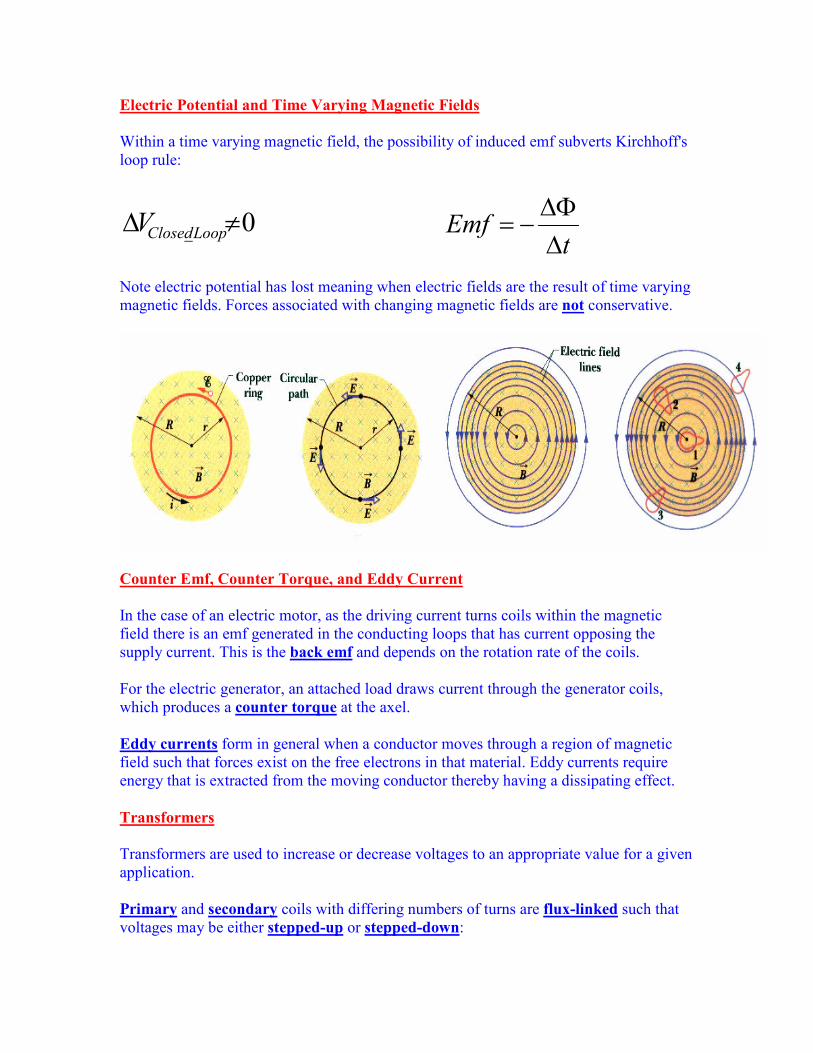
Electric Potential and Time Varying Magnetic Fields

Within a time varying magnetic field, the possibility of induced emf subverts Kirchhoff's

loop rule:

dt

dEmfV LoopClosed

Φ−=≠Δ 0_ t

EmfΔ

ΔΦ−=

Note electric potential has lost meaning when electric fields are the result of time varying

magnetic fields. Forces associated with changing magnetic fields are not conservative.

Counter Emf, Counter Torque, and Eddy Current

In the case of an electric motor, as the driving current turns coils within the magnetic

field there is an emf generated in the conducting loops that has current opposing the

supply current. This is the back emf and depends on the rotation rate of the coils.

For the electric generator, an attached load draws current through the generator coils,

which produces a counter torque at the axel.

Eddy currents form in general when a conductor moves through a region of magnetic

field such that forces exist on the free electrons in that material. Eddy currents require

energy that is extracted from the moving conductor thereby having a dissipating effect.

Transformers

Transformers are used to increase or decrease voltages to an appropriate value for a given

application.

Primary and secondary coils with differing numbers of turns are flux-linked such that

voltages may be either stepped-up or stepped-down:

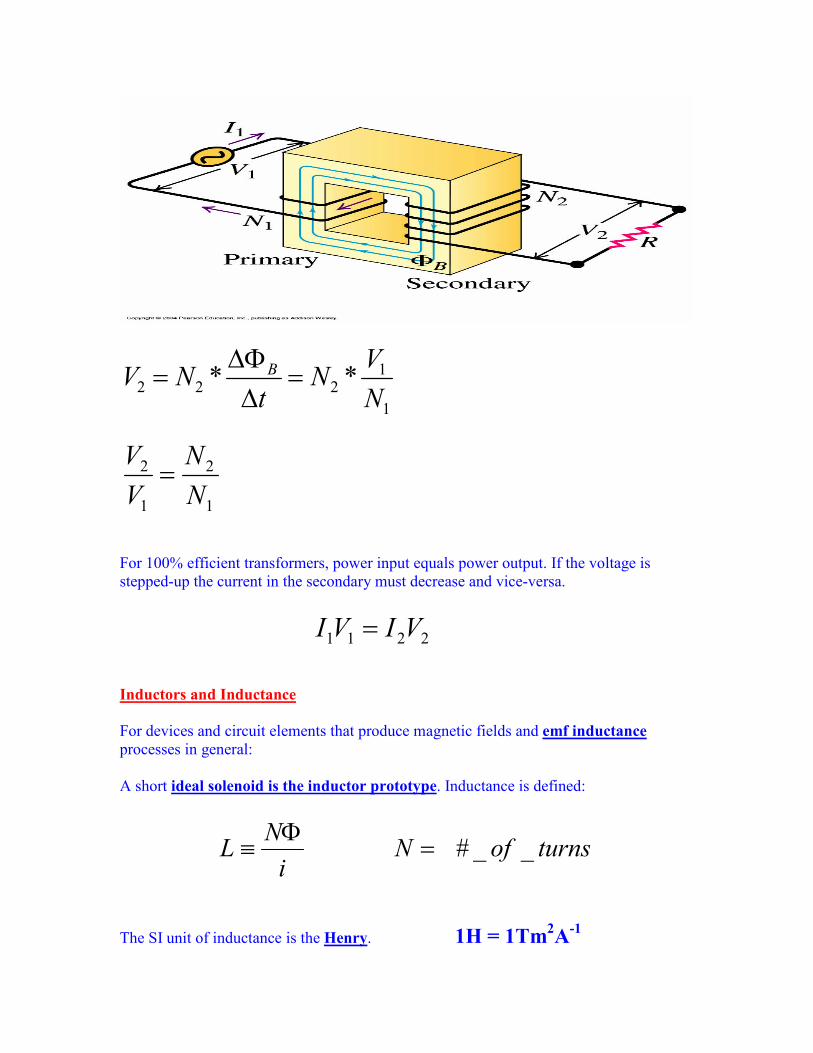
1

1222 **N

VN

tNV B =

ΔΔΦ

=

1

2

1

2

N

N

V

V=

For 100% efficient transformers, power input equals power output. If the voltage is

stepped-up the current in the secondary must decrease and vice-versa.

2211 VIVI =

Inductors and Inductance

For devices and circuit elements that produce magnetic fields and emf inductance

processes in general:

A short ideal solenoid is the inductor prototype. Inductance is defined:

turnsofNi

NL __#=

Φ≡

The SI unit of inductance is the Henry. 1H = 1Tm2A-1

ΦN is the flux linkage. Inductance is: flux linkage per unit current.

Increased inductance may be achieved by increasing the number of turns per unit length

on the inductor.

E.g., Ideal Solenoid:

niB 0µ= n here is turns per unit solenoid length.

nAnli

niANBA

i

N

i

NL 0

0* µµ

===Φ

≡

)(2

0 GeometryflAnL == µ

AnlL 2

0µ= In units of henry/meter.

Note the units of permeability are, therefore, henry/meter and recall from capacitance

that the units of permitivity are farad/meter.

Self Induction

Given an inductor and given a changing current tiΔ

Δwithin its coils, this changing

current produces a changing B in the inductor, and therefore a self-induced emf.

The induced current direction is such that the induced magnetic field produced from

this current counters whatever change is occurring in the inductor flux.

t

iL

t

ilAnni

tNABA

tN

tNE

Δ

Δ−=

Δ

Δ−=

Δ

Δ−=

Δ

Δ−=

Δ

ΔΦ−= 2

00)( µµ

t

iLE

ΔΔ

−=

For steady currents, the induced emf is zero.

For an ideal inductor, the resistance of the wire material is negligible, and the voltage

across the inductor is the self-induced emf.

If current is steady the inductor behaves as a short with zero voltage drop.

In practice, real inductors may be modeled by the series combination of an inductor

resistance outside the region of changing magnetic fields plus an ideal inductor.

Mutual Inductance

Consider interactions between two inductors in 'nearby' proximity. As current in inductor

#1 changes in time, this produces a changing magnetic field in inductor #1 and therefore

a changing flux in nearby inductor #2. Changing flux in inductor #2 produces an emf in

inductor #2. This is mutual inductance.

Similarly, any changes in inductor #2 current will induce an emf in inductor #1.

The mutual inductance of inductor 2 with respect to inductor 1 is:

1

21221

i

NM

Φ=

As with self-inductance, M is characterized by geometry.

212

21

21 Et

Nt

iM −=

ΔΔΦ

=ΔΔ

t

iME

ΔΔ

−= 1212 Induced emf in inductor #2 from a changing current in #1.

Similarly t

iME

Δ

Δ−= 2

121

Usually a small-unwanted effect in circuitry, mutual inductance is the way step-up / step-

down transformers operate.

Magnetic Field Energy Density

The energy stored in an inductor is magnetic energy.

Inductor magnetic field energy density is A

i

l

LlALi

V

Uu B

2/

2

1 22 ===

Which, given An

lL 2

0µ=, reduces to

22

02

1inu µ=

Using niB 0µ= gives: 0

2

2µB

u = Energy density of magnetic field.

RL Circuits

In an approach analogous to what was done with charging/discharging in an RC circuit,

the current response in an RL circuit may be evaluated starting from Kirchhoff's rule:

Recall the RC circuit results as follows: 0=−−

C

QiRE

Charging )1( τt

eCEQ−

−= RC=τ

Discharging τt

eQQ−

= 0

In an RL circuit, the inductor initially appears as open and eventually t���� ∞∞∞∞ as a short.

0=ΔΔ

−−t

iLiRE

Taking iQ → & L

R

RC→

1

)1()( τt

eR

Eti

−−=

.__ ConstTimeInductive

R

L==τ

The voltage on the inductor is a maximum to start and exponentially tends to zero:

ττ

τ

tt

L EeeR

LE

t

iLV

−−==

ΔΔ

−=

Using Kirchhoff's loop rule, the resistor voltage is therefore:

)1( ττtt

LR eEEeEVEV−−

−=−=−=

Zero to start and asymptotically tending to E as the inductor appears to short.

Removing the circuit emf,

ττtt

eR

Eeiti

−−== 0)(

LC Oscillators

Directly analogous to the mass-spring oscillating mechanical system, the electronic

counterpart is that of an inductor-capacitor oscillating circuit.

Oscillations are electromagnetic oscillations of capacitor electric fields and inductor

magnetic fields.

The circuit has all the properties of an oscillating system including a resonance driving

frequency, in this case LC/1=ω vs. mk /=ω for the mechanical system.

A correspondence of 1−→→ kCandmL is made.

Solutions to the differential equations describing the capacitor charge )(tq may be

extracted from the mechanical system solutions by making the appropriate variable

substitutions into those results.

Simple Harmonic Oscillation

A capacitor charge that is periodic or repeats in regular time intervals, and is a sinusoidal

or co-sinusoidal function of time is referred to as simple harmonic in time.

)()( φω += tQCostq

Q is the amplitude and is the maximum +/- capacitor charge.

ωωωω is the angular frequency of the oscillator and related to the frequency by ω=2πω=2πω=2πω=2πf

φφφφ is a phase factor or phase angle in units of radians.

f is the frequency or number of oscillations per second. Units of f are Hertz, Hz.

LC Circuit ⇔ Mass-Spring Analogy

Newton's 2nd Law for the mass-spring oscillator is:

kxma −=

)()( tCosxtx m ω=

)()( 2 tCosxta m ωω−=

Substituting: 0)()(2 =+− tCoskxtCosxm mm ωωω

This equation is true iff mk /=ω

From the circuit energies, and conservation of energy without resistive damping,

electromagnetic oscillations take place as follows:

._2

1

2

1 22 constEnergyTotal

C

qLiE ==+=

t

q

C

q

t

iLiE

ΔΔ

+ΔΔ

== 0&

01

=+ΔΔ

ΔΔ

qLCt

q

t Compared To 0=+

ΔΔ

ΔΔ

xm

k

t

x

t

Using 1& −→→ kCmL , then xq → is also appropriate.

For the circuit oscillator, 'kinetic' and 'potential' energies are the energies within the

inductor and capacitor respectively. The capacitor is spring like in its electric potential

energy, inductance mass like, and current a 'velocity' term.

)()( φω += tQCostq LC/1=ω

)()()( φωφωω +−=+−=ΔΔ

= tISintQSint

qti

amplitudecurrentQI _== ω

Let 0=φ and 'extend the mass', i.e., charge the capacitor to its full charge:

Qtq == )0( )()( tQCostq ω=

)()( tISinti ω−= 0)0( ==ti

The system oscillates as shown:

Initially:

CQ

tQCosC

qC

tUE 2)]([

2

1

2

1)(

222 === ω

0)]([*2

1

2

1)( 22 =−== tISinLLitUB ω

At ωπ24

==Tt

0)]([2

1

2

1)( 22 === tQCos

Cq

CtUE ω

222

2

1)]([*

2

1

2

1)( LItISinLLitUB =−== ω

Etc., the system evolves periodically transferring energy between the capacitor electric

field and the inductor magnetic field as shown.

Both 'kinetic' and 'potential' energy peaks occur twice over the course of 1 period [T].

Since LC/1=ω the total energy at all times is:

2222

2

1)}()({

2

1)()( Q

CtCostSinQ

CtUtUE EB =+++=+= φωφω

The electromagnetic energy is a constant provided resistive damping is absent.

RLC Circuits, Damped Harmonic Oscillations

Most non-driven oscillating systems will come to rest after a finite amount of time due to

dissipative losses. In the RLC circuit, the resistor damps the LC oscillations causing

exponentially decaying oscillation amplitude.

The general solution is a linear combination of the two possibilities:

}{)(*)(*)(

20

220

2 ttt BeAeetqωγωγγ −−−− +=

Three cases exist depending on whether γγγγ2222 < ω < ω < ω < ω00002222 , γ , γ , γ , γ2222 > ω > ω > ω > ω0000

2 2 2 2 , or γ γ γ γ2222 = ω = ω = ω = ω0000

2222

Case 1 Underdamped Solution:

γγγγ2222 < ω < ω < ω < ω00002 2 2 2 � C

LR 2<

}{)(*)(*)( 22

022

0 titit BeAeetqγωγωγ −−−− +=

})()()(){()( 22

0

22

0 tiSinBAtCosBAetq t γωγωγ −−+−+= −

)}'(')'('{)( tSinBtCosAetq t ωωγ += −

With initial conditions q(0) = Q and i(0) = 0,

A' = Q

B'ωωωω' - A'γγγγ = 0 B' = = = = A'γγγγ/ωωωω' = Q {γ/ωγ/ωγ/ωγ/ω'}

)}'('

)'({)( tSintCosQetq t ωωγ

ωγ += −

Wishing to write something like:

)}'({'

)( 0 φωωω γ += − tCoseQtq t

We find the phase angle φ must be: '

1

ωγ

φ −−= Tan

Proving this requires:

)'('

)'()}'({'

0 tSintCostCos ωωγ

ωφωωω

+=+

From trigonometry the LHS is

)}()'()()'({'

0 φωφωωω

SintSinCostCos −

}'

{)( 1

ωγ

φ −= TanCosCos

The reference triangle is: 22 'ωγ +

γγγγ

ωωωω'

22

0' γωω −= � 0

22 ' ωωγ =+

0

')( ωωφ =Cos

� 0

)( ωγφ −=Sin

From which,

)'('

)'()}'({'

0 tSintCostCos ωωγ

ωφωωω

+=+

φφφφ

)}'({'

)( 0 φωωω γ += − tCoseQtq t

'

1

ωγ

φ −−= Tan

The oscillation amplitude is decaying exponentially in time.

Case 2 Critically Damped Solution:

γγγγ2222 = ω = ω = ω = ω00002222 � C

LR 2=

In this case ωωωω' is identically zero and we can evaluate the limiting form of:

)}'('

)'({)( tSintCosQetq t ωωγ

ωγ += −

As ωωωω' ���� 0.

)]}'('

)'([{0'

tSintCosQeLim t ωωγ

ωγ

ω+−

>−

The cosine term goes to 1 in the limit and the sine term is:

tt

tSintLimtSinLim γ

ωω

γωωγ

ωω==

>−>−}

'

)'(*{)}'(

'{

0'0'

}1{)( tQetq t γγ += −

The circuit damps to equilibrium as quickly as is possible without oscillation about the

equilibrium point.

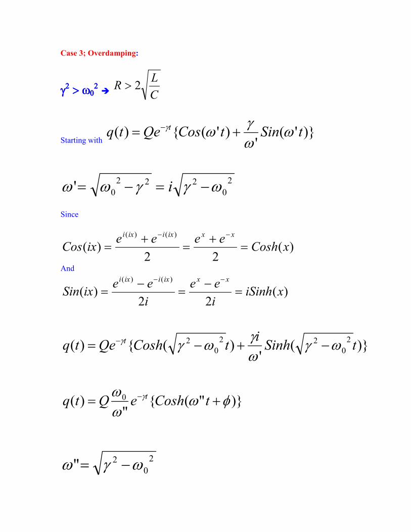
Case 3; Overdamping:

γγγγ2222 > ω > ω > ω > ω00002222 � C

LR 2>

Starting with )}'(

')'({)( tSintCosQetq t ω

ωγ

ωγ += −

2

0

222

0' ωγγωω −=−= i

Since

)(22

)()()(

xCosheeee

ixCosxxixiixi

=+

=+

=−−

And

)(22

)()()(

xiSinhi

ee

i

eeixSin

xxixiixi

=−

=−

=−−

)}('

)({)(2

0

22

0

2 tSinhi

tCoshQetq t ωγωγ

ωγγ −+−= −

)}"({"

)( 0 φωωω γ += − tCosheQtq t

2

0

2" ωγω −=

Alternating Current and AC Circuits

For a sinusoidal oscillating voltage, the currents in a circuit will be alternating current.

Since any input signal may be Fourier analyzed into a series summation of sine and

cosine inputs, the response of a circuit to a general AC signal will be important.

Depending on the combination of circuit elements R, L, and/or C, the driving emf

and circuit current will in general be out of phase with each other.

)( tSinEE dm ω= )( φω −= tISini d

Phasor projections along the vertical ����current / voltage at time = t

Resistive Load

For the above emf / resistor only circuit:

0=− RvE � )()( tSinVtSinEv dRdmR ωω ==

)()( tSinItSinR

Vi dRd

RR ωω ==

� RIV RR =

Current and voltage are in phase.

Capacitive Load

Using the AC emf with a capacitor:

)()( tSinCVCvqtSinVv dCCCdCC ωω ===

)( tCosCVt

qi ddC

CC ωω=

ΔΔ

=

Defining the capacitive reactance CX

d

C ω1

=

)2

(π

ω += tSinX

Vi d

C

CC

� Current leads voltage by 90 degrees

Then since )( φω −= tSinIi dCC � 2

πφ −=

And CCC XIV =

Inductive Load

AC source and inductor only:

t

iLtSinVv dLL Δ

Δ== )(ω

Defining the Inductive reactance as LX dL ω=

)2

(π

ω −= tSinX

Vi d

L

LL

� Current lags voltage by 90 degrees

Then since )( φω −= tSinIi dLL � 2

πφ +=

And LLL XIV =

Series RLC Circuits

In general: )( tSinEE dm ω=

)( φω −= tISini d

φandI to be determined.

The Phasor algebra looks like:

From Kirchhoff's Rule, 0=−−− CLRm VVVE

The current and RV are in phase and the phase angle between current and emf is φ

.

222222)()( CLCLRm XXIRIVVVE −+=−+=

2 2

22 )( CL

m

XXR

EI

−+=

The impedance is:

22 )( CL XXRZ −+=

22 )1

(C

LR

E

ZE

I

d

d

mm

ωω −+

==

From the figure, the phase angle φ

is:

R

XX

V

VVTan CL

R

CL −=

−=)(φ

Three cases are as follows:

1) Inductive circuit 0>φ

Voltage leads current

2) Capacitive circuit 0<φ

Voltage lags current

3) Resonance 0=φ

Voltage and current are in phase.

Starting the emf at low frequency and scanning to higher values of dωwill produce an

observable phase shift in i relative to E as the circuit moves from a capacitive circuit

to an inductive circuit across the resonance point at LCd

1=ω

Resonance

Driving an RLC circuit at resonance condition produces output current and voltage

amplitudes that are maximal. The condition for resonance is:

0ωω =Driving 22 )1

(C

LR

V

Z

VI rmsrmsrms

ωω −+

==

22 )1

(C

LR

R

V

VAGain

in

outv

ωω −+

===

Notice as the damping R is reduced the resonant amplitude peaks become larger and

have narrower half-width. The series RLC is a useful bandwidth filter circuit near the

resonance frequency.

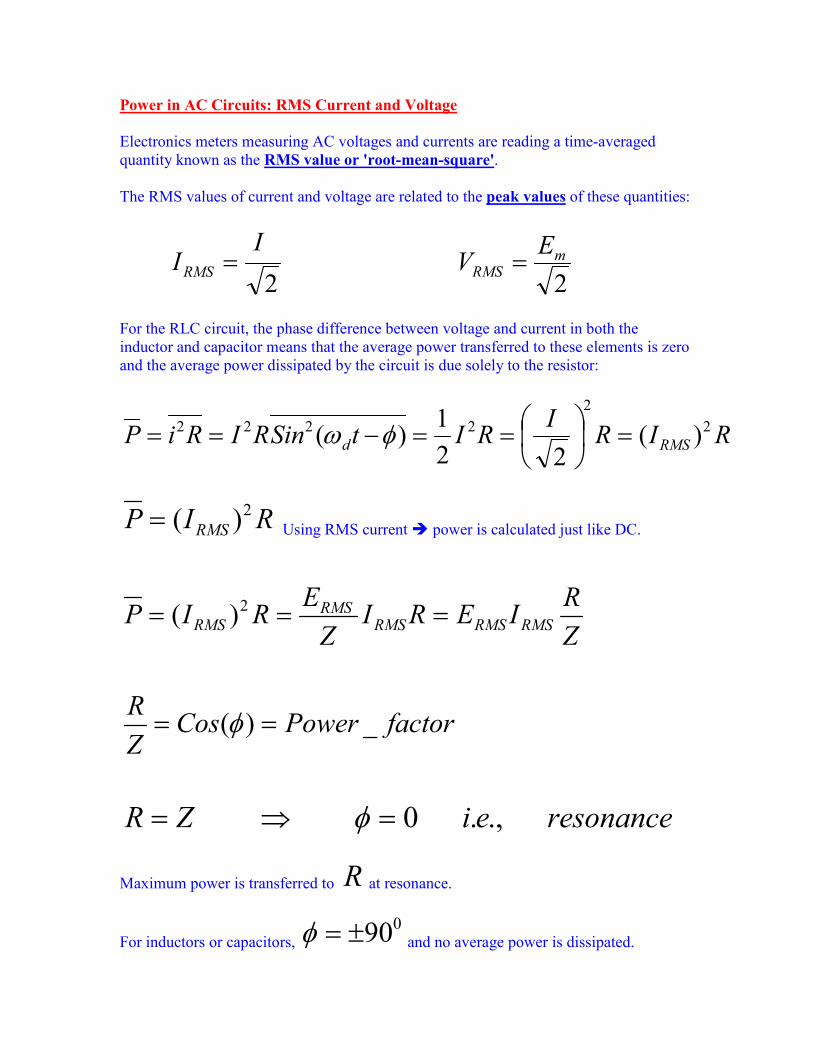
Power in AC Circuits: RMS Current and Voltage

Electronics meters measuring AC voltages and currents are reading a time-averaged

quantity known as the RMS value or 'root-mean-square'.

The RMS values of current and voltage are related to the peak values of these quantities:

2

IIRMS =

2

mRMS

EV =

For the RLC circuit, the phase difference between voltage and current in both the

inductor and capacitor means that the average power transferred to these elements is zero

and the average power dissipated by the circuit is due solely to the resistor:

RIRI

RItSinRIRiP RMSd

2

2

2222 )(22

1)( =

==−== φω

RIP RMS

2)(= Using RMS current � power is calculated just like DC.

Z

RIERI

Z

ERIP RMSRMSRMS

RMSRMS === 2)(

factorPowerCosZ

R_)( == φ

resonanceeiZR .,.0=⇒= φ

Maximum power is transferred to R at resonance.

For inductors or capacitors,

090±=φ and no average power is dissipated.

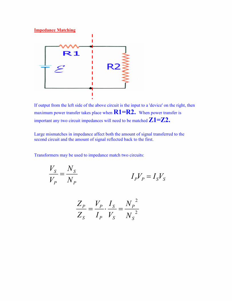
Impedance Matching

If output from the left side of the above circuit is the input to a 'device' on the right, then

maximum power transfer takes place when R1=R2. When power transfer is

important any two circuit impedances will need to be matched Z1=Z2.

Large mismatches in impedance affect both the amount of signal transferred to the

second circuit and the amount of signal reflected back to the first.

Transformers may be used to impedance match two circuits:

P

S

P

S

N

N

V

V=

SSPP VIVI =

2

2

S

P

S

S

P

P

S

P

N

N

V

I

I

V

Z

Z=⋅=