Embed Size (px)
Citation preview
Viet-An Nguyen, Jordan Boyd-Graber, and Stephen Altschul. Dirichlet Mixtures, the Dirichlet Process,and the Structure of Protein Space. Journal of Computational Biology, 2013, 48 pages.
@articleNguyen:Boyd-Graber:Altschul-2013,Title = Dirichlet Mixtures, the Dirichlet Process, and the Structure of Protein Space,Author = Viet-An Nguyen and Jordan Boyd-Graber and Stephen Altschul,Journal = Journal of Computational Biology,Year = 2013,Volume = 20,Number = 1,Url = http://umiacs.umd.edu/~jbg//docs/2013_dp_protein.pdf,
Links:
• Journal [http://online.liebertpub.com/doi/pdfplus/10.1089/cmb.2012.0244]
Downloaded from http://umiacs.umd.edu/~jbg/docs/2013_dp_protein.pdf
Contact Jordan Boyd-Graber ([email protected]) for questions about this paper.
1
Dirichlet Mixtures, the Dirichlet Process,
and the Structure of Protein Space
Viet-An Nguyen1, Jordan Boyd-Graber2 and Stephen F. Altschul3,∗
1 Department of Computer Science and UMIACS,
University of Maryland
College Park, MD 20740, United States
2 iSchool and UMIACS,
University of Maryland
College Park, MD 20740, United States
3 National Center for Biotechnology Information,
National Library of Medicine, National Institutes of Health,
Bethesda, MD 20894, United States
Tel.: +1 (301) 435-7803
Fax: +1 (301) 480-2288
September 29, 2012
∗Corresponding author
Abstract
The Dirichlet process is used to model probability distributions that are mix-
tures of an unknown number of components. Amino acid frequencies at homolo-
gous positions within related proteins have been fruitfully modeled by Dirichlet
mixtures, and we use the Dirichlet process to derive such mixtures with an un-
bounded number of components. This application of the method requires sev-
eral technical innovations to sample an unbounded number of Dirichlet mixture
components. The resulting Dirichlet mixtures model multiple alignment data
substantially better than do previously derived ones. They consist of over 500
components, in contrast to fewer than 40 previously, and provide a novel per-
spective on the structure of proteins. Individual protein positions should be seen
not as falling into one of several categories, but rather as arrayed near probability
ridges winding through amino-acid multinomial space.
2
1 Introduction
Given a multiple alignment of sequences from a particular protein family, how may one
estimate the amino acid frequencies found in related sequences at a specific alignment
position, and thereby construct scores for adding a new sequence to the alignment? An
elegant Bayesian approach to this problem was proposed in the 1990s by researchers
at UCSC (Brown et al., 1993; Sjolander et al., 1996). In brief, one may model a
particular position in a particular protein family by an unknown set of twenty amino
acid probabilities, a point in the multinomial space Ω20. Given a prior probability
density P over Ω20, Bayes’ theorem implies a posterior density P ′ after the observation
of several amino acids at the position in question. An estimate ~q for the amino acid
frequencies of the protein family at this position may then be derived by integrating P ′
over Ω20. Although the prior density P may be of arbitrary form, it is mathematically
convenient if P is assumed to be a Dirichlet distribution, or a mixture of M Dirichlet
distributions.
As the number of observed amino acids at a position grows, ~q converges to the
observed frequencies, no matter what the prior P is. However, given a small num-
ber of observations, ~q will in general be a better estimate of the actual probabilities
at the protein position if the prior P accurately describes the density over Ω20 char-
acteristic of real protein families. Discovering such a P given data is a problem of
posterior inference. One starts with a large “gold standard” dataset S of protein mul-
tiple alignments, which are assumed to be accurate. Each “column” from these multiple
alignments represents a particular position within a particular protein family, and it is
really these columns that may considered as constituting the dataset. One then seeks
the maximum-likelihood Dirichlet mixture (DM).
3
One immediate problems arises. The likelihood of S may in general be improved
by increasing the number of components of a DM until it roughly equals the number of
columns in S. Doing so, however, leads to the classic problem of overfitting the data,
which causes degraded predictions on new data. One solution is to apply the Minimum
Description Length principle (Grunwald, 2007), and seek instead to minimize the “total
description length” COMP(DM) + DL(S|θ) (Ye et al., 2011b).a The first term of this
expression is the “complexity” of the model DM consisting of all M -component DMs;
this can be understood as the log of the effective number of independent theories DM
contains (Grunwald, 2007). The second term is the negative log likelihood of S implied
by the maximum-likelihood θ drawn from DM . Although no feasible algorithm for
minimizing DL(S|θ) is known, approximations may be found using approaches based
on expectation maximization (Brown et al., 1993; Sjolander et al., 1996) or Gibbs
sampling (Ye et al., 2011b).
An alternative approach which never fixes M , but treats the number of compo-
nents as unknown, is possible using nonparametric Bayesian models. One such model
is the Dirichlet process (DP), which we apply to multiple alignment data. In brief, the
DP allows us to create a generalized prior probability density over the space of DMs
with an unlimited number of components. Posterior inference using a Gibbs sampling
algorithm moves naturally among mixture models with varying numbers of compo-
nents. The DP and its generalization, the Pitman-Yor distribution (Pitman and Yor,
1997), have been applied previously to Gaussian mixtures (Antoniak, 1974), mixtures
of multinomials (Hardisty et al., 2010), admixtures of multinomials (Teh et al., 2006),
time-dependent mixtures of multinomials (Beal et al., 2002), and mixtures of linear
models (Hannah et al., 2011), but not to Dirichlet mixtures. In describing probability
aOther validation approaches that are robust to overfitting include held-out perplexity (Blei et al.,2003) or extrinsic evaluation.
4
densities over ΩL, Dirichlet mixtures have much greater flexibility than do multinomial
mixtures. An individual multinomial component can model only probability concen-
trated at a specific location in ΩL, whereas a single Dirichlet component can model
densities that are arbitrarily concentrated around such a location, and even densities
with most of their mass near the boundaries of ΩL. The components of a Dirichlet
mixture may have probability densities of variable concentration. Thus, for example,
one component can favor positions with a fairly precise amino acid probability signa-
ture, whereas another can favor positions that contain hydrophobic amino acids, but
only one or a small subset of them.
When used to analyze the same dataset for which a previous study (Ye et al.,
2011b) yielded a 35-component DM, our DP-based Gibbs sampling algorithm yields
substantially improved solutions with over 500 components. Such large DMs may
be cumbersome for practical algorithms, but a specified trade-off between component
number and total description length can be used to select a DM with fewer components.
Of perhaps greater interest is the perspective on the structure of protein space
provided by DMs with many components. The DM formalism suggests, at first, the
metaphor of a small number of probability hills in Ω20, corresponding to different types
of protein positions—hydrophobic, aromatic, charged, etc. However, the density im-
plied by the many-component DMs we derive is dominated by a continuous probability
ridge winding through Ω20. This may provide a new perspective on how selective
pressures are felt at individual protein positions.
5
2 Methods
We here describe the mathematical underpinnings of our approach, providing a brief
review of standard material, and devoting more detailed discussion to less familiar or
novel methods.
2.1 Multinomial space
A multinomial probability distribution on an alphabet with L letters is a vector with
L positive components that sum to 1, and the space of all possible multinomials is
the simplex ΩL. Due to the constraints on the vector components, ΩL is finite and
has (L − 1) degrees of freedom. For example, Ω3 is the 2-dimensional equilateral
triangle, embedded in Euclidean 3-space, with vertices (1,0,0), (0,1,0) and (0,0,1). We
will be interested primarily in the standard amino acid alphabet, and therefore in the
19-dimensional space Ω20.
2.2 The Dirichlet distribution
For an alphabet of L letters, a Dirichlet distribution D is a probability density over
ΩL, parameterized by an L-dimensional vector ~α of positive real numbers greater than
zero; it is convenient to define α as∑L
j=1 αj. The density of D at ~x is given by
D(~x | ~α) ≡ Z
L∏
j=1
xαj−1j , (1)
where the normalizing scalar Z ≡ Γ(α)/∏L
j=1 Γ(αj) is chosen so that integrating D
over ΩL yields 1. The expectation or mean of ~x under the density of equation (1)
is the multinomial distribution parameterized by ~q ≡ ~α/α. It is frequently useful to
6
write D’s parameters in the form α~q, with α ∈ (0,∞), and ~q ∈ ΩL. When we use this
alternative parametrization for D, we write it as (~q, α). Intuitively, one may visualize
a Dirichlet distribution as a probability hill in ΩL, centered at ~q, and with greater α
corresponding to greater concentration of probability mass near ~q. For α near 0, the
“hill” in fact becomes a trough, with most probability concentrated near the boundaries
of ΩL. Thus, such Dirichlet distributions favor sparse multinomials where only a few
letters have non-negligible probability (Figure 1). Figure 1
2.3 Mixture models
Given a proposed set of observations, a theory may be thought of as assigning probabil-
ities to all possible datasets or outcomes. If a theory has a particular set of adjustable
parameters, we call the set of all such theories a model. More generally, we may wish
to consider multiple models, usually nested, characterized by different numbers or sets
of parameters.
Mixture models are a formalism frequently used to discover clustering patterns
in data. In a mixture model, all observations are associated with clusters, each of
which has a corresponding probabilistic mixture “component” that explains its data.
For example, multinomial mixture models are frequently used in text analysis (Lewis,
1998).
Multinomial mixtures have difficulty modeling many probability densities over ΩL,
because the L − 1 free parameters of an individual multinomial component can only
describe probability concentrated at a specific location ~q. In contrast, with the addi-
tion of the single extra parameter α, a Dirichlet component can describe probability
densities of arbitrary concentration around ~q, including, when α is small, densities that
favor sparse multinomials (Figure 1). This greatly enhanced flexibility allows a Dirich-
7
let mixture to model most real-world probability densities over ΩL much better than
can a multinomial mixture with many times as many components.
An M -component DM is a probability density over ΩL, defined as the weighted
sum of M Dirichlet distributions, called Dirichlet components. Such a mixture has
ML + M − 1 free parameters. Each of the M Dirichlet components contributes L
“Dirichlet parameters”. In addition, the weights ~w or “mixture parameters” are M
positive real numbers that sum to 1, only M −1 of which are independent. A DM may
be thought of as a superposition of M probability hills in ΩL, each with its particular
volume, center of mass and concentration.
2.4 The Dirichlet process
When seeking a theory for a set of data, a difficulty is that theories with more parame-
ters generally can explain the data better, but overfitting can result in poor predictions
on future data. One approach to this problem is the Minimum Description Length
principle (Grunwald, 2007), which explicitly favors theories drawn from mixture mod-
els with fewer components (Ye et al., 2011b). An alternative approach is provided by
the Dirichlet process (DP), which effectively subsumes in a single formalism mixture
models with an arbitrary number of components. A mathematically detailed descrip-
tion of the Dirichlet process (DP) can be found elsewhere (Antoniak, 1974; Pitman and
Yor, 1997; Muller and Quintana, 2004); here we will review only its essentials.
The DP generally is applied to problems where data are postulated to be well-
modeled as generated by a mixture of multiple instances (often called “atoms” but
here called “components”) of an underlying distribution of known parametric form. In
the DP formalism, every mixture consists of a countably infinite number of components,
each with its own weight and set of component parameters. In essence, a DP defines a
8
generalized probability distribution over this infinite-dimensional space of mixtures.
Two elements completely specify a DP:
1. A “base” probability distribution H over the space of component parameters.
For example, if the components are Gaussians on R with unit variance, H is a
specified distribution for their means.
2. A positive real parameter, which implicity defines a probability distribution on
component weights. This parameter is usually called α, but we will call it γ here
to avoid the potential confusion arising from the multiple distinct uses we make
of Dirichlet distributions. As we will see, the smaller γ, the greater the implied
concentration of weight in a few components.
Analysis using the DP is Bayesian. A DP is used to define a prior over mixture
distributions which, when combined with observed data, implies a posterior for the
weights and component parameters of these mixtures. A special feature of this infer-
ence is that, although all mixtures are assumed to have a countably infinite number of
components, only a finite number can ever explain a given set of data. The posterior
distribution thus differs from the prior only for finitely many components. Bayesian
analysis allows one to estimate the number of these components, as well as their asso-
ciated weights and component parameters.
2.5 The Chinese restaurant process
The “Chinese restaurant process” (CRP) (Ferguson, 1973) is closely related to the
Dirichlet process and is useful for understanding the properties of the DP, as well
as for posterior inference. The metaphor in the name refers to a restaurant with an
unbounded number of tables.
9
The Chinese restaurant is patronized by customers. Each customer represents an
i.i.d. draw from a distribution G drawn from a Dirichlet process DP (γ,H).b Each
customer sits at one of the tables, and when customers sit at the same table it means
they are associated with the same component, drawn from the base distribution H.
In our application, a customer represents a multiple-alignment column, and a table
represents a DM component, (~qk, αk).
Draws from the Dirichlet process are exchangeable (Aldous, 1985), so each customer
can be viewed as the “last” customer to enter the restaurant. When customers enter,
they choose to sit either at a new table or at one that is already occupied. This choice
is made randomly, but with each occupied table selected with probability proportional
to the number of people already seated there, and a new table selected with probability
proportional to the parameter γ. It is evident that smaller values for γ imply a greater
concentration of customers at a small number of tables.
The exchangeability of the Dirichlet process is important for Gibbs sampling in-
ference, because it allows us to condition one column’s component assignment on the
other columns’ assignments.
2.6 A base distribution for Dirichlet-component parameters
Specifying a DP for Dirichlet mixtures requires specifying a base distribution H over
the space of Dirichlet parameters. Rather than defining H on the standard Dirichlet
parameters ~α ∈ R+L, we find it more natural to define it on the alternative parameters
(~q, α). Specifically, we propose H ≡ (H1, H2), where H1 and H2 are independent
distributions for ~q and α.
bNote that the Chinese restaurant does not model a specific measure G; it only models draws fromG and integrates over all possible G. However, this representation is sufficient for our purposes. Fora constructive definition of the Dirichlet process, see (Sethuraman, 1994).
10
Because ~q ∈ Ω20, a natural base distributionH1 for ~q is itself Dirichlet. Furthermore,
because we seek a DM that describes protein columns, it is appropriate to choose H1’s
center of mass to be ~p, the “background” amino acid frequencies typical for proteins.
This leaves only the single concentration parameter, which we will call β. In short, we
propose choosing H1 to be the Dirichlet distribution with parameters (~p, β).
When specifying H2, the base distribution for α ∈ (0,∞), we will see that it is
convenient if we require H2 to have a long, uninformative tail. An exponential function
of the form H2 ≡ λe−λα, with λ small, serves the purpose, and the precise value of λ
will be irrelevant.
By choosing ~p as the center of mass for H1, and requiring H2 to have a long tail, the
base distribution H ≡ (H1, H2) we propose for Dirichlet-component parameters has, in
effect, only the one free parameter β, as results are insensitive to the choice of λ. This,
in conjunction with the parameter γ, completes our specification of a DP for Dirichlet
mixtures. We will discuss in the Results section the effects of different choices for β
and γ.
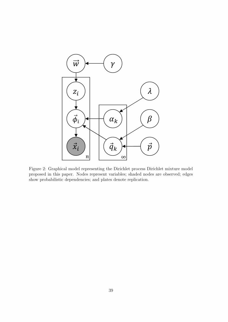
2.7 ModelFigure 2
To review, we posit the following generative process for observed data:
• We draw component k ∈ [1,∞) of the Dirichlet process from the base distribution;
this draw has two parts:
– the component’s mean ~qk is sampled from Dirichlet(~p, β);
– the component’s concentration αk is sampled from Exponential(λ), which is
equivalent to a Gamma distribution with shape = 1 and rate = λ.
11
• We draw weights ~w for all of the Dirichlet process components from GEM(γ).c
• For each column i ∈ [1, n]:
– We draw a component assignment zi from the distribution ~w;
– We draw a multinomial distribution ~φi over letters from Dirichlet(~qzi , αzi);
– We draw the letters of column i from Multinomial(~φi), resulting in the
observation vector ~xi, with associated letter count vector ~ci.
We assume that this process created the observed columns and use posterior inference,
described in the rest of the section, to uncover the latent variables that best explain
the observed data. The generative process may be expressed using the graphical model
in Figure 2.
At this point, we pause to recognize that our terminology has potential confusions.
Our model has three different uses of the word “Dirichlet”. One is a Dirichlet process,
and two are ordinary Dirichlet distributions:
• At the top level, a Dirichlet process gives us a countably infinite number of
components. This is a nonparametric Bayesian distribution over distributions.
• Each component k of the Dirichlet process is itself a Dirichlet distribution, param-
eterized by (~qk, αk). This is a finite distribution over Ω20. Columns are generated
from a multinomial drawn from this distribution.
• The mean of each component’s Dirichlet distribution is itself drawn from a Dirich-
let distribution parameterized by (~p, β).
cThe vector ~w is a point on the infinite simplex (Sethuraman, 1994) and GEM stands for Grif-fiths (Griffiths, 1980), Engen (Engen, 1975), and McCloskey (McCloskey, 1965). This, along with theseparate component draws, form a constructive “stick breaking” definition of the Dirichlet process.
12
2.8 MCMC inference for Dirichlet process Dirichlet mixtures
The Gibbs sampling algorithm for DMs described in (Ye et al., 2011b) assumed a fixed
number of components M . The algorithm alternated between a first stage, in which
the component assignments zi for columns were chosen by Gibbs sampling, conditioned
on the complete set of component parameters, and a second stage, in which each
component’s parameters were updated, using maximum-likelihood estimates based on
the columns associated with that component. Our approach here, although similar in
many ways, has a few key differences.
Like the previous approach, our Gibbs sampler forms a Markov chain over assign-
ments to components Z ≡ z1, z2, · · · , zn and component parameters (~q1, α1), (~q2, α2) . . . .
However, unlike the previous approach, the number of components is not fixed. Com-
ponents can be both lost and created, but only finitely many components are ever used
to describe a given dataset. Specifically, before being assigned stochastically to a new
component, by means of the latent variable zi, a column i is first removed from an
existing one, and if this component is left with no associated columns, it is abolished.
Then, for the column’s new assignment, it may choose among the existing components,
but it may also start a new one. Unlike in (Ye et al., 2011b), this sampling is con-
ditioned on the current component assignments of all other columns, rather than on
those assignments only from the previous round. During the algorithm’s second stage,
we sample component parameters, rather than update them by maximum-likelihood
estimation. There are various ways in which one may initialize the algorithm, but the
simple expedient of assigning all columns to a single component at the start does not
appear to cause any difficulties. We describe in greater detail below various technical
aspects of these modifications to the algorithm of (Ye et al., 2011b).
13
2.9 Sampling an existing or new component for a column
Our DP-sampling algorithm creates a Markov chain of component assignments and
component parameters. While sampling component assignments, we assume that the
Dirichlet parameters ~αk associated with an existing component k remain fixed. How-
ever, the number of columns nk associated with component k may change.
Gibbs sampling conditions a column’s assignment zi on the other columns’ assign-
ments and the component parameters. This is where the exchangeability of the Chinese
restaurant process (Section 2.5) is advantageous. Computing the conditional distribu-
tion is equivalent to removing column i from its current component and then assigning
it to an existing component or a completely new one. Assuming the observations ~xi of
column i contain ci total amino acids, with the amino acid counts given by the vector
~ci, the likelihood for an existing component k is proportional to
p(zi = k | Z−i, ~qk, αk, ~xi) ∝ nk ·Γ(αk)
Γ(αk + ci)
20∏
j=1
Γ(αkqk,j + ci,j)
Γ(αkqk,j)(2)
(Brown et al., 1993; Sjolander et al., 1996; Altschul et al., 2010; Ye et al., 2011b). Here,
Z−i denotes the set of component assignments for all columns except column i. In the
Chinese restaurant metaphor, this corresponds to sitting at an existing table.
In addition to being associated with an existing table, there is also a probability of
sitting at a new table; this happens with probability proportional to γ. Because this is
a new table the component parameters are unknown, however we still must calculate
the probability of the column’s observations ~xi. The proper Bayesian approach is to
integrate this likelihood over all possible Dirichlet distributions (~q, α), given the base
distribution H ≡ (H1, H2), so that
14

p(zi = new | ~xi, H1, H2, γ)
∝ γ · p(~xi | H1, H2)
= γ
∫ ∞
0
H2(α)dα
∫
Ω20
H1(~q)d~q
∫
Ω20
p(~xi | ~φ)D(~φ | α~q)d~φ, (3)
where p(~xi | ~φ) is the probability of observing column i given the multinomial distri-
bution ~φ.
This is where our choice of H2 is first advantageous. Because H2 is a function that
decays very slowly in α, almost all of the mass of such a density is contributed by large
α, for which the corresponding Dirichlet distributions can be considered delta functions
at ~q. This reduces the right side of equation (3) to
γ
∫
Ω20
p(~xi | ~q)H1(~q)d~q, (4)
which, analogously to before (Brown et al., 1993; Sjolander et al., 1996; Altschul et al.,
2010; Ye et al., 2011b), is just the probability of observing the amino acid vector ~xi
given the Dirichlet distribution (~p, β) over multinomials. Thus,
p(zi = new | ~xi, H1, H2, γ) ∝ γ · Γ(β)
Γ(β + ci)
20∏
j=1
Γ(βpj + ci,j)
Γ(βpj). (5)
Given Equation 2 and Equation 5, we may now sample column i into an existing or
a new component. If a new component is selected, our final problem is how to assign
it a set of Dirichlet parameters. Here, we simply use the sampling method described
in the next section, but applied to a component with only a single associated column.
15
2.10 Sampling Dirichlet component parameters
In addition to sampling column assignments, we must also sample the Dirichlet compo-
nent parameters (~qk, αk). As in prior work (Ye et al., 2011b), we take a coordinate-
wise approach for sampling these parameters: for each component k, first sampling ~qk,
and then sampling αk.
We sample ~q ∗k from a Dirichlet distribution with parameters β~p+ ~Ck, where ~Ck is the
aggregate observation vector, summing over all columns associated with component k.
This approximates the true posterior of ~qk under the maximal path assumption (Wal-
lach, 2008).
Given our sampled ~q ∗k , the column data yield an analytic formula for the log-
likelihood function L(αk) as a function of αk, as well as for its first and second deriva-
tives (Minka, 2000; Ye et al., 2011b). If, as suggested above, the prior on αk takes
the form λe−λαk then the posterior log-likelihood is, up to a constant, L(αk) − λαk.
Assuming λ is small permits us to ignore the second term, and to sample α∗k with
reference only to L(αk). For certain special cases, L has a supremum at 0 or ∞, and
in these instances one may set α∗k respectively to a fixed small or large number. (In
either case, the likelihood subsequently implied for amino acid count vectors is insen-
sitive to the precise value chosen for α∗k.) Otherwise, it has been postulated but not
proved (Ye et al., 2011b) that L has a unique maximum at αk, which it is easy to locate
using Newton’s method. If L’s second derivative at αk is −X, we can use the Laplace
approximation to sample α∗k from a normal distribution with mean αk and variance
1/X.
16
2.11 Refinements to inference
While the above methods were used to generate the results reported in Section 3 up to
Section 3.3, we describe here alternative methods for those interested in more refined
inference techniques that allow a joint search over more of the model’s parameters.
In Section 3, we employ a grid search to determine the Dirichlet process parameter
γ that optimizes the MDL, an objective function previously proposed for Dirichlet
mixture models used in computational biology (Ye et al., 2011b). Alternative objective
functions could be classification performance, interpretability, or biological plausibility.
The objective function of likelihood can be optimized with approximate inference
or, more specifically, using slice sampling (Neal, 2003). Slice sampling is a general
MCMC algorithm to draw random samples from an unknown probabilistic distribution
by sampling uniformly from the region under the variable’s density function. In our
case, we would like to sample the hyperparameter γ from p(γ | A,Q,Z,X; β, λ, ~p) d.
This density is proportional to the data likelihood p(X | Z,Q,A; β, γ, λ, ~p) where
• X = ~xi | i ∈ [1, n] denotes all observed amino acid columns.
• Z = zi | i ∈ [1, n] denotes the component assignments for all columns.
• Q = ~qk | k ∈ [1, K+] denotes the centers of mass for all components.
• A = αk | k = [1, K+] denotes the concentration parameters for all components.
Here, K+ is the current number of components e. This density can be rewritten as:
p(X | Z,Q,A; β, γ, λ, ~p) = p(X | Z,Q,A) · p(Z | γ) · p(A | λ) · p(Q | β, ~p). (6)
dSlice sampling can be applied to more general parameters. A more general alternative would beto slice sample a vector v ≡ (β, γ, λ) (Wallach, 2008).
eThe superscript + is to denote that the number of components is unbounded and varies duringour sampling process.
17
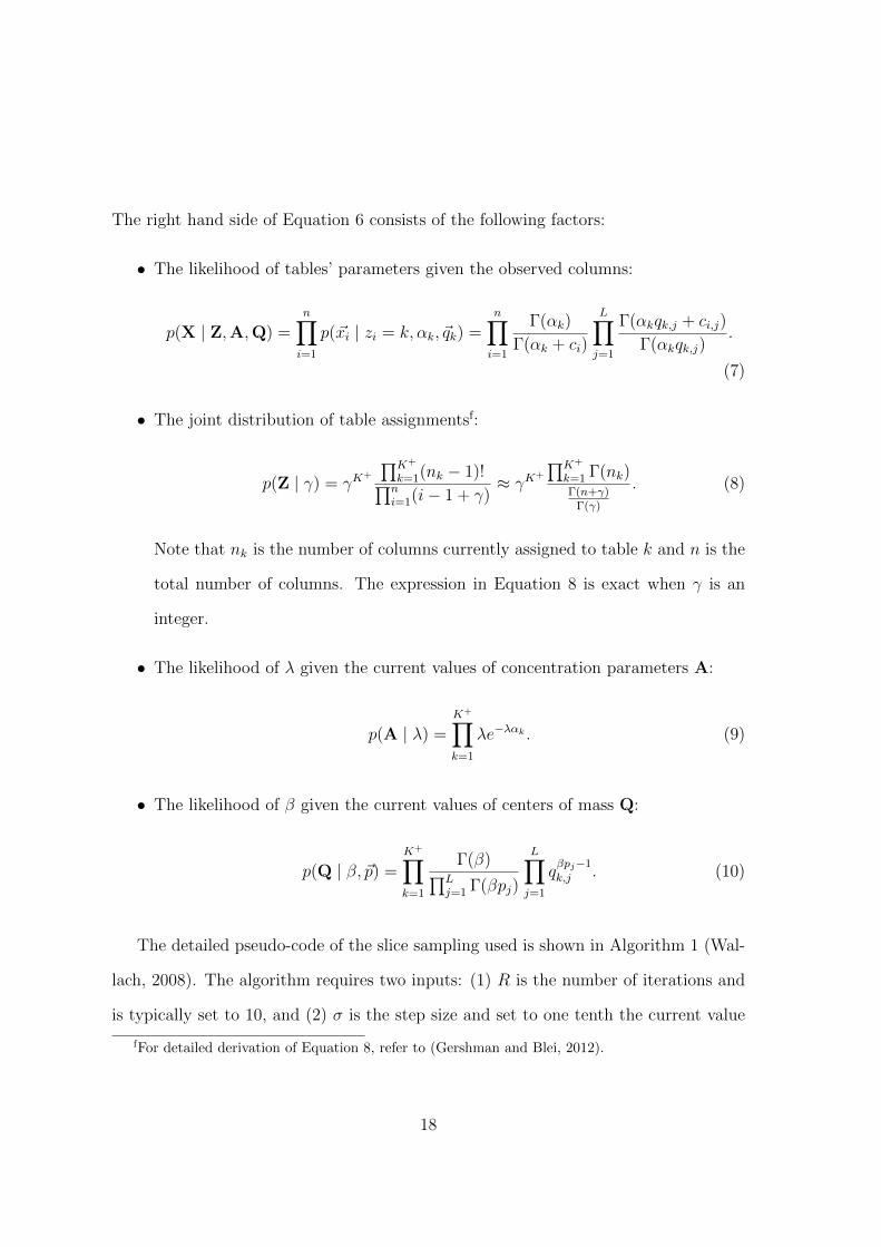
The right hand side of Equation 6 consists of the following factors:
• The likelihood of tables’ parameters given the observed columns:
p(X | Z,A,Q) =n∏
i=1
p(~xi | zi = k, αk, ~qk) =n∏
i=1
Γ(αk)
Γ(αk + ci)
L∏
j=1
Γ(αkqk,j + ci,j)
Γ(αkqk,j).
(7)
• The joint distribution of table assignmentsf:
p(Z | γ) = γK+
∏K+
k=1(nk − 1)!∏ni=1(i− 1 + γ)
≈ γK+
∏K+
k=1 Γ(nk)Γ(n+γ)
Γ(γ)
. (8)
Note that nk is the number of columns currently assigned to table k and n is the
total number of columns. The expression in Equation 8 is exact when γ is an
integer.
• The likelihood of λ given the current values of concentration parameters A:
p(A | λ) =K+∏
k=1
λe−λαk . (9)
• The likelihood of β given the current values of centers of mass Q:
p(Q | β, ~p) =K+∏
k=1
Γ(β)∏Lj=1 Γ(βpj)
L∏
j=1
qβpj−1k,j . (10)
The detailed pseudo-code of the slice sampling used is shown in Algorithm 1 (Wal-
lach, 2008). The algorithm requires two inputs: (1) R is the number of iterations and
is typically set to 10, and (2) σ is the step size and set to one tenth the current value
fFor detailed derivation of Equation 8, refer to (Gershman and Blei, 2012).
18
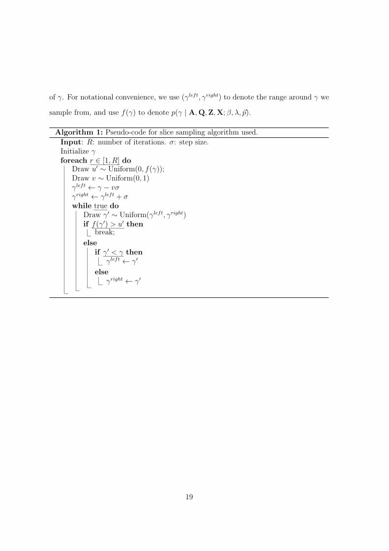
of γ. For notational convenience, we use (γleft, γright) to denote the range around γ we
sample from, and use f(γ) to denote p(γ | A,Q,Z,X; β, λ, ~p).
Algorithm 1: Pseudo-code for slice sampling algorithm used.
Input: R: number of iterations. σ: step size.Initialize γforeach r ∈ [1, R] do
Draw u′ ∼ Uniform(0, f(γ));Draw v ∼ Uniform(0, 1)γleft ← γ − vσγright ← γleft + σwhile true do
Draw γ′ ∼ Uniform(γleft, γright)if f(γ′) > u′ then
break;
elseif γ′ < γ then
γleft ← γ′
elseγright ← γ′
19
3 Results
The research group at UCSC that first proposed Dirichlet mixtures for protein analy-
sis currently makes a number of multiple alignment datasets available on their web
site, http://compbio.soe.ucsc.edu/dirichlets/index.html. We consider their dataset
“diverse-1216-uw”, called SUCSC here, which was studied also in (Ye et al., 2011b).
SUCSC consists of 23,903,805 amino acids arranged into 314,585 columns, and thus
containing a mean of approximately 76.0 amino acids per column.
3.1 The quality of Dirichlet mixtures
It is useful to have an objective measure for the quality of a DM, and for this purpose
we turn to the Minimum Description Length (MDL) principle (Grunwald, 2007), whose
essentials we review here.
One may define the description length of a dataset S, given a theory θ, as DL(S|θ) ≡
− log2 Pθ(S), i.e. the negative log of the probability for the dataset implied by the
theory. Because the logarithm is to the base 2, DL is said to be expressed in bits. This
definition may be extended to a model M by defining DL(S|M) ≡ infθ∈M DL(S|θ).
If one wishes to find the model that best describes a set of data, using DL alone
as a criterion is problematic because, for nested models, increasing the number of
parameters can only decrease DL. Accordingly, MDL theory introduces the formal
concept of the complexity of a model COMP(M) (Grunwald, 2007), which may be
thought of, intuitively, as the log of the effective number of independent theories the
model contains. The MDL principle then asserts that the model best justified by a
set of data is that which minimizes COMP(M) + DL(S|M). In essence, the principle
supports a theory drawn from a model of greater complexity only when this increased
20
complexity is offset by a sufficient decrease in data description length.
To select among Dirichlet mixture models DM with a variable number M of com-
ponents using the MDL principle, one must be able at least to approximate both
COMP(DM) and DL(S|DM). Heuristic arguments (Ye et al., 2011b) have extended
to COMP(DM) an analytic formula for the complexity of a single-component Dirichlet
model (Yu and Altschul, 2011). Calculating DL(S|DM) entails finding the maximum-
likelihood M -component DM. This is an instance of the classic hard problem of op-
timization within a rough but correlated high-dimensional space, and approximation
algorithms have been based on expectation maximization (EM) (Brown et al., 1993)
and Gibbs sampling (Ye et al., 2011b).
For the sake of analysis, we may treat our DP-sampler as simply an improved algo-
rithm for finding DMs that minimize total description length. To evaluate a particular
DM, we compare it to the baseline multinomial model in which all amino acids are
drawn randomly according to background probabilities ~p inferred from the data. For
this model, the description length of SUCSC is 99,604,971 bits, and the complexity of the
model is 206 bits (Ye et al., 2011b), so the total description length can be expressed
as 4.1669 bits/amino acid. We assess a DM by the decrease ∆ (bits/a.a.) in total
description length it implies with respect to this baseline, and use ∆ as an objective
function of mixture quality.
3.2 The optimal number of Dirichlet components
Our DP-sampling procedure does not converge on a unique DM, and selecting different
parameters β and γ of course yields different results. However, given a set of real
protein multiple alignment data, the results produced by the procedure after several
hundred iterations share various broad qualitative and quantitative features, which we
21
describe here.
At a given iteration, the current DM generated by the DP-sampler typically con-
tains many components to which only a small number of columns are assigned. These
components are particularly unstable, and with further iterations tend either to evapo-
rate or to grow in the number of associated columns. In general, they are unsupported
by the MDL principle when seeking a DM that maximizes ∆. Thus, after any given
iteration, we first arrange the sampler-generated Dirichlet components in decreasing
order of their number of associated columns, and then calculate the ∆ implied by
the DMs consisting of increasing numbers of these components. Although this greedy
method does not necessarily identify the optimal subset, it provides a reasonable ap-
proximation. Typically, the MDL principle excludes sets of components to which, in
aggregate, less than 2% of the columns are associated, with no single excluded compo-
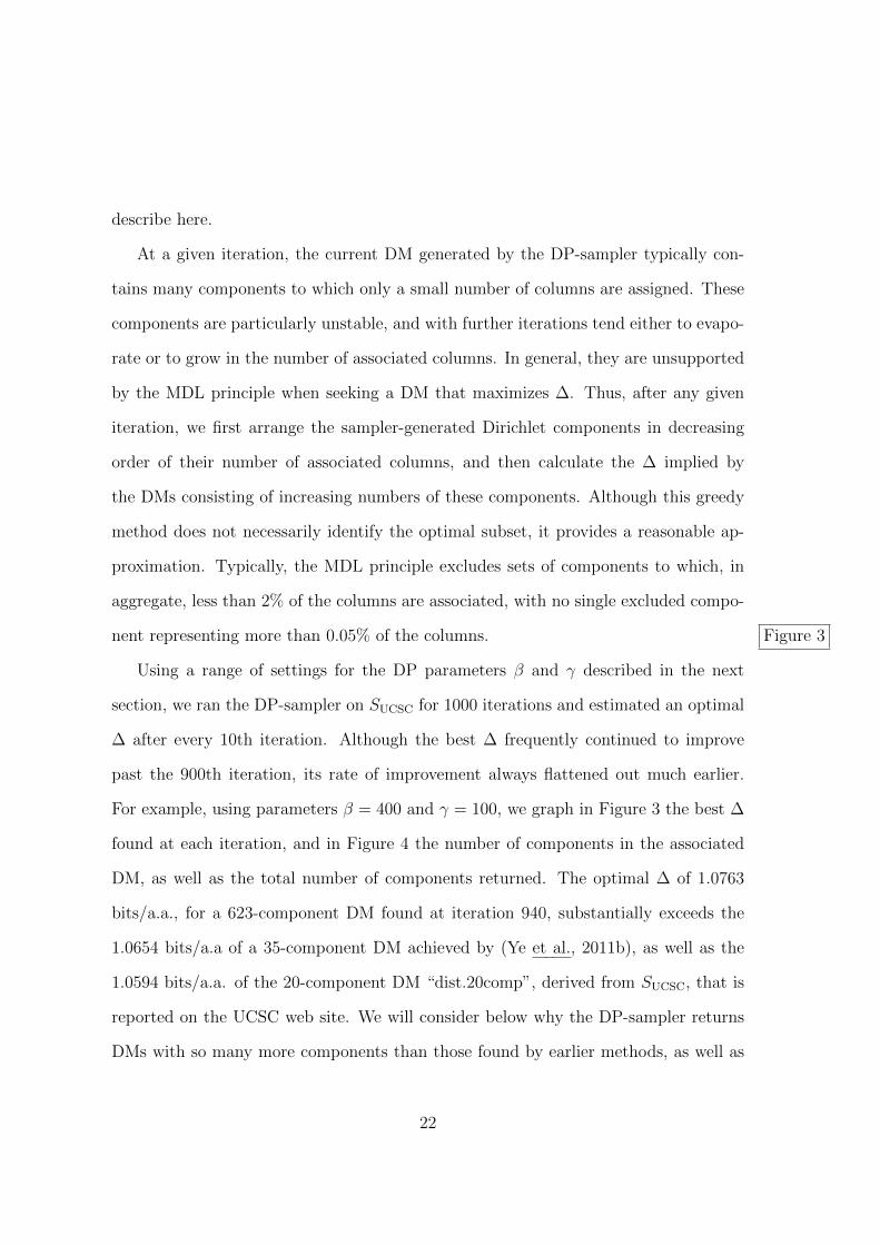
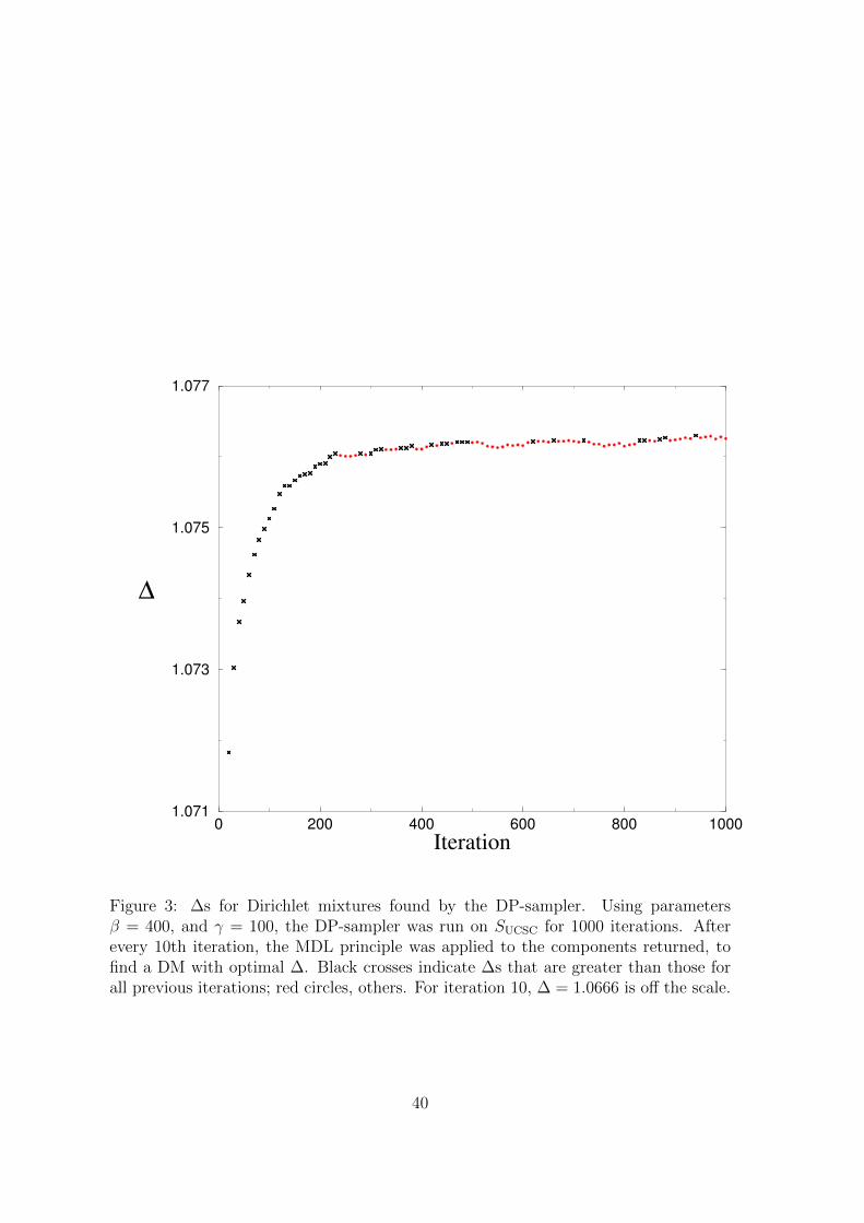
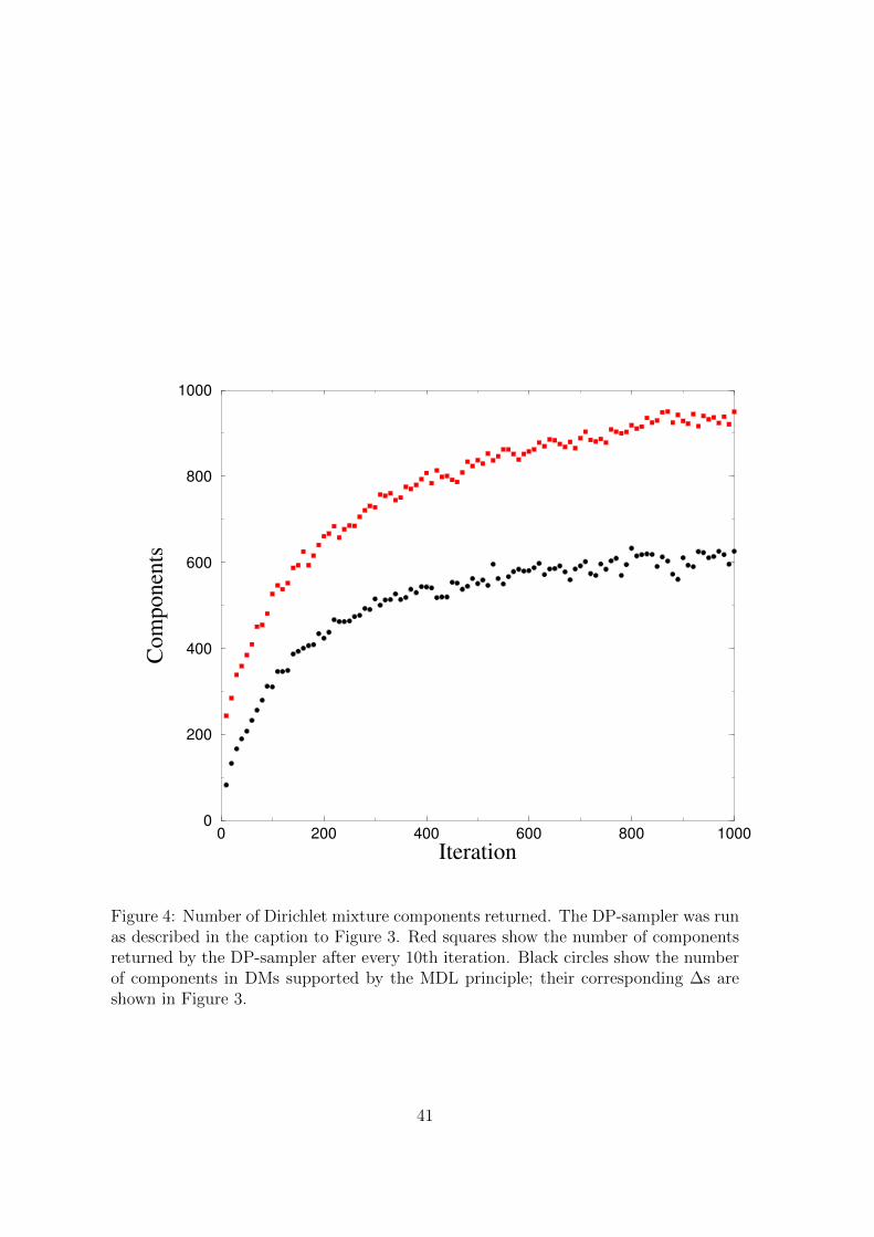
nent representing more than 0.05% of the columns. Figure 3
Using a range of settings for the DP parameters β and γ described in the next
section, we ran the DP-sampler on SUCSC for 1000 iterations and estimated an optimal
∆ after every 10th iteration. Although the best ∆ frequently continued to improve
past the 900th iteration, its rate of improvement always flattened out much earlier.
For example, using parameters β = 400 and γ = 100, we graph in Figure 3 the best ∆
found at each iteration, and in Figure 4 the number of components in the associated
DM, as well as the total number of components returned. The optimal ∆ of 1.0763
bits/a.a., for a 623-component DM found at iteration 940, substantially exceeds the
1.0654 bits/a.a of a 35-component DM achieved by (Ye et al., 2011b), as well as the
1.0594 bits/a.a. of the 20-component DM “dist.20comp”, derived from SUCSC, that is
reported on the UCSC web site. We will consider below why the DP-sampler returns
DMs with so many more components than those found by earlier methods, as well as
22
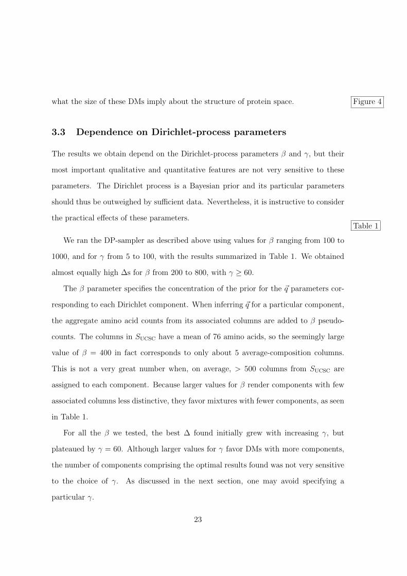
what the size of these DMs imply about the structure of protein space. Figure 4
3.3 Dependence on Dirichlet-process parameters
The results we obtain depend on the Dirichlet-process parameters β and γ, but their
most important qualitative and quantitative features are not very sensitive to these
parameters. The Dirichlet process is a Bayesian prior and its particular parameters
should thus be outweighed by sufficient data. Nevertheless, it is instructive to consider
the practical effects of these parameters.Table 1
We ran the DP-sampler as described above using values for β ranging from 100 to
1000, and for γ from 5 to 100, with the results summarized in Table 1. We obtained
almost equally high ∆s for β from 200 to 800, with γ ≥ 60.
The β parameter specifies the concentration of the prior for the ~q parameters cor-
responding to each Dirichlet component. When inferring ~q for a particular component,
the aggregate amino acid counts from its associated columns are added to β pseudo-
counts. The columns in SUCSC have a mean of 76 amino acids, so the seemingly large
value of β = 400 in fact corresponds to only about 5 average-composition columns.
This is not a very great number when, on average, > 500 columns from SUCSC are
assigned to each component. Because larger values for β render components with few
associated columns less distinctive, they favor mixtures with fewer components, as seen
in Table 1.
For all the β we tested, the best ∆ found initially grew with increasing γ, but
plateaued by γ = 60. Although larger values for γ favor DMs with more components,
the number of components comprising the optimal results found was not very sensitive
to the choice of γ. As discussed in the next section, one may avoid specifying a
particular γ.
23
One may prefer DMs with fewer components for algorithmic reasons. In this case,
it may be advantageous to use both large β and small γ; this tends to favor DMs with
fewer components, and thus to improve their corresponding ∆s. We consider below
the tradeoff of Dirichlet mixture size and accuracy.
3.4 Slice sampling γ
To avoid the arbitrariness of specifying a particular value for a DP parameter, or
the time involved in testing multiple values, we may use the slice sampling procedure
described above. In brief, after a given iteration of the DP-sampling algorithm, we
sample a new value γ′ within a range centered on the current value γ. We then compute
the likelihood of the current mixture model with this new γ′. If this likelihood is greater
than the likelihood with the current γ, there is a high probability that we will accept
this new γ′ and use it in the next iteration.
We implemented this sampling procedure for the DP parameter γ, using an initial
value of γ = 50, and a “burn-in” period of 25 iterations before γ is allowed to vary.
For β ranging from 200 to 1000, we ran this refined algorithm for 1000 iterations; for
β = 100 the program terminated after 323 iterations because the number of components
it generated exceeded a limit imposed by memory constraints. In Table 2, we report for
each β the mean and standard deviation for γ during the program’s last 100 iterations.
We also report the optimal ∆ found, its corresponding number of components, the
iteration yielding this ∆, and the value of γ during this iteration.Table 2
As can be seen, slice sampling converges on a relatively small range of values for
γ, and the best ∆ found is always within 0.0001 bits/a.a. of the best yielded by the
multiple searches shown in Table 1, which employ fixed, specified γ. As before, β ≈ 400
appears optimal, but this conclusion is now reached by a one-parameter rather than a
24
two-parameter search.
One may employ slice sampling to determine β as well as γ, but doing so is problem-
atic. Although we have being using ∆ as an objective function for Dirichlet mixtures,
the DP-sampler is ignorant of this function, instead sampling mixtures according their
posterior likelihood, given the prior imposed by the Dirichlet process. Indeed, the DP-
sampler returns mixtures with many more components than supported by the MDL
principle, as seen in Figure 4. We have been able to elide this inconsistency because, for
fixed β, greater posterior likelihoods for the larger mixtures correlate well with greater
values for ∆. This correlation is broken, however, once β may vary. The generalized
DP-sampler then prefers small β, yielding mixtures with many components, which are
penalized by the model-complexity term of the MDL principle.
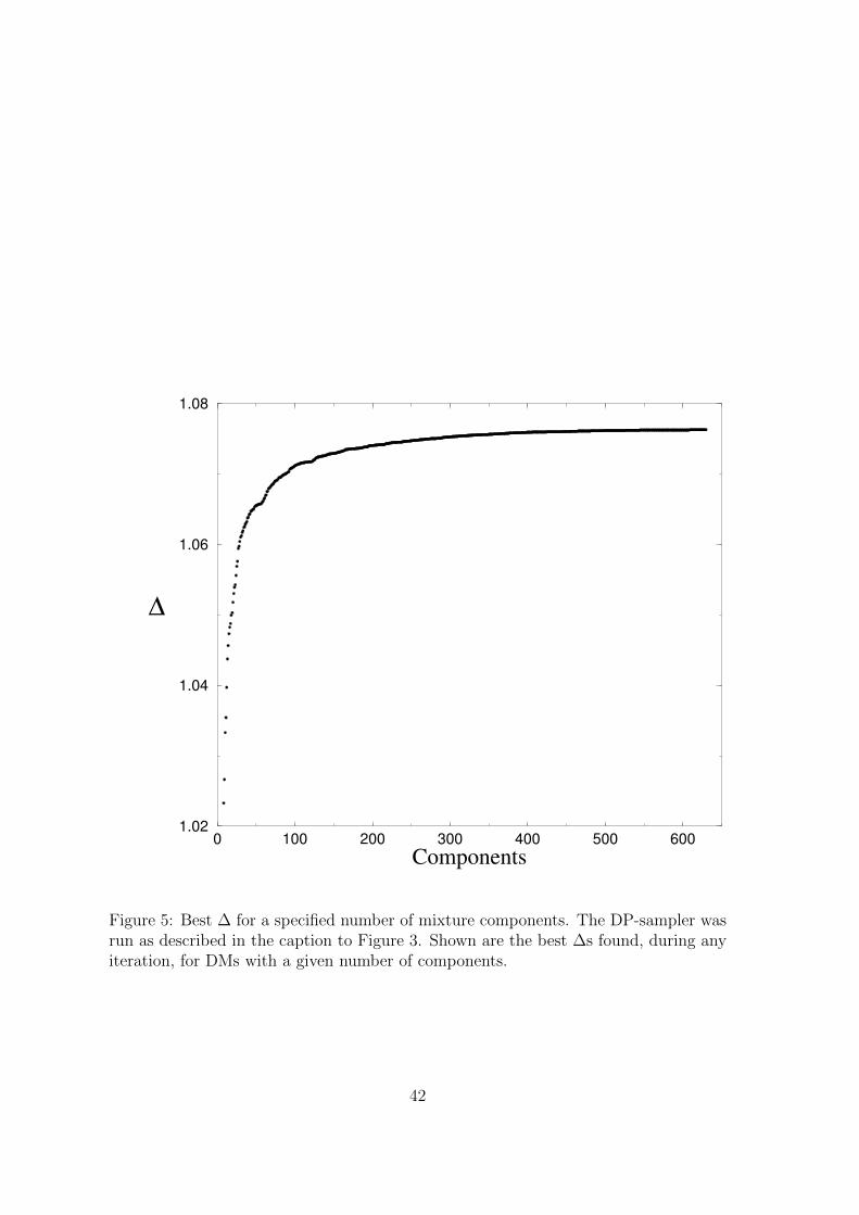
3.5 Tradeoff of ∆ and the number of Dirichlet components
So far we have been concerned only with maximizing ∆. However, DMs are derived for
use in profile-sequence, profile-profile, or multiple alignment programs (Brown et al.,
1993; Edgar and Sjolander, 2004; Altschul et al., 2010; Ye et al., 2011a), and in these
applications DMs with fewer components have a speed advantage. As seen in Fig-
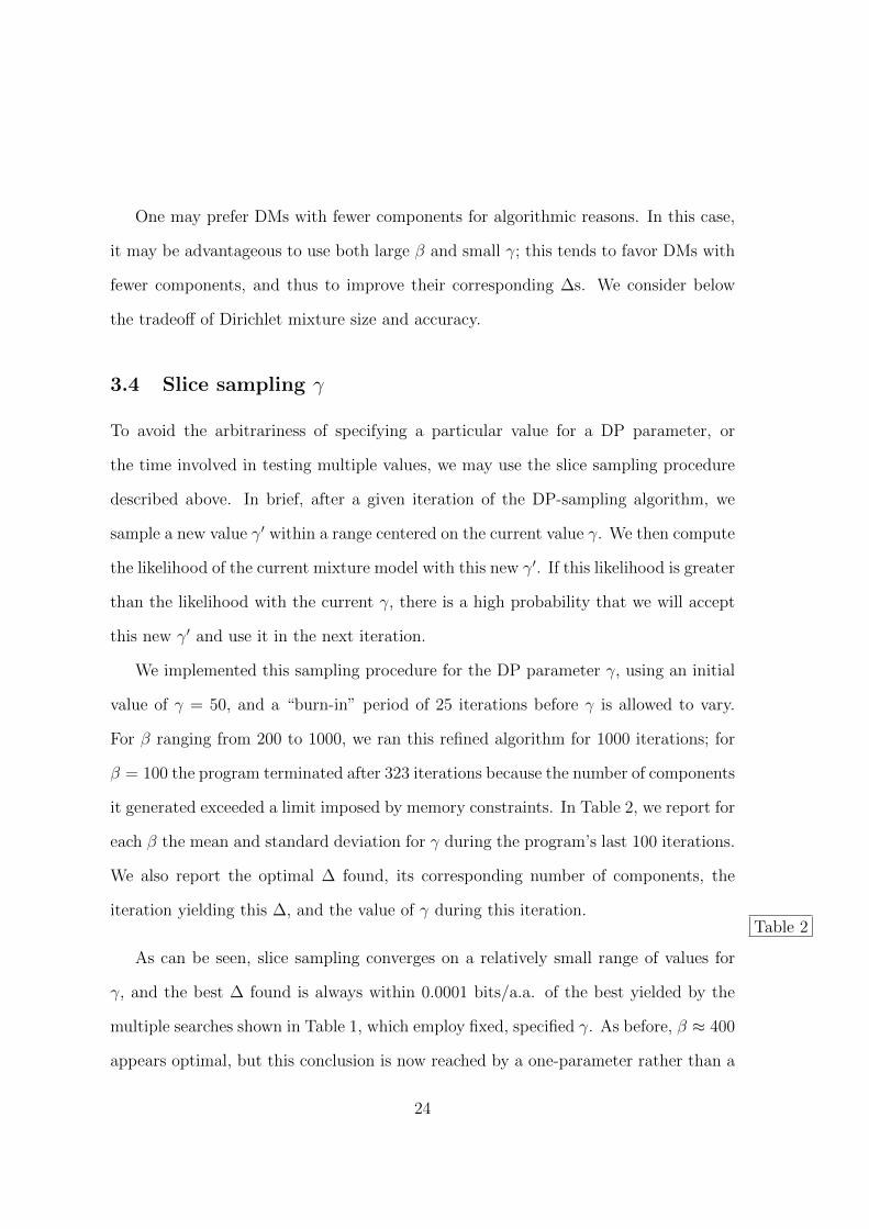
ure 3 and Figure 4, DMs with only slightly sub-optimal ∆ can have significantly fewer
components, and such DMs may well be preferred in certain circumstances.
To study this tradeoff explicitly, we recorded over all iterations of the run described
in Figures 3 and 4, as well as the greedy DM-construction procedure described above,
the greatest ∆ found for DMs with varying numbers of components; the results are
shown in Figure 5. A particular application, implementation, and preference for speed
vrs. DM accuracy (i.e. ∆) can be used with such a curve to derive an optimal DM size
from a software engineering perspective. Figure 5
25
3.6 The topography of protein space
What do the hundreds of Dirichlet components returned by the DP-sampler imply
about proteins? To study this question, it is useful to develop a representation of
DMs that is easier to comprehend than would be a mere tabulation of thousands of
parameters. The approach we take is to represent each component of a DM by a single
line of text. On this line, we focus primarily on the component’s center-of-mass vector
~q, which we represent by a string ~σ of twenty symbols, although we also report the
component’s mixture parameter w and concentration parameter α numerically.
In constructing the ~σ to represent a Dirichlet component, it is useful first to order the
amino acids in a manner that corresponds to their mutual similarities, even though any
linear arrangement must elide some of these multi-dimensional relationships. Various
orders have previously been proposed (Swanson, 1984; Brown et al., 1993), but our
data suggest the order “RKQEDNHWYFMLIVCTSAGP”, using the one-letter amino
acid code.
Because within proteins the amino acids occur with widely differing background
frequencies pj, it is fruitful to represent a Dirichlet component’s mean “target frequen-
cies” qj in relation to the corresponding pj. Accordingly, we base the symbol σj on the
implied “log-odds score” sj = log2(qj/pj) according to the following system:
26
sj > 2 σj = The amino acid’s one-letter code, in upper case
2 ≥ sj > 1 σj = The amino acid’s one-letter code, in lower case
1 ≥ sj > 0.5 σj = “+”
0.5 ≥ sj > −1 σj = “ ”
−1 ≥ sj > −2 σj = “.”
−2 ≥ sj > −4 σj = “-”
−4 ≥ sj σj = “=”
In other words, for a particular component, an upper case letter implies that the
frequency of the corresponding amino acid is enriched vis-a-vis background by a factor
greater than 4.0, while the symbol “=” means it is decreased by a factor of at least 16.
We choose such a positive/negative asymmetry among the categories for defining the
σj because qj ∈ (0, 1) implies an upper bound on sj, but no lower bound.
As seen in Table 1, the DMs with greatest ∆ can have over 600 components. Al-
though we could analyze mixtures of this size, most of their important qualitative
features are apparent in mixtures with many fewer components, so we will consider
such a smaller DM here. As discussed above, ∆ for DMs with fewer components tends
to be optimized using relatively large β and small γ. Choosing β = 1000 and γ = 10,
and requiring an improvement of at least 4 × 10−5 bits/a.a. in ∆ for each additional
component, our best result was a 134-component DM with ∆ = 1.0732 bits/a.a, which
we call θ134. The parameters associated with all components of θ134 are presented in
Tables 3–5.Table 3
A DM’s components may be listed in arbitrary order. One reasonable choice is by
decreasing order of mixture parameter w, and in Tables 3–5 we give the rank for each
component that such an ordering would yield. However, we have found it instructive to
divide θ134’s components into three groups, and to manually reorder the components of
27
each group, in order to elucidate several prominent features of the probability landscape
the DM represents. It may be possible to automate such a grouping and ordering using
distance measures between Dirichlet distributions (Rauber et al., 2008). Developing
such a method would be of interest, but for our present purposes it would provide only
a distraction.Table 4
Perhaps the most important feature of θ134 is represented by the 98 components of
Group A (Table 3). As one moves from one component to the next within this group,
the center of mass usually changes only slightly, and in a relatively continuous manner.
The superposition of the probability hills represented by individual components can
thus be visualized as a probability ridge threading its way through Ω20, with several
minor spurs.
The second feature of θ134 is represented by the 17 components of Group B (Table 4),
which share two main properties: a preference for the amino acids glycine (G) and/or
proline (P), and an aversion to hydrophobic amino acids. This group of components
can be seen as a secondary ridge, separated from the first.Table 5
A third feature is represented by the 19 components of Group C (Table 5). These
components strongly favor a single amino acid, without clear secondary preferences that
would attach them to the major ridge of Group A. Of note is the last component in this
group, whose concentration parameter α is very close to 0. This implies a probability
density concentrated almost completely near the vertices of Ω20. It is a peculiarity
of DMs that such densities can be approximated either by a single component with
small α and probability mass dominated by several letters, or by the superposition of
multiple components each with large α and probability mass dominated by a single
letter. Thus this last component can be seen, in essence, as a formal alternative to the
type of probability density represented by the other components of Group C.
28
In general, it may seem surprising that the data will support the identification of the
134 Dirichlet components shown in Tables 3–5, not to mention the > 600 components
of many DMs with greater ∆. However, the > 300,000 columns in SUCSC can associate
on average > 500 columns to each of 600 components, and this much data is able to
support relatively fine distinctions between similar probability densities.
When one compares different mixtures returned by the DP-sampler, the overall
shape of the probability densities they describe can be recognized as remarkably similar.
In contrast, the parameters of the individual components that go into approximating
this shape have no particular stability. For example, a point that is halfway between the
crests of two components in one mixture may very well be at the crest of an individual
component in another.
29
4 Conclusion
When a set of data is believed to be well described by a mixture distribution, but with
an unknown number of components, the Dirichlet process may be applied to infer the
mixture (Blei and Jordan, 2005). Because homologous positions within protein families
have been fruitfully described by Dirichlet mixtures (Brown et al., 1993; Sjolander et al.,
1996; Altschul et al., 2010), we have sought here to infer such mixtures from multiple
alignment data using a Gibbs sampling algorithm based upon the Dirichlet process.
This required us to develop several technical innovations, because the Dirichlet process
has not previously been applied to DMs.
In contrast to previous approaches (Brown et al., 1993; Sjolander et al., 1996; Ye
et al., 2011b), our DP-sampler yields many hundreds of Dirichlet components when
applied to real multiple alignment data. To understand these results, one should recog-
nize that DMs are employed to model proteins primarily for mathematical as opposed
to biological reasons: with Bayesian analysis, the posterior of a DM prior is still a
DM (Brown et al., 1993; Sjolander et al., 1996; Altschul et al., 2010). The DM for-
malism suggests the metaphor of discrete probability hills in Ω20, each representing a
category for classifying protein positions. However, the actual probability topography
in Ω20 that describes proteins appears to be qualitatively different, having, for exam-
ple, long probability ridges. To model such features well using Dirichlet components
requires a large number of them, with closely spaced centers of mass. Our analysis
suggests there is no “correct” number of components or categories for describing the
probability distribution over Ω20 implied by proteins. Instead, when the MDL principle
is applied, steadily increasing amounts of data should support steadily increasing num-
bers of components. However, as the number of components grows, there is also steadily
30
diminishing improvement, as measured by ∆, in modeling the underlying probability
distribution.
The DP-sampler is able to find DMs that model multiple alignment data better
than do those mixtures found by previously proposed methods. A key to its relative
success is its ability to seed new components with columns that are not modeled well
by any existing components, but to abandon components that do not then attract
other columns. This fosters a much more efficient search of the very high-dimensional
Dirichlet-mixture space than does seeding the space with random starting positions.
Although existing multiple alignment data sets may support DMs with over 500
components, speed considerations may favor smaller mixtures for use in practical se-
quence comparison algorithms. The DP-sampler can generate mixtures of many differ-
ent sizes, to facilitate such a tradeoff.
At a deeper level, the DP-sampler provides a new perspective on the topography of
protein space. This perspective suggests that the amino acid preferences at individual
protein positions should, in general, be thought of not as falling into one of several
categories, but rather as arrayed along a continuum. These preferences, represented
by points in Ω20, fall mainly near a long, almost one-dimensional probability ridge
winding through the space. This perspective may suggest interesting questions for
further investigation. For example, multiple alignment columns that imply similar
high likelihoods for components situated far from one another along the ridge might
imply either misalignment, or the presence of distinct protein subfamilies within the
alignment.
31

Acknowledgments
Jordan Boyd-Graber is supported by NSF grant #1018625. Stephen Altschul is sup-
ported by the Intramural Research Program of the National Library of Medicine at the
National Institutes of Health.
32
References
Aldous, D. 1985. Exchangeability and related topics. In Ecole d’Ete de Probabilities
de Saint-Flour XIII 1983, 1–198. Springer.
Altschul, S. F., Wootton, J. C., Zaslavsky, E. et al. 2010. The construction and use of
log-odds substitution scores for multiple sequence alignment. PLoS Comp. Biol. 6,
e1000852.
Antoniak, C. E. 1974. Mixtures of Dirichlet processes with applications to Bayesian
nonparametric problems. Ann. Stat. 2, 1152–1174.
Beal, M. J., Ghahramani, Z., and Rasmussen, C. E. 2002. The infinite hidden Markov
model. In Adv. Neural Inf. Process. Syst. MIT Press.
Blei, D. M. and Jordan, M. I. 2005. Variational inference for Dirichlet process mixtures.
J. Bayesian Anal. 1, 121–144.
Blei, D. M., Ng, A., and Jordan, M. 2003. Latent Dirichlet allocation. J. Mach. Learn.
Res. 3, 993–1022.
Brown, M., Hughey, R., Krogh, A. et al. 1993. Using Dirichlet mixture priors to derive
hidden Markov models for protein families. In Proc. First International Conf. on
Intell. Syst. for Mol. Biol., 47–55. AAAI Press.
Edgar, R. C. and Sjolander, K. 2004. A comparison of scoring functions for protein
sequence profile alignment. Bioinformatics 20, 1301–1308.
Engen, S. 1975. A note on the geometric series as a species frequency model. Biometrika
62, pp. 697–699.
33
Ferguson, T. S. 1973. A Bayesian analysis of some nonparametric problems. Ann. Stat.
1, 209–230.
Gershman, S. J. and Blei, D. M. 2012. A tutorial on Bayesian nonparametric models.
J. Math. Psych. 56, 1–12.
Griffiths, R. 1980. Lines of descent in the diffusion approximation of neutral Wright-
Fisher models. Theoretical Population Biol. 17, 37–50.
Grunwald, P. D. 2007. The Minimum Description Length Principle, MIT Press Books,
volume 1. The MIT Press.
Hannah, L., Blei, D. M., and Powell, W. B. 2011. Dirichlet process mixtures of gener-
alized linear models. J. Mach. Learn. Res. 12, 1923–1953.
Hardisty, E., Boyd-Graber, J., and Resnik, P. 2010. Modeling perspective using adaptor
grammars. In In Proc. Conf. Empirical Methods in Natural Language Processing.
Lewis, D. D. 1998. Naive (Bayes) at forty: The independence assumption in information
retrieval. In European Conf. on Mach. Learn., ECML ’98, 4–15.
McCloskey, J. 1965. A Model for the Distribution of Individuals by Species in an
Environment. Ph.D. thesis, Department of Statistics, Michigan State University.
(Unpublished).
Minka, T. P. 2000. Estimating a Dirichlet distribution. Technical report, Microsoft.
Muller, P. and Quintana, F. A. 2004. Nonparametric Bayesian data analysis. Statist.
Sci. 19, 95–110.
Neal, R. M. 2003. Slice sampling. Ann. Stat. 31, 705–767.
34
Pitman, J. and Yor, M. 1997. The two-parameter Poisson-Dirichlet distribution derived
from a stable subordinator. Ann. Probab. 25, 855–900.
Rauber, T. W., Braun, T., and Berns, K. 2008. Probabilistic distance measures of the
Dirichlet and Beta distributions. Pattern Recogn. 41, 637–645.
Sethuraman, J. 1994. A constructive definition of Dirichlet priors. Statistica Sinica 4,
639–650.
Sjolander, K., Karplus, K., Brown, M. et al. 1996. Dirichlet mixtures: a method for
improved detection of weak but significant protein sequence homology. Comput.
Appl. Biosci. 12, 327–345.
Swanson, R. 1984. A vector representation for amino acid sequences. Bull. Math. Biol.
46, 623–639.
Teh, Y. W., Jordan, M. I., Beal, M. J. et al. 2006. Hierarchical Dirichlet processes. J.
Amer. Statist. Assoc. 101, 1566–1581.
Wallach, H. M. 2008. Structured Topic Models for Language. Ph.D. thesis, University
of Cambridge.
Ye, X., Wang, G., and Altschul, S. F. 2011a. An assessment of substitution scores for
protein profile-profile comparison. Bioinformatics 27, 3356–3363.
Ye, X., Yu, Y.-K., and Altschul, S. F. 2011b. On the inference of Dirichlet mixture
priors for protein sequence comparison. J. Comput. Biol. 18, 941–954.
Yu, Y.-K. and Altschul, S. F. 2011. The complexity of the Dirichlet model for multiple
alignment data. J. Comput. Biol. 18, 925–939.
35
List of Figures
1 Density plots for four Dirichlet distributions. The densities are over
the triangular simplex that represents multinomial distributions over
three letters, and demonstrate how different Dirichlet components can
accommodate variable concentrations. Darker coloring denotes higher
probability density. (a) Dirichlet parameters that are all 1.0 yield a
uniform density over multinomial distributions. (b) Dirichlet parameters
that are all greater than 1.0 yield a density concentrated near the mean
~q, in this case (0.6250, 0.0625, 0.3125). (c) and (d) Dirichlet parameters
that are all less than 1.0 yield a density concentrated near the edges
and corners of the simplex. Such a density favors sparse multinomials,
in which only a subset of letters has appreciable probability. Symmetric
(c) and asymmetric (d) cases are shown. . . . . . . . . . . . . . . . . . 37
2 Graphical model representing the Dirichlet process Dirichlet mixture
model proposed in this paper. Nodes represent variables; shaded nodes
are observed; edges show probabilistic dependencies; and plates denote
replication. . . . . . . . . . . . . . . . . . . . . . . . . . . . . . . . . . 38
3 ∆s for Dirichlet mixtures found by the DP-sampler. Using parameters
β = 400, and γ = 100, the DP-sampler was run on SUCSC for 1000
iterations. After every 10th iteration, the MDL principle was applied to
the components returned, to find a DM with optimal ∆. Black crosses
indicate ∆s that are greater than those for all previous iterations; red
circles, others. For iteration 10, ∆ = 1.0666 is off the scale. . . . . . . . 39
36
4 Number of Dirichlet mixture components returned. The DP-sampler
was run as described in the caption to Figure 3. Red squares show the
number of components returned by the DP-sampler after every 10th it-
eration. Black circles show the number of components in DMs supported
by the MDL principle; their corresponding ∆s are shown in Figure 3. . 40
5 Best ∆ for a specified number of mixture components. The DP-sampler
was run as described in the caption to Figure 3. Shown are the best ∆s
found, during any iteration, for DMs with a given number of components. 41
37
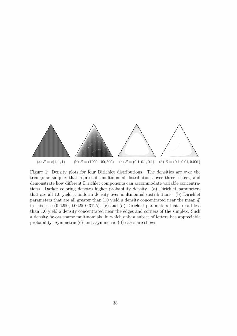
(a) ~α = e(1, 1, 1) (b) ~α = (1000, 100, 500) (c) ~α = (0.1, 0.1, 0.1) (d) ~α = (0.1, 0.01, 0.001)
Figure 1: Density plots for four Dirichlet distributions. The densities are over thetriangular simplex that represents multinomial distributions over three letters, anddemonstrate how different Dirichlet components can accommodate variable concentra-tions. Darker coloring denotes higher probability density. (a) Dirichlet parametersthat are all 1.0 yield a uniform density over multinomial distributions. (b) Dirichletparameters that are all greater than 1.0 yield a density concentrated near the mean ~q,in this case (0.6250, 0.0625, 0.3125). (c) and (d) Dirichlet parameters that are all lessthan 1.0 yield a density concentrated near the edges and corners of the simplex. Sucha density favors sparse multinomials, in which only a subset of letters has appreciableprobability. Symmetric (c) and asymmetric (d) cases are shown.
38
∞
Figure 2: Graphical model representing the Dirichlet process Dirichlet mixture modelproposed in this paper. Nodes represent variables; shaded nodes are observed; edgesshow probabilistic dependencies; and plates denote replication.
39
0 200 400 600 800 1000
Iteration
1.071
1.073
1.075
1.077
∆
Figure 3: ∆s for Dirichlet mixtures found by the DP-sampler. Using parametersβ = 400, and γ = 100, the DP-sampler was run on SUCSC for 1000 iterations. Afterevery 10th iteration, the MDL principle was applied to the components returned, tofind a DM with optimal ∆. Black crosses indicate ∆s that are greater than those forall previous iterations; red circles, others. For iteration 10, ∆ = 1.0666 is off the scale.
40
0 200 400 600 800 1000
Iteration
0
200
400
600
800
1000
Com
ponen
ts
Figure 4: Number of Dirichlet mixture components returned. The DP-sampler was runas described in the caption to Figure 3. Red squares show the number of componentsreturned by the DP-sampler after every 10th iteration. Black circles show the numberof components in DMs supported by the MDL principle; their corresponding ∆s areshown in Figure 3.
41
0 100 200 300 400 500 600
Components
1.02
1.04
1.06
1.08
∆
Figure 5: Best ∆ for a specified number of mixture components. The DP-sampler wasrun as described in the caption to Figure 3. Shown are the best ∆s found, during anyiteration, for DMs with a given number of components.
42
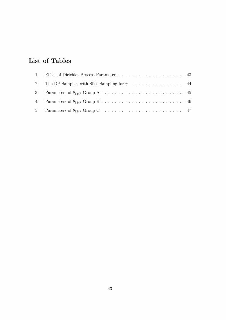
List of Tables
1 Effect of Dirichlet Process Parameters . . . . . . . . . . . . . . . . . . . 43
2 The DP-Sampler, with Slice Sampling for γ . . . . . . . . . . . . . . . 44
3 Parameters of θ134: Group A . . . . . . . . . . . . . . . . . . . . . . . . 45
4 Parameters of θ134: Group B . . . . . . . . . . . . . . . . . . . . . . . . 46
5 Parameters of θ134: Group C . . . . . . . . . . . . . . . . . . . . . . . . 47
43
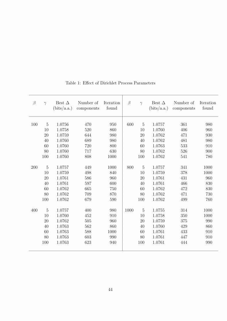
Table 1: Effect of Dirichlet Process Parameters
β γ Best ∆ Number of Iteration β γ Best ∆ Number of Iteration(bits/a.a.) components found (bits/a.a.) components found
100 5 1.0756 470 950 600 5 1.0757 361 98010 1.0758 520 860 10 1.0760 406 96020 1.0759 644 980 20 1.0762 471 93040 1.0760 689 980 40 1.0762 481 98060 1.0760 720 800 60 1.0763 533 91080 1.0760 717 630 80 1.0762 526 900
100 1.0760 808 1000 100 1.0762 541 780
200 5 1.0757 449 1000 800 5 1.0757 341 100010 1.0759 498 840 10 1.0759 378 100020 1.0761 586 960 20 1.0761 431 96040 1.0761 597 600 40 1.0761 466 83060 1.0762 665 750 60 1.0762 472 83080 1.0762 709 870 80 1.0762 471 730
100 1.0762 679 590 100 1.0762 499 760
400 5 1.0757 400 980 1000 5 1.0755 314 100010 1.0760 452 910 10 1.0758 350 100020 1.0762 505 960 20 1.0759 375 99040 1.0763 562 860 40 1.0760 429 86060 1.0763 588 1000 60 1.0761 433 91080 1.0763 603 990 80 1.0761 447 910
100 1.0763 623 940 100 1.0761 444 990
44

Table 2: The DP-Sampler, with Slice Sampling for γ
β Mean and standard Best ∆ Number of Iteration γdeviation of γ (bits/a.a.) components found
100 199.7± 13.0 1.0760 767 280 200200 183.9± 6.8 1.0762 721 580 166400 129.6± 4.3 1.0763 608 790 128600 95.5± 3.9 1.0762 537 930 94800 82.2± 3.5 1.0762 482 990 83
1000 66.8± 2.8 1.0760 442 940 69
45
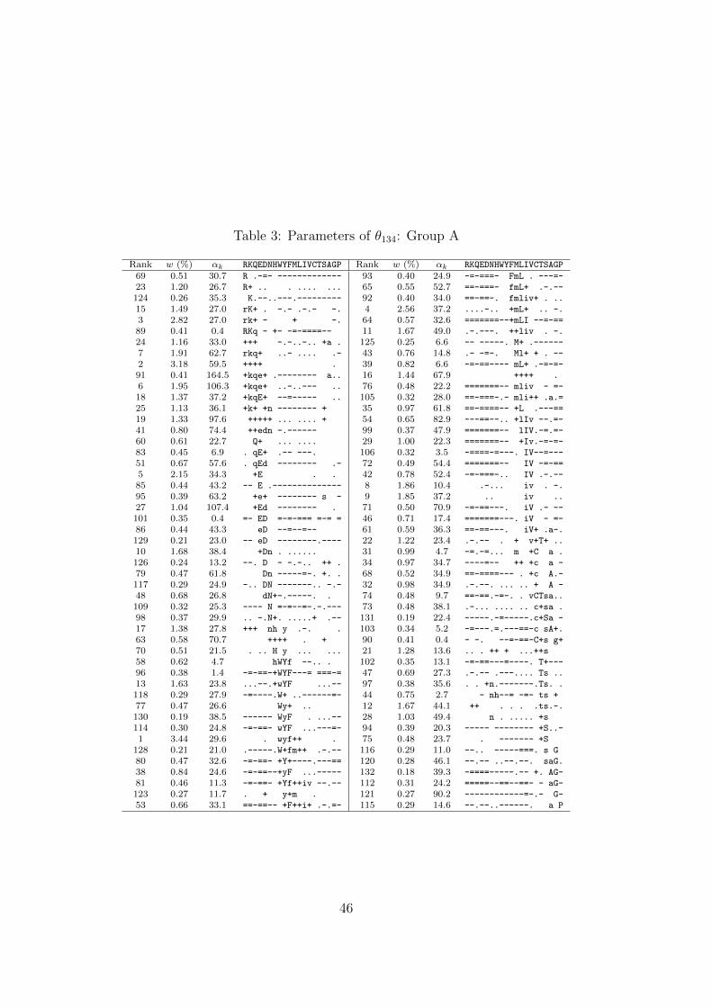
Table 3: Parameters of θ134: Group A
Rank w (%) αk RKQEDNHWYFMLIVCTSAGP Rank w (%) αk RKQEDNHWYFMLIVCTSAGP
69 0.51 30.7 R .-=- ------------- 93 0.40 24.9 -=-===- FmL . ---=-
23 1.20 26.7 R+ .. . .... ... 65 0.55 52.7 ==-===- fmL+ .-.--
124 0.26 35.3 K.--..---.--------- 92 0.40 34.0 ==-==-. fmliv+ . ..
15 1.49 27.0 rK+ . -.- .-.- -. 4 2.56 37.2 ....-.. +mL+ .. -.
3 2.82 27.0 rk+ - + -. 64 0.57 32.6 =======--+mLI --=-==
89 0.41 0.4 RKq - +- -=-====-- 11 1.67 49.0 .-.---. ++liv . -.
24 1.16 33.0 +++ -.-..-.. +a . 125 0.25 6.6 -- -----. M+ .------
7 1.91 62.7 rkq+ ..- .... .- 43 0.76 14.8 .- -=-. Ml+ + . --
2 3.18 59.5 ++++ . 39 0.82 6.6 -=-==---- mL+ .-=-=-
91 0.41 164.5 +kqe+ .-------- a.. 16 1.44 67.9 ++++ .
6 1.95 106.3 +kqe+ ..-..--- .. 76 0.48 22.2 =======-- mliv - =-
18 1.37 37.2 +kqE+ --=----- .. 105 0.32 28.0 ==-===-.- mli++ .a.=
25 1.13 36.1 +k+ +n -------- + 35 0.97 61.8 ==-====-- +L .---==
19 1.33 97.6 +++++ ... .... + 54 0.65 82.9 ---==--.. +lIv --.=-
41 0.80 74.4 ++edn -.------ 99 0.37 47.9 =======-- lIV.-=.=-
60 0.61 22.7 Q+ ... .... 29 1.00 22.3 =======-- +Iv.-=-=-
83 0.45 6.9 . qE+ .-- ---. 106 0.32 3.5 -====-=---. IV--=---
51 0.67 57.6 . qEd -------- .- 72 0.49 54.4 =======-- IV -=-==
5 2.15 34.3 +E . . 42 0.78 52.4 -=-===-.. IV .-.--
85 0.44 43.2 -- E .-------------- 8 1.86 10.4 .-... iv . -.
95 0.39 63.2 +e+ -------- s - 9 1.85 37.2 .. iv ..
27 1.04 107.4 +Ed -------- . 71 0.50 70.9 -=-==---. iV .- --
101 0.35 0.4 =- ED =-=-=== =-= = 46 0.71 17.4 =======---. iV - =-
86 0.44 43.3 eD --=--=-- 61 0.59 36.3 ==-==---. iV+ .a-.
129 0.21 23.0 -- eD --------.---- 22 1.22 23.4 .-.-- . + v+T+ ..
10 1.68 38.4 +Dn . ...... 31 0.99 4.7 -=.-=... m +C a .
126 0.24 13.2 --. D - -.-.. ++ . 34 0.97 34.7 ----=-- ++ +c a -
79 0.47 61.8 Dn -----=-. +. . 68 0.52 34.9 ==-====--- . +c A.-
117 0.29 24.9 -.. DN -------.. -.- 32 0.98 34.9 .-.--. ... .. + A -
48 0.68 26.8 dN+-.-----. . 74 0.48 9.7 ==-==.-=-. . vCTsa..
109 0.32 25.3 ---- N =-=--=-.-.--- 73 0.48 38.1 .-... .... .. c+sa .
98 0.37 29.9 .. -.N+. .....+ .-- 131 0.19 22.4 -----.-=-----.c+Sa -
17 1.38 27.8 +++ nh y .-. . 103 0.34 5.2 -=---.=.---==-c sA+.
63 0.58 70.7 ++++ . + 90 0.41 0.4 - -. --=-==-C+s g+
70 0.51 21.5 . .. H y ... ... 21 1.28 13.6 .. . ++ + ...++s
58 0.62 4.7 hWYf --.. . 102 0.35 13.1 -=-==---=----. T+---
96 0.38 1.4 -=-==-+WYF---= ===-= 47 0.69 27.3 .-.-- .---.... Ts ..
13 1.63 23.8 ...--.+wYF ...-- 97 0.38 35.6 . . +n.-------.Ts. .
118 0.29 27.9 -=----.W+ ..------=- 44 0.75 2.7 - nh--= -=- ts +
77 0.47 26.6 Wy+ .. 12 1.67 44.1 ++ . . . .ts.-.
130 0.19 38.5 ------ WyF . ...-- 28 1.03 49.4 n . ..... +s
114 0.30 24.8 -=-==- wYF ...---=- 94 0.39 20.3 ----- -------- +S..-
1 3.44 29.6 . wyf++ . 75 0.48 23.7 . ------- +S
128 0.21 21.0 .-----.W+fm++ .-.-- 116 0.29 11.0 --.. -----===. s G
80 0.47 32.6 -=-==- +Y+----.---== 120 0.28 46.1 --.-- ..--.--. saG.
38 0.84 24.6 -=-==--+yF ...----- 132 0.18 39.3 -====-----.-- +. AG-
81 0.46 11.3 -=-==- +Yf++iv --.-- 112 0.31 24.2 =====--==--==- - aG-
123 0.27 11.7 . + y+m . 121 0.27 90.2 ------------=-.- G-
53 0.66 33.1 ==-==-- +F++i+ .-.=- 115 0.29 14.6 --.--..------. a P
46
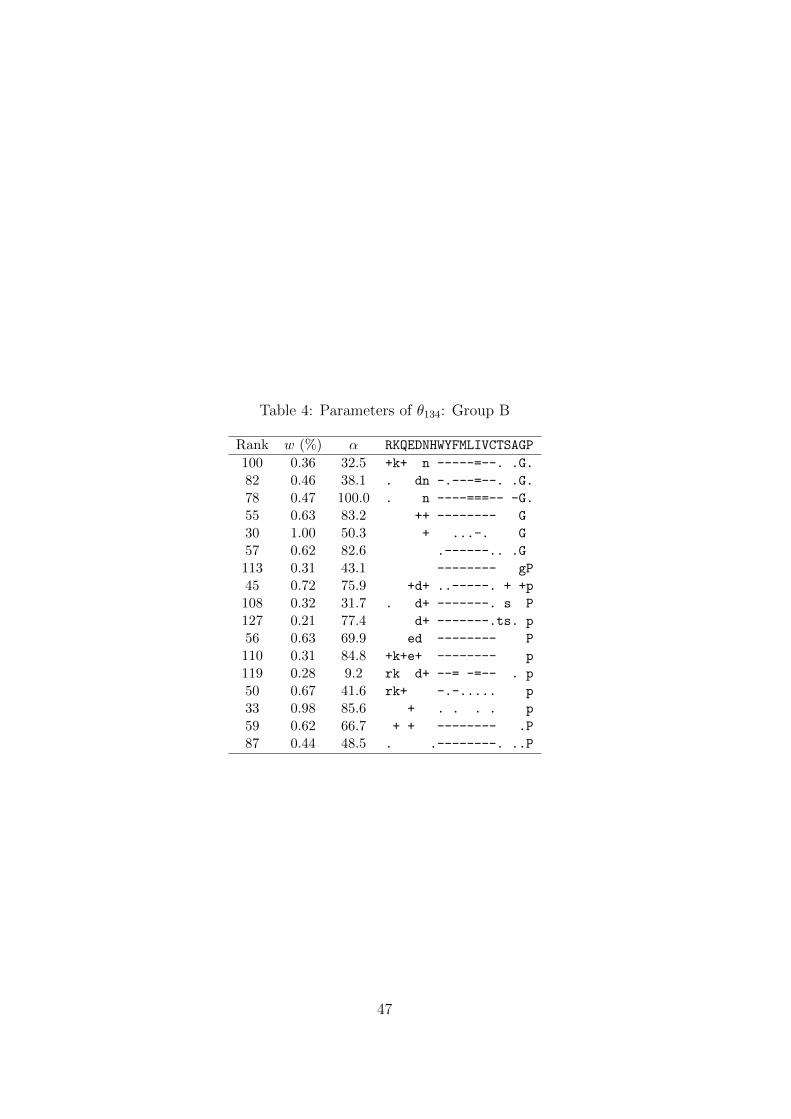
Table 4: Parameters of θ134: Group B
Rank w (%) α RKQEDNHWYFMLIVCTSAGP
100 0.36 32.5 +k+ n -----=--. .G.
82 0.46 38.1 . dn -.---=--. .G.
78 0.47 100.0 . n ----===-- -G.
55 0.63 83.2 ++ -------- G
30 1.00 50.3 + ...-. G
57 0.62 82.6 .------.. .G
113 0.31 43.1 -------- gP
45 0.72 75.9 +d+ ..-----. + +p
108 0.32 31.7 . d+ -------. s P
127 0.21 77.4 d+ -------.ts. p
56 0.63 69.9 ed -------- P
110 0.31 84.8 +k+e+ -------- p
119 0.28 9.2 rk d+ --= -=-- . p
50 0.67 41.6 rk+ -.-..... p
33 0.98 85.6 + . . . . p
59 0.62 66.7 + + -------- .P
87 0.44 48.5 . .--------. ..P
47
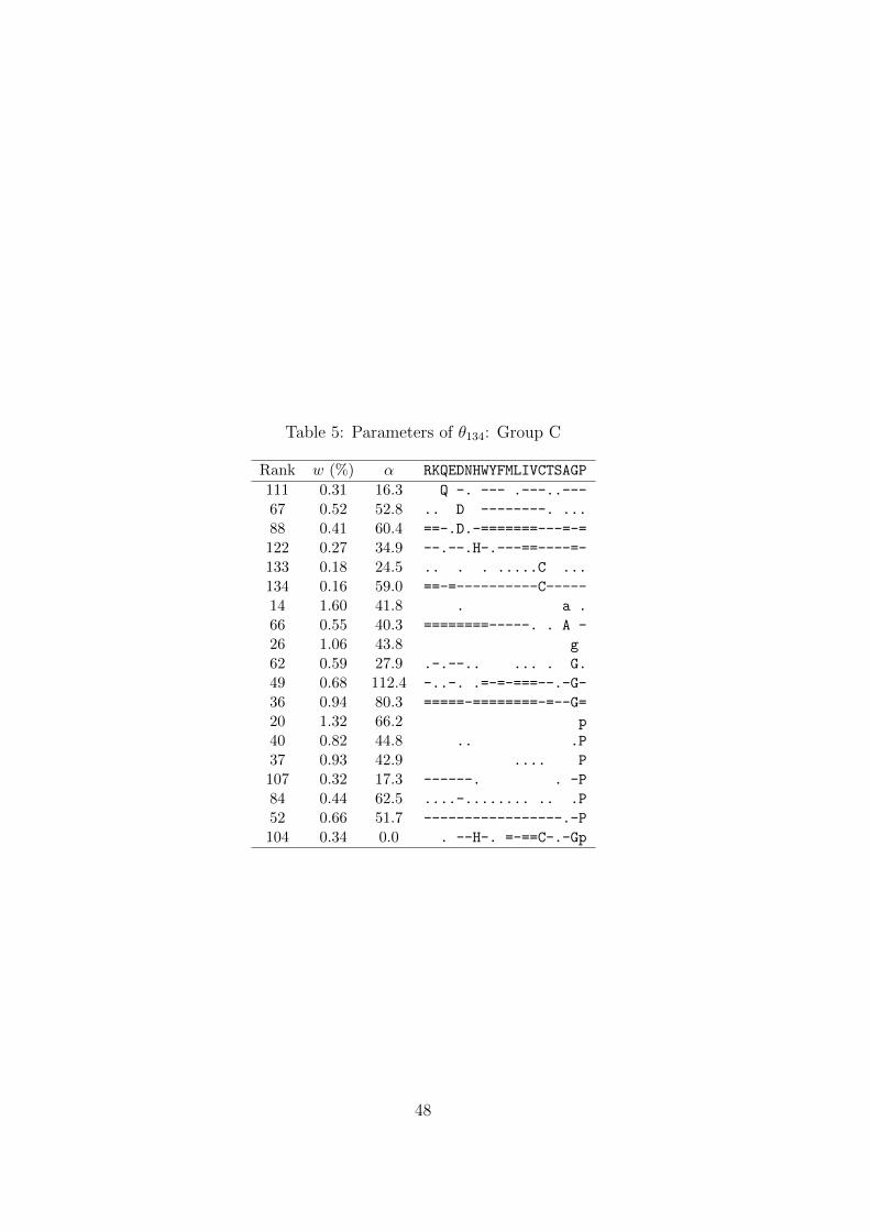
Table 5: Parameters of θ134: Group C
Rank w (%) α RKQEDNHWYFMLIVCTSAGP
111 0.31 16.3 Q -. --- .---..---
67 0.52 52.8 .. D --------. ...
88 0.41 60.4 ==-.D.-=======---=-=
122 0.27 34.9 --.--.H-.---==----=-
133 0.18 24.5 .. . . .....C ...
134 0.16 59.0 ==-=----------C-----
14 1.60 41.8 . a .
66 0.55 40.3 ========-----. . A -
26 1.06 43.8 g
62 0.59 27.9 .-.--.. ... . G.
49 0.68 112.4 -..-. .=-=-===--.-G-
36 0.94 80.3 =====-========-=--G=
20 1.32 66.2 p
40 0.82 44.8 .. .P
37 0.93 42.9 .... P
107 0.32 17.3 ------. . -P
84 0.44 62.5 ....-........ .. .P
52 0.66 51.7 -----------------.-P
104 0.34 0.0 . --H-. =-==C-.-Gp
48


![012#$345678 9 - ChaSen.orgchasen.org/~daiti-m/paper/IBISMLTutorial-NLPU.pdf · usage : um -M mixtures [-e eta] [-g gamma] [-d epsilon] [-I emmax] train model eta = Dirichlet prior](https://img.pdfslide.net/doc/110x75/5be5001c09d3f219598daa3d/012345678-9-daiti-mpaperibismltutorial-nlpupdf-usage-um-m-mixtures.jpg)