Disadvantage and discrimination in self-employment: caste ... · Disadvantage and discrimination in self-employment: caste ... More details about DICCI can be found at . ... Disadvantage

Disadvantage and discrimination in self-employment: castegaps in earnings in Indian small businesses

Ashwini Deshpande . Smriti Sharma

Accepted: 22 October 2015 / Published online: 8 December 2015

� Springer Science+Business Media New York 2015

Abstract Using the 2004–2005 India Human Devel-

opment Survey data, we estimate and decompose the

earnings of household businesses owned by histori-

cally marginalized social groups known as Scheduled

Castes and Tribes (SCSTs) and non-SCSTs across the

earnings distribution. We find clear differences in

characteristics between the two types of businesses

with the former faring significantly worse. The mean

decomposition reveals that as much as 55 % of the

caste earnings gap could be attributed to the unex-

plained component. Quantile regressions suggest that

gaps are higher at lower deciles, providing some

evidence of a sticky floor. Finally, quantile decompo-

sitions reveal that the unexplained component is

greater at the lower and middle deciles than higher,

suggesting that SCST-owned businesses at the lower

and middle end of the conditional earnings distribution

face greater discrimination.

Keywords Caste � Discrimination � Household

business � Earning gaps � Quantile decomposition �India

JEL Classifications J31 � J71 � C21 � O15 �O17 � L26

1 Introduction

Ethnic and racial discrimination in labor markets, as

manifested in wage and occupational attainment gaps,

has been widely examined (e.g., Altonji and Blank

1999; Antecol and Bedard 2004; Atal et al. 2009). In

India too, labor market discrimination against histor-

ically disadvantaged caste groups, i.e., the former

untouchables (Scheduled Castes or SCs) and

marginalized tribal groups (Scheduled Tribes or

STs), is well documented, with SCs and STs earning

significantly lower wages and being allocated to less

prestigious jobs as compared to upper castes, after

controlling for their productive characteristics (Ban-

erjee and Knight 1985; Madheswaran and Attewell

2007; Das and Dutta 2007).1 However, the disadvan-

tage faced by these groups may not be limited merely

to wage employment and could extend to the realm of

self-employment as well. While there is a sizable

literature from the USA that studies racial differences

in entrepreneurship in terms of business creation rates,

survival, employment, profits and net worth (e.g.,

Fairlie 2004, 2006; Ahn 2011; Lofstrom and Bates

A. Deshpande (&)

Department of Economics, Delhi School of Economics,

University of Delhi, Delhi 110007, India

e-mail: [email protected]

S. Sharma

UNU-WIDER, Katajanokanlaituri 6B, 00160 Helsinki,

Finland

e-mail: [email protected]

1 For detailed discussions on caste-based economic discrimi-

nation in India, see Deshpande (2011).

123

Small Bus Econ (2016) 46:325–346

DOI 10.1007/s11187-015-9687-4

http://crossmark.crossref.org/dialog/?doi=10.1007/s11187-015-9687-4&domain=pdf

http://crossmark.crossref.org/dialog/?doi=10.1007/s11187-015-9687-4&domain=pdf

2013), examination of such issues in the Indian context

is relatively recent, due to data constraints.2

Our paper attempts to fill this gap for India, by

assessing caste discrimination in household non-farm

businesses (‘businesses’ hereafter), which has been

possible due to the recent availability of good-quality

earnings data for such businesses. Given the small

scale of operations of these businesses, catering

mostly to customers in the local community, it is

highly plausible that businesses owned by low-caste

owners face discrimination at the hands of customers,

suppliers and lenders, since their caste status is easily

identifiable, unlike in large businesses with complex

ownership and management structures, where observ-

ing the caste of the owners might be less straightfor-

ward. However, discrimination could be directed

toward larger low-caste businesses too: In personal

interviews, rich SC entrepreneurs have discussed their

individual battles with caste discrimination as they

started their businesses.3 There are other ethnographic

accounts as well (Jodhka 2010; Prakash 2010) that

indicate the presence of persistent disadvantage and

discrimination in the self-employment arena, which

forms the motivation for the present study.

To the best of our knowledge, ours is the first paper

to examine caste gaps in earnings from household

businesses for India. We use the India Human

Development Survey data for 2004–2005 and employ

two methodologies for understanding the earnings

structure of businesses: OLS estimation of mean

earnings for businesses owned by SCs and STs and

non-SCST businesses; and quantile regressions for a

distributional analysis to look beyond the mean and to

understand ‘what happens where’ in the earnings

distribution. Correspondingly, we use decomposition

strategies to decompose the earnings gap between

SCST and non-SCST businesses into explained and

unexplained components (with the latter being indica-

tive of discrimination), at the mean and at various

quantiles of the earnings distribution.4

Our main findings are as follows. There are clear

differences in observable characteristics between

SCST and non-SCST businesses. The latter are more

urban, record larger number of total man-hours, have

better educated and richer owners, and are more likely

to have a business in a fixed workplace. These

disparities get reflected in both indicators of business

performance in the data—gross receipts and net

income—such that SCSTs, on average, perform

significantly poorly compared to non-SCSTs. The

Blinder–Oaxaca decomposition reveals that depend-

ing on the specification of variables, assuming that the

non-discriminatory earning structure is that of non-

SCSTs, at least 20 % of the net income gap could be

attributed to the unexplained or the discriminatory

component. Unconditional caste gaps in earnings are

higher at lower percentiles than at the higher per-

centiles. Thus, we find some evidence supporting a

‘sticky floor,’ a phenomenon observed in the context

of gender wage gaps in developing countries (e.g., Chi

and Li 2008; Carrillo et al. 2014). Quantile decompo-

sitions based on our preferred specification reveal that

the unexplained component is significant in the middle

part of the distribution (viz., between the fourth and

eighth deciles), where it hovers around 15 % of the

total gap in earnings.

In addition to contributing to the broader literature

on racial and ethnic disparities in small business

ownership from a developing country perspective, this

paper has significant policy implications, particularly

in the context of the current discourse on ‘Dalit

Capitalism’ in India—inspired by ‘Black Capitalism’

in the USA—by the Dalit Indian Chamber of Com-

merce and Industry (DICCI).5 DICCI believes that

Dalits should enter business and industry sectors as

entrepreneurs and use this route to become ‘job givers,

and not job seekers’ especially for others in their own

community and enhance their wealth, instead of being

dependent on the state for benefits. However, the

majority of Dalit businesses are small, owner-oper-

ated, survivalist household enterprises that do not have2 The Employment–Unemployment Survey conducted by the

National Sample Survey (NSS) collects data on earnings of

salaried employees and casual workers, but not of the self-

employed.3 See, for instance, interviews in Outlook Business, May 2,

2009, p. 25.4 Large Indian data sets such as the NSS and Economic Census

define four broad social groups: Scheduled Castes (SCs),

Scheduled Tribes (STs), Other Backward Classes (OBCs) and

Footnote 4 continued

‘others.’ ‘Others’ is a reasonable approximation of the upper

castes. Even though these large omnibus administrative cate-

gories mask intra-group heterogeneity, it is standard practice to

use these for empirical estimation since data are available only

for these categories.5 SCs use the term Dalit (meaning oppressed) as a term of pride.

More details about DICCI can be found at www.dicci.org.

326 A. Deshpande, S. Sharma

123

http://www.dicci.org

the potential to generate either employment or wealth

(Deshpande and Sharma 2013). Further, our results

indicate that discriminatory tendencies that exist in

labor markets may characterize business operations as

well.

The rest of this paper is organized as follows:

Sect. 2 contains a literature review; Sect. 3 outlines

the methodology; Sect. 4 discusses the data and

descriptive statistics; Sect. 5 presents the results,

while Sect. 6 discusses our findings. Section 7

concludes.

2 Review of related literature

Iyer et al. (2013) and Thorat and Sadana (2009) in

descriptive analyses using Indian Economic Census

data document caste differences in non-agricultural

enterprise ownership and performance.6 They find

SCs and STs to be underrepresented relative to their

population shares. Enterprises owned by SCSTs are

smaller in terms of number of workers, hire mostly

family labor, rely less on external sources of finance

and operate mostly in the unregistered unorganized

sector as compared to enterprises owned by non-

SCSTs. Deshpande and Sharma (2013) examine unit-

level data from two successive censuses of the micro-,

small and medium enterprises (MSME) sector to study

the nature of participation of marginalized groups in

self-employment and found that the MSME sector

exhibits very clear differences along business owners’

caste and gender, in virtually all business

characteristics.

This evidence of systematic differences, however,

does not prove discrimination; all the gaps in perfor-

mance could, in principle, be accounted for by

differences in characteristics of SCST and non-SCST

businesses.7 For example, in the USA, racial dispar-

ities in asset ownership and family background in self-

employment (with blacks being more disadvantaged

than whites) are among the most important factors

leading to differences in business creation and

performance (Dunn and Holtz-Eakin 2000; Hout and

Rosen 2000). However, even after controlling for

differences in characteristics, a significant proportion

of the performance gap remains unexplained and that

could be on account of discrimination or some

unobserved differences in behavior such as ability

and risk aversion or some factors not amenable to

measurement.

Discrimination manifests itself in self-employment

primarily in the form of consumer and credit market

discrimination. For example, Borjas and Bronars

(1989) study consumer discrimination and find that

relative gains of entering self-employment are reduced

for ethnic minorities because they have to compensate

white consumers by lowering prices charged for goods

and services. Coate and Tennyson (1992) study credit

discrimination assuming that lenders are unable to

observe entrepreneurial ability. Individuals from a

group discriminated against in the labor market will

receive less favorable terms in the credit market since

lenders know that for such individuals, the opportunity

cost of entering self-employment is lower, and, thus,

they are willing to take more risks. Such groups will be

charged higher interest rates, thereby reducing the

expected returns from self-employment. Empirical

analyses using data from the USA show that the

probability of loan denials and rates of interest charged

on approved loans is higher for black-owned busi-

nesses than whites (Blanchflower et al. 2003) and

probability of loan renewals is lesser for black- and

Hispanic-owned businesses (Asiedu et al. 2012).

Section 6 discusses the evidence from Prakash

(2010), Jodhka (2010) and Kumar (2013), among

others, to understand possible channels of discrimina-

tion against Dalit businesses in India.

3 Methodology

3.1 Blinder–Oaxaca decomposition framework

We first use the Blinder–Oaxaca method to decom-

pose the mean earnings gap from self-employment

between SCSTs and non-SCSTs into portions

attributable to differences in characteristics (the

explained component or composition effect) and

differences in returns to these endowments (the

unexplained component or coefficients effect) (Blin-

der 1973; Oaxaca 1973). While the unexplained

6 Audretsch et al. (2013) use NSS data to explore the influence

of religious and caste affiliation on occupation choice. They find

SCs and STs to be less likely to be self-employed.7 The fact that SCSTs possess inferior characteristics suggests

some ‘pre-market’ discrimination (Deshpande 2011; Thorat and

Newman 2010).

Disadvantage and discrimination in self-employment 327

123

component can be attributed to discrimination, it is

highly plausible that this residual also includes the

effects of either unmeasurable or unobservable char-

acteristics. All decomposition exercises are subject to

this caveat. However, it is equally true that some pre-

market discrimination affects the formation of char-

acteristics, and thus, the explained component also

embodies the effects of past discrimination. Therefore,

estimates of the unexplained component from decom-

position exercises should not be taken as precise

measurements of ‘true’ discrimination, but as rough

estimates, providing orders of magnitude.

This method involves estimating earnings equa-

tions separately for individuals i of the different

groups g, SCSTs (group s) and non-SCSTs (group n):

wig ¼ Xgi b

g þ ugi ð1Þ

where g = (n, s) denotes the two groups. The depen-

dent variable w is the natural log of earnings. Xi is the

vector of covariates for individual i, which contains

characteristics that would determine earnings. b is the

corresponding vector of coefficients, and u is the

random error term.

The gross difference in earnings between the two

groups can be written as:

G ¼ �Xnb̂n � �Xsb̂s ð2Þ

In order to decompose this gap, some assumptions

have to be made about the earnings structure that

would prevail in the absence of discrimination and

construct counterfactual earnings functions. One

counterfactual could be constructed by assuming that

the non-discriminatory earnings structure is the one

applicable to non-SCSTs.8 In that case, the counter-

factual earnings equation of the SCSTs would be

written as:

wcis ¼ Xs

ibn þ vsi ð3Þ

Adding and subtracting the counterfactual earnings

to Eq. (2), we arrive at:

G ¼ �wn � �ws ¼ �Xn � �Xsð Þb̂n þ �Xs b̂n � b̂s� �

ð4Þ

where the first term on the right-hand side represents

the part of the earnings differential due to differences

in characteristics and the second term represents

differences due to varying returns to the same

characteristics. The second term is the unexplained

component and is considered to be a reflection of

discrimination.

The decomposition is sensitive to the choice of the

non-discriminatory earnings structure, as the two

counterfactuals yield different estimates. To get

around this ‘index number problem,’ one solution is

to use the pooled estimates as the single counterfactual

(Oaxaca and Ransom 1994). Another solution, sug-

gested by Cotton (1988), is to construct the non-

discriminatory earnings structure as a convex linear

combination of the earnings structures of both groups.

3.2 Quantile regression decomposition

framework

Generalizing the traditional Blinder–Oaxaca decom-

position to analyze earnings gaps at different parts of

the earnings distribution, Machado and Mata (2005)

proposed a decomposition method that involves

estimating quantile regressions separately for the two

subgroups and then constructing a counterfactual

using covariates of one group and returns to those

covariates for the other group.

The conditional earnings distribution is estimated

by quantile regressions. The conditional quantile

function Qh (w|X) can be expressed using a linear

specification for each group as follows:

Qh wgjXg

� �¼ XT

i;gbg;h for each h 2 ð0; 1Þ ð5Þ

where g = (n, s) denotes the two groups. w is the

natural log of earnings. Xi is the set of covariates for

individual i, bh are the coefficient vectors that need to

be estimated for the different hth quantiles. The

quantile regression coefficients can be interpreted as

the returns to various characteristics at different

quantiles of the conditional earnings distribution.

Next, Machado and Mata (2005) construct the

counterfactual unconditional earnings distribution

using estimates for the conditional quantile regres-

sions, which consists of the following steps:

1. Generate a random sample of size m from a

uniform distribution U [0,1]

8 One could also construct an alternative counterfactual by

assuming that the non-discriminatory earnings structure is the

one applicable to the SCSTs. However, the counterfactual based

on the non-SCST earnings structure is more intuitively appeal-

ing, as non-SCSTs are not discriminated against on account of

their caste identity.


123

2. For each group, separately estimate m different

quantile regression coefficients

3. Generate a random sample of size m with

replacement from the empirical distribution of

the covariates for each group, Xs,i and Xn,i

4. Generate the counterfactual of interest by mul-

tiplying different combinations of quantile coef-

ficients and distribution of observables between

group s and group n after repeating this last step

m times.

Standard errors are computed using a bootstrapping

technique.

This simulation-based estimator relies on the

generation of a random sample with replacement to

construct the counterfactual unconditional earnings

distribution and comes at the cost of increased

computational time. Melly (2006) proposed a proce-

dure that is less computationally intensive and faster

by integrating the conditional earnings distribution

over the entire range of covariates to generate the

marginal unconditional distribution of log earnings.

This procedure uses all the information contained in

the covariates and makes the estimator more efficient

than the one suggested by Machado and Mata (2005).

The Melly (2006) and Machado and Mata (2005)

decompositions are numerically identical when the

number of simulations in the latter goes to infinity.

We construct a counterfactual for the SCST group

using the characteristics of SCSTs and the earning

structure for non-SCSTs here:

CFsh ¼ XT

s;ibn;h ð6Þ

This yields the following decomposition:

Dh ¼ Qn;h � CFsh

� �þ CFs

h � Qs;h� �

ð7Þ

The first term on the right-hand side represents the

effect of characteristics (explained component) and

the second the effect of returns to characteristics

(coefficients effect or unexplained component).

4 Data and descriptive statistics

4.1 Data

We use the India Human Development Survey (IHDS)

for 2004–2005, which is a nationally representative

data set covering 41,554 households across 1504

villages and 971 urban states in 33 states of India. The

modules of the survey collect data on a wide range of

questions relating to economic activity, income and

consumption expenditure, asset ownership, social

capital, education, health, marriage and fertility, etc.

The survey module on household non-farm busi-

nesses does not identify the primary decision-maker in

the business. However, we can identify specific

members in the household who worked in the business

and the amount of time they spent, in terms of days per

year and hours per day. Using that information, we

assume that the person who has spent maximum

number of hours in the business is the de facto

decision-maker.

We restrict the sample to those states where there

are at least 50 household businesses, leaving us with

22 states.9 We consider only male businesses (i.e.,

where men are the primary decision-makers) in the

main analysis because factors affecting selection into

self-employment vary along lines of gender; addition-

ally, in order to delineate the effect of caste, we need to

hold gender constant, so as not to confound the effect

of overlapping identities.10

The data canvasses information on two measures of

financial performance of the business: net income and

gross receipts. Our primary dependent variable is the

log of net income from the business over the last

12 months. Net income is computed as gross receipts

less hired workers’ wages less cost of materials, rent,

interest on loans, etc. One issue on which the data are

patchy is the use of unpaid family labor in these

businesses, which would affect the calculation of net

income. While some businesses in the data report the

individual components as well as a net income, others

report only the net income. However, our queries with

the IHDS team revealed that when hired labor is not

reported, it cannot be assumed that no labor was

9 These states are: Jammu and Kashmir, Himachal Pradesh,

Punjab, Uttaranchal, Haryana, Delhi, Rajasthan, Uttar Pradesh,

Bihar, Tripura, Assam, West Bengal, Jharkhand, Orissa,

Chhattisgarh, Madhya Pradesh, Gujarat, Maharashtra, Andhra

Pradesh, Karnataka, Kerala and Tamil Nadu.10 In Appendix 2, we report results of the mean decomposition

for the sample of 1099 businesses where the primary decision-

makers are female (SCSTs: 266, non-SCSTs: 833). Since the

total sample of 1099 females is not sufficient to estimate

quantile decompositions with precision, we do not estimate

those. Using the non-SCST coefficients, 68.7 % of the mean

earnings gap is explained using our preferred specification, with

31 % remaining unexplained.


123

actually hired. Thus, data do not allow us to clearly

distinguish between hired and unpaid family labor,

resulting in the inability to estimate ‘true’ net income.

We, thus, use the net income figures in the data as

reported. While expenditure-based indicators have

been found to be more reliable than income-based

measures in developing countries—on account of recall

errors, non-response and deliberate mis-reporting—for

an analysis focusing on enterprise performance, income

is the most appropriate outcome to consider.

As explanatory variables, we use individual-speci-

fic variables such as age, marital status and standard

years of education completed of the decision-maker;

household-specific variables such as wealth (proxied

by asset ownership), rural/urban status, whether

someone close to or within the household is an official

of the village panchayat/nagarpalika/ward committee

and membership in the following: business or profes-

sional group; credit or savings group; caste associa-

tion; development group and agricultural, milk or

other co-operative; and business-specific variables

such as number of family members who worked in the

business, total number of hours put into the business,

work place type and industry type.11 Admittedly,

business-specific variables and some household-speci-

fic variables such as membership in different types of

networks and wealth are potentially endogenous with

respect to business performance. However, as Fortin

et al. (2011) argue, decompositions are accounting

exercises that allow one to quantify the contribution of

factors to the difference in outcome between two

groups without necessarily shedding any light on the

mechanisms explaining the relationship between such

factors and outcomes.

As our sample is limited to only those households

that operate businesses, a potential limitation of our

estimations is that coefficients of earnings regressions

may be biased since individuals and households do not

randomly select into self-employment. Unfortunately,

our data set does not provide us with suitable instru-

ments to correct for selection.

4.2 Descriptive statistics

Table 1 lists the summary statistics for the whole

sample and for the sample of SCST and non-SCST

businesses separately. Of the total 7288 businesses,

1300 are owned by SCSTs (17.8 %) and the remaining

5988 by non-SCSTs (82.2 %).12

In terms of performance, the average net income for

non-SCST businesses (Rs. 45,218) is 1.76 times that

for SCST businesses (Rs. 25,640). A similar pattern

can be seen in the average gross receipts. Figure 1

plots the kernel density distribution of log income for

SCST and non-SCST businesses. The distribution of

incomes of non-SCST businesses lies distinctly to the

right of the SCST businesses.

This large difference in business performance could

be on account of a variety of characteristics, in most of

which there are clear differences between SCSTs and

non-SCSTs. The primary decision-maker is on aver-

age 39 years old, and 86 % of them are married. These

numbers are similar across SCST and non-SCST

decision-makers. However, average years of educa-

tion differ significantly by caste, with 8.3 years for

non-SCSTs and 5.7 years for SCSTs.

There is a distinctly different pattern in the rural–

urban distribution across castes with 33 % of SCST

households and 53 % of non-SCST households being

located in urban areas. There is also disparity in

material standard of living as reflected in asset

ownership, in that out of the 16 assets in the

questionnaire, non-SCSTs own approximately 8,

while SCSTs own around 5.13 We create a wealth

index using principal components analysis and divide

the sample into three groups following Filmer and

Pritchett (2001): those lying in the bottom 40 %

(poor), middle 40 % (middle) and the top 20 % (rich).

By this somewhat arbitrary definition, 65.2 % of

SCST households fall in the poor category, while

34.6 % of non-SCST households are poor. 27.4 and

42.7 % of SCSTs and non-SCSTs, respectively, are in

the middle, and 7.4 % of SCSTs and 22.7 % of non-

SCSTs are rich.

11 Definitions of variables are available in Appendix 1.

12 Since the decomposition methodology is applicable only to

pairs of groups, we club together relatively similar groups, albeit

with intra-group heterogeneity, into two broad dissimilar

groups.13 The IHDS data contain information on the ownership of the

following 16 items (binary variables): cycle/bicycle, sewing

machine, generator set, mixer/grinder, air cooler, motorcycle/

scooter, black and white television, color television, clock/

watch, electric fan, chair or table, cot, telephone, cell phone,

refrigerator and pressure cooker.


123

Table 1 Summary

statistics

Standard errors are reported

in parentheses. Net income

is defined as gross receipts

less hired workers’ wages

less all other expenses such

as costs of materials, rent,

interest on loans, etc

Variable All

enterprises

SCST

enterprises

Non-SCST

enterprises

Outcome variables

Gross receipts (Rs.) 108,015.8

(258,019)

58,804.02

(98,524.46)

118,708.7

(279,809.3)

Net income (Rs.) 41,726.15

(45,158.62)

25,640.14

(32,726.04)

45,218.44

(46,704.93)

Explanatory variables

Individual characteristics

Age (in years) 39.13

(12.43)

38.6

(12.53)

39.25

(12.4)

Married 0.86

(0.34)

0.86

(0.34)

0.86

(0.34)

Years of education 7.79

(4.64)

5.66

(4.57)

8.25

(4.53)

Household characteristics

SCST 17.84

(0.38)

Urban location 0.49

(0.5)

0.33

(0.47)

0.53

(0.5)

Membership in

Business group 0.08

(0.28)

0.06

(0.23)

0.09

(0.29)

Credit or savings group 0.07

(0.26)

0.07

(0.26)

0.07

(0.26)

Caste association 0.14

(0.35)

0.13

(0.33)

0.15

(0.35)

Development group 0.02

(0.14)

0.01

(0.1)

0.02

(0.15)

Co-operative 0.03

(0.18)

0.02

(0.15)

0.04

(0.19)

Village panchayat or ward committee 0.11

(0.31)

0.13

(0.33)

0.11

(0.31)

Business characteristics

Number of family workers 1.39

(0.7)

1.48

(0.8)

1.37

(0.67)

Number of hours 2585.73

(1614.59)

2065.16

(1480.38)

2698.74

(1620.45)

Workplace: home-based 0.25

(0.43)

0.26

(0.44)

0.25

(0.43)

Workplace: other fixed 0.52

(0.5)

0.4

(0.49)

0.55

(0.5)

Workplace: moving 0.23

(0.42)

0.35

(0.48)

0.2

(0.4)


123

We also examine networks since these can affect

the decision to become self-employed, as well as the

prospective success of the business (Allen 2000). In

general, participation in such networks is low. 8 % of

all businesses are members of business or professional

groups with membership of SCST businesses being

below average (5 %). Participation in credit or savings

groups does not differ by caste, covering roughly 7 %

of owners. Membership in caste associations is 14 and

12 % for non-SCST and SCST businesses, respec-

tively. Membership in development groups and co-

operatives is miniscule across the board. In terms of

political networks, 12.5 % of SCSTs have someone in,

or close to, their household who has been an official in

local bodies, while for non-SCSTs, the corresponding

figure is 10.6 %.14 Overall, there is no discernible

pattern in network participation of the two groups in

our data.

These gaps in performance could also be related to

other characteristics, such as (a) the number of family

members who worked in the business: SCST busi-

nesses have greater than average number of family

members working in the business (1.47), as compared

to non-SCST businesses (1.37); and (b) the total

number of hours put in by everyone working in the

business: Non-SCST businesses record 1.3 times more

hours than their SCST counterparts.

In terms of business location, about 25 % of

businesses are home-based, and this proportion does

not differ by caste. 34 % of SCSTs and 20 % of non-

SCSTs have mobile workplaces, while the proportions

of non-SCSTs and SCSTs with fixed workplaces are

55 and 39, respectively. To the extent a fixed

workplace indicates permanency, it suggests that

non-SCST businesses are more stable and less

makeshift.

The most important sector for these businesses is

‘wholesale, retail trade and restaurants and hotels,’

which include activities such as running of ‘kirana’

(neighborhood grocery) stores, other grocery and

general stores, and petty shops. 56 % of non-SCST

businesses and 44.5 % of SCST businesses are

involved in this sector. About 13 % of businesses are

in manufacturing activities, and this proportion does

not vary by caste. The major activities here are

blacksmiths, carpenters and flour mills. About 16 % of

businesses are in the ‘community, social and personal

services’ sector. This includes activities such as

barbers, cycle repair shops and tailoring. These

examples also corroborate our intuition that these

businesses are engaged in low-end activities, and are

more survivalist than entrepreneurial.

Approximately 6.5 % of businesses are in the

‘transport, storage and communication’ sector, with

the proportion being the same across castes. Overall,

only 4 % of businesses are in the primary sector

(agriculture, hunting, forestry and fishing), but 15 %

of SCST businesses are in this sector. Proportions in

‘construction’ and ‘financing, insurance, real estate

and business services’ are small, involving only about

2 % of businesses each. Businesses engaged in

‘mining and quarrying’ and ‘electricity, gas and

water’ sectors are practically non-existent, as

expected, since these highly capital-intensive activi-

ties are not conducive to self-employment.

5 Results

5.1 Earnings function estimates

Table 2 reports the OLS estimates with log income as

the dependent variable, for the pooled sample, and

separately by caste. We present estimates using two

specifications. Specification 1 uses only exogenous

explanatory variables. This includes age and age

squared (as proxies for experience), whether married

or not, years of education, whether urban or not, and

state of residence. Specification 2 is more exhaustive

and also includes potentially endogenous variables. In

Fig. 1 Kernel density of log income

14 This could possibly reflect the operation of the mandatory

22.5 % caste quotas in local bodies for SCSTs.


123

Table 2 OLS estimation: pooled sample and caste-wise

Dependent variable: log income Specification 1 Specification 2

(1) (2) (3) (4) (5) (6)

Pooled SCST Non-SCST Pooled SCST Non-SCST

SCST -0.349***

(0.056)

-0.103***

(0.039)

Age 0.017**

(0.008)

0.039**

(0.016)

0.016*

(0.009)

0.022***

(0.007)

0.039**

(0.016)

0.019**

(0.008)

Age squared/100 -0.017*

(0.009)

-0.038**

(0.018)

-0.016*

(0.010)

-0.024***

(0.008)

-0.043**

(0.018)

-0.021**

(0.009)

Married 0.141**

(0.056)

-0.078

(0.109)

0.185***

(0.059)

0.060

(0.051)

-0.053

(0.129)

0.091*

(0.048)

Years of education 0.055***

(0.004)

0.065***

(0.010)

0.052***

(0.004)

0.012***

(0.004)

0.011

(0.008)

0.013***

(0.004)

Asset ownership 0.150***

(0.009)

0.138***

(0.027)

0.151***

(0.009)

Urban location 0.721***

(0.049)

0.768***

(0.090)

0.707***

(0.051)

0.250***

(0.036)

0.261***

(0.076)

0.252***

(0.039)

Business or professional

group membership

0.158**

(0.063)

0.195

(0.127)

0.160**

(0.070)

Credit or savings group

membership

-0.120**

(0.048)

-0.124

(0.101)

-0.127**

(0.057)

Caste association membership -0.049

(0.060)

-0.075

(0.085)

-0.054

(0.072)

Development group/NGO

membership

0.067

(0.080)

0.535*

(0.295)

0.060

(0.082)

Co-operative membership -0.096

(0.096)

-0.236

(0.236)

-0.095

(0.102)

Village panchayat or

ward committee

-0.048

(0.064)

-0.042

(0.067)

-0.050

(0.081)

Log (number of hours) 0.552***

(0.029)

0.592***

(0.054)

0.530***

(0.031)

Number of workers -0.043*

(0.026)

-0.077

(0.051)

-0.026

(0.028)

Workplace-other fixed 0.267***

(0.049)

0.262***

(0.078)

0.273***

(0.055)

Workplace-moving 0.159***

(0.055)

0.085

(0.087)

0.178***

(0.061)

Constant 9.500***

(0.272)

9.975***

(0.340)

9.413***

(0.303)

5.280***

(0.280)

5.123***

(0.505)

5.507***

(0.319)

Observations 7271 1298 5973 7035 1252 5783

R2 0.304 0.378 0.252 0.514 0.653 0.454

Robust standard errors clustered at the district level are reported in parentheses. State of residence dummy variables is included in

both specifications, whereas specification 2 also adds industry dummy variables

*** Significant at 1 %;** significant at 5 %;* significant at 10 %


123

addition to variables in the first specification, we

include the asset ownership/wealth index, member-

ships in: business or professional groups, credit or

savings groups, caste associations, development

groups, co-operatives, political networks, number of

hours spent by everyone working in the business,

number of family members working in the businesses,

whether workplace is fixed or moving (reference

category is home-based) and industry type.15

The SCST dummy is negative and significant in

both specifications, indicating that ceteris paribus,

belonging to these marginalized groups, is negatively

correlated with income. As expected, earnings have a

quadratic relationship with the decision-maker’s age

such that earnings initially increase with age and start

to decline thereafter. Businesses operated by more

educated owners also perform better indicating that

more years of formal education may be associated

with higher managerial ability and business acumen.

Households owning more assets are able to overcome

liquidity constraints more easily, and we find that

asset-rich households own more profitable businesses.

Businesses in urban locations perform better possibly

due to proximity to markets and easier availability of

information. The number of hours spent working is

positively correlated with income, as expected. Busi-

nesses based on other fixed locations (outside of the

home) and that are mobile are correlated with higher

incomes than home-based businesses.

Pooled regressions impose the restriction that the

returns to included characteristics are the same for the

two caste groups. Since this assumption is not realistic,

particularly in the Indian context, we also report caste-

specific OLS regressions. Caste-specific OLS esti-

mates indicate that some variables—particularly those

related to memberships in business or professional

groups, development groups and credit groups—

correlate in different ways with performance of SCST

and non-SCST businesses.

5.2 Decomposition of the mean earnings gap

The results of the Blinder–Oaxaca decomposition with

log income as the dependent variable are presented in

Table 3.16 Panel A and Panel B of Table 3 display the

decomposition results using specification 1 and spec-

ification 2, respectively. Within each of these panels,

we report results using: coefficients from a pooled

model over both groups as the reference coefficients;

non-SCST coefficients, i.e., how SCST businesses

would fare if they were treated like non-SCST

businesses; and SCST coefficients, i.e., how non-

SCSTs would fare if they were treated like SCSTs.

It is apparent that as more variables are added in

moving from Panel A to Panel B, the explained

proportion increases and the unexplained proportion

decreases significantly. In Panel B, in the presence of

non-SCST coefficients, the unexplained component is

19 %. Using SCST coefficients, we see that the

unexplained proportion is 10.05 %, and for the pooled

model, the corresponding value is 16 %. Following

Banerjee and Knight (1985), we can take the geomet-

ric mean of the estimates based on the SCST

coefficients and non-SCST coefficients to yield a

single estimate of the unexplained component which

amounts to 13.8 %.

Which of the variables contributes the most to the

explained component? The lower panel of Table 3

shows the contribution of selected significant charac-

teristics to the overall explained part of the income

gap. Using the first specification, years of education

contributes 39–42 % of the explained component,

depending on the counterfactual earnings structure.

Urban location also accounts for 37–44 %. However,

in the second specification, the importance of years of

education and urban location declines significantly to

around 5 and 8 %, respectively, and number of hours

and asset ownership emerge as the dominant variables,

each accounting for approximately 30–40 % of the

explained component. Since variables such as years of

education and urban location are generally positively

correlated with asset ownership, it is not surprising

that upon controlling for the latter, the relative

importance of education and location declines.15 As a robustness check, we also estimated three specifica-

tions: one with purely personal characteristics; second with

personal and household characteristics, and third one being the

same as the full specification with all variables. The results,

robust to alternative specifications, are available from the

authors upon request.

16 This is done using the STATA program ‘oaxaca’ (Jann

2008).


123

5.3 Quantile regressions

For quantile regressions, we use the same two

specifications of the earnings function that we used

for the OLS regressions. The average gap in log

incomes of non-SCST-owned and SCST-owned busi-

nesses is 0.75, which corresponds to a gap of 112 % in

raw net incomes of the two types of businesses. This is

instructive, but when we juxtapose this against the log

income gap for the different quantiles, we see that

restricting the analysis to only mean gaps misses a

large part of the bigger picture. Broadly speaking, as

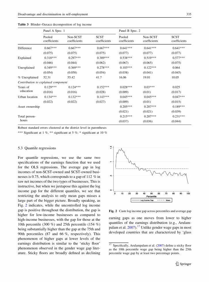
Fig. 2 indicates, while the uncontrolled log income

gap is positive throughout the distribution, the gap is

higher for low-income businesses as compared to

high-income businesses, with the gap for those at the

10th percentile (300 %) and 25th percentile (154 %)

being substantially higher than the gap at the 75th and

90th percentiles (87 and 66 %, respectively). This

phenomenon of higher gaps at lower levels of the

earnings distribution is similar to the ‘sticky floor’

phenomenon observed in the gender wage gap liter-

ature. Sticky floors are broadly defined as declining

earning gaps as one moves from lower to higher

quantiles of the earnings distribution (e.g., Arulam-

palam et al. 2007).17 Unlike gender wage gaps in most

developed countries that are characterized by ‘glass

Table 3 Blinder–Oaxaca decomposition of log income

Panel A Spec. 1 Panel B Spec. 2

Pooled

coefficients

Non-SCST

coefficients

SCST

coefficients

Pooled

coefficients

Non-SCST

coefficients

SCST

coefficients

Difference 0.667***

(0.075)

0.667***

(0.075)

0.667***

(0.075)

0.641***

(0.077)

0.641***

(0.077)

0.641***

(0.077)

Explained 0.318***

(0.046)

0.297***

(0.044)

0.389***

(0.062)

0.538***

(0.067)

0.519***

(0.065)

0.577***

(0.075)

Unexplained 0.349***

(0.054)

0.369***

(0.058)

0.278***

(0.054)

0.103***

(0.038)

0.122***

(0.041)

0.064

(0.045)

% Unexplained 52.31 55.42 41.7 16.06 19.01 10.05

Contribution to explained component

Years of

education

0.129***

(0.016)

0.124***

(0.016)

0.152***

(0.028)

0.028***

(0.009)

0.03***

(0.01)

0.025

(0.017)


(0.022)

0.132***

(0.022)

0.143***

(0.027)

0.045***

(0.009)

0.045***

(0.01)

0.047***

(0.015)


(0.021)

0.207***

(0.021)

0.189***

(0.039)

Total person-

hours

0.215***

(0.037)

0.207***

(0.036)

0.231***

(0.044)

Robust standard errors clustered at the district level in parentheses

*** Significant at 1 %, ** significant at 5 %; * significant at 10 %

Fig. 2 Caste log income gap across percentiles and average gap

17 Specifically, Arulampalam et al. (2007) define a sticky floor

as the 10th percentile wage gap being higher than the 25th

percentile wage gap by at least two percentage points.


123

ceilings’ (i.e., increasing wage gaps as one moves

from lower to higher quantiles), several developing

countries reveal a sticky floor, for instance India

(Khanna 2013; Deshpande et al. 2015), China (Chi and

Li 2008), Bangladesh (Nordman et al. 2015) and

Vietnam (Pham and Reilly 2007). In fact, Carrillo

et al. (2014) find that gender wage gaps in poorer and

more unequal countries exhibit sticky floors, whereas

glass ceilings characterize richer and less unequal

ones, using a sample of 12 Latin American countries.

Tables 4 and 5 report quantile regression results for

the two specifications, respectively, for the pooled

model at the 10th, 25th, 50th, 75th and 90th per-

centiles. The estimates show that controlling for

various characteristics reduces but does not eliminate

the caste gap observed in Fig. 2. In Table 5, even with

the most inclusive specification, the caste dummy

remains negative and significant, but compared to

Table 4, its magnitude is much smaller at each of the

percentiles. The sticky floor no longer prevails as in

Table 4. The caste income gap increases from 10 % at

the 10th percentile to 16 % at the median, declines to

10 % at the 75th percentile and increases again up to

14 % at the 90th percentile.

Results of caste-specific quantile regressions are

reported in Tables 6 and 7. Results from Table 7

indicate that while being married and years of

education are associated positively with income for

non-SCSTs, they are not significant for SCSTs. Being

located in urban areas and number of hours spent in the

business seems to confer greater benefits at the lower

end of the earnings distribution than at the higher end,

for both groups. On the other hand, gains from asset

ownership are mostly increasing across the distribu-

tion for both groups. Returns to other fixed or moving

workplaces appear higher at all percentiles for SCSTs

as compared to non-SCSTs.

5.4 Quantile decompositions of log income gaps

We conduct the quantile decompositions separately

using both specifications.18 Table 8 shows the sum-

mary results with the raw difference, characteristics

effect and coefficients effect at the 10th, 25th, 50th,

75th and 90th percentiles using the non-SCST

Table 4 Quantile regression: specification 1 (pooled sample)

(1) (2) (3) (4) (5) (6)

Mean Q10 Q25 Q50 Q75 Q90

SCST -0.349***

(0.056)

-0.532***

(0.073)

-0.467***

(0.051)

-0.368***

(0.031)

-0.275***

(0.039)

-0.266***

(0.038)

Age 0.017**

(0.008)

0.044***

(0.012)

0.038***

(0.007)

0.033***

(0.012)

0.024***

(0.007)

0.022***

(0.008)

Age squared/100 -0.017*

(0.009)

-0.049***

(0.014)

-0.044***

(0.008)

-0.036***

(0.011)

-0.022***

(0.007)

-0.019**

(0.008)

Married 0.141**

(0.056)

0.132

(0.085)

0.149***

(0.046)

0.110

(0.160)

0.080

(0.053)

0.053

(0.053)


(0.004)

0.052***

(0.005)

0.054***

(0.004)

0.054***

(0.010)

0.059***

(0.003)

0.063***

(0.004)


(0.049)

0.936***

(0.059)

0.743***

(0.037)

0.599***

(0.051)

0.535***

(0.029)

0.491***

(0.030)

Constant 9.500***

(0.272)

7.822***

(0.218)

8.680***

(0.266)

9.503***

(0.179)

10.238***

(0.180)

10.927***

(0.207)

Observations 7271 7271 7271 7271 7271 7271

R2 0.304

Robust standard errors clustered at the district level are reported in parentheses for OLS. Quantile regression standard errors in

parentheses are bootstrapped using 100 replications. State of residence dummy variables included

*** Significant at 1 %; ** significant at 5 %; * significant at 10 %

18 This is done using the STATA program ‘rqdeco’ (Melly

2007).


123

Table 5 Quantile regression: specification 2 (pooled sample)

(1) (2) (3) (4) (5) (6)

Mean Q10 Q25 Q50 Q75 Q90

SCST -0.103***

(0.039)

-0.104**

(0.050)

-0.115***

(0.038)

-0.161***

(0.033)

-0.103***

(0.030)

-0.141***

(0.035)

Age 0.022***

(0.007)

0.052***

(0.010)

0.044***

(0.008)

0.021***

(0.006)

0.017***

(0.005)

0.009

(0.007)

Age squared/100 -0.024***

(0.008)

-0.060***

(0.011)

-0.050***

(0.010)

-0.024***

(0.006)

-0.019***

(0.006)

-0.010

(0.007)

Married 0.060

(0.051)

0.172***

(0.055)

0.091*

(0.053)

0.105**

(0.043)

0.078*

(0.042)

0.091*

(0.050)


(0.004)

0.018***

(0.005)

0.011***

(0.003)

0.012***

(0.003)

0.016***

(0.003)

0.017***

(0.004)


(0.009)

0.118***

(0.011)

0.136***

(0.009)

0.150***

(0.006)

0.170***

(0.006)

0.169***

(0.009)


(0.036)

0.321***

(0.040)

0.268***

(0.027)

0.227***

(0.024)

0.197***

(0.024)

0.189***

(0.032)

Business or professional group membership 0.158**

(0.063)

0.117**

(0.059)

0.060

(0.053)

0.132***

(0.038)

0.095**

(0.043)

0.169***

(0.047)

Credit or savings group membership -0.120**

(0.048)

-0.060

(0.056)

-0.101**

(0.051)

-0.156***

(0.042)

-0.168***

(0.043)

-0.192***

(0.066)

Caste association membership -0.049

(0.060)

-0.023

(0.057)

0.002

(0.050)

0.044

(0.036)

0.058*

(0.034)

0.048

(0.046)

Development group/NGO membership 0.067

(0.080)

0.273**

(0.114)

0.118

(0.091)

0.008

(0.080)

0.041

(0.077)

-0.013

(0.087)

Co-operative membership -0.096

(0.096)

-0.173

(0.106)

-0.118

(0.095)

-0.020

(0.070)

-0.039

(0.074)

0.124*

(0.075)

Village panchayat or ward committee -0.048

(0.064)

-0.060

(0.070)

0.010

(0.037)

-0.009

(0.034)

0.004

(0.037)

-0.026

(0.048)

Log (number of hours) 0.552***

(0.029)

0.686***

(0.030)

0.634***

(0.022)

0.537***

(0.021)

0.416***

(0.023)

0.325***

(0.027)

Number of workers -0.043*

(0.026)

-0.146***

(0.037)

-0.102***

(0.022)

-0.060***

(0.019)

-0.026

(0.022)

0.003

(0.018)

Workplace-other fixed 0.267***

(0.049)

0.320***

(0.049)

0.274***

(0.033)

0.240***

(0.030)

0.125***

(0.031)

0.116***

(0.039)

Workplace-moving 0.159***

(0.055)

0.279***

(0.056)

0.189***

(0.038)

0.163***

(0.036)

0.005

(0.031)

-0.010

(0.045)

Constant 5.280***

(0.280)

2.589***

(0.332)

3.840***

(0.263)

5.517***

(0.234)

7.246***

(0.199)

8.376***

(0.255)

Observations 7035 7035 7035 7035 7035 7035

R2 0.514

Robust standard errors clustered at the district level are reported in parentheses for OLS. Quantile regression standard errors in

parentheses are bootstrapped using 100 replications. State of residence and industry dummy variables included



123

Table

6C

aste

-wis

eq

uan

tile

reg

ress

ion

s:sp

ecifi

cati

on

1

SC

ST

sN

on

-SC

ST

s

(1)

(2)

(3)

(4)

(5)

(6)

(7)

(8)

(9)

(10

)

Q1

0Q

25

Q5

0Q

75

Q9

0Q

10

Q2

5Q

50

Q7

5Q

90

Ag

e0

.08

7*

**

(0.0

28

)

0.0

53

**

(0.0

26

)

0.0

28

*

(0.0

15

)

0.0

45

**

*

(0.0

16

)

0.0

49

**

(0.0

20

)

0.0

37

**

*

(0.0

13

)

0.0

38

**

*

(0.0

09

)

0.0

33

**

*

(0.0

07

)

0.0

23

**

*

(0.0

08

)

0.0

24

**

*

(0.0

08

)

Ag

esq

uar

ed/1

00

-0

.09

7*

**

(0.0

34

)

-0

.05

6*

(0.0

30

)

-0

.03

0*

(0.0

17

)

-0

.04

4*

*

(0.0

19

)

-0

.05

2*

*

(0.0

21

)

-0

.04

2*

**

(0.0

14

)

-0

.04

2*

**

(0.0

10

)

-0

.03

5*

**

(0.0

08

)

-0

.02

1*

*

(0.0

09

)

-0

.02

2*

*

(0.0

08

)

Mar

ried

-0

.14

2

(0.1

65

)

-0

.27

7*

(0.1

61

)

-0

.13

7

(0.1

02

)

-0

.11

8

(0.1

35

)

-0

.27

3*

(0.1

58

)

0.1

89

**

(0.0

86

)

0.1

88

**

*

(0.0

49

)

0.1

41

**

*

(0.0

39

)

0.1

07

*

(0.0

59

)

0.0

79

(0.0

56

)

Yea

rso

fed

uca

tio

n0

.04

8*

**

(0.0

14

)

0.0

46

**

*

(0.0

09

)

0.0

49

**

*

(0.0

09

)

0.0

58

**

*

(0.0

08

)

0.0

65

**

*

(0.0

09

)

0.0

52

**

*

(0.0

05

)

0.0

55

**

*

(0.0

04

)

0.0

54

**

*

(0.0

03

)

0.0

59

**

*

(0.0

03

)

0.0

62

**

*

(0.0

04

)

Urb

anlo

cati

on

0.9

67

**

*

(0.1

36

)

0.8

13

**

*

(0.0

87

)

0.6

18

**

*

(0.0

69

)

0.5

24

**

*

(0.0

61

)

0.3

83

**

*

(0.0

90

)

0.9

21

**

*

(0.0

54

)

0.7

19

**

*

(0.0

30

)

0.5

79

**

*

(0.0

31

)

0.5

28

**

*

(0.0

32

)

0.4

95

**

*

(0.0

41

)

Co

nst

ant

8.2

23

**

*

(0.5

97

)

9.4

51

**

*

(0.5

68

)

10

.66

0*

**

(0.3

75

)

10

.40

5*

**

(0.2

95

)

11

.00

5*

**

(0.4

57

)

7.8

68

**

*

(0.2

70

)

8.4

79

**

*

(0.2

97

)

9.4

03

**

*

(0.1

43

)

10

.10

0*

**

(0.1

86

)

10

.52

5*

**

(0.2

61

)

Ob

serv

atio

ns

12

98

12

98

12

98

12

98

12

98

59

73

59

73

59

73

59

73

59

73

Sta

nd

ard

erro

rsin

par

enth

eses

are

bo

ots

trap

ped

usi

ng

10

0re

pli

cati

on

s.S

tate

of

resi

den

ced

um

my

var

iab

les

incl

ud

ed

**

*S

ign

ifica

nt

at1

%;

**

sig

nifi

can

tat

5%

;*

sig

nifi

can

tat

10

%


123

Table

7C

aste

-wis

eq

uan

tile

reg

ress

ion

s:sp

ecifi

cati

on

2

SC

ST

sN

on

-SC

ST

s

(1)

(2)

(3)

(4)

(5)

(6)

(7)

(8)

(9)

(10

)

Q1

0Q

25

Q5

0Q

75

Q9

0Q

10

Q2

5Q

50

Q7

5Q

90

Ag

e0

.05

1*

*

(0.0

21

)

0.0

51

**

*

(0.0

16

)

0.0

23

(0.0

16

)

0.0

33

**

*

(0.0

13

)

0.0

24

(0.0

18

)

0.0

51

**

*

(0.0

12

)

0.0

41

**

*

(0.0

09

)

0.0

23

**

*

(0.0

05

)

0.0

16

**

*

(0.0

06

)

0.0

10

(0.0

07

)

Ag

esq

uar

ed/1

00

-0

.06

1*

**

(0.0

23

)

-0

.06

2*

**

(0.0

19

)

-0

.02

9

(0.0

18

)

-0

.03

5*

*

(0.0

14

)

-0

.02

4

(0.0

20

)

-0

.05

8*

**

(0.0

13

)

-0

.04

5*

**

(0.0

11

)

-0

.02

6*

**

(0.0

06

)

-0

.01

8*

**

(0.0

07

)

-0

.01

2

(0.0

08

)

Mar

ried

0.1

08

(0.1

44

)

0.0

02

(0.1

12

)

0.0

83

(0.0

76

)

-0

.01

2

(0.1

21

)

-0

.24

3

(0.1

52

)

0.1

76

**

(0.0

73

)

0.1

05

*

(0.0

57

)

0.1

30

**

*

(0.0

38

)

0.1

11

**

*

(0.0

42

)

0.1

23

**

(0.0

59

)

Yea

rso

fed

uca

tio

n0

.02

0

(0.0

14

)

0.0

04

(0.0

09

)

0.0

03

(0.0

06

)

0.0

15

*

(0.0

08

)

0.0

04

(0.0

09

)

0.0

15

**

*

(0.0

05

)

0.0

14

**

*

(0.0

04

)

0.0

12

**

*

(0.0

03

)

0.0

18

**

*

(0.0

03

)

0.0

20

**

*

(0.0

04

)

Ass

eto

wn

ersh

ip0

.12

6*

**

(0.0

38

)

0.1

09

**

*

(0.0

28

)

0.1

44

**

*

(0.0

21

)

0.1

59

**

*

(0.0

19

)

0.1

99

**

*

(0.0

27

)

0.1

19

**

*

(0.0

14

)

0.1

35

**

*

(0.0

09

)

0.1

52

**

*

(0.0

07

)

0.1

69

**

*

(0.0

08

)

0.1

67

**

*

(0.0

09

)

Urb

anlo

cati

on

0.2

11

**

(0.0

97

)

0.2

66

**

*

(0.0

70

)

0.1

65

**

*

(0.0

64

)

0.1

37

**

(0.0

64

)

0.0

28

(0.0

61

)

0.3

52

**

*

(0.0

48

)

0.2

80

**

*

(0.0

30

)

0.2

32

**

*

(0.0

28

)

0.2

13

**

*

(0.0

26

)

0.1

88

**

*

(0.0

44

)

Bu

sin

ess

or

pro

fess

ion

alg

rou

p

mem

ber

ship

-0

.13

4

(0.2

20

)

0.0

04

(0.1

58

)

0.2

59

*

(0.1

48

)

0.1

02

(0.1

00

)

0.0

38

(0.1

60

)

0.1

40

**

(0.0

62

)

0.0

46

(0.0

50

)

0.1

37

**

*

(0.0

46

)

0.1

25

**

*

(0.0

39

)

0.1

78

**

*

(0.0

68

)

Cre

dit

or

sav

ing

sg

rou

pm

emb

ersh

ip0

.15

1

(0.1

81

)

-0

.00

7

(0.0

84

)

-0

.14

7

(0.0

93

)

-0

.21

7*

*

(0.1

10

)

-0

.27

3*

**

(0.0

94

)

-0

.11

2

(0.0

70

)

-0

.11

9*

*

(0.0

49

)

-0

.15

6*

**

(0.0

53

)

-0

.15

9*

**

(0.0

45

)

-0

.18

8*

**

(0.0

65

)

Cas

teas

soci

atio

nm

emb

ersh

ip-

0.1

46

(0.1

74

)

-0

.11

6

(0.0

90

)

-0

.20

4*

*

(0.0

89

)

-0

.11

6

(0.1

04

)

-0

.01

6

(0.1

15

)

-0

.02

1

(0.0

61

)

0.0

37

(0.0

59

)

0.0

73

*

(0.0

37

)

0.0

63

(0.0

41

)

0.0

72

(0.0

49

)

Dev

elo

pm

ent

gro

up

/NG

Om

emb

ersh

ip0

.69

5

(0.5

59

)

0.5

77

*

(0.3

20

)

0.4

77

(0.4

92

)

0.5

22

(0.5

40

)

0.5

23

(0.5

88

)

0.2

41

*

(0.1

26

)

0.1

03

(0.1

10

)

0.0

10

(0.0

74

)

-0

.02

0

(0.0

86

)

-0

.03

9

(0.0

89

)

Co

-op

erat

ive

mem

ber

ship

-0

.30

2

(0.3

13

)

-0

.20

9

(0.1

43

)

-0

.35

6

(0.2

74

)

-0

.03

5

(0.2

23

)

0.0

53

(0.4

54

)

-0

.15

3

(0.1

21

)

-0

.10

0

(0.0

82

)

-0

.03

1

(0.0

79

)

-0

.02

2

(0.0

63

)

0.0

89

(0.0

70

)

Vil

lag

ep

anch

ayat

or

war

dco

mm

itte

e-

0.0

21

(0.1

57

)

0.0

01

(0.1

04

)

-0

.04

9

(0.0

61

)

-0

.13

6

(0.0

83

)

-0

.11

8

(0.1

27

)

-0

.11

3

(0.0

77

)

0.0

11

(0.0

47

)

0.0

20

(0.0

42

)

0.0

47

(0.0

37

)

-0

.00

9

(0.0

50

)

Lo

g(n

um

ber

of

ho

urs

)0

.66

4*

**

(0.0

58

)

0.6

37

**

*

(0.0

36

)

0.6

08

**

*

(0.0

40

)

0.5

13

**

*

(0.0

52

)

0.3

75

**

*

(0.0

54

)

0.6

99

**

*

(0.0

33

)

0.6

02

**

*

(0.0

31

)

0.5

01

**

*

(0.0

23

)

0.3

67

**

*

(0.0

25

)

0.3

01

**

*

(0.0

27

)

Nu

mb

ero

fw

ork

ers

-0

.18

7*

(0.1

01

)

-0

.02

7

(0.0

56

)

-0

.09

0*

*

(0.0

40

)

-0

.01

1

(0.0

47

)

-0

.01

7

(0.0

45

)

-0

.15

8*

**

(0.0

35

)

-0

.08

3*

**

(0.0

24

)

-0

.03

8*

(0.0

20

)

0.0

01

(0.0

23

)

0.0

10

(0.0

21

)

Wo

rkp

lace

-oth

erfi

xed

0.3

63

**

*

(0.1

39

)

0.2

91

**

*

(0.0

74

)

0.3

55

**

*

(0.0

95

)

0.2

33

**

*

(0.0

83

)

0.1

82

**

(0.0

88

)

0.3

08

**

*

(0.0

50

)

0.2

76

**

*

(0.0

32

)

0.2

33

**

*

(0.0

34

)

0.1

17

**

*

(0.0

35

)

0.1

38

**

*

(0.0

45

)


123

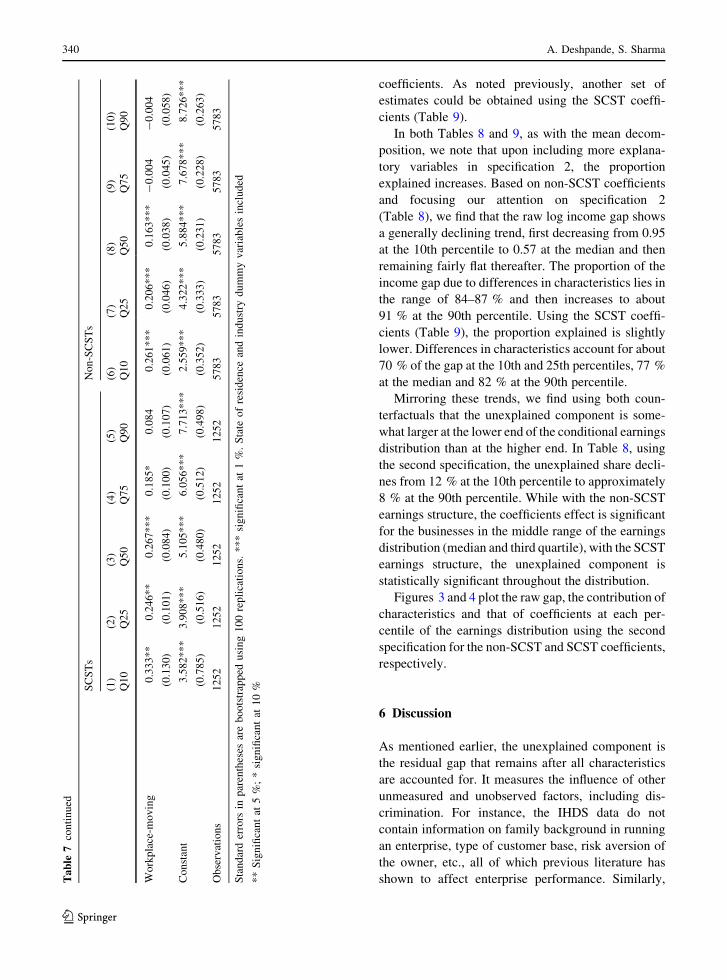
coefficients. As noted previously, another set of

estimates could be obtained using the SCST coeffi-

cients (Table 9).

In both Tables 8 and 9, as with the mean decom-

position, we note that upon including more explana-

tory variables in specification 2, the proportion

explained increases. Based on non-SCST coefficients

and focusing our attention on specification 2

(Table 8), we find that the raw log income gap shows

a generally declining trend, first decreasing from 0.95

at the 10th percentile to 0.57 at the median and then

remaining fairly flat thereafter. The proportion of the

income gap due to differences in characteristics lies in

the range of 84–87 % and then increases to about

91 % at the 90th percentile. Using the SCST coeffi-

cients (Table 9), the proportion explained is slightly

lower. Differences in characteristics account for about

70 % of the gap at the 10th and 25th percentiles, 77 %

at the median and 82 % at the 90th percentile.

Mirroring these trends, we find using both coun-

terfactuals that the unexplained component is some-

what larger at the lower end of the conditional earnings

distribution than at the higher end. In Table 8, using

the second specification, the unexplained share decli-

nes from 12 % at the 10th percentile to approximately

8 % at the 90th percentile. While with the non-SCST

earnings structure, the coefficients effect is significant

for the businesses in the middle range of the earnings

distribution (median and third quartile), with the SCST

earnings structure, the unexplained component is

statistically significant throughout the distribution.

Figures 3 and 4 plot the raw gap, the contribution of

characteristics and that of coefficients at each per-

centile of the earnings distribution using the second

specification for the non-SCST and SCST coefficients,

respectively.

6 Discussion

As mentioned earlier, the unexplained component is

the residual gap that remains after all characteristics

are accounted for. It measures the influence of other

unmeasured and unobserved factors, including dis-

crimination. For instance, the IHDS data do not

contain information on family background in running

an enterprise, type of customer base, risk aversion of

the owner, etc., all of which previous literature has

shown to affect enterprise performance. Similarly,Table

7co

nti

nu

ed

SC

ST

sN

on

-SC

ST

s

(1)

(2)

(3)

(4)

(5)

(6)

(7)

(8)

(9)

(10

)

Q1

0Q

25

Q5

0Q

75

Q9

0Q

10

Q2

5Q

50

Q7

5Q

90

Wo

rkp

lace

-mo

vin

g0

.33

3*

*

(0.1

30

)

0.2

46

**

(0.1

01

)

0.2

67

**

*

(0.0

84

)

0.1

85

*

(0.1

00

)

0.0

84

(0.1

07

)

0.2

61

**

*

(0.0

61

)

0.2

06

**

*

(0.0

46

)

0.1

63

**

*

(0.0

38

)

-0

.00

4

(0.0

45

)

-0

.00

4

(0.0

58

)

Co

nst

ant

3.5

82

**

*

(0.7

85

)

3.9

08

**

*

(0.5

16

)

5.1

05

**

*

(0.4

80

)

6.0

56

**

*

(0.5

12

)

7.7

13

**

*

(0.4

98

)

2.5

59

**

*

(0.3

52

)

4.3

22

**

*

(0.3

33

)

5.8

84

**

*

(0.2

31

)

7.6

78

**

*

(0.2

28

)

8.7

26

**

*

(0.2

63

)

Ob

serv

atio

ns

12

52

12

52

12

52

12

52

12

52

57

83

57

83

57

83

57

83

57

83

Sta

nd

ard

erro

rsin

par

enth

eses

are

bo

ots

trap

ped

usi

ng

10

0re

pli

cati

on

s.*

**

sig

nifi

can

tat

1%

.S

tate

of

resi

den

cean

din

du

stry

du

mm

yv

aria

ble

sin

clud

ed

**

Sig

nifi

can

tat

5%

;*

sig

nifi

can

tat

10

%


123

there are characteristics such as ability or motivation,

which cannot be measured but can affect the earnings

gap. Similarly, as noted earlier, the explained compo-

nent could include pre-market discrimination.

While we cannot test empirically the channels

through which discrimination manifests itself, there

exist studies that qualitatively document the presence

of active discrimination against SCST businesses.

Prakash (2010) in his 2006–2007 survey of 90 Dalit

businesses in 13 districts spread across 6 states in India

reports difficulty in obtaining initial formal credit in

order to set up an enterprise, resulting in informal

loans being taken at high interest rates. The ones who

did successfully obtain institutional credit were those

in partnerships with upper castes or had local political

contacts that facilitated loan approvals. Kumar (2013)

using data from the 2002–2003 All-India Debt and

Investment Survey finds that public sector banks

Table 8 Quantile decompositions of log income (non-SCST coefficients)

Decile Panel A Spec. 1 Panel B Spec. 2

Col. 1 difference Col. 2

characteristics

Col 3. coefficients Col. 4 difference Col. 5

characteristics

Col. 6 coefficients

10 0.999***

(0.045)

0.539***

(0.093)

0.460***

(0.098)

0.949***

(0.043)

0.829***

(0.062)

0.12

(0.096)

25 0.765***

(0.024)

0.394***

(0.059)

0.371***

(0.063)

0.713***

(0.025)

0.615***

(0.043)

0.098

(0.069)

50 0.604***

(0.017)

0.310***

(0.046)

0.294***

(0.042)

0.568***

(0.018)

0.479***

(0.038)

0.089*

(0.052)

75 0.548***

(0.016)

0.321***

(0.044)

0.227***

(0.036)

0.554***

(0.019)

0.473***

(0.042)

0.081*

(0.042)

90 0.546***

(0.019)

0.315***

(0.052)

0.231***

(0.045)

0.569***

(0.021)

0.522***

(0.049)

0.047

(0.051)

Standard errors in parentheses are based on bootstrapping with 100 replications


Table 9 Quantile decompositions of log income (SCST coefficients)

Decile Panel A Spec. 1 Panel B Spec. 2

Col. 1 difference Col. 2

characteristics

Col 3. coefficients Col. 4 difference Col. 5

characteristics

Col. 6 coefficients

10 0.999***

(0.098)

0.25***

(0.054)

0.749***

(0.045)

0.949***

(0.096)

0.663***

(0.077)

0.286***

(0.043)

25 0.765***

(0.063)

0.277***

(0.037)

0.488***

(0.024)

0.713***

(0.069)

0.491***

(0.049)

0.222***

(0.025)

50 0.604***

(0.042)

0.304***

(0.028)

0.3***

(0.017)

0.568***

(0.052)

0.44***

(0.035)

0.128***

(0.018)

75 0.548***

(0.036)

0.303***

(0.026)

0.245***

(0.016)

0.554***

(0.042)

0.467***

(0.034)

0.087***

(0.019)

90 0.546***

(0.045)

0.296***

(0.028)

0.25***

(0.019)

0.569***

(0.051)

0.469***

(0.031)

0.10***

(0.021)

Standard errors in parentheses are based on bootstrapping with 100 replications



123

operating in areas with more upper castes tend to

discriminate more against low-caste loan applicants.

Prakash (2010) also cites Dalit entrepreneurs who

reported often charging less for their products than

their upper-caste peers so that customers ‘forget’ their

castes. Jodhka (2010) through detailed interviews with

Dalit entrepreneurs in two towns in northwest India

finds that caste works as a direct and indirect barrier in

the successful running of their businesses. Most of

them report difficulties on account of their Dalit

identity in mobilizing finance and getting a space to

start their enterprise. A majority of them felt that their

caste identity was perceived as more important than

their professional identity, which led to them being

seen as ‘odd actors’ in the local community.

Another unobserved factor that could constrain

enterprise performance is geographical segregation.

Residential segregation is still prevalent in India with

Dalits living in their own segregated neighborhoods. If

the main customer base of SCST enterprises is their

own community—and given that SCSTs are on

average poorer and have lower purchasing power—

they may have to keep their prices low in order to cater

to members of their own group. For example, Clark

and Drinkwater (2000) explain that ethnic enclaves

can be a source of advantage or disadvantage. While

on the one hand, a concentration of co-ethnics

provides a captive market for producing ethnic goods

that hold particular appeal for the community, on the

other hand, if the ethnic group is poor, then businesses

setup by members of these groups may actually

languish.

7 Conclusion

In this paper, our objective has been to assess the

presence of caste-based discrimination in small

household businesses using the large-scale nationally

representative India Human Development Survey of

2004–2005. Our results show that SCST businesses

fare significantly worse in terms of owner’s education,

household economic status and business characteris-

tics, as compared to their non-SCST counterparts.

Using the non-SCST counterfactual earnings struc-

ture, at least 20 % of the mean earnings gap between

businesses owned by SCSTs and non-SCSTs cannot

be explained by differences in characteristics. Further,

we find that there is substantial heterogeneity in raw

earnings gaps across the earnings distribution reveal-

ing a sticky floor, thereby necessitating the use of

quantile regression-based decomposition methods.

These indicate that the proportion of the earnings

gap on account of differences in characteristics is

generally increasing in the higher deciles of the

conditional earnings distribution.

This paper focuses on one part of the IHDS data set,

viz., data related to household non-farm business,

where we see clear evidence of caste-based disparities

in earnings and other business characteristics, as well

as the existence of discrimination. Desai and Dubey’s

Fig. 3 Quantile decomposition of log income gap: non-SCST

coefficients

Fig. 4 Quantile decomposition of log income gap: SCST

coefficients


123

(2011) analysis based on the entire IHDS data set

suggests that our findings fit into the larger pattern of

persistence of caste inequalities, which results in

inequalities in opportunities as well as inequalities in

outcomes. They find an increase in civic and political

participation by marginalized groups, but also docu-

ment how economic and educational disparities con-

tinue to flourish.

In addition to being the first to examine this

question for India, this paper’s findings confirm

patterns that have been observed in the context of

racial and ethnic differences in entrepreneurship in

other countries such as the USA and UK. However,

unlike the USA, for instance, where a number of

migrant groups such as the Koreans and Japanese have

used self-employment as a way to achieve upward

economic and social mobility that does not appear to

be the case for India, as suggested by our findings and

also those in Iyer et al. (2013) and Deshpande and

Sharma (2013). This also suggests that the exuberance

surrounding Dalit Capitalism may be somewhat

misplaced since the reality of most SC and ST

businesses is in stark contrast to the success of a few

Dalit billionaires.

The simultaneous existence of discrimination

against SCs and STs in self-employment and wage

employment presents serious challenges for public

policy, further complicated by the existence of ‘pre-

market’ discrimination for Dalits which results in

lower and poorer quality of educational and skill

attainment. While caste-based job quotas in India

target public sector-salaried employment, that may not

be the appropriate instrument to tackle discrimination

faced by the self-employed. One such recent move is a

2012 public procurement policy for micro- and small

enterprises (MSE) that mandates 4 % of government

procurement to be from MSEs owned by SCs and STs.

Other multi-pronged measures, based on more

research, need to be devised that would tackle

discrimination in both spheres. For instance, looking

at the entrepreneurial success of migrant groups in

countries such as the USA and UK indicates that

Fairlie’s (2006) suggestion of stimulating business

creation in sectors with high growth potential (e.g.,

construction, wholesale trade and business service)

might be one effective element of public policy for

promoting job creation and increasing earnings,

especially in areas where marginalized groups are

concentrated.

A larger question is the relationship between

earnings and wealth, and whether an increase in

earnings (from businesses and elsewhere) is sufficient

to close the wealth gap between communities. Barsky

et al. (2002) find that roughly two-thirds of the mean

difference in wealth between blacks and whites in the

USA can be explained by differences in earnings from

all sources, which suggests that substantial wealth gaps

remain even after controlling for earning differences.

Whether an increase in business ownership by SCs and

STs translates into narrowing wealth gaps would have

to be the subject matter of a future exercise.

Acknowledgments We are grateful to Deepti Goel and two

anonymous referees for detailed comments; to Shantanu Khanna

for discussions on the quantile regression decomposition

methodology; and to seminar participants at Delhi School of

Economics, Brown University, New Delhi office of the World

Bank, UNU-WIDER, Nordic Conference on Development

Economics 2014, IEA-World Bank Roundtable on Shared

Prosperity, and the IHDS-NCAER 2014 conference on ‘Human

Development in India: evidence from IHDS’ where earlier

versions of the paper were presented, for useful comments. We

are responsible for all remaining errors and omissions.

Compliance with ethical standards

Conflict of interest The authors declare that they have no

conflict of interest.

Appendix 1

In order to canvass data on non-farm businesses, the

survey explicitly asks ‘Does anybody in this

household run their own business, however big or

small? Does anybody make something for sale, such as

cloth or some food like pickles? Or does anybody sell

something in a market or to customers of any sort? Or

does anybody provide a service to others for a price,

either a skilled service like a doctor or an unskilled

service like a barber?’

1. Net income: gross receipts less hired workers’

wages less all other expenses such as costs of

materials, rent, interest on loans, etc.


123

2. Age: in years (of the de facto decision-maker)

3. Marital status: equals 1 if married, 0 otherwise

(of the de facto decision-maker)

4. Years of education: standard number of years of

education completed (of the de facto decision-

maker)

5. Urban: equals 1 if household is in an urban area,

0 otherwise

6. Business or professional group membership:

equals 1 if the household is a member, 0

otherwise

7. Credit or savings group membership: equals 1 if

the household is a member, 0 otherwise

8. Caste association membership: equals 1 if the

household is a member, 0 otherwise

9. Development group/NGO membership: equals 1

if the household is a member, 0 otherwise

10. Co-operative membership: equals 1 if the house-

hold is a member, 0 otherwise

11. Village panchayat or ward committee: equals 1 if

someone in, or close to the household is a

member, 0 otherwise

12. Total number of hours: total number of hours

spent in the business by all household members

involved in the business

13. Number of workers: number of household

members that worked in the business

14. Workplace type: dummy variables for each of the

three categories—home; other fixed place; other

moving place

15. Industry type (NIC-1987): dummy variables for

each of the nine categories—agriculture, hunting,

forestry, fishing; mining and quarrying; manu-

facturing; electricity, gas and water; construc-

tion; wholesale trade, retail trade, restaurants and

hotels; transport, storage and communication;

finance, insurance, real estate and business ser-

vices; community, social and personal services.

16. State: dummy variables for each of the 22

states—Jammu and Kashmir, Himachal Pradesh,

Punjab, Uttaranchal, Haryana, Delhi, Rajasthan,

Uttar Pradesh, Bihar, Tripura, Assam, West

Bengal, Jharkhand, Orissa, Chhattisgarh, Mad-

hya Pradesh, Gujarat, Maharashtra, Andhra

Pradesh, Karnataka, Kerala and Tamil Nadu.

Appendix 2

See Table 10.

Table 10 Blinder–Oaxaca decomposition of log income using the sample of female-run businesses

Panel A Spec. 1 Panel B Spec. 2

Pooled

coefficients

Non-SCST

coefficients

SCST

coefficients

Pooled

coefficients

Non-SCST

coefficients

SCST

coefficients

Difference 0.525***

(0.131)

0.525***

(0.131)

0.525***

(0.131)

0.529***

(0.134)

0.529***

(0.134)

0.529***

(0.134)

Explained 0.296***

(0.072)

0.281***

(0.074)

0.349***

(0.097)

0.364***

(0.11)

0.364***

(0.11)

0.401***

(0.132)

Unexplained 0.229**

(0.116)

0.244**

(0.119)

0.176

(0.12)

0.165*

(0.088)

0.165*

(0.091)

0.128

(0.111)

% Unexplained 43.54 46.41 33.59 31.16 31.28 24.19

Observations 1073 1039

Robust standard errors clustered at the district level in parentheses



123

References

Ahn, T. (2011). Racial differences in self-employment exits.

Small Business Economics, 36, 169–186.

Allen, W. D. (2000). Social networks and self-employment.

Journal of Socio-Economics, 29, 487–501.

Altonji, J. G., & Blank, R. M. (1999). Race and gender in the

labor market. In O. Ashenfelter & D. Card (Eds.), Hand-

book of labor economics (1st ed., Vol. 3, pp. 3143–3259).

Amsterdam: Elsevier.

Antecol, H., & Bedard, K. (2004). The racial wage gap: The

importance of labor force attachment differences across

Black, Mexican, and White Men. Journal of Human

Resources, 39(2), 564–583.

Arulampalam, W., Booth, A. L., & Bryan, M. L. (2007). Is there

a glass ceiling over Europe? Exploring the gender pay gap

across the wage distribution. Industrial and Labor Rela-

tions Review, 60(2), 163–186.

Asiedu, E., Freeman, J. A., & Nti-Addae, A. (2012). Access to

credit by small businesses: How relevant and race, eth-

nicity and gender. American Economic Review: Papers

and Proceedings, 102(3), 532–537.

Atal, J. P., Nopo, H., & Winder, N. (2009). New century, old

disparities gender and ethnic wage gaps in Latin America.

IDB Working Paper No. 109.

Audretsch, D. B., Bonte, W., & Tamvada, J. P. (2013). Religion,

social class, and entrepreneurial choice. Journal of Busi-

ness Venturing, 28, 774–789.

Banerjee, B., & Knight, J. B. (1985). Caste in Indian urban

labour market. Journal of Development Economics, 17,

277–307.

Barsky, R., Bound, J., Charles, K. K., & Lupton, J. P. (2002).

Accounting for the black–white wealth gap: A nonpara-

metric approach. Journal of the American Statistical

Association, 97, 663–673.

Blanchflower, D. G., Levine, P. B., & Zimmerman, D. J. (2003).

Discrimination in the small-business credit market. Review

of Economics and Statistics, 85(4), 930–943.

Blinder, A. S. (1973). Wage discrimination: Reduced form and

structural estimates. Journal of Human Resources, 8,

436–455.

Borjas, G., & Bronars, S. (1989). Consumer discrimination and

self-employment. Journal of Political Economy, 97,

581–605.

Carrillo, P., Gandelman, N., & Robano, V. (2014). Sticky floors

and glass ceilings in Latin America. Journal of Economic

Inequality, 12(3), 339–361.

Chi, W., & Li, B. (2008). Glass ceiling or sticky floor? Exam-

ining the gender earnings differential across the earnings

distribution in urban China, 1987–2004. Journal of Com-

parative Economics, 36(2), 243–263.

Clark, K., & Drinkwater, S. (2000). Pushed out or pulled in?

Self-employment among ethnic minorities in England and

Wales. Labour Economics, 7, 603–628.

Coate, S., & Tennyson, S. (1992). Labor market discrimination,

imperfect information and self-employment. Oxford Eco-

nomic Papers, 44, 272–288.

Cotton, J. (1988). On the decomposition of wage differentials.

Review of Economics and Statistics, 70, 236–243.

Das, M. B., & Dutta, P. (2007). Does caste matter for wages in

the Indian labour market?. Washington, DC, USA: The

World Bank.

Desai, S., & Dubey, A. (2011). Caste in 21st century India:

Competing narratives. Economic and Political Weekly,

XLVI(11), 40–49.

Deshpande, A. (2011). The grammar of caste: Economic dis-

crimination in con-temporary India. New Delhi: OxfordUniversity Press.

Deshpande, A., Goel, D., & Khanna, S. (2015). Bad karma or

discrimination? Male–female wage gaps among salaried

workers in India. Centre for Development Economics

Working Paper 243, Delhi School of Economics.

Deshpande, A., & Sharma, S. (2013). Entrepreneurship or sur-

vival? Caste and gender of small business in India. Eco-

nomic and Political Weekly, XLVIII(28), 38–49.

Dunn, T. A., & Holtz-Eakin, D. J. (2000). Financial capital,

human capital, and the transition to self-employment:

Evidence from intergenerational links. Journal of Labor

Economics, 18(2), 282–305.

Fairlie, R. (2004). Racial trends in ethnic and racial business

ownership. Small Business Economics, 23, 203–218.

Fairlie, R. (2006). Entrepreneurship among disadvantaged

groups: An analysis of the dynamics of self-employment

by gender, race and education. In Simon C. Parker, Zoltan

J. Acs, & David R. Audretsch (Eds.), International hand-

book series on en-trepreneurship (Vol. 2). New York:

Springer.

Filmer, D., & Pritchett, L. (2001). Estimating wealth effect

without expenditure data-or tears: An application to edu-

cational enrollments in states of India. Demography, 38,

115–132.

Fortin, N., Lemiuex, T., & Firpo, S. (2011). Decomposition

methods in economics. In Orley Ashenfelter & David Card

(Eds.), Handbook of labor economics (Vol. 4a). Amster-

dam: Elsevier.

Hout, M., & Rosen, H. (2000). Self-employment, family back-

ground, and race. Journal of Human Resources, 35(4),

670–692.

Iyer, L., Khanna, T., & Varshney, A. (2013). Caste and

entrepreneurship in India. Economic and Political Weekly,

XLVIII(6), 52–60.

Jann, B. (2008). The Blinder–Oaxaca decomposition for linear

regression models. STATA Journal, 8(4), 453–479.

Jodhka, S. (2010). Dalits in business: Self-employed Scheduled

Castes in Northwest India. Indian Institute of Dalit Studies

Working Paper, 4(2).

Karunakaran, N. (2009). Bite the caste bullet. Outlook Business,

May 2.

Khanna, S. (2013). Gender wage discrimination in India: glass

ceiling or sticky floor. Centre for Development Economics

Working Paper 214, Delhi School of Economics.

Kumar, S. M. (2013). Does access to formal agricultural credit

depend on caste? World Development, 43, 315–328.

Lofstrom, M., & Bates, T. (2013). African Americans’ pursuit of

self-employment. Small Business Economics, 40, 73–86.

Machado, J., & Mata, J. (2005). Counterfactual decomposition

of changes in wage distributions using quantile regression.

Journal of Applied Econometrics, 20, 445–465.


123

Madheswaran, S., & Attewell, P. (2007). Caste discrimination in

the Indian urban labour market: Evidence from the national

sample survey. Economic and Political Weekly,

4146–4153.

Melly, B. (2006). Estimation of counterfactual distributions

using quantile regression. Review of Labor Economics, 68,

543–572.

Melly, B. (2007). RQDECO: A stata module to decompose

differences in distribution. Unpublished manuscript,

University of St. Gallen.

Nordman, C. J., Sarr, L., & Sharma, S. (2015). Cognitive, non-

cognitive skills and gender wage gaps: Evidence from

linked employer–employee data in Bangladesh, IZA Dis-

cussion Paper No. 9132.

Oaxaca, R. (1973). Male–female wage differentials in urban

labor markets. International Economic Review, 14,

693–709.

Oaxaca, R., & Ransom, M. (1994). On discrimination and the

decomposition of wage differentials. Journal of Econo-

metrics, 61(1), 5–21.

Pham, T., & Reilly, B. (2007). The gender pay gap in Vietnam:

1993–2002: A quantile regression approach. Journal of

Asian Economics, 18(5), 775–808.

Prakash, A. (2010). Dalit entrepreneurs in middle India. In

Barbara Harriss-White & Judith Heyer (Eds.), The com-

parative political economy of development Africa and

South Asia. London: Routledge.

Thorat, S., & Newman, K. (Eds.). (2010). Blocked by caste:

Economic discrimination in modern India. New Delhi:

Oxford University Press.

Thorat, S., & Sadana, N. (2009). Caste and ownership of private

enterprises. Economic and Political Weekly, XLIV(23),

13–16.


123

Documents

Disadvantage and discrimination in self-employment: caste ... · Disadvantage and discrimination in self-employment: caste ... More details about DICCI can be found at . ... Disadvantage