DISAPPEARING ROUTINE JOBS: NATIONAL …workers towards non-employment. Quantitatively, we find that advances in automation technology on their own account for a relatively small portion

NBER WORKING PAPER SERIES

DISAPPEARING ROUTINE JOBS:WHO, HOW, AND WHY?

Guido Matias CortesNir JaimovichHenry E. Siu

Working Paper 22918http://www.nber.org/papers/w22918

NATIONAL BUREAU OF ECONOMIC RESEARCH1050 Massachusetts Avenue

Cambridge, MA 02138December 2016

We thank David Dorn, Richard Rogerson, and numerous seminar and workshop participants for helpful comments. Siu thanks the Social Sciences and Humanities Research Council of Canada for support. The views expressed herein are those of the authors and do not necessarily reflect the views of the National Bureau of Economic Research.

NBER working papers are circulated for discussion and comment purposes. They have not been peer-reviewed or been subject to the review by the NBER Board of Directors that accompanies official NBER publications.

© 2016 by Guido Matias Cortes, Nir Jaimovich, and Henry E. Siu. All rights reserved. Short sections of text, not to exceed two paragraphs, may be quoted without explicit permission provided that full credit, including © notice, is given to the source.

Disappearing Routine Jobs: Who, How, and Why?Guido Matias Cortes, Nir Jaimovich, and Henry E. SiuNBER Working Paper No. 22918December 2016JEL No. E0,J0

ABSTRACT

We study the deterioration of employment in middle-wage, routine occupations in the United States in the last 35 years. The decline is primarily driven by changes in the propensity to work in routine jobs for individuals from a small set of demographic groups. These same groups account for a substantial fraction of both the increase in non-employment and employment in low-wage, non-routine manual occupations observed during the same time period. We analyze a general neoclassical model of the labor market featuring endogenous participation and occupation choice. We show that in response to an increase in automation technology, the model embodies an important tradeoff between reallocating employment across occupations and reallocation of workers towards non-employment. Quantitatively, we find that advances in automation technology on their own account for a relatively small portion of the joint decline in routine employment and associated rise in non-routine manual employment and non-employment.

Guido Matias CortesEconomics - School of Social SciencesArthur Lewis BuildingManchester, United Kingdom, M13 [email protected]

Nir JaimovichDepartment of Finance and Business EconomicsMarshall Business SchoolUniversity of Southern CaliforniaLos Angeles, CA 90089-0804and [email protected]

Henry E. SiuVancouver School of EconomicsUniversity of British Columbia6000 Iona DriveVancouver, BC V6T 1L4CANADAand [email protected]

1 Introduction

In the past thirty-five years, the US economy has seen a sharp drop in the fraction of the

population employed in middle-skilled occupations. This employment loss is linked to the

disappearance of “routine” occupations—those focused on a relatively narrow set of job

tasks that can be performed by following a well-defined set of instructions and procedures.

This fall in per capita routine employment is a principal factor in the increasing polarization

of the labor market, as employment shares have shifted toward the top and bottom tails of

the occupational wage distribution. Autor, Levy, and Murnane (2003) and the subsequent

literature suggest that job polarization is due to progress in automation technologies that

substitute for labor in routine tasks.

In spite of the growing literature on polarization, relatively little is known regarding the

process by which routine occupations have declined. This is true with respect to who the

loss of routine job opportunities is affecting most acutely, and how they have adjusted in

terms of employment and occupational outcomes.1 And though the number of studies is

growing, the quantitative role of progress in automation technology in the aggregate decline

of routine employment is also unresolved.2 This paper contributes to these open questions.

In Section 2, we study the proximate empirical causes of the decline in per capita

employment in routine occupations. In an accounting sense, roughly one-third of the fall

observed in the past four decades is due to demographic compositional change within the US

population. The more important factor is a sharp change in the propensity of individuals

of given demographic characteristics to work in routine jobs. Crucially, these composition

and propensity effects are strongest for a relatively small set of demographic groups. As a

result, the vast majority of the fall in routine employment can be accounted for by changes

experienced by individuals of specific demographic characteristics.

For routine manual occupations, this is the group of young and prime-aged men with

low levels of education. Increasing educational attainment and population aging in the US

means that the fraction of individuals with these characteristics is falling. Moreover, these

1An important exception is Autor and Dorn (2009) who consider changes in the age composition of dif-ferent occupations. Cortes (2016) analyzes transition patterns out of routine occupations and the associatedwage changes experienced by workers.

2See vom Lehn (2015), Eden and Gaggl (2016), and Morin (2016) for recent contributions. Most of theexisting existing empirical studies on the role of automation technology exploit measures of susceptibility toautomation based on the routine task intensity of employment, rather than direct measures of automationtechnology or ICT capital (e.g. Autor and Dorn 2013; Autor, Dorn, and Hanson 2015; Goos, Manning, andSalomons 2014; Gregory, Salomons, and Zierahn 2016). Other papers have used direct measures of ICTcapital, but have focused on the impacts at the industry or the firm level, rather than in aggregate (e.g.Michaels, Natraj, and Van Reenen 2014; Gaggl and Wright 2016).

2

same demographic groups have experienced the sharpest drops in the propensity for routine

manual employment. For routine cognitive occupations, the vast majority of the decline is

accounted for by changes in employment propensities of young and prime-aged women with

intermediate levels of education.

Furthermore, we document the labor market outcomes that offset this fall in per capita

routine employment. For the key demographic groups identified above, we see an increase in

the propensity for non-employment (unemployment and non-participation) and employment

in non-routine manual occupations. These changes are relevant for two important changes

observed in the U.S. working-aged population: (i) rising non-employment, and (ii) the

reallocation of labor to low-wage occupations. We show that the propensity change of the

key demographic groups responsible for the decline of routine employment also account for

large fractions of the changes in (i) and (ii).3

In the remainder of the paper, we explore the role of advances in automation technol-

ogy in accounting for these phenomena. We do so within the context of a general, flexible

neoclassical model of the labor market featuring endogenous participation and occupational

choice, presented in Section 3. Our main findings can be summarized as follows. In Sec-

tion 4 we demonstrate analytically that advances in automation cause workers to leave

routine occupations and sort into non-employment and non-routine manual jobs. We then

show that the neoclassical framework embodies an important tradeoff: generating a role

for increased automation in reallocating employment from routine to non-routine manual

occupations comes at the expense of automation’s role in reallocation from employment to

non-employment, and vice versa. Section 5 discusses the quantitative specification of the

model. In Section 6, we find that advances in automation technology on its own account

for a relatively small portion of the joint decline in routine employment and associated rise

in non-routine manual employment and non-employment.

2 Empirical Facts

We begin by documenting the decline in the share of the population working in routine

occupations, and analyze whether these changes are due to changes in the demographic

composition of the economy, or to changes in the propensity to work in routine employment

3See Autor and Dorn (2013) and Mazzolari and Ragusa (2013) who discuss the relation between therise of non-routine manual employment and the decline in routine employment. With respect to the risein non-employment in the U.S., Charles, Hurst, and Notowidigdo (2013) discuss the role of the decline inmanufacturing, Beaudry, Green, and Sand (2016) highlight a reversal in the demand for cognitive skills, andAcemoglu et al. (2016) discuss the role of increased import competition.

3

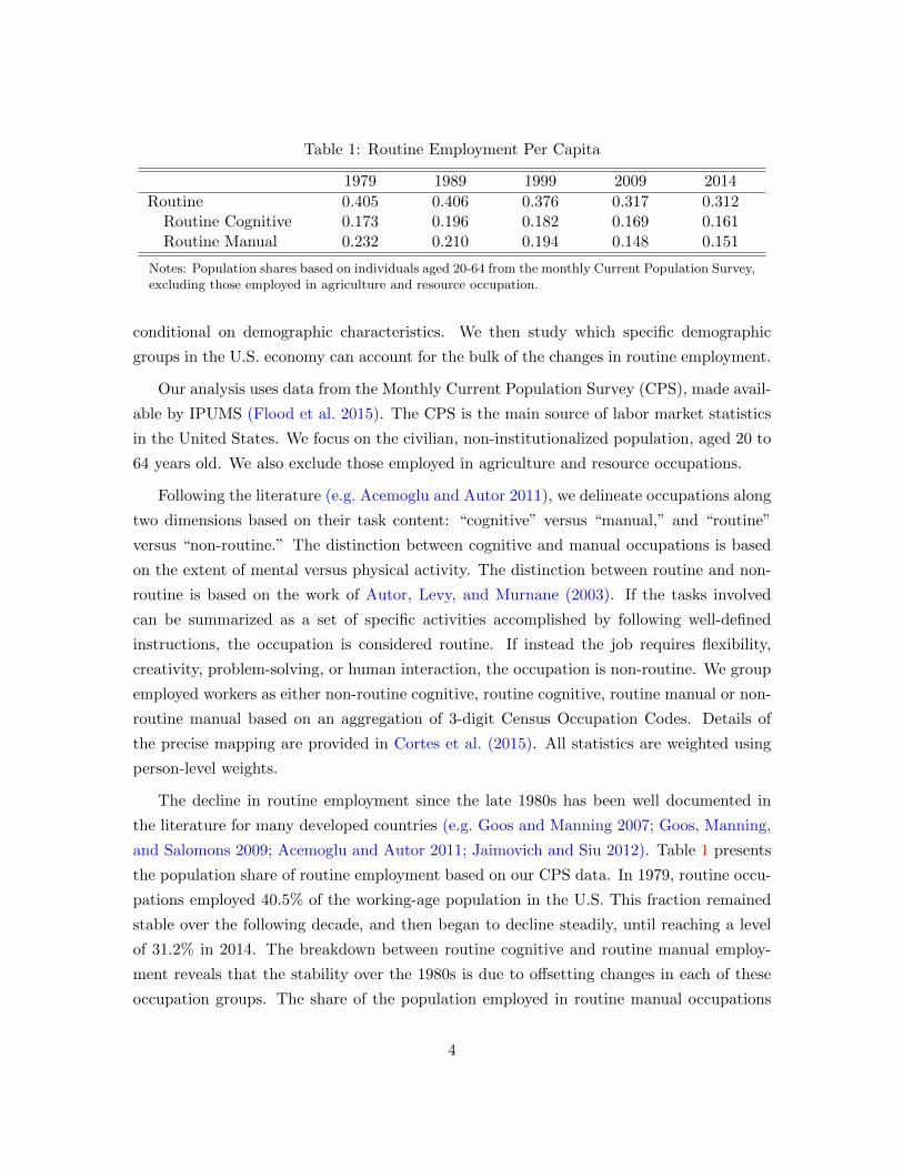
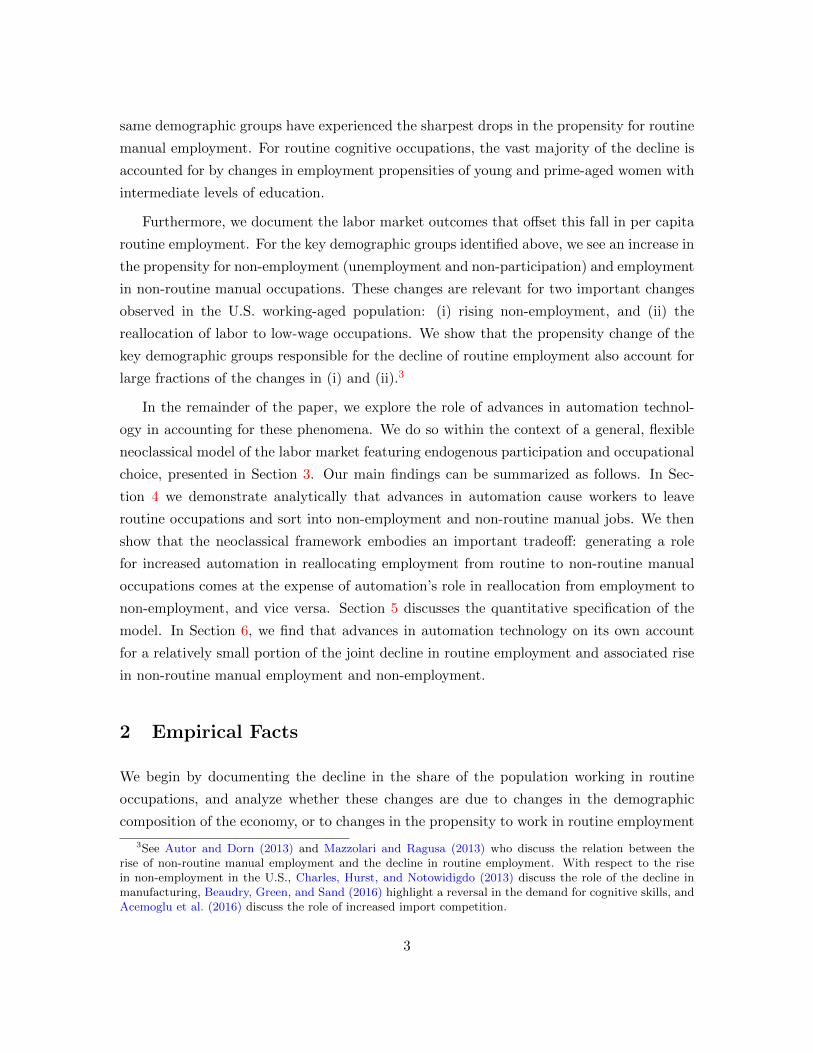
Table 1: Routine Employment Per Capita

1979 1989 1999 2009 2014

Routine 0.405 0.406 0.376 0.317 0.312Routine Cognitive 0.173 0.196 0.182 0.169 0.161Routine Manual 0.232 0.210 0.194 0.148 0.151

Notes: Population shares based on individuals aged 20-64 from the monthly Current Population Survey,excluding those employed in agriculture and resource occupation.

conditional on demographic characteristics. We then study which specific demographic

groups in the U.S. economy can account for the bulk of the changes in routine employment.

Our analysis uses data from the Monthly Current Population Survey (CPS), made avail-

able by IPUMS (Flood et al. 2015). The CPS is the main source of labor market statistics

in the United States. We focus on the civilian, non-institutionalized population, aged 20 to

64 years old. We also exclude those employed in agriculture and resource occupations.

Following the literature (e.g. Acemoglu and Autor 2011), we delineate occupations along

two dimensions based on their task content: “cognitive” versus “manual,” and “routine”

versus “non-routine.” The distinction between cognitive and manual occupations is based

on the extent of mental versus physical activity. The distinction between routine and non-

routine is based on the work of Autor, Levy, and Murnane (2003). If the tasks involved

can be summarized as a set of specific activities accomplished by following well-defined

instructions, the occupation is considered routine. If instead the job requires flexibility,

creativity, problem-solving, or human interaction, the occupation is non-routine. We group

employed workers as either non-routine cognitive, routine cognitive, routine manual or non-

routine manual based on an aggregation of 3-digit Census Occupation Codes. Details of

the precise mapping are provided in Cortes et al. (2015). All statistics are weighted using

person-level weights.

The decline in routine employment since the late 1980s has been well documented in

the literature for many developed countries (e.g. Goos and Manning 2007; Goos, Manning,

and Salomons 2009; Acemoglu and Autor 2011; Jaimovich and Siu 2012). Table 1 presents

the population share of routine employment based on our CPS data. In 1979, routine occu-

pations employed 40.5% of the working-age population in the U.S. This fraction remained

stable over the following decade, and then began to decline steadily, until reaching a level

of 31.2% in 2014. The breakdown between routine cognitive and routine manual employ-

ment reveals that the stability over the 1980s is due to offsetting changes in each of these

occupation groups. The share of the population employed in routine manual occupations

4

declines steadily over the entire 1979-2014 period. Meanwhile, the population share of rou-

tine cognitive employment increases between 1979 and 1989, and then declines steadily until

the end of our sample period. Given the different timing of the decline in routine manual

and routine cognitive employment, we separately analyze the 1979-2014 and the 1989-2014

periods.4

2.1 Decomposing Labor Market Changes

The past four decades have seen marked changes in the educational and age composition

of the economy. Since demographic groups differ in their propensity to work in routine

occupations, the decline of employment in these occupations may be partially accounted

for by these changes. On the other hand, routine employment may be declining because

of changes in the probability of working in such occupations for individuals with given

demographic characteristics. These changes would be indicative of economic forces that

change the labor market opportunities for specific groups of workers.

To investigate the relative importance of these two forces, we perform a set of decom-

positions where we divide the CPS sample into 24 demographic groups, based on:

• Age: 20-29 (hereafter, young), 30-49 (prime-aged), and 50+ years old (old);

• Education: less than high school completion, high school diploma, some post-secondary,

and college degree and higher;

• Gender: male and female.

Denoting the fraction of the population in labor market state j at time t as πjt , this can be

written as:

πjt =∑g

wgtπjgt, (1)

where wgt is the population share of demographic group g at time t, and πjgt is the fraction

of individuals of demographic group g in state j at t. We consider five labor market states:

employment in one of the four occupation groups described above, and non-employment

(unemployment and labor force non-participation).

4Jaimovich and Siu (2012) show that most of the decline in routine employment takes place duringrecessionary periods. In this paper we abstract from the exact timing of this decline and concentrate on thetotal change.

5

The change in the fraction of the population in labor market state j can be written as:

πj1 − πj0 =

∑g

wg1πjg1 −

∑g

wg0πjg0

=∑g

∆wg1πjg0 +

∑g

wg0∆πjg1 +∑g

∆wg1∆πjg1. (2)

The first term is a group size or composition effect, owing to the change in population

share of demographic groups over time. The second component is a propensity effect,

due to changes in the fraction of individuals within groups in state j. The third term is

an interaction effect capturing the co-movement of changes in group sizes and changes in

propensities.5

The results of this decomposition are presented in Table 2. We focus on two time

intervals: the 35 year period from 1979 to 2014 exhibiting a monotonic decline in per capita

employment in routine manual occupations in Panel A, and the period from 1989 to 2014

exhibiting a similar decline in routine cognitive employment in Panel B. Columns (1) and

(2) present the observed fraction of the population in each of the five labor market states

in the two time periods of interest. The total change in each of these population shares,

displayed in Column (3) is decomposed into the composition, propensity, and interaction

effect in Columns (4) through (6).

Panels A and B exhibit the well-documented increase in per capita employment in non-

routine cognitive (NRC) occupations. This can be accounted for by composition change in

the US population—the near doubling of the number of those with at least a college degree,

and to a lesser extent population aging (as both the highly educated and old have greater

propensities for NRC work). In addition, we see increases in non-routine manual (NRM)

employment in both periods, and a rise in non-employment between 1989 and 2014. Both

of these are accounted for by propensity change, which we discuss further in Section 2.4.

The changes of principal interest are the declines in per capita routine manual (RM)

employment in Panel A, and in per capita routine cognitive (RC) employment in Panel

B. First, with respect to the decline of RC we note that it is due entirely to declining

propensities. In fact, the changes in propensities account for more than 100% of the change

5We note that the common empirical approach to such accounting exercises is to perform a Oaxaca-Blinder (OB) decomposition (Oaxaca 1973; Blinder 1973). This would derive from a linear probabilityregression of inclusion in labor market states in which age, education, and gender effects would be assumedto be additively separable. Our approach in equation (2) is equivalent to a OB specification where theregressors include a full set of interactions between demographic characteristics. This allows us to accountfor heterogeneity between groups in terms of propensity changes. Nonetheless, we display the results of thestandard OB decomposition in Appendix A, and note that none of our findings are substantively altered.

6

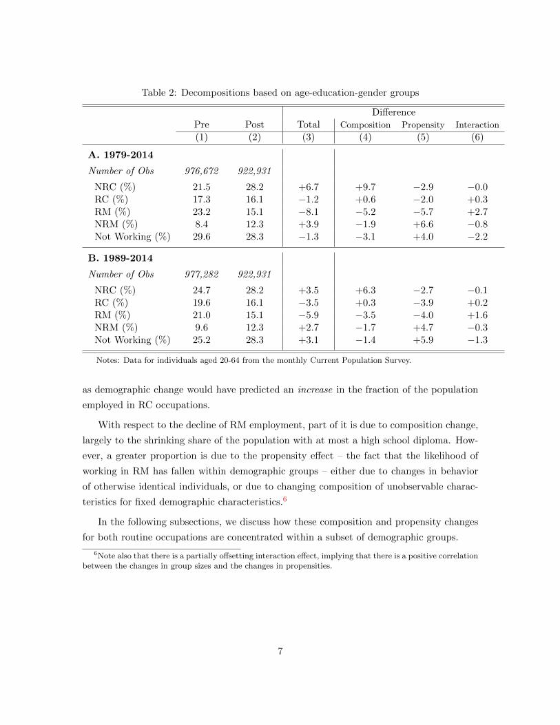
Table 2: Decompositions based on age-education-gender groups

DifferencePre Post Total Composition Propensity Interaction

(1) (2) (3) (4) (5) (6)

A. 1979-2014

Number of Obs 976,672 922,931

NRC (%) 21.5 28.2 +6.7 +9.7 −2.9 −0.0RC (%) 17.3 16.1 −1.2 +0.6 −2.0 +0.3RM (%) 23.2 15.1 −8.1 −5.2 −5.7 +2.7NRM (%) 8.4 12.3 +3.9 −1.9 +6.6 −0.8Not Working (%) 29.6 28.3 −1.3 −3.1 +4.0 −2.2

B. 1989-2014

Number of Obs 977,282 922,931

NRC (%) 24.7 28.2 +3.5 +6.3 −2.7 −0.1RC (%) 19.6 16.1 −3.5 +0.3 −3.9 +0.2RM (%) 21.0 15.1 −5.9 −3.5 −4.0 +1.6NRM (%) 9.6 12.3 +2.7 −1.7 +4.7 −0.3Not Working (%) 25.2 28.3 +3.1 −1.4 +5.9 −1.3

Notes: Data for individuals aged 20-64 from the monthly Current Population Survey.

as demographic change would have predicted an increase in the fraction of the population

employed in RC occupations.

With respect to the decline of RM employment, part of it is due to composition change,

largely to the shrinking share of the population with at most a high school diploma. How-

ever, a greater proportion is due to the propensity effect – the fact that the likelihood of

working in RM has fallen within demographic groups – either due to changes in behavior

of otherwise identical individuals, or due to changing composition of unobservable charac-

teristics for fixed demographic characteristics.6

In the following subsections, we discuss how these composition and propensity changes

for both routine occupations are concentrated within a subset of demographic groups.

6Note also that there is a partially offsetting interaction effect, implying that there is a positive correlationbetween the changes in group sizes and the changes in propensities.

7

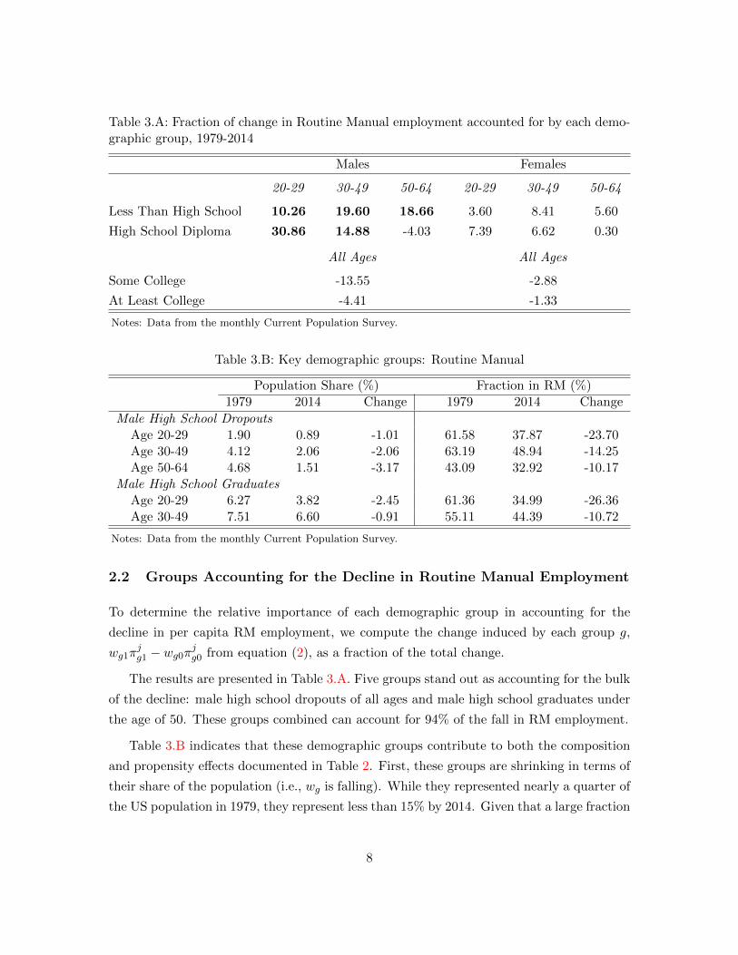
Table 3.A: Fraction of change in Routine Manual employment accounted for by each demo-graphic group, 1979-2014

Males Females

20-29 30-49 50-64 20-29 30-49 50-64

Less Than High School 10.26 19.60 18.66 3.60 8.41 5.60

High School Diploma 30.86 14.88 -4.03 7.39 6.62 0.30

All Ages All Ages

Some College -13.55 -2.88

At Least College -4.41 -1.33

Notes: Data from the monthly Current Population Survey.

Table 3.B: Key demographic groups: Routine Manual

Population Share (%) Fraction in RM (%)1979 2014 Change 1979 2014 Change

Male High School DropoutsAge 20-29 1.90 0.89 -1.01 61.58 37.87 -23.70Age 30-49 4.12 2.06 -2.06 63.19 48.94 -14.25Age 50-64 4.68 1.51 -3.17 43.09 32.92 -10.17

Male High School GraduatesAge 20-29 6.27 3.82 -2.45 61.36 34.99 -26.36Age 30-49 7.51 6.60 -0.91 55.11 44.39 -10.72


2.2 Groups Accounting for the Decline in Routine Manual Employment

To determine the relative importance of each demographic group in accounting for the

decline in per capita RM employment, we compute the change induced by each group g,

wg1πjg1 − wg0π

jg0 from equation (2), as a fraction of the total change.

The results are presented in Table 3.A. Five groups stand out as accounting for the bulk

of the decline: male high school dropouts of all ages and male high school graduates under

the age of 50. These groups combined can account for 94% of the fall in RM employment.

Table 3.B indicates that these demographic groups contribute to both the composition

and propensity effects documented in Table 2. First, these groups are shrinking in terms of

their share of the population (i.e., wg is falling). While they represented nearly a quarter of

the US population in 1979, they represent less than 15% by 2014. Given that a large fraction

8

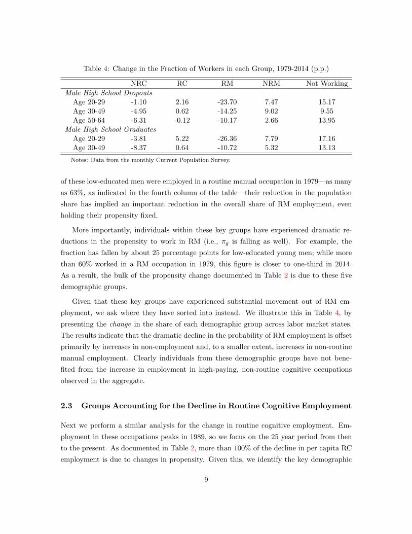
Table 4: Change in the Fraction of Workers in each Group, 1979-2014 (p.p.)

NRC RC RM NRM Not Working

Male High School DropoutsAge 20-29 -1.10 2.16 -23.70 7.47 15.17Age 30-49 -4.95 0.62 -14.25 9.02 9.55Age 50-64 -6.31 -0.12 -10.17 2.66 13.95

Male High School GraduatesAge 20-29 -3.81 5.22 -26.36 7.79 17.16Age 30-49 -8.37 0.64 -10.72 5.32 13.13


of these low-educated men were employed in a routine manual occupation in 1979—as many

as 63%, as indicated in the fourth column of the table—their reduction in the population

share has implied an important reduction in the overall share of RM employment, even

holding their propensity fixed.

More importantly, individuals within these key groups have experienced dramatic re-

ductions in the propensity to work in RM (i.e., πg is falling as well). For example, the

fraction has fallen by about 25 percentage points for low-educated young men; while more

than 60% worked in a RM occupation in 1979, this figure is closer to one-third in 2014.

As a result, the bulk of the propensity change documented in Table 2 is due to these five

demographic groups.

Given that these key groups have experienced substantial movement out of RM em-

ployment, we ask where they have sorted into instead. We illustrate this in Table 4, by

presenting the change in the share of each demographic group across labor market states.

The results indicate that the dramatic decline in the probability of RM employment is offset

primarily by increases in non-employment and, to a smaller extent, increases in non-routine

manual employment. Clearly individuals from these demographic groups have not bene-

fited from the increase in employment in high-paying, non-routine cognitive occupations

observed in the aggregate.

2.3 Groups Accounting for the Decline in Routine Cognitive Employment

Next we perform a similar analysis for the change in routine cognitive employment. Em-

ployment in these occupations peaks in 1989, so we focus on the 25 year period from then

to the present. As documented in Table 2, more than 100% of the decline in per capita RC

employment is due to changes in propensity. Given this, we identify the key demographic

9

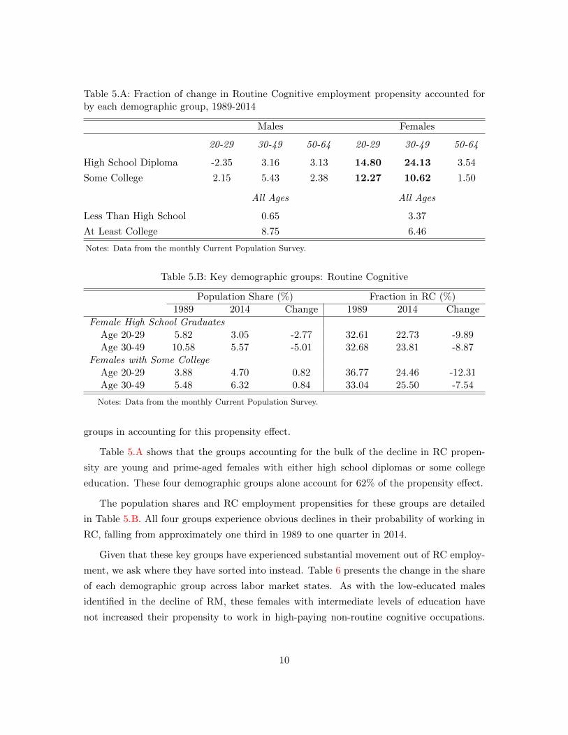
Table 5.A: Fraction of change in Routine Cognitive employment propensity accounted forby each demographic group, 1989-2014

Males Females

20-29 30-49 50-64 20-29 30-49 50-64

High School Diploma -2.35 3.16 3.13 14.80 24.13 3.54

Some College 2.15 5.43 2.38 12.27 10.62 1.50

All Ages All Ages

Less Than High School 0.65 3.37

At Least College 8.75 6.46


Table 5.B: Key demographic groups: Routine Cognitive

Population Share (%) Fraction in RC (%)1989 2014 Change 1989 2014 Change

Female High School GraduatesAge 20-29 5.82 3.05 -2.77 32.61 22.73 -9.89Age 30-49 10.58 5.57 -5.01 32.68 23.81 -8.87

Females with Some CollegeAge 20-29 3.88 4.70 0.82 36.77 24.46 -12.31Age 30-49 5.48 6.32 0.84 33.04 25.50 -7.54


groups in accounting for this propensity effect.

Table 5.A shows that the groups accounting for the bulk of the decline in RC propen-

sity are young and prime-aged females with either high school diplomas or some college

education. These four demographic groups alone account for 62% of the propensity effect.

The population shares and RC employment propensities for these groups are detailed

in Table 5.B. All four groups experience obvious declines in their probability of working in

RC, falling from approximately one third in 1989 to one quarter in 2014.

Given that these key groups have experienced substantial movement out of RC employ-

ment, we ask where they have sorted into instead. Table 6 presents the change in the share

of each demographic group across labor market states. As with the low-educated males

identified in the decline of RM, these females with intermediate levels of education have

not increased their propensity to work in high-paying non-routine cognitive occupations.

10

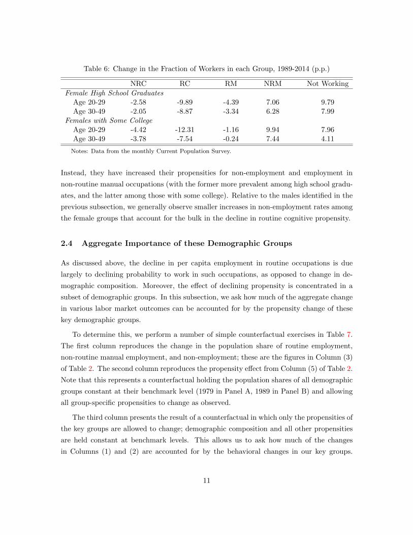
Table 6: Change in the Fraction of Workers in each Group, 1989-2014 (p.p.)

NRC RC RM NRM Not Working

Female High School GraduatesAge 20-29 -2.58 -9.89 -4.39 7.06 9.79Age 30-49 -2.05 -8.87 -3.34 6.28 7.99

Females with Some CollegeAge 20-29 -4.42 -12.31 -1.16 9.94 7.96Age 30-49 -3.78 -7.54 -0.24 7.44 4.11


Instead, they have increased their propensities for non-employment and employment in

non-routine manual occupations (with the former more prevalent among high school gradu-

ates, and the latter among those with some college). Relative to the males identified in the

previous subsection, we generally observe smaller increases in non-employment rates among

the female groups that account for the bulk in the decline in routine cognitive propensity.

2.4 Aggregate Importance of these Demographic Groups

As discussed above, the decline in per capita employment in routine occupations is due

largely to declining probability to work in such occupations, as opposed to change in de-

mographic composition. Moreover, the effect of declining propensity is concentrated in a

subset of demographic groups. In this subsection, we ask how much of the aggregate change

in various labor market outcomes can be accounted for by the propensity change of these

key demographic groups.

To determine this, we perform a number of simple counterfactual exercises in Table 7.

The first column reproduces the change in the population share of routine employment,

non-routine manual employment, and non-employment; these are the figures in Column (3)

of Table 2. The second column reproduces the propensity effect from Column (5) of Table 2.

Note that this represents a counterfactual holding the population shares of all demographic

groups constant at their benchmark level (1979 in Panel A, 1989 in Panel B) and allowing

all group-specific propensities to change as observed.

The third column presents the result of a counterfactual in which only the propensities of

the key groups are allowed to change; demographic composition and all other propensities

are held constant at benchmark levels. This allows us to ask how much of the changes

in Columns (1) and (2) are accounted for by the behavioral changes in our key groups.

11

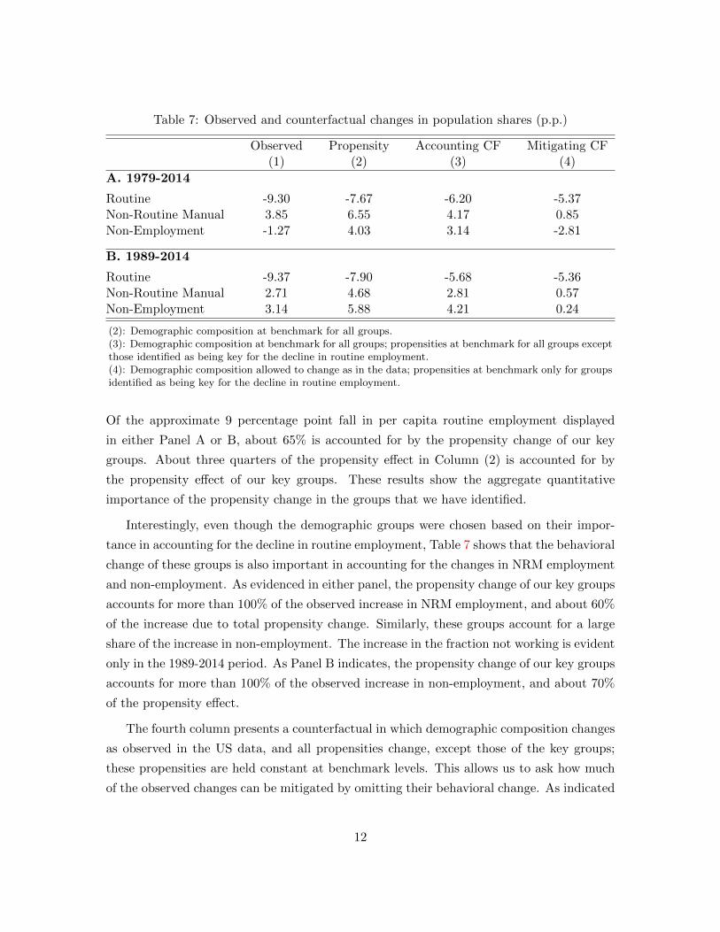
Table 7: Observed and counterfactual changes in population shares (p.p.)

Observed Propensity Accounting CF Mitigating CF(1) (2) (3) (4)

A. 1979-2014

Routine -9.30 -7.67 -6.20 -5.37Non-Routine Manual 3.85 6.55 4.17 0.85Non-Employment -1.27 4.03 3.14 -2.81

B. 1989-2014

Routine -9.37 -7.90 -5.68 -5.36Non-Routine Manual 2.71 4.68 2.81 0.57Non-Employment 3.14 5.88 4.21 0.24

(2): Demographic composition at benchmark for all groups.(3): Demographic composition at benchmark for all groups; propensities at benchmark for all groups exceptthose identified as being key for the decline in routine employment.(4): Demographic composition allowed to change as in the data; propensities at benchmark only for groupsidentified as being key for the decline in routine employment.

Of the approximate 9 percentage point fall in per capita routine employment displayed

in either Panel A or B, about 65% is accounted for by the propensity change of our key

groups. About three quarters of the propensity effect in Column (2) is accounted for by

the propensity effect of our key groups. These results show the aggregate quantitative

importance of the propensity change in the groups that we have identified.

Interestingly, even though the demographic groups were chosen based on their impor-

tance in accounting for the decline in routine employment, Table 7 shows that the behavioral

change of these groups is also important in accounting for the changes in NRM employment

and non-employment. As evidenced in either panel, the propensity change of our key groups

accounts for more than 100% of the observed increase in NRM employment, and about 60%

of the increase due to total propensity change. Similarly, these groups account for a large

share of the increase in non-employment. The increase in the fraction not working is evident

only in the 1989-2014 period. As Panel B indicates, the propensity change of our key groups

accounts for more than 100% of the observed increase in non-employment, and about 70%

of the propensity effect.

The fourth column presents a counterfactual in which demographic composition changes

as observed in the US data, and all propensities change, except those of the key groups;

these propensities are held constant at benchmark levels. This allows us to ask how much

of the observed changes can be mitigated by omitting their behavioral change. As indicated

12

in Panel A, if the propensity change of the key groups responsible for the decline of routine

employment had not occurred, NRM employment would only have risen by 0.85 percentage

points. This mitigates 3.00 ÷ 3.85 = 78% of the observed increase. Similarly, in Panel B,

omitting the key demographic groups mitigates (3.14− 0.24)÷ 3.14 = 92% of the observed

increase in non-employment.

To summarize, the changes in employment and occupational choice of a small subset of

demographic groups account for a large share of the decline in routine employment. These

same groups are also key in understanding the rise of non-employment observed in the past

25 years and, to a slightly lesser extent, the rise of non-routine manual employment observed

since 1979. This suggests that these long-run labor market changes may be closely linked

phenomena.

3 Model

Motivated by the findings of Section 2, we present a simple equilibrium model of the market

for those low- and middle-skill workers identified as most responsible for the decline in

routine employment over the past three decades. Our model is a generalized version of the

model analyzed in Autor and Dorn (2013), extended along two key dimensions. First, in

addition to making an occupational choice between routine and non-routine manual jobs,

individuals make a participation choice between working and non-employment.

Second, we conduct our analysis making only minimal functional form and distributional

assumptions on labor demand and labor supply. This generality allows us to characterize

the theoretical and quantitative implications of progress in automation technology on labor

market outcomes in a wide variety of parametric settings.

We use the model to study the role of advances in automation in rationalizing the

changes in sorting of workers across employment in routine occupations, non-routine man-

ual occupations, and non-employment. Given this goal, the analysis abstracts from other

changes observed in the U.S. economy. For example, changes in the share of high-skilled

workers and their occupational choice, changes in policy, and many other factors are likely

to have contributed to the labor market outcomes discussed in Section 2. By concentrating

solely on the impact of improvements in automation technology, we are able to present

precise results from a general framework, and provide a template for further quantitative

research in evaluating the role of automation.

13

3.1 Labor Demand

Our theoretical results can be derived from a very general specification of the demand for

labor. In particular, we assume that GDP, Yt, is produced with five factors of production

via:

Y = G(K,LC , LM ,

[A+ LER

]).

Here, K denotes capital (excluding the type of capital that relates to automation), LC

denotes the number of non-routine cognitive workers in the economy (“cognitive” hereafter),

LM denotes the number of non-routine manual workers (“manual”), LER denotes the effective

labor input of routine workers, and A denotes automation capital such as information and

communication technology capital (“ICT” hereafter). As we discuss below, the amount of

effective labor input differs from the measure of workers in the routine occupation. Effective

routine labor and automation capital are assumed to be perfect substitutes in the production

of “routine factor input” which we denote as R = A+LER. This assumption allows the model

to maximize the effect of automation on routine employment.

The representative firm hires factor inputs and sells output in competitive markets.

Profit maximization results in demand for routine and manual labor that equate wages to

marginal products:

WR = GR(K,LC , LM ,

[A+ LER

]), (3)

WM = GLM(K,LC , LM ,

[A+ LER

]). (4)

Note that WR denotes the wage per unit of effective labor.

3.2 Labor Supply

Since the key demographic groups identified in Section 2 work almost exclusively in routine

and manual occupations, we abstract from their ability to work in cognitive occupations.

Hence, low- and middle-skill workers choose between non-employment, working in “rou-

tine,” and working in “manual.” We assume that individuals make two discrete choices

sequentially: first a decision whether to participate in employment, and conditional on

deciding to work, an occupation decision.

Occupation Decision Individuals differ in their work ability, u, in the routine occupation

where u ∼ Γ (u), and Γ denotes the cumulative distribution function. Given the wage per

unit of effective labor, WR, a worker with ability u earns u×WR if employed in the routine

14

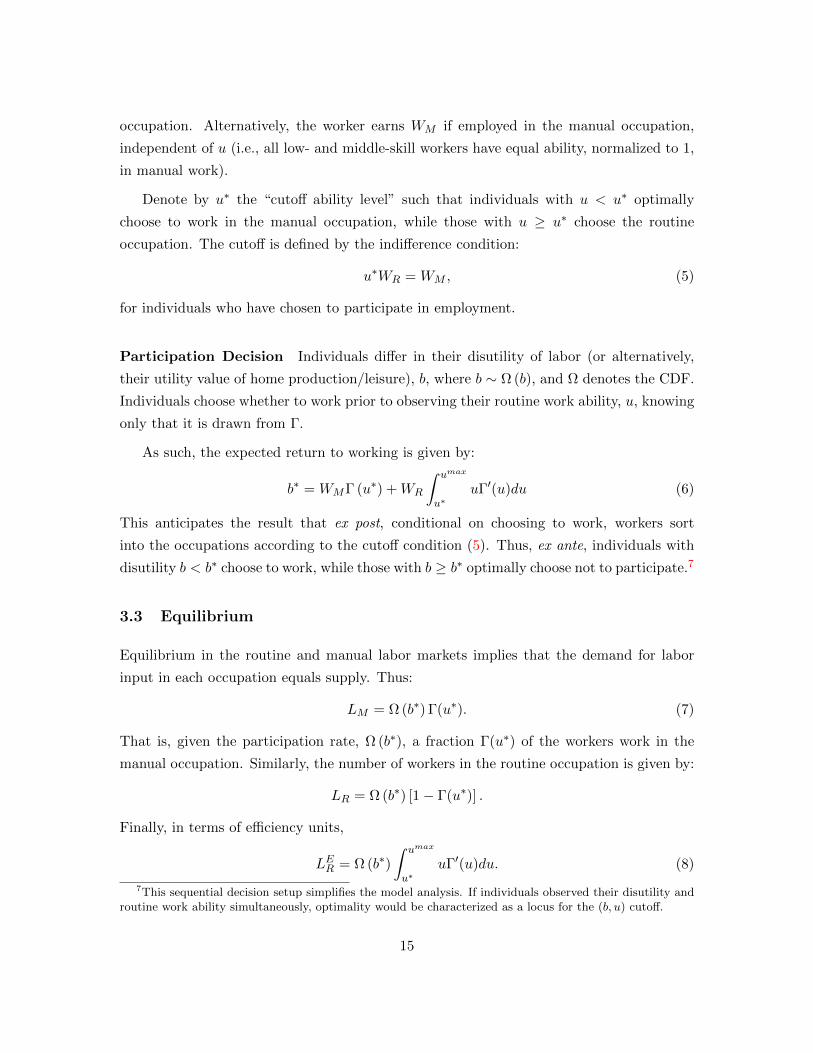
occupation. Alternatively, the worker earns WM if employed in the manual occupation,

independent of u (i.e., all low- and middle-skill workers have equal ability, normalized to 1,

in manual work).

Denote by u∗ the “cutoff ability level” such that individuals with u < u∗ optimally

choose to work in the manual occupation, while those with u ≥ u∗ choose the routine

occupation. The cutoff is defined by the indifference condition:

u∗WR = WM , (5)

for individuals who have chosen to participate in employment.

Participation Decision Individuals differ in their disutility of labor (or alternatively,

their utility value of home production/leisure), b, where b ∼ Ω (b), and Ω denotes the CDF.

Individuals choose whether to work prior to observing their routine work ability, u, knowing

only that it is drawn from Γ.

As such, the expected return to working is given by:

b∗ = WMΓ (u∗) +WR

∫ umax

u∗uΓ′(u)du (6)

This anticipates the result that ex post, conditional on choosing to work, workers sort

into the occupations according to the cutoff condition (5). Thus, ex ante, individuals with

disutility b < b∗ choose to work, while those with b ≥ b∗ optimally choose not to participate.7

3.3 Equilibrium

Equilibrium in the routine and manual labor markets implies that the demand for labor

input in each occupation equals supply. Thus:

LM = Ω (b∗) Γ(u∗). (7)

That is, given the participation rate, Ω (b∗), a fraction Γ(u∗) of the workers work in the

manual occupation. Similarly, the number of workers in the routine occupation is given by:

LR = Ω (b∗) [1− Γ(u∗)] .

Finally, in terms of efficiency units,

LER = Ω (b∗)

∫ umax

u∗uΓ′(u)du. (8)

7This sequential decision setup simplifies the model analysis. If individuals observed their disutility androutine work ability simultaneously, optimality would be characterized as a locus for the (b, u) cutoff.

15

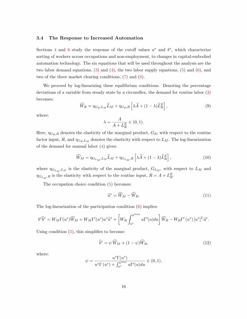
3.4 The Response to Increased Automation

Sections 4 and 6 study the response of the cutoff values u∗ and b∗, which characterize

sorting of workers across occupations and non-employment, to changes in capital-embodied

automation technology. The six equations that will be used throughout the analysis are the

two labor demand equations, (3) and (4), the two labor supply equations, (5) and (6), and

two of the three market clearing conditions, (7) and (8).

We proceed by log-linearizing these equilibrium conditions. Denoting the percentage

deviations of a variable from steady state by a circumflex, the demand for routine labor (3)

becomes:

WR = ηGR,LM LM + ηGR,R

[λA+ (1− λ)LER

], (9)

where:

λ =A

A+ LER∈ (0, 1).

Here, ηGR,R denotes the elasticity of the marginal product, GR, with respect to the routine

factor input, R, and ηGR,LM denotes the elasticity with respect to LM . The log-linearization

of the demand for manual labor (4) gives:

WM = ηGLM ,LM LM + ηGLM ,R

[λA+ (1− λ)LER

], (10)

where ηGLM ,LM is the elasticity of the marginal product, GLM , with respect to LM and

ηGLM ,R is the elasticity with respect to the routine input, R = A+ LER.

The occupation choice condition (5) becomes:

u∗ = WM − WR. (11)

The log-linearization of the participation condition (6) implies:

b∗b∗ = WMΓ(u∗)WM +WMΓ′(u∗)u∗u∗ +

[WR

∫ umax

u∗uΓ′(u)du

]WR −WRΓ′ (u∗) [u∗]2 u∗.

Using condition (5), this simplifies to become:

b∗ = ψ WM + (1− ψ)WR, (12)

where:

ψ =u∗Γ(u∗)

u∗Γ (u∗) +∫ umaxu∗ uΓ′(u)du

∈ (0, 1).

16

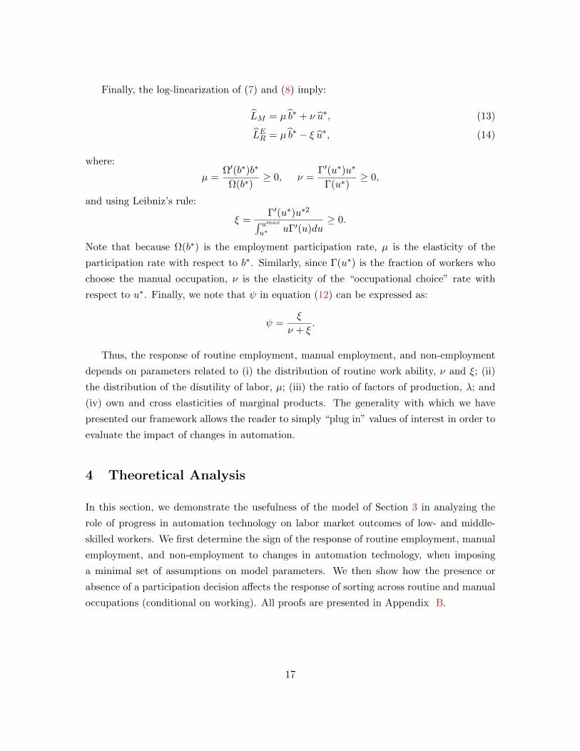
Finally, the log-linearization of (7) and (8) imply:

LM = µ b∗ + ν u∗, (13)

LER = µ b∗ − ξ u∗, (14)

where:

µ =Ω′(b∗)b∗

Ω(b∗)≥ 0, ν =

Γ′(u∗)u∗

Γ(u∗)≥ 0,

and using Leibniz’s rule:

ξ =Γ′(u∗)u∗2∫ umax

u∗ uΓ′(u)du≥ 0.

Note that because Ω(b∗) is the employment participation rate, µ is the elasticity of the

participation rate with respect to b∗. Similarly, since Γ(u∗) is the fraction of workers who

choose the manual occupation, ν is the elasticity of the “occupational choice” rate with

respect to u∗. Finally, we note that ψ in equation (12) can be expressed as:

ψ =ξ

ν + ξ.

Thus, the response of routine employment, manual employment, and non-employment

depends on parameters related to (i) the distribution of routine work ability, ν and ξ; (ii)

the distribution of the disutility of labor, µ; (iii) the ratio of factors of production, λ; and

(iv) own and cross elasticities of marginal products. The generality with which we have

presented our framework allows the reader to simply “plug in” values of interest in order to

evaluate the impact of changes in automation.

4 Theoretical Analysis

In this section, we demonstrate the usefulness of the model of Section 3 in analyzing the

role of progress in automation technology on labor market outcomes of low- and middle-

skilled workers. We first determine the sign of the response of routine employment, manual

employment, and non-employment to changes in automation technology, when imposing

a minimal set of assumptions on model parameters. We then show how the presence or

absence of a participation decision affects the response of sorting across routine and manual

occupations (conditional on working). All proofs are presented in Appendix B.

17

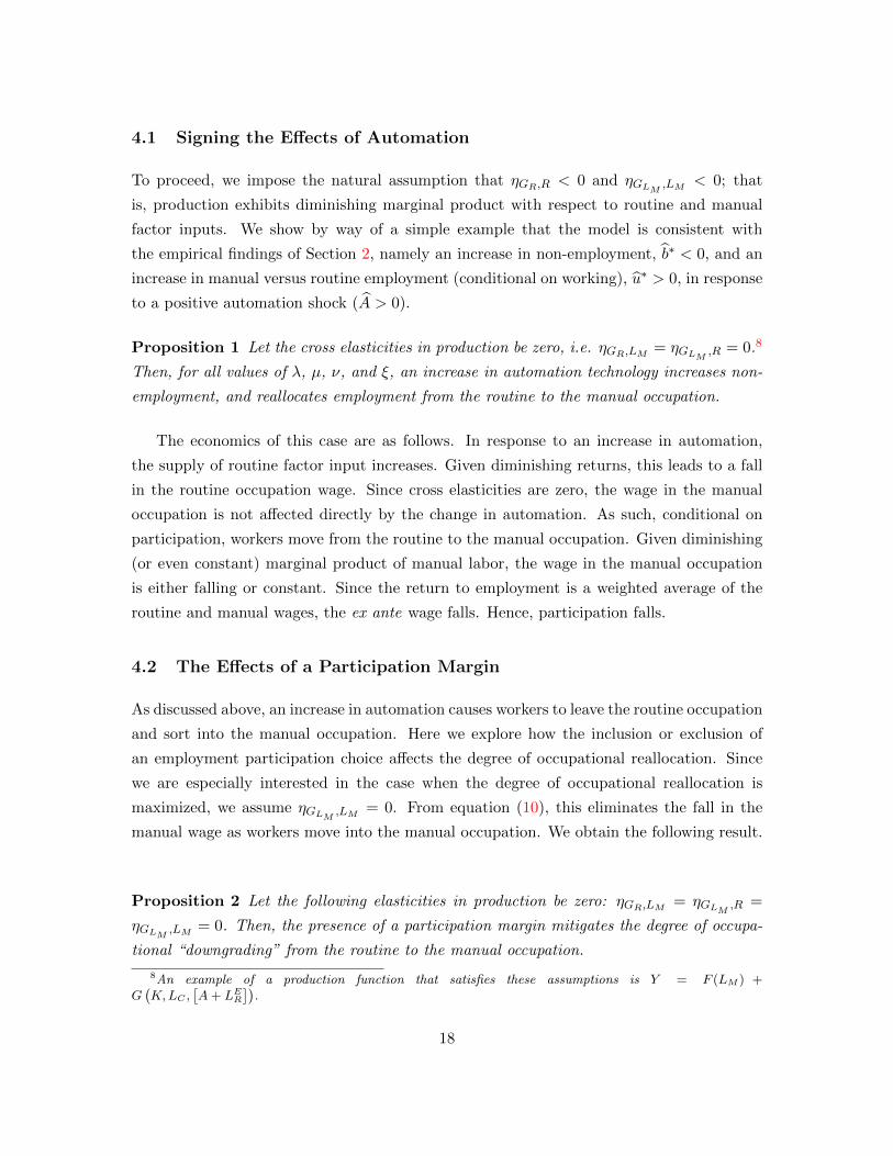
4.1 Signing the Effects of Automation

To proceed, we impose the natural assumption that ηGR,R < 0 and ηGLM ,LM < 0; that

is, production exhibits diminishing marginal product with respect to routine and manual

factor inputs. We show by way of a simple example that the model is consistent with

the empirical findings of Section 2, namely an increase in non-employment, b∗ < 0, and an

increase in manual versus routine employment (conditional on working), u∗ > 0, in response

to a positive automation shock (A > 0).

Proposition 1 Let the cross elasticities in production be zero, i.e. ηGR,LM = ηGLM ,R = 0.8

Then, for all values of λ, µ, ν, and ξ, an increase in automation technology increases non-

employment, and reallocates employment from the routine to the manual occupation.

The economics of this case are as follows. In response to an increase in automation,

the supply of routine factor input increases. Given diminishing returns, this leads to a fall

in the routine occupation wage. Since cross elasticities are zero, the wage in the manual

occupation is not affected directly by the change in automation. As such, conditional on

participation, workers move from the routine to the manual occupation. Given diminishing

(or even constant) marginal product of manual labor, the wage in the manual occupation

is either falling or constant. Since the return to employment is a weighted average of the

routine and manual wages, the ex ante wage falls. Hence, participation falls.

4.2 The Effects of a Participation Margin

As discussed above, an increase in automation causes workers to leave the routine occupation

and sort into the manual occupation. Here we explore how the inclusion or exclusion of

an employment participation choice affects the degree of occupational reallocation. Since

we are especially interested in the case when the degree of occupational reallocation is

maximized, we assume ηGLM ,LM = 0. From equation (10), this eliminates the fall in the

manual wage as workers move into the manual occupation. We obtain the following result.

Proposition 2 Let the following elasticities in production be zero: ηGR,LM = ηGLM ,R =

ηGLM ,LM = 0. Then, the presence of a participation margin mitigates the degree of occupa-

tional “downgrading” from the routine to the manual occupation.

8An example of a production function that satisfies these assumptions is Y = F (LM ) +G(K,LC ,

[A+ LER

]).

18

As we show in Appendix B, the response of the occupation cutoff to an automation

shock is given by:

u∗ =

[λ

(1− λ)ξ − 1ηGR,R

+ (1− ψ)(1− λ)µ

]A. (15)

Note that (1 − ψ)(1 − λ)µ ≥ 0, and recall from equations (13) and (14) that µ is

the elasticity of the participation rate with respect to b∗. Hence, everything else equal,

the response of occupational reallocation is maximized when participation does not adjust,

µ = 0. In other words, the higher is the elasticity parameter on participation, the smaller

is the movement of workers from routine to manual (conditional on working).

The intuition is as follows. An increase in automation technology drives down the

marginal product of routine labor. With a constant wage in the manual occupation, there

must be movement of labor out of the routine occupation, until the cutoff equation (5)

is satisfied for the marginal worker. When there is no employment participation choice,

the number of workers is fixed; all adjustment comes from occupational reallocation out

of routine jobs. With endogenous participation, some of the adjustment comes from fewer

workers selecting into employment. All else equal, a reduction in the number of workers

raises the marginal product of routine labor; this allows equilibrium to be attained with

less occupational reallocation than otherwise.

In summary, this proposition highlights an important tradeoff in neoclassical analyses

of automation’s impact on labor market outcomes. Maximizing the impact of advances

in automation on occupational reallocation requires abstracting from participation choice.

However, endogenizing the decision to work mitigates the impact on occupational sorting.

5 Quantitative Specification

In the next two sections we study the quantitative effect of automation. We first discuss the

quantitative specification of the model and present numerical results in Section 6. We pick

1989 as the “steady state” around which we linearize the model economy, since this year

corresponds to the maximum in per capita routine employment as displayed in Table 1.

5.1 Shares

Labor Values While the key demographic groups identified in Section 2 account for

the bulk of routine employment, other groups do account for important shares of manual

19

employment and non-employment. Appendix C details all the labor shares used in the

quantitative analysis, and we highlight selected values here that are relevant for our key

demographic groups.

Within the key groups, the employment rate was 72.7% in 1989, and conditional on

employment, the fraction working in routine occupations was 81.6%.9 Given a specification

of the distribution of routine work ability (discussed below), we calculate the average rou-

tine efficiency of our demographic groups. We use this average efficiency as the efficiency

of routine workers from all other demographic groups. This allows us to have a simple

aggregation of the effective routine labor input.

As a point of reference in evaluating the results of Section 6, the employment rate of

the key demographic groups fell to 64.9% by 2014, and the fraction of workers employed in

routine occupations fell to 69.1%.

Routine Factor Inputs Calibrating λ in equation (9) requires specifying the ratio of

service flows from automation capital, A, to effective routine labor, LER. Since we have

specified these inputs to be perfect substitutes in production, we can measure this ratio

empirically as the ratio of their factor shares of national income. Using CPS data and data

from Eden and Gaggl (2016) (see below) we obtain a 1989 value of λ = 0.0845.

5.2 Elasticities and Distributions

Participation Elasticity Recall that µ is the elasticity of the participation rate with

respect to b∗. To quantify this participation elasticity, we decompose the elasticity of the

participation rate with respect to b∗ into: (i) the elasticity of the participation rate with

respect to the wage, divided by (ii) the elasticity of b∗ with respect to the wage.

Part (i) can be identified empirically. The literature studying the earned income tax

credit (EITC) provides various estimates of the wage elasticity of the participation rate.

The handbook chapter by Hotz and Scholz (2003) suggests a value between 0.97 and 1.69.

As such we take 1.3 as a benchmark estimate. Part (ii) can be pinned down theoretically. In

particular, the cutoff condition, equation (12), implies that the elasticity of b∗ with respect

to an equal percentage change in the routine and manual wage equals 1. Hence, we specify

µ = 1.3 as a useful benchmark in our numerical analysis. However, given that the mapping

between the EITC literature and our model is not perfect, we consider also a higher value

9To align with the model, we exclude the 13.7% working in cognitive occupations.

20

of µ = 2.

Production Function Elasticities We restrict attention to the case when own elas-

ticities are negative, ηGR,R < 0 and ηGLM ,LM < 0. With respect to cross elasticities in

production, we consider several cases. First, we study the case where cross elasticities are

zero, i.e. ηGR,LM = ηGLM ,R = 0.

For the cases where the cross elasticities differ from zero we note that:

ηGR,LM ≡(∂GR∂LM

)(LMGR

)=

(∂GR∂LM

)(LMWR

),

ηGLM ,R ≡(∂GLM∂R

)(R

GLM

)=

(∂GLM∂R

)(R

WM

),

where the first and second condition are obtained from the fact that the firm’s FOCs (3)

and (4) require wages to equal marginal products. Using Young’s theorem, ∂GR/∂LM =

∂GLM /∂R, we have that:

ηGR,LMηGLM ,R

=WMLMWRR

=(WMLM )/Y

(WRR)/Y. (16)

Hence, the ratio of elasticities must equal the ratio of manual labor’s share of income to

the share of income paid to all routine factors of production.10 In the data, this ratio of

income shares is equal to 0.1355, disciplining the relative magnitude of cross elasticities. We

combine this with the fact that the product of the cross elasticities must equal the product

of the own elasticities:

ηGR,LM × ηGLM ,R ≡ ηGR,R × ηGLM ,LM . (17)

Together, (16) and (17) imply:

(WMLM )/Y

(WRR)/Y×(ηGLM ,R

)2= ηGR,R × ηGLM ,LM . (18)

This provides an empirical restriction on the (absolute value of the) cross elasticities as a

function of the own elasticities, while still permitting routine and manual inputs to be either

gross complements or substitutes. In considering different values of the own elasticities, we

refer to the empirical work of Lichter, Peichl, and Siegloch (2015) who conduct a meta

analysis of 151 different studies containing 1334 estimate of the own-wage elasticity of labor

demand. Specifically we consider the range of estimates that they provide for the U.S.

which lies between 0 and −3.11

10This uses the fact that the wage per unit of effective routine labor must equal the rental rate per unitof automation capital service flow in equilibrium.

11Lichter, Peichl, and Siegloch (2015) have assembled 287 estimates for the U.S. Of these, 11 are positive

21

Routine Ability Distribution Finally, to specify ν and ξ, we need to make choices

on the distribution of routine work ability, Γ. We consider three distinct cases. We first

consider a degenerate distribution of ability, equal to the ability in the manual occupation.

Assuming that workers are identical in both occupations allows us to generate sharp results

that are independent of the production elasticities. We discuss this in detail in Section 6.

In the remaining two cases, we assume the distribution to be either uniform or Pareto.

This allows us to explore the robustness of our findings regarding the impact of the automa-

tion shock. In the case of the uniform skill distribution, we have:

Γ(u) =u

umax,

where we normalize umin = 0. This implies:

ξ =umaxu∗2

umax − u∗, ν = 1.

In the case of the Pareto distribution:

Γ(u∗) = 1−(uminu∗

)κu.

This implies:

ξ = κu − 1, ν = κu

(uminu∗

)κu [1−

(uminu∗

)κu]−1.

Hence, in both cases, we have two values to pin down in order to specify ν and ξ. These

are umax and u∗ for the uniform, κu and (umin/u∗) for the Pareto. We use the same two

moments in the data to identify these. The first is the fraction of workers (conditional

on working) employed in the manual occupation in 1989, Γ(u∗) = 0.184. The second

data moment is the ratio of national income shares paid to routine and manual workers

in 1989; the ratio of income shares is given by(umax−u∗umaxu∗2

)for the uniform distribution and(

κuκu−1

) (uminu∗

)κu [1− (uminu∗

)κu]−1for the Pareto distribution. We measure this ratio to

equal 6.7568. Solving these two moment conditions for two unknowns results in ξ = 0.148

and ν = 1 for the uniform distribution, and ξ = 1.6798 and ν = 11.8664 for the Pareto

distribution.12

which we discard from the analysis. Of the remaining 276 estimates, about 95% lie between 0 and −3 whichis the range we consider. We are grateful to the authors of Lichter, Peichl, and Siegloch (2015) for kindlyshared their data with us; all errors in their use are our own.

12For the Uniform distribution ξ also equals the ratio of the manual to routine workers, hence the valueof 0.148 = 6.7568−1.

22

5.3 Automation Shock

To measure the magnitude of the “automation shock,” we relate capital-embodied automa-

tion technology to measured ICT capital using the data of Eden and Gaggl (2016). Simply

using the percentage growth rate of ICT capital between 1989 and 2014 neglects the fact

that along a balanced growth path (BGP) capital is expected to grow. As such, we measure

the shock as the deviation of ICT capital from a balanced growth trend.

To do so, we follow the approach of Greenwood, Herkowitz, and Krusell (1997). Specif-

ically, we assume that non-ICT capital evolves according to:

Kt+1 = (1− δK)Kt + INICT,t,

where δK denotes the depreciation rate and INICT,t denotes investment of non-ICT capital.

Similarly, ICT capital evolves according to:

At+1 = (1− δA)At + qt × IICT,t,

where δA and IICT denote the depreciation rate and investment, and q denotes ICT-specific

technological change. As in Greenwood, Herkowitz, and Krusell (1997), qt can be measured

as the inverse of the relative price of ICT to consumption goods at date t. With additivity

of the aggregate resource constraint (i.e. Y = IICT + INICT + C), the growth rate of ICT

capital along a BGP should have equalled the product of the economy’s growth rate and

the growth rate of q.

Eden and Gaggl (2016) construct the relative price and quantities of ICT capital and

estimate its depreciation rate.13 Taking these as exogenous, we construct the average growth

of q until 1989. Then, combining this with the growth rate of Real GDP starting in 1989,

we construct a counterfactual series for the stock of ICT capital that would have obtained

had the economy been along a BGP from 1989–2014. We then compare the actual to the

counterfactual series and find that the actual series is approximately 100 log points higher

in 2014. Thus, in our quantitative analysis we use A = 1 as our benchmark automation

shock and consider robustness to alternative values.

6 Numerical Results

In this section we evaluate the model’s quantitative predictions. Given an increase in capital-

embodied automation technology as measured in Section 5, we solve for the employment rate

13We are grateful to Eden and Gaggl for kindly shared their data with us; all errors are our own.

23

and occupational sorting between manual and routine occupations. Recall that in the data

between 1989–2014, for the key demographic groups, the employment rate fell from 72.7%

to 64.9%, and conditional on employment, the fraction working in manual occupations rose

from 18.4% to 30.9%.

We begin the analysis with the the case of a degenerate distribution of ability, equal to

the ability in the manual occupation. This serves as a useful benchmark. We then proceed

by considering heterogeneity in routine work ability.

6.1 Homogeneous Routine Ability

In this case all workers are equally productive in both occupations (with productivity nor-

malized to unity). Thus, in equilibrium WM = WR; furthermore, the participation equation

implies that b = WM = WR. In Appendix B we show that, irrespective of the production

elasticities, the response of the fraction of workers (conditional on working) who sort into

the manual occupation to an automation shock is given by:

(1− Γ(u∗))

(λ

1− λ

)A,

where, with a slight abuse of notation, (1 − Γ(u∗)) denotes the steady state fraction of

workers who sort into the routine occupation in 1989. Furthermore, the response of the

employment rate is given by:

− (1− Γ(u∗))

(λ

1− λ

)A.

This allows us to quantify the effects of automation easily. From Section 5, λ/(1−λ) =

0.0923. The fraction of workers in our demographic groups employed in manual occupations

was 0.184 in 1989. Given our estimate of A = 1, following the automation shock the fraction

of workers employed in manual occupations equals e[0.0923×(1−0.184)×1+log(0.184)] = 0.198.

Similarly, the employment rate falls to e[−0.0923×(1−0.184)×1+log(0.727)] = 0.6742. Recall that

the empirical values in 2014 are 30.9% for the fraction of workers employed in manual

occupations and 64.9% for the employment rate.

Finally, the simplicity of this analysis also allows us to ask what value of A is required to

“reverse engineer” the changes observed in the data. To account for all of the occupational

reallocation via the automation shock would require A = 6.04. This value would also allow

the model to explain more than 100% of the change in employment rate. Hence, the change

in automation technology, in log deviation terms, would need to be 6 times greater then

the one estimated in Section 5.

24

6.2 Heterogeneous Routine Ability

In this subsection, we analyze the case with heterogeneity in routine work ability when cross

elasticities in production are zero, i.e. ηGR,LM = ηGLM ,R = 0. This implies that changes

in automation do not have a direct effect on the marginal product of manual labor. We

find this case informative given the analytical results of Propositions 1 and 2 presented in

Section 4.

In the rest of this Section, we discuss the specification with Pareto distributed ability;

the results with the uniform distribution are presented in Appendix D. We solve the model

for various values of ηGR,R and ηGLM ,LM that lie in the interval [−3, 0), with the elasticity

of the participation rate initially set at the benchmark value of µ = 1.3. Recall that:

Ω (b∗) = Participation rate,

Γ(u∗) = Fraction in manual occupation,

implying that in the linearized equilibrium:

Ω′(b∗)b∗

Ω(b∗)b = µ× b = Participation rate,

Γ′(u∗)u∗

Γ(u∗)u = ν × u = Fraction in manual occupation.

For each combination of parameter values, the solution of the linearized model yields values

for u and b, from which we recover the level of participation and occupation sorting in

response to the automation shock.

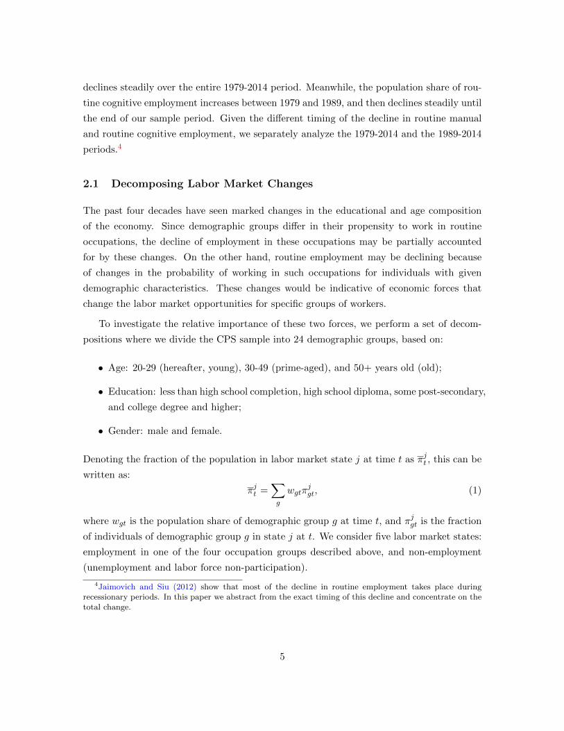
Each dot in Figure 1 depicts the employment rate (on the Y-axis) and, conditional on

working, the fraction of workers in manual occupations (on the X-axis) for specific pairs of

(ηGR,R, ηGLM ,LM ). These elasticities are reported, in that order, to the right of each dot

(for visual clarity we do so only for selected elasticity pairs).

Figure 1 illustrates that the effects of an increase in automation are of the correct

sign relative to Proposition 1: with the original, 1989 allocation located at the upper-left

corner, employment falls and workers reallocate toward the manual occupation. However,

matching either the observed change in the fraction of workers in manual occupation or the

employment rate is a challenge for the model. In terms of occupational reallocation, the

model can account for at most approximately 50%, represented by the point furthest to

the right in the diagram. In this parameterization, the model accounts for just less than

one third of the fall in the employment rate. This occurs when ηGLM ,LM = −0.001 and

25

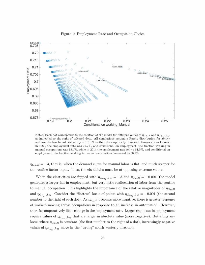
Figure 1: Employment Rate and Occupation Choice

Notes: Each dot corresponds to the solution of the model for different values of ηGR,R and ηGLM,LM

as indicated to the right of selected dots. All simulations assume a Pareto distribution for abilityand use the benchmark value of µ = 1.3. Note that the empirically observed changes are as follows:in 1989, the employment rate was 72.7%, and conditional on employment, the fraction working inmanual occupations was 18.4%, while in 2014 the employment rate fell to 64.9%, and conditional onemployment, the fraction working in manual occupations increased to 30.9%.

ηGR,R = −3, that is, when the demand curve for manual labor is flat, and much steeper for

the routine factor input. Thus, the elasticities must be at opposing extreme values.

When the elasticities are flipped with ηGLM ,LM = −3 and ηGR,R = −0.001, the model

generates a larger fall in employment, but very little reallocation of labor from the routine

to manual occupation. This highlights the importance of the relative magnitudes of ηGR,R

and ηGLM ,LM . Consider the “flattest” locus of points with ηGLM ,LM = −0.001 (the second

number to the right of each dot). As ηGR,R becomes more negative, there is greater response

of workers moving across occupations in response to an increase in automation. However,

there is comparatively little change in the employment rate. Larger responses in employment

require values of ηGLM ,LM that are larger in absolute value (more negative). But along any

locus where ηGR,R is constant (the first number to the right of a dot), increasingly negative

values of ηGLM ,LM move in the “wrong” south-westerly direction.

26

Hence, Figure 1 illustrates a quantitative tradeoff between responsiveness on the partic-

ipation and occupational sorting margins. Larger occupational reallocation requires smaller

values of ηGLM ,LM in absolute value (less negative), so that the manual wage does not fall

“too fast” in response to increased employment. But this relatively flat labor demand curve

implies little change in the employment rate. Generating larger responses of employment

to automation requires steep labor demand curves, resulting in relatively little response in

occupational sorting.

Figure 1 is also useful to explore the effect of heterogeneity on results. Near the bottom-

left corner of the figure, we plot the response generated from the version with homogenous

worker ability across occupations discussed above. For every point with ηGR,R < ηGLM ,LM

the amount of occupation reallocation is higher in the presence of heterogeneity. In fact,

this can be shown formally in the limiting case for ηGR,R < ηGLM ,LM = 0.14 The reason is as

follows. As workers move from routine to manual occupations, the routine wage rises. The

greater the heterogeneity in routine ability, the smaller is the impact of the marginal worker

on effective routine labor input which determines the wage (marginal product). Thus, with

greater heterogeneity, more reallocation of workers out of the routine occupation is required

to satisfy the occupational sorting condition, equation (11).

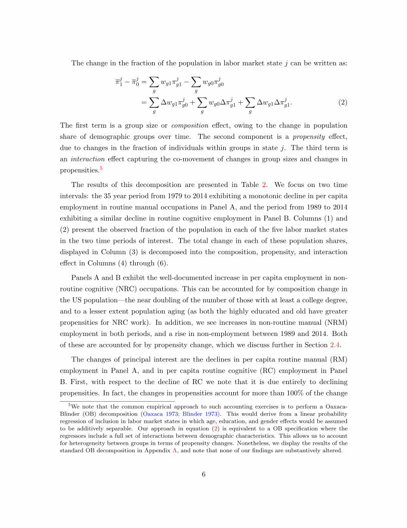
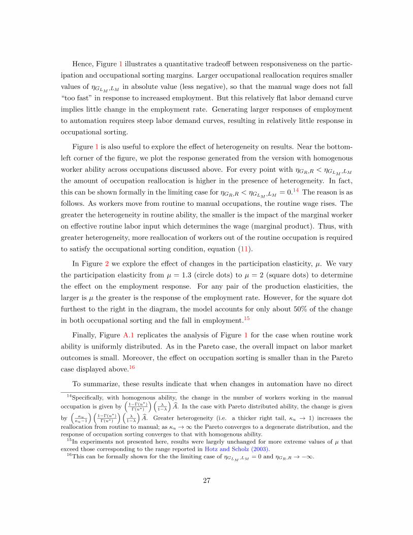
In Figure 2 we explore the effect of changes in the participation elasticity, µ. We vary

the participation elasticity from µ = 1.3 (circle dots) to µ = 2 (square dots) to determine

the effect on the employment response. For any pair of the production elasticities, the

larger is µ the greater is the response of the employment rate. However, for the square dot

furthest to the right in the diagram, the model accounts for only about 50% of the change

in both occupational sorting and the fall in employment.15

Finally, Figure A.1 replicates the analysis of Figure 1 for the case when routine work

ability is uniformly distributed. As in the Pareto case, the overall impact on labor market

outcomes is small. Moreover, the effect on occupation sorting is smaller than in the Pareto

case displayed above.16

To summarize, these results indicate that when changes in automation have no direct

14Specifically, with homogenous ability, the change in the number of workers working in the manual

occupation is given by(

1−Γ(u∗)Γ(u∗)

)(λ

1−λ

)A. In the case with Pareto distributed ability, the change is given

by(

κuκu−1

)(1−Γ(u∗)

Γ(u∗)

)(λ

1−λ

)A. Greater heterogeneity (i.e. a thicker right tail, κu → 1) increases the

reallocation from routine to manual; as κu →∞ the Pareto converges to a degenerate distribution, and theresponse of occupation sorting converges to that with homogenous ability.

15In experiments not presented here, results were largely unchanged for more extreme values of µ thatexceed those corresponding to the range reported in Hotz and Scholz (2003).

16This can be formally shown for the the limiting case of ηGLM,LM = 0 and ηGR,R → −∞.

27

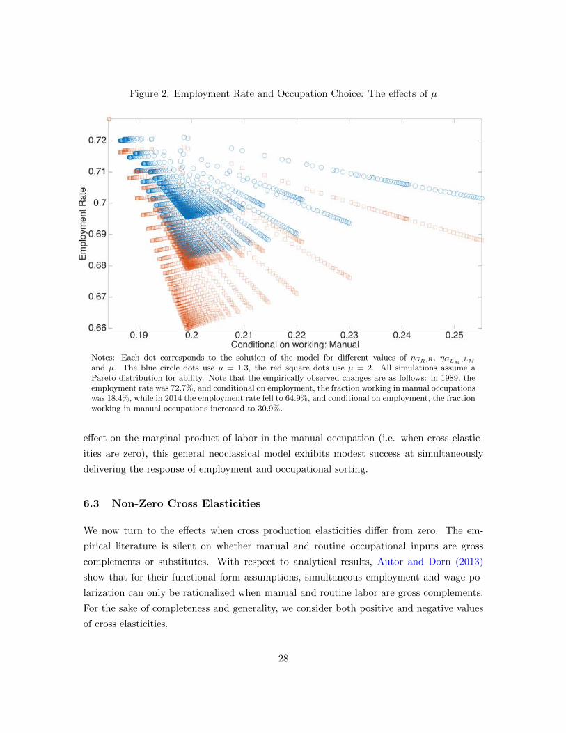
Figure 2: Employment Rate and Occupation Choice: The effects of µ

Notes: Each dot corresponds to the solution of the model for different values of ηGR,R, ηGLM,LM

and µ. The blue circle dots use µ = 1.3, the red square dots use µ = 2. All simulations assume aPareto distribution for ability. Note that the empirically observed changes are as follows: in 1989, theemployment rate was 72.7%, and conditional on employment, the fraction working in manual occupationswas 18.4%, while in 2014 the employment rate fell to 64.9%, and conditional on employment, the fractionworking in manual occupations increased to 30.9%.

effect on the marginal product of labor in the manual occupation (i.e. when cross elastic-

ities are zero), this general neoclassical model exhibits modest success at simultaneously

delivering the response of employment and occupational sorting.

6.3 Non-Zero Cross Elasticities

We now turn to the effects when cross production elasticities differ from zero. The em-

pirical literature is silent on whether manual and routine occupational inputs are gross

complements or substitutes. With respect to analytical results, Autor and Dorn (2013)

show that for their functional form assumptions, simultaneous employment and wage po-

larization can only be rationalized when manual and routine labor are gross complements.

For the sake of completeness and generality, we consider both positive and negative values

of cross elasticities.

28

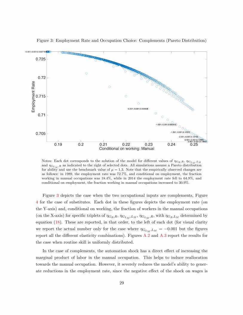
Figure 3: Employment Rate and Occupation Choice: Complements (Pareto Distribution)


and ηGLM,R as indicated to the right of selected dots. All simulations assume a Pareto distribution

for ability and use the benchmark value of µ = 1.3. Note that the empirically observed changes areas follows: in 1989, the employment rate was 72.7%, and conditional on employment, the fractionworking in manual occupations was 18.4%, while in 2014 the employment rate fell to 64.9%, andconditional on employment, the fraction working in manual occupations increased to 30.9%.

Figure 3 depicts the case when the two occupational inputs are complements, Figure

4 for the case of substitutes. Each dot in these figures depicts the employment rate (on

the Y-axis) and, conditional on working, the fraction of workers in the manual occupations

(on the X-axis) for specific triplets of ηGR,R, ηGLM ,LM , ηGLM ,R, with ηGR,LM determined by

equation (18). These are reported, in that order, to the left of each dot (for visual clarity

we report the actual number only for the case where ηGLM ,LM = −0.001 but the figures

report all the different elasticity combinations). Figures A.2 and A.3 report the results for

the case when routine skill is uniformly distributed.

In the case of complements, the automation shock has a direct effect of increasing the

marginal product of labor in the manual occupation. This helps to induce reallocation

towards the manual occupation. However, it severely reduces the model’s ability to gener-

ate reductions in the employment rate, since the negative effect of the shock on wages is

29

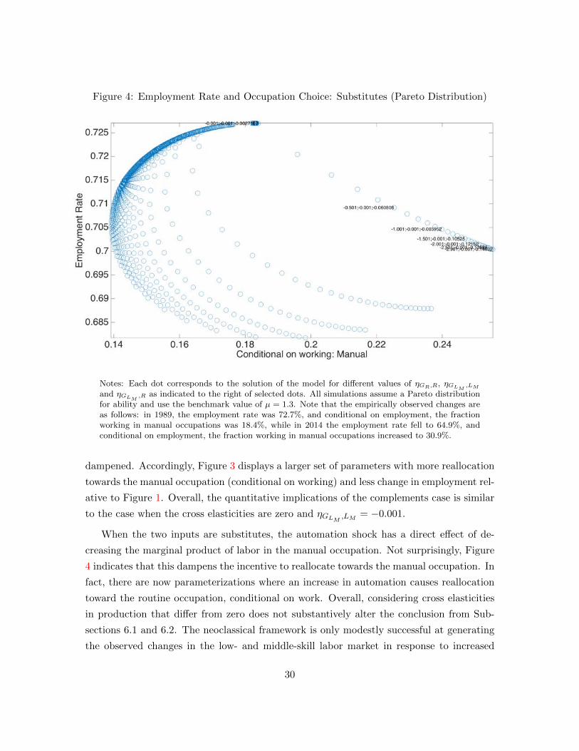
Figure 4: Employment Rate and Occupation Choice: Substitutes (Pareto Distribution)


and ηGLM,R as indicated to the right of selected dots. All simulations assume a Pareto distribution


dampened. Accordingly, Figure 3 displays a larger set of parameters with more reallocation

towards the manual occupation (conditional on working) and less change in employment rel-

ative to Figure 1. Overall, the quantitative implications of the complements case is similar

to the case when the cross elasticities are zero and ηGLM ,LM = −0.001.

When the two inputs are substitutes, the automation shock has a direct effect of de-

creasing the marginal product of labor in the manual occupation. Not surprisingly, Figure

4 indicates that this dampens the incentive to reallocate towards the manual occupation. In

fact, there are now parameterizations where an increase in automation causes reallocation

toward the routine occupation, conditional on work. Overall, considering cross elasticities

in production that differ from zero does not substantively alter the conclusion from Sub-

sections 6.1 and 6.2. The neoclassical framework is only modestly successful at generating

the observed changes in the low- and middle-skill labor market in response to increased

30

automation.17

6.4 What Would it Take?

Finally, we ask what the combination of parameter values and automation shock magnitude

is required to account for both the occupation reallocation and employment rate changes.

For the case of zero cross elasticity we find that doubling the log deviation shock (i.e. using

A = 2) comes close to matching the observed empirical changes. This is depicted in Figure

A.4 in the Appendix. This is similarly true for the case where the factors of production are

complements or substitutes, results we make available upon request.

It is important to note what these shock magnitudes mean. In our benchmark specifi-

cation, A = 1 in log terms, implying that ICT capital has nearly tripled (exp(1) = 2.71)

in levels relative to a balanced growth trend. A value of A = 2 implies a greater than

seven fold (exp(2) = 7.38) increase relative to a BGP. This highlights the challenge faced

by advances in automation, as represented by measured changes in ICT capital, as the

single force responsible for the changes in labor market outcomes experienced by the key

demographic groups studied here.

7 Conclusions

The share of employment in middle-skilled occupations has experienced a strong decline over

recent decades. In this paper we show that this is primarily due to a fall in the propensity

to work in these occupations conditional on demographic characteristics, rather than being

driven by changes in the demographic composition of the economy. Moreover, we show

that these propensity changes are concentrated among a relatively small subset of workers,

who have experienced an increase in their propensity for non-employment (unemployment

or non-participation) and their propensity to work in low-paying non-routine manual occu-

pations. In fact, we show that these groups can account for a substantial fraction of the

aggregate increase in non-employment and non-routine manual employment.

17We note that our findings contrast with those in vom Lehn (2015), and note two primary differences inthe analyses. In vom Lehn (2015), the skill distribution of the labor forces is allowed to change, generatingtime varying disutility from working. Here, we hold the distributions of labor disutilty and work abilityfixed and study only changes in automation. Finally, the nature of the experiments differ. We considerlabor market responses to deviations of the measured ICT capital stock from a BGP. By contrast, vom Lehn(2015) studies transition dynamics across steady states due to changes in the skill distribution and the timepath of equipment investment specific technical change, with stocks of equipment and structures determinedendogenously.

31

In order to shed light on the role of advances in automation technology in accounting

for these phenomena, we study a general, flexible neoclassical model of the labor market,

featuring endogenous occupational choice and participation decisions driven by worker het-

erogeneity. We demonstrate analytically that advances in automation cause workers to leave

routine occupations and sort into non-employment and non-routine manual jobs. However,

advances in automation technology on its own are unable to jointly generate changes in

occupational shares and employment propensities that are quantitatively similar to those

observed in the data for our demographic groups. We conclude that within the neoclassical

context, accounting for a significant fraction of the changes along both margins requires

relatively extreme combinations of parameter values and automation shock magnitude.

These results raise the question of what forces can account for our empirical findings.

The analysis in this paper has concentrated solely on the impact of automation. However,

other changes have occurred in the U.S. economy that could have affected occupational

choice and employment during the time period under study. Potentially relevant factors

that we have abstracted from include changes in the share of high-skilled workers and their

occupational choice, outsourcing and trade, and changes in policy affecting the incentive

to participation in the labor market. In our view, the generality of our model provides a

useful template for future quantitative research in evaluating the role of automation other

factors in contributing to the labor market outcomes discussed in the paper.

32

Appendix

A Oaxaca-Blinder Decomposition

In what follows, we further explore the labor market changes discussed in Subsection 2.1. To

do so, we perform a standard Oaxaca-Blinder (OB) decomposition analysis (Oaxaca 1973;

Blinder 1973) of population shares in each labor market state. Denoting πjit as a dummy

variable that takes on the value of 1 if individual i is in state j at time t and 0 otherwise,

we consider a simple linear probability model:

πjit = Xitβjt + εjit, (A.1)

Here, Xit denotes the demographic controls for age, education, and gender. The fraction in

labor market state j at time t is simply the sample average:

1

N

N∑i

πjit = πjt . (A.2)

The total change in the fraction between periods 1 and 0, πj1 − πj0, can be written as:

πj1 − πj0 = ∆Xi1β

j0 +Xi0∆βj1 + ∆Xi1∆βj1 (A.3)

Hence, this change can be decomposed into (i) a component that is explained by changes

in the demographic composition of the population over time, given the initial propensities βj0

(ii) a component unexplained by composition change, reflecting changes in the propensities

to work in occupation j for specific demographic groups, and (iii) a component that captures

the interaction between these two changes.

We perform this Oaxaca-Blinder decomposition separately for employment in each of

the four occupations, and for non-employment. The results are presented in Table A.1.

33

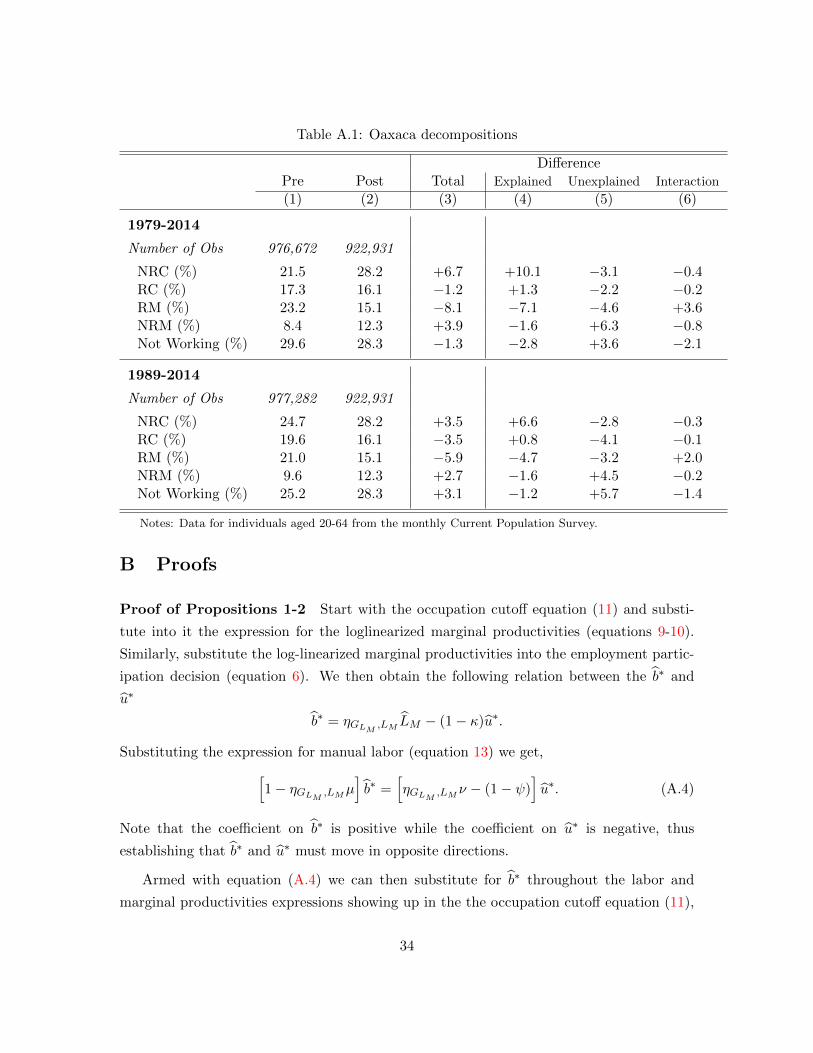
Table A.1: Oaxaca decompositions

DifferencePre Post Total Explained Unexplained Interaction

(1) (2) (3) (4) (5) (6)

1979-2014

Number of Obs 976,672 922,931

NRC (%) 21.5 28.2 +6.7 +10.1 −3.1 −0.4RC (%) 17.3 16.1 −1.2 +1.3 −2.2 −0.2RM (%) 23.2 15.1 −8.1 −7.1 −4.6 +3.6NRM (%) 8.4 12.3 +3.9 −1.6 +6.3 −0.8Not Working (%) 29.6 28.3 −1.3 −2.8 +3.6 −2.1

1989-2014

Number of Obs 977,282 922,931

NRC (%) 24.7 28.2 +3.5 +6.6 −2.8 −0.3RC (%) 19.6 16.1 −3.5 +0.8 −4.1 −0.1RM (%) 21.0 15.1 −5.9 −4.7 −3.2 +2.0NRM (%) 9.6 12.3 +2.7 −1.6 +4.5 −0.2Not Working (%) 25.2 28.3 +3.1 −1.2 +5.7 −1.4

Notes: Data for individuals aged 20-64 from the monthly Current Population Survey.

B Proofs

Proof of Propositions 1-2 Start with the occupation cutoff equation (11) and substi-

tute into it the expression for the loglinearized marginal productivities (equations 9-10).

Similarly, substitute the log-linearized marginal productivities into the employment partic-

ipation decision (equation 6). We then obtain the following relation between the b∗ and

u∗

b∗ = ηGLM ,LM LM − (1− κ)u∗.

Substituting the expression for manual labor (equation 13) we get,[1− ηGLM ,LMµ

]b∗ =

[ηGLM ,LM ν − (1− ψ)

]u∗. (A.4)

Note that the coefficient on b∗ is positive while the coefficient on u∗ is negative, thus

establishing that b∗ and u∗ must move in opposite directions.

Armed with equation (A.4) we can then substitute for b∗ throughout the labor and

marginal productivities expressions showing up in the the occupation cutoff equation (11),

34

ending up with the following equation that relates u∗ to the automation shock A,[ψ −

(ηGLM ,LM ν − (1− ψ)

1− ηGLM ,LMµ

)(1− ηGR,R(1− λ)µ)− ηGR,R(1− λ)ξ

]u∗ = −ηGR,RλA

(A.5)

Note that all of the coefficients multiplying on the left-hand-side u∗ are positive, and that

the coefficient in the right-hand-side multiplying A is positive as well. Thus, in response

to a positive automation shock the occupation cutoff increases. I.e. conditional on working

the share of workers who work in manual increases. Moreover, from equation (A.4) it then

follows that in response to a positive automation shock, employment rates fall.

Finally, we note that the proof of proposition 2 follows directly from equation (A.5).

Setting ηGLM = 0 and rearrange the terms then equation (15) follows. We note that

evaluating equation (15) with µ = 0 is indeed the result of a model where there is no

participation margin.

The Homogenous Agents Economy Abusing the notation of the heterogeneous agents

economy, denote the fraction of workers who are working by Ω and by Γ the fraction of

workers who conditional on working work in manual occupations. Thus, the measure of

manual and routine workers (from our key demographic groups) are given by

LM = ΩΓ

LR = Ω(1− Γ)

Log-linearizing these equations we obtain

LM = Ω + Γ

LR = Ω− Γ

1− ΓΓ

Since are indifferent between participating (which has a constant value) or working in

a manual or routine occupation it follows that

WR = WM = 0

Then, log-linearizing the marginal productivities expressions and substituting their values

into the cutoff condition above implies that LM = 0 and LR = − ALR

. LM = 0 implies then

that Ω = −Γ, and from LR = − ALRA and it follows that Γ = (1− Γ(u∗)) A

LRA.

35

Proof of Effects of Heterogeneity In the homogeneous agents economy all workers

are indifferent between working in manual and routine occupations. Hence WM = WR.

Substituting into this equation the expressions for the labor in routine and manual it then

follows that the change in the measure of workers working in manual occupation is given by(1−Γ(u∗)

Γ(u∗)

)ALRA. For the case of the heterogeneous economy, we follow the same strategy.

We start with the occupation cutoff equation (11) and substitute into it the expression for

the loglinearized marginal productivities (equations 9-10). This ends up with the following

relation between u∗ and A, u∗ = 1ξALERA. Then, to translate it into the measure of workers

working in manual occupation we need to multiply the right hand side by ν. Then, under

the Pareto distribution, νξ = κu

κu−1 .

C The Labor Expressions

While the key demographic groups identified in Section 2 account for the bulk of routine

employment, other groups do enter in and also account for important shares of manual

employment and non-employment and thus they matter for the calibration values in the

model (in terms of labor values and income shares). Below we list the values used in the

analysis; all are based on CPS data. All data refers to 1989 values which is the base for our

calibration.

The share of our demographic groups in the economy is 48.2%. 13.8% of our demographic

groups work in non-routine cognitive occupations which, to align with the model, we exclude

from our analysis. Then, since the employment rate of our demographic group is 72.7%

and, conditional on working 18.4% work in manual occupations, then in population our

key demographic groups contribute .482× .727× 0.184 into manual occupations. Since the

share in population of workers in manual occupations is 9.5% we allocated the remaining

4.01% to the “other demographic” groups. With the same approach, the contribution of our

demographic group to the routine share in population is given by .482× .727× (1− 0.184).

Since the share in population of workers in manual occupations is 40.5% we allocated the

remaining 15.90% to the “other demographic” groups.

Given a specification of the distribution of routine work ability (discussed in the main

body of the paper), we calculate the average routine efficiency of our demographic group.

We then use this average efficiency as the efficiency of routine workers from all other de-

mographic groups. This allows us to have a simple aggregation of the effective routine

labor input. For example for the Pareto distribution this average efficiency is given by

36

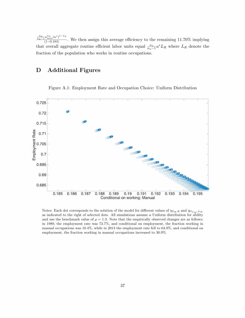
κuκu−1

uκumin(u∗)1−κu

(1−0.184) . We then assign this average efficiency to the remaining 11.70% implying

that overall aggregate routine efficient labor units equal κuκu−1u

∗LR where LR denote the

fraction of the population who works in routine occupations.

D Additional Figures

Figure A.1: Employment Rate and Occupation Choice: Uniform Distribution


as indicated to the right of selected dots. All simulations assume a Uniform distribution for abilityand use the benchmark value of µ = 1.3. Note that the empirically observed changes are as follows:in 1989, the employment rate was 72.7%, and conditional on employment, the fraction working inmanual occupations was 18.4%, while in 2014 the employment rate fell to 64.9%, and conditional onemployment, the fraction working in manual occupations increased to 30.9%.

37

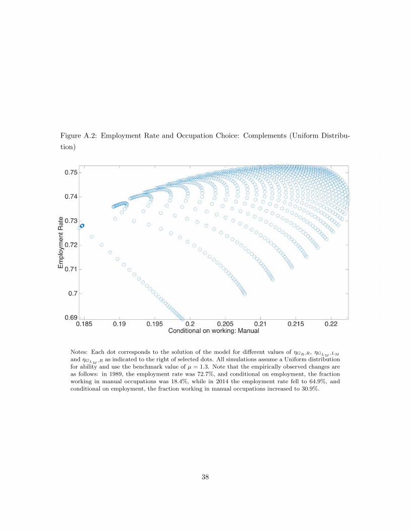
Figure A.2: Employment Rate and Occupation Choice: Complements (Uniform Distribu-

tion)


and ηGLM,R as indicated to the right of selected dots. All simulations assume a Uniform distribution


38

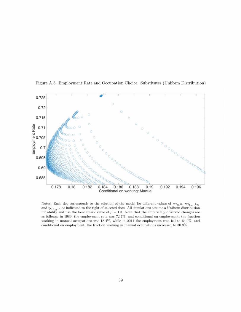
Figure A.3: Employment Rate and Occupation Choice: Substitutes (Uniform Distribution)


and ηGLM,R as indicated to the right of selected dots. All simulations assume a Uniform distribution


39

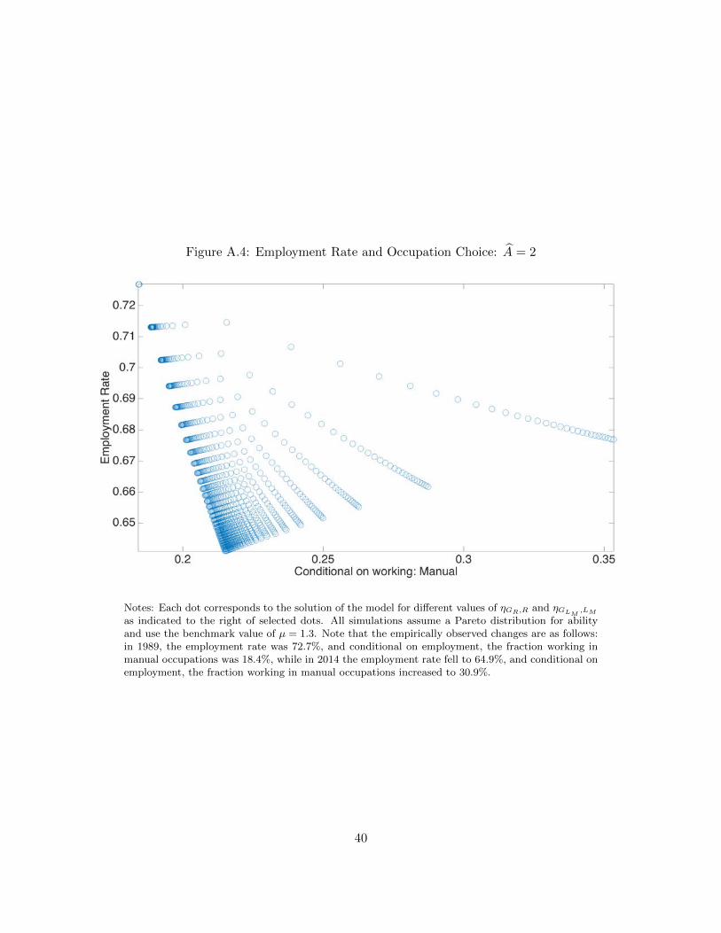
Figure A.4: Employment Rate and Occupation Choice: A = 2


as indicated to the right of selected dots. All simulations assume a Pareto distribution for abilityand use the benchmark value of µ = 1.3. Note that the empirically observed changes are as follows:in 1989, the employment rate was 72.7%, and conditional on employment, the fraction working inmanual occupations was 18.4%, while in 2014 the employment rate fell to 64.9%, and conditional onemployment, the fraction working in manual occupations increased to 30.9%.

40

References

Acemoglu, Daron and David Autor. 2011. “Skills, Tasks and Technologies: Implications for

Employment and Earnings.” In Handbook of Labor Economics, vol. 4B, edited by Orley

Ashenfelter and David Card, chap. 12. Elsevier, 1043–1171.

Acemoglu, Daron, David Autor, David Dorn, Gordon H. Hanson, and Brendan Price. 2016.

“Import Competition and the Great US Employment Sag of the 2000s.” Journal of Labor

Economics 34 (S1):S141 – S198.

Autor, David and David Dorn. 2009. “This Job Is “Getting Old”: Measuring Changes

in Job Opportunities Using Occupational Age Structure.” American Economic Review

99 (2):45–51.

Autor, David H. and David Dorn. 2013. “The growth of low skill service jobs and the

polarization of the U.S. labor market.” American Economic Review 103 (5):1553–1597.

Autor, David H., David Dorn, and Gordon H. Hanson. 2015. “Untangling trade and tech-

nology: Evidence from local labour markets.” The Economic Journal 125 (584):621–646.

Autor, David H., Frank Levy, and Richard J. Murnane. 2003. “The Skill Content Of Recent

Technological Change: An Empirical Exploration.” Quarterly Journal of Economics

118 (4):1279–1333.

Beaudry, Paul, David Green, and Benjamin Sand. 2016. “The Great Reversal in the Demand

for Skill and Cognitive Tasks.” Journal of Labor Economics 34 (S1):S199–S247.

Blinder, Alan. 1973. “Wage Discrimination: Reduced Form and Structural Estimates.”

Journal of Human Resources 8:436–455.

Charles, Kerwin Kofi, Erik Hurst, and Matthew J Notowidigdo. 2013. “Manufacturing

decline, housing booms, and non-employment.” NBER Working Paper No. 18949 .

Cortes, Guido Matias. 2016. “Where Have the Middle-Wage Workers Gone? A Study of

Polarization Using Panel Data.” Journal of Labor Economics 34 (1):63–105.

Cortes, Guido Matias, Nir Jaimovich, Christopher J. Nekarda, and Henry E. Siu. 2015.

“The Micro and Macro of Disappearing Routine Jobs: A Flows Approach.”

Eden, Maya and Paul Gaggl. 2016. “On the Welfare Implications of Automation.” Working

paper, University of North Carolina.

Flood, Sarah, Miriam King, Steven Ruggles, and J. Robert Warren. 2015. “Integrated

Public Use Microdata Series, Current Population Survey: Version 4.0. [Machine-readable

database].” Minneapolis: University of Minnesota .

41

Gaggl, Paul and Greg C. Wright. 2016. “A Short-Run View of What Computers Do:

Evidence from a UK Tax Incentive.” American Economic Journal: Applied Economics

Forthcoming.

Goos, Maarten and Alan Manning. 2007. “Lousy and Lovely Jobs: The Rising Polarization

of Work in Britain.” Review of Economics and Statistics 89 (1):118–133.

Goos, Maarten, Alan Manning, and Anna Salomons. 2009. “Job Polarization in Europe.”

American Economic Review: Papers & Proceedings 99 (2):58–63.

———. 2014. “Explaining Job Polarization: Routine-Biased Technological Change and

Offshoring.” American Economic Review 104 (8):2509–26.

Greenwood, Jeremy, Zvi Herkowitz, and Per Krusell. 1997. “The Own-Wage Elasticity of

Labor Demand: A Meta-Regression Analysis.” American Economic Review 87:342–362.

Gregory, Terry, Anna Salomons, and Ulrich Zierahn. 2016. “Racing With or Against the

Machine? Evidence from Europe.” ZEW - Centre for European Economic Research

Discussion Paper No. 16-053 .

Hotz, V. Joseph and John Karl Scholz. 2003. “The Earned Income Tax Credit.” In Means-

Tested Transfer Programs in the United States, edited by Robert A. Moffitt. University

of Chicago Press, 141–198.

Jaimovich, Nir and Henry E. Siu. 2012. “Job Polarization and Jobless Recoveries.” NBER

Working Paper 18334.

Lichter, Andreas, Andreas Peichl, and Sebastian Siegloch. 2015. “The Own-Wage Elasticity

of Labor Demand: A Meta-Regression Analysis.” European Economic Review 80:94–119.

Mazzolari, Francesca and Giuseppe Ragusa. 2013. “Spillovers from high-skill consumption

to low-skill labor markets.” Review of Economics and Statistics 95 (1):74–86.

Michaels, Guy, Ashwini Natraj, and John Van Reenen. 2014. “Has ICT polarized skill

demand? Evidence from eleven countries over twenty-five years.” Review of Economics

and Statistics 96 (1):60–77.

Morin, Miguel. 2016. “Computer Adoption and the Changing Labor Market.” Working

paper, Cambridge University.

Oaxaca, Ronald. 1973. “Male-Female Wage Differentials in Urban Labor Markets.” Inter-

national Economic Review 14:693–709.

vom Lehn, Christian. 2015. “Labor Market Polarization, the Decline of Routine Work,

and Technological Change: A Quantitative Analysis.” Working paper, Brigham Young

University.

42

Documents

DISAPPEARING ROUTINE JOBS: NATIONAL …workers towards non-employment. Quantitatively, we find that advances in automation technology on their own account for a relatively small portion