Embed Size (px)
Citation preview

Discipline of Engineering and Energy
Operation and Control Strategy of Coupled Microgrid
Clusters
S.M.Ferdous
This thesis is submitted in fulfilment of the requirements
for the Degree of
Doctor of Philosophy
at
Murdoch University
Perth, Australia
June 2021


i
Declaration
I declare that this thesis is my own account of my research and contains as its main
content work, which has not previously been submitted for a degree at any tertiary
education institution and all the relevant published works are duely cited.
S M Ferdous
S.M.Ferdous
June 2021

ii
Dedication
the philosophers and the mentors of my life
MY PARENTS

iii
Acknowledgement
I want to express my deepest gratitude to my principal supervisor Dr GM Shafiullah,
for his kind advice, invaluable guidance, encouragement, and support. I found him by
my side in every difficulty that I faced during PhD period. I have learned a lot from
his personality and knowledge. I am indebted to him for all those long discussions and
meetings, which played a significant role in my research. I am feeling very lucky to
have such wonderful, dynamic, and supportive supervisors.
I wish to express gratitude to my fellow colleagues at Murdoch University for all the
smiles, greetings, and tea-time chit-chats over the years. I would also like to thank my
colleagues- Dag, Mohammet, Remember, Jinping, and Kethaki for those social,
political and cultural discussions. I would also like to thank Zakir, Moktadir, Atiq,
Nipu, Zakia, Reza, Adnan, Ehsan and Amir for all the support and company. I wish to
express my special gratitude to Ishika, Iqbal, Hassan, Taskin, Shoeb, Pinky, Saif,
Shawon, Sohela, Kamrul and Vida. They have been the family here; without them, life
would be way too tricky.
I would also like to take this opportunity to express my gratefulness to my parents,
sister Tamanna and my newborn niece Mehrima for their belief, admiration, support,
and love.
Finally, all praise to almighty Allah, the Most merciful, and the controller of the
universe, without His mercy nothing would have been possible.
iv
Abstract
A standalone remote area microgrid may frequently experience overloading due to
lack of sufficient power generation or excessive renewable-based generation that can
cause unacceptable voltage and frequency deviation. This can lead the microgrid to
operate with less resiliency and reliability. Such problems are conventionally
alleviated by load-shedding or renewable curtailment. Alternatively, autonomously
operating microgrids in a geographical area can be provisionally connected to each
other to facilitate power exchange for addressing the problems of overloading or
overgeneration. The power exchange link among the microgrids can be of different
types such as a three-phase ac, a single-phase ac, or a dc-link. Power electronic
converters are required to interconnect such power exchange networks to the three-
phase ac microgrids and control the power-sharing amongst them. Such arrangement
is also essential to interconnect microgrid clusters to each other with proper isolation
while maintaining autonomy if they are operating in different standards. In this thesis,
the topologies, and structures of various forms of power exchange links are
investigated and appropriate operation and control frameworks are established under
which power exchange can take place properly. A decentralised control mechanism is
employed to facilitate power-sharing without any data communication. The dynamic
performance of the control mechanism for all the topologies is illustrated through
simulation studies in PSIM® while the stability and robustness of the operation are
evaluated using numerical studies in MATLAB®.
v
Table of Contents
Declaration ................................................................................................................... i
Dedication .................................................................................................................. ii
Acknowledgement ..................................................................................................... iii
Abstract ................................................................................................................. iv
Table of Contents ....................................................................................................... v
List of Figures ............................................................................................................ ix
List of Tables ............................................................................................................ xv
List of Abbreviations .............................................................................................. xvi
Chapter 1 Introduction ............................................................................................ 1
1.1. Background ................................................................................................ 1
1.2. Motivation .................................................................................................. 2
1.3. Research Objectives .................................................................................. 5
1.4. Outline of Research Contributions .......................................................... 5
1.5. Organisation of the Thesis ........................................................................ 6
Chapter 2 Literature review .................................................................................... 7
2.1. Operation of an Autonomous Microgrid ................................................. 7
2.2. Overloading and Excessive Generation in Microgrids .......................... 9
2.3. Coupling of Autonomous Microgrids .................................................... 10
2.4. Structure and Control of Coupled Microgrids ..................................... 11
2.5. Stability of Coupled Microgrids ............................................................. 13

vi
2.6. Topology Comparison for Coupled Microgrids .................................... 14
2.7. Summary ................................................................................................... 17
Chapter 3 Operational and Control Technique ................................................... 18
3.1 Microgrid Classification .......................................................................... 18
3.2 Various CMG structure and their control ............................................ 21
3.2.1 Three-phase AC interconnection (Topology-1) ..................................... 22
3.2.1.1 Control of MSC ........................................................................................ 22
3.2.1.1.1 Voltage Tracking and Switching Control .............................................. 23
3.2.1.1.2 Power Control .......................................................................................... 24
3.2.1.1.3 DC-link Voltage Control ......................................................................... 26
3.2.1.2 Control of LSC ......................................................................................... 27
3.2.1.2.1 LSC Control for HMG Operation .......................................................... 29
3.2.1.2.2 LSC Control for PMG Operation .......................................................... 32
3.2.2 Single-phase AC interconnection (Topology-2) .................................... 36
3.2.2.1 Control of MSC ........................................................................................ 36
3.2.2.2 Control of LSC ......................................................................................... 36
3.2.3 DC interconnection (Topology-3) ........................................................... 39
3.2.3.1 VSC Structure .......................................................................................... 40
3.2.3.2 VSC Control ............................................................................................. 40
3.2.3.2.1 VSC of an HMG ....................................................................................... 41
3.2.3.2.2 VSC of a PMG .......................................................................................... 41
3.3 Coordinated Power Sharing among BES and CMG ............................ 44
3.3.1 Network Structure ................................................................................... 44
3.3.2 Control of Converters .............................................................................. 45
3.3.2.1 Converters Structure ............................................................................... 46

vii
3.3.2.2 Converter Control Technique ................................................................ 46
3.3.3 Proposed Power Exchange Strategy ...................................................... 47
3.3.3.1 BES Control ............................................................................................. 49
3.3.3.2 Operation of BFC and BSC .................................................................... 51
3.3.3.3 Operation of IFC and ICC...................................................................... 53
3.4 Comparison among the three topologies ............................................... 55
3.5 Summary .................................................................................................. 57
Chapter 4 Time Domain Analysis ......................................................................... 58
4.1 Network Under Consideration ............................................................... 58
4.2 Performance Evaluation ......................................................................... 58
4.2.1 Topology-1 (Three-phase ac link) .......................................................... 59
4.2.1.1 Case Study-1 (Separate overloaded and over-generating PMG) ........ 59
4.2.1.2 Case Study-2 (Simultaneous overloaded and over-generating PMG) 63
4.2.2 Topology-2 ................................................................................................ 65
4.2.2.1 Case Study-1 (Overloaded PMG)........................................................... 65
4.2.2.2 Case Study-2 (Over-generating PMG) .................................................. 67
4.2.2.3 Case Study-3 (Two PMGs; one Overloaded and one Over-generating)
................................................................................................................... 69
4.2.3 Topology-3 ................................................................................................ 72
4.2.3.1 Case Study-1 (Balanced CMG) .............................................................. 72
4.2.3.2 Case Study-2 (Unbalanced CMG) .......................................................... 75
4.2.4 Coordinated Control Mechanism among BESs and CMGs ................ 77
4.2.4.1 Case Study-1 (Light Overloading) ......................................................... 79
4.2.4.2 Case Study-2 (Moderate Overloading) .................................................. 81
4.2.4.3 Case Study-3 (Controller Transition) .................................................... 83
viii
4.2.4.4 Case Study-4 (Heavy Overloading-1) ..................................................... 85
4.2.4.5 Case Study-5 (Heavy Overloading-2) ..................................................... 87
4.2.4.6 Case Study- 6 (Multiple MGs) ................................................................ 89
4.3 Comparison in performance of the three topologies ............................ 91
4.4 Summary ................................................................................................... 93
Chapter 5 Stability Analysis .................................................................................. 94
5.1. Stability Analysis ...................................................................................... 94
5.1.1. Variation of Droop Coefficients .............................................................. 94
5.1.2. Variation of PMG Power ........................................................................ 98
5.1.3. Variation of Line parameters ............................................................... 100
5.2. Summary ................................................................................................. 102
Chapter 6 Sensitivity Analysis ............................................................................. 103
6.1. Sensitivity Analysis ................................................................................ 103
6.1.1. Line Parameter Variation ..................................................................... 104
6.1.2. PMG Power Variation ........................................................................... 109
6.1.3. Number of MG variation in CMG ....................................................... 111
6.2. Summary ................................................................................................. 117
Chapter 7 Conclusions and recommendations .................................................. 118
7.1. Conclusions ............................................................................................. 118
7.2. Recommendations .................................................................................. 120
Appendix………………………………………………………………………… 121
References .............................................................................................................. 121
Publications Arising from this Thesis ................................................................... 134
ix
List of Figures
Figure 1.1 Microgrid interconnection through a common power exchange link. ....... 3
Figure 1.2 Topologies for Interlinking Converters used for power exchange links ... 3
Figure 2.1 Possible topologies for formation of coupled microgrid network ........... 12
Figure 3.1. Microgrid classification based on its frequency level. ........................... 19
Figure 3.2. Flowchart of the microgrid’s different mode of operation for power
exchange..................................................................................................................... 20
Figure 3.3. Assumed structure and close loop control mechanism of the MSC and LSC
for topology-1. ........................................................................................................... 21
Figure 3.4. Linear Quadratic Regulator based switching and voltage tracking. ....... 24
Figure 3.5. Block diagram of d and q axis current controller. .................................. 25
Figure 3.6. Block diagram of PQ controller for MSC. .............................................. 25
Figure 3.7. Block diagram of dc-link voltage controller for MSC ............................ 27
Figure 3.8. Frequency response plots of the control loops for the MSC. ................. 28
Figure 3.9. Modified angle-voltage droop control employed for the LSC during HMG
operation..................................................................................................................... 31
Figure 3.10. Frequency response plots of LSC operating under modified angle-voltage
droop control. ............................................................................................................. 31
x
Figure 3.11. Frequency controller of LSC for PMG operation in topology-1. ......... 33
Figure 3.12. Frequency controller for overload and over-generation prevention. .... 33
Figure 3.13. Assumed close loop control mechanism of frequency controller. ........ 33
Figure 3.14. Frequency response plots of LSC operating under frequency regulation
mode. .......................................................................................................................... 34
Figure 3.15. Block diagram of the PQ controller for LSC operation. ....................... 35
Figure 3.16. Assumed structure and close loop control mechanism of the MSC and
LSC for topology-2. ................................................................................................... 37
Figure 3.17. Linear Quadratic Regulator based switching and voltage tracking for
single-phase VSC. ...................................................................................................... 37
Figure 3.18. Frequency response of single-phase LSC operating under modified
angle-voltage droop control. ....................................................................................... 38
Figure 3.19. Block diagram of the PQ controller for single-phase LSC. .................. 38
Figure 3.20. VSC operation for topology-3 (a) VSC structure, (b) Closed-loop control
system. ........................................................................................................................ 40
Figure 3.21. Frequency regulation controller of VSC for PMG operation in
topology- 3. ................................................................................................................ 43
Figure 3.22. Autonomous CMG network with BES to coordinate power sharing .... 45
Figure 3.23. Assumed structure and closed-loop control block diagram of VSC and
filter system for BSC/ICC .......................................................................................... 46
Figure 3.24. Overall block diagram of the proposed coordinated power exchange
mechanism among BES and CMG network ............................................................... 48
xi
Figure 3.25. BES nominal operation scheme- (a) charging mode (b) discharging mode
.................................................................................................................................... 49
Figure 3.26. Different mode of operation of BES. .................................................... 50
Figure 3.27 Control of BES different operation modes ............................................ 50
Figure 3.28. Proposed overload management scheme and its different modes of
operation..................................................................................................................... 51
Figure 3.29. Control mechanism of BSC for overload management ........................ 52
Figure 3.30. Control mechanism of ICC for overload management ......................... 54
Figure 4.1 Simulation results of case study-1 for topology- 1. ................................. 61
Figure 4.2 Simulation results of case study-2 for topology- 1. ................................. 64
Figure 4.3 Simulation results of case study-1 for topology- 2. ................................. 66
Figure 4.4 Simulation results of case study-2 for topology- 2. ................................. 68
Figure 4.5 Simulation results of case study-3 for topology- 2. ................................. 70
Figure 4.6 Simulation results of case study-1 for topology- 3. ................................. 73
Figure 4.7 Simulation results of case study-2 for topology- 3. ................................. 76
Figure 4.8 Status of self-healing agents and converters in 6 different case studies. . 78
Figure 4.9 Simulation results for light overloading in case study-1. ........................ 80
Figure 4.10 Simulation results for moderate overloading in case study-2. ............... 82
Figure 4.11 Simulation results for controller transition in case study-3. .................. 84
Figure 4.12 Simulation results for heavy overloading- 1 in case study- 4. ............... 86
Figure 4.13 Simulation results for heavy overloading- 2 in case study- 5. ............... 88
xii
Figure 4.14 Simulation results for Multiple microgrids in case study- 6. ................. 90
Figure 5.1 CMG Stability analysis for topology-1: Eigenvalue trajectory for variation
of droop coefficients ................................................................................................... 95
Figure 5.2 CMG Stability analysis for topology-2: Eigenvalue trajectory for variation
of droop coefficients ................................................................................................... 95
Figure 5.3 CMG Stability analysis for topology-1: Eigenvalue trajectory for variation
of droop coefficients .................................................................................................. 96
Figure 5.4 CMG Stability analysis for topology-2: Eigenvalue trajectory for variation
of droop coefficients. .................................................................................................. 96
Figure 5.5 CMG Stability analysis for topology-3: Eigenvalue trajectory for variation
of droop coefficients ................................................................................................... 97
Figure 5.6 CMG Stability analysis for topology-1: Eigenvalue trajectory for PMG
Power variation ........................................................................................................... 99
Figure 5.7 CMG Stability analysis for topology-2: Eigenvalue trajectory for PMG
Power variation ........................................................................................................... 99
Figure 5.8 CMG Stability analysis for topology-3: Eigenvalue trajectory for PMG
Power variation ......................................................................................................... 100
Figure 5.9 CMG Stability analysis for topology-1: Eigenvalue trajectory for line
impedance variation. ................................................................................................ 100
Figure 5.10 CMG Stability analysis for topology-2: Eigenvalue trajectory for line
impedance variation. ................................................................................................ 101
Figure 5.11 CMG Stability analysis for topology-3: Eigenvalue trajectory for line
resistance variation. .................................................................................................. 101
xiii
Figure 6.1 Comparative CMG sensitivity analysis of topology-1 and 2 for line
impedance variation. ................................................................................................ 105
Figure 6.2 Effect of line impedance variation on CMG network for topology-1 ... 106
Figure 6.3 Effect of line impedance variation on CMG network for topology-2 ... 106
Figure 6.4 CMG sensitivity analysis of topology-3 for line resistance variation ... 108
Figure 6.5 Effect of line resistance variation on CMG network for topology-3. .... 109
Figure 6.6 Comparative CMG sensitivity analysis of topology-1 and 2 for PMG power
variation ................................................................................................................... 110
Figure 6.7 Sensitivity analysis of the CMG network in topology-3 with PMG power
demand variation. ..................................................................................................... 111
Figure 6.8 Stability margin comparison of the power control loop for topology-1 with
varying number of microgrids to form CMG........................................................... 112
Figure 6.9 Stability margin comparison of the power control loop for topology-1 with
varying number of microgrids to form CMG........................................................... 112
Figure 6.10 Stability margin comparison of the power control loop for topology-3 with
varying number of MGs to form CMG. ................................................................... 113
Figure 6.11 Stability margin comparison of the frequency control loop for topology-
1 with varying number of MGs to form CMG. ........................................................ 114
Figure 6.12 Stability margin comparison of the frequency control loop for topology-
2 with varying number of MGs to form CMG. ........................................................ 114
Figure 6.13 Stability margin comparison of the frequency control loop for topology-
3 with varying number of MGs to form CMG. ........................................................ 115

xiv
Figure 6.14 Stability margin comparison of the dc power exchange link for topology-
3 with varying number of MGs to form CMG. ........................................................ 116
xv
List of Tables
Table 2.1 Comparison of different CMG features. ................................................... 16
Table 3.1 Classification of microgrids based on their frequency .............................. 20
Table 3.2 Comparison of different topologies employed for power exchange link .. 56
Table 4.1 Technical data of network under consideration ........................................ 60
Table 4.2 Events applied to microgrids in Case-1 at different intervals ................... 62
Table 4.3 Overloading and over-generating events applied to microgrids in Case-2 at
different intervals ....................................................................................................... 65
Table 4.4 Events applied to microgrids in Case-1 at different intervals for overloading
scenario. ..................................................................................................................... 67
Table 4.5 Events applied to microgrids in Case-2 at different intervals for over-
generation scenario. ................................................................................................... 69
Table 4.6 Overloading and over-generating events applied to microgrids in Case-3 at
different intervals. ...................................................................................................... 71
Table 4.7 Events applied to microgrids in Case-1 at different intervals.. ................. 74
Table 4.8 Over-generation and overloading events applied to microgrids in Case-2 at
different intervals. ...................................................................................................... 77

xvi
List of Abbreviations
BES Battery Energy Storage
BFC Battery Frequency Controller
BSC Battery Storage Converter
CMG Coupled Microgrid
DER Distributed energy resource
DG Distributed Generator
FFT Fast Fourier Transform
FMG Floating Microgrid
HMG Healthy Microgrid
ICC Interconnection Converter
IFC Interconnection Frequency Controller
LPF Low Pass Filter
LQR Linear Quadratic Regulator
LSC Line-Side Converter
MG Microgrid
MSC Microgrid Side Converter
OG Over-generation
OGFC Over-generation Frequency Controller
OL Overload
OLFC Overload Frequency Controller
PMG Problem Microgrid
PCC Point of Common Coupling
PI Proportional-integral
PLL Phase-Locked Loop
VSC Voltage Source Converter

Chapter 1. Introduction
1
Chapter 1 Introduction
This chapter provides the background and motivation of the conducted research in this
thesis. The key research objectives and contributions of the thesis are highlighted and
summarised. Finally, the organisation of the thesis, concerning each following chapter,
has been introduced.
1.1. Background
A microgrid is usually referred to as a small-scale interconnected network of multiple
Distributed Generators (DG) that are predominantly renewable energy source-based
and power electronic converter-interfaced, distributed loads, and energy storage [1-3].
Such a system can operate under a centralised, semi-centralised, or decentralised
control scheme [2, 4-6], that may have two modes of grid-connected and autonomous
(islanded). Where a utility grid is not feasible or unavailable due to cost and economic
constraint, e.g., the edge-of-grid or remote/regional areas, the microgrids can operate
under a decentralised control scheme and permanently autonomous, to minimise the
cost by saving the requirement of communication technologies and thus facilitating to
integrate a large number of renewable sources [4-7]. One or some DGs in such a
scheme usually operates based on droop control to realise the desired power-sharing
amongst them while also regulating the desired frequency and voltage [8-13]. Thus,
the active and reactive powers are regulated at the output of each DG operating in
droop control, and the microgrid’s voltage and frequency are regulated within the
acceptable limits and thus, the system’s stability will be maintained [14-18].
To electrifying remote and regional areas, autonomous microgrids are a cost-effective
solution and preferred over commissioning long transmission and distribution lines.
Hence, microgrids operating permanently in the autonomous mode can be
commissioned for such areas [19-24]. However, seasonal variation, intermittency, and
Chapter 1. Introduction
2
unpredictability in renewable sources and fuel transportation cost impose further
challenges for the operation of autonomous microgrids, and hence the microgrid
operators are more interested in employing renewable energy resources in places
where wind or solar-based resources are plentiful and thus, reducing the dependency
of the network on diesel or gas [25-30]. Consequently, for remote locations like this,
microgrid projects are gaining attention and popularity [4, 22, 31-34]. Such microgrid
projects can significantly reduce the levelised cost of energy as demonstrated in several
studies [4-8]. Therefore, standalone autonomous microgrids are getting prioritised and
preferred for the electrification of remote off-grid towns. Power Electronic converter
interfaced renewable energy sources along with diesel/gas-driven synchronous
generators mostly dominate such microgrids’ power supply [13-15, 20, 31-34].
1.2. Motivation
Microgrids can always experience over-generation and overloading despite the design
considerations due to the high intermittency and uncertainty of the renewable energy
sources [10, 32, 35-39]. Overloading is defined as a temporary shortage in the
microgrid’s generation capability against its total load demand. Load-shedding is the
simplest mechanism to alleviate the problem in such a scenario and return the
frequency and voltage to the acceptable limits [40-41]. Conversely, over-generation is
referred to as a state when the microgrid experiences excess power production through
its non-dispatchable DGs [35-36, 42-45]. An easy solution in such a condition is to
curtailing renewable energy source-based distributed generators. Though, both
solutions are uneconomic, undesirable and reduces the resiliency and reliability of the
microgrid. If not alleviated, such overloading or overgeneration scenario can cause
unacceptable frequency and voltage deviation from its desired limits and eventually
lead to system instability [46-47].
Careful planning and considerations are required for such autonomous microgrids to
account for the seasonal dependency, unpredictability, and intermittency associated
with renewable energy sources [4-7]. Risk-based planning can decrease the probability
of facing power shortage in the system; however, such system planning will result in
Chapter 1. Introduction
3
BES
Load
DER
VSCVSC
DG
BES
Load
DER
VSCVSC
DG
BES Load
DER
VSCVSC
DG
ILC
PowerExchange
Link
MG-1
MG-2
MG-3BESLoad
DER
VSCVSC
DG
MG-N
Large Remote
Area
ILC
ILC
ILC
ILC = Interlinking Converter
VSCVSC
VSC
VSC
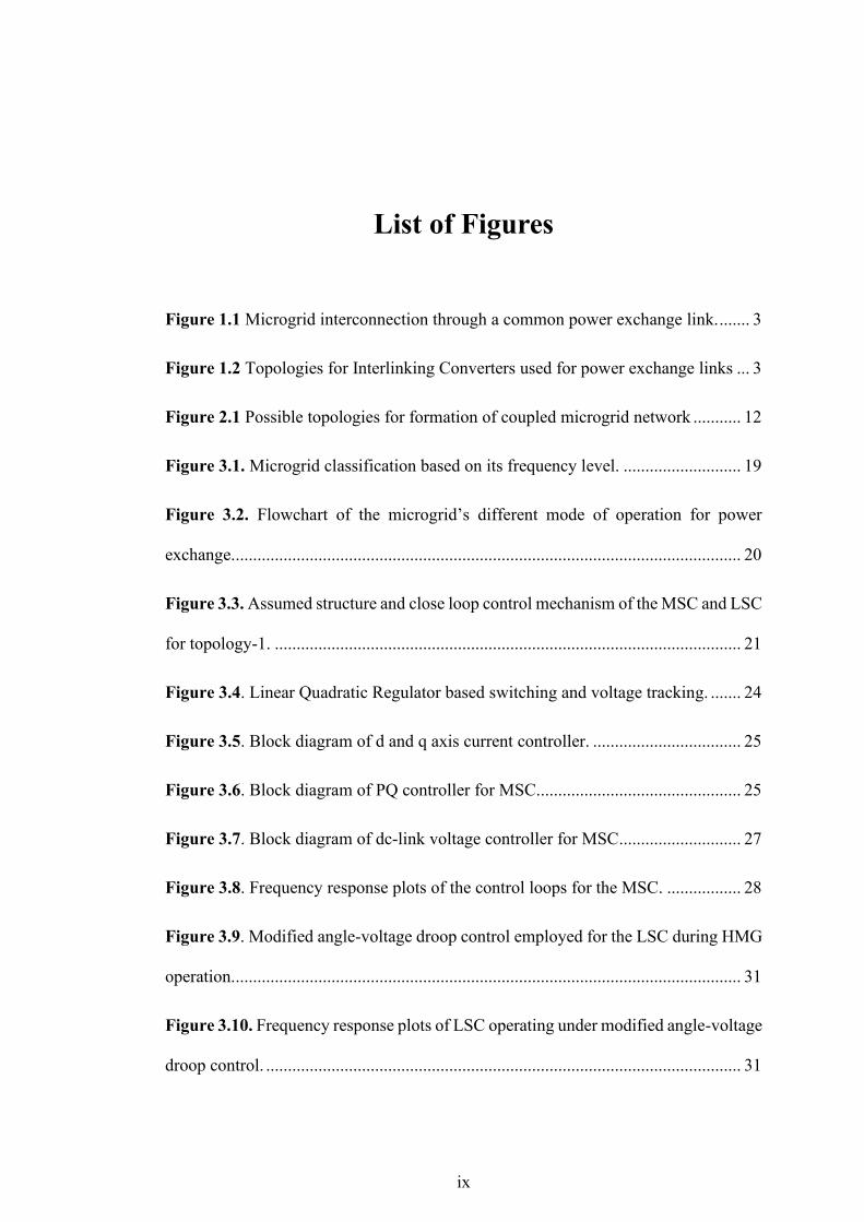
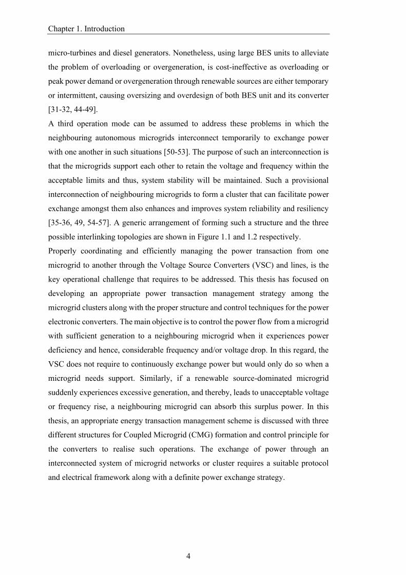
Figure 1.1 Microgrid interconnection through a common power exchange link.
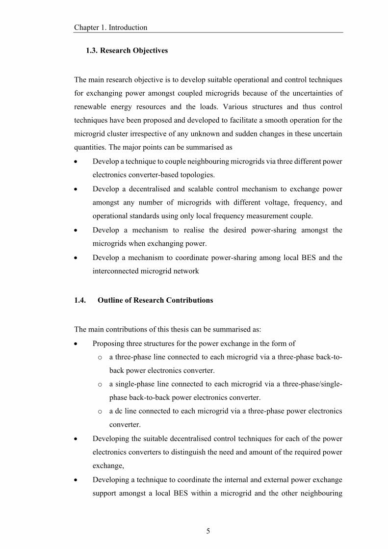
3ac
Topology-1
MSC LSC3
ac
3MSC LSC
1acac
3VSC dcac
Topology-2
Topology-3
Figure 1.2 Topologies for Interlinking Converters used for power exchange links
a further increase in the projects’ initial capital costs by either overdesigning and
oversizing the distributed generators or installation of large-scale energy storage
systems [4-6, 43-44, 48]. The problems of over-generation or overloading can be
effectively alleviated using oversized energy storage systems, but it will increase the
installation and operational costs of the microgrids [44-48]. Regardless of its cost,
floating Battery Energy Storage (BES) units are used conventionally and are
considered the most practical approach to support microgrids [49]. Such battery units,
controller through power electronics-based converters, can play an essential role
during peak demand, power deficiency, or overloading as they can respond faster than
Chapter 1. Introduction
4
micro-turbines and diesel generators. Nonetheless, using large BES units to alleviate
the problem of overloading or overgeneration, is cost-ineffective as overloading or
peak power demand or overgeneration through renewable sources are either temporary
or intermittent, causing oversizing and overdesign of both BES unit and its converter
[31-32, 44-49].
A third operation mode can be assumed to address these problems in which the
neighbouring autonomous microgrids interconnect temporarily to exchange power
with one another in such situations [50-53]. The purpose of such an interconnection is
that the microgrids support each other to retain the voltage and frequency within the
acceptable limits and thus, system stability will be maintained. Such a provisional
interconnection of neighbouring microgrids to form a cluster that can facilitate power
exchange amongst them also enhances and improves system reliability and resiliency
[35-36, 49, 54-57]. A generic arrangement of forming such a structure and the three
possible interlinking topologies are shown in Figure 1.1 and 1.2 respectively.
Properly coordinating and efficiently managing the power transaction from one
microgrid to another through the Voltage Source Converters (VSC) and lines, is the
key operational challenge that requires to be addressed. This thesis has focused on
developing an appropriate power transaction management strategy among the
microgrid clusters along with the proper structure and control techniques for the power
electronic converters. The main objective is to control the power flow from a microgrid
with sufficient generation to a neighbouring microgrid when it experiences power
deficiency and hence, considerable frequency and/or voltage drop. In this regard, the
VSC does not require to continuously exchange power but would only do so when a
microgrid needs support. Similarly, if a renewable source-dominated microgrid
suddenly experiences excessive generation, and thereby, leads to unacceptable voltage
or frequency rise, a neighbouring microgrid can absorb this surplus power. In this
thesis, an appropriate energy transaction management scheme is discussed with three
different structures for Coupled Microgrid (CMG) formation and control principle for
the converters to realise such operations. The exchange of power through an
interconnected system of microgrid networks or cluster requires a suitable protocol
and electrical framework along with a definite power exchange strategy.
Chapter 1. Introduction
5
1.3. Research Objectives
The main research objective is to develop suitable operational and control techniques
for exchanging power amongst coupled microgrids because of the uncertainties of
renewable energy resources and the loads. Various structures and thus control
techniques have been proposed and developed to facilitate a smooth operation for the
microgrid cluster irrespective of any unknown and sudden changes in these uncertain
quantities. The major points can be summarised as
• Develop a technique to couple neighbouring microgrids via three different power
electronics converter-based topologies.
• Develop a decentralised and scalable control mechanism to exchange power
amongst any number of microgrids with different voltage, frequency, and
operational standards using only local frequency measurement couple.
• Develop a mechanism to realise the desired power-sharing amongst the
microgrids when exchanging power.
• Develop a mechanism to coordinate power-sharing among local BES and the
interconnected microgrid network
1.4. Outline of Research Contributions
The main contributions of this thesis can be summarised as:
• Proposing three structures for the power exchange in the form of
o a three-phase line connected to each microgrid via a three-phase back-to-
back power electronics converter.
o a single-phase line connected to each microgrid via a three-phase/single-
phase back-to-back power electronics converter.
o a dc line connected to each microgrid via a three-phase power electronics
converter.
• Developing the suitable decentralised control techniques for each of the power
electronics converters to distinguish the need and amount of the required power
exchange,
• Developing a technique to coordinate the internal and external power exchange
support amongst a local BES within a microgrid and the other neighbouring
Chapter 1. Introduction
6
microgrids,
• Validating the robustness of the proposed power exchange topologies and
control techniques through stability and sensitivity analysis.
1.5. Organisation of the Thesis
The remainder of the thesis is organised as follows:
Chapter 2 surveys the relevant literature and critically analyses them to demonstrate
the research problems and possible solutions. Chapter 3 introduces suitable topologies
and presents the developed decentralised control mechanisms to realise power
exchange amongst the interconnected neighbouring microgrids. Chapter 4 presents
sample time-domain analysis results using the PSIM® simulation tool to demonstrate
and validate the proposed power exchange mechanism for all introduced topologies.
Chapter 5 discusses the stability of the proposed controllers while Chapter 6
evaluates the sensitivity and robustness of the proposals. Finally, Chapter 7 highlights
the key research findings and summarises the significant contributions of the thesis.
This chapter also proposes probable future directions in this research field.
Chapter 2. Literature Review
7
Chapter 2 Literature review
In this chapter, the operation and control principles of the interconnected microgrids
have been discussed and reviewed, and the different techniques suggested and
employed in the literature are surveyed. The chapter has first discussed the problems
associated with autonomous remote area microgrids and hence the coupling of such
neighbouring microgrids are proposed as a solution. Then, existing works on the
control and coupling of such microgrids as well as their architecture and stability, are
critically reviewed. This chapter also identifies the research gaps and suggests possible
techniques to address those research problems.
2.1. Operation of an Autonomous Microgrid
In the autonomous or islanded mode, microgrids are usually operated under droop
control to realise the desired power-sharing amongst the Distributed Energy Resources
(DER) while the voltage and frequency are regulated. by one or more of the DERs.
Thus, the active and reactive power must be continuously controlled at the output of
each droop-controlled DER to regulate the MG’s frequency and voltage within the
desired (acceptable) limits to ensure system stability [4-5].
Let us consider a network of Figure 1.1 where N autonomous microgrids, each
consisting of several DERs, distributed generators, loads, and one interlinking
converter coupled to a power exchange link. The interlinking converter can be any one
of the three topologies shown in Figure 1.2. The DERs are connected to the microgrid
through VSCs which are controlled in different operating modes to regulate the power
and frequency of each microgrid. The DERs are assumed to be operating in the 𝑃 − 𝑓
and 𝑄 − 𝑉 droop control mode, where the voltage and frequency at the output of each
DER is determined from [8-10]
Chapter 2. Literature Review
8
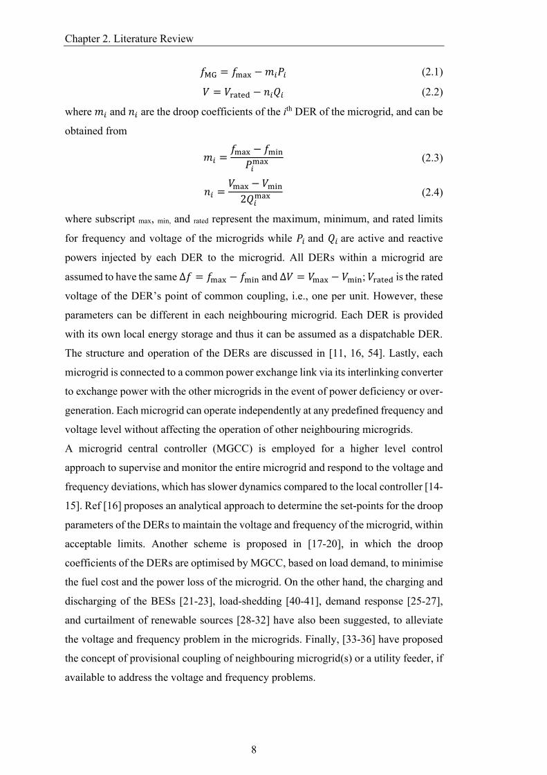
𝑓MG = 𝑓max − 𝑚𝑖𝑃𝑖 (2.1)
𝑉 = 𝑉rated − 𝑛𝑖𝑄𝑖 (2.2)
where 𝑚𝑖 and 𝑛𝑖 are the droop coefficients of the ith DER of the microgrid, and can be
obtained from
𝑚𝑖 =𝑓max − 𝑓min
𝑃𝑖max (2.3)
𝑛𝑖 =𝑉max − 𝑉min
2𝑄𝑖max (2.4)
where subscript max, min, and rated represent the maximum, minimum, and rated limits
for frequency and voltage of the microgrids while 𝑃𝑖 and 𝑄𝑖 are active and reactive
powers injected by each DER to the microgrid. All DERs within a microgrid are
assumed to have the same ∆𝑓 = 𝑓max − 𝑓min and ∆𝑉 = 𝑉max − 𝑉min; 𝑉rated is the rated
voltage of the DER’s point of common coupling, i.e., one per unit. However, these
parameters can be different in each neighbouring microgrid. Each DER is provided
with its own local energy storage and thus it can be assumed as a dispatchable DER.
The structure and operation of the DERs are discussed in [11, 16, 54]. Lastly, each
microgrid is connected to a common power exchange link via its interlinking converter
to exchange power with the other microgrids in the event of power deficiency or over-
generation. Each microgrid can operate independently at any predefined frequency and
voltage level without affecting the operation of other neighbouring microgrids.
A microgrid central controller (MGCC) is employed for a higher level control
approach to supervise and monitor the entire microgrid and respond to the voltage and
frequency deviations, which has slower dynamics compared to the local controller [14-
15]. Ref [16] proposes an analytical approach to determine the set-points for the droop
parameters of the DERs to maintain the voltage and frequency of the microgrid, within
acceptable limits. Another scheme is proposed in [17-20], in which the droop
coefficients of the DERs are optimised by MGCC, based on load demand, to minimise
the fuel cost and the power loss of the microgrid. On the other hand, the charging and
discharging of the BESs [21-23], load-shedding [40-41], demand response [25-27],
and curtailment of renewable sources [28-32] have also been suggested, to alleviate
the voltage and frequency problem in the microgrids. Finally, [33-36] have proposed
the concept of provisional coupling of neighbouring microgrid(s) or a utility feeder, if
available to address the voltage and frequency problems.
Chapter 2. Literature Review
9
2.2. Overloading and Excessive Generation in Microgrids
The trend of an islanded microgrid in remote localities or the regional edge-of-the-grid
network is gaining popularity due to its economical aspects and advantages. Several
studies have shown that employing autonomous microgrids is a feasible solution for
the electrification of remote areas as it can significantly reduce the levelised cost of
power generation [4-8, 37-38]. microgrids are cost-effective solutions than lengthy
transmission and distribution lines when it comes to the electrification of remote and
regional areas. Hence, a microgrid operating permanently in the autonomous mode can
be considered for such areas. Such microgrids will be mostly dominated by renewable
energy sources along with some diesel/gas-driven synchronous generators. High on-
going fuel cost and its transportation impose further challenges for the operation of
such MGs. At the same time, due to high intermittency and variability issues associated
with renewable energy sources, phenomena such as overloading and over-generation
can be seen in such microgrids, regardless of the considerations at the design stage
[38-44]. Overloading refers to the provisional deficiency in the microgrid’s generation
capability compared to its total demand, following which, load-shedding is the most
common and simple mechanism to alleviate the problem and return the voltage and
frequency to the acceptable limits. On the other hand, over-generation refers to the
situation in which the microgrid experiences high generation and an excess of power
through one or more of its non-dispatchable DERs [38-41]. Curtailing such renewable
energy resources is a solution to such conditions. However, both load-shedding and
curtailing renewable sources are uneconomical and undesirable which reduces the
reliability and resiliency of the system [42-44]. Proper risk-based planning can help to
prevent such scenarios by overdesigning and oversizing the DGs and/or using large-
scale energy storage systems to effectively mitigate the overloading and over-
generation problems and the corresponding voltage and frequency issues. However,
this will incur large installation and operational costs [3-4, 45-48]. Hence, the third
mode of operation has been proposed for microgrids in [35-36, 49-55] in which the
neighbouring microgrids can temporarily interconnect with each other during such
situations to support each other and to retain the frequency and voltage within the
desired limits and ensure the system stability. Note that, this interconnection is not to
a grid but to another neighbouring MG, which is also operating autonomously. This
system of interconnected autonomous microgrids is referred to as coupled microgrids

Chapter 2. Literature Review
10
(CMGs) in the remainder of this paper. Connecting a microgrid to its neighbouring
microgrids through a physical link is an effective operational strategy during power
deficiency or surplus [51-53]. Thus, the provision of forming CMGs improves and
enhances system reliability [22-24, 54-55].
2.3. Coupling of Autonomous Microgrids
In the future, it is expected that a remote locality will consist of several neighbouring
microgrids within a geographical area. Under the above assumptions, the overloading
or over-generation management strategy can be realised by properly interconnecting
two or more of those neighbouring microgrids. a suitable power deficiency or surplus
mitigation strategy can be instigated by suitably coupling two or more of those
microgrids [34-35, 49-55]. The CMG model and its operation based on the availability
of communication infrastructure and the concept of the power market is discussed in
ref [50, 56-57]. According to this concept, a common power exchange link (i.e.,
distribution lines) that enables a physical connection among the microgrids will be
introduced to interconnect the neighbouring microgrids. Such an interconnecting link
can be in either form of ac or dc [49, 55, 61-64]. A direct ac-ac connection between a
microgrid and the power exchange line can be easily realised through a conventional
circuit breaker or an interconnecting static switch which is very economical to a large
extent [60]. However, the structure and control mechanism of each microgrid can be
different from its neighbouring microgrids and such a direct ac-ac connection will
reduce the autonomy of their operations. In order to add proper isolation amongst the
microgrids to retain the autonomy in their operation, the power electronic converter-
based interlinking structure [65-66] will enable every microgrid to function
independently and autonomously, as well as facilitate power exchange with the
neighbouring microgrids [36, 60-62]. Power-sharing between two islanded microgrids
during mutual contingency is studied in [54, 59], whereas an autonomous control
approach to sharing power with neighbouring microgrids through a back-to-back
converter in the presence of a utility grid is proposed in [36, 61]. Neighbouring
microgrids can also interconnect to support each other during the occurrence of fault
leading to the outage of a section [67] or during normal conditions to minimise the
levelised cost of electricity [68]. If one of the microgrids temporarily observes a high-
Chapter 2. Literature Review
11
power generation by one of its DERs, the other neighbouring microgrid(s) can get
interconnected to one another to import power and thus offers electricity at a lower
price. A transformative architecture is proposed for coupling the nearby microgrids is
to improve the system resiliency during faults [69]. Ref [70-71] analyses the reliability
aspects of a CMG, while the voltage and current controllability in CMGs is analysed
in [72]. The dynamic operation of DERs within CMGs is investigated in [73] whereas
[74] examines the dynamic security of the CMGs. Several structures to form such
CMG, as well as its control mechanism are proposed in literature.
2.4. Structure and Control of Coupled Microgrids
Detailed analysis of different topologies and architectures of forming CMGs is shown
in [56-57, 75]. Optimal control of a utility grid-connected CMG is studied in [36, 66],
while an interactive control method to share the load in a CMG ensuring a wide range
of system stability is shown in [76-82]. An optimization-based technique is developed
in [83-85] to ensure optimal power exchange between the microgrids. A decision-
making-based approach is proposed to determine the most suitable microgrid(s) to
connect with an overloaded microgrid, based on different criteria such as available
surplus power, electricity cost, reliability and the distance of the neighbouring
microgrids as well as the voltage/frequency deviation in the CMG [86-88]. The
ultimate objective is that a microgrid can be coupled to any other microgrid (and not
necessarily an adjacent microgrid) if a general link is available to act as a power
exchange highway [55-56, 75, 89]. Figure 2.1 shows some of the possible
interconnection topologies of CMGs where the dashed lines mark the boundary of the
microgrids and solid lines represent the interconnecting links amongst them. Back-to-
back power electronic converter-based interface has been proposed in [35, 54, 90-91]
that can be used between each microgrid and the interconnecting three-phase ac line
to ensure autonomy in its operation. Such a scheme is comparatively expensive as two
voltage source converters (VSCs) are employed for every microgrid. However, the
main objective of such a connection is to provide isolation between the microgrids and
thus, microgrids with different operational regulations can exchange power while
being isolated through the dc-links within the back-to-back converters [35, 91].
Furthermore, such an interconnecting link can also be realised through a single-phase
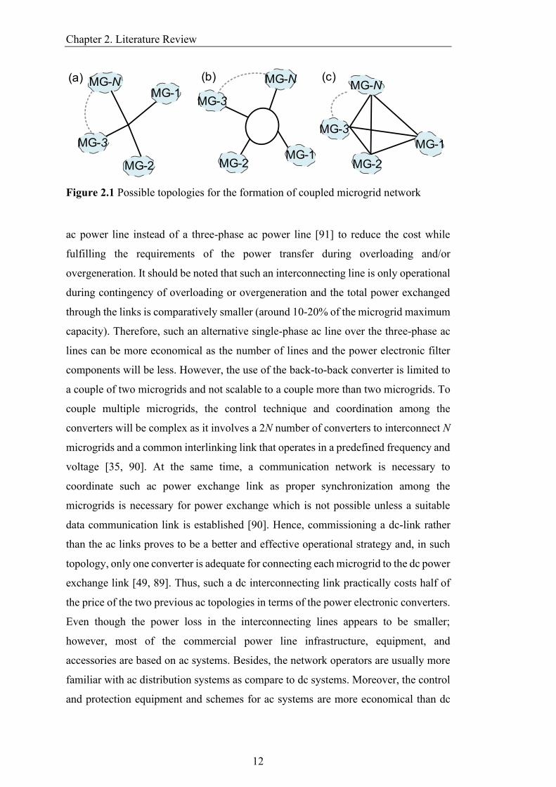
Chapter 2. Literature Review
12
MG-N(a)
MG-3
MG-1
(b) (c)
MG-2
MG-N
MG-3
MG-1MG-2
MG-N
MG-3
MG-1
MG-2
Figure 2.1 Possible topologies for the formation of coupled microgrid network
ac power line instead of a three-phase ac power line [91] to reduce the cost while
fulfilling the requirements of the power transfer during overloading and/or
overgeneration. It should be noted that such an interconnecting line is only operational
during contingency of overloading or overgeneration and the total power exchanged
through the links is comparatively smaller (around 10-20% of the microgrid maximum
capacity). Therefore, such an alternative single-phase ac line over the three-phase ac
lines can be more economical as the number of lines and the power electronic filter
components will be less. However, the use of the back-to-back converter is limited to
a couple of two microgrids and not scalable to a couple more than two microgrids. To
couple multiple microgrids, the control technique and coordination among the
converters will be complex as it involves a 2N number of converters to interconnect N
microgrids and a common interlinking link that operates in a predefined frequency and
voltage [35, 90]. At the same time, a communication network is necessary to
coordinate such ac power exchange link as proper synchronization among the
microgrids is necessary for power exchange which is not possible unless a suitable
data communication link is established [90]. Hence, commissioning a dc-link rather
than the ac links proves to be a better and effective operational strategy and, in such
topology, only one converter is adequate for connecting each microgrid to the dc power
exchange link [49, 89]. Thus, such a dc interconnecting link practically costs half of
the price of the two previous ac topologies in terms of the power electronic converters.
Even though the power loss in the interconnecting lines appears to be smaller;
however, most of the commercial power line infrastructure, equipment, and
accessories are based on ac systems. Besides, the network operators are usually more
familiar with ac distribution systems as compare to dc systems. Moreover, the control
and protection equipment and schemes for ac systems are more economical than dc
Chapter 2. Literature Review
13
systems to some extent. Properly coordinating and efficiently managing the power
transaction from one microgrid to another through the VSCs and lines, is the main
challenge that requires to be addressed. transaction management scheme is discussed
with three different structures for CMG
formation and control principle for the converters to realise such operations. The
exchange of power through an interconnected system of microgrid networks requires
a suitable protocol and electrical framework along with a definite power exchange
strategy. At the same time, stability of the CMG network must be ensured as, such an
interconnection may lead to system oscillation which may cause shut down of entire
network due to instability.
2.5. Stability of Coupled Microgrids
Prior to form a coupled microgrid network, the stability of the newly formed network
needs to be examined to avoid any instability of the system. For this purpose,
eigenvalue based small signal stability analysis is proposed in [47-48, 76]. It has been
shown in [77] that, the number of inertial and non-inertial DGs, their ratings, loads
need to be evaluated to ensure the stability of the CMG. Ref [78] further expands and
investigates the influence of the number of microgrids as well as the length and X/R
ratio of lines. Ref [79] suggests a decision-making function along with a small signal
stability evaluation prior to any transformation in the architecture of the CMG.
If properly designed, it is shown in [78-79] that, loci of the eigenvalue of the new CMG
network, is approximately within the same operating point eigenvalues of each
microgrid, when operating independently. Also, a sensitivity analysis is performed
along with stability analysis in [80] which reveals that microgrid with smaller stability
margins can cause a drop in the overall system stability margins of the other microgrids
after they are coupled.
It has also been reported that stability margins of the CMG can be strongly affected by
the DER nominal power while no significant effect was observed for the load demand
and power factor. Also, it is observed that the length and X/R ratio of the lines of the
microgrids can affect stability. However, no impact was observed whether the
microgrids had a loop or radial configuration. It is also recommended that developing
a general stability guideline is not straightforward as the operation of CMG depends
Chapter 2. Literature Review
14
on the conditions of the newly created system. Ref [79, 81-82] used Monte Carlo
simulations, to examine the network characteristics and the topology that can affect
the small-signal stability of a converter-dominated microgrid. It is found that simple
radial topologies are the most stable, though it is less resilient to faults and reduces the
network reliability. As the level of meshing is increased, the less stable the network
becomes. Hence it is recommended to keep the network topology as simple as possible
and operate the CMG in a ring configuration with a tie-open point. The study also
demonstrates that if the two adjacent converters tied with a smaller impedance line can
adversely affect the stability margin. As a result, it is recommended to connect adjacent
converters with enough electrical decoupling or isolation from each other to avoid
unstable interactions. Also, it was revealed that the length of the lines of the adjacent
microgrid can affect the stability margins of the CMG [80]. Based on stability studies,
the most optimum and robust topology to form the CMG can be selected.
2.6. Topology Comparison for Coupled Microgrids
Realising power exchange among multiple microgrids requires a predefined
coordinated control mechanism. It is possible to couple multiple microgrids to form
CMG using single-phase ac lines. The purpose of using a single-phase power exchange
link is to reduce the number of converter components and transmission lines in the
CMG network to make the system more economical. However, the line power loss is
higher in a single-phase link than that of a three-phase link for the same operating
conditions and power. Also, the power quality is poorer as single-phase instantaneous
power is oscillatory in nature. Hence, the three-phase power exchange link is superior
in every aspect as compared to the single-phase link unless a very small amount of
power is required to be exchanged within the CMG network through short
interconnecting lines. Though the number of components and power lines require for
the three-phase link are more, the power quality and performance are superior and
produce significantly lower line loss and thus, makes the system more efficient. At the
same time, the three-phase network exhibits larger system damping and hence, a better
stability margin as can be seen from the stability analysis [91-92].
On the other hand, CMG formed using dc interconnecting lines outperform any types
of ac links in terms of technical and economic aspects. However, there are several
Chapter 2. Literature Review
15
critical issues with dc power exchange links such as lack of proper standard and
guidelines for protection scheme, expensive protection equipment, larger fault current
level, arching during fault current interruption as no natural zero current crossings,
lower fault ride-through capability [91-93], circulating current in the network due to
unequal line resistance [94-95] and inaccurate and less efficient power-sharing based
on droop control technique [91-92]. On the other hand, the standard and infrastructure
for ac power transmission and distribution systems are well established and most of
the commercially available equipment are ac network-based which makes most of the
network operators prefer ac transmission systems over dc. Considering the cost and
complexity of the protection scheme, dc interconnecting link is more suitable when
the distance among the microgrids is longer. But as the distance among the microgrids
are increased (i.e. the line resistance is increased), the property of power-sharing based
on the droop control technique deteriorates and eventually diminishes. At the same
time, the increased value of line resistance makes the CMG network’s performance
highly sluggish [91]. Also, unequal line resistances can cause circulating current inside
the CMG network [94]. However, these problems can be addressed using the technique
discussed in [95], but the performance is not as satisfactory as the ac droop control
technique. In this paper where a three-phase ac interconnecting link is proposed to
form the CMG network, a modified virtual impedance-based angle-active power, and
voltage-reactive power droop control technique is employed that can successfully
address all the above-mentioned problems and the relevant results are shown in the
sensitivity analysis section of the paper. Hence, it can be concluded that the
performance of a CMG network formed using three-phase ac or dc interconnecting
lines, are comparable in terms of different technical and economic aspects and thus, a
proper techno-economical evaluation and optimization is required before selecting the
most suitable topology based on the type of microgrids to be interconnected, amount
of exchanged power, the duration and intervals at which power is going to be
exchanged, protection scheme and finally, the distance among them. A comparative
review of ac and dc technology used in microgrid application can be found in [91-92].
It was discussed in [91] that, though in theory dc systems are more advantageous in
several aspects, however, considering the present power transmission infrastructure,
commercially available protection equipment, technical constraints, network
standards, and guidelines, ac systems are still more economical
To address the above research gaps, this thesis presents a fully decentralised approach
Chapter 2. Literature Review
16
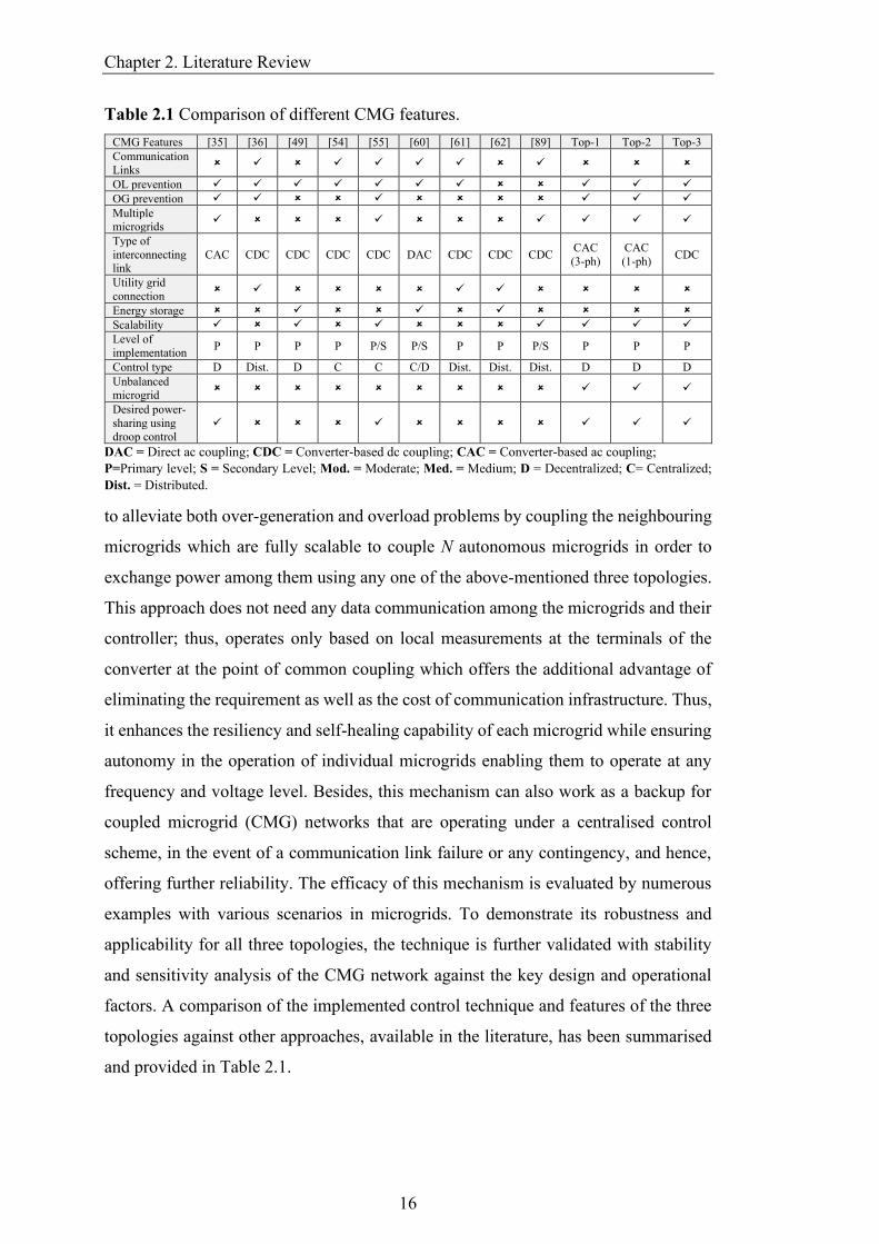
Table 2.1 Comparison of different CMG features.
CMG Features [35] [36] [49] [54] [55] [60] [61] [62] [89] Top-1 Top-2 Top-3
Communication
Links
OL prevention
OG prevention
Multiple microgrids
Type of
interconnecting link
CAC CDC CDC CDC CDC DAC CDC CDC CDC CAC
(3-ph)
CAC
(1-ph) CDC
Utility grid
connection
Energy storage
Scalability
Level of
implementation P P P P P/S P/S P P P/S P P P
Control type D Dist. D C C C/D Dist. Dist. Dist. D D D
Unbalanced
microgrid
Desired power-
sharing using
droop control
DAC = Direct ac coupling; CDC = Converter-based dc coupling; CAC = Converter-based ac coupling;
P=Primary level; S = Secondary Level; Mod. = Moderate; Med. = Medium; D = Decentralized; C= Centralized;
Dist. = Distributed.
to alleviate both over-generation and overload problems by coupling the neighbouring
microgrids which are fully scalable to couple N autonomous microgrids in order to
exchange power among them using any one of the above-mentioned three topologies.
This approach does not need any data communication among the microgrids and their
controller; thus, operates only based on local measurements at the terminals of the
converter at the point of common coupling which offers the additional advantage of
eliminating the requirement as well as the cost of communication infrastructure. Thus,
it enhances the resiliency and self-healing capability of each microgrid while ensuring
autonomy in the operation of individual microgrids enabling them to operate at any
frequency and voltage level. Besides, this mechanism can also work as a backup for
coupled microgrid (CMG) networks that are operating under a centralised control
scheme, in the event of a communication link failure or any contingency, and hence,
offering further reliability. The efficacy of this mechanism is evaluated by numerous
examples with various scenarios in microgrids. To demonstrate its robustness and
applicability for all three topologies, the technique is further validated with stability
and sensitivity analysis of the CMG network against the key design and operational
factors. A comparison of the implemented control technique and features of the three
topologies against other approaches, available in the literature, has been summarised
and provided in Table 2.1.

Chapter 2. Literature Review
17
2.7. Summary
This chapter has surveyed different control techniques proposed in the literature to
alleviate the overloading and excessive generation in an autonomous microgrid. The
research gaps in the field and several proposed techniques to address those gaps are
identified. Based on this literature review, suitable topologies are chosen, and proper
control mechanisms have been developed and formulated, which are introduced and
discussed in the next chapter. These methods can alleviate the overloading and
excessive generation in autonomous microgrids and thus can improve the voltage and
frequency quality by coupling a microgrid in problem to one or more of its
neighbouring microgrids and coordinate power-sharing within its local BES. The
proposed techniques overcome the limitations of the existing similar techniques in the
literature and more generalised to couple any number of microgrids.

Chapter 3. Operational and Control Technique
18
Chapter 3 Operational and Control
Technique
This chapter presents the four proposed decentralised power exchange techniques and
topologies for CMG operation. The proposed techniques and topologies are (a)
Topology-1: three-phase ac power exchange link, (b) Topology-2: single-phase ac
power exchange link, (c) Topology-3: dc power exchange link, and (d) Coordinated
control and power-sharing mechanism among BES and CMGs.
3.1 Microgrid Classification
This provisional power exchange mechanism can be realised by interconnecting the
neighbouring microgrids to a common power exchange link to facilitate power
exchange among the microgrids during an overload/excess generation. Thus, the
neighbouring microgrids can be coupled via a power electronic converter-based
interface and ac/dc interconnecting power lines to form a CMG. Such a strategy is
attained by monitoring and controlling the frequency of each microgrid. It is obvious
that autonomous microgrids are conventionally operating under droop control to share
power amongst their DERs and in such a control scheme, as the total load demand of
a microgrid increases, its frequency decreases, and vice versa. Such a distinct
behaviour can be used as an indication of the microgrid’s power shortage or surplus,
and hence, the approach eliminates the necessity of any sort of data communication
link or a centralised controller. The key benefit of this approach is that it eliminates
the necessity of installing and operating a communication infrastructure to enable the
microgrids to exchange power. It should be mentioned here, even in the presence of a
central controller with communication links to monitor and regulate the power
exchange, this approach can be implemented as the backup system that is activated in
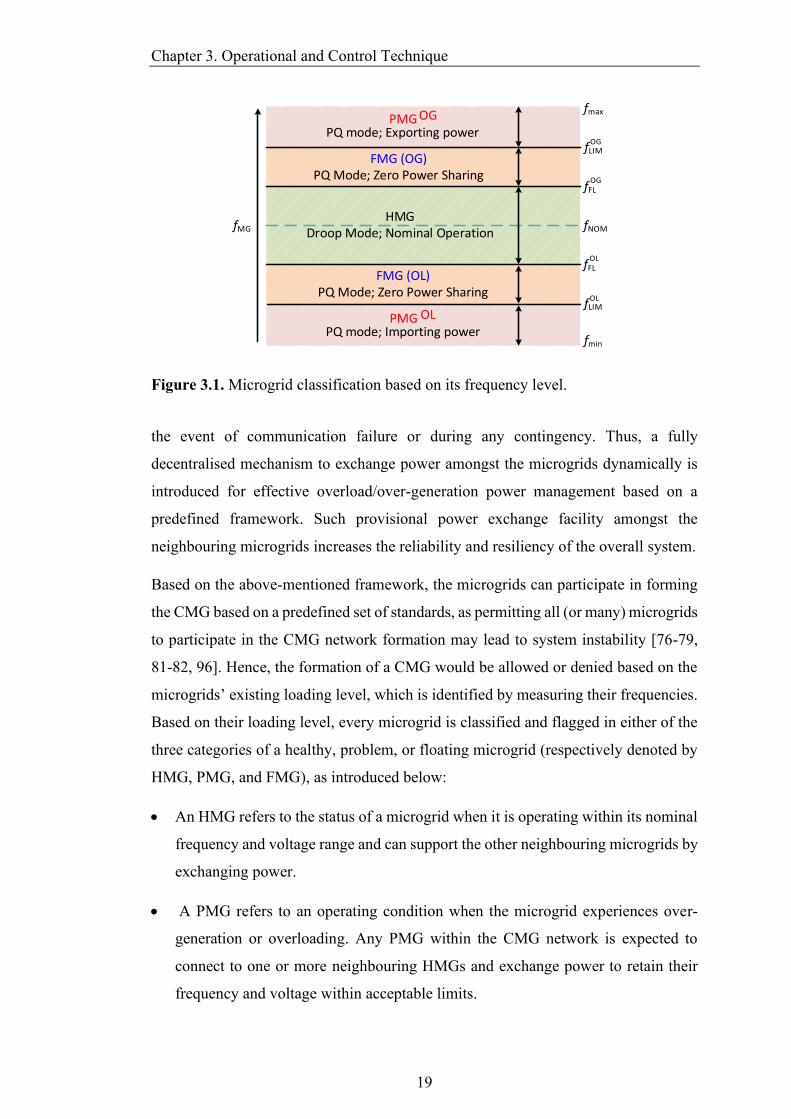
Chapter 3. Operational and Control Technique
19
HMG Droop Mode; Nominal Operation
FMG (OG)PQ Mode; Zero Power Sharing
PQ mode; Exporting power
fmax
fmin
fMG fNOM
OGPMG
FMG (OL)PQ Mode; Zero Power Sharing
PQ mode; Importing powerOLPMG
fLIM
fFLOL
fFL
fLIM
OL
OG
OG
Figure 3.1. Microgrid classification based on its frequency level.
the event of communication failure or during any contingency. Thus, a fully
decentralised mechanism to exchange power amongst the microgrids dynamically is
introduced for effective overload/over-generation power management based on a
predefined framework. Such provisional power exchange facility amongst the
neighbouring microgrids increases the reliability and resiliency of the overall system.
Based on the above-mentioned framework, the microgrids can participate in forming
the CMG based on a predefined set of standards, as permitting all (or many) microgrids
to participate in the CMG network formation may lead to system instability [76-79,
81-82, 96]. Hence, the formation of a CMG would be allowed or denied based on the
microgrids’ existing loading level, which is identified by measuring their frequencies.
Based on their loading level, every microgrid is classified and flagged in either of the
three categories of a healthy, problem, or floating microgrid (respectively denoted by
HMG, PMG, and FMG), as introduced below:
• An HMG refers to the status of a microgrid when it is operating within its nominal
frequency and voltage range and can support the other neighbouring microgrids by
exchanging power.
• A PMG refers to an operating condition when the microgrid experiences over-
generation or overloading. Any PMG within the CMG network is expected to
connect to one or more neighbouring HMGs and exchange power to retain their
frequency and voltage within acceptable limits.
Chapter 3. Operational and Control Technique
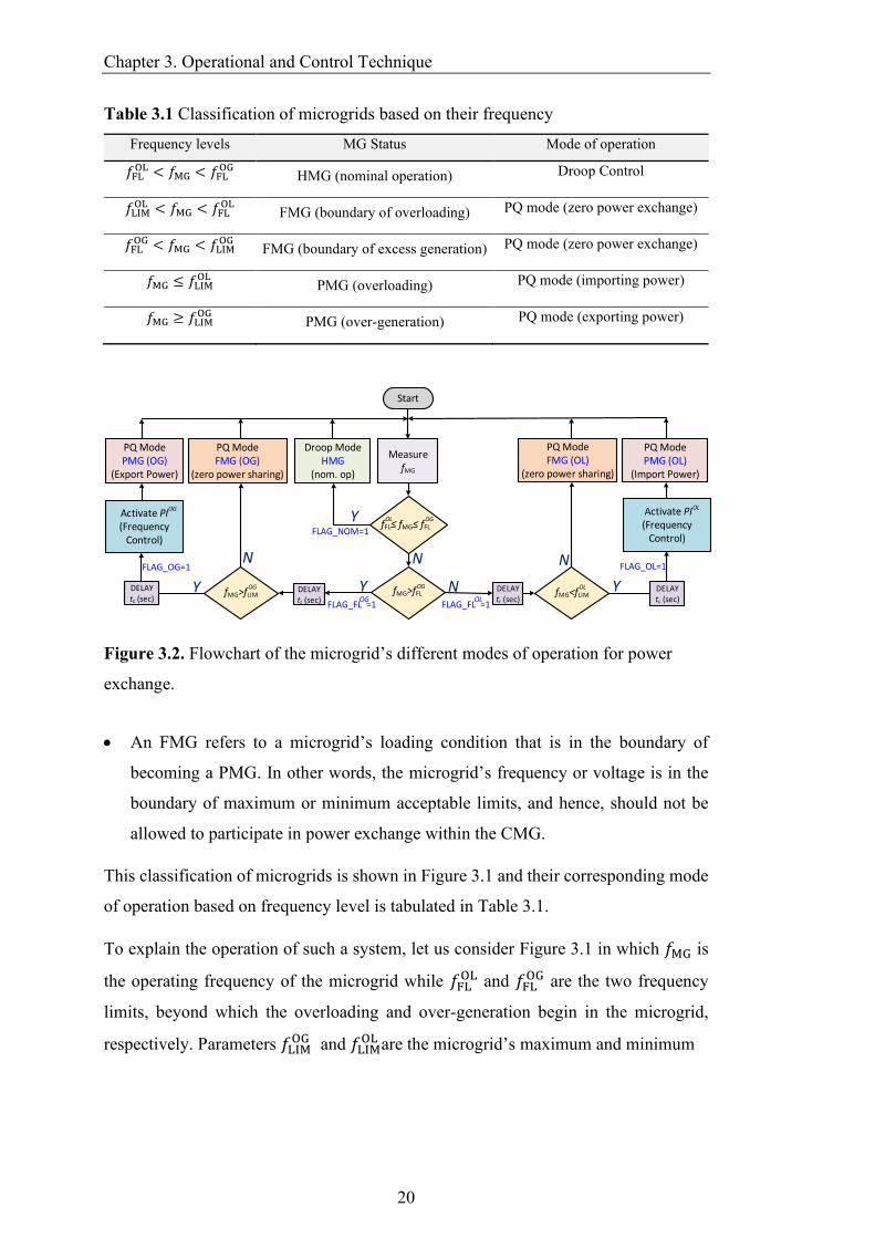
20
Table 3.1 Classification of microgrids based on their frequency
Frequency levels MG Status Mode of operation
𝑓FLOL < 𝑓MG < 𝑓FL
OG HMG (nominal operation) Droop Control
𝑓LIMOL < 𝑓MG < 𝑓FL
OL FMG (boundary of overloading) PQ mode (zero power exchange)
𝑓FLOG < 𝑓MG < 𝑓LIM
OG FMG (boundary of excess generation) PQ mode (zero power exchange)
𝑓MG ≤ 𝑓LIMOL PMG (overloading) PQ mode (importing power)
𝑓MG ≥ 𝑓LIMOG PMG (over-generation) PQ mode (exporting power)
Start
MeasurefMG
Droop ModeHMG
(nom. op)
DELAYtc (sec)
PQ ModePMG (OG)
(Export Power)
Activate PI(Frequency
Control)
PQ ModePMG (OL)
(Import Power)
Y
N
OL
FLAG_NOM=1
FLAG_OL=1
Activate PI(Frequency
Control)
OG
N DELAYtr (sec)
fFL fMG fFL OL OG
fMG>fFL OG
fMG<fLIM OL
PQ ModeFMG (OL)
(zero power sharing)
N
Y
N
DELAYtr (sec) FLAG_FL =1
OG
YfMG>fLIM OG
PQ ModeFMG (OG)
(zero power sharing)
DELAYtc (sec)
FLAG_OG=1
YFLAG_FL =1
OL
Figure 3.2. Flowchart of the microgrid’s different modes of operation for power
exchange.
• An FMG refers to a microgrid’s loading condition that is in the boundary of
becoming a PMG. In other words, the microgrid’s frequency or voltage is in the
boundary of maximum or minimum acceptable limits, and hence, should not be
allowed to participate in power exchange within the CMG.
This classification of microgrids is shown in Figure 3.1 and their corresponding mode
of operation based on frequency level is tabulated in Table 3.1.
To explain the operation of such a system, let us consider Figure 3.1 in which 𝑓MG is
the operating frequency of the microgrid while 𝑓FLOL and 𝑓FL
OG are the two frequency
limits, beyond which the overloading and over-generation begin in the microgrid,
respectively. Parameters 𝑓LIMOG and 𝑓LIM
OL are the microgrid’s maximum and minimum

Chapter 3. Operational and Control Technique
21
LSC
Rg Lg Rf LfCdc/2
MG
MSC
Cf
dc Link
LCL Filter
vg
igabc
if1abc
vc1abc
abc
Vdc
(Vdc )ref 2
Compensator PQ Controller
Pref
Qref
refvc1
vg
(.)2
(PLL)
vq vd
θg
iq id
ig
Power Controldc Voltage Control
+
3
3
Voltage Tracking
dq
abc abc
dq
3
if1
vc1
3LQR
switchingcontroller
Gate Pulses
6
+
Vdc
3- ph Power
exchange link
Voltage Tracking
LQRswitchingcontroller
Gate Pulses
6
3
3abc
abc
Reference Selection
Logic
fMG
vg1
fFL
fFL
PIPQ Controller Pref
Qref
(PLL)vqvd
θg
iqid
Frequency Control
Reset
dq
abc
dq
refvc2
ReferenceVoltage
Generation
|Vdr|
δdr
Droop Controller
Power Calculation
Pline
fLIMOG fLIM
OL
fFLOG
fFLOL
fMG
Droop Control
abc
abc
3
3
OG
OL
abc
3
3
vc_drref
vc_PQref
MUX+1
RgLgRfLf
Cf
LCLFilter
vline
ilineabcif2
abc
vc2abc
abc
if2abc
vc2abc
ilineabc
vlineabc
vlineabc
ilineabc3
3
Cdc/2
Qline
line
line
MG
line
TM1TM2TM3 TL1 TL2 TL3
BL1 BL2 BL3BM1BM2BM3
line
line
line line
a
Figure 3.3. Assumed structure and close loop control mechanism of the MSC and
LSC for topology-1.
permissible frequency to operate within the acceptable limit, while 𝑓max is the no-load
frequency and 𝑓min is the frequency where the microgrid becomes unstable due to
excessive loading. Referring to Figure 3.1 and Table 3.1, the microgrid’s operating
status can be denoted as:
• The microgrid is defined as HMG when 𝑓FLOL < 𝑓MG < 𝑓FL
OG.
• FMG can be attained in two conditions; i.e., when 𝑓LIMOL < 𝑓MG < 𝑓FL
OL (increasing
load demand) or 𝑓FLOG < 𝑓MG < 𝑓LIM
OG (decreasing load demand).
• PMG can be attained in two conditions; i.e., when 𝑓min < 𝑓MG < 𝑓LIMOL
(overloading) or 𝑓LIMOG < 𝑓MG < 𝑓max (over-generation).
Figure 3.2 demonstrates the steps of detecting the microgrid’s status and the operation
of the CMG to enable power exchange amongst the microgrids using a flowchart.
3.2 Various CMG structure and their control
The CMG formation among the neighbouring microgrids is achieved through power
electronics converters and interconnecting power lines using the three different
topologies. For topology-1 and 2, a back-to-back converter structure is employed
whereas, a single-stage converter is enough for topology-3. The converter connected
to the microgrid is labelled as the microgrid-side converter (MSC) while the other one
Chapter 3. Operational and Control Technique
22
is labelled as the line-side converter (LSC). In topology-1 and 2, both MSC and LSC
are voltage source converters (VSCs) connected back-to-back with each other via a
common dc-link to provide the isolation which enables the microgrids to operate with
full autonomy and no synchronization of MSC with LSC is required (see Figure 1.1).
In such an arrangement, MSC enables bi-directional power flow between the microgrid
and dc-link whereas, LSC enables bidirectional power flow between dc-link and the
interconnecting lines. In this approach, the purpose of MSC is to regulate only the dc-
link voltage; however, the mode of operation of LSC depends on the frequency (i.e.,
loading level) of the microgrid to which it is connected. On the other hand, in topology-
3, a single-stage voltage source converter is used to connect the dc power lines to the
microgrid and labelled as VSC (see Figure 1.2), which can operate either in dc droop
control mode or constant PQ control mode depending on the status of the microgrid.
3.2.1 Three-phase AC interconnection (Topology-1)
Topology-1 is a three-phase ac interconnecting line with two back-to-back connected
power electronic converters. In this topology, both the MSC and LSC are assumed to
be three-phase, three-leg VSC using IGBTs or MOSFETs. Each VSC is connected to
its point of common coupling through a three-phase LCL filter. The structures of MSC
and LSC are shown schematically in Figure 3.3. However, any other three-phase
topologies of VSCs can also be used instead of the considered topologies here.
3.2.1.1 Control of MSC
The main function of MSC is to regulate and maintain the dc-link voltage of 𝑉dc at the
desired reference level of 𝑉dcref. This is valid for any status of the microgrid (i.e., HMG,
PMG, FMG). The dc-link will exchange the appropriate amount of power with the
microgrid through proper voltage regulation, such that the dc-link voltage remains
constant. This can be realised through a closed-loop control mechanism (i.e., the
outermost loop in the MSC part of Figure 3.3) to determine the reference active power
(𝑃ref) that should be drawn from or injected into the microgrid to avoid a deviation in
𝑉dc. The MSC is not likely to exchange any reactive power with the microgrid and
hence, the reference for reactive power (𝑄ref ) is assumed to be zero. Based on these
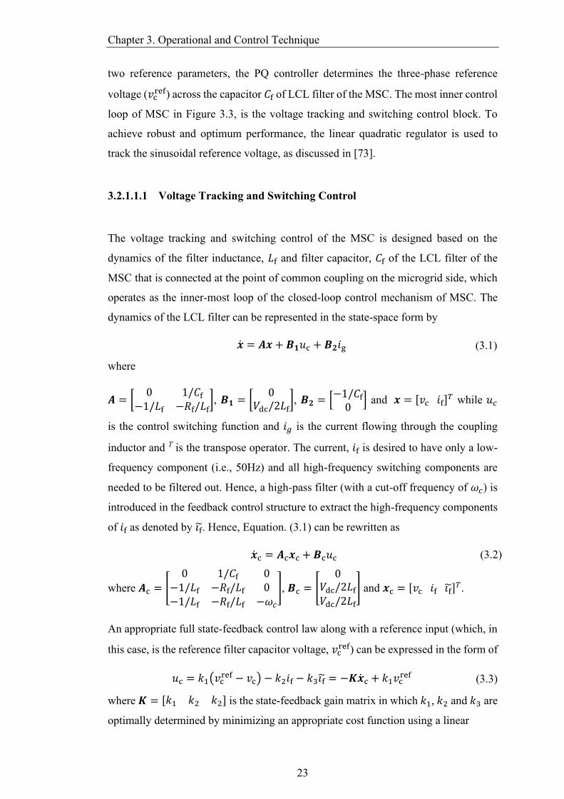
Chapter 3. Operational and Control Technique
23
two reference parameters, the PQ controller determines the three-phase reference
voltage (𝑣cref) across the capacitor 𝐶f of LCL filter of the MSC. The most inner control
loop of MSC in Figure 3.3, is the voltage tracking and switching control block. To
achieve robust and optimum performance, the linear quadratic regulator is used to
track the sinusoidal reference voltage, as discussed in [73].
3.2.1.1.1 Voltage Tracking and Switching Control
The voltage tracking and switching control of the MSC is designed based on the
dynamics of the filter inductance, 𝐿f and filter capacitor, 𝐶f of the LCL filter of the
MSC that is connected at the point of common coupling on the microgrid side, which
operates as the inner-most loop of the closed-loop control mechanism of MSC. The
dynamics of the LCL filter can be represented in the state-space form by
= 𝑨𝒙 + 𝑩𝟏𝑢c + 𝑩𝟐𝑖g (3.1)
where
𝑨 = [0 1/𝐶f
−1/𝐿f −𝑅f/𝐿f], 𝑩𝟏 = [
0𝑉dc/2𝐿f
], 𝑩𝟐 = [−1/𝐶f
0] and 𝒙 = [𝑣c 𝑖f]
𝑇 while 𝑢𝑐
is the control switching function and 𝑖𝑔 is the current flowing through the coupling
inductor and T is the transpose operator. The current, 𝑖f is desired to have only a low-
frequency component (i.e., 50Hz) and all high-frequency switching components are
needed to be filtered out. Hence, a high-pass filter (with a cut-off frequency of 𝜔𝑐) is
introduced in the feedback control structure to extract the high-frequency components
of 𝑖f as denoted by 𝑖f. Hence, Equation. (3.1) can be rewritten as
c = 𝑨c𝒙c + 𝑩c𝑢c (3.2)
where 𝑨c = [
0 1/𝐶f 0−1/𝐿f −𝑅f/𝐿f 0−1/𝐿f −𝑅f/𝐿f −𝜔𝑐
], 𝑩c = [
0𝑉dc/2𝐿f
𝑉dc/2𝐿f
] and 𝒙c = [𝑣c 𝑖f 𝑖f]𝑇.
An appropriate full state-feedback control law along with a reference input (which, in
this case, is the reference filter capacitor voltage, 𝑣cref) can be expressed in the form of
𝑢c = 𝑘1(𝑣cref − 𝑣c) − 𝑘2𝑖f − 𝑘3𝑖f = −𝑲c + 𝑘1𝑣c
ref (3.3)
where 𝑲 = [𝑘1 𝑘2 𝑘2] is the state-feedback gain matrix in which 𝑘1, 𝑘2 and 𝑘3 are
optimally determined by minimizing an appropriate cost function using a linear
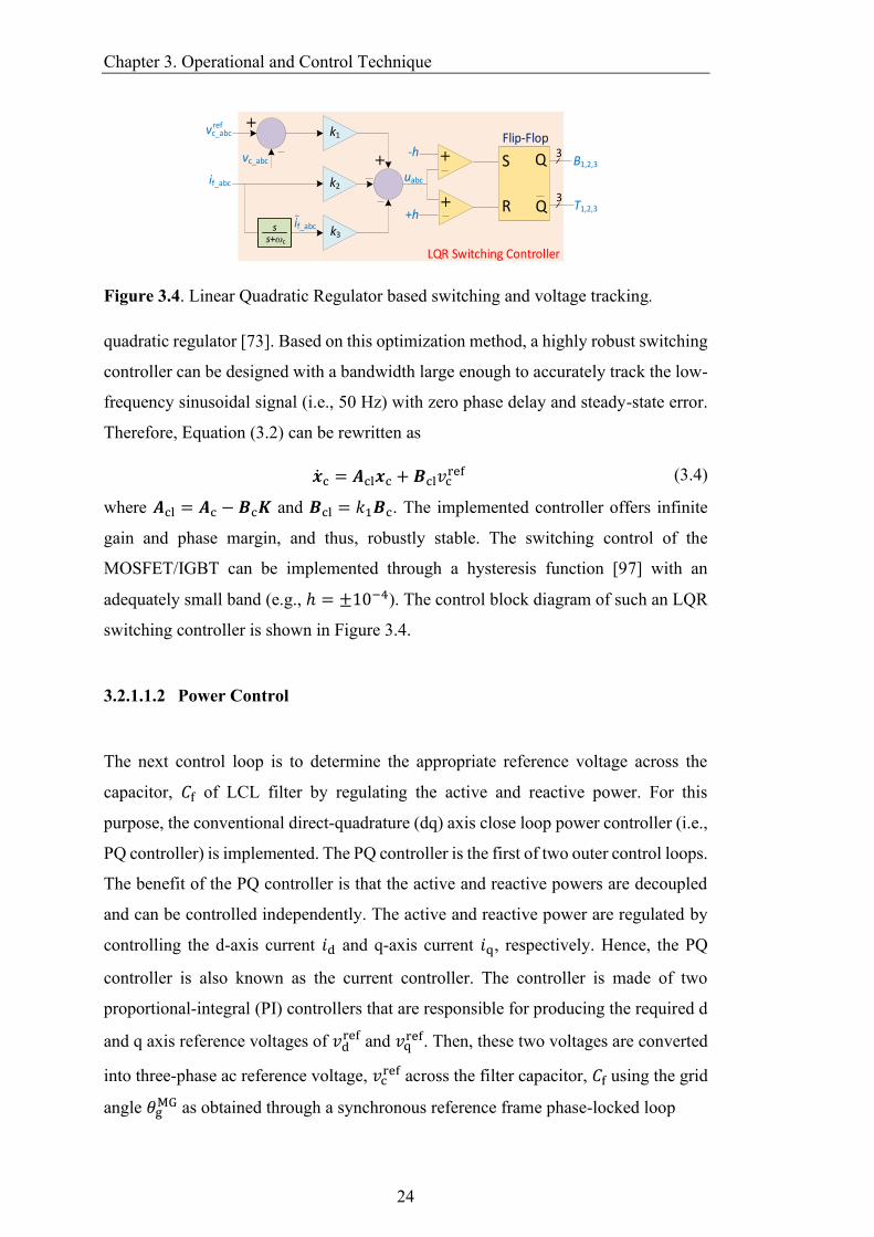
Chapter 3. Operational and Control Technique
24
+
+ R
S Q
Q
Flip-Flop+
vc_abc
if_abc
if_abc
k1
k2
k3
+-h
+h
uabc
vc_abc
~
ref
T1,2,3
B1,2,3
3
3
s+ωc
s
LQR Switching Controller
Figure 3.4. Linear Quadratic Regulator based switching and voltage tracking.
quadratic regulator [73]. Based on this optimization method, a highly robust switching
controller can be designed with a bandwidth large enough to accurately track the low-
frequency sinusoidal signal (i.e., 50 Hz) with zero phase delay and steady-state error.
Therefore, Equation (3.2) can be rewritten as
c = 𝑨cl𝒙c + 𝑩cl𝑣cref (3.4)
where 𝑨cl = 𝑨c − 𝑩c𝑲 and 𝑩cl = 𝑘1𝑩c. The implemented controller offers infinite
gain and phase margin, and thus, robustly stable. The switching control of the
MOSFET/IGBT can be implemented through a hysteresis function [97] with an
adequately small band (e.g., ℎ = ±10−4). The control block diagram of such an LQR
switching controller is shown in Figure 3.4.
3.2.1.1.2 Power Control
The next control loop is to determine the appropriate reference voltage across the
capacitor, 𝐶f of LCL filter by regulating the active and reactive power. For this
purpose, the conventional direct-quadrature (dq) axis close loop power controller (i.e.,
PQ controller) is implemented. The PQ controller is the first of two outer control loops.
The benefit of the PQ controller is that the active and reactive powers are decoupled
and can be controlled independently. The active and reactive power are regulated by
controlling the d-axis current 𝑖d and q-axis current 𝑖q, respectively. Hence, the PQ
controller is also known as the current controller. The controller is made of two
proportional-integral (PI) controllers that are responsible for producing the required d
and q axis reference voltages of 𝑣dref and 𝑣q
ref. Then, these two voltages are converted
into three-phase ac reference voltage, 𝑣cref across the filter capacitor, 𝐶f using the grid
angle 𝜃gMG as obtained through a synchronous reference frame phase-locked loop
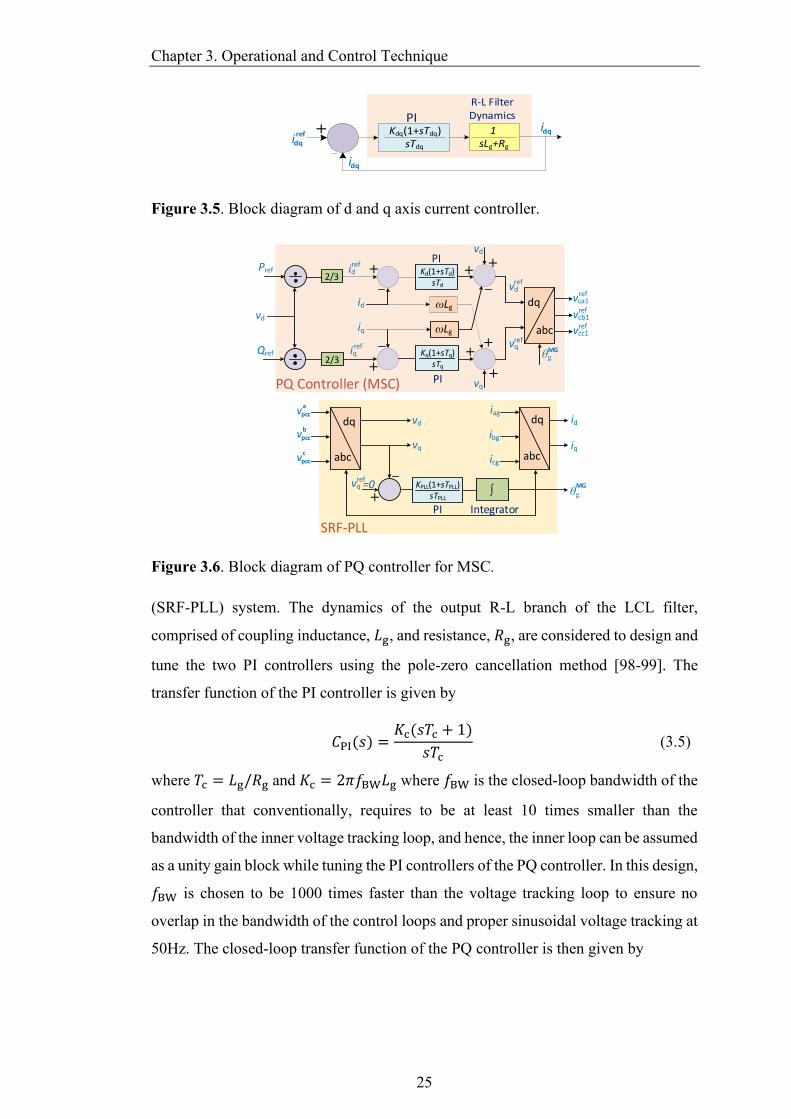
Chapter 3. Operational and Control Technique
25
idqref
idq
Kdq(1+sTdq)sTdq
PI 1
sLg+Rg
idq+
R-L FilterDynamics
Figure 3.5. Block diagram of d and q axis current controller.
Pref
Qref
id
iq
iqref
idref
vd
vq
vdref
vqref
abc
dq
vcc1ref
vcb1ref
vca1ref
vq
vd
vqref
=0
abc
dq dq
abc
id
iq
iag
ibg
icg
ωLg
ωLg
PQ Controller (MSC)
SRF-PLL
vd
Kd(1+sTd)sTd
Kq(1+sTq)sTq
+
+
++
++
+
θg
θg
vpcca
vpccb
vpccc
+
KPLL(1+sTPLL)sTPLL
PI Integrator
PI
PI
2/3
2/3
MG
MG
Figure 3.6. Block diagram of PQ controller for MSC.
(SRF-PLL) system. The dynamics of the output R-L branch of the LCL filter,
comprised of coupling inductance, 𝐿g, and resistance, 𝑅g, are considered to design and
tune the two PI controllers using the pole-zero cancellation method [98-99]. The
transfer function of the PI controller is given by
𝐶PI(𝑠) =𝐾c(𝑠𝑇c + 1)
𝑠𝑇c (3.5)
where 𝑇c = 𝐿g/𝑅g and 𝐾c = 2𝜋𝑓BW𝐿g where 𝑓BW is the closed-loop bandwidth of the
controller that conventionally, requires to be at least 10 times smaller than the
bandwidth of the inner voltage tracking loop, and hence, the inner loop can be assumed
as a unity gain block while tuning the PI controllers of the PQ controller. In this design,
𝑓BW is chosen to be 1000 times faster than the voltage tracking loop to ensure no
overlap in the bandwidth of the control loops and proper sinusoidal voltage tracking at
50Hz. The closed-loop transfer function of the PQ controller is then given by
Chapter 3. Operational and Control Technique
26
𝐺c(𝑠) =𝑖dq
ref
𝑖dq=
1
𝑠𝜏c + 1=
𝑃ref
𝑃s (3.6)
where 𝜏𝑐 = 𝐿g/𝐾𝑐 is the time constant of the current controller, 𝑃ref is the reference
power and 𝑃s is the active power output of the converter. It should be noted here, 𝑃ref
is generated through the outermost control loop i.e., the dc-link voltage controller. The
assumed close loop control block diagram of d and q axis current controller is shown
in Figure 3.5 while the PQ controller for MSC is shown in Figure 3.6.
3.2.1.1.3 DC-link Voltage Control
The outermost loop of the control structure is the dc-link voltage controller. The
dynamics of the voltage across the dc-link capacitor, 𝑉dc, with respect to converter
output power, 𝑃s, can be described in terms of a transfer function as [98, 100]
𝐺dc(𝑠) =𝑉dc
2
𝑃s= (
−2
𝐶dc)
(𝑠𝜏dc + 1)
𝑠 (3.7)
where 𝜏dc = 2(𝐿f + 𝐿g)𝑃so/3𝑉do2 . The transfer function of 𝐺dc(𝑠) is a linearised small-
signal model where 𝑃so is the steady-state power output of the converter and 𝑉do is the
d-axis steady-state voltage at the point of common coupling of the converter to the
microgrid. It is a non-minimum phase system with a right half plane zero, whose
location depends on the steady-state value of 𝑃so and 𝑉do. If these two parameters are
varied, then the controller needs to be redesigned to ensure the required stability
margin. In other words, the controllers are designed to exchange rated power at a
specific voltage level, and hence the exchanged power through the dc-link should not
exceed its maximum limit. In order to design a controller that regulates the dc-link
voltage with the required gain and phase margin to ensure satisfactory performance, a
type-2 controller can be designed. The generic transfer function of a type- 2 controller
can be written as
𝐶dc(𝑠) =𝐾dc(𝑠 + 𝜔z)
𝑠(𝑠 + 𝜔p) (3.8)
Such type of controller can be designed using the K-factor method, as described in
[102]. The closed-loop control system of the dc-link voltage can be realised by the
block diagram of Figure 3.7. It should be noted here that, while regulating the dc-link

Chapter 3. Operational and Control Technique
27
+
Vdc ref
( )2
DC link Compensator
Kdc(s+ωz)
s(s+ωp) (sτc +1)1 -2
Cdc
(sτdc +1)s
( )2Vdc
Power Controller Dynamics
DC linkDynamics
Pdc Ps
Figure 3.7. Block diagram of dc-link voltage controller for MSC.
voltage the reference power of 𝑃ref in Equation (3.6) is 𝑃dc (i.e., the power that needs
to be exchanged bi-directionally to keep the dc-link voltage fixed to its reference
value) as can be seen from Figure 3.7. As the voltage tracking loop is made almost
1000 times faster than the power control loop, the overall system dynamics of the dc-
link voltage can be assumed as
𝐺OL(𝑠) = 𝐺c(𝑠)𝐺dc(𝑠) = (−2
𝐶dc)
(𝑠𝜏dc + 1)
𝑠(𝑠𝜏c + 1) (3.9)
Hence, 𝐺OL(𝑠) is the open-loop transfer function assumed to apply the K-factor
method. The steps of designing the controller using this method are discussed in detail
in [100-101]. The close loop frequency responses of all the three control loops are
shown in Figure 3.8. The close loop bandwidths of voltage tracking, power, and dc-
link controller are 318kHz, 300Hz, and 20Hz, respectively.
3.2.1.2 Control of LSC
Two separate modes of operation for the LSC are considered that depend on the status
of the microgrid. It has been proposed that to form a CMG, the LSC of all HMGs
should operate under droop control mode to enable power-sharing, whereas the LSC
of the FMGs and PMGs should operate in constant power (PQ) control mode (Refer
to the flowchart of Figure 3.2). The LSCs connected to HMGs, form the CMG and
provide the required droop voltage and angle references that enable power-sharing
among the HMGs within a CMG, whereas it will absorb or inject the desired amount
of power from the interconnecting power lines to alleviate the overloading or over-
generation situations respectively when a microgrid becomes PMG.
To realise the above objective, the frequencies of microgrids need to be continuously
monitored. If the microgrid is overloaded, then a control mechanism should determine
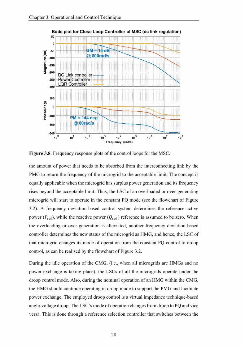
Chapter 3. Operational and Control Technique
28
-300
-250
-200
-150
-100
-50
0
50
100
101
102
103
104
105
106
107
108
-540
-360
-180
0
180
Bode plot for Close Loop Controller of MSC (dc link regulation)
Frequency (rad/s)
Ph
ase
(de
g)
Mag
nit
ud
e(d
b)
PM = 144 deg
@ 80rad/s
GM = 15 dB
@ 800rad/s
DC Link controllerPower ControllerLQR Controller
Figure 3.8. Frequency response plots of the control loops for the MSC.
the amount of power that needs to be absorbed from the interconnecting link by the
PMG to return the frequency of the microgrid to the acceptable limit. The concept is
equally applicable when the microgrid has surplus power generation and its frequency
rises beyond the acceptable limit. Thus, the LSC of an overloaded or over-generating
microgrid will start to operate in the constant PQ mode (see the flowchart of Figure
3.2). A frequency deviation-based control system determines the reference active
power (𝑃ref), while the reactive power (𝑄ref ) reference is assumed to be zero. When
the overloading or over-generation is alleviated, another frequency deviation-based
controller determines the new status of the microgrid as HMG, and hence, the LSC of
that microgrid changes its mode of operation from the constant PQ control to droop
control, as can be realised by the flowchart of Figure 3.2.
During the idle operation of the CMG, (i.e., when all microgrids are HMGs and no
power exchange is taking place), the LSCs of all the microgrids operate under the
droop control mode. Also, during the nominal operation of an HMG within the CMG,
the HMG should continue operating in droop mode to support the PMG and facilitate
power exchange. The employed droop control is a virtual impedance technique-based
angle-voltage droop. The LSC’s mode of operation changes from droop to PQ and vice
versa. This is done through a reference selection controller that switches between the
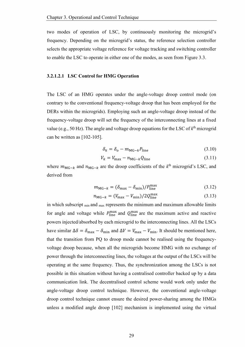
Chapter 3. Operational and Control Technique
29
two modes of operation of LSC, by continuously monitoring the microgrid’s
frequency. Depending on the microgrid’s status, the reference selection controller
selects the appropriate voltage reference for voltage tracking and switching controller
to enable the LSC to operate in either one of the modes, as seen from Figure 3.3.
3.2.1.2.1 LSC Control for HMG Operation
The LSC of an HMG operates under the angle-voltage droop control mode (on
contrary to the conventional frequency-voltage droop that has been employed for the
DERs within the microgrids). Employing such an angle-voltage droop instead of the
frequency-voltage droop will set the frequency of the interconnecting lines at a fixed
value (e.g., 50 Hz). The angle and voltage droop equations for the LSC of kth microgrid
can be written as [102-105].
𝛿𝑘 = 𝛿o − 𝑚MG−𝑘𝑃line (3.10)
𝑉𝑘 = 𝑉max − 𝑛MG−𝑘𝑄line (3.11)
where 𝑚MG−𝑘 and 𝑛MG−𝑘 are the droop coefficients of the kth microgrid’s LSC, and
derived from
𝑚MG−𝑘 = (𝛿max − 𝛿min)/𝑃linemax (3.12)
𝑛MG−𝑘 = (𝑉max − 𝑉min)/2𝑄linemax (3.13)
in which subscript min and max represents the minimum and maximum allowable limits
for angle and voltage while 𝑃linemax and 𝑄line
max are the maximum active and reactive
powers injected/absorbed by each microgrid to the interconnecting lines. All the LSCs
have similar ∆𝛿 = 𝛿max − 𝛿min and ∆𝑉 = 𝑉max − 𝑉min. It should be mentioned here,
that the transition from PQ to droop mode cannot be realised using the frequency-
voltage droop because, when all the microgrids become HMG with no exchange of
power through the interconnecting lines, the voltages at the output of the LSCs will be
operating at the same frequency. Thus, the synchronization among the LSCs is not
possible in this situation without having a centralised controller backed up by a data
communication link. The decentralised control scheme would work only under the
angle-voltage droop control technique. However, the conventional angle-voltage
droop control technique cannot ensure the desired power-sharing among the HMGs
unless a modified angle droop [102] mechanism is implemented using the virtual

Chapter 3. Operational and Control Technique
30
impedance method. To implement the virtual impedance-based modified angle droop,
Equation (3.10) and (3.11) needs to be transformed into the 𝛼𝛽 coordinates and the
voltage across the virtual impedance needs to be subtracted. Hence, the reference angle
and voltage equation can be modified and rewritten 𝛼𝛽 coordinates as
𝑉α−𝑘ref = 𝑉𝑘 cos 𝛿𝑘 + 𝑋v
𝑘𝐼g𝑘 sin 𝜃g
𝑘 (3.14)
𝑉β−𝑘ref = 𝑉𝑘 sin 𝛿𝑘 − 𝑋v
𝑘𝐼g𝑘 cos 𝜃g
𝑘 (3.15)
where 𝑋v𝑘 = 𝜔ref𝐿v
𝑘 and 𝑖g𝑘 = 𝐼g
𝑘∠𝜃g𝑘 are respectively the virtual impedance and
current of the coupling inductance. Then, the reference voltage and phase angle for the
LSC of microgrid-k operating under the modified droop control technique, are
calculated as
𝑉dr𝑘 = √(𝑉α−𝑘
ref )2 + (𝑉β−𝑘ref )2 (3.16)
𝛿dr𝑘 = tan−1 (
𝑉β−𝑘ref
𝑉α−𝑘ref
) (3.17)
From Equation (3.16) and (3.17), the instantaneous reference voltage for the LQR
switching control block of the LSC in microgrid-k can be determined as
𝑉a−𝑘ref = 𝑉dr
𝑘 sin(𝜔ref𝑡 + 𝛿dr𝑘 ) (3.18)
𝑉b−𝑘ref = 𝑉dr
𝑘 sin(𝜔ref𝑡 + 𝛿dr𝑘 − 120°) (3.19)
𝑉c−𝑘ref = 𝑉dr
𝑘 sin(𝜔ref𝑡 + 𝛿dr𝑘 − 240°) (3.20)
where 𝜔ref is selected based on the desired frequency level in the three-phase ac power
lines (e.g., 50 Hz). The virtual impedances to share power between microgrid-i and j
can be calculated based on their droop coefficients as [103, 105-106]
𝑚MG−𝑖
𝑚MG−𝑗=
𝐿g + 𝐿v𝑖
𝐿g + 𝐿v𝑗 (3.21)
Figure 3.9 shows the block diagram of the modified angle-voltage droop control
technique. It may be noted here that, the central controller of a microgrid determines
the amount of power that is going to be shared by each HMG and it is governed by
numerous factors such as distance among the microgrids, cost of power generation,
line loss, willingness to participate in power exchange and so on [106-108]. Different
types of optimization and decision-making techniques are proposed in ref [109-112]
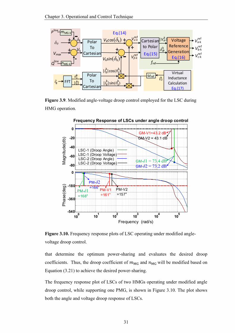
Chapter 3. Operational and Control Technique
31
PolarTo
Cartesian
P
Q
ωref
Cartesian to Polar
Voltage Reference
GenerationEq.(16)
FFT |Ig|
θg
ig
|Vdr|
δdrVmax
δ0 δk
Vk
Vkcos(δk)
fref
mMG-k
Vksin(δk)
+
+
Virtual InductanceCalculation
Eq.(17)
nMG-k
+
+ +
Eq.(14)
Vα-k ref
Vβ-k ref
k
k
k
k
k LVk
Vb-kref
PolarTo
Cartesian
|Ig|cos(θg)k k
|Ig|sin(θg)k k
Va-kref
Vc-kref
line
line
Eq.(15)
Figure 3.9. Modified angle-voltage droop control employed for the LSC during
HMG operation.
-80
-60
-40
-20
0
-540
-360
-180
0
Frequency (rad/s)
101
102
103
104
105
Magn
itu
de(d
b)
Pha
se
(deg
) PM-δ2=166°
PM-δ1=168°
PM-V1
=161°
PM-V2
=157°
GM-V1=43.2 dB
GM-V2 = 43.1 dB
GM-δ1 = 73.4 dBGM-δ2 = 73.2 dB
LSC-1 (Droop Angle)LSC-1 (Droop Voltage)LSC-2 (Droop Angle)LSC-2 (Droop Voltage)
Frequency Response of LSCs under angle droop control
100
Figure 3.10. Frequency response plots of LSC operating under modified angle-
voltage droop control.
that determine the optimum power-sharing and evaluates the desired droop
coefficients. Thus, the droop coefficient of 𝑚MG and 𝑛MG will be modified based on
Equation (3.21) to achieve the desired power-sharing.
The frequency response plot of LSCs of two HMGs operating under modified angle
droop control, while supporting one PMG, is shown in Figure 3.10. The plot shows
both the angle and voltage droop response of LSCs.
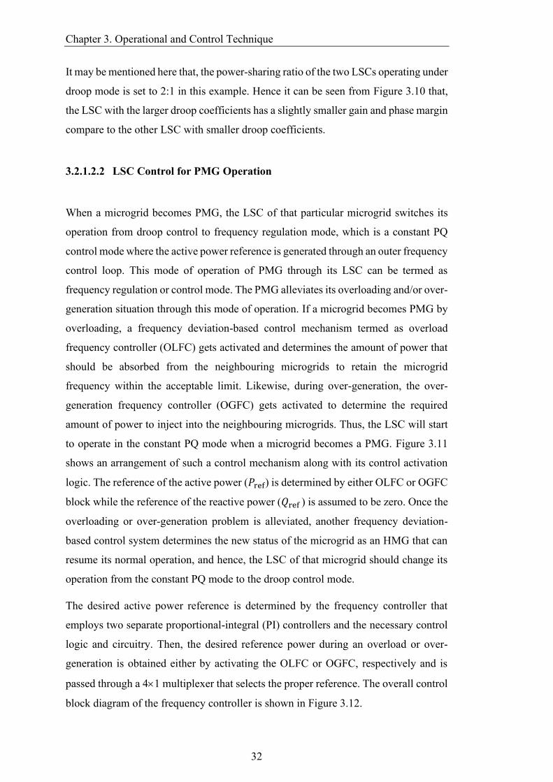
Chapter 3. Operational and Control Technique
32
It may be mentioned here that, the power-sharing ratio of the two LSCs operating under
droop mode is set to 2:1 in this example. Hence it can be seen from Figure 3.10 that,
the LSC with the larger droop coefficients has a slightly smaller gain and phase margin
compare to the other LSC with smaller droop coefficients.
3.2.1.2.2 LSC Control for PMG Operation
When a microgrid becomes PMG, the LSC of that particular microgrid switches its
operation from droop control to frequency regulation mode, which is a constant PQ
control mode where the active power reference is generated through an outer frequency
control loop. This mode of operation of PMG through its LSC can be termed as
frequency regulation or control mode. The PMG alleviates its overloading and/or over-
generation situation through this mode of operation. If a microgrid becomes PMG by
overloading, a frequency deviation-based control mechanism termed as overload
frequency controller (OLFC) gets activated and determines the amount of power that
should be absorbed from the neighbouring microgrids to retain the microgrid
frequency within the acceptable limit. Likewise, during over-generation, the over-
generation frequency controller (OGFC) gets activated to determine the required
amount of power to inject into the neighbouring microgrids. Thus, the LSC will start
to operate in the constant PQ mode when a microgrid becomes a PMG. Figure 3.11
shows an arrangement of such a control mechanism along with its control activation
logic. The reference of the active power (𝑃ref) is determined by either OLFC or OGFC
block while the reference of the reactive power (𝑄ref ) is assumed to be zero. Once the
overloading or over-generation problem is alleviated, another frequency deviation-
based control system determines the new status of the microgrid as an HMG that can
resume its normal operation, and hence, the LSC of that microgrid should change its
operation from the constant PQ mode to the droop control mode.
The desired active power reference is determined by the frequency controller that
employs two separate proportional-integral (PI) controllers and the necessary control
logic and circuitry. Then, the desired reference power during an overload or over-
generation is obtained either by activating the OLFC or OGFC, respectively and is
passed through a 41 multiplexer that selects the proper reference. The overall control
block diagram of the frequency controller is shown in Figure 3.12.
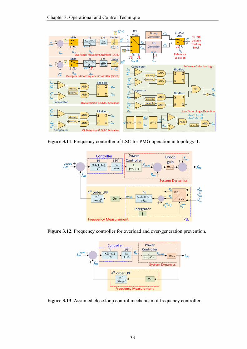
Chapter 3. Operational and Control Technique
33
+
RESET
0 -KOL(1+sTOL)sTOL
QOL
LPF
s+ωOL
ωOL
PI MUX Limiter
fMG
-POLSo
QOL
~ max 0
OLrefP
So
Do
D1
D2
D3
S1
FLrefP =0
+
RESET
0 KOG(1+sTOG)sTOG
QOG
LPF
s+ωOG
ωOG
PI MUX Limiter
fMG
So
QOG
~PmaxOG
0
0
OGrefP
+
+
ANDdelay tc
fMG
ANDdelay tc R
S Q
Q
Flip-Flop
Comparator
OGfLIM
fLIM
OL
OGfFL
fMG
+
+
ANDdelay tc
fMG
ANDdelay tc R
S Q
Q
Flip-FlopOL
fLIM
OLfFL
fMG
QOG
QOG
QOL
QOL
Comparator
OGfLIM
4X1MUX
QOG QOL
DroopController
PQController
RESET
refP
refQ So
Drvc_ref
PQvc_ref3
3
QTr
QTr
refvc
To LQR VoltageTracking
Block
+
+
ANDdelay tr
fMG
ANDdelay tr R
S Q
Q
Flip-FlopOG
fFL
fMG
+
+
ANDdelay tr
fMG
R
S Q
Q
Flip-Flop
OLfFL
fMG
Comparator
OGfFL
QDr
OLfFL
ANDdelay tr
QDr
Comparator
QTr
QTrOR
0
δmin= δ0 - Δδδmax= δ0+Δδ+
+
ANDAND
delay tdr
LPF-1 FFTavg
V line| |
δline δmax
δmin
LPF-2δline
fil
QDr
Reference Selection Logic
OG Detection & OGFC Activation
Overload Frequency Controller (OLFC)
Overgeneration Frequency Controller (OGFC)
3-(2X1)MUX
3
Reference Selection
OL Detection & OLFC Activation
Line Droop Angle Detection
Figure 3.11. Frequency controller of LSC for PMG operation in topology-1.
+ Kf(1+sTf)sTf
LPF
s+ωf
ωf
PI
fMG
fLIM
OL/OG
θg
(sτc +1)1 +
mMG
+fmax
PMG
POL/OG fMG
abc
dqvpcc
a
vpccb
vpccc
KPLL(1+sTPLL)sTPLL
PI 4th order LPF
(s+ωcf)4
ωcf4
2πωMG
+
vd
vq
refv =0q
Integrator
Power Controller
+
System Dynamics
Frequency Measurement
Controller
PLL
Droopgain
MG
+
Figure 3.12. Frequency controller for overload and over-generation prevention.
+ Kf(1+sTf)sTf
LPF
s+ωf
ωf
PI
fMG
fLIM
OL/OG
(sτc +1)1
-mMG
POL/OG fMG
4th order LPF
(s+ωcf)4
ωcf4
Power Controller
+System Dynamics
Controller
Pref
2π
Frequency Measurement
+
Figure 3.13. Assumed close loop control mechanism of frequency controller.

Chapter 3. Operational and Control Technique
34
-500
-400
-300
-200
-100
0
-720
-540
-360
-180
0
100
101
102
103
104
105
106
107 10
8
Frequency (rad/s)
10-1
GM = 20 dB
@ 84.3rad/s
PM = 135 deg
@ 10rad/s
Bode plot for Close Loop Controller of LSC (Freq. Control Mode)
Mag
nit
ud
e(d
b)
Ph
ase(d
eg
)
Frequency controllerPower ControllerLQR Controller
Figure 3.14. Frequency response plots of LSC operating under frequency regulation
mode.
To design the frequency controller, 𝑃MG and 𝑓max can be considered as a disturbance
to the system. The PI controller employed for the PLL is very fast compared to the
overall system dynamics and LPF; hence, the PLL block can be assumed to be a unity
gain block, and thus, the overall control block diagram of Figure 3.12 can be
represented as shown in Figure 3.13. Based on the closed-loop control system of
Figure 3.13, the PI controllers can be designed based on the symmetrical optimum
method as described in [99]. The bode plot of the closed-loop frequency regulation
controller is shown in Figure 3.14.
A proper reference selection logic is required to facilitate a smooth transition between
constant PQ control mode (for FMG and PMG) and droop control mode (for HMG)
without causing unwanted transients, oscillations, and instability. Such an arrangement
to change over between the operating modes of LSC is shown in Figure 3.11. The
three-phase reference voltages are either selected from the droop control block or PQ
controller block through three sets of 21 multiplexers using the reference selection
logic employed in the mode transition controller. Then the appropriate reference
voltages are passed to the LQR voltage tracking and switching control block. When
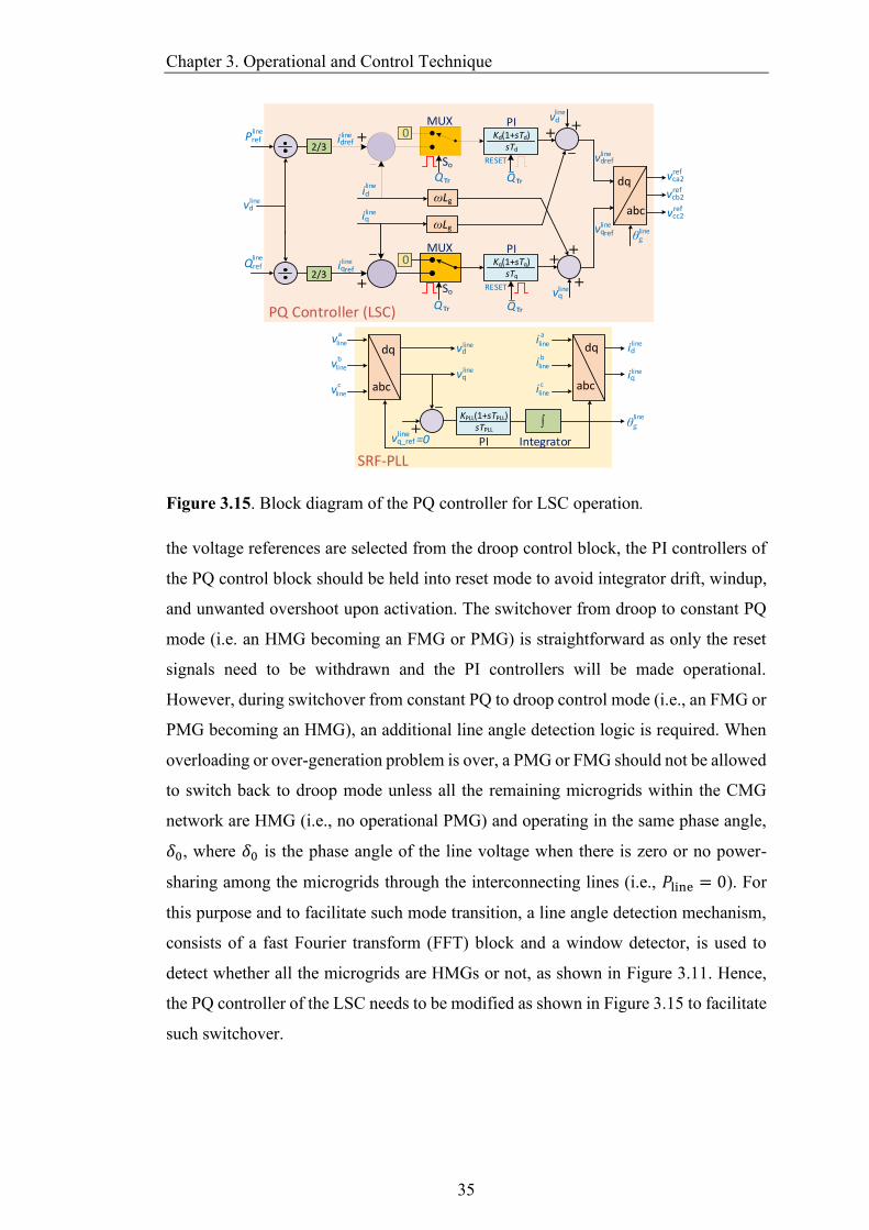
Chapter 3. Operational and Control Technique
35
PQ Controller (LSC)
+
RESET
0 Kd(1+sTd)sTd
QTr
PI MUX
So
QTr
Pref
id
idref
+ RESET
0 Kq(1+sTq)sTq
QTr
PI MUX
So
QTr
Qref
iq
iqref
vd
vd
vq
vdref
vqref
abc
dq
vcc2ref
vcb2ref
vca2ref
++
++
+
θg
ωLg
ωLg
vq
vd
vq_refline
=0
abc
dq dq
abc
id
iq
SRF-PLL
θg
vlinea
vlineb
vlinec
+
KPLL(1+sTPLL)sTPLL
PI Integrator
2/3
2/3
ilinea
ilineb
ilinec
line
line
line
line
line
line
line
line
line
line
line
line
line
line
line
line
line
Figure 3.15. Block diagram of the PQ controller for LSC operation.
the voltage references are selected from the droop control block, the PI controllers of
the PQ control block should be held into reset mode to avoid integrator drift, windup,
and unwanted overshoot upon activation. The switchover from droop to constant PQ
mode (i.e. an HMG becoming an FMG or PMG) is straightforward as only the reset
signals need to be withdrawn and the PI controllers will be made operational.
However, during switchover from constant PQ to droop control mode (i.e., an FMG or
PMG becoming an HMG), an additional line angle detection logic is required. When
overloading or over-generation problem is over, a PMG or FMG should not be allowed
to switch back to droop mode unless all the remaining microgrids within the CMG
network are HMG (i.e., no operational PMG) and operating in the same phase angle,
𝛿0, where 𝛿0 is the phase angle of the line voltage when there is zero or no power-
sharing among the microgrids through the interconnecting lines (i.e., 𝑃line = 0). For
this purpose and to facilitate such mode transition, a line angle detection mechanism,
consists of a fast Fourier transform (FFT) block and a window detector, is used to
detect whether all the microgrids are HMGs or not, as shown in Figure 3.11. Hence,
the PQ controller of the LSC needs to be modified as shown in Figure 3.15 to facilitate
such switchover.
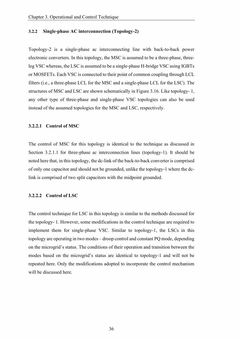
Chapter 3. Operational and Control Technique
36
3.2.2 Single-phase AC interconnection (Topology-2)
Topology-2 is a single-phase ac interconnecting line with back-to-back power
electronic converters. In this topology, the MSC is assumed to be a three-phase, three-
leg VSC whereas, the LSC is assumed to be a single-phase H-bridge VSC using IGBTs
or MOSFETs. Each VSC is connected to their point of common coupling through LCL
filters (i.e., a three-phase LCL for the MSC and a single-phase LCL for the LSC). The
structures of MSC and LSC are shown schematically in Figure 3.16. Like topology- 1,
any other type of three-phase and single-phase VSC topologies can also be used
instead of the assumed topologies for the MSC and LSC, respectively.
3.2.2.1 Control of MSC
The control of MSC for this topology is identical to the technique as discussed in
Section 3.2.1.1 for three-phase ac interconnection lines (topology-1). It should be
noted here that, in this topology, the dc-link of the back-to-back converter is comprised
of only one capacitor and should not be grounded, unlike the topology-1 where the dc-
link is comprised of two split capacitors with the midpoint grounded.
3.2.2.2 Control of LSC
The control technique for LSC in this topology is similar to the methods discussed for
the topology- 1. However, some modifications in the control technique are required to
implement them for single-phase VSC. Similar to topology-1, the LSCs in this
topology are operating in two modes – droop control and constant PQ mode, depending
on the microgrid’s status. The conditions of their operation and transition between the
modes based on the microgrid’s status are identical to topology-1 and will not be
repeated here. Only the modifications adopted to incorporate the control mechanism
will be discussed here.

Chapter 3. Operational and Control Technique
37
Rg Lg Rf Lf
Cdc
MG
MSC
Cf
dc Link
LCLFilter
vg
igabc
ifabc
vcabc
abc
Vdc
(Vdc )ref 2
Compensator PQ Controller
Pref
Qref
refvc
vg
(.)2
(PLL)
vq vd
θg
iq id
ig
Power Controldc Voltage Control
+
3
3
Voltage Tracking
dq
abc abc
dq
3
if
vc
3LQR
switchingcontroller
Gate Pulses
6
+
Vdc
Rf Lf Rg Lg
Cf
if
vc
ig
LSC
vg
1- ph Power exchange link
Voltage Tracking
if
vc
LQRswitchingcontroller
Gate Pulses
4
1
1abc
abc
Reference Selection
Logic
fMG
vg1
fFL
fFL
PIPQ Controller Pref
Qref
(PLL)vqvd
θg
iqid
Frequency Control
Reset
dqαβ
dq
refvc
ReferenceVoltage
Generation Q
|Vdr|
δdr
Droop Controller
Power Calculation
Pvg
ig
vg
ig
fLIMOG fLIM
OL
fFLOG
fFLOL
fMG
Droop Control
abc
abc
1
3
OG
OL
αβ
1
1
vc_drref
vc_PQref
MUX+1
-90°
-90°
TM1TM2TM3 TL1 TL2
BL1 BL2BM1BM2BM3
line
line
line
line
MG
lineline line line
line
Figure 3.16. Assumed structure and close loop control mechanism of the MSC and
LSC for topology-2.
+
+ R
S Q
Q
Flip-Flop+
vc
if
k1
k2
k3
+-h
+h
upos
TL1
BL1
+
+ R
S Q
Q
Flip-Flop-k1
-k2
-k3
+-h
+hTL2
BL1
if~
vcref
uneg
s+ωc
s
LQR Switching Controller-1ph
Figure 3.17. Linear Quadratic Regulator based switching and voltage tracking for
single-phase VSC.
The first key difference is reference voltage generation for the single-phase VSC while
operating in droop mode (i.e., HMG operation). In this regard, based on Equation
(3.16) and (3.17), the instantaneous reference voltage for single-phase VSC can be
expressed as
𝑉a−𝑘ref = 𝑉dr
𝑘 sin(𝜔ref𝑡 + 𝛿dr𝑘 ) (3.22)
𝑉b−𝑘ref = 𝑉dr
𝑘 sin(𝜔ref𝑡 + 𝛿dr𝑘 − 180°) (3.23)
which are the reference voltages, 𝑣cref for the single-phase LSC and applied to the LQR
voltage tracking and switching block. Thus, the LQR switching controller needs to be
Chapter 3. Operational and Control Technique
38
-80
-60
-40
-20
0
20
-360
-270
-180
-90
0
Frequency Response of 1-ph LSC under angle droop control
Frequency (rad/s)
101
102
103
104
105
100
Magn
itu
de(d
b)
Pha
se(d
eg
)
GM-δ = 83dB
GM-V = 62 dB
PM-V=70°
PM-δ =165°
LSC-1ph (Droop Angle)
LSC-1ph (Droop Voltage)
Figure 3.18. Frequency response of single-phase LSC operating under modified
angle-voltage droop control.
PQ Controller (LSC-1ph)
+
RESET
0 Kd(1+sTd)sTd
QTr
PI MUX
So
QTr
Pref
id
idref
+ RESET
0 Kq(1+sTq)sTq
QTr
PI MUX
So
QTr
Qref
iq
iqref
vd
vd
vq
vdref
vqref
αβ
dq vcref
++
++
+
θg
ωLg
ωLg
αβ
dq dq
id
iq
SRF-PLL (1ph)
θg+
KPLL(1+sTPLL)sTPLL
PI Integrator
2
2
(vα)
(vβ)
αβ
line
lineline
line
line
line
line
line
line
line
line
line
line
vg
2nd order LPF
(s+ωps)2
ωps2
2
(vα)
(vβ)
vq_refline
=0
vdline
90° Phase Shift
vqline
ig
2nd order LPF
(s+ωps)2
ωps2
2
90° Phase Shift
(iα)
(iβ) line
line
Figure 3.19. Block diagram of the PQ controller for single-phase LSC.
modified as shown in Figure 3.17. The bode plots for single-phase LSC operating
under droop control are shown in Figure 3.18. It can be observed from Figure 3.18

Chapter 3. Operational and Control Technique
39
that, the single-phase LSC has a relatively smaller phase and gain margin as compared
to the three-phase LSC. In other words, the three-phase LSC operating in droop mode
appears to be more stable than the single-phase LSC.
Finally, the PQ controller for the LSC needs to be modified and implemented for
single-phase topology. The single-phase PQ controller implemented in dq frame for
LSC is shown in Figure 3.19 along with its reset and control signals. To implement the
PQ controller in dq frame for a single-phase converter, 𝛼𝛽 to dq transformation (Clark
transformation) is used where the measured line voltage 𝑣g and current 𝑖g are the 𝛼
components for voltage and current respectively, whereas a 90° phase-shifted version
of 𝑣g and 𝑖g are the 𝛽 components for voltage and current. The phase shift in voltage
and current are introduced by a critically damped second order low pass filter that
operates with a gain of 0.5 and phase shift of 90° at its cross over frequency, 𝜔ps
(which is 50Hz or 314.16rad/s in this case). To compensate for this gain of 0.5, the
signal needs to be amplified with a gain of 2. To determine the angle of the
interconnection line, 𝜃gline , a synchronous reference frame PLL is used as before.
3.2.3 DC interconnection (Topology-3)
Topology-3 is a dc interconnecting line with a single VSC. It is connected to the
microgrid’s three-phase ac lines and facilitates bi-directional power flow between the
microgrid and the dc-link. The dc-links are directly connected to the dc interconnecting
lines that form the CMG network. In this topology, a single VSC serves the functions
of both the MSC and LSC of the previous two topologies. The VSC connected to each
HMG within the CMG regulates the dc voltage across the dc-link capacitor. As the
HMGs will share the power injected/absorbed by the PMGs of the CMG, an active
power-dc voltage droop technique is employed that determines the reference dc
voltage such that the power shared by the HMGs is as defined by the ratios of the droop
coefficients. On the other hand, the VSC connected to each PMG operates in constant
PQ mode and facilitates absorption or injection of the required active power to retain
and regulate the frequency of the PMG within its acceptable limits. The structure and
control mechanism of the VSC are discussed in the following subsections:
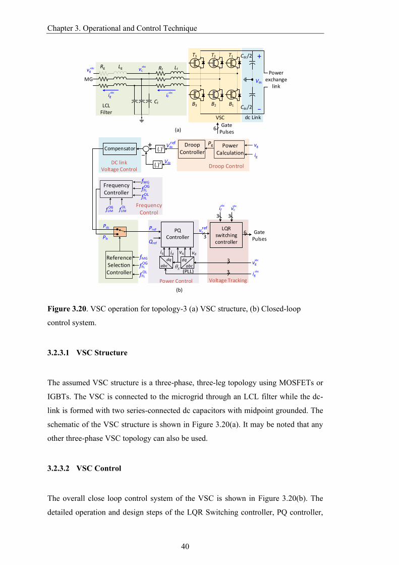
Chapter 3. Operational and Control Technique
40
Rg Lg Rf Lf
Cdc/2
MG
VSC
Cf
dc Link
LCLFilter
vg
igabc
ifabc
vcabc
abc
Vdc
Gate Pulses
+
Power exchange
link
6(a)
Compensator
PQ Controller
Pref
Qref
refvc
vg
(PLL)
vq vd
θg
iq id
igPower Control
+
3
Voltage Tracking
dq
abc abc
dq
3
if vc
3
LQRswitchingcontroller
abcabc
Frequency Controller
Droop Controller
Power Calculation
Pg vg
ig
fLIMOG fLIM
OL
fFLOG
fFLOL
fMG
Droop Control
abc
abc
3
(.)2 Vdc ref
(.)2 Vdc
Frequency Control
Reference Selection Controller
fMG
fFL
fFL
OG
OL
DC link Voltage Control
6 Gate Pulses
(b)
Pdc
Pfr
3
Cdc/2
T1T2T3
B1B2B3
Figure 3.20. VSC operation for topology-3 (a) VSC structure, (b) Closed-loop
control system.
3.2.3.1 VSC Structure
The assumed VSC structure is a three-phase, three-leg topology using MOSFETs or
IGBTs. The VSC is connected to the microgrid through an LCL filter while the dc-
link is formed with two series-connected dc capacitors with midpoint grounded. The
schematic of the VSC structure is shown in Figure 3.20(a). It may be noted that any
other three-phase VSC topology can also be used.
3.2.3.2 VSC Control
The overall close loop control system of the VSC is shown in Figure 3.20(b). The
detailed operation and design steps of the LQR Switching controller, PQ controller,
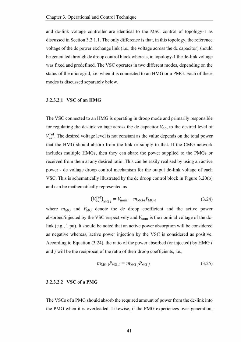
Chapter 3. Operational and Control Technique
41
and dc-link voltage controller are identical to the MSC control of topology-1 as
discussed in Section 3.2.1.1. The only difference is that, in this topology, the reference
voltage of the dc power exchange link (i.e., the voltage across the dc capacitor) should
be generated through dc droop control block whereas, in topology-1 the dc-link voltage
was fixed and predefined. The VSC operates in two different modes, depending on the
status of the microgrid, i.e. when it is connected to an HMG or a PMG. Each of these
modes is discussed separately below.
3.2.3.2.1 VSC of an HMG
The VSC connected to an HMG is operating in droop mode and primarily responsible
for regulating the dc-link voltage across the dc capacitor 𝑉dc, to the desired level of
𝑉dcref. The desired voltage level is not constant as the value depends on the total power
that the HMG should absorb from the link or supply to that. If the CMG network
includes multiple HMGs, then they can share the power supplied to the PMGs or
received from them at any desired ratio. This can be easily realised by using an active
power - dc voltage droop control mechanism for the output dc-link voltage of each
VSC. This is schematically illustrated by the dc droop control block in Figure 3.20(b)
and can be mathematically represented as
(𝑉dcref)
MG-𝑖= 𝑉nom − 𝑚MG-𝑖𝑃MG-𝑖 (3.24)
where 𝑚MG and 𝑃MG denote the dc droop coefficient and the active power
absorbed/injected by the VSC respectively and 𝑉nom is the nominal voltage of the dc-
link (e.g., 1 pu). It should be noted that an active power absorption will be considered
as negative whereas, active power injection by the VSC is considered as positive.
According to Equation (3.24), the ratio of the power absorbed (or injected) by HMG 𝑖
and 𝑗 will be the reciprocal of the ratio of their droop coefficients, i.e.,
𝑚MG-𝑖𝑃MG-𝑖 = 𝑚MG-𝑗𝑃MG-𝑗 (3.25)
3.2.3.2.2 VSC of a PMG
The VSCs of a PMG should absorb the required amount of power from the dc-link into
the PMG when it is overloaded. Likewise, if the PMG experiences over-generation,
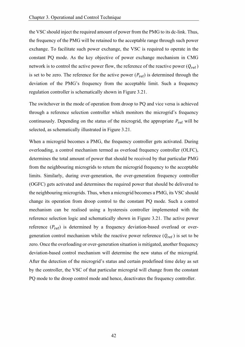
Chapter 3. Operational and Control Technique
42
the VSC should inject the required amount of power from the PMG to its dc-link. Thus,
the frequency of the PMG will be retained to the acceptable range through such power
exchange. To facilitate such power exchange, the VSC is required to operate in the
constant PQ mode. As the key objective of power exchange mechanism in CMG
network is to control the active power flow, the reference of the reactive power (𝑄ref )
is set to be zero. The reference for the active power (𝑃ref) is determined through the
deviation of the PMG’s frequency from the acceptable limit. Such a frequency
regulation controller is schematically shown in Figure 3.21.
The switchover in the mode of operation from droop to PQ and vice versa is achieved
through a reference selection controller which monitors the microgrid’s frequency
continuously. Depending on the status of the microgrid, the appropriate 𝑃ref will be
selected, as schematically illustrated in Figure 3.21.
When a microgrid becomes a PMG, the frequency controller gets activated. During
overloading, a control mechanism termed as overload frequency controller (OLFC),
determines the total amount of power that should be received by that particular PMG
from the neighbouring microgrids to return the microgrid frequency to the acceptable
limits. Similarly, during over-generation, the over-generation frequency controller
(OGFC) gets activated and determines the required power that should be delivered to
the neighbouring microgrids. Thus, when a microgrid becomes a PMG, its VSC should
change its operation from droop control to the constant PQ mode. Such a control
mechanism can be realised using a hysteresis controller implemented with the
reference selection logic and schematically shown in Figure 3.21. The active power
reference (𝑃ref) is determined by a frequency deviation-based overload or over-
generation control mechanism while the reactive power reference (𝑄ref ) is set to be
zero. Once the overloading or over-generation situation is mitigated, another frequency
deviation-based control mechanism will determine the new status of the microgrid.
After the detection of the microgrid’s status and certain predefined time delay as set
by the controller, the VSC of that particular microgrid will change from the constant
PQ mode to the droop control mode and hence, deactivates the frequency controller.
Chapter 3. Operational and Control Technique
43
refvc
+
RESET
0 KOL(1+sTOL)sTOL
QOL
LPF
s+ωOL
ωOL
PI MUX Limiter
fMG
-POLSo
QOL
~ max 0
OLrefP
So
Do
D1
D2
D3
S1
FLrefP =0
+
RESET
0 -KOG(1+sTOG)sTOG
QOG
LPF
s+ωOG
ωOG
PI MUX Limiter
fMG
So
QOG
~PmaxOG
0
0
OGrefP
+
+
ANDdelay tc
fMG
ANDdelay tc R
S Q
Q
Flip-Flop
Comparator
OGfLIM
fLIM
OL
OGfFL
fMG
+
+
ANDdelay tc
fMG
ANDdelay tc R
S Q
Q
Flip-FlopOL
fLIM
OLfFL
fMG
QOG
QOG
QOL
QOL
Comparator
OGfLIM
4X1MUX
QOG QOL
PQController
refP
refQSo
QTr
To LQR VoltageTracking
Block
0
OG Detection & OGFC Activation
Overload Frequency Controller (OLFC)
Overgeneration Frequency Controller (OGFC)
Reference Selection
OL Detection & OLFC Activation
Compensator
DC Link Voltage Control
+(.)2Vdc
ref
(.)2
Kdc(s+ωz)s(s+ωp)
0 MUX
SoPg
frP
Pdc
+Vdc
rated
+
+
ANDdelay tr
fMG
ANDdelay tr R
S Q
Q
Flip-FlopOG
fFL
fMG
+
+
ANDdelay tr
fMG
R
S Q
Q
Flip-Flop
OLfFL
fMG
Comparator
OGfFL
OLfFL
ANDdelay tr
Comparator QTr
QTrOR
Reference Selection Logic
mMG-k Vdc
Droop ControlQTr
3
Figure 3.21. Frequency regulation controller of VSC for PMG operation in
topology- 3.
The frequency controller determines the desired power reference through two different
PI-based closed-loop control systems along with its necessary control logic and
circuitry. Then, the desired power reference is selected through a 41 Multiplexer
circuit that selects the proper power reference during the overload or excess-generation
situation respectively by activating the OLFC or OGFC. To coordinate between droop
control mode (for HMG) and constant PQ control mode (for the FMG and PMG), a
proper reference selection logic is needed to switch over between the modes smoothly
without causing unwanted transients, oscillations, and instability. The reference
selector will select proper active power reference either from the droop control-based
dc-link controller block or frequency controller block through a 21 multiplexer and
pass it to the PQ control block. Once a PMG becomes an HMG, the reference selector
will enable the VSC to switch back to droop-based dc-link voltage control mode.

Chapter 3. Operational and Control Technique
44
3.3 Coordinated Power Sharing among BES and CMG
This study proposes a two-stage, coordinated power-sharing strategy among BES and
coupled microgrids for overload management in autonomous microgrids, through
dynamic frequency control. Both local BES and the neighbouring microgrids can work
in conjunction or individually to supply the required overload power demand. For this,
BES’ state of charge should be above a minimum level and extra power generation
capacity needs to be available in the neighbouring microgrids. A predefined
framework with appropriate constraints and conditions, under which the power
exchange will take place, is defined and formulated. For this purpose, two different
self-healing agents, functioning in a decentralised (communication free) manner. This
is realised by continuously monitoring the microgrid frequency and its BES unit’s
SoC. This information is then used to cooperatively activate or deactivate two
developed self-healing agents, namely, battery frequency controller (BFC) for BES
unit, and interconnection frequency controller (IFC) for the coupling of microgrids.
These self-healing agents dynamically modify the amount of internal and external
power exchange levels based on the BES units’ SoC and the microgrids’ loading
condition.
3.3.1 Network Structure
Let us consider a system of Figure 3.22 where N autonomous microgrids, each
consisting of multiple DERs, DGs, loads, one BES and one inter-connection converter
(ICC). Each microgrid is monitored, supervised, and controlled through its microgrid
central controller, termed as MGCC. The DERs and BES are connected to the
microgrid through VSCs. Different VSCs are controlled in different operating modes
to regulate the power and frequency of each microgrid. The VSCs of DERs are
assumed to be operating in the 𝑃 − 𝑓 and 𝑄 − 𝑉 droop control mode [73]. It is assumed
that each DER is provided with its local energy storage and thus they can be
represented as a dispatchable DER. The structure and operation of the DERs are
discussed in [11-12, 73] and is not repeated here. It should be noted that these local
storages are independent and different from the BES of each microgrid as the BESs
are assigned to support the microgrids in the event of power deficiency and
Chapter 3. Operational and Control Technique
45
BES
Load
DER
VSCVSC
BSC
DG
BES
Load
DER
VSCVSC
BSC
DG
BES Load
DER
VSCVSC
BSCDG
ICCICC
PowerExchange
Link
MG-1
MG-2
MG-3BESLoad
DER
VSCVSC
BSCDG
ICC
MG-N
Large Remote
Area
ICC
Figure 3.22. Autonomous CMG network with BES to coordinate power-sharing
dynamically regulate the frequency within the acceptable limit. The BES is connected
to the microgrid through a separate VSC termed as Battery Energy Storage converter
(BSC) that operates in constant PQ mode. The charging or discharging mode of the
BES is determined by the MGCC, based on the MG’s loading condition. Finally, each
microgrid is connected to a common dc power exchange link through its ICC to
exchange power with the other microgrids in the event of overloading or power
deficiency. Each microgrid can operate independently at any predefined voltage and
frequency level without affecting the operation of other neighbouring microgrids.
3.3.2 Control of Converters
The structure of the BSC and ICC are assumed identical and their overall control block
diagram is shown in Figure 3.23. Both BSC and ICC are VSCs connected to their
respective MG, which enable bi-directional power flow with BES and the dc power
exchange link, respectively. Each converter is working in constant PQ mode and has
three cascaded feedback control loops, namely, voltage tracking, power control and
reference power generation loop, as can be seen from Figure 3.23. The voltage tracking
and power control loop are identical for both converters, whereas, the reference power
generation loop, which is the most outer loop, is different and depends on the mode of
operation of the microgrid and converter.

Chapter 3. Operational and Control Technique
46
Rg Lg Rf Lf
Cdc
MG(PCC)
BSC/ICC
Cf
DC Link
LCL Filter
vpcc
igabc
ifabc
vcabcabc
Vdc
DC link Controller
PQ Controller
Pref
Qref
refvc
vpcc
(PLL)
vq vd
θg
iq id
ig
Power ControlRef. Power Generation
3
3
Voltage Tracking
dqabc abc
dq
3
if
vc
3LQR
switchingcontroller
Gate Pulses
6
+
abc
abc
abc
abc
3
or Vbatt
+
BES
T1T2T3
B1B2B3
BFC
BES Controller
Vdc
ref
Vdc
fMG
fmin
Pref
BSC
SoCbatt
Vbatt
IFC
Figure 3.23. Assumed structure and closed-loop control block diagram of VSC and
filter system for BSC/ICC
3.3.2.1 Converters Structure
The BSC and ICC structure is assumed to be a three-phase, three-leg VSC using IGBTs
or MOSFETs, as schematically shown in Figure 3.23. They are connected to the
microgrid through an LCL filter to effectively filter out the undesired switching
harmonics. The dc side of the BSC is connected to the BES while a dc capacitor is
installed on the dc-link side of the ICC to interconnect it to the power exchange link.
It is to be noted that, any other three-phase VSC topology can also be used for BSC
and ICC.
3.3.2.2 Converter Control Technique
Both converters are operating in constant PQ mode irrespective of the loading
condition of the MG. Only the respective VSC’s output power reference varies
depending on the MG’s loading condition and the outermost control loop which is
active during that time. The BSC is primarily controlled by the MGCC through the
BES controller block, operating as the outermost loop. The BFC gets activated and
operates in conjunction with the BES controller during an overloading situation. On
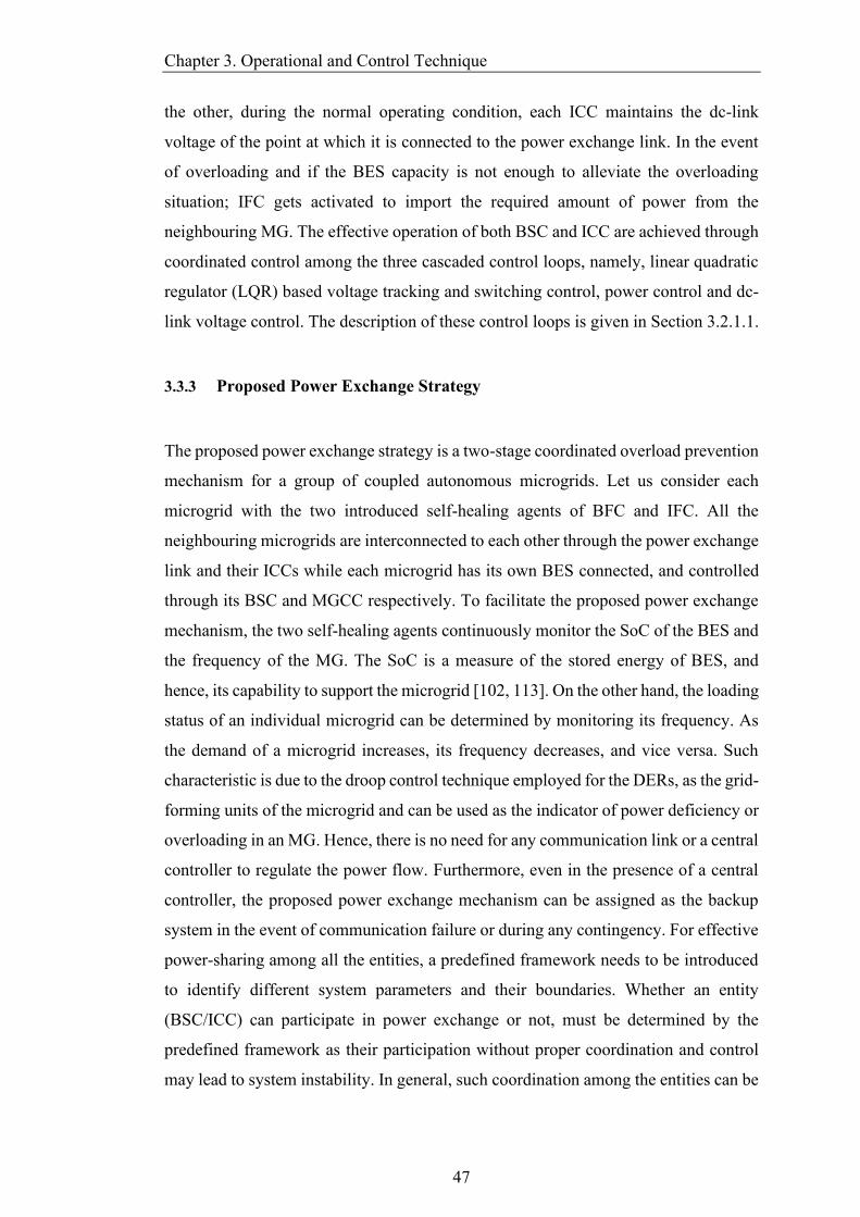
Chapter 3. Operational and Control Technique
47
the other, during the normal operating condition, each ICC maintains the dc-link
voltage of the point at which it is connected to the power exchange link. In the event
of overloading and if the BES capacity is not enough to alleviate the overloading
situation; IFC gets activated to import the required amount of power from the
neighbouring MG. The effective operation of both BSC and ICC are achieved through
coordinated control among the three cascaded control loops, namely, linear quadratic
regulator (LQR) based voltage tracking and switching control, power control and dc-
link voltage control. The description of these control loops is given in Section 3.2.1.1.
3.3.3 Proposed Power Exchange Strategy
The proposed power exchange strategy is a two-stage coordinated overload prevention
mechanism for a group of coupled autonomous microgrids. Let us consider each
microgrid with the two introduced self-healing agents of BFC and IFC. All the
neighbouring microgrids are interconnected to each other through the power exchange
link and their ICCs while each microgrid has its own BES connected, and controlled
through its BSC and MGCC respectively. To facilitate the proposed power exchange
mechanism, the two self-healing agents continuously monitor the SoC of the BES and
the frequency of the MG. The SoC is a measure of the stored energy of BES, and
hence, its capability to support the microgrid [102, 113]. On the other hand, the loading
status of an individual microgrid can be determined by monitoring its frequency. As
the demand of a microgrid increases, its frequency decreases, and vice versa. Such
characteristic is due to the droop control technique employed for the DERs, as the grid-
forming units of the microgrid and can be used as the indicator of power deficiency or
overloading in an MG. Hence, there is no need for any communication link or a central
controller to regulate the power flow. Furthermore, even in the presence of a central
controller, the proposed power exchange mechanism can be assigned as the backup
system in the event of communication failure or during any contingency. For effective
power-sharing among all the entities, a predefined framework needs to be introduced
to identify different system parameters and their boundaries. Whether an entity
(BSC/ICC) can participate in power exchange or not, must be determined by the
predefined framework as their participation without proper coordination and control
may lead to system instability. In general, such coordination among the entities can be
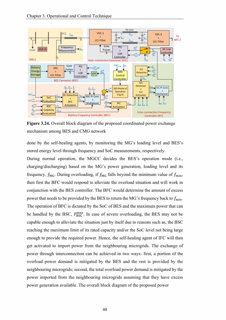
Chapter 3. Operational and Control Technique
48
DER-NLoad
BatteryEnergyStorage
PCC
FrequencyMeasurement
VSC+
LCL Filter
+
LPF
BSC Capacity
Evaluation
PQ+
LQRController
OL Detection+
BFC Activation
BSC PI Cont.+
Multiplexer
fMG frcfmin
SoCbatt
SoCminQBSC
QCAP
QSoC
QSoC
SoC Evaluation
BSCPmax
BES Mode of Operation
(Fig.4)
+
Q =0BSC
ref
PQ+
LQRController
QIFC
Qdct
PICC
dct
PICC
dct
-PICC
ICC PI Cont.+
MultiplexerQBSC
QICC
QICC
PICC
Pdc
VSC-1+
LCL Filter
VSC-2+
LCL Filter
QICC Vdc Vdcref
To MG-2
MG-1
6
6
GatePulses
GatePulses
Q =0ICC
ref
3Inter-connection Converter (ICC)
Battery Frequency Controller (BFC)
33
Pref
BSC
Inter-connection FrequencyController (IFC)
BES Converter (BSC)
DC LinkController
PICC
ref
+Vdc1
Zline
ZlineZMG
Tie-Line
MG Central
Controller
3
IFCActivation
ICCDetection
O/L Detection
+ICC
Activation
SoCbattfMG
+Vdc2
ICC
OL
So
Pbatt
ref
PBSC
OL
BSCP
BSCP rcQCAP
QSoC
QSoC
fMG fmin
fMG frcfminfMG fmin
fMG
Figure 3.24. Overall block diagram of the proposed coordinated power exchange
mechanism among BES and CMG network
done by the self-healing agents, by monitoring the MG’s loading level and BES’s
stored energy level through frequency and SoC measurements, respectively.
During normal operation, the MGCC decides the BES’s operation mode (i.e.,
charging/discharging) based on the MG’s power generation, loading level and its
frequency, 𝑓MG. During overloading, if 𝑓MG falls beyond the minimum value of 𝑓min,
then first the BFC would respond to alleviate the overload situation and will work in
conjunction with the BES controller. The BFC would determine the amount of excess
power that needs to be provided by the BES to return the MG’s frequency back to 𝑓min.
The operation of BFC is dictated by the SoC of BES and the maximum power that can
be handled by the BSC, 𝑃BSCmax. In case of severe overloading, the BES may not be
capable enough to alleviate the situation just by itself due to reasons such as, the BSC
reaching the maximum limit of its rated capacity and/or the SoC level not being large
enough to provide the required power. Hence, the self-healing agent of IFC will then
get activated to import power from the neighbouring microgrids. The exchange of
power through interconnection can be achieved in two ways- first, a portion of the
overload power demand is mitigated by the BES and the rest is provided by the
neighbouring microgrids; second, the total overload power demand is mitigated by the
power imported from the neighbouring microgrids assuming that they have excess
power generation available. The overall block diagram of the proposed power
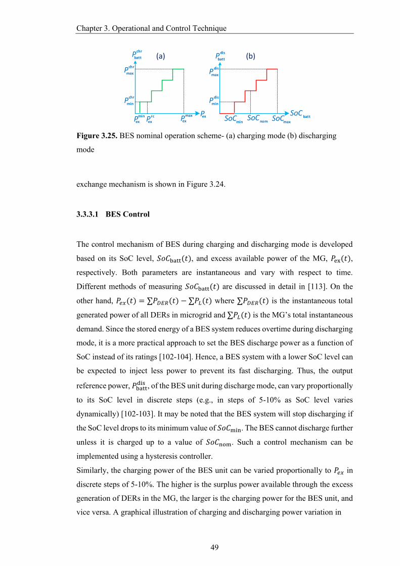
Chapter 3. Operational and Control Technique
49
Pbatt
chr
Pbatt
dis
PexPex
minPex
rc
Pmax
chr
Pmin
chr
Pex
max SoCbattSoC
nomSoCmin
Pmax
dis
Pmin
dis
SoCmax
(a) (b)
Figure 3.25. BES nominal operation scheme- (a) charging mode (b) discharging
mode
exchange mechanism is shown in Figure 3.24.
3.3.3.1 BES Control
The control mechanism of BES during charging and discharging mode is developed
based on its SoC level, 𝑆𝑜𝐶batt(𝑡), and excess available power of the MG, 𝑃ex(𝑡),
respectively. Both parameters are instantaneous and vary with respect to time.
Different methods of measuring 𝑆𝑜𝐶batt(𝑡) are discussed in detail in [113]. On the
other hand, 𝑃𝑒𝑥(𝑡) = ∑𝑃𝐷𝐸𝑅(𝑡) − ∑𝑃𝐿(𝑡) where ∑𝑃𝐷𝐸𝑅(𝑡) is the instantaneous total
generated power of all DERs in microgrid and ∑𝑃𝐿(𝑡) is the MG’s total instantaneous
demand. Since the stored energy of a BES system reduces overtime during discharging
mode, it is a more practical approach to set the BES discharge power as a function of
SoC instead of its ratings [102-104]. Hence, a BES system with a lower SoC level can
be expected to inject less power to prevent its fast discharging. Thus, the output
reference power, 𝑃battdis , of the BES unit during discharge mode, can vary proportionally
to its SoC level in discrete steps (e.g., in steps of 5-10% as SoC level varies
dynamically) [102-103]. It may be noted that the BES system will stop discharging if
the SoC level drops to its minimum value of 𝑆𝑜𝐶min. The BES cannot discharge further
unless it is charged up to a value of 𝑆𝑜𝐶nom. Such a control mechanism can be
implemented using a hysteresis controller.
Similarly, the charging power of the BES unit can be varied proportionally to 𝑃𝑒𝑥 in
discrete steps of 5-10%. The higher is the surplus power available through the excess
generation of DERs in the MG, the larger is the charging power for the BES unit, and
vice versa. A graphical illustration of charging and discharging power variation in
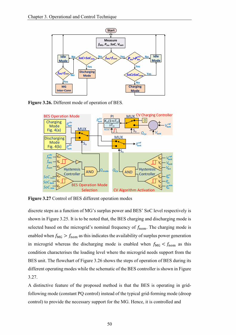
Chapter 3. Operational and Control Technique
50
Yes
Start
Measure fMG, Pex, SoC, Vbatt
fMG>fnomNo
Pex>Pexmin No
Yes
IdleMode
SoC SoCmaxYes
No
SoC>SoCmin
DischargingMode
Yes
IdleMode
fMG<fmin
No
Yes
No
MGInter-Conn
ChargingMode
Figure 3.26. Different mode of operation of BES.
VUT
Vin
VLT
Vbattref
AND
So
0+
VUT
Vin
VLT VLT
Vin
VUT
VLT
Vin
VUT
AND
So
So
RESET
Vbatt
Vdct
Vbattref
VbattQCV
Pbattref
Pbatt
chr
Pbatt
dis
PbattCV
Kcv(1+sTcv)sTcv
QmodeHysteresisController
HysteresisController
Pexmin
Pex
Pexrc
fMG
fMGchr
fnom
SoC min
nomSoC
BES Operation Mode Selection CV Algorithm Activation
CV Charging ControllerBES Operation Mode
MUX
PI MUX
MUX
SoC batt
ChargingMode
Fig. 4(a)
DischargingMode
Fig. 4(b)
QCV
Figure 3.27 Control of BES different operation modes
discrete steps as a function of MG’s surplus power and BES’ SoC level respectively is
shown in Figure 3.25. It is to be noted that, the BES charging and discharging mode is
selected based on the microgrid’s nominal frequency of 𝑓nom. The charging mode is
enabled when 𝑓MG > 𝑓nom as this indicates the availability of surplus power generation
in microgrid whereas the discharging mode is enabled when 𝑓MG < 𝑓nom as this
condition characterises the loading level where the microgrid needs support from the
BES unit. The flowchart of Figure 3.26 shows the steps of operation of BES during its
different operating modes while the schematic of the BES controller is shown in Figure
3.27.
A distinctive feature of the proposed method is that the BES is operating in grid-
following mode (constant PQ control) instead of the typical grid-forming mode (droop
control) to provide the necessary support for the MG. Hence, it is controlled and

Chapter 3. Operational and Control Technique
51
Start
Measure fMG, PBSC, SoC
fMG<fnom
SoC>SoCmin
ActivateBFC
QICC=0 ?
BES Nominal Operation
BSC (PQ mode) ICC (DC Link)
Yes
No
No
Yes
PBSC PBSCmax Deactivate
BFC
BES Nom. Op +
OverloadMitigation
BSC (PQ mode) ICC (DC Link)
OverloadPower
Generation
ICC (DC Link)BSC (PQ mode)
Load-shedding
ActivateIFC
ICC (PQ mode)BSC (PQ mode)
Import
BES Nom. Op
Overload Power+
Yes
No
Yes No
Figure 3.28. Proposed overload management scheme and its different modes of
operation
monitored through the MGCC. This proposed mechanism offers better control and
more flexibility in power-sharing via BES units. Also, the stability issues associated
with droop control are eliminated; as in the droop control technique, it is important to
select the proper droop coefficients to ensure system stability [102]. Most of the
commercially available batteries are needed to be charged in constant current-constant
voltage mode for optimum performance and longer lifecycle, also known as healthy
charging [114]. Such a CC-CV charging approach is not realizable in the droop control
technique. But with the proposed BES control mechanism, constant-voltage healthy
charging mode can be easily implemented as shown in Figure 3.27.
3.3.3.2 Operation of BFC and BSC
The BFC is the outermost control loop that gets activated and operates in conjunction
with the BES controller and regulates the output power of BSC during overload
situation. To better understand the operation of BFC and BSC, let us consider the
flowchart of Figure 3.28. During the nominal operating condition of the MG, the BSC
will receive the power reference from the BES controller and the charging/discharging
mode will be decided based on the developed logic. The BFC will only get activated
during discharge mode when there is no surplus power generation available in MG.
Thus, the activation and operation of BFC is governed by 𝑓MG, 𝑆𝑜𝐶batt and 𝑃BSCmax. The
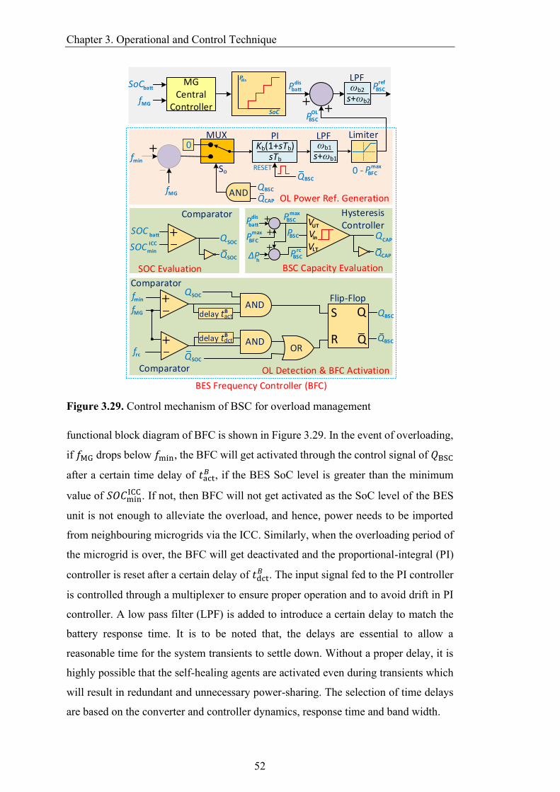
Chapter 3. Operational and Control Technique
52
+
RESET
0
AND
Kb(1+sTb)sTb
QBSC
QBSC
QCAP
LPF
s+ωb1
ωb1
PI MUX Limiter
0 -
P
SoC
MG Central
Controller
SoCbatt
fMG ++
LPF
s+ωb2
ωb2
fMG
fmin
+SOC batt
SOCmin
QCAP
SOC Evaluation
PBSCref
VUT
Vin
VLT
PBSCmax
PBSC
PBSCrc
BSC Capacity Evaluation
+
Pbattdis
PBSC
Comparator HysteresisController
QSOCQCAP
QSOC
+
ANDdelay tact
B
fmin
fMG
ANDdelay tdctB
frcOR
QSOC
QSOC
R
S Q
Q
QBSC
QBSC
Flip-Flop
Comparator
Comparator
OL Detection & BFC Activation
OL
OL Power Ref. Generation
Pbatt
dis
PBFCmax
PBFC
max
ΔP h
+
+
+ICC
dis
So
BES Frequency Controller (BFC)
Figure 3.29. Control mechanism of BSC for overload management
functional block diagram of BFC is shown in Figure 3.29. In the event of overloading,
if 𝑓MG drops below 𝑓min, the BFC will get activated through the control signal of 𝑄BSC
after a certain time delay of 𝑡act𝐵 , if the BES SoC level is greater than the minimum
value of 𝑆𝑂𝐶minICC . If not, then BFC will not get activated as the SoC level of the BES
unit is not enough to alleviate the overload, and hence, power needs to be imported
from neighbouring microgrids via the ICC. Similarly, when the overloading period of
the microgrid is over, the BFC will get deactivated and the proportional-integral (PI)
controller is reset after a certain delay of 𝑡dct𝐵 . The input signal fed to the PI controller
is controlled through a multiplexer to ensure proper operation and to avoid drift in PI
controller. A low pass filter (LPF) is added to introduce a certain delay to match the
battery response time. It is to be noted that, the delays are essential to allow a
reasonable time for the system transients to settle down. Without a proper delay, it is
highly possible that the self-healing agents are activated even during transients which
will result in redundant and unnecessary power-sharing. The selection of time delays
are based on the converter and controller dynamics, response time and band width.
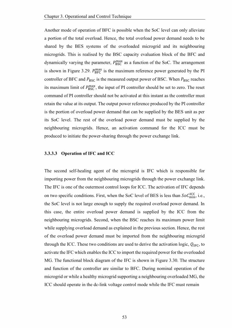
Chapter 3. Operational and Control Technique
53
Another mode of operation of BFC is possible when the SoC level can only alleviate
a portion of the total overload. Hence, the total overload power demand needs to be
shared by the BES systems of the overloaded microgrid and its neighbouring
microgrids. This is realised by the BSC capacity evaluation block of the BFC and
dynamically varying the parameter, 𝑃BSCmax as a function of the SoC. The arrangement
is shown in Figure 3.29. 𝑃BFCmax is the maximum reference power generated by the PI
controller of BFC and 𝑃BSC is the measured output power of BSC. When 𝑃BSC reaches
its maximum limit of 𝑃BSCmax, the input of PI controller should be set to zero. The reset
command of PI controller should not be activated at this instant as the controller must
retain the value at its output. The output power reference produced by the PI controller
is the portion of overload power demand that can be supplied by the BES unit as per
its SoC level. The rest of the overload power demand must be supplied by the
neighbouring microgrids. Hence, an activation command for the ICC must be
produced to initiate the power-sharing through the power exchange link.
3.3.3.3 Operation of IFC and ICC
The second self-healing agent of the microgrid is IFC which is responsible for
importing power from the neighbouring microgrids through the power exchange link.
The IFC is one of the outermost control loops for ICC. The activation of IFC depends
on two specific conditions. First, when the SoC level of BES is less than 𝑆𝑜𝐶minICC , i.e.,
the SoC level is not large enough to supply the required overload power demand. In
this case, the entire overload power demand is supplied by the ICC from the
neighbouring microgrids. Second, when the BSC reaches its maximum power limit
while supplying overload demand as explained in the previous section. Hence, the rest
of the overload power demand must be imported from the neighbouring microgrid
through the ICC. These two conditions are used to derive the activation logic, 𝑄IFC, to
activate the IFC which enables the ICC to import the required power for the overloaded
MG. The functional block diagram of the IFC is shown in Figure 3.30. The structure
and function of the controller are similar to BFC. During nominal operation of the
microgrid or while a healthy microgrid supporting a neighbouring overloaded MG, the
ICC should operate in the dc-link voltage control mode while the IFC must remain
Chapter 3. Operational and Control Technique
54
Inter-connection Frequency Controller (IFC)
ANDOR
delay tactIC
QSOC
QSOC
QIFC
+
+ANDPICC
dct
dct-PICC
+
+
ANDfmin
fMG
ANDdelay tdct
frc
R
S Q
Q
QICC
QICC
Flip-Flop
Comparator OL Detection & ICC Activation
Qdct
IC
QIFC
+
RESET PICC
max
0 Kic(1+sTic)sTic
Q ICC
QICC
LPF
s+ωic
ωic
PI MUX Limiter
0 -
fMG
fmin
OL Power Ref. Generationdelay tPIIFC
Compensator
DC Link Voltage Control
+(.)2Vdc
ref
(.)2Vdc
Kdc(s+ωz)s(s+ωp)
So
ICC Detection IFC Activation
0 MUX
SoQICC
PICC
OL
Pdc
QICC
PICCref
So
PICC
QCAP
Figure 3.30. Control mechanism of ICC for overload management
deactivated. However, if the healthy microgrid that was supporting an overloaded MG,
becomes overloaded too, the local BES system of the healthy microgrid and its BFC
should get activated to alleviate the overload situation as long as the overload power
is less than 𝑃BSCmax of that particular MG. If the overload power exceeds 𝑃BSC
max, then there
is no alternative other than to initiate load-shedding. This is achieved by the activation
logic of 𝑄ICC, as can be seen from Figure 3.30. A logic low value of 𝑄ICC indicates
that, the microgrid is already supporting another neighbouring overloaded microgrid
and the ICC must operate in the dc-link voltage control mode, while IFC should remain
deactivated. The steps of operation of the control approach in such a case can be
interpreted from the flowchart of Figure 3.28. The sequence of the control logic is
necessary to implement the developed decentralised control approach. Otherwise, the
interconnection among the microgrids will lead to instability throughout the entire
system.
Chapter 3. Operational and Control Technique
55
3.4 Comparison among the three topologies
In this study, it has been established that the power exchange amongst the microgrids
can be realised through any of the three topologies where each topology has its own
advantages or drawbacks. However, it should be noted that such links only enable
power exchange among the microgrids provisionally and during any contingency that
requires to exchange 10-20% of the total generation capacity of each microgrid. To
realise such interconnecting links that only carry a small amount of power for a short
duration, proper economical, feasible and most optimal option needs to be selected. It
is obvious that based on the distance among the microgrids and the amount of power
that is going to be shared will play the most important role in selecting the most optimal
topology for such interconnection. For microgrid clusters located in close proximity,
ac interconnection may be more suitable and economical whereas, if the distance is
large, then dc interconnection will be preferred. Furthermore, when selecting an ac
interconnecting link based on the above-mentioned criteria, a single-phase link can be
more suitable over a three-phase link or vice versa. A single-phase ac link of topology-
2, and a single-phase power electronics converter requires fewer components than a
three-phase ac link of topology-3. Also, the required number of current and voltage
sensors, closed-loop controllers, and signal processing circuitry is less. Nevertheless,
the computational effort for signal processing in a single-phase voltage source
converter is smaller compared to the three-phase converter. On the other hand,
employing a dc interconnection reduces the number of the required interlinking
converter by 50% and thus reducing the number of components required as well as the
computational effort of signal processing. Applying dc-link also eliminates the
complexity of synchronization of the converters to power exchange lines and the
operation of the power exchange link is more versatile, robust, and flexible. This
distinctive feature of the dc-link can be explained with the help of the presented
simulation results discussed in the time domain case studies of the three topologies.
A comparison among the three topologies is given in Table 3.2. In topology- 3, as the
number of switching devices, LCL filters, and conductors is less, the power losses in
these components will also be the minimum among all the three topologies, and a
better converter efficiency can be achieved. At the same time, the number of sensors
and LCL filters (the most expensive components of the converter) required for a dc-
link is 50% less than that of the three-phase link and 40% less than that of the single-

Chapter 3. Operational and Control Technique
56
Table 3.2 Comparison of different topologies employed for power exchange link
Parameters single-phase link three-phase link dc-link
No. of switching
devices 10 12 6
No. of LCL filters 4 6 3
No. of current sensors 8 12 6
No. of voltage sensors 8 12 6
Number of lines 1 3 2
phase link, and thus offers a substantial reduction in cost and size of the converter.
Finally, the number of conductors required in the single-phase link is one (assuming
earth neutral), whereas two and three conductors are required for dc and three-phase
ac link, respectively. However, the total power that can be exchanged in a single-phase
link is one-third of the three-phase link, whereas the maximum power that can be
exchanged for a given voltage level, is through the dc-link. If the same amount of
power needs to be transferred through a single-phase link, either the reference voltage
across the filter capacitor of 𝐶f needs to be increased or the size of the conductors needs
to be increased to minimise the line impedance (approximately, one-third than that of
three-phase lines). Also, the coupling inductance 𝐿g needs to be reduced to
accommodate the desired power flow. Each one of these solutions has its own
limitation. First, the voltage reference across 𝐶f cannot be made very large as it may
produce excess stress over the switching devices and the other components and thus
may incur an additional cost. Also, the voltage across 𝐶f is related to the dc-link voltage
of the converter as its value should be less than half of the dc-link voltage to avoid
saturation. Second, using conductors with a larger cross-section area would make the
system and its transmission structures more expensive. Third, 𝐿g cannot be made very
small as the switching harmonics may not get properly filtered out and can cause
harmonic distortion in the output voltage waveform. At the same time, the modified
angle droop with virtual impedance is employed to ensure the desired power-sharing
among the HMGs. To implement such a droop control scheme, 𝐿g needs to be large
enough to decouple the active and reactive power-sharing and needs to be larger than
a certain minimum value. Otherwise, it may deteriorate the property of power-sharing
based on droop coefficients.
The main purpose of using a single-phase ac link over a three-phase link to couple
microgrids is to reduce the cost as the number of equipment and interconnecting lines
will be less. However, this is valid in the case of autonomous microgrids which are
Chapter 3. Operational and Control Technique
57
located close to each other in a certain geographical area. If the distance among the
microgrids is large, then the benefits of the single-phase links over three-phase links
may not be applicable anymore. Using dc-link to couple microgrids can be more
feasible but, the protection equipment for dc system are expensive compare to ac
system up to some extent. Also, the majority of the power distribution line
infrastructure and commercially available equipment are based on ac systems. At the
same time, the network operators are usually more accustomed to ac distribution
systems as compared to dc systems. Moreover, dc systems would be more economical
or cost-effective if the distance among the microgrids is long.
3.5 Summary
This chapter presented the technique and control mechanism of coupling neighbouring
microgrids to exchange power amongst them. The designed controller and its
frequency response characteristics are discussed. A detailed explanation of
coordinating between different mode of operation of the converters and their
controllers are presented. The performances of each of these techniques are validated
through time-domain simulation and numerical analyses in the following chapters.
Chapter 4. Time Domain Analysis
58
Chapter 4 Time Domain Analysis
This chapter presents the time domain simulation used for demonstrating and
validating the performance of the proposed control mechanism. Several case studies
have been developed for a sample network made up individually using the three
proposed topologies in which uncertainties in the generation of the renewable sources
or load demand result in overloading or over-generation leading to unacceptable
frequency and voltage deviation. It has been demonstrated in this chapter that the
proposed control mechanism can successfully alleviate the overloading and over-
generation problems and retain the voltage and frequency. The chapter also presents a
comparative analysis of the performance of the three proposed topologies.
4.1 Network Under Consideration
Let Consider a network of Figure 1.1 where 3 autonomous microgrids, each consisting
of several DERs, distributed generators, loads, and one interlinking converter coupled
to a power exchange link. The interlinking converter can be any one of the three
topologies shown in Figure 1.2. The DERs are connected to the microgrid through
VSCs which are controlled in different operating modes to regulate the power and
frequency of each microgrid. The DERs are assumed to be operating in the 𝑃 − 𝑓 and
𝑄 − 𝑉 droop control modes, where the voltage and frequency at the output of each
DER is determined from [73]
4.2 Performance Evaluation
To evaluate the dynamic performance of the proposed control technique for all the
three topologies, let us consider the system of Fig. 1.1 with 3 microgrids that have
formed a CMG through a common power exchange link and power electronic
Chapter 4. Time Domain Analysis
59
converters where every individual microgrid is operating under the droop control
technique mentioned in Section 2.1. The power exchange link can be any one of the
three proposed topologies as discussed in chapter 3. The performance of such a system
with every topology has been evaluated under various conditions, i.e., the normal,
overloaded, and over-generating, using different case studies. Each microgrid is
operating under a voltage and frequency droop while the technical parameters of the
network under consideration and the controllers are provided in Table 4.1. The time-
domain results of the study are presented in this chapter. The results show the
frequency of each microgrid and the injected/absorbed power from/to one microgrid
to the interconnecting lines (measured at the output of their corresponding LSCs).
These figures also illustrate the dc-link voltage within the back-to-back converter
(topology -1 and 2) or VSC (topology-3 and battery storage and CMG coordination),
as well as the reference power and the voltage angle at the output of the LSCs. The
transition of the control of the LSCs from droop to constant PQ mode and vice versa
is also illustrated.
4.2.1 Topology-1 (Three-phase ac link)
The performance of proposed topology-1 is evaluated using two different case studies.
In the first case study, the microgrids are overloaded or experiencing overgeneration
separately whereas in the second case, overloading and overgeneration scenario are
created simultaneously. The objective of these case studies is to validate the efficacy
of the power exchange mechanism which demonstrates that, both overloading or over-
generation problems can be addressed effectively, and the injected/absorbed power is
shared based on the MG’s droop ratio
4.2.1.1 Case Study-1 (Separate overloaded and over-generating PMG)
In this case study first MG-1 has become provisionally overloaded; thus, the other two
HMGs (i.e., MG-2 and 3) successfully support MG-1 by supplying the required power
demand under the proposed power exchange and control strategy. After a certain
period, overloading in MG-1 is over and all the three microgrids operate as HMGs.
Later, MG-3 starts experiencing over-generation, and hence, MG-1 and MG-2 start
Chapter 4. Time Domain Analysis
60
Table 4.1 Technical data of network under consideration
Network 𝑉rated = 415V, 𝑓nom = 50Hz, 𝑓min = 49.5Hz, 𝑓max = 50.2Hz, 𝑃max = 100kW,
𝑉dc = 1.5kV, 𝑍MG = 0.1 + 𝑗0.5Ω, 𝑍line = 0.1 + 𝑗0.08Ω
DER droop 𝑚 = 0.01Hz/kW, 𝑛 = 0.1V/kVAR
Angle droop 𝑚d = 0.002 rad/kW, 𝑛d = 0.004V/kVAR
DC Droop
Parameters
𝑚MG−1 = 2.5V/kW, 𝑚MG−2 = 5V/kW, 𝑚MG−3 = 5V/kW
VSC and filters 𝑅f = 0.1Ω, 𝐿f = 2mH, 𝑅g(MSC) = 0.04Ω, 𝐿𝑔(MSC) = 1.36mH, 𝑅g(LSC) = 0.12Ω,
𝐿𝑔(LSC) = 10mH, 𝐶f = 25μF, 𝐶dc = 4700μF
Linear quadratic
regulator gains
𝑘1 = 58.63, 𝑘2 = 97.18, 𝑘3 = 1.2, 𝜔𝑐 = 6283.2 rad/s
PI - PQ
controller (MSC)
Proportional Gain, 𝐾c = 0.628, Time Constant, 𝑇c = 0.034 s, 𝑓BW = 73.5Hz
PI - PQ
controller (LSC)
Proportional Gain, 𝐾c = 0.628, Time Constant, 𝑇c = 0.0834 s, 𝑓BW = 10Hz
Frequency
controller
𝐾OL = 15k, 𝑇OL = 0.025 s, 𝜔OL = 314 rad/s, 𝐾OG = 20k, 𝑇OG = 0.05 s, 𝜔OG = 37.7
krad/s
𝐾PLL = 5, 𝑇PLL = 0.02 s
Dc-link voltage
controller 𝐾dc = 222, 𝜔z = 2.2rad/s, 𝜔p = 1000rad/s, 𝜏dc = 392.2ms, 𝑃so = 100kW, 𝑉d =
380V
absorbing the excess power from it to maintain its minimum or baseload power
demand.
Initially, all microgrids are assumed to be operating at the steady-state condition and
under the droop control mode with zero power exchange as all the microgrids are
HMGs. At, 𝑡 = 𝑡1, MG-1 becomes overloaded by 20% (see Figure. 4.1a); hence, its
frequency decreases from 49.8 to 49.3 Hz (see Figure. 4.1c). which is below the
acceptable limit of 49.5 Hz and thus, MG-1 becomes a PMG. The frequency controller
of MG-1 senses this situation and switches its mode of operation from droop to
constant PQ control after a certain time delay (i.e., 0.6 s). Hence, the OLFC gets
activated and determines the amount of power that needs to be supplied to MG-1 to
retain its frequency back to the acceptable limit. Thus at 𝑡 = 𝑡2, MG-2 and MG-3 start
injecting the required power of 0.155 and 0.076 pu as demanded by MG-1,
respectively. The share of power between MG-2 and MG-3 is determined by the
assumed (desired) droop ratio (i.e., 1: 2 in this case); thus, the power delivered by MG-
2 is twice that of MG-3, as seen from Figure. 4.1b.
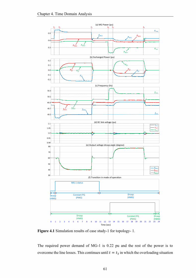
Chapter 4. Time Domain Analysis
61
(a) MG Power (pu)
0 1 2 3 4 5 6 7 8 9 10 11 12
PMG1
PMG2 PMG3
0.0
0.1
0.2
-0.1
-0.2
(b) Exchanged Power (pu)
Pg3
Pg1
49.5
49.7
49.9
50.1
60
(c) Frequency (Hz)
1.0
1.05
1.1
0.95
0.90
(d) DC link voltage (pu)
fMG2fMG3 fMG1
(e) Output voltage droop angle (degree)
(f) Transition in mode of operation
MG-1 status
Droop (HMG)
Constant PQ (PMG)
Droop (HMG)
t1 t2 t3
Pg2Pg2
13 14 15 16 17 18 19 20 21 22 23 24
Droop (HMG)
Constant PQ (PMG)
Droop (HMG)
Time (sec)
Pg1
Pg3
PMG3
PMG1PMG2
50.3
0.3
0.9
0.6
t4 t5 t6
Vdc1
Vdc2
Vdc3
70
80
50
40
30
δMG1 δMG2 δMG3
Pmax
Pmin
fmax
fmin
Figure 4.1 Simulation results of case study-1 for topology- 1.
The required power demand of MG-1 is 0.22 pu and the rest of the power is to
overcome the line losses. This continues until 𝑡 = 𝑡3 in which the overloading situation
Chapter 4. Time Domain Analysis
62
Table 4.2 Events applied to microgrids in Case study-1 at different intervals
Time
Instant
MG Status Action taken
MG-1 MG-2 MG-3
𝑡1 OL HMG HMG Normal operation for MG-2 and MG-3 while MG-1 is
overloaded.
𝑡2 PMG HMG HMG MG-1 is overloaded while MG-2 and MG-3 are
supporting it by supplying the overload power.
𝑡3 HMG HMG HMG Over-generation of MG-1 is over, and all MGs become
HMG.
𝑡4 HMG HMG OG Normal operation for MG-1 and MG-2 while MG-3 is
over-generating.
𝑡5 HMG HMG PMG MG-3 over-generating while MG-1 and MG-2 are
supporting it by absorbing the excess power.
𝑡6 HMG HMG HMG Over-generation of MG-3 is over, and all MGs become
HMG.
is alleviated. At 𝑡 = 𝑡3 the overload is removed, and as soon as this occurs, the
frequency of MG-1 increases to 49.8 Hz (i.e., above the level of minimum acceptable
limit). Therefore, MG-1 goes back to its nominal operating condition and becomes an
HMG. Hence, MG-2 and MG-3 cease to supply power to MG-1. After the MG-1 settles
back as HMG and steady-state condition is reached, the frequency controller of MG-1
switches its mode of operation from constant PQ to droop control as can be seen from
Figure. 4.1f. At 𝑡 = 𝑡4, MG-3 experiences an excessive power generation by 18% (see
Figure. 4.1a), and its frequency increases from 49.94 to 50.36 Hz (see Figure. 4.1c).
As the frequency has increased beyond the acceptable limit of 50.2 Hz, MG-3 becomes
a PMG. Thus, the frequency controller of MG-3 senses the situation and switches its
mode of operation from droop to constant PQ control after a certain predefined time
delay (i.e., 0.6 s). Hence, the OGFC gets activated and determines the amount of power
that needs to be exported from MG-3 to retain its frequency back to the acceptable
limit. Thus at 𝑡 = 𝑡5, MG-1 and MG-2 start absorbing the required power of 0.121 and
0.062 pu, respectively. The power-sharing between MG-1 and MG-2 is maintained as
1: 2, as seen from Figure. 4.1b. The power delivered by MG-3 is 0.195 pu. This
continues until 𝑡 = 𝑡6 in which the situation of excessive generation in MG-3 is
alleviated and the frequency of MG-3 decreases to 49.94 Hz (i.e., below the level of
the maximum acceptable limit of 50.2 Hz). Therefore, MG-3 goes back to its nominal
operating condition and becomes an HMG. Hence, MG-1 and MG-2 cease to absorb
power form MG-3. After MG-3 settles back as HMG and steady-state condition is
attained, the frequency controller of MG-3 switches its mode of operation from
constant PQ to droop control. Table 4.2 summarises the events applied to the
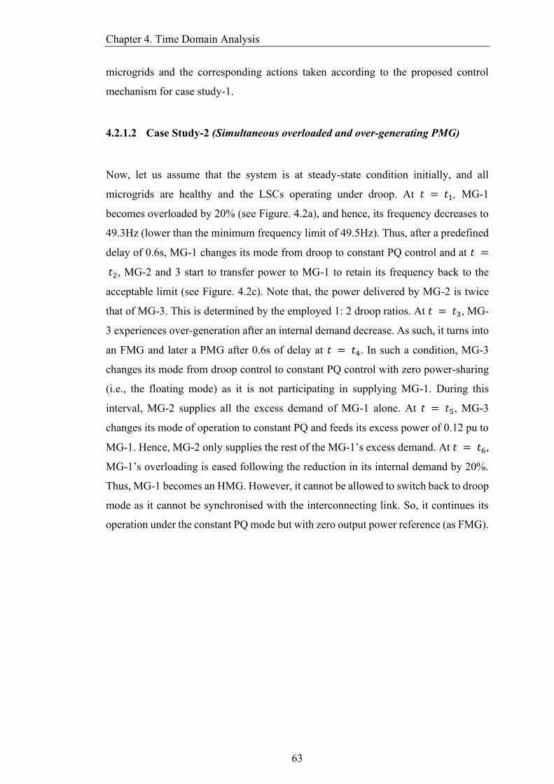
Chapter 4. Time Domain Analysis
63
microgrids and the corresponding actions taken according to the proposed control
mechanism for case study-1.
4.2.1.2 Case Study-2 (Simultaneous overloaded and over-generating PMG)
Now, let us assume that the system is at steady-state condition initially, and all
microgrids are healthy and the LSCs operating under droop. At 𝑡 = 𝑡1, MG-1
becomes overloaded by 20% (see Figure. 4.2a), and hence, its frequency decreases to
49.3Hz (lower than the minimum frequency limit of 49.5Hz). Thus, after a predefined
delay of 0.6s, MG-1 changes its mode from droop to constant PQ control and at 𝑡 =
𝑡2, MG-2 and 3 start to transfer power to MG-1 to retain its frequency back to the
acceptable limit (see Figure. 4.2c). Note that, the power delivered by MG-2 is twice
that of MG-3. This is determined by the employed 1: 2 droop ratios. At 𝑡 = 𝑡3, MG-
3 experiences over-generation after an internal demand decrease. As such, it turns into
an FMG and later a PMG after 0.6s of delay at 𝑡 = 𝑡4. In such a condition, MG-3
changes its mode from droop control to constant PQ control with zero power-sharing
(i.e., the floating mode) as it is not participating in supplying MG-1. During this
interval, MG-2 supplies all the excess demand of MG-1 alone. At 𝑡 = 𝑡5, MG-3
changes its mode of operation to constant PQ and feeds its excess power of 0.12 pu to
MG-1. Hence, MG-2 only supplies the rest of the MG-1’s excess demand. At 𝑡 = 𝑡6,
MG-1’s overloading is eased following the reduction in its internal demand by 20%.
Thus, MG-1 becomes an HMG. However, it cannot be allowed to switch back to droop
mode as it cannot be synchronised with the interconnecting link. So, it continues its
operation under the constant PQ mode but with zero output power reference (as FMG).
Chapter 4. Time Domain Analysis
64
(a) MG Power (pu)
PMG1
0.2
0.6
1
1.4
PMG2
PMG3
PMG1
Load
PMG3
Load
Pg1
Pg2
Pg3
0
0.2
0.1
-0.2
-0.1
(b) Exchanged Power (pu)
50
50.4
49.6
49.2
(d) DC link voltage (pu)
fMG1
fMG2
fMG3
1
1.1
0.9
(c) Frequency (Hz)
Vdc1
Vdc2
Vdc3
0
0.2
0.1
-0.1
(e) Reference power tracking (pu)
Pg1ref Pg3
ref
Pg1 Pg3
60
80
40
20
(f) Output voltage angle (degree)
δMG1 δMG2 δMG3
MG-1
MG-3
Droop(HMG)
Constant PQ (PMG) Droop(HMG)
Constant PQ (PMG)Droop(HMG)
Droop(HMG)
Time (sec)
(g) Mode transition Control Signal
0 1 2 3 4 5 6 7 8 9 10 11 12 13 14
0 1 2 3 4 5 6 7 8 9 10 11 12 13 14
0 1 2 3 4 5 6 7 8 9 10 11 12 13 14
0 1 2 3 4 5 6 7 8 9 10 11 12 13 14
0 1 2 3 4 5 6 7 8 9 10 11 12 13 14
0 1 2 3 4 5 6 7 8 9 10 11 12 13 14
0 1 2 3 4 5 6 7 8 9 10 11 12 13 14
t1 t2 t3 t5t4 t6 t7
Figure 4.2 Simulation results of case study-2 for topology- 1.
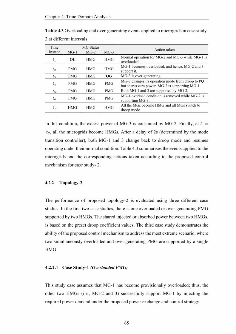
Chapter 4. Time Domain Analysis
65
Table 4.3 Overloading and over-generating events applied to microgrids in case study-
2 at different intervals
Time
Instant
MG Status Action taken
MG-1 MG-2 MG-3
𝑡1 OL HMG HMG Normal operation for MG-2 and MG-3 while MG-1 is
overloaded.
𝑡2 PMG HMG HMG MG-1 becomes overloaded, and hence, MG-2 and 3
support it.
𝑡3 PMG HMG OG MG-3 is over-generating.
𝑡4 PMG HMG FMG MG-3 changes its operation mode from droop to PQ
but shares zero power. MG-2 is supporting MG-1.
𝑡5 PMG HMG PMG Both MG-1 and 3 are supported by MG-2.
𝑡6 FMG HMG PMG MG-1 overload condition is removed while MG-2 is
supporting MG-3.
𝑡7 HMG HMG HMG All the MGs become HMG and all MGs switch to
droop mode.
In this condition, the excess power of MG-3 is consumed by MG-2. Finally, at 𝑡 =
𝑡7, all the microgrids become HMGs. After a delay of 2s (determined by the mode
transition controller), both MG-1 and 3 change back to droop mode and resumes
operating under their normal condition. Table 4.3 summarises the events applied to the
microgrids and the corresponding actions taken according to the proposed control
mechanism for case study- 2.
4.2.2 Topology-2
The performance of proposed topology-2 is evaluated using three different case
studies. In the first two case studies, there is one overloaded or over-generating PMG
supported by two HMGs. The shared injected or absorbed power between two HMGs,
is based on the preset droop coefficient values. The third case study demonstrates the
ability of the proposed control mechanism to address the most extreme scenario, where
two simultaneously overloaded and over-generating PMG are supported by a single
HMG.
4.2.2.1 Case Study-1 (Overloaded PMG)
This study case assumes that MG-1 has become provisionally overloaded; thus, the
other two HMGs (i.e., MG-2 and 3) successfully support MG-1 by injecting the
required power demand under the proposed power exchange and control strategy.
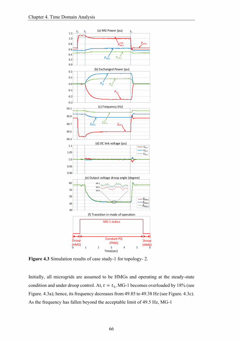
Chapter 4. Time Domain Analysis
66
(a) MG Power (pu)
0.2
0.6
1.0
0.4
0.8
1.2
PMG1
PMG2
PMG1Load
PMG3
0.0
0.0
0.1
0.2
-0.1
-0.2
-0.3
(b) Exchanged Power (pu)
Pg3
Pg1
49.5
49.7
49.9
50.1
49.3
(c) Frequency (Hz)
1.0
1.05
1.1
0.95
0.90
(d) DC link voltage (pu)
fMG2fMG3 fMG1
Vdc1
Vdc2
Vdc3
60
55
40
45
50
(e) Output voltage droop angle (degree)
(f) Transition in mode of operation
MG-1 status
Droop (HMG)
Constant PQ (PMG)
Droop (HMG)
δMG1 δMG2 δMG3
t1 t2 t3
Pg2
Time(sec)0 1 2 3 4 5 6
45.8
46.0
46.2
Figure 4.3 Simulation results of case study-1 for topology- 2.
Initially, all microgrids are assumed to be HMGs and operating at the steady-state
condition and under droop control. At, 𝑡 = 𝑡1, MG-1 becomes overloaded by 18% (see
Figure. 4.3a); hence, its frequency decreases from 49.85 to 49.38 Hz (see Figure. 4.3c).
As the frequency has fallen beyond the acceptable limit of 49.5 Hz, MG-1
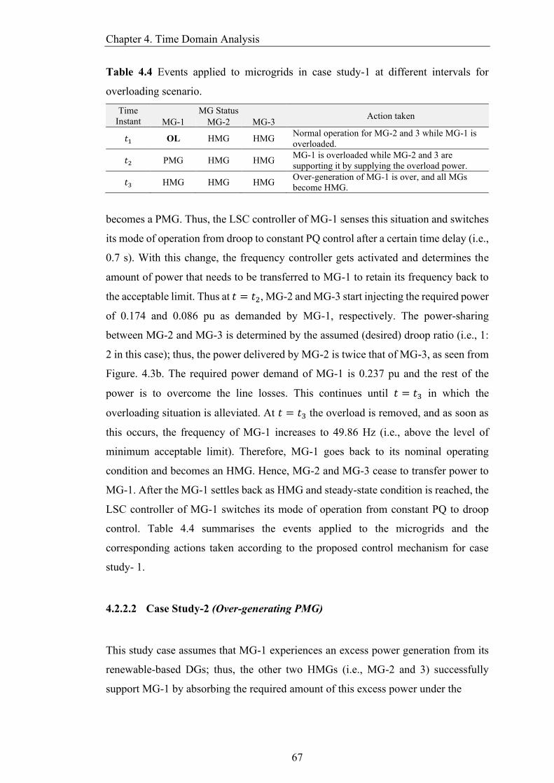
Chapter 4. Time Domain Analysis
67
Table 4.4 Events applied to microgrids in case study-1 at different intervals for
overloading scenario.
Time
Instant
MG Status Action taken
MG-1 MG-2 MG-3
𝑡1 OL HMG HMG Normal operation for MG-2 and 3 while MG-1 is
overloaded.
𝑡2 PMG HMG HMG MG-1 is overloaded while MG-2 and 3 are
supporting it by supplying the overload power.
𝑡3 HMG HMG HMG Over-generation of MG-1 is over, and all MGs
become HMG.
becomes a PMG. Thus, the LSC controller of MG-1 senses this situation and switches
its mode of operation from droop to constant PQ control after a certain time delay (i.e.,
0.7 s). With this change, the frequency controller gets activated and determines the
amount of power that needs to be transferred to MG-1 to retain its frequency back to
the acceptable limit. Thus at 𝑡 = 𝑡2, MG-2 and MG-3 start injecting the required power
of 0.174 and 0.086 pu as demanded by MG-1, respectively. The power-sharing
between MG-2 and MG-3 is determined by the assumed (desired) droop ratio (i.e., 1:
2 in this case); thus, the power delivered by MG-2 is twice that of MG-3, as seen from
Figure. 4.3b. The required power demand of MG-1 is 0.237 pu and the rest of the
power is to overcome the line losses. This continues until 𝑡 = 𝑡3 in which the
overloading situation is alleviated. At 𝑡 = 𝑡3 the overload is removed, and as soon as
this occurs, the frequency of MG-1 increases to 49.86 Hz (i.e., above the level of
minimum acceptable limit). Therefore, MG-1 goes back to its nominal operating
condition and becomes an HMG. Hence, MG-2 and MG-3 cease to transfer power to
MG-1. After the MG-1 settles back as HMG and steady-state condition is reached, the
LSC controller of MG-1 switches its mode of operation from constant PQ to droop
control. Table 4.4 summarises the events applied to the microgrids and the
corresponding actions taken according to the proposed control mechanism for case
study- 1.
4.2.2.2 Case Study-2 (Over-generating PMG)
This study case assumes that MG-1 experiences an excess power generation from its
renewable-based DGs; thus, the other two HMGs (i.e., MG-2 and 3) successfully
support MG-1 by absorbing the required amount of this excess power under the
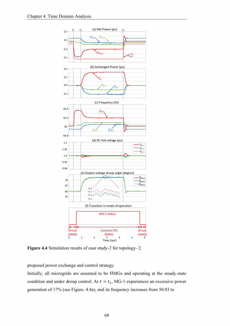
Chapter 4. Time Domain Analysis
68
Pg2
0.1
0.3
0.5
0.7(a) MG Power (pu)
(b) Exchanged Power (pu)
(c) Frequency (Hz)
(d) DC link voltage (pu)
(e) Output voltage droop angle (degree)
(f) Transition in mode of operation
0.0
0.1
0.2
-0.1
50.2
50.4
50
49.8
1.0
1.05
1.1
0.95
0.90
60
70
65
55
Droop (HMG)
Constant PQ (PMG)
Droop (HMG)
Time (sec)
PMG1LoadPMG1
PMG2 PMG3
Pg1
Pg3
fMG1
fMG3 fMG2
Vdc1
Vdc2
Vdc3
t1 t2 t3
δMG1 δMG2 δMG3
0 1 2 3 4 5 6
72.7
72.3
72.5
72.9
MG-1 status
Figure 4.4 Simulation results of case study-2 for topology- 2.
proposed power exchange and control strategy.
Initially, all microgrids are assumed to be HMGs and operating at the steady-state
condition and under droop control. At 𝑡 = 𝑡1, MG-1 experiences an excessive power
generation of 17% (see Figure. 4.4a), and its frequency increases from 50.03 to
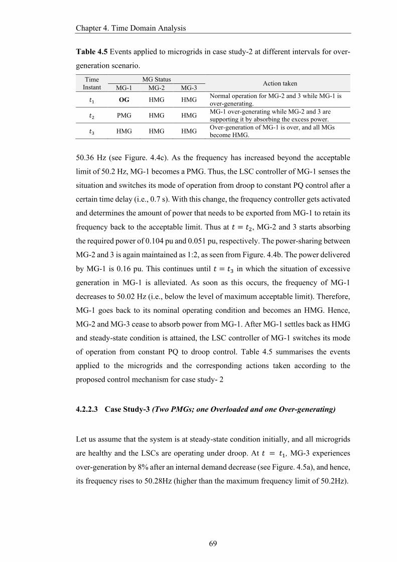
Chapter 4. Time Domain Analysis
69
Table 4.5 Events applied to microgrids in case study-2 at different intervals for over-
generation scenario.
Time
Instant
MG Status Action taken
MG-1 MG-2 MG-3
𝑡1 OG HMG HMG Normal operation for MG-2 and 3 while MG-1 is
over-generating.
𝑡2 PMG HMG HMG MG-1 over-generating while MG-2 and 3 are
supporting it by absorbing the excess power.
𝑡3 HMG HMG HMG Over-generation of MG-1 is over, and all MGs
become HMG.
50.36 Hz (see Figure. 4.4c). As the frequency has increased beyond the acceptable
limit of 50.2 Hz, MG-1 becomes a PMG. Thus, the LSC controller of MG-1 senses the
situation and switches its mode of operation from droop to constant PQ control after a
certain time delay (i.e., 0.7 s). With this change, the frequency controller gets activated
and determines the amount of power that needs to be exported from MG-1 to retain its
frequency back to the acceptable limit. Thus at 𝑡 = 𝑡2, MG-2 and 3 starts absorbing
the required power of 0.104 pu and 0.051 pu, respectively. The power-sharing between
MG-2 and 3 is again maintained as 1:2, as seen from Figure. 4.4b. The power delivered
by MG-1 is 0.16 pu. This continues until 𝑡 = 𝑡3 in which the situation of excessive
generation in MG-1 is alleviated. As soon as this occurs, the frequency of MG-1
decreases to 50.02 Hz (i.e., below the level of maximum acceptable limit). Therefore,
MG-1 goes back to its nominal operating condition and becomes an HMG. Hence,
MG-2 and MG-3 cease to absorb power from MG-1. After MG-1 settles back as HMG
and steady-state condition is attained, the LSC controller of MG-1 switches its mode
of operation from constant PQ to droop control. Table 4.5 summarises the events
applied to the microgrids and the corresponding actions taken according to the
proposed control mechanism for case study- 2
4.2.2.3 Case Study-3 (Two PMGs; one Overloaded and one Over-generating)
Let us assume that the system is at steady-state condition initially, and all microgrids
are healthy and the LSCs are operating under droop. At 𝑡 = 𝑡1, MG-3 experiences
over-generation by 8% after an internal demand decrease (see Figure. 4.5a), and hence,
its frequency rises to 50.28Hz (higher than the maximum frequency limit of 50.2Hz).
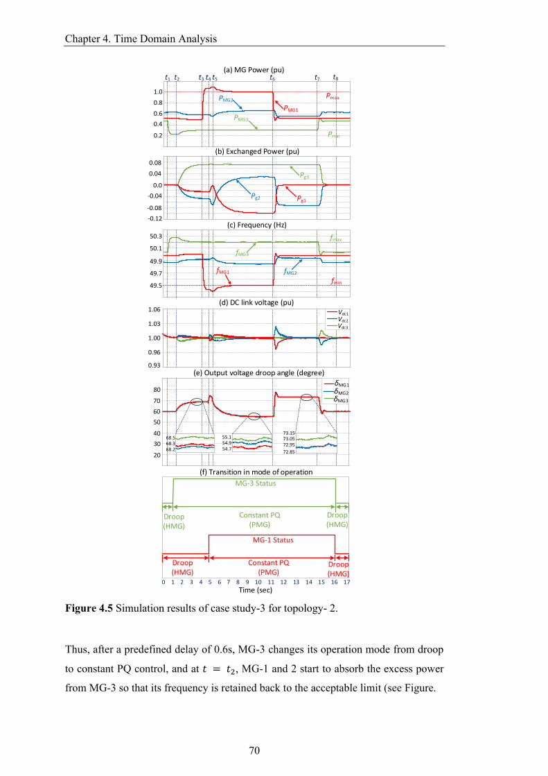
Chapter 4. Time Domain Analysis
70
1.0
55.154.954.7
73.1573.0572.95
72.85
68.568.368.2
(f) Transition in mode of operation
Constant PQ (PMG)
Droop (HMG)
Droop (HMG)
Droop (HMG)
Droop (HMG)
Constant PQ (PMG)
0 1 2 3 4 5 6 7 8 9 10 11 12 13 14 15 16 17
Time (sec)
t2t1 t3 t4 t5 t6 t7
(a) MG Power (pu)
0.6
0.8
0.2
0.4
(b) Exchanged Power (pu)
0.0
0.08
0.04
-0.04
-0.08
-0.12(c) Frequency (Hz)
49.5
49.7
49.9
50.1
50.3
(d) DC link voltage (pu)
1.00
1.03
1.06
0.96
0.93(e) Output voltage droop angle (degree)
60
70
80
50
40
30
20
PMG1
PMG2
PMG3
Pmax
Pmin
Pg1Pg2
Pg3
fMG3
fMG1 fMG2
Vdc1
Vdc2
Vdc3
δMG1 δMG2 δMG3
fmin
fmax
t8
MG-3 Status
MG-1 Status
Figure 4.5 Simulation results of case study-3 for topology- 2.
Thus, after a predefined delay of 0.6s, MG-3 changes its operation mode from droop
to constant PQ control, and at 𝑡 = 𝑡2, MG-1 and 2 start to absorb the excess power
from MG-3 so that its frequency is retained back to the acceptable limit (see Figure.
Chapter 4. Time Domain Analysis
71
Table 4.6 Overloading and over-generating events applied to microgrids in case study-
3 at different intervals.
Time
Instant
MG Status Action taken
MG-1 MG-2 MG-3
𝑡1 HMG HMG OG Normal operation for MG-1 and MG-2 while MG-3 is
over-generating.
𝑡2 HMG HMG PMG MG-3 becomes over-generating, and hence, MG-1 and
2 support it.
𝑡3 OL HMG PMG MG-1 is overloaded.
𝑡4 FMG HMG PMG MG-1 changes its operation mode from droop to PQ but
shares zero power. MG-2 is supporting MG-3.
𝑡5 PMG HMG PMG Both MG-1 and 3 are supported by MG-2.
𝑡6 FMG HMG PMG MG-1’s overload condition is removed while MG-2 is
supporting MG-3.
𝑡7 FMG HMG FMG MG-3’s over-generation is over and both MG-1 and
MG-3 are in PQ mode with zero power-sharing
𝑡8 HMG HMG HMG All MGs become HMG and all MGs switch to droop
mode.
4.5c). Note that, the power delivered by MG-2 (𝑃𝑔2 = −0.0474 pu) is twice that of
MG-1 (𝑃𝑔1 = −0.024 pu). This is determined by the employed 1: 2 droop ratios
between these microgrids (see Figure. 4.5b). At 𝑡 = 𝑡3, MG-1 becomes overloaded
by 10% and its frequency falls to 49.4 Hz. As such, it turns into an FMG and later a
PMG after 0.6s of delay at 𝑡 = 𝑡4. In such a condition, MG-1 changes its operation
mode from droop control to constant PQ control with zero power-sharing (i.e., the
floating mode) as it is not participating in absorbing any excess power from MG-3.
During this interval, MG-2 absorbs all excess power of MG-3 alone. At 𝑡 = 𝑡5, MG-
1 starts to receive power from both over-generating PMG of MG-3 and HMG of MG-
2. First, MG-1 absorbs the total over-generating power (𝑃𝑔3 = 0.075 pu) of MG-3 and
the rest of the overload demand is supplied by MG-2 (𝑃𝑔2 = 0.025 pu) to retain MG-
1’s frequency back to the minimum limit of 49.5Hz. At 𝑡 = 𝑡6, MG-1’s overloading
is eased following the reduction in its internal demand by 10%. Thus, MG-1 becomes
an HMG. However, it cannot be allowed to switch back to droop mode as it cannot be
synchronised with the interconnecting link. So, it continues its operation under the
constant PQ mode but with zero output power reference (as an FMG). In this condition,
the excess power of MG-3 is consumed by MG-2 only. Finally, at 𝑡 = 𝑡7, the over-
generation of MG-3 is over and all microgrids become HMGs, but both MG-1 and
MG-3 will continue to operate as FMG until the droop angle of the interconnecting
lines returns back to 𝛿o. Once the desired value of 𝛿o is attained, indicating that, there
is no power exchange taking place in the link (i.e., all microgrids are HMGs), and after

Chapter 4. Time Domain Analysis
72
a preset delay of 2s (determined by the mode transition controller), both MG-1 and 3
change their operation mode back to droop mode. All microgrids resume operating
under their normal condition with no power flow in the power exchange link. Table
4.6 summarises the events applied to the microgrids and the corresponding actions
taken according to the proposed control mechanism for study case- 3.
4.2.3 Topology-3
The performance of proposed topology-3 is evaluated using two different case studies
under both balanced (case-1) and unbalanced (case-2) loading condition of CMG. In
both case studies, two PMGs (one overloaded and one over-generating) are supported
by one HMG. The purpose of this case study is to demonstrate the capability and
efficacy of the proposed power exchange mechanism in alleviating overloading/over-
generation scenario even when the microgrids are heavily unbalanced.
4.2.3.1 Case Study-1 (Balanced CMG)
Initially let us assume the system is at the steady-state condition and all the microgrids
are at the HMG mode. Therefore, the VSCs of all HMGs are operating under the dc
voltage droop control mode (i.e. their output power is zero and the voltage at their dc-
link is 1 pu); thus, there is no power flow in the power exchange dc-link.
Referring to Figure 4.6, At 𝑡 = 𝑡1, MG-3 becomes overloaded by 17%, and hence, its
frequency drops to 49.33 Hz (i.e., below the frequency limit of 49.5 Hz) while the
other two microgrids are still at the mode of operation from dc voltage droop control
to constant PQ mode, requesting an active power demand of 0.167 pu to alleviate the
overloading situation. As a result, at 𝑡 = 𝑡2, the other two HMGs start to support MG-
3 by injecting the required demand after a pre-defined delay of 0.6 s. MG-2 supplies
0.065 pu of power while MG-1 provides 0.122 pu which is twice that of MG-2 because
of the preset ratio of droop coefficients (𝑚MG-2/𝑚MG-1 = 2: 1) and thus, the frequency
of MG-3 is retained back to the desired limit of 49.5 Hz. This continues until 𝑡 = 𝑡3
at which MG-2 experiences excess-generation, and thus, its frequency rises and settles
at 50.35 Hz (beyond the acceptable limit of 50.3 Hz in this particular
Chapter 4. Time Domain Analysis
73
0.0
Frequency (Hz)
Exchanged Power (pu)
DC link voltage (pu)
Reference Power Tracking (pu)
Mode Transition Signals
0 1 2 3 4 5 6 7 8 9 10 11 12 13 14 15
MG-2 status
Droop (HMG)
Constant PQ (PMG)
Droop (HMG)
PMG1
PMG2
PMG3
LoadPMG2
LoadPMG2
fMG1
fMG2
fMG3
Pg1
Pg2
Pg3
Vdc1
Vdc2
Vdc3
PMG2 PMG3
Pref2 Pref3
MG-3 status
Droop (HMG)
Constant PQ (PMG)
Droop (HMG)
t1 t2 t3 t4 t5 t6 t7 t8
0.4
0.8
1.2
50
50.2
49.8
50.4
49.6
49.4
0.0
0.1
0.2
-0.1
-0.2
0.0
0.1
0.2
-0.1
1.0
0.96
0.92
1.04
MG Power (pu)
Figure 4.6 Simulation results of case study-1 for topology- 3.
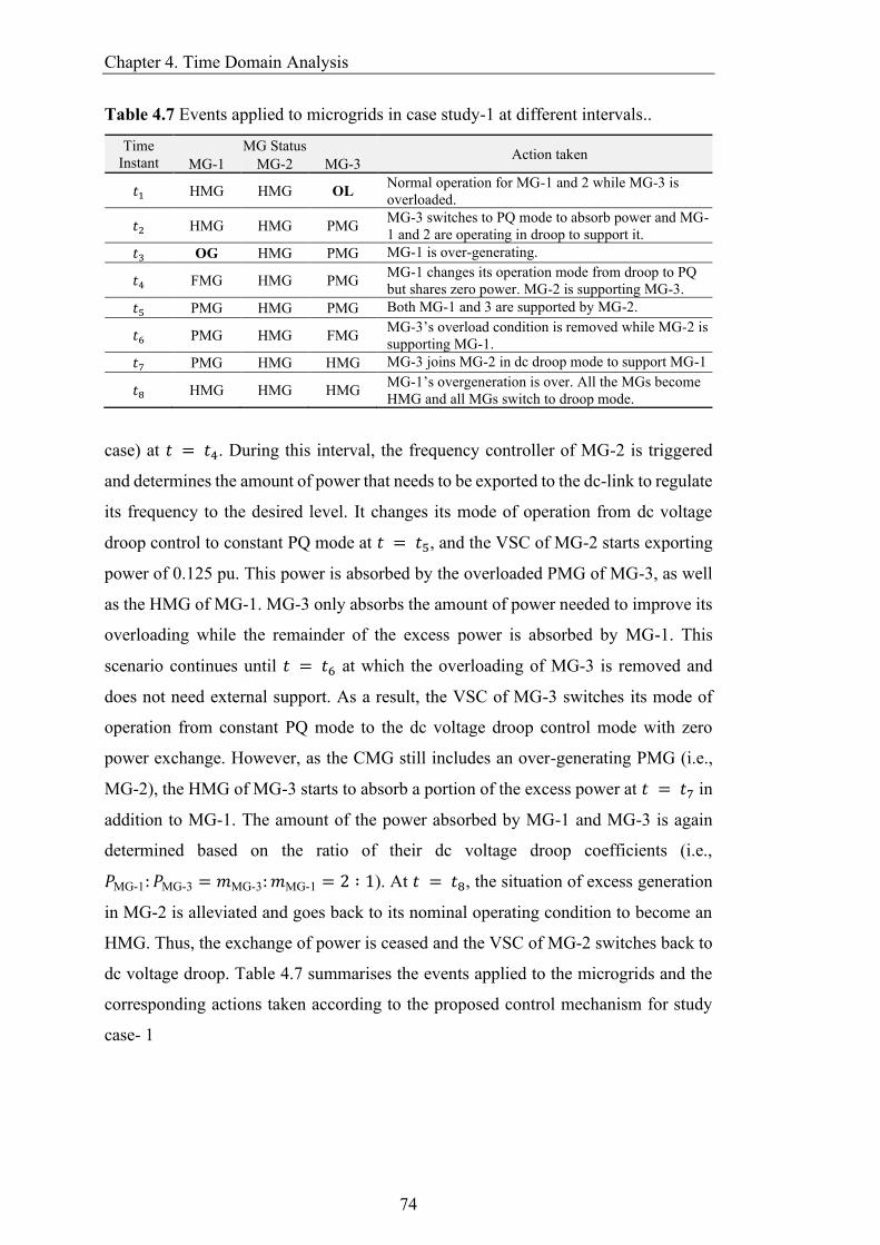
Chapter 4. Time Domain Analysis
74
Table 4.7 Events applied to microgrids in case study-1 at different intervals..
Time
Instant
MG Status Action taken
MG-1 MG-2 MG-3
𝑡1 HMG HMG OL Normal operation for MG-1 and 2 while MG-3 is
overloaded.
𝑡2 HMG HMG PMG MG-3 switches to PQ mode to absorb power and MG-
1 and 2 are operating in droop to support it.
𝑡3 OG HMG PMG MG-1 is over-generating.
𝑡4 FMG HMG PMG MG-1 changes its operation mode from droop to PQ
but shares zero power. MG-2 is supporting MG-3.
𝑡5 PMG HMG PMG Both MG-1 and 3 are supported by MG-2.
𝑡6 PMG HMG FMG MG-3’s overload condition is removed while MG-2 is
supporting MG-1.
𝑡7 PMG HMG HMG MG-3 joins MG-2 in dc droop mode to support MG-1
𝑡8 HMG HMG HMG MG-1’s overgeneration is over. All the MGs become
HMG and all MGs switch to droop mode.
case) at 𝑡 = 𝑡4. During this interval, the frequency controller of MG-2 is triggered
and determines the amount of power that needs to be exported to the dc-link to regulate
its frequency to the desired level. It changes its mode of operation from dc voltage
droop control to constant PQ mode at 𝑡 = 𝑡5, and the VSC of MG-2 starts exporting
power of 0.125 pu. This power is absorbed by the overloaded PMG of MG-3, as well
as the HMG of MG-1. MG-3 only absorbs the amount of power needed to improve its
overloading while the remainder of the excess power is absorbed by MG-1. This
scenario continues until 𝑡 = 𝑡6 at which the overloading of MG-3 is removed and
does not need external support. As a result, the VSC of MG-3 switches its mode of
operation from constant PQ mode to the dc voltage droop control mode with zero
power exchange. However, as the CMG still includes an over-generating PMG (i.e.,
MG-2), the HMG of MG-3 starts to absorb a portion of the excess power at 𝑡 = 𝑡7 in
addition to MG-1. The amount of the power absorbed by MG-1 and MG-3 is again
determined based on the ratio of their dc voltage droop coefficients (i.e.,
𝑃MG-1: 𝑃MG-3 = 𝑚MG-3: 𝑚MG-1 = 2 ∶ 1). At 𝑡 = 𝑡8, the situation of excess generation
in MG-2 is alleviated and goes back to its nominal operating condition to become an
HMG. Thus, the exchange of power is ceased and the VSC of MG-2 switches back to
dc voltage droop. Table 4.7 summarises the events applied to the microgrids and the
corresponding actions taken according to the proposed control mechanism for study
case- 1
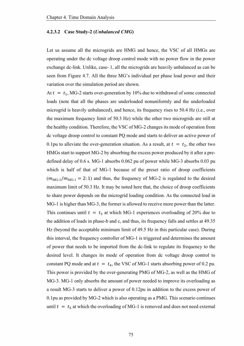
Chapter 4. Time Domain Analysis
75
4.2.3.2 Case Study-2 (Unbalanced CMG)
Let us assume all the microgrids are HMG and hence, the VSC of all HMGs are
operating under the dc voltage droop control mode with no power flow in the power
exchange dc-link. Unlike, case- 1, all the microgrids are heavily unbalanced as can be
seen from Figure 4.7. All the three MG’s individual per phase load power and their
variation over the simulation period are shown.
At 𝑡 = 𝑡1, MG-2 starts over-generation by 10% due to withdrawal of some connected
loads (note that all the phases are underloaded nonuniformly and the underloaded
microgrid is heavily unbalanced), and hence, its frequency rises to 50.4 Hz (i.e., over
the maximum frequency limit of 50.3 Hz) while the other two microgrids are still at
the healthy condition. Therefore, the VSC of MG-2 changes its mode of operation from
dc voltage droop control to constant PQ mode and starts to deliver an active power of
0.1pu to alleviate the over-generation situation. As a result, at 𝑡 = 𝑡2, the other two
HMGs start to support MG-2 by absorbing the excess power produced by it after a pre-
defined delay of 0.6 s. MG-1 absorbs 0.062 pu of power while MG-3 absorbs 0.03 pu
which is half of that of MG-1 because of the preset ratio of droop coefficients
(𝑚MG-3/𝑚MG-1 = 2: 1) and thus, the frequency of MG-2 is regulated to the desired
maximum limit of 50.3 Hz. It may be noted here that, the choice of droop coefficients
to share power depends on the microgrid loading condition. As the connected load in
MG-1 is higher than MG-3, the former is allowed to receive more power than the latter.
This continues until 𝑡 = 𝑡3 at which MG-1 experiences overloading of 20% due to
the addition of loads in phase-b and c, and thus, its frequency falls and settles at 49.35
Hz (beyond the acceptable minimum limit of 49.5 Hz in this particular case). During
this interval, the frequency controller of MG-1 is triggered and determines the amount
of power that needs to be imported from the dc-link to regulate its frequency to the
desired level. It changes its mode of operation from dc voltage droop control to
constant PQ mode and at 𝑡 = 𝑡4, the VSC of MG-1 starts absorbing power of 0.2 pu.
This power is provided by the over-generating PMG of MG-2, as well as the HMG of
MG-3. MG-1 only absorbs the amount of power needed to improve its overloading as
a result MG-3 starts to deliver a power of 0.12pu in addition to the excess power of
0.1pu as provided by MG-2 which is also operating as a PMG. This scenario continues
until 𝑡 = 𝑡5 at which the overloading of MG-1 is removed and does not need external
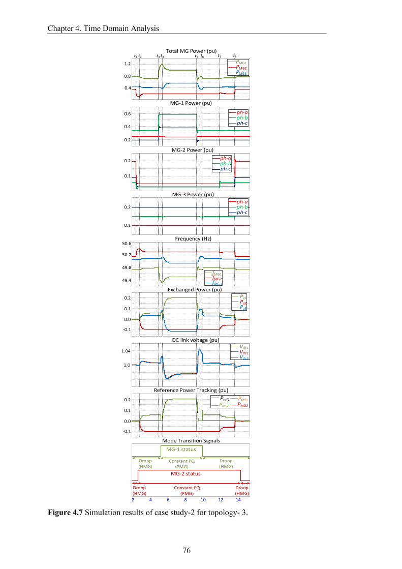
Chapter 4. Time Domain Analysis
76
Total MG Power (pu)
Droop (HMG)
Constant PQ (PMG)
Droop (HMG)
Droop (HMG)
Constant PQ (PMG)
Droop (HMG)
2 4 6 8 10 12 14
MG-2 status
MG-1 status
PMG1
PMG2
PMG3
t1 t2 t3 t4 t5 t6 t7 t8
ph-aph-bph-c
ph-aph-bph-c
ph-aph-bph-c
fMG1fMG2fMG3
Pg1
Pg2
Pg3
Vdc1
Vdc2
Vdc3
PMG1
Pref2 Pref3
PMG2
MG-1 Power (pu)
MG-2 Power (pu)
MG-3 Power (pu)
Frequency (Hz)
Exchanged Power (pu)
DC link voltage (pu)
Reference Power Tracking (pu)
Mode Transition Signals
0.4
0.8
1.2
50.2
49.8
50.6
49.4
0.0
0.1
0.2
-0.1
1.0
1.04
0.0
0.1
0.2
-0.1
0.1
0.2
0.1
0.2
0.2
0.4
0.6
Figure 4.7 Simulation results of case study-2 for topology- 3.

Chapter 4. Time Domain Analysis
77
Table 4.8 Over-generation and overloading events applied to microgrids in case study-
2 at different intervals.
Time
Instant
MG Status Action taken
MG-1 MG-2 MG-3
𝑡1 HMG OG HMG Normal operation for MG-1 and 3 while MG-2 is
over-generating.
𝑡2 HMG PMG HMG MG-2 switches to PQ mode to deliver power and MG-
1 and 3 are operating in droop to support it.
𝑡3 OL PMG HMG MG-1 is over-loaded.
𝑡4 PMG PMG HMG
MG-1 changes its operation mode from droop to PQ to
receive power. Both MG-1 and 2 are supported by
MG-3.
𝑡5 FMG PMG HMG
MG-1’s overload is removed while MG-3 was
supporting MG-2. MG-1 exchanges zero power at this
instant.
𝑡6 HMG PMG HMG MG-1 switches to droop and joins MG-3 in supporting
MG-2.
𝑡7 HMG PMG HMG
MG-2’s over-generation is reduced but still remains
overloaded. The absorbed power by HMGs is
adjusted.
𝑡8 HMG HMG HMG MG-2’s overgeneration is over. All the MGs become
HMG and all MGs switch to droop mode.
support. As a result, the VSC of MG-1 switches its mode of operation from constant
PQ mode to the dc voltage droop control mode with zero power exchange. However,
as the CMG still includes an over-generating PMG (i.e., MG-2), the HMG of MG-3
starts to absorb the excess power of MG-2. At 𝑡 = 𝑡6 MG-1 switches back in dc
droop mode and starts absorbing excess power in addition to MG-3, based on their
preset droop coefficient value as before. At 𝑡 = 𝑡7, some load is added back to phase-
b of MG-2 and hence reduces the excess generation from 10% to 6%. The frequency
controller of MG-2 adjusts the power reference to 0.06pu and thus the power absorbed
by MG-1 and MG-3 are 0.038pu and 0.018pu respectively. At 𝑡 = 𝑡8, the situation of
excess generation in MG-2 is alleviated and goes back to its nominal operating
condition to become an HMG. Thus, the exchange of power is ceased and the VSC of
MG-2 switches back to dc voltage droop. Table 4.8 summarises the events applied to
the microgrids and the corresponding actions taken according to the proposed control
mechanism for study case- 2
4.2.4 Coordinated Control Mechanism among BESs and CMGs
To evaluate the dynamic performance of the proposed coordinated control mechanism
of power-sharing among BESs and CMGs, let us consider the system of Fig. 3.22 with
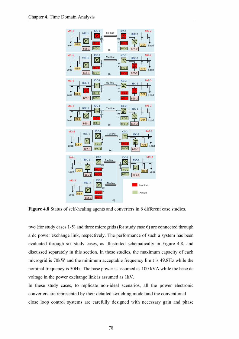
Chapter 4. Time Domain Analysis
78
DER
BES-1
DER
BES-2
Load Load
BSC-2BSC-1ICC-1 ICC-2MG-1 MG-2
DER
BES-1
DER
BES-2
Load Load
BSC-2BSC-1ICC-1 ICC-2MG-1 MG-2
DER
BES-1
DER
BES-2
Load Load
BSC-2BSC-1ICC-1 ICC-2MG-1 MG-2
DER
BES-1
DER
BES-2
Load Load
BSC-2BSC-1ICC-1 ICC-2MG-1 MG-2
(a)
(b)
(c)
(d)
Tie-line
Tie-line
Tie-line
Tie-line
DER
BES-1
DER
BES-2
Load Load
BSC-2BSC-1ICC-1 ICC-2MG-1 MG-2
(e)
Tie-line
Inactive
Active
BFC-1
IFC-2
BFC-2
IFC-1
BFC-1
IFC-1 IFC-2
BFC-2
BFC-1
IFC-1 IFC-2
BFC-2
IFC-2
BFC-2
IFC-1
BFC-1
BFC-1
IFC-1 IFC-2
BFC-2
DER
BES-1
DER
BES-2
Load Load
BSC-2BSC-1ICC-1 ICC-2MG-1 MG-2
(f)
Tie-line
BFC-1
IFC-1 IFC-2
BFC-2
DER
BES-3Load
BSC-3ICC-3MG-3
BFC-3
IFC-3
Tie-line
Figure 4.8 Status of self-healing agents and converters in 6 different case studies.
two (for study cases 1-5) and three microgrids (for study case 6) are connected through
a dc power exchange link, respectively. The performance of such a system has been
evaluated through six study cases, as illustrated schematically in Figure 4.8, and
discussed separately in this section. In these studies, the maximum capacity of each
microgrid is 70kW and the minimum acceptable frequency limit is 49.8Hz while the
nominal frequency is 50Hz. The base power is assumed as 100 kVA while the base dc
voltage in the power exchange link is assumed as 1kV.
In these study cases, to replicate non-ideal scenarios, all the power electronic
converters are represented by their detailed switching model and the conventional
close loop control systems are carefully designed with necessary gain and phase
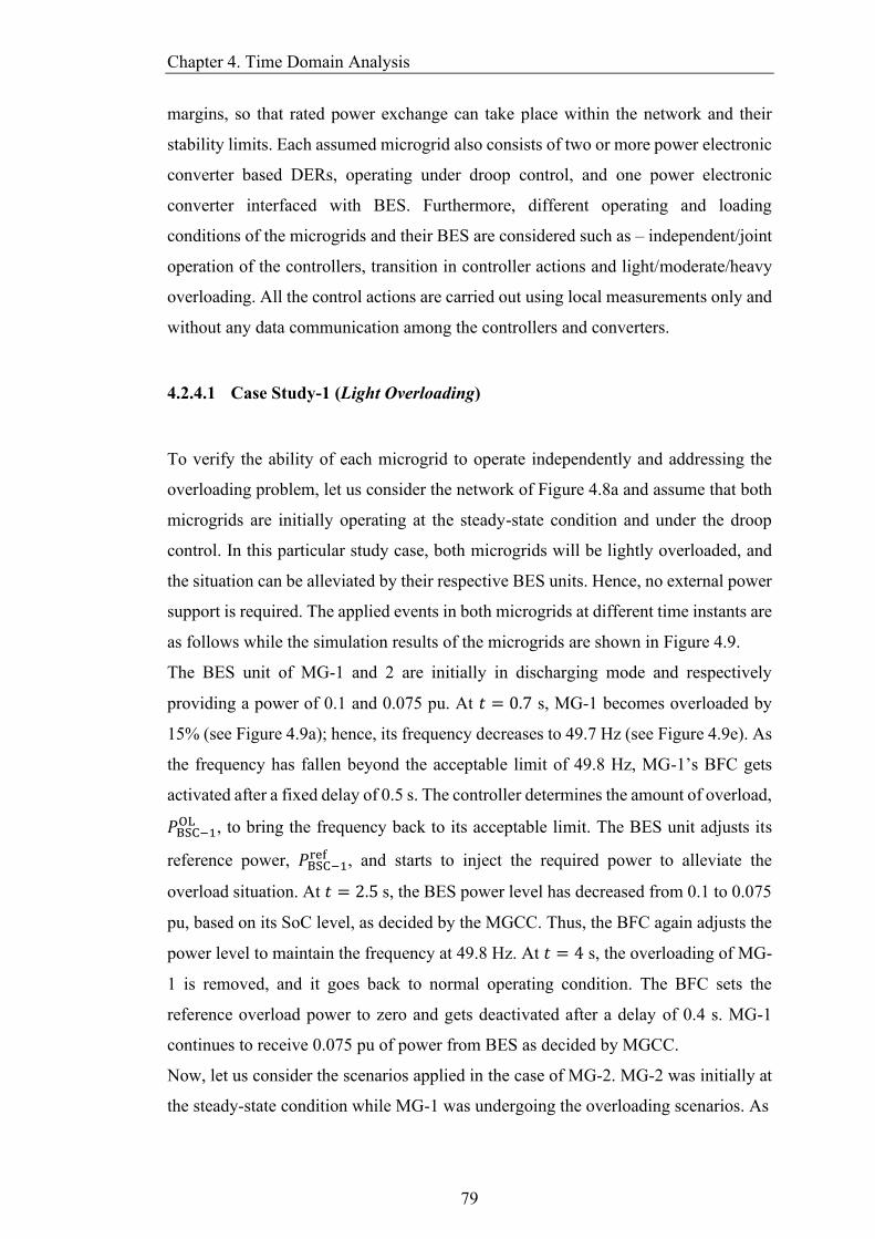
Chapter 4. Time Domain Analysis
79
margins, so that rated power exchange can take place within the network and their
stability limits. Each assumed microgrid also consists of two or more power electronic
converter based DERs, operating under droop control, and one power electronic
converter interfaced with BES. Furthermore, different operating and loading
conditions of the microgrids and their BES are considered such as – independent/joint
operation of the controllers, transition in controller actions and light/moderate/heavy
overloading. All the control actions are carried out using local measurements only and
without any data communication among the controllers and converters.
4.2.4.1 Case Study-1 (Light Overloading)
To verify the ability of each microgrid to operate independently and addressing the
overloading problem, let us consider the network of Figure 4.8a and assume that both
microgrids are initially operating at the steady-state condition and under the droop
control. In this particular study case, both microgrids will be lightly overloaded, and
the situation can be alleviated by their respective BES units. Hence, no external power
support is required. The applied events in both microgrids at different time instants are
as follows while the simulation results of the microgrids are shown in Figure 4.9.
The BES unit of MG-1 and 2 are initially in discharging mode and respectively
providing a power of 0.1 and 0.075 pu. At 𝑡 = 0.7 s, MG-1 becomes overloaded by
15% (see Figure 4.9a); hence, its frequency decreases to 49.7 Hz (see Figure 4.9e). As
the frequency has fallen beyond the acceptable limit of 49.8 Hz, MG-1’s BFC gets
activated after a fixed delay of 0.5 s. The controller determines the amount of overload,
𝑃BSC−1OL , to bring the frequency back to its acceptable limit. The BES unit adjusts its
reference power, 𝑃BSC−1ref , and starts to inject the required power to alleviate the
overload situation. At 𝑡 = 2.5 s, the BES power level has decreased from 0.1 to 0.075
pu, based on its SoC level, as decided by the MGCC. Thus, the BFC again adjusts the
power level to maintain the frequency at 49.8 Hz. At 𝑡 = 4 s, the overloading of MG-
1 is removed, and it goes back to normal operating condition. The BFC sets the
reference overload power to zero and gets deactivated after a delay of 0.4 s. MG-1
continues to receive 0.075 pu of power from BES as decided by MGCC.
Now, let us consider the scenarios applied in the case of MG-2. MG-2 was initially at
the steady-state condition while MG-1 was undergoing the overloading scenarios. As
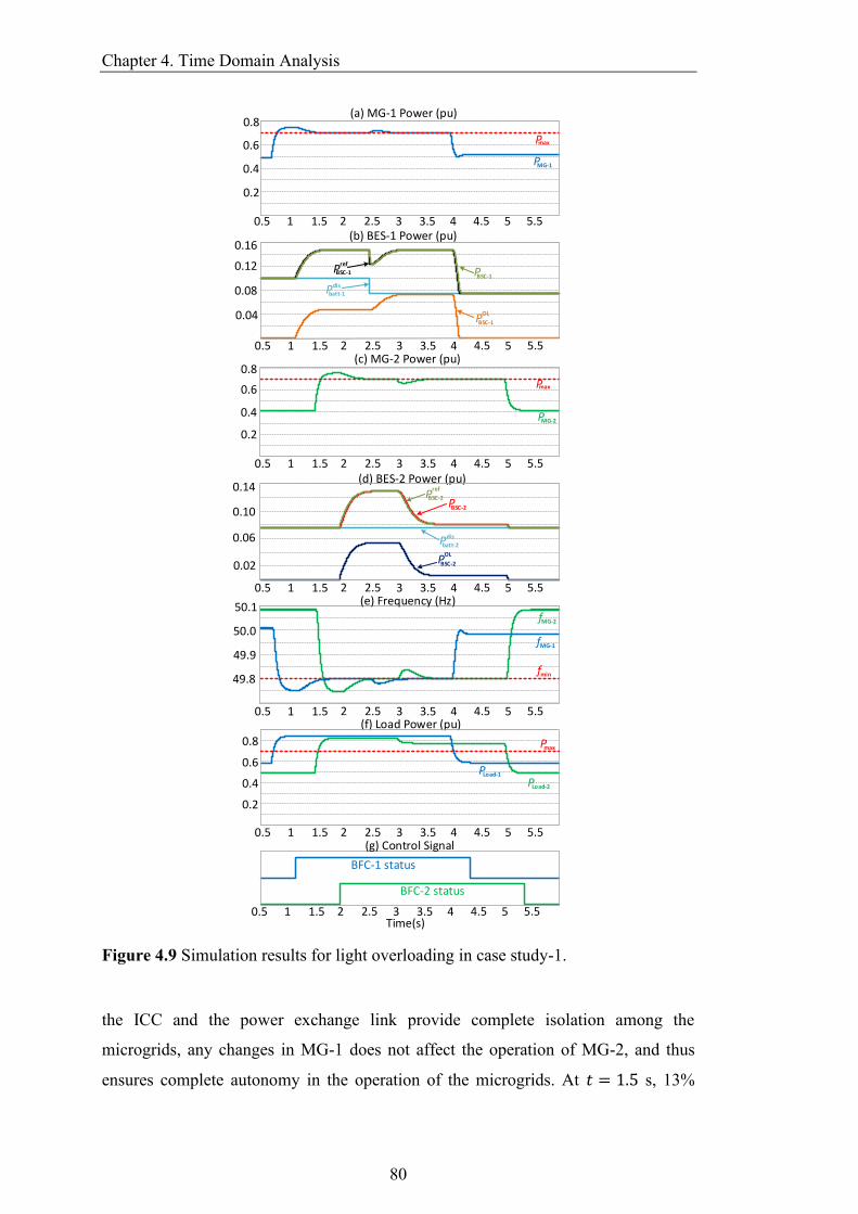
Chapter 4. Time Domain Analysis
80
(a) MG-1 Power (pu)
(b) BES-1 Power (pu)
(c) MG-2 Power (pu)
(d) BES-2 Power (pu)
fMG-2
fMG-1
fmin
(e) Frequency (Hz)
(f) Load Power (pu)
(g) Control Signal
BFC-1 status
BFC-2 status
49.8
49.9
50.0
50.1
0.5 1 2 2.5 3 3.5 4 4.5 5 5.51.5
0.5 1 2 2.5 3 3.5 4 4.5 5 5.51.5
0.5 1 2 2.5 3 3.5 4 4.5 5 5.51.5
0.5 1 2 2.5 3 3.5 4 4.5 5 5.51.5
0.5 1 2 2.5 3 3.5 4 4.5 5 5.51.5
0.5 1 2 2.5 3 3.5 4 4.5 5 5.51.5
0.5 1 2 2.5 3 3.5 4 4.5 5 5.51.5Time(s)
PLoad-2
PLoad-1
Pmax
0.2
0.4
0.6
0.8
Pref
BSC-2PBSC-2
Pbatt-2
dis
PBSC-2
OL
0.02
0.10
0.06
0.14
PMG-1
Pmax
0.2
0.4
0.6
0.8
Pref
BSC-1
Pbatt-1
dis
PBSC-1
PBSC-1
OL0.04
0.12
0.08
0.16
Pmax
PMG-2
0.2
0.4
0.6
0.8
Figure 4.9 Simulation results for light overloading in case study-1.
the ICC and the power exchange link provide complete isolation among the
microgrids, any changes in MG-1 does not affect the operation of MG-2, and thus
ensures complete autonomy in the operation of the microgrids. At 𝑡 = 1.5 s, 13%
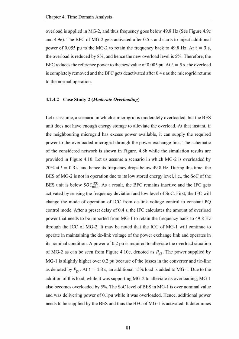
Chapter 4. Time Domain Analysis
81
overload is applied in MG-2, and thus frequency goes below 49.8 Hz (See Figure 4.9c
and 4.9e). The BFC of MG-2 gets activated after 0.5 s and starts to inject additional
power of 0.055 pu to the MG-2 to retain the frequency back to 49.8 Hz. At 𝑡 = 3 s,
the overload is reduced by 8%, and hence the new overload level is 5%. Therefore, the
BFC reduces the reference power to the new value of 0.005 pu. At 𝑡 = 5 s, the overload
is completely removed and the BFC gets deactivated after 0.4 s as the microgrid returns
to the normal operation.
4.2.4.2 Case Study-2 (Moderate Overloading)
Let us assume, a scenario in which a microgrid is moderately overloaded, but the BES
unit does not have enough energy storage to alleviate the overload. At that instant, if
the neighbouring microgrid has excess power available, it can supply the required
power to the overloaded microgrid through the power exchange link. The schematic
of the considered network is shown in Figure. 4.8b while the simulation results are
provided in Figure 4.10. Let us assume a scenario in which MG-2 is overloaded by
20% at 𝑡 = 0.3 s, and hence its frequency drops below 49.8 Hz. During this time, the
BES of MG-2 is not in operation due to its low stored energy level, i.e., the SoC of the
BES unit is below 𝑆𝑂𝐶minICC . As a result, the BFC remains inactive and the IFC gets
activated by sensing the frequency deviation and low level of SoC. First, the IFC will
change the mode of operation of ICC from dc-link voltage control to constant PQ
control mode. After a preset delay of 0.4 s, the IFC calculates the amount of overload
power that needs to be imported from MG-1 to retain the frequency back to 49.8 Hz
through the ICC of MG-2. It may be noted that the ICC of MG-1 will continue to
operate in maintaining the dc-link voltage of the power exchange link and operates in
its nominal condition. A power of 0.2 pu is required to alleviate the overload situation
of MG-2 as can be seen from Figure 4.10c, denoted as 𝑃g2. The power supplied by
MG-1 is slightly higher over 0.2 pu because of the losses in the converter and tie-line
as denoted by 𝑃g1. At 𝑡 = 1.3 s, an additional 15% load is added to MG-1. Due to the
addition of this load, while it was supporting MG-2 to alleviate its overloading, MG-1
also becomes overloaded by 5%. The SoC level of BES in MG-1 is over nominal value
and was delivering power of 0.1pu while it was overloaded. Hence, additional power
needs to be supplied by the BES and thus the BFC of MG-1 is activated. It determines
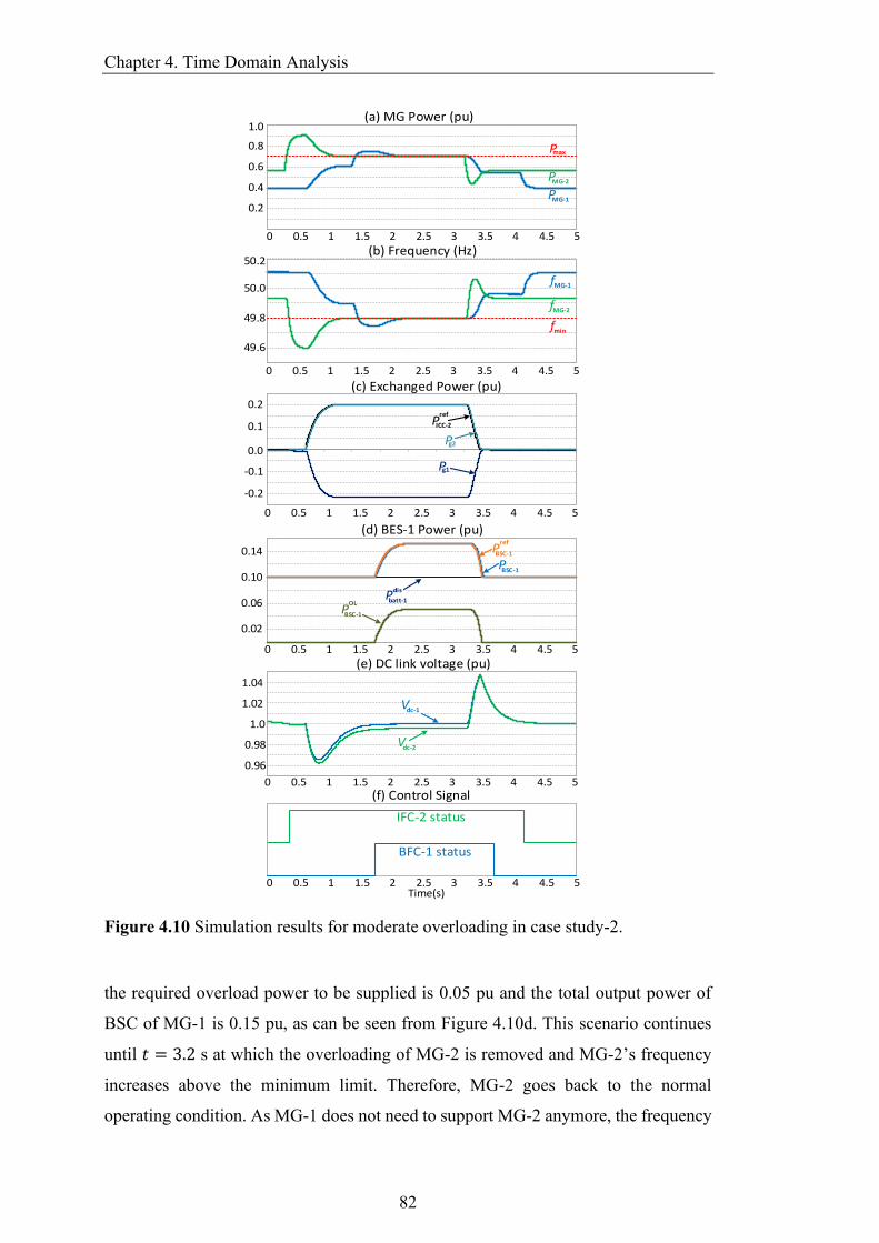
Chapter 4. Time Domain Analysis
82
0 0.5 1 1.5 2 2.5 3 3.5 4 4.5 5
(a) MG Power (pu)
(b) Frequency (Hz)
0 0.5 1 1.5 2 2.5 3 3.5 4 4.5 5
(c) Exchanged Power (pu)
0 0.5 1 1.5 2 2.5 3 3.5 4 4.5 5
(d) BES-1 Power (pu)
0 0.5 1 1.5 2 2.5 3 3.5 4 4.5 5
(e) DC link voltage (pu)
0 0.5 1 1.5 2 2.5 3 3.5 4 4.5 5
0 0.5 1 1.5 2 2.5 3 3.5 4 4.5 5
(f) Control Signal
49.8
49.6
50.0
50.2
0.2
0.4
0.6
0.8
PMG-1
Pmax
fMG-2
fMG-1
fmin
Pref
ICC-2
Pbatt-1
dis
PBSC-1
PBSC-1
OL
PMG-2
Pg2
Pg1
PBSC-1
ref
Vdc-1
Vdc-2
BFC-1 status
IFC-2 status
1.0
0.02
0.1
0.06
0.14
0.0
0.2
-0.1
-0.2
0.10
1.0
1.02
1.04
0.98
0.96
Time(s)
Figure 4.10 Simulation results for moderate overloading in case study-2.
the required overload power to be supplied is 0.05 pu and the total output power of
BSC of MG-1 is 0.15 pu, as can be seen from Figure 4.10d. This scenario continues
until 𝑡 = 3.2 s at which the overloading of MG-2 is removed and MG-2’s frequency
increases above the minimum limit. Therefore, MG-2 goes back to the normal
operating condition. As MG-1 does not need to support MG-2 anymore, the frequency
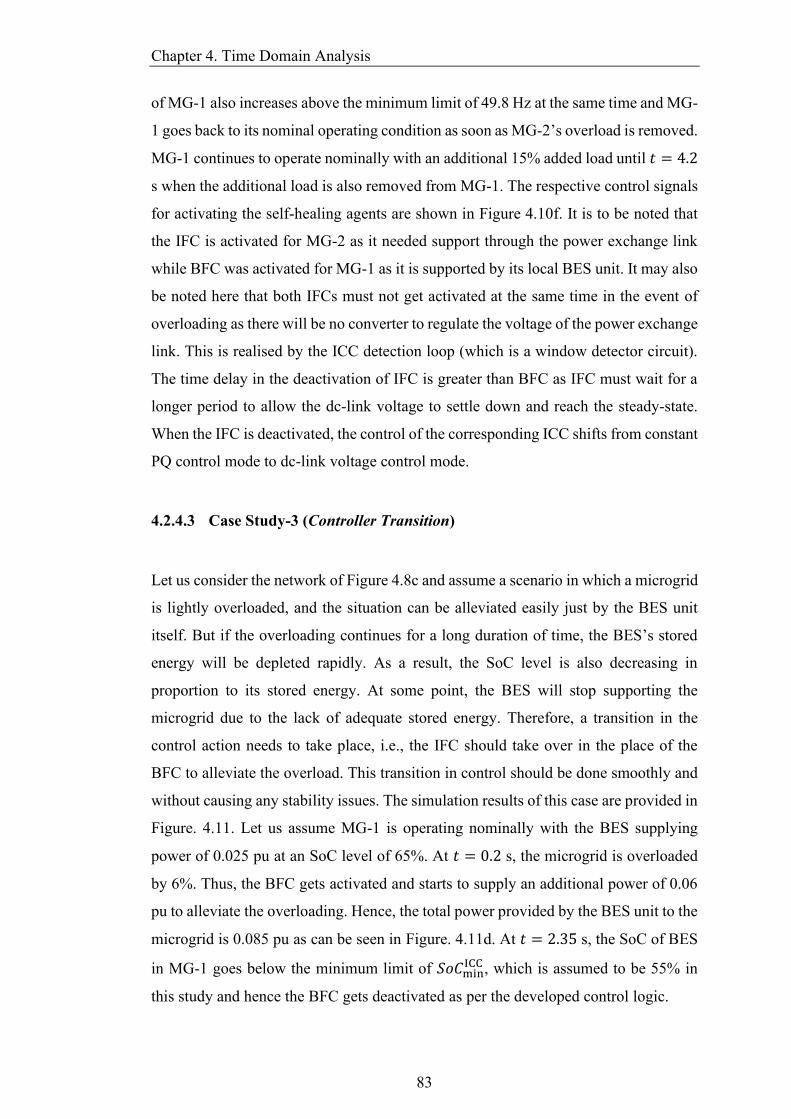
Chapter 4. Time Domain Analysis
83
of MG-1 also increases above the minimum limit of 49.8 Hz at the same time and MG-
1 goes back to its nominal operating condition as soon as MG-2’s overload is removed.
MG-1 continues to operate nominally with an additional 15% added load until 𝑡 = 4.2
s when the additional load is also removed from MG-1. The respective control signals
for activating the self-healing agents are shown in Figure 4.10f. It is to be noted that
the IFC is activated for MG-2 as it needed support through the power exchange link
while BFC was activated for MG-1 as it is supported by its local BES unit. It may also
be noted here that both IFCs must not get activated at the same time in the event of
overloading as there will be no converter to regulate the voltage of the power exchange
link. This is realised by the ICC detection loop (which is a window detector circuit).
The time delay in the deactivation of IFC is greater than BFC as IFC must wait for a
longer period to allow the dc-link voltage to settle down and reach the steady-state.
When the IFC is deactivated, the control of the corresponding ICC shifts from constant
PQ control mode to dc-link voltage control mode.
4.2.4.3 Case Study-3 (Controller Transition)
Let us consider the network of Figure 4.8c and assume a scenario in which a microgrid
is lightly overloaded, and the situation can be alleviated easily just by the BES unit
itself. But if the overloading continues for a long duration of time, the BES’s stored
energy will be depleted rapidly. As a result, the SoC level is also decreasing in
proportion to its stored energy. At some point, the BES will stop supporting the
microgrid due to the lack of adequate stored energy. Therefore, a transition in the
control action needs to take place, i.e., the IFC should take over in the place of the
BFC to alleviate the overload. This transition in control should be done smoothly and
without causing any stability issues. The simulation results of this case are provided in
Figure. 4.11. Let us assume MG-1 is operating nominally with the BES supplying
power of 0.025 pu at an SoC level of 65%. At 𝑡 = 0.2 s, the microgrid is overloaded
by 6%. Thus, the BFC gets activated and starts to supply an additional power of 0.06
pu to alleviate the overloading. Hence, the total power provided by the BES unit to the
microgrid is 0.085 pu as can be seen in Figure. 4.11d. At 𝑡 = 2.35 s, the SoC of BES
in MG-1 goes below the minimum limit of 𝑆𝑜𝐶minICC , which is assumed to be 55% in
this study and hence the BFC gets deactivated as per the developed control logic.
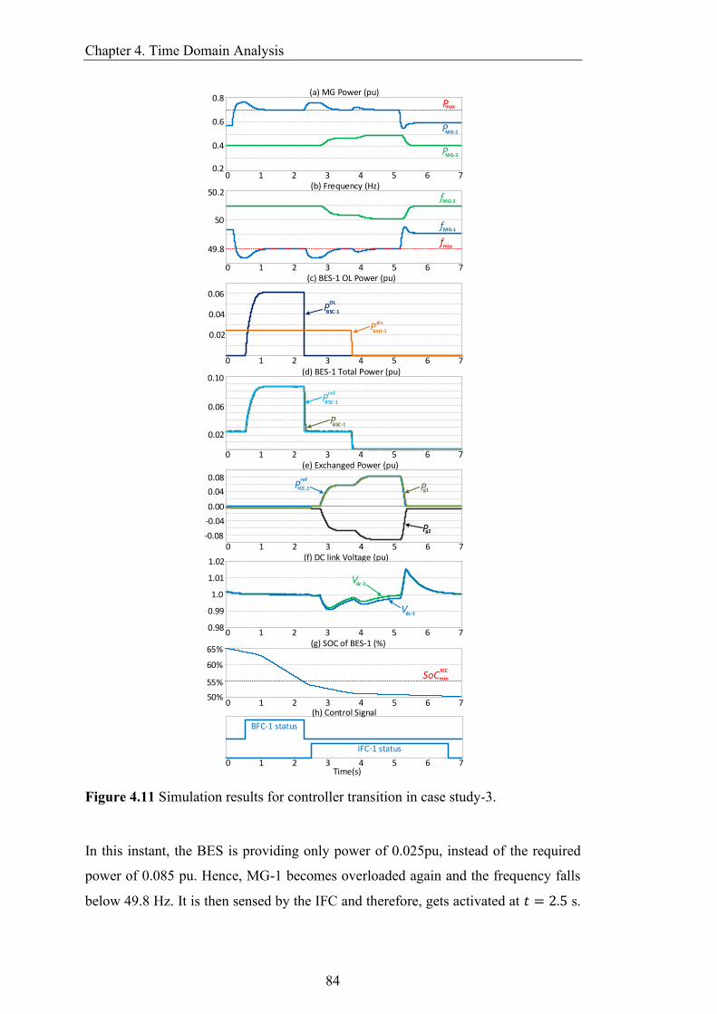
Chapter 4. Time Domain Analysis
84
0 1 2 3 4 5 6 7
(a) MG Power (pu)
(b) Frequency (Hz)
(c) BES-1 OL Power (pu)
(d) BES-1 Total Power (pu)
(e) Exchanged Power (pu)
(f) DC link Voltage (pu)
(g) SOC of BES-1 (%)
(h) Control Signal
Time(s)
PMG-1
Pmax
fMG-2
fMG-1
fmin
PMG-2
Pref
ICC-1
Pg2
Pg1
Pbatt-1
dis
PBSC-1
PBSC-1
OL
PBSC-1
ref
Vdc-1
Vdc-2
SoCICC
min55%
60%
65%
BFC-1 status
IFC-1 status
0.8
0.6
0.4
0.2
49.8
50
50.2
0.02
0.04
0.06
0.02
0.06
0.10
0.04
0.08
0.00
-0.04
-0.08
1.0
1.01
1.02
0.99
0.98
50%
0 1 2 3 4 5 6 7
0 1 2 3 4 5 6 7
0 1 2 3 4 5 6 7
0 1 2 3 4 5 6 7
0 1 2 3 4 5 6 7
0 1 2 3 4 5 6 7
0 1 2 3 4 5 6 7
Figure 4.11 Simulation results for controller transition in case study-3.
In this instant, the BES is providing only power of 0.025pu, instead of the required
power of 0.085 pu. Hence, MG-1 becomes overloaded again and the frequency falls
below 49.8 Hz. It is then sensed by the IFC and therefore, gets activated at 𝑡 = 2.5 s.

Chapter 4. Time Domain Analysis
85
The subsequent steps of operation of IFC are the same as it was in the study case-2.
IFC enables the ICC to import a power of 0.06 pu from MG-2 to alleviate the overload.
This is continued until 𝑡 = 3.8 s at which the BES of MG-1 completely stops supplying
power to MG-1 as decided by the MGCC based on its SoC level. Therefore, the IFC
adjusts the required power demand to retain the frequency back to 49.8 Hz once again.
The overload of MG-1 is removed at 𝑡 = 5.2 s and it goes back to its nominal operation
again. The IFC waits for a certain time for the dc-link voltage to settle and then
switches back to the dc-link voltage control mode.
4.2.4.4 Case Study-4 (Heavy Overloading-1)
To alleviate a heavy overloading situation, the total power may be shared between the
local BES and the neighbouring MG. In the event of any overloading, it is expected
that the microgrid should first try to alleviate the problem using local BES. If the stored
energy of BES or the capacity of the BSC is not enough to address the overload
problem, the microgrid should start importing power through ICC. Both BSC and ICC
should operate simultaneously to supply the overload power demand. Now, let us
consider the network of Figure. 4.8d. Let us assume a scenario where both the
microgrids are operating in nominal condition as can be seen in Figure. 4.12. The SoC
level of both BESs is at the maximum level. Hence both are supplying rated discharge
power of 0.1pu to their respective microgrids. At 𝑡 = 0.2 s, 18% overload has occurred
in MG-2, and as a result, the frequency drops drastically below 49.8 Hz. This situation
is sensed by BFC and it gets activated at 𝑡 = 0.5 s. At 𝑡 = 0.7 s, the BFC starts to
generate the reference power to alleviate the overload situation as can be seen from
Figure. 4.12c. Due to heavy overloading, the required power reference produced by
the PI controller exceeds the maximum rated capacity of BSC, 𝑃BSCmax, which is assumed
as 0.2 pu in this study. Hence, the PI controller should freeze (not reset) by setting its
input to zero using the multiplexer circuit. Thus, the output of the PI controller will
retain the evaluated value which is the maximum power that can be delivered by the
BES unit at that SoC level. This is realised by comparing the instantaneous output
power of BSC, 𝑃BSC, with 𝑃BSCmax. The parameter of 𝑃BSC
max can be dynamically varied
and evaluated based on the SoC level. In this study case, 𝑃BSCmax is set based on the
BSC’s maximum capacity, as BES’s SoC level is at its maximum level. In any other

Chapter 4. Time Domain Analysis
86
90%
100%
80%
(a) MG Power (pu)
0 1 2 3 4 5 6 7 8 9(b) Frequency (Hz)
0 1 2 3 4 5 6 7 8 9(c) BES-2 Power (pu)
0 1 2 3 4 5 6 7 8 9(d) Exchanged Power (pu)
0 1 2 3 4 5 6 7 8 9(e) BES-1 Power (pu)
0 1 2 3 4 5 6 7 8 9
0 1 2 3 4 5 6 7 8 9
(f) DC link Voltage (pu)
(g) SOC Level (%)
0 1 2 3 4 5 6 7 8 9(h) Control Signal
0 1 2 3 4 5 6 7 8 9
PMG-1
Pmax
PMG-2
fMG-2
fMG-1
fmin
Pbatt-2
dis
PBSC-2 PBSC-2
ref
Pref
ICC-2
Pg1
Pg2
PBSC-1
PBSC-1
OL
PBSC-1
ref
Vdc-1
Vdc-2
BES-1
BES-2
BFC-1 status
BFC-2 status
IFC-2 status
0.8
0.6
0.4
0.2
49.8
50
50.2
49.6
0.1
0.2
0.0
0.0
-0.2
0.2
0.1
0.16
0.04
1.0
1.04
1.02
0.98
Time(s)
Figure 4.12 Simulation results for heavy overloading- 1 in case study- 4.
scenario, 𝑃BSCmax can be evaluated dynamically based on the BES’ SoC level. This means
that even though the BSC is capable to handle the required overload power, the SoC
level of the BES is insufficient to produce it. Hence, 𝑃BSCmax needs to be updated
Chapter 4. Time Domain Analysis
87
dynamically based on its SoC level and such freezing mechanism of PI controller is
needed for this purpose. While both BSC and BES reach their maximum power limit
of 0.2 pu, the overloading of the microgrid is not alleviated, and hence, the frequency
still stays below 49.8Hz, as can be seen from Figure. 4.12b and 4.12c. This situation
makes the IFC gets activated at 𝑡 = 1.1 s. The ICC of MG-2 changes its operation
from the dc-link voltage control mode to constant PQ mode and starts importing power
from MG-1 at 𝑡 = 1.5 s. Thus, the overload of the MG-2 is alleviated with both self-
healing agents working simultaneously during which the BSC provides a power of 0.1
pu while the ICC supplies power of 0.12 pu, as can be seen from Figure. 4.12d. Due
to the rapid discharge rate of BES-2 (as it is operating at its maximum capacity due to
overload), at 𝑡 = 3 s, the MGCC reduces the power from 0.1 to 0.05 pu. Therefore,
the IFC increases the ICC’s power reference to maintain the frequency at 49.8 Hz. At
𝑡 = 4.5 s, MG-1 becomes overloaded by 6%. The BFC of MG-1 gets activated and
alleviates the overload situation. At 𝑡 = 7.5 s, the overloading of MG-2 is removed,
and as a result, both microgrids are back to normal operation. It should be noted that
all the four converters of both microgrids (i.e., 2 BSCs and 2 ICCs) were active and
working in conjunction to alleviate the overload situation. The BFCs of both
microgrids were active whereas the IFC of only MG-2 was active (as both IFCs are
not allowed to get activated simultaneously). This is realised by the activated control
signals, as shown in Figure. 4.12h.
4.2.4.5 Case Study-5 (Heavy Overloading-2)
To investigate the efficacy and capability of alleviating the overloading situation in a
decentralised manner, another heavy overloading situation is considered. This study
verifies that a lightly or moderately overloaded microgrid which is being supported by
its BES can support its heavily overloaded neighbouring microgrid through
interconnection. The proposed decentralised topology will enable the microgrids to
exchange power among themselves during overload situation as long as at least one
IFC is inactive. In other words, as long as a microgrid exists that is capable of
regulating the voltage of the power exchange link, the exchange of power among them
can take place, even though that particular microgrid may be overloaded and being
supported by its BES unit. Consider the network of Figure. 4.8e for this study while
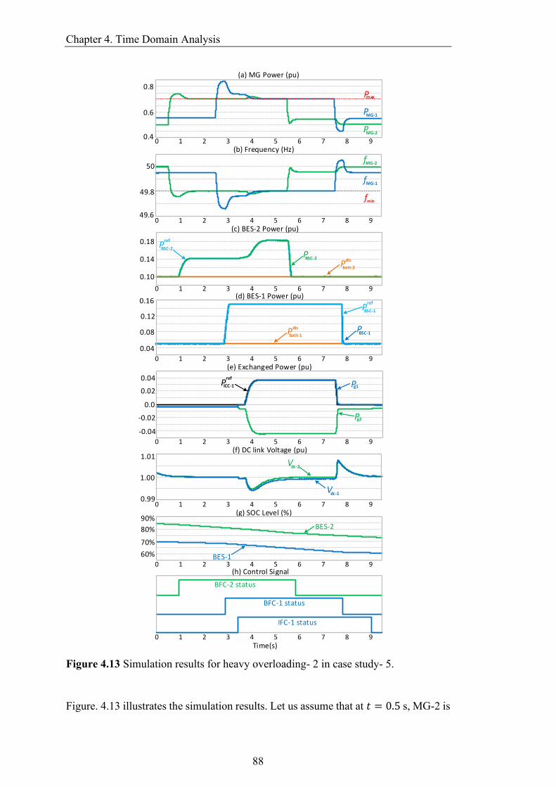
Chapter 4. Time Domain Analysis
88
0 1 2 3 4 5 6 7 8 9
(a) MG Power (pu)
0 1 2 3 4 5 6 7 8 9
(b) Frequency (Hz)
0 1 2 3 4 5 6 7 8 9
(c) BES-2 Power (pu)
(d) BES-1 Power (pu)
0 1 2 3 4 5 6 7 8 9(e) Exchanged Power (pu)
0 1 2 3 4 5 6 7 8 9(f) DC link Voltage (pu)
0 1 2 3 4 5 6 7 8 9(g) SOC Level (%)
0 1 2 3 4 5 6 7 8 9(h) Control Signal
0 1 2 3 4 5 6 7 8 9Time(s)
0.8
0.6
0.4
49.8
50
49.6
0.10
0.18
0.14
0.04
0.08
0.12
0.16
0.04
0.0
-0.02
0.02
-0.04
1.00
1.01
0.99
70%
80%
90%
60%
PMG-1
Pmax
PMG-2
fMG-2
fMG-1
fmin
Pbatt-2
disPBSC-2
PBSC-2
ref
Pbatt-1
dis PBSC-1
PBSC-1
ref
Pg2
Pg1Pref
ICC-1
Vdc-2
Vdc-1
BES-2
BES-1
BFC-2 status
BFC-1 status
IFC-1 status
Figure 4.13 Simulation results for heavy overloading- 2 in case study- 5.
Figure. 4.13 illustrates the simulation results. Let us assume that at 𝑡 = 0.5 s, MG-2 is

Chapter 4. Time Domain Analysis
89
overloaded by 5%. As a result, the frequency has dropped below 49.8 Hz. BES-2 was
supplying power of 0.1pu as decided by the MGCC, at the time of overloading. The
drop in frequency level activates the BFC and it adjusts the active power reference for
BSC to supply the required overload power to MG-2. Thus, the frequency returns to
49.8 Hz. The situation continues until 𝑡 = 2.5s at which MG-1 becomes overloaded
by 14%. At the time of overloading, BES-1 was delivering power of 0.05 pu to the
MG. This activates the BFC’s associated controller. The SoC of BES-1 is less than
70% at this time as can be seen from Figure. 4.13g, which sets the maximum power
that is supplied by BSC, 𝑃BSCmax, as 0.15 pu. In this case, the value of 𝑃BSC
max is determined
based on the BES’ SoC value unlike the previous case, where it was chosen based on
the converter’s maximum rating. Due to heavy overloading, the output of the PI
controller of the BFC will reach its maximum limit of 0.15 pu within a short period of
time and freezes, as can be seen from Figure. 4.13d. As the overloading problem is not
alleviated, the IFC of MG-1 will get activated at 𝑡 = 3.4 s. Hence, the mode of
operation of the ICC of MG-1 changes from the dc-link voltage control to the constant
PQ mode. This is a scenario where both microgrids are overloaded (MG-2 is lightly,
and MG-1 is heavily overloaded). As the ICC of MG-1 is changed to constant PQ
mode, the ICC of MG-2 must remain in the dc-link voltage control mode to regulate
the voltage of the power exchange link. It is to be noted that, for a network where more
than two microgrids are interconnected to share power, at least one microgrid is needed
which is not heavily overloaded and can assign its ICC to regulate the dc-link voltage
of the power exchange link. Once, the IFC of MG-1 is activated, it will produce the
desired reference to start importing power from MG-2, as can be seen from Figure.
4.13e. As such, the frequency of MG-1 retains back to 49.8 Hz and the overloading is
alleviated. At 𝑡 = 5.5 s, the overloading in MG-2 is removed and it goes back to its
normal operation mode. However, MG-2 keeps on supporting MG-1, as long as it
remains overloaded. At 𝑡 = 7.5 s, the overloading in MG-1 is removed and it also
moves back to its normal operation. The corresponding activation control signals for
BFCs and IFC of both microgrids are shown in Figure. 4.13h.
4.2.4.6 Case Study- 6 (Multiple MGs)
This study case demonstrates the power-sharing amongst multiple microgrids to

Chapter 4. Time Domain Analysis
90
PMG-2
fmin
0 1 2 3 4 5 6
0 1 2 3 4 5 6
0 1 2 3 4 5 6
(a) MG Power (pu)
(b) Frequency (Hz)
(c) BES-2 Power (pu)
0 1 2 3 4 5 6
(d) Exchanged Power (pu)
(e) DC link Voltage (pu)
0 1 2 3 4 5 6
(f) Control Signal
0 1 2 3 4 5 6
Pmax
PMG-1
PMG-3
fMG-2
fMG-1 fMG-3
PBSC-2
PBSC-2
ref
Pref
ICC-1Pg2
Pg3
Pg1
Vdc-2 Vdc-3
Vdc-1
BFC-2 status
IFC-2 status
0.8
0.6
0.4
1.0
49.8
50.0
49.6
50.2
0.080.04
0.160.12
0.10
0.00
-0.10
1.00
0.98
1.02
0.96
Figure 4.14 Simulation results for Multiple microgrids in case study- 6.
alleviate the overloading situation. Let us consider the network in Figure. 4.8f and
assume a scenario in which three microgrids are coupled through the power exchange
link. The results of this study are provided in Figure. 4.14. Let us assume that all of
the three microgrids are operating in their nominal condition. BES-1, 2 and 3 are
supplying respectively a power of 0.1, 0.05 and 0.1 pu to their respective microgrids,
as can be seen from Figure. 4.14c. At 𝑡 = 0.3 s, MG-2 is overloaded by 22%, and as a
result, the frequency drops below 49.8 Hz. This activates the controller of BFC-2 at
𝑡 = 0.6 s. Based on the SoC level of BES-2, the maximum power that is supplied,
Chapter 4. Time Domain Analysis
91
𝑃𝐵𝑆𝐶𝑚𝑎𝑥, is evaluated as 0.15 pu. As soon as the output power of BSC-2 reaches 0.15 pu,
the controller of BFC-2 freezes, as can be seen from Figure. 4.14c. As the frequency
of MG-2 is still below 49.8 Hz, IFC-2 will get activated at 𝑡 = 1.2 s, and hence, the
mode of operation of ICC-2 changes from the dc-link voltage control to constant PQ
mode. At 𝑡 = 1.5 s, both MG-1and MG-3 start supplying power to MG-2 to alleviate
the overloading situation with a power ratio of 𝑃𝑔1: 𝑃𝑔3 = 2: 1, as determined by their
droop coefficients. It is expected that the power shared by MG-1 should be greater
than MG-3 as the loading of MG-1 is less than MG-3 (See Figure. 4.14a). The total
overload power demand for MG-2 is 0.1245 pu where the supplied power from MG-1
and MG-3 are respectively 0.091 and 0.0458 pu, as can be seen from Figure. 4.14d.
To obtain the desired power-sharing, the ratio of droop coefficients of MG-3 and MG-
1 is set as 𝑞𝑀𝐺−3: 𝑞𝑀𝐺−1 = 2: 1 based on the ratio of their droop coefficients. The
excess power supplied by MG-1 and MG-3, in addition to the overload power of MG-
2, is to overcome the line and converter losses. At 𝑡 = 4 s, the overloading of MG-2
is removed, and it goes back to its normal operation, and as such, both MG-1 and MG-
3 cease to supply power to it. The corresponding control activation signals for BFC-2
and IFC-2 are shown in Figure. 4.14f.
4.3 Comparison in performance of the three topologies
Based on the time domain case studies, comparative performance analysis can be done
for all of the three topologies. First, a comparison based on the output power and
voltage quality can be done for topology- 1 and 2. It can be seen that both ac topologies
can successfully alleviate the overloading or over-generation problems based on the
developed control mechanism, however, the power quality is poorer in topology-2 as
single-phase instantaneous power is oscillatory in nature. As a result, the dc-link
voltage in the back-to-back converter contains a larger ripple in the case of topology-
2 as compared to topology- 1. Though the number of components and power lines
require for the three-phase link are more, the power quality and performance are
superior and produce significantly lower line loss and thus, makes the system more
efficient. Hence, the three-phase power exchange link is superior in terms of power
and voltage quality as compared to the single-phase link unless a very small amount
of power is required to be exchanged within the CMG network through short
Chapter 4. Time Domain Analysis
92
interconnecting lines. Moreover, single-phase VSC operating in PQ control mode
requires a phase-shifting for dq transformation that somewhat restricts its operating
frequency range as the phase shifting filter is operational in one particular frequency
(e.g., 50Hz in this case). The employed angle droop control technique is also beneficial
for this purpose as the frequency of operation remains fixed. However, if a frequency
droop control is used instead of angle droop, the performance of the single-phase VSC
will deteriorate in PQ control mode as the power exchange link does not operate at a
fixed frequency value in this case. Three-phase VSCs of topology- 1 does not have
this problem and can be functional in both angle and frequency droop.
It has been already discussed in section 3.2.1.2 how the problem of synchronization
can be overcome in ac interlinking topologies by employing angle droop instead of
frequency droop. However, the dc interconnecting link in topology- 3, does not have
this problem. This feature can be explained by referring to the time domain simulation
results of the case studies of the three topologies. In the dc interconnecting link of
topology-3, once a microgrid becomes an HMG from PMG, it can instantly join the
other HMGs to support the PMGs within a CMG network, unlike topology-1 and 2.
This can be observed from Figure 4.6 and 4.7. At, 𝑡 = 𝑡5 the microgrid’s overloading
is over, it becomes an FMG from a PMG. Thus, after the preset delay of 0.6s at, 𝑡 =
𝑡6 it becomes an HMG and instantly it joins the other HMG to support the PMG.
Whereas, a similar scenario can be noticed at time 𝑡 = 𝑡6 in Figure 4.2 for topology-
1 and Figure 4.5 for topology-2, respectively. In both topologies, though microgrid-1
becomes an HMG at this instant, it cannot get connected back to the other HMGs as
long as there is an operational PMG in the CMG network. Therefore, the newly
recovered HMG must wait until all the PMG(s) become HMG(s) and the exchange of
power among the microgrids in the CMG network ceases completely as the
synchronization with the interconnecting lines is not possible while the other
microgrids are exchanging power. When there is no exchange of power, all the
microgrids are at no load and the power exchange lines will operate at the same phase
angle and voltage magnitude. Hence, at this situation, the mode of operation can be
changed from constant PQ to angle droop control without causing any unwanted power
surge or oscillation within the CMG. This can be seen from Figure 4.2 and Figure 4.5,
at time instant 𝑡 = 𝑡8 when both the microgrids change their mode of operation from
PQ to droop control simultaneously.

Chapter 4. Time Domain Analysis
93
4.4 Summary
This chapter has demonstrated the efficacy of the proposed control technique through
time-domain simulation studies, in retaining the desired upper and lower frequency
limits in autonomous microgrids coupled to a common power exchange link. Such
frequency regulation is achieved through proper exchange of power via the
interconnecting link where the interconnecting link can be made of three different
topologies. Also, it shows a control mechanism to coordinate the power-sharing among
the local BES and the neighbouring microgrids in several scenarios. The presented
case studies in this chapter assume different scenario and critical operating conditions
of the microgrids. The studies also demonstrate that the developed control mechanism
can successfully and effectively alleviate all the overloading and overgeneration
scenarios through proper MG’s frequency regulation and exchange of power without
any communication among the microgrids.
Chapter 5. Stability Analysis
94
Chapter 5 Stability Analysis
This chapter presents the small signal stability analysis of the three proposed power
exchange topologies to determine the stability of the system against different
operational and network parameters. The study reveals the system stability limits and
margins at different operating conditions and its findings help us in selecting the
suitable network and design parameters for different topologies to avoid instability.
5.1. Stability Analysis
The stability of the power exchange strategy for all three CMG topologies is evaluated.
The small signal stability analysis is performed by varying numerous key design
parameters such as the active and reactive power droop coefficients, interconnecting
line’s impedance, and PMG’s power demand. The eigenvalue plots obtained from the
stability analysis are shown in Figure 5.1-5.11.
Among all these parameters, the active power droop coefficient, 𝑚MG, (for topology-
1 and 2) exhibits the most dominating effect over the CMG stability and can drive the
system towards instability; whereas the CMG’s dynamics and response are affected by
the other parameters but have relatively less influence on the system’s stability. For
topology-3, parametric variations affect the network dynamics, but it is not as
dominant as it is in topology-1 and 2 and more importantly, do not lead the system to
instability.
5.1.1. Variation of Droop Coefficients
The active power droop coefficient of 𝑚MG is changed in steps from its nominal value
of 0.002rad/kW for both topology-1 and 2, while the reactive power droop coefficient
of 𝑛MG is kept constant. The coefficient 𝑚MG and 𝑛MG are defined in Equation 3.12
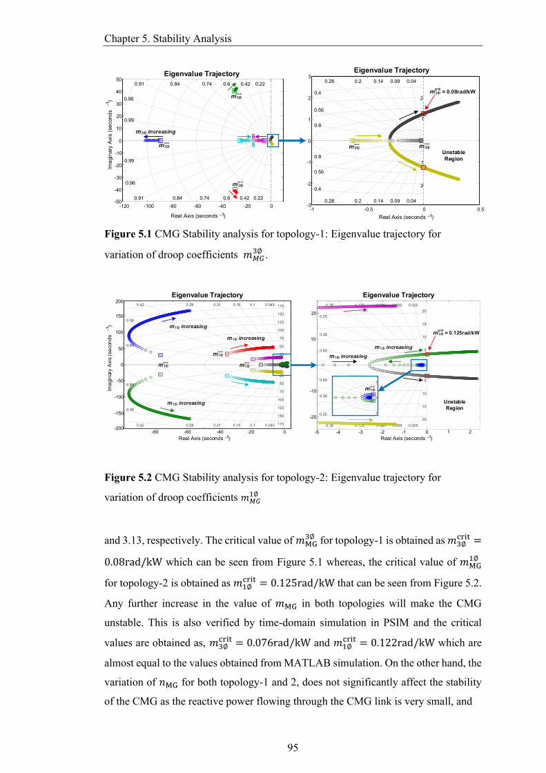
Chapter 5. Stability Analysis
95
-120 -100 -80 -60 -40 -20 0-50
-40
-30
-20
-10
0
10
20
30
40
50
0.22
0.22
0.42
0.420.6
0.6
0.74
0.740.84
0.840.91
0.91
0.96
0.99
0.99
0.96
-1 -0.5 0 0.5-3
-2
-1
0
1
2
3
2
1
2
1
0.04
0.040.09
0.090.14
0.14
0.2
0.2
0.28
0.28
0.56
0.56
0.4
0.4
0.8
0.8
lma
gin
ary
Axis
(se
con
ds
)-1
Unstable
Region
Eigenvalue TrajectoryEigenvalue Trajectory
Real Axis (seconds -1)
m3Φ increasing
no m
m3Φ
no m
m3Φ
no m
m3Φ no m
m3Φ no m
m3Φ
m3Φ = 0.08rad/kWcrit
Real Axis (seconds -1)
Figure 5.1 CMG Stability analysis for topology-1: Eigenvalue trajectory for
variation of droop coefficients 𝑚𝑀𝐺3∅ .
Unstable
Region
m1Φ = 0.125rad/kWcrit
no m
m1Φ
no m
m1Φ
no m
m1Φ
m1Φ increasing
m1Φ increasing
m1Φ increasing
m1Φ increasing
m1Φ increasing
no m
m1Φ
Eigenvalue Trajectory
Real Axis (seconds -1)
Eigenvalue Trajectory
lma
gin
ary
Axis
(se
con
ds
)-1
-80
0
20
100
200
150
-100
-200
-150
-60 -40
-20
0
10
-10
-20 0-1-2-3-4-5 1 2
Real Axis (seconds -1)
-50
50
Figure 5.2 CMG Stability analysis for topology-2: Eigenvalue trajectory for
variation of droop coefficients 𝑚𝑀𝐺1∅
and 3.13, respectively. The critical value of 𝑚MG3∅ for topology-1 is obtained as 𝑚3∅
crit =
0.08rad/kW which can be seen from Figure 5.1 whereas, the critical value of 𝑚MG1∅
for topology-2 is obtained as 𝑚1∅crit = 0.125rad/kW that can be seen from Figure 5.2.
Any further increase in the value of 𝑚MG in both topologies will make the CMG
unstable. This is also verified by time-domain simulation in PSIM and the critical
values are obtained as, 𝑚3∅crit = 0.076rad/kW and 𝑚1∅
crit = 0.122rad/kW which are
almost equal to the values obtained from MATLAB simulation. On the other hand, the
variation of 𝑛MG for both topology-1 and 2, does not significantly affect the stability
of the CMG as the reactive power flowing through the CMG link is very small, and

Chapter 5. Stability Analysis
96
-40 -35 -30 -25 -20 -15 -10 -5 0-60
-40
-20
0
20
40
600.06
0.06
0.12
0.12
0.19
0.19
0.27
0.270.36
0.360.5
0.5
0.88
0.66
0.88
0.66
-12 -10 -8 -6 -4 -2 0
-15
-10
-5
0
5
10
15
0.05
0.050.11
0.11
0.17
0.170.24
0.240.34
0.34
0.46
0.46
0.84
0.62
0.84
0.62
-0.4 -0.35 -0.3 -0.25 -0.2
0
Eigenvalue Trajectory Eigenvalue Trajectory
Real Axis (seconds -1) Real Axis (seconds -1)
lma
gin
ary
Axis
(se
con
ds
)-1
no m
n3Φ
no m
n3Φ
no m
n3Φ
no m
n3Φ
n3Φ increasing
n3Φ increasing
n3Φ increasing
n3Φ increasing
Figure 5.3 CMG Stability analysis for topology-1: Eigenvalue trajectory for
variation of droop coefficients 𝑛𝑀𝐺3∅ .
-60 -50 -40 -30 -20 -10 0-5
-4
-3
-2
-1
0
1
2
3
4
50.7
0.7
0.91
0.91
0.96
0.96
0.98
0.980.99
0.990.996
0.996
0.998
0.998
1
1
-1.5 -1 -0.5 0-1
-0.8
-0.6
-0.4
-0.2
0
0.2
0.4
0.6
0.8
10.12
0.120.26
0.26
0.4
0.40.52
0.52
0.66
0.66
0.8
0.8
0.97
0.97
0.9
0.9
Eigenvalue Trajectory Eigenvalue Trajectory
lma
gin
ary
Axis
(se
con
ds
)-1
Real Axis (seconds -1) Real Axis (seconds -1)
no m
n1Φ
n1Φ increasingn1Φ increasing
n1Φ increasing
n1Φ increasingno m
n1Φ
no m
n1Φ
n1Φ increasing
Figure 5.4 CMG Stability analysis for topology-2: Eigenvalue trajectory for
variation of droop coefficients 𝑛𝑀𝐺1∅ .
hence the variation of 𝑛MG does not have a noticeable effect on the system stability, as
seen from Figure 5.3 and Figure 5.4, respectively. The value of 𝑛MG was varied from
its nominal value of 0.004rad/kVAR up to 0.4rad/kVAR (i.e.,100 times of its nominal
value) to obtain the eigenvalue trajectory plots.
At the nominal value of droop coefficients 𝑚MGnom and 𝑛MG
nom, the response of topology-
2 is more oscillatory (less damping) compare to the topology-1 which can also be
justified from the eigenvalue location for nominal values of droop coefficients as
shown in Figure 5.1-5.4 and also from the frequency response plots of Figure 3.10 and
Figure 3.18. However, topology-1 is more sensitive to variation of droop coefficients
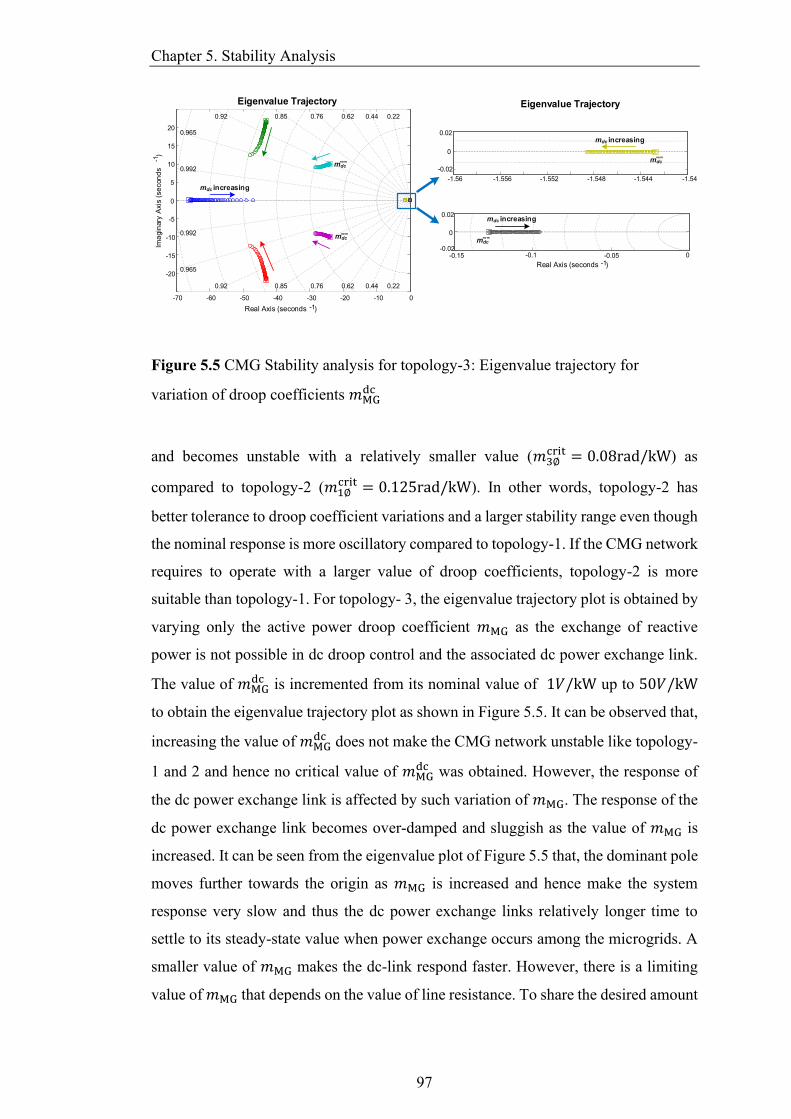
Chapter 5. Stability Analysis
97
Eigenvalue Trajectory
-70 -60 -50 -40 -30 -20 -10 0
-20
-15
-10
-5
0
5
10
15
20
0.22
0.22
0.44
0.440.62
0.620.76
0.76
0.85
0.850.92
0.92
0.992
0.965
0.992
0.965
-1.56 -1.556 -1.552 -1.548 -1.544 -1.54
-0.02
0
0.02
-0.15 -0.1 -0.05 0-0.02
0
0.02
lma
gin
ary
Axis
(se
con
ds
)-1
Real Axis (seconds -1)
Real Axis (seconds -1)
mdc increasing
mdc increasing
mdc increasing
no m
mdc
no m
mdc
no m
mdc
no m
mdc
Eigenvalue Trajectory
Figure 5.5 CMG Stability analysis for topology-3: Eigenvalue trajectory for
variation of droop coefficients 𝑚MGdc
and becomes unstable with a relatively smaller value (𝑚3∅crit = 0.08rad/kW) as
compared to topology-2 (𝑚1∅crit = 0.125rad/kW). In other words, topology-2 has
better tolerance to droop coefficient variations and a larger stability range even though
the nominal response is more oscillatory compared to topology-1. If the CMG network
requires to operate with a larger value of droop coefficients, topology-2 is more
suitable than topology-1. For topology- 3, the eigenvalue trajectory plot is obtained by
varying only the active power droop coefficient 𝑚MG as the exchange of reactive
power is not possible in dc droop control and the associated dc power exchange link.
The value of 𝑚MGdc is incremented from its nominal value of 1𝑉/kW up to 50𝑉/kW
to obtain the eigenvalue trajectory plot as shown in Figure 5.5. It can be observed that,
increasing the value of 𝑚MGdc does not make the CMG network unstable like topology-
1 and 2 and hence no critical value of 𝑚MGdc was obtained. However, the response of
the dc power exchange link is affected by such variation of 𝑚MG. The response of the
dc power exchange link becomes over-damped and sluggish as the value of 𝑚MG is
increased. It can be seen from the eigenvalue plot of Figure 5.5 that, the dominant pole
moves further towards the origin as 𝑚MG is increased and hence make the system
response very slow and thus the dc power exchange links relatively longer time to
settle to its steady-state value when power exchange occurs among the microgrids. A
smaller value of 𝑚MG makes the dc-link respond faster. However, there is a limiting
value of 𝑚MG that depends on the value of line resistance. To share the desired amount
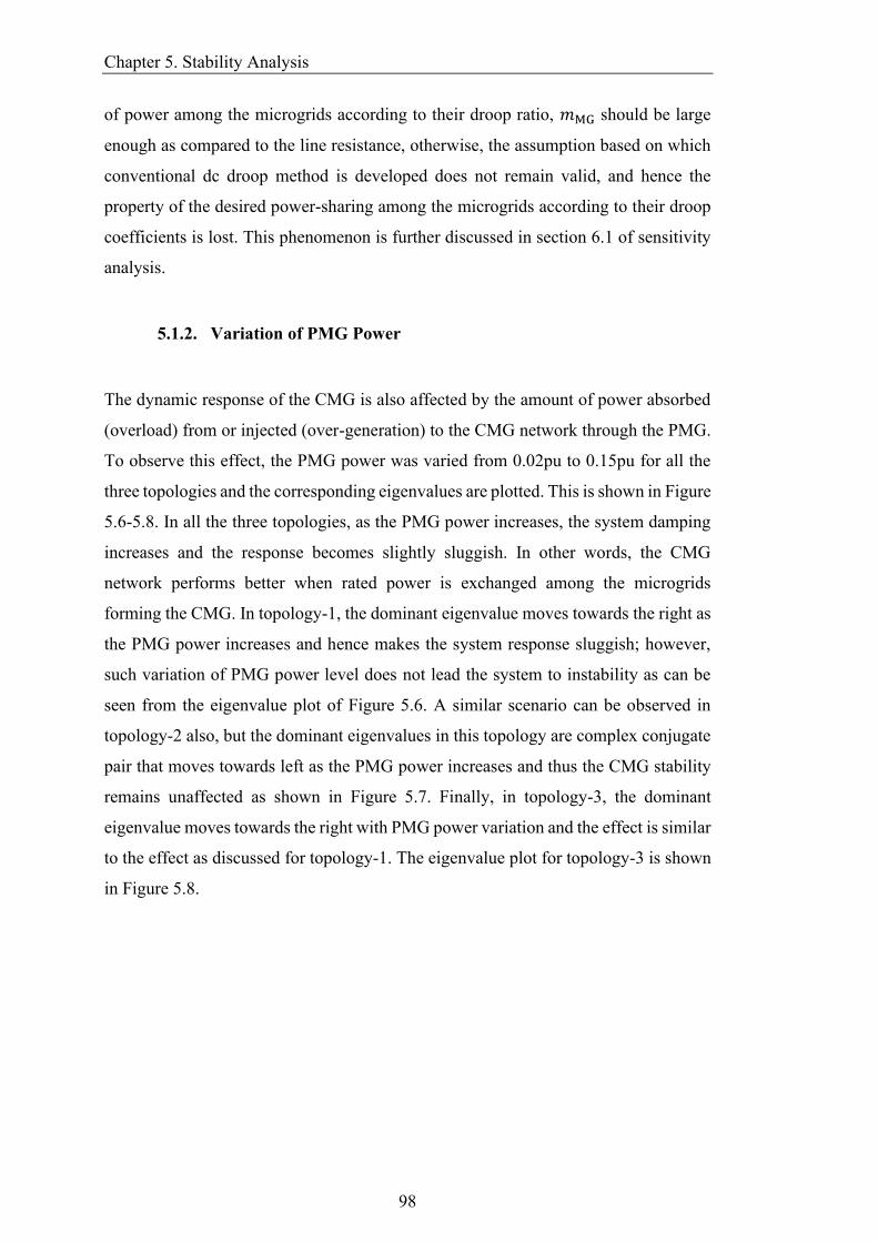
Chapter 5. Stability Analysis
98
of power among the microgrids according to their droop ratio, 𝑚MG should be large
enough as compared to the line resistance, otherwise, the assumption based on which
conventional dc droop method is developed does not remain valid, and hence the
property of the desired power-sharing among the microgrids according to their droop
coefficients is lost. This phenomenon is further discussed in section 6.1 of sensitivity
analysis.
5.1.2. Variation of PMG Power
The dynamic response of the CMG is also affected by the amount of power absorbed
(overload) from or injected (over-generation) to the CMG network through the PMG.
To observe this effect, the PMG power was varied from 0.02pu to 0.15pu for all the
three topologies and the corresponding eigenvalues are plotted. This is shown in Figure
5.6-5.8. In all the three topologies, as the PMG power increases, the system damping
increases and the response becomes slightly sluggish. In other words, the CMG
network performs better when rated power is exchanged among the microgrids
forming the CMG. In topology-1, the dominant eigenvalue moves towards the right as
the PMG power increases and hence makes the system response sluggish; however,
such variation of PMG power level does not lead the system to instability as can be
seen from the eigenvalue plot of Figure 5.6. A similar scenario can be observed in
topology-2 also, but the dominant eigenvalues in this topology are complex conjugate
pair that moves towards left as the PMG power increases and thus the CMG stability
remains unaffected as shown in Figure 5.7. Finally, in topology-3, the dominant
eigenvalue moves towards the right with PMG power variation and the effect is similar
to the effect as discussed for topology-1. The eigenvalue plot for topology-3 is shown
in Figure 5.8.
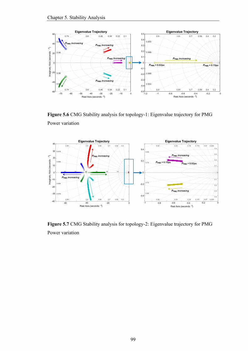
Chapter 5. Stability Analysis
99
-70 -60 -50 -40 -30 -20 -10 0-60
-40
-20
0
20
40
600.1
0.10.22
0.220.34
0.340.46
0.46
0.6
0.60.74
0.74
0.86
0.96
0.96
0.86
-1.2 -1 -0.8 -0.6 -0.4 -0.2 0-0.5
-0.4
-0.3
-0.2
-0.1
0
0.1
0.2
0.3
0.4
0.5
0.2
0.20.4
0.40.56
0.56
0.7
0.70.81
0.81
0.9
0.9
0.955
0.988
0.955
0.988
Real Axis (seconds -1)
lma
gin
ary
Axis
(se
con
ds
)-1
Eigenvalue Trajectory Eigenvalue Trajectory
PPMG increasingPPMG increasing
PPMG increasing
PPMG increasing
PPMG = 0.02pu PPMG = 0.15pu
PPMG increasing
Real Axis (seconds -1)
Figure 5.6 CMG Stability analysis for topology-1: Eigenvalue trajectory for PMG
Power variation
Eigenvalue Trajectory Eigenvalue Trajectory
-60 -40 -20 0
0
10
20
30
lma
gin
ary
Axis
(se
con
ds
)-1
40
-40
-30
-20
-10
-0.4
-0.2
0
0.2
0.4
-0.8 -0.6 -0.4 -0.2 0
Real Axis (seconds -1)
-1
Real Axis (seconds -1)
PPMG increasing
PPMG = 0.02pu
PPMG increasing
PPMG increasing PPMG increasing
PPMG = 0.15pu
Figure 5.7 CMG Stability analysis for topology-2: Eigenvalue trajectory for PMG
Power variation
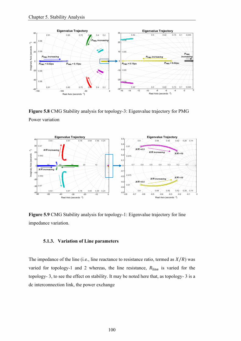
Chapter 5. Stability Analysis
100
-150 -100 -50 0-60
-40
-20
0
20
40
600.2
0.2
0.4
0.4
0.58
0.580.72
0.72
0.83
0.830.91
0.91
0.96
0.99
0.96
0.99
lma
gin
ary
Axis
(se
con
ds
)-1
Eigenvalue Trajectory
PPMG = 0.02pu
PPMG increasing
PPMG increasing
PPMG = 0.15pu
Real Axis (seconds -1)
-16 -14 -12 -10 -8 -6 -4 -2 0-30
-20
-10
0
10
20
300.045
0.0450.1
0.1
0.15
0.15
0.22
0.22
0.3
0.30.42
0.42
0.58
0.85
0.85
0.58
Eigenvalue Trajectory
PPMG
increasing
PPMG = 0.02puPPMG = 0.15pu
PPMG increasing
Real Axis (seconds -1)
Figure 5.8 CMG Stability analysis for topology-3: Eigenvalue trajectory for PMG
Power variation
-0.8 -0.7 -0.6 -0.5 -0.4 -0.3 -0.2 -0.1 0-0.5
-0.4
-0.3
-0.2
-0.1
0
0.1
0.2
0.3
0.4
0.5
0.14
0.14
0.1
0.28
0.28
0.2
0.42
0.42
0.3
0.56
0.56
0.4
0.68
0.68
0.50.6
0.8
0.8
0.7
0.975
0.975
0.91
0.91
Eigenvalue Trajectory
lma
gin
ary
Axis
(se
con
ds
)-1
-40 -30 -20 -10 0-50-60
-30
-20
-10
0
10
20
30
40
-40
Real Axis (seconds -1)
Eigenvalue Trajectory
Real Axis (seconds -1)
X/R increasing
X/R increasing
X/R increasing
X/R increasing
X/R =0.5
X/R =10
X/R =0.5
X/R =10
Figure 5.9 CMG Stability analysis for topology-1: Eigenvalue trajectory for line
impedance variation.
5.1.3. Variation of Line parameters
The impedance of the line (i.e., line reactance to resistance ratio, termed as 𝑋 𝑅⁄ ) was
varied for topology-1 and 2 whereas, the line resistance, 𝑅line is varied for the
topology- 3, to see the effect on stability. It may be noted here that, as topology- 3 is a
dc interconnection link, the power exchange
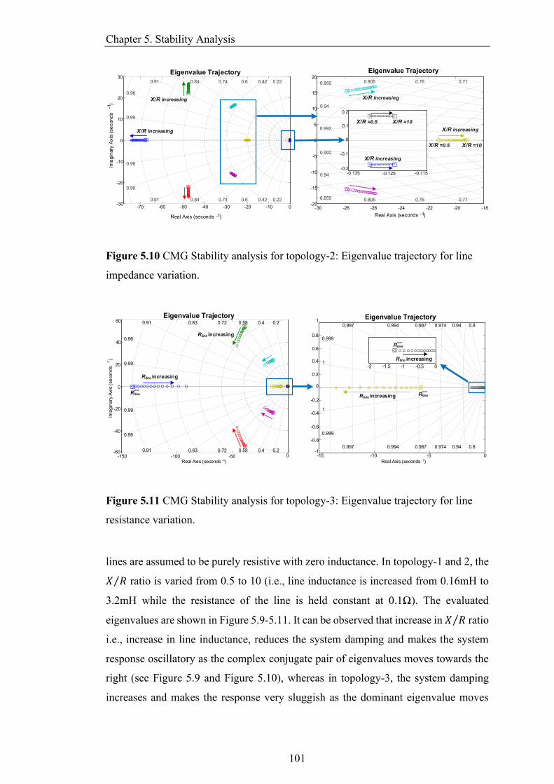
Chapter 5. Stability Analysis
101
-70 -60 -50 -40 -30 -20 -10 0-30
-20
-10
0
10
20
300.22
0.220.42
0.420.6
0.60.74
0.74
0.84
0.840.91
0.91
0.99
0.96
0.96
0.99
-30 -28 -26 -24 -22 -20 -18-20
-15
-10
-5
0
5
10
15
20
0.71
0.71
0.76
0.760.805
0.8050.855
0.992
0.992
0.855
0.94
0.94
Eigenvalue TrajectoryEigenvalue Trajectory
-0.135 -0.125 -0.115-0.2
-0.1
0
0.1
0.2lm
agin
ary
Axis
(se
con
ds
)-1
Real Axis (seconds -1) Real Axis (seconds -1)
X/R increasing
X/R increasing
X/R increasing
X/R increasing
X/R =0.5 X/R =10
X/R =0.5 X/R =10
X/R increasing
Figure 5.10 CMG Stability analysis for topology-2: Eigenvalue trajectory for line
impedance variation.
-150 -100 -50 0-60
-40
-20
0
20
40
60
0.2
0.20.4
0.4
0.58
0.58
0.72
0.72
0.83
0.830.91
0.91
0.99
0.96
0.96
0.99
-15 -10 -5 0-1
-0.8
-0.6
-0.4
-0.2
0
0.2
0.4
0.6
0.8
1
0.8
0.80.94
0.94
0.974
0.9740.987
0.9870.994
0.994
0.997
0.997
0.999
0.999
1
1
Rline increasing
lmagin
ary
Axis
(seconds
)-1
Real Axis (seconds -1)
-2 -1.5 -1 -0.5 0
Rline increasing
Rline increasing
Rline increasing
no m
Rline no m
Rline
no m
Rline
Eigenvalue Trajectory Eigenvalue Trajectory
Real Axis (seconds -1)
Figure 5.11 CMG Stability analysis for topology-3: Eigenvalue trajectory for line
resistance variation.
lines are assumed to be purely resistive with zero inductance. In topology-1 and 2, the
𝑋 𝑅⁄ ratio is varied from 0.5 to 10 (i.e., line inductance is increased from 0.16mH to
3.2mH while the resistance of the line is held constant at 0.1Ω). The evaluated
eigenvalues are shown in Figure 5.9-5.11. It can be observed that increase in 𝑋 𝑅⁄ ratio
i.e., increase in line inductance, reduces the system damping and makes the system
response oscillatory as the complex conjugate pair of eigenvalues moves towards the
right (see Figure 5.9 and Figure 5.10), whereas in topology-3, the system damping
increases and makes the response very sluggish as the dominant eigenvalue moves
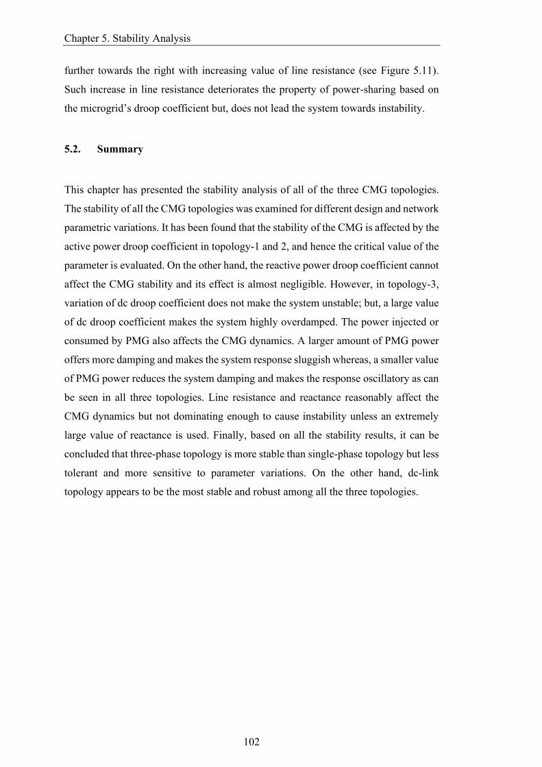
Chapter 5. Stability Analysis
102
further towards the right with increasing value of line resistance (see Figure 5.11).
Such increase in line resistance deteriorates the property of power-sharing based on
the microgrid’s droop coefficient but, does not lead the system towards instability.
5.2. Summary
This chapter has presented the stability analysis of all of the three CMG topologies.
The stability of all the CMG topologies was examined for different design and network
parametric variations. It has been found that the stability of the CMG is affected by the
active power droop coefficient in topology-1 and 2, and hence the critical value of the
parameter is evaluated. On the other hand, the reactive power droop coefficient cannot
affect the CMG stability and its effect is almost negligible. However, in topology-3,
variation of dc droop coefficient does not make the system unstable; but, a large value
of dc droop coefficient makes the system highly overdamped. The power injected or
consumed by PMG also affects the CMG dynamics. A larger amount of PMG power
offers more damping and makes the system response sluggish whereas, a smaller value
of PMG power reduces the system damping and makes the response oscillatory as can
be seen in all three topologies. Line resistance and reactance reasonably affect the
CMG dynamics but not dominating enough to cause instability unless an extremely
large value of reactance is used. Finally, based on all the stability results, it can be
concluded that three-phase topology is more stable than single-phase topology but less
tolerant and more sensitive to parameter variations. On the other hand, dc-link
topology appears to be the most stable and robust among all the three topologies.

Chapter 6. Sensitivity Analysis
103
Chapter 6 Sensitivity Analysis
This chapter presents the sensitivity analyses to demonstrate and validate the
performance of the three proposed topologies in terms of several key design and
operational factors. Sensitivity analysis reveals the system operation robustness
against the variation of some network and design parameters. The findings of this
chapter help us in selecting the suitable network parameters for a robust operation. In
this study, sensitivity analysis reveals several key design factors that govern and affect
the performance of the CMG.
6.1. Sensitivity Analysis
The sensitivity of the power exchange link and employed control strategy for all the
three topologies against the design and operational parameters has been analysed. The
objective is to determine how the variation of the interconnecting line impedance (i.e.,
the distance of the microgrids from each other) and the amount of power delivered or
absorbed by a PMG affect the power exchange link’s performance. The line loss, the
amount of power delivered/absorbed from HMGs to PMG, the LSC’s voltage and
droop angle, the HMG’s frequency, dc-link voltage, and finally error in power-sharing
based on their droop ratio are evaluated in the sensitivity analysis. The obtained results
are shown in Figure 6.1-6.14.
The study is carried out for all three CMG topologies for a scenario where two HMGs
are supporting one PMG while sharing the power with a droop ratio of 2:1. The results
show that the power-sharing among the HMGs based on their droop ratios is affected
to some extent as the impedance of the interconnecting lines (i.e., the distance among
the microgrids) is increased in the case of topology-1 and 2. The error in power-sharing
stays within the limit due to the employed modified angle droop control technique
using virtual inductance which minimizes the error margin. It can be noted here that,
Chapter 6. Sensitivity Analysis
104
conventional angle droop technique is highly sensitive to the magnitude of the line
impedances and for the technique to be accurate and applicable, the line reactance
should be several times larger than the resistance, which may not be always feasible
for practical CMG networks. Moreover, a larger value of droop coefficients drives the
system towards instability. To ensure adequate stability margins, droop coefficients
are selected to be small enough, but the sharing of the desired power among the
microgrids according to their droop coefficients will be lost. Hence, to ensure the
desired power-sharing among the HMGs, the modified angle droop method is
employed. One of the main objectives of the sensitivity analysis is to demonstrate the
ability to share power among the HMGs operating under the modified angle droop
while line impedances are varied, and the ratio of line resistance to reactance is larger
than unity.
However, in the case of topology- 3, such error in power-sharing is substantially larger
as the conventional dc voltage-power droop control technique is employed. The
conventional dc droop method is subjected to a mismatch in power-sharing and
experiences an uneven drop in dc-link voltage across the interconnecting link [114,
115]. Different values of resistances of the interconnecting lines (that is governed by
the distance among the microgrids forming the CMG) cause this voltage drop and such
voltage mismatch is responsible for the loss of the desired power-sharing according to
their droop coefficient among the microgrids. This mismatch in the droop voltage and
the resulting circulating current can be removed using the virtual resistance method
proposed in [115].
6.1.1. Line Parameter Variation
The first analysis is conducted for topology-1 and 2 together to make a comparison
between the sensitivity of the three-phase and single-phase ac interconnecting links for
variations of the same parameter. The HMG’s shared power through the link, LSC’s
droop angle and voltage, line loss, and error percentage in power-sharing as the
impedance varies are shown in Figure 6.1a-6.1h. For both topologies, the sensitivity
analysis was carried out considering a situation when one PMG is supported by two
HMGs. The nominal line impedance used in the simulation of case studies is used as
a reference and all parameters are normalised based on this value. The PMG power
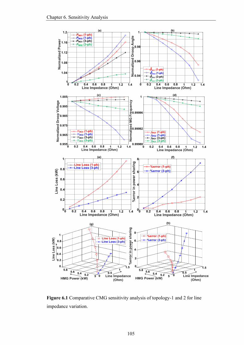
Chapter 6. Sensitivity Analysis
105
0 0.2 0.4 0.6 0.8 1 1.2 1.41
1.04
1.08
1.12
1.16
1.2(a)
PMG1 (1-ph)
PMG1 (3-ph)PMG2 (3-ph)
PMG2 (1-ph)
0.94
0.96
0.98
1(b)
δMG1 (1-ph)
δMG2 (1-ph)
δMG1 (3-ph)
δMG1 (3-ph)
No
rmalize
d P
ow
er
Line Impedance (Ohm)
No
rmalize
d D
roo
p A
ng
le
0 0.2 0.4 0.6 0.8 1 1.2 1.4Line Impedance (Ohm)
0.955
0.965
0.975
0.985
0.995
1.005(c)
VMG1 (1-ph)VMG2 (1-ph)VMG1 (3-ph)VMG1 (3-ph)
0.99988
0.99992
0.99996
1(d)
fMG1 (1-ph)fMG2 (1-ph)fMG1 (3-ph)fMG1 (3-ph)N
orm
alize
d D
roo
p V
olt
ag
e
No
rmalize
d M
G F
req
uen
cy
0 0.2 0.4 0.6 0.8 1 1.2 1.4Line Impedance (Ohm)
0 0.2 0.4 0.6 0.8 1 1.2 1.4Line Impedance (Ohm)
0
0.2
0.4
0.6
0.8
1(e)
Line Loss (1-ph)Line Loss (3-ph)
0
2
4
6
8(f)
Lin
e L
os
s (
kW
)
%e
rro
r in
po
wer
sh
ari
ng
0 0.2 0.4 0.6 0.8 1 1.2 1.4Line Impedance (Ohm)
0 0.2 0.4 0.6 0.8 1 1.2 1.4Line Impedance (Ohm)
%error (1-ph)
%error (3-ph)
Line Loss (1-ph)Line Loss (3-ph)
0
0.2
0.4
0.6
1
55.25.4
5.65.8
00.5
1.51
0.8
Line Impedance
(Ohm)HMG Power (kW)
Lin
e L
os
s (
kW
)
(g)
0
2
4
6
8
5.25.45.6
5.8
HMG Power (kW)5 0
0.5
1.51
Line Impedance
(Ohm)
%e
rro
r in
po
wer
sh
ari
ng
(h)
%error (1-ph)
%error (3-ph)
Figure 6.1 Comparative CMG sensitivity analysis of topology-1 and 2 for line
impedance variation.

Chapter 6. Sensitivity Analysis
106
Lin
e L
os
s (
kW
)
δM
G1 (
deg
)δ
MG
2 (
deg)
(a) (b)
1.85
0.3
0.2
0.1
1.81.75
1.7 3.353.40
3.45
0.3
0.25
0.2
0.15
0.1
0.05
56.06
56.02
55.98
55.94
1.851.8
1.751.7 3.35
3.403.45
56.06
56.04
56.02
55.96
56.00
55.98
55.94
56.2
56.0
55.8
1.851.8
1.751.7 3.35
3.403.45
56.25
56.15
56.05
55.95
55.85
PMG1(kW)
10
5
0
-5
10
6
2
-2
1.85 1.81.75 1.7 3.35
3.403.45%
err
or
in p
ow
er
sh
ari
ng
PMG2(kW)
VM
G1 (V
)V
MG
2 (V
)
340.1
339.9
339.7
340.1
339.9
339.7
340
339.8
339.61.85 1.81.75
1.7 3.353.40
3.45
341.5
340.5
339.5
1.85 1.81.75
1.7 3.35
3.40
3.45
341.5
340.5
339.5
341
340
339
(d)
PMG1(kW)PMG2(kW)
(e)
PMG1(kW) PMG2(kW) PMG1(kW) PMG2(kW)
(c)
PMG1(kW) PMG2(kW)PMG1(kW)
PMG2(kW)
(f)
Figure 6.2 Effect of line impedance variation on CMG network for topology-1
3.93.8
3.73.6
3.53.4
1.75
1.85
1.95
333.2
332.8
333
333.4
332.6
330
334
336
326
328
332
3.93.8
3.73.6
3.53.4
1.75
1.85
1.95
46
45
44
47
3.93.8
3.73.6
3.53.4
1.75
1.85
1.95
47.5
47
46.5
48
3.93.8
3.73.6
3.53.4
1.75
1.85
1.950
0.2
0.4
0.6
0.8
3.93.83.73.63.53.41.75
1.85
1.95
-2
0
2
4
-6
-4
-8
Lin
e L
os
s (
kW
)
PMG2(kW)PMG1(kW) PMG2(kW)PMG1(kW)
δM
G1 (
deg)
δM
G2 (
deg)
VM
G1
(V
)V
MG
2 (V
)
%e
rro
r in
po
wer
sh
ari
ng
3.93.8
3.73.6
3.53.41.75
1.851.95
PMG2(kW)PMG1(kW)
PMG2(kW)PMG1(kW) PMG2(kW)PMG1(kW)
PMG2(kW)PMG1(kW)
(a) (b) (c)
(d) (e) (f)
Figure 6.3 Effect of line impedance variation on CMG network for topology-2
demand is assumed to be 5kW. Referring to Figure. 6.1a - 6.1h, it can be seen that the
power delivered, and line loss increase as the line impedance is increased. To
accommodate the excess power required due to the increase in line loss, the
interconnecting line’s droop voltage and angle start to drop, according to their droop
coefficients. Hence, the frequency of each microgrid also starts to drop as the power
delivered by them increases due to increasing line loss. The variations in all parameters
are within the acceptable limit though the variations are more prominent in topology-
2 as compared to topology-1. Figure. 6.1e to 6.1f show the line loss and the percentage

Chapter 6. Sensitivity Analysis
107
of error in power-sharing according to their droop ratio, as the line impedance
increases. It can be observed from Figure. 6.1e to 6.1h that the line loss in the single-
phase link of topology-2 is higher as compared to the three-phase link of topology-1,
whereas the error in power-sharing is larger in the three-phase link. The line loss in a
three-phase link is less as the current is three times smaller than that of a single-phase
link. On the other hand, a single-phase link exhibits better accuracy in power-sharing
according to their droop coefficient among the microgrids. The Line loss and error
percentage are also shown as a 3D plot with respect to HMG’s total power due to line
impedance variation in Figure. 6.1g and 6.1h, respectively.
Figure 6.2 and Figure 6.3 show the surface plot of line loss, droop angle, voltage and
error percentage in power-sharing as the power delivered by two HMGs is varied due
to an increase in the line impedance in topology-1 and topology-2, respectively. It can
be observed that the droop angle plots of both HMG follow a similar pattern, whereas
the droop voltage plots are not similar. As the impedance of the interconnecting lines
is increased, the sharing of desired power, according to their droop coefficients, starts
to deviate slightly and produces an error. The reason behind such behaviour is that, as
the impedances of the lines become larger, the assumption of droop coefficients being
greater than the line reactance does not remain valid any longer, and thus, the property
of power-sharing, as the reciprocal of the droop coefficients, is lost. As can be seen
from Figure 6.2d, the variation of impedance causes an error of –5 to +10% in
topology-1 whereas, the error ranges from –8 to +4% in topology-2, as can be seen
from Figure 6.3d. In both topologies, the error stays in an acceptable range because of
the implemented modified angle droop, which is an effective way to ensure accurate
power-sharing among the microgrids.
The sensitivity analysis for topology-3 due to line resistance variation is shown in
Figure 6.4. It can be observed from Figure 6.4a to 6.4d that the line loss and power
delivered by each microgrid are increased as the line resistance (i.e., the distance of
the microgrids from each other) increases, whereas to accommodate the excess power
required due to line loss, the frequency and dc-link voltages start to drop according to
their droop coefficients values. The nominal PMG power demand is assumed to be
10kW. As the resistance of the interconnecting lines is increased, the property of
power-sharing based on their droop coefficients starts to become erroneous. This is
due to the fact that as the resistances of the lines become larger than droop coefficients
values, the property of power-sharing as the reciprocal of the droop coefficients, is not
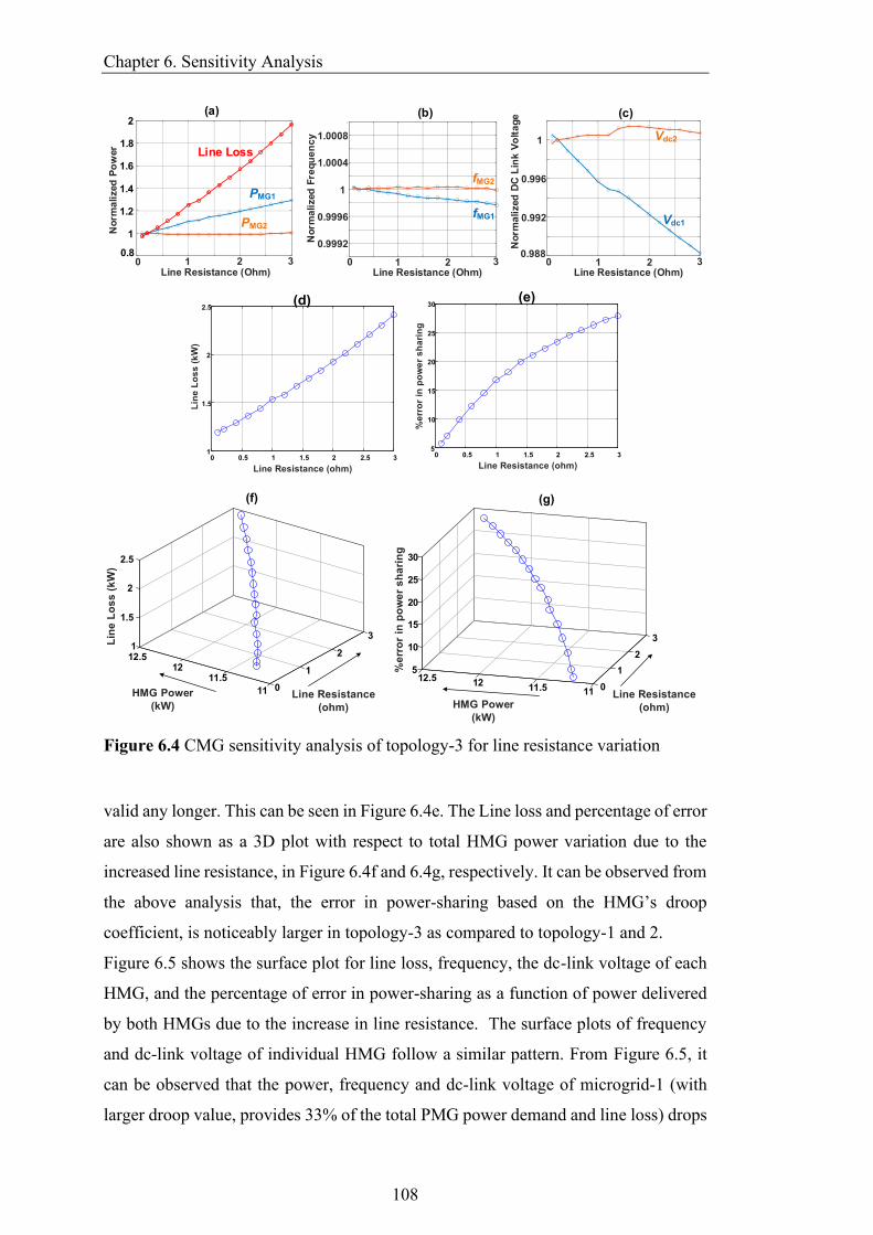
Chapter 6. Sensitivity Analysis
108
0.9992
0.9996
1
1.0004
1.0008
0.8
1
1.2
1.4
1.6
1.8
2
0.988
0.992
0.996
1
No
rma
lized
Po
wer
(a)
No
rma
lized
Fre
qu
en
cy
(b) (c)
No
rma
lized
DC
Lin
k V
olt
ag
e
Line Loss
PMG1
PMG2
fMG1
fMG2
Vdc2
Vdc1
0 1 2 3Line Resistance (Ohm)
0 1 2 3Line Resistance (Ohm)
0 1 2 3Line Resistance (Ohm)
0 0.5 1 1.5 2 2.5 31
1.5
2
2.5
0 0.5 1 1.5 2 2.5 35
10
15
20
25
30
Lin
e L
os
s (
kW
)
Line Resistance (ohm)
%e
rro
r in
po
we
r s
ha
rin
g
Line Resistance (ohm)
(d) (e)
3
2
15
10
12.5
15
12
20
11.5 0
25
11
30
31
12.5 2
1.5
12 111.5
2
011
2.5
Lin
e L
os
s (
kW
)
HMG Power
(kW)Line Resistance
(ohm)HMG Power
(kW)
%e
rro
r in
po
we
r s
ha
rin
g
Line Resistance
(ohm)
(f) (g)
Figure 6.4 CMG sensitivity analysis of topology-3 for line resistance variation
valid any longer. This can be seen in Figure 6.4e. The Line loss and percentage of error
are also shown as a 3D plot with respect to total HMG power variation due to the
increased line resistance, in Figure 6.4f and 6.4g, respectively. It can be observed from
the above analysis that, the error in power-sharing based on the HMG’s droop
coefficient, is noticeably larger in topology-3 as compared to topology-1 and 2.
Figure 6.5 shows the surface plot for line loss, frequency, the dc-link voltage of each
HMG, and the percentage of error in power-sharing as a function of power delivered
by both HMGs due to the increase in line resistance. The surface plots of frequency
and dc-link voltage of individual HMG follow a similar pattern. From Figure 6.5, it
can be observed that the power, frequency and dc-link voltage of microgrid-1 (with
larger droop value, provides 33% of the total PMG power demand and line loss) drops
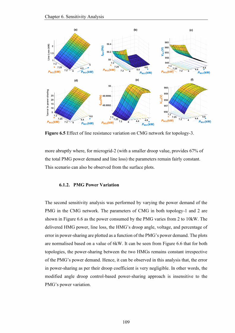
Chapter 6. Sensitivity Analysis
109
PMG1(kW)
%e
rro
r in
po
we
r s
ha
rin
g
50
49.9996
49.9992
50
4 4.4 4.8
7.37.25
7.2
50.5
50.4
50
50.1
50.2
50.3
50.4
50
50.2
PMG2(kW)
7.3
7.25
7.2 44.4
4.8
PMG1(kW)
7.3
7.25
7.2 44.5
5
PMG2(kW) PMG1(kW)
2
1.5
1
2.4
2.2
2.0
1.8
1.6
1.4
1.2
Lin
e L
os
s (
kW
)
960
959
957
958
960
959
958
957
956
44.4
4.87.3
7.257.2
PMG1(kW)
25
20
15
10
5
25
20
15
10
4
4.4
4.87.3
7.25
7.2PMG2(kW)PMG1(kW)
(a) (b)
f MG
2(H
z)
(d) (e)
Vd
c1(V
)
968
964
960
956
952
948
965
960
955
950
945
44.4
4.87.3
7.257.2PMG2(kW) PMG1(kW)
f MG
1(H
z)
(c)
PMG2(kW)
Vd
c2(V
)
PMG2(kW)
(f)
Figure 6.5 Effect of line resistance variation on CMG network for topology-3.
more abruptly where, for microgrid-2 (with a smaller droop value, provides 67% of
the total PMG power demand and line loss) the parameters remain fairly constant.
This scenario can also be observed from the surface plots.
6.1.2. PMG Power Variation
The second sensitivity analysis was performed by varying the power demand of the
PMG in the CMG network. The parameters of CMG in both topology-1 and 2 are
shown in Figure 6.6 as the power consumed by the PMG varies from 2 to 10kW. The
delivered HMG power, line loss, the HMG’s droop angle, voltage, and percentage of
error in power-sharing are plotted as a function of the PMG’s power demand. The plots
are normalised based on a value of 6kW. It can be seen from Figure 6.6 that for both
topologies, the power-sharing between the two HMGs remains constant irrespective
of the PMG’s power demand. Hence, it can be observed in this analysis that, the error
in power-sharing as per their droop coefficient is very negligible. In other words, the
modified angle droop control-based power-sharing approach is insensitive to the
PMG’s power variation.
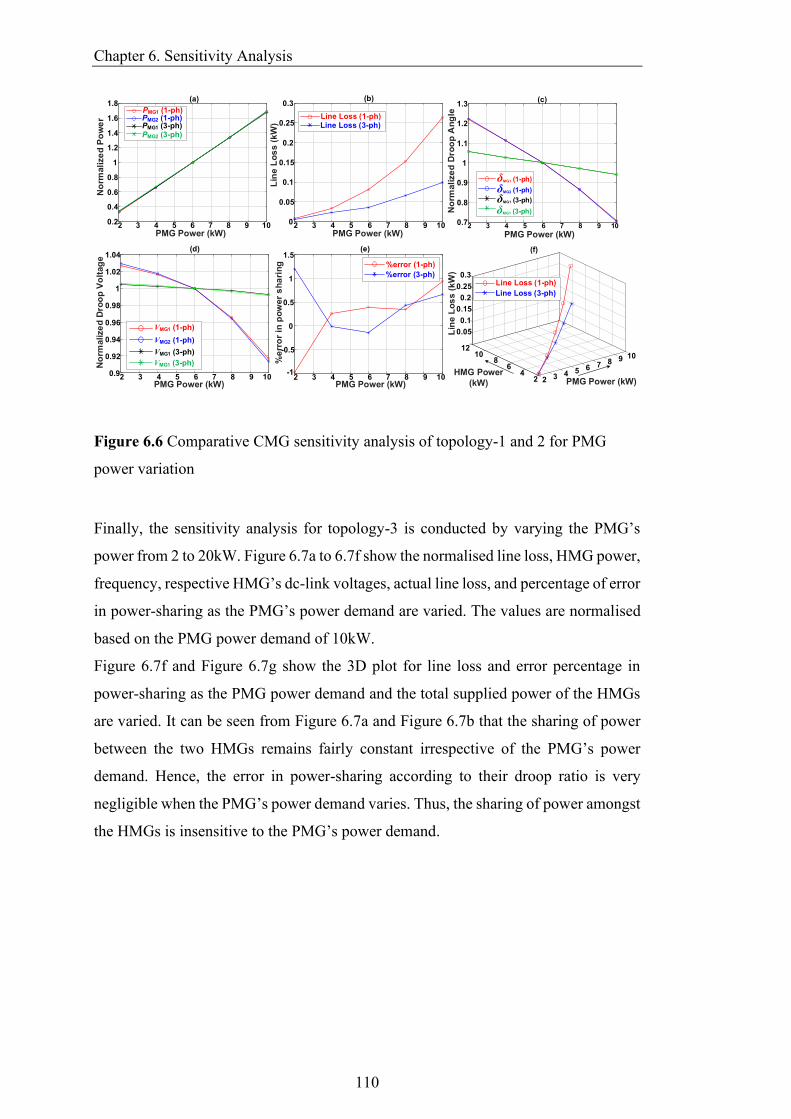
Chapter 6. Sensitivity Analysis
110
2 3 4 5 6 7 8 9 100.2
0.4
0.6
0.8
1
1.2
1.4
1.6
1.8(a)
2 3 4 5 6 7 8 9 100
0.05
0.1
0.15
0.2
0.25
0.3
2 3 4 5 6 7 8 9 100.9
0.92
0.94
0.96
0.98
1
1.02
1.04
2 3 4 5 6 7 8 9 100.7
0.8
0.9
1
1.1
1.2
1.3
2 3 4 5 6 7 8 9 10-1
-0.5
0
0.5
1
1.5
109876543224
68
10
0.25
0.2
0.15
0.1
0.3
0.05
12
PMG1 (1-ph)
PMG1 (3-ph)PMG2 (3-ph)
PMG2 (1-ph)
No
rmalize
d P
ow
er Line Loss (1-ph)
Line Loss (3-ph)
(b)
Lin
e L
os
s (
kW
)
No
rmalize
d D
roo
p V
olt
ag
e
VMG1 (1-ph)
VMG2 (1-ph)
VMG1 (3-ph)
VMG1 (3-ph)
No
rmalize
d D
roo
p A
ng
le
δMG1 (1-ph)
δMG2 (1-ph)
δMG1 (3-ph)
δMG1 (3-ph)
PMG Power (kW) PMG Power (kW)
(d) (e) (f)
%e
rro
r in
po
wer
sh
ari
ng %error (1-ph)
%error (3-ph)
PMG Power (kW)
PMG Power (kW)
PMG Power (kW)
Lin
e L
os
s (
kW
)
HMG Power
(kW) PMG Power (kW)
Line Loss (1-ph)
Line Loss (3-ph)
(c)
Figure 6.6 Comparative CMG sensitivity analysis of topology-1 and 2 for PMG
power variation
Finally, the sensitivity analysis for topology-3 is conducted by varying the PMG’s
power from 2 to 20kW. Figure 6.7a to 6.7f show the normalised line loss, HMG power,
frequency, respective HMG’s dc-link voltages, actual line loss, and percentage of error
in power-sharing as the PMG’s power demand are varied. The values are normalised
based on the PMG power demand of 10kW.
Figure 6.7f and Figure 6.7g show the 3D plot for line loss and error percentage in
power-sharing as the PMG power demand and the total supplied power of the HMGs
are varied. It can be seen from Figure 6.7a and Figure 6.7b that the sharing of power
between the two HMGs remains fairly constant irrespective of the PMG’s power
demand. Hence, the error in power-sharing according to their droop ratio is very
negligible when the PMG’s power demand varies. Thus, the sharing of power amongst
the HMGs is insensitive to the PMG’s power demand.
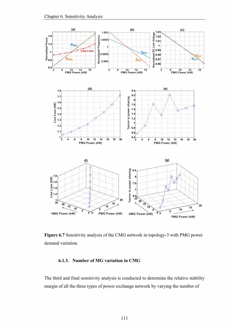
Chapter 6. Sensitivity Analysis
111
0.2
0.6
1
1.4
1.8
0.999
0.9995
1
1.0005
1.001
0.96
0.97
0.98
0.99
1
1.01
1.02
1.03(a) (b) (c)
No
rma
lized
Po
wer
No
rma
lized
Fre
qu
en
cy
No
rma
lized
DC
Lin
k V
olt
ag
e
Line Loss
2PMG Power (kW)
6 10 14 182PMG Power (kW)
6 10 14 18
PMG1
PMG2
fMG1
fMG2
Vdc2
Vdc1
2PMG Power (kW)
6 10 14 18
2 4 6 8 10 12 14 16 18 201
1.1
1.2
1.3
1.4
1.5
1.6
1.7
1.8
2 4 6 8 10 12 14 16 18 206.4
6.6
6.8
7
7.2
7.4
7.6
7.8
8
8.2
8.4
Lin
e L
os
s (
kW
)
%e
rro
r in
po
we
r s
ha
rin
g
(d) (e)
PMG Power (kW)PMG Power (kW)
6.525
7
20
7.5
15
8
2010
8.5
15105
50 0
20125 15
1.2
2015 10
1.4
10
1.6
55
1.8
00
Lin
e L
os
s (
kW
)
HMG Power (kW)
%e
rro
r in
po
we
r s
ha
rin
g
PMG Power (kW) HMG Power (kW)PMG Power (kW)
(f) (g)
Figure 6.7 Sensitivity analysis of the CMG network in topology-3 with PMG power
demand variation.
6.1.3. Number of MG variation in CMG
The third and final sensitivity analysis is conducted to determine the relative stability
margin of all the three types of power exchange network by varying the number of

Chapter 6. Sensitivity Analysis
112
-80
-60
-40
-20
0
20
-360
-270
-180
-90
0
100 101 102 103 104 105
Frequency (rad/s)
Ph
as
e(d
eg
)M
ag
nit
ud
e(d
b)
Stability Margins with Varying Number of MGs
(Power Loop- Topology-1)
GM-1GM-2
GM-3
PM-2
PM-1
PM-3
2-MG3-MG4-MG
2-MG3-MG4-MG
Figure 6.8 Stability margin comparison of the power control loop for topology-1
with varying number of microgrids to form CMG.
-40
-30
-20
-10
0
-450
-360
-270
-180
-90
0
Stability Margins with Varying Number of MGs
(Power Loop – Topology-2)
102 103 104 105
Frequency (rad/s)
Ph
as
e(d
eg
)M
ag
nit
ud
e(d
b)
PM-3PM-2
PM-1
GM-2GM-3
GM-1
2-MG3-MG4-MG
2-MG3-MG4-MG
Figure 6.9 Stability margin comparison of the power control loop for topology-2
with varying number of MGs to form CMG.

Chapter 6. Sensitivity Analysis
113
-150
-100
-50
0
50
100
101 102 103 104 105-720
-540
-360
-180
0
Frequency (rad/s)
Ph
as
e(d
eg
)M
ag
nit
ud
e(d
b)
GM-1GM-2GM-3
PM-3
PM-2 PM-1
2-MG3-MG4-MG
Stability Margins with Varying Number of MGs
(Power Loop- Topology-3)
2-MG3-MG4-MG
Figure 6.10 Stability margin comparison of the power control loop for topology-3
with varying number of MGs to form CMG.
interconnected microgrids to form the CMG. The two outer most control loops (i.e.
power and frequency) of LSCs (all the three topologies) and the dc power exchange
link (topology- 3) are examined in this analysis. The frequency responses of the power
control loop (Figure 3.6) with varying numbers of microgrids in all the topologies are
shown in Figure 6.8 – 6.10 whereas, responses of the frequency control loop (Figure
3.13) are shown in Figure 6.11-6.13, respectively. It can be observed from this analysis
that, the number of microgrids participating to form the CMG power exchange
network affects the dynamic response of the overall system and thus its gain and phase
margin. Even though the effect on gain and phase margin is not too significant but
coupling a large number of microgrids to form the CMG may result in a poor dynamic
response or in some cases may even make the network unstable. As can be seen from
Figure 6.8, the closed-loop phase margin of the power control loop reduces as the
number of microgrids in the CMG network is increased in the case of topology- 1. In
topology- 2, the phase margin increases for 3 microgrids whereas, it deteriorates when
4 microgrids are connected as can be seen from Figure 6.9. This implies that this
topology can offer the optimum phase margin and performance for 3 microgrids.
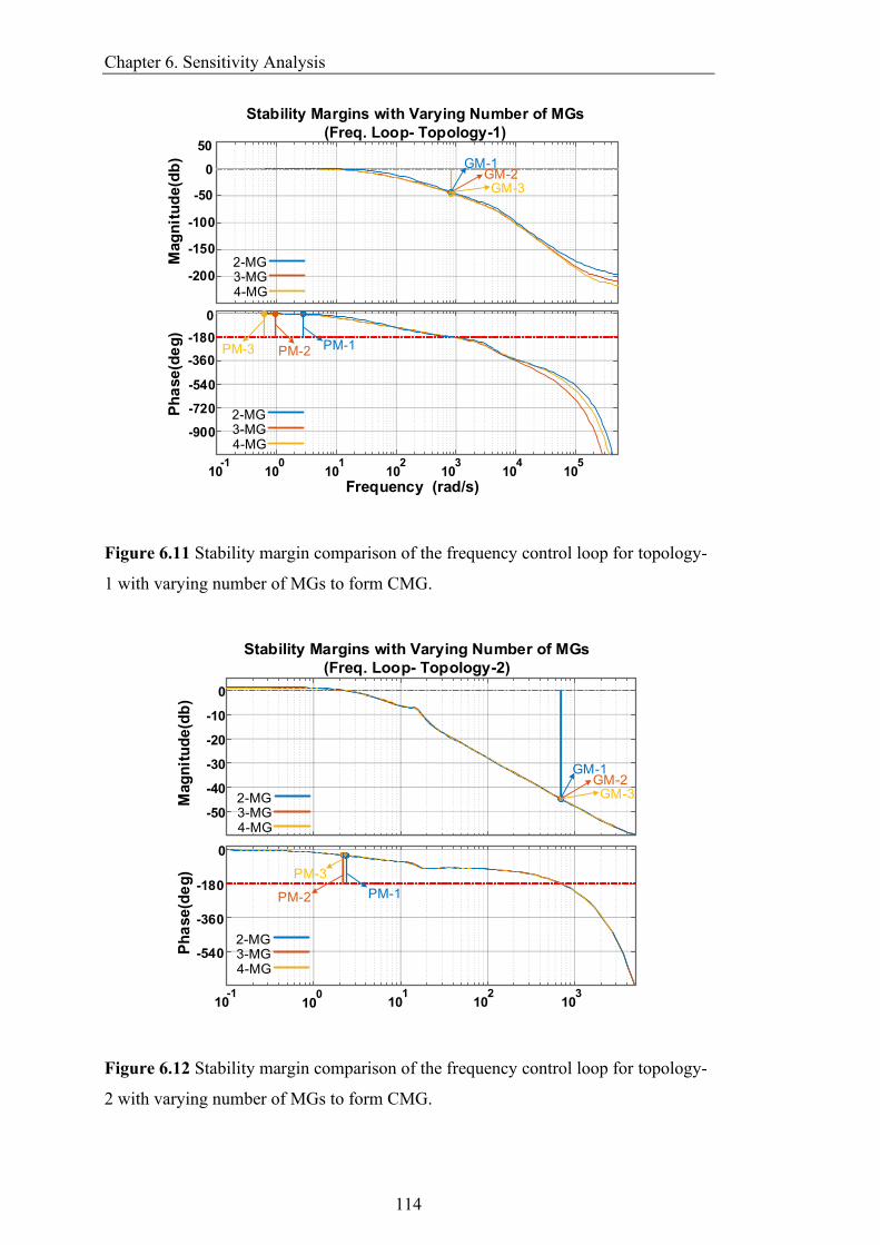
Chapter 6. Sensitivity Analysis
114
-200
-150
-100
-50
0
50
-900
-720
-540
-360
-180
0
10-1
100
104
102
103
101
105
Frequency (rad/s)
Stability Margins with Varying Number of MGs
(Freq. Loop- Topology-1)
Mag
nit
ud
e(d
b)
Ph
ase
(de
g)
GM-1GM-2GM-3
PM-3 PM-1PM-2
2-MG3-MG4-MG
2-MG3-MG4-MG
Figure 6.11 Stability margin comparison of the frequency control loop for topology-
1 with varying number of MGs to form CMG.
-50
-40
-30
-20
-10
0
-540
-360
-180
0
Stability Margins with Varying Number of MGs
(Freq. Loop- Topology-2)
10-1
100
102
103
101
PM-3
PM-1PM-2
GM-1GM-2GM-3
Mag
nit
ud
e(d
b)
Ph
ase
(de
g)
2-MG3-MG4-MG
2-MG3-MG4-MG
Figure 6.12 Stability margin comparison of the frequency control loop for topology-
2 with varying number of MGs to form CMG.

Chapter 6. Sensitivity Analysis
115
-50
0
50
-360
-180
Stability Margins with Varying Number of MGs
(Freq. Loop- Topology-3)
Frequency (rad/s)
0
Mag
nit
ud
e(d
b)
Ph
ase
(de
g)
2-MG3-MG4-MG
2-MG3-MG4-MG
PM-3
PM-1PM-2
GM-1GM-2GM-3
100
101
102
103
104
Figure 6.13 Stability margin comparison of the frequency control loop for topology-
3 with varying number of MGs to form CMG.
However, the phase margin increases with the increasing number of microgrids in the
case of topology- 3 as shown in Figure 6.10, but at the same time, it makes the system
response slower. For the frequency loop, the phase margin does not reduce but the
crossover frequency shifts towards the left for all the three topologies resulting in a
slower dynamic response as can be seen from Figure 6.11-6.13. Topology- 2 is the
least sensitive one as the crossover frequency remains almost fixed whereas, topology-
1 is the most sensitive one in this case. Overall, this study reveals that, if a large number
of microgrids are coupled together to form the CMG, the controllers need to be retuned
and redesigned in order to achieve the necessary gain and phase margin of the system.
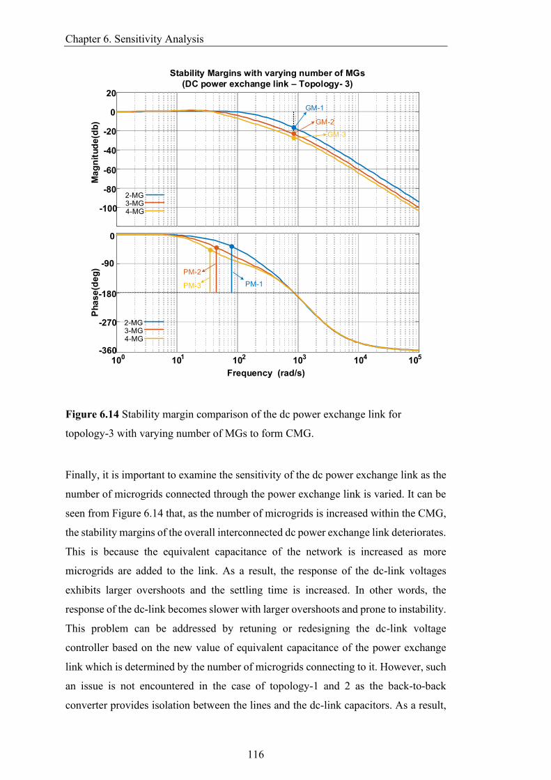
Chapter 6. Sensitivity Analysis
116
-100
-80
-60
-40
-20
0
20
100
101
102
103
104
105
-90
-180
-270
-360
Stability Margins with varying number of MGs
(DC power exchange link – Topology- 3)
Frequency (rad/s)
0
PM-3
PM-2
PM-1
GM-1
GM-2
GM-3
Ma
gn
itu
de
(db
)P
ha
se
(de
g)
2-MG3-MG4-MG
2-MG3-MG4-MG
Figure 6.14 Stability margin comparison of the dc power exchange link for
topology-3 with varying number of MGs to form CMG.
Finally, it is important to examine the sensitivity of the dc power exchange link as the
number of microgrids connected through the power exchange link is varied. It can be
seen from Figure 6.14 that, as the number of microgrids is increased within the CMG,
the stability margins of the overall interconnected dc power exchange link deteriorates.
This is because the equivalent capacitance of the network is increased as more
microgrids are added to the link. As a result, the response of the dc-link voltages
exhibits larger overshoots and the settling time is increased. In other words, the
response of the dc-link becomes slower with larger overshoots and prone to instability.
This problem can be addressed by retuning or redesigning the dc-link voltage
controller based on the new value of equivalent capacitance of the power exchange
link which is determined by the number of microgrids connecting to it. However, such
an issue is not encountered in the case of topology-1 and 2 as the back-to-back
converter provides isolation between the lines and the dc-link capacitors. As a result,
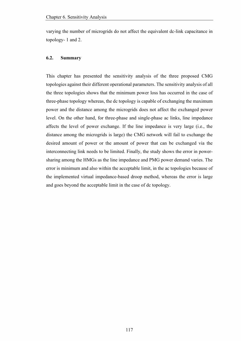
Chapter 6. Sensitivity Analysis
117
varying the number of microgrids do not affect the equivalent dc-link capacitance in
topology- 1 and 2.
6.2. Summary
This chapter has presented the sensitivity analysis of the three proposed CMG
topologies against their different operational parameters. The sensitivity analysis of all
the three topologies shows that the minimum power loss has occurred in the case of
three-phase topology whereas, the dc topology is capable of exchanging the maximum
power and the distance among the microgrids does not affect the exchanged power
level. On the other hand, for three-phase and single-phase ac links, line impedance
affects the level of power exchange. If the line impedance is very large (i.e., the
distance among the microgrids is large) the CMG network will fail to exchange the
desired amount of power or the amount of power that can be exchanged via the
interconnecting link needs to be limited. Finally, the study shows the error in power-
sharing among the HMGs as the line impedance and PMG power demand varies. The
error is minimum and also within the acceptable limit, in the ac topologies because of
the implemented virtual impedance-based droop method, whereas the error is large
and goes beyond the acceptable limit in the case of dc topology.
Chapter 7. Conclusions and recommendations
118
Chapter 7 Conclusions and recommendations
This chapter summarises the important findings of this thesis. Based on different
findings and observations, some recommendations are also made for future
researchers.
7.1. Conclusions
A standalone microgrid is an effective approach to electrify remote and isolated
communities. It can integrate various renewable-based distributed energy resources
along with required energy storages and coordinate them to supply its demand. The
uncertainties of load demand and the power generated by the renewable sources cause
the overloading and over-generation situations in standalone remote area microgrids
Such problems make it difficult to maintain the voltage and frequency within the
desirable range and if not alleviated, it may even lead the whole system towards
instability.
This thesis reports the newly developed control techniques for power electronic
converters used for interconnecting neighbouring autonomously operating microgrids
to prevent unacceptable voltage and frequency deviation due to overloading and over-
generations. The thesis has analysed and discussed three different approaches to
forming a system of interconnected microgrid networks that will facilitate power
exchange through a power electronic converter-based interface only when one or more
of those microgrids are experiencing either overloading due to lack of adequate power
generation or over-generation from its renewable-based sources. The studied
topologies provide the necessary isolation of the microgrids so that each microgrid can
operate autonomously according to its own internal standards and control techniques
while enabling power-sharing amongst them. The control mechanism of each structure
is based on a decentralised local frequency monitoring and regulation technique for
Chapter 7. Conclusions and recommendations
119
the individual microgrids that eliminates the requirement for a centralised control or
data communication infrastructure. Also, a suitable framework has been discussed that
ensures adequate and proper power-sharing among the microgrids based on droop
control mechanism when more than one microgrid will support overloaded or over-
generating microgrid(s). Thus, the approach reduces or prevents load-shedding or
curtailment of renewable sources when microgrid experiences such overloading or
excessive generation. The mechanism includes an approach to realise the desired
power-sharing ratio among multiple HMGs and various control techniques to detect
the microgrid’s status. At the same time, it also determines the required level of active
power that needs to be exchanged to support the PMG which will operate in the
constant PQ control mode. Such transitions between the various modes of operation of
the microgrids are achieved based on measuring the local parameters only. The
simulation-based case studies are carried out in PSIM® to validate the efficacy of the
discussed approaches in addressing the problems of the unacceptable frequency
deviation in the microgrids, following a power excess or shortfall. The studies
demonstrate the success of the proposed technique under various loading conditions.
The stability analysis has identified the system parameters that are responsible to affect
the dynamics of the CMG network. The stability studies show that the stability of the
CMG in topology- 1 and 2, is mostly affected by the active power droop coefficient,
while the reactive power droop coefficient does not affect the CMG stability
significantly. In topology- 3, a larger value of droop coefficient makes the system
highly overdamped but does not drive the system towards instability. The power
consumed and injected by a PMG also affects the system dynamics. A larger PMG
power provides more damping and makes the system’s response relatively slower,
whereas a smaller power exhibits smaller system damping and hence response
becomes oscillatory. Such phenomena can be seen for all three topologies. The line
impedance also affects the CMG dynamics for topology- 1 and 2, but the impact is not
too strong to cause instability. However, a larger value of the X/R ratio reduces the
system damping and hence makes the system response oscillatory. The variation of
line resistance in the case of topology- 3 makes the system overdamped and very
sluggish but does not drives the system towards instability.
Finally, the performed sensitivity analysis of the CMG topologies demonstrates an
acceptable variation of the different system parameters and quantities with respect to
the variation of design and operational factors. Based on the study results, it can be
Chapter 7. Conclusions and recommendations
120
concluded that the proposed technique offers a considerably robust performance
against variations of those parameters. Between topology-1 and 2, the variations are
more prominent in topology- 2, whereas smaller variations are observed in the case of
topology- 1. Both topology-1 and 2 equally performed in terms of power-sharing
whereas the line losses are 3-4 times higher in the case of topology- 2. On the other
hand, topology- 3 is robust in terms of PMG power variation but very sensitive for the
variation of line resistance. It was observed that, as the line resistance is increased in
topology- 3, the property of power-sharing based on desired droop coefficient starts to
exhibit errors. The final sensitivity study was performed to observe the effect of
varying the number of microgrids to form the CMG and it was found that the stability
margins remain within the acceptable limit for all three topologies.
7.2. Recommendations
Based on the findings of this research, the following topics can be recommended as
protentional future research avenues:
• This thesis has fully focused on the technical aspects of the proposal and was not
aiming at a techno-economic study. A future research can be on evaluating the
economic and cost-benefit analysis of all introduced three topologies to select
the most cost optimum topology for a given network.
• The methods in this thesis were based on a decentralised approach. Developing
a control mechanism for CMGs assuming the presence of a distributed or semi-
decentralised controller can be the topic of a future research.

Appendix
121
Appendix
The network and controller parameters used in the simulation studies are given in
Table A.1.
Table A.1 Technical data of network under consideration
Network 𝑉rated = 415V, 𝑓nom = 50Hz, 𝑓min = 49.5Hz, 𝑓max = 50.2Hz,
𝑃max = 100kW, 𝑉dc = 1.5kV, 𝑍MG = 0.1 + 𝑗0.5Ω,
𝑍line = 0.1 + 𝑗0.08Ω
DER droop 𝑚 = 0.01Hz/kW, 𝑛 = 0.1V/kVAR
Angle droop 𝑚d = 0.002 rad/kW, 𝑛d = 0.004V/kVAR
DC Droop Parameters 𝑚MG−1 = 2.5V/kW, 𝑚MG−2 = 5V/kW, 𝑚MG−3 = 5V/kW
VSC and filters 𝑅f = 0.1Ω, 𝐿f = 2mH, 𝑅g(MSC) = 0.04Ω, 𝐿𝑔(MSC) = 1.36mH,
𝑅g(LSC) = 0.12Ω, 𝐿𝑔(LSC) = 10mH, 𝐶f = 25μF, 𝐶dc = 4700μF
Linear quadratic regulator gains 𝑘1 = 58.63, 𝑘2 = 97.18, 𝑘3 = 1.2, 𝜔𝑐 = 6283.2 rad/s
PI - PQ controller (MSC) Proportional Gain, 𝐾c = 0.628, Time Constant,
𝑇c = 0.034 s, 𝑓BW = 73.5Hz
PI - PQ controller (LSC) Proportional Gain, 𝐾c = 0.628, Time Constant,
𝑇c = 0.0834 s, 𝑓BW = 10Hz
Frequency controller 𝐾OL = 15k, 𝑇OL = 0.025 s, 𝜔OL = 314 rad/s, 𝐾OG = 20k, 𝑇OG =
0.05 s, 𝜔OG = 37.7 krad/s. 𝐾PLL = 5, 𝑇PLL = 0.02 s
Dc-link voltage controller 𝐾dc = 222, 𝜔z = 2.2rad/s, 𝜔p = 1000rad/s, 𝜏dc = 392.2ms,
𝑃so = 100kW, 𝑉d = 380V
References
122
References
[1] R.H. Lasseter, “Microgrids,” IEEE Power Engineering Society Winter Meeting.
Conference, vol. 1, pp. 305-308, 2002.
[2] R.H. Lasseter, and P. Piagi, “Microgrid: A conceptual solution,’ IEEE Power
Electronics Specialists Conference, vol. 6, pp. 4285-4291. 2004.
[3] Y. Yoldaş, A. Önen, S. M. Muyeen, A. V. Vasilakos, İ. Alan, “Enhancing smart
grid with microgrids: Challenges and opportunities”, Renew. Sustain. Energy
Rev., vol. 72, pp. 205-214, May 2017.
[4] L. Ali and F. Shahnia, “Determination of an economically-suitable and
sustainable standalone power system for an off-grid town in Western Australia,”
Renewable Energy, vol. 106, pp.243-254, 2017.
[5] L. Ali and F. Shahnia, “Selection of a suitable standalone power supply system
for an off-grid town in Western Australia,” 2016 IEEE 16th International
Conference on Environment and Electrical Engineering (EEEIC), 2016, pp. 1-6,
doi: 10.1109/EEEIC.2016.7555735.
[6] L. Ali and F. Shahnia, “Impact of annual load growth on selecting the suitable
sustainable standalone system for an off-grid town in Western Australia,” 2016
IEEE International Conference on Power System Technology (POWERCON),
2016, pp. 1-5, doi: 10.1109/POWERCON.2016.7754043.
[7] L. Ali, F. Shahnia, A. Arefi, H. Iu and T. Fernando, “Feasibility analysis of a
sustainable system for an Australian remote town,” 2017 3rd International
Conference on Power Generation Systems and Renewable Energy Technologies
(PGSRET), 2017, pp. 118-122, doi: 10.1109/PGSRET.2017.8251812.
[8] J.G. de Matos, F.S.F. de Silva, L.A. de S. Ribeiro, “Power control in ac isolated
microgrids with renewable energy sources and energy storage systems,” IEEE
Trans. Industrial Electronics, 62(6):3490-3498, 2015
[9] N. Eghtedarpour and E. Farjah, “Power Control and Management in a Hybrid
References
123
AC/DC Microgrid,” in IEEE Transactions on Smart Grid, vol. 5, no. 3, pp. 1494-
1505, May 2014, doi: 10.1109/TSG.2013.2294275.
[10] F. Katiraei and M. R. Iravani, “Power Management Strategies for a Microgrid
With Multiple Distributed Generation Units,” in IEEE Transactions on Power
Systems, vol. 21, no. 4, pp. 1821-1831, Nov. 2006, doi:
10.1109/TPWRS.2006.879260.
[11] R. P. S. Chandrasena, F. Shahnia, A. Ghosh and S. Rajakaruna, “Operation and
control of a hybrid AC-DC nanogrid for future community houses,” 2014
Australasian Universities Power Engineering Conference (AUPEC), 2014, pp.
1-6, doi: 10.1109/AUPEC.2014.6966617.
[12] R. P. S. Chandrasena, F. Shahnia, S. Rajakaruna and A. Ghosh, “Operation and
control of three phase microgrids consisting of single-phase DERs,” 2013 IEEE
8th International Conference on Industrial and Information Systems, 2013, pp.
599-604, doi: 10.1109/ICIInfS.2013.6732052.
[13] F. Shahnia, et al. “A three-phase community microgrid comprised of single-
phase energy resources with an uneven scattering amongst phases.” International
Journal of Electrical Power & Energy Systems 84 (2017): 267-283.
[14] M.F. Zia, E. Elbouchikhi and M. Benbouzid, “Microgrids energy management
systems: A critical review on methods, solutions, and prospects,” Applied
energy, vol. 22. 1033-1055, 2018.
[15] R. P. S. Chandrasena, F. Shahnia, S. Rajakaruna and A. Ghosh, “Control,
operation and power sharing among parallel converter-interfaced DERs in a
microgrid in the presence of unbalanced and harmonic loads,” 2013 Australasian
Universities Power Engineering Conference (AUPEC), 2013, pp. 1-6, doi:
10.1109/AUPEC.2013.6725382.
[16] S.A. Arefifar, Y.A.R.I. Mohamed, “DG mix, reactive sources and energy storage
units for optimizing microgrid reliability and supply security,” IEEE Trans.
Smart Grid, 5(4):1835-1844, 2014.
[17] F. Nejabatkhah and Y. W. Li, “Overview of Power Management Strategies of
Hybrid AC/DC Microgrid,” in IEEE Transactions on Power Electronics, vol. 30,
no. 12, pp. 7072-7089, Dec. 2015, doi: 10.1109/TPEL.2014.2384999.
[18] M. A. Shoeb, F. Shahnia and G. Shafiullah, “A Multilayer Preventive Control to
Regulate Voltage and Frequency in Autonomous Microgrids,” 2018
Australasian Universities Power Engineering Conference (AUPEC), 2018, pp.
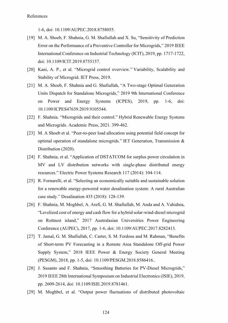
References
124
1-6, doi: 10.1109/AUPEC.2018.8758055.
[19] M. A. Shoeb, F. Shahnia, G. M. Shafiullah and X. Su, “Sensitivity of Prediction
Error on the Performance of a Preventive Controller for Microgrids,” 2019 IEEE
International Conference on Industrial Technology (ICIT), 2019, pp. 1717-1722,
doi: 10.1109/ICIT.2019.8755157.
[20] Kani, A. P., et al. “Microgrid control overview.” Variability, Scalability and
Stability of Microgrid. IET Press, 2019.
[21] M. A. Shoeb, F. Shahnia and G. Shafiullah, “A Two-stage Optimal Generation
Units Dispatch for Standalone Microgrids,” 2019 9th International Conference
on Power and Energy Systems (ICPES), 2019, pp. 1-6, doi:
10.1109/ICPES47639.2019.9105544.
[22] F. Shahnia. “Microgrids and their control.” Hybrid Renewable Energy Systems
and Microgrids. Academic Press, 2021. 399-462.
[23] M. A Shoeb et al. “Peer-to-peer load allocation using potential field concept for
optimal operation of standalone microgrids.” IET Generation, Transmission &
Distribution (2020).
[24] F. Shahnia, et al. “Application of DSTATCOM for surplus power circulation in
MV and LV distribution networks with single-phase distributed energy
resources.” Electric Power Systems Research 117 (2014): 104-114.
[25] R. Fornarelli, et al. “Selecting an economically suitable and sustainable solution
for a renewable energy-powered water desalination system: A rural Australian
case study.” Desalination 435 (2018): 128-139.
[26] F. Shahnia, M. Moghbel, A. Arefi, G. M. Shafiullah, M. Anda and A. Vahidnia,
“Levelized cost of energy and cash flow for a hybrid solar-wind-diesel microgrid
on Rottnest island,” 2017 Australasian Universities Power Engineering
Conference (AUPEC), 2017, pp. 1-6, doi: 10.1109/AUPEC.2017.8282413.
[27] T. Jamal, G. M. Shafiullah, C. Carter, S. M. Ferdous and M. Rahman, “Benefits
of Short-term PV Forecasting in a Remote Area Standalone Off-grid Power
Supply System,” 2018 IEEE Power & Energy Society General Meeting
(PESGM), 2018, pp. 1-5, doi: 10.1109/PESGM.2018.8586416..
[28] J. Susanto and F. Shahnia, “Smoothing Batteries for PV-Diesel Microgrids,”
2019 IEEE 28th International Symposium on Industrial Electronics (ISIE), 2019,
pp. 2609-2614, doi: 10.1109/ISIE.2019.8781461.
[29] M. Moghbel, et al. “Output power fluctuations of distributed photovoltaic
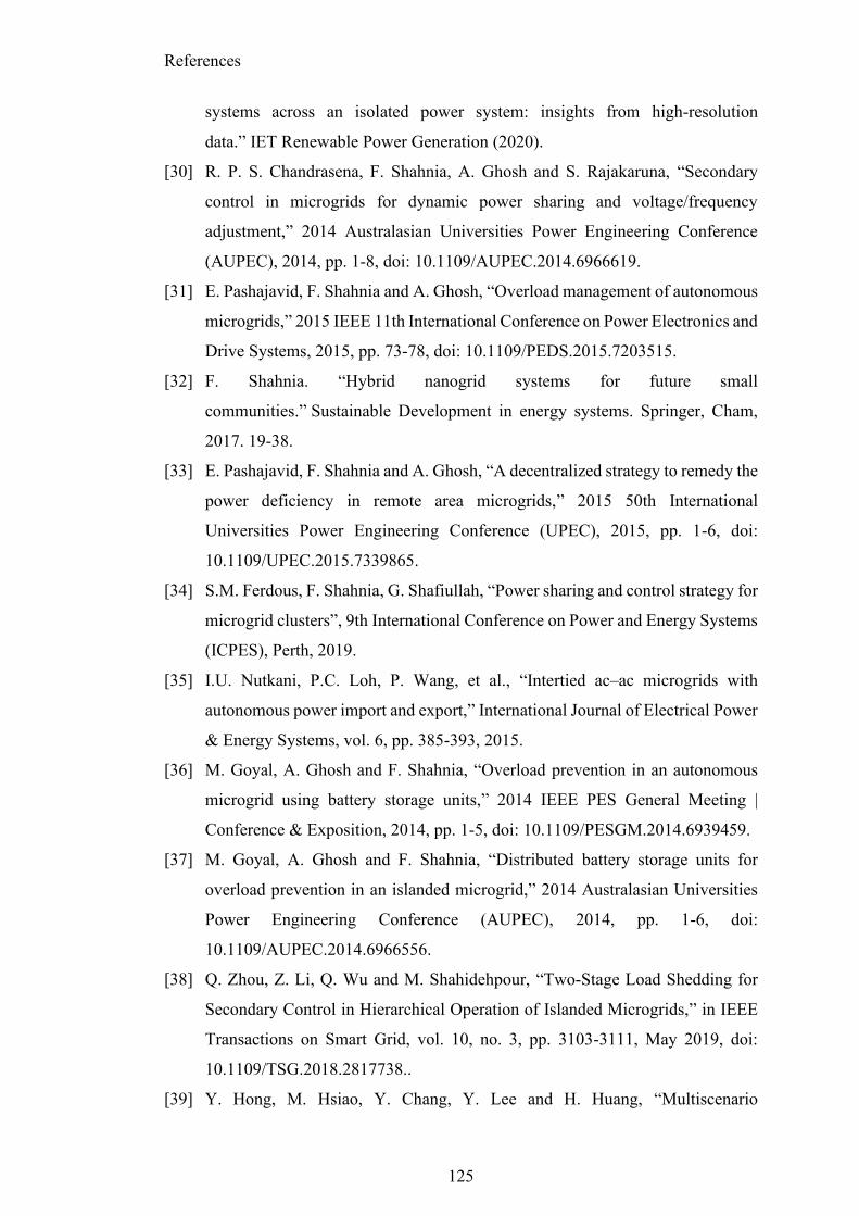
References
125
systems across an isolated power system: insights from high-resolution
data.” IET Renewable Power Generation (2020).
[30] R. P. S. Chandrasena, F. Shahnia, A. Ghosh and S. Rajakaruna, “Secondary
control in microgrids for dynamic power sharing and voltage/frequency
adjustment,” 2014 Australasian Universities Power Engineering Conference
(AUPEC), 2014, pp. 1-8, doi: 10.1109/AUPEC.2014.6966619.
[31] E. Pashajavid, F. Shahnia and A. Ghosh, “Overload management of autonomous
microgrids,” 2015 IEEE 11th International Conference on Power Electronics and
Drive Systems, 2015, pp. 73-78, doi: 10.1109/PEDS.2015.7203515.
[32] F. Shahnia. “Hybrid nanogrid systems for future small
communities.” Sustainable Development in energy systems. Springer, Cham,
2017. 19-38.
[33] E. Pashajavid, F. Shahnia and A. Ghosh, “A decentralized strategy to remedy the
power deficiency in remote area microgrids,” 2015 50th International
Universities Power Engineering Conference (UPEC), 2015, pp. 1-6, doi:
10.1109/UPEC.2015.7339865.
[34] S.M. Ferdous, F. Shahnia, G. Shafiullah, “Power sharing and control strategy for
microgrid clusters”, 9th International Conference on Power and Energy Systems
(ICPES), Perth, 2019.
[35] I.U. Nutkani, P.C. Loh, P. Wang, et al., “Intertied ac–ac microgrids with
autonomous power import and export,” International Journal of Electrical Power
& Energy Systems, vol. 6, pp. 385-393, 2015.
[36] M. Goyal, A. Ghosh and F. Shahnia, “Overload prevention in an autonomous
microgrid using battery storage units,” 2014 IEEE PES General Meeting |
Conference & Exposition, 2014, pp. 1-5, doi: 10.1109/PESGM.2014.6939459.
[37] M. Goyal, A. Ghosh and F. Shahnia, “Distributed battery storage units for
overload prevention in an islanded microgrid,” 2014 Australasian Universities
Power Engineering Conference (AUPEC), 2014, pp. 1-6, doi:
10.1109/AUPEC.2014.6966556.
[38] Q. Zhou, Z. Li, Q. Wu and M. Shahidehpour, “Two-Stage Load Shedding for
Secondary Control in Hierarchical Operation of Islanded Microgrids,” in IEEE
Transactions on Smart Grid, vol. 10, no. 3, pp. 3103-3111, May 2019, doi:
10.1109/TSG.2018.2817738..
[39] Y. Hong, M. Hsiao, Y. Chang, Y. Lee and H. Huang, “Multiscenario
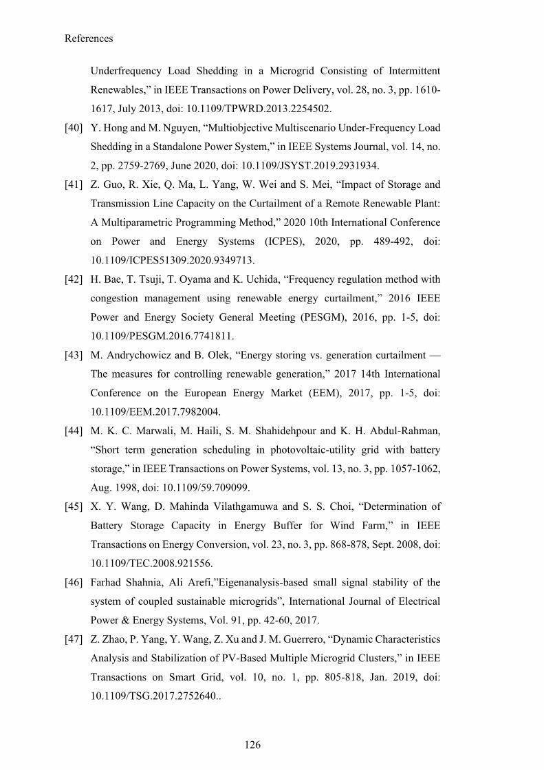
References
126
Underfrequency Load Shedding in a Microgrid Consisting of Intermittent
Renewables,” in IEEE Transactions on Power Delivery, vol. 28, no. 3, pp. 1610-
1617, July 2013, doi: 10.1109/TPWRD.2013.2254502.
[40] Y. Hong and M. Nguyen, “Multiobjective Multiscenario Under-Frequency Load
Shedding in a Standalone Power System,” in IEEE Systems Journal, vol. 14, no.
2, pp. 2759-2769, June 2020, doi: 10.1109/JSYST.2019.2931934.
[41] Z. Guo, R. Xie, Q. Ma, L. Yang, W. Wei and S. Mei, “Impact of Storage and
Transmission Line Capacity on the Curtailment of a Remote Renewable Plant:
A Multiparametric Programming Method,” 2020 10th International Conference
on Power and Energy Systems (ICPES), 2020, pp. 489-492, doi:
10.1109/ICPES51309.2020.9349713.
[42] H. Bae, T. Tsuji, T. Oyama and K. Uchida, “Frequency regulation method with
congestion management using renewable energy curtailment,” 2016 IEEE
Power and Energy Society General Meeting (PESGM), 2016, pp. 1-5, doi:
10.1109/PESGM.2016.7741811.
[43] M. Andrychowicz and B. Olek, “Energy storing vs. generation curtailment —
The measures for controlling renewable generation,” 2017 14th International
Conference on the European Energy Market (EEM), 2017, pp. 1-5, doi:
10.1109/EEM.2017.7982004.
[44] M. K. C. Marwali, M. Haili, S. M. Shahidehpour and K. H. Abdul-Rahman,
“Short term generation scheduling in photovoltaic-utility grid with battery
storage,” in IEEE Transactions on Power Systems, vol. 13, no. 3, pp. 1057-1062,
Aug. 1998, doi: 10.1109/59.709099.
[45] X. Y. Wang, D. Mahinda Vilathgamuwa and S. S. Choi, “Determination of
Battery Storage Capacity in Energy Buffer for Wind Farm,” in IEEE
Transactions on Energy Conversion, vol. 23, no. 3, pp. 868-878, Sept. 2008, doi:
10.1109/TEC.2008.921556.
[46] Farhad Shahnia, Ali Arefi,”Eigenanalysis-based small signal stability of the
system of coupled sustainable microgrids”, International Journal of Electrical
Power & Energy Systems, Vol. 91, pp. 42-60, 2017.
[47] Z. Zhao, P. Yang, Y. Wang, Z. Xu and J. M. Guerrero, “Dynamic Characteristics
Analysis and Stabilization of PV-Based Multiple Microgrid Clusters,” in IEEE
Transactions on Smart Grid, vol. 10, no. 1, pp. 805-818, Jan. 2019, doi:
10.1109/TSG.2017.2752640..
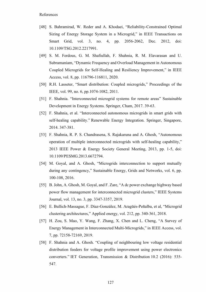
References
127
[48] S. Bahramirad, W. Reder and A. Khodaei, “Reliability-Constrained Optimal
Sizing of Energy Storage System in a Microgrid,” in IEEE Transactions on
Smart Grid, vol. 3, no. 4, pp. 2056-2062, Dec. 2012, doi:
10.1109/TSG.2012.2217991.
[49] S. M. Ferdous, G. M. Shafiullah, F. Shahnia, R. M. Elavarasan and U.
Subramaniam, “Dynamic Frequency and Overload Management in Autonomous
Coupled Microgrids for Self-Healing and Resiliency Improvement,” in IEEE
Access, vol. 8, pp. 116796-116811, 2020.
[50] R.H. Lasseter, “Smart distribution: Coupled microgrids,” Proceedings of the
IEEE, vol. 99, no. 6, pp.1074-1082, 2011.
[51] F. Shahnia. “Interconnected microgrid systems for remote areas” Sustainable
Development in Energy Systems. Springer, Cham, 2017. 39-63.
[52] F. Shahnia, et al. “Interconnected autonomous microgrids in smart grids with
self-healing capability.” Renewable Energy Integration. Springer, Singapore,
2014. 347-381.
[53] F. Shahnia, R. P. S. Chandrasena, S. Rajakaruna and A. Ghosh, “Autonomous
operation of multiple interconnected microgrids with self-healing capability,”
2013 IEEE Power & Energy Society General Meeting, 2013, pp. 1-5, doi:
10.1109/PESMG.2013.6672794.
[54] M. Goyal, and A. Ghosh, “Microgrids interconnection to support mutually
during any contingency,” Sustainable Energy, Grids and Networks, vol. 6, pp.
100-108, 2016.
[55] B. John, A. Ghosh, M. Goyal, and F. Zare, “A dc power exchange highway based
power flow management for interconnected microgrid clusters,” IEEE Systems
Journal, vol. 13, no. 3, pp. 3347-3357, 2019.
[56] E. Bullich-Massague, F. Díaz-González, M. Aragüés-Peñalba, et al, “Microgrid
clustering architectures,” Applied energy, vol. 212, pp. 340-361, 2018.
[57] H. Zou, S. Mao, Y. Wang, F. Zhang, X. Chen and L. Cheng, “A Survey of
Energy Management in Interconnected Multi-Microgrids,” in IEEE Access, vol.
7, pp. 72158-72169, 2019.
[58] F. Shahnia and A. Ghosh. “Coupling of neighbouring low voltage residential
distribution feeders for voltage profile improvement using power electronics
converters.” IET Generation, Transmission & Distribution 10.2 (2016): 535-
547.
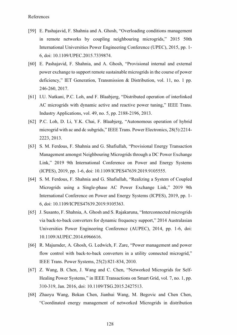
References
128
[59] E. Pashajavid, F. Shahnia and A. Ghosh, “Overloading conditions management
in remote networks by coupling neighbouring microgrids,” 2015 50th
International Universities Power Engineering Conference (UPEC), 2015, pp. 1-
6, doi: 10.1109/UPEC.2015.7339874.
[60] E. Pashajavid, F. Shahnia, and A. Ghosh, “Provisional internal and external
power exchange to support remote sustainable microgrids in the course of power
deficiency,” IET Generation, Transmission & Distribution, vol. 11, no. 1 pp.
246-260, 2017.
[61] I.U. Nutkani, P.C. Loh, and F. Blaabjerg, “Distributed operation of interlinked
AC microgrids with dynamic active and reactive power tuning,” IEEE Trans.
Industry Applications, vol. 49, no. 5, pp. 2188-2196, 2013.
[62] P.C. Loh, D. Li, Y.K. Chai, F. Blaabjerg, “Autonomous operation of hybrid
microgrid with ac and dc subgrids,” IEEE Trans. Power Electronics, 28(5):2214-
2223, 2013.
[63] S. M. Ferdous, F. Shahnia and G. Shafiullah, “Provisional Energy Transaction
Management amongst Neighbouring Microgrids through a DC Power Exchange
Link,” 2019 9th International Conference on Power and Energy Systems
(ICPES), 2019, pp. 1-6, doi: 10.1109/ICPES47639.2019.9105555.
[64] S. M. Ferdous, F. Shahnia and G. Shafiullah, “Realizing a System of Coupled
Microgrids using a Single-phase AC Power Exchange Link,” 2019 9th
International Conference on Power and Energy Systems (ICPES), 2019, pp. 1-
6, doi: 10.1109/ICPES47639.2019.9105363.
[65] J. Susanto, F. Shahnia, A. Ghosh and S. Rajakaruna, “Interconnected microgrids
via back-to-back converters for dynamic frequency support,” 2014 Australasian
Universities Power Engineering Conference (AUPEC), 2014, pp. 1-6, doi:
10.1109/AUPEC.2014.6966616.
[66] R. Majumder, A. Ghosh, G. Ledwich, F. Zare, “Power management and power
flow control with back-to-back converters in a utility connected microgrid,”
IEEE Trans. Power Systems, 25(2):821-834, 2010.
[67] Z. Wang, B. Chen, J. Wang and C. Chen, “Networked Microgrids for Self-
Healing Power Systems,” in IEEE Transactions on Smart Grid, vol. 7, no. 1, pp.
310-319, Jan. 2016, doi: 10.1109/TSG.2015.2427513.
[68] Zhaoyu Wang, Bokan Chen, Jianhui Wang, M. Begovic and Chen Chen,
“Coordinated energy management of networked Microgrids in distribution

References
129
systems,” 2015 IEEE Power & Energy Society General Meeting, Denver, CO,
USA, 2015, pp. 1-1, doi: 10.1109/PESGM.2015.7286148.
[69] Y. Zhang, L. Xie, and Q. Ding, “Interactive control of coupled microgrids for
guaranteed system-wide small signal stability,” IEEE Trans. Smart Grid, vol. 7,
no. 2, pp. 1088-1096, 2015.
[70] M. Batool, S. M. Islam and F. Shahnia, “Master control unit based power
exchange strategy for interconnected microgrids,” 2017 Australasian
Universities Power Engineering Conference (AUPEC), 2017, pp. 1-6, doi:
10.1109/AUPEC.2017.8282475.
[71] M. Batool, F. Shahnia, and S. M. Islam.”Market model for clustered microgrids
optimisation including distribution network operations.” IET Generation,
Transmission & Distribution 13.22 (2019): 5139-5150.
[72] C. M. Colson and M. H. Nehrir, “Comprehensive Real-Time Microgrid Power
Management and Control With Distributed Agents,” in IEEE Transactions on
Smart Grid, vol. 4, no. 1, pp. 617-627, March 2013, doi:
10.1109/TSG.2012.2236368.
[73] F. Shahnia, R.P.S. Chandrasena, S. Rajakaruna, and A. Ghosh, “Primary control
level of parallel distributed energy resources converters in system of multiple
interconnected autonomous microgrids within self-healing networks,” IET
Generation, Transmission & Distribution, vol. 8, no. 2, pp. 203-222, 2014.
[74] Y. Zhang and L. Xie, “Online Dynamic Security Assessment of Microgrid
Interconnections in Smart Distribution Systems,” in IEEE Transactions on
Power Systems, vol. 30, no. 6, pp. 3246-3254, Nov. 2015, doi:
10.1109/TPWRS.2014.2374876
[75] S. M. Ferdous, F. Shahnia and G. Shafiullah, “Various Structures and Control
Strategies for Provisional Energy Transaction Management in Coupled
Microgrid Clusters,” 2020 Intermountain Engineering, Technology and
Computing (IETC), 2020, pp. 1-6, doi: 10.1109/IETC47856.2020.9249113.
[76] F. Shahnia, et al. “Stability and eigenanalysis of a sustainable remote area
microgrid with a transforming structure.” Sustainable Energy, Grids and
Networks 8 (2016): 37-50.
[77] J. Susanto, F. Shahnia and A. Arefi, “Small signal model load flow initialisation
for converter-dominated microgrids,” 2016 IEEE International Conference on
Power System Technology (POWERCON), 2016, pp. 1-6, doi:
References
130
10.1109/POWERCON.2016.7754050.
[78] F. Shahnia, “Eigenvalues and their participation factors for the system of coupled
adjacent microgrids,” 2016 IEEE 2nd Annual Southern Power Electronics
Conference (SPEC), 2016, pp. 1-6, doi: 10.1109/SPEC.2016.7846138.
[79] F. Shahnia, “Stability of a sustainable remote area microgrid,” 2016 IEEE
Region 10 Conference (TENCON), 2016, pp. 1220-1223, doi:
10.1109/TENCON.2016.7848205.
[80] I. P. Nikolakakos, H. H. Zeineldin, M. S. El-Moursi and N. D. Hatziargyriou,
“Stability Evaluation of Interconnected Multi-Inverter Microgrids Through
Critical Clusters,” in IEEE Transactions on Power Systems, vol. 31, no. 4, pp.
3060-3072, July 2016, doi: 10.1109/TPWRS.2015.2476826.
[81] A. Kunwar, F. Shahnia and R. C. Bansal, “Impact of the Capacity and Number
of Inertial and Non-Inertial Distributed Energy Resources Within a Microgrid
on its Stability Margins,” 2018 IEEE 27th International Symposium on
Industrial Electronics (ISIE), 2018, pp. 55-60, doi: 10.1109/ISIE.2018.8433587.
[82] A. Kunwar, F. Shahnia and R. C. Bansal, “Eigenvalue-Oriented Dynamic
Stability Examination to Enhance Designing a Microgrid Hosting Clusters of
Inertial and Non-Inertial Distributed Generators,” in IEEE Transactions on
Smart Grid, vol. 11, no. 3, pp. 1942-1955, May 2020, doi:
10.1109/TSG.2019.2945587.
[83] R. Minciardi, R. Sacile, “Optimal control in a cooperative network of smart
power grids,” IEEE Systems Journal, 6(1):126-133, 2012.
[84] M. A. Shoeb, F. Shahnia and G. M. Shafiullah, “Optimal Coupling of Multiple
Microgrid Clusters,” 2019 IEEE Innovative Smart Grid Technologies - Asia
(ISGT Asia), 2019, pp. 2809-2814, doi: 10.1109/ISGT-Asia.2019.8881386.
[85] M. Batool, S. M. Islam and F. Shahnia, “Power transaction management amongst
coupled microgrids in remote areas,” 2017 IEEE Innovative Smart Grid
Technologies - Asia (ISGT-Asia), 2017, pp. 1-6, doi: 10.1109/ISGT-
Asia.2017.8378449.
[86] F. Shahnia, S. Bourbour and A. Ghosh, “Coupling Neighbouring Microgrids for
Overload Management Based on Dynamic Multicriteria Decision-Making,” in
IEEE Transactions on Smart Grid, vol. 8, no. 2, pp. 969-983, March 2017, doi:
10.1109/TSG.2015.2477845.
[87] S. Bourbour, F. Shahnia and A. Ghosh, “Selection of a suitable microgrid to
References
131
couple with an overloaded neighbouring microgrid based on decision making,”
2015 North American Power Symposium (NAPS), 2015, pp. 1-6, doi:
10.1109/NAPS.2015.7335200.
[88] T. Jamal, T. Urmee, G. Shafiullah and F. Shahnia, “Using Experts” Opinions
and Multi-Criteria Decision Analysis to Determine the Weighing of Criteria
Employed in Planning Remote Area Microgrids,” 2018 International Conference
and Utility Exhibition on Green Energy for Sustainable Development (ICUE),
2018, pp. 1-7, doi: 10.23919/ICUE-GESD.2018.8635734.
[89] R. Majumder, “Aggregation of microgrids with DC system,” Electric Power
Systems Research, vol. 108, pp. 134-143, 2014.
[90] F. Shahnia, and S. Bourbour. “A practical and intelligent technique for coupling
multiple neighbouring microgrids at the synchronization stage.” Sustainable
Energy, Grids and Networks 11 (2017): 13-25.
[91] E. Planas, J. Andreu, J.I. Gárate, I.M. De Alegría, E. Ibarra, “AC and DC
technology in microgrids: A review,” Renewable and Sustainable Energy
Reviews. vol. 43, pp.726-749, 2015
[92] J.J. Justo, F. Mwasilu , J. Lee, and J.W. Jung, “AC-microgrids versus DC-
microgrids with distributed energy resources: A review”, Renewable and
Sustainable Energy Reviews, vol. 24, pp. 387-405, 2013.
[93] S. Beheshtaein, R. Cuzner, M. Savaghebi, and J. M. Guerrero, “Review on
microgrids protection,” IET Generation, Transmission & Distribution vol. 13,
no. 6: pp. 743-759. 2019.
[94] Jung-Won Kim, Hang-Seok Choi and Bo Hyung Cho, “A novel droop method
for converter parallel operation,” in IEEE Transactions on Power Electronics,
vol. 17, no. 1, pp. 25-32, Jan. 2002.
[95] S. Augustine, M. K. Mishra and N. Lakshminarasamma, “Adaptive Droop
Control Strategy for Load Sharing and` Circulating Current Minimization in
Low-Voltage Standalone DC Microgrid,” in IEEE Transactions on Sustainable
Energy, vol. 6, no. 1, pp. 132-141, Jan. 2015.
[96] Z. Wang and J. Wang, “Self-Healing Resilient Distribution Systems Based on
Sectionalization Into Microgrids,” in IEEE Transactions on Power Systems, vol.
30, no. 6, pp. 3139-3149, Nov. 2015, doi: 10.1109/TPWRS.2015.2389753.
[97] S. M. Ferdous, M. A. M. Oninda, G. Sarowar, K. K. Islam and M. A. Hoque,
“Non-isolated single stage PFC based LED driver with THD minimization using

References
132
Cúk converter,” 2016 9th International Conference on Electrical and Computer
Engineering (ICECE), 2016, pp. 471-474, doi: 10.1109/ICECE.2016.7853959.
[98] A. Yazdani and R. Iravani, “Voltage-Sourced Converters in Power Systems:
Modeling, Control, and Applications”, Wiley-Blackwell, 2010.
[99] S. M. Ferdous, P. Garcia, M. A. M. Oninda and M. A. Hoque, “MTPA and Field
Weakening Control of Synchronous Reluctance motor,” 2016 9th International
Conference on Electrical and Computer Engineering (ICECE), Dhaka,
Bangladesh, 2016, pp. 598-601, doi: 10.1109/ICECE.2016.7853991.
[100] A. Yazdani, and R. Iravani, “An accurate model for the dc-side voltage control
of the neutral point diode clamped converter,” IEEE Trans. Power Delivery, vol.
21, no. 1, pp. 185-193, 2005.
[101] S.M. Ferdous, G. Shafiullah, M.A.M. Oninda, et al., “Close loop compensation
technique for high performance MPPT using ripple correlation control,” 27th
Australasian Universities Power Engineering Conference (AUPEC), pp. 1-6,
Melbourne, Australia, 2017
[102] T. Hosseinimehr, A. Ghosh, and F. Shahnia, “Cooperative control of battery
energy storage systems in microgrids,” International Journal of Electrical Power
& Energy Systems, vol. 87, pp.109-120, 2017.
[103] T. Hosseinimehr, F. Shahnia, and A. Ghosh, “Power sharing control of batteries
within autonomous microgrids based on their state of charge,” 25th Australasian
Universities Power Engineering Conference (AUPEC), pp. 1-6, Wollongong,
Australia, 2015.
[104] T. Hosseinimehr, F. Shahnia, R. P. S. Chandrasena and A. Ghosh, “Different
power sharing techniques for converter-interfaced DERs in an autonomous
microgrid,” 2014 IEEE PES Asia-Pacific Power and Energy Engineering
Conference (APPEEC), 2014, pp. 1-6, doi: 10.1109/APPEEC.2014.7066196.
[105] T. Hosseinimehr, F. Shahnia and A. Ghosh, “Dynamic power sharing control
among converter-interfaced DERs in an autonomous microgrid,” 2015 IEEE
Eindhoven PowerTech, 2015, pp. 1-6, doi: 10.1109/PTC.2015.7232566.
[106] S. Bourbour and F. Shahnia, “Impact of the weightings of different criteria in
selecting the suitable microgrids when forming a system of coupled microgrids,”
2016 IEEE Innovative Smart Grid Technologies - Asia (ISGT-Asia), 2016, pp.
1151-1156, doi: 10.1109/ISGT-Asia.2016.7796548.
[107] S. Bourbour and F. Shahnia, “A suitable mechanism for the interconnection
References
133
phase of temporary coupling of adjacent microgrids,” 2016 IEEE Innovative
Smart Grid Technologies - Asia (ISGT-Asia), 2016, pp. 624-629, doi:
10.1109/ISGT-Asia.2016.7796457.
[108] F. Shahnia and A. Arefi, “Defining the suitable adjacent microgrids to form a
temporary system of coupled microgrids,” 2016 IEEE Region 10 Conference
(TENCON), 2016, pp. 1216-1219, doi: 10.1109/TENCON.2016.7848204.
[109] M. A. Shoeb, F. Shahnia and G. Shafiullah, “A multilayer optimization scheme
to retain the voltage and frequency in standalone microgrids,” 2017 IEEE
Innovative Smart Grid Technologies - Asia (ISGT-Asia), 2017, pp. 1-6, doi:
10.1109/ISGT-Asia.2017.8378465.
[110] M. A. Shoeb, F. Shahnia and G. M. Shafiullah, “A Multilayer and Event-
Triggered Voltage and Frequency Management Technique for Microgrid”s
Central Controller Considering Operational and Sustainability Aspects,” in
IEEE Transactions on Smart Grid, vol. 10, no. 5, pp. 5136-5151, Sept. 2019, doi:
10.1109/TSG.2018.2877999.
[111] M. Batool, F. Shahnia and S. M. Islam, “Multi-level supervisory emergency
control for operation of remote area microgrid clusters,” in Journal of Modern
Power Systems and Clean Energy, vol. 7, no. 5, pp. 1210-1228, September 2019,
doi: 10.1007/s40565-018-0481-6.
[112] M. Batool, F. Shahnia, and S. M. Islam. “Impact of scaled fitness functions on a
floating-point genetic algorithm to optimise the operation of standalone
microgrids.” IET Renewable Power Generation 13.8 (2019): 1280-1290.
[113] Wen-Yeau Chang, “The state of charge estimating methods for battery: A
review,” ISRN Applied Mathematics 2013.
[114] S.M. Ferdous, M.A.Shoeb, G. Shafiullah, M.A.M.Oninda, “Parallel resonant
converter for battery charging application”, 9th International Conference on
Power and Energy Systems (ICPES), Perth, 2019
134
Publications Arising from this Thesis
Journal articles
1) S.M.Ferdous, Farhad Shahnia and GM Shafiullah, “Realising a system of
coupled microgrid networks using single-phase interconnection lines,” IET
Smart Grid, vol. 4, pp. 346-364, doi.org/10.1049/stg2.12033.
[Chapter-3 (Art – 3.2.2), Chapter-4 (Art – 4.2.2), Chapter-5 (Art – 5.1), Chapter-
6 (Art-6.1)].
2) S.M.Ferdous, Farhad Shahnia and GM Shafiullah, “Provisional energy
transaction management amongst neighbouring microgrids through a dc power
exchange link,” IET Power Electronics, vol. 13, pp. 4129-4139,
doi.org/10.1049/iet-pel.2020.0612.
[Chapter-3 (Art – 3.2.3), Chapter-4 (Art – 4.2.3), Chapter-5 (Art – 5.1), Chapter-
6 (Art-6.1)].
3) S.M.Ferdous, GM. Shafiullah, Farhad. Shahnia, R. M. Elavarasan and U.
Subramaniam, “Dynamic frequency and overload management in autonomous
coupled microgrids for self-healing and resiliency improvement,” IEEE Access,
vol. 8, pp. 116796-116811, 2020, doi: 10.1109/ACCESS.2020.3004185.
[Chapter -3 (Art – 3.3), Chapter-4 (Art – 4.2.4)].
4) S.M.Ferdous, Farhad Shahnia and GM Shafiullah, “Power sharing and control
strategy for provisionally coupled microgrid clusters through an isolated power
exchange network,” submitted to Energies 2021 on 14-August-2021.
[Chapter-3 (Art – 3.2.1), Chapter-4 (Art – 4.2.1), Chapter-5 (Art – 5.1), Chapter-
6 (Art-6.1)].
135
Conference paper
5) S.M.Ferdous, Farhad Shahnia and GM Shafiullah, “Various Structures and
Control Strategies for Provisional Energy Transaction Management in Coupled
Microgrid Clusters” 2020 Intermountain Engineering, Technology and
Computing (IETC), 2020, pp. 1-6, Orem, UT, USA.
[Chapter-3 (Art – 3.2.1, 3.2.2, 3.2.3), Chapter-4 (Art – 4.2.1, 4.2.2, 4.2.3)].
6) S.M.Ferdous, Farhad Shahnia and GM Shafiullah, “Provisional Energy
Transaction Management amongst Neighbouring Microgrids through a DC
Power Exchange Link,” 9th International Conference on Power and Energy
Systems (ICPES), pp.1-6, Perth, Australia, Dec 2019.
[Chapter-3 (Art – 3.2.3), Chapter-4 (Art –4.2.3)].
7) S.M.Ferdous, Farhad Shahnia and GM Shafiullah “Realizing a System of
Coupled Microgrids using a Single-phase AC Power Exchange Link,” 9th
International Conference on Power and Energy Systems (ICPES), pp.1-6, Perth,
Australia, Dec 2019.
[Chapter-3 (Art – 3.2.2), Chapter-4 (Art – 4.2.2)].
8) S.M.Ferdous, Farhad Shahnia, and GM Shafiullah, “Power Sharing and Control
Strategy for Microgrid Clusters,” 9th International Conference on Power and
Energy Systems (ICPES), pp.1-6, Perth, Australia, Dec 2019.
[Chapter-3 (Art – 3.2.1), Chapter-4 (Art – 4.2.1)].
Book Chapter
9) S.M.Ferdous, Farhad Shahnia, GM Shafiullah, “Interconnected Microgrid
Clusters through Various Provisional Power Exchange Links,” in Primary
control level of parallel distributed energy resources, In-press, Wiley-IEEE
Press, 2021.
[Chapter-3 (Art – 3.2.2, 3.2.3, 3.2.4), Chapter-4 (Art – 4.2.2, 4.2.3, 4.2.4),
Chapter-5, Chapter-6].