Embed Size (px)
Citation preview
Discontinuous Galerkin Methods for
Extended Hydrodynamics
by
Yoshifumi Suzuki
A dissertation submitted in partial fulfillmentof the requirements for the degree of
Doctor of Philosophy(Aerospace Engineering and Scientific Computing)
in The University of Michigan2008
Doctoral Committee:
Professor Bram van Leer, ChairpersonProfessor Edward W. LarsenProfessor Kenneth G. PowellProfessor Philip L. RoeHung T. Huynh, NASA Glenn Research Center

c©Yoshifumi Suzuki
All Rights Reserved2008

To my parents and friends, who have been my supportthroughout the ups and downs as a doctoral student.
ii
ACKNOWLEDGEMENTS
First and foremost, I would like to thank my chairperson, Professor Bram van
Leer. He gave me an opportunity to explore the new frontier of CFD, and has
been instructing me not only from his vast knowledge and abundant experience
in the discipline, but also taught me how to think and approach problems. His
energy, passion, and joy in research have impressed and motivated me since I started
working with him on a class project almost six years ago. I will never forget his
lesson: “Think outside the box! ”
I would also like to thank Professor Philip Roe for his helpful guidance and
insightful comments. He has been giving me observations from perspectives of
which I had never thought. His physically-motivated explanations have always
been intuitive and helpful.
For fruitful discussions and being on my dissertation committee, I would like to
express my gratitude to Professor Kenneth Powell and Professor Edward Larsen.
They shed light on current research in new directions. I am also grateful to Dr. Hung
Huynh for being on my dissertation committee, and for his kindness and patience in
answering the many questions I have asked about discontinuous Galerkin methods.
I sill remember that his kind words made me relax at my very first conference pre-
sentation. His deep understanding of numerical methods and tangible explanations
have helped me ahead.
iii
Besides my dissertation committee there are two key persons who helped this
dissertation to be completed. I am indebted to them for their ceaseless efforts
to pave the way in the field ahead of me. Firstly, I would like to acknowledge
Dr. Jeffrey Hittinger, who gave me an opportunity to visit Lawrence Livermore
National Laboratory in the summer of 2004, and introduced me to the secrets of
hyperbolic-relaxation equations. It is no exaggeration to say that this research had
never taken off without Jeff’s help. Those intensive two days of Fourier analysis
with Jeff and Professor van Leer are a precious experience and memory. Secondly,
I would like to thank Dr. Hiroaki Nishikawa, who has been giving me instrumental
advice and generous support not only in research but also in private life from the
beginning of my days in Ann Arbor. His commitment to research has been impressed
and motivated me ever since I met him. For their frank and open discussion, and
friendship, I would also like to acknowledge Dr. Farzad Ismail, Dr. Marc van Raalte,
Loc Khieu, and Marcus Lo.
Outside of my life as a researcher, I have come across some great people. They,
too, have been supportive throughout the ups and downs of my life as a doctoral
student. Especially, I am grateful to Dr. Soshi Kawai, Sachiko Kawai, Dr. Hirotaka
Saito, Kumiko Saito, and Dr. Hiroaki Fukuzawa for their support and friendship for
many years. I would also like to show my gratitude to Catherine Alter, in whose
home I have lived for more than three years. She has been treating me as a part
of the family, and given me opportunities to experience real American life. I will
never forget the taste of her special chocolate cake.
My doctoral study would never have been initiated without the opportunity to
come to the University of Michigan as an exchange student in my first year. I thank
Professor Tsutomu Nomizu, Yuko Ito, and staff of the Student Exchange Program
iv

at Nagoya University for their effort and their financial support. I also acknowledge
that this research has been funded by the U.S. Air Force Office of Scientific Research.
Last but not least, I gratefully acknowledge my parents with deepest appreciation
for their unstinting support and understanding over the course of years.
v
TABLE OF CONTENTS
DEDICATION . . . . . . . . . . . . . . . . . . . . . . . . . . . . . . . . . ii
ACKNOWLEDGEMENTS . . . . . . . . . . . . . . . . . . . . . . . . . iii
LIST OF FIGURES . . . . . . . . . . . . . . . . . . . . . . . . . . . . . . x
LIST OF TABLES . . . . . . . . . . . . . . . . . . . . . . . . . . . . . . . xviii
LIST OF APPENDICES . . . . . . . . . . . . . . . . . . . . . . . . . . . xxi
ABSTRACT . . . . . . . . . . . . . . . . . . . . . . . . . . . . . . . . . . xxii
CHAPTER
I. INTRODUCTION . . . . . . . . . . . . . . . . . . . . . . . . . . 1
1.1 Motivation . . . . . . . . . . . . . . . . . . . . . . . . . . . 11.2 First Approach: First-Order PDEs . . . . . . . . . . . . . . 61.3 Second Approach: Compact High-Order Method . . . . . . 15
1.3.1 Spatial Discretization . . . . . . . . . . . . . . . . 161.3.2 Temporal Discretization . . . . . . . . . . . . . . . 191.3.3 Space-Time Discretization . . . . . . . . . . . . . 20
1.4 Current State of Hyperbolic–Relaxation Equations . . . . . 231.4.1 Mathematical Background . . . . . . . . . . . . . 231.4.2 Previous Work . . . . . . . . . . . . . . . . . . . . 27
1.5 Outline of Thesis . . . . . . . . . . . . . . . . . . . . . . . . 28
II. NUMERICAL METHODS FOR HYPERBOLIC EQUA-TIONS WITH RELAXATION SOURCE TERM . . . . . . 30
2.1 Introduction . . . . . . . . . . . . . . . . . . . . . . . . . . 302.2 DG(1)–Hancock Method for One-Dimensional Equations . . 33
2.2.1 DG Formulation . . . . . . . . . . . . . . . . . . . 332.2.2 Boundary Integral of the Flux . . . . . . . . . . . 372.2.3 Volume Integral of the Source Term . . . . . . . . 40
vi
2.2.4 Volume Integral of the Flux . . . . . . . . . . . . 442.2.5 Integral of the Moment of the Source Term . . . . 47
2.3 Extension to Multidimensional Equations . . . . . . . . . . 492.3.1 Ritz–Galerkin Method . . . . . . . . . . . . . . . 502.3.2 Weak Formulation . . . . . . . . . . . . . . . . . . 542.3.3 Finite-Dimensional Approximation . . . . . . . . . 572.3.4 Polynomial Representation of the Solution . . . . 602.3.5 Evolution Equations of the Degrees of Freedom . . 632.3.6 Interface-Flux Approximation and Surface Integral 652.3.7 Volume Integral of Flux and Source Term . . . . . 732.3.8 Update Formulas in Discrete Form . . . . . . . . . 77
2.4 The Original Hancock Method . . . . . . . . . . . . . . . . 802.5 Semi-Discrete Methods . . . . . . . . . . . . . . . . . . . . 84
2.5.1 Time Integration with a Stiff Source Term . . . . 85
III. ANALYSIS FOR 1-D AND 2-D LINEAR ADVECTIONEQUATIONS . . . . . . . . . . . . . . . . . . . . . . . . . . . . . 87
3.1 Introduction . . . . . . . . . . . . . . . . . . . . . . . . . . 873.2 Methodology . . . . . . . . . . . . . . . . . . . . . . . . . . 89
3.2.1 Difference Operators in Fourier (Frequency) Space 893.2.2 Exact Solution . . . . . . . . . . . . . . . . . . . . 923.2.3 Example of the Analysis (First-Order Method) . . 943.2.4 Fourier Analysis v.s. Modified Equation Analysis . 1043.2.5 Methodology of Analysis . . . . . . . . . . . . . . 110
3.3 Difference Operators and Their Properties in 1-D . . . . . . 1133.3.1 HR–MOL Method . . . . . . . . . . . . . . . . . . 1143.3.2 DG–MOL Method . . . . . . . . . . . . . . . . . . 1193.3.3 HR–Hancock Method . . . . . . . . . . . . . . . . 1283.3.4 DG–Hancock Method . . . . . . . . . . . . . . . . 1323.3.5 Miscellaneous Methods (SV–MOL, DG–ADER) . 1393.3.6 Dominant Dispersion/Dissipation Error and Stabil-
ity in 1-D . . . . . . . . . . . . . . . . . . . . . . . 1483.3.7 Stability of Methods with the Rusanov Flux . . . 154
3.4 Difference Operators and Their Properties in 2-D . . . . . . 1593.4.1 HR–MOL Method . . . . . . . . . . . . . . . . . . 1633.4.2 DG–MOL Method . . . . . . . . . . . . . . . . . . 1673.4.3 HR–Hancock Method . . . . . . . . . . . . . . . . 1723.4.4 DG–Hancock Method . . . . . . . . . . . . . . . . 1763.4.5 Dominant Dissipation/Dispersion Error and Stabil-
ity in 2-D . . . . . . . . . . . . . . . . . . . . . . . 1813.4.6 Stability of Methods with the Rusanov Flux . . . 182
3.5 Grid Convergence Study in 1-D . . . . . . . . . . . . . . . . 1853.6 Grid Convergence Study in 2-D . . . . . . . . . . . . . . . . 192
vii
3.7 Grid Convergence Study for Nonlinear Hyperbolic Equations 1973.7.1 The Inviscid Burgers’ Equation . . . . . . . . . . 197
IV. ANALYSIS FOR 1-D AND 2-D LINEAR HYPERBOLIC-RELAXATION EQUATIONS . . . . . . . . . . . . . . . . . . 207
4.1 Introduction . . . . . . . . . . . . . . . . . . . . . . . . . . 2074.2 Model Equations: Generalized Hyperbolic Heat Equations . 208
4.2.1 Dimensional Form . . . . . . . . . . . . . . . . . . 2084.2.2 Nondimensionalization of the 1-D GHHE . . . . . 2114.2.3 Nondimensional Form . . . . . . . . . . . . . . . . 215
4.3 Difference Operators and Their Properties in 1-D . . . . . . 2174.3.1 Operator-Splitting Method . . . . . . . . . . . . . 2174.3.2 HR–MOL Method . . . . . . . . . . . . . . . . . . 2194.3.3 DG–MOL Method . . . . . . . . . . . . . . . . . . 2254.3.4 HR–Hancock Method . . . . . . . . . . . . . . . . 2314.3.5 DG–Hancock Method . . . . . . . . . . . . . . . . 2324.3.6 Limiting Flux Function . . . . . . . . . . . . . . . 2324.3.7 Dominant Dispersion/Dissipation Error in 1-D . . 2354.3.8 Stability of Methods . . . . . . . . . . . . . . . . . 236
4.4 Model Equations for Two-Dimensional Problem . . . . . . . 2374.5 Difference Operators and Their Properties in 2-D . . . . . . 238
4.5.1 HR–MOL Method . . . . . . . . . . . . . . . . . . 2394.5.2 DG–MOL Method . . . . . . . . . . . . . . . . . . 2414.5.3 Dominant Dispersion/Dissipation Error . . . . . . 2454.5.4 Stability of Methods . . . . . . . . . . . . . . . . . 246
4.6 Grid-Convergence Study in 1-D . . . . . . . . . . . . . . . . 2464.6.1 Problem Definition . . . . . . . . . . . . . . . . . 2464.6.2 Convergence in the Frozen Limit . . . . . . . . . . 2484.6.3 Convergence in the Near-Equilibrium Limit I . . . 2534.6.4 Convergence in the Near-Equilibrium Limit II . . 261
4.7 Grid Convergence Study in 2-D . . . . . . . . . . . . . . . . 2664.7.1 Problem Definition . . . . . . . . . . . . . . . . . 2664.7.2 Convergence in the Frozen Limit . . . . . . . . . . 2674.7.3 Convergence in the Near-Equilibrium Limit I . . . 2734.7.4 Convergence in the Near-Equilibrium Limit II . . 278
4.8 Grid-Convergence Study for Nonlinear Hyperbolic–Relaxation Equations . . . . . . . . . . . . . . . . . . . . . 283
4.8.1 The Euler Equations with Heat Transfer . . . . . 283
V. APPLICATION TO EXTENDED HYDRODYNAMICS (10-MOMENT MODEL) . . . . . . . . . . . . . . . . . . . . . . . . 290
5.1 Introduction . . . . . . . . . . . . . . . . . . . . . . . . . . 290
viii
5.2 10-Moment Model . . . . . . . . . . . . . . . . . . . . . . . 2915.3 Numerical Methods and Allowable Time Step . . . . . . . . 2955.4 HLLL Riemann Solver for the 10-Moment Model . . . . . . 2975.5 Numerical Results . . . . . . . . . . . . . . . . . . . . . . . 302
5.5.1 Resolving 1-D Shock Structures . . . . . . . . . . 3025.5.2 Cosine-Nozzle Flow . . . . . . . . . . . . . . . . . 3085.5.3 NACA0012 Airfoil Flow . . . . . . . . . . . . . . . 3105.5.4 NACA0012 Micro-Airfoil Flow . . . . . . . . . . . 318
5.6 Avoiding Embedded Inviscid Shocks . . . . . . . . . . . . . 330
VI. CONCLUSIONS . . . . . . . . . . . . . . . . . . . . . . . . . . . 337
6.1 Summary . . . . . . . . . . . . . . . . . . . . . . . . . . . . 3376.2 Future Work . . . . . . . . . . . . . . . . . . . . . . . . . . 340
APPENDICES . . . . . . . . . . . . . . . . . . . . . . . . . . . . . . . . . 342
BIBLIOGRAPHY . . . . . . . . . . . . . . . . . . . . . . . . . . . . . . . 362
ix
LIST OF FIGURES
Figure
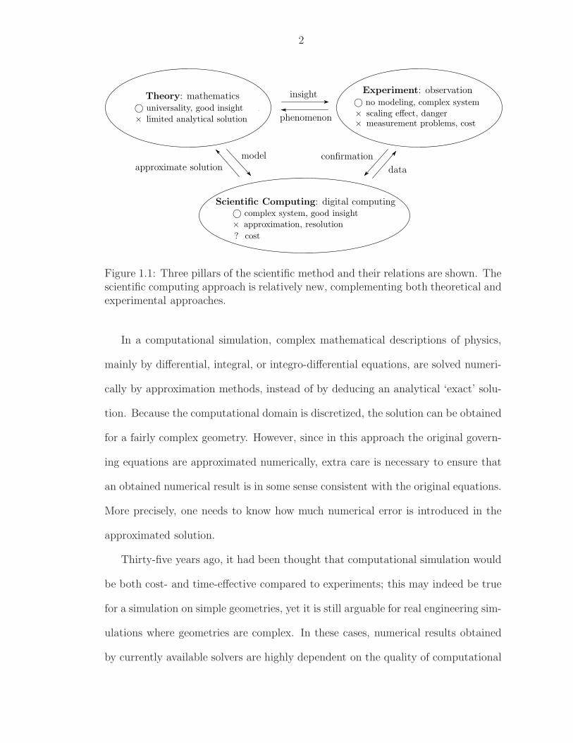
1.1 Three pillars of the scientific method and their relations are shown.The scientific computing approach is relatively new, complementingboth theoretical and experimental approaches. . . . . . . . . . . . 2
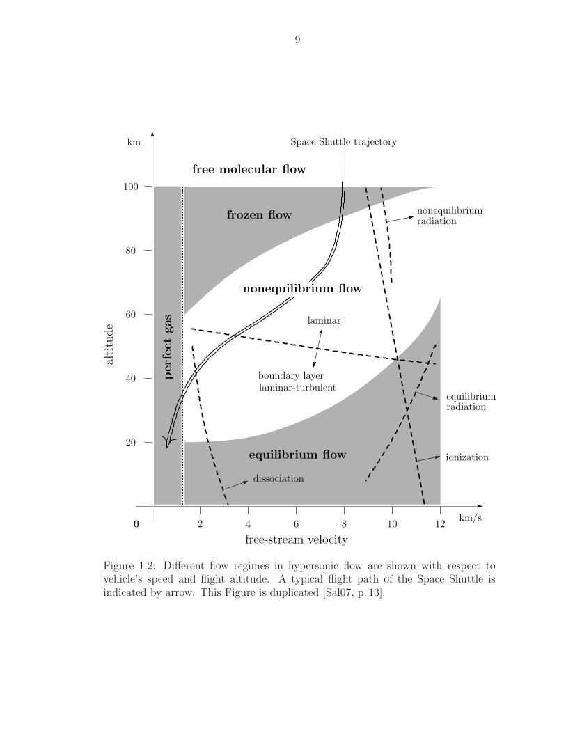
1.2 Different flow regimes in hypersonic flow are shown with respect tovehicle’s speed and flight altitude. A typical flight path of the SpaceShuttle is indicated by arrow. This Figure is duplicated [Sal07, p. 13]. 9
2.1 The development of the Hancock time integration is motivated bythe fact that when a Riemann flux is evaluated at the half timestep tn+1/2, then there is no wave interaction at both interfacesalong (xj±1/2, [t
n, tn+1/2]). Hence, predicted values associated to thehalf-time can be obtained by any form of equations, e.g., the con-servation, or primitive form, expressed in the cell’s interior. Theseequations then produce the input values for the Riemann problemsat (xj±1/2, t
n+1/2). . . . . . . . . . . . . . . . . . . . . . . . . . . . 31
2.2 Solution distribution of a DG-P 1 method (a) and the first-orderfinite volume method (b) are compared. Dashed lines in (b) arereconstructed piecewise linear distributions of a second-order finitevolume method. . . . . . . . . . . . . . . . . . . . . . . . . . . . . 35
2.3 The locations of quadrature points for the volume integral of theflux and source terms are shown in the space-time domain, [xj−1/2, xj+1/2]×[tn, tn+1]. Corresponding locations where wave interactions occurby a Riemann solver are also presented. Both Gauss–Radau andGauss–Lobatto quadratures require two Riemann fluxes at each in-terface, and one intermediate stage at either tn+1/3 or tn+1/2. In thisthesis, the Gauss–Lobatto quadrature is only used for hyperbolicconservation laws, therefore, Figure (b), does not contain quadra-ture points (©) for the source term. . . . . . . . . . . . . . . . . . 40
x
2.4 Schematic of the sequence of the discontinuous Galerkin approxi-mation to solve an original partial differential equation. The analyt-ical solution u(x, t) is projected to the finite dimensional subspaceWh(Ωh), then further decomposed to local elements. Defining thespace of polynomial functions P k(K), where K ∈ Ωh, independentlyin each element with possible discontinuity along edges, allows usto recast the global problem as the union of local problems. . . . 51
2.5 The hierarchy of discretization methodologies is shown. The Ritz–Galerkin methods can be subdivided into two methodologies: weightedresidual and Rayleigh–Ritz. Depending on the definition of testfunctions, various schemes can be distinguished. Also, various time-integration methods besides a typical ODE solver are listed. . . . 53
2.6 The surface integral of the element-interface flux over the domainei,Kj
× [tn, tn+1] is replaced by the two-point Gauss quadrature inspace. The quadrature points are denoted by bullets (•, integra-tion over [tn, tn+1]), and triangles (N, integration over [tn, tn+1/3]).At each point, a Riemann solver is applied to compute a uniqueinterface flux. . . . . . . . . . . . . . . . . . . . . . . . . . . . . . 67
2.7 The bullet symbol (•) denotes quadrature points where a Riemannflux is computed. For a P 1 method, two Riemann fluxes in theGauss points along the edge ej are required to approximate an ac-tual distribution of the interface flux with a polynomial of degreethree (cubic function). . . . . . . . . . . . . . . . . . . . . . . . . 68
2.8 The quadrature points required for the volume integrals of flux andsource term are denoted as bullet (•) and triangle (N) respectively.For the flux integration, four points are necessary at each time levelfor a quadrilateral element (a), while three points along edges arerequired for a triangular element (b). Alternative quadrature pointsfor a quadrilateral element are shown in (c), with the benefit thatconserved quantities at the Gauss points along edges are alreadycomputed when a Riemann flux has to be calculated. . . . . . . . 74
2.9 Quadrature points for Hancock’s original method. The bullet sym-bol (•) denotes quadrature points where a Riemann flux is com-puted. The midpoint rule guarantees the second-order approxima-tion of the surface integral of the flux along the edge ej . . . . . . . 82
3.1 Contour plot of the modulus of the amplification factor, |g1st-order(ν, β)|,computed with the upwind flux. It shows that the first-order methodis stable for ν ≤ 1. . . . . . . . . . . . . . . . . . . . . . . . . . . 103
3.2 Contour plot of the modulus of the amplification factor, |g1st-order(ν, β)|,computed with the Lax–Friedrichs flux. It shows that the first-ordermethod is stable for ν ≤ 1. . . . . . . . . . . . . . . . . . . . . . . 103
xi
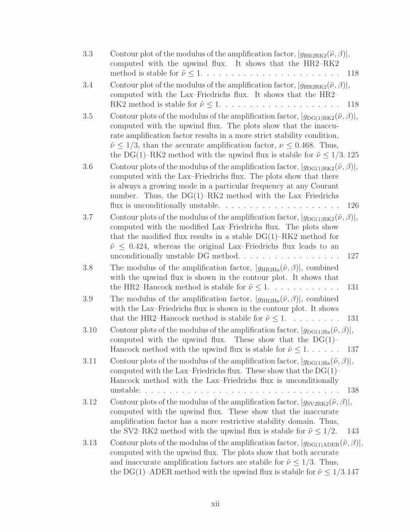
3.3 Contour plot of the modulus of the amplification factor, |gHR2RK2(ν, β)|,computed with the upwind flux. It shows that the HR2–RK2method is stable for ν ≤ 1. . . . . . . . . . . . . . . . . . . . . . . 118
3.4 Contour plot of the modulus of the amplification factor, |gHR2RK2(ν, β)|,computed with the Lax–Friedrichs flux. It shows that the HR2–RK2 method is stable for ν ≤ 1. . . . . . . . . . . . . . . . . . . . 118
3.5 Contour plots of the modulus of the amplification factor, |gDG(1)RK2(ν, β)|,computed with the upwind flux. The plots show that the inaccu-rate amplification factor results in a more strict stability condition,ν ≤ 1/3, than the accurate amplification factor, ν ≤ 0.468. Thus,the DG(1)–RK2 method with the upwind flux is stabile for ν ≤ 1/3. 125
3.6 Contour plots of the modulus of the amplification factor, |gDG(1)RK2(ν, β)|,computed with the Lax–Friedrichs flux. The plots show that thereis always a growing mode in a particular frequency at any Courantnumber. Thus, the DG(1)–RK2 method with the Lax–Friedrichsflux is unconditionally unstable. . . . . . . . . . . . . . . . . . . . 126
3.7 Contour plots of the modulus of the amplification factor, |gDG(1)RK2(ν, β)|,computed with the modified Lax–Friedrichs flux. The plots showthat the modified flux results in a stable DG(1)–RK2 method forν ≤ 0.424, whereas the original Lax–Friedrichs flux leads to anunconditionally unstable DG method. . . . . . . . . . . . . . . . . 127
3.8 The modulus of the amplification factor, |gHR2Ha(ν, β)|, combinedwith the upwind flux is shown in the contour plot. It shows thatthe HR2–Hancock method is stabile for ν ≤ 1. . . . . . . . . . . . 131
3.9 The modulus of the amplification factor, |gHR2Ha(ν, β)|, combinedwith the Lax–Friedrichs flux is shown in the contour plot. It showsthat the HR2–Hancock method is stabile for ν ≤ 1. . . . . . . . . 131
3.10 Contour plots of the modulus of the amplification factor, |gDG(1)Ha(ν, β)|,computed with the upwind flux. These show that the DG(1)–Hancock method with the upwind flux is stable for ν ≤ 1. . . . . . 137
3.11 Contour plots of the modulus of the amplification factor, |gDG(1)Ha(ν, β)|,computed with the Lax–Friedrichs flux. These show that the DG(1)–Hancock method with the Lax–Friedrichs flux is unconditionallyunstable. . . . . . . . . . . . . . . . . . . . . . . . . . . . . . . . . 138
3.12 Contour plots of the modulus of the amplification factor, |gSV2RK2(ν, β)|,computed with the upwind flux. These show that the inaccurateamplification factor has a more restrictive stability domain. Thus,the SV2–RK2 method with the upwind flux is stabile for ν ≤ 1/2. 143
3.13 Contour plots of the modulus of the amplification factor, |gDG(1)ADER(ν, β)|,computed with the upwind flux. The plots show that both accurateand inaccurate amplification factors are stabile for ν ≤ 1/3. Thus,the DG(1)–ADER method with the upwind flux is stabile for ν ≤ 1/3.147
xii
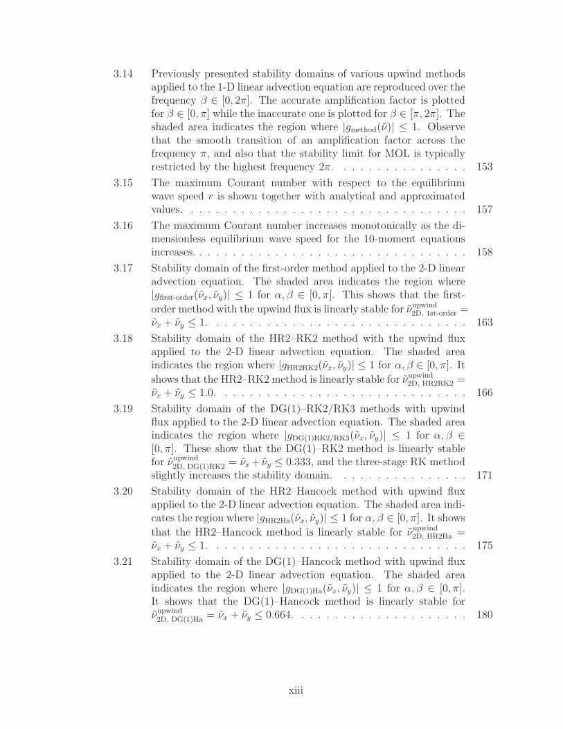
3.14 Previously presented stability domains of various upwind methodsapplied to the 1-D linear advection equation are reproduced over thefrequency β ∈ [0, 2π]. The accurate amplification factor is plottedfor β ∈ [0, π] while the inaccurate one is plotted for β ∈ [π, 2π]. Theshaded area indicates the region where |gmethod(ν)| ≤ 1. Observethat the smooth transition of an amplification factor across thefrequency π, and also that the stability limit for MOL is typicallyrestricted by the highest frequency 2π. . . . . . . . . . . . . . . . 153
3.15 The maximum Courant number with respect to the equilibriumwave speed r is shown together with analytical and approximatedvalues. . . . . . . . . . . . . . . . . . . . . . . . . . . . . . . . . . 157
3.16 The maximum Courant number increases monotonically as the di-mensionless equilibrium wave speed for the 10-moment equationsincreases. . . . . . . . . . . . . . . . . . . . . . . . . . . . . . . . . 158
3.17 Stability domain of the first-order method applied to the 2-D linearadvection equation. The shaded area indicates the region where|gfirst-order(νx, νy)| ≤ 1 for α, β ∈ [0, π]. This shows that the first-
order method with the upwind flux is linearly stable for νupwind2D, 1st-order =
νx + νy ≤ 1. . . . . . . . . . . . . . . . . . . . . . . . . . . . . . . 163
3.18 Stability domain of the HR2–RK2 method with the upwind fluxapplied to the 2-D linear advection equation. The shaded areaindicates the region where |gHR2RK2(νx, νy)| ≤ 1 for α, β ∈ [0, π]. It
shows that the HR2–RK2 method is linearly stable for νupwind2D, HR2RK2 =
νx + νy ≤ 1.0. . . . . . . . . . . . . . . . . . . . . . . . . . . . . . 166
3.19 Stability domain of the DG(1)–RK2/RK3 methods with upwindflux applied to the 2-D linear advection equation. The shaded areaindicates the region where |gDG(1)RK2/RK3(νx, νy)| ≤ 1 for α, β ∈[0, π]. These show that the DG(1)–RK2 method is linearly stablefor νupwind
2D, DG(1)RK2 = νx + νy ≤ 0.333, and the three-stage RK methodslightly increases the stability domain. . . . . . . . . . . . . . . . 171
3.20 Stability domain of the HR2–Hancock method with upwind fluxapplied to the 2-D linear advection equation. The shaded area indi-cates the region where |gHR2Ha(νx, νy)| ≤ 1 for α, β ∈ [0, π]. It shows
that the HR2–Hancock method is linearly stable for νupwind2D, HR2Ha =
νx + νy ≤ 1. . . . . . . . . . . . . . . . . . . . . . . . . . . . . . . 175
3.21 Stability domain of the DG(1)–Hancock method with upwind fluxapplied to the 2-D linear advection equation. The shaded areaindicates the region where |gDG(1)Ha(νx, νy)| ≤ 1 for α, β ∈ [0, π].It shows that the DG(1)–Hancock method is linearly stable forνupwind
2D, DG(1)Ha = νx + νy ≤ 0.664. . . . . . . . . . . . . . . . . . . . . 180
xiii
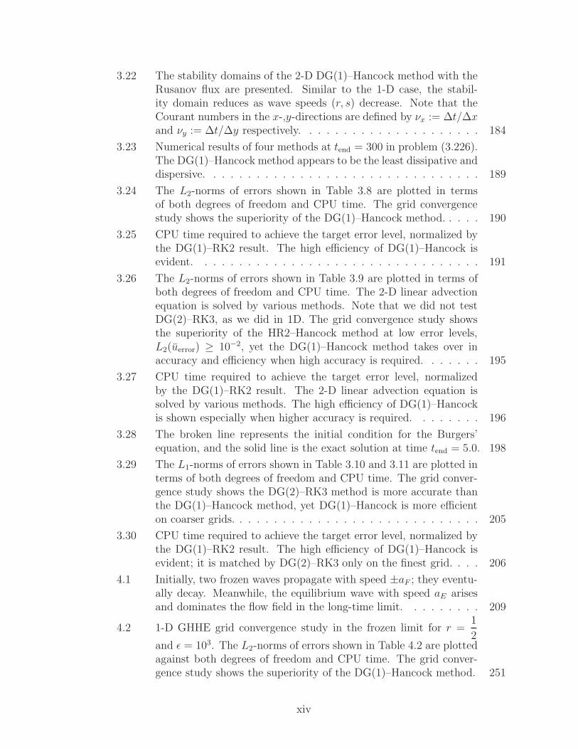
3.22 The stability domains of the 2-D DG(1)–Hancock method with theRusanov flux are presented. Similar to the 1-D case, the stabil-ity domain reduces as wave speeds (r, s) decrease. Note that theCourant numbers in the x-,y-directions are defined by νx := ∆t/∆xand νy := ∆t/∆y respectively. . . . . . . . . . . . . . . . . . . . . 184
3.23 Numerical results of four methods at tend = 300 in problem (3.226).The DG(1)–Hancock method appears to be the least dissipative anddispersive. . . . . . . . . . . . . . . . . . . . . . . . . . . . . . . . 189
3.24 The L2-norms of errors shown in Table 3.8 are plotted in termsof both degrees of freedom and CPU time. The grid convergencestudy shows the superiority of the DG(1)–Hancock method. . . . . 190
3.25 CPU time required to achieve the target error level, normalized bythe DG(1)–RK2 result. The high efficiency of DG(1)–Hancock isevident. . . . . . . . . . . . . . . . . . . . . . . . . . . . . . . . . 191
3.26 The L2-norms of errors shown in Table 3.9 are plotted in terms ofboth degrees of freedom and CPU time. The 2-D linear advectionequation is solved by various methods. Note that we did not testDG(2)–RK3, as we did in 1D. The grid convergence study showsthe superiority of the HR2–Hancock method at low error levels,L2(uerror) ≥ 10−2, yet the DG(1)–Hancock method takes over inaccuracy and efficiency when high accuracy is required. . . . . . . 195
3.27 CPU time required to achieve the target error level, normalizedby the DG(1)–RK2 result. The 2-D linear advection equation issolved by various methods. The high efficiency of DG(1)–Hancockis shown especially when higher accuracy is required. . . . . . . . 196
3.28 The broken line represents the initial condition for the Burgers’equation, and the solid line is the exact solution at time tend = 5.0. 198
3.29 The L1-norms of errors shown in Table 3.10 and 3.11 are plotted interms of both degrees of freedom and CPU time. The grid conver-gence study shows the DG(2)–RK3 method is more accurate thanthe DG(1)–Hancock method, yet DG(1)–Hancock is more efficienton coarser grids. . . . . . . . . . . . . . . . . . . . . . . . . . . . . 205
3.30 CPU time required to achieve the target error level, normalized bythe DG(1)–RK2 result. The high efficiency of DG(1)–Hancock isevident; it is matched by DG(2)–RK3 only on the finest grid. . . . 206
4.1 Initially, two frozen waves propagate with speed ±aF ; they eventu-ally decay. Meanwhile, the equilibrium wave with speed aE arisesand dominates the flow field in the long-time limit. . . . . . . . . 209
4.2 1-D GHHE grid convergence study in the frozen limit for r =1
2and ǫ = 103. The L2-norms of errors shown in Table 4.2 are plottedagainst both degrees of freedom and CPU time. The grid conver-gence study shows the superiority of the DG(1)–Hancock method. 251
xiv
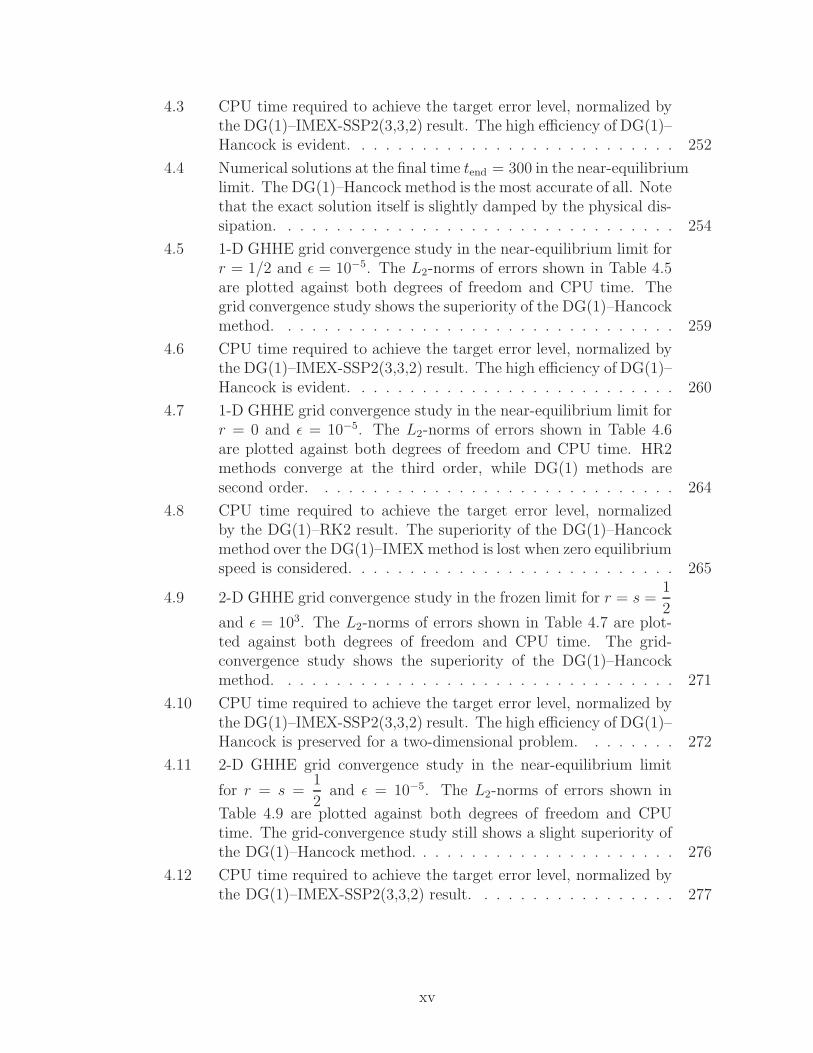
4.3 CPU time required to achieve the target error level, normalized bythe DG(1)–IMEX-SSP2(3,3,2) result. The high efficiency of DG(1)–Hancock is evident. . . . . . . . . . . . . . . . . . . . . . . . . . . 252
4.4 Numerical solutions at the final time tend = 300 in the near-equilibriumlimit. The DG(1)–Hancock method is the most accurate of all. Notethat the exact solution itself is slightly damped by the physical dis-sipation. . . . . . . . . . . . . . . . . . . . . . . . . . . . . . . . . 254
4.5 1-D GHHE grid convergence study in the near-equilibrium limit forr = 1/2 and ǫ = 10−5. The L2-norms of errors shown in Table 4.5are plotted against both degrees of freedom and CPU time. Thegrid convergence study shows the superiority of the DG(1)–Hancockmethod. . . . . . . . . . . . . . . . . . . . . . . . . . . . . . . . . 259
4.6 CPU time required to achieve the target error level, normalized bythe DG(1)–IMEX-SSP2(3,3,2) result. The high efficiency of DG(1)–Hancock is evident. . . . . . . . . . . . . . . . . . . . . . . . . . . 260
4.7 1-D GHHE grid convergence study in the near-equilibrium limit forr = 0 and ǫ = 10−5. The L2-norms of errors shown in Table 4.6are plotted against both degrees of freedom and CPU time. HR2methods converge at the third order, while DG(1) methods aresecond order. . . . . . . . . . . . . . . . . . . . . . . . . . . . . . 264
4.8 CPU time required to achieve the target error level, normalizedby the DG(1)–RK2 result. The superiority of the DG(1)–Hancockmethod over the DG(1)–IMEX method is lost when zero equilibriumspeed is considered. . . . . . . . . . . . . . . . . . . . . . . . . . . 265
4.9 2-D GHHE grid convergence study in the frozen limit for r = s =1
2and ǫ = 103. The L2-norms of errors shown in Table 4.7 are plot-ted against both degrees of freedom and CPU time. The grid-convergence study shows the superiority of the DG(1)–Hancockmethod. . . . . . . . . . . . . . . . . . . . . . . . . . . . . . . . . 271
4.10 CPU time required to achieve the target error level, normalized bythe DG(1)–IMEX-SSP2(3,3,2) result. The high efficiency of DG(1)–Hancock is preserved for a two-dimensional problem. . . . . . . . 272
4.11 2-D GHHE grid convergence study in the near-equilibrium limit
for r = s =1
2and ǫ = 10−5. The L2-norms of errors shown in
Table 4.9 are plotted against both degrees of freedom and CPUtime. The grid-convergence study still shows a slight superiority ofthe DG(1)–Hancock method. . . . . . . . . . . . . . . . . . . . . . 276
4.12 CPU time required to achieve the target error level, normalized bythe DG(1)–IMEX-SSP2(3,3,2) result. . . . . . . . . . . . . . . . . 277
xv
4.13 2-D GHHE grid convergence study in the near-equilibrium limitfor r = s = 0 and ǫ = 10−5. The L2-norms of errors shown inTable 4.10 are plotted against both degrees of freedom and CPUtime. The grid-convergence study shows all methods converge inthird-order, and error levels are comparable. . . . . . . . . . . . . 281
4.14 CPU time required to achieve the target error level, normalized bythe DG(1)–IMEX-SSP2(3,3,2) result. DG(1) methods are now lessefficient than HR2 methods due to the extra degrees of freedom.They require for achieving high accuracy. . . . . . . . . . . . . . . 282
4.15 The initial distributions of density, ρ0(x), and normalized velocity,u0(x)/a∗. . . . . . . . . . . . . . . . . . . . . . . . . . . . . . . . . 288
4.16 The density distribution at tend = 5.0, computed by the DG(1)–Hancock method, is superposed on the exact solution of the isother-mal Euler equations. . . . . . . . . . . . . . . . . . . . . . . . . . 288
4.17 L1-norms of density error, L1(ρ), for three methods are compared,showing the high accuracy of the DG(1)–Hancock method. . . . . 289
4.18 Three methods are compared regarding their overall efficiency. TheCPU time required to achieve the target error level is normalizedby the DG(1)–MOL method. The high efficiency of the DG(1)–Hancock method is observed. . . . . . . . . . . . . . . . . . . . . . 289
5.1 The original wave structure (a) is simplified to upper and lowerbounding waves plus a middle wave with speed V . Conservation isenforced in the space-time domain indicated by the dashed-line box. 299
5.2 Density distribution in steady shock structure for MU = 1.1. Thespace coordinate is normalized by the upstream mean free path λU . 304
5.3 Density distribution in steady shock structure for MU = 5.0. A“frozen” shock is followed by a relaxation zone. . . . . . . . . . . 304
5.4 The L1-norms of errors tabulated in Table 5.2 are plotted in termsof both degrees of freedom and CPU time. The grid convergencestudy shows that steady shock solutions (MU = 1.1) are secondorder accurate for HR2 and DG(1) methods. . . . . . . . . . . . . 307
5.5 Computational grid of cosine-curve nozzle. The number of cells is100×10. . . . . . . . . . . . . . . . . . . . . . . . . . . . . . . . . 308
5.6 Density profile along axis of nozzle. . . . . . . . . . . . . . . . . . 309
5.7 Ghost cells are introduced to compute gradients of flow quantities. 313
5.8 Dimensionless pressure and shear stress along the NACA0012 airfoilobtained by 10-moment and Navier–Stokes codes (Ma = 0.5, Re =5, 000, α = 0). . . . . . . . . . . . . . . . . . . . . . . . . . . . . . 316
5.9 Distribution of the dimensionless density along the centerline ofinterval x ∈ [−1, 0] is plotted. . . . . . . . . . . . . . . . . . . . . 317
xvi
5.10 Computational grid around NACA0012 micro-airfoil. The coordi-nate is normalized by the chord length. The number of cells is120 × 76. . . . . . . . . . . . . . . . . . . . . . . . . . . . . . . . . 318
5.11 Density distribution (ρ/ρ∞) around NACA 0012 micro-airfoil bythe 10-moment model, a Navier–Stokes solution, IP, DSMC meth-ods, and experiment. . . . . . . . . . . . . . . . . . . . . . . . . . 327
5.12 Dimensionless pressure and shear stress along the NACA0012 airfoilobtained by 10-moment, Navier–Stokes, and Euler codes (Ma =0.8, Re = 73, α = 0). . . . . . . . . . . . . . . . . . . . . . . . . . 328
5.13 Distribution of the dimensionless density along the centerline ofinterval x ∈ [−1, 0]. . . . . . . . . . . . . . . . . . . . . . . . . . . 329
5.14 Steady Burgers shock profile (line, exact solution cell averaged)and numerical approximation (symbols) obtained with the modifiedhyperbolic-relaxation system (5.78a); τ = 0.1, ∆x = 0.075. . . . . 334
5.15 Steady Burgers shock profile and numerical approximation obtainedwith the original hyperbolic-relaxation system (5.64a); τ = 0.1,∆x = 0.075. The numerical profile is too steep; its derivative in theorigin is infinite. . . . . . . . . . . . . . . . . . . . . . . . . . . . . 335
5.16 Grid convergence of error norms for steady-shock profiles obtainedwith the hyperbolic-relaxation system with modified source term. 336
A.1 Coordinate transformation between the global element Kj and the
local element Kj. . . . . . . . . . . . . . . . . . . . . . . . . . . . 344
A.2 A Triangular element can be subdivided into three quadrilateralelements. . . . . . . . . . . . . . . . . . . . . . . . . . . . . . . . . 347
A.3 Coordinate transformation for triangular elements. . . . . . . . . . 347
xvii
LIST OF TABLES
Table
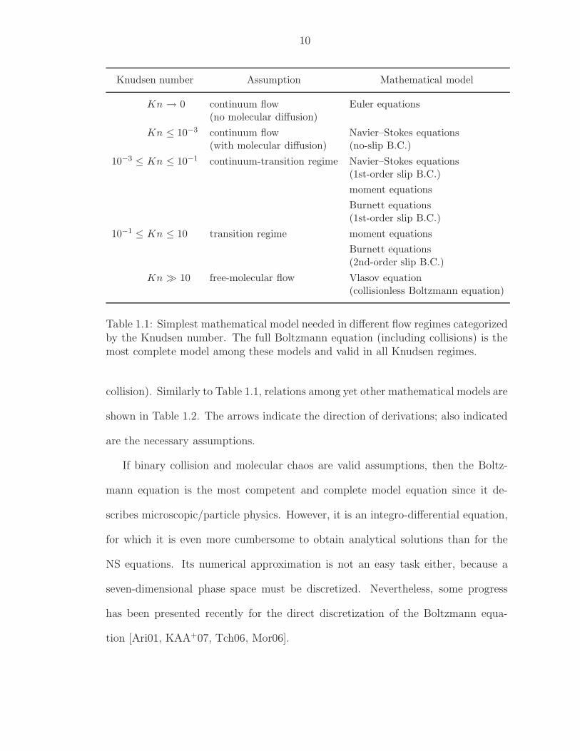
1.1 Simplest mathematical model needed in different flow regimes cate-gorized by the Knudsen number. The full Boltzmann equation (in-cluding collisions) is the most complete model among these modelsand valid in all Knudsen regimes. . . . . . . . . . . . . . . . . . . 10
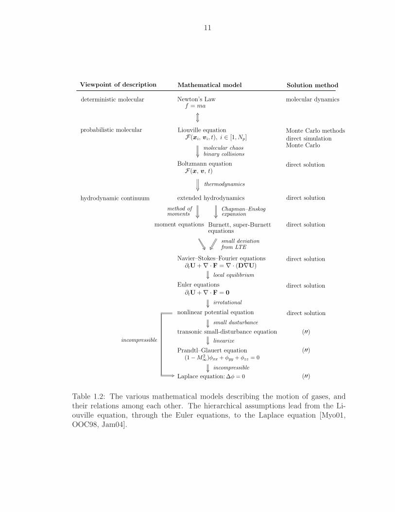
1.2 The various mathematical models describing the motion of gases,and their relations among each other. The hierarchical assumptionslead from the Liouville equation, through the Euler equations, tothe Laplace equation [Myo01, OOC98, Jam04]. . . . . . . . . . . . 11
2.1 The properties of the classes of implicit Runge–Kutta methods aretabulated [Lam91]. The order p is based on the linear theory, andthe stage order p is the lower bound obtained by the nonlineartheory. Thus, in general, the order of a method is within [p, p]. . . 42
3.1 The combinations of space and time discretization methods. Firstrow: semi-discrete methods; second row: the fully discrete methods. 89
3.2 The properties of Fourier and modified-equation analyses are sum-marized. . . . . . . . . . . . . . . . . . . . . . . . . . . . . . . . . 110
3.3 The maximum stable Courant number, νmax := r∆t
∆x, of a method
applied to the 1-D linear advection equation is tabulated. TheDG(1)–Hancock method is seen to possess the largest stability do-main among all DG discretizations listed here. . . . . . . . . . . . 151
3.4 The maximum stable Courant number, νmax := 1∆t
∆x, of a method
applied to the 1-D linear advection equation is tabulated. TheDG(1)–Hancock method reduces its stability as the equilibriumwave speed becomes smaller. If an interval is indicated, the method’sstability varies with the value of r. . . . . . . . . . . . . . . . . . . 155
xviii
3.5 The allowable maximum Courant number with respect to the equi-librium wave speed r ∈ [0, 1] for the DG(1)–Hancock method withthe Rusanov flux is tabulated. These values are measured based oncontour plots of the modulus of amplification factors. When r = 1,the result recovers the stability with the upwind flux, while the sta-bility domain is reduced towards 1/3 as the equilibrium wave getssmaller. . . . . . . . . . . . . . . . . . . . . . . . . . . . . . . . . 156
3.6 Coefficients of the polynomial approximation in (3.162). . . . . . . 157
3.7 Maximum 2-D Courant number, (ν2D)max := (νx + νy)max, for var-ious methods combined with the upwind flux (qx, qy) = (r, s) areapplied to the 2-D linear advection equation. The stability domainof DG(1)–Hancock reduces to (ν2D)max = 0.664 in two dimensions,yet greater than for DG(1)–RK2/RK3. . . . . . . . . . . . . . . . 182
3.8 A grid convergence study by solving the 1-D linear advection equa-
tion, ∂tu + r∂xu = 0 where r =1
2, is performed. The numerical
solution at tend = 300 is compared to the exact solution, then bothLp errors of u and the convergence rates are obtained for each method.188
3.9 A grid convergence study by solving the 2-D linear advection equa-
tion, ∂tu + r∂xu + s∂xu = 0 where r = s =1
2, is performed. The
numerical solution at tend = 150 is compared to the exact solution,and both Lp-errors of u and convergence rates are obtained for eachmethod. . . . . . . . . . . . . . . . . . . . . . . . . . . . . . . . . 194
3.10 A grid convergence study by solving the inviscid Burgers’ equation∂tu + u∂xu = 0. The numerical solution at tend = 5.0 is comparedto the exact solution, then both Lp-norms of error uerror and con-vergence rates are obtained for various methods. . . . . . . . . . . 202
3.11 A grid convergence study by solving the inviscid Burgers’ equation∂tu + u∂xu = 0. DG(1)–Hancock methods with various volume-integral methods are compared. The results show that doing spatialquadrature first, temporal quadrature later leads to higher accuracythan vice versa. . . . . . . . . . . . . . . . . . . . . . . . . . . . . 204
4.1 The reduced forms of the GHHE are listed in each limit. Thecharacteristic of the GHHE changes with the time scale of interest. 211
4.2 A grid convergence study by solving the 1-D GHHE in the frozenlimit (r = 1/2, ǫ = 103) is performed. L2, L∞-norms, rates ofconvergence, and CPU times of each method are tabulated. . . . . 250
4.3 L2- and L∞-norms of the exact solution at tend = 300. . . . . . . . 255
4.4 The threshold number of meshes N∗x := 1/∆h∗ of each method in
the near-equilibrium limit ǫ = 10−5 with the wave number k = 2π.The DG(1)–Hancock method requires the fewest meshes to ensurethat the physical dissipation is dominant. . . . . . . . . . . . . . . 255
xix
4.5 A grid convergence study by solving the 1-D GHHE in the near-equilibrium limit (r = 1/2, ǫ = 10−5) is performed. L2, L∞-norms,rates of convergence, and CPU times of each method are tabulated. 258
4.6 A grid convergence study by solving the 1-D GHHE in the near-equilibrium limit (r = 0, ǫ = 10−5) is performed. L2, L∞-norms,rates of convergence, and CPU times of each method are tabulated. 263
4.7 L2-, L∞-norms and rates of convergence for r = s =1
2in the frozen
limit (ǫ = 103) for the 2-D GHHE system. . . . . . . . . . . . . . 270
4.8 The threshold number of meshes N∗x := 1/∆h∗ of each method in
the near-equilibrium limit ǫ = 10−5 with wave number kx = ky = 2π. 273
4.9 L2-, L∞-norms and rates of convergence for r =1
2in the near-
equilibrium limit (ǫ = 10−5) for the 2-D GHHE system. . . . . . . 275
4.10 L2-, L∞-norms and rates of convergence for r = s = 0 in the near-equilibrium limit (ǫ = 10−5) for the 2-D GHHE system. . . . . . . 280
5.1 Initial conditions and problem setup for each test. . . . . . . . . . 303
5.2 A grid convergence study is performed by solving the 10-momentequations. L1-, L∞-norms and rates of convergence for steady shocksolutions (MU = 1.1) are computed. . . . . . . . . . . . . . . . . . 306
5.3 Reservoir condition for the nozzle flow . . . . . . . . . . . . . . . 308
5.4 Free stream condition for airfoil flow. . . . . . . . . . . . . . . . . 310
5.5 Free-stream conditions for micro-airfoil flow. . . . . . . . . . . . . 318
xx
LIST OF APPENDICES
Appendix
A. Implementation of Coordinate Transformations . . . . . . . . . . . . 343
A.1 Quadrilateral Elements . . . . . . . . . . . . . . . . . . . . 343A.2 Triangular Elements . . . . . . . . . . . . . . . . . . . . . . 346
B. Fourier Analysis of High-Order Methods . . . . . . . . . . . . . . . . 349
B.1 HR3–RK3 method . . . . . . . . . . . . . . . . . . . . . . . 349B.2 DG(2)–RK3 method . . . . . . . . . . . . . . . . . . . . . . 350B.3 DG(2)–ADER method . . . . . . . . . . . . . . . . . . . . . 352
C. Asymptotic Expansion of Dimensionless GHHE . . . . . . . . . . . . 354
C.1 One-Dimensional Systems . . . . . . . . . . . . . . . . . . . 354C.2 Two-Dimensional Systems . . . . . . . . . . . . . . . . . . . 356
D. Jin–Levermore’s Semi-Discrete High-Resolution Godunov Method . 357
E. Dispersion Analysis for the 2-D GHHE . . . . . . . . . . . . . . . . 360
xxi
ABSTRACT
This dissertation presents a step towards high-order methods for continuum-transition
flows. In order to achieve maximum accuracy and efficiency for numerical methods
on a distorted mesh, it is desirable that both governing equations and correspond-
ing numerical methods are in some sense compact. We argue our preference for
a physical model described solely by first-order partial differential equations called
hyperbolic-relaxation equations, and, among various numerical methods, for the dis-
continuous Galerkin method. Hyperbolic-relaxation equations can be generated as
moments of the Boltzmann equation and can describe continuum-transition flows.
Two challenging properties of hyperbolic-relaxation equations are the presence
of a stiff source term, which drives the system towards equilibrium, and the ac-
companying change of eigenstructure. The first issue can be solved by an implicit
treatment of the source term. To cope with the second difficulty, we develop a
space-time discontinuous Galerkin method, based on Huynh’s “upwind moment
scheme.” It is called the DG(1)–Hancock method.
The DG(1)–Hancock method for one- and two-dimensional meshes is described,
and Fourier analyses for both linear advection and linear hyperbolic-relaxation equa-
tions are conducted. The analyses show that the DG(1)–Hancock method is not
only accurate but efficient in terms of turnaround time in comparison to other semi-
and fully discrete finite-volume and discontinuous Galerkin methods. Numerical
tests confirm the analyses, and also show the properties are preserved for nonlinear
xxii
equations; the efficiency is superior by an order of magnitude.
Subsequently, discontinuous Galerkin and finite-volume spatial discretizations
are applied to more practical equations, in particular, to the set of 10-moment equa-
tions, which are gas dynamics equations that include a full pressure/temperature
tensor among the flow variables. Results for flow around a micro-airfoil are com-
pared to experimental data and to solutions obtained with a Navier–Stokes code,
and with particle-based methods. While numerical solutions in the continuum
regime for both the 10-moment and Navier–Stokes equations are similar, clear differ-
ences are found in the continuum-transition regime, especially near the stagnation
point, where the Navier–Stokes code, even when implemented with wall-slip, over-
estimates the density.
xxiii
CHAPTER I
INTRODUCTION
1.1 Motivation
In the design process, engineers need the resultant performance of devices in-
stantaneously to optimize and finalize the design. This is necessary, especially in
industry, to shorten the design process. In general, one can conduct a theoretical or
experimental analysis to understand the physics and the sources of loss in desired
performance. A theoretical analysis is a strong method owing to its universality,
however, it can not be applied to real engineering problems because of the generally
simple assumptions made. Conversely, experimental analysis is case dependent, yet
it allows testing of a reasonably complex system. The drawbacks of the experiment
are that it is often expensive and time consuming, especially if a parameter study
is necessary to optimize a design.
To overcome the limitations of both theoretical and experimental analysis, the
approach of computational simulation was introduced. Originally the complement
of theoretical analysis, it is now been recognized as a third mode of science. In
this context, computational simulation is referred to as scientific computing, or
computational science. Figure 1.1 shows the relations among these three approaches;
each approach has its own strength and weakness.
1
2
Theory: mathematics
× limited analytical solution
© universality, good insight
Experiment: observation
× scaling effect, danger
© no modeling, complex system
Scientific Computing: digital computing
× approximation, resolution
? cost
© complex system, good insight
phenomenon
insight
model confirmation
dataapproximate solution
× measurement problems, cost
Figure 1.1: Three pillars of the scientific method and their relations are shown. Thescientific computing approach is relatively new, complementing both theoretical andexperimental approaches.
In a computational simulation, complex mathematical descriptions of physics,
mainly by differential, integral, or integro-differential equations, are solved numeri-
cally by approximation methods, instead of by deducing an analytical ‘exact’ solu-
tion. Because the computational domain is discretized, the solution can be obtained
for a fairly complex geometry. However, since in this approach the original govern-
ing equations are approximated numerically, extra care is necessary to ensure that
an obtained numerical result is in some sense consistent with the original equations.
More precisely, one needs to know how much numerical error is introduced in the
approximated solution.
Thirty-five years ago, it had been thought that computational simulation would
be both cost- and time-effective compared to experiments; this may indeed be true
for a simulation on simple geometries, yet it is still arguable for real engineering sim-
ulations where geometries are complex. In these cases, numerical results obtained
by currently available solvers are highly dependent on the quality of computational
3
grids. Expertise of grid generation is necessary to generate grids ‘smooth’ enough
to accommodate deficiencies of solvers. This process may result in a duration of a
few weeks or even a month to generate a computational grid.
It is now recognized that the experiment can never be neglected; it may serve,
for instance, to validate the design of a few final candidates based on numerical
simulations.
The generality, versatility, and manageable cost of computational simulation
have lead to its heavy use in the past three decades as an analysis tool to assist
engineers with design.
‘Efficiency’ is an important concept in computational simulation. Here, we ex-
clude the pre-process (grid generation) and post-process (visualization) from con-
sideration. Under this assumption, efficiency can be decomposed into two major
factors: speed, i.e., CPU time to complete the calculation up to a given evolution
time tend on a given grid, and the numerical accuracy of the resultant numerical
solution. Therefore, efficiency can be defined as:
the total CPU time needed to yield a given solution accuracy.
This is a useful index, especially when comparing methods with different orders
of convergence. Here, the order of convergence is defined in regard to the local
truncation error of the method. If
truncation error ∼ O(∆xr, ∆ts) , (1.1)
where ∆x and ∆t are the size of discretization intervals in space and time, the
method is said to be r-th order in space and s-th order in time. A low-order
method tends to be computationally less expensive, requiring less CPU time, than
a high-order method per computational grid or time step. However, it requires finer
4
grids to reduce the truncation error to a desirable level. Thus, to achieve a pre-set
accuracy, the overall run-time of a low-order method might be longer than that
of a high-order method. This becomes more significant once a multidimensional
problem is considered. One caution we need to observe is that the order of accuracy
as defined about is not everything. Indeed, the actual truncation error is expressed
by
truncation error = C × (∆xr, ∆ts) + higher-order error, (1.2)
where C is the coefficient of the lowest-order numerical error. Thus, the magnitude
of the coefficient, C, is as important as the order of a numerical method. An
interesting discussion of this issue can be found in [LeV02, p. 150].
The efficiency index is based on the user’s point of view; if one wants to obtain
a numerical result within a particular error margin, then what method provides
the result in the shortest run-time? Here, the emphasis is not on the order of
convergence itself, but on efficiency, which indeed demonstrates how ‘good’ a method
is. Nevertheless, it has been observed that there is a high correlation between
efficiency and the order of convergence: a higher-order method tends to be more
efficient [VAKJ03, Bon99]. Besides the efficiency of a method in terms of turnaround
time, it is critical, as mentioned previously, to consider the method’s capability of
handling complex geometries. If a method is incapable of producing accurate results
on the mediocre-quality grids provided by grid-generation software packages, a vast
amount of time needs to be spent on improving the grid properties even before
starting a calculation.
In the aerospace engineering community, the compressible Navier–Stokes (NS)
equations have been adopted as the model equations to understand and analyze flow
phenomena theoretically. Due to the nonlinearity and complexity of the equations,
5
analytical solutions are only available in special cases [Whi91]. This limitation of
theoretical analysis, and the advent of the modern digital computer have motivated
scientists and engineers to solve the NS equations numerically. As a result, numer-
ous methods have been proposed for almost half a century, and great successes have
been achieved. Nowadays, computational fluid dynamics (CFD) has become one of
the most important design tools for aerospace engineers besides wind-tunnel exper-
iments. Some historical perspectives of the development of CFD in the aerospace
community, and the current status, can be bound in [Jam01, Fuj05]. Unfortunately,
there is a general consensus in the community that CFD is mature/solved, and not
much space is left for the development of an innovative numerical method. This is
somewhat understandable: the currently available methods are fairly accurate and
robust in engineering applications, and if their efficiency is not sufficient, then one
can always utilize adaptive mesh refinement to increase resolution where needed, and
implement the multigrid methods or brute-force parallelization to reduce run-time.
The ceaseless advancement of computer architectures also discourages researchers
to invest their time in developing a new numerical method. Frankly, it becomes
more and more difficult and risky to devote one’s career to inventing a method
that would appeal to other researchers and engineers, but would force them to
rewrite their in-house Euler or Navier–Stokes codes. A further discussion regarding
the stagnation of method development in the ’90s, and some unsolved problems of
current methods are presented by Roe [Roe05a].
Even though the currently available methods provide reasonably accurate re-
sults, these methods are not necessary efficient. Also, it is well-known that, on
greatly distorted grids, these methods show at most second-order convergence in
space for practical applications. The demand of solving realistic/practical prob-
6
lems translates into the use of unstructured grids, and efficient implementation on
parallel computers. The local-preconditioning [vLLR91, Tur99, RNK02] and multi-
grid-relaxation techniques [Jam91] have been developed to accelerate the conver-
gence to steady solutions; however, the benefits are still limited, and, furthermore,
applying these techniques to parallel computers is not trivial. Recently, a success
in computing steady Euler solutions with N unknowns in O(N) operations was
achieved [vLD99, NvL03]; for the Navier–Stokes equations such progress is still far
away [DvL03, KvLW05].
Because of the lack of efforts to develop new, efficient high-order methods, CFD
users have remained using classical methods, and heavily rely on parallel computing.
After a recession in method development lasting almost a decade, the need for
efficient and robust discretizations for high-fidelity CFD on unstructured grids has
become widely recognized in recent years [DH05, Wan07, Eka05]. In keeping with
this insight, we propose in this dissertation a combination of two approaches toward
efficient and robust schemes for advection-dominated flows on unstructured grids,
one at the partial-differential-equation (PDE) level and the other at the discretiza-
tion level. Specifically, we aim to develop a unified numerical method for simulating
continuum and transitional flow. This can be achieved by simultaneously taking
the following two approaches: the use of first-order PDEs and the use of compact
high-order discretizations. These will be highlighted in the next two sections.
1.2 First Approach: First-Order PDEs
The first approach is replacing everybody’s favorite Navier–Stokes equations by
a larger set of first-order hyperbolic-relaxation PDEs, which contains the NS equa-
tions. (N.B.: here ‘first-order’ refers to the order of the PDEs.) This is a rather
7
radical approach. First-order hyperbolic-relaxation equations for transitional flow
can be derived by taking moments of the Boltzmann equation. From a numeri-
cal point of view, the loss of accuracy inherent in adopting the NS equations as
the model equations is linked to the second-order derivative modeling molecular
diffusion. The elliptic nature of this term yields global data dependence on the
discretized domain, and causes a loss of accuracy on nonsmooth adaptively-refined
grids. In comparison, a first-order PDE model offers many numerical advantages,
including the following:
1. it can replace global stiffness from diffusion terms with local stiffness from
source terms, and yield the best accuracy on nonsmooth, adaptively refined
grids [CP95];
2. it requires smaller discrete stencils, reducing communications in parallel pro-
cessing;
3. it has the form of the moment closures of the Boltzmann equation, where the
source term describes departure from local thermodynamic equilibrium.
The NS equations are only valid in the continuum-fluid regime where the macro-
scopic representation of the gas is sufficient. First-order PDEs may overcome this
physical limitation. The dimensionless number that indicates whether the contin-
uum assumption is valid or not, is the Knudsen number, denoted by Kn. The
Knudsen number is defined as the ration of molecular mean free path to character-
istic length scale, thus
Kn :=molecular mean free path
characteristic length scale=
λ
L. (1.3)
8
Introducing the Mach number, Ma, and the Reynolds number, Re, and using kinetic
theory, the Knudsen number is found to have the following relation to these [GeH99]:
Kn ∼ Ma
Re. (1.4)
Hence, high Mach number or low Reynolds number lead to high Knudsen number,
resulting in a regime where the continuum assumption is no longer valid. For in-
stance, flow in or around micro-electro-mechanical systems (MEMS) or a reentry
vehicle are typically in the so-called transition regime; the flow is in between contin-
uum and free-molecular flow, with Knudsen numbers in the range 0.1 ≤ Kn ≤ 10.
In this regime the NS equations, even allowing for slip at a solid boundary, do not
describe the flow with sufficient accuracy. Table 1.1 summarizes the properties of
the simplest models available for a reliable description in different ranges of Knud-
sen numbers [AYB01]. Figure 1.2 is a schematic of physical regimes of hypersonic
flow. A typical Space Shuttle flight trajectory shows that a vehicle experiences
nonequilibrium flow in the large part of its flight path [Sal07].
As pointed out by Vincenti and Kruger, there may be a tendency to regard the
Boltzmann equation as the last mathematical model in the microscopic description
of gases, and its limitations are often overlooked [VK86, p. 333]. The limitations
of the Boltzmann equation become clear through its derivation from an even more
fundamental equation of motion, the Liouville equation. The Liouville equation is
a continuity equation, describing the time evolution of the N -particle distribution
function in a 6N -dimensional phase space; the Boltzmann equation deals only with
a single-particle distribution function. The Boltzmann equation can be derived from
the Liouville equation under the assumptions of binary (two-body) collisions and
molecular chaos (no correlation of initial velocities between two molecules before a
9
2 4 6 8 10 12km/s
20
40
60
80
100
km
equilibrium flow
frozen flow
nonequilibrium flow
dissociation
ionization
equilibriumradiation
nonequilibriumradiation
free molecular flow
laminar
boundary layerlaminar-turbulent
0
Space Shuttle trajectory
perf
ect
gas
free-stream velocity
alti
tude
Figure 1.2: Different flow regimes in hypersonic flow are shown with respect tovehicle’s speed and flight altitude. A typical flight path of the Space Shuttle isindicated by arrow. This Figure is duplicated [Sal07, p. 13].
10
Knudsen number Assumption Mathematical model
Kn → 0 continuum flow Euler equations(no molecular diffusion)
Kn ≤ 10−3 continuum flow Navier–Stokes equations(with molecular diffusion) (no-slip B.C.)
10−3 ≤ Kn ≤ 10−1 continuum-transition regime Navier–Stokes equations(1st-order slip B.C.)
moment equations
Burnett equations(1st-order slip B.C.)
10−1 ≤ Kn ≤ 10 transition regime moment equations
Burnett equations(2nd-order slip B.C.)
Kn ≫ 10 free-molecular flow Vlasov equation(collisionless Boltzmann equation)
Table 1.1: Simplest mathematical model needed in different flow regimes categorizedby the Knudsen number. The full Boltzmann equation (including collisions) is themost complete model among these models and valid in all Knudsen regimes.
collision). Similarly to Table 1.1, relations among yet other mathematical models are
shown in Table 1.2. The arrows indicate the direction of derivations; also indicated
are the necessary assumptions.
If binary collision and molecular chaos are valid assumptions, then the Boltz-
mann equation is the most competent and complete model equation since it de-
scribes microscopic/particle physics. However, it is an integro-differential equation,
for which it is even more cumbersome to obtain analytical solutions than for the
NS equations. Its numerical approximation is not an easy task either, because a
seven-dimensional phase space must be discretized. Nevertheless, some progress
has been presented recently for the direct discretization of the Boltzmann equa-
tion [Ari01, KAA+07, Tch06, Mor06].
11
Mathematical model Solution method
molecular dynamics
Monte Carlo methods
direct solution
direct solution
direct solution
direct solution
direct solution
Monte Carlodirect simulation
deterministic molecular Newton’s Law
probabilistic molecular Liouville equation
Boltzmann equation
hydrodynamic continuum extended hydrodynamics
Navier–Stokes–Fourier equations
Euler equations
moment equations Burnett, super-Burnettequations
f = ma
F(xi, vi, t), i ∈ [1, Np]
F(x, v, t)
∂tU + ∇ · F = ∇ · (D∇U)
∂tU + ∇ · F = 0
molecular chaos
thermodynamics
local equilibrium
Chapman–Enskogmethod ofmoments
Viewpoint of description
expansion
small deviationfrom LTE
binary collisions
irrotational
nonlinear potential equation
small dusturbance
transonic small-disturbance equation
linearize
Prandtl–Glauert equation(1 −M2
∞)φxx + φyy + φzz = 0
incompressible
Laplace equation: ∆φ = 0
incompressible
direct solution
(′′)
(′′)
(′′)
Table 1.2: The various mathematical models describing the motion of gases, andtheir relations among each other. The hierarchical assumptions lead from the Li-ouville equation, through the Euler equations, to the Laplace equation [Myo01,OOC98, Jam04].
12
To circumvent the numerical and mathematical adversities of the Boltzmann
equation, mainly two approaches have been proposed: the direct-simulation Monte
Carlo (DSMC) method [Bir63, Bir94] and extended-hydrodynamics (generalized
hydrodynamics) methods [CC70, Str05, MR98, Eu92].
The DSMC method, a particle-based method, introduces computational parti-
cles representing the bulk of actual molecules to model the translational and colli-
sional phenomena. Thus, this method does not literally solve the Liouville/Boltzmann
equation numerically, yet under the assumption of molecular chaos and binary col-
lisions, it has been proved that the DSMC method converges to the solution of
the Boltzmann equation as the number of particles tends to infinity [Wag92]. The
method is extremely accurate, especially in the high Knudsen regime. The DSMC
method is required for the highest Knudsen numbers, i.e., rarefied flow, however, in
the transition regime there is competition with extended-hydrodynamics methods.
The DSMC method produces statistical scatter in the solutions, and it requires a
cell size of the order of the molecular mean free path. These properties lead to a
computational penalty, especially in the transition (low Knudsen number) regime.
Conversely, the extended-hydrodynamics methods are PDE-based, thus they do not
have such statistical issues.
Extended-hydrodynamics methods assume the shape of the velocity-distribution
function (VDF) in the Boltzmann equation, then transform from the microscopic to
the macroscopic representation through taking moments over the velocity spaces.
Reducing the dimension of the equation by defining macroscopic quantities pro-
vides the mathematical simplicity and computational efficiency. Actually, there are
two essential approaches to deriving macroscopic governing equations: the Chap-
man–Enskog expansion and Grad’s method of moments.
13
The Chapman–Enskog expansion adopts a perturbed Maxwellian distribution
function, then the macroscopic variables are expanded with respect to the Knudsen
number as the small parameter. The advantage of the Chapman–Enskog expan-
sion is that the number of state variables stays the same as in the NS equations,
i.e., (ρ, ρu, ρE) for the conserved quantities. However, higher-order derivatives are
introduced to describe the non-equilibrium phenomena. The resulting equations
are called the Burnett [Bur36, CC70] and super-Burnett equations [WC48, Foc73,
Sha93] corresponding to the second- and third-order expansion with respect to the
Knudsen number. The Burnett equations, for instance, contain third-order deriva-
tives; these undesirable higher-order terms cause discretization issues on a nons-
mooth grid. Furthermore, the Burnett and super-Burnett equations are known to be
linearly unstable [Bob82, UVGC00]. In the augmented Burnett equations [ZMC93],
some super-Burnett terms are added to stabilize the equations. Another direction
is simplifying the collision integral via the Bhatnagar–Gross–Krook (BGK) model;
the resulting system is called the BGK–Burnett equations [AYB01, Bal04]. Despite
the efforts to improve the original Burnett equations, the higher-order terms re-
main highly undesirable with regard to discretization on nonsmooth grids. For this
reason, we have eliminated the choice of the Burnett equations or the extended-
hydrodynamics equations derived by the Chapman–Enskog expansion as the gov-
erning equations.
Grad’s method of moments utilizes a distribution function in a Hilbert space,
and takes moments over the phase space [Gra49]. The resulting equations are called
‘moment equations.’ The advantage of Grad’s method of moments is that the re-
sulting equations contain only first-order derivatives. However, now the number of
state variables, hence the number of governing equations, is increased. This would
14
seem to be a computational penalty, but these quantities actually have their ben-
efits. For instance, the heat fluxes, which form a vector in the NS equations, now
fill up a tensor, and evolution equations for these higher-order quantities exist and
are coupled to the mass and momentum equations. Similarly, all elements of the
shear stress tensor have their own evolution equation. In comparison, the NS equa-
tions employ algebraic constitutive laws for stress (Stokes) and heat flux (Fourier);
these quantities are proportional to the gradients of velocity and temperature, re-
spectively. Having the stress and heat-flux tensors evolve together with the other
conserved quantities makes one expect to obtain a more accurate prediction of these
physical quantities. Combining the representation of non-equilibrium gas dynamics
with our vision of numerical efficiency, the Grad-type method of moments appears
the most suitable approach to constructing the governing equations from the Boltz-
mann equation. Recall that describing physics solely by first derivatives is the key
to developing efficient, highly parallelizable schemes on nonsmooth grids.
Despite the promising properties of the moment equations, the level of maturity
of this approach is far from affording it to replace or complement the NS equations
and the DSMC method. Mainly, two obstacles need to be overcome to make the
approach applicable to a practical engineering problem; again one is at the PDE
level, and the other is at the discretization level.
The first issue is that, particularly for steady supersonic flow, the moment equa-
tions produce a discontinuity inside a smooth shock structure [Gra52, Hol64]. This
is due to the nature of hyperbolic equations, which allow the physical quantities
to propagate only at finite characteristic speeds. In reality, owing to the signifi-
cant effect of molecular diffusion, a smooth shock profile connects the upstream and
downstream states. This smooth profile is not realized by the moment equations
15
once a flow is above a critical Mach number. For Grad’s 13-moment equations, the
critical Mach number is approximately 1.65. Some improvements in the model have
been shown to increase the critical Mach number, e.g., by taking further higher-
moment equations [Wei95], or introducing second-order dissipation terms in the
system [TS04]. Even though making the moment approach more suitable for su-
per/hypersonic flow is a critical issue, the derivation of a new set of equations is
beyond the scope of this study. Here, we will only adopt the robust and physically
reasonable ‘10-moment equations’ [Lev96, Bro96] as a representative set of model
equations.
The second issue is the lack of an efficient numerical method. The moment equa-
tions have the form of hyperbolic equations with a relaxation source term. Since the
source term is parameterized by the ‘relaxation time’, which is of the order of the
mean collision time, any standard explicit method has a severe time-step restriction
with regard to both stability and accuracy, especially if one is only interested in
evolution at the macroscopic temporal and spatial scale. A standard implicit treat-
ment for the source term overcomes the stability restriction; however, taking the
large time step does not necessary guarantee the accuracy of solutions. This study
mainly focuses on this issue, i.e., the development of efficient and accurate methods
for hyperbolic-relaxation equations with stiff relaxation source terms.
1.3 Second Approach: Compact High-Order Method
The second approach is to adopt a high-order discretization method that can
preserve compactness in both space and time. Here, a compact method refers to
one satisfying the following property:
the update to a given cell should only be a function of the tn-solutions
16
of the cell itself, and its immediate neighbors [Low96, p. 4].
Since the methodologies to achieve high-order convergence in space and in time
differ considerably, a discretization method in space is discussed first.
1.3.1 Spatial Discretization
In a standard finite-volume method (FVM), solutions are defined as cell-averaged
quantities over the computational domain, and the higher-order accuracy in space
relies on local piecewise-polynomial reconstruction, which requires extended stencils.
Representative of the great successes achieved by higher-order FVMs are MUSCL1
(second-order in space) by Van Leer [vL79] and PPM2 (third-order in space) by
Colella and Woodward [CW84]. Later, the k-exact reconstruction was proposed by
Barth and Jespersen [BJ89]. Among these reconstruction methods, where recon-
struction stencils are fixed, a total-variation-diminishing (TVD) limiter is necessary
to ensure solution monotonicity near a discontinuity. Two defects of this approach
are the clipping of local extrema and the difficulty of extending the TVD philoso-
phy to multiple dimensions. (For a multidimensional solutions, sensing monotonic-
ity by the total variation is unsuited.) In practice, limiting is done dimension by
dimension using a one-dimensional TVD condition. The clipping of extrema can
be avoided by replacing the TVD condition by the total-variation-bounded (TVB)
condition [Shu87, CS89].
To overcome the difficulty of extending the TVD principle to multidimensional
problems, Harten et al. proposed the Essentially Non-Oscillatory (ENO) scheme,
which is TVB and retains high-order accuracy in smooth regions [HOEC86, HO87,
1The acronym for Monotone Upstream-centered Scheme for Conservation Laws.
2The acronym for Piecewise Parabolic Method.
17
HEOC87]. In brief, an ENO scheme uses adaptive stencils in order to choose the
stencil on which the solution is smoothest; this way the reconstructed polynomial
never spans a discontinuity. However, choosing the best stencil may vary erratically,
causing anomalies in the reconstructed solution. Later, a more robust reconstruction
process, based on a convex combination of interpolants on all possible stencils,
called weighted ENO (WENO) was proposed by Liu et al. [LOC94], and Jiang and
Shu [JS96]. The extension of the WENO scheme to nonsmooth grids was proposed
by Friedrichs [Fri98], and Hu and Shu [HS99]. These reconstruction techniques have
allowed higher-order spatial discretization in the finite volume framework; however,
an issue is that the higher a method’s order, the larger the reconstruction stencils
are. For instance, stencils for the quadratic reconstruction (for third-order accuracy)
on tetrahedral grids require 50 to 70 cells [DL99].
The discontinuous Galerkin (DG) method overcomes the issue of growing stencils
by increasing a solution representation in each element; a solution in a cell/element
is no longer piecewise constant, but polynomial of degree k. Obviously, when
k = 0, a DG method is equivalent to a first-order finite volume method. A DG
method was first introduced by Reed and Hill at Los Alamos National Laboratory
to solve the steady linear neutron transport equation [RH73]. Soon after, LaSaint
and Raviart presented error analyses, and showed that a DG(k) method for a steady
one-dimensional problem is of order 2k+1, and for a two-dimensional problem with
strictly rectangular elements it is of order k + 1 [LR74]. The analysis was later
extended to general triangular elements by Johnson and Pitkaranta, who showed
that the formal order of accuracy of DG(k) is k +1
2[JP86, Joh87]. The result was
confirmed numerically by Peterson [Pet91]. For a comprehensive literature review of
almost three decades of DG research, see Cockburn and Shu [CS01], and Zienkiewicz
18
et al. [ZTSP03]. Surprisingly, attention to DG methods in the aerospace commu-
nity came quite recently. Part of the reason was the robustness of second-order
finite-volume methods, and the advent of massively parallel computers in the early
’90s. These circumstances made CFD practitioners and code developers complacent.
Besides the DG spatial discretization, there are other methods that also pre-
serve the compactness while achieving high-order convergence in space on nons-
mooth grids, in particular, the spectral difference (SD) [LVW06] and spectral vol-
ume (SV) [Wan02] methods. A comparisons between the SV and DG methods was
presented in [ZS05, SW04]. The authors conclude that the DG method is more
accurate but requires more memory and has a more restrictive stability condition
than the SV method. Shu also compared high-order finite-difference, finite volume
WENO, and DG methods [Shu03]. He concludes that DG methods are the most
flexible in terms of arbitrary triangulation and boundary conditions, but the de-
velopment of more robust and high-order-preserving limiters is necessary. In this
thesis, we purposely exclude high-order finite-difference methods and spectral meth-
ods, as their applicability is limited to structured grids. Among the exceptions is
the spectral method developed by Kopriva, which can be applied to unstructured
quadrilateral staggered grids. Carpenter and Gottlieb also extended spectral meth-
ods to unstructured grids [CG96].
Another class of high-order methods called the spectral element method, origi-
nally developed by Patera [Pat84], uses high-order polynomials to achieve spectral-
like convergence. The further development of the spectral element method in the
context of a DG method was done by Karniadakis and Sherwin [KS05].
Related to the Galerkin formulation, Hermitian methods achieve high-order ac-
curacy by defining not only solutions at nodes, but their derivatives at the same
19
points. This type of element is called a Hermitian element, compared to the La-
grangean elements, which define only the solution itself, but at multiple places
in an element. Since the method adopts the Hermitian polynomials for the solu-
tion approximation, we could consider the Hermitian methods a Galerkin method,
yet it does not utilize the weighted-residual formulation completely. Due to the
continuity requirement of a certain order at each node, the method is currently
restricted to linear equations, and a main drawback is that Hermitian methods
are non-conservative [Roe05b, pp. 240–244]. Recent developments and applica-
tions of Hermitian methods to computational acoustics are presented by Capdev-
ille [Cap05, Cap06, Cap07].
1.3.2 Temporal Discretization
So far, only spatial discretization has been discussed. As to the temporal dis-
cretization, the semi-discrete method is currently the most successful approach. A
semi-discrete method incorporating the method-of-lines (MOL) [Sch91] decomposes
the spatial and temporal discretizations. This simplifies the development/formulation
of a method and its coding significantly. Once the spatial discretization is con-
structed, one’s favorite ODE solver can be employed for the time discretization.
Details of methods for ODE’s can be found in [Lam91, HNW93, HW96]. For
hyperbolic conservation laws, a TVD Runge–Kutta ODE solver is the common
choice [SO88]. More recently it is referred to as the strong stability-preserving (SSP)
method [GST01]. The methods are one-step multi-stage and assure nonlinear tem-
poral stability. One of the drawbacks of the semi-discrete approach is that the sta-
bility condition becomes increasingly restrictive as the spatial discretization method
goes higher-order. This has been observed for the DG method [CS01, p. 191] and
20
the SV method [Wan02, p. 249]. Increasing the order of the RK solver slightly re-
laxes the stability restriction; however, this introduces extra function evaluations,
making the method more expensive. Another defect of RK methods is that, if the
fifth or higher order in time is desired, the required number of stages is greater than
the order of a method; this is called the Butcher barrier [Lan98, p. 182].
Another class of ODE solvers are multi-step methods: Adams–Bashforth, Adams–
Moulton, and the backward-difference formula (BDF) et al.. A multi-step method
achieves high-order accuracy by utilizing the prior solutions, whereas a multi-stage
method does it by adding function evaluations. Thus, a multi-step method is gen-
erally less expensive, but more memory is required to store the prior solutions. Fur-
thermore, the size of the time-step is more restricted due to the data-dependence
over multiple times.
1.3.3 Space-Time Discretization
To overcome the stability restriction and lesser efficiency of the semi-discrete
MOL approach, the fully discrete method is considered. In this approach, spa-
tial and temporal operators are discretized in similar manner. The classical one
is the Lax–Wendroff method, second-order in both space and time [LW64]. The
method takes advantage of the original PDEs, replacing the temporal derivative
by spatial derivatives. To our knowledge, the first attempt to include a DG spa-
tial discretization in the space-time approach was done by Bar-Yoseph [BY89], and
Bar-Yoseph and Elata [BYE90]. They apply the space-time DG method to the
1-D Euler equations. Due to their choice of space-time mesh, their method is fully
implicit. Choe and Holsapple combine the idea of the temporal Taylor–Galerkin
method, which is a finite-element extension of the Lax–Wendroff idea, with the
21
discontinuous Galerkin method in space (they denote this as TG–DFEM: Tay-
lor–Galerkin discontinuous finite-element method). The resulting method is one
step, explicit second-order in both space and time, and stable up to a Courant
number of 0.4. The method is applied to 1-D scalar linear and nonlinear equations.
Later, Lowrie et al. develop an explicit space-time DG method, and present a super-
convergence result, O(2k + 1) convergence, in both Fourier analyses and numerical
tests [LRvL95, Low96, LRvL98]. However, the resulting method for 2-D problems
requires staggered grids, and could suffer from substantial numerical dissipation.
More recently, the idea of high-order space-time discretizations has returned to
the finite volume framework. Toro et al. developed an arbitrarily high order (ADER)
method: a one step method with modified generalized Riemann problems solved at
each cell interface [TMN01]. Later, Dumbser et al. applied the ADER approach to
the DG framework [DM05, QDS05]. Again, the method is one step, requiring the
same memory space as the forward-Euler time integration. The results show that
their DG–ADER or DG–LW method is more efficient than a DG–RK method due
to the reduced usage of a limiter at intermediate stages. However, a Fourier analysis
shows that these fully discrete methods still have a similar stability restriction as
DG–RK methods [DM06, p. 224][QDS05, p. 4533].
The approach by Van der Vegt and Van der Ven is more direct; they treat
space and time variables in the same manner, and construct a four-dimensional
discontinuous functional space to represent solutions. They denote this approach as
the space-time discontinuous Galerkin method [vdVvdV02, KvdVvdV06]. Unlike
semi-discrete methods, the method is inherently implicit, and pseudo-time stepping
is introduced to solve the implicit equations in each time interval.
Our approach is also to develop a method with complete coupling, thus discretiz-
22
ing in both space and time simultaneously. Yet, the current method still stays in
between semi-discrete and fully discrete methods since trial (basis) functions for the
solution representation solely depend on space, not on time. The method proposed
here is based on the ‘upwind moment scheme’ recently developed by Huynh for
hyperbolic conservation laws [Huy06a], and based in turn on Van Leer’s Scheme III
in [vL77, p. 281]. The solution representation is only piecewise linear. The two key
characteristics of this method are:
1. cell variables are updated over a half time step without any interactions with
neighboring cells (Hancock’s observation [vAvLR82]);
2. the gradient of each flow variable evolves by an independent equation (DG
representation).
The story behind the invention of Hancock’s scheme and its relation to MUSCL
and PPM are described in [vL06, Hol96]. The resulting scheme looks promising in
comparison to the popular MOL approach. The upwind moment scheme is a fully
discrete, one-step method with one intermediate update step needed for computing
the volume integral of the fluxes. It requires solving a Riemann problem twice at
each cell interface but achieves third-order accuracy in space and time.
In this thesis, the upwind moment method, originally developed for hyperbolic
conservation laws, is extended to hyperbolic-relaxation equations. Here, we will call
the method in a more generic manner, ‘DG(k)–Hancock method.’ The method pre-
serves compactness through a DG spatial discretization, and attains a high efficiency
by the Hancock discretization in time interlaced by a Gauss–Radau quadrature for
the source term.
23
1.4 Current State of Hyperbolic–Relaxation Equations
1.4.1 Mathematical Background
Our target equations, the moment equations, have the form of hyperbolic-
relaxation equations. More precisely, these are systems of hyperbolic equations
with stiff relaxation source terms such that
∂tu(x, t) + ∇ · f(u) =1
ǫs(u); x ∈ Ω, t > 0, (1.5)
where u, s ∈ Rm, f ∈ Rm×3, and ǫ > 0 is the relaxation time. In the above equations
there exist two time scales: one is the advective time scale denoted by T and the
other is the relaxation time ǫ. We need to keep in mind that these two time scales
are genuinely disparate. Also, the above form is somewhat more restrictive than
the general form of hyperbolic equations with stiff source terms. For instance,
advection-reaction equations have the same form as the above equations, but the
source term is not the relaxation source term. In this case, the system possesses
multiple equilibrium states, whereas the stiff relaxation source term always leads the
system to the unique equilibrium state. Here, we only consider such stiff-relaxation
source terms.
Let a be the characteristic wave speed, hence of the order of the eigenvalues of
the flux Jacobian ∂fn/∂u, and L be the characteristic length, then we have
T =L
a. (1.6)
The behavior of hyperbolic-relaxation equations dramatically changes as the ratio of
two time scales (stiffness parameter),T
ǫ, changes; the stiffness parameter is inversely
proportional to the Knudsen number. When the advection is dominant, and the
relaxation towards the equilibrium state is slow, hence T ≪ ǫ, then the systems is
24
called to be in the frozen limit. In this case, the original equations become pure
advection equations,
∂tu(x, t) + ∇ · f(u) = 0, (1.7)
which correspond to the collisionless Boltzmann equation. When wave propagation
and relaxation processes are equally important, hence T ∼ ǫ, then the state is in the
transition regime. See Table 1.1 on page 10 for the corresponding Knudsen range.
When the source-term effect dominates that of the wave propagation, T ≫ ǫ,
the system is said to be in the near-equilibrium limit. In such a regime, the original
hyperbolic-relaxation equations reduce to a system of n < m second-order equations
∂tU + ∇ · F(U) = ∇ · (D(U)∇U), (1.8)
where U ∈ Rn,F ∈ Rn×3, and D ∈ Rn×n is a tensor of diffusion coefficients, with
eigenvalues proportional to ǫ. This reduced system is derived through a Chap-
man–Enskog expansion [CLL94, Liu87], and the corresponding physical equations
are the Navier–Stokes equations. Subsequently, when ǫ → 0, the system reaches the
equilibrium limit:
∂tU + ∇ · F(U) = 0, (1.9)
and this is the form of the Euler equations. In the context of gas kinetics, the
equilibrium limit means that wherever a velocity distribution function is away from
the equilibrium (Maxwellian) distribution, the source term drives the state to the
local thermodynamic equilibrium instantaneously.
When we consider a numerical method to solve the hyperbolic-relaxation equa-
tions (1.5) in the near-equilibrium or equilibrium limit, a common explicit integra-
tion in time will result in the following restrictive time step:
∆t ∼ ǫ. (1.10)
25
In contrast, a typical explicit method for the Euler equations (1.9) leads to the time
step:
∆t ∼ ∆x
a≫ ǫ, (1.11)
where ∆x is the typical size of a computational cell. Hence, one might expect that
even though we solve the hyperbolic-relaxation equations (1.5), in the equilibrium
limit, we could construct a method with a time step ∆t ∝ ∆x. This means that
a method does not need to resolve the fast relaxation process described by the
source term, yet provides the correct equilibrium limit numerically. In general, this
property is called underresolved or asymptotic preserving. A similar argument can
be made for the Navier–Stokes equations, but the well-known restriction due to the
explicit treatment of the diffusion term leads to ∆t ∝ ∆x2. If the diffusion term is
treated implicitly, then we recover the advective time-step constraint: ∆t ∝ ∆x.
In order to develop such a method, there are two numerical issues to overcome:
maintaining stability in the stiff (near-equilibrium/equilibrium) regime, and ob-
taining the accurate reduced system numerically. The stability issue can be solved
quite easily; implicit treatment of the source terms, particularly an L-stable method,
guaranties the unconditional stability even in the stiff regime. However, a stable
numerical method for hyperbolic-relaxation equations does not always ensure that
the method simultaneously reduces to a consistent discretization of the reduced
equations. This is simply because the method does not know anything about the
reduced equations. As shown by Hittinger [Hit00], and Hittinger and Roe [HR04],
the resulting equilibrium flux F(U) is the resultant of tight coupling between the
frozen flux f(u) and the relaxation source term s(u). This becomes more clear when
the following 1-D linear hyperbolic-relaxation equations,
∂tu + A∂xu = Qu, (1.12)
26
are considered. By introducing new variables w such that u = eQ tw, they show
that the resulting finite-volume method has the form [HR99, RH01]:
un+1j = eQ∆tun
j − 1
∆x
tn+1∫
tn
eQ(tn+1−t)(fj+1/2(t) − fj−1/2(t)
)dt. (1.13)
The above equations show that when the relaxation is fast, thus Q is large, cell-
interface fluxes are a combination of the frozen flux and exponential damping.
Hence, separating the flux and source evaluations as with operator splitting fails
to capture the coupling, and results in a reduction of the order of accuracy due to
excessive numerical dissipation [LMM87, LM89, Pem93b, JL96, AR97].
The above formulation also reveals that a straightforward frozen Riemann solver
based on f(u) becomes inadequate in the near-equilibrium/equilibrium limit, where
a Riemann flux should be constructed based on the equilibrium flux F(u). Using a
‘frozen’ Riemann solver even in the near-equilibrium limit means that the numer-
ical method tries to push the system back to the frozen limit; this is completely
opposite to how the source term acts in the system. There are basically two ap-
proaches to achieve the coupling. The first approach, the ideal one but definitely
uphill, is constructing a Riemann solver with built-in source-term effect. In this
way, the eigenstructure of the Riemann solver automatically adapts from frozen to
equilibrium limit based on the parameter∆t
ǫ. Substantial work along this path has
been conducted by Pember [Pem93b, Pem93a] and Hittinger [Hit00].
The second approach is more straightforward. It was shown that the simple
operator splitting results in reducing the order of accuracy, due to insufficient cou-
pling. But we can introduce more coupling, for instance, by adding extra stages in
method-of-lines. Recently, Pareschi and Russo extended implicit-explicit (IMEX)
Runge–Kutta methods, originally developed by Ascher et al. for advection-diffusion
27
equations [ARW95, ARS97], to hyperbolic-relaxation equations [PR05]. The IMEX
Runge–Kutta methods together with the WENO spatial reconstruction result in
second- and third-order methods, and a numerical test confirms analyses.
Our approach based on a compact high-order method stays in between the above
two approaches. Due to the usage of a frozen Riemann solver, this approach does
not solve the fundamental issue described previously. However, it is well-known
that, as a method becomes higher-order, the choice of Riemann solver becomes less
important to accuracy; in this way, we circumvent the lack of an ideal Riemann
solver in the near-equilibrium/equilibrium limit by adopting a high-order method
with enough coupling between the frozen flux and the sources. A high-order method
also prevents the physical dissipation to be smeared by the numerical dissipation
on unresolved coarse grids.
In this section, we have briefly overviewed the properties of hyperbolic-relaxation
equations. The more detail mathematical descriptions and proofs can be found in
the review paper by Natalini [Nat98] and references therein. A concise description
is also provided in [LeV02, pp. 410–415].
1.4.2 Previous Work
In [HSvL05], various numerical methods for hyperbolic-relaxation equations are
categorized into the following four types:
• semi-discrete method [LMM87, LM89, JL96, LM99b, CJR97, PR05],
• characteristic method [AR97, AR98, Par98],
• central-difference finite-volume method [BS97, LRR00],
• modified coupled-space-time Godunov method [Pem93b, Hit00].
28
Recently, Lowrie and Morel developed the DG(1) spatial discretization method
together with an implicit time integrator for linear hyperbolic-relaxation equa-
tions [LM99b, LM99a, LM02]. Based on Fourier analyses and numerical tests, they
show that the DG(1) method is asymptotic preserving in their diffusion scaling.
Hence, second-order accuracy is uniformly achieved without damaged by the nu-
merical dissipation even though the relaxation process is not resolved at all. Their
promising results interested us in the potential use of DG methods for discretizing
first-order systems for compressible, viscous flow. However, the application of their
results to our problem must be done with care because their choices of scaling and
limit-taking are not the same as ours. A detailed discussion is formed in [HSvL05],
while further investigation for fully discrete methods based on Fourier analyses and
numerical tests are presented in this thesis in Chapter IV.
1.5 Outline of Thesis
This thesis is organized as follows. In Chapter 2, at first the DG(1)–Hancock
method for systems of one-dimensional hyperbolic-relaxation equations is described.
The detailed mathematical finite-element formulations are omitted for simplicity.
Once the 1-D DG(1)–Hancock method is described, the multidimensional extension
is provided in the following section together with more rigorous formulations. Be-
sides the DG(1)–Hancock method, the original Hancock method and semi-discrete
methods (ODE solvers) are also described for later comparisons. The original up-
wind moment scheme by Huynh for systems of hyperbolic conservation laws is also
described.
In Chapter 3, instead of jumping straight to the analysis for hyperbolic-relaxation
equations, the analysis of DG(1)–Hancock method for the scalar one- and two-
29
dimensional linear advection equations are performed. In these cases, the DG(1)–
Hancock method is equivalent to both Van Leer’s scheme III and Huynh’s upwind
moment scheme. The dissipation/dispersion errors, the order of accuracy, and the
stability condition are compared to those of various semi-discrete and fully discrete
methods. The numerical results presented later confirm the analyses. It is shown
that the DG(1)–Hancock method preserves the prominent properties of both finite-
volume and finite-element methods, and the stability constraint can be more relaxed
than that of semi-discrete DG–RK methods.
In Chapter 4, after understanding the basic properties of the DG(1)–Hancock
method for hyperbolic conservation laws, the analyses of the DG(1)–Hancock method
and other currently available methods for one- and two-dimensional linear hyperbolic-
relaxation equations are conducted. Again, dissipation/dispersion error, and the
order of accuracy are compared to those of various methods. The Fourier analy-
sis shows high accuracy with minimum number of Riemann solvers. The following
numerical tests confirm the analyses, and also the efficiency of the DG(1)–Hancock
method compared to several semi-discrete methods.
In Chapter 5, the methods are applied to more practical equations, in particu-
lar, the set of 10-moment equations which are gas dynamics equations that include
a pressure/temperature tensor. The external flow around a NACA0012 airfoil is
computed and compared with flow results from alternative methods: the NS equa-
tions, Information Preservation (IP) method, and DSMC; these solutions are also
compared to experimental flow measurements.
The conclusions and suggestions for future work are following in Chapter 6.
CHAPTER II
NUMERICAL METHODS FOR HYPERBOLIC
EQUATIONS WITH RELAXATION SOURCE
TERM
2.1 Introduction
The method proposed here to solve the hyperbolic-relaxation equations,
∂tu(x, t) + ∂xf(u) =1
ǫs(u); x ∈ R, t > 0, (2.1)
where u ∈ Rm, is based on the ‘upwind moment scheme’ [Huy06a] recently devel-
oped by Huynh for hyperbolic conservation laws:
∂tU(x, t) + ∂xF(U) = 0; x ∈ R, t > 0, (2.2)
where U ∈ Rn, n < m. Recall that the hyperbolic-relaxation equations we are inter-
ested in have a unique equilibrium limit; when ǫ → 0, (2.1) reduces to the hyperbolic
conservation laws (2.2). The solution representation of the upwind moment scheme
is only piecewise linear. The two key characteristics of this method are:
1. After initial gradient is established at each cell, cell variables are updated over
a half time step without any interactions with neighboring cells (Hancock’s
observation [vAvLR82, vL06]);
30
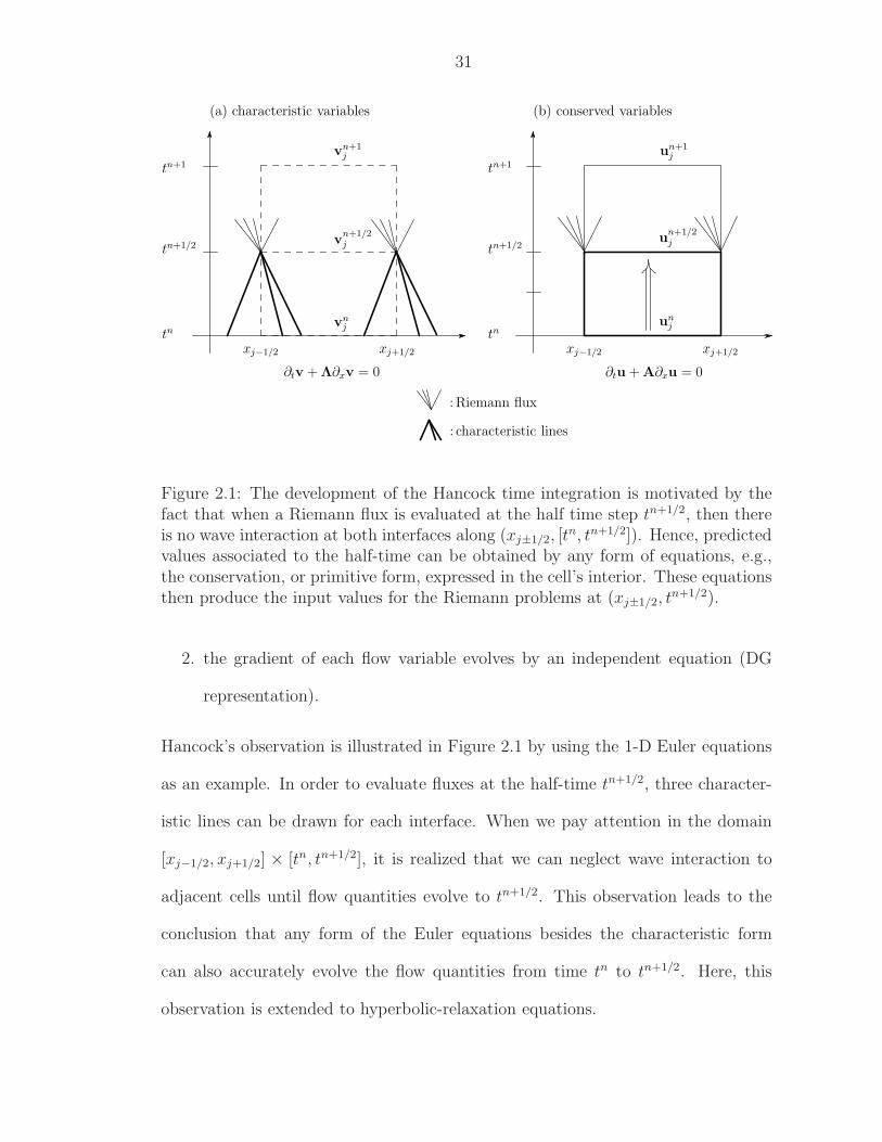
31
unj
un+1/2j
un+1j
(b) conserved variables
xj+1/2xj−1/2
tn
tn+1
tn+1/2
vn+1j
vnj
vn+1/2j
xj−1/2 xj+1/2
tn
tn+1
tn+1/2
: Riemann flux
(a) characteristic variables
∂tv + Λ∂xv = 0 ∂tu + A∂xu = 0
: characteristic lines
Figure 2.1: The development of the Hancock time integration is motivated by thefact that when a Riemann flux is evaluated at the half time step tn+1/2, then thereis no wave interaction at both interfaces along (xj±1/2, [t
n, tn+1/2]). Hence, predictedvalues associated to the half-time can be obtained by any form of equations, e.g.,the conservation, or primitive form, expressed in the cell’s interior. These equationsthen produce the input values for the Riemann problems at (xj±1/2, t
n+1/2).
2. the gradient of each flow variable evolves by an independent equation (DG
representation).
Hancock’s observation is illustrated in Figure 2.1 by using the 1-D Euler equations
as an example. In order to evaluate fluxes at the half-time tn+1/2, three character-
istic lines can be drawn for each interface. When we pay attention in the domain
[xj−1/2, xj+1/2] × [tn, tn+1/2], it is realized that we can neglect wave interaction to
adjacent cells until flow quantities evolve to tn+1/2. This observation leads to the
conclusion that any form of the Euler equations besides the characteristic form
can also accurately evolve the flow quantities from time tn to tn+1/2. Here, this
observation is extended to hyperbolic-relaxation equations.
32
As to the DG discretization, the number of discretized update equations is
twice that for the original PDEs. We denote the upwind moment scheme by
“DG(1)–Hancock method”; it looks promising in comparison to the popular method-
of-lines (MOL) approaches such as FV/DG–MOL. The MOL decouples the dis-
cretizations in space and time: first a semi-discrete form in space is evaluated, then
integrated over time by a suitable ODE solver, e.g., RKs. The upwind moment
scheme(DG(1)–Hancock
)is a fully discrete, one-step method with one intermedi-
ate update step needed for computing the volume integral of the flux. It requires
solving a Riemann problem twice at each cell interface. Based on a Fourier analysis,
the method achieves third-order accuracy in space and time. By design, the up-
wind moment scheme for a linear advection equation reduces to Van Leer’s ‘scheme
III’ [vL77], which is a DG spatial discretization with an exact shift operator for the
time evolution. It was shown that the method is linearly stable up to Courant num-
ber 1 with an upwind flux. Conversely, DG spatial discretizations combined with
MOL typically have a more strict stability condition: for DG(1)–RK2 (second-order)
the limit is1
3, and for the DG(2)–RK3 (third-order) it is
1
5[CS01, p. 190].
When discretizing hyperbolic-relaxation equations (2.1), the source term has to
be treated implicitly to ensure the stability in the stiff regime (ǫ ≪ 1). In contrast,
the advection term is treated explicitly due to the complexity of the flux evaluation.
These methods are ‘semi-implicit.’ It is expected that the stability of a method
is solely constrained by the explicit discretization, that is, by an advective CFL
condition: ∆t ∝ ∆x. This can indeed be realized; however, the simple implicit
treatment of source terms, e.g., the backward Euler method (1st-order), does not
always guarantee high-order accuracy in the stiff regime, where the source-term
effect is important.
33
The unique feature of the upwind moment scheme is the evaluation of the
space-time volume integral in the update equation of the solution gradient. Indeed,
this volume integral of the flux makes the method third-order accurate. When ap-
plying the upwind moment scheme to hyperbolic-relaxation equations, a difficulty
arises in computing the volume integral of the source term in the update equation
of the cell-average. Since the vector of cell-average variables at the next time level,
un+1, is still unknown, no simple quadrature rule in time can be used. Thus, instead
of computing the volume integral by a quadrature, we use an idea from stiff ODE
solvers to solve stiff source terms accurately. In our method, the time integral of
the source term is discretized by the two-point Gauss–Radau quadrature, which can
be regarded as an L-stable ODE solver if advection terms are omitted. The same
quadrature points are used for the volume integral of the flux in the gradient-update
equation, whereas Huynh’s original upwind moment method for conservation laws
adopts the three-point Gauss–Lobatto quadrature.
Because the source term does not contain spatial derivatives, the method is
point-implicit, that is, the implicitness is local, requiring no information from neigh-
boring cells. Previously a method for the case of a linear flux and source was pre-
sented [SvL06]; here we extend the method to a nonlinear flux and source. The
extension to multiple dimensions is also described.
2.2 DG(1)–Hancock Method for One-Dimensional Equations
2.2.1 DG Formulation
For brevity, we only consider a one-dimensional case with a uniform grid in
this section; the multidimensional extension is presented in the next section. Let
∆x := xj+1/2 − xj−1/2 be the cell width and Ij := [xj−1/2, xj+1/2] be the domain
34
of cell j. The general DG method is obtained by converting a differential equation
to a weak formulation (weighted-residual method). Here, since a DG discretization
is adopted only in space, a test function v(x) : R → R is just a function of space.
The Hancock method is adopted for time discretization. Multiplying (2.1) by a test
function, v(x), and integrating over the interval Ij leads to the semi-discrete form
of the weak formulation:
∂
∂t
∫
Ij
u(x, t)v(x) dx = −∫
Ij
∂xf(u(x, t))v(x) dx +
∫
Ij
1
ǫs(u(x, t))v(x) dx. (2.3)
Applying integration by parts on the flux term transfers the spatial differential
operator acting on the flux f(u) to the test function v(x),
∂
∂t
∫
Ij
u(x, t)v(x) dx = −f(u(x, t))v(x)
∣∣∣∣xj+1/2
xj−1/2
+
∫
Ij
f(u(x, t))∂xv(x) dx +
∫
Ij
1
ǫs(u(x, t))v(x) dx. (2.4)
To derive the fully discrete method, we integrate again in time over T n := [tn, tn+1],
∫
Ij
u(x, t)v(x) dx
∣∣∣∣tn+1
tn
︸ ︷︷ ︸Time evolution
= −∫
T n
f(u(x, t))v(x)
∣∣∣∣xj+1/2
xj−1/2
dt
︸ ︷︷ ︸Boundary integral
+
∫∫
Ij×T n
f(u(x, t))∂xv(x) dxdt
︸ ︷︷ ︸Volume integral
+
∫∫
Ij×T n
1
ǫs(u(x, t))v(x) dxdt
︸ ︷︷ ︸Volume integral
. (2.5)
Note that (2.5) is still exact in the weak formulation. To discretize the weak formula-
tion, we now approximate the exact solution u(x, t) by piecewise linear polynomials,
uh(x, t)|Ij∈ P 1, and the test function v(x) by vh(x)|Ij
∈ P 1, where the subscript
h represents the approximate solution in polynomial space. Figure 2.2 shows the
solution distribution of DG-P 1 method (a), compared to the first- (solid line) and
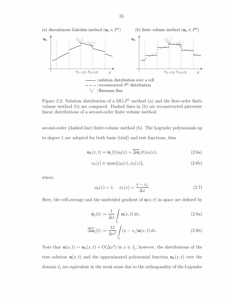
35
x
uh
xj+1/2xj−1/2
(b) finite volume method (uh ∈ P 0)
uh
x
(a) discontinous Galerkin method (uh ∈ P 1)
: solution distribution over a cell: reconstructed P 1 distribution
:Riemann flux
xj−1/2 xj+1/2
Figure 2.2: Solution distribution of a DG-P 1 method (a) and the first-order finitevolume method (b) are compared. Dashed lines in (b) are reconstructed piecewiselinear distributions of a second-order finite volume method.
second-order (dashed line) finite-volume method (b). The Legendre polynomials up
to degree 1 are adopted for both basis (trial) and test functions, thus
uh(x, t) = uj(t)φ0(x) + ∆uj(t)φ1(x), (2.6a)
vh(x) ∈ spanφ0(x), φ1(x), (2.6b)
where
φ0(x) = 1, φ1(x) =x − xj
∆x. (2.7)
Here, the cell-average and the undivided gradient of u(x, t) in space are defined by
uj(t) :=1
∆x
∫
Ij
u(x, t) dx, (2.8a)
∆uj(t) :=12
∆x2
∫
Ij
(x − xj)u(x, t) dx. (2.8b)
Note that u(x, t) = uh(x, t) + O(∆x2) in x ∈ Ij ; however, the distributions of the
true solution u(x, t) and the approximated polynomial function uh(x, t) over the
domain Ij are equivalent in the weak sense due to the orthogonality of the Legendre
36
polynomials,
∫
Ij
u(x, t)φk(x) dx ≡∫
Ij
uh(x, t)φk(x) dx, k = 0, 1. (2.9)
Once the basis and test functions are chosen, approximate governing equations are
derived by adopting the basis functions φ0(x) and φ1(x) as the test function vh(x).
Inserting φi(x) into vh(x) leads to two independent update equations:
• v(x) = 1 :
∫
Ij
uh(x, t) dx
∣∣∣∣tn+1
tn= −
∫
T n
f(uh(x, t))
∣∣∣∣xj+1/2
xj−1/2
dt +
∫∫
Ij×T n
1
ǫs(uh(x, t)) dxdt, (2.10a)
• v(x) =x − xj
∆x:
∫
Ij
uh(x, t)x − xj
∆xdx
∣∣∣∣tn+1
tn= −
∫
T n
f(uh(x, t))x − xj
∆x
∣∣∣∣xj+1/2
xj−1/2
dt
+1
∆x
∫∫
Ij×T n
f(uh(x, t)) dxdt +
∫∫
Ij×T n
1
ǫs(uh(x, t))
x − xj
∆xdxdt. (2.10b)
The time-evolution term and boundary integral can be further simplified by insert-
ing (2.6a) into uh(x, t), then
∆x[un+1
j − unj
]= −
∫
T n
[fj+1/2(t) − fj−1/2(t)
]dt
︸ ︷︷ ︸Boundary integral
+
∫∫
Ij×T n
1
ǫs(uh(x, t)) dxdt
︸ ︷︷ ︸Volume integral
, (2.11a)
∆x
12
[∆u
n+1
j − ∆un
j
]= −1
2
∫
T n
[fj+1/2(t) + fj−1/2(t)
]dt
︸ ︷︷ ︸Boundary integral
+1
∆x
∫∫
Ij×T n
f(uh(x, t)) dxdt
︸ ︷︷ ︸Volume integral
+
∫∫
Ij×T n
1
ǫs(uh(x, t))
x − xj
∆xdxdt
︸ ︷︷ ︸Volume integral
, (2.11b)
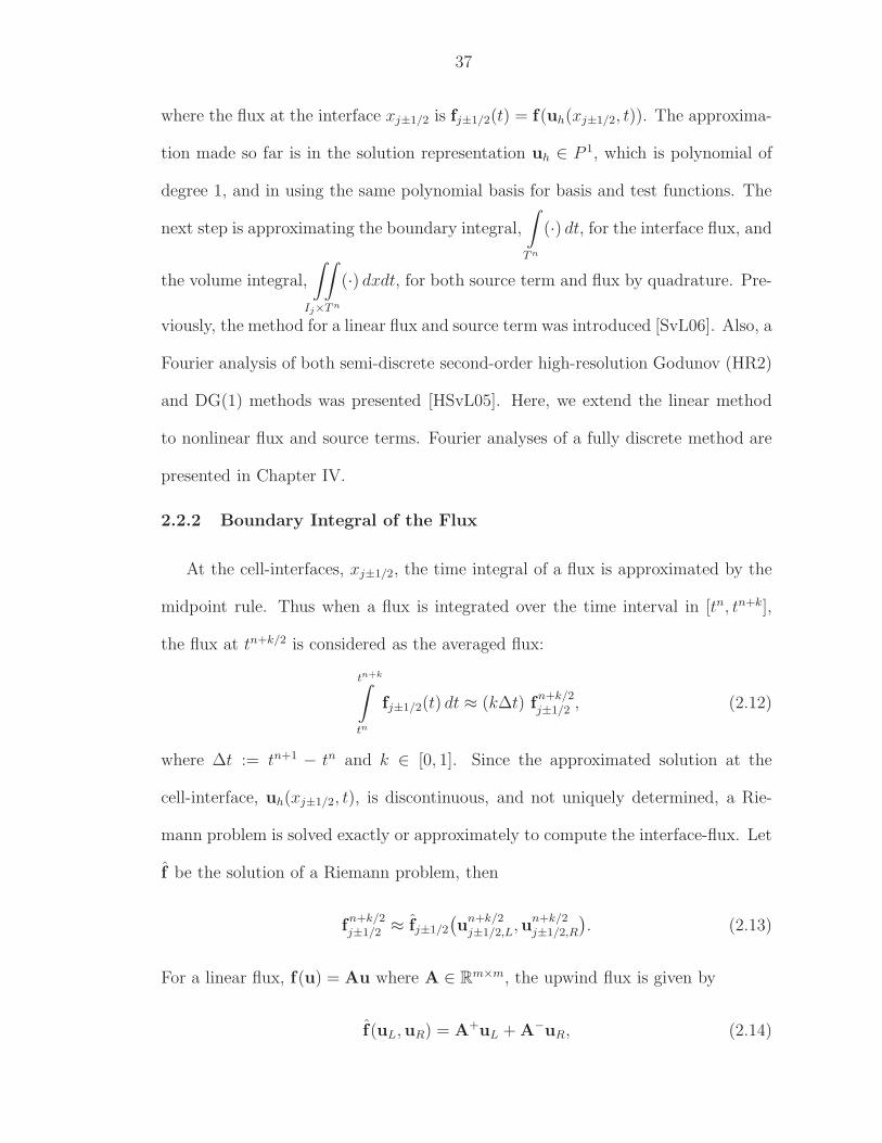
37
where the flux at the interface xj±1/2 is fj±1/2(t) = f(uh(xj±1/2, t)). The approxima-
tion made so far is in the solution representation uh ∈ P 1, which is polynomial of
degree 1, and in using the same polynomial basis for basis and test functions. The
next step is approximating the boundary integral,
∫
T n
(·) dt, for the interface flux, and
the volume integral,
∫∫
Ij×T n
(·) dxdt, for both source term and flux by quadrature. Pre-
viously, the method for a linear flux and source term was introduced [SvL06]. Also, a
Fourier analysis of both semi-discrete second-order high-resolution Godunov (HR2)
and DG(1) methods was presented [HSvL05]. Here, we extend the linear method
to nonlinear flux and source terms. Fourier analyses of a fully discrete method are
presented in Chapter IV.
2.2.2 Boundary Integral of the Flux
At the cell-interfaces, xj±1/2, the time integral of a flux is approximated by the
midpoint rule. Thus when a flux is integrated over the time interval in [tn, tn+k],
the flux at tn+k/2 is considered as the averaged flux:
tn+k∫
tn
fj±1/2(t) dt ≈ (k∆t) fn+k/2j±1/2 , (2.12)
where ∆t := tn+1 − tn and k ∈ [0, 1]. Since the approximated solution at the
cell-interface, uh(xj±1/2, t), is discontinuous, and not uniquely determined, a Rie-
mann problem is solved exactly or approximately to compute the interface-flux. Let
f be the solution of a Riemann problem, then
fn+k/2j±1/2 ≈ fj±1/2
(u
n+k/2j±1/2,L,u
n+k/2j±1/2,R
). (2.13)
For a linear flux, f(u) = Au where A ∈ Rm×m, the upwind flux is given by
f(uL,uR) = A+uL + A−uR, (2.14)
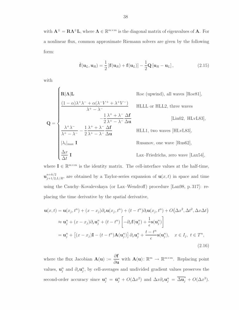
38
with A± = RΛ±L, where Λ ∈ Rm×m is the diagonal matrix of eigenvalues of A. For
a nonlinear flux, common approximate Riemann solvers are given by the following
form:
f(uL,uR) =1
2[f(uR) + f(uL)] − 1
2Q [uR − uL] , (2.15)
with
Q =
R|Λ|L Roe (upwind), all waves [Roe81],
(1 − α)λ+λ− + α(λ−V + + λ+V −)
λ+ − λ−HLLL or HLL2, three waves
−1
2
λ+ + λ−
λ+ − λ−
∆f
∆u[Lin02, HLvL83],
λ+λ−
λ+ − λ−− 1
2
λ+ + λ−
λ+ − λ−
∆f
∆uHLL1, two waves [HLvL83],
|λi|max I Rusanov, one wave [Rus62],
∆x
∆tI Lax–Friedrichs, zero wave [Lax54],
where I ∈ Rm×m is the identity matrix. The cell-interface values at the half-time,
un+k/2j+1/2,L/R, are obtained by a Taylor-series expansion of u(x, t) in space and time
using the Cauchy–Kovalevskaya (or Lax–Wendroff) procedure [Lan98, p. 317]: re-
placing the time derivative by the spatial derivative,
u(x, t) = u(xj , tn) + (x − xj)∂xu(xj , t
n) + (t − tn)∂tu(xj , tn) + O
(∆x2, ∆t2, ∆x∆t
)
≈ unj + (x − xj)∂xu
nj + (t − tn)
[−∂xf(u
nj ) +
1
ǫs(un
j )
]
= unj +
[(x − xj)I − (t − tn)A(un
j )]∂xu
nj +
t − tn
ǫs(un
j ), x ∈ Ij, t ∈ T n,
(2.16)
where the flux Jacobian A(u) :=∂f
∂uwith A(u) : Rm → Rm×m. Replacing point
values, unj and ∂xu
nj , by cell-averages and undivided gradient values preserves the
second-order accuracy since unj = un
j + O(∆x2) and ∆x∂xunj = ∆u
n
j + O(∆x3).
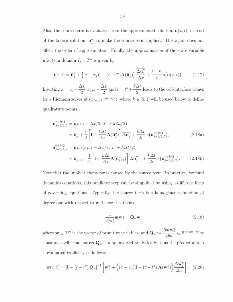
39
Also, the source term is evaluated from the approximated solution, u(x, t), instead
of the known solution, unj , to make the source term implicit. This again does not
affect the order of approximation. Finally, the approximation of the state variable
u(x, t) in domain Ij × T n is given by
u(x, t) ≈ unj +
[(x − xj)I− (t − tn)A(un
j )] ∆u
n
j
∆x+
t − tn
ǫs(u(x, t)
). (2.17)
Inserting x = xj +∆x
2, xj+1−
∆x
2and t = tn +
k∆t
2leads to the cell-interface values
for a Riemann solver at (xj+1/2, tn+k/2), where k ∈ [0, 1] will be used below to define
quadrature points:
un+k/2j+1/2,L = uj(xj + ∆x/2, tn + k∆t/2)
= unj +
1
2
[I − k∆t
∆xA(un
j )
]∆u
n
j +k∆t
2ǫs(u
n+k/2j+1/2,L
), (2.18a)
un+k/2j+1/2,R = uj+1(xj+1 − ∆x/2, tn + k∆t/2)
= unj+1 −
1
2
[I +
k∆t
∆xA(un
j+1)
]∆u
n
j+1 +k∆t
2ǫs(u
n+k/2j+1/2,R
). (2.18b)
Note that the implicit character is caused by the source term. In practice, for fluid
dynamics equations, this predictor step can be simplified by using a different form
of governing equations. Typically, the source term is a homogeneous function of
degree one with respect to w, hence it satisfies
1
ǫ(w)s(w) = Qww, (2.19)
where w ∈ Rm is the vector of primitive variables, and Qw :=∂s(w)
∂w∈ Rm×m. The
constant coefficient matrix Qw can be inverted analytically, thus the predictor step
is evaluated explicitly as follows:
w(x, t) = [I − (t − tn)Qw]−1
[wn
j +((x − xj) I− (t − tn)A(wn
j ))∆wn
j
∆x
]. (2.20)
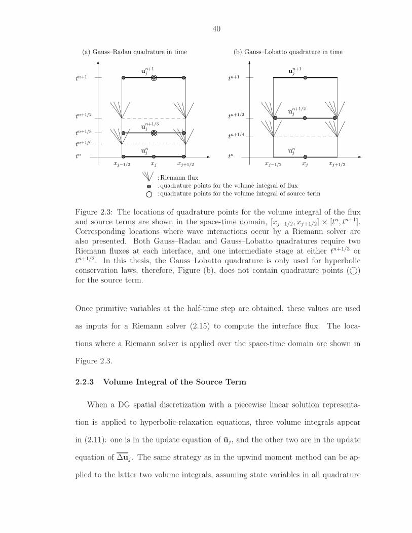
40
unj
un+1/2j
un+1j
(b) Gauss–Lobatto quadrature in time
xj+1/2xj−1/2
tn+1/4
xj
tn
tn+1
tn+1/2
un+1j
un+1/3j
unj
xj−1/2 xj+1/2
tn+1/3
tn+1/6
xj
tn
tn+1
tn+1/2
: quadrature points for the volume integral of flux:Riemann flux
: quadrature points for the volume integral of source term
(a) Gauss–Radau quadrature in time
Figure 2.3: The locations of quadrature points for the volume integral of the fluxand source terms are shown in the space-time domain, [xj−1/2, xj+1/2] × [tn, tn+1].Corresponding locations where wave interactions occur by a Riemann solver arealso presented. Both Gauss–Radau and Gauss–Lobatto quadratures require twoRiemann fluxes at each interface, and one intermediate stage at either tn+1/3 ortn+1/2. In this thesis, the Gauss–Lobatto quadrature is only used for hyperbolicconservation laws, therefore, Figure (b), does not contain quadrature points (©)for the source term.
Once primitive variables at the half-time step are obtained, these values are used
as inputs for a Riemann solver (2.15) to compute the interface flux. The loca-
tions where a Riemann solver is applied over the space-time domain are shown in
Figure 2.3.
2.2.3 Volume Integral of the Source Term
When a DG spatial discretization with a piecewise linear solution representa-
tion is applied to hyperbolic-relaxation equations, three volume integrals appear
in (2.11): one is in the update equation of uj , and the other two are in the update
equation of ∆uj. The same strategy as in the upwind moment method can be ap-
plied to the latter two volume integrals, assuming state variables in all quadrature
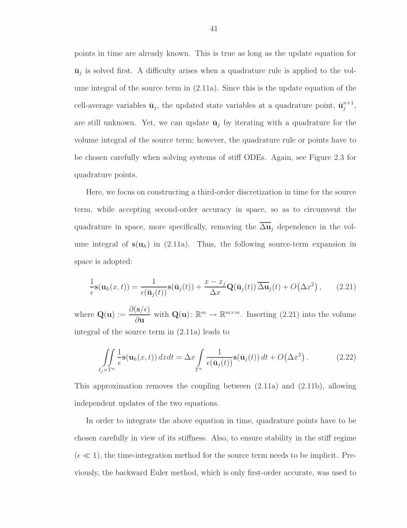
41
points in time are already known. This is true as long as the update equation for
uj is solved first. A difficulty arises when a quadrature rule is applied to the vol-
ume integral of the source term in (2.11a). Since this is the update equation of the
cell-average variables uj , the updated state variables at a quadrature point, un+1j ,
are still unknown. Yet, we can update uj by iterating with a quadrature for the
volume integral of the source term; however, the quadrature rule or points have to
be chosen carefully when solving systems of stiff ODEs. Again, see Figure 2.3 for
quadrature points.
Here, we focus on constructing a third-order discretization in time for the source
term, while accepting second-order accuracy in space, so as to circumvent the
quadrature in space, more specifically, removing the ∆uj dependence in the vol-
ume integral of s(uh) in (2.11a). Thus, the following source-term expansion in
space is adopted:
1
ǫs(uh(x, t)) =
1
ǫ(uj(t))s(uj(t)) +
x − xj
∆xQ(uj(t)) ∆uj(t) + O
(∆x2
), (2.21)
where Q(u) :=∂(s/ǫ)
∂uwith Q(u) : Rm → Rm×m. Inserting (2.21) into the volume
integral of the source term in (2.11a) leads to
∫∫
Ij×T n
1
ǫs(uh(x, t)) dxdt = ∆x
∫
T n
1
ǫ(uj(t))s(uj(t)) dt + O
(∆x3
). (2.22)
This approximation removes the coupling between (2.11a) and (2.11b), allowing
independent updates of the two equations.
In order to integrate the above equation in time, quadrature points have to be
chosen carefully in view of its stiffness. Also, to ensure stability in the stiff regime
(ǫ ≪ 1), the time-integration method for the source term needs to be implicit. Pre-
viously, the backward Euler method, which is only first-order accurate, was used to
42
s-stage RK method order p stage order p linear stability nonlinear stability
Gauss 2s s A-stability algebraic stability
Radau IA 2s− 1 s− 1 L-stability algebraic stabilityRadau IIA 2s− 1 s L-stability algebraic stability
Lobatto IIIA 2s− 2 s A-stability No algebraic stabilityLobatto IIIB 2s− 2 s− 2 A-stability No algebraic stabilityLobatto IIIC 2s− 2 s− 1 L-stability algebraic stability
Table 2.1: The properties of the classes of implicit Runge–Kutta methods are tab-ulated [Lam91]. The order p is based on the linear theory, and the stage order p isthe lower bound obtained by the nonlinear theory. Thus, in general, the order of amethod is within [p, p].
integrate the source term and obtain the intermediate stage [SvL06]. Unfortunately,
linear analysis shows that the source-term discretization is overall only second-order
accurate due to the first-order temporal discretization in the intermediate step. In
order to achieve high-order accuracy and circumvent the stiffness, a fully-implicit
method is preferable. The properties of the classes of implicit Runge–Kutta meth-
ods are tabulated in Table 2.1 [Lam91, p. 250, 282]. Based on these properties, the
Radau IA, Radau IIA, and Lobatto IIIC methods, which possess both L-stability
and nonlinear stability, are candidates for time integration of the source term. In
order to achieve third-order accuracy in time, the Radau IA/IIA methods require
only two stages (s = 2, p = 3), whereas the Lobatto IIIC method requires three
stages (s = 3, p = 4). To minimize the computational cost of the fully-implicit
procedure for the source term in a scheme, we chose the former, particularly the
Radau IIA method, for the source-term integral. (This is an original contribution.)
Hence, the volume integral of the source term is approximated as
∫∫
Ij×T n
1
ǫs(uh(x, t)) dxdt ≈ ∆x∆t
[3
4
s(un+1/3j )
ǫ(un+1/3j )
+1
4
s(un+1j )
ǫ(un+1j )
], (2.23)
43
where a new intermediate stage at time level n +1
3is introduced. Figure 2.3(a)
shows the quadrature points of the Radau IIA method for the source term by the
circle symbol (©). The overall update equations are given by
un+1/3j = un
j − ∆t
3
1
∆x
[fn+1/6j+1/2 − f
n+1/6j−1/2
]
︸ ︷︷ ︸explicit
+∆t
3
[5
4
s(un+1/3j )
ǫ(un+1/3j )
− 1
4
s(un+1j )
ǫ(un+1j )
]
︸ ︷︷ ︸implicit
, (2.24a)
un+1j = un
j − ∆t
∆x
[fn+1/2j+1/2 − f
n+1/2j−1/2
]
︸ ︷︷ ︸explicit
+∆t
[3
4
s(un+1/3j )
ǫ(un+1/3j )
+1
4
s(un+1j )
ǫ(un+1j )
]
︸ ︷︷ ︸implicit
. (2.24b)
To solve this system numerically, first the interface fluxes are computed explicitly.
Then, the problem reduces to finding the solutions of systems of nonlinear algebraic
equations of the following form:
uA = Cf + Cs sA(uA), (2.25)
where
uA =
un+1/3j
un+1j
, sA(uA) =
s(un+1/3j )
ǫ(un+1/3j )
s(un+1j )
ǫ(un+1j )
, (2.26a)
Cf =
unj − ∆t
3
1
∆x
[fn+1/6j+1/2 − f
n+1/6j−1/2
]
unj − ∆t
∆x
[fn+1/2j+1/2 − f
n+1/2j−1/2
]
, Cs = ∆t
5
12I − 1
12I
3
4I
1
4I
, (2.26b)
with uA,Cf ∈ R2m,Cs ∈ R
2m×2m, and sA(uA) : R2m → R
2m. Here, the New-
ton–Raphson method is employed to find the solution, thus the iteration process at
step p is given by
up+1A = up
A − [IA − CsQA(upA)]
−1[up
A −Cf − Cs sA(upA)] , p = 0, 1, 2 . . . , (2.27)
where
QA(uA) :=∂sA
∂uA=
Q(un+1/3j ) 0
0 Q(un+1j )
, QA(uA) : R
2m → R2m×2m, (2.28)
44
and IA ∈ R2m×2m. To start up the iteration, the initial guess at the time level n,
u0A =
[un
j ; unj
], is used. The iteration on the system of 2m equations can be reduced
to 2(m − l) equations where l < n, since the first l entries of the source term are
zero.
In general, when the Newton–Raphson method is implemented, it is more ef-
ficient to adopt LU -decomposition to the matrix [IA −CsQA(upA)], and solve the
system of linear algebraic equations instead of inverting it. However, the structure
of the source term is typically simple, and the inverse matrix, [IA − CsQA(upA)]−1,
can be obtained analytically as a function of uA. The advantage of the choice
of hyperbolic-relaxation equations over the NS equations is clear here: since the
method is point-implicit due to the source term, the inverse of the matrix is still lo-
cal, whereas the implicit treatment of the diffusion term in the NS equations makes
the domain of dependence global.
2.2.4 Volume Integral of the Flux
Gauss–Lobatto Points (Original Upwind Moment Scheme)
First, we review Huynh’s original upwind moment scheme [Huy06a]. The method
utilizes the three-point Gauss–Lobatto quadrature (see Figure 2.3(b)) for both space
and time integration of the flux, thus the volume integral of the flux is approximated
by
∫∫
Ij×T n
f(uh(x, t)) dxdt ≈ ∆t
∫
Ij
1
6
[f(u(x, tn)) + 4f(u(x, tn+1/2)) + f(u(x, tn+1))
]dx
≈ ∆t
∫
Ij
f(u(x)) dx
≈ ∆t∆x
6
[f(u(xj−1/2)) + 4f(u(xj)) + f(u(xj+1/2))
], (2.29)
45
where
u(x) = ˆuj + ∆ujx − xj
∆x, (2.30a)
ˆuj =1
6
(un
j + 4un+1/2j + un+1
j
), (2.30b)
∆uj =1
2
(∆u
n
j + ∆un+1
j
). (2.30c)
Here, (·) denotes a time-averaged value. When the discretization of conservation
laws, (2.11) with s = 0, is considered, the volume integral appears only in the second
equation (2.11b). Since the cell-average variables are updated in the first equation,
un+1j is already known when the volume integral in the second equation is evaluated.
Thus ˆuj is evaluated explicitly whereas ∆un+1
j in (2.30c) is still unknown, and an
iterative process is required. To start the iteration, the slope at the time level n
is used as the initial guess; however, Huynh reported that no improvement was
observed by iterations, and suggested to replace (2.30c) by
∆uj = ∆un
j . (2.31)
When the flux is linear, f(u) = Au, the volume integral (2.29) is evaluated exactly
in space and approximately in time, thus
∫∫
Ij×T n
f(uh(x, t)) dxdt = ∆xA
∫
T n
uj(t) dt
≈ ∆x∆t Aˆuj , (2.32)
where ˆuj is given by (2.30b). In (2.30b), the new intermediate stage, un+1/2j , is
introduced, and computed in advance by updating over a half time step:
un+1/2j = un
j − 1
∆x
tn+1/2∫
tn
[fj+1/2(t) − fj−1/2(t)
]dt
= unj − ∆t
2
1
∆x
[fn+1/4j+1/2 − f
n+1/4j−1/2
]. (2.33)
46
Note that the method only requires the cell-average value at the half-time step,
not the undivided gradient, since the slope at the time level n is used in the entire
space-time domain according to (2.31). Once the intermediate state is obtained,
from (2.11), the final update equations become
un+1j = un
j − ∆t
∆x
[fn+1/2j+1/2 − f
n+1/2j−1/2
], (2.34a)
∆un+1
j = ∆un
j − ∆t
∆x6
[fn+1/2j+1/2 + f
n+1/2j−1/2 − 2
∆x∆tf(uj)
], (2.34b)
where f(uj) is given by (2.29). In summary, the original upwind moment scheme
is a one-step method with one intermediate stage for the volume integral, requiring
two Riemann solvers at each cell-interface.
Gauss–Radau Points
When the hyperbolic-relaxation equations are considered, quadrature points for
the flux in (2.11b) need to be modified based on the quadrature for the source term.
Since we adopt the two-point Radau IIA method (2.23) as the time integrator for
the source term, the same Radau points are employed for the volume integral of
the flux. The bullet symbols (•) in Figure 2.3(a) on page 40 represent the location
of quadrature points for the flux over the space-time domain. Consequently, the
Gauss–Radau quadrature in time and the Gauss–Lobatto quadrature in space are
applied:
∫∫
Ij×T n
f(uh(x, t)
)dxdt = ∆t
∫
Ij
[3
4f(u(x, tn+1/3)
)+
1
4f(u(x, tn+1)
)]dx + O
(∆t4)
≈ ∆x∆t
(3
4fn+1/3 +
1
4fn+1
), (2.35)
47
where
fk =1
6
[f(uk
j−1/2
)+ 4f
(uk
j
)+ f(uk
j+1/2
)], (2.36a)
uk(x) = ukj + ∆u
n
j
x − xj
∆x. (2.36b)
Here, the undivided gradient is frozen at the time level n in order to keep the treat-
ment explicit. In the update equation of the undivided gradient, the intermediate-
stage value, ∆un+1/3
j , is required, and another volume integral of the flux over the
time domain T n′
= [tn, tn+1/3] is needed. Unlike in the method for hyperbolic
conservation laws, the intermediate slope quantities are necessary due to the fully
implicit treatment of the source term. Since the flux is not a stiff term and the cell-
averaged variables at the quadrature points k = 0,1
3are known, the trapezoidal
rule is applied in time while the Gauss–Lobatto quadrature is applied in space:
∫∫
Ij×T n′
f(uh(x, t)
)dxdt =
∆t
3
∫
Ij
1
2
[f(u(x, tn)
)+ f(u(x, tn+1/3)
)]dx + O
(∆t3)
≈ ∆x∆t
6
(fn + fn+1/3
), (2.37)
where spatial averaged fluxes are obtained by (2.36).
2.2.5 Integral of the Moment of the Source Term
The second-order approximation of the source term, (2.21), is inserted into the
volume integral of the moment of the source term in (2.11b), and the Gauss–Radau
quadrature is used in time:
∫∫
Ij×T n
1
ǫs(uh(x, t))
x − xj
∆xdxdt =
∆x
12
∫
T n
Q(uj(t))∆uj(t) dt + O(∆x3
)
≈ ∆x∆t
12
[3
4Q(u
n+1/3j )∆u
n+1/3
j +1
4Q(un+1
j )∆un+1
j
].
(2.38)
48
Following the same procedure as the cell-average update, the Radau IIA method
is adopted for the source term, and the final update formulas for the undivided
gradient are given by
∆un+1/3
j = ∆un
j − ∆t
3
6
∆x
[fn+1/6j+1/2 + f
n+1/6j−1/2 − 2
∆x∆tf(u
n+1/6j )
]
︸ ︷︷ ︸explicit
+∆t
3
1
ǫ
[5
4Q(u
n+1/3j )∆u
n+1/3
j − 1
4Q(un+1
j )∆un+1
j
]
︸ ︷︷ ︸implicit
,
(2.39a)
∆un+1
j = ∆un
j − ∆t
∆x6
[fn+1/2j+1/2 + f
n+1/2j−1/2 − 2
∆x∆tf(u
n+1/2j )
]
︸ ︷︷ ︸explicit
+∆t
ǫ
[3
4Q(u
n+1/3j )∆u
n+1/3
j +1
4Q(un+1
j )∆un+1
j
]
︸ ︷︷ ︸implicit
,
(2.39b)
where f(un+1/6j ) and f(u
n+1/2j ) are obtained by (2.37) and (2.35) respectively. Once
the interface fluxes and volume integrals of fluxes are computed explicitly, the prob-
lem is reduced to solving a system of linear algebraic equations:
∆uA = ∆Cf + CsQA(uA)∆uA, (2.40)
where
∆uA =
∆un+1/3
j
∆un+1
j
, (2.41a)
∆Cf =
∆un
j − ∆t
3
6
∆x
[fn+1/6j+1/2 + f
n+1/6j−1/2 − 2
∆x∆tf(u
n+1/6j )
]
∆un
j − ∆t
∆x6
[fn+1/2j+1/2 + f
n+1/2j−1/2 − 2
∆x∆tf(u
n+1/2j )
]
, (2.41b)
with ∆uA, ∆Cf ∈ R2m. Since uA is already known by (2.27), no iteration is required,
and ∆uA is obtained by
∆uA = [IA − CsQA(uA)]−1 ∆Cf. (2.42)
49
As mentioned previously, the structure of the source term is typically simple; the
inverse of the above matrix can be obtained analytically.
2.3 Extension to Multidimensional Equations
In this section, we extend the 1-D DG(1)–Hancock method described in the
previous section to multidimensional problems. Here, we closely follow the notations
conventionally adopted in the finite-element community. Nevertheless, sufficient
explanations of notations and terminologies are provided for those who are more
accustomed to finite-volume or finite-difference methodologies. Interested readers
are referred to the following books for the rigorous mathematical foundation of the
finite-element methodology: [ZTZ05, FFS03, BS02].
As to the semi-discrete discontinuous Galerkin methods combined with Runge–
Kutta time-marching (DG(k)–RK methods), Cockburn and Shu extended their
one-dimensional formulation [CLS89] to triangular grids [CHS90]; later, Bey and
Oden extended such methods to quadrilateral elements of arbitrary polynomial de-
gree [BO91]. Prior to the development of multidimensional DG(k)–RK methods,
Allmaras and Giles indeed developed the semi-discrete P 1 discontinuous Galerkin
method combined with the third-order Runge–Kutta method, DG(1)–RK3, for
quadrilateral elements [AG87, All89]. However, they did not denote their method
as a discontinuous Galerkin method, and this might be a reason why their seminal
work is little known in the community nowadays. Their method is the direct exten-
sion of Van Leer’s scheme III (for a scalar linear equation) to the two-dimensional
Euler/NS equations.
Subsequently, Halt and Agarwal extended the Allmaras–Giles method to higher
order and triangular elements, and they denote the method as the “moment method”
50
[HA92, AH99]. Borrel and Berde also adopted the moment approach, and pre-
sented a few numerical results for the two-dimensional Euler and Navier–Stokes
equations [BB95, BB98]. The specific aspect of the moment method is that, even
though the formulation is now recognized as a semi-discrete discontinuous Galerkin
method, the method is discretized directly on the physical domain except for the
volume integral; a typical DG method is discretized in a local (ξ, η) coordinate sys-
tem, to which the original governing equations, expressed in (x, y), are transformed.
An advantage of the formulation of the moment method is that the update equation
for the cell-averaged quantities is always independent of the other update equations
for slopes. In this section, the spatial approach of the moment method is taken, yet
time integration is done by the Hancock method.
2.3.1 Ritz–Galerkin Method
The system of multidimensional hyperbolic-relaxation equations is given by
∂tu(x, t) + ∇ · f(u(x, t)) =1
ǫs(u(x, t)); x ∈ Ω, t > 0, (2.43)
where u ∈ Rm is the vector of conserved quantities, f ∈ Rm×3 is the 3-D flux tensor,
s ∈ Rm is the source vector for the conservation form, and Ω is the domain of
interest. Let T be a time interval, then the solution u(x, t) in (2.43) is defined over
the entire spatial domain Ω and temporal domain, i.e. u(x, t) ∈ Ω×T . Figure 2.4(a)
shows a schematic of notations introduced in the above equation. By specifying
the initial condition, u(x, 0) = u0(x), and sufficient boundary conditions along
boundary ∂Ω, the problem statement of the differential equations (2.43) is:
Find u(x, t) such that the solution u(x, t) satisfies (2.43) for any x ∈ Ω
and any t ∈ T .
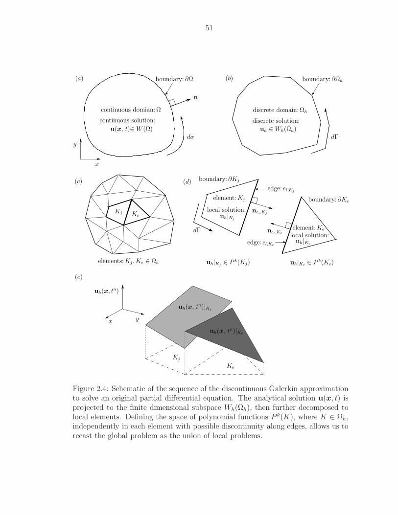
51
x
uh(x, tn)
y
continuous domian:Ω
boundary: ∂Ω
discrete domain:Ωh
boundary: ∂Ωh
Kj Ke
element:Kj
element:Ke
boundary: ∂Kj
nei,Kj
edge: ei,Kj
nel,Ke
edge: el,Ke
boundary: ∂Ke
elements:Kj , Ke ∈ Ωh
local solution:
discrete solution:
uh|Kj
local solution:uh|Ke
uh|Kj∈ P k(Kj) uh|Ke ∈ P k(Ke)
x
y
(a) (b)
(c) (d)
continuous solution:
uh ∈ Wh(Ωh)u(x, t)∈ W (Ω)dσ dΓ
dΓ
n
(e)
uh(x, tn)|Ke
uh(x, tn)|Kj
Kj
Ke
Figure 2.4: Schematic of the sequence of the discontinuous Galerkin approximationto solve an original partial differential equation. The analytical solution u(x, t) isprojected to the finite dimensional subspace Wh(Ωh), then further decomposed tolocal elements. Defining the space of polynomial functions P k(K), where K ∈ Ωh,independently in each element with possible discontinuity along edges, allows us torecast the global problem as the union of local problems.
52
Since the solution u(x, t) is defined over the continuous space-time domain, it is
impossible to represent the true solution u(x, t) on a digital computer with a finite
resource of memory or storage. Thus we make an assumption that the true solution
can be accurately approximated by a finite number of functions such that
u(x, t) ≈ uh(x, t) =∑
i
ci(x, t)φi(x, t), (2.44)
where the coefficients ci(x, t) are called the degrees of freedom, and φi(x, t) the trial
(basis) functions. Our goal is to construct the evolution equations of the degrees
of freedom ci(x, t) to compute an approximate solution of the original differential
equations (2.43). In general, the procedure of projecting a solution defined in an
infinite-dimensional space W (Ω) to an approximating solution like (2.44) in a finite
dimensional space Wh(Ωh) is called the Ritz–Galerkin method. More specifically,
the Ritz–Galerkin method can be subdivided to the Ritz method, which employs a
variational formulation, and the weighted-residual method, where a weak formula-
tion is applied. See Figure 2.5 for their hierarchical relations [KS05, FFS03, DH03]
A brief summary of these methods are as follows:
• Ritz method, or also called Rayleigh–Ritz method (variational formulation):
An variational principle equivalent to the original differential equations is for-
mulated, and the original problem is recast as the minimization problem for
the variational formulation. For instance, the solution of physical problem
expressed in differential form is restated as the extremum of a function. A
drawback of this approach is that constructing a variational formulation might
not be possible for complex physical systems such as the Navier–Stokes equa-
tions.
• Weighted residual method (weak formulation):
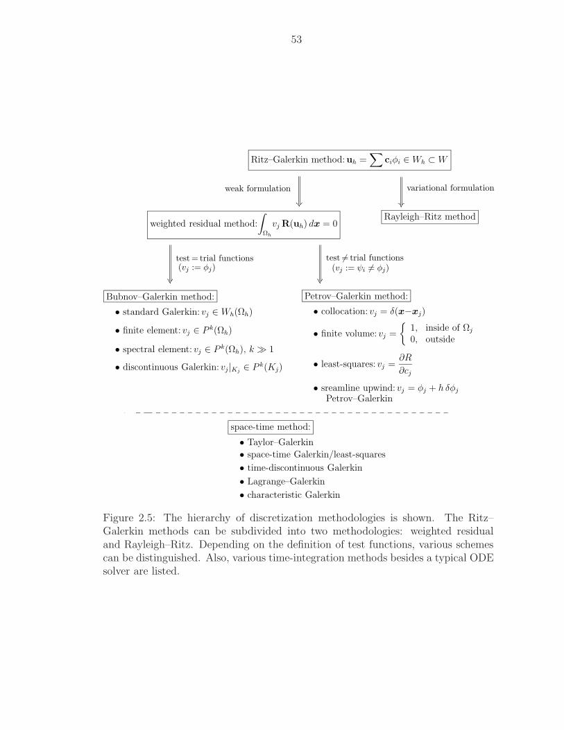
53
Ritz–Galerkin method:uh =∑
ciφi ∈ Wh ⊂ W
weighted residual method:
∫
Ωh
vj R(uh) dx = 0Rayleigh–Ritz method
variational formulationweak formulation
Bubnov–Galerkin method: Petrov–Galerkin method:
• standard Galerkin: vj ∈ Wh(Ωh)
• finite element: vj ∈ P k(Ωh)
• collocation: vj = δ(x−xj)
• finite volume: vj =
1, inside of Ωj
0, outside
• least-squares: vj =∂R
∂cj
(vj := ψi 6= φj)(vj := φj)test = trial functions test 6= trial functions
• discontinuous Galerkin: vj |Kj∈ P k(Kj)
• spectral element: vj ∈ P k(Ωh), k ≫ 1
• sreamline upwind: vj = φj + h δφj
Petrov–Galerkin
space-time method:
• Taylor–Galerkin
• space-time Galerkin/least-squares
• time-discontinuous Galerkin
• Lagrange–Galerkin
• characteristic Galerkin
Figure 2.5: The hierarchy of discretization methodologies is shown. The Ritz–Galerkin methods can be subdivided into two methodologies: weighted residualand Rayleigh–Ritz. Depending on the definition of test functions, various schemescan be distinguished. Also, various time-integration methods besides a typical ODEsolver are listed.
54
The original differential equation is rewritten in an integral form through
a weak formulation. This approach is less restrictive and can be applied
to a physical problem that does not have a variational formulation. Nev-
ertheless, if a variational formulation can be obtained for a certain problem,
both variational and weighted-residual methods lead to an identical discretiza-
tion. The Galerkin weighted-residual method can be further subdivided into
Bubnov–Galerkin, and Petrov–Galerkin methods. Bubnov–Galerkin meth-
ods, often simply called Galerkin methods, set test functions identical to trial
functions, whereas Petrov–Galerkin methods employ different functions. In
the case when an approximation of the solution in (2.44) is piecewise polyno-
mial, a Bubnov/Petrov–Galerkin method is particularly called a finite-element
method. Hence, it is more appropriate to call a DG method, for instance, a
discontinuous Bubnov–Galerkin finite-element method.
Here, we employ the method of weighted residuals, more precisely a discontinuous
Galerkin method, which is one of the Bubnov–Galerkin methods, to obtain the
discretization method. The procedure to obtain the weak formulation is explained
in the next section.
2.3.2 Weak Formulation
At first, we define a scalar function in the same space as the solution u(x, t),
and denote it as v(x, t) ∈ Ω × T . This is called the test function. Multiplying
the original differential equations (2.43) by a test function, v(x, t), and integrating
over the space-time domain Ω(t) × T leads to the weak formulation of the original
55
differential equations:
∫∫
Ω(t)×T
∂tu(x, t) v(x, t) dxdt = −∫∫
Ω(t)×T
∇ · f(u(x, t)) v(x, t) dxdt
+
∫∫
Ω(t)×T
1
ǫs(u(x, t)) v(x, t) dxdt. (2.45)
The weak formulation of the problem is:
Find u(x, t) such that the solution u(x, t) satisfies (2.45) for any test
function v(x, t) ∈ Ω × T .
Note that the problem is still defined in an infinite-dimensional space. In order
to remove derivatives of the solution and its flux from the space-time integrals, we
integrate by parts, yielding the equalities
∫
T
∂tu(x, t)v(x, t) dt ≡ [u(x, t) v(x, t)]t2t1 −∫
T
u(x, t) ∂tv(x, t)dt, (2.46a)
∫
Ω(t)
∇ · f(u) v(x) dx ≡∫
∂Ω(t)
v(x) f · n dσ −∫
Ω(t)
∇v(x) · f(u) dx; (2.46b)
these are inserted into the weak formulation (2.45). Here, n is the outward unit
vector normal to the boundary ∂Ω(t), and T := [t1, t2]. The integration variable
σ in the right hand side of (2.46b) is defined along the boundary ∂Ω(t). See also
Figure 2.4(a) illustrating their definitions.
In the course of its derivation, one might wonder why a DG method always
relies on integration by parts. The reason is that the integration by parts transfers
a differential operator acting on nonlinear functions to test functions. For instance,
the divergence operator, ∇·, applied to the nonlinear flux f(u) on the left hand side
of (2.46b) is now acting on a gradient operator, ∇, on a test function v(x) on the
right hand side. This operation is not unique to DG methods: weighted-residual
56
methods in general take advantage of it. For instance, a finite volume method uses
the same technique in its derivation. This can be seen by letting the test function
be v(x) = 1, then (2.46b) becomes the divergence theorem:
∫
Ω
∇ · f(u) dx ≡∫
∂Ω
f · n dσ, (2.47)
which is the core of the derivation of a finite volume method. By seeing the sim-
ilarity between a finite-volume and Galerkin (finite-element) method, it would be
more appropriate and intuitive to state that the multivariable divergence theorem is
applied to the flux-divergence term instead of using the term “integration by parts.”
Inserting the identities (2.46) into the weak formulation (2.45), and applying
Fubini’s theorem, which allows to alternate the order of integration in space and
time, the weak formulation becomes
∫
Ω(t2)
u(x, t2) v(x, t2) dx −∫
Ω(t1)
u(x, t1) v(x, t1) dx −∫∫
Ω(t)×T
u(x, t) ∂tv(x, t) dxdt
= −∫∫
∂Ω(t)×T
v(x, t) f(u(x, t)) · n dσdt +
∫∫
Ω(t)×T
∇v(x, t) · f(u(x, t)) dxdt
+
∫∫
Ω(t)×T
1
ǫs(u(x, t)) v(x, t) dxdt. (2.48)
When we assume that the spatial domain over the interval of time T is fixed,
thus Ω(t) = Ω, and the test function only varies in space, v(x, t) = v(x) thus
∂tv(x, t) ≡ 0, then the above equation further simplifies as follows:
∫
Ω
(u(x, t2) − u(x, t1)
)v(x) dx = −
∫∫
∂Ω×T
v(x) f(u(x, t)) · n dσdt
+
∫∫
Ω×T
∇v(x) · f(u(x, t)) dxdt +
∫∫
Ω×T
1
ǫs(u(x, t)) v(x) dxdt. (2.49)
Note that the above equation is still exact in the weak sense, and the solution is
defined in an arbitrary domain Ω × T with the boundary ∂Ω × T .
57
2.3.3 Finite-Dimensional Approximation
In order to derive a numerical method on finite, discrete meshes (elements), at
first, we decrease the continuous domain Ω, which requires infinite information to
be represented, to a domain that only requires finite information to be defined. A
straightforward approach is to assume Ω to be a convex polygonal domain. Here, we
denote this domain as Ωh ⊂ Ω. The subscript (·)h denotes an approximation of the
continuous domain Ω on a discretized computational grid, where h symbolizes mesh
size. See Figure 2.4(b) on page 51 for a schematic of this approximation. Note that
the temporal domain is defined as the finite interval T = [t1, t2], yet the solution
u(x, t) is still continuous in the interval T . Once the entire computational domain
Ωh is defined, we define non-overlapping elements that compose the entire domain
Ωh. Let Kj be a typical element in the domain; thus Kj ∈ Ωh, then its boundary is
defined by ∂Kj . Each face (3-D) or edge (2-D) of the element Kj is denoted as ei,
hence ei ∈ ∂Kj . We also define the element Ke ∈ Ωh, which shares the edge ei of
the element Kj. The corresponding schematics are shown in Figures 2.4(c) and (d).
After the continuous domain has been reduced to the finite dimensional domain,
we are ready to reduce the continuous solution u(x, t) to the approximated solution
uh(x, t), which requires a finite number of data (degrees of freedom) to be repre-
sented. In other words, the solution u(x, t) is projected to the finite-dimensional
domain Ωh. To achieve this goal, we define the finite-dimensional space Wh, called
a broken space, for an approximate solution:
Wh(Ωh) = wh(x) ∈ L∞(Ωh) : wh(x)|Kj∈ P k(Kj), ∀Kj ∈ Ωh. (2.50)
This is a expression we commonly encounter in papers dealing with a discontinuous
Galerkin method, but it might not be quite intuitive for those who are new to
58
Galerkin methods. We therefore go into the details one by one to explain what the
above equation means. The first relation on the right hand side is that w(x) is
a general bounded function defined over the domain Ωh, since L∞(Ωh) means the
space of bounded functions. The second term after the colon is a condition on a
function wh(x) at each element Kj . It says that wh(x)|Kjis a function restricted to
the domain defined by Kj, and P k(Kj) is the space of polynomial functions of at
most degree k defined on the element Kj. Thus, a function on the element Kj can
only be expressed by polynomial functions, and such function representation makes
a DG method a finite-element method. Note that a functional space on the element
Kj , which is a polynomial space P k(Kj), is defined independently from neighboring
elements; continuity along edges is not enforced. Hence, the above functional space
Wh(Ωh) allows discontinuities along edges. This property subdivides the global
problem of finding the approximation of u(x, t) over the entire domain Ωh to the
collection of local problems of finding a local solution u(x, t)|Kjon each element
Kj ∈ Ωh. Let uh(x, t) and vh(x) be an approximate solution and a test function
over the domain Ωh; then the approximate solution and test function at the element
Kj are related to these as follows:
solution:
u(x, t) ≈ uh(x, t) ∈ Wh(Ωh) −→ u(x, t)|Kj≈ uh(x, t)|Kj
∈ P k(Kj), (2.51a)
test function:
v(x) ≈ vh(x) ∈ Wh(Ωh) −→ v(x)|Kj≈ vh(x)|Kj
∈ P k(Kj). (2.51b)
When replacing a globally defined continuous solution and test function by a lo-
cally defined approximated solution and test function, the weak formulation (2.49)
previously defined over the entire computational domain Ωh × T can be recast to
59
the individual element Kj as follows:
∫
Kj
(uh(x, t2)|Kj
− uh(x, t1)|Kj
)vh(x)|Kj
dx
= −∫∫
∂Kj×T
vh(x)|Kjf(uh(x, t)|Kj
,uh(x, t)|Ke
)· nei,Kj
dΓdt
+
∫∫
Kj×T
∇vh(x)|Kj· f(uh(x, t)|Kj
) dxdt +
∫∫
Kj×T
1
ǫs(uh(x, t)|Kj
) vh(x)|Kjdxdt,
for any Kj ∈ Ωh, (2.52)
where nei,Kjis the outward unit vector normal to an edge ei of the element Kj . The
integration variable Γ in the surface integral is defined along edges of the element Kj.
Figure 2.4(d) explains notations schematically. Note that, as mentioned previously,
the whole process of approximating the continuous problem (2.49) by the discrete
problem (2.52) on a finite dimensional broken subspace Wh(Ωh) ⊂ W (Ω) is called
the discontinuous Galerkin method.
The first term on the right hand side of (2.52) is the surface integral of the flux,∫∫
(·) dΓdt, along boundaries of the element Kj. As a consequence of the inde-
pendence of local spaces, the solution along edges can not be uniquely determined
because it may be discontinuous. See Figure 2.4(e) on page 51. Thus, the flux at
the edge ei depends on both u|Kjand u|Ke. Since the boundary ∂Kj is composed
of all edges ei, the surface integral can be reformulated as the summation of flux
integrations along each edge, thus
∫∫
∂Kj×T
vh(x)|Kjf(uh(x, t)|Kj
,uh(x, t)|Ke) · nei,KjdΓdt
≡∑
ei∈∂Kj
∫∫
ei×T
vh(x)|Kjf(uh|Kj
,uh|Ke
)· nei,Kj
dΓdt. (2.53)
60
This edge-based reformulation is particularly useful for coding, where a numerical
flux function can sweep through edges without considering connectivity with other
edges. After inserting the above equation into (2.52), the weak formulation with
respect to an element Kj is
∫
Kj
(uh(x, t2)|Kj
− uh(x, t1)|Kj
)vh(x)|Kj
dx
=∑
ei∈∂Kj
∫∫
ei×T
vh(x)|Kjf(uh|Kj
,uh|Ke
)· nei,Kj
dΓdt
+
∫∫
Kj×T
∇vh(x)|Kj· f(uh(x, t)|Kj
) dxdt +
∫∫
Kj×T
1
ǫs(uh(x, t)|Kj
) vh(x)|Kjdxdt. (2.54)
It is important to note that the above equation is still exact for a solution contained
in the finite-dimensional subspace Wh(Ωh) defined by (2.50). Furthermore, the
shape of element Kj is not specified yet; any polygonal element still satisfies the
above formula.
2.3.4 Polynomial Representation of the Solution
Recall that the individual solution uh(x, t)|Kjin the element Kj is a polynomial
function. Here, we take the Legendre polynomials up to degree k = 1 (piecewise lin-
ear functions) as the space of polynomial functions, and consider a two-dimensional
problem, thus x = (x, y),
u(x, t)|Kj, v(x)|Kj
∈ P 1(Kj), (2.55)
where
P 1(Kj) = spanφ0(x), φ1(x), φ2(x)
= span1, x − xc,Kj, y − yc,Kj
,(2.56)
61
and φm(x), m = 0, 1, 2 form the Legendre polynomial basis. The constants (xc,Kj, yc,Kj
)
in the basis function define the centroid of the element Kj defined by
xc,Kj:=
∫∫
Kj
x dxdy
∫∫
Kj
dxdy, yc,Kj
:=
∫∫
Kj
y dxdy
∫∫
Kj
dxdy. (2.57)
Let uj(t), ∆xuj(t), ∆yuj(t) be the degrees of freedom (state variables), which are
continuous over the time interval t ∈ [tn, tn+1], then the solution and test functions
in the element Kj can be expressed by (2.44) as follows:
uh(x, y, t)|Kj= uj(t)φ0(x) + ∆xuj(t)φ1(x) + ∆yuj(t)φ2(x)
= uj(t) +(∆xuj(t), ∆yuj(t)
)· (x − xc,Kj
, y − yc,Kj)
= uj(t) +(∆xuj(t), ∆yuj(t)
)· (x − xc,Kj
),
(2.58a)
vh(x)|Kj∈ span1, x − xc,Kj
, y − yc,Kj. (2.58b)
Similar to the 1-D case, the linear distribution of the solution uh(x, t)|Kjsatisfies
the following properties:
∫∫
Kj
uh(x, t) dxdt ≡ uj(t), (2.59a)
uh(xc,Kj, yc,Kj
, t) ≡ uj(t). (2.59b)
The definition of the approximate solution (2.58a) is quite natural in the context of
a finite-volume method, i.e., the degrees of freedom possess physical meaning such
as cell-average and average slope. However, it is rather uncommon in a Galerkin
formulation, typically for a triangular element, to represent a solution based on
averaged quantities. The standard practice is that the degrees of freedom are de-
fined at nodes or points along edges of an element. This solution definition makes
the method’s derivation simple. Conversely, the major drawback of the node-based
62
solution representation, especially for the DG(1)–Hancock method for hyperbolic-
relaxation equations, is that the updated cell average can not be obtained until all
degrees of freedom have been updated. This means that even though the interface
flux calculation is still explicit, the volume integral of the flux needs to be treated
implicitly. The cell-average based method does not have this issue. This is the main
reason why we prefer to adopt the finite-volume-like approximation. Nevertheless,
at least when using linear polynomials, both average-based and nodal-based de-
scriptions lead to identical algebraic equations modulo a similarity transformation.
Once the solution in the element Kj is specified, we can again restate the problem
in the weak formulation for a typical element Kj ∈ Ωh:
Find uh(x, t)|Kj∈ P 1(Kj) × T such that the solution uh(x, t)|Kj
satis-
fies (2.54) for any test function vh(x)|Kj∈ P 1(Kj) in the element Kj.
The same problem statement is applied to all elements in the discretized domain
Ωh. The last thing needed for an actual discretization method from the weak for-
mulation (2.54) is choosing appropriate test functions. The test function v(x)|Kj
can be arbitrary as long as it stays in the space of the polynomial functions P 1(Kj).
The natural choice is the polynomial basis functions as the test functions, hence
vh(x)|Kj= φ0(x), φ1(x), φ2(x). (2.60)
With this particular choice, where the test and basis functions are identical, the
method is called the Bubnov–Galerkin, or simply Galerkin method. If a test function
is not the same as a solution-basis function, then a method is called Petrov–Galerkin
method.
63
2.3.5 Evolution Equations of the Degrees of Freedom
Inserting each test function into (2.54) with the solution representation (2.58a)
leads to the following update formulas for the degrees of freedom uj(t), ∆xuj(t),
∆yuj(t):
• vh(x)|Kj= 1:
|Aj| [uj(t)]tn+1
tn = −∑
ei∈∂Kj
∫∫
ei×T
f(uh|Ki
,uh|Ke
)· nei,Kj
dΓdt +
∫∫
Kj×T
1
ǫs(uh(x, t)) dxdt,
(2.61a)
• vh(x)|Kj= x − xc,Kj
:
[Kj1∆xuj(t) + Kj2∆yuj(t)
]tn+1
tn= −
∑
ei∈∂Kj
∫∫
ei×T
(x − xc,Kj) f(uh|Ki
,uh|Ke
)· nei,Kj
dΓdt
+
∫∫
Kj×T
(1, 0) · f(uh(x, t)|Ki) dxdt +
∫∫
Kj×T
(x − xc,Kj)1
ǫs(uh(x, t)) dxdt,
(2.61b)
• vh(x)|Kj= y − yc,Kj
:
[Kj2∆xuj(t) + Kj3∆yuj(t)
]tn+1
tn= −
∑
ei∈∂Kj
∫∫
ei×T
(y − yc,Kj) f(uh|Ki
,uh|Ke
)· nei,Kj
dΓdt
+
∫∫
Kj×T
(0, 1) · f(uh(x, t)|Ki) dxdt +
∫∫
Kj×T
(y − yc,Kj)1
ǫs(uh(x, t)) dxdt,
(2.61c)
where f ∈ Rm×2 is the 2-D flux tensor, |Aj | is the area of the element Kj defined by
|Aj| :=
∫
Kj
φ0(x)φ0(x) dx =
∫∫
Kj
dxdy, (2.62a)
64
and other tensor products of basis functions are defined by
Kj1 :=
∫
Kj
φ1(x)φ1(x) dx =
∫∫
Kj
(x − xc,Kj)2 dxdy, (2.62b)
Kj2 :=
∫
Kj
φ1(x)φ2(x) dx =
∫∫
Kj
(x − xc,Kj)(y − yc,Kj
) dxdy, (2.62c)
Kj3 :=
∫
Kj
φ2(x)φ2(x) dx =
∫∫
Kj
(y − yc,Kj)2 dxdy. (2.62d)
These quantities are computed once and stored at the beginning of calculation as
long as fixed grids are considered. Let Kj be the inverse of the partial mass matrix
corresponding to the degrees of freedom, ∆xuj, ∆yuj, such that
Kj :=1
Kj1Kj3 − K2j2
Kj3 I −Kj2 I
−Kj2 I Kj1 I
, (2.63)
where I ∈ Rm×m, then the update formulations in explicit form become
un+1j = un
j − 1
|Aj|∑
ei∈∂Kj
∫∫
ei×T
f(uh|Kj
,uh|Ke
)· nei,Kj
dΓdt
+1
|Aj|
∫∫
Kj×T
1
ǫs(uh(x, t)) dxdt,
(2.64a)
∆xun+1
j
∆yun+1
j
=
∆xun
j
∆yun
j
+Kj
−∑
ei∈∂Kj
∫∫
ei×T
(x − xc,Kj) f(uh|Kj
,uh|Ke
)· nei,Kj
dΓdt
−∑
ei∈∂Kj
∫∫
ei×T
(y − yc,Kj) f(uh|Kj
,uh|Ke
)· nei,Kj
dΓdt
+Kj
∫∫
Kj×T
(1, 0) · f(uh(x, t)) dxdt +
∫∫
Kj×T
(x − xc,Kj)1
ǫs(uh(x, t)) dxdt
∫∫
Kj×T
(0, 1) · f(uh(x, t)) dxdt +
∫∫
Kj×T
(y − yc,Kj)1
ǫs(uh(x, t)) dxdt
.
(2.64b)
65
Now we can see the advantage of defining the approximate solution based on the
cell-averaged quantities; the cell-average update equation can be solved first, then
the update quantity un+1j is utilized for slope-update equations. Further numerical
approximations are necessary for the interface flux, f(uh|Kj
,uh|Ke
), surface integral
of the flux,
∫∫
ej×T
(·) dΓdt, and volume integral of the flux and source term,
∫∫
Kj×T
(·) dxdt.
2.3.6 Interface-Flux Approximation and Surface Integral
As we can see in Figure 2.4(e), a solution along the edge ej can not be uniquely
determined because continuity restriction along an edge is not enforced in a discon-
tinuous Galerkin method. Since this discontinuity is the place where wave interac-
tions occur, we borrow a precision tool developed in the finite-volume community,
i.e. the interface flux along the edge ej is obtained numerically by an approximate
Riemann solver:
f(uh|Kj
,uh|Ke
)· nei,Kj
≈ fn(uh|Kj
,uh|Ke
), (2.65)
where fn is the vector of fluxes normal to the edge ei projecting from the element
Kj . Even though multidimensional problems are considered here, a Riemann solver
is still based on 1-D physics, as it is in most finite-volume methods. In this respect,
a discontinuous Galerkin method is not a truly multidimensional method. There is
a whole class of genuinely multidimensional methods called fluctuation-splitting or
residual-distribution methods originally proposed by Roe [Roe82, Roe86], yet this
rich subject goes beyond the scope of the present thesis, and we restrict ourselves
to providing some references: [Roe05a, DRS93, AM07]. The connection of this
methodology to the Petrov–Galerkin method was made by Carette et al. [CDPR95].
In an approximate Riemann solver, the flux tensor is projected normal to an ele-
66
ment edge ei, then the eigenstructure of the Jacobian of the rotated flux is utilized.
The common choices are Roe’s [Roe81], HLL’s [HLvL83], and Rusanov’s [Rus62]
approximate Riemann solvers. The Rusanov flux is sometimes called the local
Lax–Friedrichs solver, but this only gives rise to a confusion. It is important to
note that the original Lax–Friedrichs flux for a DG method is unconditionally un-
stable. This was first found by Rider and Lowrie [RL02], and supported by further
analysis in [SvL07], but has not yet been recognized by the community.
The surface integral of a flux can be evaluated exactly if the flux is linear.
When a flux is nonlinear, a standard approach is approximating the integral by a
quadrature. An alternative, quadrature-free implementation is developed by Atkins
and Shu [AS96, AS98], who approximate a nonlinear flux in terms of the basis
functions:
f(u(x)) ≈∑
i
f(u(xi)) φi(x). (2.66)
In this approach, the number of basis functions used to expand a flux has to be at
least one higher than the number of basis functions used for the solution approxima-
tion. In our formulation of the DG(1)–Hancock method, we adopt the traditional
approach: Gaussian quadratures for both surface and volume integrals.
Cockburn and Shu prove that, for a semi-discrete method, if the solution is
represented in a polynomial space P k, then a quadrature for the spatial integra-
tion along edges must be exact for a polynomial of degree 2k + 1 [CHS90]. Thus,
for DG(1)–Hancock, the spatial integration is replaced by a two-point Gaussian
quadrature, which is exact for a polynomial of degree 3. The time integration is
approximated by the midpoint rule, thus fluxes are evaluated at tn+1/2. Figure 2.6
is a schematic of the surface integral over the domain ei,Kj× [tn, tn+1]. The symbols,
N, •, are the quadrature points associated with time tn+1/6, tn+1/2 respectively. The
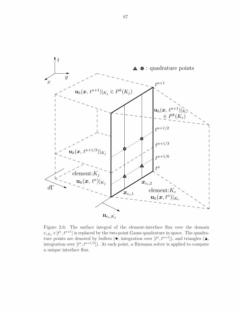
67
t
yx
element:Kj
element:Ke
tn+1
tn+1/2
tn+1/6
tn
uh(x, tn)|Kj
uh(x, tn)|Ke
uh(x, tn+1)|Kj ∈ P k(Kj)
uh(x, tn+1)|Ke
∈ P k(Ke)
dΓxei,1
xei,2
nei,Kj
uh(x, tn+1/3)|Kj
tn+1/3
: quadrature points
Figure 2.6: The surface integral of the element-interface flux over the domainei,Kj
×[tn, tn+1] is replaced by the two-point Gauss quadrature in space. The quadra-ture points are denoted by bullets (•, integration over [tn, tn+1]), and triangles (N,integration over [tn, tn+1/3]). At each point, a Riemann solver is applied to computea unique interface flux.
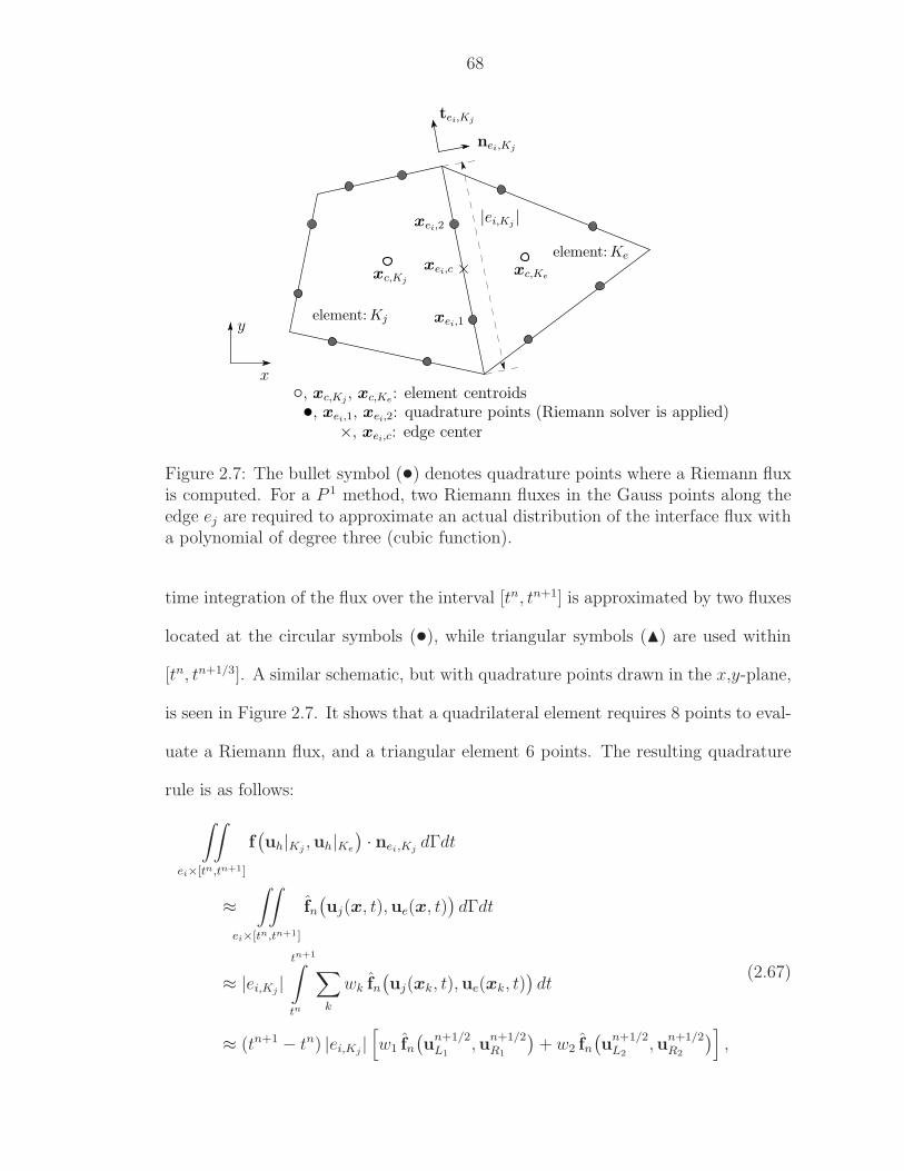
68
xc,Kjxc,Ke
xei,2
xei,1
xei,c
, xc,Kj, xc,Ke: element centroids
•, xei,1, xei,2: quadrature points (Riemann solver is applied)×, xei,c: edge center
x
y
|ei,Kj|
element:Kj
element:Ke
tei,Kj
nei,Kj
Figure 2.7: The bullet symbol (•) denotes quadrature points where a Riemann fluxis computed. For a P 1 method, two Riemann fluxes in the Gauss points along theedge ej are required to approximate an actual distribution of the interface flux witha polynomial of degree three (cubic function).
time integration of the flux over the interval [tn, tn+1] is approximated by two fluxes
located at the circular symbols (•), while triangular symbols (N) are used within
[tn, tn+1/3]. A similar schematic, but with quadrature points drawn in the x,y-plane,
is seen in Figure 2.7. It shows that a quadrilateral element requires 8 points to eval-
uate a Riemann flux, and a triangular element 6 points. The resulting quadrature
rule is as follows:
∫∫
ei×[tn,tn+1]
f(uh|Kj
,uh|Ke
)· nei,Kj
dΓdt
≈∫∫
ei×[tn,tn+1]
fn(uj(x, t),ue(x, t)
)dΓdt
≈ |ei,Kj|
tn+1∫
tn
∑
k
wk fn(uj(xk, t),ue(xk, t)
)dt
≈ (tn+1 − tn) |ei,Kj|[w1 fn
(u
n+1/2L1
,un+1/2R1
)+ w2 fn
(u
n+1/2L2
,un+1/2R2
)],
(2.67)
69
where the weights at Gauss points are
w1 = w2 =1
2, (2.68)
|ei,Kj| is the length of the edge ei belonging to the element Kj, and the input
quantities of the Riemann solver are
un+1/2L1
= uh
(xei,1, tn+1/2
)|Kj
, un+1/2L2
= uh
(xei,2, tn+1/2
)|Kj
, (2.69a)
un+1/2R1
= uh
(xei,1, tn+1/2
)|Ke, u
n+1/2R2
= uh
(xei,2, tn+1/2
)|Ke. (2.69b)
The x-,y-coordinates of Gauss points xei,1, xei,2 are computed by
xei,1 = xei,c −|ei,Kj
|2√
3tei,Kj
, (2.70a)
xei,2 = xei,c +|ei,Kj
|2√
3tei,Kj
, (2.70b)
where tei,Kjis the unit vector tangential to the edge ej of the element Kj. Other
quadrature points denoted by triangular symbols correspond to a time integral
over [tn, tn+1/3]. This integral is necessary to obtain the intermediate solution
uh(x, tn+1/3), used for the volume integral of the source term.
Hancock’s Predictor Step
So far, the interface flux has been replaced by a Riemann solver, and the sur-
face integral has been approximated by a Gaussian quadrature. To complete the
approximation of the surface integral, the last thing we need to specify is how to
compute the input quantities u(xedge, tn+1/2) for a Riemann solver, associated to
the half-time level tn+1/2. Based on Hancock’s observation, flow quantities evolve
over the half time step without any interactions with neighbors. Hence, from the
update formula for conserved variables (2.64a) on page 64, element-face interactions
70
can be removed:
un+1/2j = un
j − 1
2|Aj|∑
ei∈∂Kj
∫∫
ei×T ′
f(uh(xei
, t)|Kj
)· nei,Kj
dΓdt
+1
2|Aj|
∫∫
Kj×T ′
1
ǫs(uh(x, t)
)dxdt, (2.71)
where T ′ := [tn, tn+1/2], and the flux tensor f is simply evaluated from the solution
at each quadrature point xeiof the element Kj , obtained by (2.58a) on page 61.
The predictor step (2.71) to compute the cell-average quantities at time tn+1/2 can
be further simplified with the approximations in evaluating the flux integral at time
tn. As for the source term, since we are considering a stiff case, that is ǫ ≪ O(1),
an L-stable method for the temporal integration is preferable even in the predictor
step. The simplest one is the backward Euler method, hence the source integral is
evaluated at tn+1/2; then (2.71) becomes
un+1/2j = un
j − ∆t
2|Aj|∑
ei∈∂Kj
∫
ei
f(uh(xei
, tn)|Kj
)· nei,Kj
dΓ
+∆t
2|Aj|
∫
Kj
1
ǫs(uh(x, tn+1/2)
)dx, (2.72)
where
uh(xei, tn) = un
j + φnj
(∆xu
n
j , ∆yun
j
)· (xei
− xc,Kj). (2.73)
Here xc,Kjis the centroid of the element Kj , and φn
j is a gradient limiter such
as the TVB corrected minmod function by Cockburn and Shu [CS98]. The mim-
mod treatment of computing the slope from a few candidates can be replaced by
the Barth–Jespersen limiter [BJ89, Bar90], which is a multidimensional extension
of the one-dimensional double-minmod limiter [vL77], or the Venkatakrishnan lim-
iter [Ven95], which is the extension of the Van Alvada limiter [vAvLR82].
71
The latest development in limiters for DG methods is the hierarchical recon-
struction due to Liu [LSTZ07], based on the moment limiter originally developed
by Biswas et al. [BDF94]. The approach reduces the limiting process a high-degree
polynomial to multiple limiting of piecewise linear functions. Thus, once a ‘good’
limiter for solution in P 1 is developed, the limiter can be applied to any higher-
degree polynomial hierarchically. Huynh’s new P 1 limiter seems to be a good can-
didate [Huy06b], but it still needs to be extended to an unstructured grid.
Once the predicted cell-average quantity uk+1/2j at the element Kj is obtained,
the distribution of the solution along the edge ei can be computed by
uh(xei, tn+1/2) = u
n+1/2j + φn
j
(∆xu
n
j , ∆yun
j
)· (xei
− xc,Kj). (2.74)
Note that the slope variables ∆xun
j , ∆yun
j are still associated with the time tn. In
order to make the time integration of the source term point-implicit, the spatial
integral of the source term is evaluated with the solution at just one Gauss point,
(xei, tn+1/2), thus
∫
Kj
1
ǫs(uh(x, tn+1/2)
)dx ≈ |Aj|
ǫs(uh(xei
, tn+1/2)). (2.75)
Inserting the above equation into (2.72) leads to the following implicit predictor
step for the input value of a Riemann solver:
uh(xei, tn+1/2) = un
j − ∆t
2|Aj|∑
ei∈∂Kj
∫
ei
f(uh(xei
, tn)|Kj
)· nei,Kj
dΓ
+ φnj
(∆xu
n
j , ∆yun
j
)· (xei
− xc,Kj) +
∆t
2ǫs(uh(xei
, tn+1/2)). (2.76)
Similar to the 1-D case, this predictor step is often based on the primitive variables
w instead of the conserved ones. Typically, the primitive form provides a linear
source term1
ǫ(w)s(w) = Qww, and the above implicit formula can be rewritten
72
as an explicit predictor. This can be achieved by the following two steps. At first,
the conserved quantity at a particular Gauss point xeiis computed without the
influence of the source term,
uh(xei, tn+1/2) = un
j − ∆t
2|Aj|∑
ei∈∂Kj
∫
ei
f(uh(xei
, tn)|Kj
)· nei,Kj
dΓ
+ φnj
(∆xu
n
j , ∆yun
j
)· (xei
− xc,Kj). (2.77)
Once the predicted conserved quantity uh(xei, tn+1/2) at the Gauss point is obtained,
it is converted to the primitive variable wh(xei, tn+1/2). The reason we do this is
that the P 1 distribution of the solution is only defined in terms of the conserved
variable uh|Kj; the distribution of the primitive variable wh|Kj
in an element is
not even a linear function. Thus, the conversion between conserved and primitive
variables is only valid at a point, but not in the entire element. The final update
formula to obtain the input values for a Riemann solver becomes
wh(xei, tn+1/2) = wh(xei
, tn+1/2) +∆t
2ǫs(wh(xei
, tn+1/2)), (2.78)
and in the case of a linear source,1
ǫ(w)s(w) = Qww, with a constant relaxation
time, ǫ(w) = constant, we have
wh(xei, tn+1/2) =
[I − ∆t
2Qw
]−1
w(xeitn+1/2). (2.79)
If the relaxation time depends on the solution, as in the 10-moment equations,
an iterative method must be applied to solve the implicit formula in the primitive
form (2.78), or conserved form (2.76); the Newton–Raphson method is sufficient.
An alternative is treating the whole predictor step in the primitive form:
wh(xei, tn+1/2) = w(xc,Kj
, tn) − ∆t
2
(Aw ∆xw
nj + Bw ∆yw
nj
)
+ φnj (∆xw
nj , ∆yw
nj ) · (x − xc,Kj
) +∆t
2ǫs(wh(xei
, tn+1/2)), (2.80)
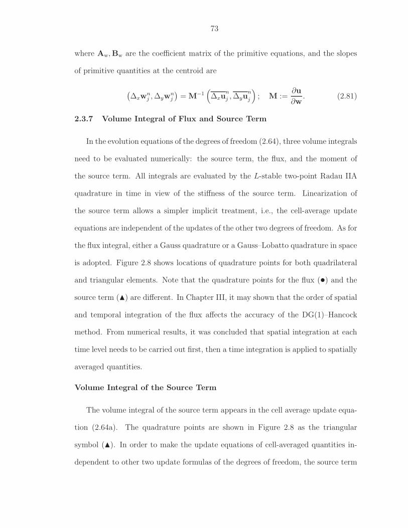
73
where Aw,Bw are the coefficient matrix of the primitive equations, and the slopes
of primitive quantities at the centroid are
(∆xw
nj , ∆yw
nj
)= M−1
(∆xu
n
j , ∆yun
j
); M :=
∂u
∂w. (2.81)
2.3.7 Volume Integral of Flux and Source Term
In the evolution equations of the degrees of freedom (2.64), three volume integrals
need to be evaluated numerically: the source term, the flux, and the moment of
the source term. All integrals are evaluated by the L-stable two-point Radau IIA
quadrature in time in view of the stiffness of the source term. Linearization of
the source term allows a simpler implicit treatment, i.e., the cell-average update
equations are independent of the updates of the other two degrees of freedom. As for
the flux integral, either a Gauss quadrature or a Gauss–Lobatto quadrature in space
is adopted. Figure 2.8 shows locations of quadrature points for both quadrilateral
and triangular elements. Note that the quadrature points for the flux (•) and the
source term (N) are different. In Chapter III, it may shown that the order of spatial
and temporal integration of the flux affects the accuracy of the DG(1)–Hancock
method. From numerical results, it was concluded that spatial integration at each
time level needs to be carried out first, then a time integration is applied to spatially
averaged quantities.
Volume Integral of the Source Term
The volume integral of the source term appears in the cell average update equa-
tion (2.64a). The quadrature points are shown in Figure 2.8 as the triangular
symbol (N). In order to make the update equations of cell-averaged quantities in-
dependent to other two update formulas of the degrees of freedom, the source term
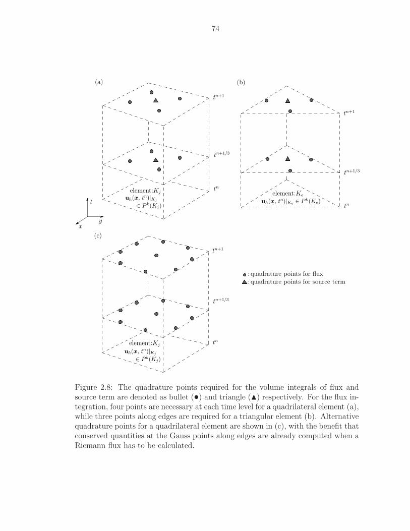
74
element:Kj element:Ke
uh(x, tn)|Ke ∈ P k(Ke)
tn+1
tn
tn+1/3
(b)
tn+1
tn
tn+1/3
uh(x, tn)|Kj
∈ P k(Kj)
element:Kj
tn+1
tn
tn+1/3
uh(x, tn)|Kj
∈ P k(Kj)
(c)
(a)
: quadrature points for flux: quadrature points for source term
t
yx
Figure 2.8: The quadrature points required for the volume integrals of flux andsource term are denoted as bullet (•) and triangle (N) respectively. For the flux in-tegration, four points are necessary at each time level for a quadrilateral element (a),while three points along edges are required for a triangular element (b). Alternativequadrature points for a quadrilateral element are shown in (c), with the benefit thatconserved quantities at the Gauss points along edges are already computed when aRiemann flux has to be calculated.
75
is linearized such that
1
ǫs(uh(x, t)) ≈ 1
ǫ(uj(t))s(uj(t)
)+Q
(uj(t)
) (∆xuj(t), ∆yuj(t)
)·(x−xc,Kj
), (2.82)
where Q(u) =∂(s/ǫ)
∂u. By approximating the above linearization, integration in
space is evaluated analytically, and the volume integral can be simplified together
with the two-point Radau IIA method such that
∫∫
Kj×T
1
ǫs(uh(x, t)
)dxdt ≈ |Aj|
∫
T
1
ǫs(uj(t)
)dt
≈ |Aj|∆t
[3
4
s(un+1/3j )
ǫ(un+1/3j )
+1
4
s(un+1j )
ǫ(un+1j )
]. (2.83)
Volume Integral of the Flux
Volume integrals of the flux appear in the update formula of the slope quanti-
ties (2.64b). The space-time volume integral is first approximated by the two-point
Radau IIA quadrature in time:
∫∫
Kj×T
f(uh(x, t)) dxdt ≈ ∆t
∫
Kj
[3
4f(u(x, tn+1/3)
)+
1
4f(u(x, tn+1)
)]dx. (2.84)
The next step is quadrature of the flux in space at the time levels tn+1/3, tn+1. Since
the shape of an element can be any polygon, a coordinate transformation from the
global (physical) coordinate, x = (x, y), to the local (computational) coordinate,
ξ = (ξ, η), is necessary. In this section, we keep the formulation in general form to
make it valid for both quadrilateral and triangular elements. Let J be the Jacobian
matrix of the coordinate transformation from ξ to x, thus J :=∂x
∂ξ∈ R2×2, then
the integration over the domain Kj can be transform to the local domain Kj :=
[−1, 1] × [−1, 1] such that
∫
Kj
f(u(x, t)) dx =
∫
Kj
f(u(ξ, t))|J(ξ)| dξ, (2.85)
76
where |J(ξ)| is the Jacobian determinant. In the case of a triangular element, the
Jacobian determinant is constant and equivalent to the area of a triangle, which
further simplifies the above quadrature. Conversely, for a quadrilateral element,
both the flux and Jacobian determinant at a quadrature point in the local domain
Kj have to be evaluated simultaneously. The quadrature points for quadrilateral and
triangular elements are indicated in Figure 2.8(a) and (b) by the bullet symbol (•).
Cockburn and Shu propose to recycle extrapolated quantities already computed for
a Riemann solver [CS98, p. 206]. This leads to the nine-point quadrature shown
in Figure 2.8(c). The only extra computational work is computing the flux at the
centroid of the local element Kj . Finally, the volume integral of the flux is replaced
by quadrature:
∫∫
Kj×T
f(uh(x, t)) dxdt ≈ ∆t∑
i
wi|J(ξi)|[3
4f(u(ξi, t
n+1/3)) +1
4f(u(ξi, t
n+1))
],
(2.86a)
where wi are the weights at Gauss points. The detailed implementation of the
coordinate transformation for quadrilateral and triangular elements are provided in
Appendix A on page 343.
Volume Integral of the Moment of the Source Term
The volume integral of the moment of the source term appears in the evolution
equations of slope quantities (2.64b) on page 64. Following the procedure taken for
the source-term volume integral, the source term linearization (2.82) is assumed.
Hence, the spatial integration is done analytically, while the two-point Radau IIA
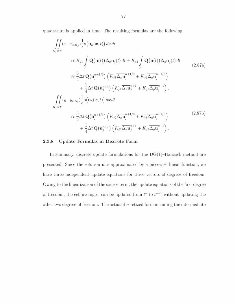
77
quadrature is applied in time. The resulting formulas are the following:
∫∫
Kj×T
(x−xc,Kj)1
ǫs(uh(x, t)
)dxdt
≈ Kj1
∫
T
Q(u(t)
)∆xuj(t) dt + Kj2
∫
T
Q(u(t)
)∆yuj(t) dt
≈ 3
4∆tQ
(u
n+1/3j
) (Kj1∆xu
n+1/3
j + Kj2∆yun+1/3
j
)
+1
4∆tQ
(un+1
j
) (Kj1∆xu
n+1
j + Kj2∆yun+1
j
),
(2.87a)
∫∫
Kj×T
(y−yc,Kj)1
ǫs(uh(x, t)
)dxdt
≈ 3
4∆tQ
(u
n+1/3j
) (Kj2∆xu
n+1/3
j + Kj3∆yun+1/3
j
)
+1
4∆tQ
(un+1
j
) (Kj2∆xu
n+1
j + Kj3∆yun+1
j
).
(2.87b)
2.3.8 Update Formulas in Discrete Form
In summary, discrete update formulations for the DG(1)–Hancock method are
presented. Since the solution u is approximated by a piecewise linear function, we
have three independent update equations for three vectors of degrees of freedom.
Owing to the linearization of the source term, the update equations of the first degree
of freedom, the cell averages, can be updated from tn to tn+1 without updating the
other two degrees of freedom. The actual discretized form including the intermediate
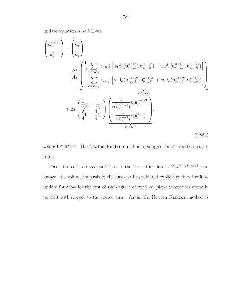
78
update equation is as follows:
un+1/3j
un+1j
=
unj
unj
− ∆t
|Aj |
1
3
∑
ei∈∂Kj
|ei,Kj|[w1 fn
(u
n+1/6ei,1,L ,u
n+1/6ei,1,R
)+ w2 fn
(u
n+1/6ei,2,L ,u
n+1/6ei,2,R
)]
∑
ei∈∂Kj
|ei,Kj|[w1 fn
(u
n+1/2ei,1,L ,u
n+1/2ei,1,R
)+ w2 fn
(u
n+1/2ei,2,L ,u
n+1/2ei,2,R
)]
︸ ︷︷ ︸explicit
+ ∆t
5
12I − 1
12I
3
4I
1
4I
1
ǫ(un+1/3j )
s(un+1/3j )
1
ǫ(un+1j )
s(un+1j )
︸ ︷︷ ︸implicit
,
(2.88a)
where I ∈ Rm×m. The Newton–Raphson method is adopted for the implicit source
term.
Once the cell-averaged variables at the three time levels, tn, tn+1/3, tn+1, are
known, the volume integrals of the flux can be evaluated explicitly; then the final
update formulas for the rest of the degrees of freedom (slope quantities) are only
implicit with respect to the source term. Again, the Newton–Raphson method is
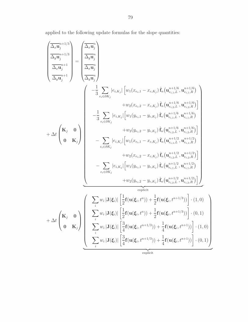
79
applied to the following update formulas for the slope quantities:
∆xun+1/3
j
∆yun+1/3
j
∆xun+1
j
∆yun+1
j
=
∆xun
j
∆yun
j
∆xun
j
∆yun
j
+ ∆t
Kj 0
0 Kj
−1
3
∑
ei∈∂Kj
|ei,Kj|[w1(xei,1 − xc,Kj
) fn(u
n+1/6ei,1,L ,u
n+1/6ei,1,R
)
+w2(xei,2 − xc,Kj) fn(u
n+1/6ei,2,L ,u
n+1/6ei,2,R
)]
−1
3
∑
ei∈∂Kj
|ei,Kj|[w1(yei,1 − yc,Kj
) fn(u
n+1/6ei,1,L ,u
n+1/6ei,1,R
)
+w2(yei,2 − yc,Kj) fn(u
n+1/6ei,2,L ,u
n+1/6ei,2,R
)]
−∑
ei∈∂Kj
|ei,Kj|[w1(xei,1 − xc,Kj
) fn(u
n+1/2ei,1,L ,u
n+1/2ei,1,R
)
+w2(xei,2 − xc,Kj) fn(u
n+1/2ei,2,L ,u
n+1/2ei,2,R
)]
−∑
ei∈∂Kj
|ei,Kj|[w1(yei,1 − yc,Kj
) fn(u
n+1/2ei,1,L ,u
n+1/2ei,1,R
)
+w2(yei,2 − yc,Kj) fn(u
n+1/2ei,2,L ,u
n+1/2ei,2,R
)]
︸ ︷︷ ︸explicit
+ ∆t
Kj 0
0 Kj
∑
i
wi |J(ξi)|[1
2f(u(ξi, t
n)) +1
2f(u(ξi, t
n+1/3))
]· (1, 0)
∑
i
wi |J(ξi)|[1
2f(u(ξi, t
n)) +1
2f(u(ξi, t
n+1/3))
]· (0, 1)
∑
i
wi |J(ξi)|[3
4f(u(ξi, t
n+1/3)) +1
4f(u(ξi, t
n+1))
]· (1, 0)
∑
i
wi |J(ξi)|[3
4f(u(ξi, t
n+1/3)) +1
4f(u(ξi, t
n+1))
]· (0, 1)
︸ ︷︷ ︸explicit
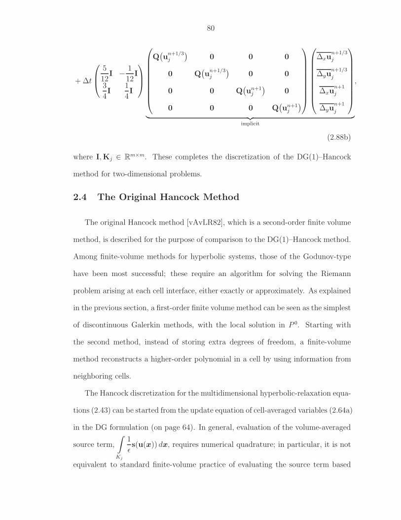
80
+ ∆t
5
12I − 1
12I
3
4I
1
4I
Q(u
n+1/3j
)0 0 0
0 Q(u
n+1/3j
)0 0
0 0 Q(un+1
j
)0
0 0 0 Q(un+1
j
)
∆xun+1/3
j
∆yun+1/3
j
∆xun+1
j
∆yun+1
j
︸ ︷︷ ︸implicit
,
(2.88b)
where I,Kj ∈ Rm×m. These completes the discretization of the DG(1)–Hancock
method for two-dimensional problems.
2.4 The Original Hancock Method
The original Hancock method [vAvLR82], which is a second-order finite volume
method, is described for the purpose of comparison to the DG(1)–Hancock method.
Among finite-volume methods for hyperbolic systems, those of the Godunov-type
have been most successful; these require an algorithm for solving the Riemann
problem arising at each cell interface, either exactly or approximately. As explained
in the previous section, a first-order finite volume method can be seen as the simplest
of discontinuous Galerkin methods, with the local solution in P 0. Starting with
the second method, instead of storing extra degrees of freedom, a finite-volume
method reconstructs a higher-order polynomial in a cell by using information from
neighboring cells.
The Hancock discretization for the multidimensional hyperbolic-relaxation equa-
tions (2.43) can be started from the update equation of cell-averaged variables (2.64a)
in the DG formulation (on page 64). In general, evaluation of the volume-averaged
source term,
∫
Kj
1
ǫs(u(x)) dx, requires numerical quadrature; in particular, it is not
equivalent to standard finite-volume practice of evaluating the source term based
81
on the cell-average, s(u(xj)). For instance, in the 1-D case,
sj(u) : =1
∆x
∫
Ij
s(u(x)) dx
= s(uj) + O(∆x2
). (2.89)
In a second-order accurate method such as described below, though, the average
source term sj(u) can be replaced by s(uj). Similarly, the spatial integral along
edges of an element can be approximated by the midpoint rule; the interface flux
at the element ei is evaluated at the edge center xei,c such that
∫∫
ei×T
f(uh|Kj
,uh|Ke
)· nei,Kj
dΓdt ≈ |ei,Kj|∫
T
fn(uj(xei,c, t),ue(xei,c, t)
)dt, (2.90)
where fn is a Riemann flux outward of Kj and normal to the edge ej , and |ei,Kj| is the
length of the edge ei belonging to the element Kj . Figure 2.9 shows the quadrature
points (midpoint rule) where a Riemann solver is applied. Consequently, finite-
volume methods of second-order accuracy in space can be written in fully discrete
form as
un+1j = un
j − 1
|Aj|∑
ei∈∂Kj
|ei,Kj
|∫
T
fn(uj(xei,c, t),ue(xei,c, t)
)dt
+
∫
T
1
ǫs(uj(t)) dt.
(2.91)
Note that time integrations of the flux and source term along the time domain
T := [tn, tn+1] have not been specified yet. Second-order accuracy in space and
time is achieved by introducing linear subcell distributions and evaluating fluxes
and source terms halfway during the time step:
∫
T
fn(uj(xei,c, t),ue(xei,c, t)
)dt ≈ ∆t fn
(uj(xei,c, t
n+1/2),ue(xei,c, tn+1/2)
), (2.92a)
∫
T
1
ǫs(uj(t)) dt ≈ ∆t
ǫs(uj(t
n+1/2)). (2.92b)
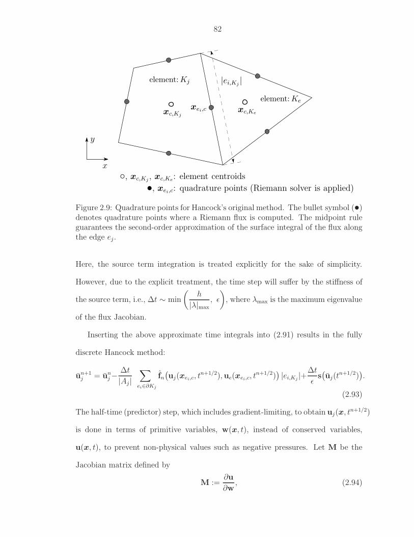
82
xc,Kjxc,Ke
xei,c
, xc,Kj, xc,Ke: element centroids
•, xei,c: quadrature points (Riemann solver is applied)
x
y
|ei,Kj|element:Kj
element:Ke
Figure 2.9: Quadrature points for Hancock’s original method. The bullet symbol (•)denotes quadrature points where a Riemann flux is computed. The midpoint ruleguarantees the second-order approximation of the surface integral of the flux alongthe edge ej .
Here, the source term integration is treated explicitly for the sake of simplicity.
However, due to the explicit treatment, the time step will suffer by the stiffness of
the source term, i.e., ∆t ∼ min
(h
|λ|max
, ǫ
), where λmax is the maximum eigenvalue
of the flux Jacobian.
Inserting the above approximate time integrals into (2.91) results in the fully
discrete Hancock method:
un+1j = un
j −∆t
|Aj |∑
ei∈∂Kj
fn(uj(xei,c, t
n+1/2),ue(xei,c, tn+1/2)
)|ei,Kj
|+∆t
ǫs(uj(t
n+1/2)).
(2.93)
The half-time (predictor) step, which includes gradient-limiting, to obtain uj(x, tn+1/2)
is done in terms of primitive variables, w(x, t), instead of conserved variables,
u(x, t), to prevent non-physical values such as negative pressures. Let M be the
Jacobian matrix defined by
M :=∂u
∂w, (2.94)
83
then the two-dimensional hyperbolic-relaxation equations can be reformulated in
the primitive form:
∂w
∂t+ Aw
∂w
∂x+ Bw
∂w
∂y= M−11
ǫs(w), (2.95)
where Aw,Bw ∈ Rm×m are the coefficient matrices of the primitive equations 1
obtained by a similarity transformation of the flux Jacobian:
Aw,Bw := M−1
(∂f(u)
∂u
)M; f ∈ R
m×2. (2.96)
When the 10-moment equations are considered, owing to its simple structure, the
source term is not affected by the variable transformation: M−1 1
ǫs ≡ 1
ǫs. Since the
divergence theorem can not be applied to the primitive form, we discretize (2.95)
by finite-differencing. Applying the forward Euler method in time, the primitive
quantities at the half time step, wn+1/2j , are approximated by
wn+1/2j = wn
j − ∆t
2
(Aw ∆xw
nj + Bw ∆yw
nj
)+
∆t
2ǫs(wn
j ), (2.97)
where the gradients of the primitive variables, ∇wnj = (∆xw
nj , ∆yw
nj ), are ob-
tained by either the Green–Gauss formula [BF90] or solving a least-square prob-
lems [Bar93, OGvA02] involving data from all adjacent cells. In general, the least-
squares gradient reconstruction is more robust than the Green–Gauss contour inte-
gral, yet various ways of weighting residuals are possible in the former method, and
the unweighted approach this is often taken is not even the best [Mav07].
Once primitive variables at half-time are obtained, interface fluxes are computed
by solving Riemann problems. Finally, the full-time (corrector) step to update
1The resulting matrix An should not be called as the primitive Jacobian since the definition ofa Jacobian matrix is the derivative of one vector to another one. The reader is referred to helpfulhints in [vL06] for preventing misuse of terminologies.
84
conservative variables can be written as
un+1j = un
j −∆t
|Aj |∑
ei∈∂Kj
fn(wj(xei,c, t
n+1/2), we(xei,c, tn+1/2)
)|ei,Kj
|+∆t
ǫs(wj(t
n+1/2)),
(2.98)
where the primitive quantities, wn+1/2j , associated with the centroid of a cell, are
linearly extrapolated to the midpoint xei,c of the edge ei by
wj(x, tn+1/2) = wn+1/2j + φi (∇wn
j ) · (x − xc,Kj). (2.99)
Here φi is a gradient limiter such as the double-minmod limiter [Bar90], and xc,Kj
is the centroid of cell Kj . For details of implementation one is referred to [DZ93,
pp. 49–57]. Note that the slope quantities, ∇wnj , are used for the reconstruction
step; ideally, slopes associated with the time level tn+1/2 need to be computed, yet
old slopes are sufficient for a second-order method.
2.5 Semi-Discrete Methods
The DG(1)–Hancock and Hancock methods introduced in the previous sections
are fully discrete methods. This means that the spatial and temporal derivatives are
discretized simultaneously. The other approach to discretizing hyperbolic-relaxation
equations (2.1) is based on the method-of-lines (MOL), which decouples the spatial
and temporal discretizations. The advantages of adopting an MOL are the simpli-
fication of the design of a scheme, flexibility to combine a suitable spatial and tem-
poral methods, and ease of implementation. While general-purpose semi-discrete
finite-difference, finite-volume, or discontinuous Galerkin methods are employed as
spatial discretizations, a number of time discretizations (ODE solvers) have been
developed specifically for hyperbolic-relaxation equations.
85
2.5.1 Time Integration with a Stiff Source Term
When a semi-discrete method is considered, the 1-D hyperbolic-relaxation equa-
tions can be written in the form:
∂uj(t)
∂t= −∂f(uj(t))
∂x+
1
ǫs(uj(t)), (2.100)
where the solution uj is still a continuous function in time. Due to the stiffness intro-
duced by the relaxation time ǫ in the source term, the source term needs to be treated
implicitly for stability. Conversely, the flux is evaluated explicitly. One of the dif-
ficulties in designing such a method is that when the flow is in equilibrium, thus
ǫ → 0, the method has to be consistent with the hyperbolic conservation laws (2.2)
at the discretization level. This property guarantees that a underresolved method
correctly captures the macroscopic behavior. Jin named such schemes asymptotic
preserving (AP) [Jin99]. Numerous methods have been proposed to achieve the AP
property [Jin95, CJR97, Jin99, LRR00, Rus02]. These methods are summarized as
the Butcher array in [PR03].
Among the family of these Runge–Kutta methods, Pareschi and Russo ex-
tend the implicit-explicit (IMEX) Runge–Kutta method, originally developed for
advection-diffusion problems [ARS97, ARW95], to hyperbolic-relaxation equations
[PR05]. The methods utilize an explicit, strongly-stability-preserving (SSP) method
for the flux, and an L-stable, diagonally implicit Runge–Kutta method for the source
term. The methods are shown to possess the AP property at the equilibrium limit.
They use the notation IMEX–SSPk(s, σ, p) where k is the order of the SSP scheme,
s the number of states of the implicit method, σ the number of stages of the ex-
plicit method, and p the order of the IMEX method. Here, we adopt a second-order
IMEX Runge–Kutta method: IMEX–SSP2(3,3,2) as the time integration for the
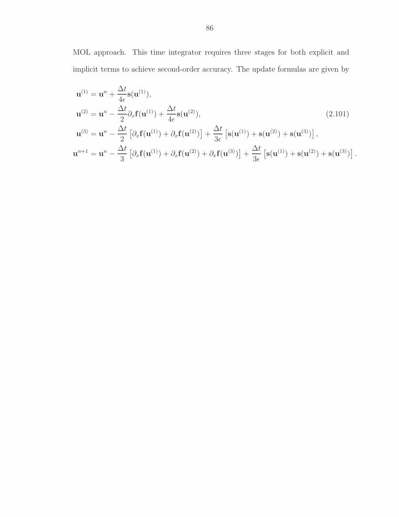
86
MOL approach. This time integrator requires three stages for both explicit and
implicit terms to achieve second-order accuracy. The update formulas are given by
u(1) = un +∆t
4ǫs(u(1)),
u(2) = un − ∆t
2∂xf(u
(1)) +∆t
4ǫs(u(2)), (2.101)
u(3) = un − ∆t
2
[∂xf(u
(1)) + ∂xf(u(2))]+
∆t
3ǫ
[s(u(1)) + s(u(2)) + s(u(3))
],
un+1 = un − ∆t
3
[∂xf(u
(1)) + ∂xf(u(2)) + ∂xf(u
(3))]+
∆t
3ǫ
[s(u(1)) + s(u(2)) + s(u(3))
].
CHAPTER III
ANALYSIS FOR 1-D AND 2-D LINEAR
ADVECTION EQUATIONS
3.1 Introduction
In this chapter, a Fourier analysis is employed to uncover the linear proper-
ties of methods for hyperbolic conservation laws without source terms; hyperbolic-
relaxation systems will be analyzed in Chapter IV. The analysis is also called a ‘Von
Neumann analysis’ named after John von Neumann, who originally introduced the
analysis for parabolic differential equations [vNR47, vNR63]. The actual applica-
tions of the analysis can be found in many textbooks [RM67, TAP97]. The analysis
shows the order of accuracy, the dominant numerical dissipation/dispersion errors
for the low-frequency mode, and the linear stability of a method. Note that the as-
sumptions required for a Fourier analysis are uniform grids and periodic boundary
conditions. The dimensionless 1-D and 2-D linear advection equations,
∂tu + r∂xu = 0, |r| ≤ 1, (3.1a)
∂tu + r∂xu + s∂yu = 0, |r|, |s| ≤ 1, (3.1b)
are considered as the model equations. Here, the normalization is rather uncommon.
The advection speed is normalized by the larger ‘frozen’ wave speed (= 1) arising
87
88
further on in hyperbolic-relaxation systems. The motivation of this normalization
will be clear once hyperbolic-relaxation systems are considered in Chapter IV.
The Courant number, ν, is defined by the dimensionless frozen wave speed, 1,
instead of the advection speed, r, thus
ν := 1∆t
∆x, ∆x, ∆t ∈ R
+. (3.2)
Again, this definition is rather uncommon. Conventionally, the Courant number for
a linear advection equation is defined by
ν := r∆t
∆x, (3.3)
where the advection speed, r, is normalized by the spatial and temporal scales.
To make the analysis consistent with the results later presented for the linear
hyperbolic-relaxation equations, we adopt ν as the Courant number here. The
conventional expression can be recovered by substituting
rν = ν. (3.4)
Recall that, for a linear advection equation, both the upwind moment scheme
(with Gauss–Lobatto quadrature for the volume integral) and the proposed method
(with Gauss–Radau quadrature) are identical to Van Leer’s scheme III [vL77]. The
upwind moment method (DG(1)–Hancock) is compared with three other method-
ologies: a semi-discrete high-resolution Godunov method (HR) with method-of-lines
(MOL) or Hancock time integration, and a DG(1)–MOL method. These methods
can be regarded as the combination of a spatial and a temporal discretization, and
are tabulated in Table 3.1. Here, we adopt the notations HRs and RKs, where s
is the order of accuracy, and DG(k) where k is the degree of the polynomial basis.
A Fourier analysis for the 1-D advection equation shows that the upwind moment
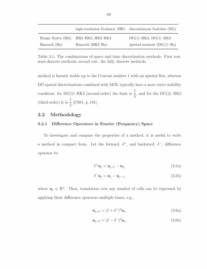
89
high-resolution Godunov (HR) discontinuous Galerkin (DG)
Runge–Kutta (RK) HR2–RK2, HR2–RK3 DG(1)–RK2, DG(1)–RK3
Hancock (Ha) Hancock (HR2–Ha) upwind moment (DG(1)–Ha)
Table 3.1: The combinations of space and time discretization methods. First row:semi-discrete methods; second row: the fully discrete methods.
method is linearly stable up to the Courant number 1 with an upwind flux, whereas
DG spatial discretizations combined with MOL typically have a more strict stability
condition: for DG(1)–RK2 (second-order) the limit is1
3, and for the DG(2)–RK3
(third-order) it is1
5[CS01, p. 191].
3.2 Methodology
3.2.1 Difference Operators in Fourier (Frequency) Space
To investigate and compare the properties of a method, it is useful to write
a method in compact form. Let the forward, δ+, and backward, δ−, difference
operator be
δ+uj = uj+1 − uj, (3.5a)
δ−uj = uj − uj−1, (3.5b)
where uj ∈ Rn. Then, translation over any number of cells can be expressed by
applying these difference operators multiple times, e.g.,
uj+2 = (I + δ+)2uj, (3.6a)
uj−2 = (I − δ−)2uj , (3.6b)
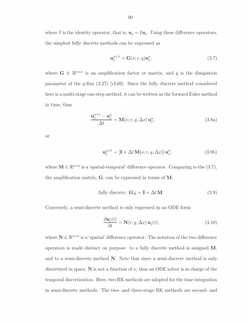
90
where I is the identity operator, that is, uj = Iuj . Using these difference operators,
the simplest fully discrete methods can be expressed as
un+1j = G(ν, r, q)un
j , (3.7)
where G ∈ Rn×n is an amplification factor or matrix, and q is the dissipation
parameter of the q-flux (3.27) [vL69]. Since the fully discrete method considered
here is a multi-stage one-step method, it can be written as the forward Euler method
in time, thus
un+1j − un
j
∆t= M(ν, r, q, ∆x)un
j , (3.8a)
or
un+1j = [I + ∆tM(ν, r, q, ∆x)]un
j , (3.8b)
where M ∈ Rn×n is a ‘spatial-temporal’ difference operator. Comparing to the (3.7),
the amplification matrix, G, can be expressed in terms of M:
fully discrete : GM = I + ∆tM. (3.9)
Conversely, a semi-discrete method is only expressed in an ODE form:
∂uj(t)
∂t= N(r, q, ∆x)uj(t), (3.10)
where N ∈ Rn×n is a ‘spatial’ difference operator. The notation of the two difference
operators is made distinct on purpose: to a fully discrete method is assigned M,
and to a semi-discrete method N. Note that since a semi-discrete method is only
discretized in space, N is not a function of ν, thus an ODE solver is in charge of the
temporal discretization. Here, two RK methods are adopted for the time integration
in semi-discrete methods. The two- and three-stage RK methods are second- and
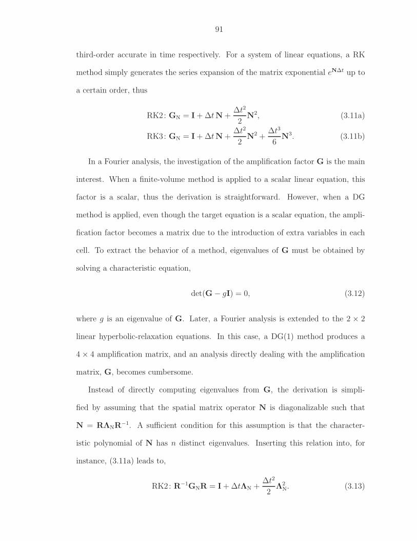
91
third-order accurate in time respectively. For a system of linear equations, a RK
method simply generates the series expansion of the matrix exponential eN∆t up to
a certain order, thus
RK2: GN = I + ∆tN +∆t2
2N2, (3.11a)
RK3: GN = I + ∆tN +∆t2
2N2 +
∆t3
6N3. (3.11b)
In a Fourier analysis, the investigation of the amplification factor G is the main
interest. When a finite-volume method is applied to a scalar linear equation, this
factor is a scalar, thus the derivation is straightforward. However, when a DG
method is applied, even though the target equation is a scalar equation, the ampli-
fication factor becomes a matrix due to the introduction of extra variables in each
cell. To extract the behavior of a method, eigenvalues of G must be obtained by
solving a characteristic equation,
det(G − gI) = 0, (3.12)
where g is an eigenvalue of G. Later, a Fourier analysis is extended to the 2 × 2
linear hyperbolic-relaxation equations. In this case, a DG(1) method produces a
4 × 4 amplification matrix, and an analysis directly dealing with the amplification
matrix, G, becomes cumbersome.
Instead of directly computing eigenvalues from G, the derivation is simpli-
fied by assuming that the spatial matrix operator N is diagonalizable such that
N = RΛNR−1. A sufficient condition for this assumption is that the character-
istic polynomial of N has n distinct eigenvalues. Inserting this relation into, for
instance, (3.11a) leads to,
RK2: R−1GNR = I + ∆tΛN +∆t2
2Λ2
N. (3.13)
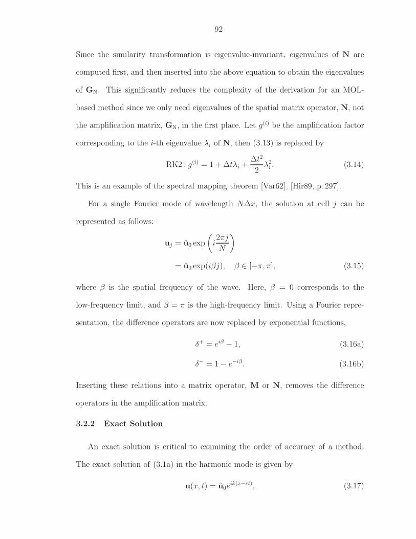
92
Since the similarity transformation is eigenvalue-invariant, eigenvalues of N are
computed first, and then inserted into the above equation to obtain the eigenvalues
of GN. This significantly reduces the complexity of the derivation for an MOL-
based method since we only need eigenvalues of the spatial matrix operator, N, not
the amplification matrix, GN, in the first place. Let g(i) be the amplification factor
corresponding to the i-th eigenvalue λi of N, then (3.13) is replaced by
RK2: g(i) = 1 + ∆tλi +∆t2
2λ2
i . (3.14)
This is an example of the spectral mapping theorem [Var62], [Hir89, p. 297].
For a single Fourier mode of wavelength N∆x, the solution at cell j can be
represented as follows:
uj = u0 exp
(i2πj
N
)
= u0 exp(iβj), β ∈ [−π, π], (3.15)
where β is the spatial frequency of the wave. Here, β = 0 corresponds to the
low-frequency limit, and β = π is the high-frequency limit. Using a Fourier repre-
sentation, the difference operators are now replaced by exponential functions,
δ+ = eiβ − 1, (3.16a)
δ− = 1 − e−iβ. (3.16b)
Inserting these relations into a matrix operator, M or N, removes the difference
operators in the amplification matrix.
3.2.2 Exact Solution
An exact solution is critical to examining the order of accuracy of a method.
The exact solution of (3.1a) in the harmonic mode is given by
u(x, t) = u0eik(x−rt), (3.17)
93
where k is the spatial wave number. The exact amplification factor is obtained by
expressing u(x, t + ∆t) in terms of u(x, t),
u(x, t + ∆t) = u0eik(x−rt)e−irk∆t
= e−irk∆tu(x, t). (3.18)
It shows that the exact amplification factor for the time step ∆t, and the exact
eigenvalue of the spatial discretization operator in (3.10) are given by
gexact = e−irk∆t, (3.19a)
λexact = −irk. (3.19b)
In a Fourier mode, the wave number k is related to the frequency of a wave β by
k =β
∆x, (3.20)
thus the amplification factor and spatial eigenvalue become
gexact(ν, β) = e−irνβ = e−iνβ, (3.21a)
λexact = − ir
∆xβ. (3.21b)
A good understanding of the properties of a method is obtained by rewriting an
amplification factor in the polar form. An amplification factor can be expressed by
the modulus |g| and the phase angle φ ∈ [−π, π] such that
g = |g|eiφ, (3.22)
where
|g| =√
ℜ(g)2 + ℑ(g)2, (3.23a)
φ = arg(g) = arctan
[ℑ(g)
ℜ(g)
]. (3.23b)
94
The modulus represents the dissipation, and the phase angle represents the disper-
sion of a method. For the exact solution, we have
|gexact| = 1, (3.24a)
φexact = −rνβ = −νβ. (3.24b)
Later in an analysis, the low-frequency limit of a Fourier mode is compared with the
exact solution. The exact amplification factor in the low-frequency limit is given by
expanding in the frequency of a wave, β, with the fixed Courant number, rν, thus
gexact(rν, β) = 1 + (−irν)β +1
2(−irν)2β2 +
1
6(−irν)3β3 +
1
24(−irν)4β4 + O
(β5).
(3.25)
3.2.3 Example of the Analysis (First-Order Method)
Before we start analyzing a higher-order method, the first-order method is an-
alyzed to demonstrate a Fourier analysis for both accuracy and stability. Here,
a finite-volume discretization in space, and the forward Euler method in time are
employed for the 1-D linear advection equation (3.1a). The resulting scheme is as
follows:
un+1j − un
j
∆t= − 1
∆x
(fn
j+1/2 − fnj−1/2
), (3.26)
where the linear flux, f(u) = ru, is evaluated at the time level tn at each cell
interface, j ± 1/2. Making the analysis more general, the q-flux [vL69], which
parameterizes the amount of numerical dissipation added into the flux calculation,
95
is employed as the flux function:
f qj+1/2(uL, uR) =
r
2(uL + uR) − q
2(uR − uL), with q =
|r| upwind,
1 Rusanov, HLL1,
∆x
∆tLax–Friedrichs.
(3.27)
The unity value in the Rusanov flux comes from the dimensionless frozen wave speed
which, appears in the linear hyperbolic-relaxation equations. Here, the dissipation
parameter, q, satisfies the inequality,
|r| ≤ q ≤ ∆x
∆t=
1
ν. (3.28)
Thus, it is easily seen that the upwind flux introduces the least numerical dissipation,
whereas the Lax–Friedrichs (LxF) has the most. The first-order approximation of
interface fluxes is given by using the cell-averaged values as input, thus for the
q-flux,
fnj+1/2 = f q
j+1/2(unj , un
j+1), (3.29a)
fnj−1/2 = f q
j−1/2(unj−1, u
nj ). (3.29b)
Here, even though the first-order method (3.26) can be seen as a fully discrete
method, strictly speaking, it is a semi-discrete method combined with the MOL
approach, since the flux formula does not contain time variation. Inserting the
difference equations of fluxes into the update equation, the resulting scheme has the
three-point formula:
un+1j − un
j
∆t= − r
2∆x(un
j+1 − unj−1) +
q
2∆x(un
j+1 − 2unj + un
j−1)
=q − r
2∆xun
j+1 −q
∆xun
j +q + r
2∆xun
j−1. (3.30)
96
Applying the difference operators (3.5) to the above equation leads to the compact
form, thus
un+1j = g1st-orderu
nj
= (1 + ∆t N1st-order) unj , (3.31)
where
N1st-order =q − r
2∆xδ+ − q + r
2∆xδ−, (3.32a)
or for a Fourier mode,
N1st-order =q − r
2∆xeiβ − q
∆x+
q + r
2∆xe−iβ. (3.32b)
Shift Condition
When the upwind flux, q = r, is used, and the Courant number is set to unity,
thus r∆t
∆x= 1, then the spatial difference operator multiplied by the time step, ∆t,
reduces to
∆tN1st-order = −∆t( r
∆xδ−)
= −δ−, (3.33)
which is the exact upwind difference operator. Inserting the above equation into
the update formula (3.31) leads to the exact solution:
un+1j = (1 − δ−)un
j
= unj−1. (3.34)
The property, which a method reduces to the exact solution with unity Courant
number, is called the shift condition, or the unit CFL condition [LeV02, p. 85]. This
property can be found in some fully discrete methods, but almost never in the
high-order semi-discrete methods.
97
Amplification Factor
Once the compact difference form is obtained, replacing the difference operators
δ± by the Fourier mode (3.16) leads to
λ1st-order = − 1
∆x[q(1 − cos β) + ir sin β] , (3.35)
where we explicitly change the notation from N to λ, stating that λ is the eigenvalue
of N. In this example, λ and N are identical, however, when a DG method is
adopted for a scalar linear equation, or any scheme for a system of linear equations,
the difference operator, N, becomes a matrix. In these cases, the characteristic
equation,
det(N − λI) = 0, (3.36)
needs to be solved to obtain eigenvalues of spatial difference operators. Once the
eigenvalue of the spatial difference operator, N, is obtained, the amplification factor,
g, is given by
g1st-order = 1 + ∆tλ1st-order
= 1 − ν [q(1 − cos β) + ir sin β] (3.37a)
= 1 − ν[qr(1 − cos β) + i sin β
]. (3.37b)
To analyze the properties of the method, it is useful to rewrite the amplification
factor in the polar form (3.22), thus
g1st-order = |g1st-order|eiφ1st-order , (3.38)
where
|g1st-order| =
√
1 − 4
[qν − (rν)2 −
((qν)2 − (rν)2
)sin2 β
2
]sin2 β
2, (3.39a)
φ1st-order = arctan
[ −rν sin β
1 − qν(1 − cos β)
]. (3.39b)
98
Accuracy
Typically, we are interested in the behavior of a method in the low-frequency
limit, β ≪ 1. Taking the power-series expansion around β = 0 of the amplification
factor and phase angle leads to
|g1st-order| = 1 − 1
2
[qν − (rν)2
]β2 + O
(β4), (3.40a)
φ1st-order = −rνβ +1
6rν[1 − 3qν + 2(rν)2
]β3 + O
(β5). (3.40b)
The equations (3.40) shows the amount of dissipation (amplitude error) appears
in even orders of β, and the dispersion (phase error) in odd orders. The relative
errors of dissipation and dispersion are obtained by comparing with the exact solu-
tion (3.24) respectively, thus
|g1st-order||gexact|
= 1 + O(β2), (3.41a)
φ1st-order
φexact
= 1 + O(β2). (3.41b)
The overall order of accuracy can be derived by assuming the following form:
gmethod = eλmethod∆t, (3.42)
where λmethod is the eigenvalue containing the information of both spatial and tem-
poral discretizations. This formula assumes that a method has unique exponential
form that includes both spatial and temporal discretization errors in the eigenvalue,
λmethod. Note that λ1st-order is somewhat different with λ1st-order in (3.35) since the
latter contains only the spatial discretization error. Taking the logarithm of the
99
amplification factor leads to
λ1st-order∆t = ln(g1st-order)
= ln|g1st-order| + iφ1st-order
= −irνβ − 1
2
[qν − (rν)2
]β2 +
1
6irν[1 − 3qν + 2(rν)2
]β3 + O
(β4).
(3.43)
The leading error terms are obtained by subtracting the exact eigenvalue (3.21a)
from the discretization method,
λ1st-order∆t − λexact∆t = −1
2
[qν − (rν)2
]β2 +
1
6irν[1 − 3qν + 2(rν)2
]β3 + O
(β4).
(3.44)
To derive the order of accuracy, the frequency, β, is replaced by the wave number, k,
given by (3.20). Then, dividing it by the time step, ∆t, leads to the local truncation
error (LTE) of the method, thus
LTE1st-order = λ1st-order − λexact
= −1
2
(q ∆x − r2 ∆t
)k2 +
ir
6
[1 − 3qν + 2(rν)2
]∆x2k3 + O
(k4),
(3.45)
here we assume the grid size, ∆x, is fixed to guarantee the correct asymptotic
expansion with respect to k. The leading error is the k2-term with coefficients ∆x
and ∆t, thus the method is first-order accurate in space and time.
The relation between λ1st-order and λ1st-order becomes clear after taking the series
expansion of the eigenvalue (3.35). Following the same procedure, the truncation
error of the spatial discretization is given by
λ1st-order − λexact = −1
2q ∆x k2 +
ir∆x2
6k3 + O
(k4), (3.46)
thus the spatial discretization is first-order accurate in space. The identical trun-
cation error is obtained by letting ∆t, ν → 0 in (3.45). This example shows that
100
analyzing the eigenvalue of spatial discretization, λmethod, provides only the order
of accuracy in space. Hence, the eigenvalue, λmethod, defined by (3.42) is necessary
to examine the order of accuracy in both space and time.
The order of accuracy can be also obtained by expanding the amplification
factor (3.37) directly with respect to β:
g1st-order = 1 − irνβ − 1
2qνβ2 +
1
6irνβ3 + O
(β4). (3.47)
Subtracting (3.25) from the above equation leads to the leading error term,
g1st-order − gexact = −1
2
[qν − (rν)2
]β2 +
1
6irν[1 − (rν)2
]β3 + O
(β4). (3.48)
Following the same procedure, replacing β by k, and dividing by ∆t, leads to the
same conclusion. This approach is more straightforward for deriving the order
of accuracy in the low-frequency limit; however, the resulting formula does not
distinguish whether the higher-order error comes from the dissipation or dispersion
any more. This is due to the fact that when (3.42) is expanded,
gmethod = 1 + λ∆t +1
2(λ∆t)2 + O
((λ∆t)3
), (3.49)
and (3.43) is inserted, the (λ∆t)2 term will produce the β3-term which results from
the multiplication of β (dispersion) and β2 (dissipation) terms. Thus, the resulting
formula can not distinguish the error coming from two different sources even though
it has a similar form of (3.43). Nevertheless, the leading error term, β2-term in this
case, is always identical in both approaches.
Stability
The stability of a method can be examined by the modulus of the amplification
factor (3.23a). The necessary and sufficient condition for linear stability is
|g(β, ν)| ≤ 1 for any β ∈ [−π, π]. (3.50)
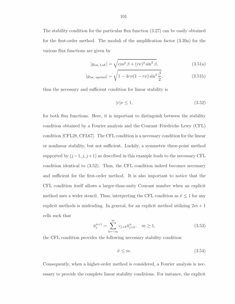
101
The stability condition for the particular flux function (3.27) can be easily obtained
for the first-order method. The moduli of the amplification factor (3.39a) for the
various flux functions are given by
|g1st, LxF| =√
cos2 β + (rν)2 sin2 β, (3.51a)
|g1st, upwind| =
√1 − 4rν(1 − rν) sin2 β
2, (3.51b)
thus the necessary and sufficient condition for linear stability is
|r|ν ≤ 1, (3.52)
for both flux functions. Here, it is important to distinguish between the stability
condition obtained by a Fourier analysis and the Courant–Friedrichs–Lewy (CFL)
condition [CFL28, CFL67]. The CFL condition is a necessary condition for the linear
or nonlinear stability, but not sufficient. Luckily, a symmetric three-point method
supported by (j−1, j, j+1) as described in this example leads to the necessary CFL
condition identical to (3.52). Thus, the CFL condition indeed becomes necessary
and sufficient for the first-order method. It is also important to notice that the
CFL condition itself allows a larger-than-unity Courant number when an explicit
method uses a wider stencil. Thus, interpreting the CFL condition as ν ≤ 1 for any
explicit methods is misleading. In general, for an explicit method utilizing 2m + 1
cells such that
un+1j =
m∑
k=−m
cj+kunj+k, m ≥ 1, (3.53)
the CFL condition provides the following necessary stability condition:
ν ≤ m. (3.54)
Consequently, when a higher-order method is considered, a Fourier analysis is nec-
essary to provide the complete linear stability conditions. For instance, the explicit
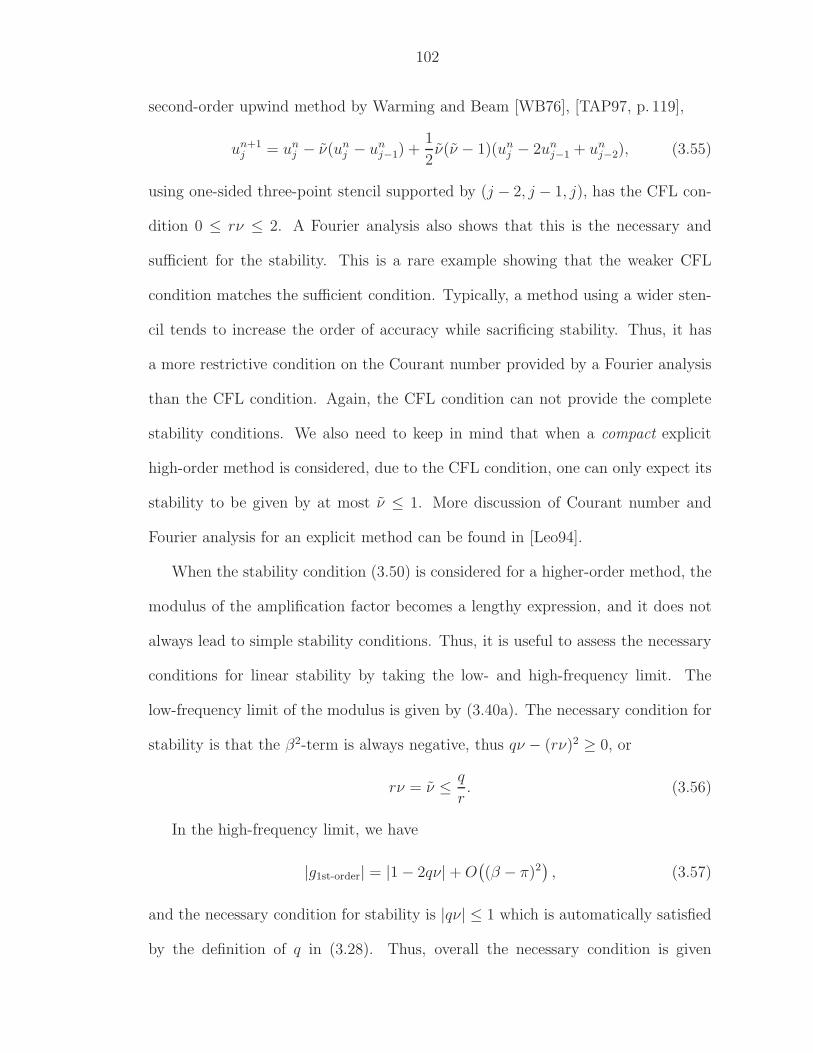
102
second-order upwind method by Warming and Beam [WB76], [TAP97, p. 119],
un+1j = un
j − ν(unj − un
j−1) +1
2ν(ν − 1)(un
j − 2unj−1 + un
j−2), (3.55)
using one-sided three-point stencil supported by (j − 2, j − 1, j), has the CFL con-
dition 0 ≤ rν ≤ 2. A Fourier analysis also shows that this is the necessary and
sufficient for the stability. This is a rare example showing that the weaker CFL
condition matches the sufficient condition. Typically, a method using a wider sten-
cil tends to increase the order of accuracy while sacrificing stability. Thus, it has
a more restrictive condition on the Courant number provided by a Fourier analysis
than the CFL condition. Again, the CFL condition can not provide the complete
stability conditions. We also need to keep in mind that when a compact explicit
high-order method is considered, due to the CFL condition, one can only expect its
stability to be given by at most ν ≤ 1. More discussion of Courant number and
Fourier analysis for an explicit method can be found in [Leo94].
When the stability condition (3.50) is considered for a higher-order method, the
modulus of the amplification factor becomes a lengthy expression, and it does not
always lead to simple stability conditions. Thus, it is useful to assess the necessary
conditions for linear stability by taking the low- and high-frequency limit. The
low-frequency limit of the modulus is given by (3.40a). The necessary condition for
stability is that the β2-term is always negative, thus qν − (rν)2 ≥ 0, or
rν = ν ≤ q
r. (3.56)
In the high-frequency limit, we have
|g1st-order| = |1 − 2qν| + O((β − π)2
), (3.57)
and the necessary condition for stability is |qν| ≤ 1 which is automatically satisfied
by the definition of q in (3.28). Thus, overall the necessary condition is given
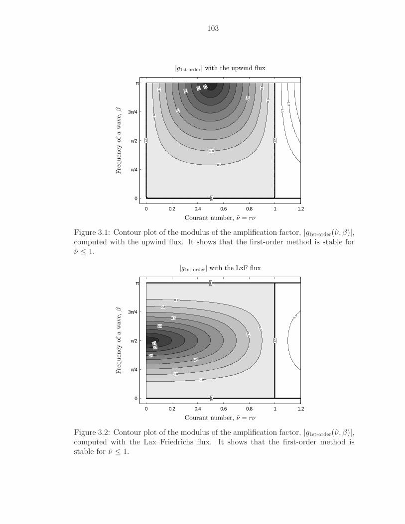
103
0 0.2 0.4 0.6 0.8 1 1.2
0
π/4
π/2
3π/4
π 0.10.20.4
0.6
0.6
0.8
0.8
0.8
0.9
0.9
0.9
1.1
1.2
1
1
1
Courant number, ν = rν
Fre
quen
cyofa
wav
e,β
|g1st-order| with the upwind flux
Figure 3.1: Contour plot of the modulus of the amplification factor, |g1st-order(ν, β)|,computed with the upwind flux. It shows that the first-order method is stable forν ≤ 1.
0 0.2 0.4 0.6 0.8 1 1.2
0
π/4
π/2
3π/4
π
0.1
0.2
0.4
0.4
0.6
0.6
0.8
0.8
0.8
0.9
0.9
0.9
1.1
1
1
1
Courant number, ν = rν
Fre
quen
cyofa
wav
e,β
|g1st-order| with the LxF flux
Figure 3.2: Contour plot of the modulus of the amplification factor, |g1st-order(ν, β)|,computed with the Lax–Friedrichs flux. It shows that the first-order method isstable for ν ≤ 1.
104
by (3.56), and indeed it is sufficient as well for this example. The approach taken
here is similar to the heuristic stability analysis based on the modified-equation
analysis. The link between the Fourier analysis and the modified-equation analysis
is discussed in the next section.
Another approach to obtain a stability condition is purely numerical: plot the
modulus of an amplification factor with respect to the Courant number, ν, and
the frequency of a wave, β. Of course, this approach does not provide the rigorous
derivation of a stability limit; however, the complex mathematical operations can be
eliminated, and the stability domain is identified visually. Even though the complete
stability analysis is obtained easily for the first-order method, for future reference,
the contour plots of the amplification factor, |g1st-order|, with those for the upwind
and Lax–Friedrichs fluxes are shown in Figure 3.1 and 3.2, respectively. The shaded
area is where the method is stable, thus |g1st-order| ≤ 1, and the stability limit where
|g1st-order| = 1 is indicated by a thick line. These two figure clearly show that the
1st-order method with the upwind or Lax–Friedrichs flux inserted is linearly stable
for ν ≤ 1. Also, it shows that the Lax–Friedrichs flux tends to damp the middle
frequencies, whereas the upwind flux rather damps the high frequencies.
3.2.4 Fourier Analysis v.s. Modified Equation Analysis
The Fourier analysis and the modified-equation analysis [Hir68, WH74, GSS86]
are the standard methods to analyze a linear discretization method. Originally,
a Fourier analysis was developed to investigate the properties of a linear method
applied to a linear equation; contrarily, the modified equation was for a nonlinear
equation where a Fourier analysis can not decompose a wave package down to a
single Fourier mode [Hir68]. Even though the assumptions made for a Fourier
105
analysis are more restrictive, these two analyses are interrelated and transferable.
When both analyses are applied to a linear equation, a Fourier analysis provides the
actual solution of the equation, hence consistency, order of accuracy, and complete
conditions for linear stability, while the modified-equation analysis only provides
insight into the consistency of a method. It is important to show both stability
and consistency of a linear method, since the Lax equivalence theorem (cf. [RM67])
shows that these two conditions are necessary and sufficient for convergence. A
Fourier analysis suffices for this purpose. The order of accuracy can be derived by
both analyses, even though it is rather common to utilize the modified equation.
Fourier analysis assumes a uniform grid and periodic boundaries, representing
a solution in the Fourier domain. It is only applicable to linear equations since
a single harmonic can not be isolated in nonlinear equations; a complete Fourier
series is required to represent a solution. As shown in the previous section, a Fourier
analysis provides the dissipation (amplitude error) and the dispersion (phase error)
in the entire frequency domain. An example regarding the first-order method was
shown in (3.39).
The modified-equation analysis assumes a uniform grid and ignores the boundary
effects. It derives a ‘modified’ differential (not difference) equation which a numeri-
cal method actually solves. The resulting equation has the form of the original PDE
with the local truncation error, providing the order of accuracy and consistency of
a discretization. The analysis is applicable to nonlinear equations [GM85], however,
nonlinear terms in the truncation error make it difficult to predict its effects. Here,
the modified equation is derived for the first-order method as an example, starting
from (3.30) in the previous section. It will be shown that the truncation error ob-
tained by the modified-equation analysis can be seen as the low-frequency limit of
106
an amplification factor, g1st-order, obtained by a Fourier analysis.
Example of the Modified Equation Analysis
At first, the solution in neighboring cells is replaced by the following Taylor-series
expansions,
un+1j = un
j + ∆t∂tu +1
2(∆t)2∂ttu +
1
6(∆t)3∂tttu + O
((∆t)4
), (3.58a)
unj±1 = un
j ± ∆x∂xu +1
2(∆x)2∂xxu ± 1
6(∆x)3∂xxxu + O
((∆x)4
), (3.58b)
thus, (3.30) becomes
∂tu + r∂xu = −∆t
2∂ttu +
q∆x
2∂xxu− (∆t)2
6∂tttu− r(∆x)2
6∂xxxu + O
((∆x)3, (∆t)3
).
(3.59)
In order to replace all time-derivatives by spatial derivatives, the Cauchy–Kovalevskaya
procedure, sometimes called the Lax–Wendroff procedure [Lan98, p. 266] is applied,
namely, ∂ttu is replaced by taking ∂t(3.59) − r∂x(3.59), thus
∂ttu = r2∂xxu +∆t
2(−∂tttu + r∂ttxu) +
q∆x
2(∂xxtu − r∂xxxu) + O
((∆x)2, (∆t)2
).
(3.60)
Inserting the above equation into (3.59) leads to
∂tu + r∂xu =1
2
(q∆x − r2∆t
)∂xxu +
(qr∆x∆t
4− r∆x2
6
)∂xxxu − q∆x∆t
4∂xxtu
− r∆t2
4∂xttu +
∆t2
12∂tttu + O
((∆x)3, (∆x)2∆t, (∆t)3
), (3.61)
where higher-order time derivatives appear. Repeating the same procedure, these
time derivatives are given by
∂xxtu = −r∂xxxu + O(∆x, ∆t) , (3.62a)
∂xttu = r2∂xxxu + O(∆x, ∆t) , (3.62b)
∂tttu = −r3∂xxxu + O(∆x, ∆t) , (3.62c)
107
thus the modified equation is now expressed only by spatial derivatives:
∂tu + r∂xu =1
2
(q∆x − r2∆t
)∂xxu − 1
6
(r∆x2 − 3qr∆x∆t + 2r3∆t2
)∂xxxu
+ O((∆x)3, (∆x)2∆t, ∆x(∆t)2, (∆t)3
)
=1
2
(q ∆x − r2 ∆t
)∂xxu − r∆x2
6
[1 − 3qν + 2(rν)2
]∂xxxu + . . . .
(3.63)
It clearly shows that the method is first-order accurate in space and time since the
factors ∆x and ∆t appear in the leading error (dissipation) term.
The link from the modified equation to a Fourier analysis can be made by in-
serting a Fourier mode (3.17) on page 92 into the modified equation. This has the
effect of replacing the spatial derivatives by multiplication with the wave number,
k, as follows:
∂xxu = −k2u and ∂xxxu = −ik3u. (3.64)
Inserting the above relations into (3.63) leads to
∂tu + r∂xu = −1
2
(q ∆x − r2 ∆t
)k2u +
ir
6
[1 − 3qν + 2(rν)2
]∆x2k3u + . . . ,
(3.65)
which recovers the result obtained by a Fourier analysis in the low-frequency limit (3.45),
multiplied by u. Since the modified-equation analysis truncates the higher-order
derivatives, which become important for high-frequency mode, it is only valid in
the low-frequency limit. In this sense, a Fourier analysis is preferable since it pro-
vides the properties of a method in the whole frequency domain.
Modified Equation → Fourier Analysis
Warming and Hyett have shown that the relative phase error,φmethod
φexact
, normally
obtained by a Fourier analysis can be derived from the modified equation [WH74].
108
Assume the modified equation has the form:
∂tu + r∂xu =∞∑
n=1
(c2n
∂2nu
∂x2n+ c2n+1
∂2n+1u
∂x2n+1
), (3.66)
then the relative phase error is given by
φmethod
φexact
= 1 − 1
r
∞∑
n=1
(−1)n
(β
∆x
)2n
c2n+1. (3.67)
Also, it was shown that a necessary stability condition is given by
(−1)l−1c2l > 0, (3.68)
where c2l is the coefficient of the lowest even-order derivative term. This is iden-
tical to the result of the ‘heuristic’ stability analysis of Hirt for a nonlinear equa-
tion [Hir68].
Fourier Analysis → Modified Equation
So far, it was shown that the asymptotic result obtained by a Fourier analysis
can be recovered by the modified-equation analysis. Carpenter et al. have shown the
opposite way; they derived a systematic procedure to obtain the modified equation
from an amplification factor given by a Fourier analysis [CdLBL97]. In summary,
they defined the λ which corresponds to our previous definition in (3.42) such that
λ =1
∆tln(g(β)
), (3.69)
then take the formal series expansion with respect to β,
λ =
∞∑
n=1
bnβn. (3.70)
Once the coefficients, bn, for all n are known, the modified equation is given by the
following form:
∂tu =∞∑
n=1
cn∂nu
∂xn, (3.71)
109
where the coefficient, cn, is
cn =
(∆x
i
)n
bn. (3.72)
The related work by Ramshaw provides a more direct way to obtained the modified
equation [Ram94]. The coefficient, cn, is obtained by the n-th derivative of the
eigenvalue evaluated at k = 0:
cn =1
inn!
∂nλ(k)
∂kn
∣∣∣∣k=0
. (3.73)
This method shows the direct link between a Fourier analysis and the modified-
equation analysis.
Which One Is More Suitable?
The properties of both analyses are summarized in Table 3.2. One of the defi-
ciencies of the modified-equation analysis over a Fourier analysis is that the analysis
truncates the higher-order derivatives which represent the high-frequency modes of
the solution. Thus, the analysis does not provide the properties of a method in
whole frequency domain. Another deficiency is that the method only reveals the
truncation error of the principal root [Cha90]. This is critical especially when a
DG method or a multi-step method are adopted for the discretization, since the
characteristic equation of these methods contains both principal and extraneous
roots. Typically, a spurious solution coming from an extraneous root is damped
quickly, thus it does not affect the accuracy. However, for stability, all eigenval-
ues of the amplification matrix have to satisfy the stability condition (3.50). Since
the modified-equation analysis does not provide the extraneous roots, we can not
confirm if the spurious solution is actually damped, (i.e., the eigenvalue has a neg-
ative real part), or not. Consequently, the complete stability analysis can not be
performed.
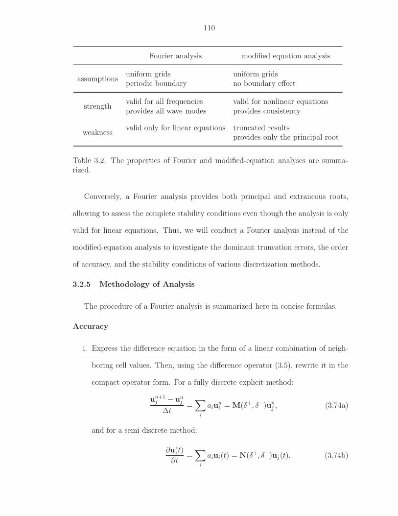
110
Fourier analysis modified equation analysis
assumptionsuniform grids uniform gridsperiodic boundary no boundary effect
strengthvalid for all frequencies valid for nonlinear equationsprovides all wave modes provides consistency
weaknessvalid only for linear equations truncated results
provides only the principal root
Table 3.2: The properties of Fourier and modified-equation analyses are summa-rized.
Conversely, a Fourier analysis provides both principal and extraneous roots,
allowing to assess the complete stability conditions even though the analysis is only
valid for linear equations. Thus, we will conduct a Fourier analysis instead of the
modified-equation analysis to investigate the dominant truncation errors, the order
of accuracy, and the stability conditions of various discretization methods.
3.2.5 Methodology of Analysis
The procedure of a Fourier analysis is summarized here in concise formulas.
Accuracy
1. Express the difference equation in the form of a linear combination of neigh-
boring cell values. Then, using the difference operator (3.5), rewrite it in the
compact operator form. For a fully discrete explicit method:
un+1j − un
j
∆t=∑
i
aiuni = M(δ+, δ−)un
j , (3.74a)
and for a semi-discrete method:
∂u(t)
∂t=∑
i
aiui(t) = N(δ+, δ−)uj(t). (3.74b)
111
2. Once a compact form is obtained, replace difference operators for a Fourier
mode by (3.16). The eigenvalues of a spatial discretization operator are given
by solving the following characteristic equations:
fully discrete : det [M(β) − λ(β)I] = 0, (3.75a)
semi-discrete : det [N(β) − λ(β)I] = 0. (3.75b)
The order of the spatial accuracy can be found by identifying the lowest-order
term of the series expansion of an accurate eigenvalue, given by
λ(β) =∞∑
n=1
bnβn. (3.76)
3. To examine the order of accuracy in both space and time, a fully discrete
method is combined with the forward Euler method, and a semi-discrete
method is incorporated in an RKs method given by (3.11). The amplification
matrices (or factors) are given by
fully discrete : GM(β) = I + ∆tM(β), (3.77a)
semi-discrete : GN(β) = RKs (N(β)) . (3.77b)
When G is a matrix, amplification factors, g(β), are obtained by solving the
following characteristic equation:
det [G(β) − g(β)I ] = 0. (3.78)
Once an amplification factor is obtained, it can be written in the polar form
to decouple the dissipation and dispersion errors:
g = |g|eiφ, (3.79)
112
where
|g(β)| =
∞∑
n=0
b2nβ2n, (3.80a)
φ(β) =
∞∑
n=0
b2n+1β2n+1. (3.80b)
Since the formulas of |g| and φ are lengthly for a higher-order method, they will
be presented only in the form of a power series with respect to the frequency
of a wave.
4. Once a modulus, |g|, and phase angle, φ, are known, the local truncation error
is obtained by the following formula:
LTEmethod = λmethod − λexact
=1
∆tln g − λexact
=1
∆t(ln|g|+ iφ) − λexact
=1
∆t
[ib1β + b2β
2 + ib3β3 − 1
2(b2
2 − 2b4)β4 + . . .
]− λexact. (3.81)
In order to correspond to the result from the modified-equation analysis, wave
frequency, β, is replaced by β = k∆x, thus
LTEmethod =1
ν
[ib1k + b2∆xk2 + ib3∆x2k3 +
(b4 −
1
2b22
)∆x3k4 + . . .
]
− (−irk). (3.82)
Here, we implicitly assume that the grid size, ∆x, is fixed. As long as a
method is consistent with the original PDE, it satisfies b1 ≡ −rν, thus the
above equations is further simplified:
LTEmethod =1
ν
[b2∆xk2 + ib3∆x2k3 +
(b4 −
1
2b2
)∆x3k4 + . . .
]
=∞∑
n=2
cnkn, (3.83)
113
where
c2 =∆x
νb2, c3 = i
∆x2
νb3, and c4 =
∆x3
ν
(b4 −
1
2b2
). (3.84)
The overall order of accuracy can be found by the coefficient of the lowest
order, cn. For instance, if cn = O(∆x, ∆t), then a method is first-order in
space and time.
An alternative way to obtain the coefficient, cn, is directly computing it from
an accurate amplification factor, g(k). Hence, the cn is given by a Taylor
series expansion around k = 0:
cn =1
n!
∂nλ(k)
∂kn
∣∣∣∣k=0
=1
n!∆tg(k = 0)
∂ng(k)
∂kn
∣∣∣∣k=0
. (3.85)
Stability
Ideally, the stability criterion is directly obtained from the modulus of an am-
plification factor, |gmethod|. However, a high-order method tends to have a lengthly
expression for this modulus, and in most of the cases, extracting a stability con-
dition from a modulus is not feasible. The heuristic stability analysis provides a
necessary stability condition, (3.68), yet not sufficient. An alternative way to iden-
tify a stability condition for a high-order method is based on the numerical contour
plot of the modulus, |gmethod(ν, β)|. Using a contour plot, we find the maximum
allowable Courant number, νmax, such that |gmethod(νmax, β)| ≤ 1 for any β ∈ [0, π].
3.3 Difference Operators and Their Properties in 1-D
In this section, a Fourier analysis is employed to uncover the dominant truncation
errors in the low-frequency limit, the order of accuracy, and the stability conditions
of various discretization methods.
114
3.3.1 HR–MOL Method
A semi-discrete high-resolution Godunov method combined with the method-
of-lines (HR–MOL) for the 1-D linear advection equation (3.1a) has the following
form:
∂uj(t)
∂t= − 1
∆x
(fj+1/2(t) − fj−1/2(t)
), (3.86)
where the linear flux, f(u(t)) = ru(t), is evaluated at each cell interface. The
interface flux fj±1/2(t) must be evaluated at various time levels, depending on the
time discretization method (ODE solver) chosen. The interface flux is obtained as
in the q-flux (3.27). For the linear advection equation, it becomes
fj+1/2(t) =r
2
(uj+1/2,L(t)+uj+1/2,R(t)
)−q
2
(uj+1/2,R(t)−uj+1/2,L(t)
), q > 0, (3.87)
where the input values of the flux function are the linearly reconstructed values at
the cell interface j + 1/2:
uj+1/2,L(t) = uj +∆x
2
(∆uj
∆x
), (3.88a)
uj+1/2,R(t) = uj+1 −∆x
2
(∆uj+1
∆x
). (3.88b)
The slopes,∆uj,j+1
∆x, approximate the derivative,
∂u
∂x, and are given by the average
of the differences with the neighboring cells:
∆uj
∆x=
1
2
(uj+1 − uj
∆x+
uj − uj−1
∆x
)=
uj+1 − uj−1
2∆x, (3.89a)
∆uj+1
∆x=
uj+2 − uj
2∆x. (3.89b)
The linear reconstruction from the original piecewise constant values leads an HR–MOL
method to second-order accuracy in space whereas the original Godunov method,
which uses the piecewise constant data, is first-order accurate. Here, we denote the
second-order semi-discrete Godunov method as HR2–MOL.
115
After inserting the cell interface fluxes into the original semi-discrete form (3.86),
and some algebra, the spatial difference operator, NHR2, in the semi-discrete form
of (3.10) is given by
NHR2 = − 1
8∆x
[(q − r)(δ+)2 − 2(q − 2r)δ+ + 2(q + 2r)δ− + (q + r)(δ−)2
],
(3.90a)
or, for a Fourier mode, using (3.16),
NHR2 = − 1
8∆x
[(q − r)e2iβ + 2(3r − 2q)eiβ + 6q − 2(2q + 3r)e−iβ + (q + r)e−2iβ
].
(3.90b)
The identical result can be obtained by setting ν = 0 in the spatial-temporal op-
erator for the Hancock method (3.116), derived further below. To check whether
the method satisfies the shift condition described on page 96, take the upwind flux,
q = r, with the unity Courant number, and multiply by the time step, ∆t, then
∆t NHR2, upwind = − r∆t
4∆x
[δ+ + 3δ− + (δ−)2
]
= −1
4
[δ+ + 3δ− + (δ−)2
]. (3.91)
Since the spatial difference operator contains the forward difference operator, δ+,
no RK methods, which yield polynomials of ∆t NHR2, can produce the exact shift
operator, 1− δ−. Thus, the HR2–MOL method does not satisfy the shift condition.
Accuracy
Taking the low-frequency limit of the spatial difference operator, NHR2, leads to
the asymptotic eigenvalue:
λHR2 = − ir
∆xβ − ir
12∆xβ3 − q
8∆xβ4 + O
(β5). (3.92)
116
The order of accuracy in space is obtained by replacing β by the wave number k,
then
λHR2 − λexact = − ir
12∆x2 k3 − q
8∆x3 k4 + O
(k5); (3.93)
the method appears to be second-order accurate in space.
To examine the overall order of accuracy, the RK2 and RK3 methods (3.11) are
employed for the time integration. The amplification factors, gHR2RK2 and gHR2RK3,
are expressed in the polar form where the modulus and the phase angle of the
HR2–RK2 method are given by
|gHR2RK2| = 1 − rν
8
[qr− (rν)3
]β4 + O
(β6), (3.94a)
φHR2RK2 = −rνβ − rν
12
[1 + 2(rν)2
]β3 + O
(β5), (3.94b)
and for the HR2–RK3 method,
|gHR2RK3| = 1 − rν
8
[q
r+
1
3(rν)3
]β4 + O
(β6), (3.95a)
φHR2RK3 = −rνβ − rν
12β3 + O
(β5). (3.95b)
Following the same procedure, the local truncation errors have the following forms:
LTEHR2RK2 = λHR2RK2 − λexact
=1
∆t(ln|gHR2RK2| + iφHR2RK2) − λexact
= − ir
12
[1 + 2(rν)2
]∆x2 k3 − r
8
[qr− (rν)3
]∆x3k4 + O
(k5)
= − ir
12
(∆x2 + 2r2 ∆t2
)k3 + O
(k4), (3.96a)
LTEHR2RK3 = λHR2RK3 − λexact
= − ir
12∆x2 k3 − r
8
(q
r∆x3 +
1
3r3 ∆t3
)k4 + O
(k5). (3.96b)
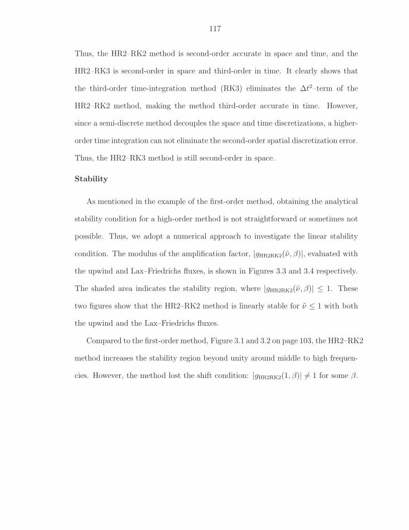
117
Thus, the HR2–RK2 method is second-order accurate in space and time, and the
HR2–RK3 is second-order in space and third-order in time. It clearly shows that
the third-order time-integration method (RK3) eliminates the ∆t2–term of the
HR2–RK2 method, making the method third-order accurate in time. However,
since a semi-discrete method decouples the space and time discretizations, a higher-
order time integration can not eliminate the second-order spatial discretization error.
Thus, the HR2–RK3 method is still second-order in space.
Stability
As mentioned in the example of the first-order method, obtaining the analytical
stability condition for a high-order method is not straightforward or sometimes not
possible. Thus, we adopt a numerical approach to investigate the linear stability
condition. The modulus of the amplification factor, |gHR2RK2(ν, β)|, evaluated with
the upwind and Lax–Friedrichs fluxes, is shown in Figures 3.3 and 3.4 respectively.
The shaded area indicates the stability region, where |gHR2RK2(ν, β)| ≤ 1. These
two figures show that the HR2–RK2 method is linearly stable for ν ≤ 1 with both
the upwind and the Lax–Friedrichs fluxes.
Compared to the first-order method, Figure 3.1 and 3.2 on page 103, the HR2–RK2
method increases the stability region beyond unity around middle to high frequen-
cies. However, the method lost the shift condition: |gHR2RK2(1, β)| 6= 1 for some β.
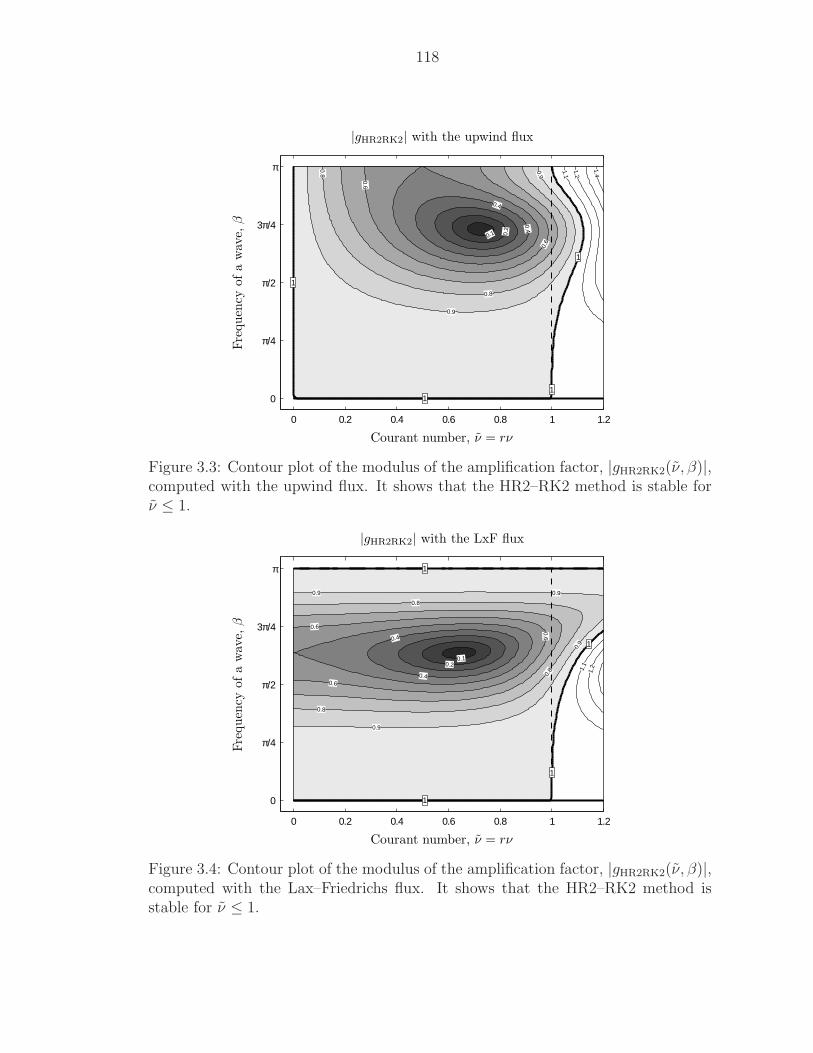
118
0 0.2 0.4 0.6 0.8 1 1.2
0
π/4
π/2
3π/4
π
0.6
0.6
0.8
0.8
0.9
0.9
0.4
0.4
1.1
1.2
0.2
0.1
1.4
1
1
1
1
Courant number, ν = rν
Fre
quen
cyofa
wav
e,β
|gHR2RK2| with the upwind flux
Figure 3.3: Contour plot of the modulus of the amplification factor, |gHR2RK2(ν, β)|,computed with the upwind flux. It shows that the HR2–RK2 method is stable forν ≤ 1.
0 0.2 0.4 0.6 0.8 1 1.2
0
π/4
π/2
3π/4
π
0.6
0.6
0.6
0.8
0.8
0.8
0.9
0.9
0.90.9
0.4
0.4
1.10.2
1.2
0.1
1
1
1
1
Courant number, ν = rν
Fre
quen
cyofa
wav
e,β
|gHR2RK2| with the LxF flux
Figure 3.4: Contour plot of the modulus of the amplification factor, |gHR2RK2(ν, β)|,computed with the Lax–Friedrichs flux. It shows that the HR2–RK2 method isstable for ν ≤ 1.
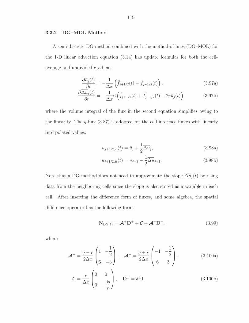
119
3.3.2 DG–MOL Method
A semi-discrete DG method combined with the method-of-lines (DG–MOL) for
the 1-D linear advection equation (3.1a) has update formulas for both the cell-
average and undivided gradient,
∂uj(t)
∂t= − 1
∆x
(fj+1/2(t) − fj−1/2(t)
), (3.97a)
∂∆uj(t)
∂t= − 1
∆x6(fj+1/2(t) + fj−1/2(t) − 2ruj(t)
), (3.97b)
where the volume integral of the flux in the second equation simplifies owing to
the linearity. The q-flux (3.87) is adopted for the cell interface fluxes with linearly
interpolated values:
uj+1/2,L(t) = uj +1
2∆uj , (3.98a)
uj+1/2,R(t) = uj+1 −1
2∆uj+1. (3.98b)
Note that a DG method does not need to approximate the slope ∆uj(t) by using
data from the neighboring cells since the slope is also stored as a variable in each
cell. After inserting the difference form of fluxes, and some algebra, the spatial
difference operator has the following form:
NDG(1) = A+D+ + C + A
−D−, (3.99)
where
A+ =
q − r
2∆x
1 −1
2
6 −3
, A
− =q + r
2∆x
−1 −1
2
6 3
, (3.100a)
C =r
∆x
0 0
0 −6q
r
, D± = δ±I, (3.100b)
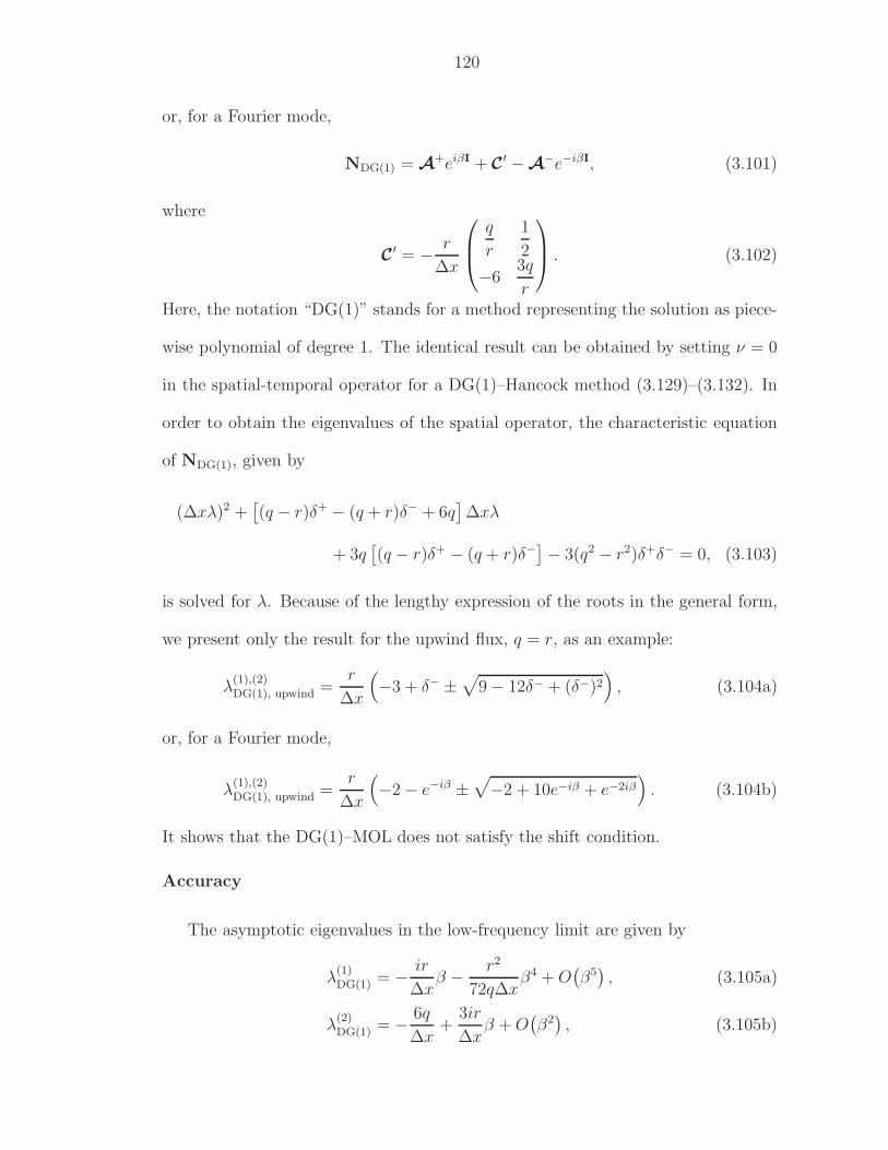
120
or, for a Fourier mode,
NDG(1) = A+eiβI + C
′ − A−e−iβI, (3.101)
where
C′ = − r
∆x
q
r
1
2
−63q
r
. (3.102)
Here, the notation “DG(1)” stands for a method representing the solution as piece-
wise polynomial of degree 1. The identical result can be obtained by setting ν = 0
in the spatial-temporal operator for a DG(1)–Hancock method (3.129)–(3.132). In
order to obtain the eigenvalues of the spatial operator, the characteristic equation
of NDG(1), given by
(∆xλ)2 +[(q − r)δ+ − (q + r)δ− + 6q
]∆xλ
+ 3q[(q − r)δ+ − (q + r)δ−
]− 3(q2 − r2)δ+δ− = 0, (3.103)
is solved for λ. Because of the lengthy expression of the roots in the general form,
we present only the result for the upwind flux, q = r, as an example:
λ(1),(2)DG(1), upwind =
r
∆x
(−3 + δ− ±
√9 − 12δ− + (δ−)2
), (3.104a)
or, for a Fourier mode,
λ(1),(2)DG(1), upwind =
r
∆x
(−2 − e−iβ ±
√−2 + 10e−iβ + e−2iβ
). (3.104b)
It shows that the DG(1)–MOL does not satisfy the shift condition.
Accuracy
The asymptotic eigenvalues in the low-frequency limit are given by
λ(1)DG(1) = − ir
∆xβ − r2
72q∆xβ4 + O
(β5), (3.105a)
λ(2)DG(1) = − 6q
∆x+
3ir
∆xβ + O
(β2), (3.105b)
121
where the former is the principal root and the latter is the extraneous one. Since
a temporal discretization has not been considered yet, all errors appearing here are
attributed solely to the spatial discretization. The order of accuracy in space is
obtained by replacing β by the wave number k, then
λ(1)DG(1) − λexact = − r2
72q∆x3 k4 + O
(k5), (3.106a)
λ(2)DG(1) − λexact = − 6q
∆x+ O(k) , (3.106b)
thus the principal root is third-order accurate in space, and the extraneous root
is zeroth-order. Fortunately, the extraneous root damps quickly since the leading
error, − 6q
∆x, is a large negative real value.
To examine the overall accuracy, time integration methods RK2 and RK3 given
by (3.11) are employed. The amplification factors of the principal root are expressed
in the polar form where the modulus and the phase angle of the DG(1)–RK2 method
are given by
|g(1)DG(1)RK2| = 1 − rν
72
[r
q− 9(rν)3
]β4 + O
(β6), (3.107a)
φ(1)DG(1)RK2 = −rνβ − 1
6(rν)3 + O
(β5), (3.107b)
and for the DG(1)–RK3 method,
|g(2)DG(1)RK3| = 1 − rν
72
[r
q+ 3(rν)3
], (3.108a)
φ(2)DG(1)RK3 = −rνβ + O
(β5). (3.108b)
122
Thus, the local truncation errors become
LTEDG(1)RK2 = λDG(1)RK2 − λexact
=1
∆t
(ln|g(1)
DG(1)RK2| + iφ(1)DG(1)RK2
)λexact
= −ir
6(rν)2∆x2k3 − r
72
(r
q− 9(rν)3
)∆x3k4
= −ir3
6∆t2 k3 − r
72
(r
q∆x3 − 9r3∆t3
)k4 + O
(k5). (3.109a)
LTEDG(1)RK3 = λDG(1)RK3 − λexact
= − r
72
(r
q∆x3 + 3r3 ∆t3
)k4 + O
(k5). (3.109b)
The first equation shows that the temporal discretization RK2 introduces a second-
order error in the DG(1)–RK2 method, hence the DG(1)–RK2 method is third-order
in space, yet second-order in time. Since the RK3 method is third-order accurate,
the DG(1)–RK3 method is third-order in both space and in time.
Stability
The stability domain of the DG(1)–RK2 method was first presented by Cock-
burn and Shu [CS91], and they referred to the stability proof for a simpler case by
Chavent and Cockburn [CC87, CC89]. Here, we present the stability limit by plot-
ting the modulus of the two amplification factors independently. The modulus of the
accurate and inaccurate amplification factors, |g(1),(2)DG(1)RK2|, computed with the up-
wind flux are shown in Figures 3.5(a) and 3.5(b) respectively. The figures show that
the accurate amplification factor possesses a larger stability domain (νmax = 0.468)
than the inaccurate amplification factor (νmax = 1/3). Overall, the stability is con-
strained by the inaccurate amplification factor, so DG(1)–RK2 with the upwind flux
is stable for ν ≤ 1
3.
Counterintuitive results are shown in Figures 3.6(a) and 3.6(b), where the Lax–
123
Friedrichs flux is employed. The contour plots of the modulus show that neither the
accurate nor inaccurate amplification factor is stable for any Courant number, even
when ν = 0. Thus, the DG(1)–RK2 with the Lax–Friedrichs flux is unconditionally
unstable. This was originally found by Rider and Lowrie [RL02]. The same result
is obtained for the DG(1)–RK3 method. This is somewhat surprising since the
Lax–Friedrichs flux adopts the largest possible dissipation coefficient,∆x
∆t, among
all q-fluxes to stabilize the method.
A reason for the destabilizing result produced by this most dissipative flux func-
tion can be found by comparing the dominant numerical dissipation in (3.109) to
that in (3.96). For a DG method, the dissipation parameter q appears in the denomi-
nator, whereas an HR method contains it in the numerator. Thus, for a DG method,
as the numerical dissipation in the flux increases, the method actually becomes less
dissipative, at least for low frequencies. This is completely opposite to the behavior
of an HR method. Hence, the most dissipative flux leads to the least low-frequency
dissipation, resulting in an unconditionally unstable DG method. More specifi-
cally, the instability originates in the extraneous root, λ(2)DG(1). The leading error in
the extraneous root, multiplied by the time step ∆t (this product appears when a
time integration method is applied), evaluated with the upwind and Lax–Friedrichs
fluxes, reads:
Lax–Friedreich : ∆t λ(2),LxFDG(1) = − ∆t
6q
∆x= −6, (3.110a)
upwind : ∆t λ(2),upwindDG(1) = − ∆t
6r
∆x= −6ν. (3.110b)
Assume, for instance, that the RK2 method is used for time integration, then the
above eigenvalues should satisfy a necessary condition, ℜ[∆t λ] ∈ [−2, 0], for stabil-
ity in the low-frequency limit. The second equation, for the upwind flux, satisfies
124
this stability condition as long as ν ≤ 1
3. Conversely, the first equation never sat-
isfies the stability condition, no matter how small the time step is; thus, DG(1)
together with the Lax–Friedrichs flux is unconditionally unstable.
To remedy the instability of the Lax–Friedrichs flux, Rider and Lowrie propose
the following modified Lax–Friedrichs flux [RL02]:
fmLxFj+1/2(uL, uR) =
r
2(uL + uR) − z
2
∆x
∆x(uR − uL), (3.111)
where z =1
3for DG(1), and z =
1
5for DG(2). These constants are chosen such that
the maximum stable Courant number is the same as for the DG method combined
with the upwind flux. The motivation of the choice of constant becomes clear when
the leading error is again considered:
modified Lax–Friedrichs: ∆tλ(2),mLxFDG(1) = −∆t
6 qmLxF
∆x
= −6z, (3.112)
thus as long as z ≤ 1
3, the leading error satisfies the stability condition, ℜ[∆t λ] ∈
[−2, 0]. Since the condition is merely necessary and not sufficient, the full stability
domains based on the modified Lax–Friedrichs flux are obtained numerically and
shown in Figures 3.7(a) and 3.7(b). For this flux function, both accurate and
inaccurate eigenmodes possess the same stability limit, ν ≤ 0.424. This is less
restrictive than the DG(1)–RK2 with the upwind flux; however, it can be observed
that the modified Lax–Friedrichs flux is more dissipative than the upwind flux,
especially for high frequency modes.
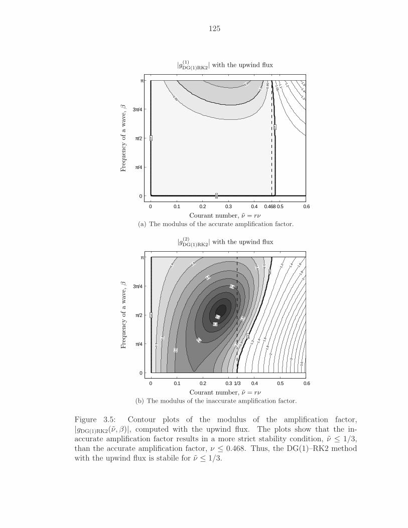
125
0 0.1 0.2 0.3 0.4 0.468 0.5 0.6
0
π/4
π/2
3π/4
π0.8
0.9
0.95
0.95 1.05
1.1
1.2
1.31.4
1.5
1
1
1
Courant number, ν = rν
Fre
quen
cyofa
wav
e,β
|g(1)DG(1)RK2| with the upwind flux
(a) The modulus of the accurate amplification factor.
0 0.1 0.2 0.3 1/3 0.4 0.5 0.6
0
π/4
π/2
3π/4
π
0.6
0.6
0.6
0.8
0.8
0.9
0.9
1.2
1.2
1.4
1.4
1.6
1.6
1.8
1.8
2
2
0.8
0.8
0.4
0.4
0.9
0.9
3
0.2
3.6
0.1
1
1
1
Courant number, ν = rν
Fre
quen
cyofa
wav
e,β
|g(2)DG(1)RK2| with the upwind flux
(b) The modulus of the inaccurate amplification factor.
Figure 3.5: Contour plots of the modulus of the amplification factor,|gDG(1)RK2(ν, β)|, computed with the upwind flux. The plots show that the in-accurate amplification factor results in a more strict stability condition, ν ≤ 1/3,than the accurate amplification factor, ν ≤ 0.468. Thus, the DG(1)–RK2 methodwith the upwind flux is stabile for ν ≤ 1/3.
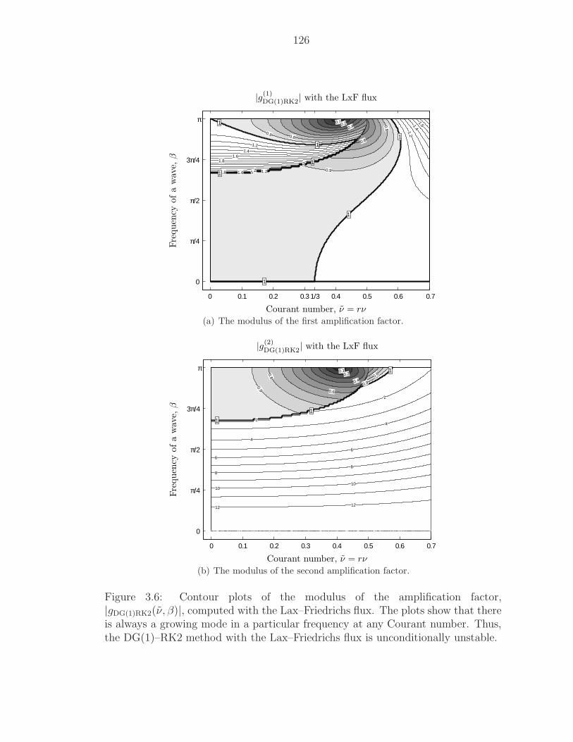
126
0 0.1 0.2 0.3 1/3 0.4 0.5 0.6 0.7
0
π/4
π/2
3π/4
π 0.10.2
0.4
0.60.8
0.8
0.9
0.9
1.2
1.2
1.4
1.4
1.6
1.6
1.8
1.8
1.2
2
1.41.6
2
1
1
1
1
1
1
1
Courant number, ν = rν
Fre
quen
cyofa
wav
e,β
|g(1)DG(1)RK2| with the LxF flux
(a) The modulus of the first amplification factor.
0 0.1 0.2 0.3 0.4 0.5 0.6 0.7
0
π/4
π/2
3π/4
π 0.10.2
0.4
0.6
0.8 0.8
0.9
0.9
2
2
4
4
6
6
88
1010
12 12
1
1
1
Courant number, ν = rν
Fre
quen
cyofa
wav
e,β
|g(2)DG(1)RK2| with the LxF flux
(b) The modulus of the second amplification factor.
Figure 3.6: Contour plots of the modulus of the amplification factor,|gDG(1)RK2(ν, β)|, computed with the Lax–Friedrichs flux. The plots show that thereis always a growing mode in a particular frequency at any Courant number. Thus,the DG(1)–RK2 method with the Lax–Friedrichs flux is unconditionally unstable.
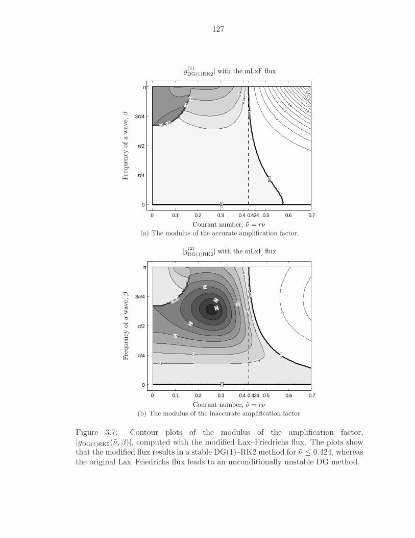
127
0 0.1 0.2 0.3 0.4 0.424 0.5 0.6 0.7
0
π/4
π/2
3π/4
π
0.6
0.8
0.9
0.9
0.95
0.95
1.2
1.41.6
1.8
2
2.2
2.4
1
1
1
Courant number, ν = rν
Fre
quen
cyofa
wav
e,β
|g(1)DG(1)RK2| with the mLxF flux
(a) The modulus of the accurate amplification factor.
0 0.1 0.2 0.3 0.4 0.424 0.5 0.6 0.7
0
π/4
π/2
3π/4
π
0.6
0.6
0.6
0.8
0.8
0.90.9
0.9
2
0.4
0.4
0.80.90.2
0.1
1
1
1
Courant number, ν = rν
Fre
quen
cyofa
wav
e,β
|g(2)DG(1)RK2| with the mLxF flux
(b) The modulus of the inaccurate amplification factor.
Figure 3.7: Contour plots of the modulus of the amplification factor,|gDG(1)RK2(ν, β)|, computed with the modified Lax–Friedrichs flux. The plots showthat the modified flux results in a stable DG(1)–RK2 method for ν ≤ 0.424, whereasthe original Lax–Friedrichs flux leads to an unconditionally unstable DG method.
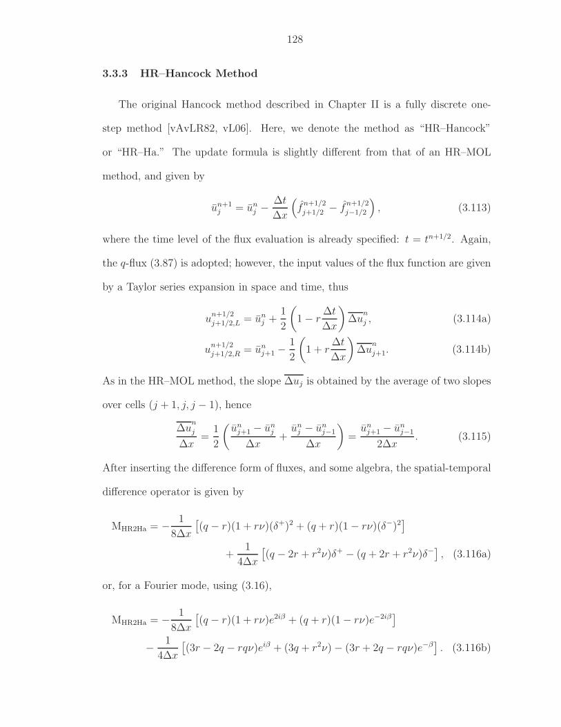
128
3.3.3 HR–Hancock Method
The original Hancock method described in Chapter II is a fully discrete one-
step method [vAvLR82, vL06]. Here, we denote the method as “HR–Hancock”
or “HR–Ha.” The update formula is slightly different from that of an HR–MOL
method, and given by
un+1j = un
j − ∆t
∆x
(f
n+1/2j+1/2 − f
n+1/2j−1/2
), (3.113)
where the time level of the flux evaluation is already specified: t = tn+1/2. Again,
the q-flux (3.87) is adopted; however, the input values of the flux function are given
by a Taylor series expansion in space and time, thus
un+1/2j+1/2,L = un
j +1
2
(1 − r
∆t
∆x
)∆u
n
j , (3.114a)
un+1/2j+1/2,R = un
j+1 −1
2
(1 + r
∆t
∆x
)∆u
n
j+1. (3.114b)
As in the HR–MOL method, the slope ∆uj is obtained by the average of two slopes
over cells (j + 1, j, j − 1), hence
∆un
j
∆x=
1
2
(un
j+1 − unj
∆x+
unj − un
j−1
∆x
)=
unj+1 − un
j−1
2∆x. (3.115)
After inserting the difference form of fluxes, and some algebra, the spatial-temporal
difference operator is given by
MHR2Ha = − 1
8∆x
[(q − r)(1 + rν)(δ+)2 + (q + r)(1 − rν)(δ−)2
]
+1
4∆x
[(q − 2r + r2ν)δ+ − (q + 2r + r2ν)δ−
], (3.116a)
or, for a Fourier mode, using (3.16),
MHR2Ha = − 1
8∆x
[(q − r)(1 + rν)e2iβ + (q + r)(1 − rν)e−2iβ
]
− 1
4∆x
[(3r − 2q − rqν)eiβ + (3q + r2ν) − (3r + 2q − rqν)e−β
]. (3.116b)
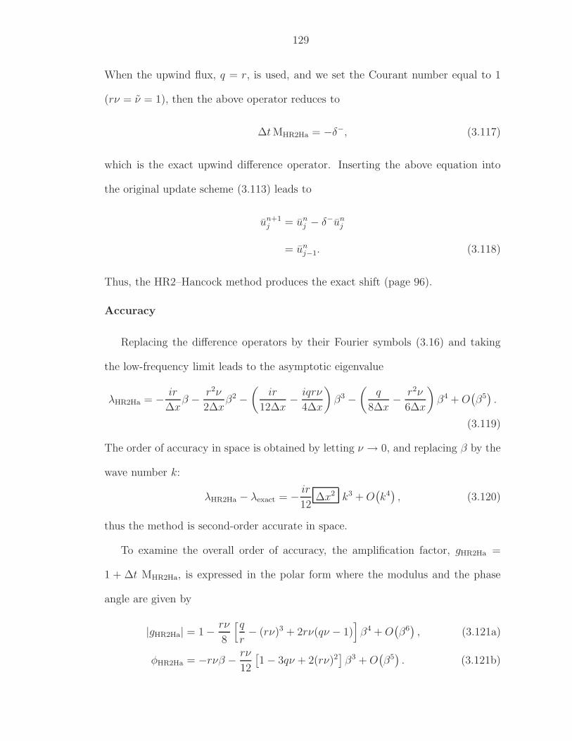
129
When the upwind flux, q = r, is used, and we set the Courant number equal to 1
(rν = ν = 1), then the above operator reduces to
∆t MHR2Ha = −δ−, (3.117)
which is the exact upwind difference operator. Inserting the above equation into
the original update scheme (3.113) leads to
un+1j = un
j − δ−unj
= unj−1. (3.118)
Thus, the HR2–Hancock method produces the exact shift (page 96).
Accuracy
Replacing the difference operators by their Fourier symbols (3.16) and taking
the low-frequency limit leads to the asymptotic eigenvalue
λHR2Ha = − ir
∆xβ − r2ν
2∆xβ2 −
(ir
12∆x− iqrν
4∆x
)β3 −
(q
8∆x− r2ν
6∆x
)β4 + O
(β5).
(3.119)
The order of accuracy in space is obtained by letting ν → 0, and replacing β by the
wave number k:
λHR2Ha − λexact = − ir
12∆x2 k3 + O
(k4), (3.120)
thus the method is second-order accurate in space.
To examine the overall order of accuracy, the amplification factor, gHR2Ha =
1 + ∆t MHR2Ha, is expressed in the polar form where the modulus and the phase
angle are given by
|gHR2Ha| = 1 − rν
8
[qr− (rν)3 + 2rν(qν − 1)
]β4 + O
(β6), (3.121a)
φHR2Ha = −rνβ − rν
12
[1 − 3qν + 2(rν)2
]β3 + O
(β5). (3.121b)
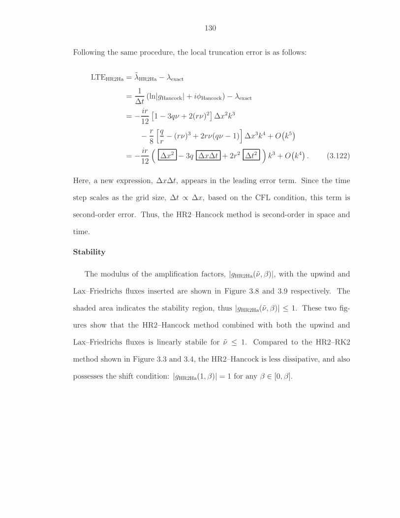
130
Following the same procedure, the local truncation error is as follows:
LTEHR2Ha = λHR2Ha − λexact
=1
∆t(ln|gHancock| + iφHancock) − λexact
= − ir
12
[1 − 3qν + 2(rν)2
]∆x2k3
− r
8
[qr− (rν)3 + 2rν(qν − 1)
]∆x3k4 + O
(k5)
= − ir
12
(∆x2 − 3q ∆x∆t + 2r2 ∆t2
)k3 + O
(k4). (3.122)
Here, a new expression, ∆x∆t, appears in the leading error term. Since the time
step scales as the grid size, ∆t ∝ ∆x, based on the CFL condition, this term is
second-order error. Thus, the HR2–Hancock method is second-order in space and
time.
Stability
The modulus of the amplification factors, |gHR2Ha(ν, β)|, with the upwind and
Lax–Friedrichs fluxes inserted are shown in Figure 3.8 and 3.9 respectively. The
shaded area indicates the stability region, thus |gHR2Ha(ν, β)| ≤ 1. These two fig-
ures show that the HR2–Hancock method combined with both the upwind and
Lax–Friedrichs fluxes is linearly stabile for ν ≤ 1. Compared to the HR2–RK2
method shown in Figure 3.3 and 3.4, the HR2–Hancock is less dissipative, and also
possesses the shift condition: |gHR2Ha(1, β)| = 1 for any β ∈ [0, β].
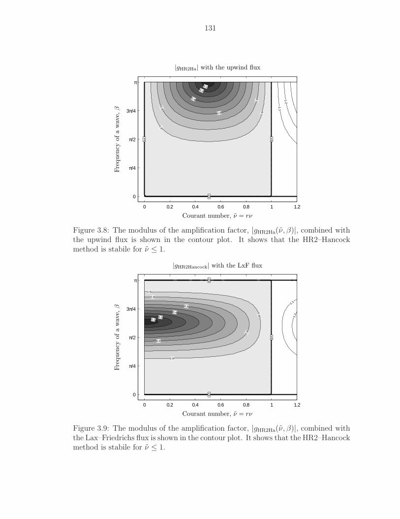
131
0 0.2 0.4 0.6 0.8 1 1.2
0
π/4
π/2
3π/4
π0.1
0.2
0.4
0.6
0.8
0.8
0.9
0.9
1.1
1.2
1
1
1
Courant number, ν = rν
Fre
quen
cyofa
wav
e,β
|gHR2Ha| with the upwind flux
Figure 3.8: The modulus of the amplification factor, |gHR2Ha(ν, β)|, combined withthe upwind flux is shown in the contour plot. It shows that the HR2–Hancockmethod is stabile for ν ≤ 1.
0 0.2 0.4 0.6 0.8 1 1.2
0
π/4
π/2
3π/4
π
0.10.2
0.4
0.6
0.6
0.8
0.8
0.9
0.9
0.9
1.1
1.2
1
1
1
Courant number, ν = rν
Fre
quen
cyofa
wav
e,β
|gHR2Hancock| with the LxF flux
Figure 3.9: The modulus of the amplification factor, |gHR2Ha(ν, β)|, combined withthe Lax–Friedrichs flux is shown in the contour plot. It shows that the HR2–Hancockmethod is stabile for ν ≤ 1.
132
3.3.4 DG–Hancock Method
The DG–Hancock method described in Chapter II is also fully discrete, and
introduces two variables for a scalar equation, yielding a 2×2 amplification matrix.
The update formulas for cell-average and undivided gradient have the following
form:
un+1j = un
j − ∆t
∆x
(f
n+1/2j+1/2 − f
n+1/2j−1/2
), (3.123a)
∆un+1
j = ∆un
j − ∆t
∆x6(f
n+1/2j+1/2 + f
n+1/2j−1/2 − 2ruj
), (3.123b)
where the interface fluxes are evaluated at the time level, tn+1/2, by the q-flux (3.87).
The input values for the flux function at the time level tn+k/2 are given by
un+k/2j+1/2,L = un
j +1
2
(1 − r
k∆t
∆x
)∆u
n
j , (3.124a)
un+k/2j+1/2,R = un
j+1 −1
2
(1 + r
k∆t
∆x
)∆u
n
j+1. (3.124b)
The volume integral of the flux over the domain [xj−1/2, xj+1/2]× [tn, tn+1] simplifies
owing to the linear flux. Hence, the spatial integration is done exactly, and a quadra-
ture is only required in time. Two techniques are employed: 3-point Gauss–Lobatto
and 2-point Gauss–Radau quadratures. These quadratures, with their necessary
intermediate update equation, are as follows:
3-point Gauss–Lobatto
uj,GL =1
6(un
j + 4un+1/2j + un+1
j ), (3.125)
where
un+1/2j = un
j − ∆t
2
1
∆x
(f
n+1/4j+1/2 − f
n+1/4j−1/2
), (3.126)
2-point Gauss–Radau
uj,GR =1
4(3u
n+1/3j + un+1
j ), (3.127)
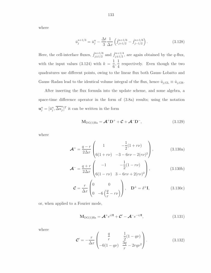
133
where
un+1/3j = un
j − ∆t
3
1
∆x
(f
n+1/6j+1/2 − f
n+1/6j−1/2
). (3.128)
Here, the cell-interface fluxes, fn+1/6j±1/2 and f
n+1/4j±1/2 , are again obtained by the q-flux,
with the input values (3.124) with k =1
6,1
4respectively. Even though the two
quadratures use different points, owing to the linear flux both Gauss–Lobatto and
Gauss–Radau lead to the identical volume integral of the flux, hence uj,GL ≡ uj,GR.
After inserting the flux formula into the update scheme, and some algebra, a
space-time difference operator in the form of (3.8a) results; using the notation
unj = [un
j , ∆un
j ]T it can be written in the form
MDG(1)Ha = A+D+ + C + A
−D−, (3.129)
where
A+ =
q − r
2∆x
1 −1
2(1 + rν)
6(1 + rν) −3 − 6rν − 2(rν)2
, (3.130a)
A− =
q + r
2∆x
−1 −1
2(1 − rν)
6(1 − rν) 3 − 6rν + 2(rν)2
, (3.130b)
C =r
∆x
0 0
0 −6(q
r− rν
)
, D± = δ±I, (3.130c)
or, when applied to a Fourier mode,
MDG(1)Ha = A+eiβI + C
′ − A−e−iβI, (3.131)
where
C′ = − r
∆x
q
r
1
2(1 − qν)
−6(1 − qν)3q
r− 2rqν2
. (3.132)
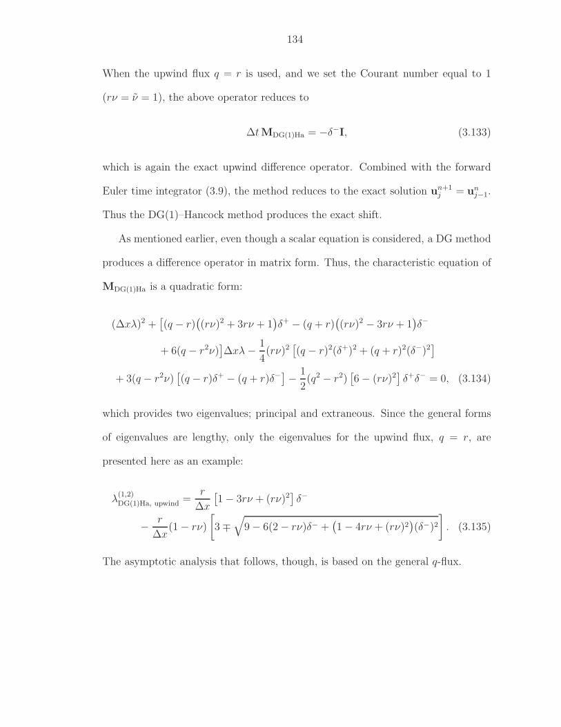
134
When the upwind flux q = r is used, and we set the Courant number equal to 1
(rν = ν = 1), the above operator reduces to
∆tMDG(1)Ha = −δ−I, (3.133)
which is again the exact upwind difference operator. Combined with the forward
Euler time integrator (3.9), the method reduces to the exact solution un+1j = un
j−1.
Thus the DG(1)–Hancock method produces the exact shift.
As mentioned earlier, even though a scalar equation is considered, a DG method
produces a difference operator in matrix form. Thus, the characteristic equation of
MDG(1)Ha is a quadratic form:
(∆xλ)2 +[(q − r)
((rν)2 + 3rν + 1
)δ+ − (q + r)
((rν)2 − 3rν + 1
)δ−
+ 6(q − r2ν)]∆xλ − 1
4(rν)2
[(q − r)2(δ+)2 + (q + r)2(δ−)2
]
+ 3(q − r2ν)[(q − r)δ+ − (q + r)δ−
]− 1
2(q2 − r2)
[6 − (rν)2
]δ+δ− = 0, (3.134)
which provides two eigenvalues; principal and extraneous. Since the general forms
of eigenvalues are lengthy, only the eigenvalues for the upwind flux, q = r, are
presented here as an example:
λ(1,2)DG(1)Ha, upwind =
r
∆x
[1 − 3rν + (rν)2
]δ−
− r
∆x(1 − rν)
[3 ∓
√9 − 6(2 − rν)δ− +
(1 − 4rν + (rν)2
)(δ−)2
]. (3.135)
The asymptotic analysis that follows, though, is based on the general q-flux.
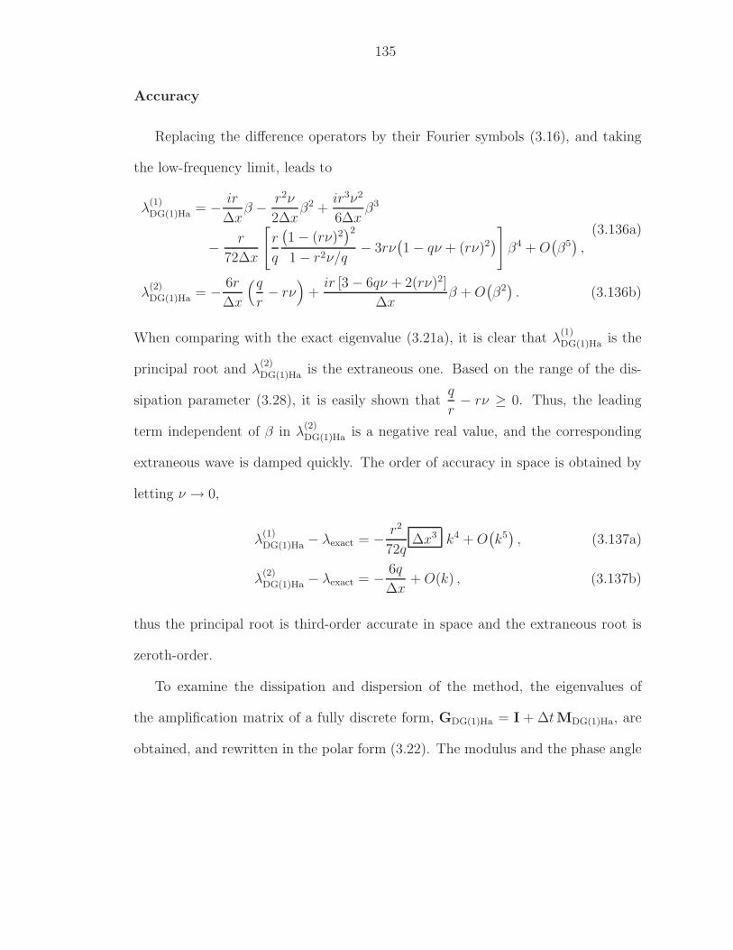
135
Accuracy
Replacing the difference operators by their Fourier symbols (3.16), and taking
the low-frequency limit, leads to
λ(1)DG(1)Ha = − ir
∆xβ − r2ν
2∆xβ2 +
ir3ν2
6∆xβ3
− r
72∆x
[r
q
(1 − (rν)2
)2
1 − r2ν/q− 3rν
(1 − qν + (rν)2
)]
β4 + O(β5),
(3.136a)
λ(2)DG(1)Ha = − 6r
∆x
(q
r− rν
)+
ir [3 − 6qν + 2(rν)2]
∆xβ + O
(β2). (3.136b)
When comparing with the exact eigenvalue (3.21a), it is clear that λ(1)DG(1)Ha is the
principal root and λ(2)DG(1)Ha is the extraneous one. Based on the range of the dis-
sipation parameter (3.28), it is easily shown thatq
r− rν ≥ 0. Thus, the leading
term independent of β in λ(2)DG(1)Ha is a negative real value, and the corresponding
extraneous wave is damped quickly. The order of accuracy in space is obtained by
letting ν → 0,
λ(1)DG(1)Ha − λexact = − r2
72q∆x3 k4 + O
(k5), (3.137a)
λ(2)DG(1)Ha − λexact = − 6q
∆x+ O(k) , (3.137b)
thus the principal root is third-order accurate in space and the extraneous root is
zeroth-order.
To examine the dissipation and dispersion of the method, the eigenvalues of
the amplification matrix of a fully discrete form, GDG(1)Ha = I + ∆tMDG(1)Ha, are
obtained, and rewritten in the polar form (3.22). The modulus and the phase angle
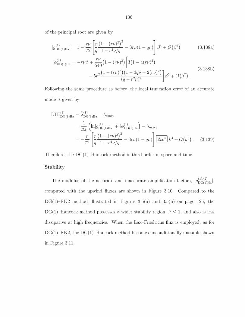
136
of the principal root are given by
|g(1)DG(1)Ha| = 1 − rν
72
[r
q
(1 − (rν)2
)2
1 − r2ν/q− 3rν(1 − qν)
]β4 + O
(β6), (3.138a)
φ(1)DG(1)Ha = −rνβ +
rν
540
(1 − (rν)2
)[3(1 − 4(rν)2
)
− 5r2
(1 − (rν)2
)(1 − 3qν + 2(rν)2
)
(q − r2ν)2
]β5 + O
(β7).
(3.138b)
Following the same procedure as before, the local truncation error of an accurate
mode is given by
LTE(1)DG(1)Ha = λ
(1)DG(1)Ha − λexact
=1
∆t
(ln|g(1)
DG(1)Ha| + iφ(1)DG(1)Ha
)− λexact
= − r
72
[r
q
(1 − (rν)2
)2
1 − r2ν/q− 3rν(1 − qν)
]∆x3 k4 + O
(k5). (3.139)
Therefore, the DG(1)–Hancock method is third-order in space and time.
Stability
The modulus of the accurate and inaccurate amplification factors, |g(1),(2)DG(1)Ha|,
computed with the upwind fluxes are shown in Figure 3.10. Compared to the
DG(1)–RK2 method illustrated in Figures 3.5(a) and 3.5(b) on page 125, the
DG(1)–Hancock method possesses a wider stability region, ν ≤ 1, and also is less
dissipative at high frequencies. When the Lax–Friedrichs flux is employed, as for
DG(1)–RK2, the DG(1)–Hancock method becomes unconditionally unstable shown
in Figure 3.11.
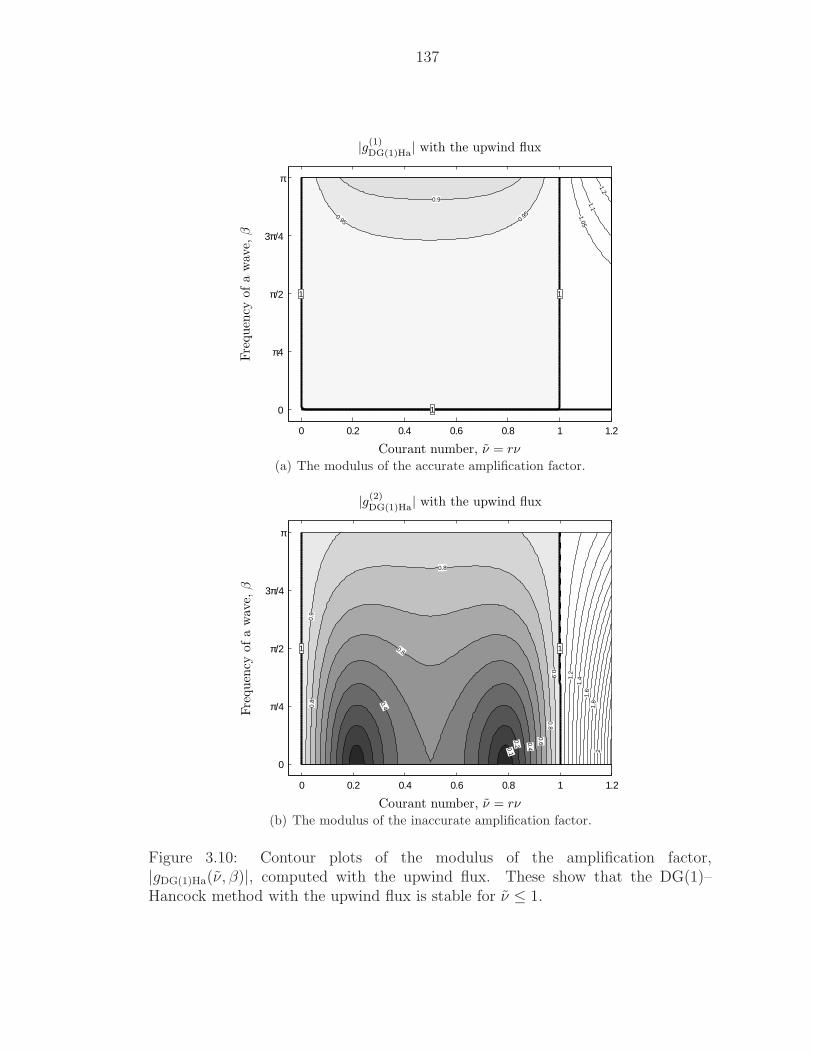
137
0 0.2 0.4 0.6 0.8 1 1.2
0
π4
π/2
3π/4
π
0.9
0.95 0.95 1.05
1.1
1.2
1
1
1
Courant number, ν = rν
Fre
quen
cyofa
wav
e,β
|g(1)DG(1)Ha| with the upwind flux
(a) The modulus of the accurate amplification factor.
0 0.2 0.4 0.6 0.8 1 1.2
0
π/4
π/2
3π/4
π
0.10.2 0.4
0.4
0.6
0.6
0.8
0.8
0.8
0.9
1.2
1.4
1.6
0.9
1.8
2
11
Courant number, ν = rν
Fre
quen
cyofa
wav
e,β
|g(2)DG(1)Ha| with the upwind flux
(b) The modulus of the inaccurate amplification factor.
Figure 3.10: Contour plots of the modulus of the amplification factor,|gDG(1)Ha(ν, β)|, computed with the upwind flux. These show that the DG(1)–Hancock method with the upwind flux is stable for ν ≤ 1.
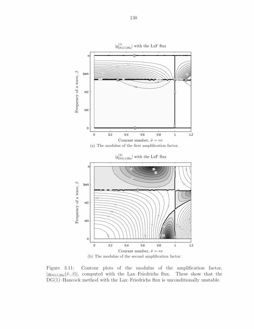
138
0 0.2 0.4 0.6 0.8 1 1.2
0
π/4
π/2
3π/4
π
0.8
0.90.920.960.98
1.1
1.11.1
1.2
1.21.2 0.98
0.98
1.6
1.6 0.96
0.96
11
1
1
1
1
1
Courant number, ν = rν
Fre
quen
cyofa
wav
e,β
|g(1)DG(1)Ha| with the LxF flux
(a) The modulus of the first amplification factor.
0 0.2 0.4 0.6 0.8 1 1.2
0
π/4
π/2
3π/4
π0.2
0.4
0.6
0.6
0.8
0.9
0.9
0.9
1.2
1.2
1.6
1.6
2
2
2.6
2.6
3
3.6
4
1.2
1.6
1.2
2
4.8
2.6
1.6
31
1
11
Courant number, ν = rν
Fre
quen
cyofa
wav
e,β
|g(2)DG(1)Ha| with the LxF flux
(b) The modulus of the second amplification factor.
Figure 3.11: Contour plots of the modulus of the amplification factor,|gDG(1)Ha(ν, β)|, computed with the Lax–Friedrichs flux. These show that theDG(1)–Hancock method with the Lax–Friedrichs flux is unconditionally unstable.
139
3.3.5 Miscellaneous Methods (SV–MOL, DG–ADER)
Even though our main focus in this section is the analysis and comparison
of the DG–Hancock method to the HR/DG–MOL methods, we also present re-
sults for two newly developed high-order methods: the spectral finite volume (SV)
method [Wan02] and the arbitrarily high-order schemes using derivatives (DG–ADER
method) [DM06].
SV–MOL Method
The spectral finite volume method subdivides the spectral volume (SV) into a
few control volumes (CV). The cell-averaged state variables are defined at each CV
inside an SV. For instance, the state variable of the SV over x ∈ [xj−1/2, xj+1/2] is
defined as uj = [uj,1 uj,2] for the second-order method. One of the advantages of
an SV method is that the method does not require the volume integral of a flux
over the SV, whereas a DG method typically employs a quadrature to compute the
volume integral of a flux. Thus, an SV method is computationally less expensive
than a DG method. Furthermore, in general, an SV method has a less restrictive
stability limit than a DG method. However, a DG method tends to provide more
accurate (less dissipative) results than an SV method. A detailed comparison of an
SV to a DG method can be found in [SW04, ZS05].
Here, we consider the second-order SV method (SV2) [Wan02, p. 224]. The
semi-discrete form of the method is given by
∂uj,1(t)
∂t= − 1
∆x/2
(fj+1/2(t) − fj(t)
), (3.140a)
∂uj,2(t)
∂t= − 1
∆x/2
(fj(t) − fj−1/2(t)
), (3.140b)
where the interface fluxes across the SV boundaries, fj±1/2(t), are obtained by the
140
q-flux (3.87) with the following input values:
uj+1/2,L(t) = −1
2uj,1(t) +
3
2uj,2(t), (3.141a)
uj+1/2,R(t) =3
2uj+1,1(t) −
1
2uj+1,2(t). (3.141b)
Since the state variable is continuous across the interior CV boundary at xj , the
flux, fj(t), is obtained analytically such that
fj(u(t)) = fj
(1
2
(uj,1(t) + uj,2(t)
))
=r
2[uj,1(t) + uj,2(t)] . (3.142)
After inserting the flux formula into the update scheme, and some algebra, the
spatial difference operator becomes the following compact form:
NSV2 = A+D+ + C + A
−D−, (3.143)
where
A+ =
q − r
2∆x
0 0
3 −1
, A
− =q + r
2∆x
1 −3
0 0
, (3.144a)
C =2q
∆x
−1 1
1 −1
, D± = δ±I, (3.144b)
or, for a Fourier mode,
NSV2 = A+eiβI + C
′ − A−e−iβI, (3.145)
where
C′ =
1
2∆x
−(3q − r) q − 3r
q + 3r −(3q + r)
. (3.146)
141
Accuracy The eigenvalues of the spatial operator, NSV2, in the low-frequency
limit are as follows:
λ(1)SV2 = − ir
∆xβ +
ir
24∆xβ3 − r2
32q∆xβ4 + O
(β5), (3.147a)
λ(2)SV2 = − 4q
∆x+
2ir
∆xβ + O
(β2). (3.147b)
Similar to a DG discretization, the leading term of the extraneous root has a negative
real value. Thus, the spurious mode is damped quickly. The order of accuracy in
space is obtained by replacing β by the wave number k:
λ(1)SV2 − λexact =
ir
24∆x2 k3 + O
(k4), (3.148a)
λ(2)SV2 − λexact = − 4q
∆x+ O(k) . (3.148b)
Hence, the SV discretization containing two CVs (SV2) is second-order in space.
The overall accuracy can be obtained by combining it with an ODE solver. Here,
the second-order Runge–Kutta (RK2) method is adopted for the time integration.
Following the same procedure as in the previous analysis, the local truncation error
of the SV2–RK2 method is given by
LTESV2RK2 =ir
24
[1 − 4(rν)2
]∆x2k3 − r
32
[r
q− 4(rν)3
]∆x3k4
=ir
24
(∆x2 − 4r2 ∆t2
)k3 − r
32
[r
q− 4(rν)3
]∆x3k4. (3.149)
The above equation shows that the SV2–RK2 method is second-order in space and
time. In contrast to the DG(1)–RK2 method, a higher-order time discretization,
e.g., SV2–RK3, does not increase the overall accuracy since the spatial discretiza-
tion error is still second-order. This is clearly shown by comparing the eigenval-
ues (3.148a) to (3.106a) on page 121.
142
Stability The modulus of the amplification factor, |gSV2RK2(ν, β)|, computed
with the upwind flux is shown in Figure 3.12. Interestingly, the dissipation prop-
erty of the SV2–RK2 method is qualitatively similar to that of the DG(1)–RK2
method shown in Figures 3.5(a) and 3.5(b) on page 125. Both methods are second-
order accurate in space and time, however the stability domains are different: the
SV2–RK2 method has a wider stability domain ν ≤ 1
2, whereas DG(1)–RK2 has
ν ≤ 1
3. This wider stability domain together with the volume-integral free flux
makes the SV2–RK2 method less computationally expensive than the DG(1)–RK2
method. However, the SV2–RK2 tends to be more dissipative than the DG(1)–RK2.
For instance, at low frequencies, the dominant dissipation of the SV2–RK2 is twice
as large as the DG(1)–RK2 method. More detailed comparisons are followed at the
end of the section.
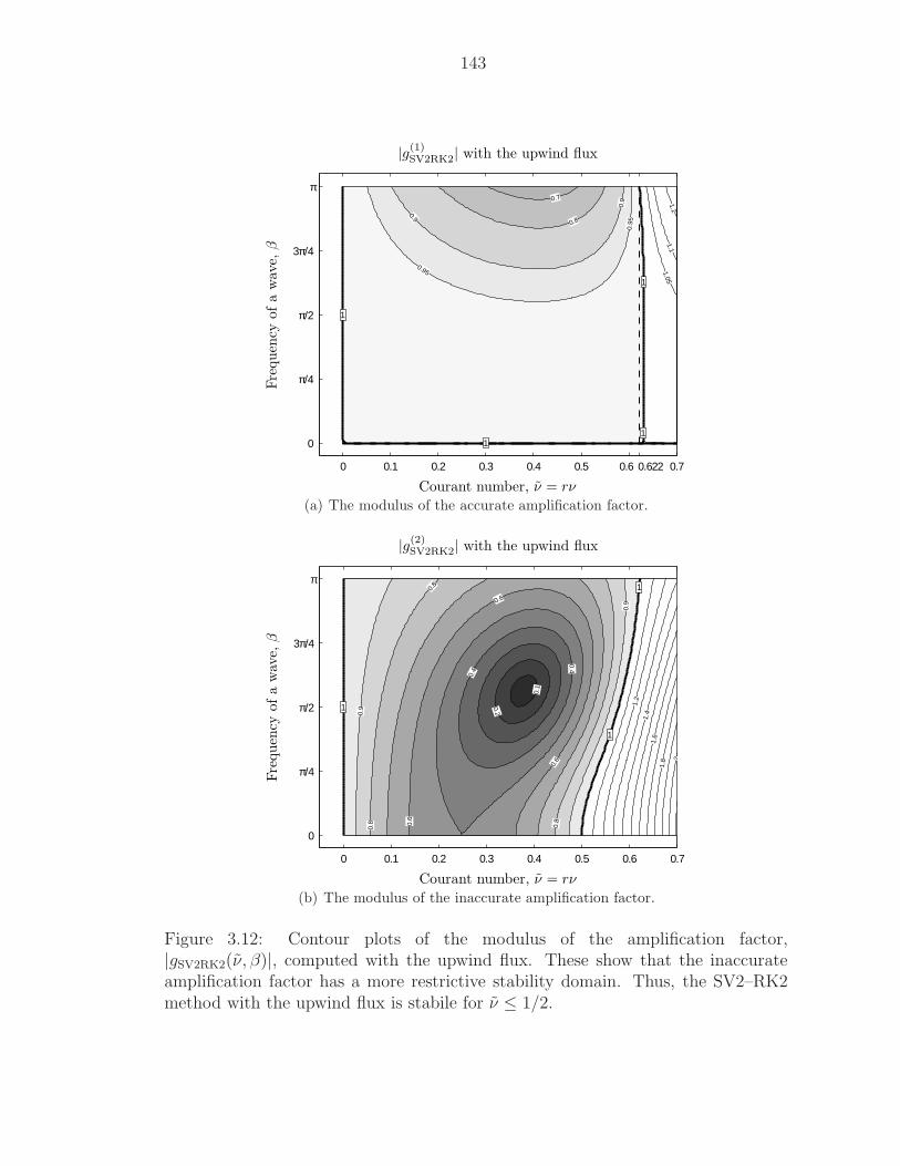
143
0 0.1 0.2 0.3 0.4 0.5 0.6 0.622 0.7
0
π/4
π/2
3π/4
π0.7
0.8
0.9
0.9
0.95
0.95
1.051.1
1.2
1
1
1
1
Courant number, ν = rν
Fre
quen
cyofa
wav
e,β
|g(1)SV2RK2| with the upwind flux
(a) The modulus of the accurate amplification factor.
0 0.1 0.2 0.3 0.4 0.5 0.6 0.7
0
π/4
π/2
3π/4
π
0.6
0.6
0.6
0.8
0.9
0.4
0.4
1.2
0.8
0.8
1.40.
9
1.6
0.2
1.8
0.1
2
1
1
1
Courant number, ν = rν
Fre
quen
cyofa
wav
e,β
|g(2)SV2RK2| with the upwind flux
(b) The modulus of the inaccurate amplification factor.
Figure 3.12: Contour plots of the modulus of the amplification factor,|gSV2RK2(ν, β)|, computed with the upwind flux. These show that the inaccurateamplification factor has a more restrictive stability domain. Thus, the SV2–RK2method with the upwind flux is stabile for ν ≤ 1/2.
144
DG–ADER Method
A DG–ADER method is a fully discrete method, utilizing the Cauchy–Kovalevskaya
procedure to replace the temporal derivatives by the spatial derivatives [DM05].
Even though a DG–ADER method can be extended to an arbitrary high-order of
accuracy, we only analyze the second method, DG(1)–ADER, here. The resulting
method is similar to the DG(1)–Hancock method except for the evaluation of the
volume integral of the flux. For a linear flux, the flux integral in time is approxi-
mated by the flux at the intermediate state, n + 1/2, thus
1
∆t
∫
T n
f(uj)dt ≃ f(un+1/2j ), (3.150)
where the predicted value, un+1/2j , is given by
un+1/2j = un
j − ∆t
2fx(u)
= unj − r∆t
2
∆un
j
∆x. (3.151)
Note that compared to the DG(1)–Hancock method, the volume integral of the
DG(1)–ADER method does not require a Riemann solver; the wave interactions
across the cell interfaces are neglected in the volume integral. Here, we omit
the derivation of the method; the interested reader is referred to the original pa-
pers [DM06, DM05]. The spatial difference operator of the DG(1)–ADER method
together with the q–flux (3.87) has the following form:
MDG(1)ADER = A+D+ + C + A
−D−, (3.152)
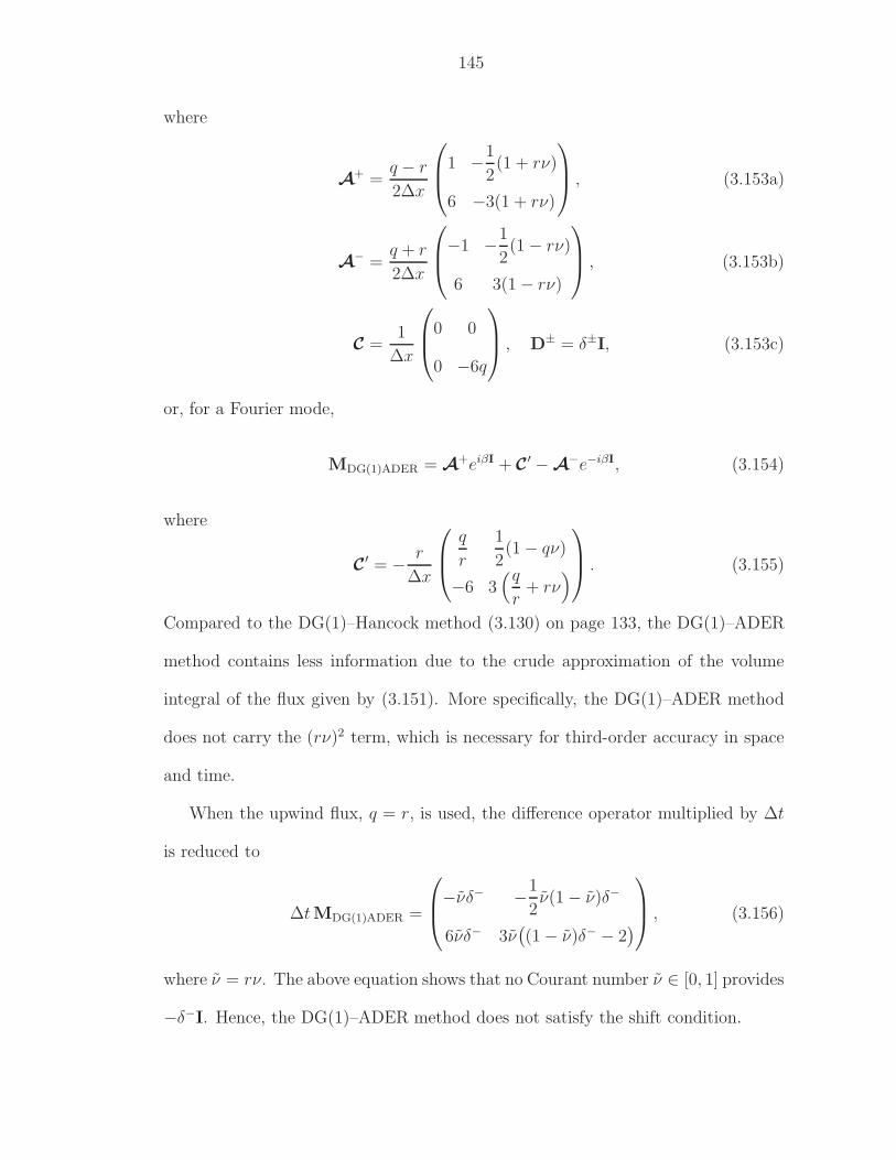
145
where
A+ =
q − r
2∆x
1 −1
2(1 + rν)
6 −3(1 + rν)
, (3.153a)
A− =
q + r
2∆x
−1 −1
2(1 − rν)
6 3(1 − rν)
, (3.153b)
C =1
∆x
0 0
0 −6q
, D± = δ±I, (3.153c)
or, for a Fourier mode,
MDG(1)ADER = A+eiβI + C
′ − A−e−iβI, (3.154)
where
C′ = − r
∆x
q
r
1
2(1 − qν)
−6 3(q
r+ rν
)
. (3.155)
Compared to the DG(1)–Hancock method (3.130) on page 133, the DG(1)–ADER
method contains less information due to the crude approximation of the volume
integral of the flux given by (3.151). More specifically, the DG(1)–ADER method
does not carry the (rν)2 term, which is necessary for third-order accuracy in space
and time.
When the upwind flux, q = r, is used, the difference operator multiplied by ∆t
is reduced to
∆tMDG(1)ADER =
−νδ− −1
2ν(1 − ν)δ−
6νδ− 3ν((1 − ν)δ− − 2
)
, (3.156)
where ν = rν. The above equation shows that no Courant number ν ∈ [0, 1] provides
−δ−I. Hence, the DG(1)–ADER method does not satisfy the shift condition.
146
To obtained the local truncation error, the forward Euler method is adopted for
the time integration:
GDG(1)ADER = I + ∆tMDG(1)ADER. (3.157)
Accuracy Following the same procedure, the local truncation error of the
method becomes
LTE(1)DG(1)ADER = λ
(1)DG(1)ADER − λexact
= − ir
12rν
(r
q− rν
)∆x2 k3
− r
72
r
q
[1 − 4
r
q(rν) + 3(rν)2
]∆x3k4 + O
(k5).
(3.158a)
Thus, the DG(1)–ADER method is second-order accurate in space and time.
Stability The modulus of the amplification factor, |gDG(1)ADER(ν, β)|, computed
with the upwind flux, is shown in Figure 3.13. In contrast to the SV2–RK2 method,
the dissipation property of the DG(1)–ADER method is qualitatively similar to
that of DG(1)–Hancock method shown in Figure 3.10 on page 137. However, the
DG(1)–ADER method is second-order accurate and the stability domain is more
restrictive, ν ≤ 1
3, whereas the DG(1)–Hancock method is third-order accurate
while stable for ν ≤ 1.
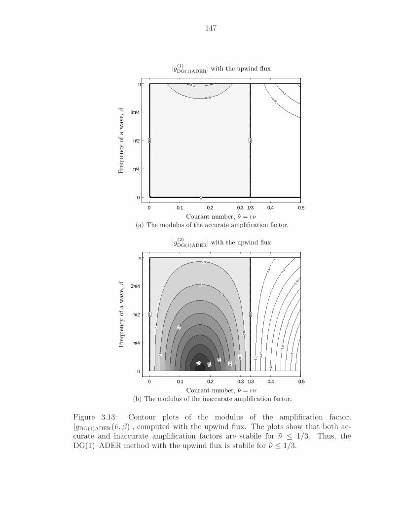
147
0 0.1 0.2 0.3 1/3 0.4 0.5
0
π/4
π/2
3π/4
π 0.92
0.95 1.05
1.1
1
1
1
Courant number, ν = rν
Fre
quen
cyofa
wav
e,β
|g(1)DG(1)ADER| with the upwind flux
(a) The modulus of the accurate amplification factor.
0 0.1 0.2 0.3 1/3 0.4 0.5
0
π/4
π/2
3π/4
π
0.1 0.2
0.4 0.6
0.6
0.8
0.8
0.8
0.9
0.9
0.9
1.1
1.1
1.2
1.2
1.4
1.4
1.6
1.8
11
Courant number, ν = rν
Fre
quen
cyofa
wav
e,β
|g(2)DG(1)ADER| with the upwind flux
(b) The modulus of the inaccurate amplification factor.
Figure 3.13: Contour plots of the modulus of the amplification factor,|gDG(1)ADER(ν, β)|, computed with the upwind flux. The plots show that both ac-curate and inaccurate amplification factors are stabile for ν ≤ 1/3. Thus, theDG(1)–ADER method with the upwind flux is stabile for ν ≤ 1/3.
148
3.3.6 Dominant Dispersion/Dissipation Error and Stability in 1-D
The results of a Fourier analysis for each method are listed below for compar-
ison. The details of the HR3–RK3, DG(2)–RK3, and DG(2)–ADER methods are
presented in Appendix B on page 349. The local truncation errors show the domi-
nant dispersion error, O(k3)-term, and the dissipation error, O(k4)-term. Moreover,
owing to the equivalence of the Fourier analysis and the modified-equation analysis,
the leading error term indicates the order of accuracy. Note that c3 ∝ ∆x2 and
c4 ∝ ∆x3.
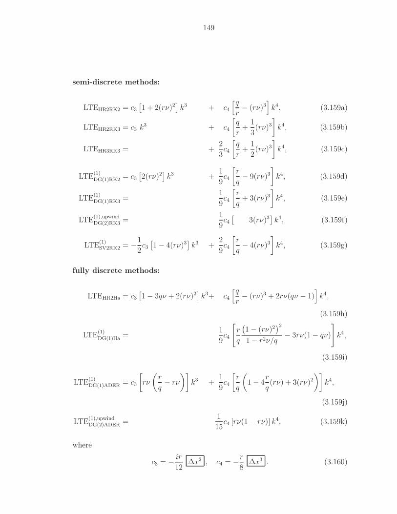
149
semi-discrete methods:
LTEHR2RK2 = c3
[1 + 2(rν)2
]k3 + c4
[qr− (rν)3
]k4, (3.159a)
LTEHR2RK3 = c3 k3 + c4
[q
r+
1
3(rν)3
]k4, (3.159b)
LTEHR3RK3 = +2
3c4
[q
r+
1
2(rν)3
]k4, (3.159c)
LTE(1)DG(1)RK2 = c3
[2(rν)2
]k3 +
1
9c4
[r
q− 9(rν)3
]k4, (3.159d)
LTE(1)DG(1)RK3 =
1
9c4
[r
q+ 3(rν)3
]k4, (3.159e)
LTE(1),upwindDG(2)RK3 =
1
9c4
[3(rν)3
]k4, (3.159f)
LTE(1)SV2RK2 = −1
2c3
[1 − 4(rν)3
]k3 +
2
9c4
[r
q− 4(rν)3
]k4, (3.159g)
fully discrete methods:
LTEHR2Ha = c3
[1 − 3qν + 2(rν)2
]k3+ c4
[qr− (rν)3 + 2rν(qν − 1)
]k4,
(3.159h)
LTE(1)DG(1)Ha =
1
9c4
[r
q
(1 − (rν)2
)2
1 − r2ν/q− 3rν(1 − qν)
]k4,
(3.159i)
LTE(1)DG(1)ADER = c3
[rν
(r
q− rν
)]k3 +
1
9c4
[r
q
(1 − 4
r
q(rν) + 3(rν)2
)]k4,
(3.159j)
LTE(1),upwindDG(2)ADER =
1
15c4 [rν(1 − rν)] k4, (3.159k)
where
c3 = − ir
12∆x2 , c4 = −r
8∆x3 . (3.160)
150
The above equations show that the leading errors of the HR3–RK3, DG(1)–RK3,
DG(2)–RK3, DG(1)–Hancock, and DG(2)–ADER methods are O(∆x3), whereas in
the rest of methods they are O(∆x2). Interestingly, the DG(1) spatial discretization
can yield a third-order method, at least for a linear equation discretized on a uni-
form grid, if a proper time integration method is adopted. The Hancock and RK3
method lead to a third-order method; note that, DG(1)–RK3 requires three flux
calculations at each cell-interface whereas DG(1)–Hancock requires two to achieve
the same order. The DG(2) spatial discretization together with the same (third)
order of temporal discretization provides a third-order method: DG(2)–RK3 and
DG(2)–ADER. In these methods, the leading error can be attributed to the tempo-
ral discretization, as can be seen by letting ν = rν → 0 : the O(k4)-term disappears.
The analysis also shows the lower dissipation of DG discretizations: the leading-
error coefficient of a DG(1) method is1
9of the value for HR2,
1
6of the value for
HR3, and1
2of the value for SV2.
The stability limits of the methods when combined with the upwind and Lax–
Friedrichs fluxes are shown in Table 3.3. In an HR (finite-volume) method, the
linear stability limit increases as the order of method increases due to the inclusion
of wider stencils. Conversely, DG and SV methods reduce their stability domain
while increasing the order of accuracy, because increasing the number of unknowns
per cell is equivalent to a grid refinement. This suggests that the inaccurate (second)
amplification factor indeed contributes to the accuracy, but on the subgrid scale.
In order to understand the grid-refinement phenomena of the DG and SV methods,
previously presented stability domains are reproduced over the domain β ∈ [0, 2π],
and shown in Figure 3.14. For each method, the accurate amplification factor is
plotted over β ∈ [0, π], while the inaccurate one is plotted for β ∈ [π, 2π]. A smooth
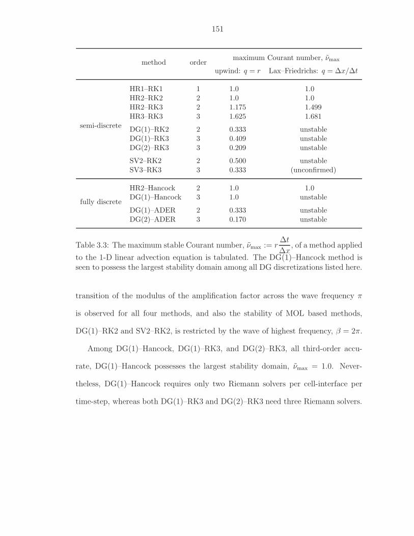
151
method ordermaximum Courant number, νmax
upwind: q = r Lax–Friedrichs: q = ∆x/∆t
semi-discrete
HR1–RK1 1 1.0 1.0HR2–RK2 2 1.0 1.0HR2–RK3 2 1.175 1.499HR3–RK3 3 1.625 1.681
DG(1)–RK2 2 0.333 unstableDG(1)–RK3 3 0.409 unstableDG(2)–RK3 3 0.209 unstable
SV2–RK2 2 0.500 unstableSV3–RK3 3 0.333 (unconfirmed)
fully discrete
HR2–Hancock 2 1.0 1.0DG(1)–Hancock 3 1.0 unstable
DG(1)–ADER 2 0.333 unstableDG(2)–ADER 3 0.170 unstable
Table 3.3: The maximum stable Courant number, νmax := r∆t
∆x, of a method applied
to the 1-D linear advection equation is tabulated. The DG(1)–Hancock method isseen to possess the largest stability domain among all DG discretizations listed here.
transition of the modulus of the amplification factor across the wave frequency π
is observed for all four methods, and also the stability of MOL based methods,
DG(1)–RK2 and SV2–RK2, is restricted by the wave of highest frequency, β = 2π.
Among DG(1)–Hancock, DG(1)–RK3, and DG(2)–RK3, all third-order accu-
rate, DG(1)–Hancock possesses the largest stability domain, νmax = 1.0. Never-
theless, DG(1)–Hancock requires only two Riemann solvers per cell-interface per
time-step, whereas both DG(1)–RK3 and DG(2)–RK3 need three Riemann solvers.
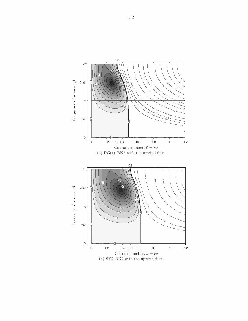
152
0 0.2 1/3 0.4 0.6 0.8 1 1.20
π/2
π
3π/2
2π
0.8
0.9
0.95
1.2
1.2
1.41.6
2
3
45
6
1
1
1
0.6
0.6
0.8 1.21.4 2
4
6
8
100.8
1
1
1/3
Courant number, ν = rν
Fre
quen
cyofa
wav
e,β
(a) DG(1)–RK2 with the upwind flux
0 0.2 0.4 0.5 0.6 0.8 1 1.20
π/2
π
3π/2
2π
0.7
0.8
0.9
0.95
1.21
1
1
0.6
0.8
0.91.21.4
2 3 4
0.4
0.8
6
0.9
0.2 11
0.5
Courant number, ν = rν
Fre
quen
cyofa
wav
e,β
(b) SV2–RK2 with the upwind flux
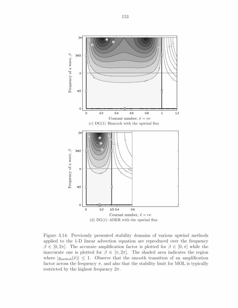
153
0 0.2 0.4 0.6 0.8 1 1.20
π/2
π
3π/2
2π
0.90.95
0.95
1.11.2
1
1
1
0.2
0.4
0.6
0.8
0.8
0.9
0.95 1.2
1.4
1.6
0.9
1.82
0.95
11
Courant number, ν = rν
Fre
quen
cyofa
wav
e,β
(c) DG(1)–Hancock with the upwind flux
0 0.2 1/3 0.4 0.60
π/2
π
3π/2
2π
0.951.1
1.21.3
1
1
1
0.2
0.4
0.6
0.80.8
0.9
0.9
1.11.2 1.4
2
11
Courant number, ν = rν
Fre
quen
cyofa
wav
e,β
(d) DG(1)–ADER with the upwind flux
Figure 3.14: Previously presented stability domains of various upwind methodsapplied to the 1-D linear advection equation are reproduced over the frequencyβ ∈ [0, 2π]. The accurate amplification factor is plotted for β ∈ [0, π] while theinaccurate one is plotted for β ∈ [π, 2π]. The shaded area indicates the regionwhere |gmethod(ν)| ≤ 1. Observe that the smooth transition of an amplificationfactor across the frequency π, and also that the stability limit for MOL is typicallyrestricted by the highest frequency 2π.
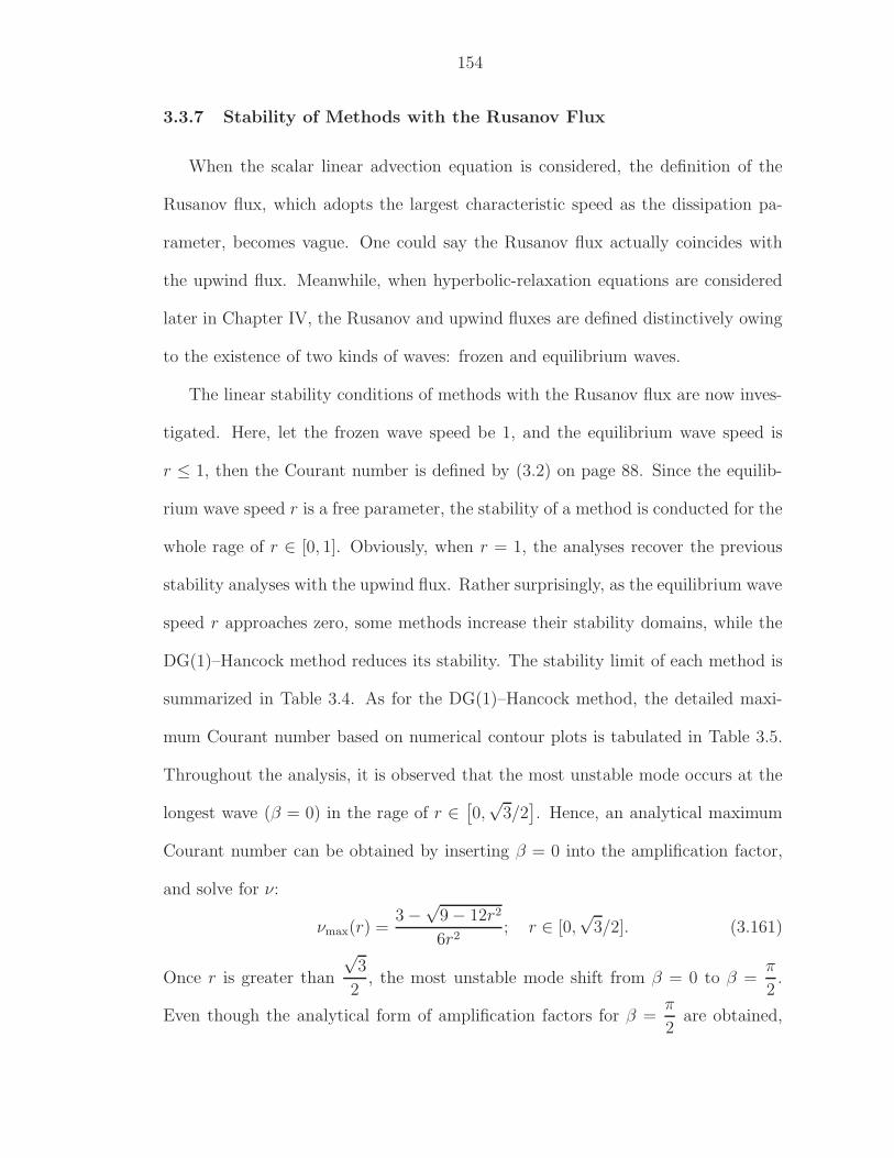
154
3.3.7 Stability of Methods with the Rusanov Flux
When the scalar linear advection equation is considered, the definition of the
Rusanov flux, which adopts the largest characteristic speed as the dissipation pa-
rameter, becomes vague. One could say the Rusanov flux actually coincides with
the upwind flux. Meanwhile, when hyperbolic-relaxation equations are considered
later in Chapter IV, the Rusanov and upwind fluxes are defined distinctively owing
to the existence of two kinds of waves: frozen and equilibrium waves.
The linear stability conditions of methods with the Rusanov flux are now inves-
tigated. Here, let the frozen wave speed be 1, and the equilibrium wave speed is
r ≤ 1, then the Courant number is defined by (3.2) on page 88. Since the equilib-
rium wave speed r is a free parameter, the stability of a method is conducted for the
whole rage of r ∈ [0, 1]. Obviously, when r = 1, the analyses recover the previous
stability analyses with the upwind flux. Rather surprisingly, as the equilibrium wave
speed r approaches zero, some methods increase their stability domains, while the
DG(1)–Hancock method reduces its stability. The stability limit of each method is
summarized in Table 3.4. As for the DG(1)–Hancock method, the detailed maxi-
mum Courant number based on numerical contour plots is tabulated in Table 3.5.
Throughout the analysis, it is observed that the most unstable mode occurs at the
longest wave (β = 0) in the rage of r ∈[0,√
3/2]. Hence, an analytical maximum
Courant number can be obtained by inserting β = 0 into the amplification factor,
and solve for ν:
νmax(r) =3 −
√9 − 12r2
6r2; r ∈ [0,
√3/2]. (3.161)
Once r is greater than
√3
2, the most unstable mode shift from β = 0 to β =
π
2.
Even though the analytical form of amplification factors for β =π
2are obtained,
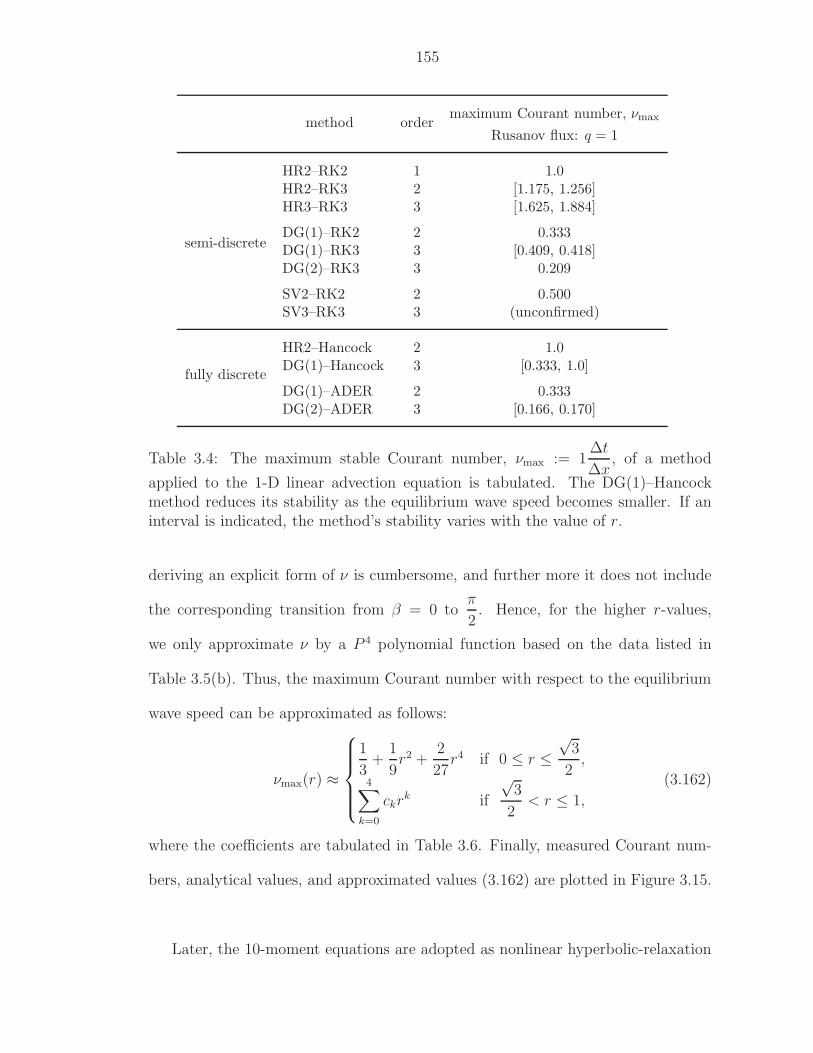
155
method ordermaximum Courant number, νmax
Rusanov flux: q = 1
semi-discrete
HR2–RK2 1 1.0HR2–RK3 2 [1.175, 1.256]HR3–RK3 3 [1.625, 1.884]
DG(1)–RK2 2 0.333DG(1)–RK3 3 [0.409, 0.418]DG(2)–RK3 3 0.209
SV2–RK2 2 0.500SV3–RK3 3 (unconfirmed)
fully discrete
HR2–Hancock 2 1.0DG(1)–Hancock 3 [0.333, 1.0]
DG(1)–ADER 2 0.333DG(2)–ADER 3 [0.166, 0.170]
Table 3.4: The maximum stable Courant number, νmax := 1∆t
∆x, of a method
applied to the 1-D linear advection equation is tabulated. The DG(1)–Hancockmethod reduces its stability as the equilibrium wave speed becomes smaller. If aninterval is indicated, the method’s stability varies with the value of r.
deriving an explicit form of ν is cumbersome, and further more it does not include
the corresponding transition from β = 0 toπ
2. Hence, for the higher r-values,
we only approximate ν by a P 4 polynomial function based on the data listed in
Table 3.5(b). Thus, the maximum Courant number with respect to the equilibrium
wave speed can be approximated as follows:
νmax(r) ≈
1
3+
1
9r2 +
2
27r4 if 0 ≤ r ≤
√3
2,
4∑
k=0
ckrk if
√3
2< r ≤ 1,
(3.162)
where the coefficients are tabulated in Table 3.6. Finally, measured Courant num-
bers, analytical values, and approximated values (3.162) are plotted in Figure 3.15.
Later, the 10-moment equations are adopted as nonlinear hyperbolic-relaxation
156
(a) r ∈[0,√
3/2]
r νmax(r)
0.0 1/30.1 0.3350.2 0.3380.3 0.3440.4 0.3530.5 0.3670.6 0.3870.7 0.4200.8 0.4820.82 0.5040.84 0.5360.85 0.5600.86 0.5960.865 0.636√
3/2 ∼ 0.866 2/3 ∼ 0.667
(b) r ∈[√
3/2, 1]
r νmax(r)
0.866 0.7580.87 0.7870.88 0.8280.90 0.8770.92 0.9120.94 0.9390.96 0.9620.98 0.9821.0 1.0
Table 3.5: The allowable maximum Courant number with respect to the equilibriumwave speed r ∈ [0, 1] for the DG(1)–Hancock method with the Rusanov flux istabulated. These values are measured based on contour plots of the modulus ofamplification factors. When r = 1, the result recovers the stability with the upwindflux, while the stability domain is reduced towards 1/3 as the equilibrium wave getssmaller.
equations. This system has a dimensionless wave speed defined by
r(M) :=u + a
u +√
3a=
M + 1
M +√
3, (3.163)
hence, as the Mach number increases, the maximum stable Courant number also
relaxes towards unity. The transition of the Courant number with respect to r is
shown in Figure 3.16.
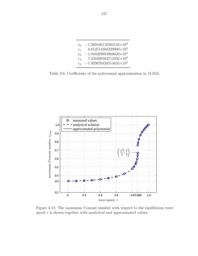
157
c0 −1.569446110504144×10³
c1 6.612514388329900×10³
c2 −1.044389804968620×10⁴
c3 7.331699503711032×10³
c4 −1.929870438514635×10³
Table 3.6: Coefficients of the polynomial approximation in (3.162).
0 0.2 0.4 0.6 0.8 0.866 1.0 0.2
1/3
0.4
0.5
0.6
0.7
0.8
0.9
1.0
(√3
2,2
3
)−→
measured valuesanalytical solutionapproximated polynomial
wave speed, r
maxum
um
Coura
nt
num
ber
,ν m
ax
Figure 3.15: The maximum Courant number with respect to the equilibrium wavespeed r is shown together with analytical and approximated values.
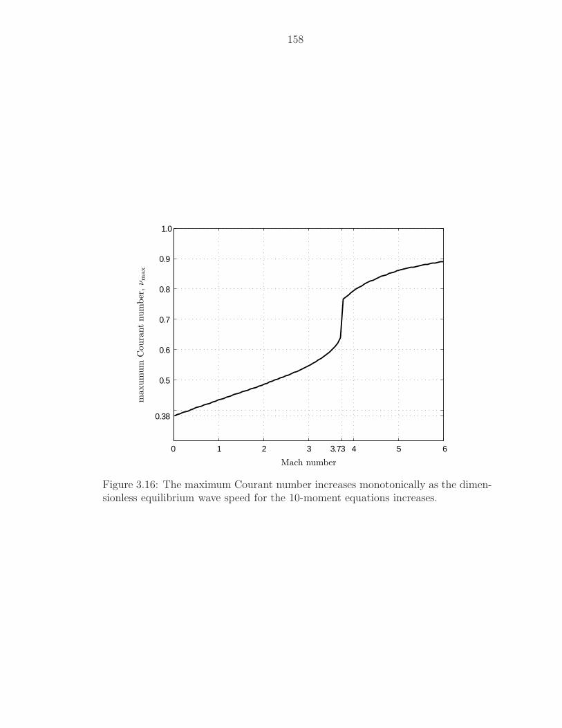
158
0 1 2 3 3.73 4 5 6
0.38
0.5
0.6
0.7
0.8
0.9
1.0
Mach number
maxum
um
Coura
nt
num
ber
,ν m
ax
Figure 3.16: The maximum Courant number increases monotonically as the dimen-sionless equilibrium wave speed for the 10-moment equations increases.
159
3.4 Difference Operators and Their Properties in 2-D
In this section, several discretization methods are applied to the two-dimensional
linear advection equation (3.1b), and a Fourier analysis is employed to uncover their
dominant dissipation and dispersion errors, order of accuracy, and domain of linear
stability. Four methods, HR2–RK2, HR2–Hancock, DG(1)–RK2, and DG(1)–RK3,
are compared to the DG(1)–Hancock method. To simplify the analysis, we only
consider rectangular grids here; the extension of a Fourier analysis on quadrilateral
and triangular grids is shown by Huynh [Huy03] for the upwind (Hancock) and some
centered staggered methods.
To write a method in compact form, the difference operators in the x-,y-directions
are defined as follows:
δ+x ui,j = ui+1,j − ui,j, δ−x ui,j = ui,j − ui−1,j , (3.164a)
δ+y ui,j = ui,j+1 − ui,j, δ−y ui,j = ui,j − ui,j−1. (3.164b)
Even though the multi-dimensional problem is considered, Godunov-type and DG
methods utilize a one-dimensional Riemann solver. Let uE and uW be the point
values on either side of a cell face normal to the x-direction, and uN and uS at the
cell faces normal to the y-direction. Then, the interface fluxes in the x-,y-directions
are given by
f qi+1/2,j(uW , uE) =
r
2(uE + uW ) − qx
2(uE − uW ), (3.165a)
gqi,j+1/2(uS, uN) =
s
2(uN + uS) − qy
2(uN − uS), (3.165b)
160
where
upwind : (qx, qy) = (|r|, |s|), (3.166a)
Rusanov: (qx, qy) = (1, 1), (3.166b)
Lax–Friedrichs : (qx, qy) =
(∆x
∆t,∆y
∆t
). (3.166c)
Note that the 1-D Lax–Friedrichs flux does not produce the original 2-D Lax–Friedrichs
scheme formulated for a staggered grid. In fact, the Lax–Friedrichs flux contains
too much dissipation for a 2-D calculation and causes a high-frequency instability,
even in a first-order method. We will therefore not apply the Lax–Friedrichs flux
beyond one dimension.
The exact solution of (3.1b) for a harmonic mode is
u(x, y, t) = u0eikx(x−rt)eiky(y−st), (3.167)
where (kx, ky) are the wave numbers in (x, y). The exact amplification factor is
obtained by inserting the time increment, t + ∆t, into the above equation, then
insert u(x, t):
u(x, t + ∆t) = e−i(rkx+sky)∆t u(x, t). (3.168)
Hence, the exact amplification factor and exact eigenvalue of the spatial differenti-
ation in the time step, ∆t, are given by
gexact = e−i(rkx+sky)∆t, (3.169a)
λexact = −i(rkx + sky). (3.169b)
Since the wave numbers (kx, ky) are related to the spatial frequencies of a wave in
the x-, and y-directions, (α, β), such that
(kx, ky) =
(α
∆x,
β
∆y
), (3.170)
161
the exact amplification factor and exact eigenvalue of 2-D spatial differentiation can
be expressed as
gexact(νx, νy, α, β) = e−i(rνxα+sνyβ) = e−i(νxα+νyβ), (3.171a)
λexact = −i
(r
∆xα +
s
∆yβ
). (3.171b)
The exact amplification factor in the low-frequency limit is given by expanding in
the frequencies of a wave, (α, β), at fixed Courant numbers, (rνx, sνy), thus
gexact(rνx, sνy, α, β) =
[1 + (−irνx)α +
1
2(−irνx)
2α2 + O(α3)]
×[1 + (−isνy)β +
1
2(−isνy)
2β2 + O(β3)]
. (3.172)
The asymptotic expansion is further simplified when the wave speeds in the x-,y-
directions are the same, s = r, and we also set νx = νy = ν; then
gexact(rν, β) = 1 + 2(−irν)β + 2(−irν)2β2 +4
3(−irν)3β3 +
2
3(−irν)4β4 + O
(β5).
(3.173)
Accuracy
The local truncation error of a multi-dimensional method is obtained by straight-
forward extension of the one-dimensional analysis [CdLBL97, Ram94], described in
the previous section. A Taylor series expansion of a space-time eigenvalue, λmethod,
around kx = ky = 0 leads to a local truncation error:
LTEmethod = λmethod − λexact
=1
∆tln g(rνx, sνy, kx, ky) − λexact
=∞∑
m,n=2
cm,nkmx kn
y , (3.174)
162
where the coefficient of the modified equation, cm,n is given by
cm,n =1
m! n!
∂m+nλ
∂kmx ∂kn
y
∣∣∣∣kx,ky=0
=1
m! n!∆tg(kx, ky = 0)
∂m+ng(kx, ky)
∂kmx ∂kn
y
∣∣∣∣kx,ky=0
. (3.175)
In the one-dimensional analysis, the polar form of an amplification factor is obtained
first, then a local truncation error is derived. However, in the two-dimensional
case, a local truncation error is directly obtained by the above equation due to the
complexity of deriving the polar form of the amplification factor.
Stability
A single Courant number for a two-dimensional problem on rectangular grids
can not be uniquely defined; most often used in practice is the definition
ν2D := νx + νy
= r∆t
∆x+ s
∆t
∆y. (3.176)
This choice is explained in some detail in Chapter V, as it derives from the more
general form (5.13). Following a procedure similar to the one-dimensional analysis,
the linear stability conditions of various methods with the upwind flux is obtained
numerically.
As a preliminary analysis, the stability domains of the first-order method with
the upwind flux is considered. The maximum modulus of the amplification factor
|g1st-order|max over β ∈ [0, π] at the Courant numbers νx, νy ∈ [0, 1] is shown in
Figure 3.17. The shaded area represents the stable region: |g1st-order| ≤ 1 for any
β ∈ [0, π]. Based on the numerical results, the stability domain for the upwind flux
is given by
νupwind2D, 1st-order = νx + νy ≤ 1.0. (3.177)
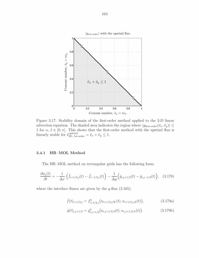
163
0 0.2 0.4 0.6 0.8 10
0.2
0.4
0.6
0.8
1
1
1
1
νx + νy ≤ 1
Courant number, νx = rνx
Coura
nt
num
ber
,ν y
=sν
y
|g1st-order| with the upwind flux
Figure 3.17: Stability domain of the first-order method applied to the 2-D linearadvection equation. The shaded area indicates the region where |gfirst-order(νx, νy)| ≤1 for α, β ∈ [0, π]. This shows that the first-order method with the upwind flux islinearly stable for νupwind
2D, 1st-order = νx + νy ≤ 1.
3.4.1 HR–MOL Method
The HR–MOL method on rectangular grids has the following form:
∂uj(t)
∂t= − 1
∆x
(fi+1/2,j(t) − fi−1/2,j(t)
)− 1
∆y
(gi,j+1/2(t) − gi,j−1/2(t)
), (3.178)
where the interface fluxes are given by the q-flux (3.165):
f(t)i+1/2,j = f qi+1/2,j
(ui+1/2,j,W (t), ui+1/2,j,E(t)
), (3.179a)
g(t)i,j+1/2 = gqi,j+1/2
(ui,j+1/2,S(t), ui,j+1/2,N(t)
). (3.179b)
164
The input values for the q-flux are obtained by
ui+1/2,j,W = ui,j +1
2∆xui,j, ui+1/2,j,E = ui+1,j −
1
2∆xui+1,j, (3.180a)
ui+1/2,j,S = ui,j +1
2∆yui,j, ui+1/2,j,N = ui,j+1 −
1
2∆yui,j+1, (3.180b)
where, just as the 1-D analysis, the slopes are obtained by the difference over the
domain (i + 1, i, i − 1) in the x-direction, and (j + 1, j, j − 1) in the y-direction
respectively:
∆xui,j =1
2(ui+1,j − ui−1,j), (3.181a)
∆yui,j =1
2(ui,j+1 − ui,j−1). (3.181b)
After inserting these difference formulas into the semi-discrete method (3.178), and
some algebra, the spatial difference operator of the HR2–MOL becomes
∂uj(t)
∂t= NHR2uj(t), (3.182)
where
NHR2 =
2∑
m=1
[a1m(δ+
x )m + a2m(δ−x )m + b1m(δ+y )m + b2m(δ−y )m
]. (3.183)
Here, the coefficients of the difference operator NHR2 are given by
a11 a12
a21 a22
= − 1
8∆x
2(2r − qx) qx − r
2(2r + qx) qx + r
, (3.184a)
b11 b12
b21 b22
= − 1
8∆y
2(2s − qy) qy − s
2(2s + qy) qy + s
. (3.184b)
Accuracy Taking the low-frequency limit of the difference spatial operator NHR2
leads to the asymptotic eigenvalue:
λHR2 = −i
(r
∆xα +
s
∆yβ
)− i
12
(r
∆xα3 +
s
∆yβ3
)−1
8
(qx
∆xα4 +
qy
∆yβ4
)+O(α5, β5
).
(3.185)
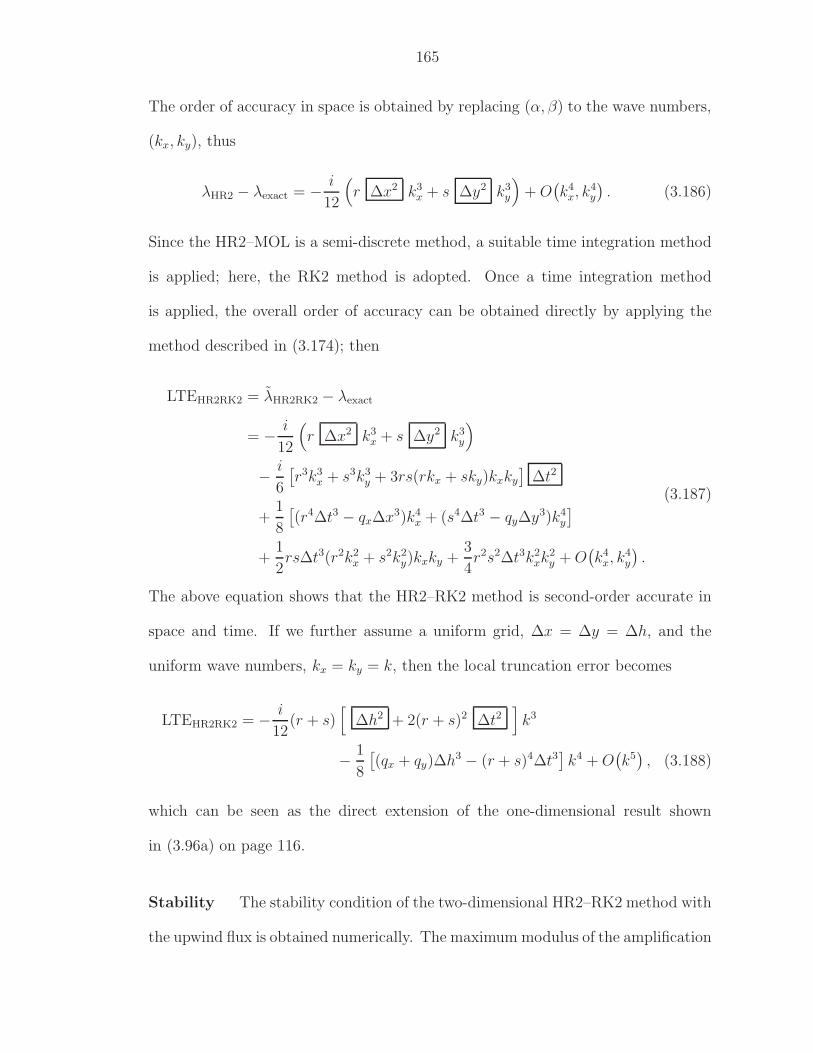
165
The order of accuracy in space is obtained by replacing (α, β) to the wave numbers,
(kx, ky), thus
λHR2 − λexact = − i
12
(r ∆x2 k3
x + s ∆y2 k3y
)+ O
(k4
x, k4y
). (3.186)
Since the HR2–MOL is a semi-discrete method, a suitable time integration method
is applied; here, the RK2 method is adopted. Once a time integration method
is applied, the overall order of accuracy can be obtained directly by applying the
method described in (3.174); then
LTEHR2RK2 = λHR2RK2 − λexact
= − i
12
(r ∆x2 k3
x + s ∆y2 k3y
)
− i
6
[r3k3
x + s3k3y + 3rs(rkx + sky)kxky
]∆t2
+1
8
[(r4∆t3 − qx∆x3)k4
x + (s4∆t3 − qy∆y3)k4y
]
+1
2rs∆t3(r2k2
x + s2k2y)kxky +
3
4r2s2∆t3k2
xk2y + O
(k4
x, k4y
).
(3.187)
The above equation shows that the HR2–RK2 method is second-order accurate in
space and time. If we further assume a uniform grid, ∆x = ∆y = ∆h, and the
uniform wave numbers, kx = ky = k, then the local truncation error becomes
LTEHR2RK2 = − i
12(r + s)
[∆h2 + 2(r + s)2 ∆t2
]k3
− 1
8
[(qx + qy)∆h3 − (r + s)4∆t3
]k4 + O
(k5), (3.188)
which can be seen as the direct extension of the one-dimensional result shown
in (3.96a) on page 116.
Stability The stability condition of the two-dimensional HR2–RK2 method with
the upwind flux is obtained numerically. The maximum modulus of the amplification
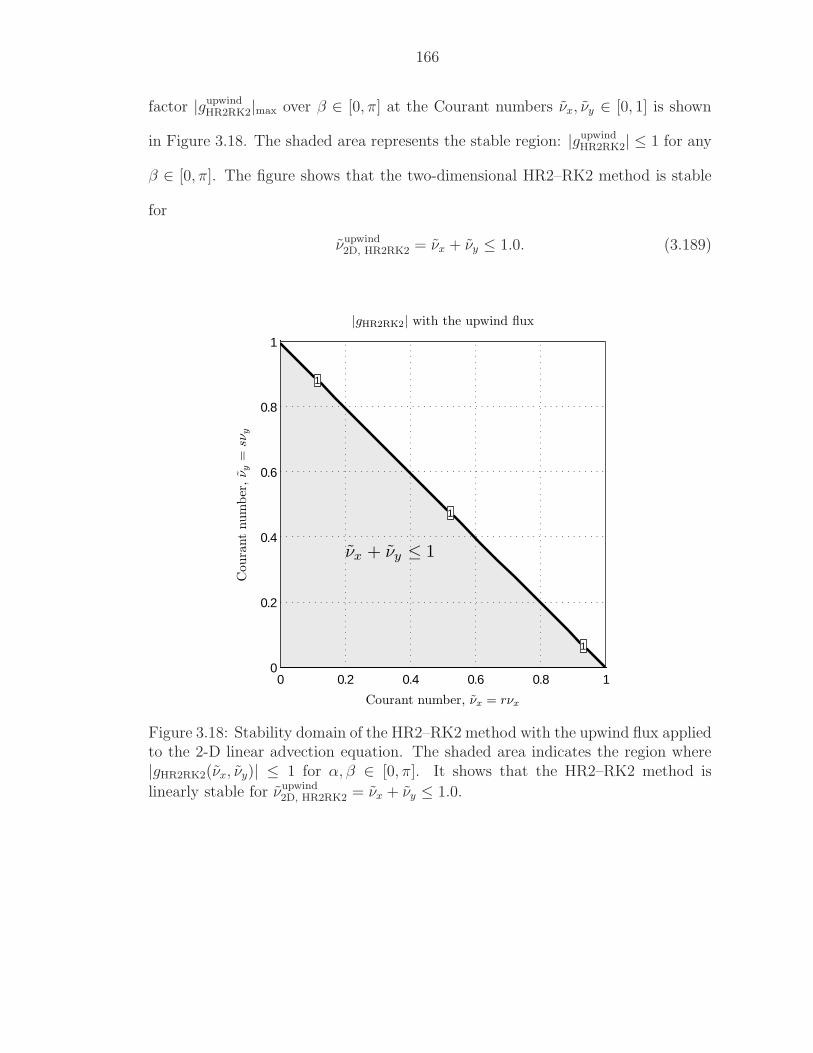
166
factor |gupwindHR2RK2|max over β ∈ [0, π] at the Courant numbers νx, νy ∈ [0, 1] is shown
in Figure 3.18. The shaded area represents the stable region: |gupwindHR2RK2| ≤ 1 for any
β ∈ [0, π]. The figure shows that the two-dimensional HR2–RK2 method is stable
for
νupwind2D, HR2RK2 = νx + νy ≤ 1.0. (3.189)
0 0.2 0.4 0.6 0.8 10
0.2
0.4
0.6
0.8
1
1
1
1
νx + νy ≤ 1
Courant number, νx = rνx
Coura
nt
num
ber
,ν y
=sν
y
|gHR2RK2| with the upwind flux
Figure 3.18: Stability domain of the HR2–RK2 method with the upwind flux appliedto the 2-D linear advection equation. The shaded area indicates the region where|gHR2RK2(νx, νy)| ≤ 1 for α, β ∈ [0, π]. It shows that the HR2–RK2 method is
linearly stable for νupwind2D, HR2RK2 = νx + νy ≤ 1.0.
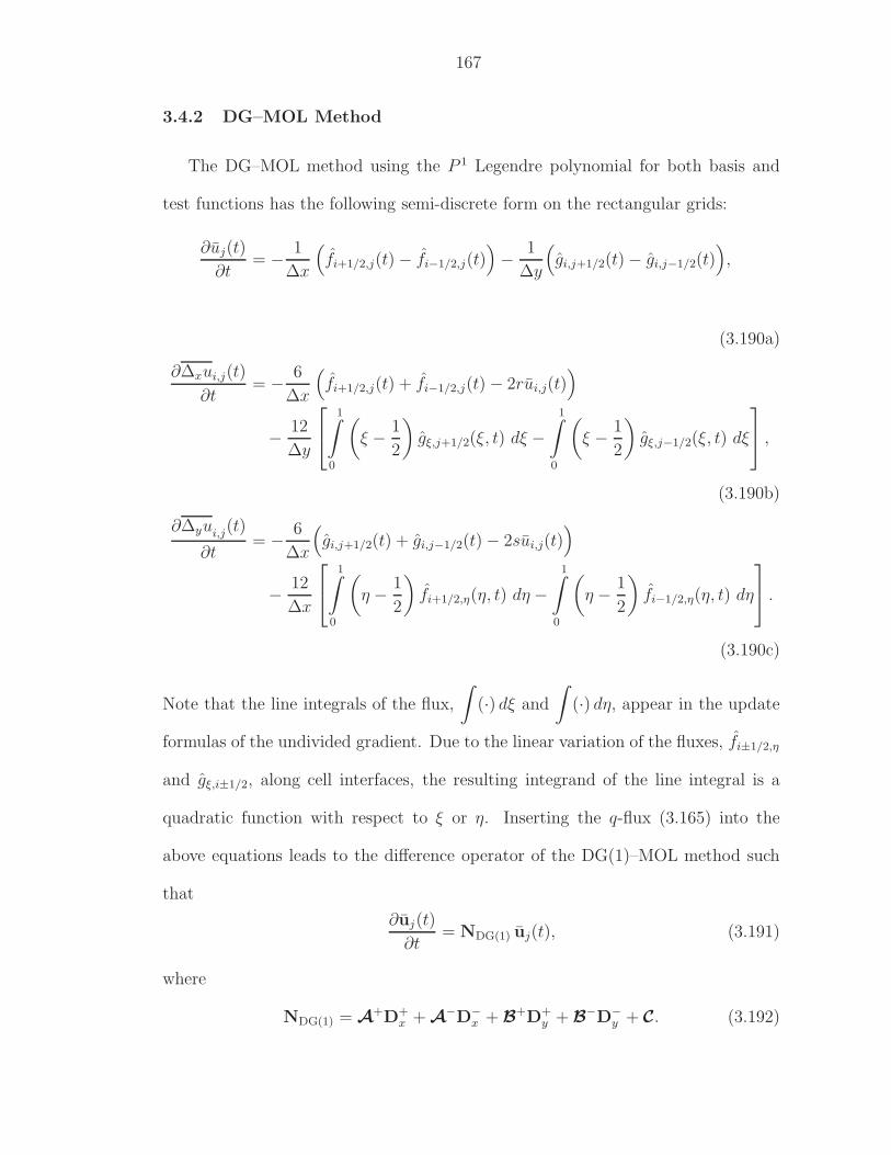
167
3.4.2 DG–MOL Method
The DG–MOL method using the P 1 Legendre polynomial for both basis and
test functions has the following semi-discrete form on the rectangular grids:
∂uj(t)
∂t= − 1
∆x
(fi+1/2,j(t) − fi−1/2,j(t)
)− 1
∆y
(gi,j+1/2(t) − gi,j−1/2(t)
),
(3.190a)
∂∆xui,j(t)
∂t= − 6
∆x
(fi+1/2,j(t) + fi−1/2,j(t) − 2rui,j(t)
)
− 12
∆y
1∫
0
(ξ − 1
2
)gξ,j+1/2(ξ, t) dξ −
1∫
0
(ξ − 1
2
)gξ,j−1/2(ξ, t) dξ
,
(3.190b)
∂∆yui,j(t)
∂t= − 6
∆x
(gi,j+1/2(t) + gi,j−1/2(t) − 2sui,j(t)
)
− 12
∆x
1∫
0
(η − 1
2
)fi+1/2,η(η, t) dη −
1∫
0
(η − 1
2
)fi−1/2,η(η, t) dη
.
(3.190c)
Note that the line integrals of the flux,
∫(·) dξ and
∫(·) dη, appear in the update
formulas of the undivided gradient. Due to the linear variation of the fluxes, fi±1/2,η
and gξ,i±1/2, along cell interfaces, the resulting integrand of the line integral is a
quadratic function with respect to ξ or η. Inserting the q-flux (3.165) into the
above equations leads to the difference operator of the DG(1)–MOL method such
that
∂uj(t)
∂t= NDG(1) uj(t), (3.191)
where
NDG(1) = A+D+
x + A−D−
x + B+D+
y + B−D−
y + C. (3.192)
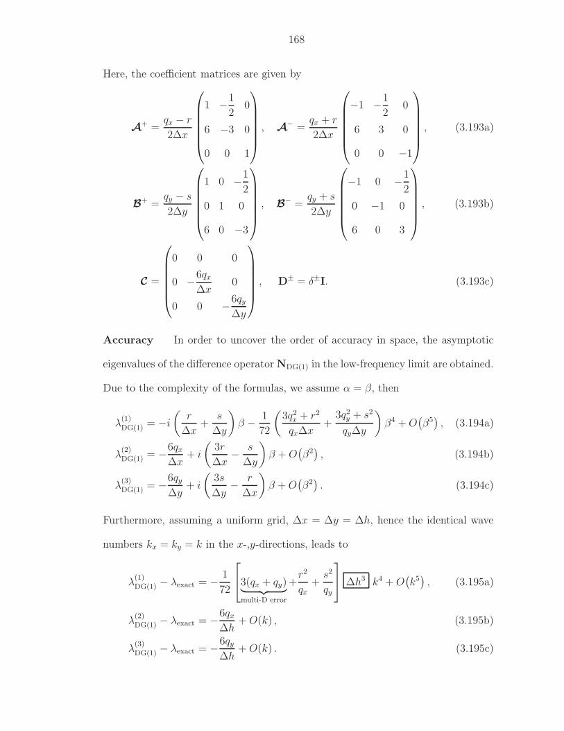
168
Here, the coefficient matrices are given by
A+ =
qx − r
2∆x
1 −1
20
6 −3 0
0 0 1
, A− =
qx + r
2∆x
−1 −1
20
6 3 0
0 0 −1
, (3.193a)
B+ =
qy − s
2∆y
1 0 −1
2
0 1 0
6 0 −3
, B− =
qy + s
2∆y
−1 0 −1
2
0 −1 0
6 0 3
, (3.193b)
C =
0 0 0
0 −6qx
∆x0
0 0 −6qy
∆y
, D± = δ±I. (3.193c)
Accuracy In order to uncover the order of accuracy in space, the asymptotic
eigenvalues of the difference operator NDG(1) in the low-frequency limit are obtained.
Due to the complexity of the formulas, we assume α = β, then
λ(1)DG(1) = −i
(r
∆x+
s
∆y
)β − 1
72
(3q2
x + r2
qx∆x+
3q2y + s2
qy∆y
)β4 + O
(β5), (3.194a)
λ(2)DG(1) = −6qx
∆x+ i
(3r
∆x− s
∆y
)β + O
(β2), (3.194b)
λ(3)DG(1) = −6qy
∆y+ i
(3s
∆y− r
∆x
)β + O
(β2). (3.194c)
Furthermore, assuming a uniform grid, ∆x = ∆y = ∆h, hence the identical wave
numbers kx = ky = k in the x-,y-directions, leads to
λ(1)DG(1) − λexact = − 1
72
3(qx + qy)︸ ︷︷ ︸
multi-D error
+r2
qx+
s2
qy
∆h3 k4 + O
(k5), (3.195a)
λ(2)DG(1) − λexact = −6qx
∆h+ O(k) , (3.195b)
λ(3)DG(1) − λexact = −6qy
∆h+ O(k) . (3.195c)
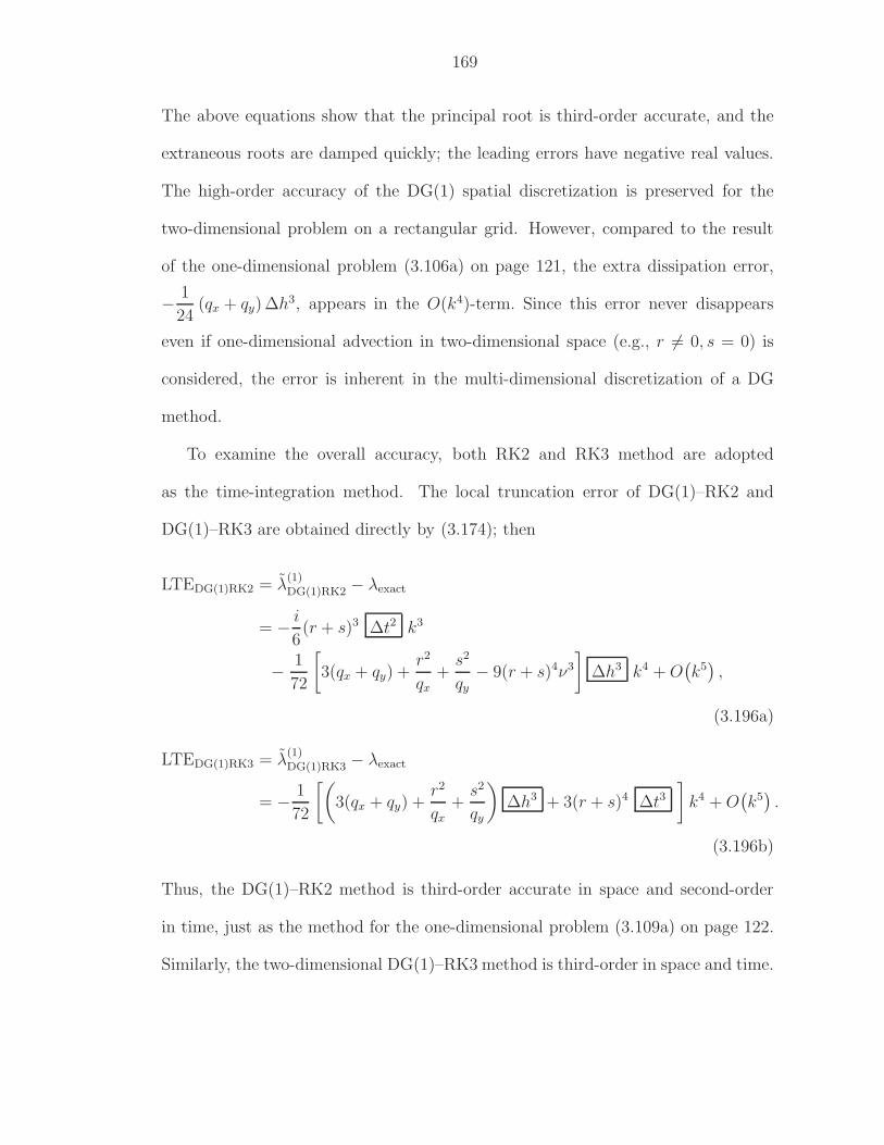
169
The above equations show that the principal root is third-order accurate, and the
extraneous roots are damped quickly; the leading errors have negative real values.
The high-order accuracy of the DG(1) spatial discretization is preserved for the
two-dimensional problem on a rectangular grid. However, compared to the result
of the one-dimensional problem (3.106a) on page 121, the extra dissipation error,
− 1
24(qx + qy) ∆h3, appears in the O(k4)-term. Since this error never disappears
even if one-dimensional advection in two-dimensional space (e.g., r 6= 0, s = 0) is
considered, the error is inherent in the multi-dimensional discretization of a DG
method.
To examine the overall accuracy, both RK2 and RK3 method are adopted
as the time-integration method. The local truncation error of DG(1)–RK2 and
DG(1)–RK3 are obtained directly by (3.174); then
LTEDG(1)RK2 = λ(1)DG(1)RK2 − λexact
= − i
6(r + s)3 ∆t2 k3
− 1
72
[3(qx + qy) +
r2
qx+
s2
qy− 9(r + s)4ν3
]∆h3 k4 + O
(k5),
(3.196a)
LTEDG(1)RK3 = λ(1)DG(1)RK3 − λexact
= − 1
72
[(3(qx + qy) +
r2
qx+
s2
qy
)∆h3 + 3(r + s)4 ∆t3
]k4 + O
(k5).
(3.196b)
Thus, the DG(1)–RK2 method is third-order accurate in space and second-order
in time, just as the method for the one-dimensional problem (3.109a) on page 122.
Similarly, the two-dimensional DG(1)–RK3 method is third-order in space and time.
170
Stability The modulus of the amplification factors of both DG(1)–RK2 and
DG(1)–RK3 methods with the upwind flux are shown in Figure 3.19. Based on the
numerical contour plots of the modulus, the stability condition of each method in
terms of ν2D is
νupwind2D, DG(1)RK2 = νx + νy ≤ 0.333, (3.197a)
νupwind2D, DG(1)RK3 = νx + νy ≤ 0.409, (3.197b)
respectively. Thus, adding another stage slightly increases the stability domain, and
also the order of accuracy. A drawback is that the RK3 requires an extra Riemann
solver to compute at each cell interface.
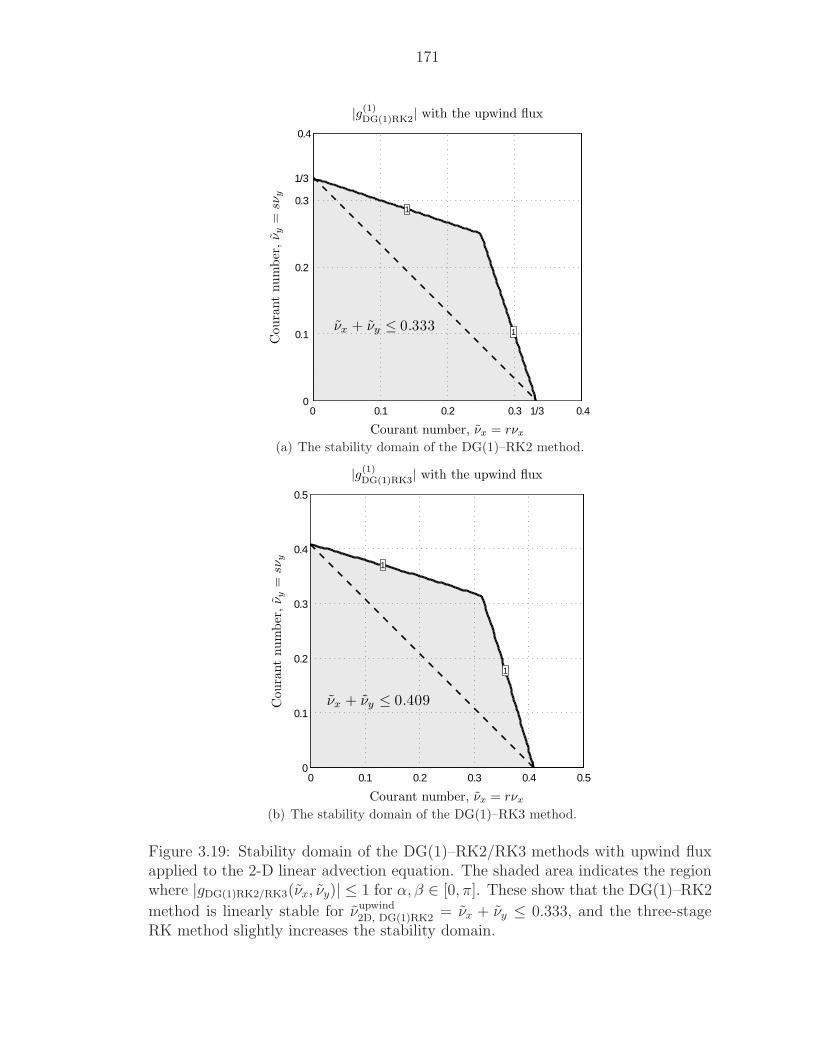
171
0 0.1 0.2 0.3 1/3 0.40
0.1
0.2
0.3
1/3
0.4
1
1
νx + νy ≤ 0.333
Courant number, νx = rνx
Coura
nt
num
ber
,ν y
=sν
y
|g(1)DG(1)RK2| with the upwind flux
(a) The stability domain of the DG(1)–RK2 method.
0 0.1 0.2 0.3 0.4 0.50
0.1
0.2
0.3
0.4
0.5
1
1
νx + νy ≤ 0.409
Courant number, νx = rνx
Coura
nt
num
ber
,ν y
=sν
y
|g(1)DG(1)RK3| with the upwind flux
(b) The stability domain of the DG(1)–RK3 method.
Figure 3.19: Stability domain of the DG(1)–RK2/RK3 methods with upwind fluxapplied to the 2-D linear advection equation. The shaded area indicates the regionwhere |gDG(1)RK2/RK3(νx, νy)| ≤ 1 for α, β ∈ [0, π]. These show that the DG(1)–RK2
method is linearly stable for νupwind2D, DG(1)RK2 = νx + νy ≤ 0.333, and the three-stage
RK method slightly increases the stability domain.
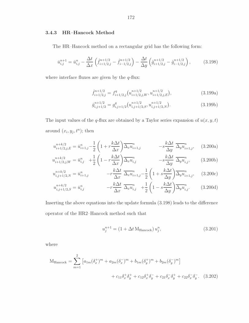
172
3.4.3 HR–Hancock Method
The HR–Hancock method on a rectangular grid has the following form:
un+1i,j = un
i,j −∆t
∆x
(f
n+1/2i+1/2,j − f
n+1/2i−1/2,j
)− ∆t
∆y
(g
n+1/2i+1/2,j − g
n+1/2i−1/2,j
), (3.198)
where interface fluxes are given by the q-flux:
fn+1/2i+1/2,j = f q
i+1/2,j
(u
n+1/2i+1/2,j,W , u
n+1/2i+1/2,j,E
), (3.199a)
gn+1/2i,j+1/2 = gq
i,j+1/2
(u
n+1/2i,j+1/2,S, u
n+1/2i,j+1/2,N
). (3.199b)
The input values of the q-flux are obtained by a Taylor series expansion of u(x, y, t)
around (xi, yj, tn); then
un+k/2i+1/2,j,E = un
i+1,j−1
2
(1 + r
k∆t
∆x
)∆xu
n
i+1,j −sk∆t
∆y∆yu
n
i+1,j, (3.200a)
un+k/2i+1/2,j,W = un
i,j +1
2
(1 − r
k∆t
∆x
)∆xu
n
i,j −sk∆t
∆y∆yu
n
i,j, (3.200b)
un+k/2i,j+1/2,N = un
i+1,j −rk∆t
∆x∆xu
n
i+1,j−1
2
(1 + s
k∆t
∆y
)∆yu
n
i+1,j, (3.200c)
un+k/2i,j+1/2,S = un
i,j −rk∆t
∆x∆xu
n
i,j +1
2
(1 − s
k∆t
∆y
)∆yu
n
i,j. (3.200d)
Inserting the above equations into the update formula (3.198) leads to the difference
operator of the HR2–Hancock method such that
un+1j = (1 + ∆t MHancock) un
j , (3.201)
where
MHancock =
2∑
m=1
[a1m(δ+
x )m + a2m(δ−x )m + b1m(δ+y )m + b2m(δ−y )m
]
+ c11δ+x δ+
y + c12δ+x δ−y + c21δ
−x δ+
y + c22δ−x δ−y . (3.202)
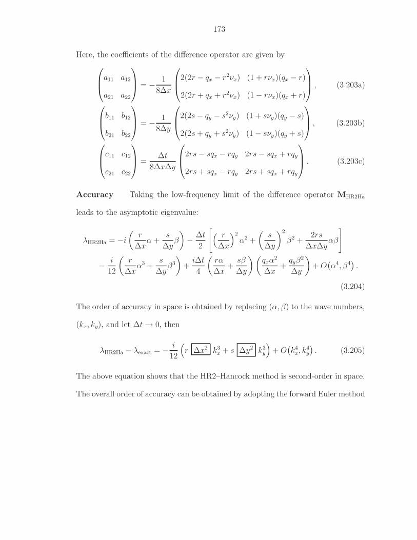
173
Here, the coefficients of the difference operator are given by
a11 a12
a21 a22
= − 1
8∆x
2(2r − qx − r2νx) (1 + rνx)(qx − r)
2(2r + qx + r2νx) (1 − rνx)(qx + r)
, (3.203a)
b11 b12
b21 b22
= − 1
8∆y
2(2s − qy − s2νy) (1 + sνy)(qy − s)
2(2s + qy + s2νy) (1 − sνy)(qy + s)
, (3.203b)
c11 c12
c21 c22
=
∆t
8∆x∆y
2rs − sqx − rqy 2rs − sqx + rqy
2rs + sqx − rqy 2rs + sqx + rqy
. (3.203c)
Accuracy Taking the low-frequency limit of the difference operator MHR2Ha
leads to the asymptotic eigenvalue:
λHR2Ha = −i
(r
∆xα +
s
∆yβ
)− ∆t
2
[( r
∆x
)2
α2 +
(s
∆y
)2
β2 +2rs
∆x∆yαβ
]
− i
12
(r
∆xα3 +
s
∆yβ3
)+
i∆t
4
(rα
∆x+
sβ
∆y
)(qxα
2
∆x+
qyβ2
∆y
)+ O
(α4, β4
).
(3.204)
The order of accuracy in space is obtained by replacing (α, β) to the wave numbers,
(kx, ky), and let ∆t → 0, then
λHR2Ha − λexact = − i
12
(r ∆x2 k3
x + s ∆y2 k3y
)+ O
(k4
x, k4y
). (3.205)
The above equation shows that the HR2–Hancock method is second-order in space.
The overall order of accuracy can be obtained by adopting the forward Euler method
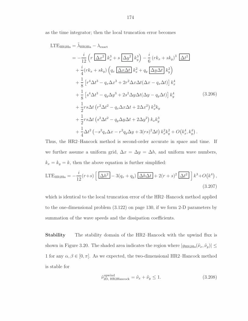
174
as the time integrator; then the local truncation error becomes
LTEHR2Ha = λHR2Ha − λexact
= − i
12
(r ∆x2 k3
x + s ∆y2 k3y
)− i
6(rkx + sky)
3 ∆t2
+i
4(rkx + sky)
(qx ∆x∆t k2
x + qy ∆y∆t k2y
)
+1
8
[r4∆t3 − qx∆x3 + 2r2∆x∆t(∆x − qx∆t)
]k4
x
+1
8
[s4∆t3 − qy∆y3 + 2s2∆y∆t(∆y − qy∆t)
]k4
y
+1
2rs∆t
(r2∆t2 − qx∆x∆t + 2∆x2
)k3
xky
+1
2rs∆t
(s2∆t2 − qy∆y∆t + 2∆y2
)kxk
3y
+1
4∆t2
(−s2qx∆x − r2qy∆y + 3(rs)2∆t
)k2
xk2y + O
(k4
x, k4y
).
(3.206)
Thus, the HR2–Hancock method is second-order accurate in space and time. If
we further assume a uniform grid, ∆x = ∆y = ∆h, and uniform wave numbers,
kx = ky = k, then the above equation is further simplified:
LTEHR2Ha = − i
12(r+s)
[∆h2 − 3(qx + qy) ∆h∆t + 2(r + s)2 ∆t2
]k3+O
(k4),
(3.207)
which is identical to the local truncation error of the HR2–Hancock method applied
to the one-dimensional problem (3.122) on page 130, if we form 2-D parameters by
summation of the wave speeds and the dissipation coefficients.
Stability The stability domain of the HR2–Hancock with the upwind flux is
shown in Figure 3.20. The shaded area indicates the region where |gHR2Ha(νx, νy)| ≤
1 for any α, β ∈ [0, π]. As we expected, the two-dimensional HR2–Hancock method
is stable for
νupwind2D, HR2Hancock = νx + νy ≤ 1. (3.208)
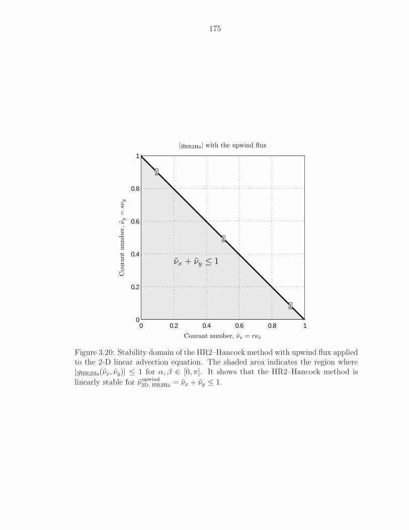
175
0 0.2 0.4 0.6 0.8 10
0.2
0.4
0.6
0.8
1
1
1
1
νx + νy ≤ 1
Courant number, νx = rνx
Coura
nt
num
ber
,ν y
=sν
y
|gHR2Ha| with the upwind flux
Figure 3.20: Stability domain of the HR2–Hancock method with upwind flux appliedto the 2-D linear advection equation. The shaded area indicates the region where|gHR2Ha(νx, νy)| ≤ 1 for α, β ∈ [0, π]. It shows that the HR2–Hancock method is
linearly stable for νupwind2D, HR2Ha = νx + νy ≤ 1.
176
3.4.4 DG–Hancock Method
The DG(1)–Hancock method on a rectangular grid has the following update
formulas:
un+1i,j = un
i,j −∆t
∆x
(f
n+1/2i+1/2,j − f
n+1/2i−1/2,j
)− ∆t
∆y
(g
n+1/2i+1/2,j − g
n+1/2i−1/2,j
), (3.209a)
∆xun+1
i,j = ∆xun
i,j −∆t
∆x6(f
n+1/2i+1/2,j + f
n+1/2i−1/2,j − 2rui,j
)
− ∆t
∆y12
1∫
0
(ξ − 1
2
)g
n+1/2ξ,j+1/2(ξ) dξ −
1∫
0
(ξ − 1
2
)g
n+1/2ξ,j−1/2(ξ) dξ
,
(3.209b)
∆yun+1
i,j = ∆yun
i,j −∆t
∆y6(g
n+1/2i,j+1/2 + g
n+1/2i,j−1/2 − 2sui,j
)
− ∆t
∆x12
1∫
0
(η − 1
2
)f
n+1/2i+1/2,η(η) dη −
1∫
0
(η − 1
2
)f
n+1/2i−1/2,η(η) dη
,
(3.209c)
where the fluxes in both coordinate directions are given by the q-flux (3.199). The
volume integral of the flux simplifies owing to flux linearity, and quadrature is only
required in time. Again, both Gauss–Lobatto and Gauss–Radau quadratures in
time:
3-point Gauss–Lobatto
uj =1
6(un
j + 4un+1/2j + un+1
j ), (3.210)
where
un+1/2j = un
j − ∆t
2
1
∆x
(f
n+1/4j+1/2 − f
n+1/4j−1/2
), (3.211)
2-point Gauss–Radau
uj =1
4(3u
n+1/3j + un+1
j ), (3.212)
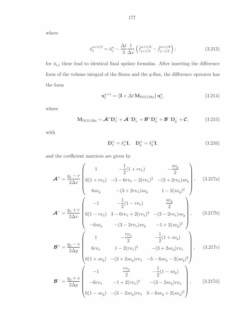
177
where
un+1/3j = un
j − ∆t
3
1
∆x
(f
n+1/6j+1/2 − f
n+1/6j−1/2
); (3.213)
for ui,j these lead to identical final update formulas. After inserting the difference
form of the volume integral of the fluxes and the q-flux, the difference operator has
the form
un+1j =
(I + ∆tMDG(1)Ha
)un
j , (3.214)
where
MDG(1)Ha = A+D+
x + A−D−
x + B+D+
y + B−D−
y + C, (3.215)
with
D±x = δ±x I, D±
y = δ±y I, (3.216)
and the coefficient matrices are given by
A+ =
qx − r
2∆x
1 −1
2(1 + rνx) −sνy
2
6(1 + rνx) −3 − 6rνx − 2(rνx)2 −(3 + 2rνx)sνy
6sνy −(3 + 2rνx)sνy 1 − 2(sνy)2
, (3.217a)
A− =
qx + r
2∆x
−1 −1
2(1 − rνx)
sνy
2
6(1 − rνx) 3 − 6rνx + 2(rνx)2 −(3 − 2rνx)sνy
−6sνy −(3 − 2rνx)sνy −1 + 2(sνy)2
, (3.217b)
B+ =
qy − s
2∆y
1 −rνx
2−1
2(1 + sνy)
6rνx 1 − 2(rνx)2 −(3 + 2sνy)rνx
6(1 + sνy) −(3 + 2sνy)rνx −3 − 6sνy − 2(sνy)2
, (3.217c)
B− =
qy + s
2∆y
−1rνx
2−1
2(1 − sνy)
−6rνx −1 + 2(rνx)2 −(3 − 2sνy)rνx
6(1 − sνy) −(3 − 2sνy)rνx 3 − 6sνy + 2(sνy)2
, (3.217d)
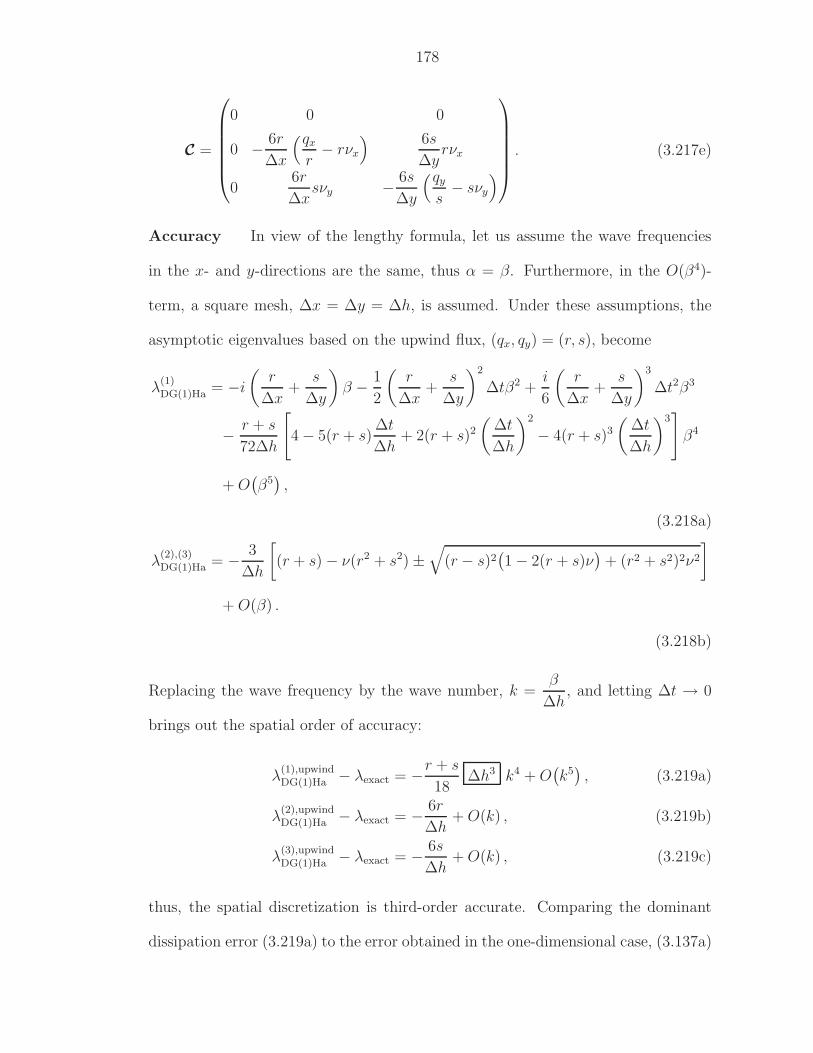
178
C =
0 0 0
0 − 6r
∆x
(qx
r− rνx
) 6s
∆yrνx
06r
∆xsνy − 6s
∆y
(qy
s− sνy
)
. (3.217e)
Accuracy In view of the lengthy formula, let us assume the wave frequencies
in the x- and y-directions are the same, thus α = β. Furthermore, in the O(β4)-
term, a square mesh, ∆x = ∆y = ∆h, is assumed. Under these assumptions, the
asymptotic eigenvalues based on the upwind flux, (qx, qy) = (r, s), become
λ(1)DG(1)Ha = −i
(r
∆x+
s
∆y
)β − 1
2
(r
∆x+
s
∆y
)2
∆tβ2 +i
6
(r
∆x+
s
∆y
)3
∆t2β3
− r + s
72∆h
[4 − 5(r + s)
∆t
∆h+ 2(r + s)2
(∆t
∆h
)2
− 4(r + s)3
(∆t
∆h
)3]
β4
+ O(β5),
(3.218a)
λ(2),(3)DG(1)Ha = − 3
∆h
[(r + s) − ν(r2 + s2) ±
√(r − s)2
(1 − 2(r + s)ν
)+ (r2 + s2)2ν2
]
+ O(β) .
(3.218b)
Replacing the wave frequency by the wave number, k =β
∆h, and letting ∆t → 0
brings out the spatial order of accuracy:
λ(1),upwindDG(1)Ha − λexact = −r + s
18∆h3 k4 + O
(k5), (3.219a)
λ(2),upwindDG(1)Ha − λexact = − 6r
∆h+ O(k) , (3.219b)
λ(3),upwindDG(1)Ha − λexact = − 6s
∆h+ O(k) , (3.219c)
thus, the spatial discretization is third-order accurate. Comparing the dominant
dissipation error (3.219a) to the error obtained in the one-dimensional case, (3.137a)
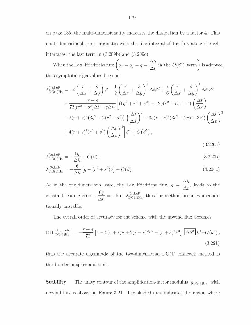
179
on page 135, the multi-dimensionality increases the dissipation by a factor 4. This
multi-dimensional error originates with the line integral of the flux along the cell
interfaces, the last term in (3.209b) and (3.209c).
When the Lax–Friedrichs flux
(qx = qy = q =
∆h
∆tin the O(β4) term
)is adopted,
the asymptotic eigenvalues become
λ(1),LxFDG(1)Ha = −i
(r
∆x+
s
∆y
)β − 1
2
(r
∆x+
s
∆y
)2
∆tβ2 +i
6
(r
∆x+
s
∆y
)3
∆t2β3
− r + s
72[(r2 + s2)∆t − q∆h]
[(6q2 + r2 + s2) − 12q(r2 + rs + s2)
(∆t
∆x
)
+ 2(r + s)2(3q2 + 2(r2 + s2)
)(∆t
∆x
)2
− 3q(r + s)2(3r2 + 2rs + 3s2)
(∆t
∆x
)3
+ 4(r + s)4(r2 + s2)
(∆t
∆x
)4]β4 + O
(β5),
(3.220a)
λ(2),LxFDG(1)Ha = − 6q
∆h+ O(β) , (3.220b)
λ(3),LxFDG(1)Ha = − 6
∆h
[q − (r2 + s2)ν
]+ O(β) . (3.220c)
As in the one-dimensional case, the Lax–Friedrichs flux, q =∆h
∆t, leads to the
constant leading error − 6q
∆h= −6 in λ
(2),LxFDG(1)Ha, thus the method becomes uncondi-
tionally unstable.
The overall order of accuracy for the scheme with the upwind flux becomes
LTE(1),upwindDG(1)Ha = −r + s
72
[4 − 5(r + s)ν + 2(r + s)2ν2 − (r + s)3ν3
]∆h3 k4+O
(k5),
(3.221)
thus the accurate eigenmode of the two-dimensional DG(1)–Hancock method is
third-order in space and time.
Stability The unity contour of the amplification-factor modulus |gDG(1)Ha| with
upwind flux is shown in Figure 3.21. The shaded area indicates the region where
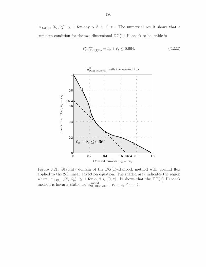
180
|gDG(1)Ha(νx, νy)| ≤ 1 for any α, β ∈ [0, π]. The numerical result shows that a
sufficient condition for the two-dimensional DG(1)–Hancock to be stable is
νupwind2D, DG(1)Ha = νx + νy ≤ 0.664. (3.222)
0 0.2 0.4 0.6 0.664 0.8 1.00
0.2
0.4
0.6
0.664
0.8
1
1
1
νx + νy ≤ 0.664
Courant number, νx = rνx
Coura
nt
num
ber
,ν y
=sν
y
|g(1)DG(1)Hancock| with the upwind flux
Figure 3.21: Stability domain of the DG(1)–Hancock method with upwind fluxapplied to the 2-D linear advection equation. The shaded area indicates the regionwhere |gDG(1)Ha(νx, νy)| ≤ 1 for α, β ∈ [0, π]. It shows that the DG(1)–Hancock
method is linearly stable for νupwind2D, DG(1)Ha = νx + νy ≤ 0.664.
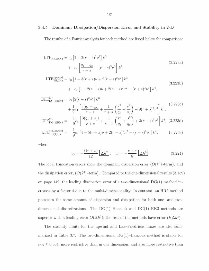
181
3.4.5 Dominant Dissipation/Dispersion Error and Stability in 2-D
The results of a Fourier analysis for each method are listed below for comparison:
LTEHR2RK2 = c3
[1 + 2(r + s)2ν2
]k3
+ c4
[qx + qy
r + s− (r + s)3ν3
]k4,
(3.223a)
LTEupwindHR2Ha = c3
[1 − 3(r + s)ν + 2(r + s)2ν2
]k3
+ c4
[1 − 2(r + s)ν + 2(r + s)2ν2 − (r + s)3ν3
]k4,
(3.223b)
LTE(1)DG(1)RK2 = c3
[2(r + s)2ν2
]k3
+1
9c4
[3(qx + qy)
r + s+
1
r + s
(r2
qx+
s2
qy
)− 9(r + s)3ν3
]k4,
(3.223c)
LTE(1)DG(1)RK3 =
1
9c4
[3(qx + qy)
r + s+
1
r + s
(r2
qx+
s2
qy
)+ 3(r + s)3ν3
]k4, (3.223d)
LTE(1),upwindDG(1)Ha =
1
9c4
[4 − 5(r + s)ν + 2(r + s)2ν2 − (r + s)3ν3
]k4, (3.223e)
where
c3 = −i (r + s)
12∆h2 , c4 = −r + s
8∆h3 . (3.224)
The local truncation errors show the dominant dispersion error(O(k3) -term
), and
the dissipation error,(O(k4) -term
). Compared to the one-dimensional results (3.159)
on page 149, the leading dissipation error of a two-dimensional DG(1) method in-
creases by a factor 4 due to the multi-dimensionality. In contrast, an HR2 method
possesses the same amount of dispersion and dissipation for both one- and two-
dimensional discretizations. The DG(1)–Hancock and DG(1)–RK3 methods are
superior with a leading error O(∆h3); the rest of the methods have error O(∆h2).
The stability limits for the upwind and Lax–Friedrichs fluxes are also sum-
marized in Table 3.7. The two-dimensional DG(1)–Hancock method is stable for
ν2D ≤ 0.664, more restrictive than in one dimension, and also more restrictive than
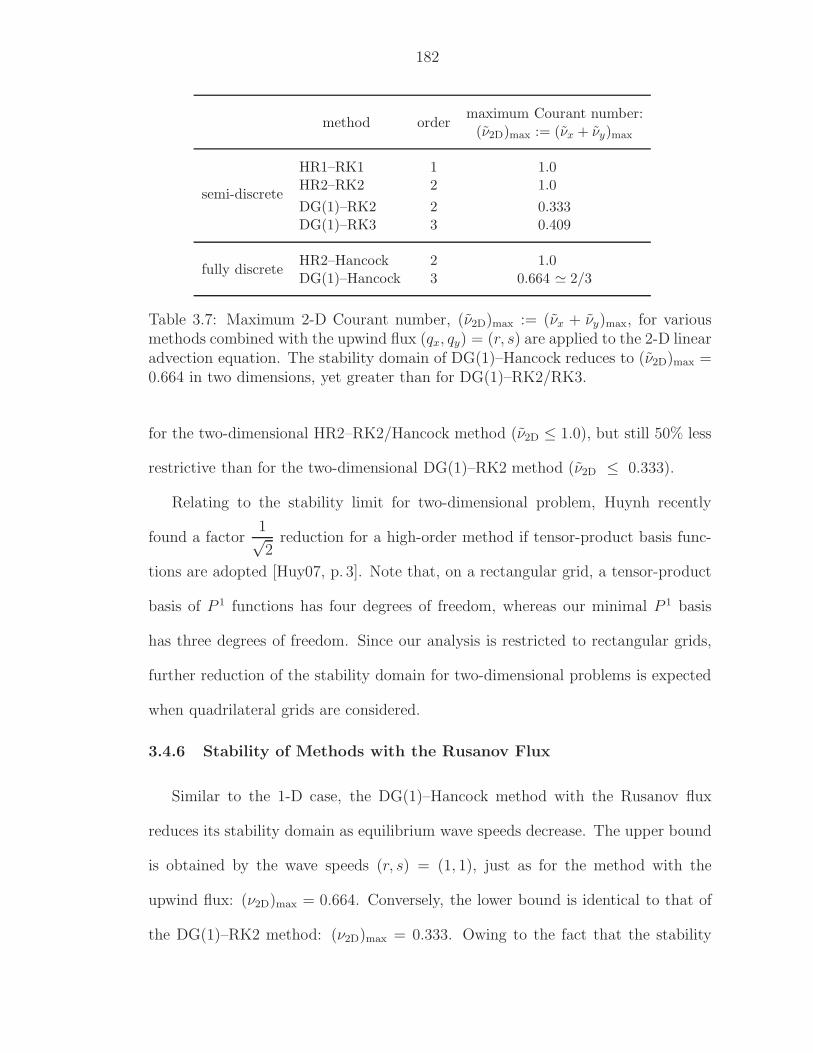
182
method ordermaximum Courant number:
(ν2D)max := (νx + νy)max
semi-discrete
HR1–RK1 1 1.0HR2–RK2 2 1.0
DG(1)–RK2 2 0.333DG(1)–RK3 3 0.409
fully discreteHR2–Hancock 2 1.0DG(1)–Hancock 3 0.664 ≃ 2/3
Table 3.7: Maximum 2-D Courant number, (ν2D)max := (νx + νy)max, for variousmethods combined with the upwind flux (qx, qy) = (r, s) are applied to the 2-D linearadvection equation. The stability domain of DG(1)–Hancock reduces to (ν2D)max =0.664 in two dimensions, yet greater than for DG(1)–RK2/RK3.
for the two-dimensional HR2–RK2/Hancock method (ν2D ≤ 1.0), but still 50% less
restrictive than for the two-dimensional DG(1)–RK2 method (ν2D ≤ 0.333).
Relating to the stability limit for two-dimensional problem, Huynh recently
found a factor1√2
reduction for a high-order method if tensor-product basis func-
tions are adopted [Huy07, p. 3]. Note that, on a rectangular grid, a tensor-product
basis of P 1 functions has four degrees of freedom, whereas our minimal P 1 basis
has three degrees of freedom. Since our analysis is restricted to rectangular grids,
further reduction of the stability domain for two-dimensional problems is expected
when quadrilateral grids are considered.
3.4.6 Stability of Methods with the Rusanov Flux
Similar to the 1-D case, the DG(1)–Hancock method with the Rusanov flux
reduces its stability domain as equilibrium wave speeds decrease. The upper bound
is obtained by the wave speeds (r, s) = (1, 1), just as for the method with the
upwind flux: (ν2D)max = 0.664. Conversely, the lower bound is identical to that of
the DG(1)–RK2 method: (ν2D)max = 0.333. Owing to the fact that the stability
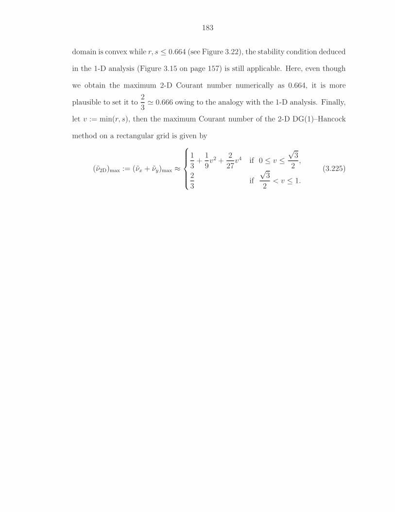
183
domain is convex while r, s ≤ 0.664 (see Figure 3.22), the stability condition deduced
in the 1-D analysis (Figure 3.15 on page 157) is still applicable. Here, even though
we obtain the maximum 2-D Courant number numerically as 0.664, it is more
plausible to set it to2
3≃ 0.666 owing to the analogy with the 1-D analysis. Finally,
let v := min(r, s), then the maximum Courant number of the 2-D DG(1)–Hancock
method on a rectangular grid is given by
(ν2D)max := (νx + νy)max ≈
1
3+
1
9v2 +
2
27v4 if 0 ≤ v ≤
√3
2,
2
3if
√3
2< v ≤ 1.
(3.225)
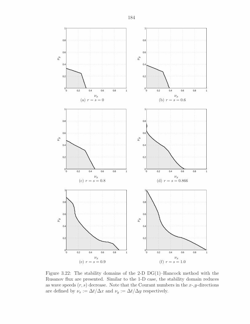
184
0 0.2 0.4 0.6 0.8 10
0.2
0.4
0.6
0.8
1
νx
ν y
(a) r = s = 0
0 0.2 0.4 0.6 0.8 10
0.2
0.4
0.6
0.8
1
νx
ν y
(b) r = s = 0.6
0 0.2 0.4 0.6 0.8 10
0.2
0.4
0.6
0.8
1
νx
ν y
(c) r = s = 0.8
0 0.2 0.4 0.6 0.8 10
0.2
0.4
0.6
0.8
1
νx
ν y
(d) r = s = 0.866
0 0.2 0.4 0.6 0.8 10
0.2
0.4
0.6
0.8
1
νx
ν y
(e) r = s = 0.9
0 0.2 0.4 0.6 0.8 10
0.2
0.4
0.6
0.8
1
νx
ν y
(f) r = s = 1.0
Figure 3.22: The stability domains of the 2-D DG(1)–Hancock method with theRusanov flux are presented. Similar to the 1-D case, the stability domain reducesas wave speeds (r, s) decrease. Note that the Courant numbers in the x-,y-directionsare defined by νx := ∆t/∆x and νy := ∆t/∆y respectively.
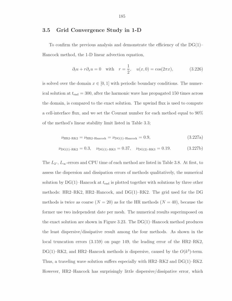
185
3.5 Grid Convergence Study in 1-D
To confirm the previous analysis and demonstrate the efficiency of the DG(1)–
Hancock method, the 1-D linear advection equation,
∂tu + r∂xu = 0 with r =1
2, u(x, 0) = cos(2πx), (3.226)
is solved over the domain x ∈ [0, 1] with periodic boundary conditions. The numer-
ical solution at tend = 300, after the harmonic wave has propagated 150 times across
the domain, is compared to the exact solution. The upwind flux is used to compute
a cell-interface flux, and we set the Courant number for each method equal to 90%
of the method’s linear stability limit listed in Table 3.3;
νHR2–RK2 = νHR2–Hancock = νDG(1)–Hancock = 0.9, (3.227a)
νDG(1)–RK2 = 0.3, νDG(1)–RK3 = 0.37, νDG(2)–RK3 = 0.19. (3.227b)
The L2-, L∞-errors and CPU time of each method are listed in Table 3.8. At first, to
assess the dispersion and dissipation errors of methods qualitatively, the numerical
solution by DG(1)–Hancock at tend is plotted together with solutions by three other
methods: HR2–RK2, HR2–Hancock, and DG(1)–RK2. The grid used for the DG
methods is twice as coarse (N = 20) as for the HR methods (N = 40), because the
former use two independent date per mesh. The numerical results superimposed on
the exact solution are shown in Figure 3.23. The DG(1)–Hancock method produces
the least dispersive/dissipative result among the four methods. As shown in the
local truncation errors (3.159) on page 149, the leading error of the HR2–RK2,
DG(1)–RK2, and HR2–Hancock methods is dispersive, caused by the O(k3)-term.
Thus, a traveling wave solution suffers especially with HR2–RK2 and DG(1)–RK2.
However, HR2–Hancock has surprisingly little dispersive/dissipative error, which
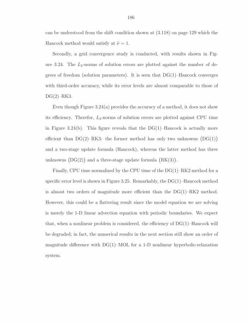
186
can be understood from the shift condition shown at (3.118) on page 129 which the
Hancock method would satisfy at ν = 1.
Secondly, a grid convergence study is conducted, with results shown in Fig-
ure 3.24. The L2-norms of solution errors are plotted against the number of de-
grees of freedom (solution parameters). It is seen that DG(1)–Hancock converges
with third-order accuracy, while its error levels are almost comparable to those of
DG(2)–RK3.
Even though Figure 3.24(a) provides the accuracy of a method, it does not show
its efficiency. Therefor, L2-norms of solution errors are plotted against CPU time
in Figure 3.24(b). This figure reveals that the DG(1)–Hancock is actually more
efficient than DG(2)–RK3: the former method has only two unknowns(DG(1)
)
and a two-stage update formula (Hancock), whereas the latter method has three
unknowns(DG(2)
)and a three-stage update formula
(RK(3)
).
Finally, CPU time normalized by the CPU time of the DG(1)–RK2 method for a
specific error level is shown in Figure 3.25. Remarkably, the DG(1)–Hancock method
is almost two orders of magnitude more efficient than the DG(1)–RK2 method.
However, this could be a flattering result since the model equation we are solving
is merely the 1-D linear advection equation with periodic boundaries. We expect
that, when a nonlinear problem is considered, the efficiency of DG(1)–Hancock will
be degraded; in fact, the numerical results in the next section still show an order of
magnitude difference with DG(1)–MOL for a 1-D nonlinear hyperbolic-relaxation
system.
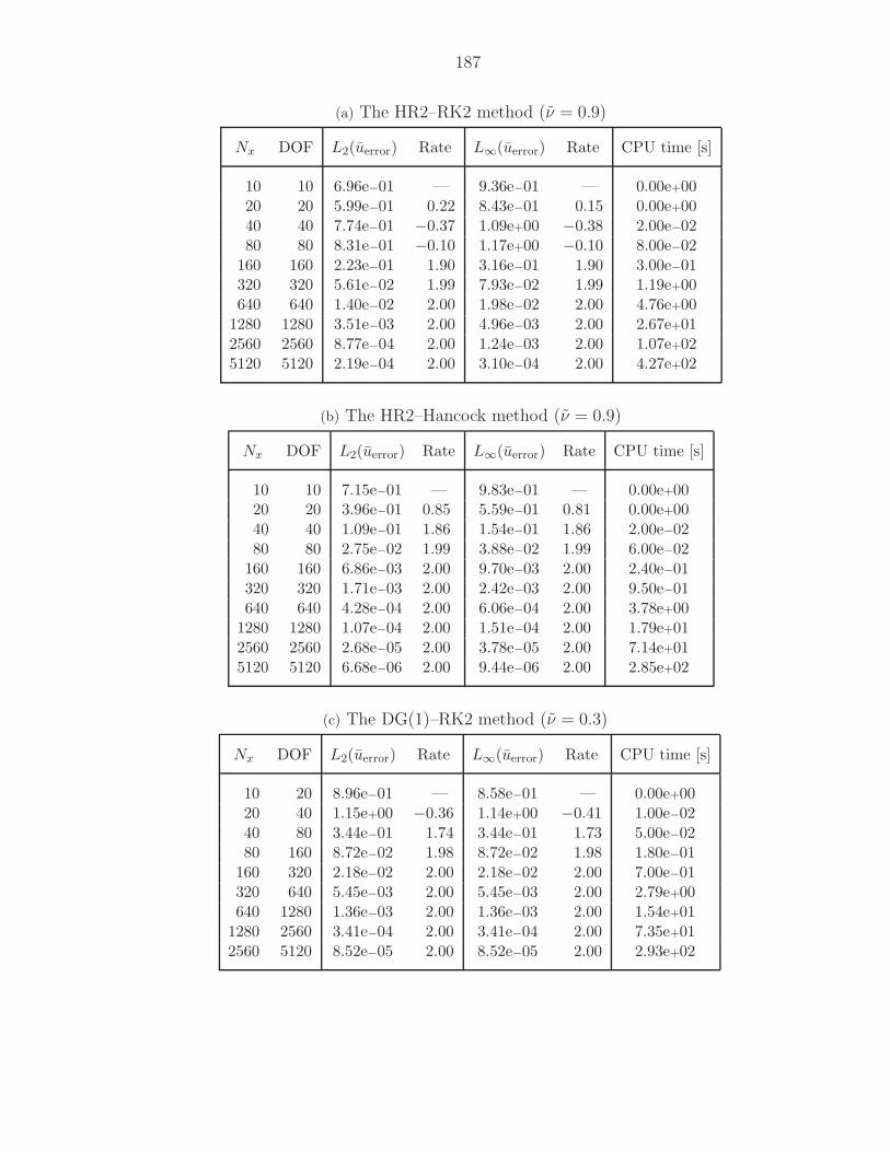
187
(a) The HR2–RK2 method (ν = 0.9)
Nx DOF L2(uerror) Rate L∞(uerror) Rate CPU time [s]
10 10 6.96e−01 — 9.36e−01 — 0.00e+0020 20 5.99e−01 0.22 8.43e−01 0.15 0.00e+0040 40 7.74e−01 −0.37 1.09e+00 −0.38 2.00e−0280 80 8.31e−01 −0.10 1.17e+00 −0.10 8.00e−02
160 160 2.23e−01 1.90 3.16e−01 1.90 3.00e−01320 320 5.61e−02 1.99 7.93e−02 1.99 1.19e+00640 640 1.40e−02 2.00 1.98e−02 2.00 4.76e+00
1280 1280 3.51e−03 2.00 4.96e−03 2.00 2.67e+012560 2560 8.77e−04 2.00 1.24e−03 2.00 1.07e+025120 5120 2.19e−04 2.00 3.10e−04 2.00 4.27e+02
(b) The HR2–Hancock method (ν = 0.9)
Nx DOF L2(uerror) Rate L∞(uerror) Rate CPU time [s]
10 10 7.15e−01 — 9.83e−01 — 0.00e+0020 20 3.96e−01 0.85 5.59e−01 0.81 0.00e+0040 40 1.09e−01 1.86 1.54e−01 1.86 2.00e−0280 80 2.75e−02 1.99 3.88e−02 1.99 6.00e−02
160 160 6.86e−03 2.00 9.70e−03 2.00 2.40e−01320 320 1.71e−03 2.00 2.42e−03 2.00 9.50e−01640 640 4.28e−04 2.00 6.06e−04 2.00 3.78e+00
1280 1280 1.07e−04 2.00 1.51e−04 2.00 1.79e+012560 2560 2.68e−05 2.00 3.78e−05 2.00 7.14e+015120 5120 6.68e−06 2.00 9.44e−06 2.00 2.85e+02
(c) The DG(1)–RK2 method (ν = 0.3)
Nx DOF L2(uerror) Rate L∞(uerror) Rate CPU time [s]
10 20 8.96e−01 — 8.58e−01 — 0.00e+0020 40 1.15e+00 −0.36 1.14e+00 −0.41 1.00e−0240 80 3.44e−01 1.74 3.44e−01 1.73 5.00e−0280 160 8.72e−02 1.98 8.72e−02 1.98 1.80e−01
160 320 2.18e−02 2.00 2.18e−02 2.00 7.00e−01320 640 5.45e−03 2.00 5.45e−03 2.00 2.79e+00640 1280 1.36e−03 2.00 1.36e−03 2.00 1.54e+01
1280 2560 3.41e−04 2.00 3.41e−04 2.00 7.35e+012560 5120 8.52e−05 2.00 8.52e−05 2.00 2.93e+02
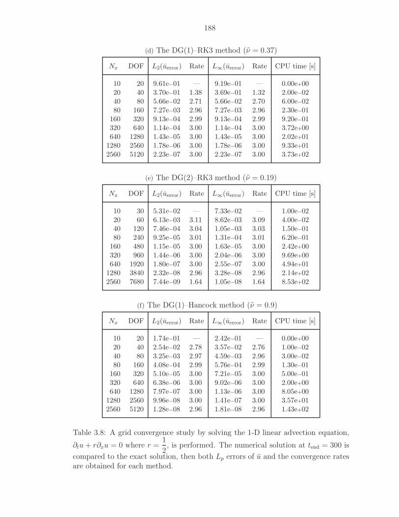
188
(d) The DG(1)–RK3 method (ν = 0.37)
Nx DOF L2(uerror) Rate L∞(uerror) Rate CPU time [s]
10 20 9.61e−01 — 9.19e−01 — 0.00e+0020 40 3.70e−01 1.38 3.69e−01 1.32 2.00e−0240 80 5.66e−02 2.71 5.66e−02 2.70 6.00e−0280 160 7.27e−03 2.96 7.27e−03 2.96 2.30e−01
160 320 9.13e−04 2.99 9.13e−04 2.99 9.20e−01320 640 1.14e−04 3.00 1.14e−04 3.00 3.72e+00640 1280 1.43e−05 3.00 1.43e−05 3.00 2.02e+01
1280 2560 1.78e−06 3.00 1.78e−06 3.00 9.33e+012560 5120 2.23e−07 3.00 2.23e−07 3.00 3.73e+02
(e) The DG(2)–RK3 method (ν = 0.19)
Nx DOF L2(uerror) Rate L∞(uerror) Rate CPU time [s]
10 30 5.31e−02 — 7.33e−02 — 1.00e−0220 60 6.13e−03 3.11 8.62e−03 3.09 4.00e−0240 120 7.46e−04 3.04 1.05e−03 3.03 1.50e−0180 240 9.25e−05 3.01 1.31e−04 3.01 6.20e−01
160 480 1.15e−05 3.00 1.63e−05 3.00 2.42e+00320 960 1.44e−06 3.00 2.04e−06 3.00 9.69e+00640 1920 1.80e−07 3.00 2.55e−07 3.00 4.94e+01
1280 3840 2.32e−08 2.96 3.28e−08 2.96 2.14e+022560 7680 7.44e−09 1.64 1.05e−08 1.64 8.53e+02
(f) The DG(1)–Hancock method (ν = 0.9)
Nx DOF L2(uerror) Rate L∞(uerror) Rate CPU time [s]
10 20 1.74e−01 — 2.42e−01 — 0.00e+0020 40 2.54e−02 2.78 3.57e−02 2.76 1.00e−0240 80 3.25e−03 2.97 4.59e−03 2.96 3.00e−0280 160 4.08e−04 2.99 5.76e−04 2.99 1.30e−01
160 320 5.10e−05 3.00 7.21e−05 3.00 5.00e−01320 640 6.38e−06 3.00 9.02e−06 3.00 2.00e+00640 1280 7.97e−07 3.00 1.13e−06 3.00 8.05e+00
1280 2560 9.96e−08 3.00 1.41e−07 3.00 3.57e+012560 5120 1.28e−08 2.96 1.81e−08 2.96 1.43e+02
Table 3.8: A grid convergence study by solving the 1-D linear advection equation,
∂tu + r∂xu = 0 where r =1
2, is performed. The numerical solution at tend = 300 is
compared to the exact solution, then both Lp errors of u and the convergence ratesare obtained for each method.
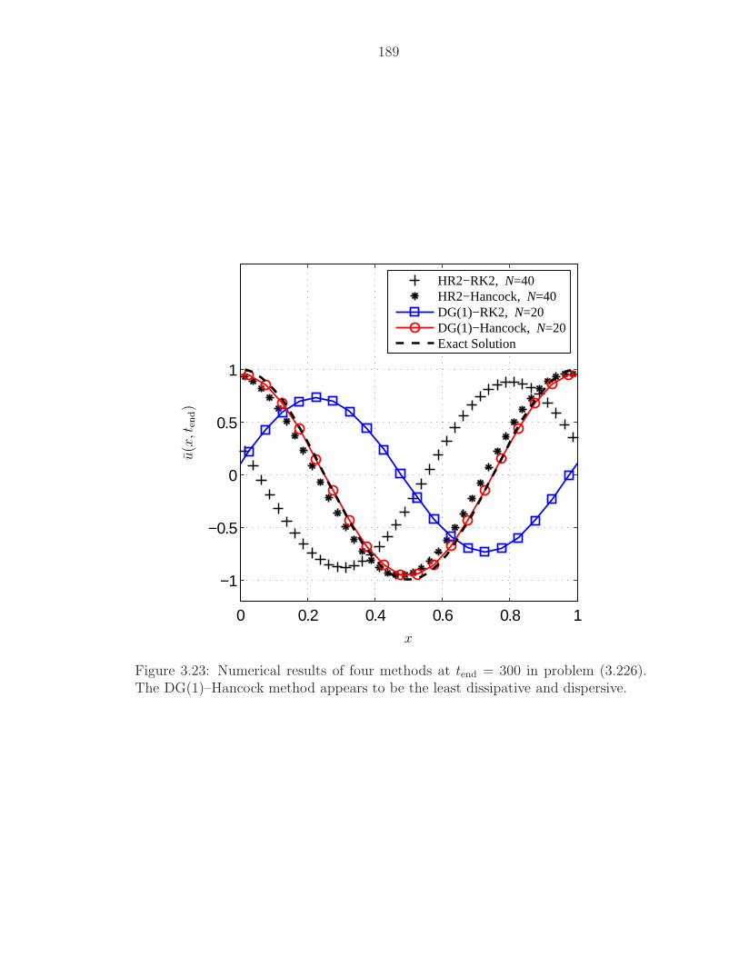
189
0 0.2 0.4 0.6 0.8 1
−1
−0.5
0
0.5
1
HR2−RK2, N=40HR2−Hancock, N=40DG(1)−RK2, N=20DG(1)−Hancock, N=20Exact Solution
x
u(x
,ten
d)
Figure 3.23: Numerical results of four methods at tend = 300 in problem (3.226).The DG(1)–Hancock method appears to be the least dissipative and dispersive.
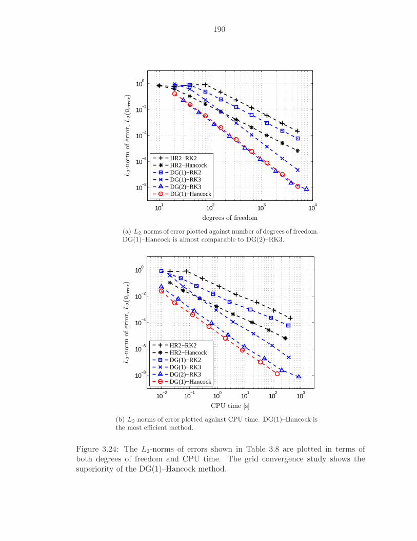
190
101
102
103
104
10−8
10−6
10−4
10−2
100
HR2−RK2HR2−HancockDG(1)−RK2DG(1)−RK3DG(2)−RK3DG(1)−Hancock
degrees of freedom
L2-n
orm
ofer
ror,L
2(u
err
or)
(a) L2-norms of error plotted against number of degrees of freedom.DG(1)–Hancock is almost comparable to DG(2)–RK3.
10−2
10−1
100
101
102
103
10−8
10−6
10−4
10−2
100
HR2−RK2HR2−HancockDG(1)−RK2DG(1)−RK3DG(2)−RK3DG(1)−Hancock
CPU time [s]
L2-n
orm
ofer
ror,L
2(u
err
or)
(b) L2-norms of error plotted against CPU time. DG(1)–Hancock isthe most efficient method.
Figure 3.24: The L2-norms of errors shown in Table 3.8 are plotted in terms ofboth degrees of freedom and CPU time. The grid convergence study shows thesuperiority of the DG(1)–Hancock method.
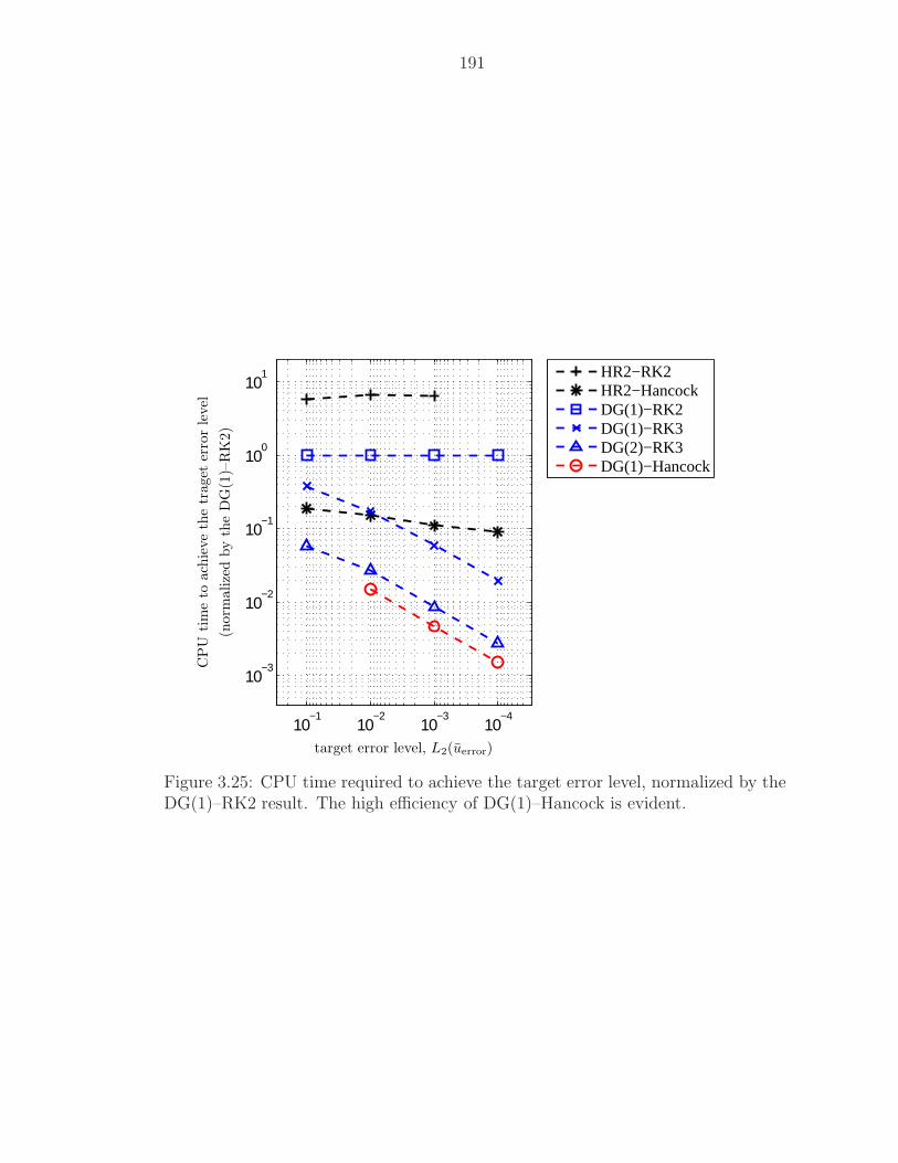
191
10−4
10−3
10−2
10−1
10−3
10−2
10−1
100
101
HR2−RK2HR2−HancockDG(1)−RK2DG(1)−RK3DG(2)−RK3DG(1)−Hancock
target error level, L2(uerror)
CP
Utim
eto
ach
ieve
the
traget
erro
rle
vel
(norm
alize
dby
the
DG
(1)–
RK
2)
Figure 3.25: CPU time required to achieve the target error level, normalized by theDG(1)–RK2 result. The high efficiency of DG(1)–Hancock is evident.
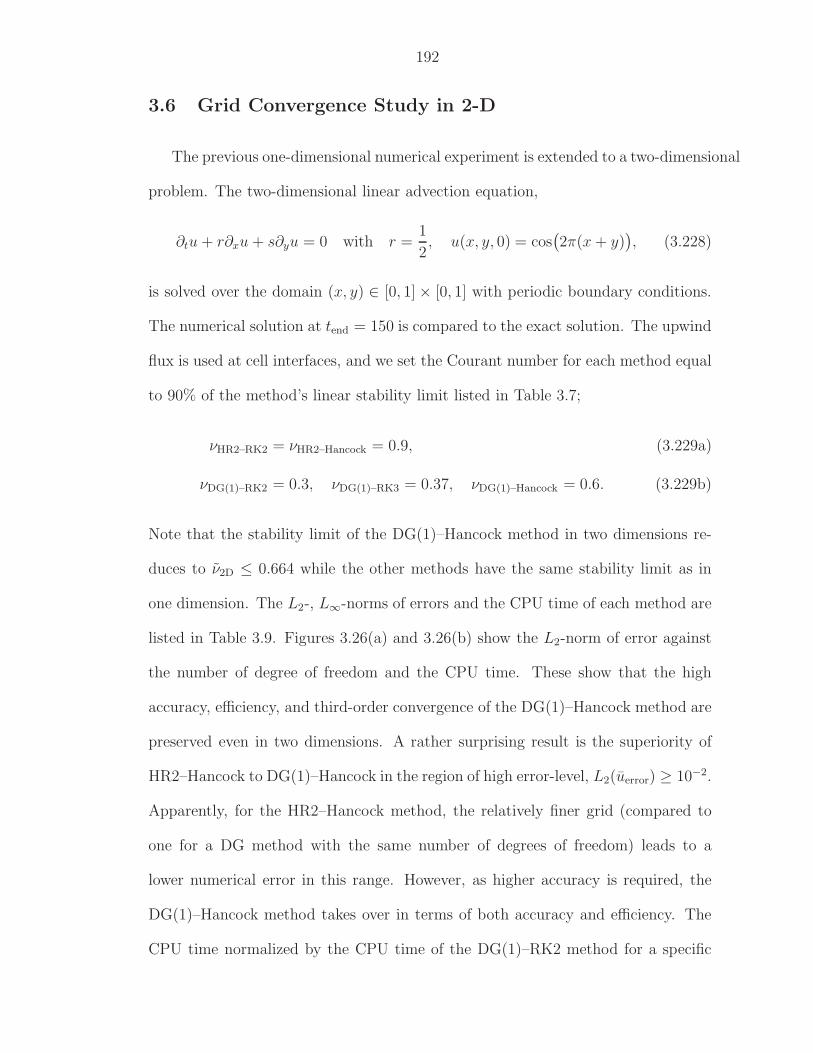
192
3.6 Grid Convergence Study in 2-D
The previous one-dimensional numerical experiment is extended to a two-dimensional
problem. The two-dimensional linear advection equation,
∂tu + r∂xu + s∂yu = 0 with r =1
2, u(x, y, 0) = cos
(2π(x + y)
), (3.228)
is solved over the domain (x, y) ∈ [0, 1] × [0, 1] with periodic boundary conditions.
The numerical solution at tend = 150 is compared to the exact solution. The upwind
flux is used at cell interfaces, and we set the Courant number for each method equal
to 90% of the method’s linear stability limit listed in Table 3.7;
νHR2–RK2 = νHR2–Hancock = 0.9, (3.229a)
νDG(1)–RK2 = 0.3, νDG(1)–RK3 = 0.37, νDG(1)–Hancock = 0.6. (3.229b)
Note that the stability limit of the DG(1)–Hancock method in two dimensions re-
duces to ν2D ≤ 0.664 while the other methods have the same stability limit as in
one dimension. The L2-, L∞-norms of errors and the CPU time of each method are
listed in Table 3.9. Figures 3.26(a) and 3.26(b) show the L2-norm of error against
the number of degree of freedom and the CPU time. These show that the high
accuracy, efficiency, and third-order convergence of the DG(1)–Hancock method are
preserved even in two dimensions. A rather surprising result is the superiority of
HR2–Hancock to DG(1)–Hancock in the region of high error-level, L2(uerror) ≥ 10−2.
Apparently, for the HR2–Hancock method, the relatively finer grid (compared to
one for a DG method with the same number of degrees of freedom) leads to a
lower numerical error in this range. However, as higher accuracy is required, the
DG(1)–Hancock method takes over in terms of both accuracy and efficiency. The
CPU time normalized by the CPU time of the DG(1)–RK2 method for a specific
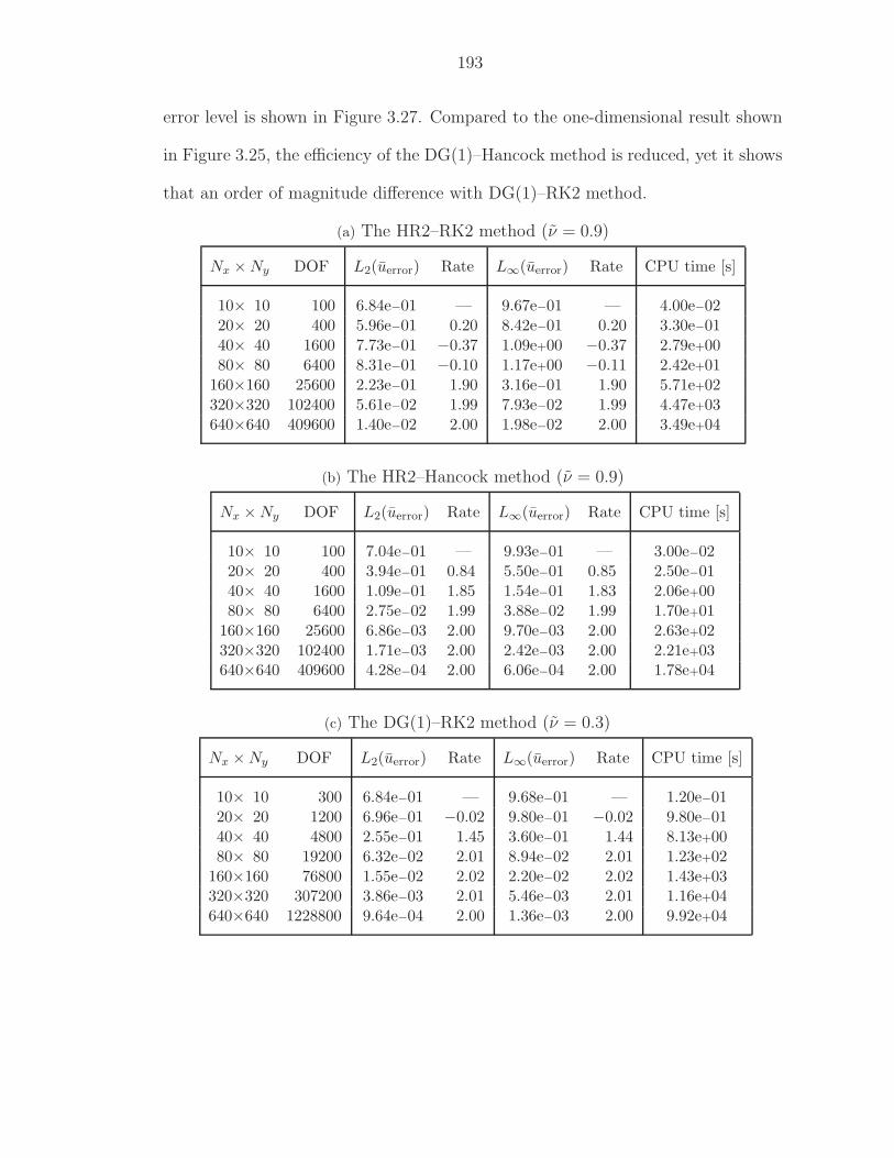
193
error level is shown in Figure 3.27. Compared to the one-dimensional result shown
in Figure 3.25, the efficiency of the DG(1)–Hancock method is reduced, yet it shows
that an order of magnitude difference with DG(1)–RK2 method.
(a) The HR2–RK2 method (ν = 0.9)
Nx ×Ny DOF L2(uerror) Rate L∞(uerror) Rate CPU time [s]
10× 10 100 6.84e−01 — 9.67e−01 — 4.00e−0220× 20 400 5.96e−01 0.20 8.42e−01 0.20 3.30e−0140× 40 1600 7.73e−01 −0.37 1.09e+00 −0.37 2.79e+0080× 80 6400 8.31e−01 −0.10 1.17e+00 −0.11 2.42e+01
160×160 25600 2.23e−01 1.90 3.16e−01 1.90 5.71e+02320×320 102400 5.61e−02 1.99 7.93e−02 1.99 4.47e+03640×640 409600 1.40e−02 2.00 1.98e−02 2.00 3.49e+04
(b) The HR2–Hancock method (ν = 0.9)
Nx ×Ny DOF L2(uerror) Rate L∞(uerror) Rate CPU time [s]
10× 10 100 7.04e−01 — 9.93e−01 — 3.00e−0220× 20 400 3.94e−01 0.84 5.50e−01 0.85 2.50e−0140× 40 1600 1.09e−01 1.85 1.54e−01 1.83 2.06e+0080× 80 6400 2.75e−02 1.99 3.88e−02 1.99 1.70e+01
160×160 25600 6.86e−03 2.00 9.70e−03 2.00 2.63e+02320×320 102400 1.71e−03 2.00 2.42e−03 2.00 2.21e+03640×640 409600 4.28e−04 2.00 6.06e−04 2.00 1.78e+04
(c) The DG(1)–RK2 method (ν = 0.3)
Nx ×Ny DOF L2(uerror) Rate L∞(uerror) Rate CPU time [s]
10× 10 300 6.84e−01 — 9.68e−01 — 1.20e−0120× 20 1200 6.96e−01 −0.02 9.80e−01 −0.02 9.80e−0140× 40 4800 2.55e−01 1.45 3.60e−01 1.44 8.13e+0080× 80 19200 6.32e−02 2.01 8.94e−02 2.01 1.23e+02
160×160 76800 1.55e−02 2.02 2.20e−02 2.02 1.43e+03320×320 307200 3.86e−03 2.01 5.46e−03 2.01 1.16e+04640×640 1228800 9.64e−04 2.00 1.36e−03 2.00 9.92e+04
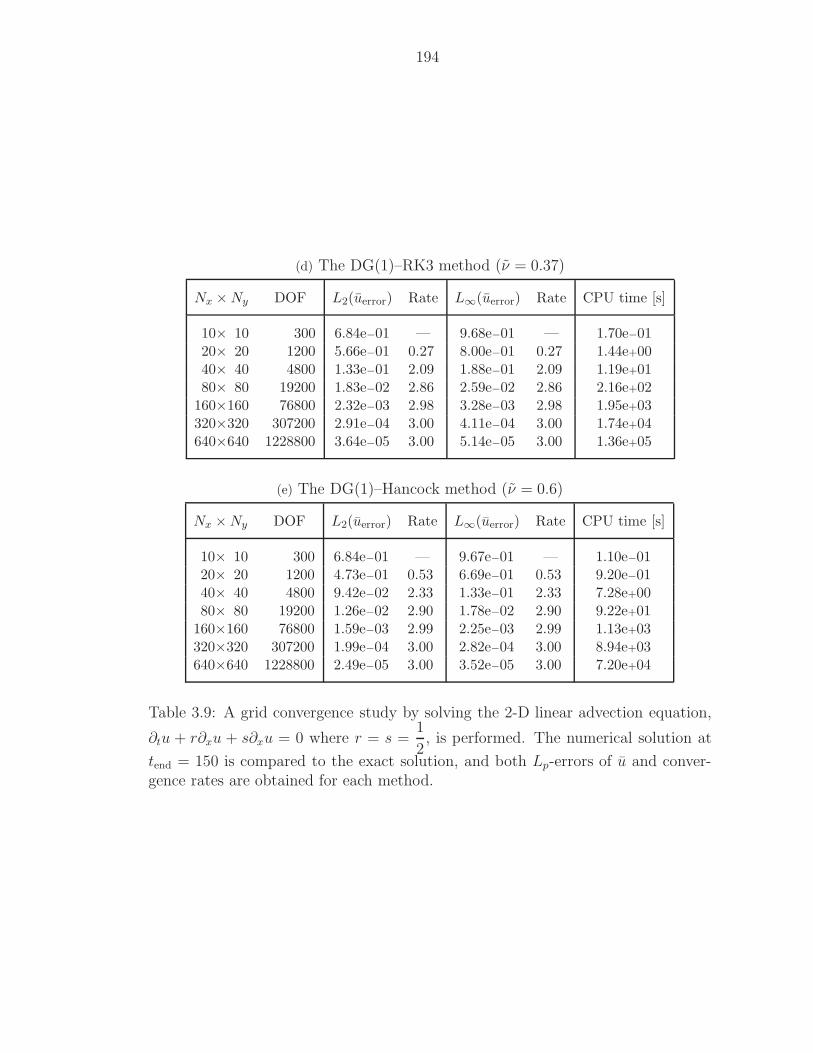
194
(d) The DG(1)–RK3 method (ν = 0.37)
Nx ×Ny DOF L2(uerror) Rate L∞(uerror) Rate CPU time [s]
10× 10 300 6.84e−01 — 9.68e−01 — 1.70e−0120× 20 1200 5.66e−01 0.27 8.00e−01 0.27 1.44e+0040× 40 4800 1.33e−01 2.09 1.88e−01 2.09 1.19e+0180× 80 19200 1.83e−02 2.86 2.59e−02 2.86 2.16e+02
160×160 76800 2.32e−03 2.98 3.28e−03 2.98 1.95e+03320×320 307200 2.91e−04 3.00 4.11e−04 3.00 1.74e+04640×640 1228800 3.64e−05 3.00 5.14e−05 3.00 1.36e+05
(e) The DG(1)–Hancock method (ν = 0.6)
Nx ×Ny DOF L2(uerror) Rate L∞(uerror) Rate CPU time [s]
10× 10 300 6.84e−01 — 9.67e−01 — 1.10e−0120× 20 1200 4.73e−01 0.53 6.69e−01 0.53 9.20e−0140× 40 4800 9.42e−02 2.33 1.33e−01 2.33 7.28e+0080× 80 19200 1.26e−02 2.90 1.78e−02 2.90 9.22e+01
160×160 76800 1.59e−03 2.99 2.25e−03 2.99 1.13e+03320×320 307200 1.99e−04 3.00 2.82e−04 3.00 8.94e+03640×640 1228800 2.49e−05 3.00 3.52e−05 3.00 7.20e+04
Table 3.9: A grid convergence study by solving the 2-D linear advection equation,
∂tu + r∂xu + s∂xu = 0 where r = s =1
2, is performed. The numerical solution at
tend = 150 is compared to the exact solution, and both Lp-errors of u and conver-gence rates are obtained for each method.
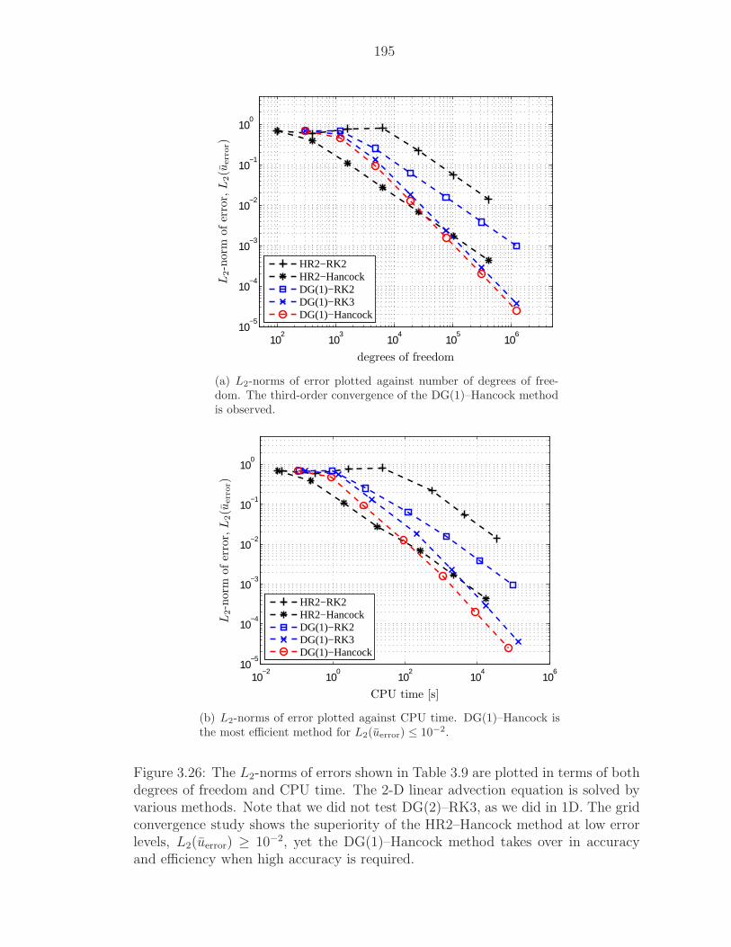
195
102
103
104
105
106
10−5
10−4
10−3
10−2
10−1
100
HR2−RK2HR2−HancockDG(1)−RK2DG(1)−RK3DG(1)−Hancock
degrees of freedom
L2-n
orm
ofer
ror,L
2(u
err
or)
(a) L2-norms of error plotted against number of degrees of free-dom. The third-order convergence of the DG(1)–Hancock methodis observed.
10−2
100
102
104
106
10−5
10−4
10−3
10−2
10−1
100
HR2−RK2HR2−HancockDG(1)−RK2DG(1)−RK3DG(1)−Hancock
CPU time [s]
L2-n
orm
ofer
ror,L
2(u
err
or)
(b) L2-norms of error plotted against CPU time. DG(1)–Hancock isthe most efficient method for L2(uerror) ≤ 10−2.
Figure 3.26: The L2-norms of errors shown in Table 3.9 are plotted in terms of bothdegrees of freedom and CPU time. The 2-D linear advection equation is solved byvarious methods. Note that we did not test DG(2)–RK3, as we did in 1D. The gridconvergence study shows the superiority of the HR2–Hancock method at low errorlevels, L2(uerror) ≥ 10−2, yet the DG(1)–Hancock method takes over in accuracyand efficiency when high accuracy is required.
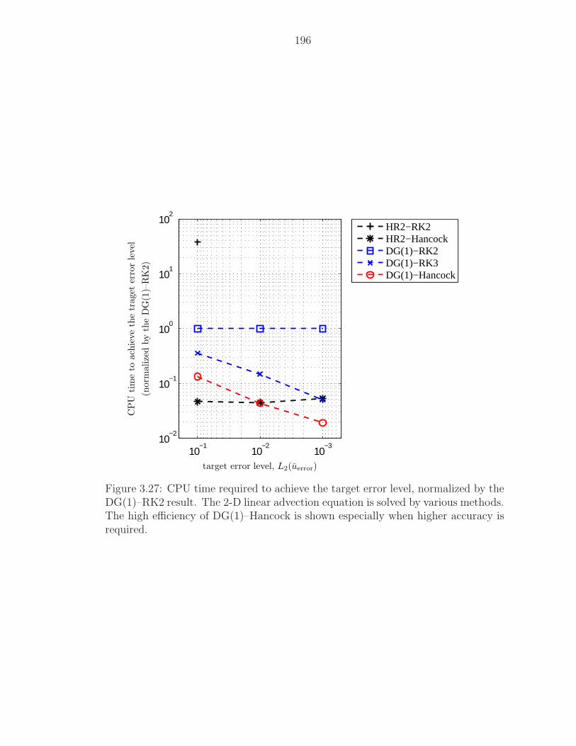
196
10−3
10−2
10−1
10−2
10−1
100
101
102
HR2−RK2HR2−HancockDG(1)−RK2DG(1)−RK3DG(1)−Hancock
target error level, L2(uerror)
CP
Utim
eto
ach
ieve
the
traget
erro
rle
vel
(norm
alize
dby
the
DG
(1)–
RK
2)
Figure 3.27: CPU time required to achieve the target error level, normalized by theDG(1)–RK2 result. The 2-D linear advection equation is solved by various methods.The high efficiency of DG(1)–Hancock is shown especially when higher accuracy isrequired.
197
3.7 Grid Convergence Study for Nonlinear Hyperbolic Equa-tions
3.7.1 The Inviscid Burgers’ Equation
To extend the analysis to nonlinear equations, the inviscid Burgers’ equation:
∂u(x, t)
∂t+
∂
∂x
(1
2u2
)= 0; x ∈ R, t > 0, (3.230)
which represents the simplest model of the motion of a fluid is considered. The
nonlinearity in the flux term leads to the non-constant wave propagation speed u
unlike the constant speed in the linear advection equation. Thus the shape of the
initial-value distribution is no longer preserved, and it creates either a discontinu-
ity (shock) or a smooth profile (expansion). Also, a sufficiently smooth initial condi-
tion could still generate a discontinuity within a finite time due to the nonlinearity.
Here, our motivation is to assess the order of convergence of a numerical method,
therefore, an initial condition that only creates an expansion wave is chosen. The
initial condition is given by
u(x, 0) =
−1 x ≤ −5,
tanh
(10x
25 − x2
)−5 < x < 5,
1 x ≥ 5.
(3.231)
The exact solution in the general form can be constructed by the method of char-
acteristics, and is given by an implicit relation:
u(x, t) = u(x − ut, 0). (3.232)
Note that, in general, the above exact solution is only valid before a shock is formed,
but with the initial values (3.231) this is not a concern. The exact solution at time
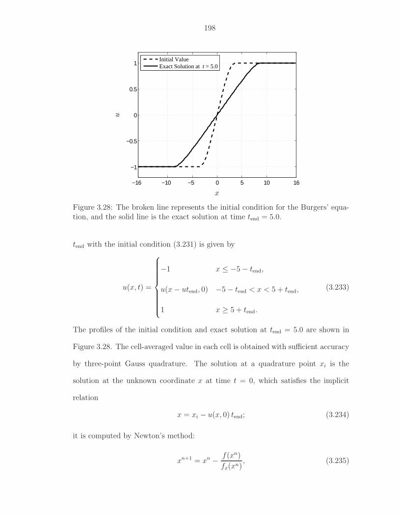
198
−16 −10 −5 0 5 10 16
−1
−0.5
0
0.5
1
Initial ValueExact Solution at t = 5.0
x
u
Figure 3.28: The broken line represents the initial condition for the Burgers’ equa-tion, and the solid line is the exact solution at time tend = 5.0.
tend with the initial condition (3.231) is given by
u(x, t) =
−1 x ≤ −5 − tend,
u(x − utend, 0) −5 − tend < x < 5 + tend,
1 x ≥ 5 + tend.
(3.233)
The profiles of the initial condition and exact solution at tend = 5.0 are shown in
Figure 3.28. The cell-averaged value in each cell is obtained with sufficient accuracy
by three-point Gauss quadrature. The solution at a quadrature point xi is the
solution at the unknown coordinate x at time t = 0, which satisfies the implicit
relation
x = xi − u(x, 0) tend; (3.234)
it is computed by Newton’s method:
xn+1 = xn − f(xn)
fx(xn), (3.235)
199
where
f(x) = x + tanh
(10x
25 − x2
)tend − xi, (3.236a)
fx(x) =10(x2 + 25)
(x2 − 25)2sech2
(10x
25 − x2
). (3.236b)
The Courant number for each method is identical to the value used in the case
of one-dimensional linear advection, equation (3.227) on page 185, that is: 90%
of its stability limit. The L1-,L∞-norms, and corresponding CPU time are listed
in Tables 3.10 and 3.11. Table 3.10 shows that DG(1)–RK3 and DG(2)–RK3 are
third-order accurate, and HR2–RK2, HR2–Hancock, and DG(1)–RK2 are second-
order accurate in both L1- and L∞-norms. Thus, the order of accuracy obtained by
the linear analysis is preserved for a scalar nonlinear problem.
Table 3.11 shows a grid-convergence study of the DG(1)–Hancock method with
various volume-integral treatments. Two quadratures in time, Gauss–Lobatto and
Gauss–Radau, are compared for the nonlinear flux; recall that these two quadratures
give identical results for a linear flux. See Figure 2.3 on page 40 for their quadrature
points in space-time domain.
The sequence of quadratures applied in space and time is examined for its influ-
ence on the order of accuracy. For the spatial integration in the volume integral of
the flux, the Gauss–Lobatto quadrature is always used. Tables 3.11 (a) and (c) show
the result when either the Gauss–Lobatto/Radau temporal quadratures are made
first, then a spatial quadrature is made later. Conversely, Tables 3.11 (b) and (d)
show the result when a spatial quadrature is made first at each time level, then
a temporal quadrature is applied. For instance, in the case of Table 3.11 (d), the
200
volume integral of flux is obtained by the Gauss–Radau quadrature in time
∫∫
Ij×T n
f(u) dxdt ≈ ∆t
4
(3fn+1/3 + fn+1
), (3.237)
where spatially averaged fluxes at time levels n +1
3and n + 1 are computed by
fn+1/3 =∆x
6
[f(u
n+1/3j+1/2 ) + 4f(u
n+1/3j ) + f(u
n+1/3j+1/2 )
], (3.238a)
fn+1 =∆x
6
[f(un+1
j+1/2) + 4f(un+1j ) + f(un+1
j+1/2)]. (3.238b)
Table 3.11 shows that the order of accuracy is sensitive to the sequence of spatial
and temporal quadratures, while both Gauss–Lobatto and Gauss–Radau quadra-
tures in time, when combined in the same sequence, provide similar error levels.
Computing a spatial quadrature first is necessary to achieve higher-order accuracy;
the convergence rates based on the L1-norms of error shows third-order convergence
in this case, yet L∞-norms converge only at the second-order.
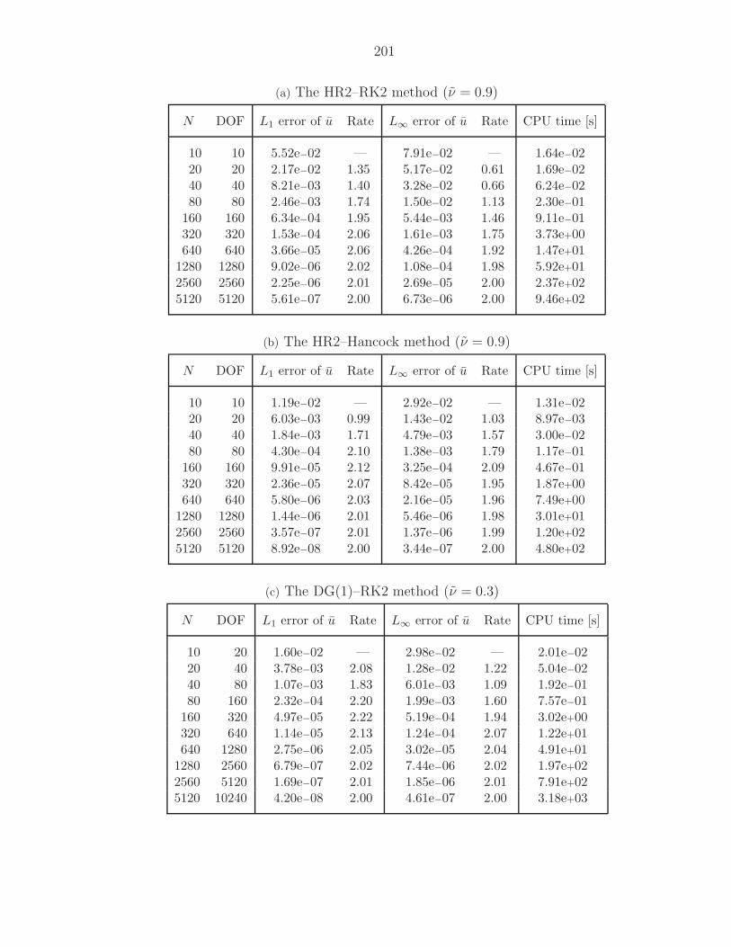
201
(a) The HR2–RK2 method (ν = 0.9)
N DOF L1 error of u Rate L∞ error of u Rate CPU time [s]
10 10 5.52e−02 — 7.91e−02 — 1.64e−0220 20 2.17e−02 1.35 5.17e−02 0.61 1.69e−0240 40 8.21e−03 1.40 3.28e−02 0.66 6.24e−0280 80 2.46e−03 1.74 1.50e−02 1.13 2.30e−01
160 160 6.34e−04 1.95 5.44e−03 1.46 9.11e−01320 320 1.53e−04 2.06 1.61e−03 1.75 3.73e+00640 640 3.66e−05 2.06 4.26e−04 1.92 1.47e+01
1280 1280 9.02e−06 2.02 1.08e−04 1.98 5.92e+012560 2560 2.25e−06 2.01 2.69e−05 2.00 2.37e+025120 5120 5.61e−07 2.00 6.73e−06 2.00 9.46e+02
(b) The HR2–Hancock method (ν = 0.9)
N DOF L1 error of u Rate L∞ error of u Rate CPU time [s]
10 10 1.19e−02 — 2.92e−02 — 1.31e−0220 20 6.03e−03 0.99 1.43e−02 1.03 8.97e−0340 40 1.84e−03 1.71 4.79e−03 1.57 3.00e−0280 80 4.30e−04 2.10 1.38e−03 1.79 1.17e−01
160 160 9.91e−05 2.12 3.25e−04 2.09 4.67e−01320 320 2.36e−05 2.07 8.42e−05 1.95 1.87e+00640 640 5.80e−06 2.03 2.16e−05 1.96 7.49e+00
1280 1280 1.44e−06 2.01 5.46e−06 1.98 3.01e+012560 2560 3.57e−07 2.01 1.37e−06 1.99 1.20e+025120 5120 8.92e−08 2.00 3.44e−07 2.00 4.80e+02
(c) The DG(1)–RK2 method (ν = 0.3)
N DOF L1 error of u Rate L∞ error of u Rate CPU time [s]
10 20 1.60e−02 — 2.98e−02 — 2.01e−0220 40 3.78e−03 2.08 1.28e−02 1.22 5.04e−0240 80 1.07e−03 1.83 6.01e−03 1.09 1.92e−0180 160 2.32e−04 2.20 1.99e−03 1.60 7.57e−01
160 320 4.97e−05 2.22 5.19e−04 1.94 3.02e+00320 640 1.14e−05 2.13 1.24e−04 2.07 1.22e+01640 1280 2.75e−06 2.05 3.02e−05 2.04 4.91e+01
1280 2560 6.79e−07 2.02 7.44e−06 2.02 1.97e+022560 5120 1.69e−07 2.01 1.85e−06 2.01 7.91e+025120 10240 4.20e−08 2.00 4.61e−07 2.00 3.18e+03
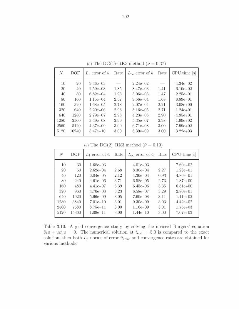
202
(d) The DG(1)–RK3 method (ν = 0.37)
N DOF L1 error of u Rate L∞ error of u Rate CPU time [s]
10 20 9.36e−03 — 2.24e−02 — 4.34e−0220 40 2.59e−03 1.85 8.47e−03 1.41 6.10e−0240 80 6.82e−04 1.93 3.06e−03 1.47 2.25e−0180 160 1.15e−04 2.57 9.56e−04 1.68 8.89e−01
160 320 1.68e−05 2.78 2.07e−04 2.21 3.08e+00320 640 2.20e−06 2.93 3.16e−05 2.71 1.24e+01640 1280 2.79e−07 2.98 4.23e−06 2.90 4.95e+01
1280 2560 3.49e−08 2.99 5.35e−07 2.98 1.99e+022560 5120 4.37e−09 3.00 6.71e−08 3.00 7.99e+025120 10240 5.47e−10 3.00 8.39e−09 3.00 3.22e+03
(e) The DG(2)–RK3 method (ν = 0.19)
N DOF L1 error of u Rate L∞ error of u Rate CPU time [s]
10 30 1.68e−03 — 4.01e−03 — 7.60e−0220 60 2.62e−04 2.68 8.30e−04 2.27 1.28e−0140 120 6.04e−05 2.12 4.36e−04 0.93 4.86e−0180 240 4.61e−06 3.71 6.58e−05 2.73 1.87e+00
160 480 4.41e−07 3.39 6.45e−06 3.35 6.81e+00320 960 4.70e−08 3.23 6.58e−07 3.29 2.80e+01640 1920 5.66e−09 3.05 7.60e−08 3.11 1.11e+02
1280 3840 7.01e−10 3.01 9.30e−09 3.03 4.42e+022560 7680 8.75e−11 3.00 1.16e−09 3.01 1.76e+035120 15360 1.09e−11 3.00 1.44e−10 3.00 7.07e+03
Table 3.10: A grid convergence study by solving the inviscid Burgers’ equation∂tu + u∂xu = 0. The numerical solution at tend = 5.0 is compared to the exactsolution, then both Lp-norms of error uerror and convergence rates are obtained forvarious methods.
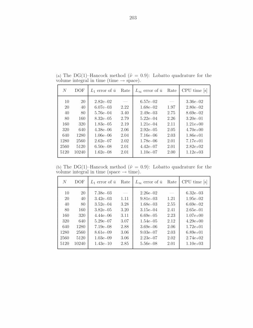
203
(a) The DG(1)–Hancock method (ν = 0.9): Lobatto quadrature for thevolume integral in time (time → space).
N DOF L1 error of u Rate L∞ error of u Rate CPU time [s]
10 20 2.82e−02 — 6.57e−02 — 3.36e−0220 40 6.07e−03 2.22 1.68e−02 1.97 2.80e−0240 80 5.76e−04 3.40 2.49e−03 2.75 8.69e−0280 160 8.32e−05 2.79 5.22e−04 2.26 3.20e−01
160 320 1.83e−05 2.19 1.21e−04 2.11 1.21e+00320 640 4.38e−06 2.06 2.92e−05 2.05 4.70e+00640 1280 1.06e−06 2.04 7.16e−06 2.03 1.86e+01
1280 2560 2.62e−07 2.02 1.78e−06 2.01 7.17e+012560 5120 6.50e−08 2.01 4.42e−07 2.01 2.82e+025120 10240 1.62e−08 2.01 1.10e−07 2.00 1.12e+03
(b) The DG(1)–Hancock method (ν = 0.9): Lobatto quadrature for thevolume integral in time (space → time).
N DOF L1 error of u Rate L∞ error of u Rate CPU time [s]
10 20 7.38e−03 — 2.26e−02 — 6.32e−0320 40 3.42e−03 1.11 9.81e−03 1.21 1.95e−0240 80 3.52e−04 3.28 1.68e−03 2.55 6.69e−0280 160 3.82e−05 3.20 3.15e−04 2.41 2.65e−01
160 320 4.44e−06 3.11 6.69e−05 2.23 1.07e+00320 640 5.29e−07 3.07 1.54e−05 2.12 4.29e+00640 1280 7.19e−08 2.88 3.69e−06 2.06 1.72e+01
1280 2560 8.61e−09 3.06 9.03e−07 2.03 6.89e+012560 5120 1.03e−09 3.06 2.23e−07 2.02 2.74e+025120 10240 1.43e−10 2.85 5.56e−08 2.01 1.10e+03
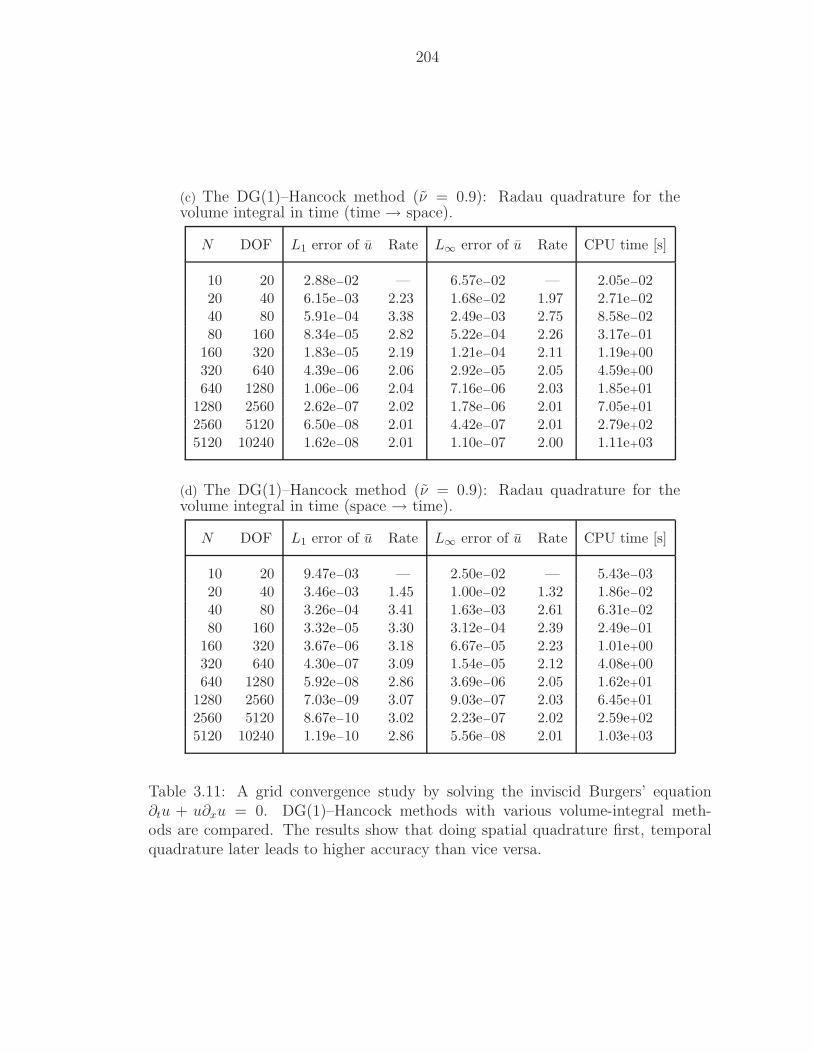
204
(c) The DG(1)–Hancock method (ν = 0.9): Radau quadrature for thevolume integral in time (time → space).
N DOF L1 error of u Rate L∞ error of u Rate CPU time [s]
10 20 2.88e−02 — 6.57e−02 — 2.05e−0220 40 6.15e−03 2.23 1.68e−02 1.97 2.71e−0240 80 5.91e−04 3.38 2.49e−03 2.75 8.58e−0280 160 8.34e−05 2.82 5.22e−04 2.26 3.17e−01
160 320 1.83e−05 2.19 1.21e−04 2.11 1.19e+00320 640 4.39e−06 2.06 2.92e−05 2.05 4.59e+00640 1280 1.06e−06 2.04 7.16e−06 2.03 1.85e+01
1280 2560 2.62e−07 2.02 1.78e−06 2.01 7.05e+012560 5120 6.50e−08 2.01 4.42e−07 2.01 2.79e+025120 10240 1.62e−08 2.01 1.10e−07 2.00 1.11e+03
(d) The DG(1)–Hancock method (ν = 0.9): Radau quadrature for thevolume integral in time (space → time).
N DOF L1 error of u Rate L∞ error of u Rate CPU time [s]
10 20 9.47e−03 — 2.50e−02 — 5.43e−0320 40 3.46e−03 1.45 1.00e−02 1.32 1.86e−0240 80 3.26e−04 3.41 1.63e−03 2.61 6.31e−0280 160 3.32e−05 3.30 3.12e−04 2.39 2.49e−01
160 320 3.67e−06 3.18 6.67e−05 2.23 1.01e+00320 640 4.30e−07 3.09 1.54e−05 2.12 4.08e+00640 1280 5.92e−08 2.86 3.69e−06 2.05 1.62e+01
1280 2560 7.03e−09 3.07 9.03e−07 2.03 6.45e+012560 5120 8.67e−10 3.02 2.23e−07 2.02 2.59e+025120 10240 1.19e−10 2.86 5.56e−08 2.01 1.03e+03
Table 3.11: A grid convergence study by solving the inviscid Burgers’ equation∂tu + u∂xu = 0. DG(1)–Hancock methods with various volume-integral meth-ods are compared. The results show that doing spatial quadrature first, temporalquadrature later leads to higher accuracy than vice versa.
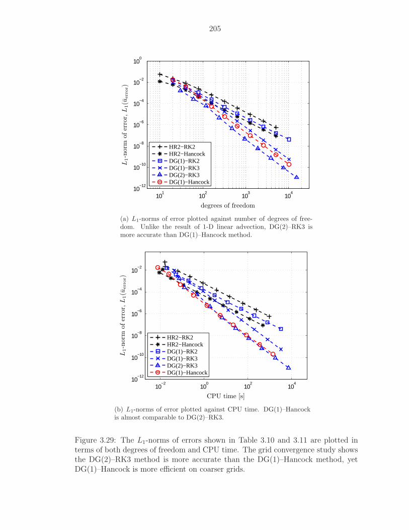
205
101
102
103
104
10−12
10−10
10−8
10−6
10−4
10−2
100
HR2−RK2HR2−HancockDG(1)−RK2DG(1)−RK3DG(2)−RK3DG(1)−Hancock
degrees of freedom
L1-n
orm
ofer
ror,L
1(u
err
or)
(a) L1-norms of error plotted against number of degrees of free-dom. Unlike the result of 1-D linear advection, DG(2)–RK3 ismore accurate than DG(1)–Hancock method.
10−2
100
102
104
10−12
10−10
10−8
10−6
10−4
10−2
HR2−RK2HR2−HancockDG(1)−RK2DG(1)−RK3DG(2)−RK3DG(1)−Hancock
CPU time [s]
L1-n
orm
ofer
ror,L
1(u
err
or)
(b) L1-norms of error plotted against CPU time. DG(1)–Hancockis almost comparable to DG(2)–RK3.
Figure 3.29: The L1-norms of errors shown in Table 3.10 and 3.11 are plotted interms of both degrees of freedom and CPU time. The grid convergence study showsthe DG(2)–RK3 method is more accurate than the DG(1)–Hancock method, yetDG(1)–Hancock is more efficient on coarser grids.
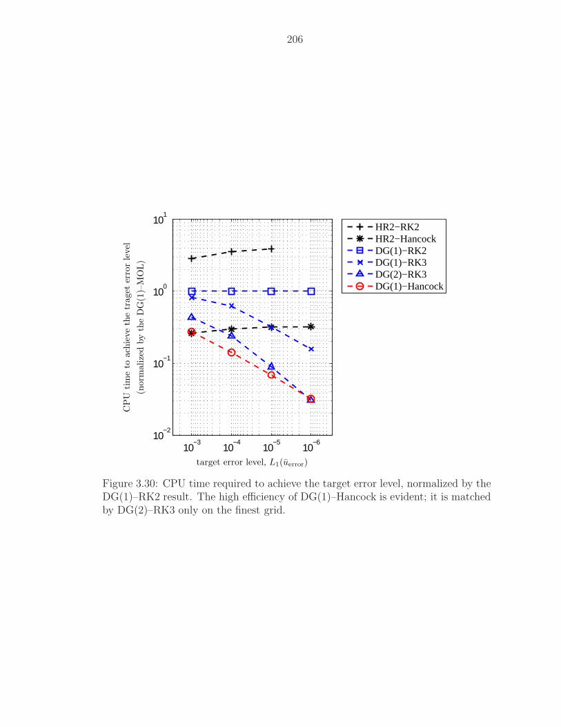
206
10−6
10−5
10−4
10−3
10−2
10−1
100
101
HR2−RK2HR2−HancockDG(1)−RK2DG(1)−RK3DG(2)−RK3DG(1)−Hancock
target error level, L1(uerror)
CP
Utim
eto
ach
ieve
the
traget
erro
rle
vel
(norm
alize
dby
the
DG
(1)–
MO
L)
Figure 3.30: CPU time required to achieve the target error level, normalized by theDG(1)–RK2 result. The high efficiency of DG(1)–Hancock is evident; it is matchedby DG(2)–RK3 only on the finest grid.
CHAPTER IV
ANALYSIS FOR 1-D AND 2-D LINEAR
HYPERBOLIC-RELAXATION EQUATIONS
4.1 Introduction
In this chapter, numerical methods including the DG(1)–Hancock method for
hyperbolic-relaxation equations are investigated analytically and numerically. As
a preliminary analysis for hyperbolic-relaxation equations, various methods for hy-
perbolic conservation laws were analyzed in the previous chapter; Fourier analyses
and numerical tests show the superior accuracy and efficiency of the DG(1)–Hancock
method over the semi-discrete, method-of-lines approach for both linear and nonlin-
ear equations. We shall now carry out a Fourier analysis of four methods applied to
one- and two-dimensional systems of linear hyperbolic-relaxation equations. The lo-
cal truncation error of the DG(1)–Hancock is compared to HR2–MOL, DG(1)–MOL,
and HR2–Hancock; numerical tests confirm the linear analysis. Later, the discretiza-
tion methods are applied to a system of nonlinear hyperbolic-relaxation equations
to examine the validity of the linear analysis.
207
208
4.2 Model Equations: Generalized Hyperbolic Heat Equa-tions
4.2.1 Dimensional Form
The model equation we consider is the generalized hyperbolic heat equations
(GHHE) [JL96, Hit00, LM02],
∂tu + ∂xv = 0, (4.1a)
∂tv + a2F ∂xu = −1
τ(v − aEu); x ∈ R, t > 0, (4.1b)
where u(x, t) ∈ R is the conserved variable and v(x, t) ∈ R is the flux of u. In vector
form, u = [u, v]T , f = [v, a2F u]T , and s = [0, aEu − v]T in
∂tu + ∂xf(u) =1
τs(u). (4.2)
There are three constant parameters: τ > 0 is a relaxation time, aF > 0 is a frozen
wave speed, and aE > 0 is an equilibrium wave speed. For stability, |aE| ≤ aF . The
constant Jacobian matrix and its eigenvalues are as follows:
A :=∂f
∂u=
0 1
a2F 0
−→ λ1,2 := Eig(A) = ±aF . (4.3)
Here, we insist that these three parameters have physical meaning; once the problem
is described, these parameters are fixed. The above equations are constructed such
that the frozen waves propagate at speed ±aF in the beginning; these eventually
decay. Simultaneously, equilibrium waves at speed ±aE enter the model; one of
the equilibrium waves with speed −aE is quickly damped out, and the other wave
with speed aE dominates the solution. Figure 4.1 describes these waves schemati-
cally. The right hand side of (4.1) represents the relaxation process, which always
drives the non-equilibrium flux variable v to its equilibrium flux aEu. A detailed
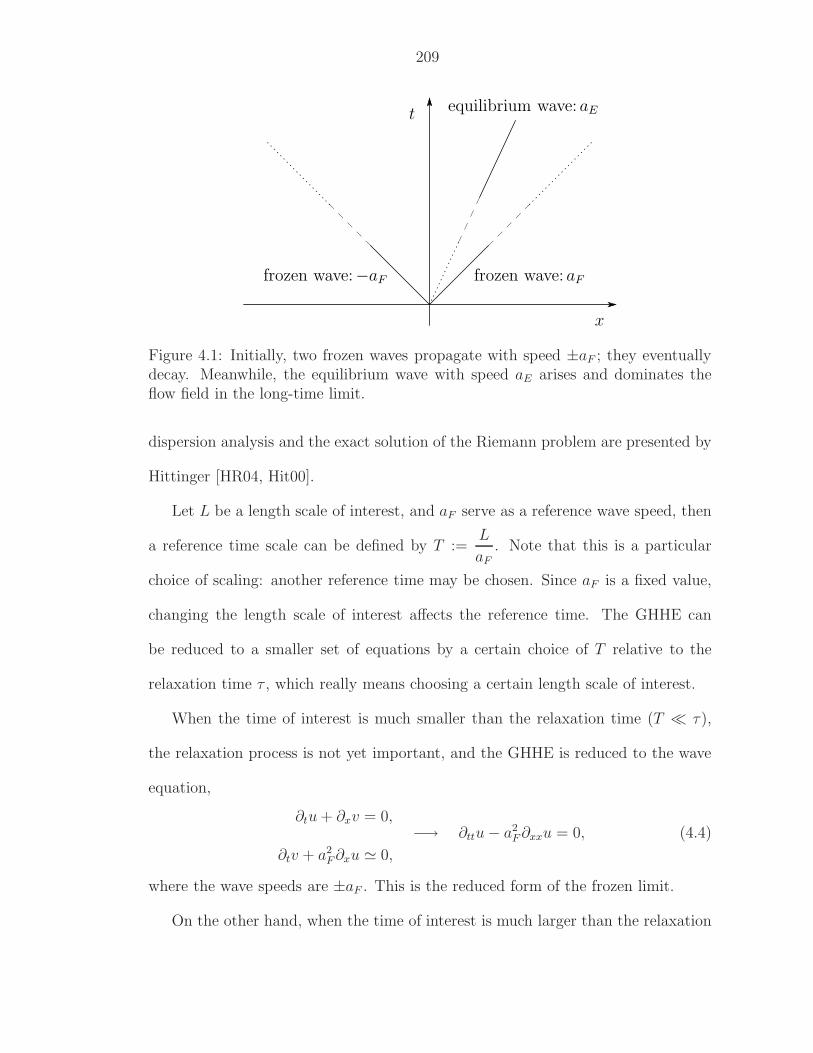
209
x
t
frozen wave: aFfrozen wave:−aF
equilibrium wave: aE
Figure 4.1: Initially, two frozen waves propagate with speed ±aF ; they eventuallydecay. Meanwhile, the equilibrium wave with speed aE arises and dominates theflow field in the long-time limit.
dispersion analysis and the exact solution of the Riemann problem are presented by
Hittinger [HR04, Hit00].
Let L be a length scale of interest, and aF serve as a reference wave speed, then
a reference time scale can be defined by T :=L
aF
. Note that this is a particular
choice of scaling: another reference time may be chosen. Since aF is a fixed value,
changing the length scale of interest affects the reference time. The GHHE can
be reduced to a smaller set of equations by a certain choice of T relative to the
relaxation time τ , which really means choosing a certain length scale of interest.
When the time of interest is much smaller than the relaxation time (T ≪ τ),
the relaxation process is not yet important, and the GHHE is reduced to the wave
equation,
∂tu + ∂xv = 0,
∂tv + a2F∂xu ≃ 0,
−→ ∂ttu − a2F ∂xxu = 0, (4.4)
where the wave speeds are ±aF . This is the reduced form of the frozen limit.
On the other hand, when the time of interest is much larger than the relaxation
210
time (T ≫ τ), the relaxation process is no longer negligible. Asymptotic expansion
of u and v for small τ gives an advection-diffusion equation (the derivation for the
particular scaling is given in Appendix C on page 354):
∂tu + aE∂xu = τ(a2F − a2
E)∂xxu + O(τ 2). (4.5)
This is the reduced form in the near-equilibrium limit. Note that the leading dif-
fusion coefficient τ(a2F − a2
E) always has a positive sign as long as aE ≤ aF ; this
property is called the sub-characteristic condition for stability [Liu87]. There are
two different physical processes included in this equation; the relative strength of
the two parameters, advection speed aE and diffusion coefficient ǫ(a2F −a2
E), decides
which is the dominant physics. This will be discussed in more detail in a later
section.
We further consider the time scale of interest T to be infinite; this is equivalent
to letting τ → 0, so the relaxation process occurs instantaneously, and the above
equation becomes a pure advection equation:
∂tu + aE∂xu = 0, (4.6)
where the wave speed is aE. This is the reduced form of the GHHE in the equilibrium
limit.
To summarize, let t be the dimensionless time normalized by the relaxation time
τ such that
t :=T
τ=
L
aF τ. (4.7)
The reduced equations of the GHHE corresponding to t are shown in Table 4.1.
These forms can be seen as consecutive transformations of the GHHE in the time
frame.
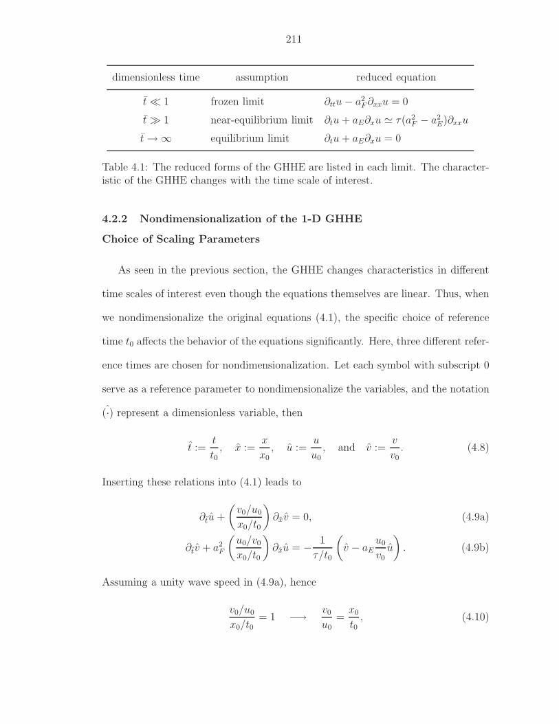
211
dimensionless time assumption reduced equation
t ≪ 1 frozen limit ∂ttu − a2F ∂xxu = 0
t ≫ 1 near-equilibrium limit ∂tu + aE∂xu ≃ τ(a2F − a2
E)∂xxu
t → ∞ equilibrium limit ∂tu + aE∂xu = 0
Table 4.1: The reduced forms of the GHHE are listed in each limit. The character-istic of the GHHE changes with the time scale of interest.
4.2.2 Nondimensionalization of the 1-D GHHE
Choice of Scaling Parameters
As seen in the previous section, the GHHE changes characteristics in different
time scales of interest even though the equations themselves are linear. Thus, when
we nondimensionalize the original equations (4.1), the specific choice of reference
time t0 affects the behavior of the equations significantly. Here, three different refer-
ence times are chosen for nondimensionalization. Let each symbol with subscript 0
serve as a reference parameter to nondimensionalize the variables, and the notation
(·) represent a dimensionless variable, then
t :=t
t0, x :=
x
x0, u :=
u
u0, and v :=
v
v0. (4.8)
Inserting these relations into (4.1) leads to
∂tu +
(v0/u0
x0/t0
)∂xv = 0, (4.9a)
∂tv + a2F
(u0/v0
x0/t0
)∂xu = − 1
τ/t0
(v − aE
u0
v0u
). (4.9b)
Assuming a unity wave speed in (4.9a), hence
v0/u0
x0/t0= 1 −→ v0
u0=
x0
t0, (4.10)
212
does not change the problem, and the above equations become
∂tu + ∂xv = 0, (4.11a)
∂tv +
(aF
x0/t0
)2
∂xu = − 1
τ/t0
(v − aE
x0/t0u
). (4.11b)
Now, the proper reference time t0 and reference speedx0
t0have to be chosen for the
nondimensionalization. Available constant parameters are aF [LT−1], aE [LT−1],
and τ [T]. Also, let L [L] be a length scale of interest, which may vary within a
problem. As to a reference time, the obvious choice is t0 = τ ; in this scaling, time
is measured at a scale of the same order of the relaxation process. A next possible
scaling is t0 =L
aF
where time is scaled by the traveling time of frozen waves. The
equilibrium speed can be used as scaling when aE 6= 0, thus t0 =L
aE
. Note that
L
aF
≤ L
aE
. Another nonintuitive choice is t0 =L2
τa2F
.
As a reference speedx0
t0, both frozen speed aF and equilibrium speed aE are the
obvious choices; the characteristic speed of relaxationL
τmight be a possible choice
as well. The specific forms of each scaling are discussed in the next section under
the assumption u0 = O(1).
Scaling 1: Relaxation Time Scale (t0 = τ)
Choosing the relaxation time as the reference time (t0 = τ) eliminates the τ
dependence in the equations when frozen wave speed is selected as reference speed
x0/t0 = aF , the dimensionless variables (4.8) become
t =t
τ, x =
x
aF τ, u =
u
u0
, and v =v
aF u0
, (4.12)
and we set t = u = O(1). In this scaling, the dimensionless GHHE (4.11) becomes
∂tu + ∂xv = 0, (4.13a)
∂tv + ∂xu = −(v − ru), (4.13b)
213
where
r :=aE
aF
, |r| ≤ 1, (4.14)
is the dimensionless equilibrium speed. Note that in this scaling, there is no reduced
asymptotic form since the time scale of interest is set to be that of relaxation process.
Scaling 2: Frozen-Wave Time Scale (t0 = L/aF )
In this scaling, the reference time is scaled by t0 =L
aF
, and the frozen wave
speed aF is chosen as the reference speed. Then, the dimensionless variables (4.8)
become
t =t
L/aF, x =
x
L, u =
u
u0, and v =
v
aF u0, (4.15)
and we set t = u = O(1). Under these scaling, the dimensionless GHHE become
∂tu + ∂xv = 0, (4.16a)
∂tv + ∂xu = −1
ǫ(v − ru), (4.16b)
where
ǫ :=τaF
L> 0, (4.17)
is the dimensionless relaxation time, and r is defined by (4.14). Recall that both
τ and aF are fixed, yet L could be changed. Thus, ǫ is a function of the length
scale of interest L. We are particularly interested in the nondimensional form of
the GHHE in this frozen-wave time scale since the above equations reduce to the
advection-dominated advection-diffusion equation,
∂tu + r∂xu = ǫ (1 − r2)∂xxu + O(ǫ2), (4.18)
in the near-equilibrium limit (ǫ ≪ O(1)); the derivation is shown in Appendix C on
page 354. Note that the inverse of the dimensionless relaxation time ǫ can be seen
214
as the dimensionless time t defied by (4.7):
1
ǫ=
L/aF
τ=
T
τ→ t ≡ 1
ǫ. (4.19)
Hence, the smaller the relaxation time ǫ, the longer the time scale for the GHHE,
and eventually the GHHE reduces to the advection equation in the limit where
ǫ → 0.
Scaling 3: Equilibrium-Wave Time Scale (t0 = L/aE)
In this scaling, the reference time is scaled by t0 =L
aE, and the equilibrium
wave speed aE is chosen as reference speed. Thus, the dimensionless variables (4.8)
become
t =t
L/aE, x =
x
L, u =
u
u0, and v =
v
aEu0, (4.20)
and we set t = u = O(1). Under these scaling, the dimensionless GHHE becomes
∂tu + ∂xv = 0, (4.21a)
∂tv +1
r2∂xu = − 1
ǫr(v − u), (4.21b)
where r and ǫ are defined by (4.14) and (4.17), respectively. The reduced equation
in the near-equilibrium limit is
∂tu + ∂xu =ǫ (1 − r2)
r∂xxu + O
(ǫ2), (4.22)
where the dimensionless advection speed is 1, and the viscosity is the inverse of the
Peclet number defined by
Pe :=r
ǫ (1 − r2). (4.23)
Relation of Dimensionless Parameters
Even though we are interested in the frozen-time scale (4.16), and further anal-
ysis focusses on this scaling, the results can be transformed to other scales by using
215
the following relations:
frozen-wave time → relaxation time:
t =t
ǫ, x =
x
ǫ, u = u, and v = v, (4.24a)
frozen-wave time → equilibrium-wave time:
t = rt, x = x, u = u, and v =v
r. (4.24b)
4.2.3 Nondimensional Form
Symmetric Frozen-Wave-Speeds Model
Among the various nondimensionalization, we adopt the second scaling, frozen-
wave time scale, for the following analysis. For simplicity, the notation (·) is hence-
forth omitted, and our target model equations are written as
∂tu + ∂xv = 0, (4.25a)
∂tv + ∂xu = −1
ǫ(v − ru). (4.25b)
Here, u is the conserved variable, v is the flux of u, and ǫ > 0 is a dimensionless
relaxation time. In vector form, u = [u, v]T , f = [v, u]T , and s = [0, ru − v]T in
∂tu + ∂xf(u) =1
ǫs(u). (4.26)
This system has ‘frozen’ wave speeds ±1 when relaxation is weak (ǫ ≫ 1); when
relaxation dominates (ǫ ≪ 1), it reduces to the advection-diffusion equation,
∂tu + r∂xu = ǫ(1 − r2)∂xxu + O(ǫ2), (4.27)
with an ‘equilibrium’ wave speed r. For stability, |r| ≤ 1. Note that we have
written this equation in a form that leads to an advection-dominated advection-
diffusion asymptotic limit. This is consistent with a focus on compressible, viscous
216
flow. Other choices of scalings, such as diffusive scalings [LM02, NP00], can lead
to more strongly parabolic limits. Indeed, for r = O(ǫ), the scaling of Lowrie and
Morel [LM02] is in effect a long-time, small-advective-flux limit.
Asymmetric Frozen-Wave-Speeds Model
The system (4.25) can be generalized to break symmetry in the frozen limit
[HSvL05]:
∂tu + ∂xv = 0, (4.28a)
∂tv + c∂xu + (1 − c)∂xv = −1
ǫ(v − ru). (4.28b)
The frozen wave speeds are thus −c and 1, and the near-equilibrium form is
∂tu + r∂xu = ǫ(1 − r)(c + r)∂xxu + O(ǫ2). (4.29)
Note the modification to the diffusion rate. For stability, −c ≤ r ≤ 1. This model
is used only for limited cases due to the complexity of analysis.
Exact Solution
In the reduced equation of the GHHE (4.27), the exact eigenvalue of the spatial
differentiation operator for the harmonic mode u(x, t) = u0e(ikx+λt) is given by
λGHHEexact = −irk − ǫ(1 − r2)k2 − 2iǫ2r(1 − r2)k3 + O
(ǫ3). (4.30)
Note that the above exact solution is indeed an infinite series. Conversely, the
exact solution of the spatial differential operator of the genuine advection-diffusion
equation runs only up to O(ǫ2), thus
λadv-diffexact = −irk − ǫ(1 − r2)k2. (4.31)
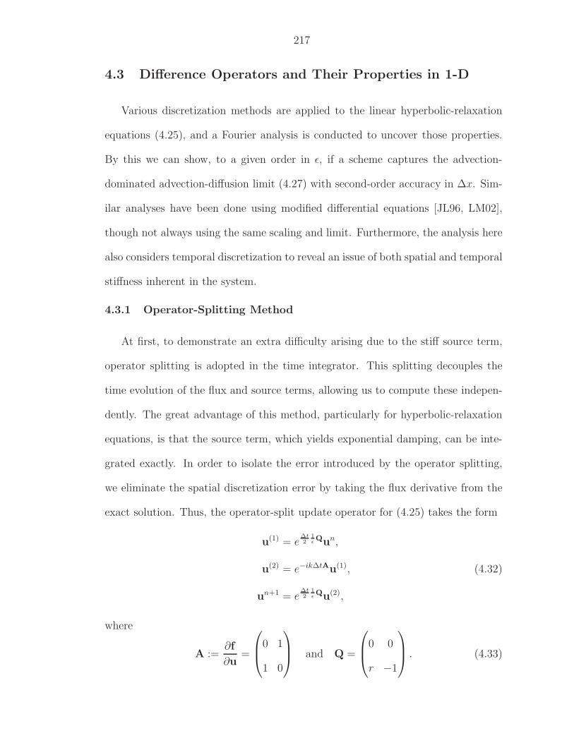
217
4.3 Difference Operators and Their Properties in 1-D
Various discretization methods are applied to the linear hyperbolic-relaxation
equations (4.25), and a Fourier analysis is conducted to uncover those properties.
By this we can show, to a given order in ǫ, if a scheme captures the advection-
dominated advection-diffusion limit (4.27) with second-order accuracy in ∆x. Sim-
ilar analyses have been done using modified differential equations [JL96, LM02],
though not always using the same scaling and limit. Furthermore, the analysis here
also considers temporal discretization to reveal an issue of both spatial and temporal
stiffness inherent in the system.
4.3.1 Operator-Splitting Method
At first, to demonstrate an extra difficulty arising due to the stiff source term,
operator splitting is adopted in the time integrator. This splitting decouples the
time evolution of the flux and source terms, allowing us to compute these indepen-
dently. The great advantage of this method, particularly for hyperbolic-relaxation
equations, is that the source term, which yields exponential damping, can be inte-
grated exactly. In order to isolate the error introduced by the operator splitting,
we eliminate the spatial discretization error by taking the flux derivative from the
exact solution. Thus, the operator-split update operator for (4.25) takes the form
u(1) = e∆t2
1ǫQun,
u(2) = e−ik∆tAu(1), (4.32)
un+1 = e∆t2
1ǫQu(2),
where
A :=∂f
∂u=
0 1
1 0
and Q =
0 0
r −1
. (4.33)
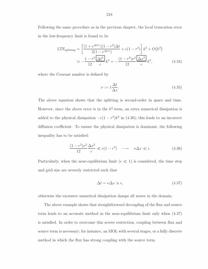
218
Following the same procedure as in the previous chapter, the local truncation error
in the low-frequency limit is found to be
LTEsplitting =
[(1 + e∆t/ǫ)(1 − r2)∆t
2(1 − e∆t/ǫ)+ ǫ(1 − r2)
]k2 + O
(k3)
≃ −1 − r2
12
∆t2
ǫk2 = −(1 − r2)ν2
12
∆x2
ǫk2, (4.34)
where the Courant number is defined by
ν := 1∆t
∆x. (4.35)
The above equation shows that the splitting is second-order in space and time.
However, since the above error is in the k2-term, an extra numerical dissipation is
added to the physical dissipation −ǫ(1 − r2)k2 in (4.30); this leads to an incorrect
diffusion coefficient. To ensure the physical dissipation is dominant, the following
inequality has to be satisfied:
(1 − r2)ν2
12
∆x2
ǫ≪ ǫ(1 − r2) −→ ν∆x ≪ ǫ. (4.36)
Particularly, when the near-equilibrium limit (ǫ ≪ 1) is considered, the time step
and grid size are severely restricted such that
∆t = ν∆x ∝ ǫ, (4.37)
otherwise the excessive numerical dissipation damps all waves in the domain.
The above example shows that straightforward decoupling of the flux and source
term leads to an accurate method in the near-equilibrium limit only when (4.37)
is satisfied. In order to overcome this severe restriction, coupling between flux and
source term is necessary; for instance, an MOL with several stages, or a fully discrete
method in which the flux has strong coupling with the source term.
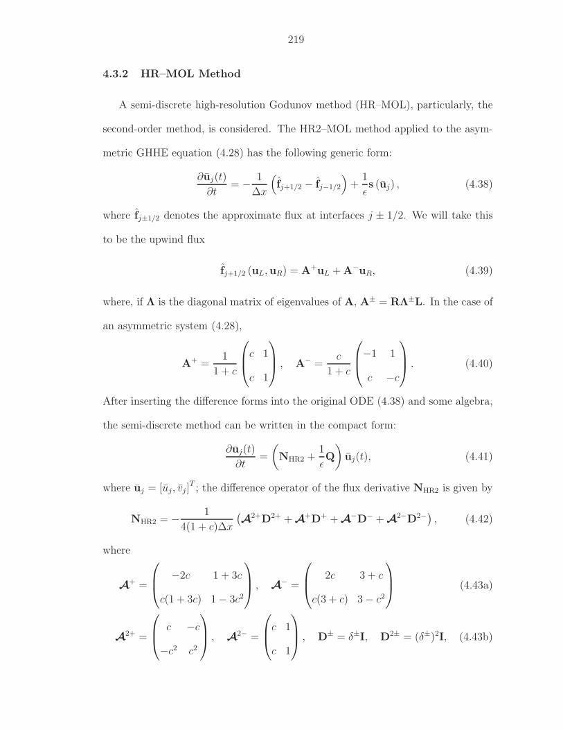
219
4.3.2 HR–MOL Method
A semi-discrete high-resolution Godunov method (HR–MOL), particularly, the
second-order method, is considered. The HR2–MOL method applied to the asym-
metric GHHE equation (4.28) has the following generic form:
∂uj(t)
∂t= − 1
∆x
(fj+1/2 − fj−1/2
)+
1
ǫs (uj) , (4.38)
where fj±1/2 denotes the approximate flux at interfaces j ± 1/2. We will take this
to be the upwind flux
fj+1/2 (uL,uR) = A+uL + A−uR, (4.39)
where, if Λ is the diagonal matrix of eigenvalues of A, A± = RΛ±L. In the case of
an asymmetric system (4.28),
A+ =1
1 + c
c 1
c 1
, A− =
c
1 + c
−1 1
c −c
. (4.40)
After inserting the difference forms into the original ODE (4.38) and some algebra,
the semi-discrete method can be written in the compact form:
∂uj(t)
∂t=
(NHR2 +
1
ǫQ
)uj(t), (4.41)
where uj = [uj, vj ]T ; the difference operator of the flux derivative NHR2 is given by
NHR2 = − 1
4(1 + c)∆x
(A
2+D2+ + A+D+ + A
−D− + A2−D2−
), (4.42)
where
A+ =
−2c 1 + 3c
c(1 + 3c) 1 − 3c2
, A
− =
2c 3 + c
c(3 + c) 3 − c2
(4.43a)
A2+ =
c −c
−c2 c2
, A
2− =
c 1
c 1
, D± = δ±I, D2± = (δ±)2I, (4.43b)
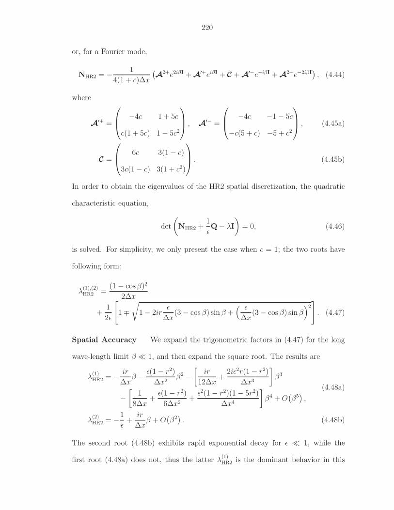
220
or, for a Fourier mode,
NHR2 = − 1
4(1 + c)∆x
(A
2+e2iβI + A′+eiβI + C + A
′−e−iβI + A2−e−2iβI
), (4.44)
where
A′+ =
−4c 1 + 5c
c(1 + 5c) 1 − 5c2
, A
′− =
−4c −1 − 5c
−c(5 + c) −5 + c2
, (4.45a)
C =
6c 3(1 − c)
3c(1 − c) 3(1 + c2)
. (4.45b)
In order to obtain the eigenvalues of the HR2 spatial discretization, the quadratic
characteristic equation,
det
(NHR2 +
1
ǫQ − λI
)= 0, (4.46)
is solved. For simplicity, we only present the case when c = 1; the two roots have
following form:
λ(1),(2)HR2 =
(1 − cos β)2
2∆x
+1
2ǫ
[1 ∓
√1 − 2ir
ǫ
∆x(3 − cos β) sin β +
( ǫ
∆x(3 − cos β) sin β
)2]
. (4.47)
Spatial Accuracy We expand the trigonometric factors in (4.47) for the long
wave-length limit β ≪ 1, and then expand the square root. The results are
λ(1)HR2 = − ir
∆xβ − ǫ(1 − r2)
∆x2β2 −
[ir
12∆x+
2iǫ2r(1 − r2)
∆x3
]β3
−[
1
8∆x+
ǫ(1 − r2)
6∆x2+
ǫ2(1 − r2)(1 − 5r2)
∆x4
]β4 + O
(β5),
(4.48a)
λ(2)HR2 = −1
ǫ+
ir
∆xβ + O
(β2). (4.48b)
The second root (4.48b) exhibits rapid exponential decay for ǫ ≪ 1, while the
first root (4.48a) does not, thus the latter λ(1)HR2 is the dominant behavior in this
221
asymptotic limit. Following the analysis of the linear advection equation in the
previous chapter, the spatial discretization error is obtained by replacing β by the
wave number k :=β
∆x, then
λ(1)HR2 − λGHHE
exact = − ir
12∆x2
︸ ︷︷ ︸dispersion error
k3 −[1
8∆x3 +
ǫ(1 − r2)
6∆x2
]
︸ ︷︷ ︸dissipation error
k4 + O(k5), (4.49a)
λ(2)HR2 − λGHHE
exact = −1
ǫ+ 2irk + O
(k2), (4.49b)
where the exact spatial differential operator λGHHEexact is given in (4.30). In the first
equation, both dispersive (k3-term) and dissipative (k4-term) errors are present;
the dispersive error is second-order in ∆x, and since the correct limit shows no
dispersion, these numerical dispersion errors can not be confused with any physical
dispersion. However, the leading dissipative error term, −1
8∆x3k4, does not scale
with ǫ, and so can compete with the physical dissipation −ǫ (1−r2)k2 in (4.30) if the
relaxation scale is unresolved (∆x ≫ ǫ). For the physical dissipation to dominate,
(dominant numerical dissipation) ≪ (physical dissipation), (4.50)
thus,
1
8∆x3k4 ≪ ǫ(1 − r2)k2. (4.51)
Solving for ∆x leads to the threshold grid size ∆h∗HR2:
∆x ≪ 2
[ǫ(1 − r2)
k2
]1/3
= 2( r
k2 Pe
)1/3
, (4.52)
thus,
∆h∗HR2 := 2
( r
k2 Pe
)1/3
. (4.53)
Hence, the HR2 scheme does not attain the asymptotic limit to second-order in ∆x
with ∆x independent of ǫ.
222
For the HR2 scheme, the result (4.52) is well known. It appears for the r = 0
case in previous studies, [JL96, LM02] although not necessarily in our scaling. The
form (4.49a) for r 6= 0 for the HR2 scheme can be obtained from Eq. (3.17) in Jin
and Levermore [JL96, p. 461] or Eq. (31) in Lowrie and Morel [LM02, p. 420]. In
the scaling of the latter work, the term that leads to (4.52) is actually divergent
since it goes like∆x3
ǫ(due to the time dilation of this scaling), but it still leads
to the constraint (4.52). Jin and Levermore claimed that the grid size restriction
can be removed by averaging the frozen and equilibrium fluxes [Jin95]. However,
we find that the grid restriction still exists in their method. The detailed analysis
is described in Appendix D.
It is interesting to compare (4.52) with a direct discretization of the asymptotic
equation (4.27) on page 215 using the Rusanov flux function and slope reconstruc-
tion. The diffusion term is discretized using a three-point, second-order central-
difference approximation. From a Fourier analysis, the eigenvalue of the scheme
is
λadv-diffHR2 −λadv-diff
exact = − ir
12∆x2 k3 −
[1
8∆x3 − ǫ(1 − r2)
12∆x2
]k4 + O
(k5), (4.54)
for ∆x ≪ 1. We see that this has the same fourth-order numerical dissipation
term as the HR2 discretization of GHHE (4.49a). This discretization will have the
same restriction (4.52) on ∆x to ensure that the physical dissipation is dominant.
When this restriction is satisfied, the above equation shows that the HR2 method
is second-order in space owing to ∆x2 in the k3-term.
Spatial-Temporal Accuracy In our previous analysis, we only consider the
spatial discretization of the HR2 method under the assumption that the flux and
source term are discretized at the same time level [HSvL05]. However, a typically
223
ODE solver for a stiff problem discretizes the flux and source terms at different
time levels due to the implicit treatment of the source term. Furthermore, the
system (4.25) possesses both spatial and temporal stiffness, thus, analyzing a fully
discrete form of any method is necessary. A great number of stiff ODE solvers
have been proposed in the last few decades [Jin95, CJR97, LRR00, NP00, TSL00,
HW96, Lam91]. Among these methods, we adopt the implicit-explicit (IMEX)
Runge–Kutta methods originally developed by Ascher et al. [ARW95, ARS97] for
hyperbolic-parabolic equations, and later extended to hyperbolic-relaxation equa-
tions by Pareschi and Russo [PR05]. The methods treat the flux term explicitly by a
strong-stability-preserving (SSP) method, and the source term by an L-stable diago-
nally implicit Runge–Kutta method (DIRK). The authors developed a family of sec-
ond and third-order methods. Here, as an example, we adopt the IMEX–SSP2(3,3,2)
method; both explicit and implicit methods require three stages, and overall accu-
racy is second-order. The actual update formulas are the following:
u(1) = un +∆t
4ǫs(u(1)),
u(2) = un − ∆t
2∂xf(u
(1)) +∆t
4ǫs(u(2)), (4.55)
u(3) = un − ∆t
2
[∂xf(u
(1)) + ∂xf(u(2))]+
∆t
3ǫ
[s(u(1)) + s(u(2)) + s(u(3))
],
un+1 = un − ∆t
3
[∂xf(u
(1)) + ∂xf(u(2)) + ∂xf(u
(3))]
+∆t
3ǫ
[s(u(1)) + s(u(2)) + s(u(3))
].
The development of the truncation-error analysis is based on the method described
in Chapter III. In order to obtain an explicit form for roots of a characteristic equa-
tion, due to the complexity of any amplification matrix G, we assume a power-series
form for the amplification factor,
gmethod = g0 + g1k + g2k2 + O
(k3), (4.56)
224
for the wave number k ≪ 1. In brief, once an amplification factor g is obtained
from an amplification matrix G, the local truncation error is obtained by
LTEmethod =
∞∑
n=2
cnkn, (4.57)
where the coefficient cn is
cn =1
n!∆tg(k = 0)
∂ng(k)
∂kn
∣∣∣∣k=0
. (4.58)
The intermediate formulas for the derivation of the local truncation error are omitted
here; only the final result is presented. The local truncation error of the HR2–IMEX
method becomes
LTEHR2IMEX =
−
ir
12
(1 + (rν)2
)∆x2
︸ ︷︷ ︸dominant dispersion error
−iǫ r(1 − r2)ν
6∆x
k3
−
1
8
(1 − r
3(rν)3
)∆x3
︸ ︷︷ ︸dominant dissipation error
+ǫ (1 − r2)
6∆x2
k4. (4.59)
Under the assumption of near-equilibrium we have r = O(1) and ǫ ≪ 1; when the
physical dissipation dominates over the dissipation error,
1
8
(1 − r
3(rν)3
)∆x3k4 ≪ ǫ (1 − r2)k2, (4.60)
then the method is second-order in both space and time owing to the dominant
dispersion error in the k3-term. Note that the remaining terms in (4.59) are guar-
anteed to be always smaller than the physical dispersion and dissipation owing to ǫ
in their coefficients. Finally, the threshold grid size for the fully discrete method is
given by
∆h∗HR2IMEX := 2
ǫ(1 − r2)(
1 − r
3(rν)3
)k2
1/3
. (4.61)
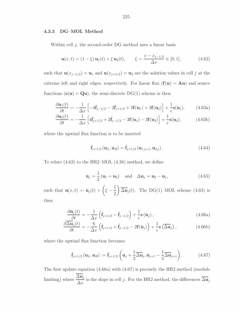
225
4.3.3 DG–MOL Method
Within cell j, the second-order DG method uses a linear basis
u(x, t) = (1 − ξ)u1(t) + ξ u2(t), ξ =x − xj−1/2
∆x∈ [0, 1], (4.62)
such that u(xj−1/2) = u1 and u(xj+1/2) = u2 are the solution values in cell j at the
extreme left and right edges, respectively. For linear flux (f(u) = Au) and source
functions (s(u) = Qu), the semi-discrete DG(1) scheme is then
∂u1(t)
∂t= − 1
∆x
[−4fj−1/2 − 2fj+1/2 + 3f(u1) + 3f(u2)
]+
1
ǫs(u1), (4.63a)
∂u2(t)
∂t= − 1
∆x
[4fj+1/2 + 2fj−1/2 − 3f(u1) − 3f(u2)
]+
1
ǫs(u2), (4.63b)
where the upwind flux function is to be inserted
fj+1/2 (uL,uR) = fj+1/2 (u1,j+1,u2,j) . (4.64)
To relate (4.63) to the HR2–MOL (4.38) method, we define
uj =1
2(u1 + u2) and ∆uj = u2 − u1, (4.65)
such that u(x, t) = uj(t) +
(ξ − 1
2
)∆uj(t). The DG(1)–MOL scheme (4.63) is
then
∂uj(t)
∂t= − 1
∆x
(fj+1/2 − fj−1/2
)+
1
ǫs (uj) , (4.66a)
∂∆uj(t)
∂t= − 6
∆x
(fj+1/2 + fj−1/2 − 2f(uj)
)+
1
ǫs(∆uj
), (4.66b)
where the upwind flux function becomes
fj+1/2 (uL,uR) := fj+1/2
(uj +
1
2∆uj , uj+1 −
1
2∆uj+1
). (4.67)
The first update equation (4.66a) with (4.67) is precisely the HR2 method (modulo
limiting) where∆uj
∆xis the slope in cell j. For the HR2 method, the differences ∆uj
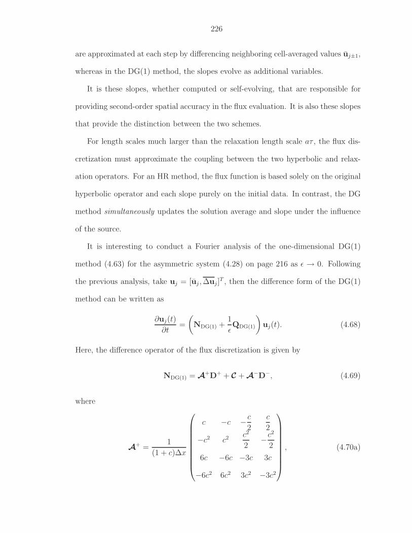
226
are approximated at each step by differencing neighboring cell-averaged values uj±1,
whereas in the DG(1) method, the slopes evolve as additional variables.
It is these slopes, whether computed or self-evolving, that are responsible for
providing second-order spatial accuracy in the flux evaluation. It is also these slopes
that provide the distinction between the two schemes.
For length scales much larger than the relaxation length scale aτ , the flux dis-
cretization must approximate the coupling between the two hyperbolic and relax-
ation operators. For an HR method, the flux function is based solely on the original
hyperbolic operator and each slope purely on the initial data. In contrast, the DG
method simultaneously updates the solution average and slope under the influence
of the source.
It is interesting to conduct a Fourier analysis of the one-dimensional DG(1)
method (4.63) for the asymmetric system (4.28) on page 216 as ǫ → 0. Following
the previous analysis, take uj = [uj , ∆uj ]T , then the difference form of the DG(1)
method can be written as
∂uj(t)
∂t=
(NDG(1) +
1
ǫQDG(1)
)uj(t). (4.68)
Here, the difference operator of the flux discretization is given by
NDG(1) = A+D+ + C + A
−D−, (4.69)
where
A+ =
1
(1 + c)∆x
c −c −c
2
c
2
−c2 c2 c2
2−c2
2
6c −6c −3c 3c
−6c2 6c2 3c2 −3c2
, (4.70a)
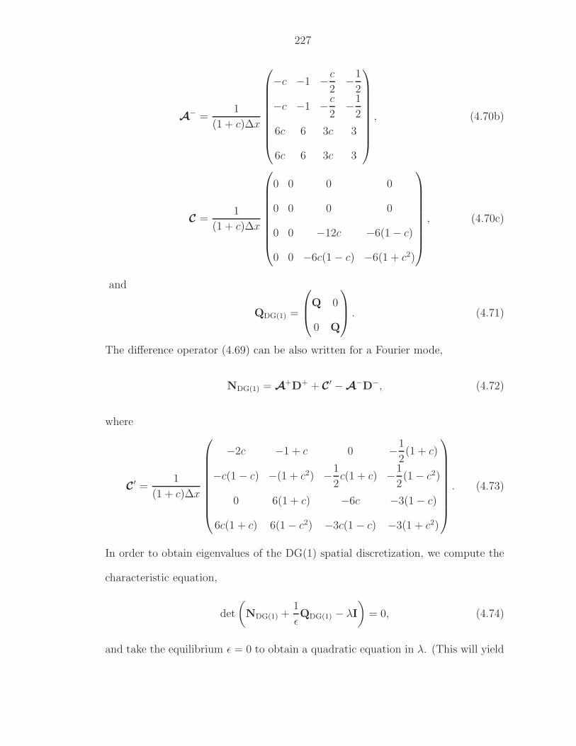
227
A− =
1
(1 + c)∆x
−c −1 −c
2−1
2
−c −1 −c
2−1
2
6c 6 3c 3
6c 6 3c 3
, (4.70b)
C =1
(1 + c)∆x
0 0 0 0
0 0 0 0
0 0 −12c −6(1 − c)
0 0 −6c(1 − c) −6(1 + c2)
, (4.70c)
and
QDG(1) =
Q 0
0 Q
. (4.71)
The difference operator (4.69) can be also written for a Fourier mode,
NDG(1) = A+D+ + C
′ − A−D−, (4.72)
where
C′ =
1
(1 + c)∆x
−2c −1 + c 0 −1
2(1 + c)
−c(1 − c) −(1 + c2) −1
2c(1 + c) −1
2(1 − c2)
0 6(1 + c) −6c −3(1 − c)
6c(1 + c) 6(1 − c2) −3c(1 − c) −3(1 + c2)
. (4.73)
In order to obtain eigenvalues of the DG(1) spatial discretization, we compute the
characteristic equation,
det
(NDG(1) +
1
ǫQDG(1) − λI
)= 0, (4.74)
and take the equilibrium ǫ = 0 to obtain a quadratic equation in λ. (This will yield
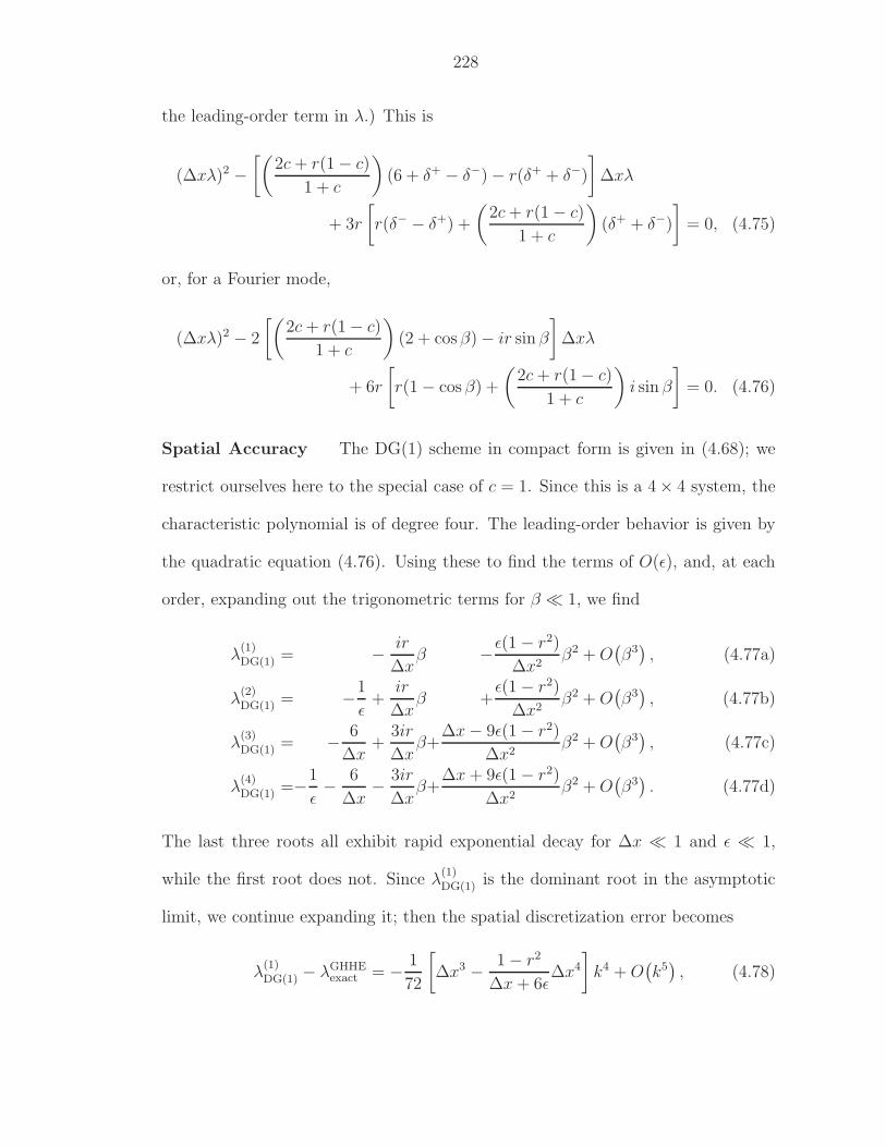
228
the leading-order term in λ.) This is
(∆xλ)2 −[(
2c + r(1 − c)
1 + c
)(6 + δ+ − δ−) − r(δ+ + δ−)
]∆xλ
+ 3r
[r(δ− − δ+) +
(2c + r(1 − c)
1 + c
)(δ+ + δ−)
]= 0, (4.75)
or, for a Fourier mode,
(∆xλ)2 − 2
[(2c + r(1 − c)
1 + c
)(2 + cos β) − ir sin β
]∆xλ
+ 6r
[r(1 − cos β) +
(2c + r(1 − c)
1 + c
)i sin β
]= 0. (4.76)
Spatial Accuracy The DG(1) scheme in compact form is given in (4.68); we
restrict ourselves here to the special case of c = 1. Since this is a 4× 4 system, the
characteristic polynomial is of degree four. The leading-order behavior is given by
the quadratic equation (4.76). Using these to find the terms of O(ǫ), and, at each
order, expanding out the trigonometric terms for β ≪ 1, we find
λ(1)DG(1) = − ir
∆xβ −ǫ(1 − r2)
∆x2β2 + O
(β3), (4.77a)
λ(2)DG(1) = −1
ǫ+
ir
∆xβ +
ǫ(1 − r2)
∆x2β2 + O
(β3), (4.77b)
λ(3)DG(1) = − 6
∆x+
3ir
∆xβ+
∆x − 9ǫ(1 − r2)
∆x2β2 + O
(β3), (4.77c)
λ(4)DG(1) =−1
ǫ− 6
∆x− 3ir
∆xβ+
∆x + 9ǫ(1 − r2)
∆x2β2 + O
(β3). (4.77d)
The last three roots all exhibit rapid exponential decay for ∆x ≪ 1 and ǫ ≪ 1,
while the first root does not. Since λ(1)DG(1) is the dominant root in the asymptotic
limit, we continue expanding it; then the spatial discretization error becomes
λ(1)DG(1) − λGHHE
exact = − 1
72
[∆x3 − 1 − r2
∆x + 6ǫ∆x4
]k4 + O
(k5), (4.78)
229
where we have made the substitution k =β
∆x. Since we are considering the near-
equilibrium limit ǫ ≪ 1, expanding the above error with respect to ǫ provides
λ(1)DG(1)−λGHHE
exact = − 1
72
[r2 ∆x3 + 6ǫ(1 − r2)∆x2 − 36ǫ2(1 − r2)∆x
]k4+O
(ǫ3k4, k5
),
(4.79)
Again, we find a third-order numerical dissipation term independent of ǫ in the
k4-term that can compete with the physical second-order dissipation. The criterion
for the physical dissipation to dominate is
1
72r2∆x3k4 ≪ ǫ(1 − r2)k2. (4.80)
Solving for ∆x leads to the threshold grid size ∆h∗DG(1):
∆x ≪ 2
[9ǫ(1 − r2)
r2k2
]1/3
= 2
(9
rk2 Pe
)1/3
, (4.81)
thus,
∆h∗DG(1) := 2
(9
rk2 Pe
)1/3
, (4.82)
which is a factor of
(9
r2
)1/3
larger than for the HR2 scheme. When rescaled, this is
the same result as Eq. (32) in Lowrie and Morel [LM02, p. 420] which was obtained
from a modified differential-equation analysis.
We directly discretize the advection-diffusion limit (4.27) using the DG(1) scheme
with the Rusanov flux function; this is equivalent to the HLL1 flux with c = 1. The
diffusion term is discretized using the recently developed ‘recovery method’ [vLN05,
vLLvR07]. The eigenvalues of spatial discretization from the Fourier analysis are
λ(1), adv-diffDG(1) − λadv-diff
exact = − r2∆x4
36 [2∆x + 5ǫ(1 − r2)]k4 + O
(k5), (4.83a)
λ(2), adv-diffDG(1) − λadv-diff
exact = − 6
∆x− 15ǫ(1 − r2)
∆x2+ O(k) . (4.83b)
230
The dominant eigenvalue, the first equation, can be further expanded in terms of ǫ
since we are assuming the near-equilibrium limit ǫ ≪ 1; then
λadv-diffDG(1) − λadv-diff
exact = − 1
72
[r2 ∆x3 − 5ǫr2(1 − r2)
2∆x2
]k4 + O
(ǫ2k4, k5
). (4.84)
Again, the dominant numerical dissipation is of precisely the same form as for the
GHHE discretization (4.79).
Finally, we note that, for r = O(ǫ) with ǫ ≪ 1, the DG(1) scheme exhibits
an interesting property. In this case, the fourth-order numerical dissipation term
in (4.79) becomes higher-order in ǫ, and the constraint (4.81) on ∆x is removed.
Thus, the DG(1) scheme should converge with second-order accuracy with ∆x in-
dependent of ǫ, since the higher-even-order terms are too small to compete with
the physical dissipation. This case is included in the diffusive limit considered by
Lowrie and Morel [LM02], and our result agrees with theirs when one accounts for
the time dilation of their scaling.
Spatial-Temporal Accuracy Following the procedure used earlier, the local
truncation error of the DG(1)–MOL combined with the IMEX–SSP2(3,3,2) is found
to have following form:
LTE(1)DG(1)IMEX = −
ir(rν)2
12∆x2
︸ ︷︷ ︸dominant dispersion error
+iǫ r(1 − r2)ν
6∆x
k3
−
r(r − 3(rν)3
)
72∆x3
︸ ︷︷ ︸dominant dissipation error
+ǫ(1 − r2)
12∆x2
k4. (4.85)
Just as for the HR2 method, if the physical dissipation is dominant over the dissi-
pation error,
r(r − 3(rν)3
)
72∆x3k4 ≪ ǫ(1 − r2)k2, (4.86)
231
the method is second-order in space and time. Solving the above equation for ∆x
leads to the threshold grid size:
∆h∗DG(1)IMEX := 2
[9ǫ (1 − r2)
r(r − 3(rν)3
)k2
]1/3
. (4.87)
4.3.4 HR–Hancock Method
It is also interesting to compare the HR2–Hancock method to the DG(1)–Hancock
method. The Hancock methodology is applied to the flux discretization, while a
method for the source term is still to be chosen. Here, similar to the choice for the
DG(1)–Hancock method, we apply the Radau IIA method for the source term. As
described in Chapter II, the update formulas for the cell average are the following:
un+1/3j = un
j − ∆t
3
1
∆x
[fn+1/6j+1/2 − f
n+1/6j−1/2
]+
∆t
3
1
ǫ
[5
4Qu
n+1/3j − 1
4Qun+1
j
], (4.88a)
un+1j = un
j − ∆t
∆x
[fn+1/2j+1/2 − f
n+1/2j−1/2
]+
∆t
ǫ
[3
4Qu
n+1/3j +
1
4Qun+1
j
]. (4.88b)
where u = [u, v]T and the inputs for a Riemann solver are computed by (2.18) on
page 39.
In view of the lengthy expressions, intermediate formulas are omitted, and the
final result for the local truncation error is presented here:
LTEHR2Ha = −
ir (1 − 3ν + 2(rν)2)
12∆x2
︸ ︷︷ ︸dominant dispersion error
+iǫ r(1 − r2)ν
2∆x
k3
−
(1 − r(rν)3 + 2r2ν(ν − 1)
)
8∆x3
︸ ︷︷ ︸dominant dissipation error
−ǫ(1 − r2)(4 + 3ν)
12∆x2
k4. (4.89)
When the grid size is less than the threshold grid size:
∆h∗HR2Ha := 2
[ǫ(1 − r2)
(1 − r(rν)3 + 2r2ν(ν − 1)) k2
]1/3
, (4.90)
232
the physical dissipation dominates over the numerical dissipation under the assump-
tion of near-equilibrium (r = O(1) , ǫ ≪ 1), and the method becomes second-order
in space and time.
4.3.5 DG–Hancock Method
The DG(1)–Hancock method for the 1-D GHHE has the form (4.88) together
with the update equations for ∆uj :
∆un+1/3
j = ∆un
j − ∆t
3
6
∆x
[fn+1/6j+1/2 + f
n+1/6j−1/2 − 2
∆x∆tf(u
n+1/6j )
]
+∆t
3
1
ǫ
[5
4Q∆u
n+1/3
j − 1
4Q∆u
n+1
j
],
(4.91a)
∆un+1
j = ∆un
j − ∆t
∆x6
[fn+1/2j+1/2 + f
n+1/2j−1/2 − 2
∆x∆tf(u
n+1/2j )
]
+∆t
ǫ
[3
4Q∆u
n+1/3
j +1
4Q∆u
n+1
j
].
(4.91b)
After some algebra, the local truncation error of the dominant eigenvalue is found
to be given by
LTE(1)DG(1)Ha = −
[r
72
(r(1 − (rν)2
)2
1 − r2ν− 3rν(1 − ν)
)∆x3
︸ ︷︷ ︸dominant dissipation error
+ǫ (1 − r2)
12(1 − r2ν)2
×(
1 +1
3r2 +
ν2
6
(2r2(r2 − 9) + 3r4ν + r4(9 − 7r2)ν2 + 3r6ν3
))∆x2
]k4. (4.92)
Note that the leading error is a k4-term, hence a dissipation, whereas in other
methods possess a leading dispersion error. The threshold grid size to guarantee
the method be third-order accurate is
∆h∗DG(1)Ha := 2
[9ǫ (1 − r2)(1 − r2ν)
r2(1 − 3ν + (3 + r2)ν2 − 3r2ν3 + (rν)4
)k2
]1/3
. (4.93)
4.3.6 Limiting Flux Function
Here, we show by a Fourier analysis of the semi-discrete HR2–MOL and DG(1)–
MOL methods with the upwind flux based on the frozen wave speeds ±1, that this
233
flux reduces to the Rusanov flux (q = 1) when ǫ → 0 [HSvL05]. Hence, at the
discretization level, solving
∂tu + ∂xv = 0, (4.94a)
∂tv + ∂xu = −1
ǫ(v − ru); Eig(A) = ±1, (4.94b)
by using the upwind flux (also with q = 1 for this system) is identical to directly
solving
∂tu + r∂xu = 0; Eig(A) = r, (4.95)
with the Rusanov flux (q = 1). Note that the genuine upwind flux for the above ad-
vection equation is obtained by q = r. This means that the semi-discrete HR2–MOL
and DG(1)–MOL methods for (4.94) are not strictly upwind in the equilibrium limit
(ǫ → 0).
The dominant dispersion/dissipation errors of semi-discrete methods for advection-
diffusion in the low-frequency limit are given by (3.93) on page 116 for HR2–MOL
and (3.106) on page 121 for DG(1)–MOL with q = 1, while the exact solution for
the GHHE in this case is (4.30).
Consider the DG(1) discretization of the equilibrium advection equation,
∂tu + r∂xu = 0, (4.96)
obtained by taking ǫ = 0 in (4.27):
∂u1,j
∂t= − 1
∆x
[−4f q
j−1/2 − 2f qj+1/2 + 3r(u1,j + u2,j)
], (4.97a)
∂u2,j
∂t= − 1
∆x
[4f q
j+1/2 + 2f qj−1/2 − 3r(u1,j + u2,j)
]. (4.97b)
We substitute for f q a q-flux [vL69], that is,
f qj+1/2(u2,j, u1,j+1) =
r
2(u2,j + u1,j+1) −
q
2(u1,j+1 − u2,j)
=1
2
[2r + (r − q)δ+
]uj +
1
4
[2q + (q − r)δ+
]∆uj . (4.98)
234
In the manner of (4.68), we solve for the characteristic equation of the discrete
system and insert a harmonic modes to find
(∆xλ)2 − 2 [q(2 + cos β) − ir sin β]∆xλ + 6r [r(1 − cos β) + iq sin β] = 0, (4.99)
which is precisely the form of (4.76) on page 228 with
q =2c + r(1 − c)
1 + c. (4.100)
This q corresponds to the first Harten–Lax–Van Leer (HLL1) flux function [HLvL83]
based on the frozen wave speeds aL = |−c| and aR = 1, where
fHLL1(uL, uR) =aL
aR + aL
f(uR) +aR
aR + aL
f(uL) − aRaL
aR + aL
(uR − uL)
=c
1 + cruR +
1
1 + cruL − c
1 + c(uR − uL)
=r
2(uR + uL) − 1
2
2c + r(1 − c)
1 + c(uR − uL), (4.101)
with fL|R = ruL|R. Thus the equilibrium (and near-equilibrium) asymptotic flux
function for the DG(1) scheme applied to the simple one-dimensional problem is
just the HLL1 flux function based on the frozen wave speeds 1 and −c. This
is not completely surprising, as a stable relaxation system has a subcharacteristic
condition, that is, each equilibrium wave speed must be bounded by two frozen wave
speeds [Liu87, CLL94]. Since the upwind flux function in the DG discretization only
knows about the two frozen wave speeds, it continues to use them to approximate
the included equilibrium wave speed. Of course, this means that the equilibrium
method is not strictly upwind.
Note that when the symmetric system (4.25) is considered, the above flux func-
tion reduces to the Rusanov flux:
fRusanov(uL, uR) =r
2(uR + uL) − 1
2(uR − uL). (4.102)

235
Thus, the result of the analysis for the linear advection equation obtained in Chap-
ter III can be directly related here by letting q = 1. This is the reason why we
defined in chapter III the Courant number (3.2) on page 88 based on the frozen
wave speed 1, instead of the equilibrium wave speed r.
4.3.7 Dominant Dispersion/Dissipation Error in 1-D
In summary, the local truncation error of each method is listed for comparison.
semi-discrete methods:
LTEHR2MOL =
[c3
(1 + (rν)2
)+
1
6c3ν
]k3+
[c4
(1
r− 1
3(rν)3
)+
1
6c4
]k4,
(4.103a)
LTE(1)DG(1)MOL =
[c3(rν)2 +
1
6c3ν
]k3+
[1
9c4
(r − 3(rν)3
)+
1
12c4
]k4,
(4.103b)
fully discrete methods:
LTEHR2Ha =
[c3
(1 − 3ν + 2(rν)2
)+
1
2c3ν
]k3
+
[c4
(1
r− (rν)3 + 2rν(ν − 1)
)− 1
12c4 (4 + 3ν)
]k4,
(4.103c)
LTE(1)DG(1)Ha =
[1
9c4
(r(1 − (rν)2
)2
1 − r2ν− 3rν(1 − ν)
)+
c4
12(1 − r2ν)2
×(
1 +1
3r2 +
ν2
6
(2r2(r2 − 9) + 3r4ν + r4(9 − 7r2)ν2 + 3r6ν3
))]
k4,
(4.103d)
where the coefficients of errors attributed to the explicit flux discretization are
c3 = − ir
12∆x2 , c4 = −r
8∆x3 , (4.104a)
and the implicit source-term errors have coefficients
c3 = −iǫr(1 − r2) ∆x , c4 = −ǫ(1 − r2) ∆x2 . (4.104b)
236
The above equations show that HR2–MOL, DG(1)–MOL, and HR2–Hancock have
a first-order error ∼ k3, as c3 = O(ǫ∆x). However, numerically, this error term
is not pronounced in the near-equilibrium limit since ǫ ≪ 1, thus the dominant
error of the methods stem from c3 = O(∆x2). Similarly, the dominant error of
DG(1)–Hancock is c4 = O(∆x3).
As it was described previously, when r = O(ǫ) with ǫ ≪ 1, the DG(1) method
reveals uniform spatial convergence. To demonstrate this, we simply set r = 0, then
the local truncation error of each method becomes
LTEHR2MOL =
[−1
8∆x3 − 1
6ǫ∆x2
]k4, (4.105a)
LTEHR2Ha =
[−1
8∆x3 +
1
12ǫ (4 + 3ν) ∆x2
]k4, (4.105b)
LTE(1)DG(1)MOL = − 1
12ǫ∆x2 k4, (4.105c)
LTE(1)DG(1)Ha = − 1
12ǫ∆x2 k4. (4.105d)
All dispersions, O(k3)-terms, have disappeared, and the dominate error is the dis-
sipation. The dominant dissipation errors of both DG(1) methods are proportional
to ǫ, while HR2 methods have the term,1
8∆x3, which is independent of ǫ. Hence,
DG(1) methods lose their grid size restrictions, but HR2 methods still need to satisfy
the following inequality:
1
8∆x3k4 ≪ ǫk2 −→ ∆x ≪ 2
( ǫ
k2
)1/3
, (4.106)
to guarantee physical dissipation is dominant. Since the leading errors of HR2
methods are proportional to ∆x3, we expect third-order convergence on coarse grids.
4.3.8 Stability of Methods
All four methods described previously include implicit treatment of the source
term. Particularly, an L-stable time integrator is employed. Hence, the stability
237
condition is restricted solely by an explicit discretization of the flux even in the stiff
regime. Recall that, in the near-equilibrium (stiff) regime, discretizing hyperbolic-
relaxation equations with the upwind flux is equivalent to discretizing the advection
equation directly with the Rusanov flux. Thus, it is beneficial to look into the sta-
bility of each method applied to the advection equation. In Chapter III on page 154,
stability analyses of methods with the Rusanov flux was conducted. A rather sur-
prising property was found for the DG(1)–Hancock method; the stability domain
reduces as the equilibrium wave speed gets smaller, while other methods possess
constant stability domains. This property suggests that, in the frozen limit, the
maximum Courant number of the DG(1)–Hancock method is still unity, yet in the
near-equilibrium limit, it will depend on the magnitude of the dimensionless equi-
librium wave speed |r|; the maximum Courant number can be found from (3.162)
on page 155, or Figure 3.15 on page 157.
4.4 Model Equations for Two-Dimensional Problem
In two dimensions we consider the simple system
∂tu + ∂xv + ∂yw = 0, (4.107a)
∂tv + ∂xu + r∂yw = −1
ǫ(v − ru), (4.107b)
∂tw + s∂xv + ∂yu = −1
ǫ(w − su), (4.107c)
where v and w are the fluxes in the x- and y-directions, respectively. The above
equations can be written in vector form:
∂tu(x, t) + ∂xf(u) + ∂yg(u) =1
ǫs(u); x ∈ R
2, t > 0, (4.108)
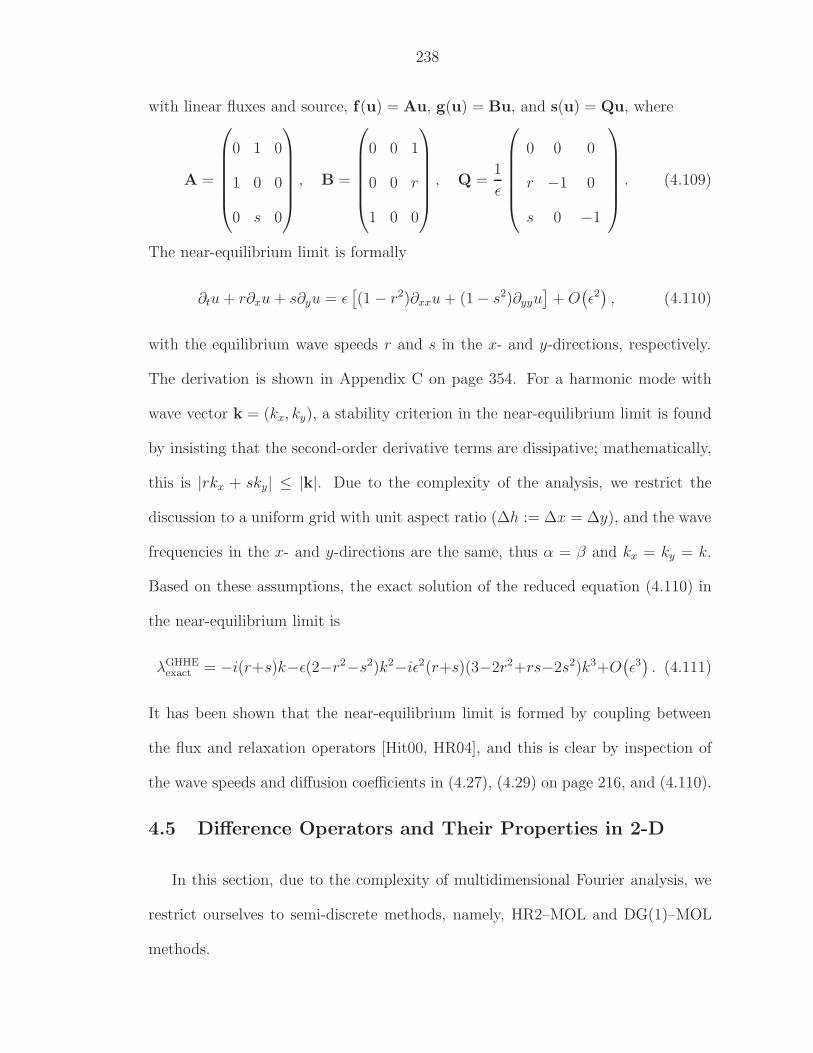
238
with linear fluxes and source, f(u) = Au, g(u) = Bu, and s(u) = Qu, where
A =
0 1 0
1 0 0
0 s 0
, B =
0 0 1
0 0 r
1 0 0
, Q =1
ǫ
0 0 0
r −1 0
s 0 −1
. (4.109)
The near-equilibrium limit is formally
∂tu + r∂xu + s∂yu = ǫ[(1 − r2)∂xxu + (1 − s2)∂yyu
]+ O
(ǫ2), (4.110)
with the equilibrium wave speeds r and s in the x- and y-directions, respectively.
The derivation is shown in Appendix C on page 354. For a harmonic mode with
wave vector k = (kx, ky), a stability criterion in the near-equilibrium limit is found
by insisting that the second-order derivative terms are dissipative; mathematically,
this is |rkx + sky| ≤ |k|. Due to the complexity of the analysis, we restrict the
discussion to a uniform grid with unit aspect ratio (∆h := ∆x = ∆y), and the wave
frequencies in the x- and y-directions are the same, thus α = β and kx = ky = k.
Based on these assumptions, the exact solution of the reduced equation (4.110) in
the near-equilibrium limit is
λGHHEexact = −i(r+s)k−ǫ(2−r2−s2)k2−iǫ2(r+s)(3−2r2+rs−2s2)k3+O
(ǫ3). (4.111)
It has been shown that the near-equilibrium limit is formed by coupling between
the flux and relaxation operators [Hit00, HR04], and this is clear by inspection of
the wave speeds and diffusion coefficients in (4.27), (4.29) on page 216, and (4.110).
4.5 Difference Operators and Their Properties in 2-D
In this section, due to the complexity of multidimensional Fourier analysis, we
restrict ourselves to semi-discrete methods, namely, HR2–MOL and DG(1)–MOL
methods.
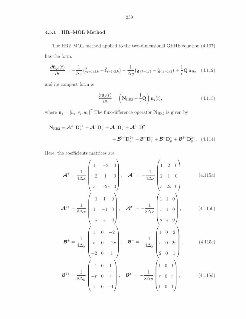
239
4.5.1 HR–MOL Method
The HR2–MOL method applied to the two-dimensional GHHE equation (4.107)
has the form:
∂ujk(t)
∂t= − 1
∆x
(fj+1/2,k − fj−1/2,k
)− 1
∆y
(gj,k+1/2 − gj,k−1/2
)+
1
ǫQujk, (4.112)
and its compact form is
∂uj(t)
∂t=
(NHR2 +
1
ǫQ
)uj(t), (4.113)
where uj = [uj, vj, wj]T The flux-difference operator NHR2 is given by
NHR2 = A2+D2+
x + A+D+
x + A−D−
x + A2−D2−
x
+ B2+D2+
y + B+D+
y + B−D−
y + B2−D2−
y . (4.114)
Here, the coefficients matrices are
A+ =
1
4∆x
1 −2 0
−2 1 0
s −2s 0
, A− = − 1
4∆x
1 2 0
2 1 0
s 2s 0
(4.115a)
A2+ =
1
8∆x
−1 1 0
1 −1 0
−s s 0
, A2− = − 1
8∆x
1 1 0
1 1 0
s s 0
, (4.115b)
B+ =
1
4∆y
1 0 −2
r 0 −2r
−2 0 1
, B− = − 1
4∆y
1 0 2
r 0 2r
2 0 1
, (4.115c)
B2+ =
1
8∆y
−1 0 1
−r 0 r
1 0 −1
, B2− = − 1
8∆y
1 0 1
r 0 r
1 0 1
, (4.115d)
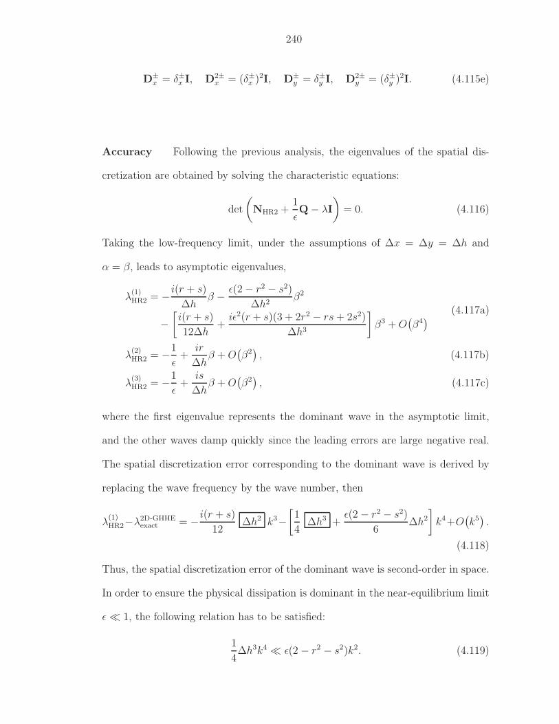
240
D±x = δ±x I, D2±
x = (δ±x )2I, D±y = δ±y I, D2±
y = (δ±y )2I. (4.115e)
Accuracy Following the previous analysis, the eigenvalues of the spatial dis-
cretization are obtained by solving the characteristic equations:
det
(NHR2 +
1
ǫQ − λI
)= 0. (4.116)
Taking the low-frequency limit, under the assumptions of ∆x = ∆y = ∆h and
α = β, leads to asymptotic eigenvalues,
λ(1)HR2 = −i(r + s)
∆hβ − ǫ(2 − r2 − s2)
∆h2β2
−[i(r + s)
12∆h+
iǫ2(r + s)(3 + 2r2 − rs + 2s2)
∆h3
]β3 + O
(β4) (4.117a)
λ(2)HR2 = −1
ǫ+
ir
∆hβ + O
(β2), (4.117b)
λ(3)HR2 = −1
ǫ+
is
∆hβ + O
(β2), (4.117c)
where the first eigenvalue represents the dominant wave in the asymptotic limit,
and the other waves damp quickly since the leading errors are large negative real.
The spatial discretization error corresponding to the dominant wave is derived by
replacing the wave frequency by the wave number, then
λ(1)HR2−λ2D-GHHE
exact = −i(r + s)
12∆h2 k3−
[1
4∆h3 +
ǫ(2 − r2 − s2)
6∆h2
]k4+O
(k5).
(4.118)
Thus, the spatial discretization error of the dominant wave is second-order in space.
In order to ensure the physical dissipation is dominant in the near-equilibrium limit
ǫ ≪ 1, the following relation has to be satisfied:
1
4∆h3k4 ≪ ǫ(2 − r2 − s2)k2. (4.119)
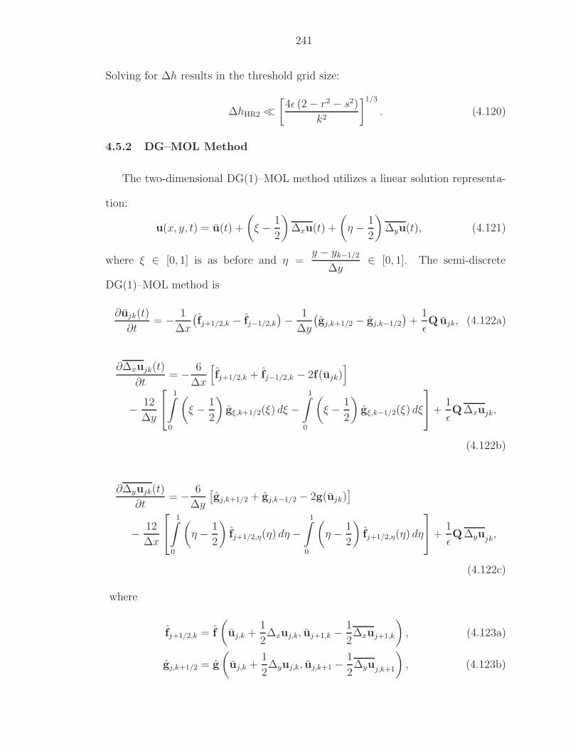
241
Solving for ∆h results in the threshold grid size:
∆hHR2 ≪[4ǫ (2 − r2 − s2)
k2
]1/3
. (4.120)
4.5.2 DG–MOL Method
The two-dimensional DG(1)–MOL method utilizes a linear solution representa-
tion:
u(x, y, t) = u(t) +
(ξ − 1
2
)∆xu(t) +
(η − 1
2
)∆yu(t), (4.121)
where ξ ∈ [0, 1] is as before and η =y − yk−1/2
∆y∈ [0, 1]. The semi-discrete
DG(1)–MOL method is
∂ujk(t)
∂t= − 1
∆x
(fj+1/2,k − fj−1/2,k
)− 1
∆y
(gj,k+1/2 − gj,k−1/2
)+
1
ǫQujk, (4.122a)
∂∆xujk(t)
∂t= − 6
∆x
[fj+1/2,k + fj−1/2,k − 2f(ujk)
]
− 12
∆y
1∫
0
(ξ − 1
2
)gξ,k+1/2(ξ) dξ −
1∫
0
(ξ − 1
2
)gξ,k−1/2(ξ) dξ
+
1
ǫQ∆xujk,
(4.122b)
∂∆yujk(t)
∂t= − 6
∆y
[gj,k+1/2 + gj,k−1/2 − 2g(ujk)
]
− 12
∆x
1∫
0
(η − 1
2
)fj+1/2,η(η) dη −
1∫
0
(η − 1
2
)fj+1/2,η(η) dη
+
1
ǫQ∆yujk,
(4.122c)
where
fj+1/2,k = f
(uj,k +
1
2∆xuj,k, uj+1,k −
1
2∆xuj+1,k
), (4.123a)
gj,k+1/2 = g
(uj,k +
1
2∆yuj,k, uj,k+1 −
1
2∆yuj,k+1
), (4.123b)
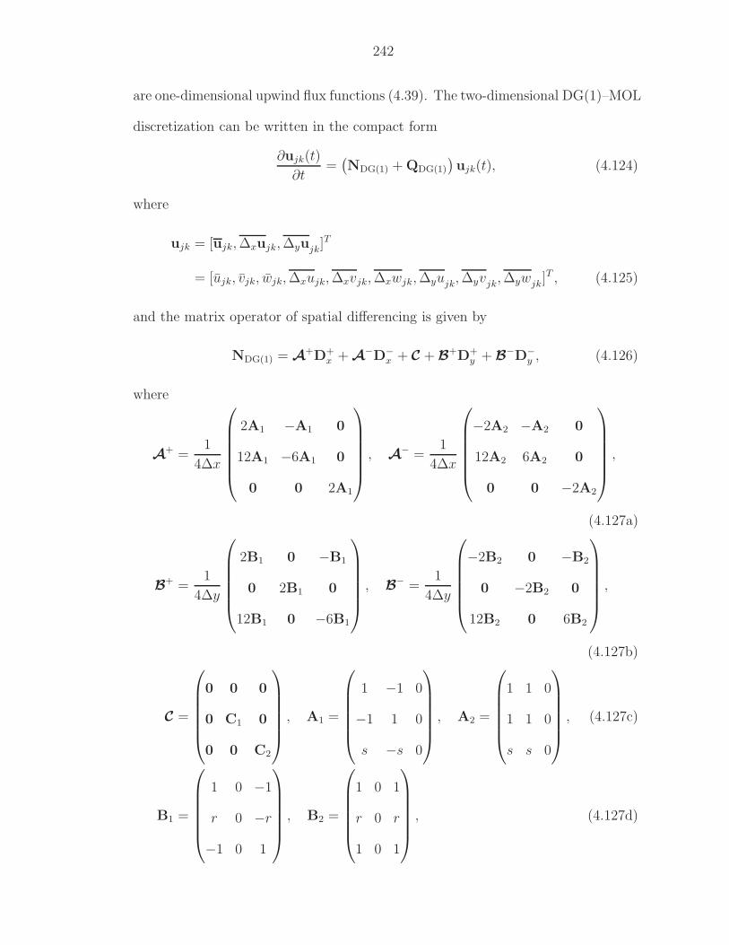
242
are one-dimensional upwind flux functions (4.39). The two-dimensional DG(1)–MOL
discretization can be written in the compact form
∂ujk(t)
∂t=(NDG(1) + QDG(1)
)ujk(t), (4.124)
where
ujk = [ujk, ∆xujk, ∆yujk]T
= [ujk, vjk, wjk, ∆xujk, ∆xvjk, ∆xwjk, ∆yujk, ∆yvjk, ∆ywjk]T , (4.125)
and the matrix operator of spatial differencing is given by
NDG(1) = A+D+
x + A−D−
x + C + B+D+
y + B−D−
y , (4.126)
where
A+ =
1
4∆x
2A1 −A1 0
12A1 −6A1 0
0 0 2A1
, A− =
1
4∆x
−2A2 −A2 0
12A2 6A2 0
0 0 −2A2
,
(4.127a)
B+ =
1
4∆y
2B1 0 −B1
0 2B1 0
12B1 0 −6B1
, B− =
1
4∆y
−2B2 0 −B2
0 −2B2 0
12B2 0 6B2
,
(4.127b)
C =
0 0 0
0 C1 0
0 0 C2
, A1 =
1 −1 0
−1 1 0
s −s 0
, A2 =
1 1 0
1 1 0
s s 0
, (4.127c)
B1 =
1 0 −1
r 0 −r
−1 0 1
, B2 =
1 0 1
r 0 r
1 0 1
, (4.127d)
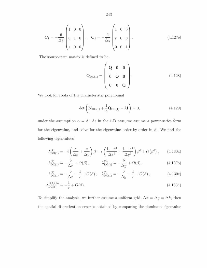
243
C1 = − 6
∆x
1 0 0
0 1 0
s 0 0
, C2 = − 6
∆y
1 0 0
r 0 0
0 0 1
. (4.127e)
The source-term matrix is defined to be
QDG(1) =
Q 0 0
0 Q 0
0 0 Q
. (4.128)
We look for roots of the characteristic polynomial
det
(NDG(1) +
1
ǫQDG(1) − λI
)= 0, (4.129)
under the assumption α = β. As in the 1-D case, we assume a power-series form
for the eigenvalue, and solve for the eigenvalue order-by-order in β. We find the
following eigenvalues:
λ(1)DG(1) = −i
(r
∆x+
s
∆y
)β − ǫ
(1 − r2
∆x2+
1 − s2
∆y2
)β2 + O
(β3), (4.130a)
λ(2)DG(1) = − 6
∆x+ O(β) , λ
(3)DG(1) = − 6
∆y+ O(β) , (4.130b)
λ(4)DG(1) = − 6
∆x− 1
ǫ+ O(β) , λ
(5)DG(1) = − 6
∆y− 1
ǫ+ O(β) , (4.130c)
λ(6,7,8,9)DG(1) = −1
ǫ+ O(β) . (4.130d)
To simplify the analysis, we further assume a uniform grid, ∆x = ∆y = ∆h, then
the spatial-discretization error is obtained by comparing the dominant eigenvalue
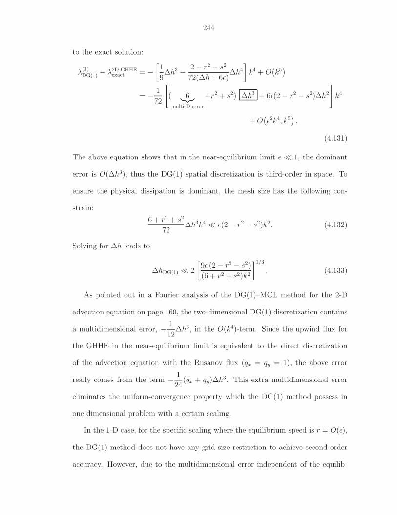
244
to the exact solution:
λ(1)DG(1) − λ2D-GHHE
exact = −[1
9∆h3 − 2 − r2 − s2
72(∆h + 6ǫ)∆h4
]k4 + O
(k5)
= − 1
72
[( 6︸︷︷︸multi-D error
+r2 + s2) ∆h3 + 6ǫ(2 − r2 − s2)∆h2
]k4
+ O(ǫ2k4, k5
).
(4.131)
The above equation shows that in the near-equilibrium limit ǫ ≪ 1, the dominant
error is O(∆h3), thus the DG(1) spatial discretization is third-order in space. To
ensure the physical dissipation is dominant, the mesh size has the following con-
strain:
6 + r2 + s2
72∆h3k4 ≪ ǫ(2 − r2 − s2)k2. (4.132)
Solving for ∆h leads to
∆hDG(1) ≪ 2
[9ǫ (2 − r2 − s2)
(6 + r2 + s2)k2
]1/3
. (4.133)
As pointed out in a Fourier analysis of the DG(1)–MOL method for the 2-D
advection equation on page 169, the two-dimensional DG(1) discretization contains
a multidimensional error, − 1
12∆h3, in the O(k4)-term. Since the upwind flux for
the GHHE in the near-equilibrium limit is equivalent to the direct discretization
of the advection equation with the Rusanov flux (qx = qy = 1), the above error
really comes from the term − 1
24(qx + qy)∆h3. This extra multidimensional error
eliminates the uniform-convergence property which the DG(1) method possess in
one dimensional problem with a certain scaling.
In the 1-D case, for the specific scaling where the equilibrium speed is r = O(ǫ),
the DG(1) method does not have any grid size restriction to achieve second-order
accuracy. However, due to the multidimensional error independent of the equilib-
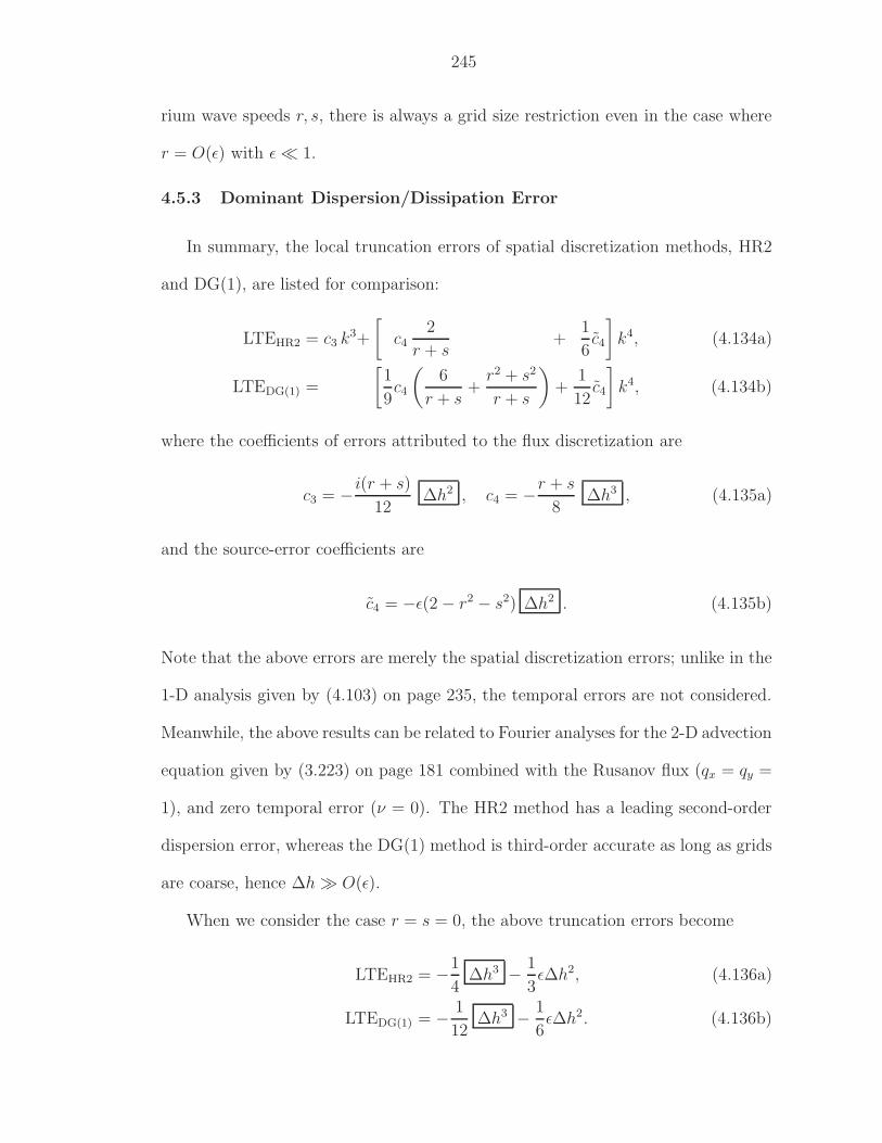
245
rium wave speeds r, s, there is always a grid size restriction even in the case where
r = O(ǫ) with ǫ ≪ 1.
4.5.3 Dominant Dispersion/Dissipation Error
In summary, the local truncation errors of spatial discretization methods, HR2
and DG(1), are listed for comparison:
LTEHR2 = c3 k3+
[c4
2
r + s+
1
6c4
]k4, (4.134a)
LTEDG(1) =
[1
9c4
(6
r + s+
r2 + s2
r + s
)+
1
12c4
]k4, (4.134b)
where the coefficients of errors attributed to the flux discretization are
c3 = −i(r + s)
12∆h2 , c4 = −r + s
8∆h3 , (4.135a)
and the source-error coefficients are
c4 = −ǫ(2 − r2 − s2) ∆h2 . (4.135b)
Note that the above errors are merely the spatial discretization errors; unlike in the
1-D analysis given by (4.103) on page 235, the temporal errors are not considered.
Meanwhile, the above results can be related to Fourier analyses for the 2-D advection
equation given by (3.223) on page 181 combined with the Rusanov flux (qx = qy =
1), and zero temporal error (ν = 0). The HR2 method has a leading second-order
dispersion error, whereas the DG(1) method is third-order accurate as long as grids
are coarse, hence ∆h ≫ O(ǫ).
When we consider the case r = s = 0, the above truncation errors become
LTEHR2 = −1
4∆h3 − 1
3ǫ∆h2, (4.136a)
LTEDG(1) = − 1
12∆h3 − 1
6ǫ∆h2. (4.136b)
246
Unlike in one dimension, the DG(1) method possesses a dominant error independent
to ǫ. Hence, both spatial discretizations yield grid-size restrictions to ensure the
physical dissipation is dominant.
4.5.4 Stability of Methods
Similar to the 1-D case, the stability of the 2-D DG(1)–Hancock method in the
near-equilibrium limit varies as the dimensionless wave speed changes. The stability
limit is given by (3.225) on page 183. The rest of methods remain same stability
properties as the upwind flux; stability limits are listed in Table 3.7 on page 182.
4.6 Grid-Convergence Study in 1-D
4.6.1 Problem Definition
We consider the symmetric model problem (4.25) on page 215. To confirm the
analysis, consider an initial-value problem on a periodic domain with a harmonic
initial condition,
u(x, 0) = ℜu0 exp(ikx) = u0 cos(kx), (4.137)
where k = 2π and u0 = (1, 1)T . A dispersion analysis provides the exact solution for
the computation of the L2-norm [Hit00]. The DG(1)–Hancock method is compared
with the HR2–MOL and DG(1)–MOL methods, both incorporating the IMEX–RK
method [PR05]. For each method, we consider both a frozen limit (ǫ ≫ 1, non-stiff)
and a near-equilibrium limit (ǫ ≪ 1, stiff) with two equilibrium wave speeds in the
stiff regime:
frozen (non-stiff) limit : r =1
2, ǫ = 103, tend = 100, (4.138a)
near-equilibrium (stiff) limit : r = 0,1
2, ǫ = 10−5, tend = 300, (4.138b)
247
and compute the error norms relative to an exact analytic solution. The non-stiff
case represents frozen waves with speed ±1 propagate 100 times over the compu-
tation domain. Similarly, in the stiff case with r =1
2, the equilibrium wave travels
150 wave lengths until tend = 300. Note that r = 0 corresponds to no advection,
hence the system reduces to a pure diffusion equation:
∂tu = ǫ ∂xxu. (4.139)
In both cases, the final analytical damping factor is obtained by
u(tend) = e−ǫ(1−r2)k2 tend ≈ 0.915, (4.140)
thus, a sinusoidal wave is physically dissipated by 8.5%. The Courant numbers
based on the unit wave speed:
νmethod = 1∆t
∆x, (4.141)
are set to be
νHR2–MOL = νHR2–Hancock = 0.9, (4.142a)
νDG(1)–MOL = 0.3, (4.142b)
νDG(1)–Hancock =
0.9 frozen limit
0.3 near-equilibrium limit.
(4.142c)
The DG(1) method requires cell averages uj and slopes ∆uj in each cell for
initial conditions. Given an initial function u(x, 0) in (4.137), the initial cell values
248
are obtained from
uj(t = 0) :=1
∆x
∫
Ij
u(x, 0)dx, (4.143a)
∆xuj(t = 0) :=
∫
Ij
u(x, 0)
(x − xj
∆x
)dx
∫
Ij
(x − xj
∆x
)2
dx
=12
∆x2
∫
Ij
u(x, 0)(x − xj)dx, (4.143b)
where Ij ∈ [xj−1/2, xj+1/2].
4.6.2 Convergence in the Frozen Limit
When the relaxation time is large relative to the residence time, the effect of the
source term is negligible, and the model equations behave like pure advection equa-
tions showed in (4.4) on page 209. The time step based on frozen wave speeds ±1
provides a stable method. Table 4.2 and Figure 4.2 demonstrate second-order con-
vergence in this limit for HR2–IMEX, DG(1)–IMEX, and HR2–Hancock. As we
expected for the DG(1)–Hancock method, third-order convergence is observed. Fig-
ure 4.3 shows the normalized CPU time needed to achieve the target error level.
As in the case of advection, the high accuracy and efficiency of the DG(1)–Hancock
method are evident.
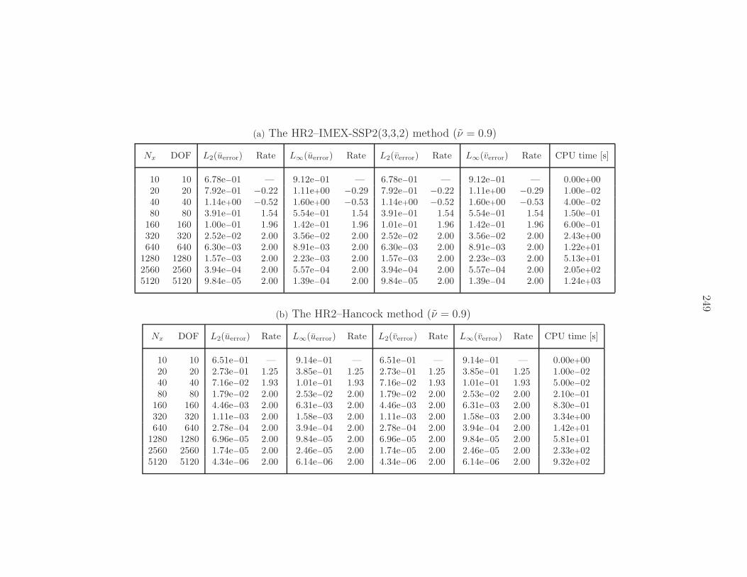
249
(a) The HR2–IMEX-SSP2(3,3,2) method (ν = 0.9)
Nx DOF L2(uerror) Rate L∞(uerror) Rate L2(verror) Rate L∞(verror) Rate CPU time [s]
10 10 6.78e−01 — 9.12e−01 — 6.78e−01 — 9.12e−01 — 0.00e+0020 20 7.92e−01 −0.22 1.11e+00 −0.29 7.92e−01 −0.22 1.11e+00 −0.29 1.00e−0240 40 1.14e+00 −0.52 1.60e+00 −0.53 1.14e+00 −0.52 1.60e+00 −0.53 4.00e−0280 80 3.91e−01 1.54 5.54e−01 1.54 3.91e−01 1.54 5.54e−01 1.54 1.50e−01
160 160 1.00e−01 1.96 1.42e−01 1.96 1.01e−01 1.96 1.42e−01 1.96 6.00e−01320 320 2.52e−02 2.00 3.56e−02 2.00 2.52e−02 2.00 3.56e−02 2.00 2.43e+00640 640 6.30e−03 2.00 8.91e−03 2.00 6.30e−03 2.00 8.91e−03 2.00 1.22e+01
1280 1280 1.57e−03 2.00 2.23e−03 2.00 1.57e−03 2.00 2.23e−03 2.00 5.13e+012560 2560 3.94e−04 2.00 5.57e−04 2.00 3.94e−04 2.00 5.57e−04 2.00 2.05e+025120 5120 9.84e−05 2.00 1.39e−04 2.00 9.84e−05 2.00 1.39e−04 2.00 1.24e+03
(b) The HR2–Hancock method (ν = 0.9)
Nx DOF L2(uerror) Rate L∞(uerror) Rate L2(verror) Rate L∞(verror) Rate CPU time [s]
10 10 6.51e−01 — 9.14e−01 — 6.51e−01 — 9.14e−01 — 0.00e+0020 20 2.73e−01 1.25 3.85e−01 1.25 2.73e−01 1.25 3.85e−01 1.25 1.00e−0240 40 7.16e−02 1.93 1.01e−01 1.93 7.16e−02 1.93 1.01e−01 1.93 5.00e−0280 80 1.79e−02 2.00 2.53e−02 2.00 1.79e−02 2.00 2.53e−02 2.00 2.10e−01
160 160 4.46e−03 2.00 6.31e−03 2.00 4.46e−03 2.00 6.31e−03 2.00 8.30e−01320 320 1.11e−03 2.00 1.58e−03 2.00 1.11e−03 2.00 1.58e−03 2.00 3.34e+00640 640 2.78e−04 2.00 3.94e−04 2.00 2.78e−04 2.00 3.94e−04 2.00 1.42e+01
1280 1280 6.96e−05 2.00 9.84e−05 2.00 6.96e−05 2.00 9.84e−05 2.00 5.81e+012560 2560 1.74e−05 2.00 2.46e−05 2.00 1.74e−05 2.00 2.46e−05 2.00 2.33e+025120 5120 4.34e−06 2.00 6.14e−06 2.00 4.34e−06 2.00 6.14e−06 2.00 9.32e+02
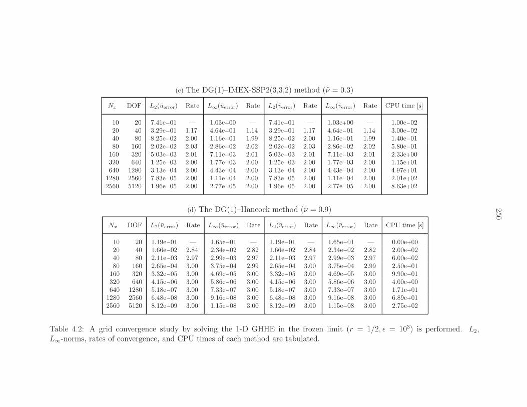
250
(c) The DG(1)–IMEX-SSP2(3,3,2) method (ν = 0.3)
Nx DOF L2(uerror) Rate L∞(uerror) Rate L2(verror) Rate L∞(verror) Rate CPU time [s]
10 20 7.41e−01 — 1.03e+00 — 7.41e−01 — 1.03e+00 — 1.00e−0220 40 3.29e−01 1.17 4.64e−01 1.14 3.29e−01 1.17 4.64e−01 1.14 3.00e−0240 80 8.25e−02 2.00 1.16e−01 1.99 8.25e−02 2.00 1.16e−01 1.99 1.40e−0180 160 2.02e−02 2.03 2.86e−02 2.02 2.02e−02 2.03 2.86e−02 2.02 5.80e−01
160 320 5.03e−03 2.01 7.11e−03 2.01 5.03e−03 2.01 7.11e−03 2.01 2.33e+00320 640 1.25e−03 2.00 1.77e−03 2.00 1.25e−03 2.00 1.77e−03 2.00 1.15e+01640 1280 3.13e−04 2.00 4.43e−04 2.00 3.13e−04 2.00 4.43e−04 2.00 4.97e+01
1280 2560 7.83e−05 2.00 1.11e−04 2.00 7.83e−05 2.00 1.11e−04 2.00 2.01e+022560 5120 1.96e−05 2.00 2.77e−05 2.00 1.96e−05 2.00 2.77e−05 2.00 8.63e+02
(d) The DG(1)–Hancock method (ν = 0.9)
Nx DOF L2(uerror) Rate L∞(uerror) Rate L2(verror) Rate L∞(verror) Rate CPU time [s]
10 20 1.19e−01 — 1.65e−01 — 1.19e−01 — 1.65e−01 — 0.00e+0020 40 1.66e−02 2.84 2.34e−02 2.82 1.66e−02 2.84 2.34e−02 2.82 2.00e−0240 80 2.11e−03 2.97 2.99e−03 2.97 2.11e−03 2.97 2.99e−03 2.97 6.00e−0280 160 2.65e−04 3.00 3.75e−04 2.99 2.65e−04 3.00 3.75e−04 2.99 2.50e−01
160 320 3.32e−05 3.00 4.69e−05 3.00 3.32e−05 3.00 4.69e−05 3.00 9.90e−01320 640 4.15e−06 3.00 5.86e−06 3.00 4.15e−06 3.00 5.86e−06 3.00 4.00e+00640 1280 5.18e−07 3.00 7.33e−07 3.00 5.18e−07 3.00 7.33e−07 3.00 1.71e+01
1280 2560 6.48e−08 3.00 9.16e−08 3.00 6.48e−08 3.00 9.16e−08 3.00 6.89e+012560 5120 8.12e−09 3.00 1.15e−08 3.00 8.12e−09 3.00 1.15e−08 3.00 2.75e+02
Table 4.2: A grid convergence study by solving the 1-D GHHE in the frozen limit (r = 1/2, ǫ = 103) is performed. L2,L∞-norms, rates of convergence, and CPU times of each method are tabulated.
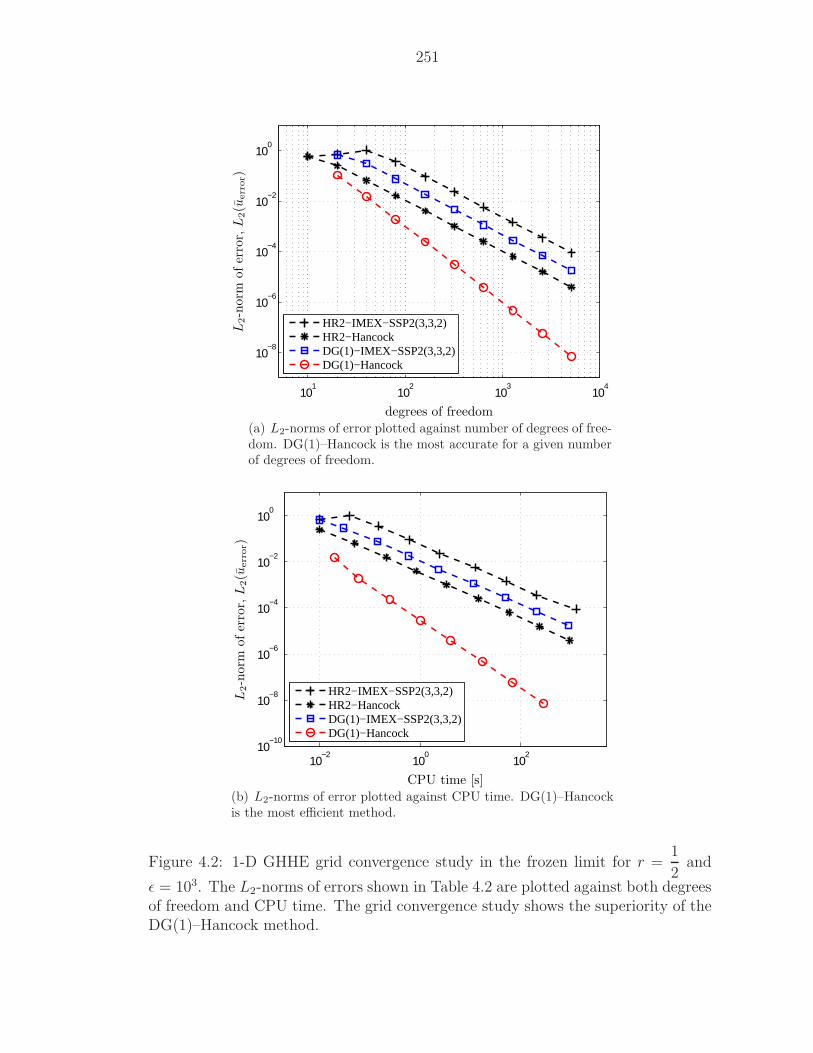
251
101
102
103
104
10−8
10−6
10−4
10−2
100
HR2−IMEX−SSP2(3,3,2)HR2−HancockDG(1)−IMEX−SSP2(3,3,2)DG(1)−Hancock
degrees of freedom
L2-n
orm
ofer
ror,L
2(u
err
or)
(a) L2-norms of error plotted against number of degrees of free-dom. DG(1)–Hancock is the most accurate for a given numberof degrees of freedom.
10−2
100
102
10−10
10−8
10−6
10−4
10−2
100
HR2−IMEX−SSP2(3,3,2)HR2−HancockDG(1)−IMEX−SSP2(3,3,2)DG(1)−Hancock
CPU time [s]
L2-n
orm
ofer
ror,L
2(u
err
or)
(b) L2-norms of error plotted against CPU time. DG(1)–Hancockis the most efficient method.
Figure 4.2: 1-D GHHE grid convergence study in the frozen limit for r =1
2and
ǫ = 103. The L2-norms of errors shown in Table 4.2 are plotted against both degreesof freedom and CPU time. The grid convergence study shows the superiority of theDG(1)–Hancock method.
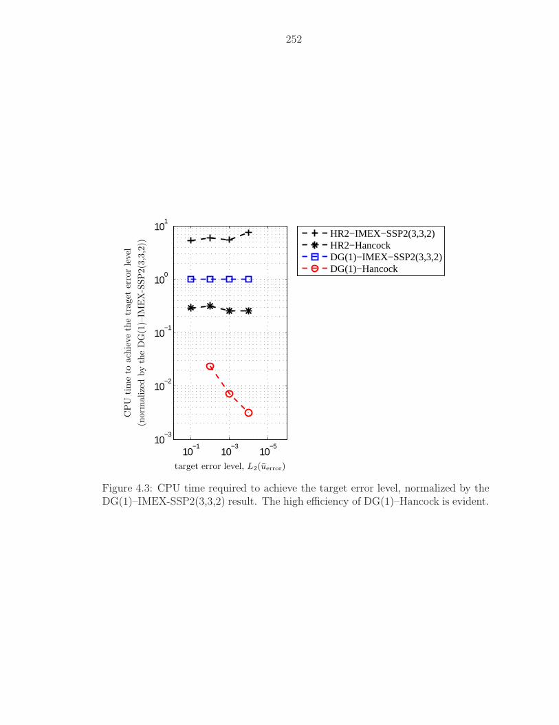
252
10−5
10−3
10−1
10−3
10−2
10−1
100
101
HR2−IMEX−SSP2(3,3,2)HR2−HancockDG(1)−IMEX−SSP2(3,3,2)DG(1)−Hancock
target error level, L2(uerror)
CP
Utim
eto
ach
ieve
the
traget
erro
rle
vel
(norm
alize
dby
the
DG
(1)–
IME
X-S
SP
2(3
,3,2
))
Figure 4.3: CPU time required to achieve the target error level, normalized by theDG(1)–IMEX-SSP2(3,3,2) result. The high efficiency of DG(1)–Hancock is evident.
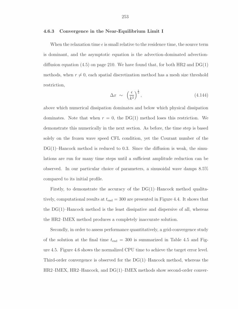
253
4.6.3 Convergence in the Near-Equilibrium Limit I
When the relaxation time ǫ is small relative to the residence time, the source term
is dominant, and the asymptotic equation is the advection-dominated advection-
diffusion equation (4.5) on page 210. We have found that, for both HR2 and DG(1)
methods, when r 6= 0, each spatial discretization method has a mesh size threshold
restriction,
∆x ∼( ǫ
k2
) 13
, (4.144)
above which numerical dissipation dominates and below which physical dissipation
dominates. Note that when r = 0, the DG(1) method loses this restriction. We
demonstrate this numerically in the next section. As before, the time step is based
solely on the frozen wave speed CFL condition, yet the Courant number of the
DG(1)–Hancock method is reduced to 0.3. Since the diffusion is weak, the simu-
lations are run for many time steps until a sufficient amplitude reduction can be
observed. In our particular choice of parameters, a sinusoidal wave damps 8.5%
compared to its initial profile.
Firstly, to demonstrate the accuracy of the DG(1)–Hancock method qualita-
tively, computational results at tend = 300 are presented in Figure 4.4. It shows that
the DG(1)–Hancock method is the least dissipative and dispersive of all, whereas
the HR2–IMEX method produces a completely inaccurate solution.
Secondly, in order to assess performance quantitatively, a grid-convergence study
of the solution at the final time tend = 300 is summarized in Table 4.5 and Fig-
ure 4.5. Figure 4.6 shows the normalized CPU time to achieve the target error level.
Third-order convergence is observed for the DG(1)–Hancock method, whereas the
HR2–IMEX, HR2–Hancock, and DG(1)–IMEX methods show second-order conver-
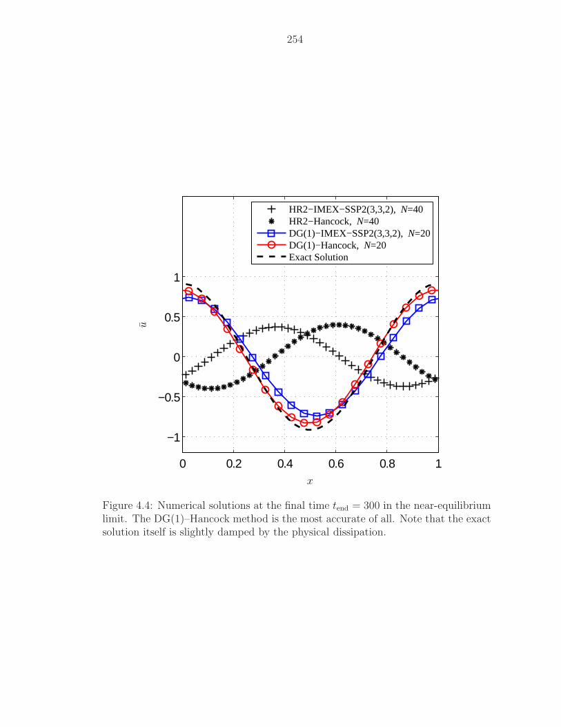
254
0 0.2 0.4 0.6 0.8 1
−1
−0.5
0
0.5
1
HR2−IMEX−SSP2(3,3,2), N=40HR2−Hancock, N=40DG(1)−IMEX−SSP2(3,3,2), N=20DG(1)−Hancock, N=20Exact Solution
x
u
Figure 4.4: Numerical solutions at the final time tend = 300 in the near-equilibriumlimit. The DG(1)–Hancock method is the most accurate of all. Note that the exactsolution itself is slightly damped by the physical dissipation.
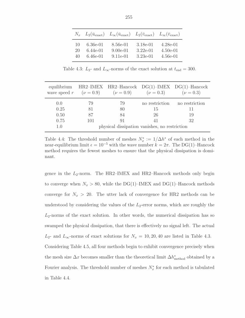
255
Nx L2(uexact) L∞(uexact) L2(vexact) L∞(vexact)
10 6.36e-01 8.56e-01 3.18e-01 4.28e-0120 6.44e-01 9.00e-01 3.22e-01 4.50e-0140 6.46e-01 9.11e-01 3.23e-01 4.56e-01
Table 4.3: L2- and L∞-norms of the exact solution at tend = 300.
equilibrium HR2–IMEX HR2–Hancock DG(1)–IMEX DG(1)–Hancockwave speed r (ν = 0.9) (ν = 0.9) (ν = 0.3) (ν = 0.3)
0.0 79 79 no restriction no restriction0.25 81 80 15 110.50 87 84 26 190.75 101 91 41 321.0 physical dissipation vanishes, no restriction
Table 4.4: The threshold number of meshes N∗x := 1/∆h∗ of each method in the
near-equilibrium limit ǫ = 10−5 with the wave number k = 2π. The DG(1)–Hancockmethod requires the fewest meshes to ensure that the physical dissipation is domi-nant.
gence in the L2-norm. The HR2–IMEX and HR2–Hancock methods only begin
to converge when Nx > 80, while the DG(1)–IMEX and DG(1)–Hancock methods
converge for Nx > 20. The utter lack of convergence for HR2 methods can be
understood by considering the values of the L2-error norms, which are roughly the
L2-norms of the exact solution. In other words, the numerical dissipation has so
swamped the physical dissipation, that there is effectively no signal left. The actual
L2- and L∞-norms of exact solutions for Nx = 10, 20, 40 are listed in Table 4.3.
Considering Table 4.5, all four methods begin to exhibit convergence precisely when
the mesh size ∆x becomes smaller than the theoretical limit ∆h∗method obtained by a
Fourier analysis. The threshold number of meshes N∗x for each method is tabulated
in Table 4.4.
256
As for DG(1) methods, we observe that the order of accuracy seem to decrease
on finer grids. This can be understood by the Fourier analysis given in (4.103).
For instance, the DG(1)–MOL has two leading dispersion errors: c3 ∝ ∆x2 and
c3 ∝ ǫ∆x. On coarse grids, hence c3 ≫ c3, second-order convergence is pronounced.
However, as grids get finder and start resolving the relaxation scale, these two
coefficients become comparable, and eventually the first-order error, c3, dominates.
A similar observation can be made for the DG(1)–Hancock method regarding its
convergence reduction from third- to second-order.
Lastly, it can be observed that the HR2–Hancock method in this limit loses the
high accurate observed in the frozen limit. The reason is that the shift condition of
the HR2–Hancock method owing to the upwind flux is no longer preserved in the
near-equilibrium limit. Note that in this limit the flux becomes the Rusanov/HLL1
type (on page 234); excessive numerical dissipation reduces the accuracy to almost
the same level as for the HR2–IMEX method.
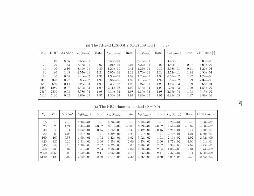
257
(a) The HR2–IMEX-SSP2(3,3,2) method (ν = 0.9)
Nx DOF ∆x/∆h⋆ L2(uerror) Rate L∞(uerror) Rate L2(verror) Rate L∞(verror) Rate CPU time [s]
10 10 8.65 6.36e−01 — 8.56e−01 — 3.18e−01 — 4.28e−01 — 0.00e+0020 20 4.33 6.45e−01 −0.02 9.01e−01 −0.07 3.22e−01 −0.02 4.50e−01 −0.07 3.00e−0240 40 2.16 8.46e−01 −0.39 1.20e+00 −0.41 4.23e−01 −0.39 5.98e−01 −0.41 1.20e−0180 80 1.08 3.57e−01 1.24 5.05e−01 1.24 1.79e−01 1.24 2.52e−01 1.24 4.50e−01
160 160 0.54 9.40e−02 1.93 1.33e−01 1.92 4.70e−02 1.93 6.65e−02 1.92 1.79e+00320 320 0.27 2.36e−02 1.99 3.34e−02 1.99 1.18e−02 1.99 1.67e−02 1.99 7.37e+00640 640 0.14 5.93e−03 1.99 8.39e−03 1.99 2.97e−03 1.99 4.19e−03 1.99 3.64e+01
1280 1280 0.07 1.49e−03 1.99 2.11e−03 1.99 7.46e−04 1.99 1.06e−03 1.99 1.53e+022560 2560 0.03 3.78e−04 1.98 5.34e−04 1.98 1.89e−04 1.98 2.67e−04 1.98 6.13e+025120 5120 0.02 9.64e−05 1.97 1.36e−04 1.97 4.82e−05 1.97 6.81e−05 1.97 3.89e+03
(b) The HR2–Hancock method (ν = 0.9)
Nx DOF ∆x/∆h⋆ L2(uerror) Rate L∞(uerror) Rate L2(verror) Rate L∞(verror) Rate CPU time [s]
10 10 8.43 6.36e−01 — 8.56e−01 — 3.18e−01 — 4.28e−01 — 1.00e−0220 20 4.21 6.45e−01 −0.02 9.01e−01 −0.07 3.23e−01 −0.02 4.51e−01 −0.07 4.00e−0240 40 2.11 8.83e−01 −0.45 1.25e+00 −0.47 4.42e−01 −0.45 6.24e−01 −0.47 1.60e−0180 80 1.05 3.81e−01 1.21 5.39e−01 1.21 1.91e−01 1.21 2.70e−01 1.21 6.30e−01
160 160 0.53 1.00e−01 1.93 1.42e−01 1.92 5.02e−02 1.93 7.10e−02 1.92 2.52e+00320 320 0.26 2.51e−02 2.00 3.55e−02 2.00 1.25e−02 2.00 1.77e−02 2.00 1.01e+01640 640 0.13 6.20e−03 2.02 8.77e−03 2.02 3.10e−03 2.02 4.38e−03 2.02 4.25e+01
1280 1280 0.07 1.51e−03 2.04 2.13e−03 2.04 7.53e−04 2.04 1.06e−03 2.04 1.74e+022560 2560 0.03 3.50e−04 2.11 4.95e−04 2.11 1.75e−04 2.11 2.47e−04 2.11 6.98e+025120 5120 0.02 7.12e−05 2.30 1.01e−04 2.30 3.56e−05 2.30 5.04e−05 2.30 2.85e+03
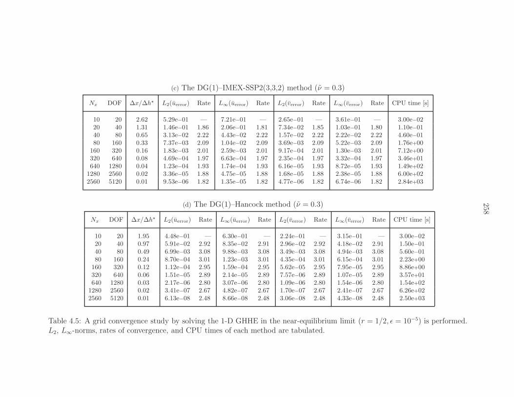
258
(c) The DG(1)–IMEX-SSP2(3,3,2) method (ν = 0.3)
Nx DOF ∆x/∆h⋆ L2(uerror) Rate L∞(uerror) Rate L2(verror) Rate L∞(verror) Rate CPU time [s]
10 20 2.62 5.29e−01 — 7.21e−01 — 2.65e−01 — 3.61e−01 — 3.00e−0220 40 1.31 1.46e−01 1.86 2.06e−01 1.81 7.34e−02 1.85 1.03e−01 1.80 1.10e−0140 80 0.65 3.13e−02 2.22 4.43e−02 2.22 1.57e−02 2.22 2.22e−02 2.22 4.60e−0180 160 0.33 7.37e−03 2.09 1.04e−02 2.09 3.69e−03 2.09 5.22e−03 2.09 1.76e+00
160 320 0.16 1.83e−03 2.01 2.59e−03 2.01 9.17e−04 2.01 1.30e−03 2.01 7.12e+00320 640 0.08 4.69e−04 1.97 6.63e−04 1.97 2.35e−04 1.97 3.32e−04 1.97 3.46e+01640 1280 0.04 1.23e−04 1.93 1.74e−04 1.93 6.16e−05 1.93 8.72e−05 1.93 1.49e+02
1280 2560 0.02 3.36e−05 1.88 4.75e−05 1.88 1.68e−05 1.88 2.38e−05 1.88 6.00e+022560 5120 0.01 9.53e−06 1.82 1.35e−05 1.82 4.77e−06 1.82 6.74e−06 1.82 2.84e+03
(d) The DG(1)–Hancock method (ν = 0.3)
Nx DOF ∆x/∆h⋆ L2(uerror) Rate L∞(uerror) Rate L2(verror) Rate L∞(verror) Rate CPU time [s]
10 20 1.95 4.48e−01 — 6.30e−01 — 2.24e−01 — 3.15e−01 — 3.00e−0220 40 0.97 5.91e−02 2.92 8.35e−02 2.91 2.96e−02 2.92 4.18e−02 2.91 1.50e−0140 80 0.49 6.99e−03 3.08 9.88e−03 3.08 3.49e−03 3.08 4.94e−03 3.08 5.60e−0180 160 0.24 8.70e−04 3.01 1.23e−03 3.01 4.35e−04 3.01 6.15e−04 3.01 2.23e+00
160 320 0.12 1.12e−04 2.95 1.59e−04 2.95 5.62e−05 2.95 7.95e−05 2.95 8.86e+00320 640 0.06 1.51e−05 2.89 2.14e−05 2.89 7.57e−06 2.89 1.07e−05 2.89 3.57e+01640 1280 0.03 2.17e−06 2.80 3.07e−06 2.80 1.09e−06 2.80 1.54e−06 2.80 1.54e+02
1280 2560 0.02 3.41e−07 2.67 4.82e−07 2.67 1.70e−07 2.67 2.41e−07 2.67 6.26e+022560 5120 0.01 6.13e−08 2.48 8.66e−08 2.48 3.06e−08 2.48 4.33e−08 2.48 2.50e+03
Table 4.5: A grid convergence study by solving the 1-D GHHE in the near-equilibrium limit (r = 1/2, ǫ = 10−5) is performed.L2, L∞-norms, rates of convergence, and CPU times of each method are tabulated.
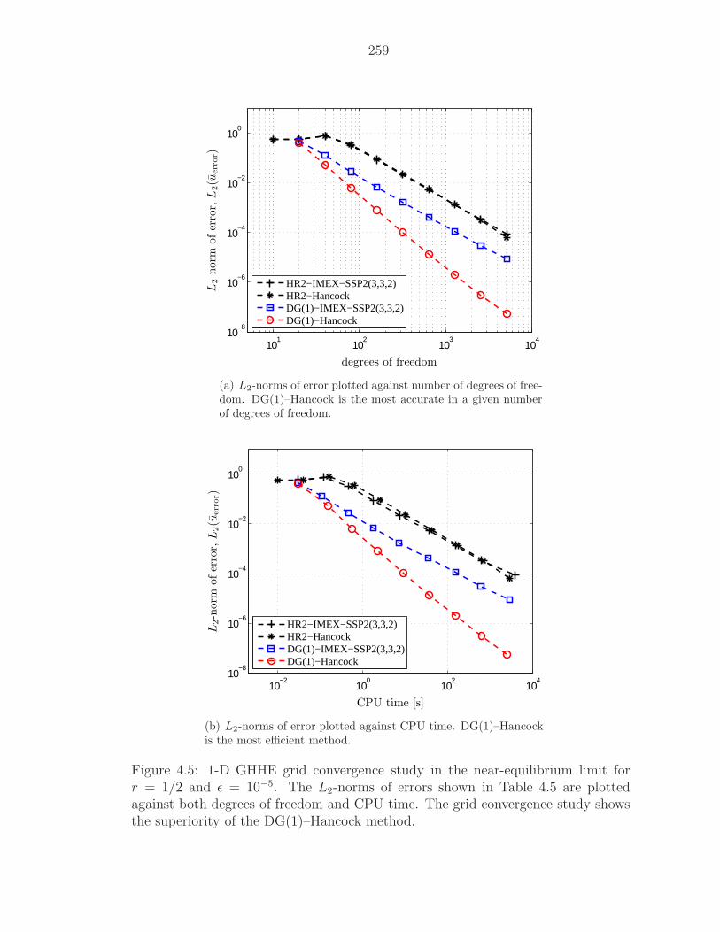
259
101
102
103
104
10−8
10−6
10−4
10−2
100
HR2−IMEX−SSP2(3,3,2)HR2−HancockDG(1)−IMEX−SSP2(3,3,2)DG(1)−Hancock
degrees of freedom
L2-n
orm
ofer
ror,L
2(u
err
or)
(a) L2-norms of error plotted against number of degrees of free-dom. DG(1)–Hancock is the most accurate in a given numberof degrees of freedom.
10−2
100
102
104
10−8
10−6
10−4
10−2
100
HR2−IMEX−SSP2(3,3,2)HR2−HancockDG(1)−IMEX−SSP2(3,3,2)DG(1)−Hancock
CPU time [s]
L2-n
orm
ofer
ror,L
2(u
err
or)
(b) L2-norms of error plotted against CPU time. DG(1)–Hancockis the most efficient method.
Figure 4.5: 1-D GHHE grid convergence study in the near-equilibrium limit forr = 1/2 and ǫ = 10−5. The L2-norms of errors shown in Table 4.5 are plottedagainst both degrees of freedom and CPU time. The grid convergence study showsthe superiority of the DG(1)–Hancock method.
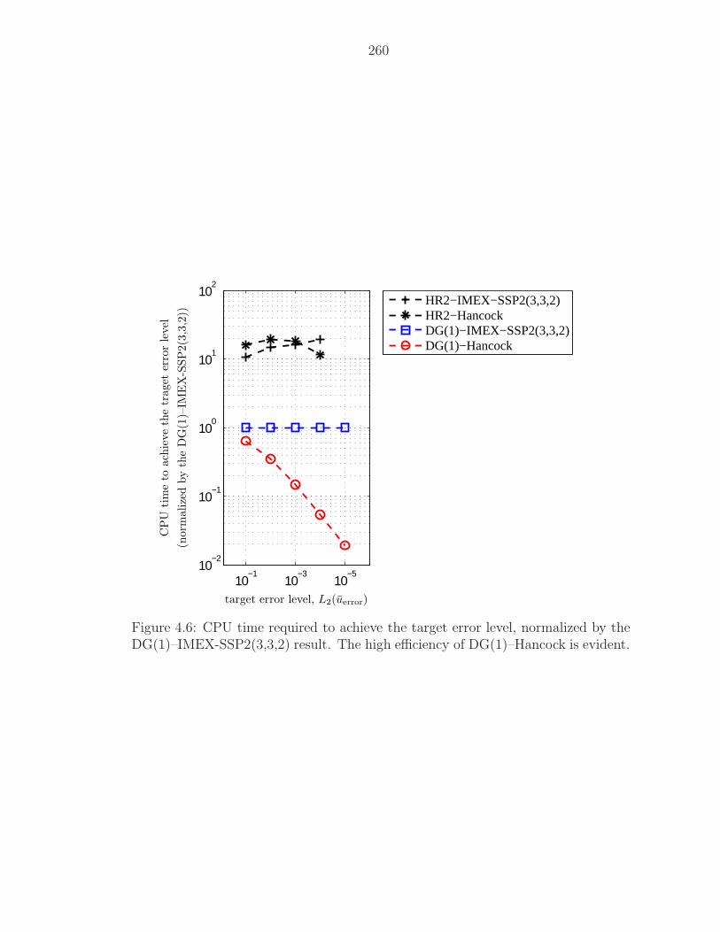
260
10−5
10−3
10−1
10−2
10−1
100
101
102
HR2−IMEX−SSP2(3,3,2)HR2−HancockDG(1)−IMEX−SSP2(3,3,2)DG(1)−Hancock
target error level, L2(uerror)
CP
Utim
eto
ach
ieve
the
traget
erro
rle
vel
(norm
alize
dby
the
DG
(1)–
IME
X-S
SP
2(3
,3,2
))
Figure 4.6: CPU time required to achieve the target error level, normalized by theDG(1)–IMEX-SSP2(3,3,2) result. The high efficiency of DG(1)–Hancock is evident.
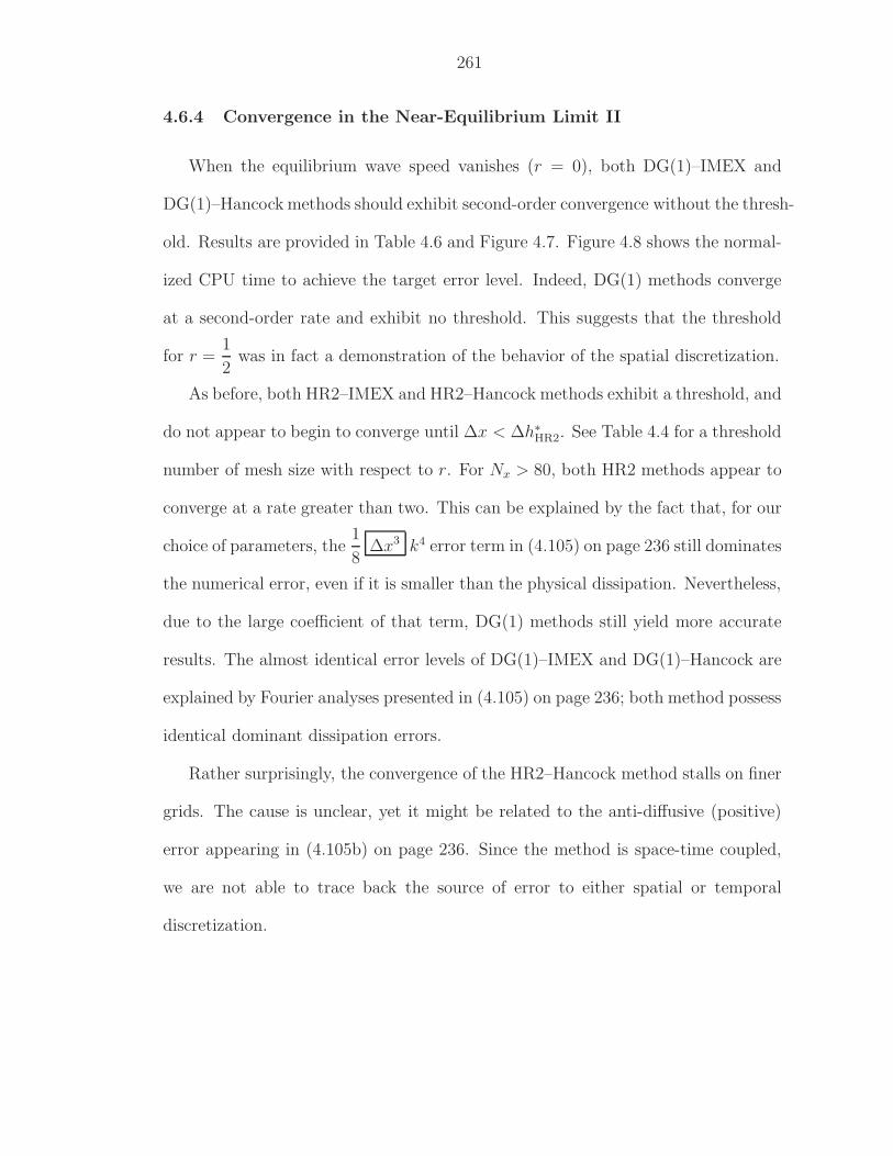
261
4.6.4 Convergence in the Near-Equilibrium Limit II
When the equilibrium wave speed vanishes (r = 0), both DG(1)–IMEX and
DG(1)–Hancock methods should exhibit second-order convergence without the thresh-
old. Results are provided in Table 4.6 and Figure 4.7. Figure 4.8 shows the normal-
ized CPU time to achieve the target error level. Indeed, DG(1) methods converge
at a second-order rate and exhibit no threshold. This suggests that the threshold
for r =1
2was in fact a demonstration of the behavior of the spatial discretization.
As before, both HR2–IMEX and HR2–Hancock methods exhibit a threshold, and
do not appear to begin to converge until ∆x < ∆h∗HR2. See Table 4.4 for a threshold
number of mesh size with respect to r. For Nx > 80, both HR2 methods appear to
converge at a rate greater than two. This can be explained by the fact that, for our
choice of parameters, the1
8∆x3 k4 error term in (4.105) on page 236 still dominates
the numerical error, even if it is smaller than the physical dissipation. Nevertheless,
due to the large coefficient of that term, DG(1) methods still yield more accurate
results. The almost identical error levels of DG(1)–IMEX and DG(1)–Hancock are
explained by Fourier analyses presented in (4.105) on page 236; both method possess
identical dominant dissipation errors.
Rather surprisingly, the convergence of the HR2–Hancock method stalls on finer
grids. The cause is unclear, yet it might be related to the anti-diffusive (positive)
error appearing in (4.105b) on page 236. Since the method is space-time coupled,
we are not able to trace back the source of error to either spatial or temporal
discretization.
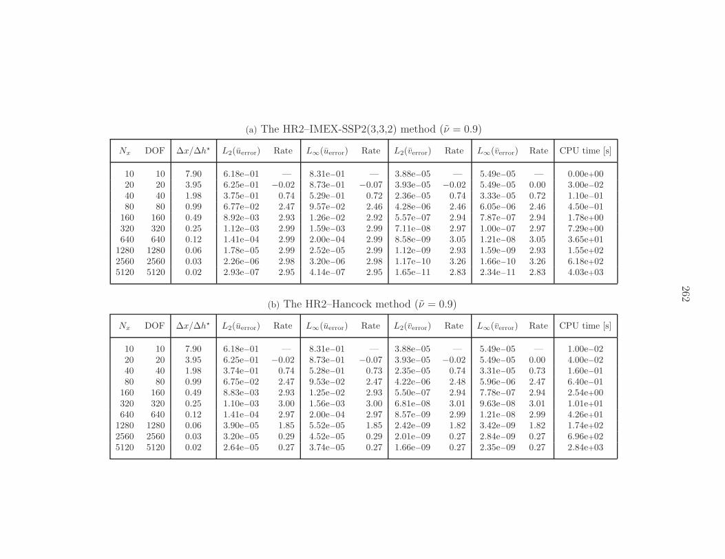
262
(a) The HR2–IMEX-SSP2(3,3,2) method (ν = 0.9)
Nx DOF ∆x/∆h⋆ L2(uerror) Rate L∞(uerror) Rate L2(verror) Rate L∞(verror) Rate CPU time [s]
10 10 7.90 6.18e−01 — 8.31e−01 — 3.88e−05 — 5.49e−05 — 0.00e+0020 20 3.95 6.25e−01 −0.02 8.73e−01 −0.07 3.93e−05 −0.02 5.49e−05 0.00 3.00e−0240 40 1.98 3.75e−01 0.74 5.29e−01 0.72 2.36e−05 0.74 3.33e−05 0.72 1.10e−0180 80 0.99 6.77e−02 2.47 9.57e−02 2.46 4.28e−06 2.46 6.05e−06 2.46 4.50e−01
160 160 0.49 8.92e−03 2.93 1.26e−02 2.92 5.57e−07 2.94 7.87e−07 2.94 1.78e+00320 320 0.25 1.12e−03 2.99 1.59e−03 2.99 7.11e−08 2.97 1.00e−07 2.97 7.29e+00640 640 0.12 1.41e−04 2.99 2.00e−04 2.99 8.58e−09 3.05 1.21e−08 3.05 3.65e+01
1280 1280 0.06 1.78e−05 2.99 2.52e−05 2.99 1.12e−09 2.93 1.59e−09 2.93 1.55e+022560 2560 0.03 2.26e−06 2.98 3.20e−06 2.98 1.17e−10 3.26 1.66e−10 3.26 6.18e+025120 5120 0.02 2.93e−07 2.95 4.14e−07 2.95 1.65e−11 2.83 2.34e−11 2.83 4.03e+03
(b) The HR2–Hancock method (ν = 0.9)
Nx DOF ∆x/∆h⋆ L2(uerror) Rate L∞(uerror) Rate L2(verror) Rate L∞(verror) Rate CPU time [s]
10 10 7.90 6.18e−01 — 8.31e−01 — 3.88e−05 — 5.49e−05 — 1.00e−0220 20 3.95 6.25e−01 −0.02 8.73e−01 −0.07 3.93e−05 −0.02 5.49e−05 0.00 4.00e−0240 40 1.98 3.74e−01 0.74 5.28e−01 0.73 2.35e−05 0.74 3.31e−05 0.73 1.60e−0180 80 0.99 6.75e−02 2.47 9.53e−02 2.47 4.22e−06 2.48 5.96e−06 2.47 6.40e−01
160 160 0.49 8.83e−03 2.93 1.25e−02 2.93 5.50e−07 2.94 7.78e−07 2.94 2.54e+00320 320 0.25 1.10e−03 3.00 1.56e−03 3.00 6.81e−08 3.01 9.63e−08 3.01 1.01e+01640 640 0.12 1.41e−04 2.97 2.00e−04 2.97 8.57e−09 2.99 1.21e−08 2.99 4.26e+01
1280 1280 0.06 3.90e−05 1.85 5.52e−05 1.85 2.42e−09 1.82 3.42e−09 1.82 1.74e+022560 2560 0.03 3.20e−05 0.29 4.52e−05 0.29 2.01e−09 0.27 2.84e−09 0.27 6.96e+025120 5120 0.02 2.64e−05 0.27 3.74e−05 0.27 1.66e−09 0.27 2.35e−09 0.27 2.84e+03
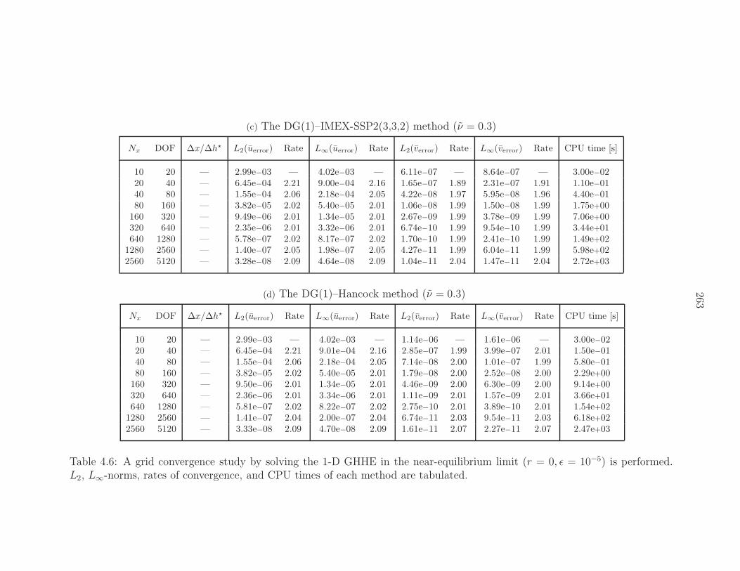
263
(c) The DG(1)–IMEX-SSP2(3,3,2) method (ν = 0.3)
Nx DOF ∆x/∆h⋆ L2(uerror) Rate L∞(uerror) Rate L2(verror) Rate L∞(verror) Rate CPU time [s]
10 20 — 2.99e−03 — 4.02e−03 — 6.11e−07 — 8.64e−07 — 3.00e−0220 40 — 6.45e−04 2.21 9.00e−04 2.16 1.65e−07 1.89 2.31e−07 1.91 1.10e−0140 80 — 1.55e−04 2.06 2.18e−04 2.05 4.22e−08 1.97 5.95e−08 1.96 4.40e−0180 160 — 3.82e−05 2.02 5.40e−05 2.01 1.06e−08 1.99 1.50e−08 1.99 1.75e+00
160 320 — 9.49e−06 2.01 1.34e−05 2.01 2.67e−09 1.99 3.78e−09 1.99 7.06e+00320 640 — 2.35e−06 2.01 3.32e−06 2.01 6.74e−10 1.99 9.54e−10 1.99 3.44e+01640 1280 — 5.78e−07 2.02 8.17e−07 2.02 1.70e−10 1.99 2.41e−10 1.99 1.49e+02
1280 2560 — 1.40e−07 2.05 1.98e−07 2.05 4.27e−11 1.99 6.04e−11 1.99 5.98e+022560 5120 — 3.28e−08 2.09 4.64e−08 2.09 1.04e−11 2.04 1.47e−11 2.04 2.72e+03
(d) The DG(1)–Hancock method (ν = 0.3)
Nx DOF ∆x/∆h⋆ L2(uerror) Rate L∞(uerror) Rate L2(verror) Rate L∞(verror) Rate CPU time [s]
10 20 — 2.99e−03 — 4.02e−03 — 1.14e−06 — 1.61e−06 — 3.00e−0220 40 — 6.45e−04 2.21 9.01e−04 2.16 2.85e−07 1.99 3.99e−07 2.01 1.50e−0140 80 — 1.55e−04 2.06 2.18e−04 2.05 7.14e−08 2.00 1.01e−07 1.99 5.80e−0180 160 — 3.82e−05 2.02 5.40e−05 2.01 1.79e−08 2.00 2.52e−08 2.00 2.29e+00
160 320 — 9.50e−06 2.01 1.34e−05 2.01 4.46e−09 2.00 6.30e−09 2.00 9.14e+00320 640 — 2.36e−06 2.01 3.34e−06 2.01 1.11e−09 2.01 1.57e−09 2.01 3.66e+01640 1280 — 5.81e−07 2.02 8.22e−07 2.02 2.75e−10 2.01 3.89e−10 2.01 1.54e+02
1280 2560 — 1.41e−07 2.04 2.00e−07 2.04 6.74e−11 2.03 9.54e−11 2.03 6.18e+022560 5120 — 3.33e−08 2.09 4.70e−08 2.09 1.61e−11 2.07 2.27e−11 2.07 2.47e+03
Table 4.6: A grid convergence study by solving the 1-D GHHE in the near-equilibrium limit (r = 0, ǫ = 10−5) is performed.L2, L∞-norms, rates of convergence, and CPU times of each method are tabulated.
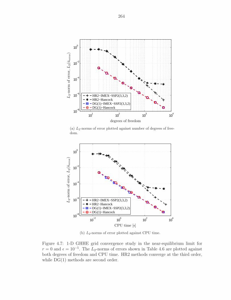
264
101
102
103
104
10−8
10−6
10−4
10−2
100
HR2−IMEX−SSP2(3,3,2)HR2−HancockDG(1)−IMEX−SSP2(3,3,2)DG(1)−Hancock
degrees of freedom
L2-n
orm
ofer
ror,L
2(u
err
or)
(a) L2-norms of error plotted against number of degrees of free-dom.
10−2
100
102
104
10−8
10−6
10−4
10−2
100
HR2−IMEX−SSP2(3,3,2)HR2−HancockDG(1)−IMEX−SSP2(3,3,2)DG(1)−Hancock
CPU time [s]
L2-n
orm
ofer
ror,L
2(u
err
or)
(b) L2-norms of error plotted against CPU time.
Figure 4.7: 1-D GHHE grid convergence study in the near-equilibrium limit forr = 0 and ǫ = 10−5. The L2-norms of errors shown in Table 4.6 are plotted againstboth degrees of freedom and CPU time. HR2 methods converge at the third order,while DG(1) methods are second order.
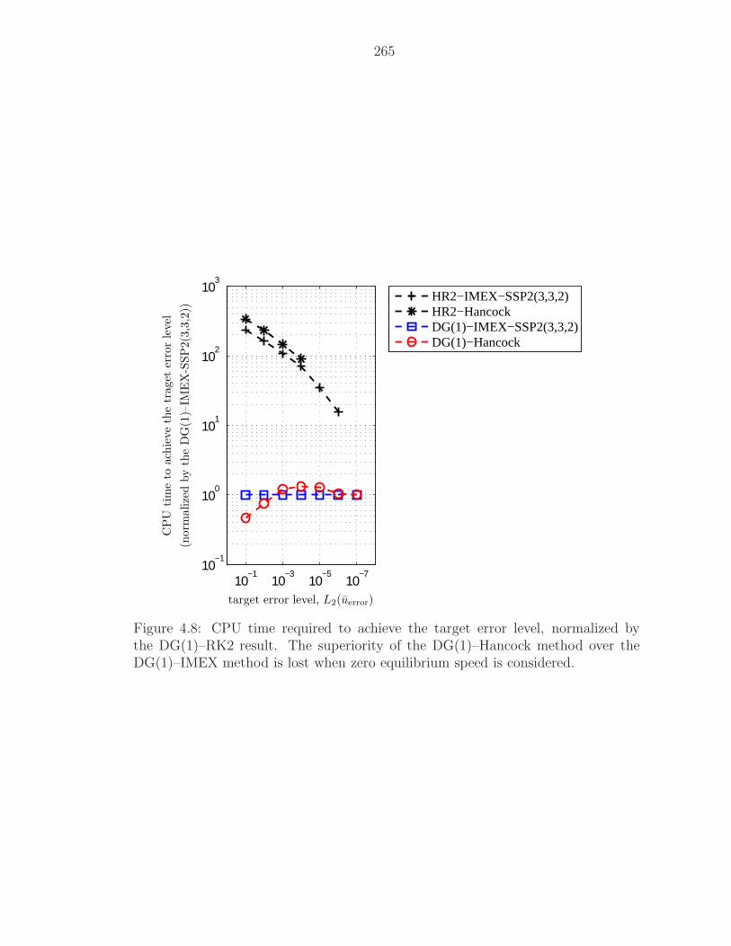
265
10−7
10−5
10−3
10−1
10−1
100
101
102
103
HR2−IMEX−SSP2(3,3,2)HR2−HancockDG(1)−IMEX−SSP2(3,3,2)DG(1)−Hancock
target error level, L2(uerror)
CP
Utim
eto
ach
ieve
the
traget
erro
rle
vel
(norm
alize
dby
the
DG
(1)–
IME
X-S
SP
2(3
,3,2
))
Figure 4.8: CPU time required to achieve the target error level, normalized bythe DG(1)–RK2 result. The superiority of the DG(1)–Hancock method over theDG(1)–IMEX method is lost when zero equilibrium speed is considered.
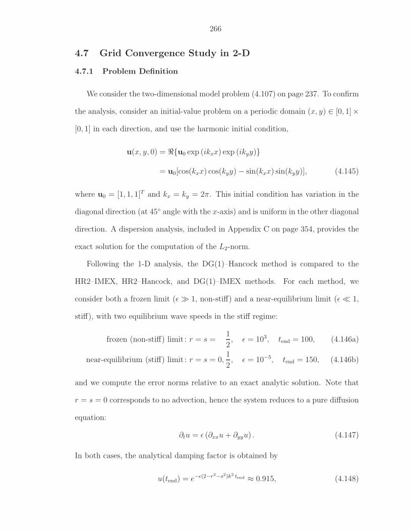
266
4.7 Grid Convergence Study in 2-D
4.7.1 Problem Definition
We consider the two-dimensional model problem (4.107) on page 237. To confirm
the analysis, consider an initial-value problem on a periodic domain (x, y) ∈ [0, 1]×
[0, 1] in each direction, and use the harmonic initial condition,
u(x, y, 0) = ℜu0 exp (ikxx) exp (ikyy)
= u0[cos(kxx) cos(kyy) − sin(kxx) sin(kyy)], (4.145)
where u0 = [1, 1, 1]T and kx = ky = 2π. This initial condition has variation in the
diagonal direction (at 45 angle with the x-axis) and is uniform in the other diagonal
direction. A dispersion analysis, included in Appendix C on page 354, provides the
exact solution for the computation of the L2-norm.
Following the 1-D analysis, the DG(1)–Hancock method is compared to the
HR2–IMEX, HR2–Hancock, and DG(1)–IMEX methods. For each method, we
consider both a frozen limit (ǫ ≫ 1, non-stiff) and a near-equilibrium limit (ǫ ≪ 1,
stiff), with two equilibrium wave speeds in the stiff regime:
frozen (non-stiff) limit : r = s =1
2, ǫ = 103, tend = 100, (4.146a)
near-equilibrium (stiff) limit : r = s = 0,1
2, ǫ = 10−5, tend = 150, (4.146b)
and we compute the error norms relative to an exact analytic solution. Note that
r = s = 0 corresponds to no advection, hence the system reduces to a pure diffusion
equation:
∂tu = ǫ (∂xxu + ∂yyu) . (4.147)
In both cases, the analytical damping factor is obtained by
u(tend) = e−ǫ(2−r2−s2)k2 tend ≈ 0.915, (4.148)
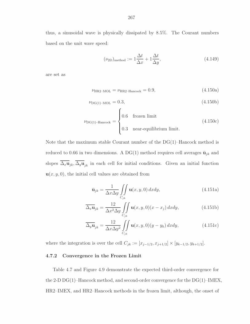
267
thus, a sinusoidal wave is physically dissipated by 8.5%. The Courant numbers
based on the unit wave speed:
(ν2D)method := 1∆t
∆x+ 1
∆t
∆y, (4.149)
are set as
νHR2–MOL = νHR2–Hancock = 0.9, (4.150a)
νDG(1)–MOL = 0.3, (4.150b)
νDG(1)–Hancock =
0.6 frozen limit
0.3 near-equilibrium limit.
(4.150c)
Note that the maximum stable Courant number of the DG(1)–Hancock method is
reduced to 0.66 in two dimensions. A DG(1) method requires cell averages ujk and
slopes ∆xujk, ∆yujk in each cell for initial conditions. Given an initial function
u(x, y, 0), the initial cell values are obtained from
ujk =1
∆x∆y
∫∫
Cjk
u(x, y, 0) dxdy, (4.151a)
∆xujk =12
∆x2∆y
∫∫
Cjk
u(x, y, 0)(x − xj) dxdy, (4.151b)
∆yujk =12
∆x∆y2
∫∫
Cjk
u(x, y, 0)(y − yk) dxdy, (4.151c)
where the integration is over the cell Cjk := [xj−1/2, xj+1/2] × [yk−1/2, yk+1/2].
4.7.2 Convergence in the Frozen Limit
Table 4.7 and Figure 4.9 demonstrate the expected third-order convergence for
the 2-D DG(1)–Hancock method, and second-order convergence for the DG(1)–IMEX,
HR2–IMEX, and HR2–Hancock methods in the frozen limit, although, the onset of
268
the asymptotic convergence rate requires slightly more points per dimension than
in 1D. We note that in this frozen problem the initial-value distribution propagates
along the diagonal of the domain, which produces an effective mesh size in the prop-
agation direction larger than h by a factor√
2. This factor is enough to explain the
difference between the 1-D and 2-D results. Figure 4.10 shows the normalized CPU
time to achieve the target error level. The high efficiency of the DG(1)–Hancock
method is evident.
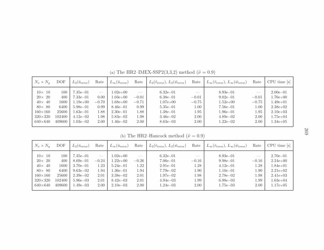
269
(a) The HR2–IMEX-SSP2(3,3,2) method (ν = 0.9)
Nx ×Ny DOF L2(uerror) Rate L∞(uerror) Rate L2(verror), L2(werror) Rate L∞(verror), L∞(werror) Rate CPU time [s]
10× 10 100 7.35e−01 — 1.02e+00 — 6.32e−01 — 8.93e−01 — 2.00e−0120× 20 400 7.33e−01 0.00 1.03e+00 −0.01 6.38e−01 −0.01 9.02e−01 −0.01 1.76e+0040× 40 1600 1.19e+00 −0.70 1.68e+00 −0.71 1.07e+00 −0.75 1.52e+00 −0.75 1.49e+0180× 80 6400 5.98e−01 0.99 8.46e−01 0.99 5.35e−01 1.00 7.56e−01 1.00 2.38e+02
160×160 25600 1.63e−01 1.88 2.30e−01 1.88 1.38e−01 1.95 1.96e−01 1.95 2.10e+03320×320 102400 4.12e−02 1.98 5.83e−02 1.98 3.46e−02 2.00 4.89e−02 2.00 1.75e+04640×640 409600 1.03e−02 2.00 1.46e−02 2.00 8.63e−03 2.00 1.22e−02 2.00 1.34e+05
(b) The HR2–Hancock method (ν = 0.9)
Nx ×Ny DOF L2(uerror) Rate L∞(uerror) Rate L2(verror), L2(werror) Rate L∞(verror), L∞(werror) Rate CPU time [s]
10× 10 100 7.35e−01 — 1.02e+00 — 6.32e−01 — 8.93e−01 — 2.70e−0120× 20 400 8.69e−01 −0.24 1.22e+00 −0.26 7.06e−01 −0.16 9.98e−01 −0.16 2.24e+0040× 40 1600 3.70e−01 1.23 5.24e−01 1.22 2.91e−01 1.28 4.12e−01 1.28 1.84e+0180× 80 6400 9.63e−02 1.94 1.36e−01 1.94 7.79e−02 1.90 1.10e−01 1.90 2.21e+02
160×160 25600 2.39e−02 2.01 3.38e−02 2.01 1.97e−02 1.98 2.78e−02 1.98 2.41e+03320×320 102400 5.96e−03 2.01 8.42e−03 2.01 4.94e−03 1.99 6.98e−03 1.99 1.63e+04640×640 409600 1.49e−03 2.00 2.10e−03 2.00 1.24e−03 2.00 1.75e−03 2.00 1.17e+05
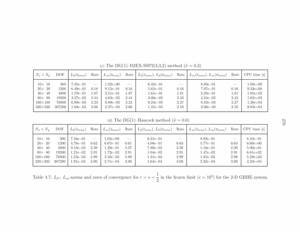
270
(c) The DG(1)–IMEX-SSP2(3,3,2) method (ν = 0.3)
Nx ×Ny DOF L2(uerror) Rate L∞(uerror) Rate L2(verror), L2(werror) Rate L∞(verror), L∞(werror) Rate CPU time [s]
10× 10 300 7.35e−01 — 1.02e+00 — 6.32e−01 — 8.93e−01 — 1.08e+0020× 20 1200 6.49e−01 0.18 9.15e−01 0.16 5.65e−01 0.16 7.97e−01 0.16 9.33e+0040× 40 4800 1.78e−01 1.87 2.51e−01 1.87 1.61e−01 1.81 2.28e−01 1.81 1.05e+0280× 80 19200 3.27e−02 2.44 4.63e−02 2.44 3.00e−02 2.43 4.24e−02 2.42 1.62e+03
160×160 76800 6.99e−03 2.23 9.89e−03 2.23 6.24e−03 2.27 8.82e−03 2.27 1.26e+04320×320 307200 1.68e−03 2.06 2.37e−03 2.06 1.45e−03 2.10 2.06e−03 2.10 9.83e+04
(d) The DG(1)–Hancock method (ν = 0.6)
Nx ×Ny DOF L2(uerror) Rate L∞(uerror) Rate L2(verror), L2(werror) Rate L∞(verror), L∞(werror) Rate CPU time [s]
10× 10 300 7.34e−01 — 1.02e+00 — 6.31e−01 — 8.92e−01 — 8.10e−0120× 20 1200 4.78e−01 0.62 6.67e−01 0.61 4.08e−01 0.63 5.77e−01 0.63 6.60e+0040× 40 4800 9.13e−02 2.39 1.29e−01 2.37 7.80e−02 2.39 1.10e−01 2.39 5.90e+0180× 80 19200 1.21e−02 2.91 1.72e−02 2.91 1.04e−02 2.91 1.47e−02 2.91 6.61e+02
160×160 76800 1.53e−03 2.99 2.16e−03 2.99 1.31e−03 2.99 1.85e−03 2.99 5.29e+03320×320 307200 1.91e−04 3.00 2.71e−04 3.00 1.64e−04 3.00 2.32e−04 3.00 4.23e+04
Table 4.7: L2-, L∞-norms and rates of convergence for r = s =1
2in the frozen limit (ǫ = 103) for the 2-D GHHE system.
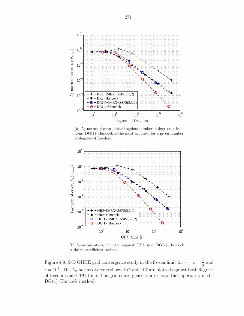
271
102
103
104
105
106
10−4
10−3
10−2
10−1
100
101
HR2−IMEX−SSP2(3,3,2)HR2−HancockDG(1)−IMEX−SSP2(3,3,2)DG(1)−Hancock
degrees of freedom
L2-n
orm
ofer
ror,L
2(u
err
or)
(a) L2-norms of error plotted against number of degrees of free-dom. DG(1)–Hancock is the most accurate for a given numberof degrees of freedom.
100
102
104
106
10−4
10−3
10−2
10−1
100
101
HR2−IMEX−SSP2(3,3,2)HR2−HancockDG(1)−IMEX−SSP2(3,3,2)DG(1)−Hancock
CPU time [s]
L2-n
orm
ofer
ror,L
2(u
err
or)
(b) L2-norms of error plotted against CPU time. DG(1)–Hancockis the most efficient method.
Figure 4.9: 2-D GHHE grid convergence study in the frozen limit for r = s =1
2and
ǫ = 103. The L2-norms of errors shown in Table 4.7 are plotted against both degreesof freedom and CPU time. The grid-convergence study shows the superiority of theDG(1)–Hancock method.
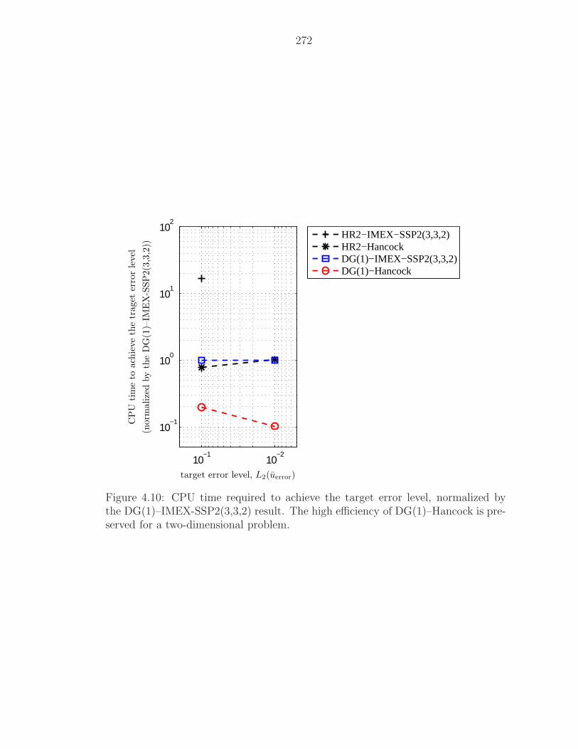
272
10−2
10−1
10−1
100
101
102
HR2−IMEX−SSP2(3,3,2)HR2−HancockDG(1)−IMEX−SSP2(3,3,2)DG(1)−Hancock
target error level, L2(uerror)
CP
Utim
eto
ach
ieve
the
traget
erro
rle
vel
(norm
alize
dby
the
DG
(1)–
IME
X-S
SP
2(3
,3,2
))
Figure 4.10: CPU time required to achieve the target error level, normalized bythe DG(1)–IMEX-SSP2(3,3,2) result. The high efficiency of DG(1)–Hancock is pre-served for a two-dimensional problem.
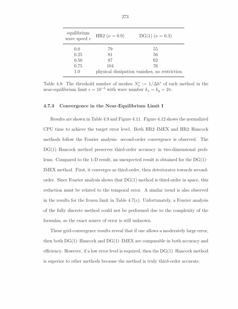
273
equilibriumHR2 (ν = 0.9) DG(1) (ν = 0.3)
wave speed r
0.0 79 550.25 81 560.50 87 620.75 104 761.0 physical dissipation vanishes, no restriction
Table 4.8: The threshold number of meshes N∗x := 1/∆h∗ of each method in the
near-equilibrium limit ǫ = 10−5 with wave number kx = ky = 2π.
4.7.3 Convergence in the Near-Equilibrium Limit I
Results are shown in Table 4.9 and Figure 4.11. Figure 4.12 shows the normalized
CPU time to achieve the target error level. Both HR2–IMEX and HR2–Hancock
methods follow the Fourier analysis: second-order convergence is observed. The
DG(1)–Hancock method preserves third-order accuracy in two-dimensional prob-
lems. Compared to the 1-D result, an unexpected result is obtained for the DG(1)–
IMEX method. First, it converges as third-order, then deteriorates towards second-
order. Since Fourier analysis shows that DG(1) method is third-order in space, this
reduction must be related to the temporal error. A similar trend is also observed
in the results for the frozen limit in Table 4.7(c). Unfortunately, a Fourier analysis
of the fully discrete method could not be performed due to the complexity of the
formulas, so the exact source of error is still unknown.
These grid-convergence results reveal that if one allows a moderately large error,
then both DG(1)–Hancock and DG(1)–IMEX are comparable in both accuracy and
efficiency. However, if a low error level is required, then the DG(1)–Hancock method
is superior to other methods because the method is truly third-order accurate.
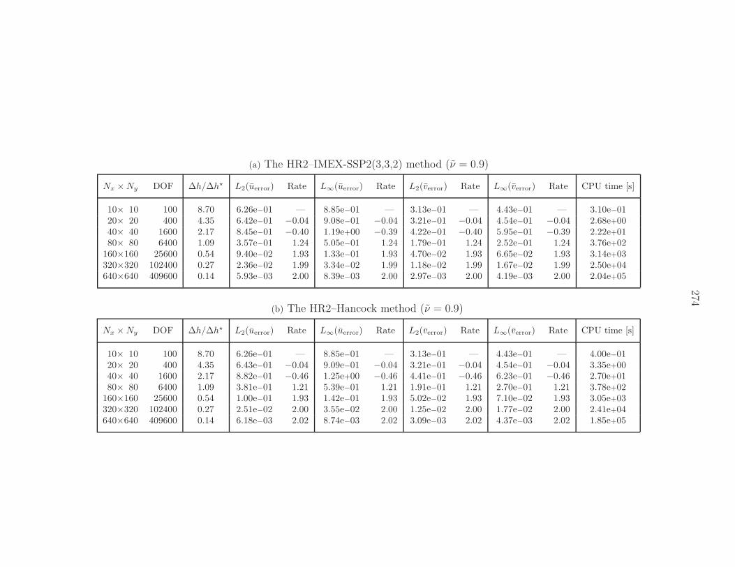
274
(a) The HR2–IMEX-SSP2(3,3,2) method (ν = 0.9)
Nx ×Ny DOF ∆h/∆h⋆ L2(uerror) Rate L∞(uerror) Rate L2(verror) Rate L∞(verror) Rate CPU time [s]
10× 10 100 8.70 6.26e−01 — 8.85e−01 — 3.13e−01 — 4.43e−01 — 3.10e−0120× 20 400 4.35 6.42e−01 −0.04 9.08e−01 −0.04 3.21e−01 −0.04 4.54e−01 −0.04 2.68e+0040× 40 1600 2.17 8.45e−01 −0.40 1.19e+00 −0.39 4.22e−01 −0.40 5.95e−01 −0.39 2.22e+0180× 80 6400 1.09 3.57e−01 1.24 5.05e−01 1.24 1.79e−01 1.24 2.52e−01 1.24 3.76e+02
160×160 25600 0.54 9.40e−02 1.93 1.33e−01 1.93 4.70e−02 1.93 6.65e−02 1.93 3.14e+03320×320 102400 0.27 2.36e−02 1.99 3.34e−02 1.99 1.18e−02 1.99 1.67e−02 1.99 2.50e+04640×640 409600 0.14 5.93e−03 2.00 8.39e−03 2.00 2.97e−03 2.00 4.19e−03 2.00 2.04e+05
(b) The HR2–Hancock method (ν = 0.9)
Nx ×Ny DOF ∆h/∆h⋆ L2(uerror) Rate L∞(uerror) Rate L2(verror) Rate L∞(verror) Rate CPU time [s]
10× 10 100 8.70 6.26e−01 — 8.85e−01 — 3.13e−01 — 4.43e−01 — 4.00e−0120× 20 400 4.35 6.43e−01 −0.04 9.09e−01 −0.04 3.21e−01 −0.04 4.54e−01 −0.04 3.35e+0040× 40 1600 2.17 8.82e−01 −0.46 1.25e+00 −0.46 4.41e−01 −0.46 6.23e−01 −0.46 2.70e+0180× 80 6400 1.09 3.81e−01 1.21 5.39e−01 1.21 1.91e−01 1.21 2.70e−01 1.21 3.78e+02
160×160 25600 0.54 1.00e−01 1.93 1.42e−01 1.93 5.02e−02 1.93 7.10e−02 1.93 3.05e+03320×320 102400 0.27 2.51e−02 2.00 3.55e−02 2.00 1.25e−02 2.00 1.77e−02 2.00 2.41e+04640×640 409600 0.14 6.18e−03 2.02 8.74e−03 2.02 3.09e−03 2.02 4.37e−03 2.02 1.85e+05
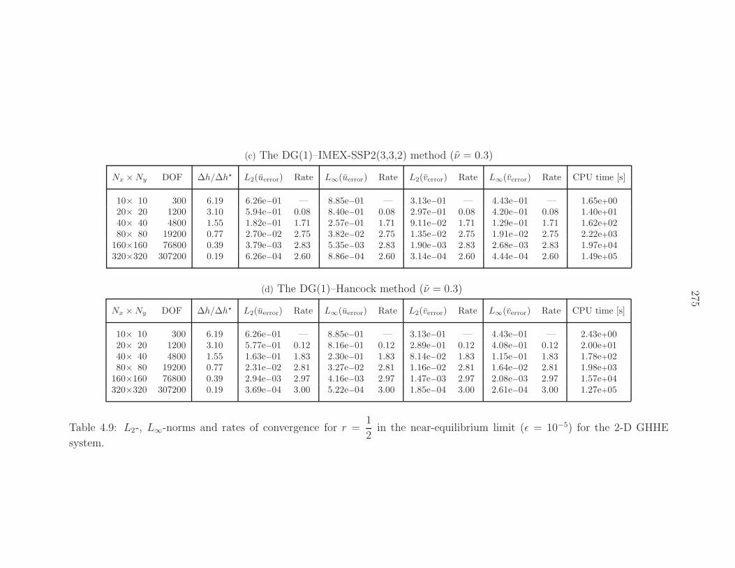
275
(c) The DG(1)–IMEX-SSP2(3,3,2) method (ν = 0.3)
Nx ×Ny DOF ∆h/∆h⋆ L2(uerror) Rate L∞(uerror) Rate L2(verror) Rate L∞(verror) Rate CPU time [s]
10× 10 300 6.19 6.26e−01 — 8.85e−01 — 3.13e−01 — 4.43e−01 — 1.65e+0020× 20 1200 3.10 5.94e−01 0.08 8.40e−01 0.08 2.97e−01 0.08 4.20e−01 0.08 1.40e+0140× 40 4800 1.55 1.82e−01 1.71 2.57e−01 1.71 9.11e−02 1.71 1.29e−01 1.71 1.62e+0280× 80 19200 0.77 2.70e−02 2.75 3.82e−02 2.75 1.35e−02 2.75 1.91e−02 2.75 2.22e+03
160×160 76800 0.39 3.79e−03 2.83 5.35e−03 2.83 1.90e−03 2.83 2.68e−03 2.83 1.97e+04320×320 307200 0.19 6.26e−04 2.60 8.86e−04 2.60 3.14e−04 2.60 4.44e−04 2.60 1.49e+05
(d) The DG(1)–Hancock method (ν = 0.3)
Nx ×Ny DOF ∆h/∆h⋆ L2(uerror) Rate L∞(uerror) Rate L2(verror) Rate L∞(verror) Rate CPU time [s]
10× 10 300 6.19 6.26e−01 — 8.85e−01 — 3.13e−01 — 4.43e−01 — 2.43e+0020× 20 1200 3.10 5.77e−01 0.12 8.16e−01 0.12 2.89e−01 0.12 4.08e−01 0.12 2.00e+0140× 40 4800 1.55 1.63e−01 1.83 2.30e−01 1.83 8.14e−02 1.83 1.15e−01 1.83 1.78e+0280× 80 19200 0.77 2.31e−02 2.81 3.27e−02 2.81 1.16e−02 2.81 1.64e−02 2.81 1.98e+03
160×160 76800 0.39 2.94e−03 2.97 4.16e−03 2.97 1.47e−03 2.97 2.08e−03 2.97 1.57e+04320×320 307200 0.19 3.69e−04 3.00 5.22e−04 3.00 1.85e−04 3.00 2.61e−04 3.00 1.27e+05
Table 4.9: L2-, L∞-norms and rates of convergence for r =1
2in the near-equilibrium limit (ǫ = 10−5) for the 2-D GHHE
system.
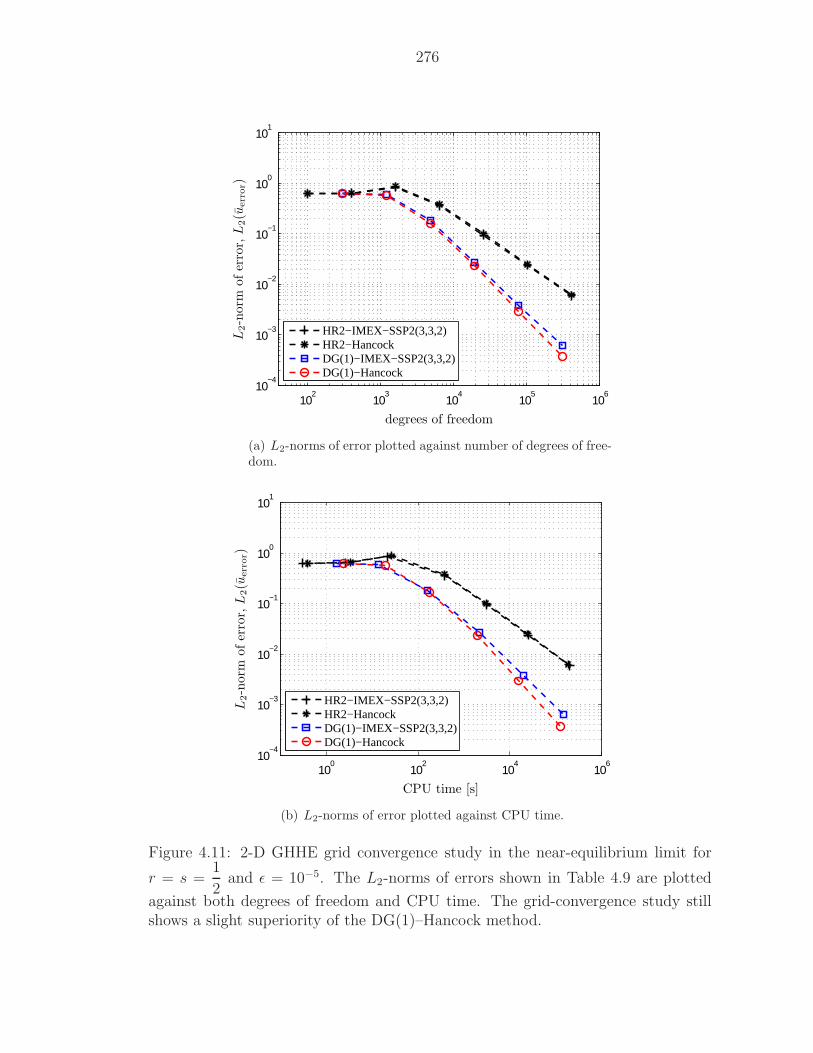
276
102
103
104
105
106
10−4
10−3
10−2
10−1
100
101
HR2−IMEX−SSP2(3,3,2)HR2−HancockDG(1)−IMEX−SSP2(3,3,2)DG(1)−Hancock
degrees of freedom
L2-n
orm
ofer
ror,L
2(u
err
or)
(a) L2-norms of error plotted against number of degrees of free-dom.
100
102
104
106
10−4
10−3
10−2
10−1
100
101
HR2−IMEX−SSP2(3,3,2)HR2−HancockDG(1)−IMEX−SSP2(3,3,2)DG(1)−Hancock
CPU time [s]
L2-n
orm
ofer
ror,L
2(u
err
or)
(b) L2-norms of error plotted against CPU time.
Figure 4.11: 2-D GHHE grid convergence study in the near-equilibrium limit for
r = s =1
2and ǫ = 10−5. The L2-norms of errors shown in Table 4.9 are plotted
against both degrees of freedom and CPU time. The grid-convergence study stillshows a slight superiority of the DG(1)–Hancock method.
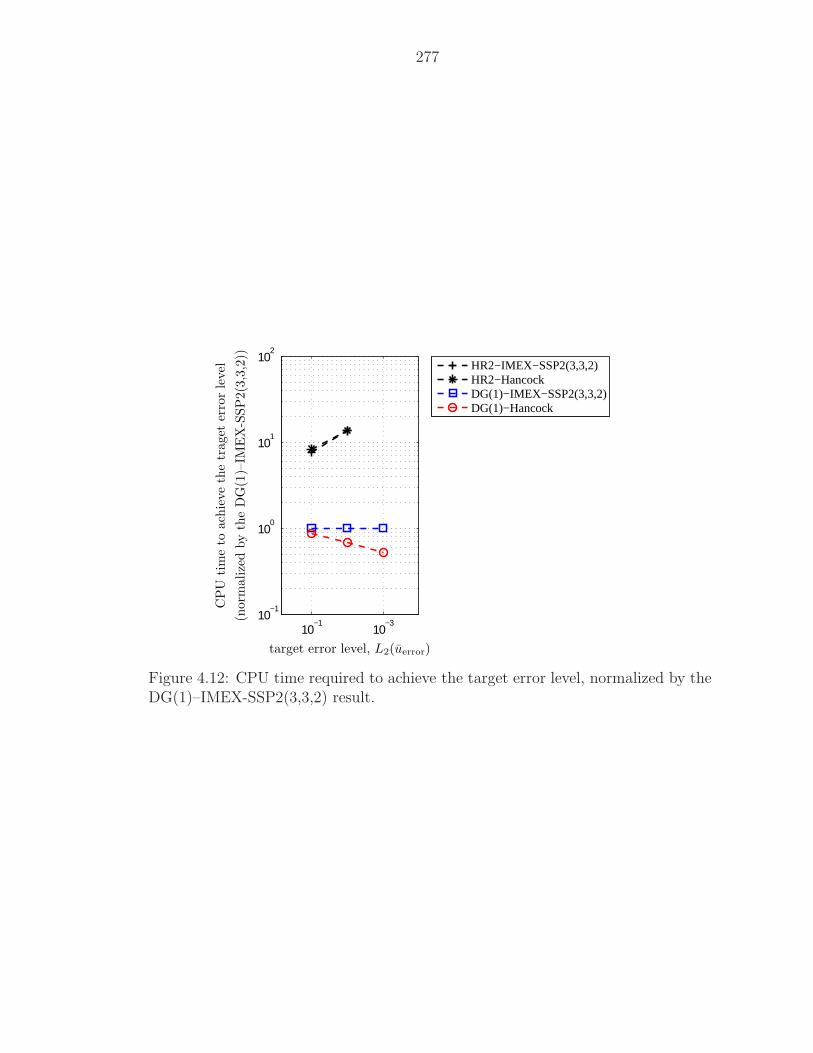
277
10−3
10−1
10−1
100
101
102
HR2−IMEX−SSP2(3,3,2)HR2−HancockDG(1)−IMEX−SSP2(3,3,2)DG(1)−Hancock
target error level, L2(uerror)
CP
Utim
eto
ach
ieve
the
traget
erro
rle
vel
(norm
alize
dby
the
DG
(1)–
IME
X-S
SP
2(3
,3,2
))
Figure 4.12: CPU time required to achieve the target error level, normalized by theDG(1)–IMEX-SSP2(3,3,2) result.
278
4.7.4 Convergence in the Near-Equilibrium Limit II
In a single dimension, both DG(1)–IMEX and DG(1)–Hancock methods for
r = 0 do not appear to have a threshold above which numerical dissipation domi-
nates over physical dissipation. However, problems of practical significance are mul-
tidimensional, and multiple dimensions frequently introduce additional couplings.
Analysis suggests that part of the multidimensional error is independent of the wave
speeds, and causes the mesh-size restriction even when zero wave speeds, r = s = 0,
are considered. To gauge whether 2-D DG(1) methods actually exhibit this behav-
ior, we conduct a two-dimensional numerical experiment.
The results are shown in Table 4.10 and Figure 4.13. Figure 4.14 shows the
normalized CPU time to achieve the target error level. It is observed that all four
methods converge with third-order accuracy. This can be understood again by the
Fourier analysis given in (4.136) on page 245. Even though the analyses do not
include the temporal discretization error, they predict third-order convergence on
coarse grids for both HR2 and DG(1) spatial discretizations. When the grids become
finer, we expect a reduction to second-order convergence because the spatial error
is proportional to ǫ∆h2. The dominant dissipation error of the DG(1) method is
1
3of that of HR2, but Figure 4.13 appears to indicate the opposite; the reason is
that DG(1) uses three times as more degrees of freedom as HR2. In the end, the
errors of both methods are quite comparable. These numerical results show that
the DG(1) spatial discretization loses its superiority to HR2 in the near-equilibrium
limit with r = s = 0.
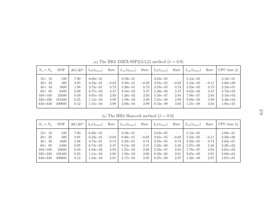
279
(a) The HR2–IMEX-SSP2(3,3,2) method (ν = 0.9)
Nx ×Ny DOF ∆h/∆h⋆ L2(uerror) Rate L∞(uerror) Rate L2(verror) Rate L∞(verror) Rate CPU time [s]
10× 10 100 7.90 6.08e−01 — 8.59e−01 — 3.82e−05 — 5.14e−05 — 3.10e−0120× 20 400 3.95 6.23e−01 −0.03 8.80e−01 −0.03 3.91e−05 −0.03 5.53e−05 −0.11 2.66e+0040× 40 1600 1.98 3.75e−01 0.73 5.30e−01 0.73 2.35e−05 0.73 3.33e−05 0.73 2.23e+0180× 80 6400 0.99 6.77e−02 2.47 9.58e−02 2.47 4.26e−06 2.47 6.02e−06 2.47 3.73e+02
160×160 25600 0.49 8.91e−03 2.93 1.26e−02 2.93 5.56e−07 2.94 7.86e−07 2.94 3.16e+03320×320 102400 0.25 1.12e−03 2.99 1.59e−03 2.99 7.01e−08 2.99 9.92e−08 2.99 2.46e+04640×640 409600 0.12 1.41e−04 2.99 2.00e−04 2.99 8.54e−09 3.04 1.21e−08 3.04 1.95e+05
(b) The HR2–Hancock method (ν = 0.9)
Nx ×Ny DOF ∆h/∆h⋆ L2(uerror) Rate L∞(uerror) Rate L2(verror) Rate L∞(verror) Rate CPU time [s]
10× 10 100 7.90 6.08e−01 — 8.59e−01 — 3.82e−05 — 5.14e−05 — 4.00e−0120× 20 400 3.95 6.23e−01 −0.03 8.80e−01 −0.03 3.91e−05 −0.03 5.53e−05 −0.11 3.30e+0040× 40 1600 1.98 3.74e−01 0.74 5.29e−01 0.74 2.35e−05 0.74 3.32e−05 0.74 2.63e+0180× 80 6400 0.99 6.74e−02 2.47 9.54e−02 2.47 4.22e−06 2.48 5.97e−06 2.48 3.28e+02
160×160 25600 0.49 8.83e−03 2.93 1.25e−02 2.93 5.50e−07 2.94 7.78e−07 2.94 2.65e+03320×320 102400 0.25 1.11e−03 3.00 1.56e−03 3.00 6.82e−08 3.01 9.65e−08 3.01 2.08e+04640×640 409600 0.12 1.53e−04 2.85 2.17e−04 2.85 9.37e−09 2.87 1.32e−08 2.87 1.67e+05
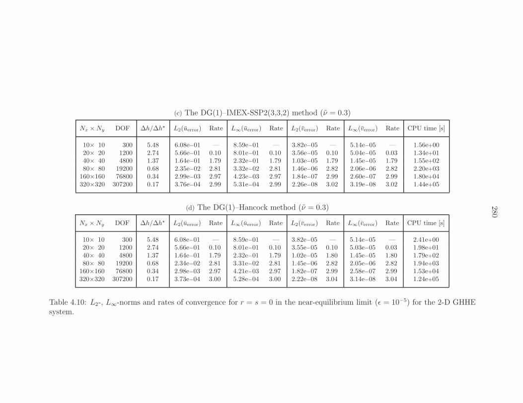
280
(c) The DG(1)–IMEX-SSP2(3,3,2) method (ν = 0.3)
Nx ×Ny DOF ∆h/∆h⋆ L2(uerror) Rate L∞(uerror) Rate L2(verror) Rate L∞(verror) Rate CPU time [s]
10× 10 300 5.48 6.08e−01 — 8.59e−01 — 3.82e−05 — 5.14e−05 — 1.56e+0020× 20 1200 2.74 5.66e−01 0.10 8.01e−01 0.10 3.56e−05 0.10 5.04e−05 0.03 1.34e+0140× 40 4800 1.37 1.64e−01 1.79 2.32e−01 1.79 1.03e−05 1.79 1.45e−05 1.79 1.55e+0280× 80 19200 0.68 2.35e−02 2.81 3.32e−02 2.81 1.46e−06 2.82 2.06e−06 2.82 2.20e+03
160×160 76800 0.34 2.99e−03 2.97 4.23e−03 2.97 1.84e−07 2.99 2.60e−07 2.99 1.80e+04320×320 307200 0.17 3.76e−04 2.99 5.31e−04 2.99 2.26e−08 3.02 3.19e−08 3.02 1.44e+05
(d) The DG(1)–Hancock method (ν = 0.3)
Nx ×Ny DOF ∆h/∆h⋆ L2(uerror) Rate L∞(uerror) Rate L2(verror) Rate L∞(verror) Rate CPU time [s]
10× 10 300 5.48 6.08e−01 — 8.59e−01 — 3.82e−05 — 5.14e−05 — 2.41e+0020× 20 1200 2.74 5.66e−01 0.10 8.01e−01 0.10 3.55e−05 0.10 5.03e−05 0.03 1.98e+0140× 40 4800 1.37 1.64e−01 1.79 2.32e−01 1.79 1.02e−05 1.80 1.45e−05 1.80 1.79e+0280× 80 19200 0.68 2.34e−02 2.81 3.31e−02 2.81 1.45e−06 2.82 2.05e−06 2.82 1.94e+03
160×160 76800 0.34 2.98e−03 2.97 4.21e−03 2.97 1.82e−07 2.99 2.58e−07 2.99 1.53e+04320×320 307200 0.17 3.73e−04 3.00 5.28e−04 3.00 2.22e−08 3.04 3.14e−08 3.04 1.24e+05
Table 4.10: L2-, L∞-norms and rates of convergence for r = s = 0 in the near-equilibrium limit (ǫ = 10−5) for the 2-D GHHEsystem.
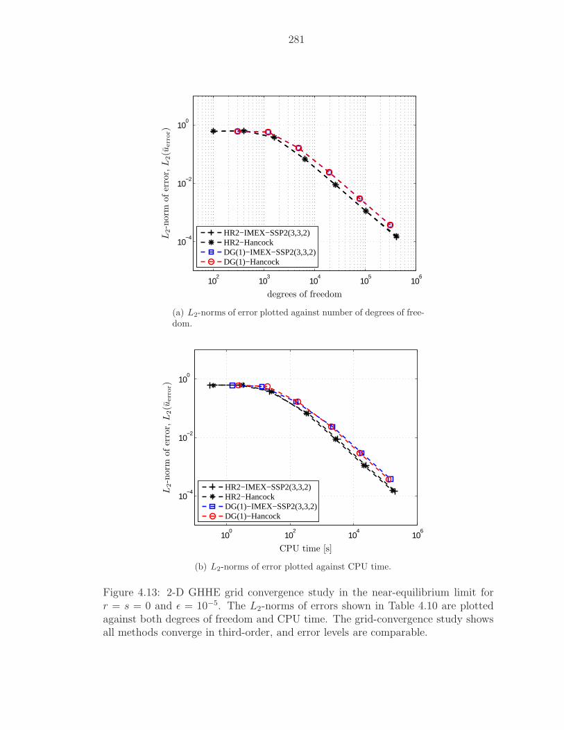
281
102
103
104
105
106
10−4
10−2
100
HR2−IMEX−SSP2(3,3,2)HR2−HancockDG(1)−IMEX−SSP2(3,3,2)DG(1)−Hancock
degrees of freedom
L2-n
orm
ofer
ror,L
2(u
err
or)
(a) L2-norms of error plotted against number of degrees of free-dom.
100
102
104
106
10−4
10−2
100
HR2−IMEX−SSP2(3,3,2)HR2−HancockDG(1)−IMEX−SSP2(3,3,2)DG(1)−Hancock
CPU time [s]
L2-n
orm
ofer
ror,L
2(u
err
or)
(b) L2-norms of error plotted against CPU time.
Figure 4.13: 2-D GHHE grid convergence study in the near-equilibrium limit forr = s = 0 and ǫ = 10−5. The L2-norms of errors shown in Table 4.10 are plottedagainst both degrees of freedom and CPU time. The grid-convergence study showsall methods converge in third-order, and error levels are comparable.
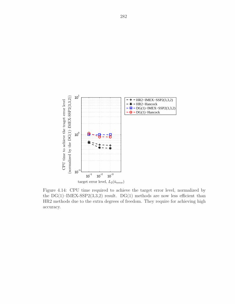
282
10−3
10−2
10−1
10−1
100
101
HR2−IMEX−SSP2(3,3,2)HR2−HancockDG(1)−IMEX−SSP2(3,3,2)DG(1)−Hancock
target error level, L2(uerror)
CP
Utim
eto
ach
ieve
the
traget
erro
rle
vel
(norm
alize
dby
the
DG
(1)–
IME
X-S
SP
2(3
,3,2
))
Figure 4.14: CPU time required to achieve the target error level, normalized bythe DG(1)–IMEX-SSP2(3,3,2) result. DG(1) methods are now less efficient thanHR2 methods due to the extra degrees of freedom. They require for achieving highaccuracy.
283
4.8 Grid-Convergence Study for Nonlinear Hyperbolic–Relaxation Equations
4.8.1 The Euler Equations with Heat Transfer
To demonstrate the accuracy of the DG(1)–Hancock method when applied to
a nonlinear hyperbolic-relaxation system, the Euler equations with heat transfer,
which reduce to the isothermal Euler equations in the equilibrium limit, are adopted
as a model equation [Pem93b]:
∂
∂t
ρ
ρu
ρE
+∂
∂x
ρu
ρu2 + p
ρuH
= −1
ǫ
0
0
ρ(T − T0)
, (4.152)
where the pressure is given by the ideal gas law, p := (γ − 1)ρe = ρRT . The frozen
characteristic speeds are u±a, u, where the speed of sound is given by a :=√
γp/ρ.
In the equilibrium limit (ǫ → 0), the nonequilibrium temperature T converges to
the constant equilibrium temperature T0 instantaneously. As a result, the above
equations tend asymptotically to the following isothermal Euler equations:
∂
∂t
ρ
ρu
+
∂
∂x
ρu
ρu2 + p∗
=
0
0
, (4.153)
where the gas becomes polytropic with equilibrium γ = 1 and the pressure is given
by p∗(ρ) := ρRT0. The equilibrium characteristic speeds are u ± a∗, where the
constant speed of sound is a∗ :=√
p∗/ρ =√
RT0.
284
Consider an initial-value problem with the following C∞ initial distributions:
ρ0(x) = exp
(u0(x)
a∗
), (4.154a)
u0(x) =
−a∗, x < −5,
a∗ tanh
[− 10x
(x + 5)(x − 5)
], x ∈ [−5, 5],
a∗, x > 5,
(4.154b)
p0(x) = (a∗)2ρ0(x), (4.154c)
plotted in Figure 4.15. The initial conditions are chosen such that the analytical
solution of the isothermal Euler equations becomes a simple wave solution; one of
the Riemann invariants remains constant: J−iso(x, t) = ln ρ0 −
u0
a∗≡ 0. Also, the flow
properties are non-equilibrium (T 6= T0) only within the domain x ∈ [−5, 5]. The
equilibrium speed of sound, equilibrium temperature, and the ratio of specific heats
are taken to be:
a∗ =√
0.4, T0 = 1, γ = 1.4. (4.155)
The computational domain is confined to x ∈ [−16, 16] with uniform meshes, and
the solution at the time tend = 5.0 is used for checking grid convergence and com-
parison among methods.
Richardson Extrapolation for Grid Convergence
In order to determine the order of accuracy of the various schemes, we need to
know the exact solution of (4.152) at the time tend. When the frozen limit (ǫ → ∞)
is considered, the exact solution can be obtained with the regular Euler equations.
Conversely, at the equilibrium limit (ǫ → 0), the exact solution is derived from the
isothermal Euler equations, (4.153). Simple-wave solutions are available for these
two conservation laws; however, the resulting exact solutions are not strictly the
285
exact solution of (4.152). For instance, when O(ǫ) ≪ 1, an asymptotic expansion
shows that a series of O(ǫk)-term appears on the right-hand side of the conservation
laws,
∂tU + ∂xF(U) = O(ǫ) ∂xxU + . . . . (4.156)
Thus, the actual exact solution should be derived from (4.156), which contains an
infinite series in terms of ǫ. This could be possible if a simple system is considered;
however, the derivation can be cumbersome.
To overcome this difficulty, Richardson extrapolation, which does not require
knowledge of the exact solution, is adopted for the grid-convergence study. In
brief, successive grid solutions provide an estimated exact solution, ui,exact, and the
coefficients of the local truncation error, cj, in the following form:
ui = ui,exact + c1∆x + c2∆x2 + c3∆x3 + . . . . (4.157)
Thus, once the right-hand side of the above equation is computed, the error at the
cell i is given by
errori(u) := ui − ui,exact
= (c1)i∆x + (c2)i∆x2 + (c3)i∆x3 + . . . , (4.158)
after which, the Lp-norm on the uniform grid is obtained by
Lp(u) :=
[1
N
N∑
i=1
|errori(u)|p]1/p
. (4.159)
Numerical Results
The DG(1)–Hancock method is compared to two semi-discrete methods: HR2–MOL
and DG(1)–MOL. As to the time integrator, we adopt the IMEX–SSP2(3,3,2) (2.101).
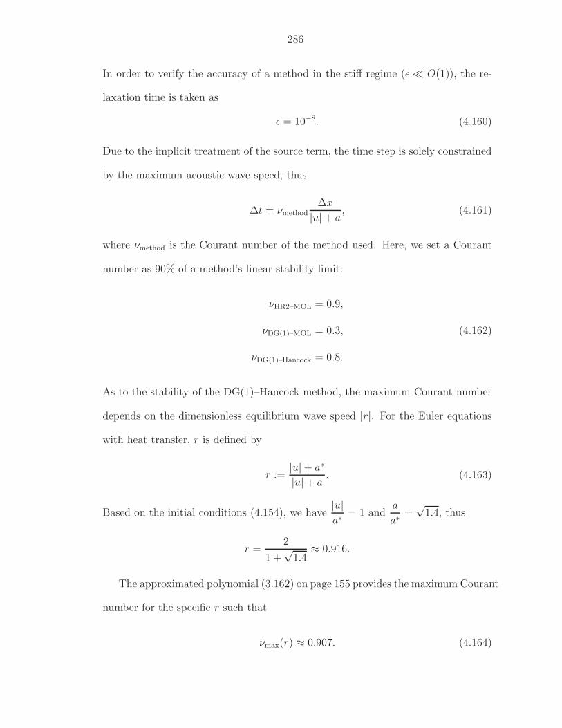
286
In order to verify the accuracy of a method in the stiff regime (ǫ ≪ O(1)), the re-
laxation time is taken as
ǫ = 10−8. (4.160)
Due to the implicit treatment of the source term, the time step is solely constrained
by the maximum acoustic wave speed, thus
∆t = νmethod∆x
|u| + a, (4.161)
where νmethod is the Courant number of the method used. Here, we set a Courant
number as 90% of a method’s linear stability limit:
νHR2–MOL = 0.9,
νDG(1)–MOL = 0.3, (4.162)
νDG(1)–Hancock = 0.8.
As to the stability of the DG(1)–Hancock method, the maximum Courant number
depends on the dimensionless equilibrium wave speed |r|. For the Euler equations
with heat transfer, r is defined by
r :=|u| + a∗
|u| + a. (4.163)
Based on the initial conditions (4.154), we have|u|a∗
= 1 anda
a∗=
√1.4, thus
r =2
1 +√
1.4≈ 0.916.
The approximated polynomial (3.162) on page 155 provides the maximum Courant
number for the specific r such that
νmax(r) ≈ 0.907. (4.164)
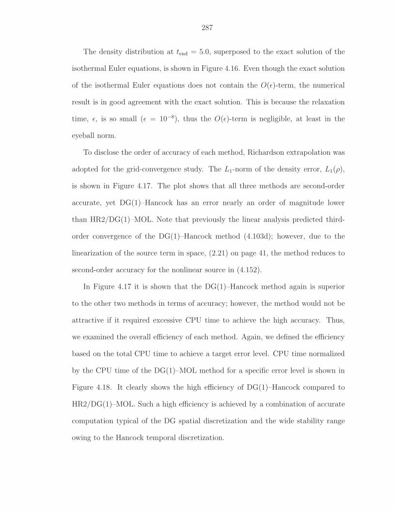
287
The density distribution at tend = 5.0, superposed to the exact solution of the
isothermal Euler equations, is shown in Figure 4.16. Even though the exact solution
of the isothermal Euler equations does not contain the O(ǫ)-term, the numerical
result is in good agreement with the exact solution. This is because the relaxation
time, ǫ, is so small (ǫ = 10−8), thus the O(ǫ)-term is negligible, at least in the
eyeball norm.
To disclose the order of accuracy of each method, Richardson extrapolation was
adopted for the grid-convergence study. The L1-norm of the density error, L1(ρ),
is shown in Figure 4.17. The plot shows that all three methods are second-order
accurate, yet DG(1)–Hancock has an error nearly an order of magnitude lower
than HR2/DG(1)–MOL. Note that previously the linear analysis predicted third-
order convergence of the DG(1)–Hancock method (4.103d); however, due to the
linearization of the source term in space, (2.21) on page 41, the method reduces to
second-order accuracy for the nonlinear source in (4.152).
In Figure 4.17 it is shown that the DG(1)–Hancock method again is superior
to the other two methods in terms of accuracy; however, the method would not be
attractive if it required excessive CPU time to achieve the high accuracy. Thus,
we examined the overall efficiency of each method. Again, we defined the efficiency
based on the total CPU time to achieve a target error level. CPU time normalized
by the CPU time of the DG(1)–MOL method for a specific error level is shown in
Figure 4.18. It clearly shows the high efficiency of DG(1)–Hancock compared to
HR2/DG(1)–MOL. Such a high efficiency is achieved by a combination of accurate
computation typical of the DG spatial discretization and the wide stability range
owing to the Hancock temporal discretization.
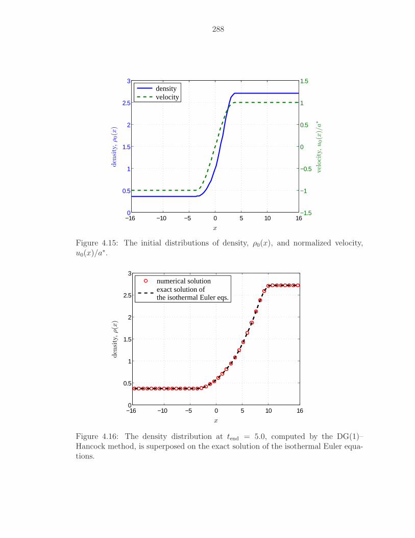
288
−16 −10 −5 0 5 10 160
0.5
1
1.5
2
2.5
3
−1.5
−1
−0.5
0
0.5
1
1.5 density velocity
x
den
sity
,ρ0(x
)
vel
oci
ty,u
0(x
)/a∗
Figure 4.15: The initial distributions of density, ρ0(x), and normalized velocity,u0(x)/a∗.
−16 −10 −5 0 5 10 160
0.5
1
1.5
2
2.5
3
numerical solution exact solution of the isothermal Euler eqs.
x
den
sity
,ρ(x
)
Figure 4.16: The density distribution at tend = 5.0, computed by the DG(1)–Hancock method, is superposed on the exact solution of the isothermal Euler equa-tions.
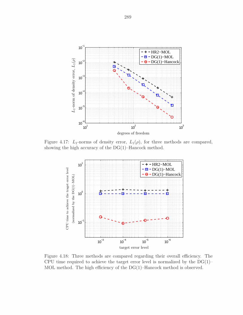
289
101
102
103
10−6
10−5
10−4
10−3
10−2
10−1
HR2−MOLDG(1)−MOLDG(1)−Hancock
degrees of freedom
L1-n
orm
ofden
sity
erro
r,L
1(ρ
)
Figure 4.17: L1-norms of density error, L1(ρ), for three methods are compared,showing the high accuracy of the DG(1)–Hancock method.
10−6
10−5
10−4
10−3
10−1
100
101
HR2−MOLDG(1)−MOLDG(1)−Hancock
target error level
CP
Utim
eto
ach
ieve
the
traget
erro
rle
vel
(norm
alize
dby
the
DG
(1)–
MO
L)
Figure 4.18: Three methods are compared regarding their overall efficiency. TheCPU time required to achieve the target error level is normalized by the DG(1)–MOL method. The high efficiency of the DG(1)–Hancock method is observed.
CHAPTER V
APPLICATION TO EXTENDED
HYDRODYNAMICS (10-MOMENT MODEL)
5.1 Introduction
In this chapter, the DG(1) and HR2 spatial discretization methods are applied
to nonlinear hyperbolic-relaxation equations which describe the motion of fluid,
namely, the 10-moment equations. The 10-moment equations are the best known
and most studied among models that use multiple moments of the Boltzmann equa-
tion [Bro96, Hit00]. Recall the hierarchical relation of the moment approach among
other mathematical models (see Figure 1.2 on page 11).
The 10-moment equations can be derived in several ways. Note that differ-
ent distribution functions could lead to identical macroscopic transport equations.
Gombosi describes the 10-moment equations by simplifying a larger set of moment
equations: the 20-moment equations derived by Grad’s method of moments [Gom94,
pp. 223–224]. He also shows that both 20-moment equations and the model obtained
by the Chapman–Enskog expansion are identical up to the third order in terms of the
relaxation time. Another approach is that of Holway, who replaces the Maxwellian
by an ellipsoidal distribution function [Hol65]. More recently, Levermore derived
the 10-moment model as a member of a hierarchy of moment closures [Lev96]. He
290
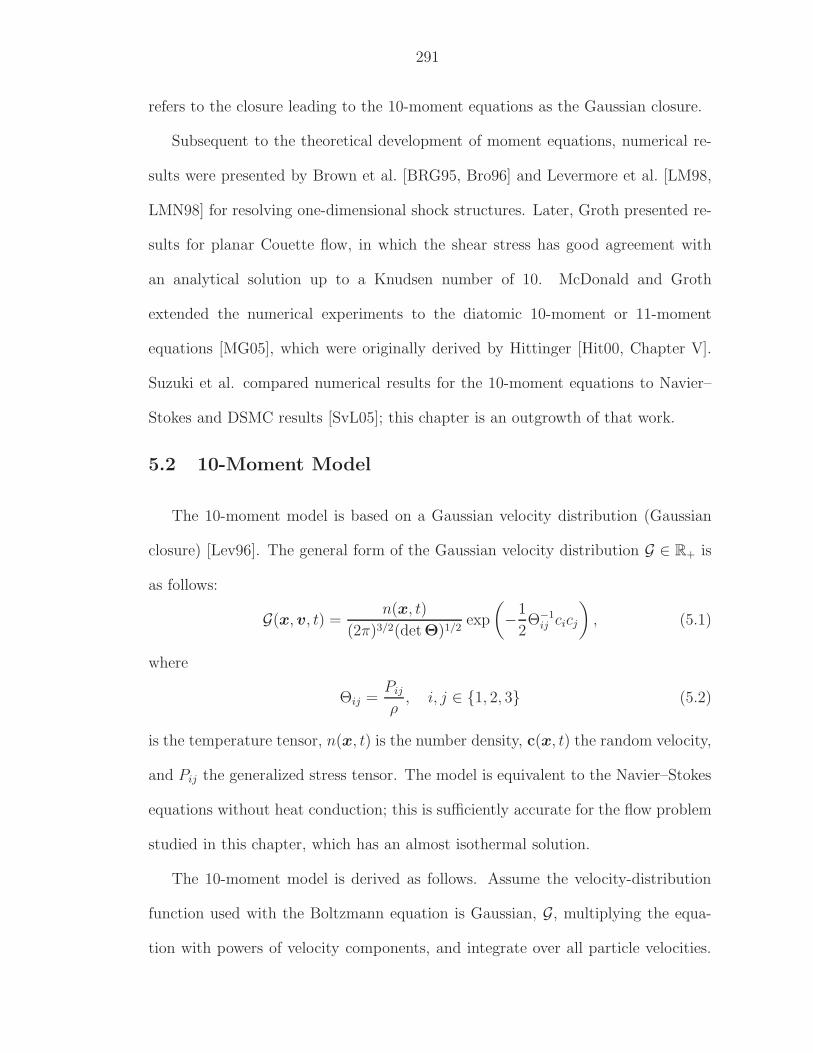
291
refers to the closure leading to the 10-moment equations as the Gaussian closure.
Subsequent to the theoretical development of moment equations, numerical re-
sults were presented by Brown et al. [BRG95, Bro96] and Levermore et al. [LM98,
LMN98] for resolving one-dimensional shock structures. Later, Groth presented re-
sults for planar Couette flow, in which the shear stress has good agreement with
an analytical solution up to a Knudsen number of 10. McDonald and Groth
extended the numerical experiments to the diatomic 10-moment or 11-moment
equations [MG05], which were originally derived by Hittinger [Hit00, Chapter V].
Suzuki et al. compared numerical results for the 10-moment equations to Navier–
Stokes and DSMC results [SvL05]; this chapter is an outgrowth of that work.
5.2 10-Moment Model
The 10-moment model is based on a Gaussian velocity distribution (Gaussian
closure) [Lev96]. The general form of the Gaussian velocity distribution G ∈ R+ is
as follows:
G(x, v, t) =n(x, t)
(2π)3/2(detΘ)1/2exp
(−1
2Θ−1
ij cicj
), (5.1)
where
Θij =Pij
ρ, i, j ∈ 1, 2, 3 (5.2)
is the temperature tensor, n(x, t) is the number density, c(x, t) the random velocity,
and Pij the generalized stress tensor. The model is equivalent to the Navier–Stokes
equations without heat conduction; this is sufficiently accurate for the flow problem
studied in this chapter, which has an almost isothermal solution.
The 10-moment model is derived as follows. Assume the velocity-distribution
function used with the Boltzmann equation is Gaussian, G, multiplying the equa-
tion with powers of velocity components, and integrate over all particle velocities.
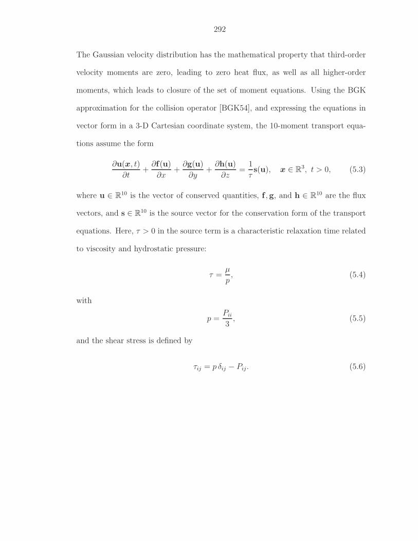
292
The Gaussian velocity distribution has the mathematical property that third-order
velocity moments are zero, leading to zero heat flux, as well as all higher-order
moments, which leads to closure of the set of moment equations. Using the BGK
approximation for the collision operator [BGK54], and expressing the equations in
vector form in a 3-D Cartesian coordinate system, the 10-moment transport equa-
tions assume the form
∂u(x, t)
∂t+
∂f(u)
∂x+
∂g(u)
∂y+
∂h(u)
∂z=
1
τs(u), x ∈ R
3, t > 0, (5.3)
where u ∈ R10 is the vector of conserved quantities, f , g, and h ∈ R10 are the flux
vectors, and s ∈ R10 is the source vector for the conservation form of the transport
equations. Here, τ > 0 in the source term is a characteristic relaxation time related
to viscosity and hydrostatic pressure:
τ =µ
p, (5.4)
with
p =Pii
3, (5.5)
and the shear stress is defined by
τij = p δij − Pij. (5.6)
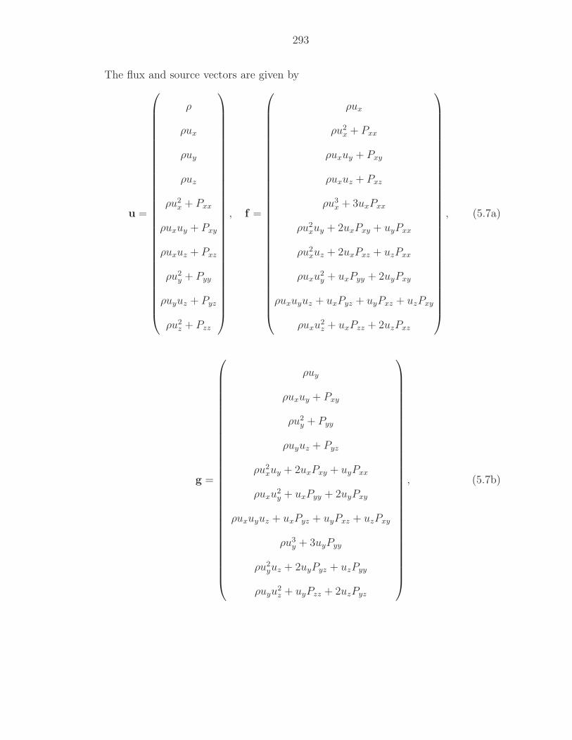
293
The flux and source vectors are given by
u =
ρ
ρux
ρuy
ρuz
ρu2x + Pxx
ρuxuy + Pxy
ρuxuz + Pxz
ρu2y + Pyy
ρuyuz + Pyz
ρu2z + Pzz
, f =
ρux
ρu2x + Pxx
ρuxuy + Pxy
ρuxuz + Pxz
ρu3x + 3uxPxx
ρu2xuy + 2uxPxy + uyPxx
ρu2xuz + 2uxPxz + uzPxx
ρuxu2y + uxPyy + 2uyPxy
ρuxuyuz + uxPyz + uyPxz + uzPxy
ρuxu2z + uxPzz + 2uzPxz
, (5.7a)
g =
ρuy
ρuxuy + Pxy
ρu2y + Pyy
ρuyuz + Pyz
ρu2xuy + 2uxPxy + uyPxx
ρuxu2y + uxPyy + 2uyPxy
ρuxuyuz + uxPyz + uyPxz + uzPxy
ρu3y + 3uyPyy
ρu2yuz + 2uyPyz + uzPyy
ρuyu2z + uyPzz + 2uzPyz
, (5.7b)
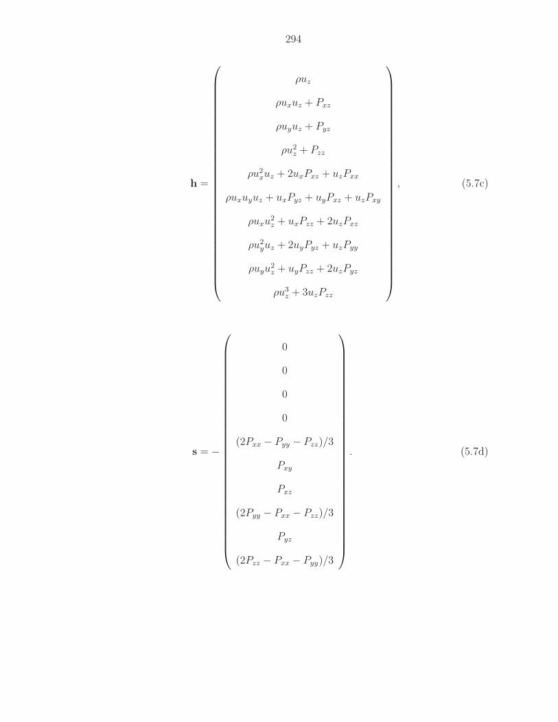
294
h =
ρuz
ρuxuz + Pxz
ρuyuz + Pyz
ρu2z + Pzz
ρu2xuz + 2uxPxz + uzPxx
ρuxuyuz + uxPyz + uyPxz + uzPxy
ρuxu2z + uxPzz + 2uzPxz
ρu2yuz + 2uyPyz + uzPyy
ρuyu2z + uyPzz + 2uzPyz
ρu3z + 3uzPzz
, (5.7c)
s = −
0
0
0
0
(2Pxx − Pyy − Pzz)/3
Pxy
Pxz
(2Pyy − Pxx − Pzz)/3
Pyz
(2Pzz − Pxx − Pyy)/3
. (5.7d)
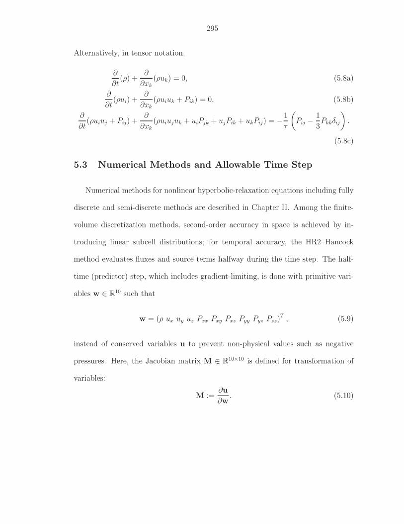
295
Alternatively, in tensor notation,
∂
∂t(ρ) +
∂
∂xk(ρuk) = 0, (5.8a)
∂
∂t(ρui) +
∂
∂xk(ρuiuk + Pik) = 0, (5.8b)
∂
∂t(ρuiuj + Pij) +
∂
∂xk
(ρuiujuk + uiPjk + ujPik + ukPij) = −1
τ
(Pij −
1
3Pkkδij
).
(5.8c)
5.3 Numerical Methods and Allowable Time Step
Numerical methods for nonlinear hyperbolic-relaxation equations including fully
discrete and semi-discrete methods are described in Chapter II. Among the finite-
volume discretization methods, second-order accuracy in space is achieved by in-
troducing linear subcell distributions; for temporal accuracy, the HR2–Hancock
method evaluates fluxes and source terms halfway during the time step. The half-
time (predictor) step, which includes gradient-limiting, is done with primitive vari-
ables w ∈ R10 such that
w = (ρ ux uy uz Pxx Pxy Pxz Pyy Pyz Pzz)T , (5.9)
instead of conserved variables u to prevent non-physical values such as negative
pressures. Here, the Jacobian matrix M ∈ R10×10 is defined for transformation of
variables:
M :=∂u
∂w. (5.10)
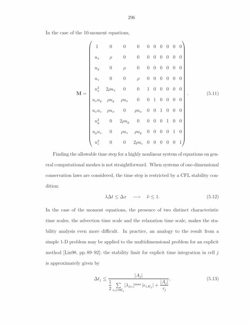
296
In the case of the 10-moment equations,
M =
1 0 0 0 0 0 0 0 0 0
ux ρ 0 0 0 0 0 0 0 0
uy 0 ρ 0 0 0 0 0 0 0
uz 0 0 ρ 0 0 0 0 0 0
u2x 2ρux 0 0 1 0 0 0 0 0
uxuy ρuy ρux 0 0 1 0 0 0 0
uxuz ρux 0 ρux 0 0 1 0 0 0
u2y 0 2ρuy 0 0 0 0 1 0 0
uyuz 0 ρuz ρuy 0 0 0 0 1 0
u2z 0 0 2ρuz 0 0 0 0 0 1
. (5.11)
Finding the allowable time step for a highly nonlinear system of equations on gen-
eral computational meshes is not straightforward. When systems of one-dimensional
conservation laws are considered, the time step is restricted by a CFL stability con-
dition:
λ∆t ≤ ∆x −→ ν ≤ 1. (5.12)
In the case of the moment equations, the presence of two distinct characteristic
time scales, the advection time scale and the relaxation time scale, makes the sta-
bility analysis even more difficult. In practice, an analogy to the result from a
simple 1-D problem may be applied to the multidimensional problem for an explicit
method [Lin98, pp. 89–92]; the stability limit for explicit time integration in cell j
is approximately given by
∆tj ≤|Aj|
1
2
∑ei∈∂Kj
|λjei|max |ei,Kj
| + |Aj|τj
, (5.13)
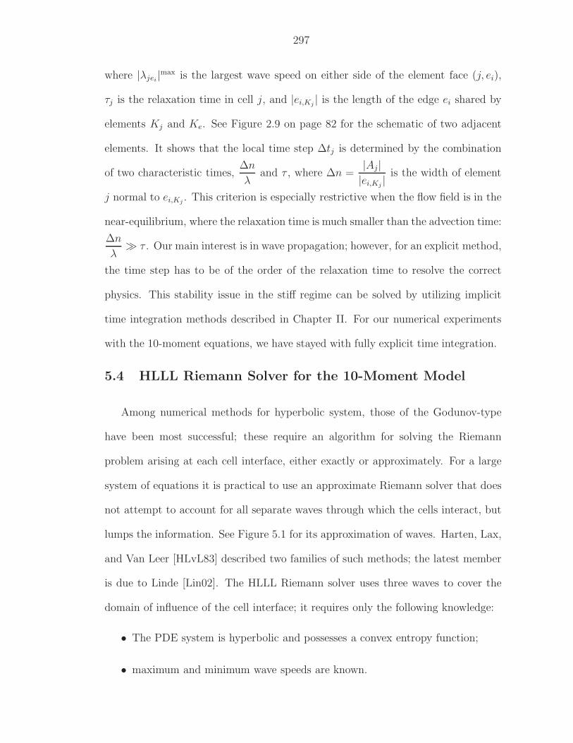
297
where |λjei|max is the largest wave speed on either side of the element face (j, ei),
τj is the relaxation time in cell j, and |ei,Kj| is the length of the edge ei shared by
elements Kj and Ke. See Figure 2.9 on page 82 for the schematic of two adjacent
elements. It shows that the local time step ∆tj is determined by the combination
of two characteristic times,∆n
λand τ , where ∆n =
|Aj||ei,Kj
| is the width of element
j normal to ei,Kj. This criterion is especially restrictive when the flow field is in the
near-equilibrium, where the relaxation time is much smaller than the advection time:
∆n
λ≫ τ . Our main interest is in wave propagation; however, for an explicit method,
the time step has to be of the order of the relaxation time to resolve the correct
physics. This stability issue in the stiff regime can be solved by utilizing implicit
time integration methods described in Chapter II. For our numerical experiments
with the 10-moment equations, we have stayed with fully explicit time integration.
5.4 HLLL Riemann Solver for the 10-Moment Model
Among numerical methods for hyperbolic system, those of the Godunov-type
have been most successful; these require an algorithm for solving the Riemann
problem arising at each cell interface, either exactly or approximately. For a large
system of equations it is practical to use an approximate Riemann solver that does
not attempt to account for all separate waves through which the cells interact, but
lumps the information. See Figure 5.1 for its approximation of waves. Harten, Lax,
and Van Leer [HLvL83] described two families of such methods; the latest member
is due to Linde [Lin02]. The HLLL Riemann solver uses three waves to cover the
domain of influence of the cell interface; it requires only the following knowledge:
• The PDE system is hyperbolic and possesses a convex entropy function;
• maximum and minimum wave speeds are known.
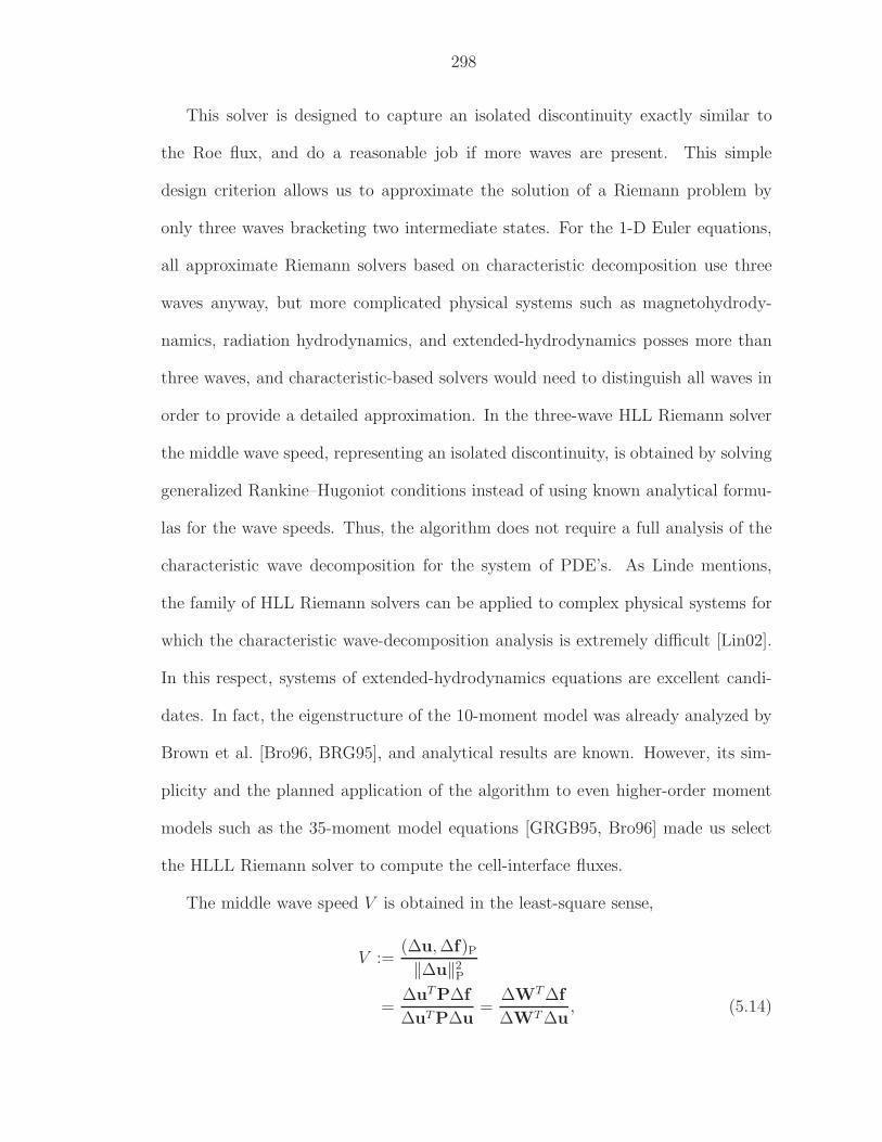
298
This solver is designed to capture an isolated discontinuity exactly similar to
the Roe flux, and do a reasonable job if more waves are present. This simple
design criterion allows us to approximate the solution of a Riemann problem by
only three waves bracketing two intermediate states. For the 1-D Euler equations,
all approximate Riemann solvers based on characteristic decomposition use three
waves anyway, but more complicated physical systems such as magnetohydrody-
namics, radiation hydrodynamics, and extended-hydrodynamics posses more than
three waves, and characteristic-based solvers would need to distinguish all waves in
order to provide a detailed approximation. In the three-wave HLL Riemann solver
the middle wave speed, representing an isolated discontinuity, is obtained by solving
generalized Rankine–Hugoniot conditions instead of using known analytical formu-
las for the wave speeds. Thus, the algorithm does not require a full analysis of the
characteristic wave decomposition for the system of PDE’s. As Linde mentions,
the family of HLL Riemann solvers can be applied to complex physical systems for
which the characteristic wave-decomposition analysis is extremely difficult [Lin02].
In this respect, systems of extended-hydrodynamics equations are excellent candi-
dates. In fact, the eigenstructure of the 10-moment model was already analyzed by
Brown et al. [Bro96, BRG95], and analytical results are known. However, its sim-
plicity and the planned application of the algorithm to even higher-order moment
models such as the 35-moment model equations [GRGB95, Bro96] made us select
the HLLL Riemann solver to compute the cell-interface fluxes.
The middle wave speed V is obtained in the least-square sense,
V :=(∆u, ∆f)P
‖∆u‖2P
=∆uT P∆f
∆uTP∆u=
∆WT ∆f
∆WT ∆u, (5.14)
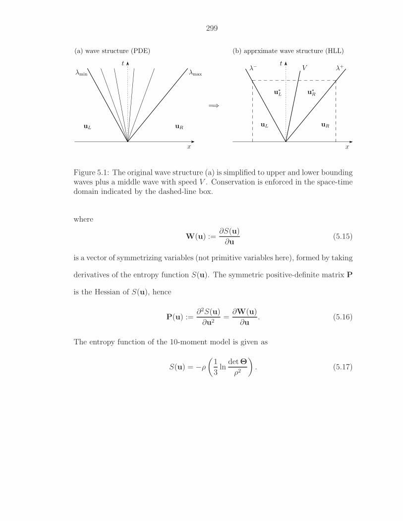
299
x
t
x
t
uL uRuRuL
u∗L u∗
R
Vλ− λ+
λmin λmax
=⇒
(a) wave structure (PDE) (b) apprximate wave structure (HLL)
Figure 5.1: The original wave structure (a) is simplified to upper and lower boundingwaves plus a middle wave with speed V . Conservation is enforced in the space-timedomain indicated by the dashed-line box.
where
W(u) :=∂S(u)
∂u(5.15)
is a vector of symmetrizing variables (not primitive variables here), formed by taking
derivatives of the entropy function S(u). The symmetric positive-definite matrix P
is the Hessian of S(u), hence
P(u) :=∂2S(u)
∂u2=
∂W(u)
∂u. (5.16)
The entropy function of the 10-moment model is given as
S(u) = −ρ
(1
3ln
detΘ
ρ2
). (5.17)
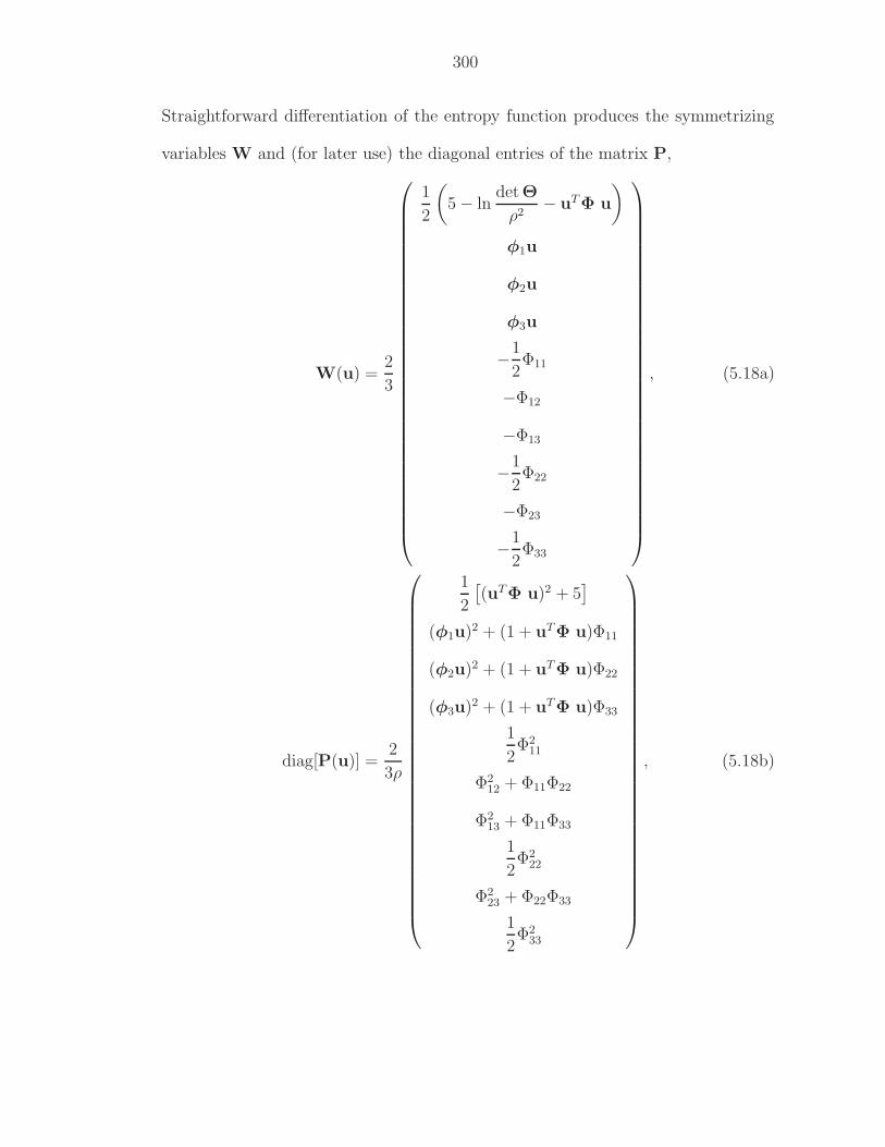
300
Straightforward differentiation of the entropy function produces the symmetrizing
variables W and (for later use) the diagonal entries of the matrix P,
W(u) =2
3
1
2
(5 − ln
detΘ
ρ2− uT Φ u
)
φ1u
φ2u
φ3u
−1
2Φ11
−Φ12
−Φ13
−1
2Φ22
−Φ23
−1
2Φ33
, (5.18a)
diag[P(u)] =2
3ρ
1
2
[(uTΦ u)2 + 5
]
(φ1u)2 + (1 + uTΦ u)Φ11
(φ2u)2 + (1 + uTΦ u)Φ22
(φ3u)2 + (1 + uTΦ u)Φ33
1
2Φ2
11
Φ212 + Φ11Φ22
Φ213 + Φ11Φ33
1
2Φ2
22
Φ223 + Φ22Φ33
1
2Φ2
33
, (5.18b)
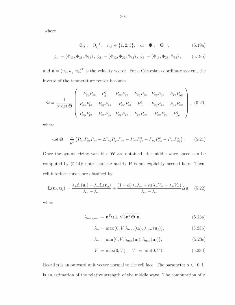
301
where
Φij := Θ−1ij , i, j ∈ 1, 2, 3, or Φ := Θ−1, (5.19a)
φ1 := (Φ11, Φ21, Φ31) , φ2 := (Φ12, Φ22, Φ32) , φ3 := (Φ13, Φ23, Φ33) , (5.19b)
and u = (ux, uy, uz)T is the velocity vector. For a Cartesian coordinate system, the
inverse of the temperature tensor becomes
Φ =1
ρ2 detΘ
PyyPzz − P 2yz PxzPyz − PxyPzz PxyPyz − PxzPyy
PxzPyz − PxyPzz PxxPzz − P 2xz PxyPxz − PyzPxx
PxyPyz − PxzPyy PxyPxz − PyzPxx PxxPyy − P 2xy
, (5.20)
where
detΘ =1
ρ3
(PxxPyyPzz + 2PxyPyzPxz − PxxP
2yz − PyyP
2xz − PzzP
2xy
). (5.21)
Once the symmetrizing variables W are obtained, the middle wave speed can be
computed by (5.14); note that the matrix P is not explicitly needed here. Then,
cell-interface fluxes are obtained by
fn(ui,uj) =λ+fn(ui) − λ−fn(uj)
λ+ − λ−+
(1 − α)λ−λ+ + α(λ−V+ + λ+V−)
λ+ − λ−∆u, (5.22)
where
λmax,min = nTu±√
3nTΘ n, (5.23a)
λ+ = max(0, V, λmax(ui), λmax(uj)
), (5.23b)
λ− = min(0, V, λmin(ui), λmin(uj)
), (5.23c)
V+ = max(0, V ), V− = min(0, V ). (5.23d)
Recall n is an outward unit vector normal to the cell face. The parameter α ∈ [ 0, 1 ]
is an estimation of the relative strength of the middle wave. The computation of α
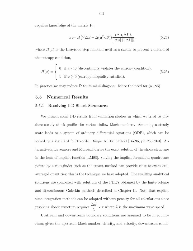
302
requires knowledge of the matrix P,
α := H(V ∆S − ∆(nT uS)
) (∆u, ∆f)2P
‖∆u‖2P‖∆f‖2
P
, (5.24)
where H(x) is the Heaviside step function used as a switch to prevent violation of
the entropy condition,
H(x) =
0 if x < 0 (discontinuity violates the entropy condition),
1 if x ≥ 0 (entropy inequality satisfied).
(5.25)
In practice we may reduce P to its main diagonal, hence the need for (5.18b).
5.5 Numerical Results
5.5.1 Resolving 1-D Shock Structures
We present some 1-D results from validation studies in which we tried to pro-
duce steady shock profiles for various inflow Mach numbers. Assuming a steady
state leads to a system of ordinary differential equations (ODE), which can be
solved by a standard fourth-order Runge–Kutta method [Bro96, pp. 256–263]. Al-
ternatively, Levermore and Morokoff derive the exact solution of the shock structure
in the form of implicit function [LM98]. Solving the implicit formula at quadrature
points by a root-finder such as the secant method can provide close-to-exact cell-
averaged quantities; this is the technique we have adopted. The resulting analytical
solutions are compared with solutions of the PDE’s obtained by the finite-volume
and discontinuous Galerkin methods described in Chapter II. Note that explicit
time-integration methods can be adopted without penalty for all calculations since
resolving shock structure requires∆h
λ∼ τ where λ is the maximum wave speed.
Upstream and downstream boundary conditions are assumed to be in equilib-
rium; given the upstream Mach number, density, and velocity, downstream condi-
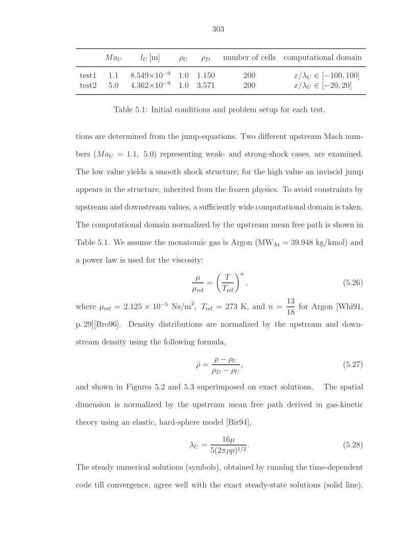
303
MaU lU [m] ρU ρD number of cells computational domain
test1 1.1 8.549×10⁻⁹ 1.0 1.150 200 x/λU ∈ [−100, 100]test2 5.0 4.362×10⁻⁹ 1.0 3.571 200 x/λU ∈ [−20, 20]
Table 5.1: Initial conditions and problem setup for each test.
tions are determined from the jump-equations. Two different upstream Mach num-
bers (MaU = 1.1, 5.0) representing weak- and strong-shock cases, are examined.
The low value yields a smooth shock structure; for the high value an inviscid jump
appears in the structure, inherited from the frozen physics. To avoid constraints by
upstream and downstream values, a sufficiently wide computational domain is taken.
The computational domain normalized by the upstream mean free path is shown in
Table 5.1. We assume the monatomic gas is Argon (MWAr = 39.948 kg/kmol) and
a power law is used for the viscosity:
µ
µref
=
(T
Tref
)n
, (5.26)
where µref = 2.125 × 10⁻⁵ Ns/m2, Tref = 273 K, and n =13
18for Argon [Whi91,
p. 29][Bro96]. Density distributions are normalized by the upstream and down-
stream density using the following formula,
ρ =ρ − ρU
ρD − ρU, (5.27)
and shown in Figures 5.2 and 5.3 superimposed on exact solutions. The spatial
dimension is normalized by the upstream mean free path derived in gas-kinetic
theory using an elastic, hard-sphere model [Bir94],
λU =16µ
5(2πρp)1/2. (5.28)
The steady numerical solutions (symbols), obtained by running the time-dependent
code till convergence, agree well with the exact steady-state solutions (solid line).
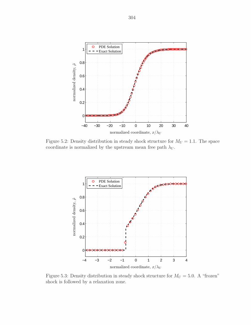
304
−40 −30 −20 −10 0 10 20 30 40
0
0.2
0.4
0.6
0.8
1
PDE SolutionExact Solution
normalized coordinate, x/λU
norm
alize
dden
sity
,ρ
Figure 5.2: Density distribution in steady shock structure for MU = 1.1. The spacecoordinate is normalized by the upstream mean free path λU .
−4 −3 −2 −1 0 1 2 3 4
0
0.2
0.4
0.6
0.8
1
PDE SolutionExact Solution
normalized coordinate, x/λU
norm
alize
dden
sity
,ρ
Figure 5.3: Density distribution in steady shock structure for MU = 5.0. A “frozen”shock is followed by a relaxation zone.
305
In Table 5.2, density errors computed for a sequence of grids when MU = 1.1 are
tabulated; their convergence rates demonstrate the second-order spatial accuracy of
the HR2–RK2, HR2–Hancock, and DG(1)–RK2 methods, and first-order accuracy
for the HR1 method. The Runge–Kutta time-integration methods do not affect
the accuracy of the converged steady solutions; the Hancock scheme does yield
dependence on the CFL numbers used (not tested). Nevertheless, the error-norms
of the HR2–RK2 and HR2–Hancock methods for the same grid are almost identical.
The error norms against degrees of freedom and CPU time are also plotted in
Figure 5.4. It shows the higher accuracy of the DG(1) spatial discretization over
HR2 methods. Owing to the high accuracy of the DG(1) method, it is also the most
efficient among all methods.
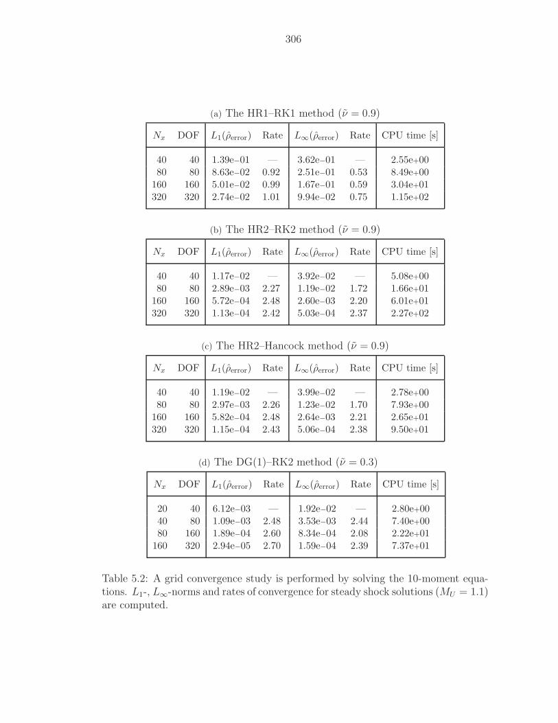
306
(a) The HR1–RK1 method (ν = 0.9)
Nx DOF L1(ρerror) Rate L∞(ρerror) Rate CPU time [s]
40 40 1.39e−01 — 3.62e−01 — 2.55e+0080 80 8.63e−02 0.92 2.51e−01 0.53 8.49e+00
160 160 5.01e−02 0.99 1.67e−01 0.59 3.04e+01320 320 2.74e−02 1.01 9.94e−02 0.75 1.15e+02
(b) The HR2–RK2 method (ν = 0.9)
Nx DOF L1(ρerror) Rate L∞(ρerror) Rate CPU time [s]
40 40 1.17e−02 — 3.92e−02 — 5.08e+0080 80 2.89e−03 2.27 1.19e−02 1.72 1.66e+01
160 160 5.72e−04 2.48 2.60e−03 2.20 6.01e+01320 320 1.13e−04 2.42 5.03e−04 2.37 2.27e+02
(c) The HR2–Hancock method (ν = 0.9)
Nx DOF L1(ρerror) Rate L∞(ρerror) Rate CPU time [s]
40 40 1.19e−02 — 3.99e−02 — 2.78e+0080 80 2.97e−03 2.26 1.23e−02 1.70 7.93e+00
160 160 5.82e−04 2.48 2.64e−03 2.21 2.65e+01320 320 1.15e−04 2.43 5.06e−04 2.38 9.50e+01
(d) The DG(1)–RK2 method (ν = 0.3)
Nx DOF L1(ρerror) Rate L∞(ρerror) Rate CPU time [s]
20 40 6.12e−03 — 1.92e−02 — 2.80e+0040 80 1.09e−03 2.48 3.53e−03 2.44 7.40e+0080 160 1.89e−04 2.60 8.34e−04 2.08 2.22e+01
160 320 2.94e−05 2.70 1.59e−04 2.39 7.37e+01
Table 5.2: A grid convergence study is performed by solving the 10-moment equa-tions. L1-, L∞-norms and rates of convergence for steady shock solutions (MU = 1.1)are computed.
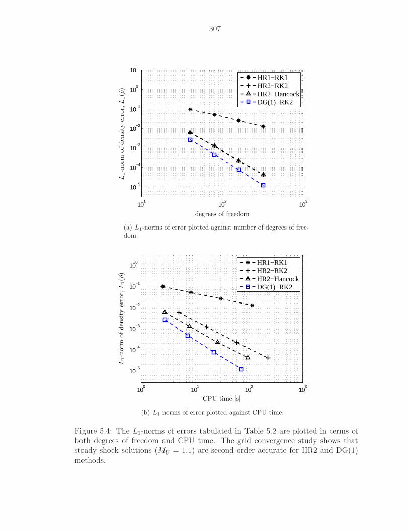
307
101
102
103
10−5
10−4
10−3
10−2
10−1
100
101
HR1−RK1HR2−RK2HR2−HancockDG(1)−RK2
degrees of freedom
L1-n
orm
ofden
sity
erro
r,L
1(ρ
)
(a) L1-norms of error plotted against number of degrees of free-dom.
100
101
102
103
10−5
10−4
10−3
10−2
10−1
100
HR1−RK1HR2−RK2HR2−HancockDG(1)−RK2
CPU time [s]
L1-n
orm
ofden
sity
erro
r,L
1(ρ
)
(b) L1-norms of error plotted against CPU time.
Figure 5.4: The L1-norms of errors tabulated in Table 5.2 are plotted in terms ofboth degrees of freedom and CPU time. The grid convergence study shows thatsteady shock solutions (MU = 1.1) are second order accurate for HR2 and DG(1)methods.
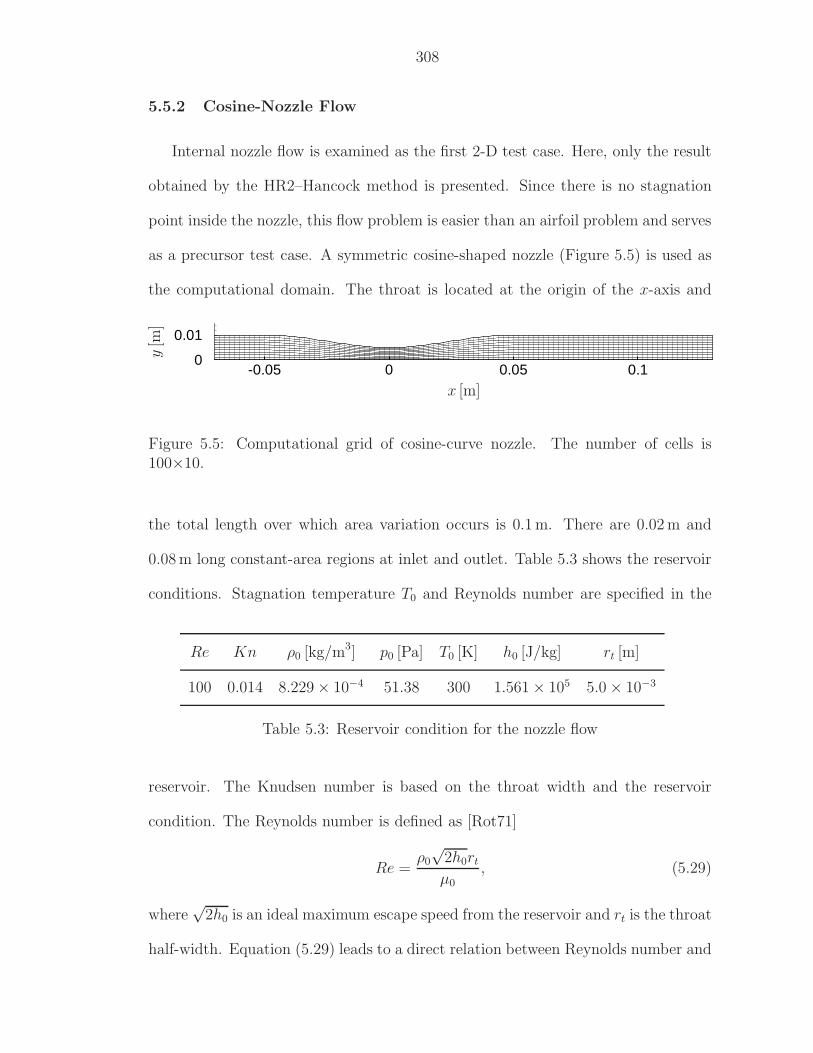
308
5.5.2 Cosine-Nozzle Flow
Internal nozzle flow is examined as the first 2-D test case. Here, only the result
obtained by the HR2–Hancock method is presented. Since there is no stagnation
point inside the nozzle, this flow problem is easier than an airfoil problem and serves
as a precursor test case. A symmetric cosine-shaped nozzle (Figure 5.5) is used as
the computational domain. The throat is located at the origin of the x-axis and
-0.05 0 0.05 0.10
0.01
x [m]
y[m
]
Figure 5.5: Computational grid of cosine-curve nozzle. The number of cells is100×10.
the total length over which area variation occurs is 0.1 m. There are 0.02 m and
0.08 m long constant-area regions at inlet and outlet. Table 5.3 shows the reservoir
conditions. Stagnation temperature T0 and Reynolds number are specified in the
Re Kn ρ0 [kg/m3] p0 [Pa] T0 [K] h0 [J/kg] rt [m]
100 0.014 8.229 × 10⁻⁴ 51.38 300 1.561 × 10⁵ 5.0 × 10⁻³
Table 5.3: Reservoir condition for the nozzle flow
reservoir. The Knudsen number is based on the throat width and the reservoir
condition. The Reynolds number is defined as [Rot71]
Re =ρ0
√2h0rt
µ0, (5.29)
where√
2h0 is an ideal maximum escape speed from the reservoir and rt is the throat
half-width. Equation (5.29) leads to a direct relation between Reynolds number and
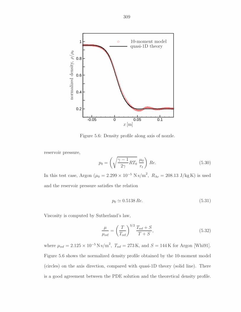
309
-0.05 0 0.05 0.1
0.2
0.4
0.6
0.8
1
x [m]
nor
mal
ized
den
sity
,ρ/ρ
0
10-moment modelquasi-1D theory
Figure 5.6: Density profile along axis of nozzle.
reservoir pressure,
p0 =
(√γ − 1
2γRT0
µ0
rt
)Re. (5.30)
In this test case, Argon (µ0 = 2.299 × 10⁻⁵ Ns/m2, RAr = 208.13 J/kgK) is used
and the reservoir pressure satisfies the relation
p0 ≃ 0.5138 Re. (5.31)
Viscosity is computed by Sutherland’s law,
µ
µref=
(T
Tref
)3/2Tref + S
T + S, (5.32)
where µref = 2.125 × 10⁻⁵ Ns/m2, Tref = 273 K, and S = 144 K for Argon [Whi91].
Figure 5.6 shows the normalized density profile obtained by the 10-moment model
(circles) on the axis direction, compared with quasi-1D theory (solid line). There
is a good agreement between the PDE solution and the theoretical density profile.
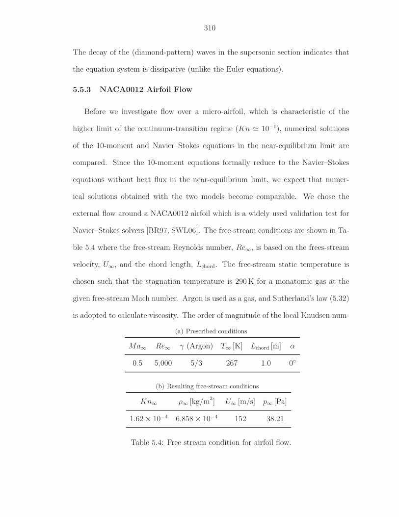
310
The decay of the (diamond-pattern) waves in the supersonic section indicates that
the equation system is dissipative (unlike the Euler equations).
5.5.3 NACA0012 Airfoil Flow
Before we investigate flow over a micro-airfoil, which is characteristic of the
higher limit of the continuum-transition regime (Kn ≃ 10−1), numerical solutions
of the 10-moment and Navier–Stokes equations in the near-equilibrium limit are
compared. Since the 10-moment equations formally reduce to the Navier–Stokes
equations without heat flux in the near-equilibrium limit, we expect that numer-
ical solutions obtained with the two models become comparable. We chose the
external flow around a NACA0012 airfoil which is a widely used validation test for
Navier–Stokes solvers [BR97, SWL06]. The free-stream conditions are shown in Ta-
ble 5.4 where the free-stream Reynolds number, Re∞, is based on the frees-stream
velocity, U∞, and the chord length, Lchord. The free-stream static temperature is
chosen such that the stagnation temperature is 290K for a monatomic gas at the
given free-stream Mach number. Argon is used as a gas, and Sutherland’s law (5.32)
is adopted to calculate viscosity. The order of magnitude of the local Knudsen num-
(a) Prescribed conditions
Ma∞ Re∞ γ (Argon) T∞ [K] Lchord [m] α
0.5 5,000 5/3 267 1.0 0
(b) Resulting free-stream conditions
Kn∞ ρ∞ [kg/m3] U∞ [m/s] p∞ [Pa]
1.62 × 10⁻⁴ 6.858 × 10⁻⁴ 152 38.21
Table 5.4: Free stream condition for airfoil flow.
311
ber in a boundary layer is approximately
Kn ∼ Ma∞
Reδ∼ Ma∞√
Re∞= 7.1 × 10⁻³, (5.33)
where δ is the boundary layer thickness [GeH99]. Hence, the flow in the boundary
layer is at the lower end of the continuum-transition regime (cf. Table 1.1 on
page 10).
The HR2–Hancock method is applied to solve the 10-moment equations, and
HR2–RK is used for the Navier–Stokes equations. Both methods employ a C-type
grid composed by 120 × 76 cells. A typical finite-volume discretization of the
Navier–Stokes equations consists of two parts: the inviscid flux obtained by a Rie-
mann solver, and the viscous flux by central differencing. Here, we omit the descrip-
tion of discretization methods for the viscous-flux terms. Details of the implemen-
tation, particularly for a quadrilateral grid, can be found in [Fle91, pp. 105–110].
Since our Navier–Stokes solver is explicit, the stable time step becomes a function
of both the advective time-scale,h
λ, and the viscous time-scale,
ρh2
µ, where h is a
typical cell size. Based on the 1-D linear stability analysis for an advection-diffusion
equation, and following the notation used in (5.13) on page 296, the stable time step
for the 2-D Navier–Stokes equations can be written as
∆tj ≤ min
[|Aj|c1
+c2
c21
,
(c1
|Aj|+
c2
|Aj|2)−1
], (5.34)
where
c1 =1
2
∑
ei∈∂Kj
|λjei|max |ei,Kj
|, (5.35a)
c2 =∑
ei∈∂Kj
µjei|ei,Kj
|2ρjei
. (5.35b)
See also Figure 2.7 on page 68 for the notation.
312
For a finite-volume method, in order to achieve second-order accuracy, the re-
construction of flow gradients in the each cell is required. Typically, either com-
puting a Green–Gauss contour-integral, or solving a least-square problem provides
the gradients; these procedure require all neighboring cells of the cell of interest.
When gradients at cells abutting the solid wall are computed, ghost cells are in-
troduced. Along the solid boundary, the non-slip boundary condition is employed.
Let (ucj, vcj) be the velocity vector associated with the centroid xcj of the cell i,
(ucg, vcg) the velocity vector at the centroid xcg of the ghost cell, and Q the rotation
matrix defined by
Q :=
nx sx 0
ny sy 0
0 0 1
=
nx ny 0
ny −nx 0
0 0 1
, (5.36)
where n = (nx, ny, 0) the outward unit vector normal to the wall, and s = (sx, sy, 0)
the unit vector tangential to the wall (see Figure 5.7); then, the non-slip boundary
condition leads to the velocity at the centroid of the ghost cell as follows:
(ucg, vcg, 0)Q = −(ucj, vcj, 0)Q −→ (ucg, vcg) = (−ucj,−vcj). (5.37)
This condition enforces zero velocity at the wall surface: (us, vs) = 0. As to the
density and pressure, owing to the assumption,∂p
∂n≈ 0, inside the boundary layer,
and the adiabatic wall,∂T
∂n= 0, together with the equation of state, p = ρRT , we
have
∂ρ
∂n≈ 0,
∂p
∂n≈ 0. (5.38)
Hence, the density and pressure in the ghost cell can be prescribed such that
ρcg = ρcj, and pcg = pcj. (5.39)
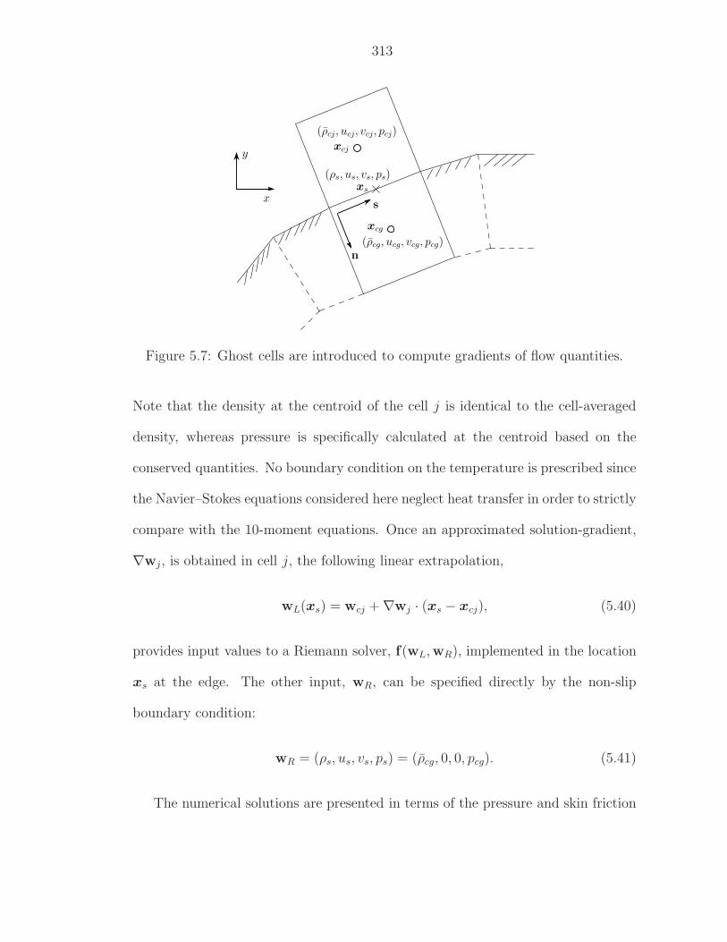
313
xcj
xcg
(ρcj , ucj, vcj, pcj)
(ρcg, ucg, vcg, pcg)
xs
n
s
(ρs, us, vs, ps)
x
y
Figure 5.7: Ghost cells are introduced to compute gradients of flow quantities.
Note that the density at the centroid of the cell j is identical to the cell-averaged
density, whereas pressure is specifically calculated at the centroid based on the
conserved quantities. No boundary condition on the temperature is prescribed since
the Navier–Stokes equations considered here neglect heat transfer in order to strictly
compare with the 10-moment equations. Once an approximated solution-gradient,
∇wj, is obtained in cell j, the following linear extrapolation,
wL(xs) = wcj + ∇wj · (xs − xcj), (5.40)
provides input values to a Riemann solver, f(wL,wR), implemented in the location
xs at the edge. The other input, wR, can be specified directly by the non-slip
boundary condition:
wR = (ρs, us, vs, ps) = (ρcg, 0, 0, pcg). (5.41)
The numerical solutions are presented in terms of the pressure and skin friction
314
coefficients defined by
Cp(x) :=p(x) − p∞1
2ρ∞U2
∞
=2
γMa2∞
(p(x)
p∞− 1
), (5.42a)
Cf(x) :=τs(x)
1
2ρ∞U2
∞
, (5.42b)
along the surface of the airfoil; the pressure in the 10-moment model is given by (5.5).
Here, the dimensionless x-coordinate is defined by x :=x
Lchord
, and x = 0, 1 cor-
respond to the leading and trailing edges, respectively. The tangential shear stress
along the wall, τs, can be directly computed with the 10-moment equations by
rotating the stress tensor P in x-,y-coordinates to P′ in n-,s-coordinates:
P′ =
Pnn Pns Pnz
Psn Pss Psz
Pzn Pzs Pzz
:= QTPQ, (5.43)
yielding
τs = −Pns
= (Pyy − Pxx)nxny + Pxy(n2x − n2
y). (5.44)
In the case of the Navier–Stokes equations, the tangential shear stress is obtained
by using the relation (5.6) on page 292, yielding
τs = (τxx − τyy)nxny + τxy(n2y − n2
x), (5.45)
where the components of the shear stress tensor are obtained by the following
Navier–Stokes constitutive laws:
τxx = µ
[2∂u
∂x− 2
3
(∂u
∂x+
∂v
∂y
)], (5.46a)
τyy = µ
[2∂v
∂y− 2
3
(∂u
∂x+
∂v
∂y
)], (5.46b)
τxy = µ
(∂u
∂y+
∂v
∂x
). (5.46c)
315
Figure 5.8(a) shows the excellent agreement of pressure coefficients between
the 10-moment and Navier–Stokes solutions. The theoretical maximum pressure-
coefficient for (Ma∞, γ) = (0.5, 5/3) is obtained by the isentropic relation:
p0
p∞≃ 1.2215 −→ (Cp)max = 1.0634. (5.47)
Both solutions slightly overshoot the theoretical maximum pressure coefficient at
the cell adjacent to the leading edge. In Figure 5.8(b), we observe that the 10-
moment model predicts a lower peak of the skin-friction coefficient, (Cf)max. This
is somewhat surprising since we expect the 10-moment equations to predict the shear
stresses more accurate because they are flow variables. This might be traced back to
the relatively high Knudsen number in the boundary layer shown in (5.33). Since the
flow is not completely in the continuum flow regime (Kn ≤ 10−3), nonequilibrium
effects described by the 10-moment equations in the boundary layer could predict
different surface values as computed to the Navier–Stokes equations.
The density profiles along the centerline of the airfoil are shown in Figure 5.9.
Both models agree well except near the stagnation point; the Navier–Stokes code
predicts slightly higher density values. The isentropic relation provides the theoret-
ical maximum stagnation density,
ρ0
ρ∞
≃ 1.1276. (5.48)
Unlike the pressure coefficients, the maximum densities predicted by both models
stay clearly lower that the isentropic stagnation density. While the pressure ap-
proximately remains constant across the boundary layer near the stagnation point,
the density is affected by the local dissipation. Insufficient grid resolution near the
stagnation could lead to lower predicted density values.
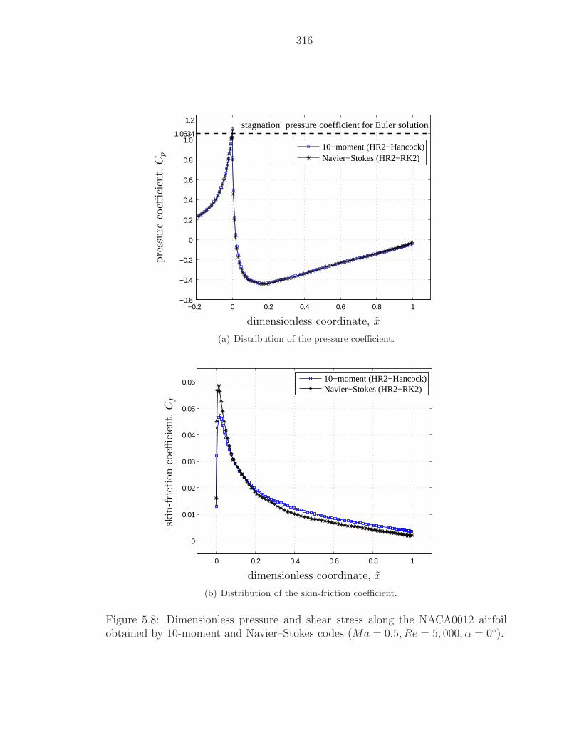
316
−0.2 0 0.2 0.4 0.6 0.8 1−0.6
−0.4
−0.2
0
0.2
0.4
0.6
0.8
1.0 1.0634
1.2
stagnation−pressure coefficient for Euler solution
10−moment (HR2−Hancock)Navier−Stokes (HR2−RK2)
dimensionless coordinate, x
pre
ssure
coeffi
cien
t,C
p
(a) Distribution of the pressure coefficient.
0 0.2 0.4 0.6 0.8 1
0
0.01
0.02
0.03
0.04
0.05
0.06
10−moment (HR2−Hancock)Navier−Stokes (HR2−RK2)
dimensionless coordinate, x
skin
-fri
ctio
nco
effici
ent,
Cf
(b) Distribution of the skin-friction coefficient.
Figure 5.8: Dimensionless pressure and shear stress along the NACA0012 airfoilobtained by 10-moment and Navier–Stokes codes (Ma = 0.5, Re = 5, 000, α = 0).
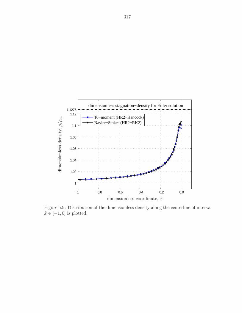
317
−1 −0.8 −0.6 −0.4 −0.2 0.0
1
1.02
1.04
1.06
1.08
1.1
1.12 1.1276
dimensionless stagnation−density for Euler solution
10−moment (HR2−Hancock)Navier−Stokes (HR2−RK2)
dimensionless coordinate, x
dim
ensi
onle
ssden
sity
,ρ/ρ
∞
Figure 5.9: Distribution of the dimensionless density along the centerline of intervalx ∈ [−1, 0] is plotted.
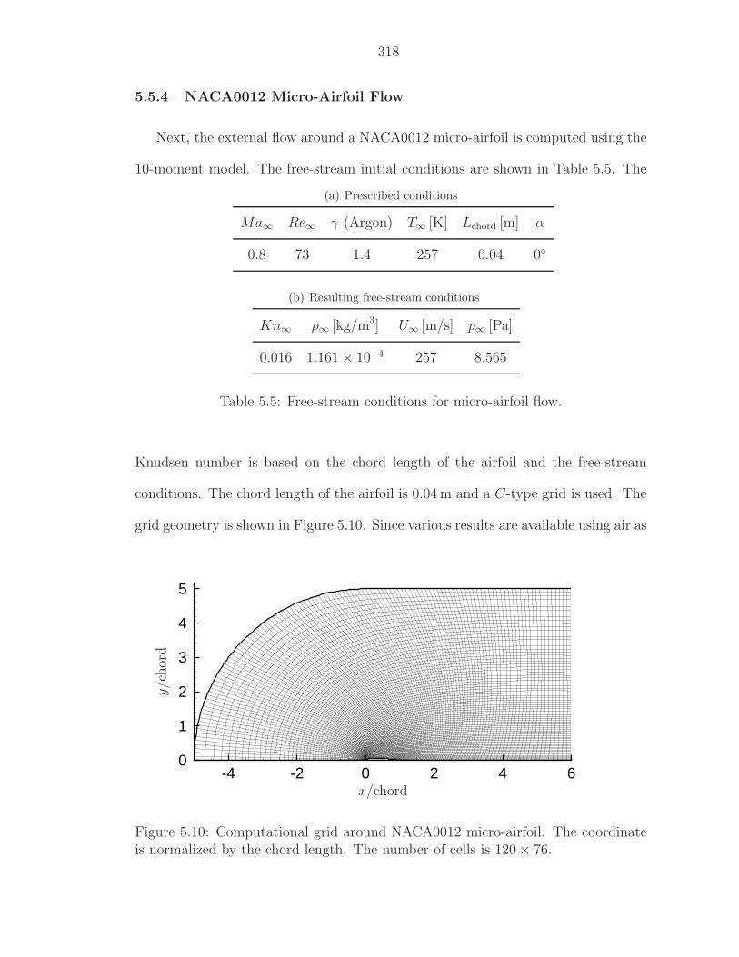
318
5.5.4 NACA0012 Micro-Airfoil Flow
Next, the external flow around a NACA0012 micro-airfoil is computed using the
10-moment model. The free-stream initial conditions are shown in Table 5.5. The
(a) Prescribed conditions
Ma∞ Re∞ γ (Argon) T∞ [K] Lchord [m] α
0.8 73 1.4 257 0.04 0
(b) Resulting free-stream conditions
Kn∞ ρ∞ [kg/m3] U∞ [m/s] p∞ [Pa]
0.016 1.161 × 10⁻⁴ 257 8.565
Table 5.5: Free-stream conditions for micro-airfoil flow.
Knudsen number is based on the chord length of the airfoil and the free-stream
conditions. The chord length of the airfoil is 0.04 m and a C-type grid is used. The
grid geometry is shown in Figure 5.10. Since various results are available using air as
-4 -2 0 2 4 60
1
2
3
4
5
x/chord
y/c
hor
d
Figure 5.10: Computational grid around NACA0012 micro-airfoil. The coordinateis normalized by the chord length. The number of cells is 120 × 76.
319
the gas, we also assume the gas is air (MWAir = 28.966 kg/kmol), even though the
10-moment model assumes a monatomic gas. Viscosity is computed by Sutherland’s
law (5.32) where µref = 1.716 × 10⁻⁵ Ns/m2, Tref = 273 K, and S = 111 K for Air.
Hittinger has added rotational degrees of freedom to the system, leading to an
11-moment model for a diatomic gas [Hit00]; we have not used this model. The 10-
moment equation implicitly assume γ = 5/3, rather than γ = 1.4; for the density
results presented below this hardly makes a difference (see below).
In the continuum-transition regime where Kn ∈ [10−3, 10−1], the flow on the
wall has a finite velocity. This slip velocity is approximated by Maxwell’s first-order
slip boundary condition,
ugas − uwall =2 − σ
σ
λ
µτs, (5.49)
where σ is an accommodation coefficient, λ is the mean free path, µ is the viscos-
ity, and τs is the tangential shear stress. The flow toward the wall is assumed to
have a Maxwellian velocity distribution. At the airfoil, completely diffuse molecu-
lar reflection is assumed in formulating the boundary condition for both methods
(achieved by setting σ = 1). The tangential shear stress is obtained by (5.45) for
the 10-moment equations. For instance, the slip velocity on a plane wall parallel to
the x-direction, n = (0, 1), is obtained by
ugas − uwall =2 − σ
σ
λ
µ(−Pxy). (5.50)
Furthermore, inserting the mean free path based on the Chapman–Enskog distri-
bution function [VK86, p. 414],
λ = µ
√π
2ρp, (5.51)
into the above equation leads to the following slip velocity:
ugas − uwall =2 − σ
σ
√π
2
(−Pxy)√ρp
, (5.52)
320
The above slip velocity based on Maxwell’s first-order approximation is comparable
to the boundary condition recently presented by McDonald and Groth, where a
Gaussian distribution function is adopted for incoming particles [MG05]. Their slip
velocity for a flat wall is given by
ugas − uwall =2 − σ
σ
√π
2
(−Pxy)√ρPyy
. (5.53)
In the case of the Navier–Stokes equations, the tangential shear stress is obtained
by inserting constitutive laws (5.46) on page 314 into (5.45); then the the slip velocity
based on the velocity gradient at wall becomes
ugas − uwall =2 − σ
σλ
(∂us
∂n+
∂un
∂s
). (5.54)
The above slip boundary condition is the actual form derived from Maxwell’s first-
order model, but we often encounter a simplified slip-velocity value under the ap-
proximation of∂un
∂us
≈ 0, which is valid only for a planar wall. The benefit of this
assumption is the simplification of code implementation, especially for a second-
order finite-volume method. Implementing the original form (5.54) together with
the reconstruction process at cells adjacent to the wall results in an implicit proce-
dure in boundary cells. Thus, for simplicity, even though the wall along the airfoil
is curved, we adopt the following simplified slip velocity under the assumption that
the curved wall is made of small flat plates:
ugas − uwall =2 − σ
σλ
∂us
∂n. (5.55)
The 10-moment result is shown in Figure 5.11(a) with corresponding results of
the Navier–Stokes code (Figure 5.11(b)), the Information Preservation (IP) method
[SB02], (Figure 5.11(c)), and a DSMC method [SB02] (Figure 5.11(d)). The nu-
merical results of the 10-moment and Navier–Stokes equations are obtained by the
321
same codes used in the previous section (near-equilibrium flow), but with different
free stream and slip boundary conditions.
There are clear differences between the solutions, especially upstream of the air-
foil. Near the stagnation point the 10-moment approach gives significantly lower
density values than the Navier–Stokes, IP, and DSMC approaches, with the for-
mer values comparing favorably to the experimental results [ARL87] reproduced in
Figure 5.11(e). Specifically, the experiment shows a normalized stagnation density
slightly higher than 1.17 (the highest contour value), which the 10-moment result is
1.19, with the density peaking a little distance upstream of the stagnation point. In
contrast, the Navier–Stokes density results peak upstream of the stagnation point
at 1.31, which both DSMC and IP densities peak in the stagnation point at 1.40. Of
course, the 10-moment result is not fully comparable, since it was computed for a
monatomic gas instead of a diatomic gas, but for the given upstream Mach number,
the difference in stagnation pressure is only 1.1%, based on the isenthalpic-isentropic
relation((ρ0/ρ∞)γ=5/3 = 1.337, (ρ0/ρ∞)γ=1.4 = 1.351
). Thus we conclude that the
10-moment model indicates a density peak of about 1.20, in good agreement with
th experiment.
The results of the Navier–Stokes, IP, and DSMC codes raise two questions.
Firstly, why are the IP and DSMC results so far from the measured values? Secondly,
why are the Navier–Stokes results closer to the measurements than the IP and
DSMC results? One would have expected the 10-moment results to lie in between
the Navier–Stokes and particle-code results as regards accuracy. We can make
several conjectures that might provide answers, but prefer to limit ourselves to
commenting on matters over which we have control, i.e., the Navier–Stokes and
10-moment computations.
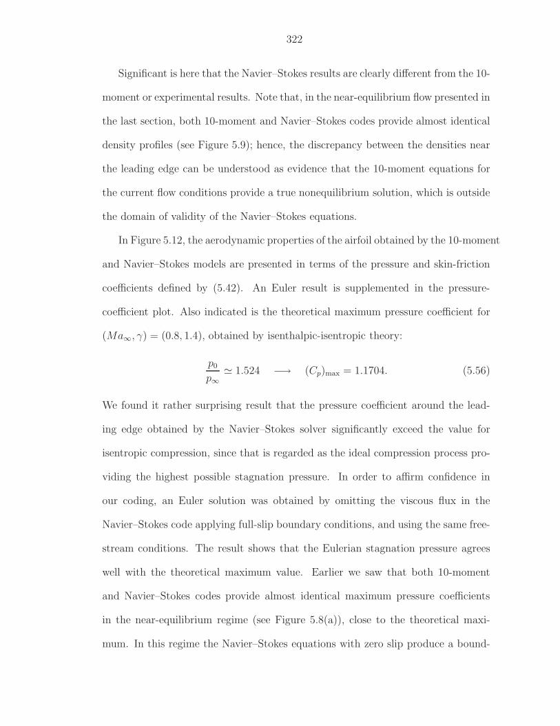
322
Significant is here that the Navier–Stokes results are clearly different from the 10-
moment or experimental results. Note that, in the near-equilibrium flow presented in
the last section, both 10-moment and Navier–Stokes codes provide almost identical
density profiles (see Figure 5.9); hence, the discrepancy between the densities near
the leading edge can be understood as evidence that the 10-moment equations for
the current flow conditions provide a true nonequilibrium solution, which is outside
the domain of validity of the Navier–Stokes equations.
In Figure 5.12, the aerodynamic properties of the airfoil obtained by the 10-moment
and Navier–Stokes models are presented in terms of the pressure and skin-friction
coefficients defined by (5.42). An Euler result is supplemented in the pressure-
coefficient plot. Also indicated is the theoretical maximum pressure coefficient for
(Ma∞, γ) = (0.8, 1.4), obtained by isenthalpic-isentropic theory:
p0
p∞≃ 1.524 −→ (Cp)max = 1.1704. (5.56)
We found it rather surprising result that the pressure coefficient around the lead-
ing edge obtained by the Navier–Stokes solver significantly exceed the value for
isentropic compression, since that is regarded as the ideal compression process pro-
viding the highest possible stagnation pressure. In order to affirm confidence in
our coding, an Euler solution was obtained by omitting the viscous flux in the
Navier–Stokes code applying full-slip boundary conditions, and using the same free-
stream conditions. The result shows that the Eulerian stagnation pressure agrees
well with the theoretical maximum value. Earlier we saw that both 10-moment
and Navier–Stokes codes provide almost identical maximum pressure coefficients
in the near-equilibrium regime (see Figure 5.8(a)), close to the theoretical maxi-
mum. In this regime the Navier–Stokes equations with zero slip produce a bound-
323
ary layer across which the pressure is practically constant, as in the Euler case. In
the continuum-transition regime, however, partial slip makes the pressure do work
at the bottom of the boundary layer, significantly changing its structure. We be-
lieve that this effect allows the unexpectedly high pressures to appear, but have not
further pursued this issue.
With the 10-moment model, stagnation pressures above the isenthalpic-isentropic
maximum value are not observed. It should be noted that in these equations, due
to the inclusion of a full pressure tensor, there is no single total enthalpy to be
defined, which the entropy only relates to the determinant of the pressure tensor;
see (5.2), (5.17). As a result, there is no procedure to determine a meaningful
maximum stagnation pressure.
We found that stagnation pressures computed with the IP and DSMC codes,
published elsewhere, significantly overshoot the isenthalpic-isentropic maximum
[FBC+01, SB02].
We conclude that the discrepancy between the solutions of the 10-moment and
the Navier–Stokes equations for the flow around a micro-airfoil can be attributed
to the significant nonequilibrium effect in the stagnation region.
The numerical results for the 10-moment equations obtained by two methods,
namely, HR2–Hancock and DG(1)–RK2, agree well except for the skin friction co-
efficient. This might be due to the convergence stall of the DG(1)–RK2 method;
it occurs after the residual drops three order of magnitude. Clearly, convergence-
acceleration methods need to be studies in combination with spatial DG discretiza-
tions.
The density profiles along the centerline of the airfoil are shown in Figure 5.13.
324
The isentropic relation provides the theoretical stagnation density,
ρ0
ρ∞≃ 1.351. (5.57)
As discussed previously, the maximum density predicted by the 10-moment equa-
tions is much lower than the values obtained by the Navier-Stokes equations with
slip velocity and by the Euler equations.
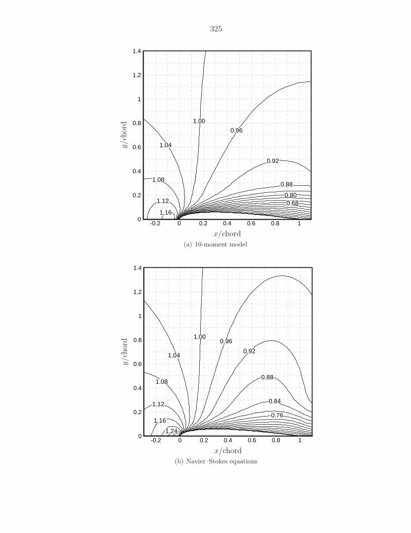
325
1.16
1.12
1.08
1.04
1.00
0.96
0.92
0.88
0.800.68
-0.2 0 0.2 0.4 0.6 0.8 10
0.2
0.4
0.6
0.8
1
1.2
1.4
x/chord
y/c
hor
d
(a) 10-moment model
1.08
1.04
1.12
1.24
1.16
1.000.96
0.92
0.88
0.84
0.76
-0.2 0 0.2 0.4 0.6 0.8 10
0.2
0.4
0.6
0.8
1
1.2
1.4
x/chord
y/c
hor
d
(b) Navier–Stokes equations
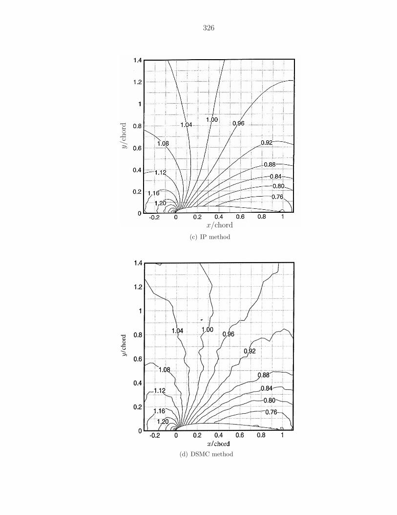
326
x/chord
y/c
hor
d
(c) IP method
(d) DSMC method
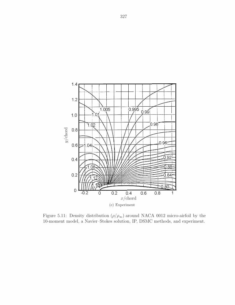
327
x/chord
y/c
hor
d
(e) Experiment
Figure 5.11: Density distribution (ρ/ρ∞) around NACA 0012 micro-airfoil by the10-moment model, a Navier–Stokes solution, IP, DSMC methods, and experiment.
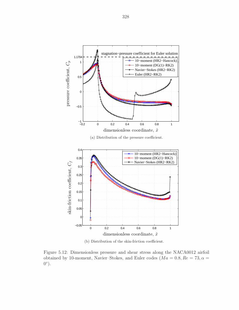
328
−0.2 0 0.2 0.4 0.6 0.8 1−1
−0.5
0
0.5
1
1.1704
stagnation−pressure coefficient for Euler solution
10−moment (HR2−Hancock)10−moment (DG(1)−RK2)Navier−Stokes (HR2−RK2)Euler (HR2−RK2)
dimensionless coordinate, x
pre
ssure
coeffi
cien
t,C
p
(a) Distribution of the pressure coefficient.
0 0.2 0.4 0.6 0.8 1−0.05
0
0.05
0.1
0.15
0.2
0.25
0.3
0.35
0.4
10−moment (HR2−Hancock)10−moment (DG(1)−RK2)Navier−Stokes (HR2−RK2)
dimensionless coordinate, x
skin
-fri
ctio
nco
effici
ent,
Cf
(b) Distribution of the skin-friction coefficient.
Figure 5.12: Dimensionless pressure and shear stress along the NACA0012 airfoilobtained by 10-moment, Navier–Stokes, and Euler codes (Ma = 0.8, Re = 73, α =0).
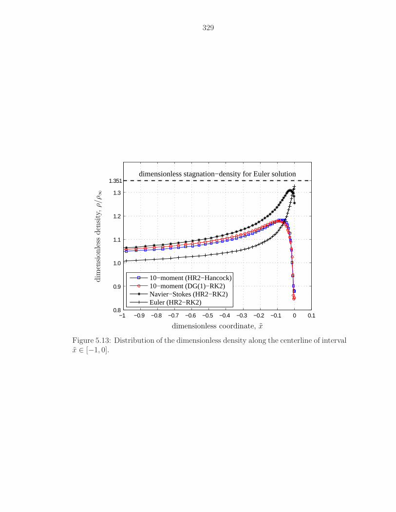
329
−1 −0.9 −0.8 −0.7 −0.6 −0.5 −0.4 −0.3 −0.2 −0.1 0 0.1 0.8
0.9
1.0
1.1
1.2
1.3
1.351
dimensionless stagnation−density for Euler solution
10−moment (HR2−Hancock)10−moment (DG(1)−RK2)Navier−Stokes (HR2−RK2)Euler (HR2−RK2)
dimensionless coordinate, x
dim
ensi
onle
ssden
sity
,ρ/ρ
∞
Figure 5.13: Distribution of the dimensionless density along the centerline of intervalx ∈ [−1, 0].
330
5.6 Avoiding Embedded Inviscid Shocks
The appearance of a discontinuity inside a steady viscous shock structure com-
puted with a hyperbolic-relaxation system indicates that the chosen relaxation term
is inadequate: it lacks information about the nonlinear characteristic fields of the
hyperbolic operator. To gain understanding, consider the 1-D hyperbolic-relaxation
system
ut + Aux = − s
τ, (5.58)
where the matrix A is the flux Jacobian. Assume there exists a traveling-wave
solution of the form
u(x, t) = u(z), z = x − ct, (5.59)
where c is the shock speed. Inserting this equation into the system yields the ODE
(−c I + A)u′ = − s
τ. (5.60)
Now express u′ and s in terms of the eigenvectors rk of A:
∑
k
(λk − c)C ′krk = −1
τ
∑
k
σkrk; (5.61)
here λk is an eigenvalue of A, C ′k is the corresponding characteristic variable, and
σk is the amplitude of the component along rk in the source vector.
Assume the shock is generated in the l-th field of characteristics; this means that
there is a point inside the shock structure where the difference between characteristic
speed and shock speed vanishes:
λl − c = 0. (5.62)
We may call this the sonic point. If in this point the amplitude σl does not vanish
simultaneously, C ′ can not remain finite, indicating the need to put a discontinuity
inside the viscous shock structure.
331
This is reminiscent of steady inviscid transonic flow in a converging-diverging
channel, which is ruled by the area-velocity relation:
(M2 − 1)u′ =A′
A. (5.63)
If the flow reaches the sonic point (M = 1) before arriving at the throat (A′ = 0),
u′ becomes infinite.
The following detailed example demonstrates how an inviscid embedded shock
is created, and, at the same time, how it can be avoided. Consider the hyperbolic-
relaxation system
ut + vx = 0, (5.64a)
vt + f 2u2ux = −v − 1
2u2
τ, f > 1; (5.64b)
its characteristic speeds are ±fu. For large times v approaches1
2u2, so the first
equation tends toward Burgers’ equation,
ut + uux = µuxx; (5.65)
the relation between µ and τ must still be determined. Note that the equilib-
rium equation has the characteristic speed u, which lies between the characteristic
speeds of the hyperbolic system, as required by the so-called subcharacteristic con-
dition [Liu87].
The traveling-wave solution satisfies
−cu′ + v′ = 0, (5.66a)
−cv′ + f 2u2u′ = −v − 1
2u2
τ. (5.66b)
332
Eliminating both v′ and v from the second equation by using the first equation leads
to the ODE
(−c2 + f 2u2)
2v0 − 2cu0 + c2 − (u − c)2du = −dz
2τ; (5.67)
without loss of generality we may choose the sonic point to lie at z = 0:
u0 = c. (5.68)
In a Burgers shock the profile is antisymmetric about this point.
In order to find a shock-like solution we must assume
2v0 − c2 = U2, (5.69)
where U is half the jump in u across the shock. The ODE now reads
(−c2 + f 2u2)
U2 − (u − c)2du = −dz
2τ, (5.70)
If the shock is slow enough, the shock structure will include the values u = ±c/f ,
causing the numerator on the LHS to vanish and u′ to become infinite. This will
lead to an inviscid shock between those values. In the special case of a steady shock
(c = 0), the profile is continuous, but it still has an infinite slope in the sonic point:
u ≈ 3
√
− 3U2
2f 2τz, z small. (5.71)
For systems relaxing to an equation more complicated than Burgers’ equation, the
profile is not antisymmetric around the sonic point, causing the inviscid jump to
appear even in a steady shock profile.
From (5.70) it is obvious that the LHS factor −c2 + f 2u2 is the culprit; we may
explore putting it also on the RHS, suitably normalized, i. e.,
−c2 + f 2u2
U2 − (u − c)2du = −−c2 + f 2u2
2U2τdz, (5.72)
333
or
du
U2 − (u − c)2= − dz
2U2τ, (5.73)
The solution of this ODE, with boundary conditions
u−∞ = c + U, u∞ = c − U, (5.74)
is
u = c − U tanh( z
2Uτ
), (5.75)
which is identical in form to the Burgers shock profile
u = c − U tanh
(Uz
2µ
). (5.76)
This shows how to choose the value of τ in order to relax to a viscosity coefficient
µ:
τ =µ
U2. (5.77)
Thus, the embedded inviscid shock has been completely removed.
In order to show that a time-marching scheme can find the proper asymptotic so-
lution of the hyperbolic-relaxation system, we used a standard second-order upwind-
biased finite-volume scheme with a two-stage time-integrator to find the steady
solution (c = 0) of the modified system
ut + vx = 0; (5.78a)
vt + f 2u2ux = −
(v − 1
2u2
)f 2u2
U2τ, (5.78b)
with f = 2.0, τ = 0.1, and boundary conditions
u±∞ = ±U, v±∞ = U, U = 1. (5.79)
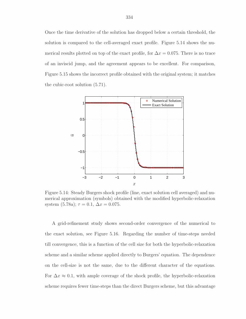
334
Once the time derivative of the solution has dropped below a certain threshold, the
solution is compared to the cell-averaged exact profile. Figure 5.14 shows the nu-
merical results plotted on top of the exact profile, for ∆x = 0.075. There is no trace
of an inviscid jump, and the agreement appears to be excellent. For comparison,
Figure 5.15 shows the incorrect profile obtained with the original system; it matches
the cubic-root solution (5.71).
−3 −2 −1 0 1 2 3
−1
−0.5
0
0.5
1
Numerical SolutionExact Solution
x
u
Figure 5.14: Steady Burgers shock profile (line, exact solution cell averaged) and nu-merical approximation (symbols) obtained with the modified hyperbolic-relaxationsystem (5.78a); τ = 0.1, ∆x = 0.075.
A grid-refinement study shows second-order convergence of the numerical to
the exact solution, see Figure 5.16. Regarding the number of time-steps needed
till convergence, this is a function of the cell size for both the hyperbolic-relaxation
scheme and a similar scheme applied directly to Burgers’ equation. The dependence
on the cell-size is not the same, due to the different character of the equations.
For ∆x ≈ 0.1, with ample coverage of the shock profile, the hyperbolic-relaxation
scheme requires fewer time-steps than the direct Burgers scheme, but this advantage
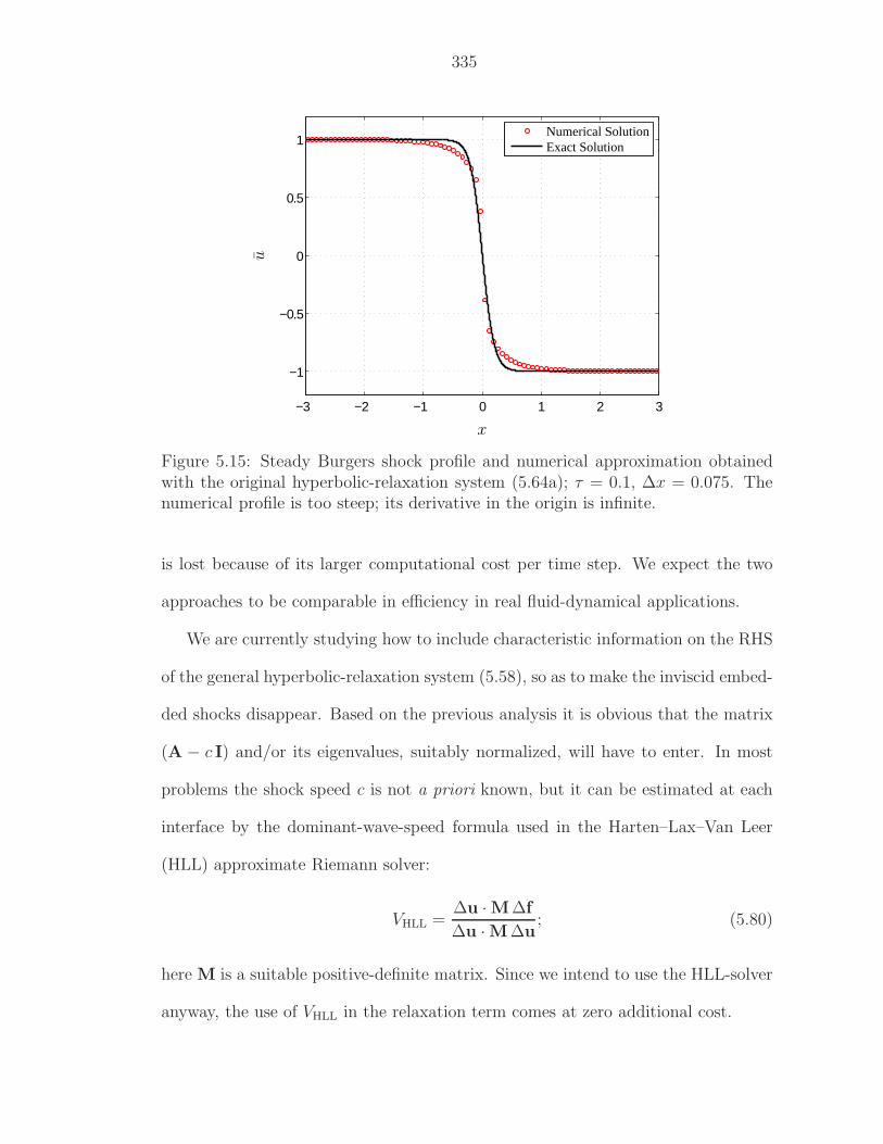
335
−3 −2 −1 0 1 2 3
−1
−0.5
0
0.5
1
Numerical SolutionExact Solution
x
u
Figure 5.15: Steady Burgers shock profile and numerical approximation obtainedwith the original hyperbolic-relaxation system (5.64a); τ = 0.1, ∆x = 0.075. Thenumerical profile is too steep; its derivative in the origin is infinite.
is lost because of its larger computational cost per time step. We expect the two
approaches to be comparable in efficiency in real fluid-dynamical applications.
We are currently studying how to include characteristic information on the RHS
of the general hyperbolic-relaxation system (5.58), so as to make the inviscid embed-
ded shocks disappear. Based on the previous analysis it is obvious that the matrix
(A − c I) and/or its eigenvalues, suitably normalized, will have to enter. In most
problems the shock speed c is not a priori known, but it can be estimated at each
interface by the dominant-wave-speed formula used in the Harten–Lax–Van Leer
(HLL) approximate Riemann solver:
VHLL =∆u · M∆f
∆u · M∆u; (5.80)
here M is a suitable positive-definite matrix. Since we intend to use the HLL-solver
anyway, the use of VHLL in the relaxation term comes at zero additional cost.
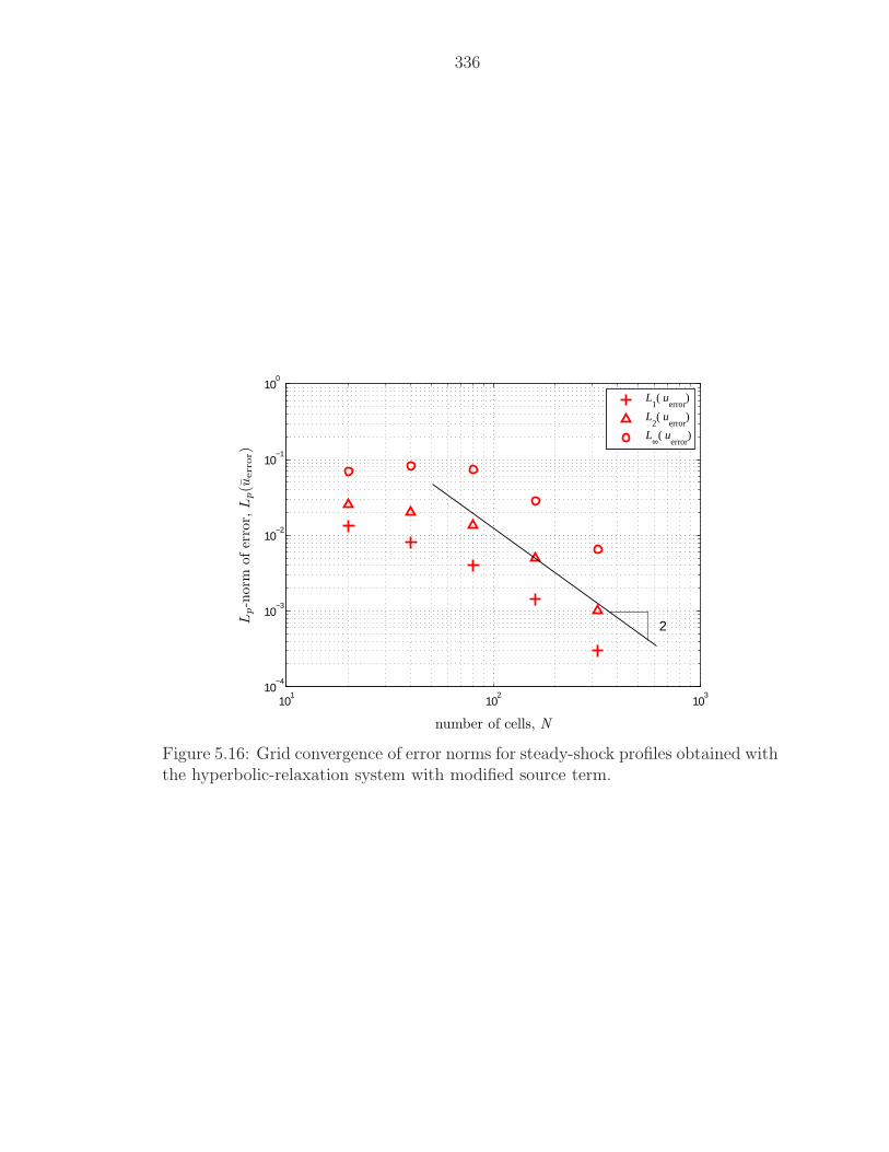
336
101
102
103
10−4
10−3
10−2
10−1
100
L
1( u
error)
L2( u
error)
L∞( u
error)
2
number of cells, N
Lp-n
orm
ofer
ror,L
p(u
err
or)
Figure 5.16: Grid convergence of error norms for steady-shock profiles obtained withthe hyperbolic-relaxation system with modified source term.
CHAPTER VI
CONCLUSIONS
6.1 Summary
In this thesis, a step towards a first-order PDE approach to computational fluid
dynamics is described. This approach is rather radical; the Navier–Stokes equa-
tions are no longer considered as target model equations to solve numerically. Our
motivation to move into such an unexplored area is due to the fact that currently
available numerical methodologies for advection-dominated compressible flows are
not necessarily efficient. Part of the reason is that these methods have trouble
remaining just second-order accurate on a distorted, unstructured grid. Further-
more, a numerical method intended to solve the Navier–Stokes equations can not
be applied to continuum-transition flows since the model equations themselves are
physically invalid in such a flow regime.
In order to advance beyond these issues that plague standard methods for the
compressible Navier–Stokes equations, namely, second-order Godunov-type finite-
volume methods, two approaches are taken: we adopt first-order PDEs as model
equations, and discretize them by a compact numerical method, i.e., the discontin-
uous Galerkin method.
The major contributions of this thesis are:
337
338
• Extension of Huynh’s original upwind moment method to systems of hyper-
bolic equations with stiff relaxation source terms, by utilizing Gauss–Radau
quadrature in time. We named the method the DG(1)–Hancock method
(Chapter II);
• Formulation of the fully discrete 2-D DG(1)–Hancock method on both quadri-
lateral and triangular elements (Chapter II);
• Detailed and comparative Fourier analysis of the DG(1)–Hancock method.
Dissipation/dispersion errors, order of accuracy, and stability are compared
to those of various fully and semi-discrete methods; it is shown that the
DG(1)–Hancock method is third-order accurate, with a less restrictive sta-
bility condition than semi-discrete methods. The high accuracy and efficiency
of the DG(1)–Hancock method are confirmed by numerical tests (Chapter III);
• The discovery that, for the DG(1)–Hancock method combined with the Ru-
sanov flux, the maximum Courant number based on the frozen-wave speed
depends on the value of the equilibrium-wave speed. In the 1-D case, its sta-
bility range varies from1
3to 1 as the equilibrium wave speed increases from
0 to 1. In the 2-D case, the maximum Courant number lies in the interval of
1
3to
2
3(Chapter III);
• Proof that the unconditional instability of DG(1) combined with the Lax–Friedrichs
flux is caused by the extraneous root. In general, the stability of the DG(1)
method combined with the upwind flux is restricted by high-frequency waves
(Chapter III);
• Linking the linear analysis of hyperbolic conservation laws to that of hyperbolic-
relaxation equations by defining a Courant number based on the frozen wave
339
speed, i.e., ν := 1∆t
∆x, instead of r
∆t
∆x. It is shown that an upwind method
for hyperbolic-relaxation equations in the near-equilibrium limit is equivalent
to directly discretizing the reduced equilibrium-equations with the Rusanov
flux (Chapter IV);
• Demonstration that the high efficiency of the DG(1)–Hancock method for
conservation laws is preserved when hyperbolic-relaxation equations are con-
sidered. The original Hancock method loses its efficiency in the stiff regime
since the effective flux is no longer upwind in this limit (Chapter IV);
• Explanation of the results of Lowrie and Morel [LM02], whose demonstration
of uniform second-order accuracy of DG(1) (independent of ǫ) turns out to
depend critically on their assumption that r = O(ǫ). In our scaling with
this limit, it is further shown that DG(1)–Hancock loses its superiority over
HR2–Hancock (Chapter IV);
• Numerical computation of the near-equilibrium solution (Navier–Stokes-like
limit) of a problem governed by the 1-D Euler equations with heat transfer
(Chapter IV);
• Numerical solutions of the 10-moment equations with the HR2–MOL, Han-
cock, and DG(1)–MOL methods. Computations of steady 1-D shock struc-
tures show the high accuracy of the DG(1) spatial discretization. A more
practical calculation, of an external flow around a micro-airfoil for which ex-
perimental results exist, serves as a benchmark, for comparison to results of
a Navier–Stokes solver and particle-based methods. An apparent advantage
of the 10-moment model over Navier–Stokes solvers is the treatment of the
slip velocity along the wall: it follows directly from the elements of the stress
340
tensor, which are state variables (Chapter V);
• Removal of the inviscid frozen shock (drawback of moment approach) in the
solution of hyperbolic-relaxation model system by a modification of the relax-
ation term (Chapter V).
6.2 Future Work
As it was mentioned previously, the first-order PDE approach is relatively new;
there are a great number of issues that need to be explored/solved in order to make
the approach competitive or even preferable to the conventional methodologies:
finite-volume Navier–Stokes solvers and DSMC. Here, we list a few topics for future
work:
• First and foremost, constructing robust and physically more realistic mod-
els beyond the 10-moment equations is necessary. The 10-moment equations
adopted in this thesis are the best known and most robust among sets of mo-
ment equations, but the model predicts frozen shocks (jumps) inside viscous
shock structures and does not permit heat transfer. Improvement in these
areas is critical for reliably computing high-speed flows. Higher-moment sys-
tems have been developed and are being numerically studied, but they are not
quite robust [Bro96];
• The efficiency and accuracy of the DG(1)–Hancock method on a distorted,
unstructured grid needs to be investigated numerically, and possibly com-
plemented with a Fourier analysis on right triangles; our current results are
restricted to either rectangular or quadrilateral grids;
• Extending the DG(1)–Hancock method, currently third-order accurate for hy-
341
perbolic conservation laws, to higher-order accuracy or possibly arbitrary or-
der is a challenge. In order to achieve this goal, a genuine space-time dis-
cretization is necessary; the resulting method is likely to be implicit. Yet,
first-order PDE’s often lead to a point-implicit method, whereas the Navier–
Stokes solvers usually can not avoid global data-dependence;
• Particularly for DG methods, two issues are still remaining: the necessity of
more sophisticated limiters that will allow higher than second-order accuracy
of multi-dimensional solutions, and reduction of the computational run-time.
Resolving these two issues will be a condition for attracting CFD practitioners;
• The method of moments is used to derive moment equations from the Boltz-
mann equation. Similarly, the method of moments (weak formulation) is
adopted to derive a discontinuous Galerkin method for given PDEs. A link
between these two procedures, one at the PDE level and the other at the
discrete level, might exist, and they may be treated uniformly;
• The treatment of slip velocity on a curved wall is vague, especially for Navier–Stokes
solvers. Rigorous analytical and numerical investigations are necessary for
both Navier–Stokes and moment approaches;
• Development of the ultimate scheme/flux function which would produce the
upwind method in the equilibrium limit is still worth pursuing.

APPENDICES
342
343
APPENDIX A
Implementation of Coordinate Transformations
In Chapter II, the multidimensional DG(1)–Hancock method was introduced. The
method is formulated such that both quadrilateral and triangular elements can be
used. In the final update formulas (2.88) on page 78, three coordinate-dependent
terms appear: mass matrix, |Aj|, Kj1, Kj2, Kj3, length of an edge in the surface
integral, and volume integral of the flux
∫∫
Kj
(·) dx. While computing an edge length
is trivial, the mass matrix and the quadrature for the volume integral depend on the
shape of the element. For implementation purposes, specific formulations of these
geometrically dependent quantities and the volume integral in the local coordinates
are presented in this appendix. The implementation of more complex elements,
e.g., curved elements, three-dimensional elements, can be found in [ZTZ05, KS05,
Hug00, Li06].
A.1 Quadrilateral Elements
Figure A.1 shows the schematic of a coordinate transformation from the quadri-
lateral global element Kj to the square local element Kj = [−1, 1] × [−1, 1]. Any
coordinates x = (x, y) in Kj are parameterized by bilinear functions of ξ = (ξ, η)
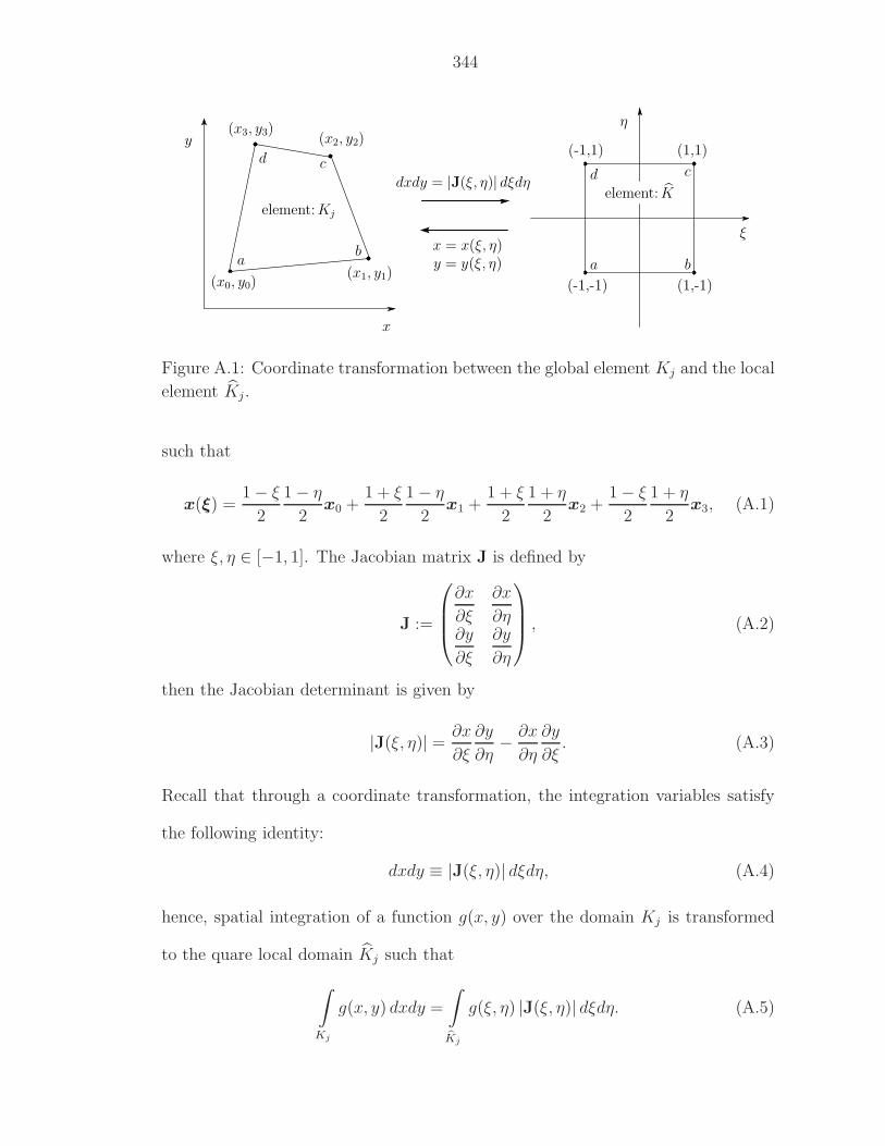
344
x
(x0, y0)(x1, y1)
(x2, y2)(x3, y3)
y
element:Kj
(-1,-1) (1,-1)
(1,1)(-1,1)
ξ
η
element: K
x = x(ξ, η)y = y(ξ, η)
dxdy = |J(ξ, η)| dξdη
ab
cd
a b
cd
Figure A.1: Coordinate transformation between the global element Kj and the local
element Kj .
such that
x(ξ) =1 − ξ
2
1 − η
2x0 +
1 + ξ
2
1 − η
2x1 +
1 + ξ
2
1 + η
2x2 +
1 − ξ
2
1 + η
2x3, (A.1)
where ξ, η ∈ [−1, 1]. The Jacobian matrix J is defined by
J :=
∂x
∂ξ
∂x
∂η∂y
∂ξ
∂y
∂η
, (A.2)
then the Jacobian determinant is given by
|J(ξ, η)| = ∂x
∂ξ
∂y
∂η− ∂x
∂η
∂y
∂ξ. (A.3)
Recall that through a coordinate transformation, the integration variables satisfy
the following identity:
dxdy ≡ |J(ξ, η)| dξdη, (A.4)
hence, spatial integration of a function g(x, y) over the domain Kj is transformed
to the quare local domain Kj such that
∫
Kj
g(x, y) dxdy =
∫
Kj
g(ξ, η) |J(ξ, η)| dξdη. (A.5)
345
By applying the above transformation, components of the mass matrix of a quadri-
lateral element in the global coordinates are analytically evaluated by the coordi-
nates of its nodes:
|Aj| :=
∫∫
Kj
dxdy =
∫∫
K
|J(ξ, η)| dξdη
=1
2[(x0 − x2)(y1 − y3) − (x1 − x3)(y0 − y2)] , (A.6)
∫∫
Kj
x dxdy =
∫∫
K
x(ξ, η)|J(ξ, η)| dξdη
=1
6
[(x0 − x2)(x1y1 − x3y3) − (x1 − x3)(x0y0 − x2y2)
+ (x20 − x2
2)(y1 − y3) − (x21 − x2
3)(y0 − y2)],
(A.7)
∫∫
Kj
y dxdy =
∫∫
K
y(ξ, η)|J(ξ, η)| dξdη
= −1
6
[(y0 − y2)(x1y1 − x3y3) − (y1 − y3)(x0y0 − x2y2)
+ (y20 − y2
2)(x1 − x3) − (y21 − y2
3)(x0 − x2)],
(A.8)
∫∫
Kj
x2 dxdy =1
12
[(x3
0 − x32)(y1 − y3) − (x3
1 − x33)(y0 − y3)
+ (x20 − x2
2)(x1y1 − x3y3) − (x21 − x2
3)(x0y0 − x2y2)
+ (x0 − x2)(x21y1 − x2
3y3) − (x1 − x3)(x20y0 − x2
2y2)], (A.9)
∫∫
Kj
y2 dxdy = − 1
12
[(y3
0 − y32)(x1 − x3) − (y3
1 − y33)(x0 − x3)
+ (y20 − y2
2)(x1y1 − x3y3) − (y21 − y2
3)(x0y0 − x2y2)
+ (y0 − y2)(x1y21 − x3y
23) − (y1 − y3)(x0y
20 − x2y
22)], (A.10)
346
∫∫
Kj
xy dxdy =1
12
[(x0 − x2)(x1y
21 − x3y
23) − (x1 − x3)(x0y
20 − x2y
22)
− (y0 − y2)(x21y1 − x2
3y3) + (y1 − y3)(x20y0 − x2
2y2)
+1
2
((x2
0 − x22)(y
21 − y2
3) − (x21 − x2
3)(y20 − y2
2))]
. (A.11)
The above geometric quantities (metrics) are evaluated analytically since the coor-
dinate transformation is expressed in bilinear form (A.1).
Conversely, a quadrature is necessary to evaluate the nonlinear flux tensor
f(u(x)). As described in its derivation, the four-point Gauss quadrature (see Fig-
ure 2.8 on page 74) is employed to approximate the spatial integration:
∫
Kj
f(u(x)) dx =
∫
K
f(u(ξ))|J(ξ)| dξ
≈3∑
i=0
wi|J(ξi)| f(u(ξi)), (A.12)
where the weights are wi =1
4, i = 0, . . . , 3, and the Gauss points where the flux
tensor is evaluated are
ξ0 =
(− 1√
3,− 1√
3
), ξ1 =
(1√3,− 1√
3
), (A.13a)
ξ2 =
(1√3,
1√3
), ξ3 =
(− 1√
3,
1√3
). (A.13b)
The solution at the Gauss point u(ξi) is computed by its solution representa-
tion (2.58a) on page 61 together with the coordinate transformation from ξ to
x given by (A.1).
A.2 Triangular Elements
At first, it is worthwhile to mention that a triangular element can be subdivided
into three quadrilateral elements [Hug00, p. 165]. See Figure A.2.
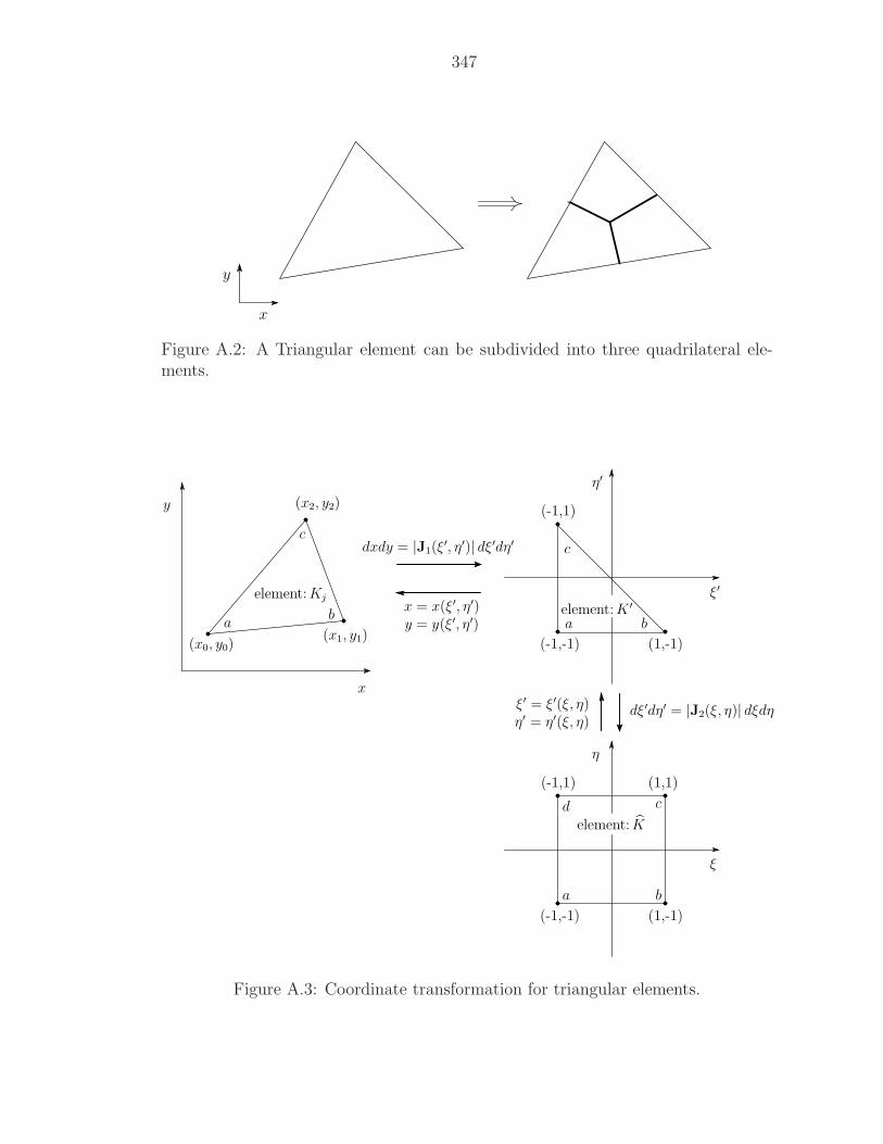
347
x
y
Figure A.2: A Triangular element can be subdivided into three quadrilateral ele-ments.
x
(x0, y0)(x1, y1)
(x2, y2)y
element:Kj
(-1,-1) (1,-1)
(1,1)(-1,1)
ξ
η
element: K
a b
cd
x = x(ξ′, η′)y = y(ξ′, η′)
dxdy = |J1(ξ′, η′)| dξ′dη′
ab
cc
baelement:K ′
η′
ξ′
(-1,1)
(1,-1)(-1,-1)
dξ′dη′ = |J2(ξ, η)| dξdηξ′ = ξ′(ξ, η)η′ = η′(ξ, η)
Figure A.3: Coordinate transformation for triangular elements.
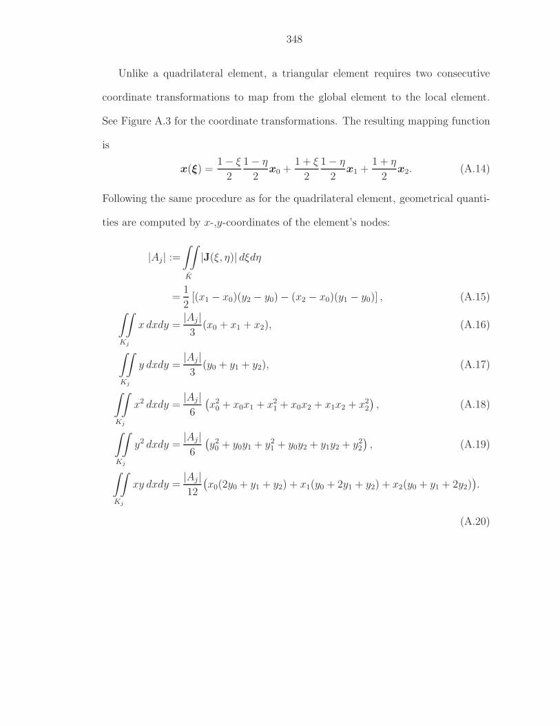
348
Unlike a quadrilateral element, a triangular element requires two consecutive
coordinate transformations to map from the global element to the local element.
See Figure A.3 for the coordinate transformations. The resulting mapping function
is
x(ξ) =1 − ξ
2
1 − η
2x0 +
1 + ξ
2
1 − η
2x1 +
1 + η
2x2. (A.14)
Following the same procedure as for the quadrilateral element, geometrical quanti-
ties are computed by x-,y-coordinates of the element’s nodes:
|Aj| :=
∫∫
K
|J(ξ, η)| dξdη
=1
2[(x1 − x0)(y2 − y0) − (x2 − x0)(y1 − y0)] , (A.15)
∫∫
Kj
x dxdy =|Aj|3
(x0 + x1 + x2), (A.16)
∫∫
Kj
y dxdy =|Aj|3
(y0 + y1 + y2), (A.17)
∫∫
Kj
x2 dxdy =|Aj|6
(x2
0 + x0x1 + x21 + x0x2 + x1x2 + x2
2
), (A.18)
∫∫
Kj
y2 dxdy =|Aj|6
(y2
0 + y0y1 + y21 + y0y2 + y1y2 + y2
2
), (A.19)
∫∫
Kj
xy dxdy =|Aj|12
(x0(2y0 + y1 + y2) + x1(y0 + 2y1 + y2) + x2(y0 + y1 + 2y2)
).
(A.20)
349
APPENDIX B
Fourier Analysis of High-Order Methods
The Fourier analysis of three high-order methods is conducted as a continuation of
previous analyses shown in Chapter III. The difference operator and local truncation
error of each method are presented in a concise manner.
B.1 HR3–RK3 method
The third-order high-resolution Godunov method (HR3–MOL) utilizes quadratic
reconstructed values as input for the flux function. The input values are given by
uj+1/2,L(t) = uj +∆x
2
(uj+1 − uj−1
2∆x
)+
∆x2
12
(uj+1 − 2uj + uj−1
∆x2
), (B.1a)
uj+1/2,R(t) = uj+1 −∆x
2
(uj+2 − uj
2∆x
)+
∆x2
12
(uj+2 − 2uj+1 + uj
∆x2
). (B.1b)
After inserting the cell interface fluxes into the original semi-discrete form, the
spatial difference operator becomes
NHR3 = − 1
12∆x
[(q − r)(δ+)2 − 2(q − 3r)δ+ + 2(q + 3r)δ− + (q + r)(δ−)2
], (B.2)
or, for a Fourier mode,
NHR3 = − 1
12∆x
[(q − r)e2iβ − 4(q − 2r)eiβ + 6q − 4(q + 2r)e−iβ + (q + r)e−2iβ
].
(B.3)
350
The spatial discretization in the low-frequency limit has the following discretization
error:
λHR3 − λexact = − q
12∆x3 k4 + O
(k5), (B.4)
thus, the HR3 method is third-order accurate in space. Applying the RK3 method
as the time integrator, the local truncation error becomes
LTEHR3RK3 = − r
12
(q
r∆x3 +
1
2r3 ∆t3
)k4 + O
(k5). (B.5)
Thus, the HR3–RK3 method is third-order accurate in space and time.
B.2 DG(2)–RK3 method
The DG(2)–MOL introduces an extra update equation for ∆2uj :
∂∆2uj(t)
∂t= − 1
∆x60(fj+1/2(t) − fj−1/2(t) − r∆uj(t)
). (B.6)
The above update equation together with two update equations for uj(t) and ∆uj(t)
given by (3.97) on page 119 are solved simultaneously. Similar to HR3–MOL, the
input values for the flux function are obtained by the quadratic solution represen-
tation:
uj+1/2,L(t) = uj +1
2∆uj +
1
12∆2uj, (B.7a)
uj+1/2,R(t) = uj+1 −1
2∆uj+1 +
1
12∆2uj+1. (B.7b)
After inserting the cell interface fluxes into the original semi-discrete form, the
spatial difference operator becomes
NDG(2) = A+D+ + C + A
−D−, (B.8)
351
where
A+ =
q − r
2∆x
1 −1
2
1
12
6 −31
2
60 −30 5
, A− =
q + r
2∆x
−1 −1
2− 1
12
6 31
2
−60 −30 −5
, (B.9a)
C =1
∆x
0 0 0
0 −6q
r−1
0 60 0
, D± = δ±I, (B.9b)
or, for a Fourier mode,
MDG(2) = A+eiβI + C
′ − A−e−iβI, (B.10)
where
C′ = − r
∆x
q
r
1
2
q
12r
−63q
r
1
260q
r−30
5q
r
. (B.11)
The asymptotic eigenvalues in the low-frequency limit are obtained by solving the
characteristic equation of NDG(2). Here, we only present the result with the upwind
flux q = r:
λ(1)DG(2) − λexact = − r
7200∆x5 k6 + O
(k7), (B.12)
λ(2),(3)DG(2) − λexact = − r
∆x(3 ± i
√51) + O(k) . (B.13)
The above equations show that the accurate eigenvalue of the DG(2) spatial dis-
cretization is fifth-order in space. Also, similar to the DG(1) method, inaccurate
eigenvalues damp quickly since the real part of the leading error, − 3r
∆x, is negative
for both λ(2)DG(2) and λ
(3)DG(2). Applying the RK3 method for the time integrator, the
local truncation error becomes
LTEDG(2)RK3 = − r
24(rν)3 ∆x3 k4 + O
(k5), (B.14)
352
thus, the DG(2)–RK3 method is third-order in space and time. Note that the above
error is introduced purely by the time integration method since the DG(2) spatial
discretization is fifth-order accurate. Hence, it is natural to apply the fifth-order
time integration method, RK5; then the local truncation error becomes
LTEDG(2)RK5 = − r
7200
[1 + 50(rν)5
]∆x5 k6 + O
(k7), (B.15)
and the method becomes fifth-order accurate. This linear analysis suggests that
when the DG discretization adopts the solution representation of a polynomial of
degree k, then the corresponding time integrator is recommended to have the order
of accuracy 2k + 1. Another benefit of using higher-order Runge–Kutta method
is enlarging the stability domain. However, increasing the number of stages of a
time-integration method results in greater computational expense due to the Rie-
mann problem to be solved at each stage.
B.3 DG(2)–ADER method
The DG(2)–ADER method is obtained by approximating the volume integral of
the flux as follows:
1
∆t
∫
T n
f(uj) ≈ r
(un
j − 1
2r∆t
∆un
j
∆x+
1
6(r∆t)2
∆2un
j
∆x2
), (B.16)
∆x
∆t
∫
T n
∂f(uj)
∂x≈ r
(∆u
n
j − 1
2r∆t
∆2un
j
∆x
). (B.17)
After inserting the difference forms, the spatial difference operator of the DG(2)–ADER
method has the following form:
MDG(2)ADER = A+D+ + C + A
−D−, (B.18)
353
where
A+ =
q − r
2∆x
1 −1
2(1 + rν)
1
12(1 + rν)(1 + 2rν)
6 −3(1 + rν)1
2(1 + rν)(1 + 2rν)
60 −30(1 + rν) 5(1 + rν)(1 + 2rν)
, (B.19a)
A− =
q + r
2∆x
−1 −1
2(1 − rν) − 1
12(1 − rν)(1 − 2rν)
6 3(1 − rν)1
2(1 − rν)(1 − 2rν)
−60 −30(1 − rν) −5(1 − rν)(1 − 2rν)
, (B.19b)
C =1
∆x
0 0 0
0 −6q
r−(1 − 3qν)
0 60 −30rν
, D± = δ±I, (B.19c)
or, for a Fourier mode,
MDG(2)ADER = A+eiβI + C
′ − A−e−iβI, (B.20)
where
C′ = − r
∆x
q
r
1
2(1 − qν)
1
12
(q
r− 3rν +
2q
r(rν)2
)
−6 3(q
r+ rν
) 1
2
(1 − 3qν − 2(rν)2
)
60q
r−30(1 + qν) 5
(q
r+ 3rν +
2q
r(rν)2
)
. (B.21)
The overall accuracy is derived from the eigenvalues of the amplification matrix of a
fully discrete form, GDG(2)ADER = I+∆tMDG(2)ADER. Due to the complexity of the
derivation, we only present the case of the upwind flux q = r. The local truncation
error of the accurate mode becomes
LTE(1),upwindDG(2)ADER = − r
120rν(1 − rν) ∆x3 k4 + O
(k5). (B.22)
Thus, DG(2)–ADER method is third-order in space and time.
354
APPENDIX C
Asymptotic Expansion of Dimensionless GHHE
C.1 One-Dimensional Systems
Let us consider the dimensionless 1-D GHHE with frozen-wave time-scaling;
removing the (·) symbol in (4.16) on page 213 for simplicity yields
∂tu + ∂xv = 0, (C.1a)
∂tv + ∂xu = −1
ǫ(v − ru), (C.1b)
where |r| ≤ 1 is fixed, and ǫ > 0 can vary. The dimensionless time t and conserved
variable u are set to O(1). Compared to the dimensional form (4.1) on page 208, the
above system shows frozen wave speeds aF = ±1, the equilibrium speed aE = r, and
the relaxation time τ = ǫ. Here, we present the derivation of the reduced equation
in the near-equilibrium limit. The derivation is based on the assumption that, in
the near-equilibrium, the state vector u, v can be expanded in terms of a small
parameter, the relaxation time ǫ, such that
u(x, t) = u0 + ǫu1 + ǫ2u2 + ǫ3u3 + O(ǫ4), (C.2a)
v(x, t) = v0 + ǫv1 + ǫ2v2 + ǫ3v3 + O(ǫ4). (C.2b)
355
These expansions are called Chapman–Enskog expansions. The above equations are
inserted into (C.1), and terms of the same order of ǫ are gathered. Since ui, vi, i =
0, 1, . . ., are not functions of ǫ, the coefficient of any power of ǫ has to be zero. After
some algebra, we have
v0 = ru0, (C.3a)
v1 = ru1 − (1 − r2)∂xu0, (C.3b)
v2 = ru2 − (1 − r2)∂xu1 − 2r(1 − r2)∂xxu0, (C.3c)
v3 = ru3 − (1 − r2)∂xu2 − 2r(1 − r2)∂xxu1 − (1 − r2)(5r2 − 1)∂xxxu0, (C.3d)
thus, the flux v can be expressed in the conservative variable u such that
v = ru− ǫ (1−r2)∂xu− ǫ2 2r(1−r2)∂xxu− ǫ3 (1−r2)(5r2−1)∂xxxu+O(ǫ4). (C.4)
Inserting the above equation into (C.1a) provides the reduced form of the dimen-
sionless GHHE:
∂tu+ r∂xu = ǫ (1− r2)∂xxu+ ǫ2 2r(1− r2)∂xxxu+ ǫ3 (1− r2)(5r2−1)∂xxxxu+O(ǫ4).
(C.5)
Note that this reduced form is valid only when ǫ ≪ O(1) (near-equilibrium limit).
As we can see, the equation has the form of an advection-diffusion equation with
higher-order dissipation and dispersion terms; the equilibrium advection wave speed
is r, and the leading dissipation coefficient is ǫ (1 − r2). Truncating the above
equation at O(ǫ2) leads to the advection-diffusion equation:
∂tu + r∂xu = ǫ (1 − r2)∂xxu. (C.6)
356
C.2 Two-Dimensional Systems
Following the same procedure as in the 1-D case, the coefficients in the asymp-
totic expansions of v and w are given by
v0 = ru0, v1 = ru1 − (1 − r2)∂xu0, (C.7)
w0 = su0, w1= su1 − (1 − s2)∂yu0. (C.8)
Thus, the fluxes can be expressed in the conservative variable u such that
v = ru − ǫ(1 − r2)∂xu + O(ǫ2), (C.9)
w = su − ǫ(1 − s2)∂yu + O(ǫ2). (C.10)
Inserting the above equations into the original PDE for u leads to the reduced form
of the 2-D GHHE in the near-equilibrium limit (ǫ ≪ 1):
∂tu + r∂xu + s∂yu = ǫ[(1 − r2)∂xxu + (1 − s2)∂yy
]+ O
(ǫ2). (C.11)
357
APPENDIX D
Jin–Levermore’s Semi-Discrete High-Resolution
Godunov Method
Jin and Levermore already realized that the upwind flux in a Godunov method
for the original hyperbolic-relaxation equations does not retain the upwind prop-
erty in the near-equilibrium limit [JL96]. In other words, the discretization in the
near-equilibrium limit is equivalent to discretizing the advection-diffusion equation
directly with a somewhat more dissipative flux function. Later, it was shown that
the corresponding flux is the first HLL1 flux function [HSvL05].
To remedy the excessive numerical dissipation in the near-equilibrium limit due
to a non-upwind flux, Jin and Levermore came up with the idea to interlace two
flux functions: one is upwind for the frozen system, and the other is upwind for the
equilibrium system. The simplest way is by a linear combination: introduce the
parameter a ∈ [0, 1] such that
f = affrozen + (1 − a)fequilibrium, (D.1)
where
a ∼ ǫ
∆x. (D.2)
358
They chose the parameter a such that in the frozen limit (ǫ ≫ 1), it approaches
unity, so that the original upwind flux ffrozen is applied. Conversely, in the near-
equilibrium limit (ǫ ≪ 1), a small a turns off the frozen flux, and the equilibrium
flux fequilibrium, which is upwind for the reduced equation, becomes dominant. Note
that this modification is only applied to the flux of the conserved quantity, i.e., to
the first equation of the GHHE.
Here, the method is applied to the 1-D GHHE, and a Fourier analysis is con-
ducted. The semi-discrete form is identical to the HR2–MOL method,
∂uj(t)
∂t= − 1
∆x
(fj+1/2 − fj−1/2
)+
1
ǫs (uj) , (D.3)
yet, the interface flux is computed by the following hybrid flux:
fj+1/2 =
vj+1/2
uj+1/2
=
af1,frozen + (1 − a)
[fequi − ǫ(1 − r2)
uj+1 − uj
∆x
]
f2,frozen
. (D.4)
The frozen flux is obtained by the system
u
v
t
+
0 1
1 0
u
v
x
= 0, −→
f1, frozen
f2, frozen
= A+uL + A−uR, (D.5)
and the equilibrium flux by
ut + rux = 0 −→ fj+1/2,equi = ruj+1/2,L. (D.6)
Following the usual procedure for a Fourier analysis, the truncation errors in the
low-frequency limit is given by
λ(1)HR2–JL − λGHHE
exact = − ir
12∆x2k3 −
[1
8
(a + (1 − a)r
)∆x3 +
ǫ(1 − r2)
12(3a − 1)∆x2
]k4
+ O(ǫ2k3, ǫ3k4, k5
),
(D.7a)
λ(2)HR2–JL − λGHHE
exact = −1
ǫ+ ir(1 + a)k + O
(k2). (D.7b)
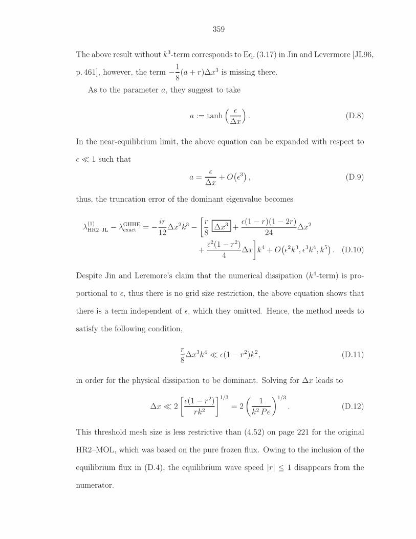
359
The above result without k3-term corresponds to Eq. (3.17) in Jin and Levermore [JL96,
p. 461], however, the term −1
8(a + r)∆x3 is missing there.
As to the parameter a, they suggest to take
a := tanh( ǫ
∆x
). (D.8)
In the near-equilibrium limit, the above equation can be expanded with respect to
ǫ ≪ 1 such that
a =ǫ
∆x+ O
(ǫ3), (D.9)
thus, the truncation error of the dominant eigenvalue becomes
λ(1)HR2–JL − λGHHE
exact = − ir
12∆x2k3 −
[r
8∆x3 +
ǫ(1 − r)(1 − 2r)
24∆x2
+ǫ2(1 − r2)
4∆x
]k4 + O
(ǫ2k3, ǫ3k4, k5
). (D.10)
Despite Jin and Leremore’s claim that the numerical dissipation (k4-term) is pro-
portional to ǫ, thus there is no grid size restriction, the above equation shows that
there is a term independent of ǫ, which they omitted. Hence, the method needs to
satisfy the following condition,
r
8∆x3k4 ≪ ǫ(1 − r2)k2, (D.11)
in order for the physical dissipation to be dominant. Solving for ∆x leads to
∆x ≪ 2
[ǫ(1 − r2)
rk2
]1/3
= 2
(1
k2 Pe
)1/3
. (D.12)
This threshold mesh size is less restrictive than (4.52) on page 221 for the original
HR2–MOL, which was based on the pure frozen flux. Owing to the inclusion of the
equilibrium flux in (D.4), the equilibrium wave speed |r| ≤ 1 disappears from the
numerator.
360
APPENDIX E
Dispersion Analysis for the 2-D GHHE
Following the dispersion analysis of Hittinger for the 1-D GHHE model system [Hit00,
pp. 35–47], we assume a harmonic solution,
u(x, y, t) = ℜv(t) exp(−i(kxx + kyy)
), (E.1)
where (kx, ky) are wave numbers in (x, y). Inserting this into (4.107) on page 237
leads to an ordinary differential equation in terms of v(t),
dv(t)
dt= [i(kxA + kyB) + Q]v(t). (E.2)
The solution of this is
v(t) = exp [it(kxA + kyB − iQ)] u0, (E.3)
where u0 ∈ C3 is a constant vector. The characteristic polynomial of the exponent
is
det [kxA + kyB − iQ − ωI] = 0, (E.4a)
↓
(i − ω)(ω2 − |k|2 − i [ω + (rkx + sky)]
)= 0, (E.4b)
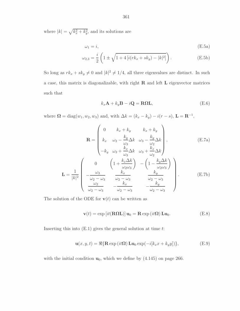
361
where |k| =√
k2x + k2
y, and its solutions are
ω1 = i, (E.5a)
ω2,3 =i
2
(1 ±
√1 + 4 [i(rkx + sky) − |k|2]
). (E.5b)
So long as rkx + sky 6= 0 and |k|2 6= 1/4, all three eigenvalues are distinct. In such
a case, this matrix is diagonalizable, with right R and left L eigenvector matrices
such that
kxA + kyB − iQ = RΩL, (E.6)
where Ω = diag(w1, w2, w3) and, with ∆k = (kx − ky) − i(r − s), L = R−1,
R =
0 kx + ky kx + ky
kx ω2 −ky
ω3∆k ω3 −
ky
ω2∆k
−ky ω2 +kx
ω3∆k ω3 +
kx
ω2∆k
, (E.7a)
L =1
|k|2
0
(1 +
kx∆k
ω2ω3
)−(
1 − ky∆k
ω2ω3
)
− ω3
ω2 − ω3
kx
ω2 − ω3
ky
ω2 − ω3
ω2
ω2 − ω3− kx
ω2 − ω3− ky
ω2 − ω3
. (E.7b)
The solution of the ODE for v(t) can be written as
v(t) = exp [it(RΩL)]u0 = R exp (itΩ)Lu0. (E.8)
Inserting this into (E.1) gives the general solution at time t:
u(x, y, t) = ℜR exp (itΩ)Lu0 exp(−i[kxx + kyy]), (E.9)
with the initial condition u0, which we define by (4.145) on page 266.

BIBLIOGRAPHY
362
363
BIBLIOGRAPHY
[AG87] S. Allmaras and M. Giles. A second order flux split scheme for theunsteady 2-D Euler equations on arbitrary meshes. In 8th AIAAComputational Fluid Dynamics Conference, Honolulu, Hawai; USA,June 9–11, 1987. AIAA Paper 1987-1119.
[AH99] R. K. Agarwal and D. W. Halt. A compact high-order unstructuredgrids method for the solution of Euler equations. International Jour-nal for Numerical Methods in Fluids, 31(1):121–147, 1999.
[All89] S. R. Allmaras. A Coupled Euler/Navier–Stokes Algorithm for 2-DUnsteady Transonic Shock/Boundary-Layer Interaction. PhD thesis,Massachusetts Institute of Technology, 1989.
[AM07] R. Abgrall and F. Marpeau. Residual distribution schemes onquadrilateral meshes. Journal of Scientific Computing, 30(1):131–175, 2007.
[AR97] M. Arora and P. L. Roe. Characteristic-based numerical algorithmsfor stiff hyperbolic relaxation systems. In P. Kutler, J. Flores, and J.-J. Chattot, editors, Fifteenth International Conference on NumericalMethods in Fluid Dynamics: Proceedings of the Conference Held inMonterey, CA, USA, 24-28 June 1996, Lecture Notes in Physics,Volume 490. Springer-Verlag, Berlin, 1997.
[AR98] M. Arora and P. L. Roe. Issues and strategies for hyperbolic prob-lems with stiff source terms. In V. Venkatakrishnan, M. D. Salas,and S. R. Chakravarthy, editors, Barriers and Challenges in Com-putational Fluid Dynamics, ICASE/LaRC Interdisciplinary Series inScience and Engineering, pages 139–154. Kluwer Academic Publish-ers, Dordrecht, 1998.
[Ari01] V. V. Aristov. Direct Methods for Solving the Boltzmann Equationand Study of Nonequilibrium Flows. Fluid Mechanics and Its Appli-cations, Volume 60. Kluwer Academic Publishers, Dordrecht, 2001.
364
[ARL87] J. Allegre, M. Raffin, and J. C. Lengrand. Experimental flowfieldsaround NACA 0012 airfoils located in subsonic and supersonic rar-efied air streams. In M. O. Bristeau, R. Glowinski, J. Periaux, andH. Viviand, editors, Numerical Simulation of Compressible Navier–Stokes Flows: A GAMM-Workshop, Notes on Numerical Fluid Me-chanics, Volume 18, pages 59–68. Friedrick Vieweg & Sohn, Braun-schweig, 1987.
[ARS97] U. M. Ascher, S. J. Ruuth, and R. J. Spiteri. Implicit-explicit Runge–Kutta methods for time-dependent partial differential equations. Ap-plied Numerical Mathematics, 25(2-3):151–167, 1997.
[ARW95] U. M. Ascher, S. J. Ruuth, and B. T. R. Wetton. Implicit-explicitmethods for time-dependent partial differential equations. SIAMJournal on Numerical Analysis, 32(3):797–823, 1995.
[AS96] H. L. Atkins and C.-W. Shu. Quadrature-free implementation ofthe discontinuous Galerkin method for hyperbolic equations. In 2ndAIAA and CEAS Aeroacoustics Conference, State College, Pennsyl-vania; USA, May 6–8, 1996. AIAA Paper 1996-1683.
[AS98] H. L. Atkins and C.-W. Shu. Quadrature-free implementation of dis-continuous Galerkin method for hyperbolic equations. AIAA Jour-nal, 36(5):775–782, 1998.
[AYB01] R. K. Agarwal, K.-Y. Yun, and R. Balakrishnan. Beyond Navier–Stokes: Burnett equations for flows in the continuum-transitionregime. Physics of Fluids, 13(10):3061–3085, 2001.
[Bal04] R. Balakrishnan. An approach to entropy consistency in second-order hydrodynamic equations. Journal of Fluid Mechanics,503:201–245, 2004.
[Bar90] T. J. Barth. On unstructured grids and solvers. Technical report,von Karman Institue for Fluid Dynamics, 1990. ComputationalFluid Dynamics, Lecture Series 1990-03.
[Bar93] T. J. Barth. Recent developments in high order k-exact reconstruc-tion on unstructured meshes. In 31st AIAA Aerospace SciencesMeeting and Exhibit, Reno, Nevada; USA, Jan. 11–14, 1993. AIAAPaper 1993-0668.
[BB95] M. Borrel and B. Berde. Moment approach for the Navier–Stokesequations. In 12th AIAA Computational Fluid Dynamics Confer-ence, San Diego, Califorinia; USA, June 19–22, 1995. AIAA Paper1995-1663.
365
[BB98] B. Berde and M. Borrel. Numerical experiments on the accuracy ofa discontinuous Galerkin method for the Euler equations. AerospaceScience and Technology, 2(5):279–288, 1998.
[BDF94] R. Biswas, K. D. Devine, and J. E. Flaherty. Parallel, adaptivefinite element methods for conservation laws. Applied NumericalMathematics, 14(1-3):255–283, 1994.
[BF90] T. J. Barth and O. P. Frederickson. Higher order solution of the Eulerequations on unstructured grids using quadratic reconstruction. In28th AIAA Aerospace Sciences Meeting, Reno, Nevada; USA, Jan.8–11, 1990. AIAA Paper 1990-0013.
[BGK54] P. L. Bhatnagar, E. P. Gross, and M. Krook. A model for collisionprocesses in gases. I. Small amplitude processes in charged and neu-tral one-component systems. Physical Review, 94(3):511–525, 1954.
[Bir63] G. A. Bird. Approach to translational equilibrium in a rigid spheregas. Physics of Fluids, 6(10):1518–1519, 1963.
[Bir94] G. A. Bird. Molecular Gas Dynamics and the Direct Simulation ofGas Flows. Oxford University Press, New York, 1994.
[BJ89] T. J. Barth and D. C. Jespersen. The design and application ofupwind schemes on unstructured meshes. In 27th AIAA AerospaceSciences Meeting, Reno, Nevada; USA, 1989. AIAA-1989-0366.
[BO91] K. Bey and J. T. Oden. A Runge–Kutta discontinuous finite elementmethod for high speed flows. In 10th AIAA Computational FluidDynamics Conference, Honolulu, Hawai; USA, 1991. AIAA Paper1991-1575.
[Bob82] A. V. Bobylev. The Chapman–Enskog and Grad methods for solvingthe Boltzmann equation. Soviet Physics Doklady, 27(1):29–31, 1982.
[Bon99] D. L. Bonhaus. A higher order accurate finite element method forviscous compressible flows. In 37th Aerospace Sciences Meeting andExhibit, Reno, Nevada; USA, Jan. 11–14, 1999. AIAA Paper 1999-0780.
[BR97] F. Bassi and S. Rebay. A high-order accurate discontinuous finite ele-ment method for the numerical solution of the compressible Navier–Stokes equations. Journal of Computational Physics, 131(2):267–279, 1997.
[BRG95] S. L. Brown, P. L. Roe, and C. P. T. Groth. Numerical solution ofa 10-moment model for nonequilibrium gasdynamics. In 12th AIAAComputational Fluid Dynamics Conference, San Diego, California;USA, June 19–22, 1995. AIAA Paper 1995-1677.
366
[Bro96] S. L. Brown. Approximate Riemann Solvers for Moment Models ofDilute Gases. PhD thesis, The University of Michigan, 1996.
[BS97] F. Bereux and L. Sainsaulieu. A Roe-type Riemann solver for hy-perbolic systems with relaxation based on time-dependent wave de-composition. Numerische Mathematik, 77(2):143–185, 1997.
[BS02] S. C. Brenner and L. R. Scott. The Mathematical Theory of FiniteElement Methods. Springer-Verlag, New York, second edition, 2002.
[Bur36] D. Burnett. The distribution of molecular velocities and the meanmotion in a non-uniform gas. Proceedings of the London Mathemat-ical Society, 40(2):382–435, 1936.
[BY89] P. Bar-Yoseph. Space-time discontinuous finite element approxima-tions for multi-dimensional nonlinear hyperbolic systems. Computa-tional Mechanics, 5(2):145–160, 1989.
[BYE90] P. Bar-Yoseph and D. Elata. An efficient L2 Galerkin finite elementmethod for multi-dimensional non-linear hyperbolic systems. Inter-national Journal for Numerical Methods in Engineering, 29(6):1229–1245, 1990.
[Cap05] G. Capdeville. A new category of Hermitian upwind schemesfor computational acoustics. Journal of Computational Physics,210(1):133–170, 2005.
[Cap06] G. Capdeville. A new category of Hermitian upwind schemes forcomputational acoustics – II. Two-dimensional aeroacoustics. Jour-nal of Computational Physics, 217(2):530–562, 2006.
[Cap07] G. Capdeville. Fifth-order Hermitian schemes for computational lin-ear aeroacoustics. International Journal for Numerical Methods inFluids, 55(9):815–865, 2007.
[CC70] S. Chapman and T. G. Cowling. The Mathematical Theory of Non-Uniform Gases: An Account of the Kinetic Theory of Viscosity,Thermal Conduction and Diffusion in Gases. Cambridge UniversityPress, Cambridge, third edition, 1970.
[CC87] G. Chavent and B. Cockburn. Consistance et stabilite des schemasLRG pour les lois de conservation scalaires. Technical Report RR-0710, INRIA, July 1987.
[CC89] G. Chavent and B. Cockburn. The local projection P 0-P 1-discontinuous-Galerkin finite element method for scalar conservationlaws. Mathematical Modelling and Numerical Analysis, 23(4):565–592, 1989.
367
[CdLBL97] R. Carpentier, A. de La Bourdonnaye, and B. Larrouturou. On thederivation of the modified equation for the analysis of linear nu-merical methods. Mathematical Modelling and Numerical Analysis,31(4):459–470, 1997.
[CDPR95] J.-C. Carette, H. Deconinck, H. Paillere, and P. L. Roe. Multidi-mensional upwinding: its relation to finite elements. InternationalJournal for Numerical Methods in Fluids, 20(8-9):935–955, 1995.
[CFL28] R. Courant, K. Friedrichs, and H. Lewy. Uber die partiellen differen-zengleichungen der mathematischen physik. Mathematische An-nalen, 100(1):32–74, 1928.
[CFL67] R. Courant, K. Friedrichs, and H. Lewy. On the partial differenceequations of mathematical physics. IBM Journal of Research andDevelopment, 11(2):215–234, 1967.
[CG96] M. H. Carpenter and D. Gottlieb. Spectral methods on arbitrarygrids. Journal of Computational Physics, 129(1):74–86, 1996.
[Cha90] S.-C. Chang. A critical analysis of the modified equation technique ofWarming and Hyett. Journal of Computational Physics, 86(1):107–126, 1990.
[CHS90] B. Cockburn, S. Hou, and C.-W. Shu. The Runge–Kutta local pro-jection discontinuous Galerkin finite element method for conservationlaws IV: the multidimensional case. Mathematics of Computation,54(190):545–581, 1990.
[CJR97] R. E. Caflisch, S. Jin, and G. Russo. Uniformly accurate schemesfor hyperbolic systems with relaxation. SIAM Journal on NumericalAnalysis, 34(1):246–281, 1997.
[CLL94] G.-Q. Chen, C. D. Levermore, and T.-P. Liu. Hyperbolic conserva-tion laws with stiff relaxation terms and entropy. Communicationson Pure and Applied Mathematics, 47(6):787–830, 1994.
[CLS89] B. Cockburn, S.-Y. Lin, and C.-W. Shu. TVB Runge–Kutta localprojection discontinuous Galerkin finite element method for conser-vation laws III: one-dimensional systems. Journal of ComputationalPhysics, 84(1):90–113, 1989.
[CP95] W. J. Coirier and K. G. Powell. An accuracy assessment ofCartesian-mesh approaches for the Euler equations. Journal of Com-putational Physics, 117(1):121–131, 1995.
[CS89] B. Cockburn and C.-W. Shu. TVB Runge–Kutta local projectiondiscontinuous Galerkin finite element method for conservation laws
368
II: general framework. Mathematics of Computation, 52(186):411–435, 1989.
[CS91] B. Cockburn and C.-W. Shu. The Runge–Kutta local projection P 1-discontinuous-Galerkin finite element method for scalar conservationlaws. Mahematical Modelling and Numerical Analysis, 25(3):337–361, 1991.
[CS98] B. Cockburn and C.-W. Shu. The Runge–Kutta discontinuousGalerkin method for conservation laws V: multidimensional systems.Journal of Computational Physics, 141(2):199–224, 1998.
[CS01] B. Cockburn and C.-W. Shu. Runge–Kutta discontinuous Galerkinmethods for convection-dominated problems. Journal of ScientificComputing, 16(3):173–261, 2001.
[CW84] P. Colella and P. R. Woodward. The piecewise parabolic method(PPM) for gas-dynamical simulations. Journal of ComputationalPhysics, 54(1):174–201, 1984.
[DH03] J. Donea and A. Huerta. Finite Element Methods for Flow Problems.John Wiley & Sons, Chichester, 2003.
[DH05] D. L. Darmofal and R. Haimes. Towards the next generation inCFD. In 43rd AIAA Aerospace Sciences Meeting and Exhibit, Reno,Nevada; USA, Jan. 10–13, 2005. AIAA Paper 2005-0087.
[DL99] M. Delanaye and Y. Liu. Quadratic reconstruction finite volumeschemes on 3D arbitrary unstructured polyhedral grids. In 14thAIAA Computational Fluid Dynamics Conference, Norfolk, Virginia;USA, June 28–July 1, 1999. AIAA Paper 1999-3259.
[DM05] M. Dumbser and C.-D. Munz. ADER discontinuous Galerkinschemes for aeroacoustics. Comptes Rendus Mecanique, 333(9):683–687, 2005.
[DM06] M. Dumbser and C.-D. Munz. Building blocks for arbitrary highorder discontinuous Galerkin schemes. Journal of Scientific Com-puting, 27(1-3):215–230, 2006.
[DRS93] H. Deconinck, P. L. Roe, and R. Struijs. A multidimensional gen-eralization of Roe’s flux difference splitter for the Euler equations.Computers & Fluids, 22(2-3):215–222, 1993.
[DvL03] C. Depcik and B. van Leer. In search of an optimal local Navier–Stokes preconditioner. In 16th AIAA Computational Fluid DynamicsConference, Orlando, Florida; USA, June 23–26, 2003. AIAA Paper2003-3703.
369
[DZ93] D. L. De Zeeuw. A Quadtree-Based Adaptively-Refined Cartesian-Grid Algorithm for Solution of the Euler Equations. PhD thesis,The University of Michigan, 1993.
[Eka05] J. A. Ekaterinaris. High-order accurate, low numerical diffusionmethods for aerodynamics. Progress in Aerospace Sciences, 41(3-4):192–300, 2005.
[Eu92] B. C. Eu. Kinetic Theory and Irreversible Thermodynamics. JohnWiley & Sons, New York, 1992.
[FBC+01] J. Fan, I. D. Boyd, C.-P. Cai, K. Hennighausen, and G. V. Can-dler. Computation of rarefied gas flows around a NACA 0012 airfoil.AIAA Journal, 39(4):618–625, 2001.
[FFS03] M. Feistauer, J. Felcman, and I. Straskraba. Mathematical and Com-putational Methods for Compressible Flow. Numerical Mathemat-ics and Scientific Computation. Oxford University Press, New York,2003.
[Fle91] C. A. J. Fletcher. Computational Techniques for Fluid Dynamics,Volume 1: Fundamental and General Techniques. Springer Seriesin Computational Physics. Springer-Verlag, Berlin, second edition,1991.
[Foc73] J. D. Foch, Jr. On higher order hydrodynamic theories of shockstructure. In E. G. D. Cohen and W. Thirring, editors, The Boltz-mann equation: Theory and Applications, Proceedings of the Interna-tional Symposium “100 Years Boltzmann Equation” in Vienna, 4th–8th September 1972, pages 123–140. Springer-Verlag, Wien, 1973.
[Fri98] O. Friedrich. Weighted essentially non-oscillatory schemes for theinterpolation of mean values on unstructured grids. Journal of Com-putational Physics, 144(1):194–212, 1998.
[Fuj05] K. Fujii. Progress and future prospects of CFD in aerospace — Windtunnel and beyond. Progress in Aerospace Sciences, 41(6):455–470,2005.
[GeH99] M. Gad-el-Hak. The fluid mechanics of microdevices — The Freemanscholar lecture. Journal of Fluids Engineering, 121(1):5–33, 1999.
[GM85] J. Goodman and A. Majda. The validity of the modified equa-tion for nonlinear shock waves. Journal of Computational Physics,58(3):336–348, 1985.
[Gom94] T. I. Gombosi. Gaskinetic Theory. Cambridge Atmospheric andSpace Science Series. Cambridge University Press, Cambridge, 1994.
370
[Gra49] H. Grad. On the kinetic theory of rarefied gases. Communicationson Pure and Applied Mathematics, 2(4):331–407, 1949.
[Gra52] H. Grad. The profile of a steady plane shock wave. Communicationson Pure and Applied Mathematics, 5(3):257–300, 1952.
[GRGB95] C. P. T. Groth, P. L. Roe, T. I. Gombosi, and S. L. Brown. On thenonstationary wave structure of a 35-moment closure for rarefied gasdynamics. In 26th AIAA Fluid Dynamics Conference, San Diego,California; USA, June 19–22, 1995. AIAA Paper 1995-2312.
[GSS86] D. F. Griffiths and J. M. Sanz-Serna. On the scope of the methodof modified equations. SIAM Journal on Scientific and StatisticalComputing, 7(3):994–1008, 1986.
[GST01] S. Gottlieb, C.-W. Shu, and E. Tadmor. Strong stability-preservinghigh-order time discretization methods. SIAM Review, 43(1):89–112,2001.
[HA92] D. W. Halt and R. K. Agarwal. Compact higher order characteristic-based Euler solver for unstructured grids. AIAA Journal,30(8):1993–1999, 1992.
[HEOC87] A. Harten, B. Engquist, S. Osher, and S. R. Chakravarthy. Uniformlyhigh order accurate essentially non-oscillatory schemes, III. Journalof Computational Physics, 71(2):231–303, 1987.
[Hir68] C. W. Hirt. Heuristic stability theory for finite-difference equations.Journal of Computational Physics, 2(4):339–355, 1968.
[Hir89] C. Hirsch. Numerical Computation of Internal and External Flows,Volume 1: Fundamentals of Numerical Discretization. Wiley Seriesin Numerical Methods in Engineering. John Wiley & Sons, Chich-ester, 1989.
[Hit00] J. A. Hittinger. Foundations for the Generalization of the GodunovMethod to Hyperbolic Systems with Stiff Relaxation Source Terms.PhD thesis, The University of Michigan, 2000.
[HLvL83] A. Harten, P. D. Lax, and B. van Leer. On upstream differencingand Godunov-type schemes for hyperbolic conservation laws. SIAMReview, 25(1):35–61, 1983.
[HNW93] E. Hairer, S. P. Nørsett, and G. Wanner. Solving Ordinary Dif-ferential Equations I: Nonstiff Problems. Springer Series in Com-putational Mathematics 8. Springer-Verlag, Berlin, second revisededition, 1993.
371
[HO87] A. Harten and S. Osher. Uniformly high-order accurate nonoscilla-tory schemes. I. SIAM Journal on Numerical Analysis, 24(2):279–309, 1987.
[HOEC86] A. Harten, S. Osher, B. Engquist, and S. R. Chakravarthy. Someresults on uniformly high-order accurate essentially nonoscillatoryschemes. Applied Numerical Mathematics, 2(3-5):347–377, 1986.
[Hol64] L. H. Holway, Jr. Existence of kinetic theory solutions to the shockstructure problem. Physics of Fluids, 7(6):911–913, 1964.
[Hol65] L. H. Holway, Jr. Kinetic theory of shock structure using an ellip-soidal distribution function. In J. H. de Leeuw, editor, Rarefied GasDynamics, Proceedings of the Fourth International Symposium onRarefied Gas Dynamics, volume 1, pages 193–215, New York, 1965.Academic Press.
[Hol96] M. Holt. Review of Godunov methods. Technical Report NASAContractor Report 198322, ICASE Report No. 96-25, Institute forComputer Applications in Science and Engieering, NASA LangleyResearch Center, 1996.
[HR99] J. Hittinger and P. Roe. On uniformly accurate upwinding for hyper-bolic systems with relaxation. In R. Vilsmeier, F. Benkhaldoun, andD. Hanel, editors, Finite Volumes for Complex Applications II: Prob-lems and Perspectives, pages 357–366. Hermes Science Publications,Paris, 1999.
[HR04] J. A. F. Hittinger and P. L. Roe. Asymptotic analysis of the Riemannproblem for constant coefficient hyperbolic systems with relaxation.Zeitschrift fur Angewandte Mathematik und Mechanik, 84(7):452–471, 2004.
[HS99] C. Hu and C.-W. Shu. Weighted essentially non-oscillatory schemeson triangular meshes. Journal of Computational Physics, 150(1):97–127, 1999.
[HSvL05] J. A. F. Hittinger, Y. Suzuki, and B. van Leer. Investigation ofthe discontinuous Galerkin method for first-order PDE approachesto CFD. In 17th AIAA Computational Fluid Dynamics Conference,Toronto, Ontario; Canada, June 6–9, 2005. AIAA Paper 2005-4989.
[Hug00] T. J. R. Hughes. The Finite Element Method: Linear Static and Dy-namic Finite Element Analysis. Dover Publications, Mineola, 2000.
[Huy03] H. T. Huynh. Analysis and improvement of upwind and centeredschemes on quadrilateral and triangular meshes. In 16th AIAA Com-putational Fluid Dynamics Conference, Orlando, Florida; USA, June23–26, 2003. AIAA Paper 2003-3541.
372
[Huy06a] H. T. Huynh. An upwind moment scheme for conservation laws. InC. Groth and D. W. Zingg, editors, Computational Fluid Dynamics2004: Proceedings of the Third International Conference on Compu-tational Fluid Dynamics, ICCFD3, Toronto, 12–16 July 2004, pages761–766. Springer-Verlag, Berlin, 2006.
[Huy06b] H. T. Huynh. An upwind moment scheme for conservation laws(unpublished version), 2006.
[Huy07] H. T. Huynh. A flux reconstruction approach to high-order schemesincluding discontinuous Galerkin methods. In 18th AIAA Computa-tional Fluid Dynamics Conference, Miami, Florida; USA, June 25–28, 2007. AIAA 2007-4079.
[HW96] E. Hairer and G. Wanner. Solving Ordinary Differential EquationsII: Stiff and Differential-Algebraic Problems. Springer Series in Com-putational Mathematics 14. Springer-Verlag, Berlin, second revisededition, 1996.
[Jam91] A. Jameson. Time dependent calculations using multigrid, with ap-plications to unsteady flows past airfoils and wings. In 10th AIAAComputational Fluid Dynamics Conference, Honolulu, Hawai; USA,June 24–26, 1991. AIAA Paper 1991-1596.
[Jam01] A. Jameson. A perspective on computational algorithms for aerody-namic analysis and design. Progress in Aerospace Sciences, 37:197–243, 2001.
[Jam04] A. Jameson. Aerodynamics. In E. Stein, R. de Borst, and T. J. R.Hughes, editors, Encyclopedia of Computational Mechanics, vol-ume 3, pages 325–406. John Wiley & Sons, Chichester, 2004.
[Jin95] S. Jin. Runge–Kutta methods for hyperbolic conservation laws withstiff relaxation terms. Journal of Computational Physics, 122(1):51–67, 1995.
[Jin99] S. Jin. Efficient Asymptotic-Preserving (AP) schemes for some mul-tiscale kinetic equations. SIAM Journal on Scientific Computing,21(2):441–454, 1999.
[JL96] S. Jin and C. D. Levermore. Numerical schemes for hyperbolic con-servation laws with stiff relaxation terms. Journal of ComputationalPhysics, 126(2):449–467, 1996.
[Joh87] C. Johnson. Numerical Solution of Partial Differential Equations bythe Finite Element Method. Cambridge University Press, Cambridge,1987.
373
[JP86] C. Johnson and J. Pitkaranta. An analysis of the discontinuousGalerkin method for a scalar hyperbolic equation. Mathematics ofComputation, 46(173):1–26, 1986.
[JS96] G.-S. Jiang and C.-W. Shu. Efficient implementation of weightedENO schemes. Journal of Computational Physics, 126(1):202–228,1996.
[KAA+07] V. I. Kolobov, R. R. Arslanbekov, V. V. Aristov, A. A. Frolova, andS. A. Zabelok. Unified solver for rarefied and continuum flows withadaptive mesh and algorithm refinement. Journal of ComputationalPhysics, 223(2):589–608, 2007.
[KS05] G. E. Karniadakis and S. Sherwin. Spectral/hp Element Methods forComputational Fluid Dynamics. Numerical Mathematics and Scien-tific Computation. Oxford University Press, Oxford, second edition,2005.
[KvdVvdV06] C. M. Klaij, J. J. W. van der Vegt, and H. van der Ven. Space-timediscontinuous Galerkin method for the compressible Navier–Stokesequations. Journal of Computational Physics, 217(2):589–611, 2006.
[KvLW05] B. Kleb, B. van Leer, and B. Wood. Matching multistage schemesto viscous flow. In 17th AIAA Computational Fluid Dynamics Con-ference, Toronto, Ontario; Canada, June 6–9, 2005. AIAA Paper2005-4708.
[Lam91] J. D. Lambert. Numerical Methods for Ordinary Differential Sys-tems: The Initial Value Problem. John Wiley & Sons, New York,1991.
[Lan98] C. B. Laney. Computational Gasdynamics. Cambridge UniversityPress, New York, 1998.
[Lax54] P. D. Lax. Weak solutions of nonlinear hyperbolic equations andtheir numerical computation. Communications on Pure and AppliedMathematics, 7(1):159–193, 1954.
[Leo94] B. P. Leonard. Note on the von Neumann stability of explicit one-dimensional advection schemes. Computer Methods in Applied Me-chanics and Engineering, 118(1-2):29–46, 1994.
[Lev96] C. D. Levermore. Moment closure hierarchies for kinetic theories.Journal of Statistical Physics, 83(5-6):1021–1065, 1996.
[LeV02] R. J. LeVeque. Finite Volume Methods for Hyperbolic Problems.Cambridge Texts in Applied Mathematics. Cambridge UniversityPress, Cambridge, 2002.
374
[Li06] B. Q. Li. Discontinuous Finite Elements in Fluid Dynamics andHeat Transfer. Computational Fluid and Solid Mechanics. Springer-Verlag, London, 2006.
[Lin98] T. J. Linde. A Three-Dimensional Adaptive Multifluid MHD Modelof the Heliosphere. PhD thesis, The University of Michigan, 1998.
[Lin02] T. Linde. A practical, general-purpose, two-state HLL Riemannsolver for hyperbolic conservation laws. International Journal forNumerical Methods in Fluids, 40(3-4):391–402, 2002.
[Liu87] T.-P. Liu. Hyperbolic conservation laws with relaxation. Communi-cations in Mathematical Physics, 108(1):153–175, 1987.
[LM89] E. W. Larsen and J. E. Morel. Asymptotic solutions of numericaltransport problems in optically thick, diffusive regimes II. Journalof Computational Physics, 83(1):212–236, 1989.
[LM98] C. D. Levermore and W. J. Morokoff. The Gaussian moment closurefor gas dynamics. SIAM Journal on Applied Mathematics, 59(1):72–96, 1998.
[LM99a] R. B. Lowrie and J. E. Morel. Discontinuous Galerkin for hyperbolicsystems with stiff relaxation. In B. Cockburn, G. E. Karniadakis,and C.-W. Shu, editors, Discontinuous Galerkin Methods: Theory,Computation and Applications, Lecture Notes in Computational Sci-ence and Engineering, pages 385–390. Springer-Verlag, Berlin, 1999.
[LM99b] R. B. Lowrie and J. E. Morel. Discontinuous Galerkin for stiff hyper-bolic systems. In 14th AIAA Computational Fluid Dynamics Con-ference, Norfolk, Virginia; USA, June 28–July 1, 1999. AIAA Paper1999-3307.
[LM02] R. B. Lowrie and J. E. Morel. Methods for hyperbolic systems withstiff relaxation. International Journal for Numerical Methods in Flu-ids, 40(3-4):413–423, 2002.
[LMM87] E. W. Larsen, J. E. Morel, and W. F. Miller, Jr. Asymptotic so-lutions of numerical transport problems in optically thick, diffusiveregimes. Journal of Computational Physics, 69(2):283–324, 1987.
[LMN98] C. D. Levermore, W. J. Morokoff, and B. T. Nadiga. Moment real-izability and the validity of the Navier–Stokes equations for rarefiedgas dynamics. Physics of Fluids, 10(12):3214–3226, 1998.
[LOC94] X.-D. Liu, S. Osher, and T. Chan. Weighted essentially non-oscillatory schemes. Journal of Computational Physics, 115(1):200–212, 1994.
375
[Low96] R. B. Lowrie. Compact Higher-Order Numerical Methods for Hyper-bolic Conservation Laws. PhD thesis, The University of Michigan,1996.
[LR74] P. LeSaint and P. A. Raviart. On a finite element method for solvingthe neutron transport equation. In C. De Boor, editor, MathematicalAspects of Finite Elements in Partial Differential Equations, pages89–123. Academic Press, New York, 1974.
[LRR00] S. F. Liotta, V. Romano, and G. Russo. Central schemes for bal-ance laws of relaxation type. SIAM Journal on Numerical Analysis,38(4):1337–1356, 2000.
[LRvL95] R. B. Lowrie, P. L. Roe, and B. van Leer. A space-time discontinuousGalerkin method for the time-accurate numerical solution of hyper-bolic conservation laws. In 12th AIAA Computational Fluid Dy-namics Conference, San Diego, California; USA, June 19–22, 1995.AIAA Paper 1995-1658.
[LRvL98] R. B. Lowrie, P. L. Roe, and B. van Leer. Properties of space-time discontinuous Galerkin. Technical Report LA-UR-98-5561, LosAlamos National Laboratory, 1998.
[LSTZ07] Y. Liu, C.-W. Shu, E. Tadmor, and M. Zhang. Central discontin-uous Galerkin methods on overlapping cells with a nonoscillatoryhierarchical reconstruction. SIAM Journal on Numerical Analysis,45(6):2442–2467, 2007.
[LVW06] Y. Liu, M. Vinokur, and Z. J. Wang. Spectral difference method forunstructured grids I: Basic formulation. Journal of ComputationalPhysics, 216(2):780–801, 2006.
[LW64] P. D. Lax and B. Wendroff. Difference schemes for hyperbolic equa-tions with high order of accuracy. Communications on Pure andApplied Mathematics, 17(3):381–398, 1964.
[Mav07] D. J. Mavriplis. Unstructured mesh discretizations and solvers forcomputational aerodynamics. In 18th AIAA Computational FluidDynamics Conference, Miami, Florida; USA, June 25–28, 2007.AIAA Paper 2007-3955.
[MG05] J. G. McDonald and C. P. T. Groth. Numerical modeling of micron-scale flows using the Gaussian moment closure. In 35th AIAA FluidDynamics Conference and Exhibit, Toronto, Ontario; Canada, June6–9, 2005. AIAA Paper 2005-5035.
[Mor06] K. Morinishi. Numerical simulation for gas microflows using Boltz-mann equation. Computers & Fluids, 35(8-9):978–985, 2006.
376
[MR98] I. Muller and T. Ruggeri. Rational Extended Thermodynamics.Springer Tracts in Natural Philosophy, volume 37. Springer-Verlag,New York, second edition, 1998.
[Myo01] R. S. Myong. A computational method for Eu’s generalized hydro-dynamic equations of rarefied and microscale gasdynamics. Journalof Computational Physics, 168(1):47–72, 2001.
[Nat98] R. Natalini. Recent results on hyperbolic relaxation problems. InH. Freistuhler, editor, Analysis of Systems of Conservation Laws,Monographs and Surveys in Pure and Applied Mathematics, Volume99, pages 128–198. Chapman & Hall/CRC, Boca Raton, 1998.
[NP00] G. Naldi and L. Pareschi. Numerical schemes for hyperbolic systemsof conservation laws with stiff diffusive relaxation. SIAM Journal onNumerical Analysis, 37(4):1246–1270, 2000.
[NvL03] H. Nishikawa and B. van Leer. Optimal multigrid convergenceby elliptic/hyperbolic splitting. Journal of Computational Physics,190(1):52–63, 2003.
[OGvA02] C. Ollivier-Gooch and M. van Altena. A high-order-accurate un-structured mesh finite-volume scheme for the advection-diffusionequation. Journal of Computational Physics, 181(2):729–752, 2002.
[OOC98] E. S. Oran, C. K. Oh, and B. Z. Cybyk. Direct simulation MonteCarlo: Recent advances and applications. Annual Review of FluidMechanics, 30:403–441, 1998.
[Par98] L. Pareschi. Characteristic-based numerical schemes for hyperbolicsystems with nonlinear relaxation. Rendiconti del Circolo Matem-atico di Palermo (2), 57:375–380, 1998.
[Pat84] A. T. Patera. A spectral element method for fluid dynamics: lami-nar flow in a channel expansion. Journal of Computational Physics,54(3):468–488, 1984.
[Pem93a] R. B. Pember. Numerical methods for hyperbolic conservation lawswith stiff relaxation I. Spurious solutions. SIAM Journal on AppliedMathematics, 53(5):1293–1330, 1993.
[Pem93b] R. B. Pember. Numerical methods for hyperbolic conservation lawswith stiff relaxation II. Higher-order Godunov methods. SIAM Jour-nal on Scientific Computing, 14(4):824–859, 1993.
[Pet91] T. E. Peterson. A note on the convergence of the discontinuousGalerkin method for a scalar hyperbolic equation. SIAM Journal onNumerical Analysis, 28(1):133–140, 1991.
377
[PR03] L. Pareschi and G. Russo. High order asymptotically strong-stability-preserving methods for hyperbolic systems with stiff relax-ation. In T. Y. Hou and E. Tadmor, editors, Hyperbolic Problems:Theory, Numerics, Applications: Proceedings of the Ninth Interna-tional Conference on Hyperbolic Problems, pages 241–251. Springer,New York, 2003.
[PR05] L. Pareschi and G. Russo. Implicit-explicit Runge–Kutta schemesand applications to hyperbolic systems with relaxation. Journal ofScientific Computing, 25(1):129–155, 2005.
[QDS05] J. Qiu, M. Dumbser, and C.-W. Shu. The discontinuous Galerkinmethod with Lax–Wendroff type time discretizations. ComputerMethods in Applied Mechanics and Engineering, 194(42-44):4528–4543, 2005.
[Ram94] J. D. Ramshaw. Numerical viscosities of difference schemes. Com-munications in Numerical Methods in Engineering, 10(11):927–931,1994.
[RH73] W. H. Reed and T. R. Hill. Triangular mesh methods for the neutrontransport equation. Technical Report LA-UR-73-479, Los AlamosScientific Laboratory, 1973.
[RH01] P. L. Roe and J. A. F. Hittinger. Toward Godunov-type methodsfor hyperbolic conservation laws with stiff relaxation. In E. T. Toro,editor, Godunov Methods: Theory and Applications, pages 725–744.Kluwer Academic/Plenum Publishers, New York, 2001.
[RL02] W. J. Rider and R. B. Lowrie. The use of classical Lax–FriedrichsRiemann solvers with discontinuous Galerkin methods. InternationalJournal for Numerical Methods in Fluids, 40(3-4):479–486, 2002.
[RM67] R. D. Richtmyer and K. W. Morton. Difference Methods for Initial-Value Problems. Interscience Publishers, New York, second edition,1967.
[RNK02] P. L. Roe, H. Nishikawa, and K. Kabin. Toward a general theoryof local preconditioning. In 32nd AIAA Fluid Dynamics Conferenceand Exhibit, St. Louis, Missouri; USA, June 24–26, 2002. AIAAPaper 2002-2956.
[Roe81] P. L. Roe. Approximate Riemann solvers, parameter vectors, anddifference schemes. Journal of Computational Physics, 43(2):357–372, 1981.
[Roe82] P. L. Roe. Fluctuations and signals — a framework for numericalevolution problems. In K. W. Morton and M. J. Baines, editors,
378
Numerical Methods for Fluid Dynamics, pages 219–257. AcademicPress, New York, 1982.
[Roe86] P. L. Roe. Discrete models for the numerical analysis of time-dependent multidimensional gas dynamics. Journal of Computa-tional Physics, 63(2):458–476, 1986.
[Roe05a] P. L. Roe. Computational fluid dynamics — retrospective andprospective. International Journal of Computational Fluid Dynam-ics, 19(8):581–594, 2005.
[Roe05b] P. L. Roe. Principles of Computational Fluid Dynamics, February2, 2005. Course Note.
[Rot71] D. E. Rothe. Electron-beam studies of viscous flow in supersonicnozzles. AIAA Journal, 9(5):804–811, 1971.
[Rus62] V. V. Rusanov. The calculation of the interaction of non-stationaryshock waves and obstacles. USSR Computational Mathematics andMathematical Physics, 1(2):304–320, 1962.
[Rus02] G. Russo. Central schemes and systems of balance laws. In A. Meis-ter and J. Struckmeier, editors, Hyperbolic Partial Differential Equa-tions: Theory, Numerics and Applications, pages 59–114. FriedrichVieweg & Sohn Verlag, Braunschweig, 2002.
[Sal07] M. D. Salas. A review of hypersonics aerodynamics, aerothermody-namics and plasmadynamics activities within NASA’s fundamentalaeronautics program. In 39th AIAA Thermophysics Conference, Mi-ami, Florida; USA, June 25–28, 2007. AIAA 2007-4264.
[SB02] Q. Sun and I. D. Boyd. A direct simulation method for subsonic,microscale gas flows. Journal of Computational Physics, 179(2):400–425, 2002.
[Sch91] W. E. Schiesser. The Numerical Method of Lines: Integration ofPartial Differential Equations. Academic Press, San Diego, 1991.
[Sha93] M. Sh. Shavaliyev. Super-Burnett corrections to the stress tensor andthe heat flux in a gas of Maxwellian molecules. Journal of AppliedMathematics and Mechanics, 57(3):573–576, 1993.
[Shu87] C.-W. Shu. TVB uniformly high-order schemes for conservation laws.Mathematics of Computation, 49(179):105–121, 1987.
[Shu03] C.-W. Shu. High-order finite difference and finite voume WENOschemes and discontinuous Galerkin methods for CFD. InternationalJournal of Computational Fluid Dynamics, 17(2):107–118, 2003.
379
[SO88] C.-W. Shu and S. Osher. Efficient implementation of essentiallynon-oscillatory shock-capturing schemes. Journal of ComputationalPhysics, 77(2):439–471, 1988.
[Str05] H. Struchtrup. Macroscopic Transport Equations for Rarefied GasFlows: Approximation Methods in Kinetic Theory. Interaction ofMechanics and Mathematics Series. Springer-Verlag, Berlin, 2005.
[SvL05] Y. Suzuki and B. van Leer. Application of the 10-moment model toMEMS flows. In 43rd AIAA Aerospace Sciences Meeting and Exhibit,Reno, Nevada; USA, Jan. 10–13, 2005. AIAA Paper 2005-1398.
[SvL06] Y. Suzuki and B. van Leer. A discontinuous Galerkin method withHancock-type time integration for hyperbolic systems with stiff re-laxation source terms. In The Fourth International Conference onComputational Fluid Dynamics, ICCFD4, Ghent; Belgium, July 10–14, 2006.
[SvL07] Y. Suzuki and B. van Leer. An analysis of the upwind mo-ment scheme and its extension to systems of nonlinear hyperbolic-relaxation equations. In 18th AIAA Computational Fluid DynamicsConference, Miami, Florida; USA, June 25–28, 2007. AIAA 2007-4468.
[SW04] Y. Sun and Z. J. Wang. Evaluation of discontinuous Galerkin andspectral volume methods for scalar and system conservation laws onunstructured grids. International Journal for Numerical Methods inFluids, 45(8):819–838, 2004.
[SWL06] Y. Sun, Z. J. Wang, and Y. Liu. Spectral (finite) volume methodfor conservation laws on unstructured grids VI: Extension to viscousflow. Journal of Computational Physics, 215(1):41–58, 2006.
[TAP97] J. C. Tannehill, D. A. Anderson, and R. H. Pletcher. ComputationalFluid Mechanics and Heat Transfer. Series in Computational andPhysical Processes in Mechanics and Thermal Sciences. Taylor &Francis, Philadelphia, second edition, 1997.
[Tch06] F. G. Tcheremissine. Solution to the Boltzmann kinetic equationfor high-speed flows. Computational Mathematics and MathematicalPhysics, 46(2):315–329, 2006.
[TMN01] E. F. Toro, R. C. Millington, and L. A. M. Nejad. Towards very highorder Godunov schemes. In E. F. Toro, editor, Godunov Methods:Theory and Applications, pages 907–940. Kluwer Academic/PlenumPublishers, New York, 2001.
380
[TS04] M. Torrilhon and H. Struchtrup. Regularized 13-moment equa-tions: shock structure calculations and comparison to Burnett mod-els. Journal of Fluid Mechanics, 513:171–198, 2004.
[TSL00] R. Tyson, L. G. Stern, and R. J. LeVeque. Fractional step methodsapplied to a chemotaxis model. Journal of Mathematical Biology,41(5):455–475, 2000.
[Tur99] E. Turkel. Preconditioning techniques in computational fluid dy-namics. Annual Review of Fluid Mechanics, 31:385–416, 1999.
[UVGC00] F. J. Uribe, R. M. Velasco, and L. S. Garcıa-Colın. Bobylev’s insta-bility. Physical Review E, 62(4):5835–5838, 2000.
[VAKJ03] V. Venkatakrishnan, S. R. Allmaras, D. S. Kamenetskii, and F. T.Johnson. Higher order schemes for the compressible Navier–Stokesequations. In 16th AIAA Computational Fluid Dynamics Confer-ence, Orlando, Florida; USA, June 23–26, 2003. AIAA Paper 2003-3987.
[Var62] R. S. Varga. Matrix Iterative Analysis. Prentice-Hall, EnglewoodCliffs, 1962.
[vAvLR82] G. D. van Albada, B. van Leer, and W. W. Roberts, Jr. A com-parative study of computational methods in cosmic gas dynamics.Astronomy and Astrophysics, 108(1):76–84, 1982.
[vdVvdV02] J. J. W. van der Vegt and H. van der Ven. Space-time discontinuousGalerkin finite element method with dynamic grid motion for inviscidcompressible flows I. General formulation. Journal of ComputationalPhysics, 182(2):546–585, 2002.
[Ven95] V. Venkatakrishnan. Convergence to steady state solutions of theEuler equations on unstructured grids with limiters. Journal of Com-putational Physics, 118(1):120–130, 1995.
[VK86] W. G. Vincenti and C. H. Kruger, Jr. Introduction to Physical GasDynamics. Krieger Publishing Company, Malabar, Florida, 1986.
[vL69] B. van Leer. Stabilization of difference schemes for the equations ofinviscid compressible flow by artificial diffusion. Journal of Compu-tational Physics, 3(4):473–485, 1969.
[vL77] B. van Leer. Towards the ultimate conservative difference scheme.IV. A new approach to numerical convection. Journal of Computa-tional Physics, 23(3):276–299, 1977.
381
[vL79] B. van Leer. Towards the ultimate conservative difference scheme.V. A second-order sequel to Godunov’s method. Journal of Compu-tational Physics, 32(1):101–136, 1979.
[vL06] B. van Leer. Upwind and high-resolution methods for compressibleflow: From donor cell to residual-distribution schemes. Communica-tions in Computational Physics, 1(2):192–205, 2006.
[vLD99] B. van Leer and D. Darmofal. Steady Euler solutions in O(N) op-erations. In E. Dick, K. Riemslagh, and J. Vierendeels, editors,Multigrid Methods VI: Proceedings of the Sixth European MultigridConference Held in Gent, Belgium, September 27–30, 1999, LectureNotes in Computational Science and Engineering, Volume 14, pages24–33, Berlin, 1999. Springer-Verlag.
[vLLR91] B. van Leer, W.-T. Lee, and P. L. Roe. Characteristic time-steppingor local preconditioning of the Euler equations. In 10th AIAA Com-putational Fluid Dynamics Conference, Honolulu, Hawai; USA, June24–27, 1991. AIAA Paper 1991-1552.
[vLLvR07] B. van Leer, M. Lo, and M. van Raalte. A discontinuous Galerkinmethod for diffusion based on recovery. In 18th AIAA ComputationalFluid Dynamics Conference, Miami, Florida; USA, June 25–28, 2007.AIAA Paper 2007-4083.
[vLN05] B. van Leer and S. Nomura. Discontinuous Galerkin for diffusion.In 17th AIAA Computational Fluid Dynamics Conference, Toronto,Ontario; Canada, June 6–9, 2005. AIAA Paper 2005-5108.
[vNR47] J. von Neumann and R. D. Richtmyer. On the numerical solutionof partial differential equations of parabolic type. Technical ReportLA-657, Los Alamos Scientific Laboratory, December 25, 1947.
[vNR63] J. von Neumann and R. D. Richtmyer. On the numerical solutionsof partial differential equations of parabolic type. In A. H. Taub,editor, John von Neumann Collected Works, Volume V: Design ofComputers, Theory of Automata and Numerical Analysis, pages 652–663. Pergamon Press Book, New York, 1963.
[Wag92] W. Wagner. A convergence proof for Bird’s direct simulation MonteCarlo method for the Boltzmann equation. Journal of StatisticalPhysics, 66(3-4):1011–1044, 1992.
[Wan02] Z. J. Wang. Spectral (finite) volume method for conservation lawson unstructured grids. Basic formulation. Journal of ComputationalPhysics, 178(1):210–251, 2002.
382
[Wan07] Z. J. Wang. High-order methods for the Euler and Navier–Stokesequations on unstructured grids. Progress in Aerospace Sciences,43:1–41, 2007.
[WB76] R. F. Warming and R. M. Beam. Upwind second-order differenceschemes and applications in aerodynamic flows. AIAA Journal,14(9):1241–1249, 1976.
[WC48] C. S. Wang Chang. On the theory of the thickness of weak shockwaves. Technical report, Departemnt of Engineering Research, TheUniversity of Michigan, August 19, 1948. APL/JHU CM-503, UMH-3-F.
[Wei95] W. Weiss. Continuous shock structure in extended thermodynamics.Physical Review E, 52(6):R5760–R5763, 1995.
[WH74] R. F. Warming and B. J. Hyett. The modified equation approachto the stability and accuracy analysis of finite-difference methods.Journal of Computational Physics, 14(2):159–179, 1974.
[Whi91] F. M. White. Viscous Fluid Flow. McGraw-Hill Series in MechanicalEngineering. McGraw-Hill, New York, second edition, 1991.
[ZMC93] X. Zhong, R. W. MacCormack, and D. R. Chapman. Stabilizationof the Burnett equations and application to hypersonic flows. AIAAJournal, 31(6):1036–1043, 1993.
[ZS05] M. Zhang and C.-W. Shu. An analysis of and a comparison betweenthe discontinuous Galerkin and the spectral finite volume methods.Computers & Fluids, 34(4-5):581–592, 2005.
[ZTSP03] O. C. Zienkiewicz, R. L. Taylor, S. J. Sherwin, and J. Peiro. On dis-continuous Galerkin methods. International Journal for NumericalMethods in Engineering, 58(8):1119–1148, 2003.
[ZTZ05] O. C. Zienkiewicz, R. L. Taylor, and J. Z. Zhu. The Finite Ele-ment Method: Its Basis and Fundamentals. Elsevier Butterworth-Heinemann, Burlington, sixth edition, 2005.


![Discontinuous Galerkin Methods - [Groupe Calcul]](https://img.pdfslide.net/doc/110x75/61fb86042e268c58cd5f2ee4/discontinuous-galerkin-methods-groupe-calcul.jpg)