Discovering and Reconciling ValueConflicts for Data Integration

Hongjun Lu, Weigo Fan, ChengStuart E. Madnick, David W.

Sloan WP#4068

Hian Goh,Cheung

CISL WP #99-03February, 1999

Sloan School of ManagementMassachusetts Institute of Technology

Cambridge, MA 02142

VLbR'lq

Discovering and Reconciling Value Conflicts for DataIntegration

Hongiun Lu1 Weiguo Fan2 Cheng Hian Goh1 Stuart E. Madnick3 David W Cheung4

1 School of Computing, National University of Singapore, {luhj,gohch}@comp.nus.edu.sg2 University of Michigan Business School, wfan@umich.edu

3 Sloan School of Management, MIT, smadnick@mit.edu4 Dept of Computer Science, Hong Kong University, dcheung@cs.hku.hk

Abstract

The integration of data from autonomous and heterogeneous sources calls for the prior identifica-tion and resolution of semantic conflicts that may be present. Unfortunately, this requires the systemintegrator to sift through the data from disparate systems in a painstaking manner. In this paper,we suggest that this process can be (at least) partially automated by presenting a methodology andtechniques for the discovery of potential semantic conflicts as well as the underlying data transfor-mation needed to resolve the conflicts. Our methodology begins by classifying data value conflictsinto two categories: context independent and context dependent. While context independent con-flicts are usually caused by unexpected errors, the context dependent conflicts are primarily a resultof the heterogeneity of underlying data sources. To facilitate data integration, data value conversionrules are proposed to describe the quantitative relationships among data values involving context de-pendent conflicts. A general approach is proposed to discover data value conversion rules from thedata. The approach consists of five major steps: relevant attribute analysis, candidate model selection,conversion function generation, conversion function selection and conversion rule formation. It is be-ing implemented in a prototype system, DIRECT, for business data using statistics based techniques.Preliminary study indicated that the proposed approach is promising.

1 Introduction

The problem of discovering and resolving data value conflicts for data integration has been studied in

the context of heterogeneous and autonomous database systems. In an earlier work, Dayal proposed the

use of aggregate functions, e.g. average, maximum, minimum, etc. to resolve discrepancies in attribute

values (Dayal 1983). DeMichiel proposed to use virtual attributes and partial values to solve the problem

of failing to map an attribute value to a definite value (Demichiel 1989). However, no details given how to

map conflicting values in to the common domain of virtual attributes. Tseng, Chen, Yang further gener-

alized the concept of partial values into probabilistic partial values to capture the uncertainty in attributes

values (Tseng, Chen & Yang 1993): The possible values of an attribute are listed and given probabilities

to indicate their likelihood. Lim, Srisvastava and Shekhar proposed an extended relational model based on

Dempster-Shafer Theory of Evidence to deal with the situation where uncertain information arise when the

database integration process require information not directly represented in the component databases but

can be obtained through some of the data (Lim, Srivastava & Shekhar 1996). The extended relation uses

evidence sets to represent uncertainty information, which allow probabilities to be attached to subsets of

possible domain values. Scheuermann and Chong adopted a different view of conflicting attribute values:

different values mean different roles the attribute is performing (Scheuermann & Chong 1994, Scheuer-

mann, Li & Clifton 1996). Therefore, it is not necessary to reconcile the conflicts. What needed is to be

able to use appropriate values for different applications. The work of Agarwal et. al addressed the same

problem addressed in this paper: resolving conflicts in non-key attributes (Agarwal, Keller, Wiederhold

& Saraswat 1995). They proposed an extended relational model, flexible relation to handle the conflict-

ing data values from multiple sources. No attempts were made to resolve the conflicts by converting the

values.

As evident from the above brief review, most of the work in the existing literature have placed their

emphasis on determining the value of an attribute involving semantic conflicts. In this paper, we argue that

those conflicts caused by genuine semantic heterogeneity can be reconciled systematically using data value

conversion rules. We proposed a methodology and associated techniques that "mine" data conversion rules

from data originating from disparate systems that are to be integrated. The approach requires a training

data set consisting of tuples merged from data sources to be integrated or exchanged. Each tuple in the

data set should represent a real world entity and its attributes (from multiple data sources) model the

properties of the entity. If semantic conflicts exist among the data sources, the values of those attributes

that model the same property of the entity will have different values. A mining process first identifies

attribute sets each of which involves some conflicts. After identifying the relevant attributes, models for

possible conversion functions, the core part of conversion rules are selected. The selected models are then

used to analyze the data to generate candidate conversion functions. Finally, a set of most appropriate

functions are selected and used to form the conversion rules for the involved data sources. A prototype

system for integrating financial and business data, DIRECT (DIscovering and REconciling ConflicTs),

has been implemented using statistics-based techniques. The system uses partial correlation analysis

to identify relevant attributes, Bayesian information criterion for candidate model selection, and robust

regression for conversion function generation. Conversion function selection is based on the support of

rules. Experiment conducted using a real world data set indicated that the system successfully discovered

the conversion rules among data sources containing both context dependent and independent conflicts.

The contributions of our work are as follows. First, we adopted a simple classification scheme for

semantic conflicts which is more practical than previous proposals from practitioners' view. For those

context dependent conflicts, proposed data value conversion rules can effectively represent the quantita-

tive relationships among the conflicts. Such rules, once defined or discovered, can be used in resolving

the conflicts during data integration. Second, a general approach for mining the data conversion rules

from actual data values is proposed. Although the use of conversion functions to solve the semantic het-

erogeneity problem has been mentioned in the literature (Sciore, Siegel & Rosenthal 1994), no details of

discovering such functions were not provided. Our approach can be partially (and in some cases, even

fully) automated. Moreover, the proposed approach mines such rules from the data itself and requires

limited priori knowledge. The results of preliminary experiments has been promising.

The remainder of the paper is organized as follows. In Section 2, we suggest that conflicts in data

values can be categorized into two groups. We show that (data value) conversion rules can be used to

describe commonly-encountered quantitative relationships among data gathered from disparate sources.

Section 3 describes a general approach aimed at discovering conversion rules from actual data values.

A prototype system that implements the proposed approach using statistical techniques is described in

Section 4. Experience with a set of real world data using the system is discussed in Section 5. Finally,

Section 6 concludes the paper with discussions on related and future work.

2 Data Value Conflicts and Conversion Rules

For our purposes, conflicts among data values can be of two types: context dependent conflicts and context

independent conflicts. Context dependent conflicts represent systemic disparities which are consequences

of conflicting assumptions or interpretations in different systems. In many instances, these conflicts in-

volve data conversions of a quantitative nature: this presents opportunities for introducing data conversion

rules that can be used for facilitating the resolution of these conflicts. Context independent conflicts, on the

other hand, are idiosyncratic in nature and are consequences of random events, human errors, or imperfect

instrumentation. By virtue of their idiosyncratic nature, there are no systematic procedures for resolving

context independent conflicts. For simplicity, we shall only be concerned with context dependent conflicts

in this paper.

2.1 Data value conflicts

To motivate our discussion, we begin with an example of data integration. A stock broker produces

manages an investment portfolio for her clients by constantly scanning for opportunities to divest in other

counters. Information on current portfolio is generated by some in-house information system, and present

the stocks currently held by a customer and their current value. The broker relies on a real-time data feed

for updates on other investment opportunities. In our scenario, stocks in the first source forms a subset of

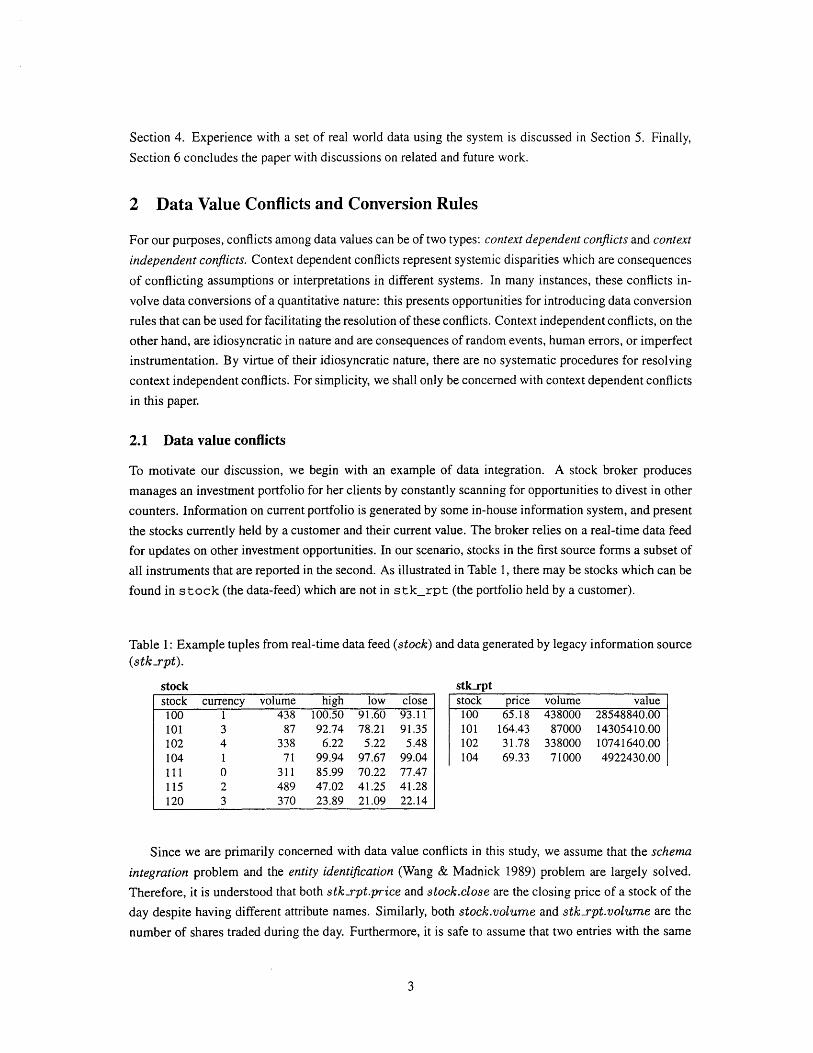
all instruments that are reported in the second. As illustrated in Table 1, there may be stocks which can be

found in stock (the data-feed) which are not in stkrpt (the portfolio held by a customer).

Table 1: Example tuples from real-time data feed (stock) and data generated by legacy information source(stk..rpt).

stockstock currency volume high low close

stk-rptstock price volume value

100 1 438 100.50 91.60 93.11 100 65.18 438000 28548840.00101 3 87 92.74 78.21 91.35 101 164.43 87000 14305410.00102 4 338 6.22 5.22 5.48 102 31.78 338000 10741640.00104 1 71 99.94 97.67 99.04 104 69.33 71000 4922430.00111 0 311 85.99 70.22 77.47115 2 489 47.02 41.25 41.28120 3 370 23.89 21.09 22.14

Since we are primarily concerned with data value conflicts in this study, we assume that the schema

integration problem and the entity identification (Wang & Madnick 1989) problem are largely solved.

Therefore, it is understood that both stk-rpt.price and stock.close are the closing price of a stock of the

day despite having different attribute names. Similarly, both stock.volume and stk-rpt.volume are the

number of shares traded during the day. Furthermore, it is safe to assume that two entries with the same

key (stock) value refer to the same company's stock. For example, tuple with stock = 100 in relation

stock and tuple with stock = 100 in relation stk-rpt refer to the same stock.

With these assumptions, it will be reasonable to expect that, for a tuple ss c stock and a tuple

tjt E stk-rpt, if s.stock = t.stock, then s.close = t.price and s.volume = t.volume. However, from

the sample data, this does not hold. In other words, data value conflicts exist among two data sources. In

general, we can define data value conflicts as follows.

Definition Given two data sources DS1 and DS 2 and two attributes A1 and A 2 that refer to

the same property of a real world entity type in DS 1 and DS 2 respectively, if ti E DS1 and

t2 E DS2 correspond to the same real world object but t1 .A1 $ t 2 .A 2, then we say that a

data value conflict exists between DS 1 and DS 2 .

In the above definition, attributes A1 and A 2 are often referred as semantically equivalent attributes.

We refer to the conflict in attribute values as value conflicts.j Value conflicts is therefore a form of seman-

tic conflict and may occur when similarly defined attributes take on different values in different databases,

including synonyms, homonyms, different coding schemes, incomplete information, recording errors,

different system generated surrogates and synchronous updates (see (Sheth & Kashyap 1992) for a classi-

fication of the various incompatibility problems in heterogeneous databases).

While a detailed classification of various conflicts or incompatibility problems may be of theoretical

importance to some, it is also true that over-classification may introduce unnecessary complexity that are

not useful for finding solutions to the problem. We adopt instead the Occam's razor in this instance and

suggest that data value conflicts among data sources can be classified into two categories: context depen-

dent and context independent. Context dependent conflicts exist because data from different sources are

stored and manipulated under different context, defined by the systems and applications, including phys-

ical data representation and database design considerations. Most conflicts mentioned above, including

different data type and formats, units, and granularity, synonyms, different coding schemes are context

dependent conflicts. On the other hand, context independent conflicts are those conflicts caused by some-

how random factors, such as erroneous input, hardware and software malfunctions, asynchronous updates,

database state changes caused by external factors, etc. It can be seen that context independent conflicts

are caused by poor quality control at some data sources. Such conflicts would not exist if the data are

"manufactured" in accordance to the specifications of their owner. On the contrary, data values involving

context dependent conflicts are perfectly good data in their respective systems and applications.

The rationale for our classification scheme lies in the observation that the two types of conflicts com-

mand different strategies for their resolution. Context independent conflicts are more or less random and

non-deterministic, hence cannot be resolved systematically or automatically. For example, it is very dif-

ficult, if not impossible, to define a mapping which can correct typographical errors. Human intervention

and ad hoc methods are probably the best strategy for resolving such conflicts. On the contrary, context de-

pendent conflicts have more predictable behavior. They are uniformly reflected among all corresponding

real world instances in the underlying data sources. Once a context dependent conflict has been identified,

it is possible to establish some mapping function that allows the conflict to be resolved automatically. For

example, a simple unit conversion function can be used to resolve scaling conflicts, and synonyms can be

resolved using mapping tables.

2.2 Data value conversion rules

In this subsection, we define data value conversion rules (or simply conversion rules) which are used

for describing quantitative relationships among the attribute values from multiple data sources. For ease

of exposition, we shall adopt the notation of Datalog for representing these conversion rules. Thus, a

conversion rule takes the form head +- body. The head of the rule is a predicate representing a relation

in one data source. The body of a rule is a conjunction of a number of predicates, which can either be

extensional relations present in underlying data sources, or builtin predicates representing arithmetic or

aggregate functions. Some examples of data conversion rules are described below.

Example: For the example given at the beginning of this section, we can have:

stk..rpt(stock, price, volume, value) +-

exchange-rate(currency, rate), stock(stock, currency, volume-in-K, high, low, close),price = close * rate, volume = volume-inI( * 1000, value = price * volume.

Example: For conflicts caused by synonyms or different representations, it is always possible to

create lookup tables which forms part of the conversion rules. For example, to integrate the data from

two relations Di.student(sid, sname, major) and D2.employee(eid, ename, salary), into a new relation

D1 .std-emp(id, name, major; salary), we can have a rule

D1 .std-emp(id, name, major; salary) <-

D1.student(id, name, major), D2 .employee(eid, name, salary), D1.same-person(ideid).

where same-person is a relation that defines the correspondence between the student id and employee

id. When the size of the lookup table is small, it can be defined as rules without bodies. One widely cited

example of conflicts among student grade points and scores can be specified by the following set of rules:

D1 .student(id, name, grade) +- D2.student(id, name, score), score-grade(score, grade).

score-grade(4, 'A').

score-grade(3, 'B').

score-grade(2, 'C').

score-grade(1, 'D').

score-grade(0, 'F').

One important type of conflicts mentioned in literature in business applications is aggregation con-

flict (Kashyap & Sheth 1996). Aggregation conflicts arise when an aggregation is used in one database to

identify a set of entities in another database. To be able to define conversion rules for attributes involving

aggregation conflicts, we can extend the traditional datalog to include aggregate functions. For example,

sales-summary(part, sales) +- sales(date, customer, part, amount), sales = SUM(part, amount).

can be used to resolve the conflicts between sales-summary and sales, where sales-summary.sales

is the total sales for a particular part in the sales table. Here, SUM(part, amount) is an aggregate func-

tion with two arguments. Attribute part is the group - by attribute and amount is the attribute on

which the aggregate function applies. In general, an aggregate function can take n + 1 attributes where

the last attribute is used in the aggregation and others represent the "group-by" attributes. For example,

if the sales.summary is defined as the relation containing the total sales of different parts to different

customers. The conversion rule could be defined as follows:

sales-summary(part, customer; sales) <-

sales(date, customer part, amount), sales = SUM(part, customer; amount).

We like to emphasize that it is not our intention to argue about appropriate notations for data value

conversion rules and their respective expressive power. For different application domains, the complex-

ity of quantitative relationships among conflicting attributes could vary dramatically and this will require

conversion rules having different expressive power (and complexity). The research reported here is pri-

marily driven by problems reported for the financial and business domains; for these types of applications,

a simple Datalog-like representation has been shown to provide more than adequate representations. For

other applications (e.g., in the realm of scientific data), the form of rules could be extended. Whatever the

case may be, the framework set forth in this paper can be used profitably to identify conversion rules that

are used for specifying the relationships among attribute values involving context dependent conflicts.

3 Mining Conversion Rules from Data

In this section, we describe our approach for circumventing semantic conflicts is to discover data conver-

sion rules from data that are redundantly present in multiple overlapping data sources. The methodology

underlying this approach is depicted schematically in Figure 1 and has been implemented in a prototype

system. The system consists of two subsystems: Data Preparation and Rule Mining. The data preparation

subsystem prepares a data set - the training data set - to be used in the rule mining process. The rule

mining subsystem analyzes the training data to generate candidate conversion functions. The data value

conversion rules are then formed using the selected conversion functions.

3.1 Training data preparation

The objective of this subsystem is to form a training data set to be used in the subsequent mining pro-

cess. The training data set should contain a sufficient number of tuples from two data sources with value

conflicts, that is, tuples referring to the same real world entity but having different values for the same

property (attribute).

To determine if two tuples ti, ti E DSi and t2 , t 2 E DS 2 represent the same real world entity is

an entity identification problem. In some cases, this problem can be easily resolved. For example, the

common keys of entities, such as a person's social security number and a company's registration number,

can be used to identify the person or the company in most of the cases. However, in large number of cases,

entity identification is still a rather difficult problem (Lim, Srivastava, Shekhar & Richardson 1993, Wang

& Madnick 1989). To determine whether two attributes Ai and A2 in ti and t2 model the same property of

the entity is sometimes referred to as the attribute equivalence problem. This problem has received much

attention in the schema integration literature (see for instance, (Chatterjee & Segev 1991, Larson, Navathe

Data Preparation Rule Mining

nemra inna M e l

nega i. D:ata

Source Reorganizion

ODBC Training Relvyn Caddate Conversion Cnversio Conversion

- ~JDBC Generation Analysis Selection Generation Selec1io Forrnation

Figure 1: Discovering data value conversion rules from data

& Elmasri 1989, Litwin & A.Abdellatif 1986)). One of the major difficulties in identifying equivalent

attributes lies in the fact that the anomaly cannot be simply determined by the syntactic or structural

information of the attributes. Two attributes modeling the same property may have different names and

different structures but two attributes modeling different properties can have the same name and same

structures.

In our study, we will not address the entity identification problem and assume that the data to be

integrated have common identifiers so that tuples with the same key represent the same real world entity.

This assumption is not unreasonable if we are dealing with a specific application domain. Especially for

training data set, we can verify the data manually in the worst case. As for attribute equivalence, as we

can see later, the rule mining process has to implicitly solve part of the problem.

3.2 Data value conversion rule mining

Like any knowledge discovery process, the process of mining data value conversion rules is a complex

one. More importantly, the techniques to be used could vary dramatically depending on the application

domain and what is known about the data sources. In this subsection, we will only briefly discuss each

of the modules. A specific implementation for financial and business data based on statistical techniques

will be discussed in the next section.

As shown in Figure 1 the rule mining process consists of the following major modules: Relevant

Attribute Analysis, Candidate Model Selection, Conversion Function Generation, Conversion Function

Selection, and Conversion Rule Formation. In case no satisfactory conversion functions are discovered,

training data is reorganized and the mining process is re-applied to confirm that there indeed no functions

exist. The system also tries to learn from the mining process by storing used model and discovered

functions in a database to assist later mining activities.

3.2.1 Relevant attribute analysis

The first step of the mining process is to find sets of relevant attributes. These are either attributes that are

semantically equivalent or those required for determining the values of semantically equivalent attributes.

As mentioned earlier, semantically equivalent attributes refer to those attributes that model the same prop-

erty of an entity type. In the previous stock and stkrpt example, stock.close and stk-rpt.price are

semantically equivalent attributes because both of them represent the last trading price of the day. On the

other hand, stock.high (stock.low) and stk.rpt.price are not semantically equivalent, although both of

them represent prices of a stock, have the same data type and domain.

The process of solving this attribute equivalence problem can be conducted at two levels: at the meta-

data level or at the data level. At the metadata level, equivalent attributes can be identified by analyzing

the available metadata, such as the name of the attributes, the data type, the descriptions of the attributes,

etc. DELTA is an example of such a system (Benkley, Fandozzi, Housman & Woodhouse 1995). It

uses the available metadata about attributes and converts them into text strings. Finding corresponding

attributes becomes a process of searching for similar patterns in text strings. Attribute equivalence can

also be discovered by analyzing the data. An example of such a system is SemInt (Wen-Syan Li 1994),

where corresponding attributes from multiple databases are identified by analyzing the data using neural

networks. In statistics, techniques have been developed to find correlations among variables of different

data types. In our implementation described in the next section, partial correlation analysis is used to find

correlated numeric attributes. Of course, equivalent attributes could be part of available metadata. In this

case, the analysis becomes a simple retrieval of relevant metadata.

In addition to finding the semantically equivalent attributes, the relevant attributes also include those

attributes required to resolve the data value conflicts. Most of the time, both metadata and data would

contain some useful information about attributes. For example, in relation stock, the attribute currency

in fact contains certain information related to attributes low, high and close. Such informative attributes

are often useful in resolving data value conflicts. The relevant attribute sets should also contain such

attributes.

3.2.2 Conversion function generation

With a given set of relevant attributes, {A 1 , ...Ak, B1 , ...B1} with A1 and B1 being semantically equivalent

attributes, the conversion function to be discovered

A1 = f (B1, ..., B1, A 2 ,...,Ak) (1)

should hold for all tuples in the training data set. The conversion function should also hold for other unseen

data from the same sources. This problem is essentially the same as the problem of learning quantitative

laws from the given data set, which has been a classic research area in machine learning. Various systems

have been reported in the literature (Langley, Simon, G.Bradshaw & Zytkow 1987, Kokar 1986, Wu &

Wang 1991, Zytkow & Baker 1991) Statisticians have also developed both theories and sophisticated

techniques to solve the problems of associations among variables and prediction of values of dependent

variables from the values of independent variables.

Most of the systems and techniques require some prior knowledge about the relationships to be discov-

ered, which is usually referred as models. With the given models, the data points are tested to see whether

the data fit the models. Those models that provide the minimum errors will be identified as discovered

laws or functions. We divided the task into two modules, the candidate model selection and conversion

function generation. The first module focuses on searching for potential models for the data from which

the conversion functions are to be discovered. Those models may contain certain undefined parameters.

The main task of the second module is to have efficient algorithms to determine the values of the param-

eters and the goodness of the candidate models in these models. The techniques developed in other fields

could be used in both modules. User knowledge can also be incorporated into the system. For example,

the model base is used to store potential models for data in different domains so that the candidate model

selection module can search the database to build the candidate models.

3.2.3 Conversion function selection and conversion rule formation

It is often the case that the mining process generates more than one conversion functions because it is

usually difficult for the system to determine the optimal ones. The conversion function selection module

needs to develop some measurement or heuristics to select the conversion functions from the candidates.

With the selected functions, some syntactic transformations are applied to form the data conversion rules

as specified in Section 2.

3.2.4 Training data reorganization

It is possible that no satisfactory conversion function is discovered with a given relevant attribute set be-

cause no such conversion function exists. However, there is another possibility from our observations:

the conflict cannot be reconciled using a single function, but is reconcilable using a suitable collection of

different functions. To accommodate for this possibility, our approach includes a training data reorgani-

zation module. The training data set is reorganized whenever a single suitable conversion function cannot

be found. The reorganization process usually partitions the data into a number of partitions. The mining

process is then applied in attempting to identify appropriate functions for each of the partition taken one at

a time. This partitioning can be done in a number of different ways by using simple heuristics or complex

clustering techniques. In the case of our implementation (to be described in the next section), a simple

heuristic of partitioning the data set based on categorical attributes present in the data set is used. The

rationale is, if multiple functions exist for different partitions of data, data records in the same partition

must have some common property, which may be reflected by values assumed by some attributes within

the data being investigated.

4 DIRECT: A Prototype System

The strategy which we have described in the preceding section has been implemented in a prototype

system, DIRECT (DIscovering and REconciling ConflicTs), thus allowing the proposed methodology

and techniques to be verified both experimentally and in the context of a real application. The system is

developed with a focus on financial and business data for a number of reasons. First, the relationships

among the attribute values for financial and business data are relatively simpler compared to engineering

or scientific data. Most relationships are linear or products of attributes. 5 Second, business data do have

some complex factors. Most monetary figures in business data are rounded up to the unit of currency.

Such rounding errors can be viewed as noises that are mixed with the value conflicts caused by context.

As such, our focus is to develop a system that can discover conversion rules from data with noises. The

basic techniques used are from statistics and the core part of the system is implemented using S-Plus, a

programming environment for data analysis. In this section, we describe the major statistical techniques

used in the system.

4.1 The basic techniques

DIRECT uses Partial Correlation Analysis (PCA) to identify relevant attributes since it is well known

that properly used, partial correlation analysis can uncover spurious relationships, identify intervening

variables, and detect hidden relationships that are present in a data set.

It is important to take note that correlation and semantic equivalence are two different concepts. A

person's height and weight may be highly correlated, but are semantically distinct. However, since se-

mantic conflicts arise from differences in the representation schemes and these differences are uniformly

applied to each entity, we expect a high correlation to exist among the values of semantically equivalent

attributes. Partial correlation analysis can at least isolate the attributes that are likely to be related to one

another for further analysis.

In order to discover quantitative relationships among the identified relevant attributes, another well

known statistical technique, regression analysis is implement in DIRECT. To deal with noises in data, such

as rounding errors, we implemented the Least Trimmed Squares (LTS) regression method (Rousseeuw &

Hubert 1997). LTS regression, unlike the traditional Least Square (LS) regression that tries to minimize

the sum of squared residuals of all data points, minimizes a subset of the ordered squared residuals, and

leave out those large squared residuals, thereby allowing the fit to stay away from those outliers and

leverage points. Compared with other robust techniques, like Least Median Sqaure (LMS) regression,

LTS also has a very high breakdown point: 50%. That is, it can still give a good estimation of model

parameters even half of the data points are contaminated. More importantly, a faster algorithm exists to

estimate the parameters (Bums 1992).

4.2 Bayesian information criterion based candidate model selection

Given a set of relevant attributes, a model is required before performing regression. The model specifies

the number of attributes that should actually be included and the basic relationship among them, e.g.,

linear, polynomial, logarithmic, and etc. There are a number of difficulties regarding selecting the model

for regression. First, with n independent attributes, a model can include 1 to n attributes with any com-

binations. That is, even just considering the linear functions, there could be a large number of possible

models. Second, it is often the case that, a given data set can fit into more than one model. Some of them

5Aggregation conflicts are not considered in this paper.

are equally good. Third, if there is in fact no valid model, the regression may still try to fit the data into

the model that may give the false impression that the relationship given is valid.

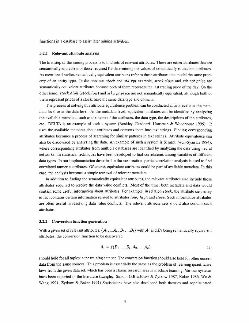
A number of techniques have been developed to automatically select and rank models from a set

of attributes (Miller 1990). Recently, Raftery introduced the BIC, Bayesian Information Criterion, an

approximate to Bayes factors used to compare two models based on Bayes's theorem (Raftery 1995). For

different regression functions, the BIC takes different forms. In the case of linear regression, BICk of a

model Mk can be computed as

BIC Nlog(1 - R2) + pklogN (2)

where N is the number of data points, R2 is the value of adjusted R2 for model Mk and pA is the number

of independent attributes. Using the BIC values of models, we can rank the models. The smaller the

BIC is, the better the model is to fit the data. One important principle in comparing two nested models

is so called Occam's Window. For two models, Mk and Mk+1 where k is the number of independent

attributes. The essential idea is that, if Mk is better than Mk+1, model Mk+1 is removed. However, if

model Mk+1 is better, it requires a certain "difference" between two models to cause Mk to be removed.

That is, there is an area, the Occam's Window, where Mk+1 is better than Mk but not better enough to

cause Mk being removed. The size of Occam's Window can be adjusted. Smaller Occam's Window size

will cause more models to be removed, as we can see from the example given in the next subsection. The

following procedure highlights this candidate model selection process.

1. Given a set of relevant attributes, form the candidate model set by including all possible models;

2. From the candidate model set, remove all the models that are vastly inferior compared to the model

which provides the best prediction;

3. Remove those models which receive less support from the data than any of their simpler submodels,

i.e., models with less independent attributes;

4. Whenever a model is removed from the candidate model set in the above two steps, all its submodels

are also removed.

4.3 Acceptance criteria of generated conversion functions

Since regression can always generate some conversion functions given a data set, one key issue in our

implementation is to find the criteria that can be used to determine the genuine conversion functions. To

address this issue of acceptance criterion, we defined a measure, support, to evaluate the goodness of a

discovered regression function (conversion function) based on recent work of Hoeting, Raftery and Madi-

gan (Hoeting, Raftery & Madigan 1995). A function generated from the regression analysis is accepted

as a conversion function only if its support is greater than a user specified threshold -y. The support of a

regression function is defined as

Count{yfl(round(lyi - yll)/scale) <= E}support = N (3)

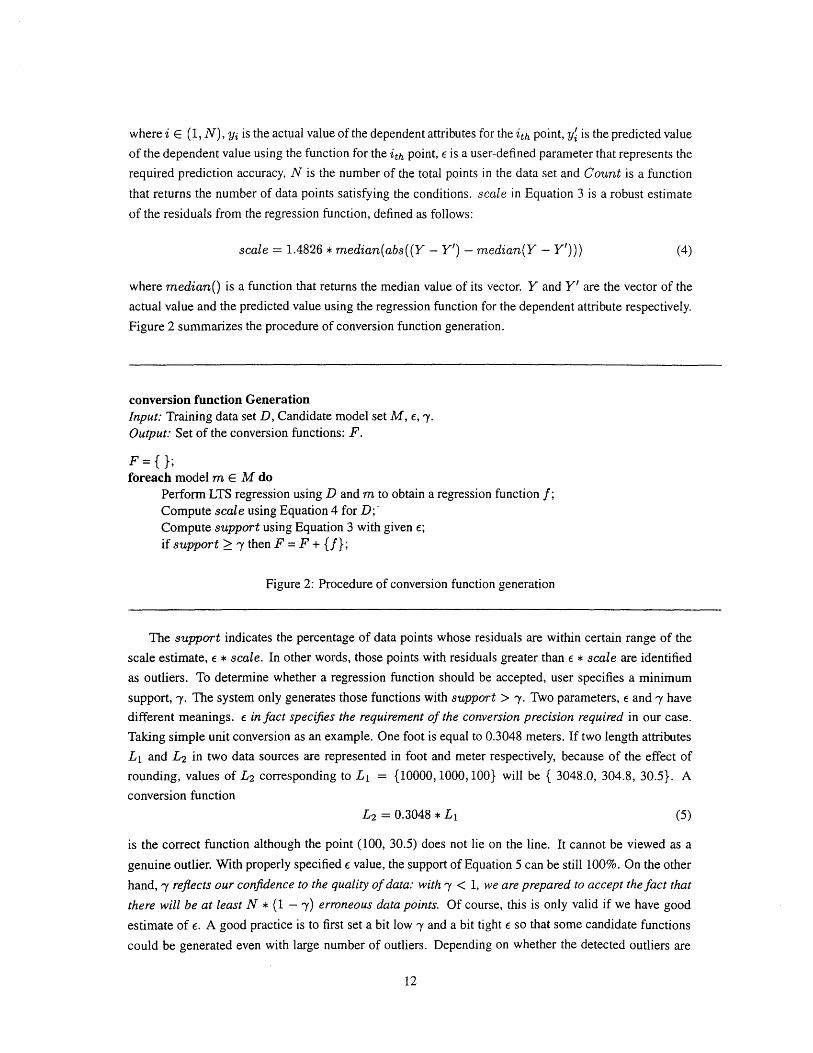
where i E (1, N), yj is the actual value of the dependent attributes for the Zth point, y is the predicted value

of the dependent value using the function for the sth point, e is a user-defined parameter that represents the

required prediction accuracy, N is the number of the total points in the data set and Count is a function

that returns the number of data points satisfying the conditions. scale in Equation 3 is a robust estimate

of the residuals from the regression function, defined as follows:

scale = 1.4826 * median(abs((Y - Y') - median(Y - Y'))) (4)

where median() is a function that returns the median value of its vector. Y and Y' are the vector of the

actual value and the predicted value using the regression function for the dependent attribute respectively.

Figure 2 summarizes the procedure of conversion function generation.

conversion function GenerationInput: Training data set D, Candidate model set M, e, 7.Output: Set of the conversion functions: F.

F = { };foreach model m E M do

Perform LTS regression using D and m to obtain a regression function f;Compute scale using Equation 4 for D;Compute support using Equation 3 with given e;if support > -y then F = F + {f};

Figure 2: Procedure of conversion function generation

The support indicates the percentage of data points whose residuals are within certain range of the

scale estimate, e * scale. In other words, those points with residuals greater than e * scale are identified

as outliers. To determine whether a regression function should be accepted, user specifies a minimum

support, 7. The system only generates those functions with support > -y. Two parameters, e and -y have

different meanings. e in fact specifies the requirement of the conversion precision required in our case.

Taking simple unit conversion as an example. One foot is equal to 0.3048 meters. If two length attributes

Li and L 2 in two data sources are represented in foot and meter respectively, because of the effect of

rounding, values of L 2 corresponding to Li = {10000, 1000, 100} will be { 3048.0, 304.8, 30.5}. A

conversion function

L2 =0.3048 * Li (5)

is the correct function although the point (100, 30.5) does not lie on the line. It cannot be viewed as a

genuine outlier. With properly specified e value, the support of Equation 5 can be still 100%. On the other

hand, y reflects our confidence to the quality of data: with - < 1, we are prepared to accept the fact that

there will be at least N * (1 - y) erroneous data points. Of course, this is only valid if we have good

estimate of e. A good practice is to first set a bit low y and a bit tight e so that some candidate functions

could be generated even with large number of outliers. Depending on whether the detected outliers are

genuine outliers or data points still with acceptable accuracy, the value of c and -y can be adjusted.

4.4 A running example with synthetic data

To illustrate the workings of the prototype system, we present here the detailed results obtained from

DIRECT when a synthetic data set is used as the training data. The data set simulates the stock data

integration process mentioned at the beginning in this paper: A broker receives stock information and

integrates it into his/her own stock report. For this experiment, we created a data set of 6000 tuples. The

attributes and their domain are listed in Table 2

Table 2: Example relations

Attr. No. Relation Name Value RangeAl stock, stk..rpt scode [1, 500]A2 stk-rpt price stock.close*exchange-rate(stock.currency]A3 stk.rpt volume stock.volume * 1000A4 stk-rpt value stk.rpt.price * stk.rpt.volumeA5 stock currency 1, 2, 3, 4, 5, randomA6 stock volume 20-500, uniform distributionA7 stock high [stock.close, 1.2*stock.close]A8 stock low [0.85*stock.close, stock.close]A9 stock close [0.50, 100], uniform distribution

4.4.1 Relevant attribute analysis

The zero-order correlation analysis was first applied to the training data. If the correlation efficient be-

tween two attributes is greater than the threshold, which was set to 0.1 in the experiment, they were

considered relevant. The results and relevant attribute sets are shown in Table 3.

Table 3: Correlation coefficients from the zero-Order correlation analysis

A6 A7 A8 A9A2 0.0291 0.3933 0.4006 0.4050A3 1.0000 -0.0403 -0.0438 -0.0434A4 0.3691 0.2946 0.2994 0.3051

Set Attribute Correlated Attributes1 A3 A62 A4 A6, A7, A8, A93 A2 A7, A8, A9

Partial correlation analysis was conducted by controlling A6, A7, A8 and A9 in turn to see whether

there are more attributes that should be included in the obtained relevant attribute sets. In this example,

there were no such attributes; and the relevant attribute sets remained the same.

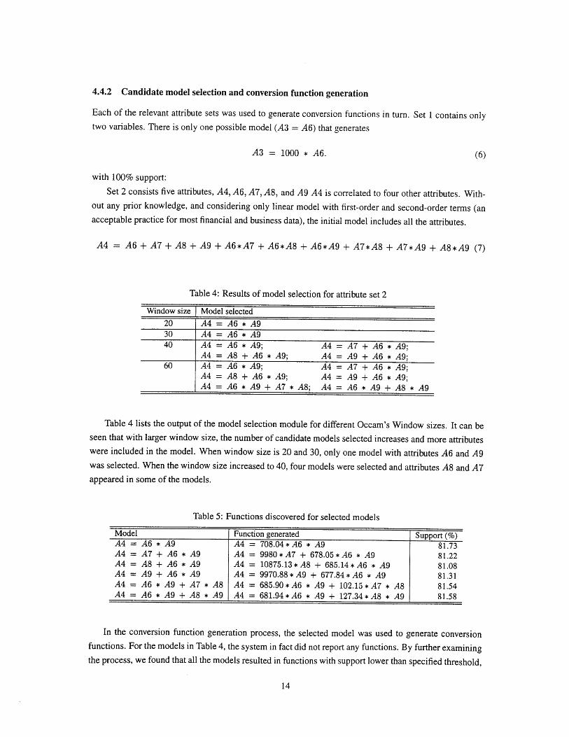
4.4.2 Candidate model selection and conversion function generation

Each of the relevant attribute sets was used to generate conversion functions in turn. Set 1 contains onlytwo variables. There is only one possible model (A3 = A6) that generates

A3 = 1000 * A6.

with 100% support:

Set 2 consists five attributes, A4, A6, A7, A8, and A9 A4 is correlated to four other attributes. With-out any prior knowledge, and considering only linear model with first-order and second-order terms (anacceptable practice for most financial and business data), the initial model includes all the attributes.

A4 = A6 + A7 + A8 + A9 + A6*A7 + A6*A8 + A6*A9 + A7*A8 + A7*A9 + A8*A9 (7)

Table 4: Results of model selection for attribute set 2

Window size Model selected20 A4 = A6 * A930 A4 = A6 * A940 A4 = A6 * A9; A4 = A7 + A6 * A9;

A4 = A8 + A6 * A9; A4 = A9 + A6 * A9;60 A4 = A6 * A9; A4 = A7 + A6 * A9;

A4 = A8 + A6 * A9; A4 = A9 + A6 * A9;AA = A * A9 + A7 * A8; A4 = A6 * A9 + A8 * A9

Table 4 lists the output of the model selection module for different Occam's Window sizes. It can beseen that with larger window size, the number of candidate models selected increases and more attributeswere included in the model. When window size is 20 and 30, only one model with attributes A6 and A9was selected. When the window size increased to 40, four models were selected and attributes A8 and A7appeared in some of the models.

Table 5: Functions discovered for selected models

Model Function generated SupportA4 = A6 * A9 A4 = 708.04*A * A9 81.73A4 = A7 + A6 * A9 A4 = 9980*A7 + 678.05*A * A9 81.22A4 = A8 + A6 * A9 A4 = 10875.13*A8 + 685.14*A6 A9 81.08A4 = A9 + A6 * A9 A4 = 9970-88*A9 + 677.84*A6 A9 81.31A4 = A * A9 + A7 * A A4 = 68590*A6 * A + 102.15 *A7 * A8 81.54A4 = A6 * A9 + A8 * A9 A4 = 681.94 * A6 * A9 + 127.34 * A8 * A9 81.58

In the conversion function generation process, the selected model was used to generate conversionfunctions. For the models in Table 4, the system in fact did not report any functions. By further examiningthe process, we found that all the models resulted in functions with support lower than specified threshold,

Table 5.

As illustrated in Figure 1, when a selected model does not generate any single conversion function

with sufficient support, there is a possibility that there exist multiple functions for the data set. To discover

such multiple functions, the data set should be reorganized. In our implementation, a simple heuristic is

used, that is, to partition the data using categorical attributes in the data set. After the data was partitioned

based on a categorical attribute A5, the model selected are shown in Table 6.

Table 6: Models selected for partitioned data

Window size Model selected20 A4 = A6 * A940 A4 = A6 * A960 A4 = A6 * A9; A4 = A6 + A6 * A9;

A4 = A7 + A6 * A9; A4 = A8 + A6 * A9;A4 = A9 + A6 * A9; A4 = A6 * A7 + A6 * A9;A4 = A6 * A8 + A6 * A9; A4 = A6 * A9 + A7 * A8;A4 = A6 * A9 + A7 * A9; A4 = A6 * A9 + A8 * A9

The conversion function generation module estimates the coefficients for each of the models selected

for each partition. There is only one conversion function reported for each partition, since all the coeffi-

cients for the terms other than A6 * A9 were zero. The results are summarize in Table 7.

Table 7: The conversion functions generated from Set 2 and 3

Conversion functions for A4A5 Conversion function Support (%)_

0 A4 = 400 * A6 * A9 1001 A4 = 700 * A6 * A9 1002 A4 = 1000 * A6 *A9 1003 A4 = 1800 * A6 *A9 1004 A4 = 5800 * A6* A9 100

Conversion functions for A2A5 Conversion function Support (%)0 A2 = 0.4 * A9 1001 A2 = 0.7 * A9 1002 A2 = 1.0 * A9 1003 A2 = 1.8 * A9 1004 A2 = 5.8 * A9 100

The process for relevant attribute Set 3: {A2, A7, A8, A9} is similar to what described for Set 2. The

initial model used is

A2 = A7 + A8 + A9 + A7 * A8 + A7 * A9 + A8 * A9

and the model selection module selected 10 models without producing functions with enough support.

Using the data sets partitioned using A5 and the conversion functions listed in Table 7 were obtained.

4.4.3 Conversion function selection and data conversion rule formation

Since there is only one set of candidate functions obtained for each set of relevant attribute set with 100%

support. The functions generated were selected to form the data conversion rules. By some syntactic

transformation, we can obtain the following data conversion rules for our example:

stk-rpt(stock, price, rpt-volume, value) +-

stock(stock, currency, stkvolume, high, low, close),

price = rate * close, rpt-volume = 1000 * stk-volume,

value = rate * 1000 * stk-volume * close, exchange _rate(currency, rate).

exchange-rate(0, 0.4).

exchange-rate(1, 0.7).

exchange-rate(2, 1.0).

exchange.rate(3, 1.8).

exchange-rate(4, 5.8).

It is obvious that the discovered rule can be used to integrate data from stock to stk-rpt.

5 Experience with a real world data set

In this section, we present the experimental results on a set of real world data using the system described in

the previous section. The motivation for this exercise is to demonstrate that the techniques and framework

remain applicable in the context of a real-world application.

The data used in this experiment was collected from a trading company. Each record consists of 10

attributes. Attribute Al to A8 are from a transaction database, T(month, invoice-no, amount, sales-type,

GST-rate, currency, exchange-rate, GST-amount), which records the details of each invoice billed, hence

all the amounts involved are in the original currency. Attribute A9, C.amount is extracted from a system

for cost/profit analysis, which captures the sales figure in local currency exclusive of tax. Finally, attribute

A10, A.amorunt, is from the accounting department, A, where all the monetary figures are in the local

currency. Therefore, although attributes A3, A9 and A10 have the same semantics, i.e., all refer to the

amount billed in an invoice, their values are different. That is, value conflict exists among the attributes.

From the context of the business, the following relationship among the attributes should exist:

A.amount = T.amount * T.exchange..rate. (9)

C.amount = (T.amount - T.GST-amount) * T.exchange-rate (10)

= A.amount - T.exchange-rate * T.GSTamount. (11)

The goods and service tax (GST), is computed based on the amount charged for the sales of goods or

services. As C.amount is in the local currency and all transaction data are in the original currency, we

have the following relationship:

T.GST-amount = C.amount/T.exchange-r ate * T.GST -rate (12)

where GST rate depends on the nature of business and clients. For example, exports are exempted from

GST (tax rate is 0%) and domestic sales are taxed in a fixed rate of 3% in our case.

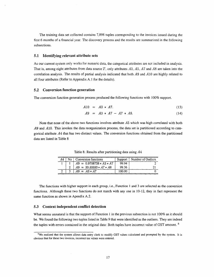
The training data set collected contains 7,898 tuples corresponding to the invoices issued during the

first 6 months of a financial year. The discovery process and the results are summarized in the following

subsections.

5.1 Identifying relevant attribute sets

As our current system only works for numeric data, the categorical attributes are not included in analysis.

That is, among eight attributes from data source T, only attributes A3, A5, A7 and A8 are taken into the

correlation analysis. The results of partial analysis indicated that both A9 and A10 are highly related to

all four attributes (Refer to Appendix A. 1 for the details).

5.2 Conversion function generation

The conversion function generation process produced the following functions with 100% support.

A10 = A3 * A7. (13)

A9 = A3 * A7 - A7 * A8. (14)

Note that none of the above two functions involves attribute A5 which was high correlated with both

A9 and A10. This invokes the data reorganization process, the data set is partitioned according to cate-

gorical attribute A4 that has two distinct values. The conversion functions obtained from the partitioned

data are listed in Table 8

Table 8: Results after partitioning data using A4

A4 No Conversion functions Support Number of Outliers1 1 A9 = 0.9708738 * A3 * A7 99.94 2

2 A9 = 33.33333 * A7 * A8 99.36 212 3 A9 = A3* A7 100.00 0

The functions with higher support in each group, i.e., Function 1 and 3 are selected as the conversion

functions. Although these two functions do not match with any one in 10-12, they in fact represent the

same function as shown in Apendix A.2.

5.3 Context independent conflict detection

What seems unnatural is that the support of Function 1 in the previous subsection is not 100% as it should

be. We found the following two tuples listed in Table 9 that were identified as the outliers. They are indeed

the tuples with errors contained in the original data: Both tuples have incorrect value of GST amount. 6

6We realized that the system allows data entry clerk to modify GST values calculated and prompted by the system. It isobvious that for these two invoices, incorrect tax values were entered.

Table 9: Two erroneous tuple discovered

month inv-no amt. GST type GST rate currency exch. rate GST C.amount A.amount3 8237 45.50 1 3 1 1.00 0.00 45.50 45.506 12991 311.03 1 3 1 1.00 6.53 304.50 311.03

5.4 Applying the discovered function to test data

In order to verify the functions obtained, the sales data of the 7th month containing 1,472 tuples were

collected. We applied discovered functions to calculate A9 and A10. It was found that there was no

difference between the values calculated using the discovered functions and the values collected from the

databases.

5.5 Discussion

From the experimental results of the real world data set, we made the following observations.

1. In the systems from which the sales data were collected, the exchange rate has 6 digits after the

decimal point. All other computed amount has only 2 digits after the decimal point. Furthermore,

a number of attributes are derived by a number of arithmetic operations. Therefore, the data values

contain rounding errors introduced during calculations. In addition to the rounding errors, the data

set also contains two error entries. Under our classification, the data set contains both context

dependent and context independent conflicts.

Our first conclusion is this: although the training data set contains noises (rounding errors) and both

context dependent and independent conflicts (two outliers), the system was still able to discover the

correct conversion functions.

2. One interesting function discovered by the system but not selected (eventually) is Function 2 in

Table 8. Note that, from the expression itself, it is derivable from the other correct functions: Since

A8 is the amount of tax in the original currency, A9 is the amount of sales in the local currency, A7

is the exchange rate, and A5 is the tax rate(percentage), we have

A9A8 = -- *0.01 * A5

A7

That is,A7 *A8

A 9 = A7 5 for A5 : 00.01 * A5

When A4 = 1, A5 = 3, so we should have

A7* A8A9 = = 33.33333 * A7 * A8.

0.01 * 3

which is the same as Function 2. The function was discarded because of its low support (99.36%).

It seems puzzling that a function that is derivable from the correct functions has such low support

so that it should be discarded.

It turns out that this phenomenon can be explained. Since, the derivation process is purely mathe-

matical, it does not take into any consideration how the original data value is computed. In the real

data set, the tax amount stored has been rounded up to 0.01. The rounding error may get propagated

and enlarged when Function 2 is used. If exchange rate is 1.00 (i.e., the invoice is in the local cur-

rency), the possible error of A9 introduced by using Function 2 to compute the sales amount from

the tax amount could be as large as 33.33333*0.005. This is much larger than the precision of A9

which is 0.005. To verify the reasoning, we modified the function into

A9= A7*A8 = 33.33333 * A7 * roundup(A8)0.01 * 3

where roundup is a function that rounds A8 to 0.01; and calculated A9 using the modified function.

Comparing the calculated values and the corresponding values in the data set, the differences for all

tuples are less than 0.005.

This leads to our second conclusion: because noises such as rounding errors existing in the data

and different ways in which the original data were produced, we should not expect a conversion

function mining system to reproduce the functions that are used in generating the original data. The

objective of such systems is to find the functions that data from multiple sources can be integrated

or exchanged with specified requirement of accuracy.

6 Conclusion

In this paper, we addressed the problem of discovering and resolving data value conflicts for data inte-

gration. We first proposed a simple classification scheme for data value conflicts based on how they can

be reconciled. We argue that those conflicts caused by genuine semantic heterogeneity can be reconciled

systematically using data value conversion rules. A general approach for discovering data conversion rules

from data was proposed. statistical techniques are integrated in to a prototype system to implement the

approach for financial and business data. The system was tested using some both synthetic and real world

data.

The approach advocated in this paper identify conversion rules which are defined on data sources on

a pairwise basis (i.e., between any two systems at a time). One drawback of this is that we may have to

be defined a large number of rules if a large number of sources are involved. It will be beneficial if we

are able to go a step further to to elicit meta-data information from conversion rules obtained. This will

allow us to introduce appropriate meta-data tags to each of the data source while allowing postponing the

decision of which conversion rule should be applied (Bressan, Fynn, Goh, Jakobisiak, Hussein, Kon, Lee,

Madnick, Pena, Qu, Shum & Siegel 1997). This will be advantageous because it will help reduce the

volume of information that the underlying context mediator has to deal with. For example, in the example

given in Section 5, the conversion rules only indicate the ways to compute the sales and tax based on tax

rate. It would be more economical if we are able to match the tax rate to yet another data source furnishing

the sales type and tax rate and figure out that different sales have different tax by virtual of the type of

sales. Thus, if we know that all sales in a company have been charged 3% tax, we can conclude that the

company only has domestic sales.

References

Agarwal, S., Keller, A. M., Wiederhold, G. & Saraswat, K. (1995), Flexible relation: An approach for integrating

data from multiple, possibly inconsistent databases, in 'Proc. IEEE Intl Conf on Data Engineering', Taipei,

Taiwan.

Benkley, S., Fandozzi, J., Housman, E. & Woodhouse, G. (1995), Data element tool-based analysis (delta), Technical

Report MTR 95B0000147, The MITRE Corporation, Bedford, MA.

Bressan, S., Fynn, K., Goh, C. H., Jakobisiak, M., Hussein, K., Kon, H., Lee, T., Madnick, S., Pena, T., Qu, J., Shum,

A. & Siegel, M. (1997), The COntext INterchange mediator prototype, in 'Proc. ACM SIGMOD/PODS Joint

Conference', Tuczon, AZ.

Bums, P. (1992), 'A genetic algorithm for robust regression estimation', StatScience Technical Note.

Chatterjee, A. & Segev, A. (1991), 'Data manipulation in heterogeneous databases', ACM SIGMOD Record

20(4), 64-68.

Dayal, U. (1983), Processing queries with over generalized hierarchies in a multidatabase system, in 'Proceedings

of VLDB Conference', pp. 342-353.

Demichiel, L. G. (1989), 'Resolving database incompatibility: an approach to performing relational operations over

mismatched domains', IEEE Trans on Knowledge and Data Engineering 1(4), 485-493.

Hoeting, J., Raftery, A. & Madigan, D. (1995), A method for simultaneous variable selection and outlier identifica-

tion, Technical Report 9502, Department of Statistics, Colorado State University.

Kashyap, V. & Sheth, A. (1996), 'Schematic and semantic similarities between database objects: A context-based

approach', VLDB Journal 5(4).

Kokar, M. (1986), 'Determining arguments of invariant functional description', Machine Learning 4(1), 403-422.

Langley, P., Simon, H., G.Bradshaw & Zytkow, M. (1987), Scientific Discovery: An Account of the Creative Pro-

cesses, MIT Press.

Larson, J., Navathe, S. & Elmasri, R. (1989), 'A theory of attribute equivalence in databases with application to

schema integration', IEEE Software Engineering 15(4), 449-463.

Lim, E.-P., Srivastava, J. & Shekhar, S. (1996), 'An evidential reasoning approach to attribute value conflict resolu-

tion in database integration', IEEE Transactions on Knowledge and Data Engineering 8(5).

Lim, E.-P., Srivastava, J., Shekhar, S. & Richardson, J. (1993), Entity identification problem in database integration,

in 'Proceedings of the 9th IEEE Data Engineering Conference', pp. 294-301.

Litwin, W. & A.Abdellatif (1986), 'Multidatabase interoperability', Computing 19(12), 10-18.

Miller, A. (1990), Subset Selection in Regression, Chapman and Hall.

Raftery, A. (1995), 'Bayesian model selection in social research', Sociological Methodology pp. 111-196.

Rousseeuw, P. & Hubert, M. (1997), Recent developments in progress, in 'Ll-Statistical Procedures and Related

Topics', Vol. 31, Institute of Mathematical Statistics Lecture Notes-Monograph Series, Hayward, California,pp. 201-214.

Scheuermann, P. & Chong, E. I. (1994), Role-based query processing in multidatabse systems, in 'Proceedings of

International Conference on Extending Database Technology', pp. 95-108.

Scheuermann, P., Li, W.-S. & Clifton, C. (1996), Dynamic integration and query processing with ranked role sets,

in 'Proc. First International Conference on Interoperable and Cooperative Systems (CoopIS'96)', Brussels,

Belgium, pp. 157-166.

Sciore, E., Siegel, M. & Rosenthal, A. (1994), 'Using semantic values to facilitate interoperability among heteroge-

neous information systems', ACM Transactions on Database Systems 19(2), 254-290.

Sheth, A. & Kashyap, V. (1992), So far (schematically) yet so near (semantically), in D. K. Hsiao, E. J. Neuhold

& R. Sacks-Davis, eds, 'Proceedings of the IFIP WG2.6 Database Semantics Conference on Interoperable

Database Systems (DS-5)', North-Holland, Lorne, Victoria, Australis, pp. 283-312.

Tseng, F. S., Chen, A. L. & Yang, W.-P. (1993), 'Answering heterogeneous databse queries with degrees of uncer-

tainty', Distributed and Parallel Databases: An International Jounal 1(3), 281-302.

Wang, Y. R. & Madnick, S. E. (1989), The inter-database instance identification problem in integrating autonomous

systems, in 'Proceedings of the Sixth International Conference on Data Engineering'.

Wen-Syan Li, C. C. (1994), Semantic integration in heterogeneous databases using neural networks, in 'Proceedings

of the 20th VLDB Conference', pp. 1-12.

Wu, Y & Wang, S. (1991), Discovering functional relationships from observational data, in 'Knowledge Discovery

in Databases', The AAAI Press.

2ytkow, J. & Baker, J. (1991), Interactive mining of regularities in databases, in 'Knowledge Discovery in

Databases', The AAAI Press.

Appendix A: Results with Real World Data

A.1 Results of partial correlation analysis

The following table lists the results of the partial correlation analysis. Note that, the correlation coefficients between

A10 and A5, A10 and A7 are rather small in the zero-order test. However, this alone is not sufficient to conclude

that A10 is not related to A5 and A7. By the PCA test with controlling A3, the correlation between A10 and A7

became rather obvious and the correlation coefficient between A10 and A5 also increased. With one more PCA

test that controls A8, the correlation between A10 and A5 became more obvious. Thus, all the four attributes are

included into the quantitative relationship analysis.

Table 10: Partial correlation analysis between A10 and {A3,A5,A7,A8}

Correlation Efficient of Al0 with

Zero-order Controlling A3 Controlling A8

A3 0.91778708 - 0.8727613A5 0.02049382 0.1453855 -0.2968708A7 0.02492715 0.4562510 -0.006394451A8 0.71552943 0.5122901 -

Table 11: Partial correlation analysis between A9 and {A3,A5,A7,A8}

Correlation Efficient of A9 withZero-order Controlling A3 Controlling A8

A3 0.91953641 - 0.8739174A5 0.01350388 0.1292704 -0.2976056A7 0.02355110 0.4581783 -0.007597317A8 0.70452050 0.4791232

A.2: Tests with partitioned data

In this section, we show the detailed deduction that the functions generated for A9,

A9 = 0.9708738 * A3 * A7

A9 = A3 * A7

conform the original functions.

Using the attribute numbers instead of the name, we can rewrite Equation 11 as

A9 = A3 * A7 - A8 * A7

The tax rate, A5, is stored as the percentage, Equation 12 can be rewritten as

A9A8 = * 0.01* A5

A7

(15)

(16)

Thus we have

A9A9 = A3*A7- *0.01*A5*A7A7

= A3*A7-0.01*A9*A5

Therefore,eA9 A3 * A7 (17)

1 + 0.01 * A5

From the data, we have

A5 = 3 forA4 = 10 for A4 = 2

Substituting this into Equation 17, we have

A9= A3.7 = 0.9708738 * A3 * A7 for A4 = 1A3* A7 for A4 = 2

which are the functions 16 and 16. In other words, although the two functions have different forms, they do

represent the original relationship among the data values specified by Equation 17.