Embed Size (px)
Citation preview
Discovering During-Temporal Patterns (DTPs)
in Large Temporal Databases ∗
Li Zhanga, Guoqing Chena,†, Tom Brijsb, Xing Zhanga
a School of Economic and Management, Tsinghua University, Beijing, 100084, P.R.China
b Transportation Research Institute, Hasselt University, Diepenbeek, B3920, Belgium
Abstract Large temporal Databases (TDBs) usually contain a wealth of data about tem-
poral events. Aimed at discovering temporal patterns with during relationship (during-temporal
patterns, DTPs), which is deemed common and potentially valuable in real-world applications,
this paper presents an approach to finding such DTPs by investigating some of their properties
and incorporating them as desirable pruning strategies into the corresponding algorithm, so as
to optimize the mining process. Results from synthetic reveal that the algorithm is efficient and
linearly scalable with regard to the number of temporal events. Finally, we apply the algorithm
into the weather forecast field and obtain effective results.
Keywords: data mining; during relationship; temporal pattern
1 Introduction
In recent years, discovery of association rules [14] and sequential patterns [13] has been a major
research issue in the area of data mining. While typical association rules usually reflect related events
occurring at the same time, sequential patterns represent commonly occurring sequences that are in a
time order. However, real-world businesses often generate a massive volume of data in daily operations
and decision-making processes, which are of a richer temporal nature. For instance, a customer could
buy a DVD machine after TV was bought; the duration of an ERP project partially overlapped the
duration of a BPR project; and a patient suffered from cough during the period of fever. Apparently,∗The work was partly supported by the National Natural Science Foundation of China (70231010/70321001), Tsinghua
University’s Research Center for Contemporary Management, and the Bilateral Scientific and Technological Cooperationbetween China and the Flanders.
†Corresponding author.E-Mail: [email protected]. edu.cn
1
such temporal relationships (e.g., after, overlap, during, etc.) are kinds of real-world semantics that
are, in many cases, considered meaningful and useful in practice. Usually, temporal relationships
between events with different time stamps could be categorized into several types in forms of temporal
comparison predicates such as after, meet, overlap, during, start, finish, and equal [10]. Though recent
years have witnessed several efforts on discovering the after relationship [7,8,11,13], more in-depth
investigations of the relationship are still badly needed, let along their explorations of other types of
temporal relationships. Furthermore, results from the studies on the after relationship could hardly
be simply extended to the case of some other relationships such as during, overlap, etc. This may be
attributed to the fact that in the after relationship, events can generally be dealt with on a time point,
whereas in other relationships, events are considered to be of a time interval nature.
On the other hand, both Rainsford [3] and Hoppner [6] have recently discussed the issues of finding
temporal relationships between time-interval-based events using temporal comparison predicates [10],
but with different mining approaches. Rainsford introduced temporal semantics into association rules,
in forms of X⇒Y∧P1∧P2∧...∧Pn (n≥0), where X and Y are itemsets, and X ∩Y = ∅. P1∧P2∧...∧Pn
is a conjunction of binary temporal predicates. While mining a database DT , a rule is accepted
when its confidence factor 0≤c≤1 is equal to or larger than the given threshold. Similarly, each
predicate Pi is measured with a temporal confidence factor 0≤tcPi≤1. The algorithm firstly generates
the traditional association rules without considering the temporal factors, and then finds all of the
possible pairings of temporal items in each rule. Subsequently, these pairings are tested so that
strong temporal relationships could be found. Obviously, the complexity of this sequentially executed
algorithm rises rapidly as the number of typical rules grows. Differently, Hoppner proposed another
technique for discovering temporal patterns in state sequences. He defined the supporting level of a
pattern as the total time in which the pattern can be observed within a sliding window, which should
be predetermined by the user. However, a major concern for this technique is how to decide a proper
size for the sliding window, since the sliding window can affect the mining results. Furthermore, The
changes of the sliding window will lead to a sub-patterns check. The check requires some backtracking
mechanism, which is computationally expensive. Like many existing data mining algorithms, the
algorithm needs to scan the database repeatedly, which would significantly lower its efficiency.
This paper will focus on a particular type of temporal relationships, namely during, which rep-
resents that one event starts and ends within the duration of another event. Notably, this during
relationship could reflect the temporal semantics of during, start, finish and equal described in [10].
An approach will be proposed to discover the so-called during-temporal patterns (DTPs) in larger
temporal databases, which are considered common and potentially valuable in real-world applications.
One idea behind the approach is to design the corresponding algorithm so as to reduce the workload in
2
scanning the database. In doing so, the database is partitioned into some disjoined datasets with two
operations when calculating the support level of each pattern, so that scanning the whole database
could be avoided. Furthermore, some properties of DTPs are investigated and then incorporated into
the algorithm as pruning strategies to optimize the mining process for efficiency purposes.
The remainder of this paper is organized as follows. Section 2 formulates the problem and introduces
related notions. In Section 3, the algorithmic details are provided, along with some of the related
properties. The experiments on synthetic data and real weather data are discussed in Section 4, and
Section 5 concludes the paper.
2 The problem formulation
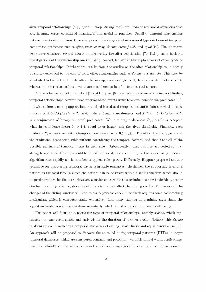
Let A={a1,a2,...,am} be a set of states, and DT a temporal database as shown in Table 1. Given
a database DT with N records, each of which is in the form of {a,(st,et)} with respect to event e,
i.e., e=(a,t), where a is the state involved in the event, t=(st,et) is the time interval which indicates
starting time (st) and ending time (et) of state a in the event. A specific event is denoted as el=(ai ,tl)
(1≤l≤N and 1≤i≤m) and tl = (stl , etl), i.e., S(el)=stl and E(el)=etl . For example, with a1=rain,
e1=(a1,(1,20)) in Table 1 means that it began to rain at 1:00h and ended at 20:00h.
Table 1: A Temporal DatabaseEvent State Starting Time Ending Time
e1 a1 1 20e2 a3 1 4e3 a4 5 7e4 a1 22 28e5 a2 2 8e6 a3 10 13e7 a5 25 35e8 a3 23 28e9 a4 25 27e10 a6 25 26e11 a1 30 40e12 a3 30 38e13 a4 34 38e14 a6 37 37
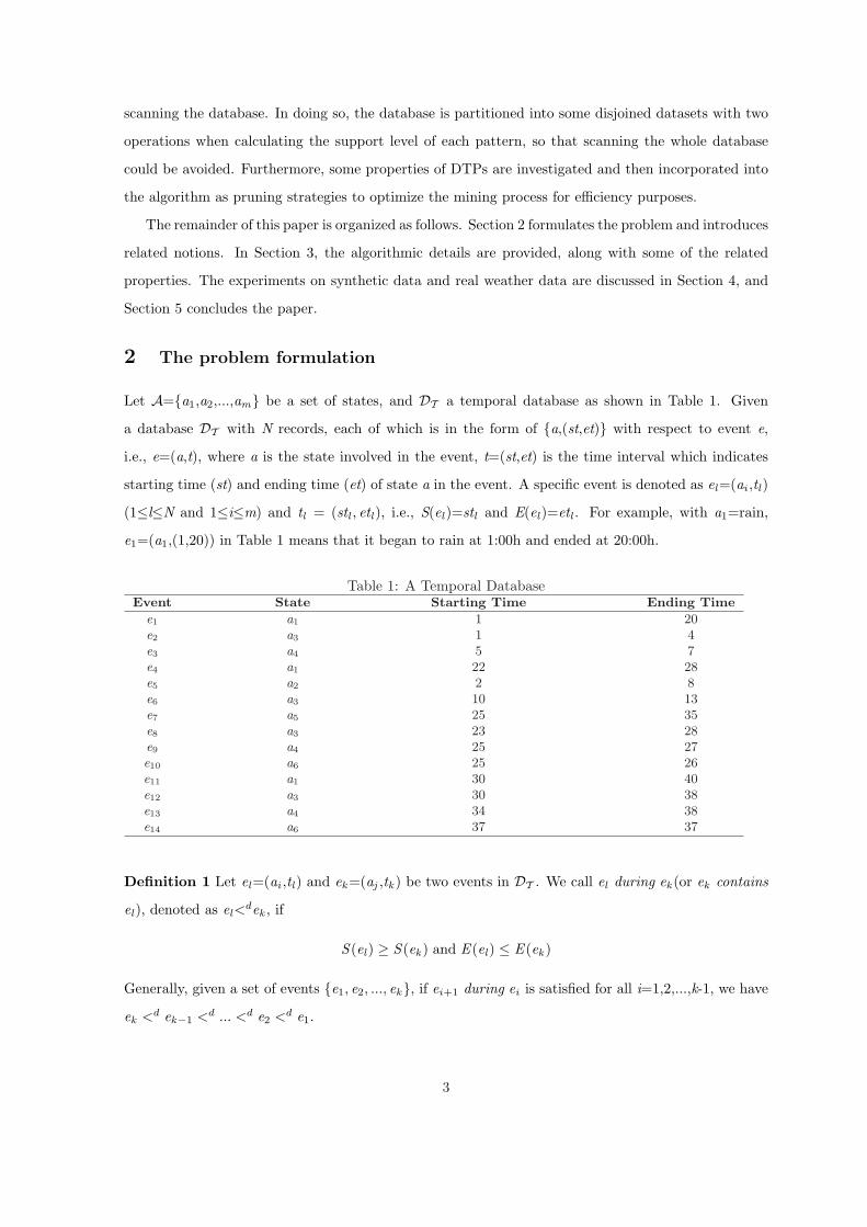
Definition 1 Let el=(ai ,tl) and ek=(aj ,tk ) be two events in DT . We call el during ek (or ek contains
el), denoted as el<dek , if
S (el) ≥ S (ek ) and E (el) ≤ E (ek )
Generally, given a set of events {e1, e2, ..., ek}, if ei+1 during ei is satisfied for all i=1,2,...,k-1, we have
ek <d ek−1 <d ... <d e2 <d e1.
3
For any two states ai and aj , ai is called to be during aj , denoted as pattern ai⇒daj , if state ai
occurs during the period of another state aj , which is a during-temporal pattern (DTP) with length
1. Generally, a DTP of length (k-1) (k≥1), namely DTPk−1, is of the form:
ak ⇒d ak−1 ⇒d ... ⇒d a2 ⇒d a1
When the length is 0 (i.e., DTP0), the pattern is a single state actually. More generally, given two
patterns α and β, the form α⇒dβ is also a DTP (Aα ∩ Aβ = ∅, where Aα and Aβ are the sets of
states included in pattern α and β respectively). As a special case, it retrogresses to ai⇒daj when the
lengths of both patterns are 0.
Given a pattern ak ⇒d ak−1 ⇒d ... ⇒d a2 ⇒d a1 , ek <d ek−1 <d ... <d e2 <d e1 supports this
pattern if ai is the state of ei for all i=1,2,...,k. In the case, ek <d ek−1 <d ... <d e2 <d e1 can be
considered as an instance of this pattern. For example, in Table 1, e10<de9<
de8 is an instance of the
pattern a6⇒da4⇒da3, and e14<de13<
de12 is another instance of this pattern. Further, a DTP α
ak ⇒d ak−1 ⇒d ... ⇒d aj+1 ⇒d aj ⇒d aj−1 ⇒d ... ⇒d a2 ⇒d a1
is characterized by the number of its instances: ek <d ek−1 <d ... <d e2 <d e1, and a DTP β ⇒d γ,
i.e.,
(ak ⇒d ak−1 ⇒d ... ⇒d aj+1) ⇒d (aj ⇒d aj−1 ⇒d ... ⇒d a2 ⇒d a1)(1 ≤ j ≤ k − 1)
is characterized by the number of its instances:
(ek <d ek−1 <d ... <d ej+1) <d (ej <d ej−1 <d ... <d e2 <d e1)
which is ek <d ek−1 <d ... <d ej+1 <d ej <d ej−1 <d ... <d e2 <d e1 according to the associative law
of events. Hence, β ⇒d γ equivalently reads
ak ⇒d ak−1 ⇒d ... ⇒d aj+1 ⇒d aj ⇒d aj−1 ⇒d ... ⇒d a2 ⇒d a1 (1 ≤ j ≤ k − 1)
Furthermore, for finding all instances of a DTP α, one may consider to scan the whole database.
In fact, however, only a small part of the database, with respect to the set of states included in α,
is useful. Thus, we can divide the database into m datasets (m is the number of the states in the
database), each of which is the set of time intervals of a single state. Thus, when finding all instances
of ak ⇒d ak−1 ⇒d ... ⇒d aj+1 ⇒d aj ⇒d aj−1 ⇒d ... ⇒d a2 ⇒d a1, only those datasets which include
the sets of time intervals of ak , ak−1, ..., a2, and a1 are scanned. For this purpose, we define a time
interval set g(α) and a state set h(α) to partition the database, and join the small datasets to count
the support (which will be discussed in this and next sections).
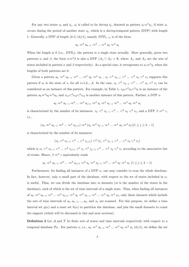
Definition 2 Let A and T be finite sets of states and time intervals respectively with respect to a
temporal database DT . For pattern α, i.e., ak ⇒d ak−1 ⇒d ... ⇒d a2 ⇒d a1 (k≥1), we define the set
4
of time intervals g(α) as the set of finest time intervals of all the instances of α. Formally, g(α) is the
function mapping the set of patterns to the set of time intervals,
g(α) = {t |(ai , t) ∈ DT }, if the length of α is 0, i.e., α is a single state ai .
g(α) = {tk ∈ g(ak )|for all i = 1, 2, ..., k − 1, ai ∈ Aα,∃ti ∈ g(ai), such that ti+1 ∩ ti = ti+1}, (2-1)
if the length of α is larger than 0. In the definition, tl ∩ tk = (max{stl , stk},min{etl , etk}).Equivalently, we have
g(α) = {tk |for each instance of α : ek (ak , tk ) <d ek−1(ak−1, tk−1) <d ... <d e1(a1, t1)} (2-2)
g(ai) includes all the intervals in which ai occurred, so all instances of α can be found using g(a1),
g(a2),...,g(ak ). And ti+1 ∩ ti = ti means ei+1 <d ei , for i=1,2,...,k-1. That is, ti+1 ∩ ti = ti for
i=1,2,...,k-1 means that ek (ak , tk ) <d ek−1(ak−1, tk−1) <d ... <d e2(a2, t2) <d e1(a1, t1). Hence, both
(2-1) and (2-2) get the set of finest time intervals of all the instances of α.
Support g(a1) h(a1)
1 (1,20)2 (22,28) a2,a3,a4,a6
3 (30,40)
Support g(a2) h(a2)
1 (2,8) a4
Support g(a3) h(a3)
1 (1,4)2 (10,13)3 (23,28)
a4,a6
4 (30,38)
(a) (b) (c)
Support g(a4) h(a4)
1 (5,7)2 (25,27) a6
3 (34,38)
Support g(a5) h(a5)
1 (25,35) a4,a6
Support g(a6) h(a6)
1 (25,26)2 (37,37)
∅
(d) (e) (f)
Support g(a3 ⇒d a1) h(α)
1 (1,4)(10,13)
2 (23,28)a4,a6
3 (30,38)
Support g(a4 ⇒d a1) h(α)
1 (5,7)2 (25,27) a3,a6
3 (34,38)
(g) (h)
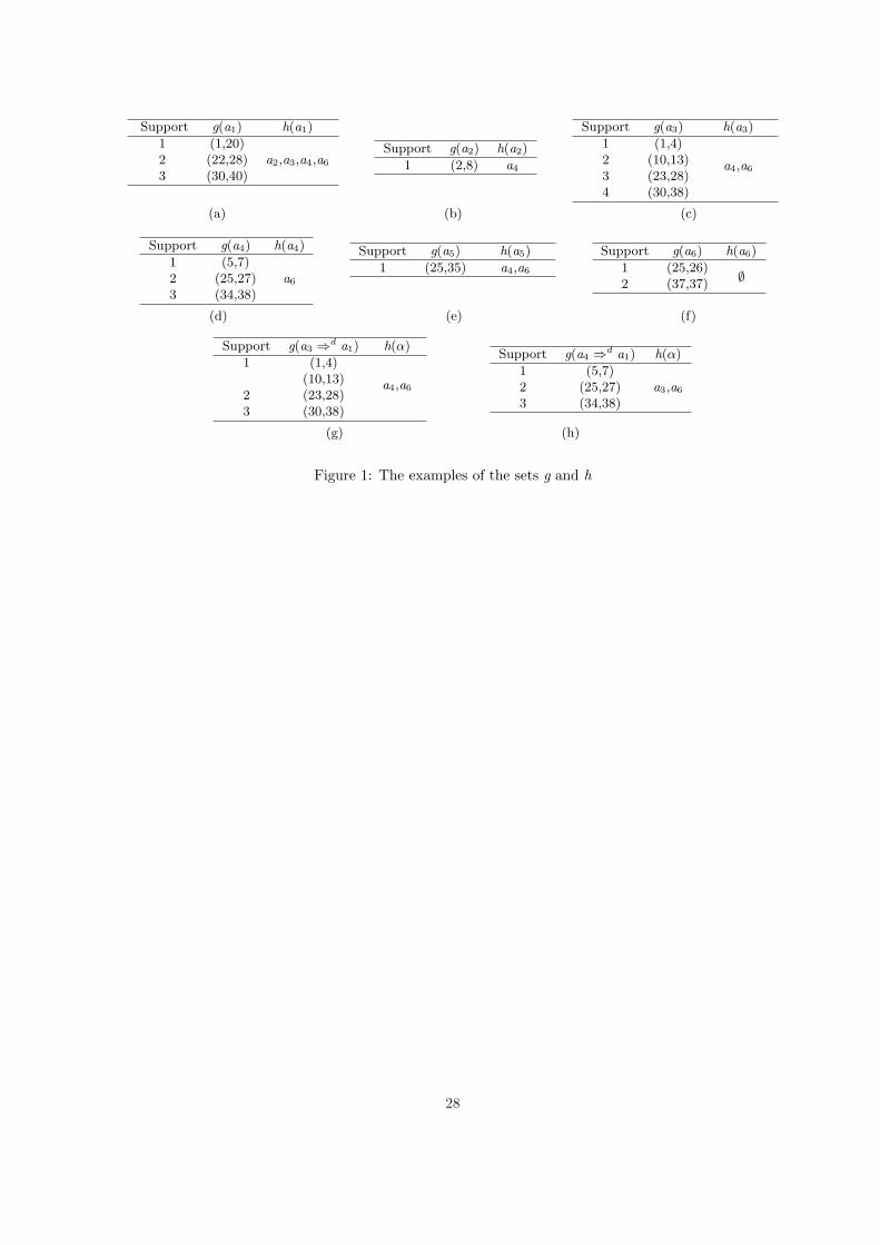
Figure 1: The examples of the sets g and h
For example, given a temporal database DT as shown in Table 1. g(a1)={(1,20), (22,28), (30,40)}and g(a3)={(1,4), (10,13), (23,28), (30,38)}. According to ti+1∩ti = ti+1 in (2-1), we have (1,4)∩(1,20)
=(1,4), (10,13)∩(1,20)=(10,13), (23,28)∩(22,28)=(23,28), and (30,38)∩(30,40)=(30,38), so g(a3 ⇒d
a1)={(1,4), (10,13), (23,28), (30,38)}. According to (2-2), we need to find these intervals from original
temporal database. The instances of a3 ⇒d a1 include e2 <d e1, e6 <d e1, e8 <d e4 and e12 <d e11,
which result in time intervals (1,4), (10,13), (23,28), and (30,38) respectively. That is, g(a3 ⇒d
5
a1)={(1,4), (10,13), (23,28), (30,38)}. More examples can be found in Figure 1. Next, we will define
the support degree of a DTP pattern (Definition 3).
Definition 3 The support degree of a DTP α is the fraction of the support count of the pattern. That
is,
support(α) = |g(α)||g0 |
where |g(α)| is the number of time intervals in g(α) without double-counting those intervals of the
instances in that an event contains several events with the same state, and |g0|= max{|g(ai)|, for
i=1,2,...,m}. Actually, |g(α)| is the number of instances supporting α without double-counting. α is
said to be frequent if the support degree is not less than the given threshold (i.e., minsupport).
The support degree of pattern α in Definition 3 is the ratio of the number of time intervals included
in all instances of α (without double-counting) over the maximum number of time intervals among
|g(ai)| for all i. In other words, support(α) reflects the relative frequency of time intervals for α with
respect to the number of time intervals for a most frequent state. In the first place, by ‘without double-
counting’ we mean that the instances with an event containing several events having the same state will
only be counted once, as they all support the same single pattern. In the second place, alternatively
g0 may be defined as N=∑m
i=1|g(ai)| , for the same purpose. However, since N=∑m
i=1|g(ai)| is usually
much larger than |g(α)|, it will result in too small values for support degrees. Therefore, a scale-
down measure is often considered desirable. As a matter of fact, other forms of g0 could be possible,
depending on the context and convenience. Notably, since g0 is a fixed number, the choice of it is a
technical treatment and does not affect the properties of DTPs. Take Table 1 as an example again. For
a DTP pattern α: a3⇒da1, we have |g(α)| =|{(1,4), (10,13), (23,28), (30,38)}|=3, and |g0|=4. Thus,
support(α)=3/4=0.75. Here, we have an event that contains several events with the same state. That
is, e1=(a1,(1,20)), e2=(a3,(1,4)), and e6=(a3,(10,13)), we have e2<de1 and e6<
de1, which contribute
to the same DTP a3⇒da1. This counting is also similar to that described in [2].
t
a3
a2 a2
a1
a3
a2
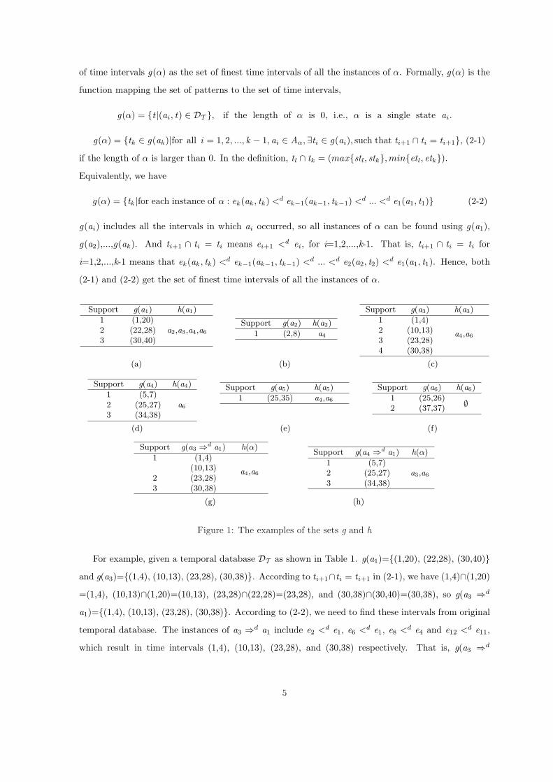
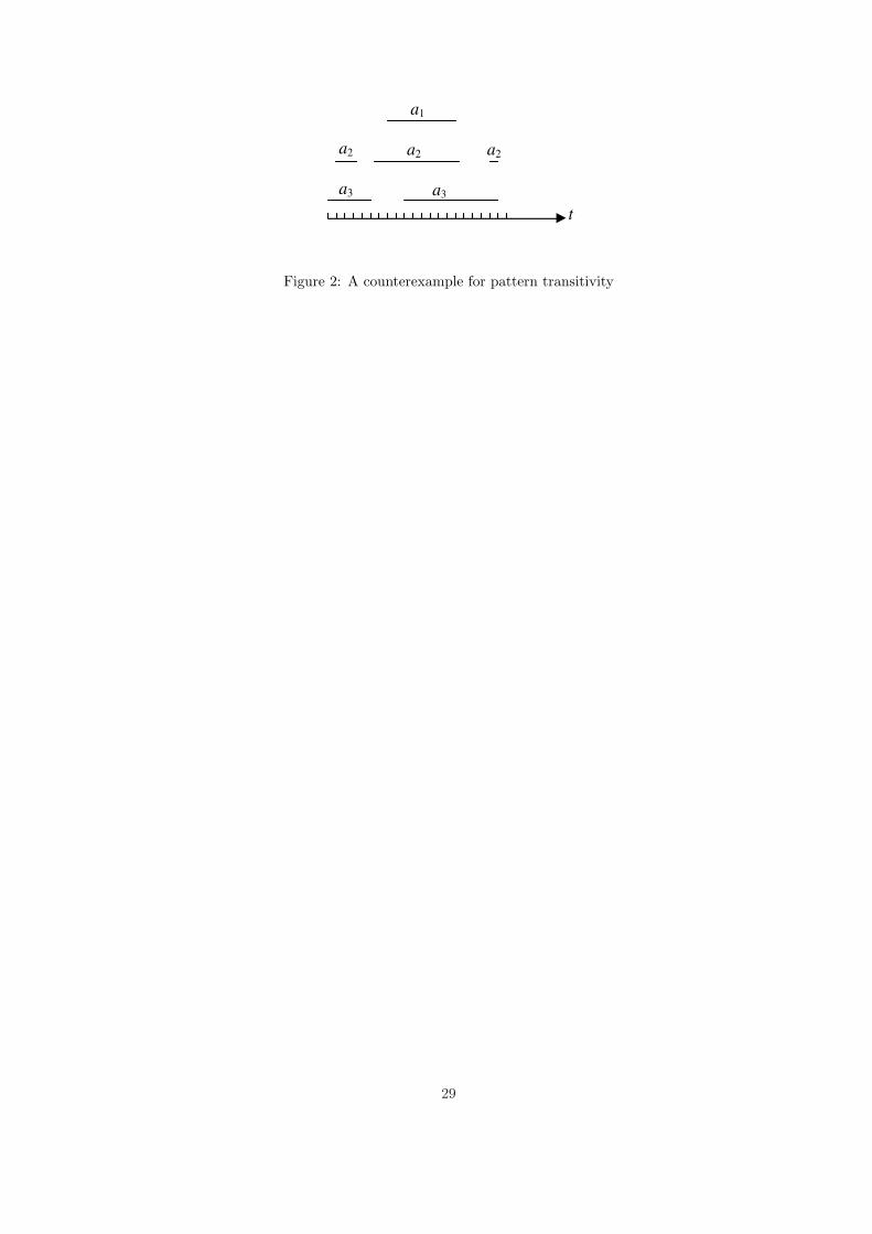
Figure 2: A counterexample for pattern transitivity
Note that the transitivity for during relationships between events exists. That is, if e <d e p
and e p <d eq, then we have e <d eq. For instance, we have e10<de9 and e9<
de8 in Table 1, and
e10<de9<
de8. However, it is worth mentioning that the during relationship are not transitive between
6

patterns in terms of support degree. Let us consider an example as follows. Given a temporal database
DT ={(a3,(1,5)), (a2,(2,4), (a2,(6,15)), (a1,(8,15)), (a3,(10,20)), (a2,(20,20))} and minimal support
count=1, with time intervals for the events being illustrated in Figure 2, we have |g(a1 ⇒d a2)|=1,
|g(a2 ⇒d a3)|=2, but |g(a1 ⇒d a3)|=0. Thus, we cannot obtain longer patterns from short ones using
transitivity. This gives rise to the effort to find other ways of generating longer patters. First, in
examining whether DTPs are frequent, we may need to consider sub-patterns. Definition 4 introduces
the notion.
Definition 4 For a DTP α with length l, we say that α is a sub-DTP of another DTP β with length
k, denoted as α¹β if l≤k and there exists an order-preserving mapping ϕ: {1,2,...,l}→{1,2,...,k} such
that
α(1) ⇒d α(2) ⇒d ... ⇒d α(l) is the same to β(ϕ(1)) ⇒d β(ϕ(2)) ⇒d ... ⇒d β(ϕ(l))
where α(i) is the ith state in the pattern α.
For instance, a6⇒da4⇒da1 is one of sub-DTPs of the pattern a6⇒da4⇒da3⇒da1. Moreover, we
say g(α)⊇g(β) if for every tk∈g(β) there exists a time interval tl∈g(α) such that tl ∩ tk = tk . In terms
of events, g(α)⊇g(β) means that for every event ek with tk in g(β), there exists an event el with tl in
g(α) such that ek<del .
Note that g(α)⊇g(β) does not necessarily mean |g(α)|≥|g(β)|. For example, as shown in Figure 1,
g(a1)⊇g(a3) but |g(a1)|<|g(a3)|. Importantly, for two DTPs α and β with α¹β, one could expect that
a longer DTP in length will have a less chance of being supported than its sub-DTPs since the longer
the length, the fewer its supporting instances in the database. Accordingly, the fewer the supporting
instances for a longer DTP, the finer the set that contains the time intervals of the longer DTP. These
statements are proved in Property 1.
Property 1 if α¹β, then g(α)⊇g(β) and |g(α)|≥|g(β)| .
Proof: Suppose that g(α)⊇g(β) does not hold. Therefore, there exists at least a time interval
tk∈g(β), such that tl∩tk 6=tk for all tl∈g(α). According to the definition about the set g, every state in
Aβ is active in tk . However, not all the states in Aα are active in tk since tk cannot be totally contained
by any interval in g(α). That is, some states in Aβ are not active in tk since α¹β and Aα⊆Aβ . This
is a contradiction with tk∈g(Aβ). That is, there must be g(α)⊇g(β) if α¹β.
Furthermore, each time interval tk∈g(β) is contained by the corresponding interval tl∈g(α) since
g(α)⊇g(β). Some tl could contain several tk , and some could not contain any tk . Let |g(α)|=x,
{T1,T2,...,Tx} be the set of time interval sets, in which Ti(i=1,2,...,x) represents the set of time
intervals contributing only once for the support count. Let the variable yi be the flag which represents
whether a new instance without double-counting is found in Ti . If a new instance without double-
7
counting has been found, then yi=1. Otherwise, yi=0. Thus,
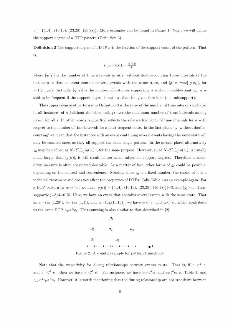
|g(β)| = ∑xi=1yi ≤ x × 1 = x = |g(α)| ¥
Property 2 All subsets of a frequent pattern are frequent.
Proof: Let β be a frequent pattern, and α is a sub-DTP of β. Thus, we have support(β)≥minsupport
according to Definition 3, and
|g(α)|≥|g(β)|according to Property 1. That is, support(α)≥support(β)≥minsupport, which means that α is frequent.
¥
The above two properties are very important in the process of finding frequent patterns. Effort in
scanning the database and examining longer DTPs could then be largely saved by only concentrating
on those frequent (sub-)patterns. This is because any DTP containing a non-frequent sub-DTP will
not be frequent.
A frequent pattern means that it occurs in forms of events in a sufficient level of frequency. Usually,
one also needs to know how likely a pattern occurs given that the other pattern has already occurred.
In other words, we are considering the notion of confidence. Concretely, given two DTPs β and γ,
where β=ak ⇒d ak−1 ⇒d ... ⇒d aj+1 of length (k-j-1) and γ=aj ⇒d aj−1 ⇒d ... ⇒d a2 ⇒d a1 of
length (j-1)for j={1,2,,k-1}. Then β during γ is a composition of these two DTPs as β⇒dγ which
forms a DTP α as follows:
α : (ak ⇒d ak−1 ⇒d ... ⇒d aj+1) ⇒d (aj ⇒d aj−1 ⇒d ... ⇒d a2 ⇒d a1)
= ak ⇒d ak−1 ⇒d ... ⇒d aj+1 ⇒d aj ⇒d aj−1 ⇒d ... ⇒d a2 ⇒d a1
Definition 5 The confidence degree of a DTP α: β⇒dγ is defined as the fraction of the support of
pattern α over the support of the consequent pattern γ.
confidence(α) = support(α)support(γ) = |g(α)|
|g(γ)|
The DTP β⇒dγ is a valid DTP if the support and confidence degrees exceed the corresponding
thresholds (minsupport and minconfidence).
Consider Figure 1 again as an example with β and γ being of length 0, i.e., β=a3 and γ=a1.
confidence(a3 ⇒d a1) = support(a3 ⇒d a1)/support({a1})=3/3=1.
Finally, given a DTP α (i.e., ak ⇒d ak−1 ⇒d ... ⇒d a2 ⇒d a1(k≥1)), let us consider a set of states
occurring during the period a1 excluding those states already contained by Aα. The state in the set
8
shall be during a1 in a frequent manner. Concretely, such a set, h(α), is defined as:
h(α) = {aj |aj 6∈ Aα, j =1, 2, ..., k , and if α is of a lengh ≥ 1 then
aj ⇒d a1, support(aj ⇒d a1) ≥ minsuport}
The set h(α) will be used conveniently in the process of generating candidate DTPs, which will be
discussed in detail in the following sections. Merely for illustrative purposes, in Figure 1, we have, for
example, h(a1)={a2,a3,a4,a6}. In comparison, we have h(a3 ⇒d a1)={a4,a6} where a2 is not included
since a2⇒da1 is not frequent, and a3 is not included either since a3 is already in Aα.
3 The algorithm
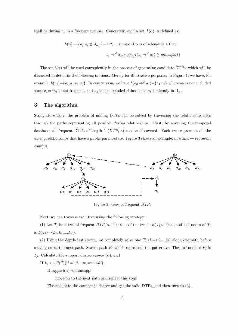
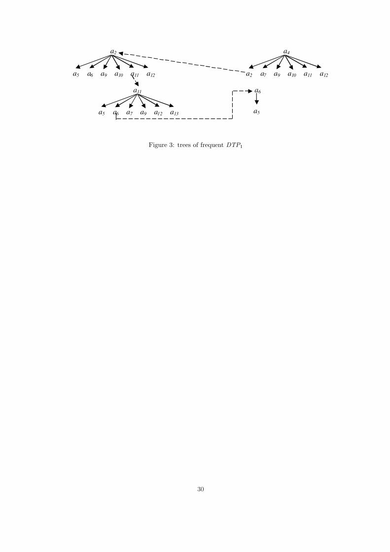
Straightforwardly, the problem of mining DTPs can be solved by traversing the relationship trees
through the paths representing all possible during relationships. First, by scanning the temporal
database, all frequent DTPs of length 1 (DTP1ps) can be discovered. Each tree represents all the
during relationships that have a public parent-state. Figure 3 shows an example, in which → represent
contain.
a2
a5 a6 a9 a10 a11 a12
a6
a5
a4
a2 a7 a9 a10 a11 a12
a11
a5 a6 a7 a9 a12 a13
Figure 3: trees of frequent DTP1
Next, we can traverse each tree using the following strategy:
(1) Let Tl be a tree of frequent DTP1ps. The root of the tree is R(Tl). The set of leaf nodes of Tl
is L(Tl)={L1,L2,...,Ln}.(2) Using the depth-first search, we completely solve one Tl (l =1,2,...,m) along one path before
moving on to the next path. Search path Pj which represents the pattern α. The leaf node of Pj is
Lj . Calculate the support degree support(α), and
If Lj ∈ {R(Ti)|i =1,2,..,m, and i6=l},If support(α) < minsupp,
move on to the next path and repeat this step.
Else calculate the confidence degree and get the valid DTPs, and then turn to (3).
9
Else move on to the next path and turn to (2).
(3)Consider the leaf nodes of Ti which are child nodes of Lj in Ti , i.e., L(Tl(Lj ))={L(Ti}, the
new tree T ′l is generated, T ′
l =Tl⊕L(Tl(Lj )), where ⊕ is an operation that treats all leaf nodes of Ti
as the child nodes of Lj in and forms the new tree T ′l . Thus, path Pj is extended as a sub-tree, which
represents several DTPs. Turn to (2). Stop it until no new tree is generated.
Take Figure 3 as an example. For the tree with the root being a4, and Pj : a4→a2, we process the tree
in the following order a4→a2, a4→a2→a5, a4→a2→a6,a4→a2→a6→a5..., a4→a2→a11, a4→a2→a11→a5,
a4→a2→a11→a6, a4→a2→a11→a6 →a5, and so on.
Note that this algorithm firstly finds the DTPs by traversing the trees in the way of depth-first
search such that Property 1 can be applied. However, it needs to enumerate all possible candidate
DTPs from DTP1 and will consume much time. The method is referred to as Tree algorithm for
distinguishing and comparing with the optimized approach that is to propose in the next subsections.
3.1 DTP Algorithm
To tackle the above problem, we propose a new algorithm, namely the DTP algorithm, which works
in an iterative manner by alternating between the joining and pruning phases, after finding frequent
DTP0ps. As the first step, support levels of all single states DTP0
ps are calculated and frequent single
state patterns are found. Meanwhile, the whole database DT is divided into m p (m p≤m) parts (m p
frequent single states). Secondly, in the join phase of an iteration k, a collection CDTPk of new
candidate patterns with length k is generated from the set of frequent DTPk−1ps(FDTPk−1). Thirdly,
the collection FDTPk of new frequent DTPk−1ps are generated by computing the support degrees.
Lastly, the patterns satisfying the confidence threshold are output after all iterations are terminated.
More concretely, the algorithmic details are described as follows.
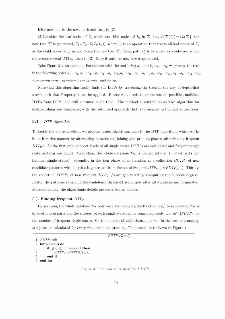
(1). Finding frequent DTP0
By scanning the whole database DT only once and applying the function g(ai) to each event, DT is
divided into m parts and the support of each single state can be computed easily. Let m p=|FDTP0| be
the number of frequent single states. So, the number of valid datasets is m p. In the second scanning,
h(ai) can be calculated for every frequent single state ai . The procedure is shown in Figure 4.
FDTP0.Gen()1. FDTP0=∅;2. for all ai∈A do3. if |g(ai)|≥ minsupport then4. FDTP0=FDTP0∪{ai};5. end if6. end for
Figure 4: The procedure used for FDTP0
10

(2). Join phase
The algorithm employs an iterative approach known as a level-wise search, where FDTPk−1 is used
to explore FDTPk (k≥1). First, the set of frequent DTP0(namely FDTP0) is found. FDTP0 is used to
find FDTP1, which is used to find FDTP2, and so forth, until no more frequent pattern can be found.
The generation of each frequent pattern carries a search cost. To improve the efficiency of generating
frequent patterns, two properties are presented as follows.
Let p(α,l) be a sub-pattern with the length (l-1) of the pattern α intercepted from left to right, and
p(α,-l) be a sub-pattern with the length (l-1) of the pattern α from right to left. When l is 1, p(α,±1)
is a single state essentially; when l is 0, p(α,0) returns an empty set. For example, given the pattern
α, i.e., a3⇒da2⇒da1, we can get p(α,2)=a3⇒da2, p(α,-1)=a1, and p(α,0)=∅.
Property 3 Let β be a frequent pattern, i.e., ak ⇒d ak−1 ⇒d ... ⇒d a2 ⇒d a1. The pattern γ:
ak ⇒d ak−1 ⇒d ... ⇒d a2 ⇒d ap ⇒d a1 is not frequent if ap 6∈h(β).
Proof: According to the notion of set h, ap⇒da1 is not frequent if ap 6∈h(β). As we know, all
sub-DTPs of a frequent DTP are frequent, and ap⇒da1 is one sub-DTP of γ. So, the pattern γ must
not be frequent. ¥
Thus, to find FDTPk , a set of candidate DTPs with length k is generated by adding ap∈h(β) into
the frequent pattern β. This set of candidates is denoted CDTPk , which is a superset of FDTPk . That
is, its members may or may not be frequent, but all of the frequent DTPk are included in CDTPk . In
order to obtain a minimal candidate set, we introduce the following property to check whether more
sub-DTPs are frequent.
Property 4 Given a pattern β ∈FDTPk−1(k=1,2,...), for any ap∈h(β), if the two following conditions
are satisfied:
(i) pattern α: p(β, k)⇒dap , α∈FDTPk−1.
(ii)p(α,-k)⇒dp(β,-1)∈FDTPk−1.
we can join α and β, and add a new candidate pattern, α⇒dp(β,-1), into CDTPk .
Proof: Let γ be p(α,-k)⇒dp(β,-1). All of the three patterns α, β and γ are the sub-DTPs of the
pattern α⇒dp(β,-1). Once any of them is not frequent, the pattern α⇒dp(β,-1) must not be frequent
(Property 2). That is, we add the pattern α⇒dp(β,-1) into the candidate set only when both α and
γ are frequent. ¥
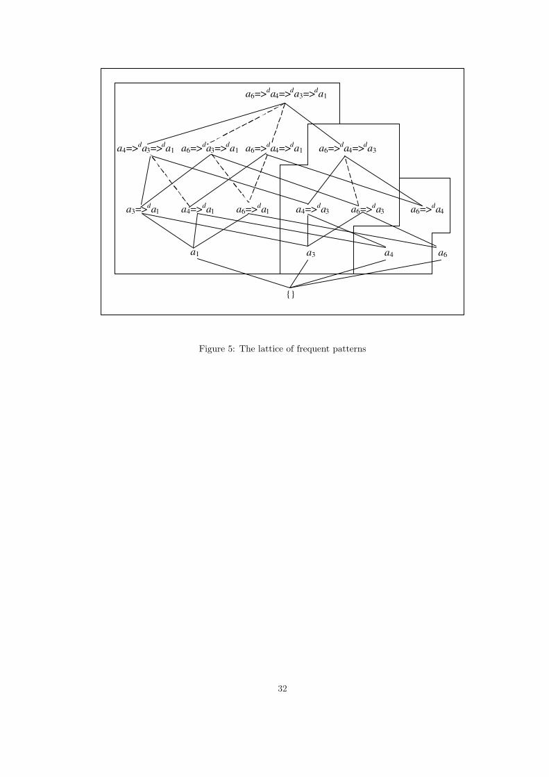
That is, in the kth iteration, for each ap∈h(β), check if both patterns α and γ, i.e., p(β,k)⇒dap
and p(α,-k)⇒dp(β,-1) respectively, are frequent. Let us consider all the DTPs as a lattice as shown in
Figure 5. And one sublattice is the set of the patterns with the same top element(e.g., a1,a3,a4, and a6).
11
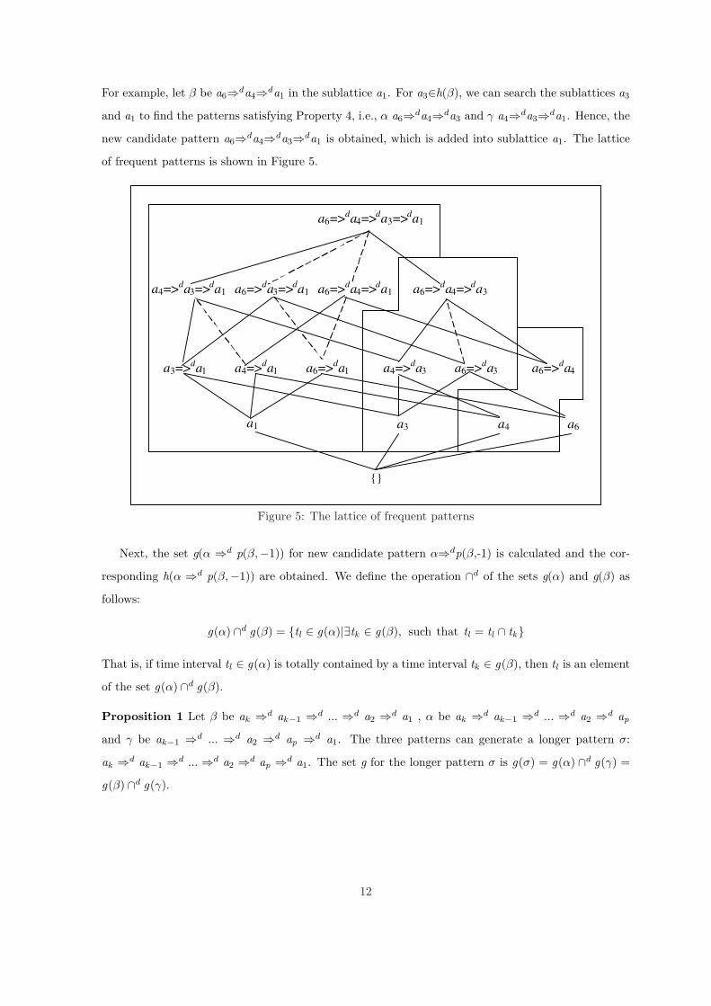
For example, let β be a6⇒da4⇒da1 in the sublattice a1. For a3∈h(β), we can search the sublattices a3
and a1 to find the patterns satisfying Property 4, i.e., α a6⇒da4⇒da3 and γ a4⇒da3⇒da1. Hence, the
new candidate pattern a6⇒da4⇒da3⇒da1 is obtained, which is added into sublattice a1. The lattice
of frequent patterns is shown in Figure 5.
a3=>da1 a4=>
da1 a6=>
da1 a4=>
da3 a6=>
da3 a6=>
da4
a4=>da3=>
da1 a6=>
da3=>
da1 a6=>
da4=>
da1 a6=>
da4=>
da3
a6=>da4=>
da3=>
da1
a1 a3 a4 a6
{}
Figure 5: The lattice of frequent patterns
Next, the set g(α ⇒d p(β,−1)) for new candidate pattern α⇒dp(β,-1) is calculated and the cor-
responding h(α ⇒d p(β,−1)) are obtained. We define the operation ∩d of the sets g(α) and g(β) as
follows:
g(α) ∩d g(β) = {tl ∈ g(α)|∃tk ∈ g(β), such that tl = tl ∩ tk}
That is, if time interval tl ∈ g(α) is totally contained by a time interval tk ∈ g(β), then tl is an element
of the set g(α) ∩d g(β).
Proposition 1 Let β be ak ⇒d ak−1 ⇒d ... ⇒d a2 ⇒d a1 , α be ak ⇒d ak−1 ⇒d ... ⇒d a2 ⇒d ap
and γ be ak−1 ⇒d ... ⇒d a2 ⇒d ap ⇒d a1. The three patterns can generate a longer pattern σ:
ak ⇒d ak−1 ⇒d ... ⇒d a2 ⇒d ap ⇒d a1. The set g for the longer pattern σ is g(σ) = g(α) ∩d g(γ) =
g(β) ∩d g(γ).
12
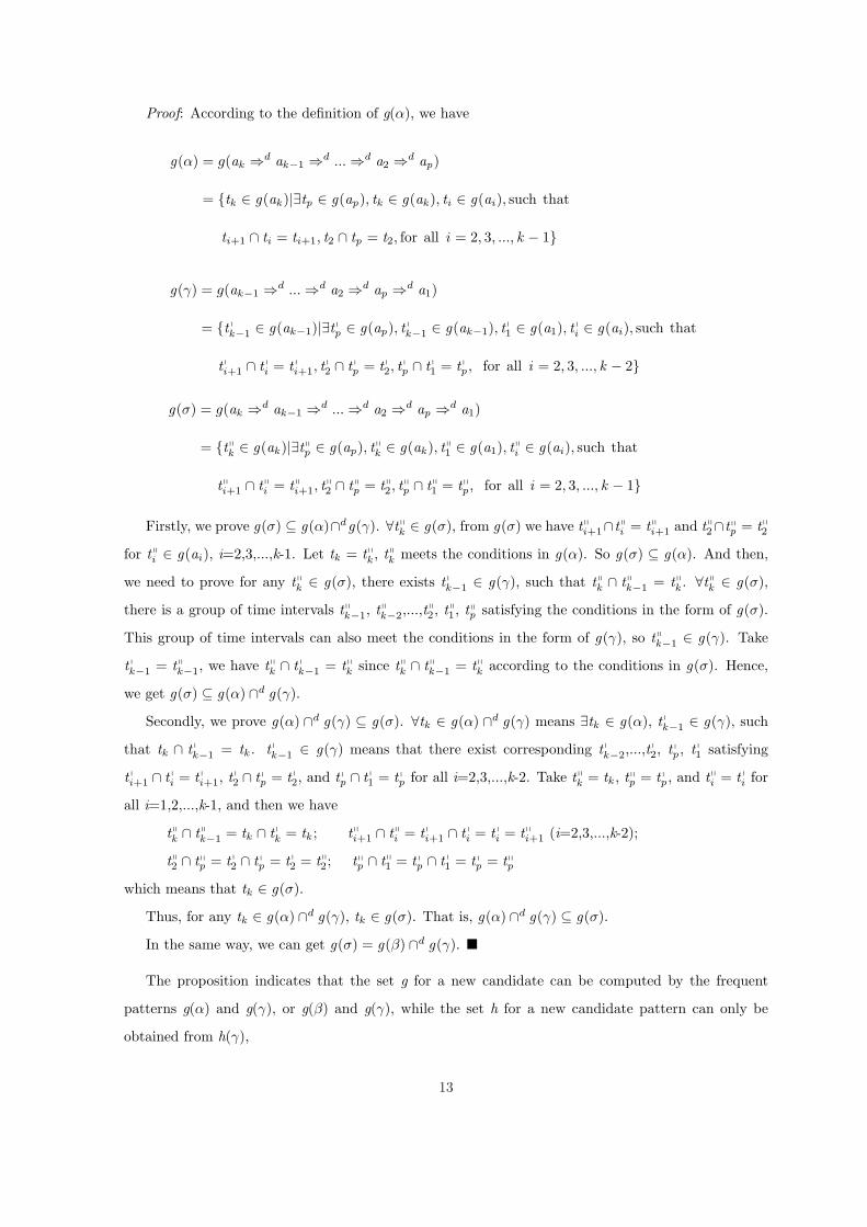
Proof: According to the definition of g(α), we have
g(α) = g(ak ⇒d ak−1 ⇒d ... ⇒d a2 ⇒d ap)
= {tk ∈ g(ak )|∃tp ∈ g(ap), tk ∈ g(ak ), ti ∈ g(ai), such that
ti+1 ∩ ti = ti+1, t2 ∩ tp = t2, for all i = 2, 3, ..., k − 1}
g(γ) = g(ak−1 ⇒d ... ⇒d a2 ⇒d ap ⇒d a1)
= {t pk−1 ∈ g(ak−1)|∃t pp ∈ g(ap), t pk−1 ∈ g(ak−1), t p1 ∈ g(a1), t pi ∈ g(ai), such that
t pi+1 ∩ t pi = t pi+1, tp2 ∩ t pp = t p2, t
pp ∩ t p1 = t pp , for all i = 2, 3, ..., k − 2}
g(σ) = g(ak ⇒d ak−1 ⇒d ... ⇒d a2 ⇒d ap ⇒d a1)
= {tqk ∈ g(ak )|∃tqp ∈ g(ap), tqk ∈ g(ak ), tq1 ∈ g(a1), tqi ∈ g(ai), such that
tqi+1 ∩ tqi = tqi+1, tq2 ∩ tqp = tq2, t
qp ∩ tq1 = tqp , for all i = 2, 3, ..., k − 1}
Firstly, we prove g(σ) ⊆ g(α)∩dg(γ). ∀tqk ∈ g(σ), from g(σ) we have tqi+1∩tqi = tqi+1 and tq2∩tqp = tq2
for tqi ∈ g(ai), i=2,3,...,k-1. Let tk = tqk , tqk meets the conditions in g(α). So g(σ) ⊆ g(α). And then,
we need to prove for any tqk ∈ g(σ), there exists t pk−1 ∈ g(γ), such that tqk ∩ tqk−1 = tqk . ∀tqk ∈ g(σ),
there is a group of time intervals tqk−1, tqk−2,...,tq2, tq1, tqp satisfying the conditions in the form of g(σ).
This group of time intervals can also meet the conditions in the form of g(γ), so tqk−1 ∈ g(γ). Take
t pk−1 = tqk−1, we have tqk ∩ t pk−1 = tqk since tqk ∩ tqk−1 = tqk according to the conditions in g(σ). Hence,
we get g(σ) ⊆ g(α) ∩d g(γ).
Secondly, we prove g(α) ∩d g(γ) ⊆ g(σ). ∀tk ∈ g(α) ∩d g(γ) means ∃tk ∈ g(α), t pk−1 ∈ g(γ), such
that tk ∩ t pk−1 = tk . t pk−1 ∈ g(γ) means that there exist corresponding t pk−2,...,tp2, t pp , t p1 satisfying
t pi+1 ∩ t pi = t pi+1, t p2 ∩ t pp = t p2, and t pp ∩ t p1 = t pp for all i=2,3,...,k-2. Take tqk = tk , tqp = t pp , and tqi = t pi for
all i=1,2,...,k-1, and then we have
tqk ∩ tqk−1 = tk ∩ t pk = tk ; tqi+1 ∩ tqi = t pi+1 ∩ t pi = t pi = tqi+1 (i=2,3,...,k-2);
tq2 ∩ tqp = t p2 ∩ t pp = t p2 = tq2; tqp ∩ tq1 = t pp ∩ t p1 = t pp = tqp
which means that tk ∈ g(σ).
Thus, for any tk ∈ g(α) ∩d g(γ), tk ∈ g(σ). That is, g(α) ∩d g(γ) ⊆ g(σ).
In the same way, we can get g(σ) = g(β) ∩d g(γ). ¥
The proposition indicates that the set g for a new candidate can be computed by the frequent
patterns g(α) and g(γ), or g(β) and g(γ), while the set h for a new candidate pattern can only be
obtained from h(γ),
13

h(α ⇒d p(β,−1)) = h(α ⇒d p(γ,−1)) = h(γ)− {ak}
Thus, we get the sets g and h for a new candidate pattern without scanning the original database and
the sets g for the single states. The procedure of join phase is shown in Figure 6.
CDTPk .Gen()1. for all pattern β∈FDTPk−1 do2. for all aj∈h(β) do3. for α∈FDTPk−1,p(α,-1)=aj do4. if Property 4 is satisfied then
5. CDTPk=CDTPk
S{α⇒dp(β,-1)}6. end if7. end for8. end for9. end for
Figure 6: The procedure used for CDTPk
(3). Pruning phase
In this phase, if the support degree of a candidate pattern in CDTPk is smaller than the user-
specified threshold, then prune it from CDTPk . At last, FDTPk is obtained. Intercross Step 2 and
Step 3 until Property 2 cannot be satisfied any longer. The procedure of pruning phase is shown in
Figure 7.
FDTPk .Gen()1. FDTP0 known, FDTPk=∅ (k=1,2,...)2. for (k=1;FDTPk−1 6=∅;k++) do3. CDTPk=CDTPk .Gen(FDTPk−1);4. for all candidate patterns β∈CDTPk do5. FDTPk={β∈CDTPk ||g(β)|≥minsupport}6. end for7.end for8. FDTP=
SkFDTPk
Figure 7: The procedure used for FDTPk
(4). Generating valid DTPs
Given a pattern α: ak ⇒d ak−1 ⇒d ... ⇒d a2 ⇒d a1, it is necessary to know how frequent α is
when a1 has occurred, when a2 ⇒d a1 has occurred, when a3 ⇒d a2 ⇒d a1 has occurred, and so on.
Thus, we can get the pattern β⇒dγ as mentioned in Section 3,
(ak ⇒d ak−1 ⇒d ... ⇒d aj+1) ⇒d (aj ⇒d aj−1 ⇒d ... ⇒d a2 ⇒d a1) (1 ≤ j ≤ k − 1)
That is, a frequent pattern can generate (k-1) valid DTPs at most. Calculating the confidence degree
starting from the longest consequent pattern, i.e., from the pattern with j=k-1, the patterns meeting the
confidence threshold will be valid DTPs. The pattern α will be stopped to compute if confidence(β⇒dγ)
14
is less than the threshold. Otherwise, the confidence degree of a shorter consequent pattern, i.e., j=j-1,
is computed next.
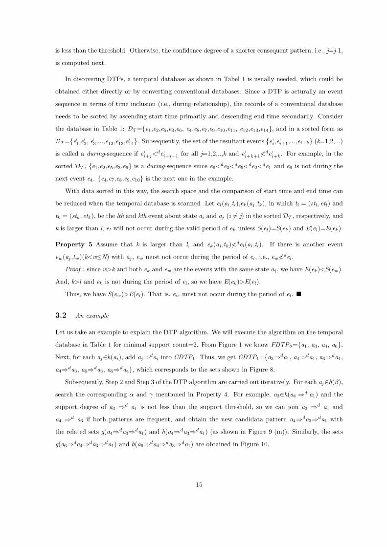
In discovering DTPs, a temporal database as shown in Tabel 1 is usually needed, which could be
obtained either directly or by converting conventional databases. Since a DTP is acturally an event
sequence in terms of time inclusion (i.e., during relationship), the records of a conventional database
needs to be sorted by ascending start time primarily and descending end time secondarily. Consider
the database in Table 1: DT ={e1,e2,e5,e3,e6, e4,e8,e7,e9,e10,e11, e12,e13,e14}, and in a sorted form as
DT ={ep1,ep2, ep3,...,ep12,e
p13,e
p14}. Subsequently, the set of the resultant events {e pi ,e pi+1,...,ei+k} (k=1,2,...)
is called a during-sequence if e pi+j<de pi+j−1 for all j=1,2,..,k and e pi+k+1≮de pi+k . For example, in the
sorted DT , {e1,e2,e5,e3,e6} is a during-sequence since e6<de3<
de5<de2<
de1 and e6 is not during the
next event e4. {e4,e7,e8,e9,e10} is the next one in the example.
With data sorted in this way, the search space and the comparison of start time and end time can
be reduced when the temporal database is scanned. Let el(ai ,tl),ek (aj ,tk ), in which tl = (stl , etl) and
tk = (stk , etk ), be the lth and kth event about state ai and aj (i 6= j) in the sorted DT , respectively, and
k is larger than l, el will not occur during the valid period of ek unless S(el)=S(ek ) and E(el)=E(ek ).
Property 5 Assume that k is larger than l, and ek (aj ,tk )≮del(ai ,tl). If there is another event
ew (aj ,tw )(k<w≤N) with aj , ew must not occur during the period of el , i.e., ew≮del .
Proof : since w>k and both ek and ew are the events with the same state aj , we have E(ek )<S(ew ).
And, k>l and ek is not during the period of el , so we have E(ek )>E(el).
Thus, we have S(ew )>E(el). That is, ew must not occur during the period of el . ¥
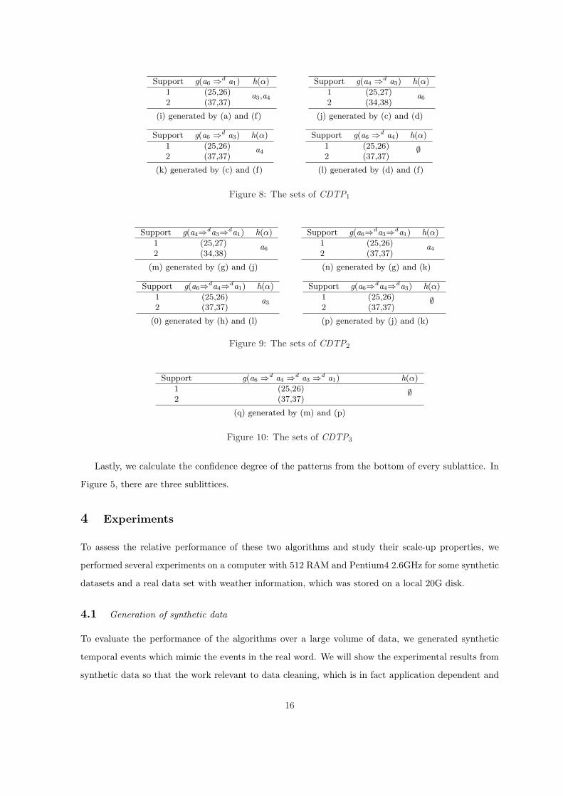
3.2 An example
Let us take an example to explain the DTP algorithm. We will execute the algorithm on the temporal
database in Table 1 for minimal support count=2. From Figure 1 we know FDTP0={a1, a3, a4, a6}.Next, for each aj∈h(ai), add aj⇒dai into CDTP1. Thus, we get CDTP1={a3⇒da1, a4⇒da1, a6⇒da1,
a4⇒da3, a6⇒da3, a6⇒da4}, which corresponds to the sets shown in Figure 8.
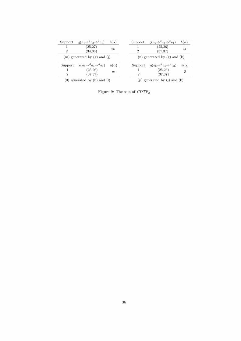
Subsequently, Step 2 and Step 3 of the DTP algorithm are carried out iteratively. For each aj∈h(β),
search the corresponding α and γ mentioned in Property 4. For example, a3∈h(a4 ⇒d a1) and the
support degree of a3 ⇒d a1 is not less than the support threshold, so we can join a3 ⇒d a1 and
a4 ⇒d a3 if both patterns are frequent, and obtain the new candidata pattern a4⇒da3⇒da1 with
the related sets g(a4⇒da3⇒da1) and h(a4⇒da3⇒da1) (as shown in Figure 9 (m)). Similarly, the sets
g(a6⇒da4⇒da3⇒da1) and h(a6⇒da4⇒da3⇒da1) are obtained in Figure 10.
15
Support g(a6 ⇒d a1) h(α)
1 (25,26)2 (37,37)
a3,a4
Support g(a4 ⇒d a3) h(α)
1 (25,27)2 (34,38)
a6
(i) generated by (a) and (f) (j) generated by (c) and (d)
Support g(a6 ⇒d a3) h(α)
1 (25,26)2 (37,37)
a4
Support g(a6 ⇒d a4) h(α)
1 (25,26)2 (37,37)
∅
(k) generated by (c) and (f) (l) generated by (d) and (f)
Figure 8: The sets of CDTP1
Support g(a4⇒da3⇒da1) h(α)
1 (25,27)2 (34,38)
a6
Support g(a6⇒da3⇒da1) h(α)
1 (25,26)2 (37,37)
a4
(m) generated by (g) and (j) (n) generated by (g) and (k)
Support g(a6⇒da4⇒da1) h(α)
1 (25,26)2 (37,37)
a3
Support g(a6⇒da4⇒da3) h(α)
1 (25,26)2 (37,37)
∅
(0) generated by (h) and (l) (p) generated by (j) and (k)
Figure 9: The sets of CDTP2
Support g(a6 ⇒d a4 ⇒d a3 ⇒d a1) h(α)
1 (25,26)2 (37,37)
∅
(q) generated by (m) and (p)
Figure 10: The sets of CDTP3
Lastly, we calculate the confidence degree of the patterns from the bottom of every sublattice. In
Figure 5, there are three sublittices.
4 Experiments
To assess the relative performance of these two algorithms and study their scale-up properties, we
performed several experiments on a computer with 512 RAM and Pentium4 2.6GHz for some synthetic
datasets and a real data set with weather information, which was stored on a local 20G disk.
4.1 Generation of synthetic data
To evaluate the performance of the algorithms over a large volume of data, we generated synthetic
temporal events which mimic the events in the real word. We will show the experimental results from
synthetic data so that the work relevant to data cleaning, which is in fact application dependent and
16
also orthogonal to the incremental technique proposed, is hence omitted for simplicity. For obtaining
reliable experimental results, the method to generate synthetic data we employed in this study is
similar to the ones used in [12].
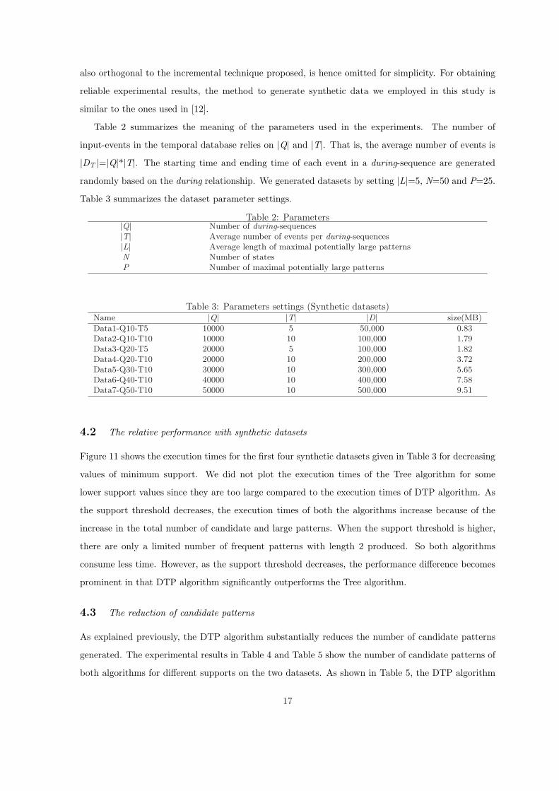
Table 2 summarizes the meaning of the parameters used in the experiments. The number of
input-events in the temporal database relies on |Q| and |T|. That is, the average number of events is
|DT |=|Q|*|T|. The starting time and ending time of each event in a during-sequence are generated
randomly based on the during relationship. We generated datasets by setting |L|=5, N=50 and P=25.
Table 3 summarizes the dataset parameter settings.
Table 2: Parameters|Q| Number of during-sequences|T| Average number of events per during-sequences|L| Average length of maximal potentially large patternsN Number of statesP Number of maximal potentially large patterns
Table 3: Parameters settings (Synthetic datasets)Name |Q| |T| |D| size(MB)
Data1-Q10-T5 10000 5 50,000 0.83Data2-Q10-T10 10000 10 100,000 1.79Data3-Q20-T5 20000 5 100,000 1.82Data4-Q20-T10 20000 10 200,000 3.72Data5-Q30-T10 30000 10 300,000 5.65Data6-Q40-T10 40000 10 400,000 7.58Data7-Q50-T10 50000 10 500,000 9.51
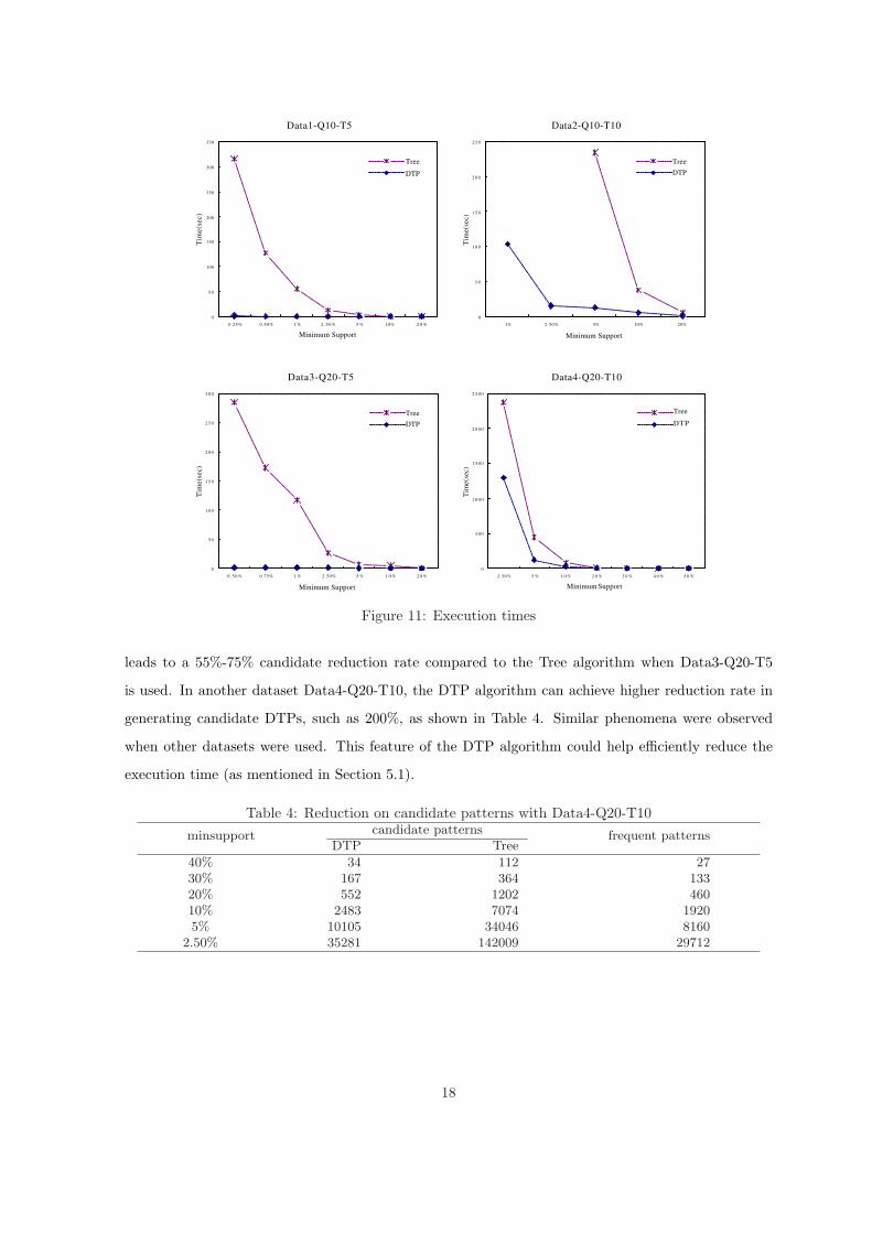
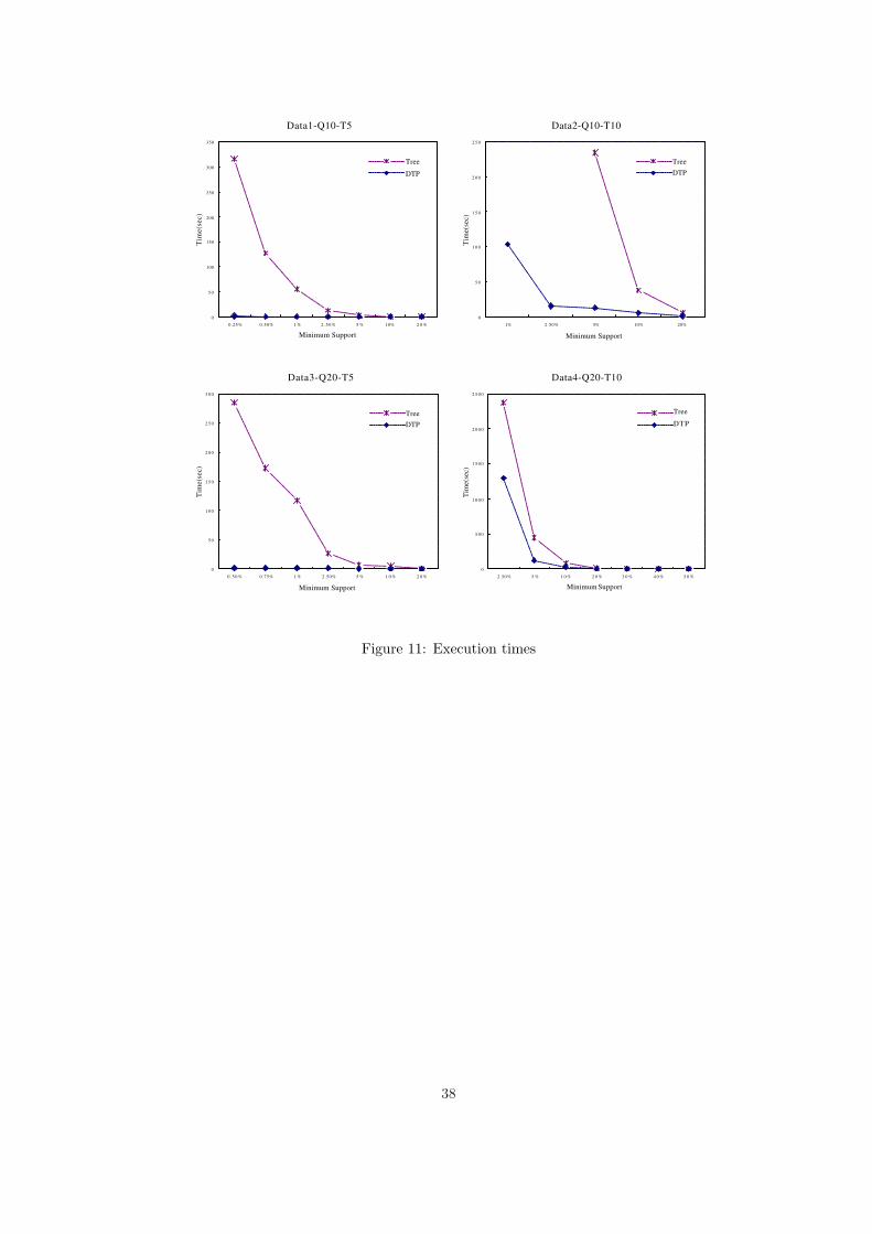
4.2 The relative performance with synthetic datasets
Figure 11 shows the execution times for the first four synthetic datasets given in Table 3 for decreasing
values of minimum support. We did not plot the execution times of the Tree algorithm for some
lower support values since they are too large compared to the execution times of DTP algorithm. As
the support threshold decreases, the execution times of both the algorithms increase because of the
increase in the total number of candidate and large patterns. When the support threshold is higher,
there are only a limited number of frequent patterns with length 2 produced. So both algorithms
consume less time. However, as the support threshold decreases, the performance difference becomes
prominent in that DTP algorithm significantly outperforms the Tree algorithm.
4.3 The reduction of candidate patterns
As explained previously, the DTP algorithm substantially reduces the number of candidate patterns
generated. The experimental results in Table 4 and Table 5 show the number of candidate patterns of
both algorithms for different supports on the two datasets. As shown in Table 5, the DTP algorithm
17
Data1-Q10-T5
0
5 0
100
150
200
250
300
350
0.25% 0.50% 1 % 2 . 5 0 % 5 % 10% 2 0 %
Minimum Support
Tim
e(s
ec)
Tree
DTP
Data2-Q10-T10
0
5 0
1 0 0
1 5 0
2 0 0
2 5 0
1% 2.50% 5% 10% 20%
Minimum Support
Tim
e(s
ec)
Tree
DTP
Data3-Q20-T5
0
5 0
1 0 0
1 5 0
2 0 0
2 5 0
3 0 0
0 . 5 0 % 0.75% 1 % 2.50% 5 % 1 0 % 2 0 %
Minimum Support
Tim
e(s
ec)
Tree
DTP
Data4-Q20-T10
0
5 0 0
1 0 0 0
1 5 0 0
2 0 0 0
2 5 0 0
2.50% 5 % 1 0 % 2 0 % 3 0 % 4 0 % 5 0 %
Minimum Support
Tim
e(se
c)
Tree
DTP
Figure 11: Execution times
leads to a 55%-75% candidate reduction rate compared to the Tree algorithm when Data3-Q20-T5
is used. In another dataset Data4-Q20-T10, the DTP algorithm can achieve higher reduction rate in
generating candidate DTPs, such as 200%, as shown in Table 4. Similar phenomena were observed
when other datasets were used. This feature of the DTP algorithm could help efficiently reduce the
execution time (as mentioned in Section 5.1).
Table 4: Reduction on candidate patterns with Data4-Q20-T10candidate patternsminsupport
DTP Treefrequent patterns
40% 34 112 2730% 167 364 13320% 552 1202 46010% 2483 7074 19205% 10105 34046 8160
2.50% 35281 142009 29712
18
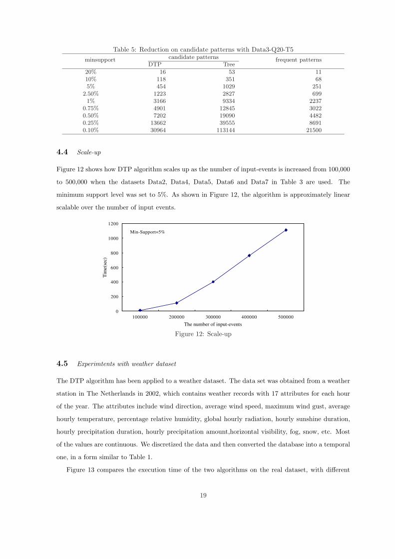
Table 5: Reduction on candidate patterns with Data3-Q20-T5candidate patternsminsupport
DTP Treefrequent patterns
20% 16 53 1110% 118 351 685% 454 1029 251
2.50% 1223 2827 6991% 3166 9334 2237
0.75% 4901 12845 30220.50% 7202 19090 44820.25% 13662 39555 86910.10% 30964 113144 21500
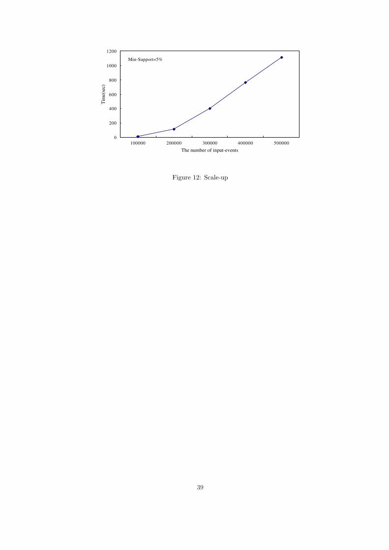
4.4 Scale-up
Figure 12 shows how DTP algorithm scales up as the number of input-events is increased from 100,000
to 500,000 when the datasets Data2, Data4, Data5, Data6 and Data7 in Table 3 are used. The
minimum support level was set to 5%. As shown in Figure 12, the algorithm is approximately linear
scalable over the number of input events.
Min-Support=5%
0
200
400
600
800
1000
1200
100000 200000 300000 400000 500000
The number of input-events
Tim
e(se
c)
Figure 12: Scale-up
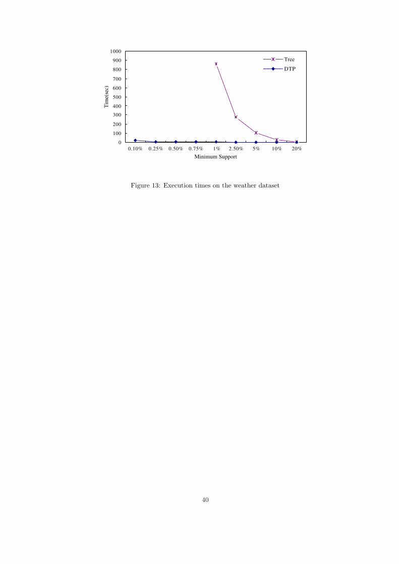
4.5 Experimtents with weather dataset
The DTP algorithm has been applied to a weather dataset. The data set was obtained from a weather
station in The Netherlands in 2002, which contains weather records with 17 attributes for each hour
of the year. The attributes include wind direction, average wind speed, maximum wind gust, average
hourly temperature, percentage relative humidity, global hourly radiation, hourly sunshine duration,
hourly precipitation duration, hourly precipitation amount,horizontal visibility, fog, snow, etc. Most
of the values are continuous. We discretized the data and then converted the database into a temporal
one, in a form similar to Table 1.
Figure 13 compares the execution time of the two algorithms on the real dataset, with different
19
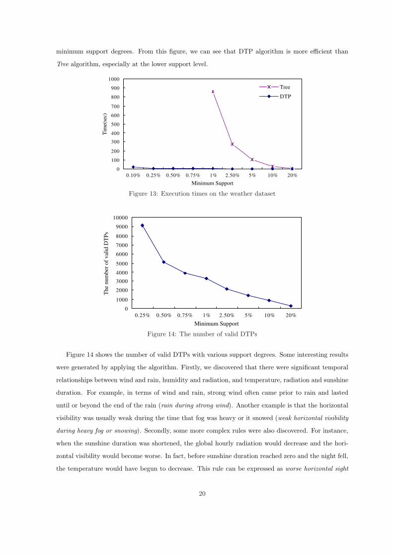
minimum support degrees. From this figure, we can see that DTP algorithm is more efficient than
Tree algorithm, especially at the lower support level.
0
100
200
300
400
500
600
700
800
900
1000
0.10% 0.25% 0.50% 0.75% 1% 2.50% 5% 10% 20%
Minimum Support
Tim
e(se
c)
Tree
DTP
Figure 13: Execution times on the weather dataset
0
1000
2000
3000
4000
5000
6000
7000
8000
9000
10000
0.25% 0.50% 0.75% 1% 2.50% 5% 10% 20%
Minimum Support
The
num
ber
of
val
id D
TP
s
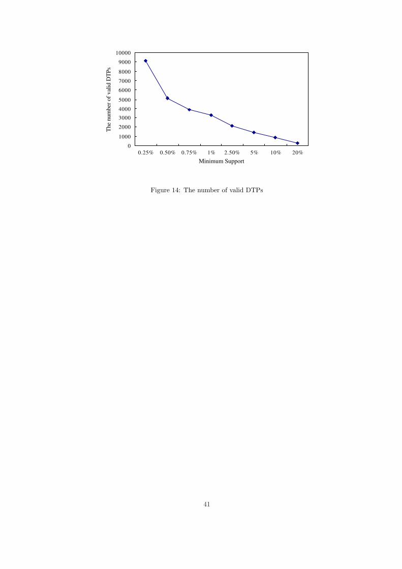
Figure 14: The number of valid DTPs
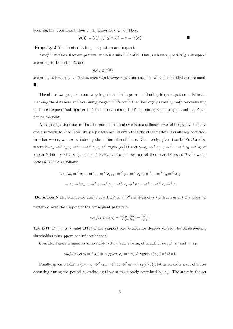
Figure 14 shows the number of valid DTPs with various support degrees. Some interesting results
were generated by applying the algorithm. Firstly, we discovered that there were significant temporal
relationships between wind and rain, humidity and radiation, and temperature, radiation and sunshine
duration. For example, in terms of wind and rain, strong wind often came prior to rain and lasted
until or beyond the end of the rain (rain during strong wind). Another example is that the horizontal
visibility was usually weak during the time that fog was heavy or it snowed (weak horizontal visibility
during heavy fog or snowing). Secondly, some more complex rules were also discovered. For instance,
when the sunshine duration was shortened, the global hourly radiation would decrease and the hori-
zontal visibility would become worse. In fact, before sunshine duration reached zero and the night fell,
the temperature would have begun to decrease. This rule can be expressed as worse horizontal sight
20

during no global hourly radiation during no sunshine during very lower temperature.
5 Conclusions and future work
In this paper, we have studied the problem of discovering during-temporal patterns between events
and proposed the DTP algorithm. By analyzing the properties of the during relationship, we have
developed an optimization technique with pruning strategies that enabled us to retrieve the patterns
with minimal database scan. The experimental results have illustrated the effectiveness and efficiency
of the algorithm. An ongoing effort centers on extending this algorithm to discovering the dynamic
temporal database, since in the light of the fact that the content of a TDB always keeps growing
and the discovered patterns need to be maintained periodically over time. While there are some
studies on mining of dynamic database and maintenance of association rules [1,2,4,5,15], our focus is
on the maintenance of temporal patterns, so as to reduce the overhead of rediscovering patterns in the
presence of data updates.
References
[1] A. Veloso, W. Meira Jr., M.B.De Carvalho, S.Parthasarathy, and M.Zaki. (2003). Parallel, Incre-
mental and Interactive Mining for Frequent Itemsets in Evolving Databases. In Proceedings of
the Sixth SIAM Workshop on High Performance Data Mining, May 2003.
[2] C. Jin, W. Qian, C. Sha, J. Yu, and A. Zhou. (2003). Dynamically Maintaining Frequent Items over
A Data Stream. In Proceedings of the 12th ACM CIKM International Conference on Information
and Knowledge Management, pages 287–294, 2003.
[3] Chris P.Rainsford, and John F.Roddic. (1999). Adding Temporal Semantics to Association Rules.
In Proc. of the 3rd European conf. on principles and practice of knowledge discovery in databases,
pages 504-509, 1999.
[4] D.W.Cheung, J.Han, V.T.Ng, and C.Y.Wong. (1996). Maintenance of Discovered Association
Rules in Large Databases: An Incremental Updating Technique. Proc, Int’l Conf. Data Eng.,
(ICDE’96)S.Y.W.Su,ed., pp.106-114,1996.
[5] D.W.Cheung, S.D.Lee, and B.Kao. (1997). A General Incremental Technique for Maintaining Dis-
covered Association Rules. In Proc. Fifth Int’l Conf. Database Systems for Advanced Applications,
1997.
21
[6] F.Hoppner. (2001). Discovery of Temporal Patterns—Learning Rules about the Qualitative Be-
haviour of Time Series. In PKDD’01, number 2168 of LNAI, Freiburg, Germany, pages 192-203,
2001.
[7] Guoqing Chen, Jiang Ai, Wei Yu. (2002) Discovering Temporal Association Rules for Time-Lag
Data. Proceedings of International Conference on E-Business (ICEB2002), Beijing, May 2002.
[8] G.Das, K.I.Lin, H. Mannila. (1998). Rule discovery from time series. In Proceedings of the inter-
national conference on KDD and Data Mining, 1998.
[9] J. Chang and W. Lee. (2003). Finding Recent Frequent Itemsets Adaptively over Online Data
Streams. In Proceedings of the 9th ACM SIGKDD International Conference on Knowledge Dis-
covery and Data Mining, pages 487–492, 2003.
[10] James F.Allen. (1983). Maintaining Knowledge about Temporal Intervals. Communication of the
ACM, Volume 26, Number 11, P832-843, November 1983.
[11] Mohammed.J.ZAKI. (2000). SPADE: An Efficient Algorithm for Mining Frequent Sequences.
Machine Learning, 0, 1-31, 2000.
[12] R.Agrawal, and R.Srikant. (1994). Fast algorithm for mining association rules. In Proc. of the
20th Int’l Conference on Very Large Databases, Santiago, Chile, September, 1994.
[13] R.Agrawal, and R.Srikant. (1995). Mining Sequential Patterns. International Conference on Data
Engineering(ICDE), March, Taiwan, 1995.
[14] R.Agrawal, T.Imielinski, and A.Swami. (1993). Mining association rules between sets of items in
large databases. In Proceedings of the 1993 ACM SIGMOD International Conference on Manage-
ment of Data, pages 207-216, Washington DC, May 26-28, 1993. 10.
[15] Y.Chi, H.J.Wang, Philip S.Yu, and Richard R. Muntz. (2004). Catch the Moment Maintaining
Closed Frequent Itemsets. http://citeseer.ist.psu.edu.
22

Table 1: A Temporal DatabaseEvent State Starting Time Ending Time
e1 a1 1 20e2 a3 1 4e3 a4 5 7e4 a1 22 28e5 a2 2 8e6 a3 10 13e7 a5 25 35e8 a3 23 28e9 a4 25 27e10 a6 25 26e11 a1 30 40e12 a3 30 38e13 a4 34 38e14 a6 37 37
23

Table 2: Parameters|Q| Number of during-sequences|T| Average number of events per during-sequences|L| Average length of maximal potentially large patternsN Number of statesP Number of maximal potentially large patterns
24
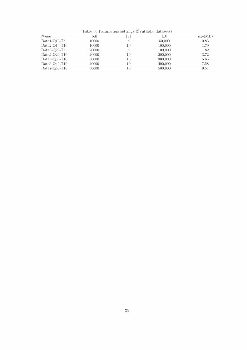
Table 3: Parameters settings (Synthetic datasets)Name |Q| |T| |D| size(MB)
Data1-Q10-T5 10000 5 50,000 0.83Data2-Q10-T10 10000 10 100,000 1.79Data3-Q20-T5 20000 5 100,000 1.82Data4-Q20-T10 20000 10 200,000 3.72Data5-Q30-T10 30000 10 300,000 5.65Data6-Q40-T10 40000 10 400,000 7.58Data7-Q50-T10 50000 10 500,000 9.51
25
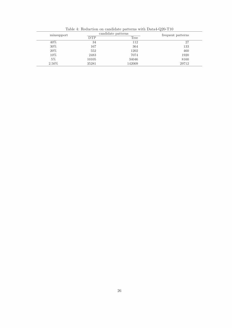
Table 4: Reduction on candidate patterns with Data4-Q20-T10candidate patternsminsupport
DTP Treefrequent patterns
40% 34 112 2730% 167 364 13320% 552 1202 46010% 2483 7074 19205% 10105 34046 8160
2.50% 35281 142009 29712
26

Table 5: Reduction on candidate patterns with Data3-Q20-T5candidate patternsminsupport
DTP Treefrequent patterns
20% 16 53 1110% 118 351 685% 454 1029 251
2.50% 1223 2827 6991% 3166 9334 2237
0.75% 4901 12845 30220.50% 7202 19090 44820.25% 13662 39555 86910.10% 30964 113144 21500
27
Support g(a1) h(a1)
1 (1,20)2 (22,28) a2,a3,a4,a6
3 (30,40)
Support g(a2) h(a2)
1 (2,8) a4
Support g(a3) h(a3)
1 (1,4)2 (10,13)3 (23,28)
a4,a6
4 (30,38)
(a) (b) (c)
Support g(a4) h(a4)
1 (5,7)2 (25,27) a6
3 (34,38)
Support g(a5) h(a5)
1 (25,35) a4,a6
Support g(a6) h(a6)
1 (25,26)2 (37,37)
∅
(d) (e) (f)
Support g(a3 ⇒d a1) h(α)
1 (1,4)(10,13)
2 (23,28)a4,a6
3 (30,38)
Support g(a4 ⇒d a1) h(α)
1 (5,7)2 (25,27) a3,a6
3 (34,38)
(g) (h)
Figure 1: The examples of the sets g and h
28
t
a3
a2 a2
a1
a3
a2
Figure 2: A counterexample for pattern transitivity
29
a2
a5 a6 a9 a10 a11 a12
a6
a5
a4
a2 a7 a9 a10 a11 a12
a11
a5 a6 a7 a9 a12 a13
Figure 3: trees of frequent DTP1
30

FDTP0.Gen()1. FDTP0=∅;2. for all ai∈A do3. if |g(ai)|≥ minsupport then4. FDTP0=FDTP0∪{ai};5. end if6. end for
Figure 4: The procedure used for FDTP0
31
a3=>da1 a4=>
da1 a6=>
da1 a4=>
da3 a6=>
da3 a6=>
da4
a4=>da3=>
da1 a6=>
da3=>
da1 a6=>
da4=>
da1 a6=>
da4=>
da3
a6=>da4=>
da3=>
da1
a1 a3 a4 a6
{}
Figure 5: The lattice of frequent patterns
32

CDTPk .Gen()1. for all pattern β∈FDTPk−1 do2. for all aj∈h(β) do3. for α∈FDTPk−1,p(α,-1)=aj do4. if Property 4 is satisfied then
5. CDTPk=CDTPk
S{α⇒dp(β,-1)}6. end if7. end for8. end for9. end for
Figure 6: The procedure used for CDTPk
33

FDTPk .Gen()1. FDTP0 known, FDTPk=∅ (k=1,2,...)2. for (k=1;FDTPk−1 6=∅;k++) do3. CDTPk=CDTPk .Gen(FDTPk−1);4. for all candidate patterns β∈CDTPk do5. FDTPk={β∈CDTPk ||g(β)|≥minsupport}6. end for7.end for8. FDTP=
SkFDTPk
Figure 7: The procedure used for FDTPk
34

Support g(a6 ⇒d a1) h(α)
1 (25,26)2 (37,37)
a3,a4
Support g(a4 ⇒d a3) h(α)
1 (25,27)2 (34,38)
a6
(i) generated by (a) and (f) (j) generated by (c) and (d)
Support g(a6 ⇒d a3) h(α)
1 (25,26)2 (37,37)
a4
Support g(a6 ⇒d a4) h(α)
1 (25,26)2 (37,37)
∅
(k) generated by (c) and (f) (l) generated by (d) and (f)
Figure 8: The sets of CDTP1
35
Support g(a4⇒da3⇒da1) h(α)
1 (25,27)2 (34,38)
a6
Support g(a6⇒da3⇒da1) h(α)
1 (25,26)2 (37,37)
a4
(m) generated by (g) and (j) (n) generated by (g) and (k)
Support g(a6⇒da4⇒da1) h(α)
1 (25,26)2 (37,37)
a3
Support g(a6⇒da4⇒da3) h(α)
1 (25,26)2 (37,37)
∅
(0) generated by (h) and (l) (p) generated by (j) and (k)
Figure 9: The sets of CDTP2
36

Support g(a6 ⇒d a4 ⇒d a3 ⇒d a1) h(α)
1 (25,26)2 (37,37)
∅
(q) generated by (m) and (p)
Figure 10: The sets of CDTP3
37
Data1-Q10-T5
0
5 0
100
150
200
250
300
350
0.25% 0.50% 1 % 2 . 5 0 % 5 % 10% 2 0 %
Minimum Support
Tim
e(s
ec)
Tree
DTP
Data2-Q10-T10
0
5 0
1 0 0
1 5 0
2 0 0
2 5 0
1% 2.50% 5% 10% 20%
Minimum Support
Tim
e(s
ec)
Tree
DTP
Data3-Q20-T5
0
5 0
1 0 0
1 5 0
2 0 0
2 5 0
3 0 0
0 . 5 0 % 0.75% 1 % 2.50% 5 % 1 0 % 2 0 %
Minimum Support
Tim
e(s
ec)
Tree
DTP
Data4-Q20-T10
0
5 0 0
1 0 0 0
1 5 0 0
2 0 0 0
2 5 0 0
2.50% 5 % 1 0 % 2 0 % 3 0 % 4 0 % 5 0 %
Minimum Support
Tim
e(se
c)
Tree
DTP
Figure 11: Execution times
38
Min-Support=5%
0
200
400
600
800
1000
1200
100000 200000 300000 400000 500000
The number of input-events
Tim
e(se
c)
Figure 12: Scale-up
39
0
100
200
300
400
500
600
700
800
900
1000
0.10% 0.25% 0.50% 0.75% 1% 2.50% 5% 10% 20%
Minimum Support
Tim
e(se
c)
Tree
DTP
Figure 13: Execution times on the weather dataset
40
0
1000
2000
3000
4000
5000
6000
7000
8000
9000
10000
0.25% 0.50% 0.75% 1% 2.50% 5% 10% 20%
Minimum Support
The
num
ber
of
val
id D
TP
s
Figure 14: The number of valid DTPs
41