Discovering Exotic Mesons @CLAS12

Discovering Exotic Mesons @CLAS12

CLAS collaboration meeting JLab, March 2019

Vincent MATHIEU

Jefferson LabJoint Physics Analysis Center

Joint Physics Analysis Center

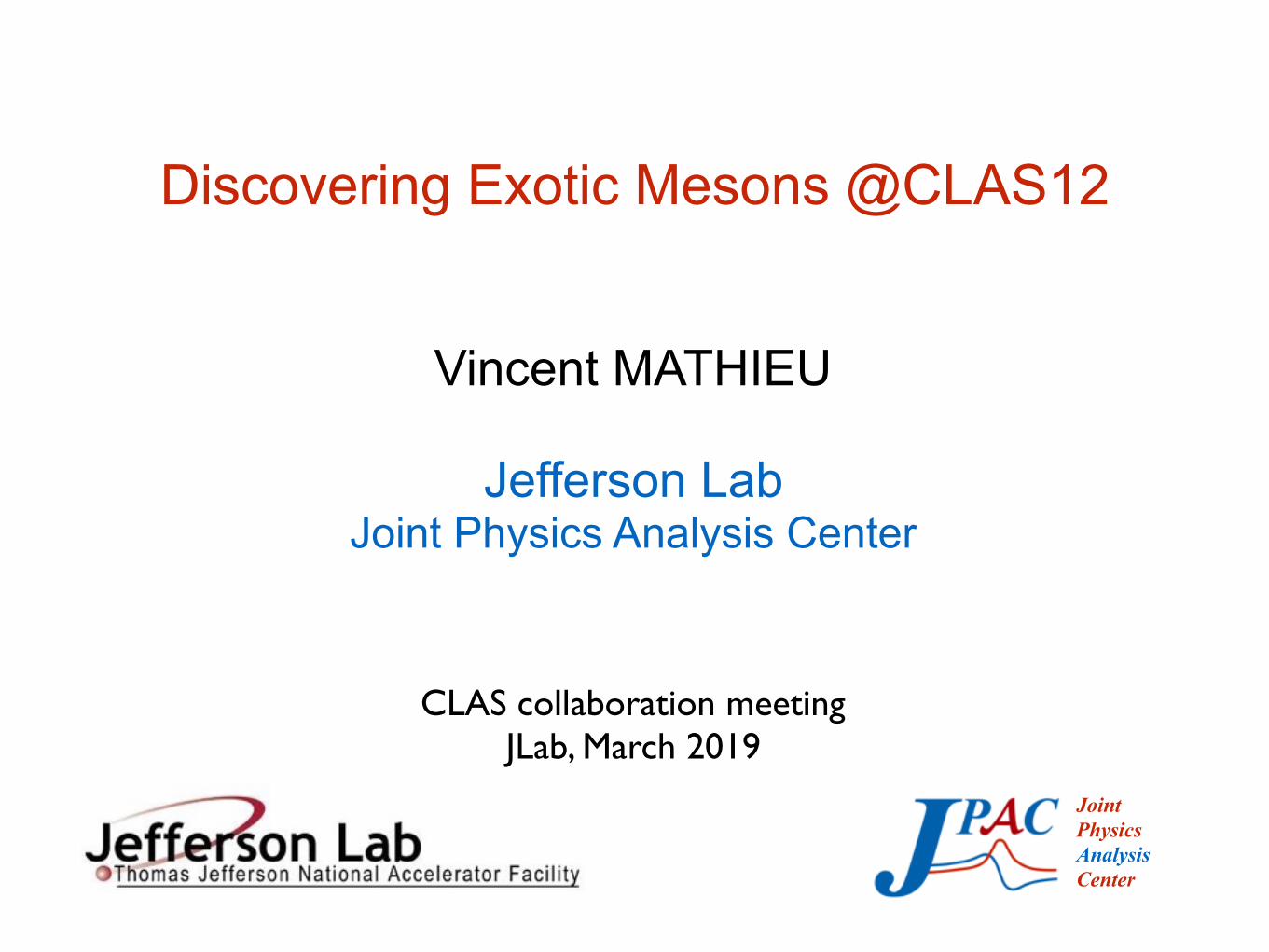
2Ordinary and Exotic HadronsOrdinary baryons:

Ordinary mesons

protonneutron

pion

baryon ⇤

⌧ ⇠ 103s stable

⌧ ⇠ 10�10s

⌧ ⇠ 10�8sCC

kaon⌧ ⇠ 10�8s

⌧ ⇠ 10�20s

J/

Exotic matterglueballshybrid mesons

tetraquarks pentaquarks

CD

UC

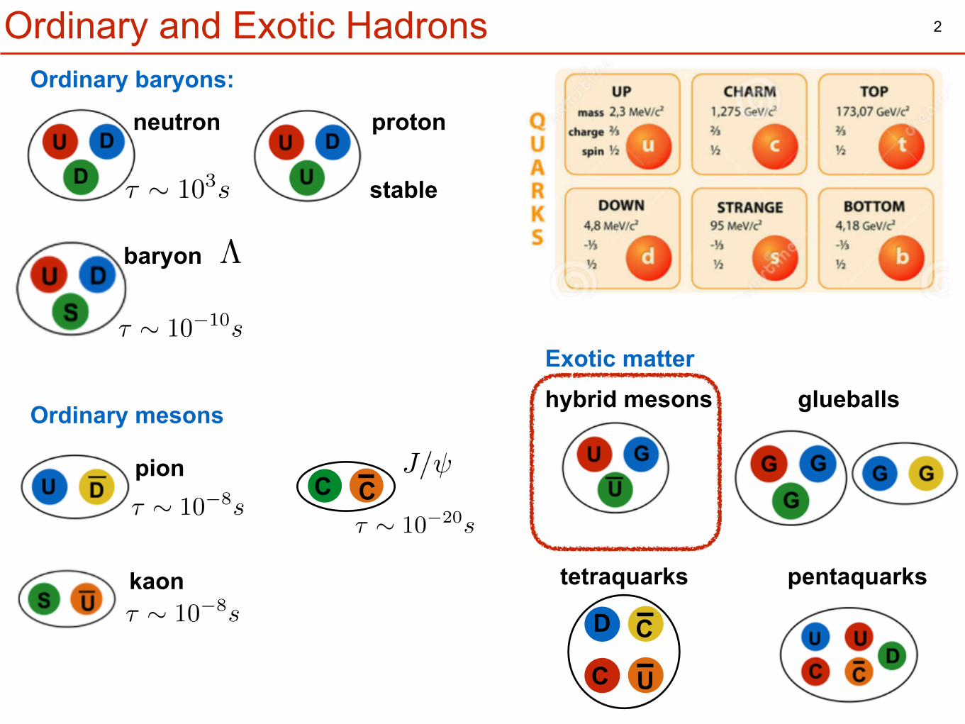
3Hybrid Mesons Production

hybrid mesons

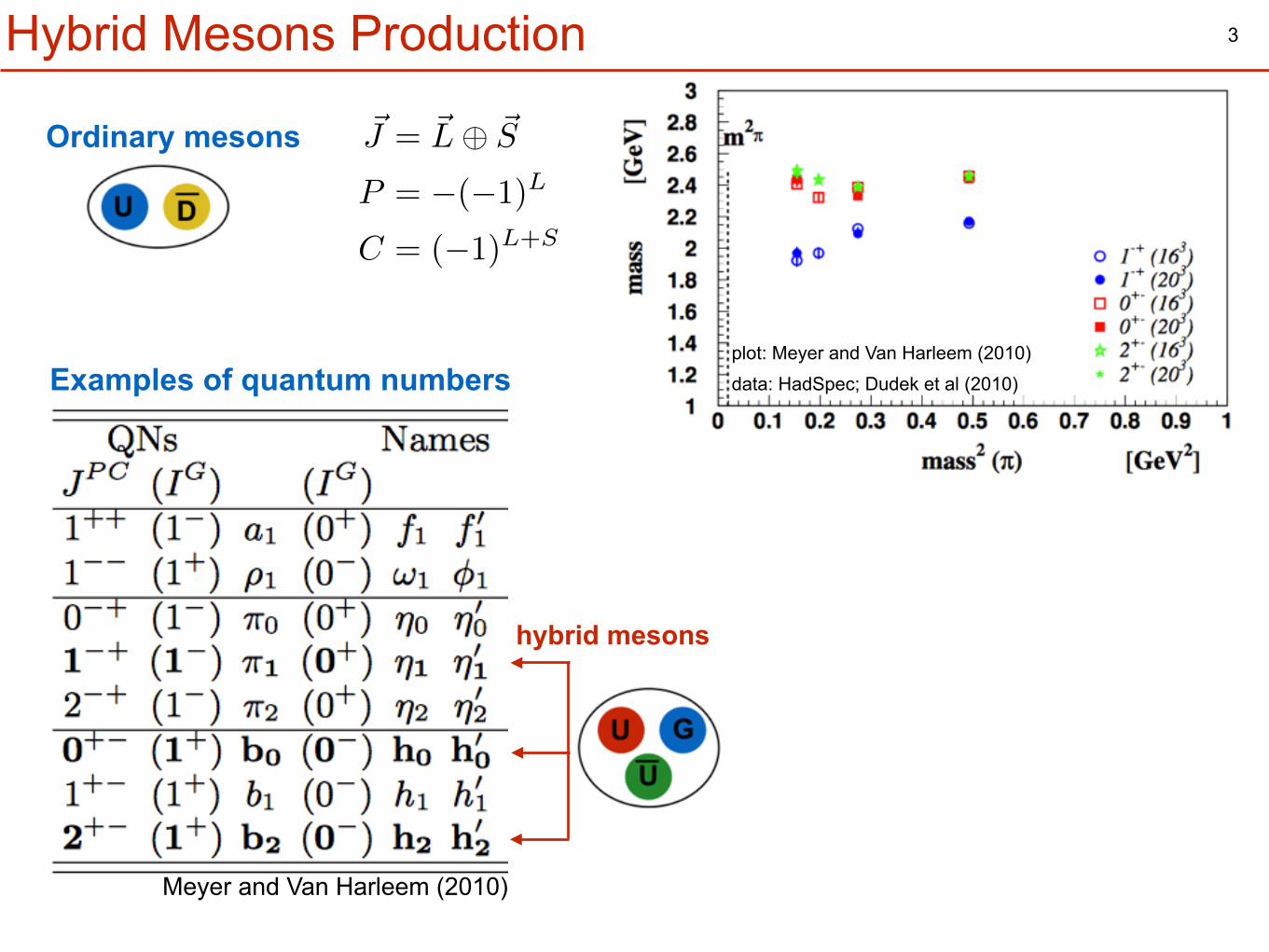
Ordinary mesons ~J = ~L� ~S

P = �(�1)L

C = (�1)L+S

Meyer and Van Harleem (2010)

Examples of quantum numbers


hybrid mesons


P = �(�1)L

C = (�1)L+S


Examples of quantum numbersplot: Meyer and Van Harleem (2010)

data: HadSpec; Dudek et al (2010)


hybrid mesons


P = �(�1)L

C = (�1)L+S


Examples of quantum numbersplot: Meyer and Van Harleem (2010)

data: HadSpec; Dudek et al (2010)

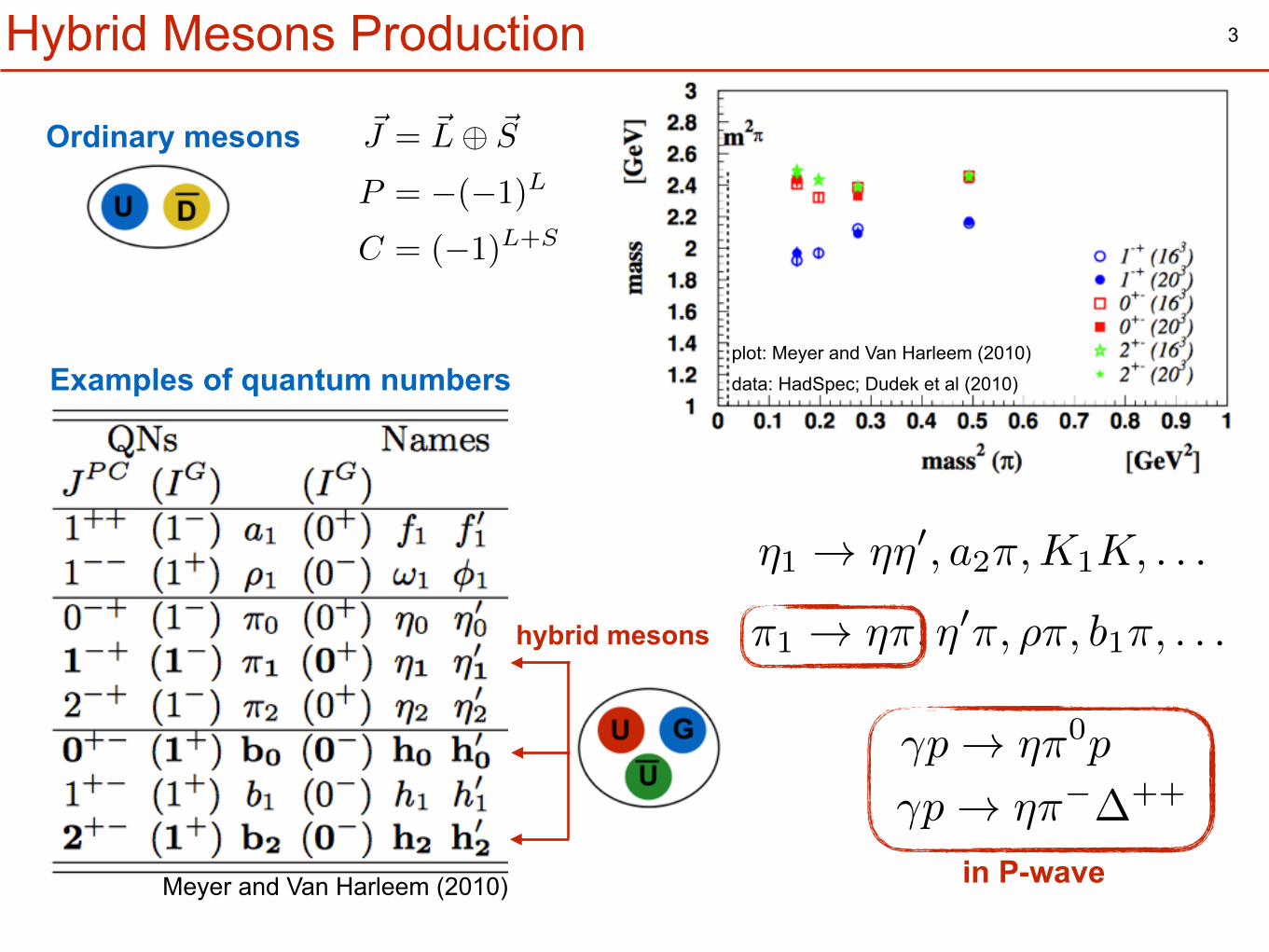
⇡1 ! ⌘⇡, ⌘0⇡, ⇢⇡, b1⇡, . . .

⌘1 ! ⌘⌘0, a2⇡,K1K, . . .

�p ! ⌘⇡��++

�p ! ⌘⇡0p

in P-wave

4

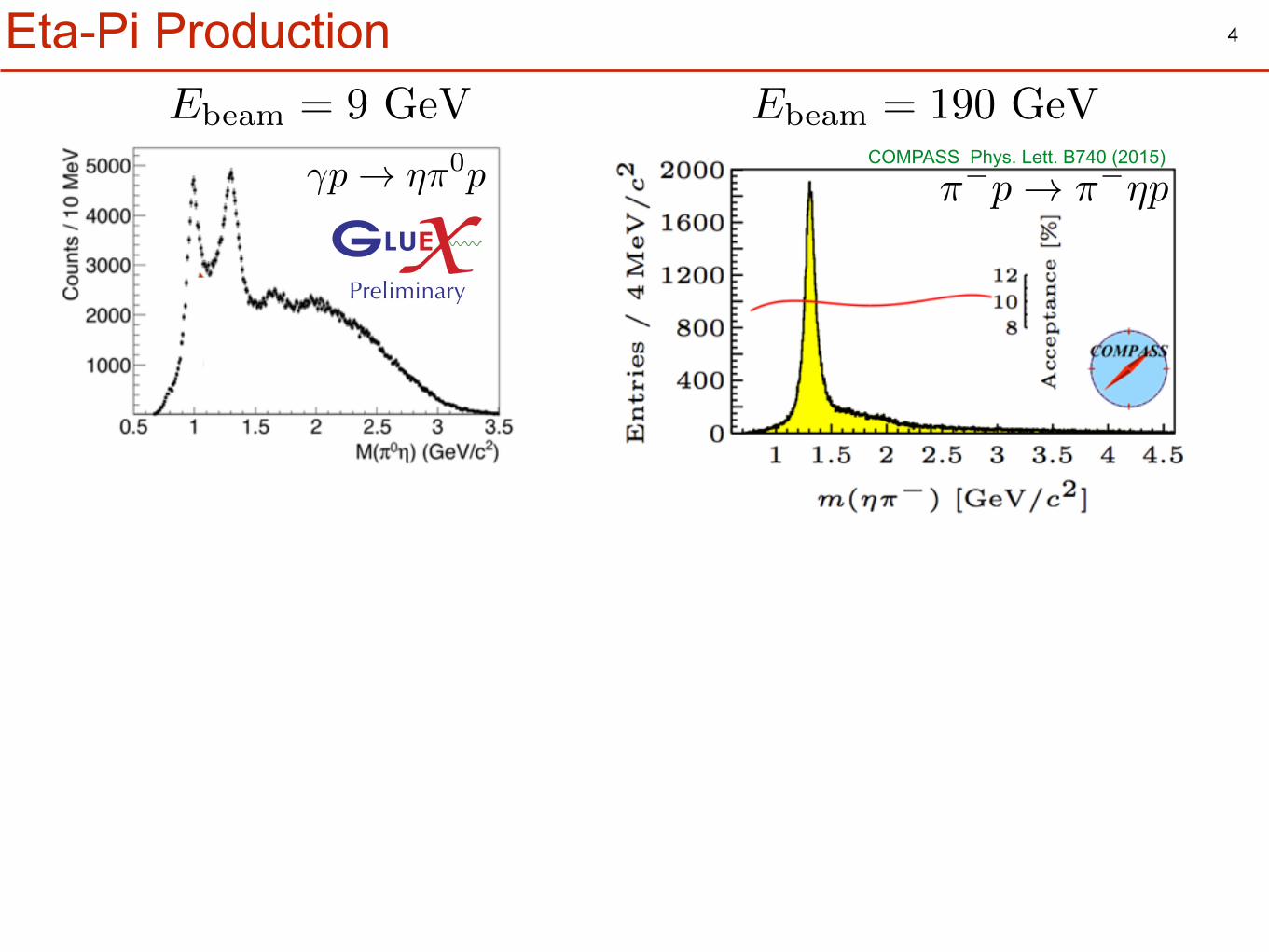
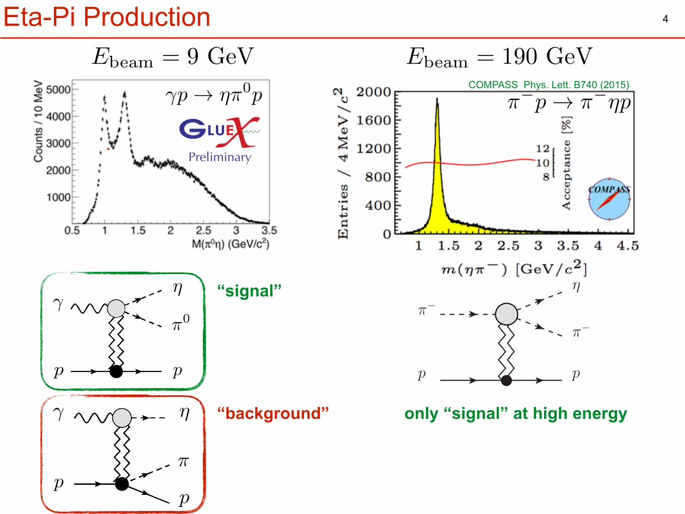
COMPASS Phys. Lett. B740 (2015)

Ebeam = 190 GeVEbeam = 9 GeV

Eta-Pi Production

�p ! ⌘⇡0p ⇡�p ! ⇡�⌘p

π−

p

η, η′

π−

Pp

⌘

p

�

p

⇡0

�

p⇡

⌘

p

“signal”

“background” only “signal” at high energy

4


Ebeam = 190 GeVEbeam = 9 GeV

Eta-Pi Production

�p ! ⌘⇡0p ⇡�p ! ⇡�⌘p

5

�

p⇡

⌘

p

⇡

⌘

p

�

p

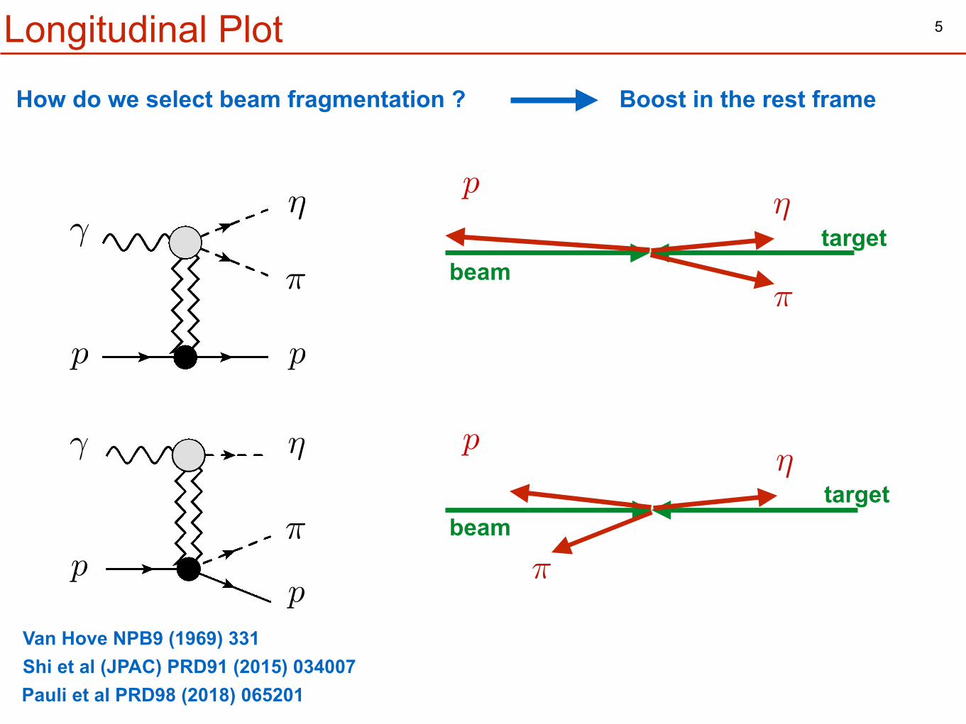
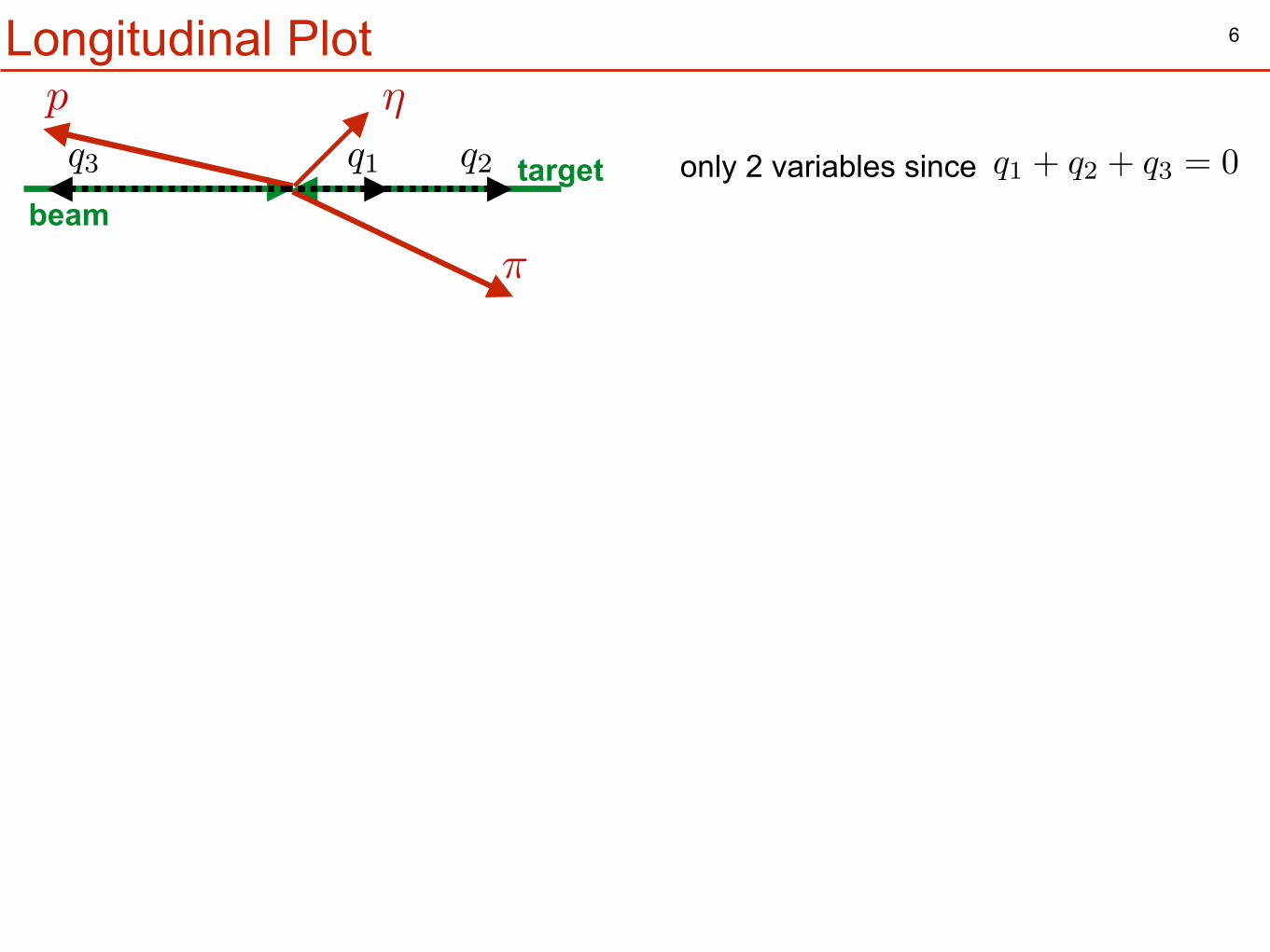
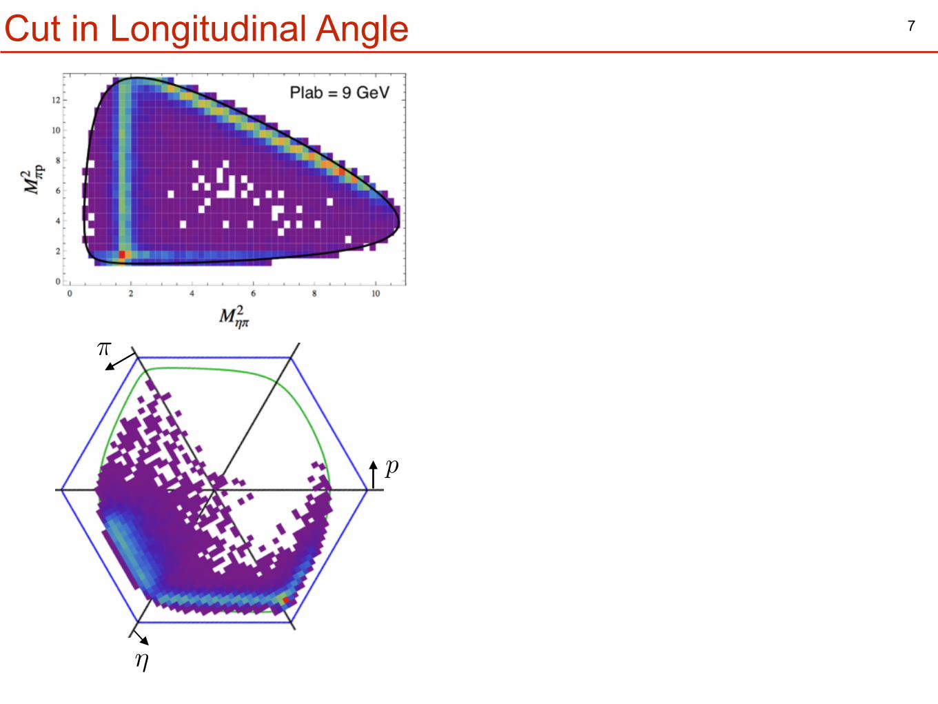
Longitudinal Plot

How do we select beam fragmentation ? Boost in the rest frame

p

beamtarget

⌘

⇡

p

beamtarget

⌘

⇡

Pauli et al PRD98 (2018) 065201Shi et al (JPAC) PRD91 (2015) 034007Van Hove NPB9 (1969) 331

6Longitudinal Plotp

beamtarget

⌘

⇡

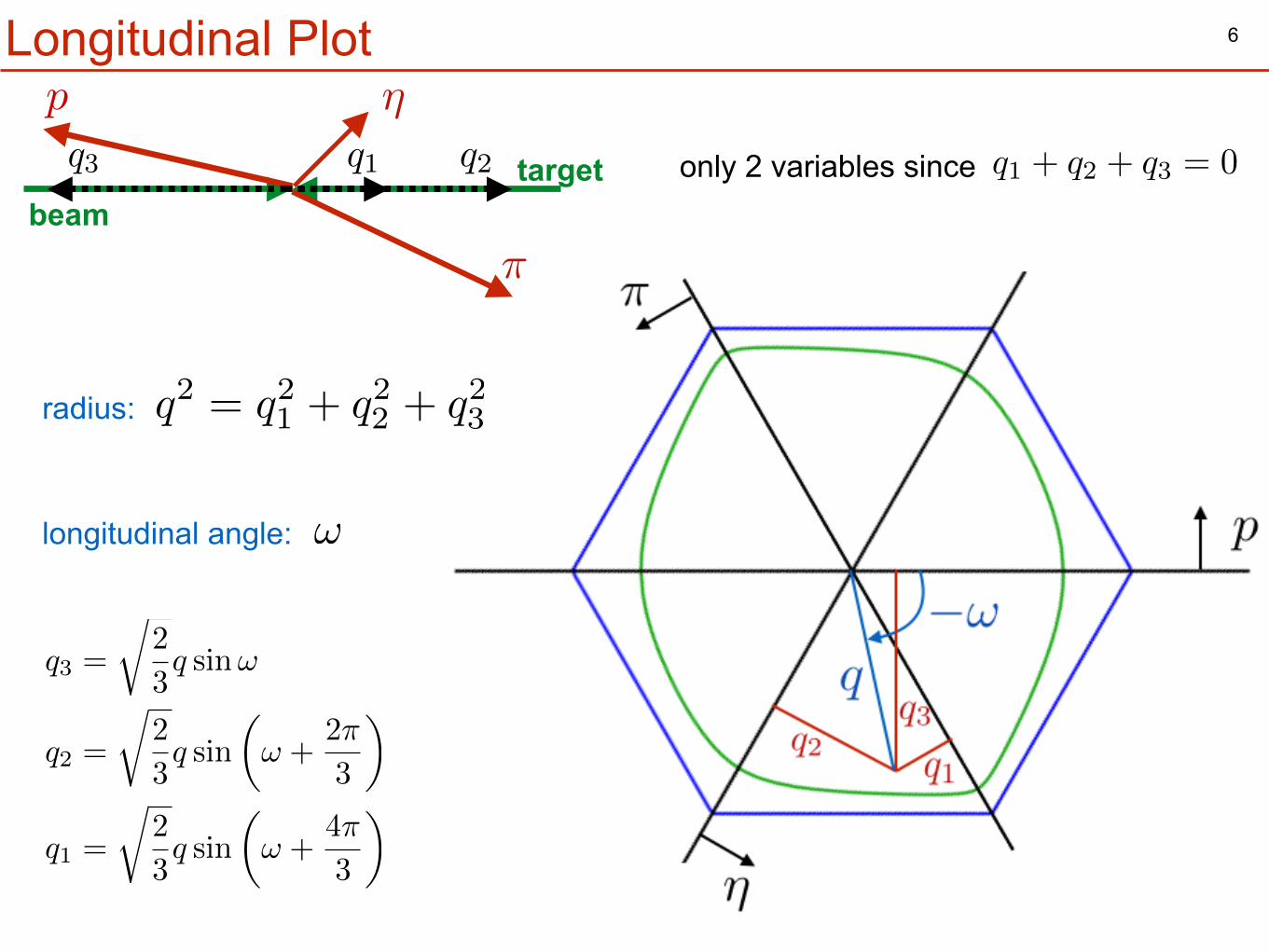
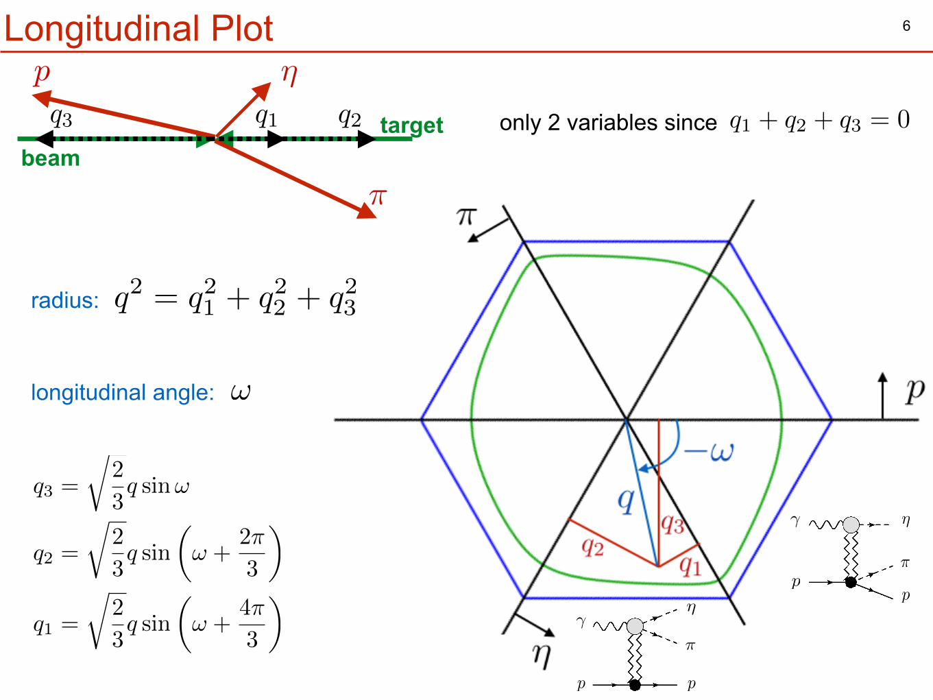
q1 + q2 + q3 = 0only 2 variables sinceq1 q2q3

6Longitudinal Plotp

beamtarget

⌘

⇡


radius: q2 = q21 + q22 + q23

longitudinal angle: !

q3 =

r2

3q sin!

q2 =

r2

3q sin

✓! +

2⇡

3

◆

q1 =

r2

3q sin

✓! +

4⇡

3

◆

6Longitudinal Plotp

beamtarget

⌘

⇡


�

p⇡

⌘

p

⇡

⌘

p

�

p

radius: q2 = q21 + q22 + q23

longitudinal angle: !

q3 =

r2

3q sin!

q2 =

r2

3q sin

✓! +

2⇡

3

◆

q1 =

r2

3q sin

✓! +

4⇡

3

◆

7

⌘

⇡

p

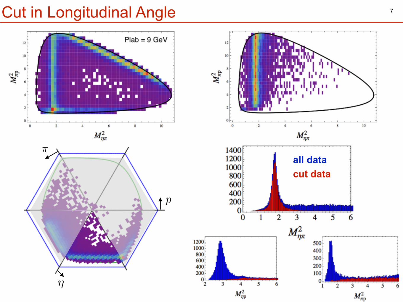
Cut in Longitudinal Angle

7

⌘

⇡

p

Cut in Longitudinal Angle

all datacut data

8

8

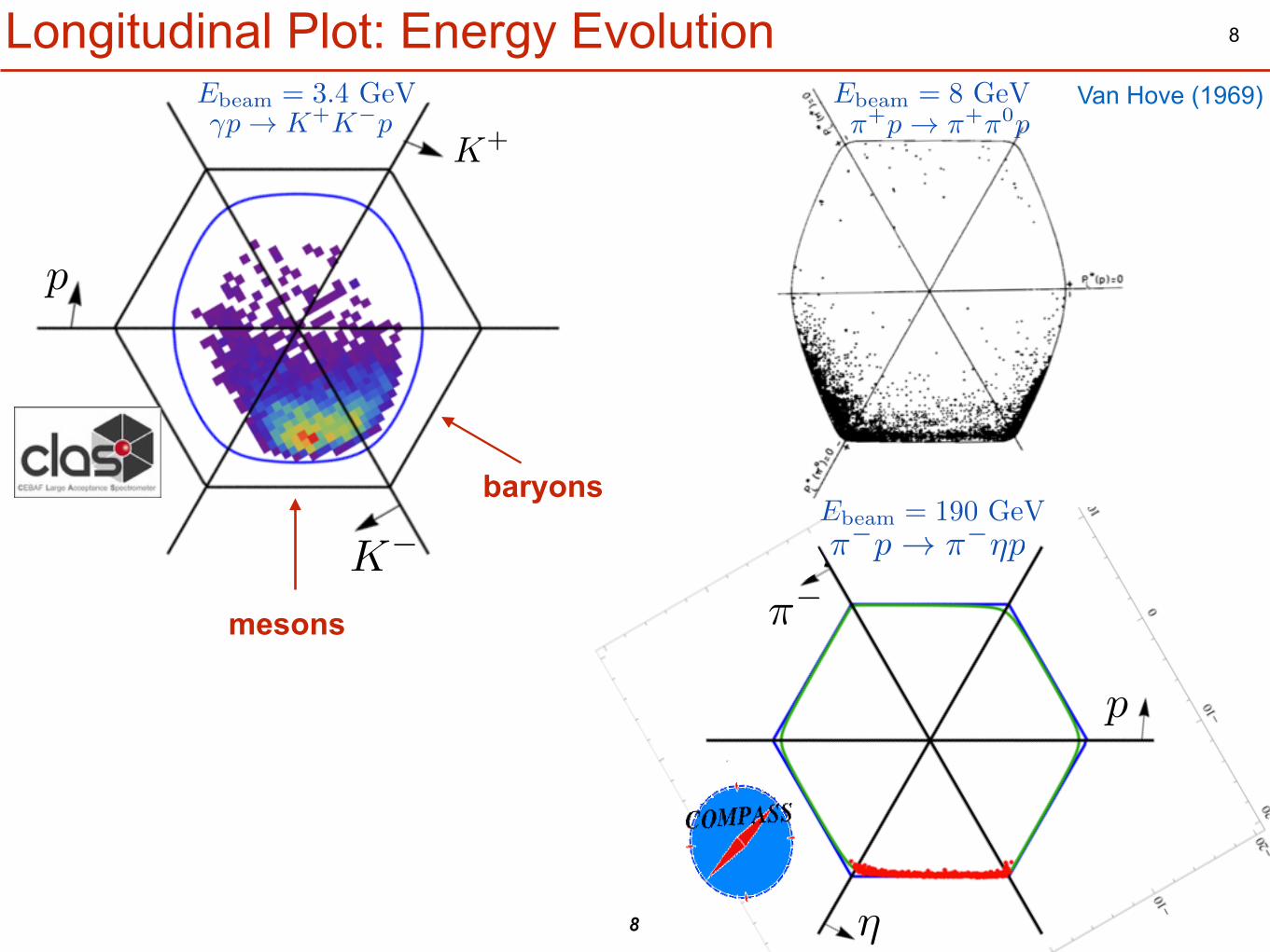
Longitudinal Plot: Energy EvolutionVan Hove (1969)

K+

K�

p

⌘

⇡�

p

mesons

baryons

⇡+p ! ⇡+⇡0p

⇡�p ! ⇡�⌘p

�p ! K+K�pEbeam = 3.4 GeV Ebeam = 8 GeV

Ebeam = 190 GeV

3− 2− 1− 0 1 2 33−

2−

1−

0

1

2

3

pq

ηq 0π

q

0πη

ηp0πp

GlueX Spring 2017 p0πη → p γ

preliminary

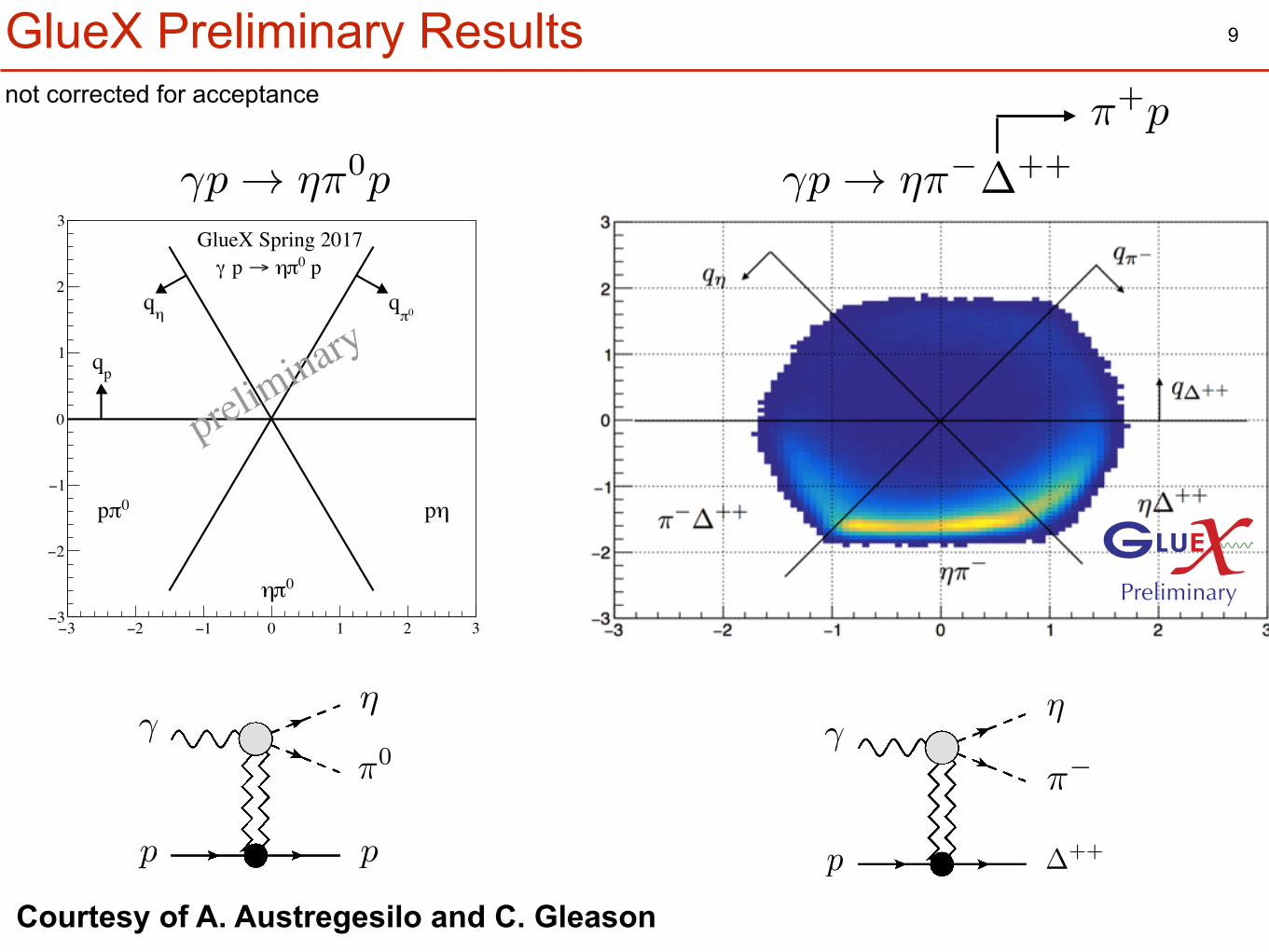
9GlueX Preliminary Results

�p ! ⌘⇡0p �p ! ⌘⇡��++

⇡+p

Courtesy of A. Austregesilo and C. Gleason

⌘

p

�

p

⇡0

⌘�

p

⇡�

�++

not corrected for acceptance

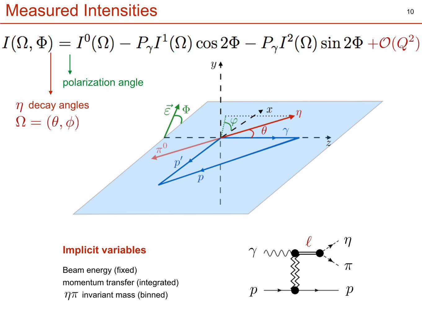
10Measured Intensities

Implicit variables

Beam energy (fixed)momentum transfer (integrated)

invariant mass (binned)⌘⇡

⇡

⌘�

p p

`

polarization angle

decay angles

⌦ = (✓,�)⌘

+O(Q2)

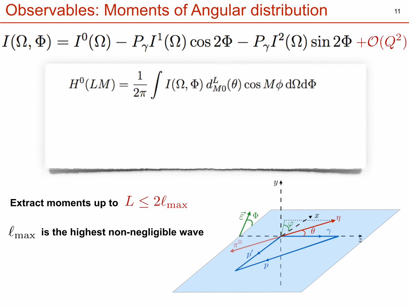
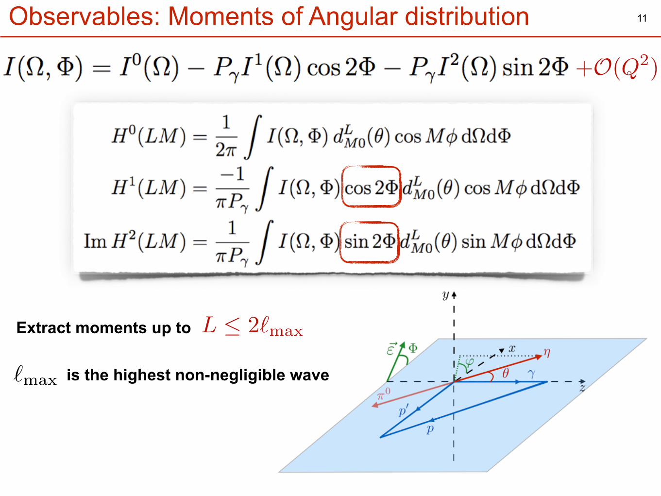
11Observables: Moments of Angular distribution

L 2`max

`max

is the highest non-negligible wave

Extract moments up to

+O(Q2)

11Observables: Moments of Angular distribution

L 2`max

`max

is the highest non-negligible wave

Extract moments up to

+O(Q2)

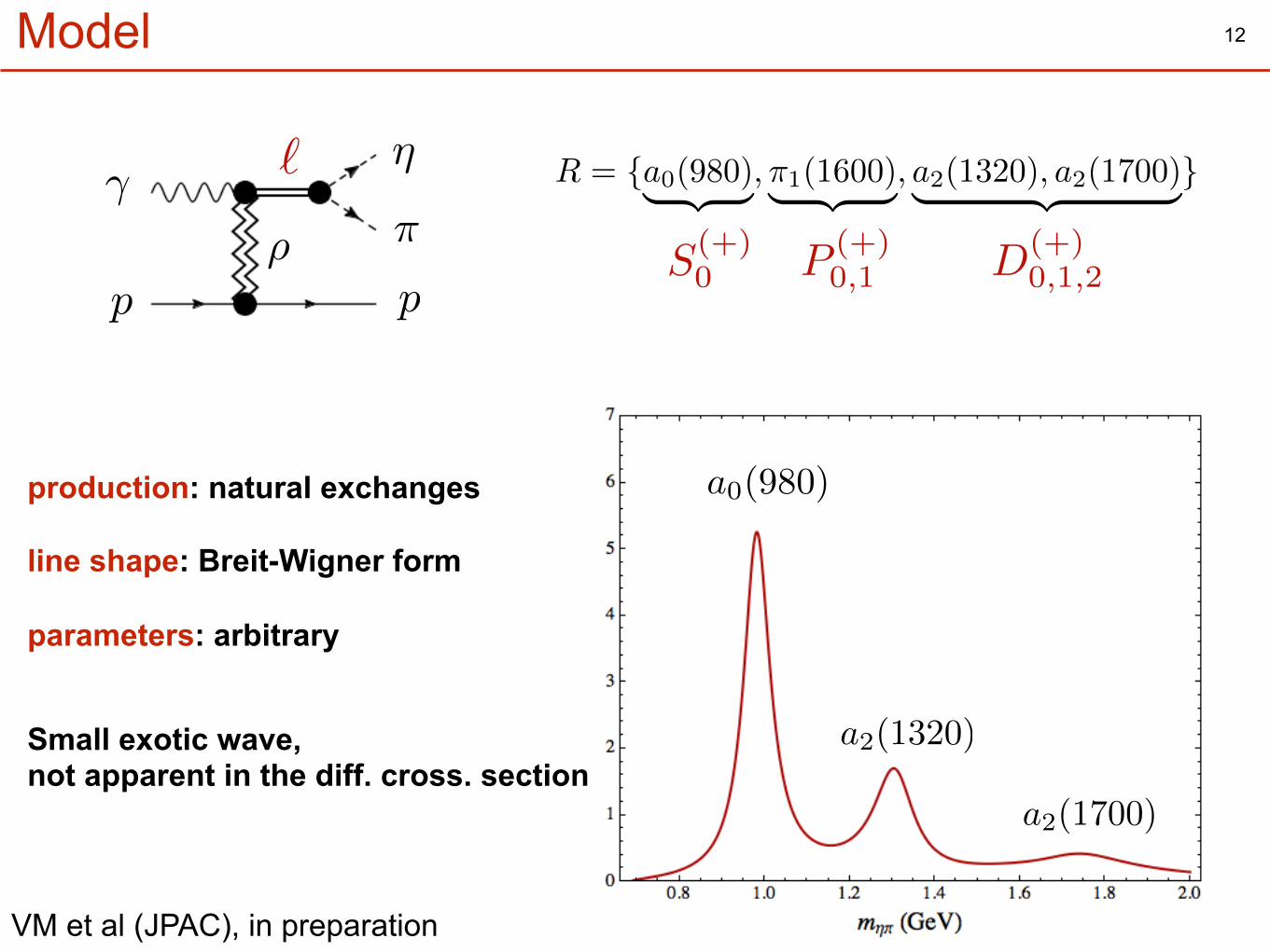
12Model

VM et al (JPAC), in preparation

R = {a0(980)| {z },⇡1(1600)| {z }, a2(1320), a2(1700)| {z }}

production: natural exchanges a0(980)

a2(1320)

a2(1700)

line shape: Breit-Wigner form

parameters: arbitrary

Small exotic wave, not apparent in the diff. cross. section

⇢ ⇡

⌘�

p p

`

S(+)0 P (+)

0,1 D(+)0,1,2

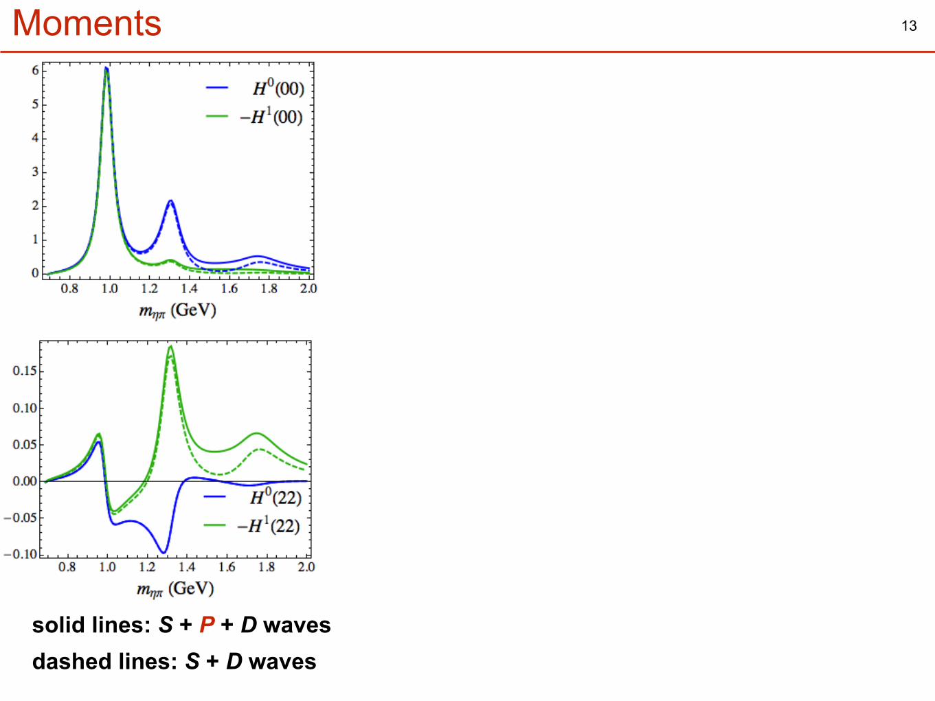
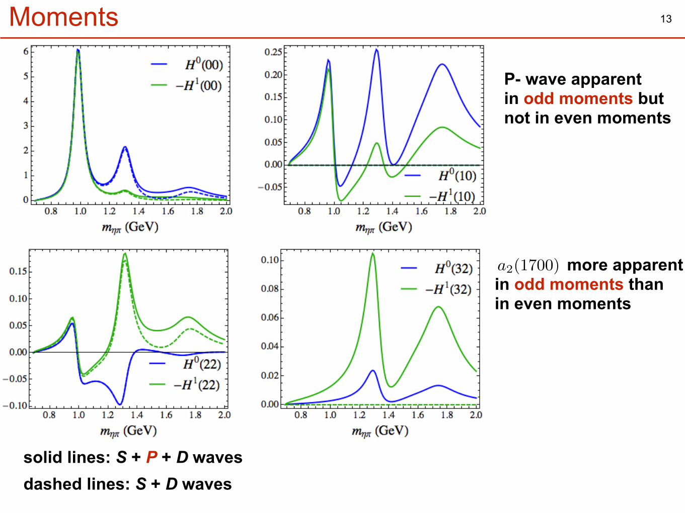
13Moments

solid lines: S + P + D wavesdashed lines: S + D waves

P- wave apparent in odd moments but not in even moments

more apparent in odd moments than in even moments

a2(1700)

13Moments

solid lines: S + P + D wavesdashed lines: S + D waves

P- wave apparent in odd moments but not in even moments

more apparent in odd moments than in even moments

a2(1700)

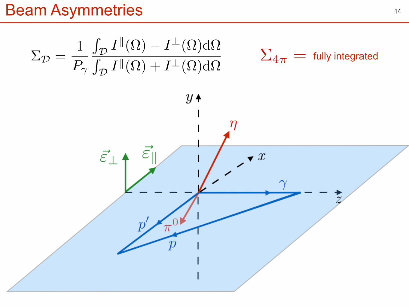
14Beam Asymmetries

⌃D =1

P�

RD Ik(⌦)� I?(⌦)d⌦RD Ik(⌦) + I?(⌦)d⌦

⌃4⇡ = fully integrated

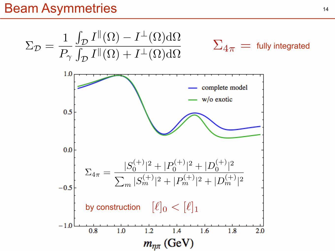
14Beam Asymmetries

⌃D =1

P�

RD Ik(⌦)� I?(⌦)d⌦RD Ik(⌦) + I?(⌦)d⌦

⌃4⇡ = fully integrated

⌃4⇡ =|S(+)

0 |2 + |P (+)0 |2 + |D(+)

0 |2P

m |S(+)m |2 + |P (+)

m |2 + |D(+)m |2

by construction [`]0 < [`]1

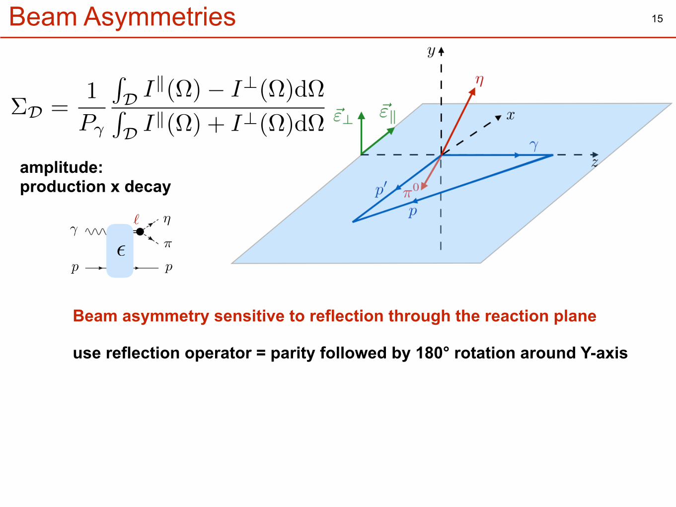
15Beam Asymmetries

amplitude: production x decay

Beam asymmetry sensitive to reflection through the reaction plane

⌃D =1

P�

RD Ik(⌦)� I?(⌦)d⌦RD Ik(⌦) + I?(⌦)d⌦

use reflection operator = parity followed by 180° rotation around Y-axis

⇡

⌘�

p p

`

✏

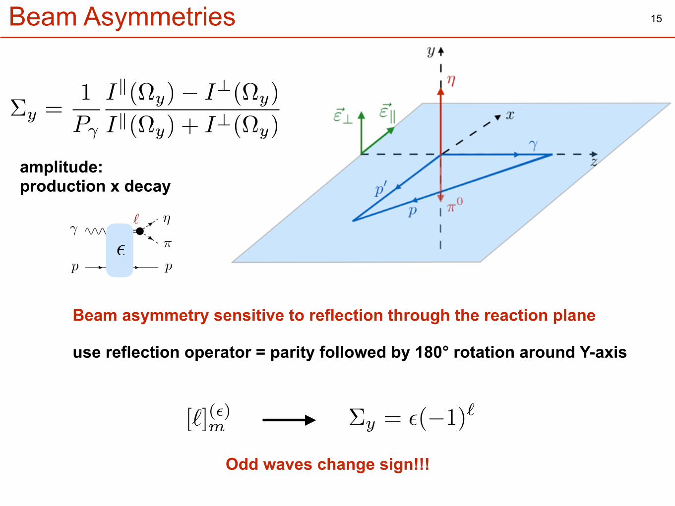
15Beam Asymmetries

amplitude: production x decay

Beam asymmetry sensitive to reflection through the reaction plane

⌃y =1

P�

Ik(⌦y)� I?(⌦y)

Ik(⌦y) + I?(⌦y)

use reflection operator = parity followed by 180° rotation around Y-axis

⌃y = ✏(�1)`[`](✏)m

Odd waves change sign!!!

⇡

⌘�

p p

`

✏

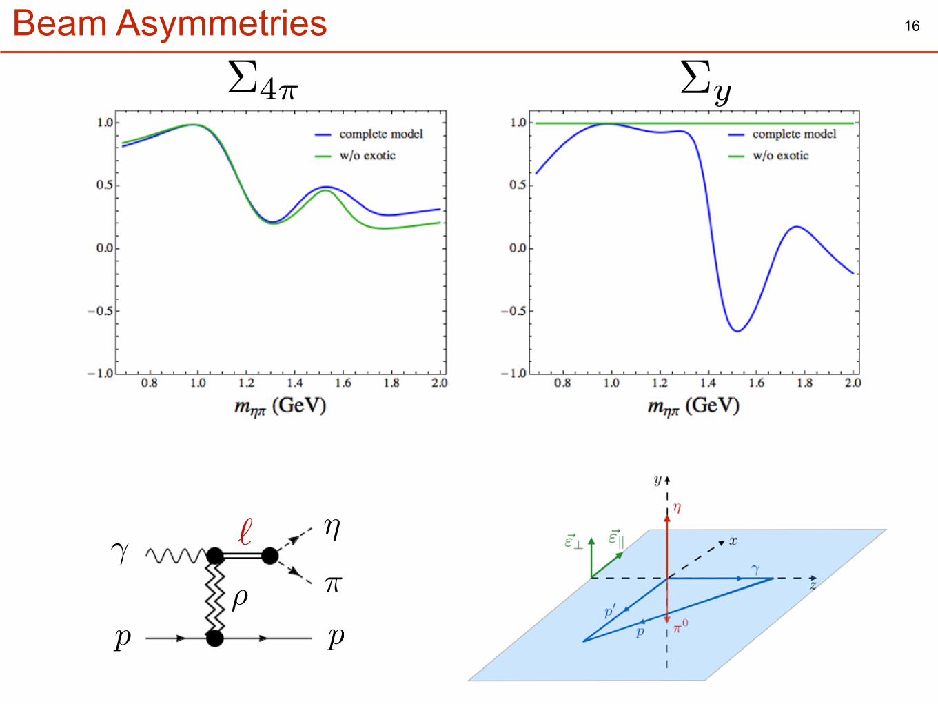
16

⌃4⇡ ⌃y

Beam Asymmetries

⇢ ⇡

⌘�

p p

`

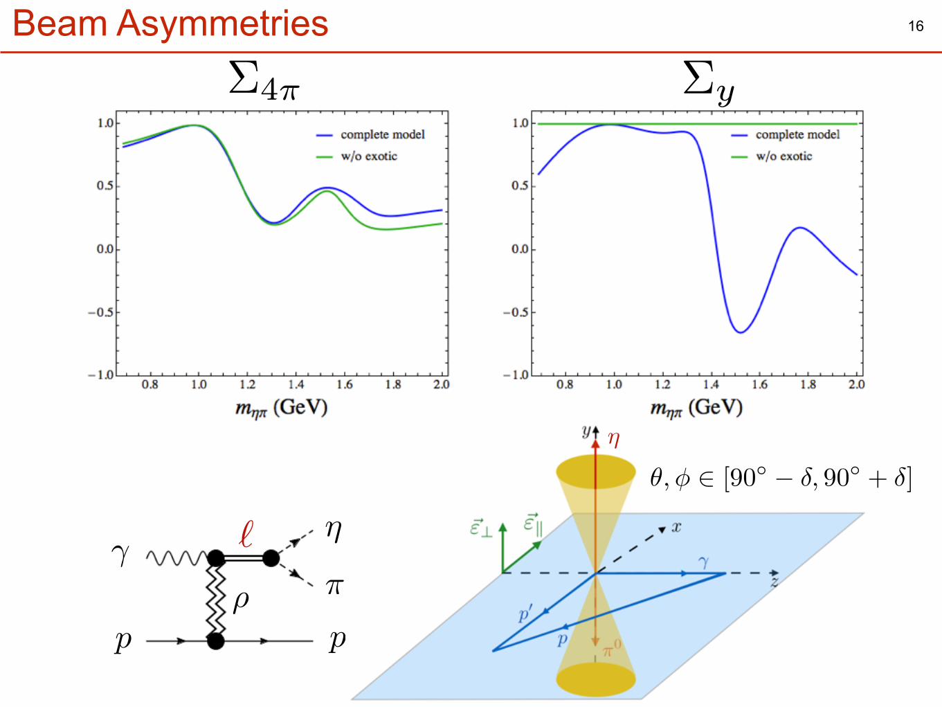
16

⌃4⇡ ⌃y

Beam Asymmetries

⇢ ⇡

⌘�

p p

`

⌘

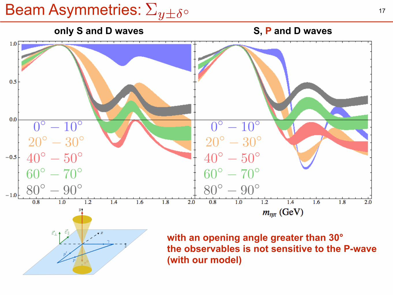
✓,� 2 [90� � �, 90� + �]

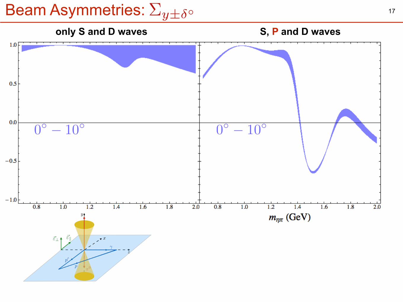
17

0� � 10� 0� � 10�

only S and D waves S, P and D waves

Beam Asymmetries: ⌃y±��

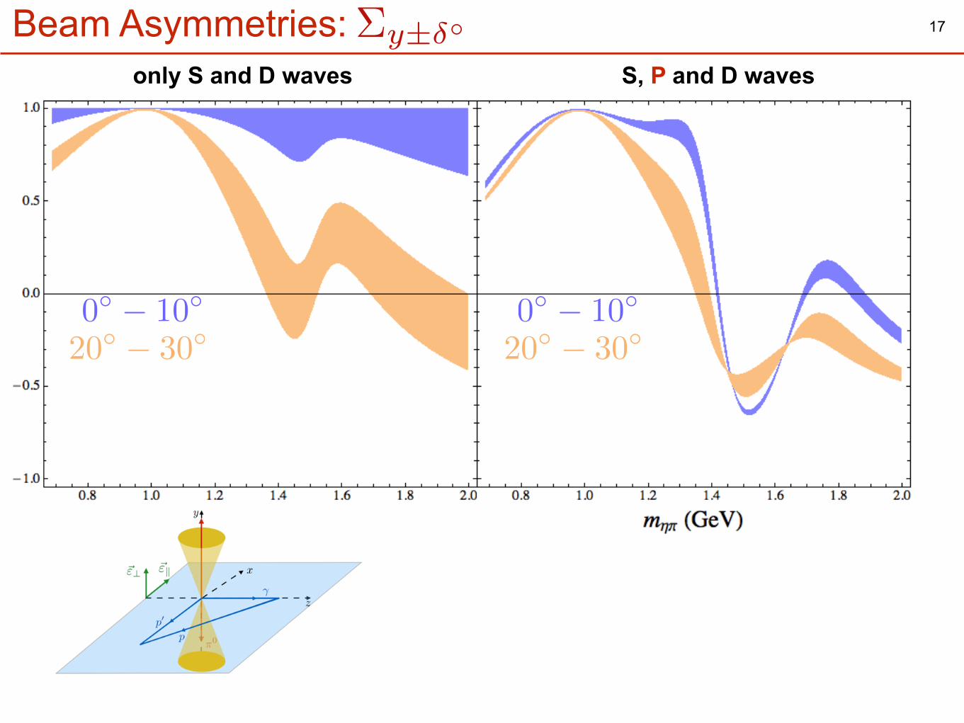
20� � 30� 20� � 30�

17

0� � 10� 0� � 10�


Beam Asymmetries: ⌃y±��

20� � 30� 20� � 30�

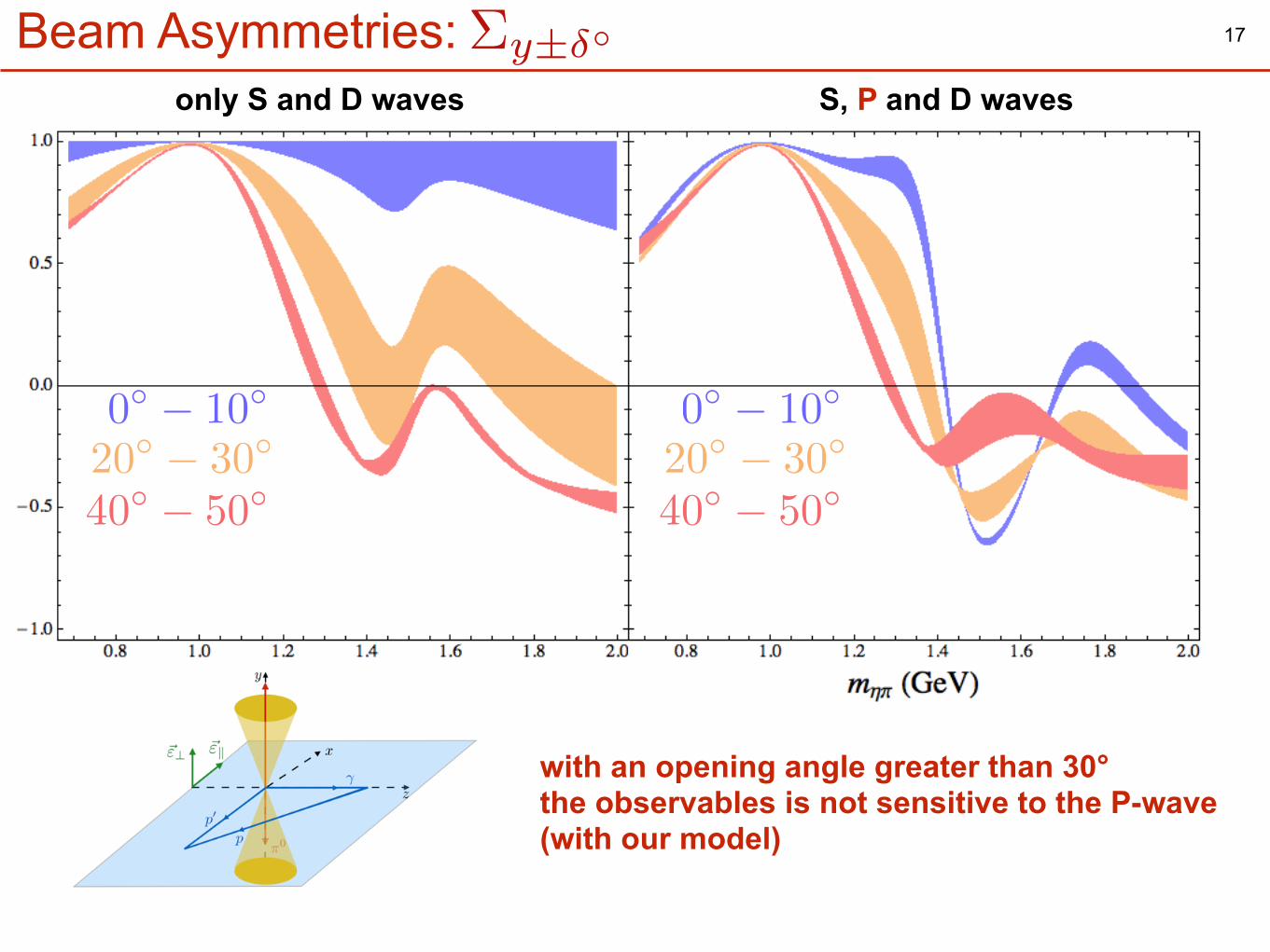
17

0� � 10� 0� � 10�

40� � 50� 40� � 50�


Beam Asymmetries:

with an opening angle greater than 30° the observables is not sensitive to the P-wave (with our model)

⌃y±��

20� � 30� 20� � 30�

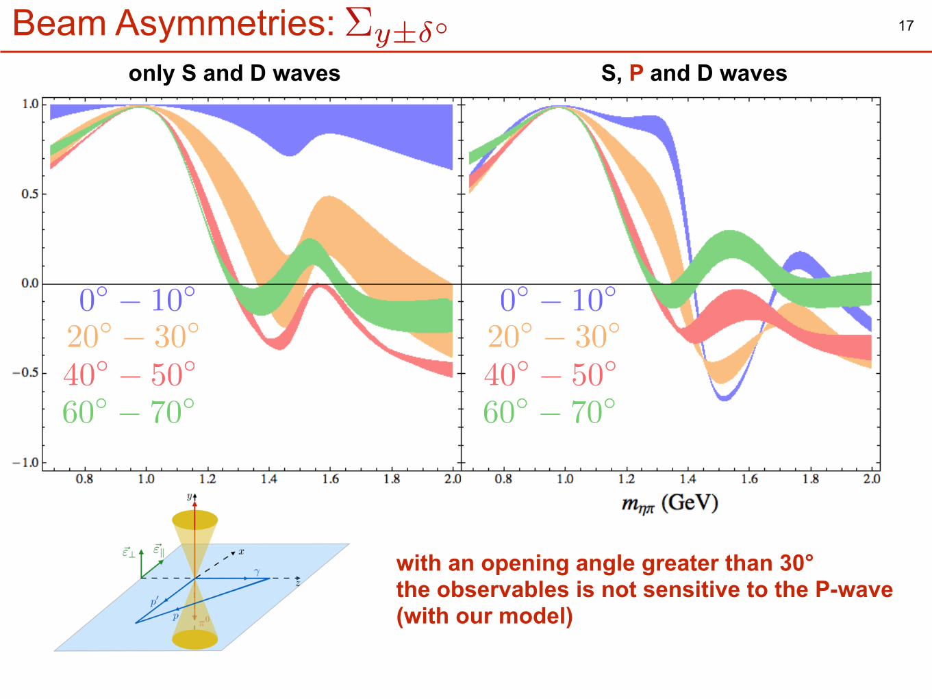
17

0� � 10� 0� � 10�

40� � 50� 40� � 50�

60� � 70� 60� � 70�


Beam Asymmetries:


⌃y±��

20� � 30� 20� � 30�

17

0� � 10� 0� � 10�

40� � 50� 40� � 50�

60� � 70� 60� � 70�

80� � 90� 80� � 90�


Beam Asymmetries:


⌃y±��

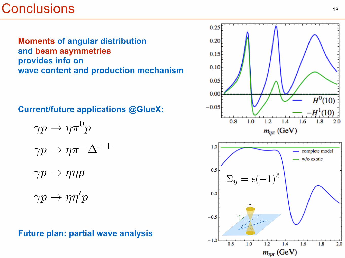
18Conclusions

⌘

⌃y = ✏(�1)`

Moments of angular distribution and beam asymmetries provides info on wave content and production mechanism

�p ! ⌘⇡��++

�p ! ⌘⇡0p

�p ! ⌘⌘p

�p ! ⌘⌘0p

Current/future applications @GlueX:

Future plan: partial wave analysis

19

Backup Slides

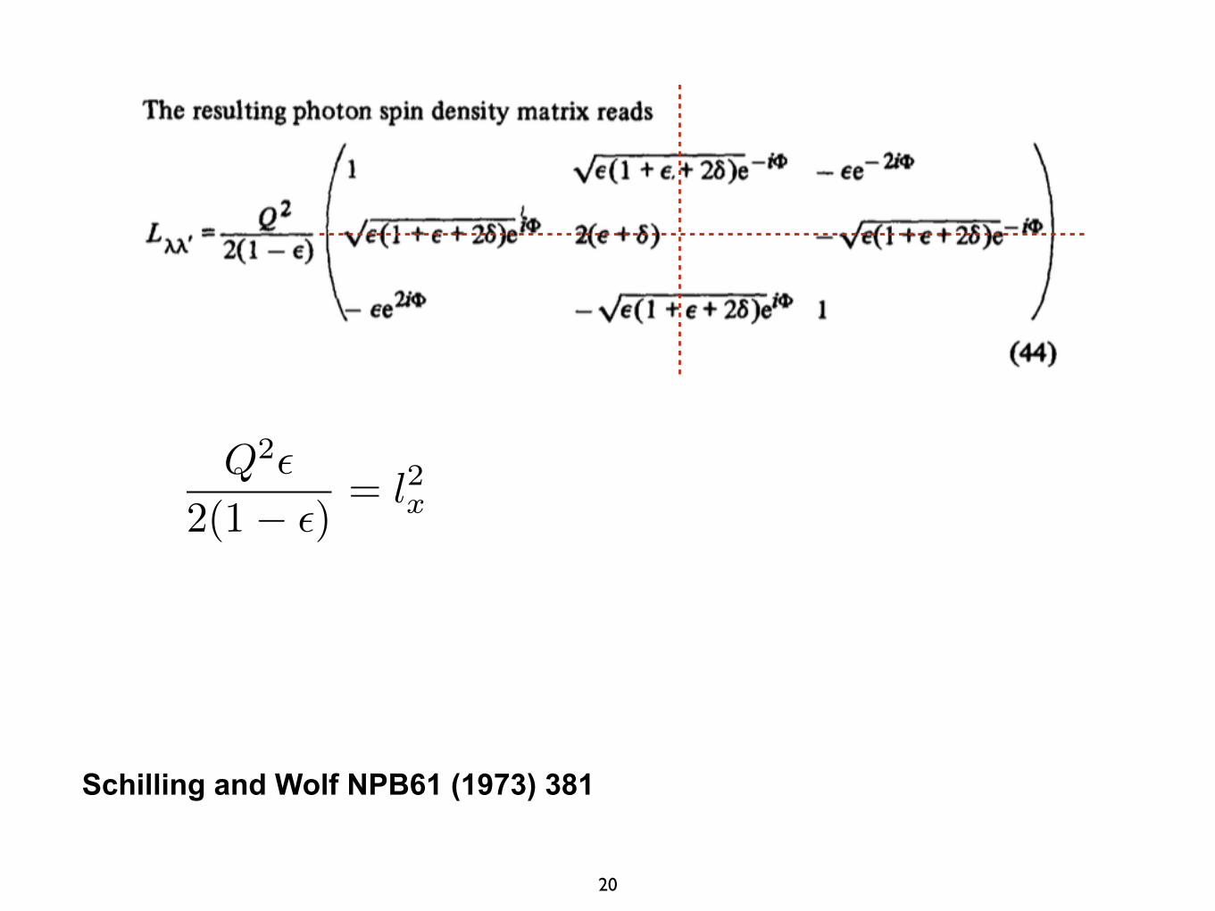
20

Q2✏

2(1� ✏)= l2

x

Schilling and Wolf NPB61 (1973) 381

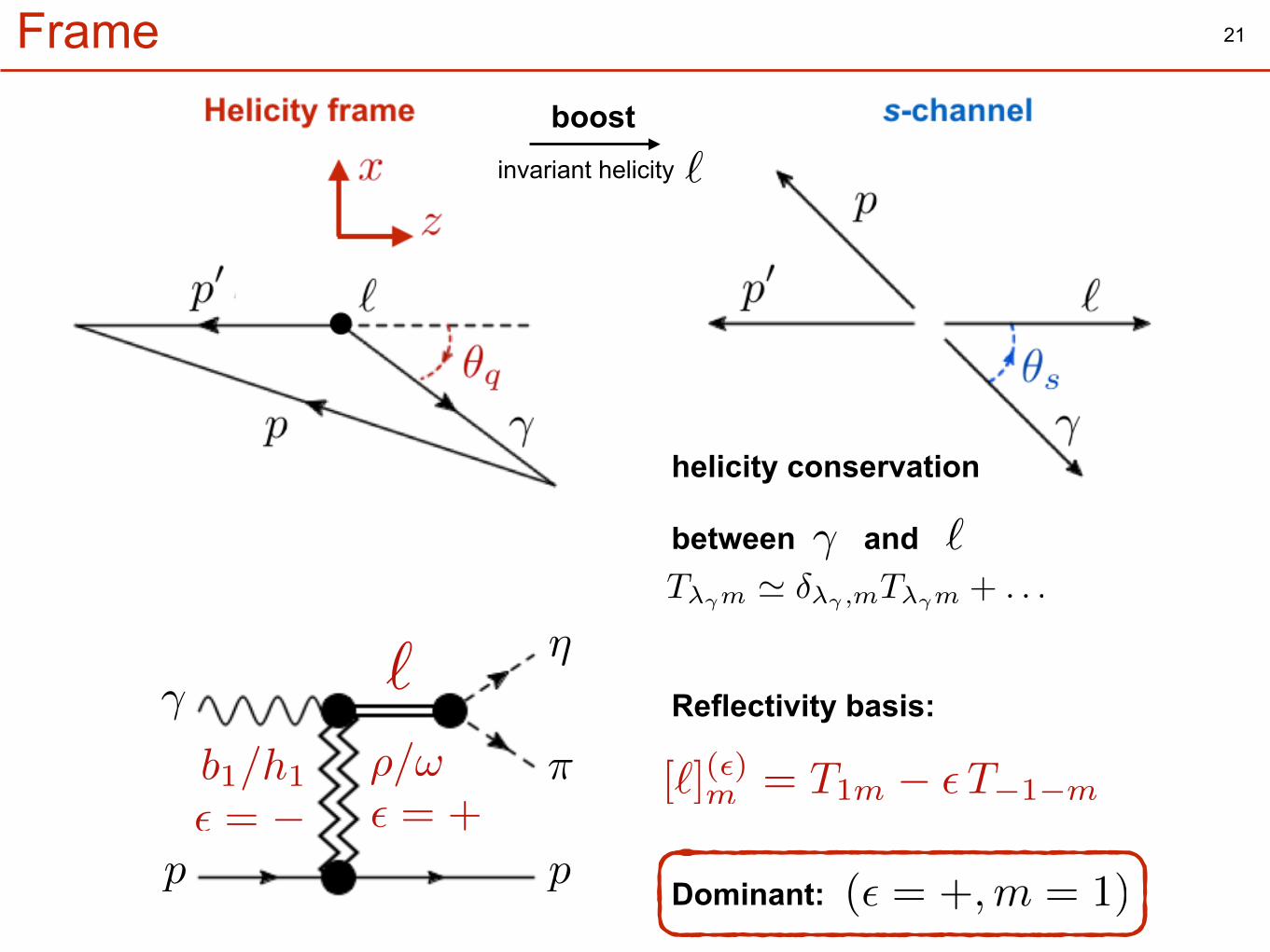
21Frame

`

⇡

⌘�

p p

boost

helicity conservation

between and� `

b1/h1

✏ = �⇢/!✏ = +

[`](✏)m = T1m � ✏T�1�m

Reflectivity basis:

invariant helicity `

Dominant: (✏ = +,m = 1)

T��m ' �� ,mT��m + . . .

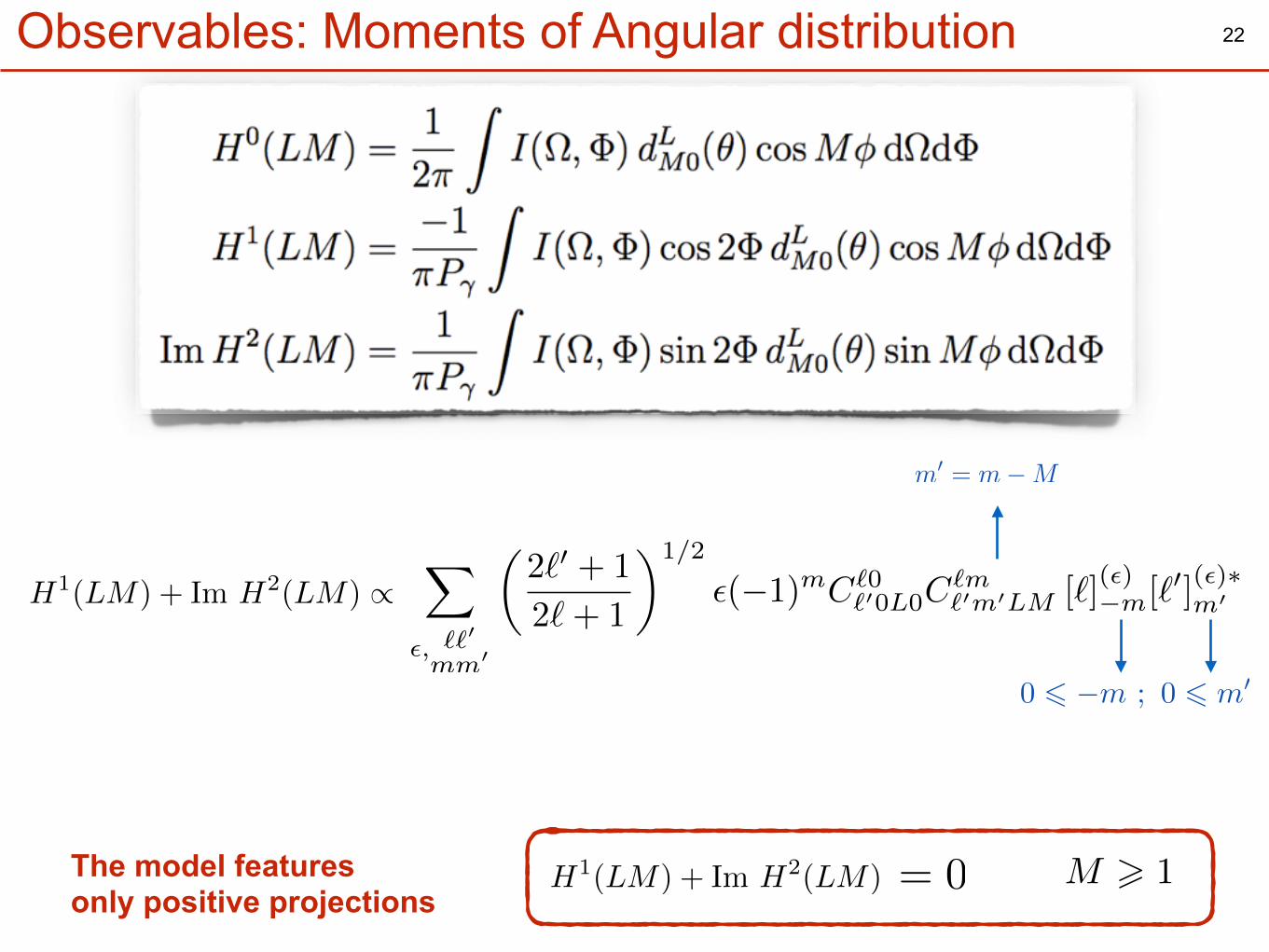
22

X

✏, ``0

mm0

✓2`0 + 1

2`+ 1

◆1/2

✏(�1)mC`0`00L0C

`m`0m0LM [`](✏)�m[`0](✏)⇤m0H1(LM) + Im H2(LM) /

H1(LM) + Im H2(LM) /= 0The model features only positive projections

m0 = m�M

0 6 �m ; 0 6 m0

M > 1

Observables: Moments of Angular distribution

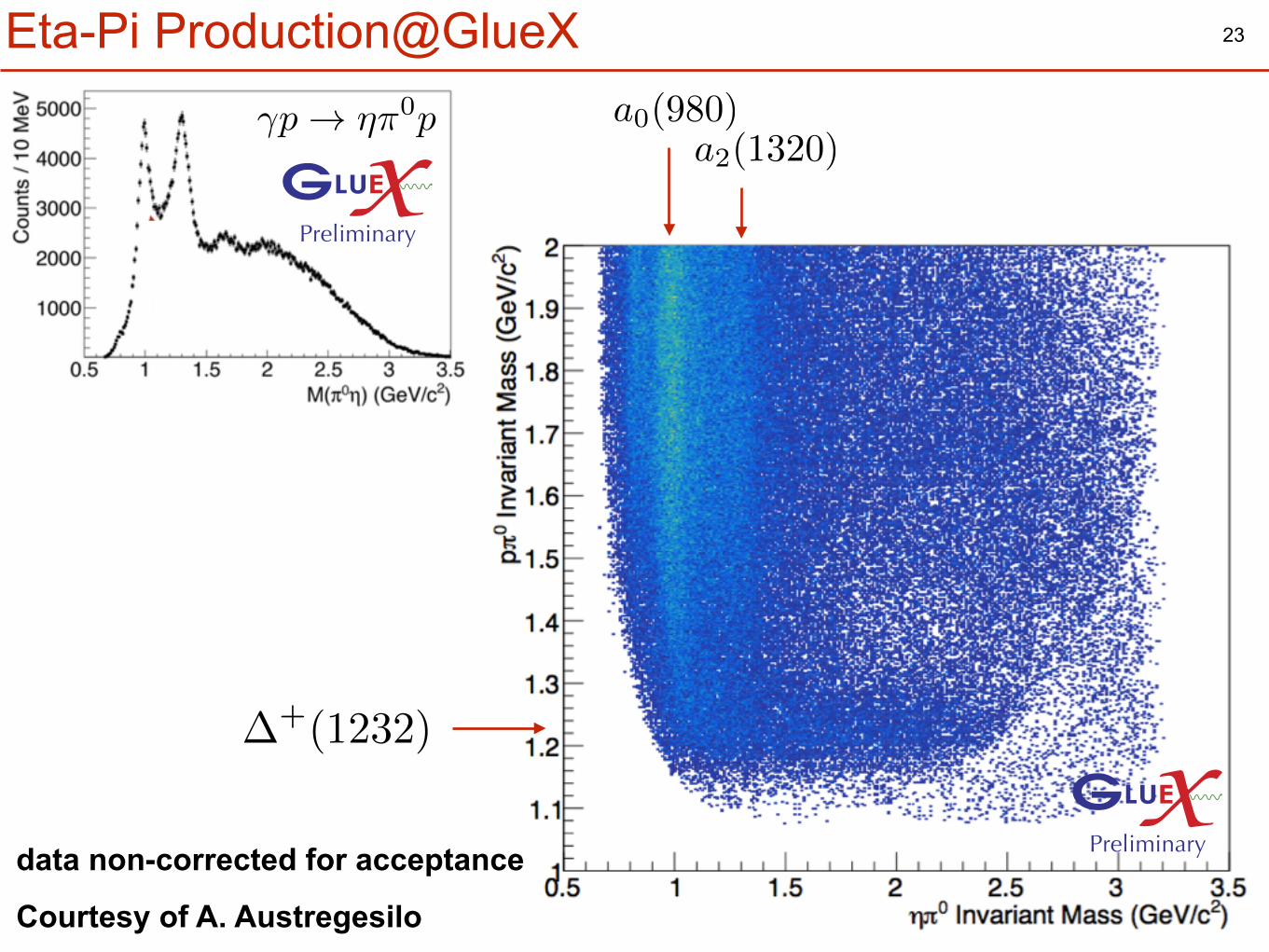
23

�p ! ⌘⇡0p

Courtesy of A. Austregesilo

a0(980)a2(1320)

�+(1232)

Eta-Pi Production@GlueX

data non-corrected for acceptance

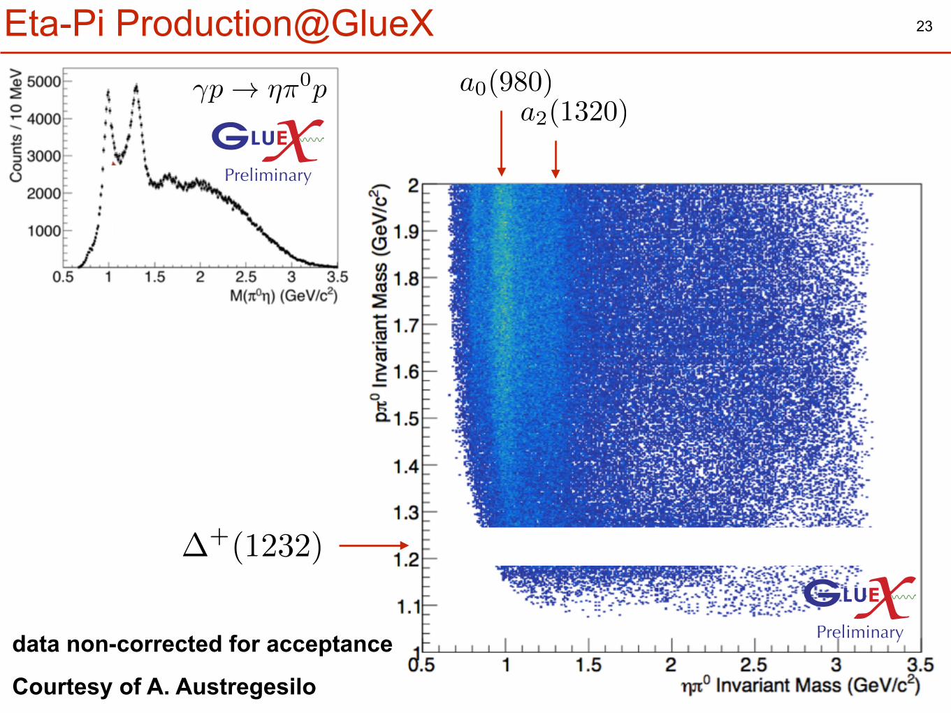
23

�p ! ⌘⇡0p

Courtesy of A. Austregesilo

a0(980)a2(1320)

�+(1232)

Eta-Pi Production@GlueX

data non-corrected for acceptance

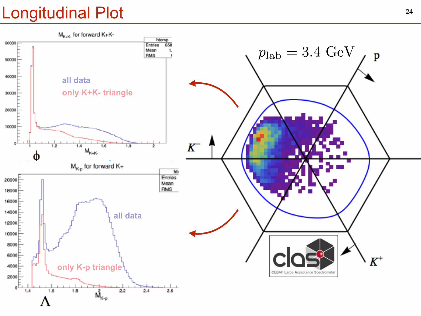
24Longitudinal Plot

only K+K- triangle

only K-p triangle

all data

all data

plab = 3.4 GeV

25

a

b

1

2

3

P

Y

⌘

⇡�⇡�

P + f

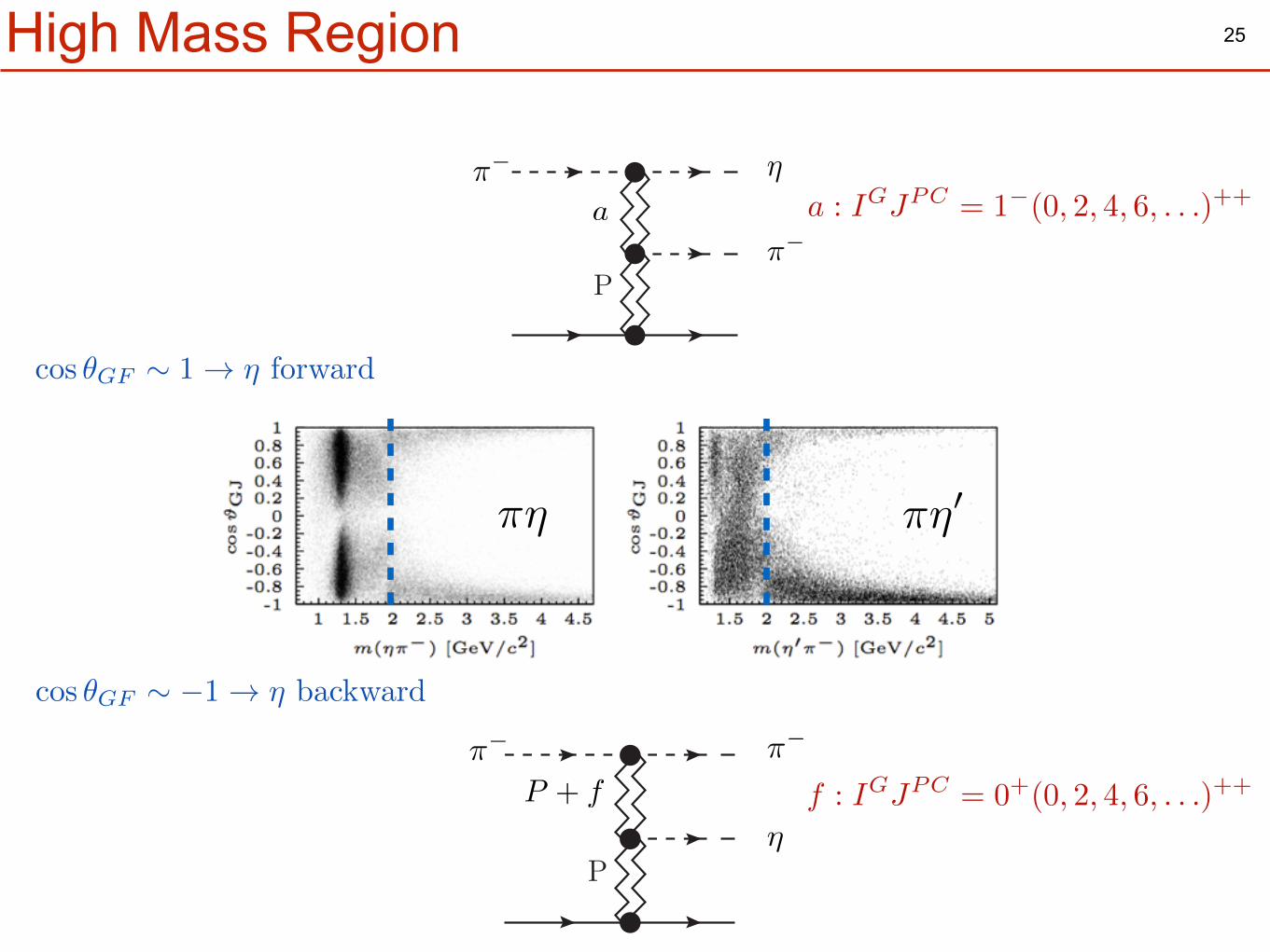
High Mass Region

⇡⌘ ⇡⌘0

a

b

1

2

3

P

Y⌘

⇡�a

⇡�

cos ✓GF ⇠ 1 ! ⌘ forward

cos ✓GF ⇠ �1 ! ⌘ backward

a : IGJPC = 1�(0, 2, 4, 6, . . .)++

f : IGJPC = 0+(0, 2, 4, 6, . . .)++

26

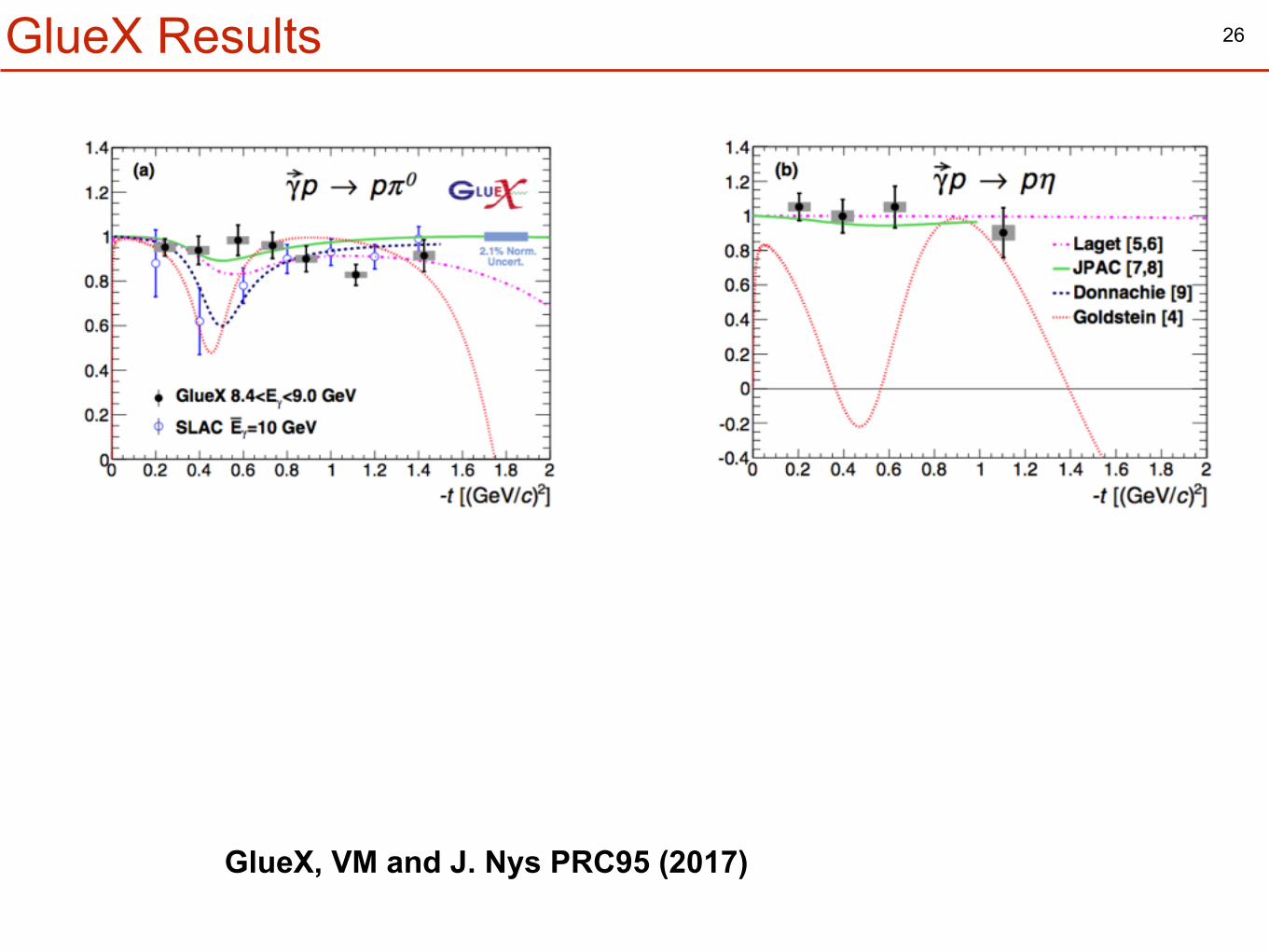
GlueX, VM and J. Nys PRC95 (2017)

GlueX Results

π−

p

η, η′

π−

Pp

⇡⌘ ⇡⌘0

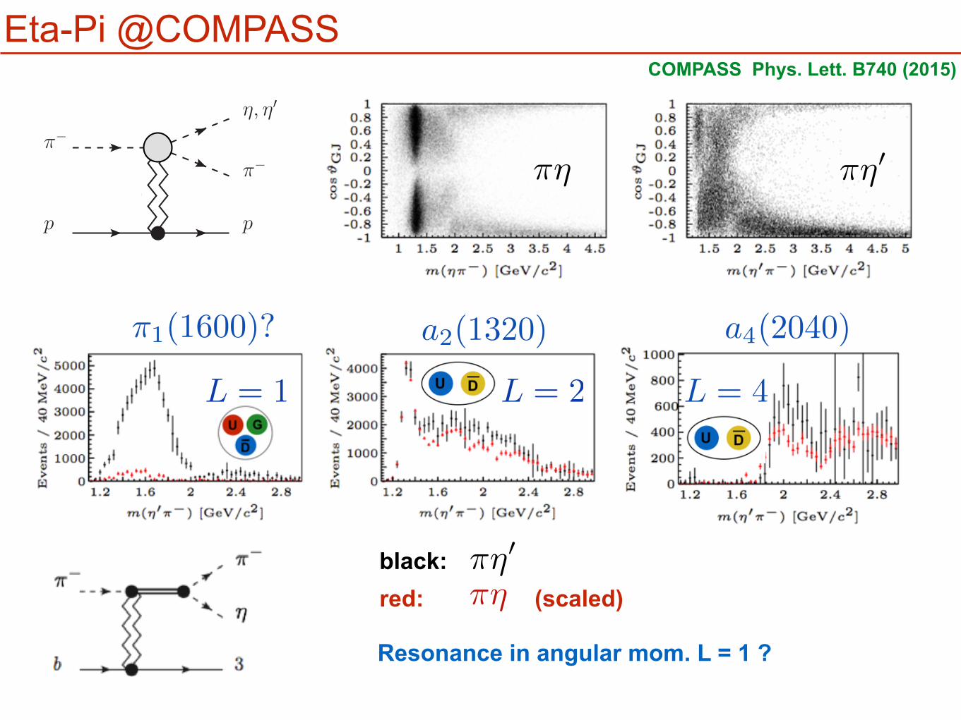
Eta-Pi @COMPASS

L = 1 L = 2

⇡1(1600)? a2(1320)

black: red: (scaled)

⇡⌘0

⇡⌘

Resonance in angular mom. L = 1 ?

L = 4

a4(2040)


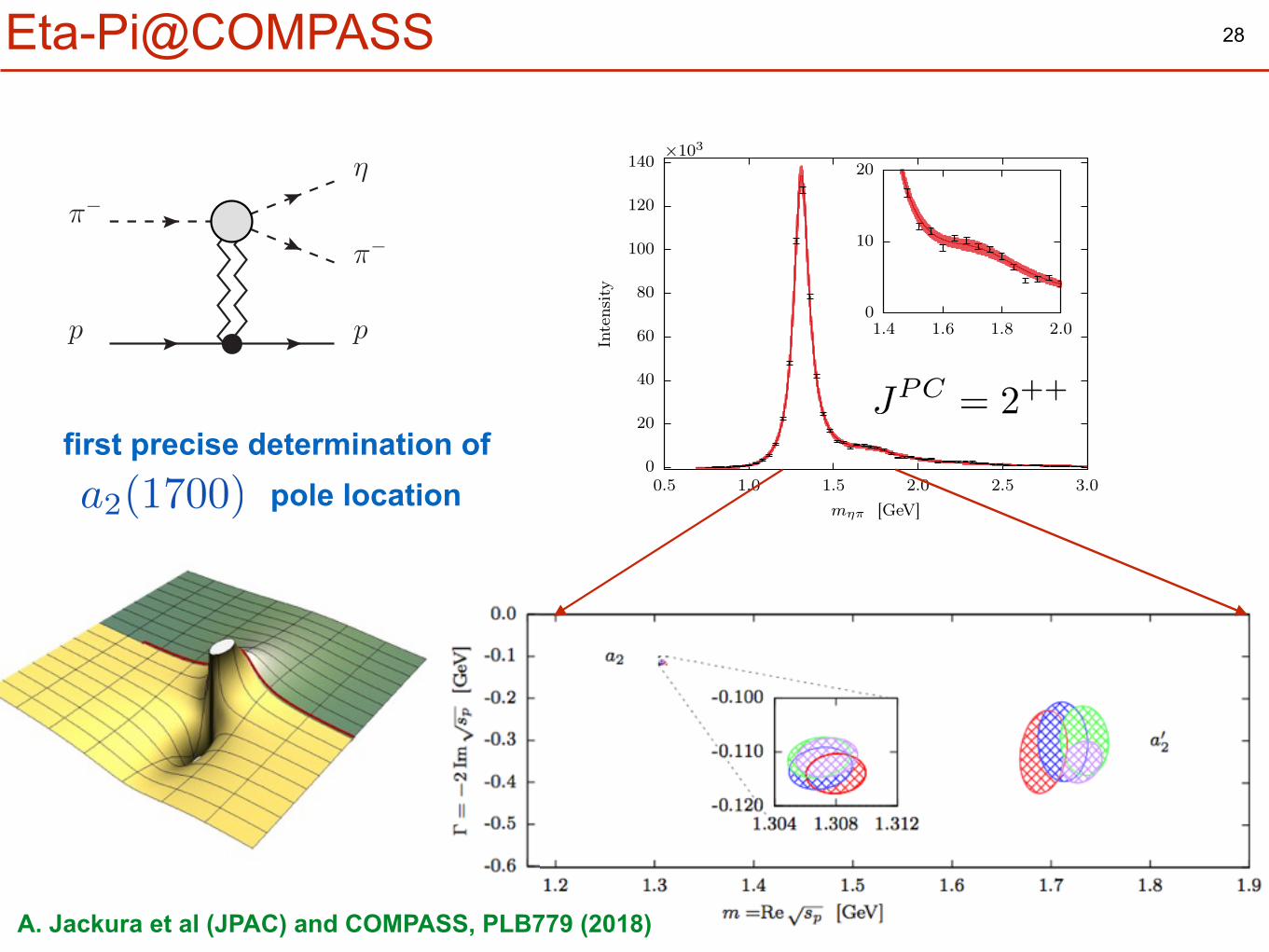
28Eta-Pi@COMPASS

0

20

40

60

80

100

120

140

0.5 1.0 1.5 2.0 2.5 3.0

Inte

nsity

mηπ [GeV]

×103

0

10

20

1.4 1.6 1.8 2.0

JPC = 2++

π−

p

η, η′

π−

Pp

A. Jackura et al (JPAC) and COMPASS, PLB779 (2018)

first precise determination ofpole locationa2(1700)

Ê Ê Ê

Ê

Ê

Ê Ê

Ê

Ê ÊÊ Ê

Ê

Ê

Ê

Ê Ê

Ê Ê ÊÊ Ê

Ê

Ê

Ê Ê Ê Ê Ê Ê

Ê

0.8 1.0 1.2 1.4 1.6 1.8 2.00

1000

2000

3000

4000

mhp HGeVL

Ê Ê Ê Ê Ê Ê Ê ÊÊ Ê

Ê

Ê

Ê

Ê

Ê

Ê

Ê

Ê

ÊÊ Ê Ê Ê Ê Ê Ê Ê Ê Ê Ê Ê Ê Ê Ê Ê Ê Ê Ê Ê Ê

0.8 1.0 1.2 1.4 1.6 1.8 2.00

20000

40000

60000

80000

100000

120000

mhp HGeVLÊ Ê

Ê ÊÊ Ê

ÊÊ Ê

ÊÊ Ê

Ê

ÊÊÊ Ê Ê

Ê Ê ÊÊÊ

Ê

Ê Ê

ÊÊÊÊ

Ê

Ê

ÊÊ

Ê

ÊÊ Ê

Ê

Ê

Ê Ê Ê ÊÊ Ê Ê

Ê Ê Ê Ê ÊÊ Ê Ê Ê Ê

Ê Ê ÊÊ Ê Ê Ê

Ê

0.8 1.0 1.2 1.4 1.6 1.8 2.0-200

-100

0

100

200

mhp HGeVL

Ê ÊÊÊÊ

Ê Ê Ê

Ê

Ê

ÊÊ Ê

Ê

Ê

Ê

Ê

Ê

Ê

ÊÊ Ê

Ê

Ê

ÊÊ

Ê Ê Ê Ê Ê Ê ÊÊ Ê Ê Ê Ê Ê ÊÊ Ê

Ê

ÊÊÊ

Ê

Ê

ÊÊ

ÊÊÊÊ Ê

Ê

Ê

Ê

Ê

Ê

ÊÊ Ê

Ê Ê ÊÊ Ê Ê

Ê Ê

0.8 1.0 1.2 1.4 1.6 1.8 2.00

1000

2000

3000

4000

5000

mhp HGeVL

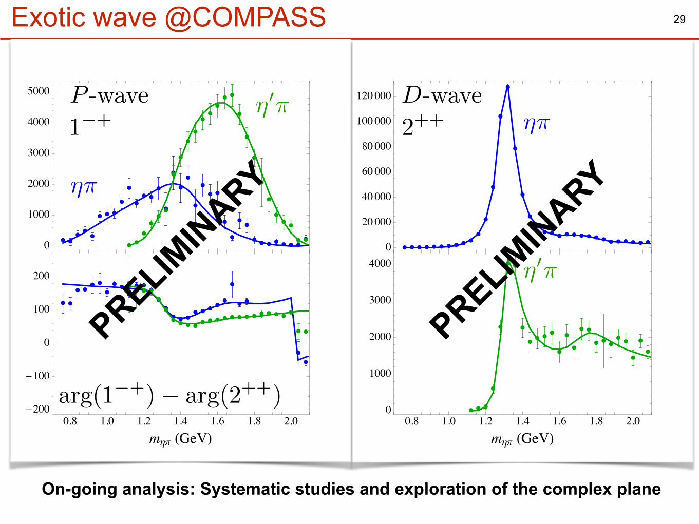
29

P -wave D-wave1�+ 2++

⌘⇡

⌘0⇡

⌘0⇡⌘⇡

PRELIMIN

ARY

PRELIMIN

ARY

Exotic wave @COMPASS

On-going analysis: Systematic studies and exploration of the complex plane

arg(1�+)� arg(2++)

a

b

1

2

3

P

Y⌘

⇡�

⇡�

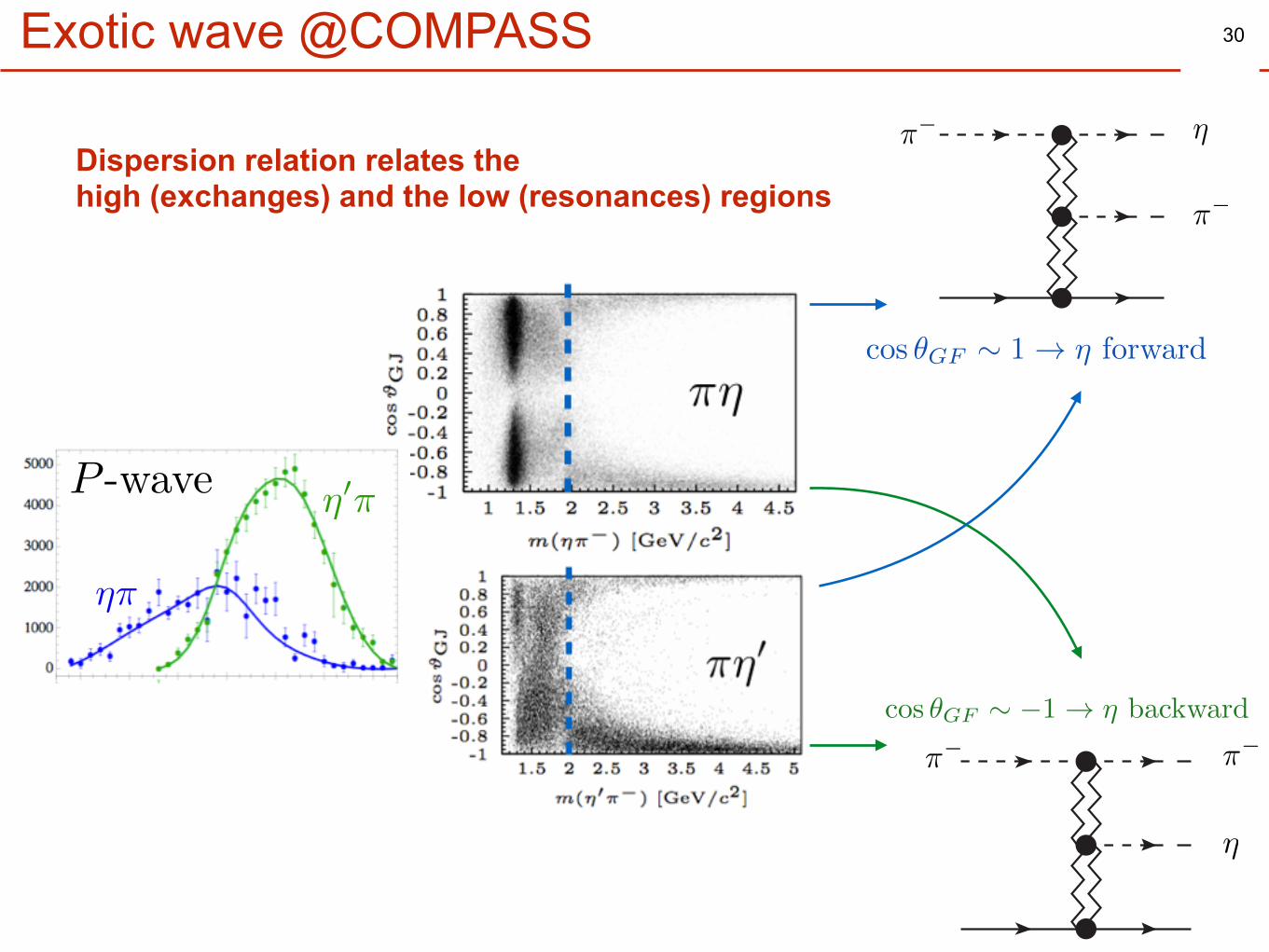
30Exotic wave @COMPASS

a

b

1

2

3

P

Y

⌘

⇡�⇡�

cos ✓GF ⇠ 1 ! ⌘ forward

cos ✓GF ⇠ �1 ! ⌘ backward

⌘⇡

⌘0⇡

Dispersion relation relates the high (exchanges) and the low (resonances) regions

P -wave

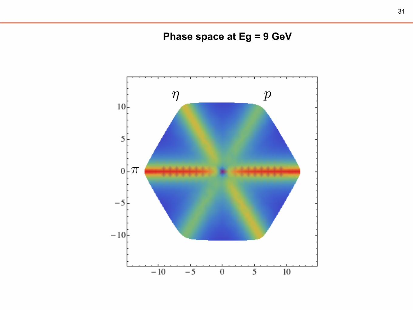
31

⌘

⇡

p

Phase space at Eg = 9 GeV

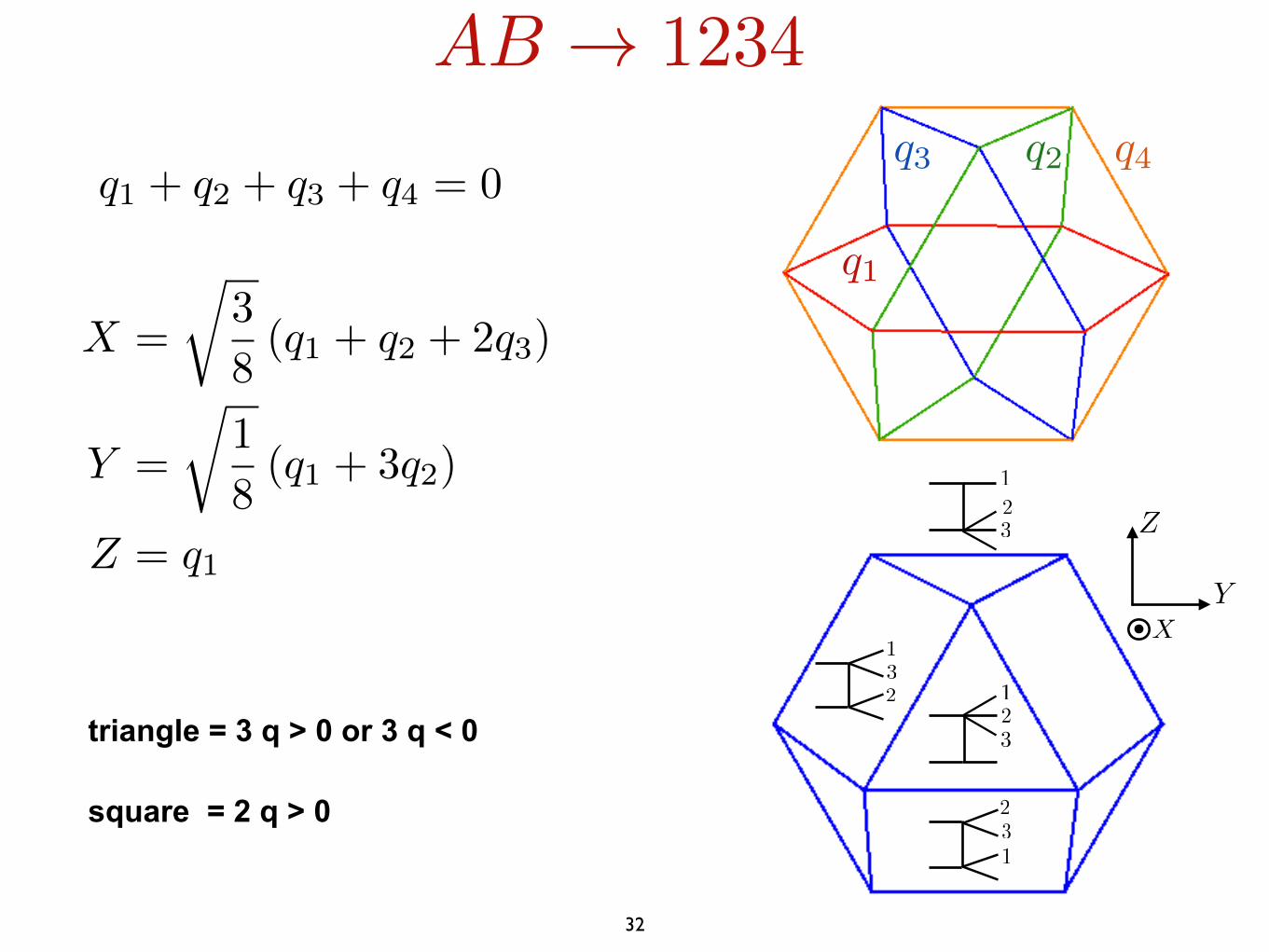
32

X =

r3

8(q1 + q2 + 2q3)

Y =

r1

8(q1 + 3q2)

Z = q1Z

YX

123

123

1

23

1

23

q1 + q2 + q3 + q4 = 0

q1

q2q3 q4

AB ! 1234

triangle = 3 q > 0 or 3 q < 0

square = 2 q > 0

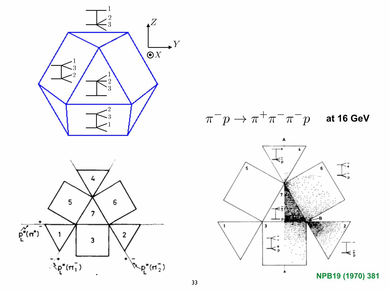
⇡�p ! ⇡+⇡�⇡�p at 16 GeV

33NPB19 (1970) 381

Z

YX

123

123

1

23

1

23

34

Z

YX

123

123

1

23

1

23

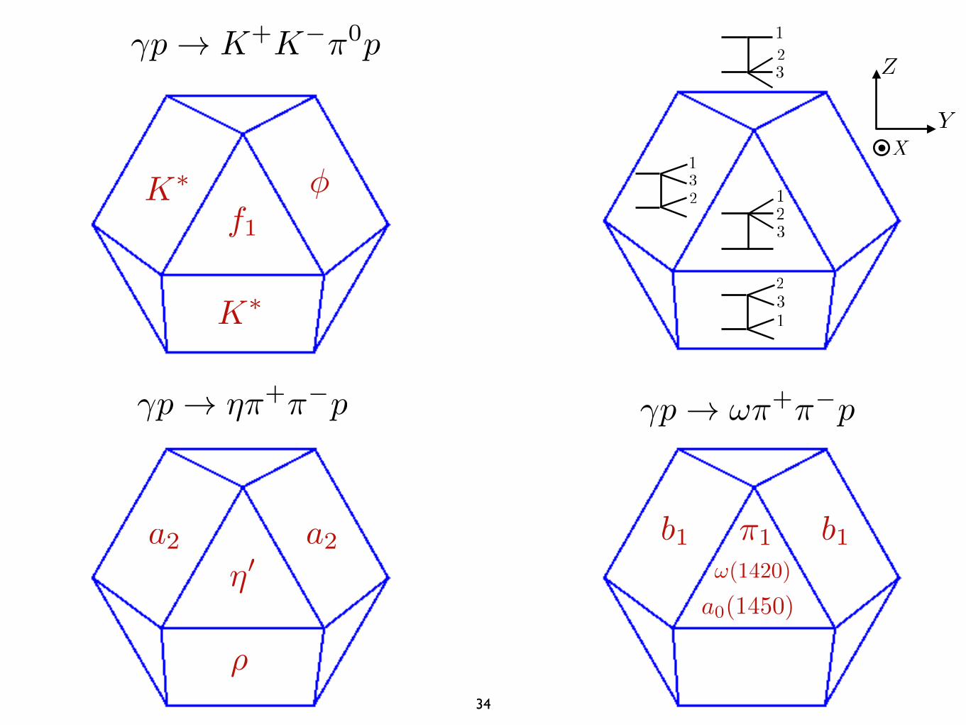
�p ! K+K�⇡0p

�K⇤

K⇤

f1

�p ! ⌘⇡+⇡�p

⌘0

⇢

a2a2

�p ! !⇡+⇡�p

b1 b1!(1420)

a0(1450)

⇡1

Documents

Discovering Exotic Mesons @CLAS12