Embed Size (px)
Citation preview
Discovery of Lagrange multipliersand Lagrange mechanics
– p.1/45
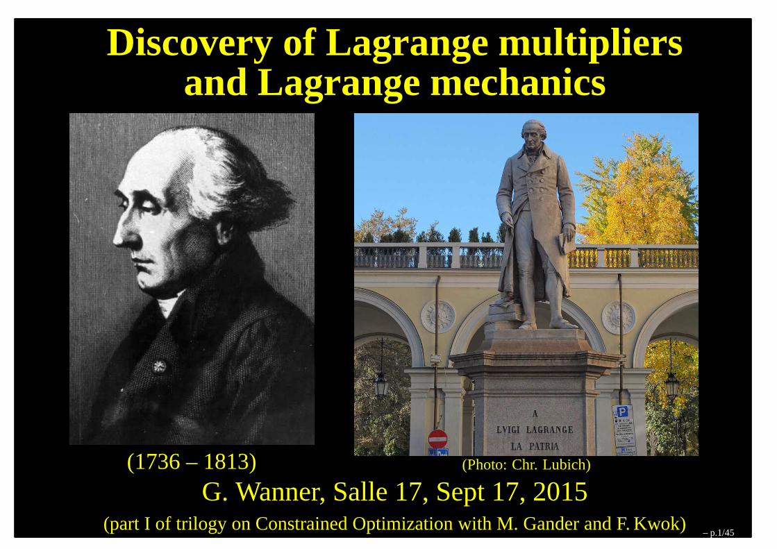
Discovery of Lagrange multipliersand Lagrange mechanics
(1736 – 1813) (Photo: Chr. Lubich)
G. Wanner, Salle 17, Sept 17, 2015(part I of trilogy on Constrained Optimization with M. Gander and F. Kwok)
– p.1/45
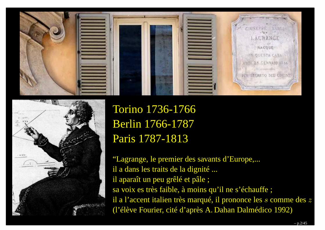
Torino 1736-1766Berlin 1766-1787Paris 1787-1813
“Lagrange, le premier des savants d’Europe,...il a dans les traits de la dignité ...il aparaît un peu grêlé et pâle ;sa voix es très faible, à moins qu’il ne s’échauffe ;il a l’accent italien très marqué, il prononce less comme desz(l’élève Fourier, cité d’après A. Dahan Dalmédico 1992)
– p.2/45
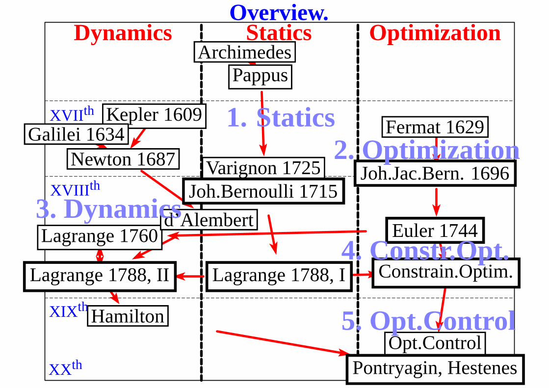
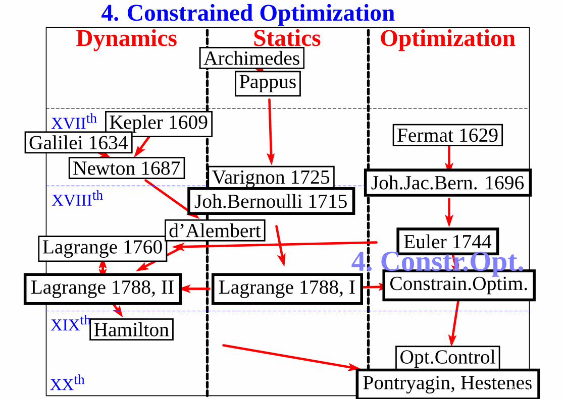
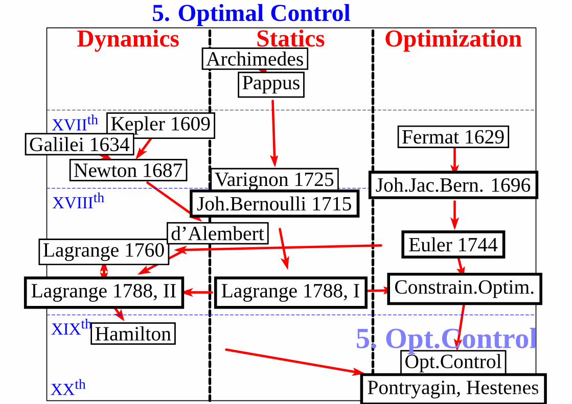
Overview.
ArchimedesArchimedesPappusPappus
Varignon 1725Varignon 1725
Kepler 1609Kepler 1609Galilei 1634Galilei 1634
Newton 1687Newton 1687
Joh.Bernoulli 1715Joh.Bernoulli 1715
Fermat 1629Fermat 1629
Joh.Jac.Bern. 1696Joh.Jac.Bern. 1696
Euler 1744Euler 1744
Constrain.Optim.Constrain.Optim.
Opt.ControlOpt.ControlPontryagin, HestenesPontryagin, Hestenes
Lagrange 1760Lagrange 1760
Lagrange 1788, ILagrange 1788, ILagrange 1788, IILagrange 1788, II
d’Alembertd’Alembert
HamiltonHamilton
StaticsDynamics Optimization
XVII th
XVIII th
XIX th
XX th
1. Statics2. Optimization
3. Dynamics
4. Constr.Opt.
5. Opt.Control
– p.3/45
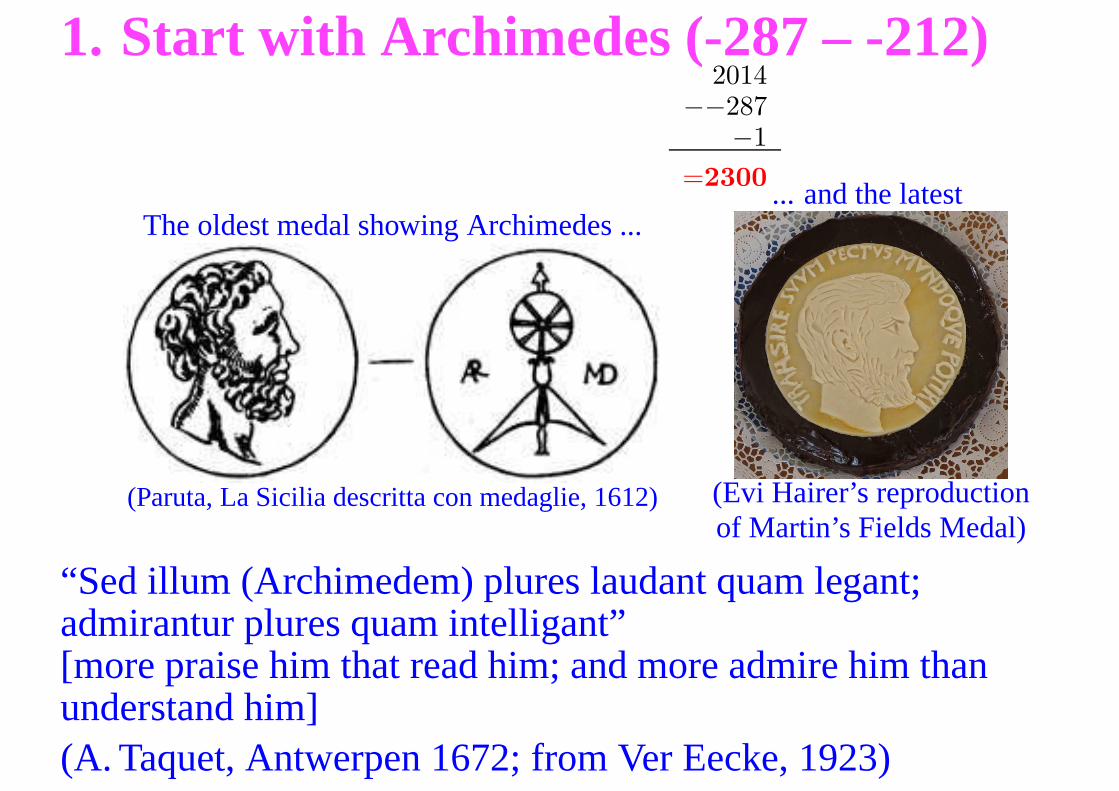
1. Start with Archimedes (-287 – -212)2014
−−287−1
=2300
The oldest medal showing Archimedes ...
(Paruta, La Sicilia descritta con medaglie, 1612)
... and the latest
(Evi Hairer’s reproductionof Martin’s Fields Medal)
“Sed illum (Archimedem) plures laudant quam legant;admirantur plures quam intelligant”[more praise him that read him; and more admire him thanunderstand him](A. Taquet, Antwerpen 1672; from Ver Eecke, 1923) – p.4/45
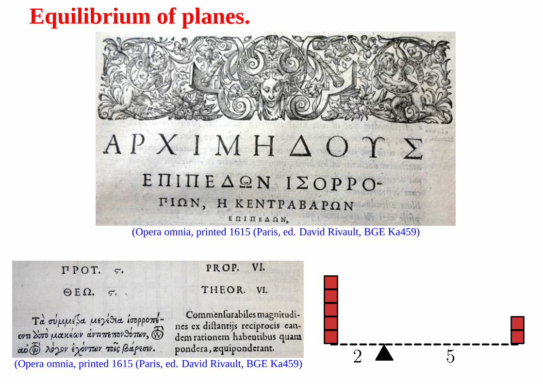
Equilibrium of planes.
(Opera omnia, printed 1615 (Paris, ed. David Rivault, BGE Ka459)
(Opera omnia, printed 1615 (Paris, ed. David Rivault, BGE Ka459) 2 5– p.5/45
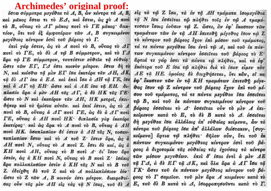
Archimedes’ original proof:
– p.6/45
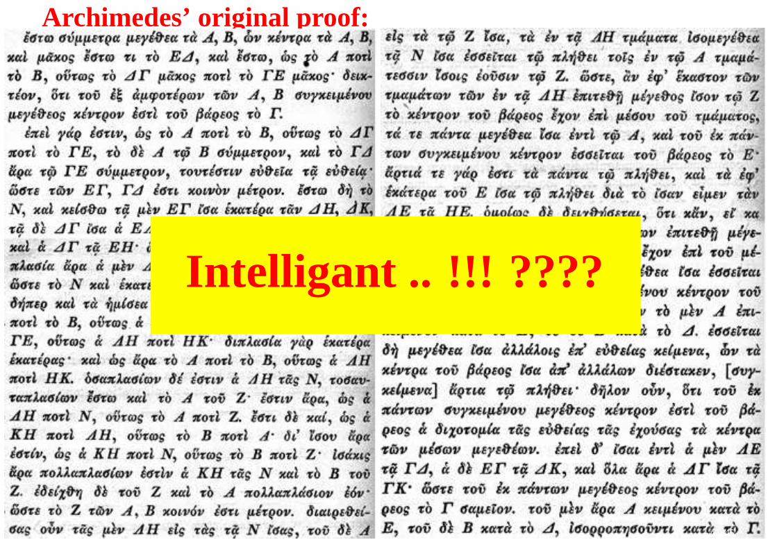
Archimedes’ original proof:
Intelligant .. !!! ????
– p.6/45
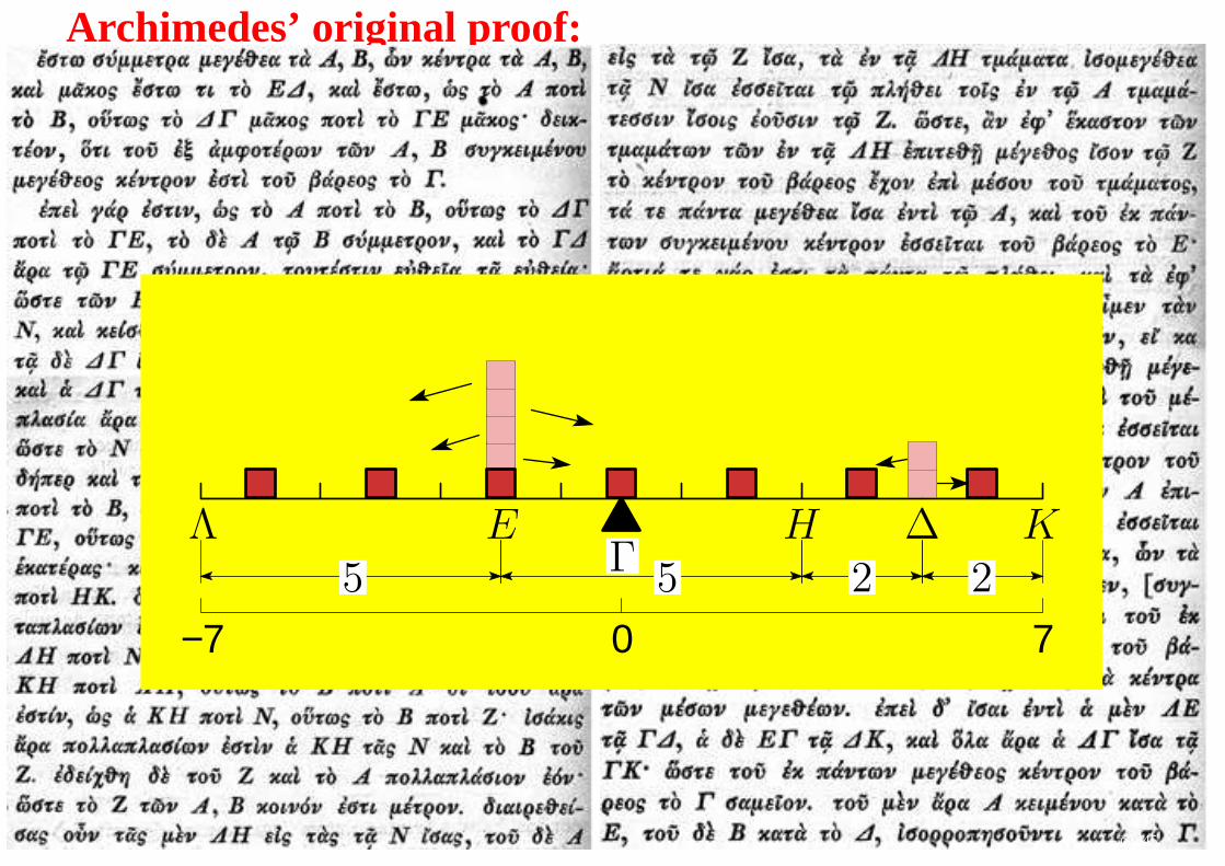
Archimedes’ original proof:
Intelligant .. !!! ????
−7 0 75 5 2 2
Λ EΓ
H ∆ K
– p.6/45
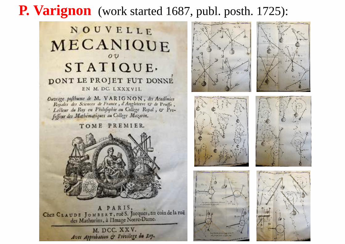
P. Varignon (work started 1687, publ. posth. 1725):
– p.7/45
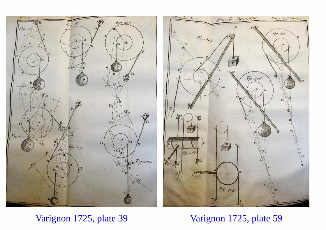
Varignon 1725, plate 39 Varignon 1725, plate 59– p.8/45
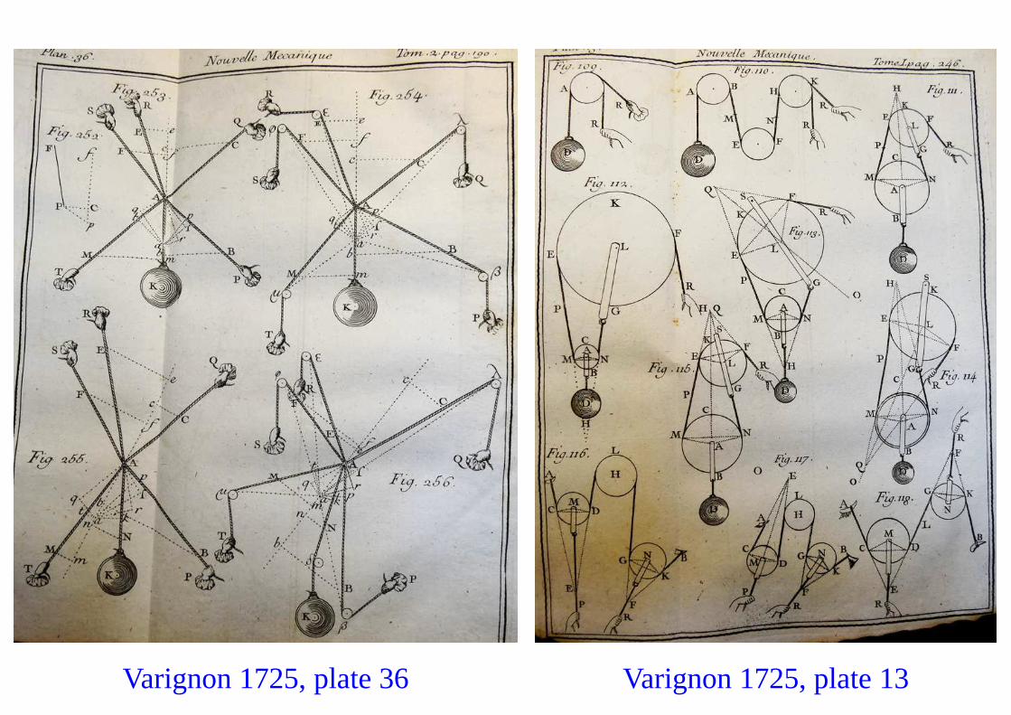
Varignon 1725, plate 36 Varignon 1725, plate 13– p.9/45
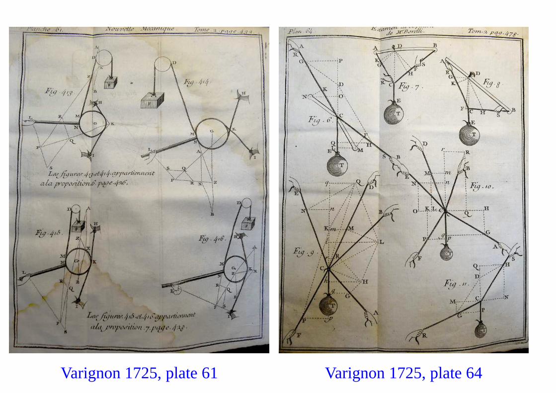
Varignon 1725, plate 61 Varignon 1725, plate 64– p.10/45
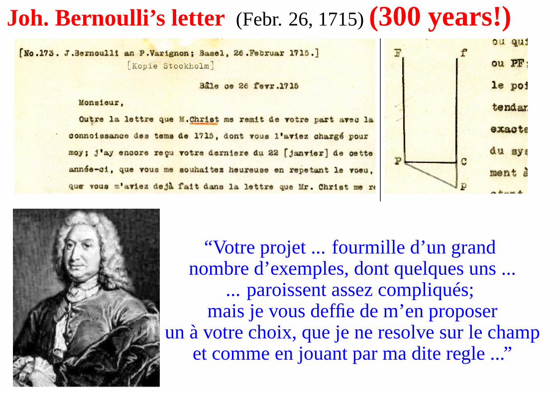
Joh. Bernoulli’s letter (Febr. 26, 1715)(300 years!)
“Votre projet ... fourmille d’un grandnombre d’exemples, dont quelques uns ...
... paroissent assez compliqués;mais je vous deffie de m’en proposer
un à votre choix, que je ne resolve sur le champet comme en jouant par ma dite regle ...”
– p.11/45
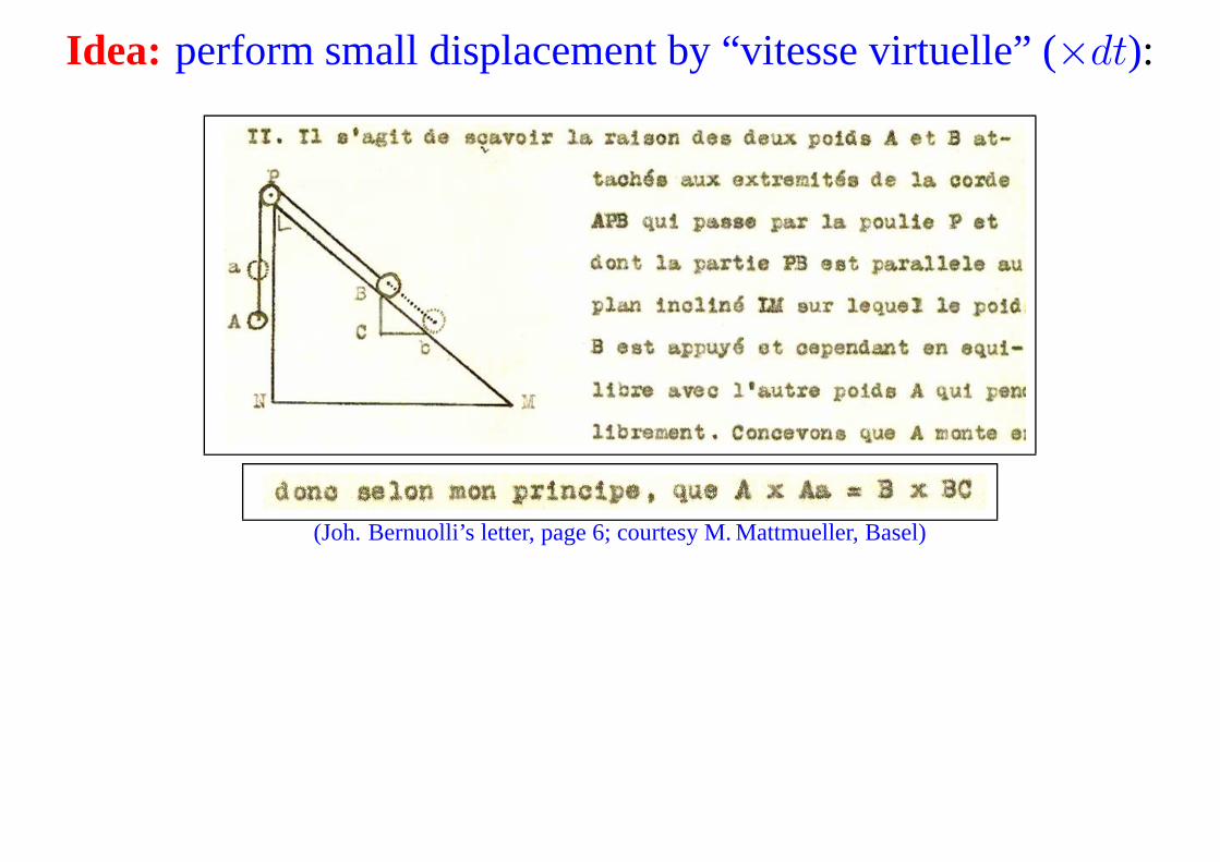
Idea: perform small displacement by “vitesse virtuelle” (×dt):
(Joh. Bernuolli’s letter, page 6; courtesy M. Mattmueller,Basel)
– p.12/45
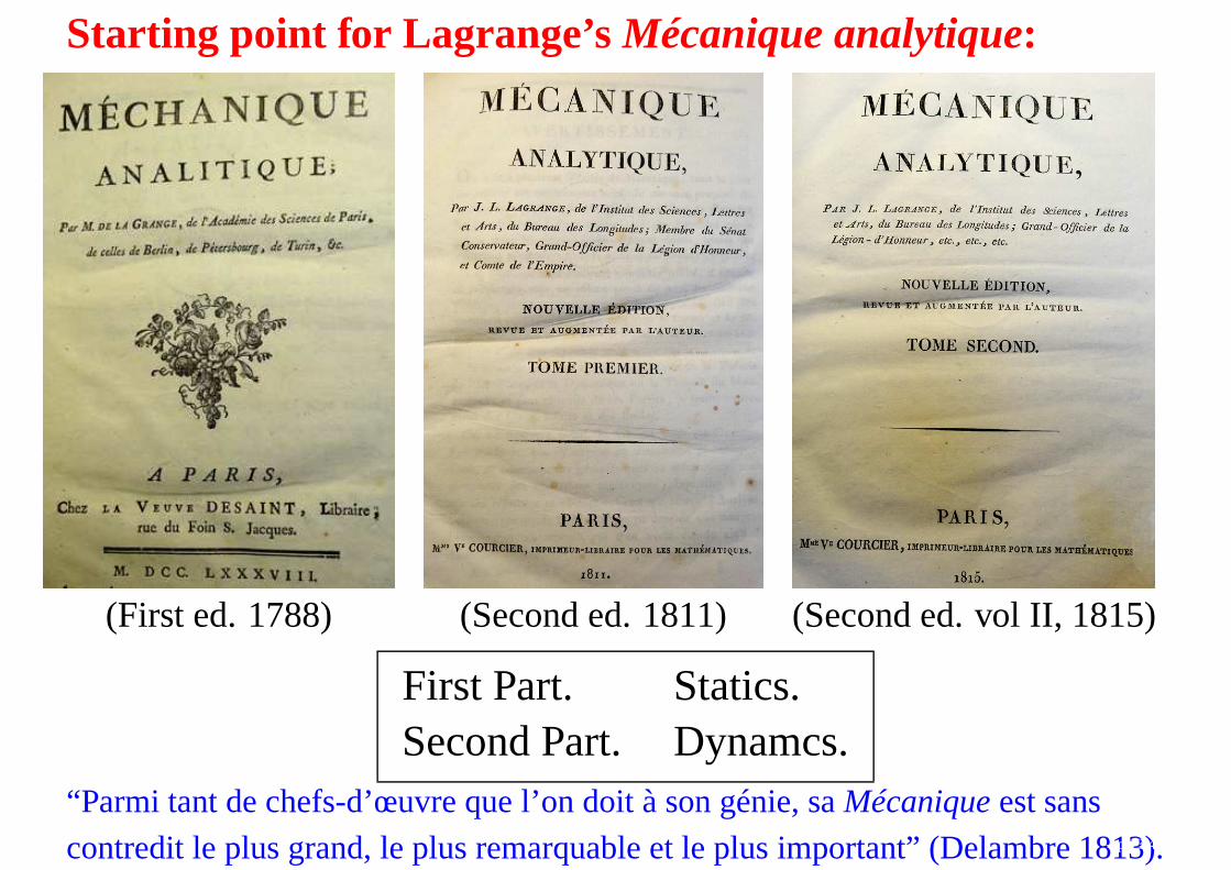
Starting point for Lagrange’s Mécanique analytique:
(First ed. 1788) (Second ed. 1811) (Second ed. vol II, 1815)
First Part. Statics.Second Part. Dynamcs.
“Parmi tant de chefs-d’œuvre que l’on doit à son génie, saMécaniqueest sans
contredit le plus grand, le plus remarquable et le plus important” (Delambre 1813).– p.13/45
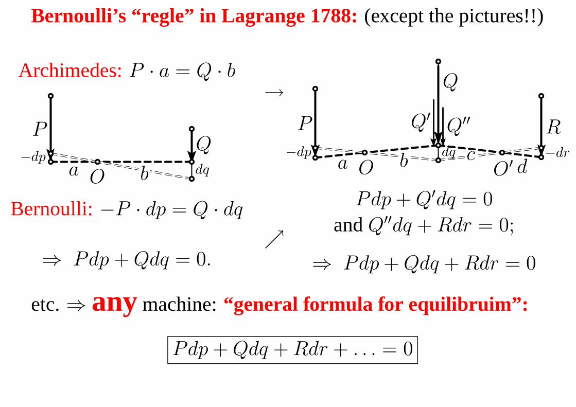
Bernoulli’s “regle” in Lagrange 1788: (except the pictures!!)
Archimedes:P · a = Q · b
a b−dp
dq
PQ
O
Bernoulli: −P · dp = Q · dq
⇒ Pdp + Qdq = 0.
→
ր
a b cd
−dp dq −dr
P
Q
Q′Q′′ R
O O′
Pdp + Q′dq = 0
andQ′′dq + Rdr = 0;
⇒ Pdp + Qdq + Rdr = 0
etc.⇒ anymachine:“general formula for equilibruim”:
Pdp + Qdq + Rdr + . . . = 0
– p.14/45
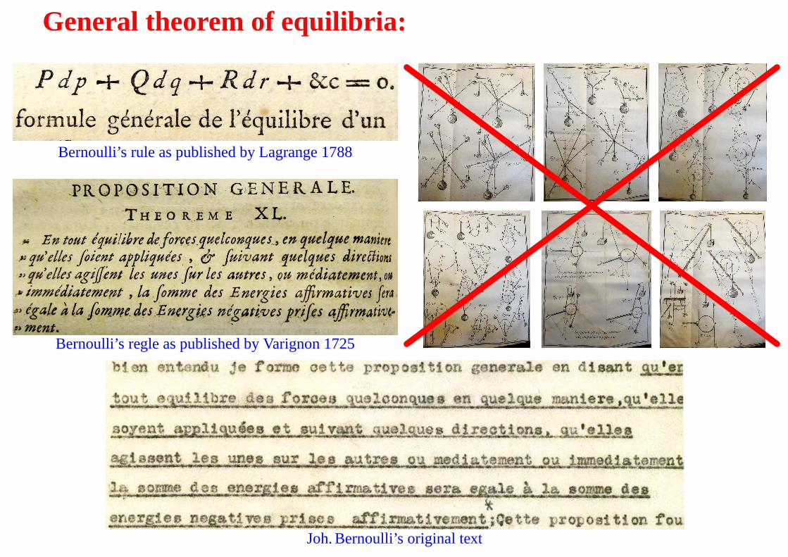
General theorem of equilibria:
Bernoulli’s rule as published by Lagrange 1788
Bernoulli’s regle as published by Varignon 1725
Joh. Bernoulli’s original text – p.15/45
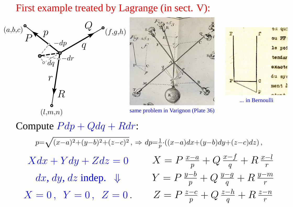
First example treated by Lagrange (in sect. V):
p
q
r
P
Q
R
−dp
dq−dr
(a,b,c) (f,g,h)
(l,m,n) same problem in Varignon (Plate 36)
... in Bernoulli
ComputePdp + Qdq + Rdr:
p=√
(x−a)2+(y−b)2+(z−c)2 , ⇒ dp= 1
p·((x−a)dx+(y−b)dy+(z−c)dz) ,
Xdx + Y dy + Zdz = 0
dx, dy, dz indep. ⇓X = 0 , Y = 0 , Z = 0 .
X = P x−ap
+ Q x−fq
+ R x−lr
Y = P y−bp
+ Q y−gq
+ R y−mr
Z = P z−cp
+ Q z−hq
+ R z−nr– p.16/45
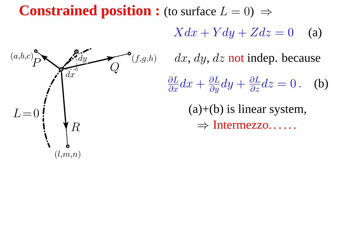
Constrained position : (to surfaceL = 0) ⇒
P Q
R
dx
dy(a,b,c) (f,g,h)
(l,m,n)
L=0
Xdx + Y dy + Zdz = 0 (a)
dx, dy, dz not indep. because
∂L∂x
dx + ∂L∂y
dy + ∂L∂z
dz = 0 . (b)
(a)+(b) is linear system,⇒ Intermezzo. . . . . .
– p.17/45
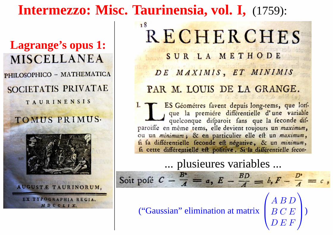
Intermezzo: Misc. Taurinensia, vol. I, (1759):
Lagrange’s opus 1:
... plusieures variables ...
(“Gaussian” elimination at matrix
A B D
B C E
D E F
)
– p.18/45
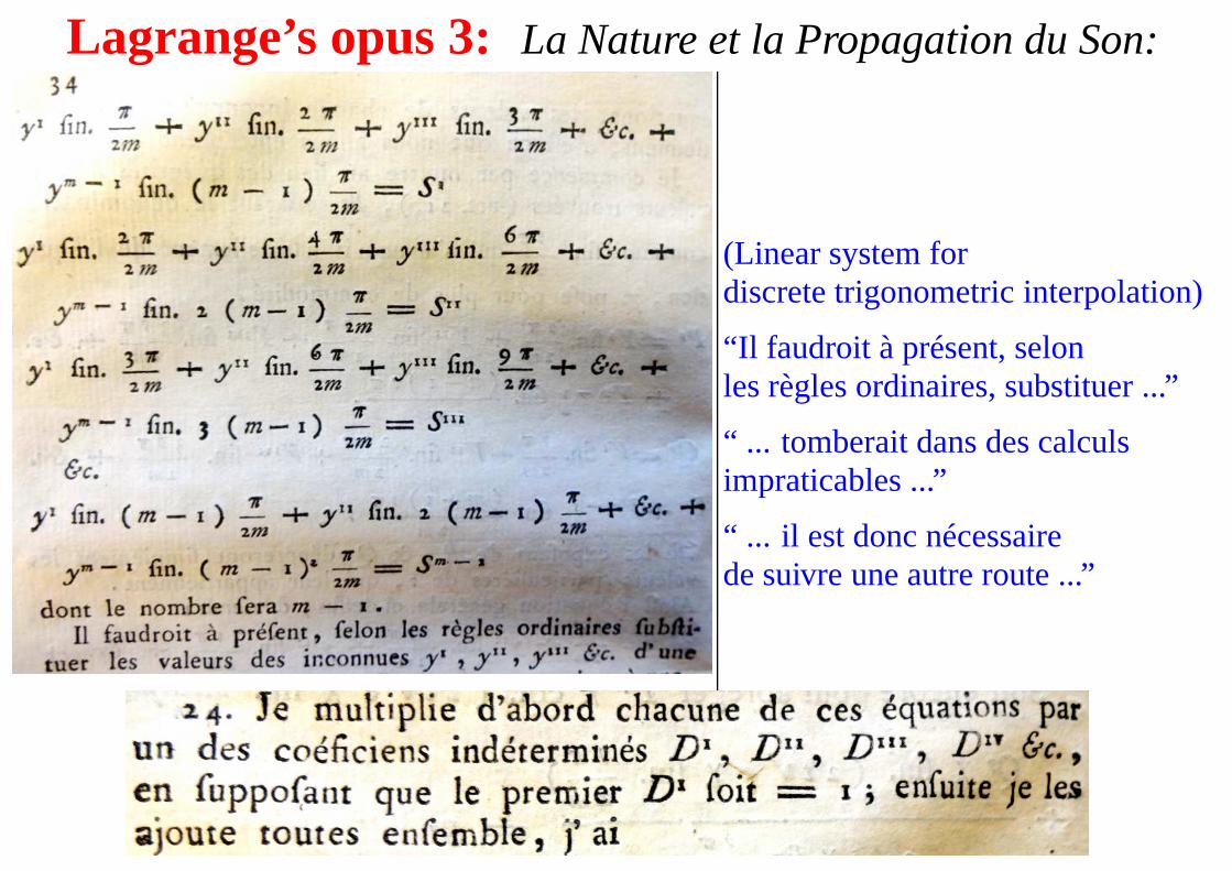
Lagrange’s opus 3: La Nature et la Propagation du Son:
(Linear system fordiscrete trigonometric interpolation)
“Il faudroit à présent, selonles règles ordinaires, substituer ...”
“ ... tomberait dans des calculsimpraticables ...”
“ ... il est donc nécessairede suivre une autre route ...”
– p.19/45
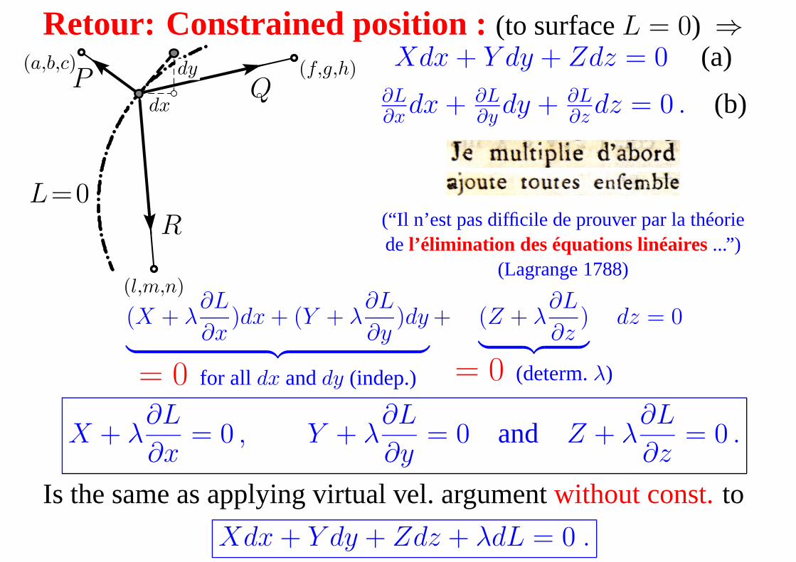
Retour: Constrained position : (to surfaceL = 0) ⇒
P Q
R
dx
dy(a,b,c) (f,g,h)
(l,m,n)
L=0
Xdx + Y dy + Zdz = 0 (a)∂L∂x
dx + ∂L∂y
dy + ∂L∂z
dz = 0 . (b)
(“Il n’est pas difficile de prouver par la théoriede l’élimination des équations linéaires...”)
(Lagrange 1788)
(X + λ∂L
∂x)dx + (Y + λ
∂L
∂y)dy
︸ ︷︷ ︸
= 0 for all dx anddy (indep.)
+ (Z + λ∂L
∂z)
︸ ︷︷ ︸
= 0 (determ.λ)
dz = 0
X + λ∂L
∂x= 0 , Y + λ
∂L
∂y= 0 and Z + λ
∂L
∂z= 0 .
Is the same as applying virtual vel. argumentwithout const.to
Xdx + Y dy + Zdz + λdL = 0 . – p.20/45
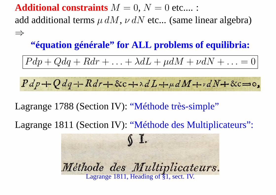
Additional constraints M = 0, N = 0 etc.... :add additional termsµ dM , ν dN etc... (same linear algebra)⇒
“équation générale” for ALL problems of equilibria:
Pdp + Qdq + Rdr + . . . + λdL + µdM + νdN + . . . = 0
Lagrange 1788 (Section IV):“Méthode très-simple”
Lagrange 1811 (Section IV):“Méthode des Multiplicateurs”:
Lagrange 1811, Heading of §1, sect. IV.
– p.21/45
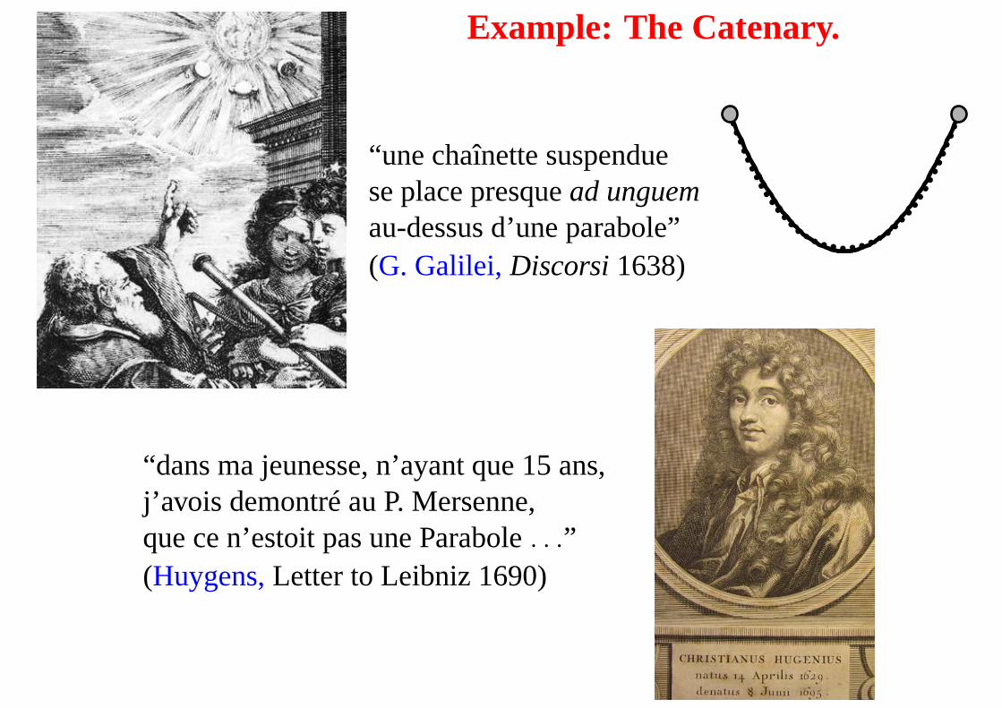
Example: The Catenary.
“une chaînette suspenduese place presquead unguemau-dessus d’une parabole”(G. Galilei,Discorsi1638)
“dans ma jeunesse, n’ayant que 15 ans,j’avois demontré au P. Mersenne,que ce n’estoit pas une Parabole. . .”(Huygens,Letter to Leibniz 1690)
– p.22/45
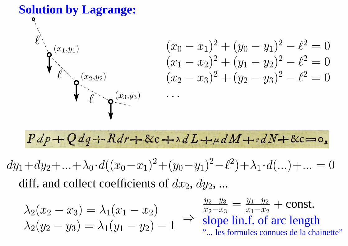
Solution by Lagrange:
ℓ
ℓ
ℓ
(x1,y1)
(x2,y2)
(x3,y3)
(x0 − x1)2 + (y0 − y1)
2 − ℓ2 = 0
(x1 − x2)2 + (y1 − y2)
2 − ℓ2 = 0
(x2 − x3)2 + (y2 − y3)
2 − ℓ2 = 0
. . .
dy1+dy2+...+λ0 ·d((x0−x1)2+(y0−y1)
2−ℓ2)+λ1 ·d(...)+... = 0
diff. and collect coefficients ofdx2, dy2, ...
λ2(x2 − x3) = λ1(x1 − x2)
λ2(y2 − y3) = λ1(y1 − y2) − 1⇒
y2−y3
x2−x3
= y1−y2
x1−x2
+ const.slope lin.f. of arc length”... les formules connues de la chainette”
– p.23/45
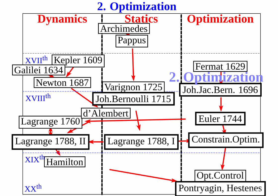
2. Optimization
ArchimedesArchimedesPappusPappus
Varignon 1725Varignon 1725
Kepler 1609Kepler 1609Galilei 1634Galilei 1634
Newton 1687Newton 1687
Joh.Bernoulli 1715Joh.Bernoulli 1715
Fermat 1629Fermat 1629
Joh.Jac.Bern. 1696Joh.Jac.Bern. 1696
Euler 1744Euler 1744
Constrain.Optim.Constrain.Optim.
Opt.ControlOpt.ControlPontryagin, HestenesPontryagin, Hestenes
Lagrange 1760Lagrange 1760
Lagrange 1788, ILagrange 1788, ILagrange 1788, IILagrange 1788, II
d’Alembertd’Alembert
HamiltonHamilton
StaticsDynamics Optimization
XVII th
XVIII th
XIX th
XX th
2. Optimization
– p.24/45
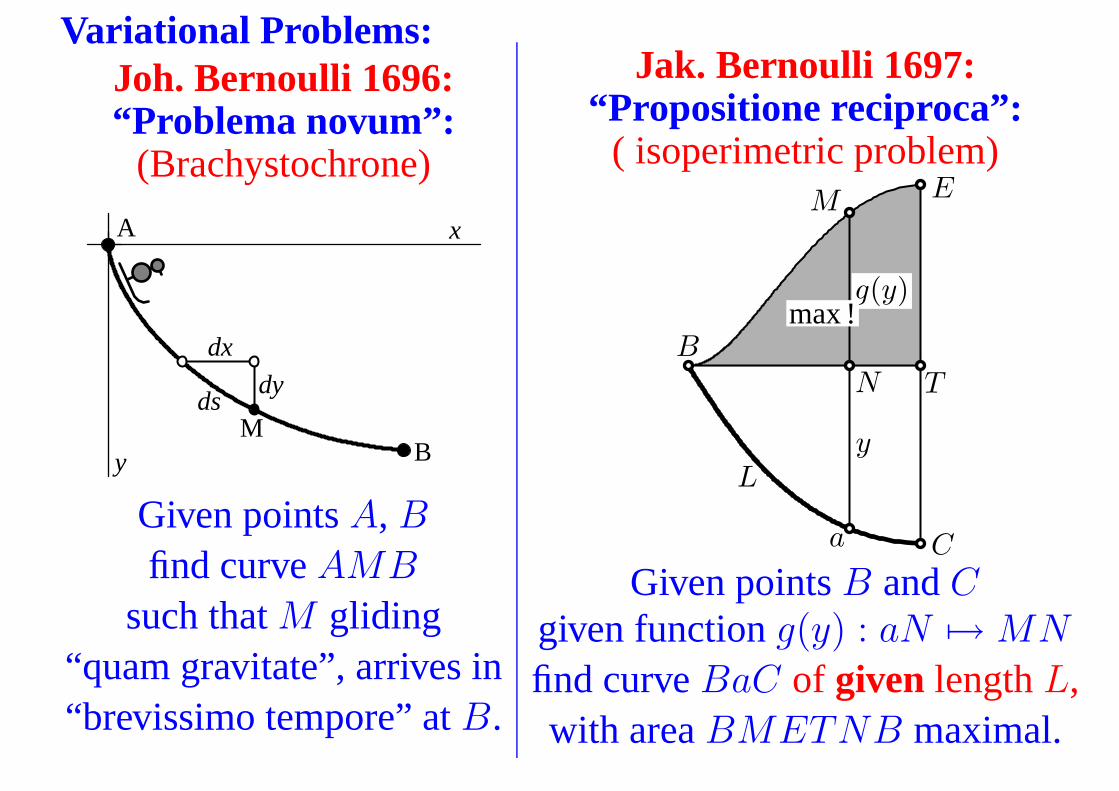
Variational Problems:Joh. Bernoulli 1696:“Problema novum”:
(Brachystochrone)
dxdx
dydydsds
A
BM
x
y
Given pointsA, B
find curveAMB
such thatM gliding“quam gravitate”, arrives in“brevissimo tempore” atB.
Jak. Bernoulli 1697:“Propositione reciproca”:
( isoperimetric problem)
y
g(y)max !
L
B
C
E
T
a
M
N
Given pointsB andC
given functiong(y) : aN 7→ MN
find curveBaC of given lengthL,with areaBMETNB maximal.
– p.25/45
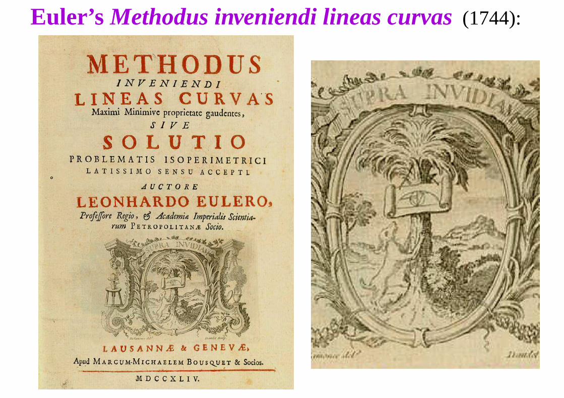
Euler’s Methodus inveniendi lineas curvas(1744):
– p.26/45
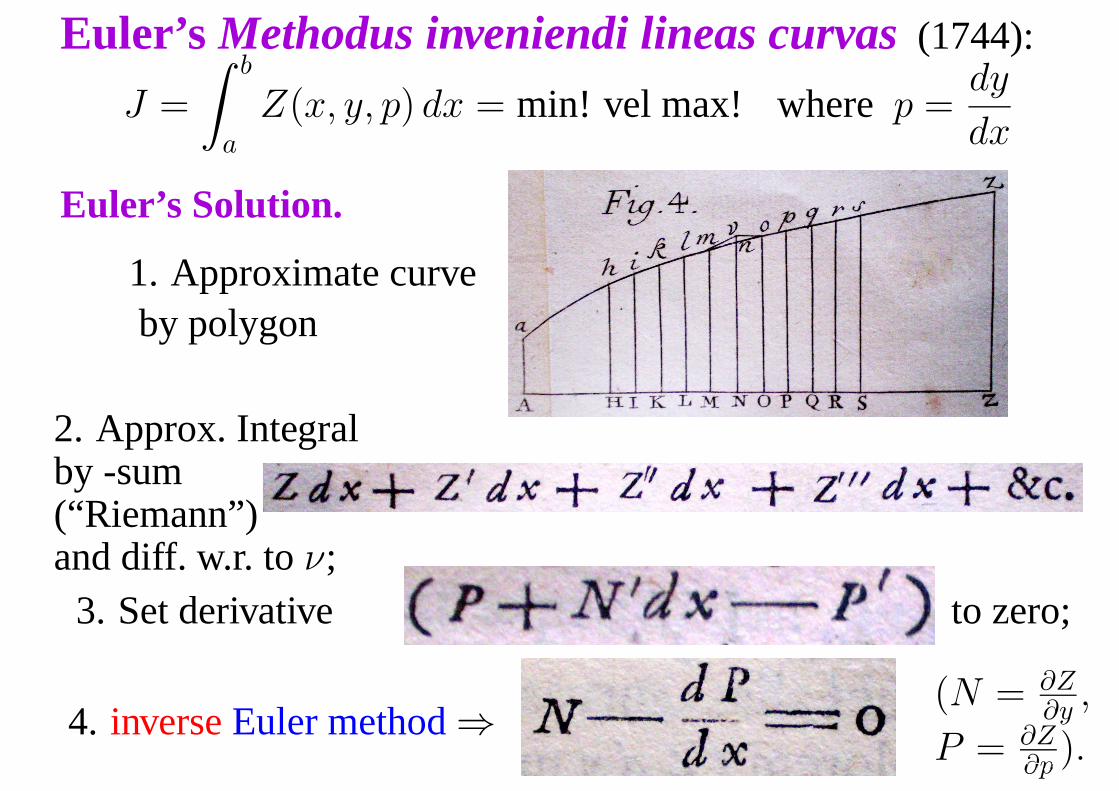
Euler’s Methodus inveniendi lineas curvas(1744):
J =
∫ b
a
Z(x, y, p) dx = min! vel max! wherep =dy
dx
Euler’s Solution.
1. Approximate curveby polygon
2. Approx. Integralby -sum(“Riemann”)and diff. w.r. toν;
3. Set derivative to zero;
4. inverseEuler method⇒ (N = ∂Z∂y
,
P = ∂Z∂p
).– p.27/45
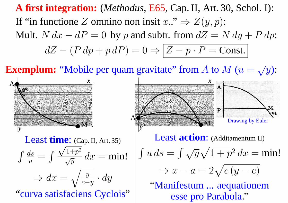
A first integration: (Methodus, E65, Cap. II, Art. 30, Schol. I):If “in functione Z omnino non insitx..” ⇒ Z(y, p):Mult. N dx − dP = 0 by p and subtr. fromdZ = N dy + P dp:
dZ − (P dp + p dP ) = 0 ⇒ Z − p · P = Const.
Exemplum: “Mobile per quam gravitate” fromA to M (u =√
y):A
M
x
y
AM
x
yDrawing by Euler
Leasttime: (Cap. II, Art. 35)∫
dsu
=∫√
1+p2
√y
dx = min!
⇒ dx =√
yc−y
· dy
“curva satisfaciens Cyclois”
Leastaction: (Additamentum II)∫
u ds =∫ √
y√
1 + p2 dx = min!
⇒ x − a = 2√
c (y − c)
“Manifestum ... aequationemesse pro Parabola.” – p.28/45
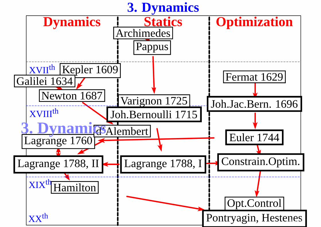
3. Dynamics
ArchimedesArchimedesPappusPappus
Varignon 1725Varignon 1725
Kepler 1609Kepler 1609Galilei 1634Galilei 1634
Newton 1687Newton 1687
Joh.Bernoulli 1715Joh.Bernoulli 1715
Fermat 1629Fermat 1629
Joh.Jac.Bern. 1696Joh.Jac.Bern. 1696
Euler 1744Euler 1744
Constrain.Optim.Constrain.Optim.
Opt.ControlOpt.ControlPontryagin, HestenesPontryagin, Hestenes
Lagrange 1760Lagrange 1760
Lagrange 1788, ILagrange 1788, ILagrange 1788, IILagrange 1788, II
d’Alembertd’Alembert
HamiltonHamilton
StaticsDynamics Optimization
XVII th
XVIII th
XIX th
XX th
3. Dynamics
– p.29/45
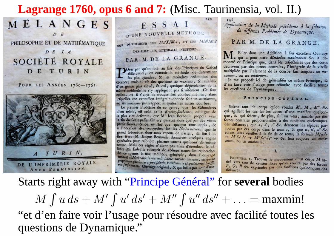
Lagrange 1760, opus 6 and 7:(Misc. Taurinensia, vol. II.)
Starts right away with “Principe Général”for severalbodies
M∫
u ds + M ′ ∫ u′ ds′ + M ′′ ∫ u′′ ds′′ + . . . = maxmin!“et d’en faire voir l’usage pour résoudre avec facilité toutes lesquestions de Dynamique.” – p.30/45
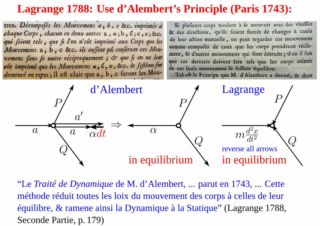
Lagrange 1788: Use d’Alembert’s Principle (Paris 1743):
P
Q
aa′
a αdt⇒
d’AlembertP
Qα
in equilibrium
P
Qmd2x
dt2
Lagrange
in equilibriumreverse all arrows
“Le Traité de Dynamiquede M. d’Alembert, ... parut en 1743, ... Cetteméthode réduit toutes les loix du mouvement des corps à celles de leuréquilibre, & ramene ainsi la Dynamique à la Statique”(Lagrange 1788,Seconde Partie, p. 179) – p.31/45
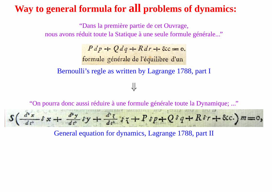
Way to general formula for all problems of dynamics:
“Dans la première partie de cet Ouvrage,nous avons réduit toute la Statique à une seule formule générale...”
Bernoulli’s regle as written by Lagrange 1788, part I
⇓“On pourra donc aussi réduire à une formule générale toute laDynamique; ...”
General equation for dynamics, Lagrange 1788, part II
– p.32/45
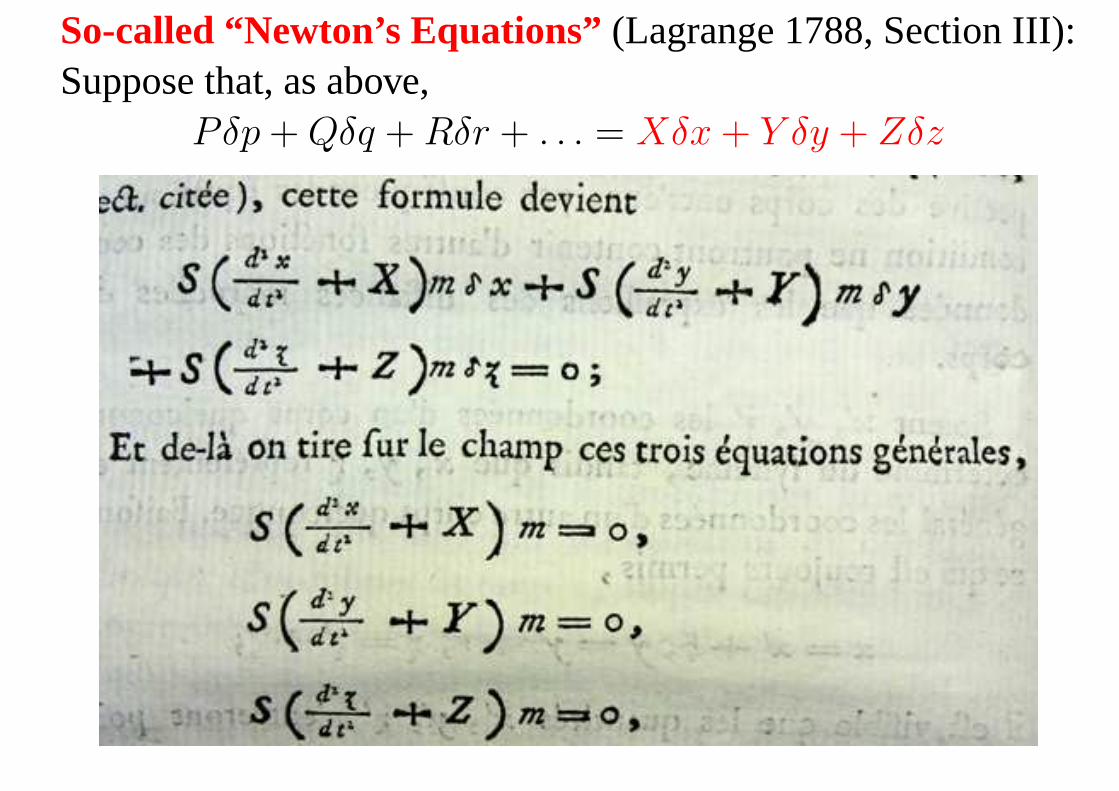
So-called “Newton’s Equations”(Lagrange 1788, Section III):Suppose that, as above,
Pδp + Qδq + Rδr + . . . = Xδx + Y δy + Zδz
– p.33/45
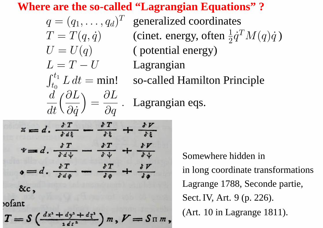
Where are the so-called “Lagrangian Equations” ?q = (q1, . . . , qd)
T generalized coordinatesT = T (q, q) (cinet. energy, often12 q
TM(q)q )U = U(q) ( potential energy)L = T − U Lagrangian∫ t1
t0Ldt = min! so-called Hamilton Principle
d
dt
(∂L
∂q
)
=∂L
∂q. Lagrangian eqs.
Somewhere hidden in
in long coordinate transformations
Lagrange 1788, Seconde partie,
Sect. IV, Art. 9 (p. 226).
(Art. 10 in Lagrange 1811).– p.34/45
4. Constrained Optimization
ArchimedesArchimedesPappusPappus
Varignon 1725Varignon 1725
Kepler 1609Kepler 1609Galilei 1634Galilei 1634
Newton 1687Newton 1687
Joh.Bernoulli 1715Joh.Bernoulli 1715
Fermat 1629Fermat 1629
Joh.Jac.Bern. 1696Joh.Jac.Bern. 1696
Euler 1744Euler 1744
Constrain.Optim.Constrain.Optim.
Opt.ControlOpt.ControlPontryagin, HestenesPontryagin, Hestenes
Lagrange 1760Lagrange 1760
Lagrange 1788, ILagrange 1788, ILagrange 1788, IILagrange 1788, II
d’Alembertd’Alembert
HamiltonHamilton
StaticsDynamics Optimization
XVII th
XVIII th
XIX th
XX th
4. Constr.Opt.
– p.35/45
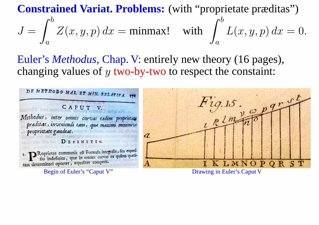
Constrained Variat. Problems: (with “proprietate præditas”)
J =
∫ b
a
Z(x, y, p) dx = minmax! with∫ b
a
L(x, y, p) dx = 0.
Euler’sMethodus, Chap. V:entirely new theory (16 pages),changing values ofy two-by-twoto respect the constaint:
Begin of Euler’s “Caput V” Drawing in Euler’s Caput V
– p.36/45
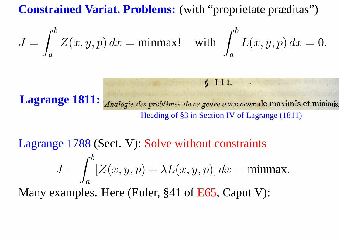
Constrained Variat. Problems: (with “proprietate præditas”)
J =
∫ b
a
Z(x, y, p) dx = minmax! with∫ b
a
L(x, y, p) dx = 0.
Lagrange 1811:Heading of §3 in Section IV of Lagrange (1811)
Lagrange 1788(Sect. V):Solve without constraints
J =
∫ b
a
[Z(x, y, p) + λL(x, y, p)] dx = minmax.
Many examples. Here (Euler, §41 ofE65, Caput V):
– p.37/45
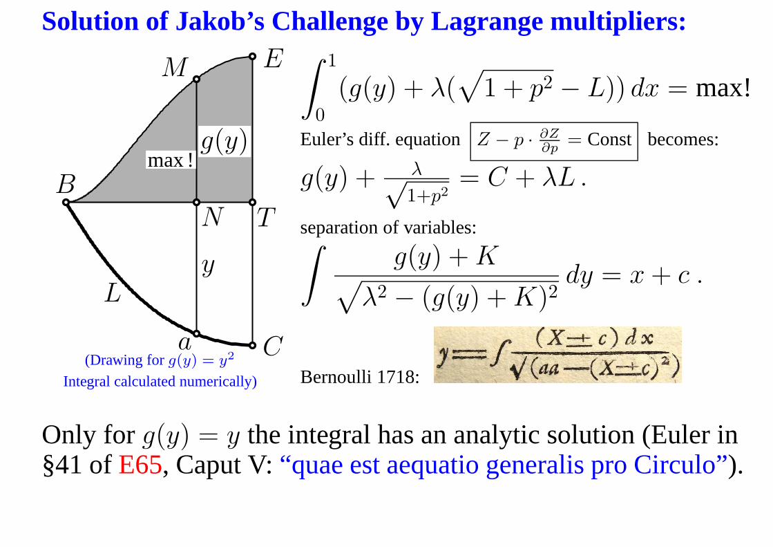
Solution of Jakob’s Challenge by Lagrange multipliers:
y
g(y)max !
L
B
C
E
T
a
M
N
(Drawing forg(y) = y2
Integral calculated numerically)
∫ 1
0
(g(y) + λ(√
1 + p2 − L)) dx = max!
Euler’s diff. equation Z − p · ∂Z∂p
= Const becomes:
g(y) + λ√1+p2
= C + λL .
separation of variables:∫
g(y) + K√
λ2 − (g(y) + K)2dy = x + c .
Bernoulli 1718:
Only for g(y) = y the integral has an analytic solution (Euler in§41 ofE65, Caput V:“quae est aequatio generalis pro Circulo”).
– p.38/45
5. Optimal Control
ArchimedesArchimedesPappusPappus
Varignon 1725Varignon 1725
Kepler 1609Kepler 1609Galilei 1634Galilei 1634
Newton 1687Newton 1687
Joh.Bernoulli 1715Joh.Bernoulli 1715
Fermat 1629Fermat 1629
Joh.Jac.Bern. 1696Joh.Jac.Bern. 1696
Euler 1744Euler 1744
Constrain.Optim.Constrain.Optim.
Opt.ControlOpt.ControlPontryagin, HestenesPontryagin, Hestenes
Lagrange 1760Lagrange 1760
Lagrange 1788, ILagrange 1788, ILagrange 1788, IILagrange 1788, II
d’Alembertd’Alembert
HamiltonHamilton
StaticsDynamics Optimization
XVII th
XVIII th
XIX th
XX th
5. Opt.Control
– p.39/45
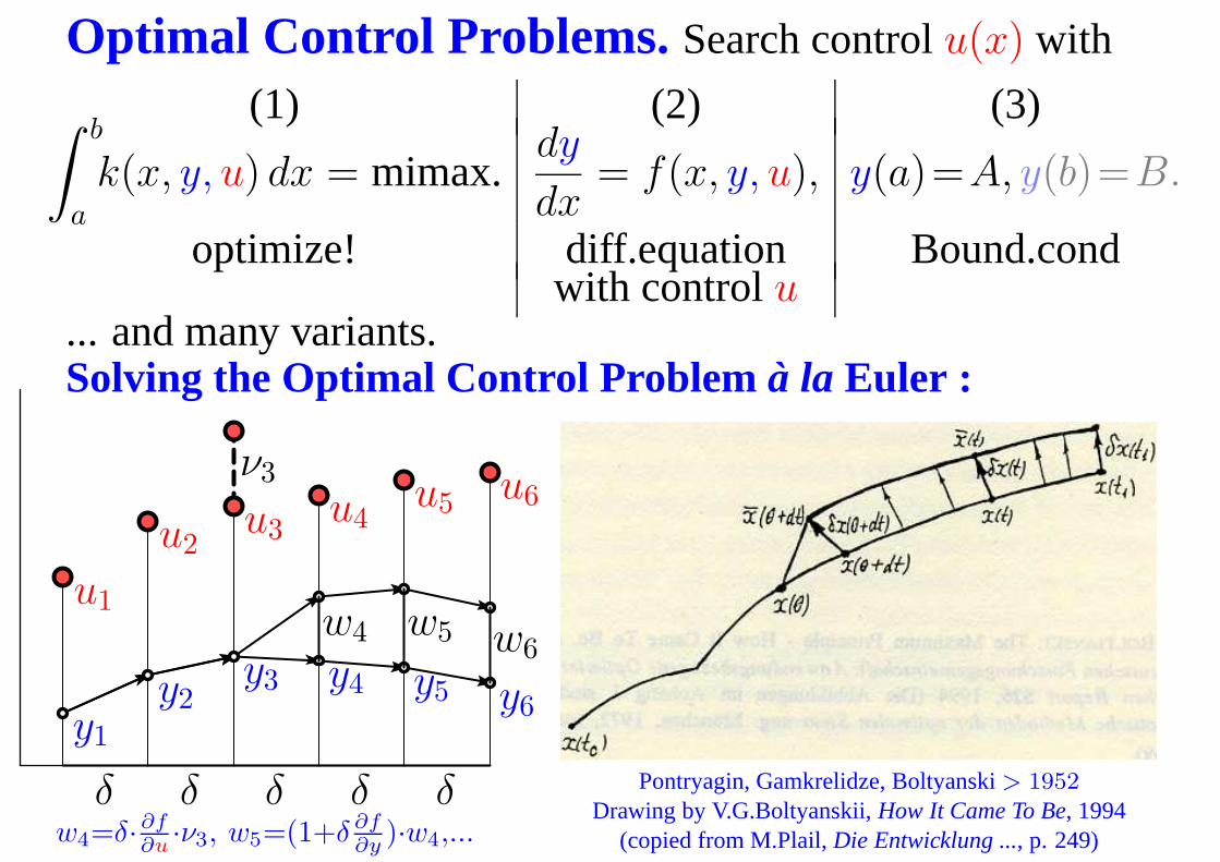
Optimal Control Problems. Search controlu(x) with
(1) (2) (3)∫ b
a
k(x, y, u) dx = mimax.dy
dx= f(x, y, u), y(a)=A, y(b)=B.
optimize! diff.equation Bound.condwith controlu
... and many variants.Solving the Optimal Control Problem à la Euler :
δ δ δ δ δ
y1
y2y3 y4 y5 y6
u1
u2u3
u4u5 u6
w4 w5 w6
ν3
w4=δ·∂f∂u
·ν3, w5=(1+δ ∂f∂y
)·w4,...
Optimal controlà la Euler
Pontryagin, Gamkrelidze, Boltyanski> 1952Drawing by V.G.Boltyanskii,How It Came To Be, 1994
(copied from M.Plail,Die Entwicklung ..., p. 249)– p.40/45
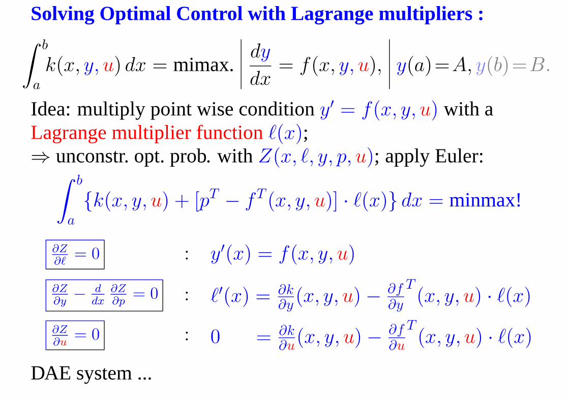
Solving Optimal Control with Lagrange multipliers :∫ b
a
k(x, y, u) dx = mimax.dy
dx= f(x, y, u), y(a)=A, y(b)=B.
Idea: multiply point wise conditiony′ = f(x, y, u) with aLagrange multiplier functionℓ(x);⇒ unconstr. opt. prob. withZ(x, ℓ, y, p, u); apply Euler:
∫ b
a
{k(x, y, u) + [pT − fT (x, y, u)] · ℓ(x)} dx = minmax!
∂Z∂ℓ
= 0 : y′(x) = f(x, y, u)
∂Z∂y
− ddx
∂Z∂p
= 0 : ℓ′(x) = ∂k∂y
(x, y, u) − ∂f∂y
T(x, y, u) · ℓ(x)
∂Z∂u
= 0 : 0 = ∂k∂u
(x, y, u) − ∂f∂u
T(x, y, u) · ℓ(x)
DAE system ...– p.41/45
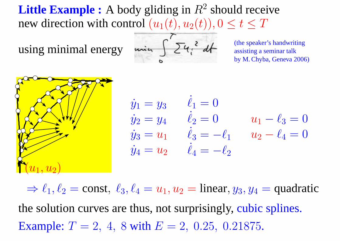
Little Example : A body gliding inR2 should receivenew direction with control(u1(t), u2(t)), 0 ≤ t ≤ T
using minimal energy(the speaker’s handwritingassisting a seminar talkby M. Chyba, Geneva 2006)
(u1, u2)
y1 = y3
y2 = y4
y3 = u1
y4 = u2
ℓ1 = 0
ℓ2 = 0
ℓ3 = −ℓ1
ℓ4 = −ℓ2
u1 − ℓ3 = 0
u2 − ℓ4 = 0
⇒ ℓ1, ℓ2 = const, ℓ3, ℓ4 = u1, u2 = linear, y3, y4 = quadratic
the solution curves are thus, not surprisingly,cubic splines.
Example:T = 2, 4, 8 with E = 2, 0.25, 0.21875.– p.42/45
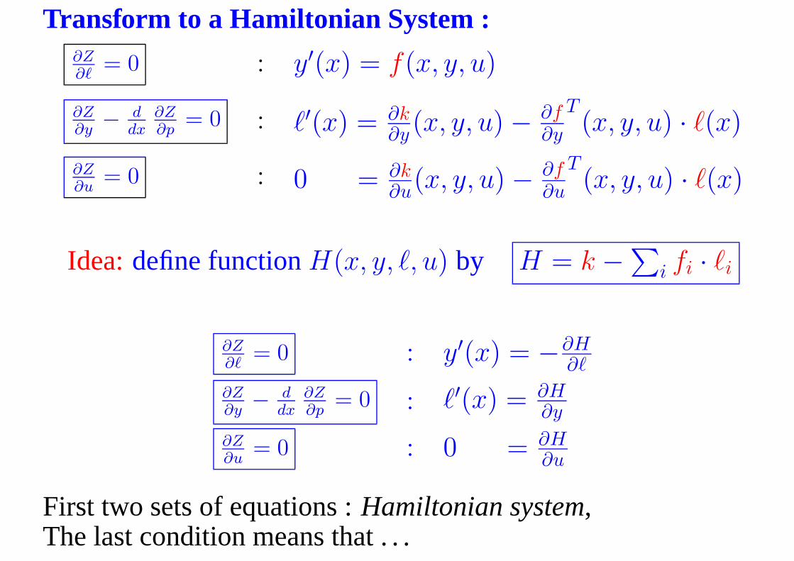
Transform to a Hamiltonian System :∂Z∂ℓ
= 0 : y′(x) = f(x, y, u)
∂Z∂y
− ddx
∂Z∂p
= 0 : ℓ′(x) = ∂k∂y
(x, y, u) − ∂f∂y
T(x, y, u) · ℓ(x)
∂Z∂u
= 0 : 0 = ∂k∂u
(x, y, u) − ∂f∂u
T(x, y, u) · ℓ(x)
Idea:define functionH(x, y, ℓ, u) by H = k −∑
i fi · ℓi
∂Z∂ℓ
= 0 : y′(x) = −∂H∂ℓ
∂Z∂y
− ddx
∂Z∂p
= 0 : ℓ′(x) = ∂H∂y
∂Z∂u
= 0 : 0 = ∂H∂u
First two sets of equations :Hamiltonian system,The last condition means that . . . – p.43/45
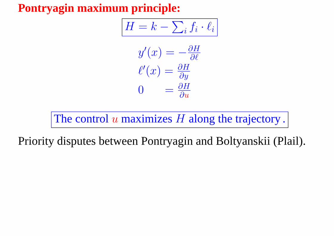
Pontryagin maximum principle:
H = k −∑
i fi · ℓi
y′(x) = −∂H∂ℓ
ℓ′(x) = ∂H∂y
0 = ∂H∂u
The controlu maximizesH along the trajectory .
Priority disputes between Pontryagin and Boltyanskii (Plail).
– p.44/45
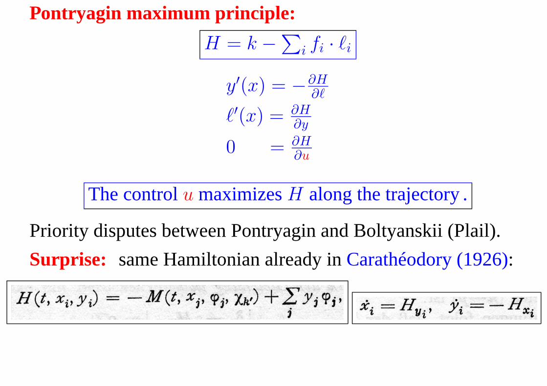
Pontryagin maximum principle:
H = k −∑
i fi · ℓi
y′(x) = −∂H∂ℓ
ℓ′(x) = ∂H∂y
0 = ∂H∂u
The controlu maximizesH along the trajectory .
Priority disputes between Pontryagin and Boltyanskii (Plail).
Surprise: same Hamiltonian already inCarathéodory (1926):
– p.44/45
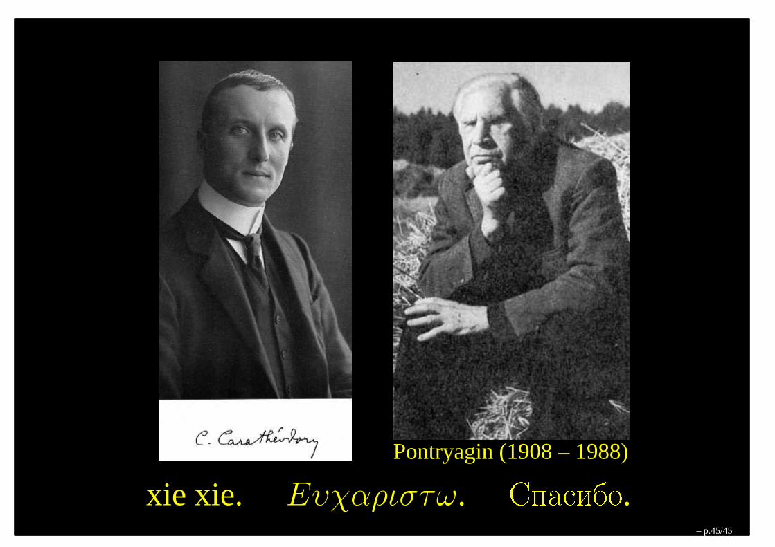
Pontryagin (1908 – 1988)
xie xie. Eυχαριστω. Spasibo.– p.45/45


![[Blair]_Convex Optimization and Lagrange Multipliers (1977)](https://img.pdfslide.net/doc/110x75/577cc4d81a28aba7119aa5b1/blairconvex-optimization-and-lagrange-multipliers-1977.jpg)

