Embed Size (px)
Citation preview
Carlo Borghi
Discrete choice models for marketingNew methodologies for optional features and bundles
Master thesis, defended on November 12, 2009
Thesis advisor: Richard D. Gill
Mastertrack: Mathematics and Science Based Business
Mathematisch Instituut, Universiteit Leiden
Contents
1 Quantitative techniques for marketing 11.1 Conjoint methodologies . . . . . . . . . . . . . . . . . . . . . . . 2
2 Choice-based Conjoint 42.1 What is CBC conjoint . . . . . . . . . . . . . . . . . . . . . . . . 4
2.1.1 Phases of a CBC conjoint study . . . . . . . . . . . . . . 52.1.2 Different estimation procedures . . . . . . . . . . . . . . 72.1.3 A Study example . . . . . . . . . . . . . . . . . . . . . . . 82.1.4 Scenario simulation methods . . . . . . . . . . . . . . . . 112.1.5 Limitations of CBC . . . . . . . . . . . . . . . . . . . . . 12
2.2 Discrete choice models . . . . . . . . . . . . . . . . . . . . . . . . 152.2.1 Derivation of choice probabilities . . . . . . . . . . . . . . 152.2.2 Utilities and additive constants . . . . . . . . . . . . . . . 162.2.3 Utility scale . . . . . . . . . . . . . . . . . . . . . . . . . . 17
2.3 Logit Model . . . . . . . . . . . . . . . . . . . . . . . . . . . . . . 172.3.1 Choice probabilities . . . . . . . . . . . . . . . . . . . . . 172.3.2 Estimation procedure . . . . . . . . . . . . . . . . . . . . 202.3.3 Choice among a subset of alternatives . . . . . . . . . . . 23
3 The Hierarchical Logit model 253.1 Introduction . . . . . . . . . . . . . . . . . . . . . . . . . . . . . . 253.2 Hierarchical models for marketing . . . . . . . . . . . . . . . . . . 253.3 Inference for hierarchical models . . . . . . . . . . . . . . . . . . 283.4 The Hierarchical Bayes multinomial logit model . . . . . . . . . . 28
3.4.1 Estimation for the Hierarchical logit model . . . . . . . . 31
4 Optional features 344.1 Business perspective . . . . . . . . . . . . . . . . . . . . . . . . . 344.2 Summary of business questions . . . . . . . . . . . . . . . . . . . 374.3 Scope of our analysis . . . . . . . . . . . . . . . . . . . . . . . . . 374.4 Methodology . . . . . . . . . . . . . . . . . . . . . . . . . . . . . 384.5 Questionnaire structure . . . . . . . . . . . . . . . . . . . . . . . 38
4.5.1 Intended result . . . . . . . . . . . . . . . . . . . . . . . . 394.6 Assumptions . . . . . . . . . . . . . . . . . . . . . . . . . . . . . 39
4.7 Simulations . . . . . . . . . . . . . . . . . . . . . . . . . . . . . . 404.7.1 Answer generation procedures . . . . . . . . . . . . . . . . 414.7.2 Set of utilities . . . . . . . . . . . . . . . . . . . . . . . . . 41
4.8 Estimation procedures . . . . . . . . . . . . . . . . . . . . . . . . 424.9 Measures of fit . . . . . . . . . . . . . . . . . . . . . . . . . . . . 454.10 Simulation results . . . . . . . . . . . . . . . . . . . . . . . . . . 454.11 Overview of results . . . . . . . . . . . . . . . . . . . . . . . . . . 484.12 Conclusions . . . . . . . . . . . . . . . . . . . . . . . . . . . . . . 51
5 Optional features study 525.1 Study description . . . . . . . . . . . . . . . . . . . . . . . . . . . 52
5.1.1 Description of the attributes and levels . . . . . . . . . . . 535.2 Business questions . . . . . . . . . . . . . . . . . . . . . . . . . . 545.3 Old estimation procedure . . . . . . . . . . . . . . . . . . . . . . 545.4 The new methodology . . . . . . . . . . . . . . . . . . . . . . . . 555.5 Simulation procedures . . . . . . . . . . . . . . . . . . . . . . . . 56
5.5.1 Improvement over old estimation procedure . . . . . . . . 57
6 Bundles 596.1 the Bundle study . . . . . . . . . . . . . . . . . . . . . . . . . . . 606.2 Differences and similarities with optional features . . . . . . . . . 60
6.2.1 Interaction effect . . . . . . . . . . . . . . . . . . . . . . . 616.2.2 Goals of the model . . . . . . . . . . . . . . . . . . . . . . 616.2.3 Limitations of the model . . . . . . . . . . . . . . . . . . . 61
6.3 Utility from a business perspective . . . . . . . . . . . . . . . . . 62
7 Results of the Bundles study 637.0.1 Characteristics of the study . . . . . . . . . . . . . . . . . 637.0.2 Choice task design . . . . . . . . . . . . . . . . . . . . . . 677.0.3 Attributes . . . . . . . . . . . . . . . . . . . . . . . . . . . 687.0.4 The choice tasks . . . . . . . . . . . . . . . . . . . . . . . 707.0.5 Results . . . . . . . . . . . . . . . . . . . . . . . . . . . . 747.0.6 Comment on the coding . . . . . . . . . . . . . . . . . . . 75
8 CBC HB estimation algorithm in R 838.1 Running the program . . . . . . . . . . . . . . . . . . . . . . . . 83
8.1.1 Design matrix and answers . . . . . . . . . . . . . . . . . 848.1.2 Prior parameters . . . . . . . . . . . . . . . . . . . . . . . 858.1.3 Running the algorithm . . . . . . . . . . . . . . . . . . . . 85
8.2 Output files . . . . . . . . . . . . . . . . . . . . . . . . . . . . . . 86
Abstract
The topic of this Master Thesis is quantitative methodologies for optionalfeatures and bundles. The frame is the one of Quantitative Marketing Research,a field whose goal is to give market intelligence in forms of, among others, marketshares, population clustering and scenario simulations. The particular problemwe have worked on is the one of optional features and bundles i.e. services thatcan be selected for an extra price when purchasing a product.The technique we have used in our analysis is a discrete choice model, Choice-based Conjoint.
The content of this thesis is based on an internship at the internationalmarket research company SKIM. The internship was jointly supervised by Se-nior Methodologist Kees van der Wagt (SKIM) and Prof. Dr. Richard Gill(Mathematisch Instituut Leiden).
The two most important results of the thesis are new methodologies to studyproducts with optional features and bundles. These methodologies produce util-ities that match the respondent’s observed choices. Only knowing the estimatedutilities, we are able to answer the questionnaire producing answers similar tothe observed ones.The methodologies enjoy all typical properties of conjoint methodologies andcan be used to calculate market shares, simulate scenarios etc.Their most interesting feature is that it is possible to tell if offering an optionmakes a product too complicated. They can also tell if their simple presencemakes the product more appealing (halo effect).
As far as we know, this is the first study in this promising field.The methodologies we propose are tested on two different datasets arising fromstudies conducted by SKIM. They have been developed with tests on simulateddatasets.The software of choice for the estimation procedure was Sawtooth’s implemen-tation of CBC HB. For reproducibility of experiments we also wrote a packagein the open source language R reproducing the same algorithm. This packageand Matlab codes used in simulations are found in the Appendix.

Chapter 1
Quantitative techniques formarketing
Market research is the discipline of analyzing and exploring markets. The goalis to acquire valuable information that can be used in taking strategic marketingdecisions.The scope of market research is extremely wide and, depending on the kind ofdecision to be taken extremely different techniques can be used.
For example, a firm in the automotive industry may be interested in fore-casting the state of the market in the following years. They may be interested inknowing how consumers respond to their advertisement. Are the cars they pro-duce a status symbol? What kind of feeling do they elicit in customers? Whatkind of people their customers are, in terms of age, income, sex? And who arethem, in terms of aspirations, values, and dreams? They could be interested in aprecise financial forecast of the sale of a new model. How people would respondto a completely different kind of cars being launched on the market? What kindof options should they offer with their cars? Is their offering of cars balanced?What is the optimal price for their line of products? All these questions fallwithin the scope of market research. They are extremely different, and needcompletely different methodologies to be answered.
At the most general levels, market research can be divided in two kinds:qualitative and quantitative. Qualitative market research is focused on under-standing customers by considering them singularly. The goal is to understandwhat drives people in their choices or what their perception is of a certain brandor product. Often qualitative research involves panels and in depth discussionabout perceived characteristics of a product with a restricted number of studysubjects. The goal of qualitative techniques is to give a deep market under-standing. In this sense, qualitative methodologies are useful to shape a strategybut are not per se a tool to take decisions.
Quantitative techniques usually provide market understanding based onsound data. The goal is to provide financial forecasts, market shares calcu-
CHAPTER 1. QUANTITATIVE TECHNIQUES FOR MARKETING 2
lations, scenario analysis, clusterings of populations. These methodologies areespecially good for taking strategic decisions. Usually quantitative techniquesrely strongly on statistical techniques to give robust results.
1.1 Conjoint methodologies
Conjoint methodologies are a particular kind of methodologies for quantitativemarket research. They are based on direct data collection: data are collectedespecially for each study and no historical data is used.Further more, they are based on experiments: research participants have tocomplete carefully engineered exercises that will show their buying behavior.
The roots of conjoint methodologies lie in experimental psychology and psy-chometrics. This techniques have been used in marketing since 1980s.
In the conjoint experiments respondents have to consider a finite set of prod-ucts and state their preference(s) in form of choices, numerical ratings or order-ing best-to-worst.
The products shown are usually described by a list of their features andsometimes by a picture. Those can be features already present on the marketor new features that will be introduced in the future. The ability to studyreactions to new features is a strong point for conjoint methodology. It makespossible to study scenarios in which completely new products are introduced.No methodology based on historical data can do such a thing.
The name conjoint is derived from the fact that data is obtained by showingrespondents a situation in which they have to evaluate a product in its integrity.Therefore, their preferences for single elements of that product are consideredjointly.In other methodologies respondent may be asked to consider attributes one byone and evaluate them. For example they could be asked to indicate how impor-tant for them is to have a GPS included in the price, or what is the maximumprice they would consider paying for a given model of car. In conjoint method-ologies, respondents only state preferences about full products. Therefore, theirpreferences (for attributes) are considered jointly. From these joint preferencesit is possible to work out the preferences for single attributes and the trade-offbetween different attributes.
Conjoint methods are at the moment the standard of the market and theyhave huge advantages over other methods present on the market. First of all,in market research data availability is one of the most critical issues.
Collecting the right data is always difficult and decisions based on a biasedor senseless dataset can be disastrous. Many techniques make predictions bylooking at historical data and past trends and then extrapolating the resultsinto the future. These techniques can capture trends but are of no use when acompletely new product enters the market. Also, it is very hard or sometimesimpossible to access sales time series for competitor’s single products.
CHAPTER 1. QUANTITATIVE TECHNIQUES FOR MARKETING 3
Other techniques are based on data collected at market points (supermar-kets, shops etc.). It is very hard to tell if this data is really representative ofthe whole sample, and it is almost impossible to tell what will happen in case anew product is launched on the market.
The strength of conjoint analysis with respect to such techniques is that it isbased on primary data collection. Data is gathered for the specific need of thestudy. For this reason, the researcher can control the way the random sampleis generated and can ask questions of interest.
Another great advantage of conjoint techniques is realism. Conjoint choicetasks usually involve the choice between a number of products that are shownin their integrity. This is very similar to an actual choice purchase and thereforeit is a not very demanding task. Also, realism in the choice task gives realisticanswers. Ratings given when considering a single feature can be extremelymisleading. It is a well known fact that such self-explicated preferences can bevery unrealistic. Most people are not able to work out the importance theygive to a single attribute. Generally, people tend to state many features aremust-have: so important that they will not consider products without them. Inreality, most of them are willing to make a trade-off.
Conjoint exercises are mostly of three kinds. Traditionally it was adminis-tered as a ranking exercise, when the respondent has to rate some products frommost interesting to least interesting. It could also be a rating exercise (wherethe respondent awards each trade-off scenario a score indicating appeal).
In more recent years it has become common practice to present the trade-offs as a choice exercise. The respondent simply chooses the most preferredalternative from a selection of competing alternatives. This is the most realistictype of exercise, since it mimics actual behavior in the market. In case of achoice exercise, we speak of Choice-Based Conjoint or CBC.
A special kind of choice exercises are constant sum allocation exercises. Re-spondents are asked to allocate a fixed number of purchases among a set ofproducts. This is meant to represent a series of purchases. The respondent isfree to select (i.e. buy) a single product as many times as he/she wants. Thiskind of exercise is appropriate for products for which consumers show a varietysearching behavior. It is also particularly common in pharmaceutical marketresearch, where physicians are given a patient description and have to specifyhow often are they going to prescribe each of the alternatives. In this case eachalternative is the description a real or hypothetical drug/therapy.For the point of view of estimation, each allocation is considered as independentfrom the other. Therefore, an allocation exercise with a total sum of 5 is con-sidered as 5 independent CBC questions. This mean that the same estimationprocedure for CBC can be used.
Conjoint estimation is traditionally carried out with some form of multipleregression model, but more recently the use of hierarchical Bayesian analysishas become widespread, enabling the study of data at a respondent’s level.
Chapter 2
Choice-based Conjoint
2.1 What is CBC conjoint
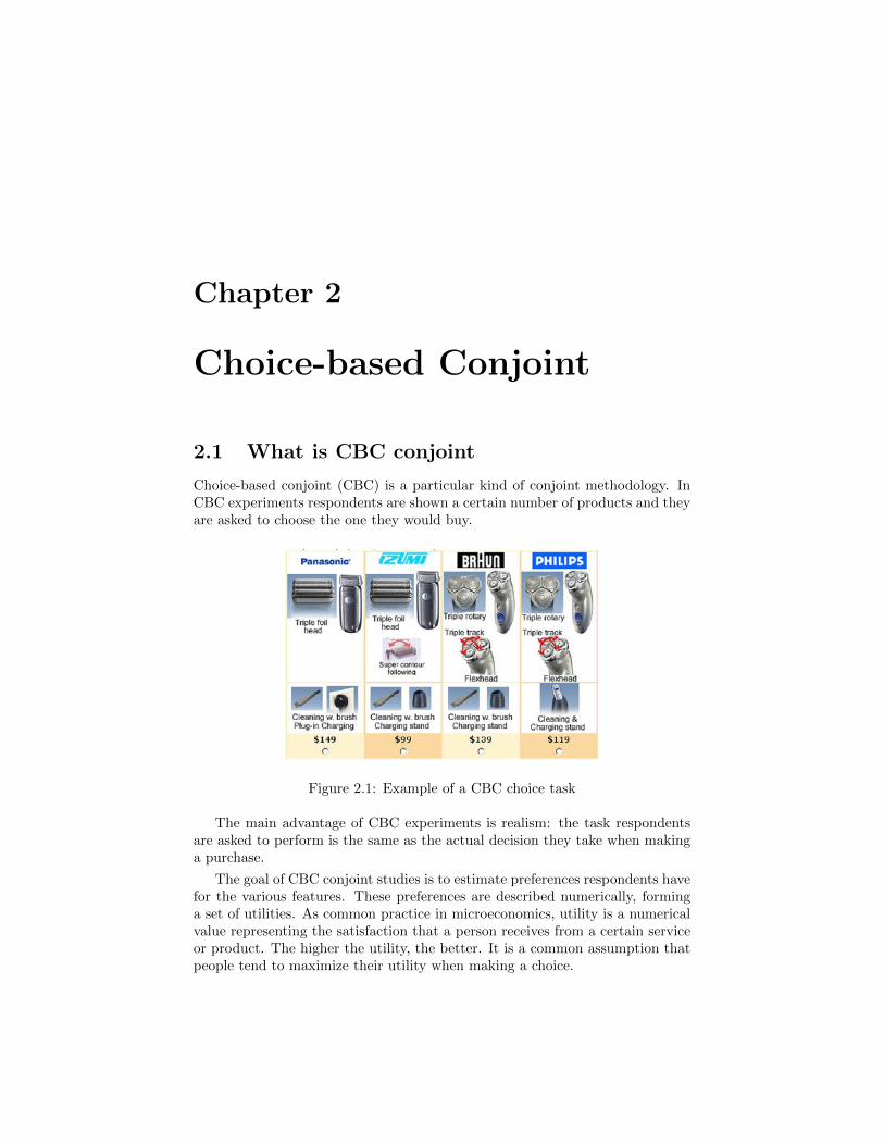
Choice-based conjoint (CBC) is a particular kind of conjoint methodology. InCBC experiments respondents are shown a certain number of products and theyare asked to choose the one they would buy.
Figure 2.1: Example of a CBC choice task
The main advantage of CBC experiments is realism: the task respondentsare asked to perform is the same as the actual decision they take when makinga purchase.
The goal of CBC conjoint studies is to estimate preferences respondents havefor the various features. These preferences are described numerically, forminga set of utilities. As common practice in microeconomics, utility is a numericalvalue representing the satisfaction that a person receives from a certain serviceor product. The higher the utility, the better. It is a common assumption thatpeople tend to maximize their utility when making a choice.
CHAPTER 2. CHOICE-BASED CONJOINT 5
From a mathematical point of view, CBC is part of the family of discretechoice models. Those are econometrics models describing a choice among adiscrete, finite set in terms of utility. We’ll describe those models from a formalpoint of view, specifying their structure in mathematical terms and illustratingthe estimation procedure, in section 2.2.
First we will explain the phases of a conjoint study and the assumption andlimitations of CBC models.
2.1.1 Phases of a CBC conjoint study
These are five phases in a typical CBC conjoint study:
1. Problem definition and questionnaire generation
2. Screening
3. Data collection
4. Estimation
5. Follow-up
1. Problem definition and questionnaire generation
The first phase of a conjoint study is to define the characteristics of the marketthat is to be studied and the business questions that one wants to answer.
The first and most important phase is to decide what attributes should beincluded in the product description.It is important to choose which attributes are considered in the study: if thedescription of a product has too many attributes, respondents will not considerall of them but will place importance to only a few. This is known as a sim-plification strategy. The use of such strategies by the respondent can greatlyimpair the estimation procedure: conjoint methodologies are based on the factthat all attributes have a weight in making decisions.
The number of question is also important: choosing too many questions perrespondent will make the questionnaire more tiring to answer and respondentswill start to give senseless answers. Experienced market researcher advise tolimit the number of CBC chioce tasks under 14.
After the problem is defined, a different questionnaire is generated for eachrespondent.The goal of having different questionnaires is to show all possible levels combi-nations.
2. Screening
Often a screening is performed on the respondents. Different screening proce-dures can be applied: one procedure can be the screening performed ex ante,
CHAPTER 2. CHOICE-BASED CONJOINT 6
before the respondent will answer any of the questions of the survey. Anotherprocedure is the screening performed during the questionnaire answering. Usu-ally CBC studies have many demographic questions before the actual CBCexercise starts.
In general the first type of screening happens when the study is set up andthe questionnaire is sent to respondents.This type of screening is easier to control by the person who set up the ex-periment, because sending the questionnaire to a certain sample with specificcharacteristics depends only on the decision of the study maker. The goal ofex-ante screening is to obtain a representative sample or a population with cer-tain characteristics.For example: in evaluating a new tofu based product, we may want half of thepopulation to be vegetarians and half non-vegetarians, because we know thatfor this class of products the market is segmented in such a way.
The second type of screening in general happens during the first part of thequestionnaire, and is often based on demographic information. This type ofscreening can be less controlled by the study maker, since it depends totallyon the way respondents answer to the questions and therefore it is potentiallymore subject to bias. For example, for a product for teenagers, we may want toscreen out respondents that declare their age to be over a certain threshold.
However, it must be take into account that, if the group of people beingstudied has any form of control over whether to participate in the study, the socalled self-selection bias may arise. Indeed participants’ decision to participatemight be correlated with traits that affect the study making the participants anon representative sample. Self-selection bias is hard to track down and can bethe cause of very biased results.
3. Data collection
Respondents answer the questionnaire. The questionnaire can be an actualpaper module to be compiled. Today, more and more questionnaires are com-pleted on the internet. Internet questionnaires are cheaper, more time-effectiveand they are getting increasingly popular.However, internet surveys are known for generating less precise answers andthe number of fraudulent respondents (respondents answering casually) is muchhigher than with paper and pencil surveys.Usually data such as the time spent to compile the questionnaire is used toscreen out too fast respondents.
4. Estimation
Based on the collected data, utilities are estimated.
Using different algorithms, it is possible to estimate utilities for the wholepopulation considered as one, for homogenous groups of respondents and alsofor each respondent.We will explain in detail the estimation procedure in the next sections.

CHAPTER 2. CHOICE-BASED CONJOINT 7
5. Follow up
The estimated utilities are used to develop market insight.Given the utilities, it is possible to calculate market shares for different products.It is possible to set the current market situation as the base scenario and seehow shares change when a change is introduced in the market.For some populations clearly defined segments may be present, and it is possibleto track them down, dividing the population in homogenous groups with similartastes.It is possible to study interaction between certain attributes. We can calculateprice sensitivity curves at an aggregate, group or respondent level. We can seehow the value of a brand is perceived among respondents, and what featureshave more weight in the choice decision.
2.1.2 Different estimation procedures
As we mentioned earlier, there are different ways to analyze the data collectedin a conjoint study. The most important methods are Aggregate Logit, LatentClass and CBC HB. They respectively provide utilities for the whole respondentspopulation, for homogeneous groups in the population and for each componentof the population.
Aggregate logit
In this model the whole population of respondents is considered in its integrity.The result is a single set of utilities for the whole population. Intuitively, theresulting utilities describe an average of the population preferences.
Aggregate estimation assumes that the respondent utility is equal to theaverage utility, which is a quite restrictive assumption and does not allow foridiosyncratic, individual effects in the sample, meaning that heterogeneity inthe sample is simply not considered. This was the first model ever implementedto analyze conjoint data. We will explain in detail this model in section 2.2.1.
Latent Class
Cluster analysis is, historically speaking, the evolution of aggregate estimation.It was developed to allow for some form of respondents heterogeneity.
Clustering algorithms find groups of individuals with similar tastes amongthe whole sample. The preferences of the individuals are estimated in a ”semiindividual” way by assuming that the respondent utility is equal to the clus-ter utility, allowing for heterogeneities across segments of respondents but notwithin the cluster. To allow for heterogeneity between single respondents, HBmodels were created.
Clustering models are still very important in their own respect. From acommercial point of view it is very important to divide the market in segmentsthat have similar tastes.

CHAPTER 2. CHOICE-BASED CONJOINT 8
Latent Class estimation detects subgroups of respondents with similar pref-erences and estimates utilities for each segment. Each respondent is given aprobability to being part of a certain group.It is possible to specify how many groups are to be considered. There are cri-teria (notably the Akaike criterion) to decide the optimal number of groups toconsider.
CBC HB
HB methods are the newest and currently most used estimation methods inquantitative marketing research.The name CBC HB means ”Choice Based Conjoint - Hierarchical Bayes”. Themathematical specification of these model is a Bayesian hierarchical model inwhich, broadly speaking, a different vector of utility is define for each respon-dent. The distribution of these utilities in the whole population has some spec-ified form, usually normal.
CBC HB allows for heterogeneity at a respondent’s level by specifying dif-ferent utilities for each respondent. This leads to a greater improvement in sim-ulation techniques: simulation conducted using aggregate or clusterized modelsoften lead to biased results.We will devote most of chapter 3 to explain the details of this model.
2.1.3 A Study example
To make things clearer, we show what the result of a CBC study would looklike.Suppose we are interested in the market of smartphones.We think the most important features are of course price, then brand, screensize, internal memory, operative system and if there is a keyboard or a touchscreen. These are by no mean all attributes, but we must limit the number ofattribute to study to have meaningful answers from the respondents.
Considering some phones on the market, we decide to these attributes cantake the following values:
• Price: 220 euro, 230 euro, .....490 euro, 500 euro
• Brand: Nokia, Samsung, Blackberry, LG
• Screen size: 2.8”, 3”, 3.2”, 3.5”
• Internal memory: 2 Gb, 4 Gb, 8 Gb, 16 Gb
• Full keyboard: present/not present
• Touch screen: present/not present
For example a Nokia E63, a model really present on the market, is defined bythe following vector of attribute levels: (240 euro, Nokia, 3”, 4 GB, present, notpresent).

CHAPTER 2. CHOICE-BASED CONJOINT 9
A choice task with 4 alternatives is a list of 4 configuration vectors. Thesedon’t need to represent any phone really present on the market and ca be com-pletely casual. A typical choice task would look something like
Choose one of the following
Product 1 Product 2 Product 3 Product 4Price 300 250 230 370Brand Nokia Blackberry Samsung LGScreen size 2.8” 3.2” 3.2” 3”Internal Memory 2Gb 4Gb 8Gb 8GbFull Keyboard present not present present not presentTouch screen not present present present present
After collecting the answers to the choice tasks, we can perform the estima-tion.If using a the aggregate logit model, we will obtain a single vectory of utilities.We have an utility for each level. For each attribute will we obtain the utilities:
Brand:Nokia Brand:Samsung Brand:LG Brand:BlackberryUtility 2.18 0.4 3.24 -0.76
Screen size: 2.8 Screen size: 3 Screen size: 3.2 Screen size: 3.5Utility 4.30 -0.74 -1.64 2.96
and so on.
In case we used CBC-HB, we would have different utilities for each respon-dent:
Brand:Nokia Brand:Samsung Brand:LG Brand:BlackberryResp. 1 2.18 0.4 3.24 -0.76Resp. 2 4.23 -0.82 1.96 2.28. . . . . . . . . . . . . . .Resp. 300 2.193 1.12 2.93 -1.20
Suppose we are interested in the market shares in a given scenario. Forscenario we intend the situation of available products on the market.
First we define the products available on the market. Just for the example’ssake, we consider a market with only 4 products.
Market situation

CHAPTER 2. CHOICE-BASED CONJOINT 10
Product 1 Product 2 Product 3 Product 4Price 300 250 230 370Brand Nokia Blackberry Samsung LGScreen size 2.8” 3.2” 3.2” 3”Internal Memory 2Gb 4Gb 8Gb 8GbFull Keyboard present not present present not presentTouch screen not present present present present
To calculate the market share of each phone, we first calculate each phone’sutility. The utility of the phone is just the sum of its features utilities.
Let’s first consider the case of Aggregate Logit. This is what we may find:
Product 1 Product 2 Product 3 Product 4Utility 10,23 11,67 4.48 9,24Exp(Utility) 27722 117008 73130 10301
Market share 12,5% 51% 32% 4,5%
To calculate market shares, we use a method known as share of preference.In this method, we first exponentiate each product utility. The market shareof one product is that product exponentiated utility divided by the sum of allproducts exponentiated utilities.This way, the market share of each product is proportional to its exponentiatedutility.
If we used the CBC HB algorithm, we can calculate product utilities for eachrespondent.
Utility per respondent Product 1 Product 2 Product 3 Product 4Resp 1 10,23 11,67 4.48 9,24. . . . . . . . . . . . . . .Resp 300 16,76 12,67 14.78 12,5
In this case to calculate market shares we can use again share of preference,calculating a vector of market shares for each respondent. The final market shareof a product is the average of the market shares calculated for each respondent.However, it’s also possible to calculate shares in a different way. We imagineeach respondent is making a single choice, and we assume he/she would chosethe product with the highest utility.So for example Respondent 1 would choose product 2 and respondent 300 wouldchoose product 1.At the end the market share of a product is the number of times it was chosendivided by the number of respondents. This method of calculating market sharesis called First Choice.
We are now going to explain the reasons behind the use of these two methods.

CHAPTER 2. CHOICE-BASED CONJOINT 11
2.1.4 Scenario simulation methods
The ability to perform scenario simulations is the most interesting feature ofconjoint studies.Using the estimated utilities,we can calculate market shares of the productspresent now on the market. We can see what happens when an existing productchanges its design or price, or when a new product enters the market.Further more, it is possible to see what would happen if a completely new classof products enters the market.
The most interesting simulations are calculated with CBC-HB models, wherewe can simulate the choice of every single respondent.
There are mainly three methods to simulate choice, namely first choice, shareof preference and randomized first choice.First choice assumes that each respondent chooses one product (the one maxi-mizing utility), while share of preference (also called logit simulation) indicatesfor each respondent a share of purchase for each product, proportional to theirutilities.Randomized first choice is somehow an alternative in between the two previousmethods: each respondent chooses a single product with a probability propor-tional to their utilities.
In first choice of preference the product with the highest utility is chosenby the respondent, and then the share of products across respondents is cal-culated by dividing the number of respondents choosing that product by thetotal respondents. This method relies on the assumption that the respondentdoesn’t have a variety seeking behavior and spends enough time considering thepurchase, being able to identity the product with the highest utility.
This method makes sense for purchase decisions that respondents evaluatecarefully and that involves huge amounts of money, such as the purchase of acar or a house.
Share of preference method assumes a probability distribution across prod-ucts for each respondent. For each respondent, the exponential of each product’sutility, divided by a normalizing constant, is the share of preference of that prod-uct for that respondent.This method makes sense for products where several purchases are made in acertain period. For example, when considering products like jam consumer donot always buy the one they like most and they are likely to buy different tastesin different purchases.Since it is based on a distribution of preferences, share of preference provides aflatter distribution of shares with respect to first choice.Share of preference is to be preferred for those product whose purchase is notvery carefully considered or for which there may be a variety seeking behavior.Examples are CPG products like biscuits, chips, soft drinks etc.
CHAPTER 2. CHOICE-BASED CONJOINT 12
2.1.5 Limitations of CBC
The CBC model is such a powerful and easy tool that one can be seduced intousing it to analyze all marketing problems. Indeed, despite (or we could say,because of) its great scope of analysis, the CBC model has to be used with care.
The first limitation is not a limitation of the model itself, but rather of therespondents. Cognitive psychology experiments have confirmed what marketersknew from long time: people can answer a very limited number of choice tasksbefore loosing interest and motivation and answering just randomly.As a rule of thumb, no more than 14 questions should be asked to each respon-dent in a conjoint study. A common way to discriminate well thought answersfrom random clicks is to analyze the amount of time a respondent spends ana-lyzing each question.
The amount of time spent for each choice task diminishes invariably aftereach question. This can be explained both by a progressive lack of motivationand by the fact that respondents get experience in performing choice tasks.There is evidence that well motivated respondents take less time to answerchoice tasks as they get more accustomed to the characteristics of the productsshown.
Another factor to consider is the number of features: each product should bemade of a number of attributes limited enough that the respondent can considerall of them at once. If this is not the case, respondents will apply simplificationstrategies: they will base their choice only on some of the attribute shown,considering the other unimportant. This gives unrealistic results.It is advisable not to use more than 7 features.
In the specification of the model, attributes evaluation of one product shouldbe independent of each other. For example, in a car study the utility for a singlerespondent for the color blue or red should be independent from the brand ofthe car.However, what happens in reality is that for most people the color Red is moreappealing when offered with a Ferrari than with a Porsche. That is, there is aninteraction between two attributes.
For most products an assumption of independent features is not always re-alistic and sometimes is just wrong. It is possible to estimate the interactioneffect between two attributes.
If an interaction effect is known to be present between two attributes, acommon practice is to add the two attributes in one.In the setting of the previous example, we would start with the attributesBrand: Ferrari, Porsche, Jaguar (3 levels) Color: Red, Dark green, Silver (3levels)In this case, the results may show people having a strong preference for silver
CHAPTER 2. CHOICE-BASED CONJOINT 13
or red or dark green. So the model would tell us that a Silver Ferrari would bebetter than a Red Ferrari, something we know is not true.
The solution is to consider a new attribute made of all the combinationsof the previous ones: Brand+color: Red Ferrari, Dark green Ferrari, SilverFerrari, Red Porsche, Dark green Porsche, Silver Porsche, Red Jaguar, Darkgreen Jaguar, Silver Jaguar (9 levels)In this way we would be able to see correctly that the utility for a Red Ferrariwould be much better than the one for a Dark Green Ferrari and so on.
In less extreme cases, it is possible to ignore the interaction. Market sharesare quite consistent even in this case.
It is a well know fact by marketers that people can show much different pricesensitivity in real market than in choice experiments.For example, when buying a bag of chips most people don’t really spend toomuch time considering the price, given it is in an ”acceptable” range and justpick one bag that has a taste they like.When performing a choice task in a conjoint experiment about chips, the sameperson may be taken to consider its purchase in a much more precise way.Therefore he/she may show much higher price sensitivity.There is no real way to see if the results show too much price sensitivity otherthan having some experience with one market. The best way to solve this isto re-scale the price utilities by some constant and then doing simulations asalways.
When studying a market scenario, one may be interested in comparing thepredicted shares of the current scenario to the ones measured on the market. Indoing so, one could be quite disappointed as the estimated market shares maybe quite far from the actual ones.
This is not a reason for concern: the results from a conjoint study may beperfectly reasonable and very worthy even when they are not able to predictthe current market share.This is because the conjoint market shares are calculated in a much idealizedcondition: all customers have perfect information about the products, all theproducts are accessible to all consumers and the customers are driven in theirchoice only by the features of the product rather than promotions, advertisementcampaigns and so on.So for example, from a CBC study on cigarettes we expect the resulting marketshares to be extremely precise since there are few products on the market andthey are pretty much available everywhere.
For other products like cars it may be more complicated: respondents mayshow great interest in a particular Hyundai model, giving a simulated marketshare much higher than the real one. This may be due to the lack of Hyundaisellers in the country, or to some aggressive price promotion by competitors, orto public founding for certain type of cars.This doesn’t mean that the conjoint results are not useful.
When a firm has to take a strategic decision it must compare the market

CHAPTER 2. CHOICE-BASED CONJOINT 14
share in the current (simulated) scenario and the one in a new scenario. Theonly thing that matters is the difference between the two.Since conjoint studies deliver ideal shares, they filter all external influences onmarket share.
In this sense, ideal market shares are even better to understand modificationsin the market scenario. This is even better when taking a strategic decision.If the aim is to get a precise financial forecast, it is possible to correct idealmarket share to take into account external factors.
When considering the scenario results of a conjoint study (for example amarket share for a certain product) it must also be noted that those are peakresults.For example, even for a perfect representation of people’s tastes and in a marketscenario that will not change in the immediate future, the market share of a newproduct will not be achieved right away after its launch.
It takes time for people to switch from one product to the new one andtypically you have to educate people about the features of the new product andsome people just take a lot of time to decide to switch.To estimate the amount of time needed to reach this peak share a generalknowledge of the market is needed. In some markets it takes a great deal oftime to convince people to switch from the product they are using, while inothers it is way easier.
Variety searching is a well documented behavior, both in marketing practiceand econometric theory. When making a choice, customers do not always choosetheir ideal but like to try other products. This is especially true for consumerpackaged goods (CPG), inexpensive products that are purchased regularly likefood, drinks etc.
The opposite of variety searching is habit forming: the tendency of customersto stick to the product they are already buying even when a new product, closerto their ideal, enters the market.
Furthermore, certain products may have some sort of barrier to change. Auser of a certain product may encounter trouble when wanting to switch toanother one because of the existence of a contract, or because of costs to betaken when switching.Think for example of an office that wanted to switch from Microsoft Windowsto an Apple OS: most of their software licenses would be useless and they wouldhave to change most of the hardware.
CBC market shares don’t account for all this issues: if a new product isfeatured in a scenario, its market share will not consider barriers to change andprevious habits of customers.To conclude, CBC shares are much idealized: they are calculated as if customers
CHAPTER 2. CHOICE-BASED CONJOINT 15
had perfect knowledge of all the alternatives and had no history, as if they werein the market for the first time and not locked to any brand or product.
2.2 Discrete choice models
Discrete choice models are models used in econometrics to describe choices byrational actors in a finite set.These models describe the choice as depending from some observable character-istics of the elements in the set and some parameters, unknown to the researcher,called utilities.The model used for conjoint studies is also called logit model and is special casesof discrete choice models.
2.2.1 Derivation of choice probabilities
Utility represents the benefit gained when selecting an element of the set.Discrete choice models are usually derived under an assumption of utility-maximizing behavior by the decision maker.
A decision maker, labeled n, faces a choice among J alternatives. We assumethe respondent would obtain a certain level of utility from each alternative. Theutility that decision maker n obtains from alternative j is Unj , j = 1 . . . J .
This utility is known to the decision maker but not by the researcher. Thedecision maker chooses the alternative that provides the greatest utility. Thebehavioral model is therefore: choose alternative i if and only if Uni > Unj∀j 6=i.
From the researcher’s point of view, it is not possible to observe the decisionmaker’s utility. The only thing that can be observed is some attributes of the al-ternatives, which we will call xj . It is also possible to define some attribute of thedecision maker, called βn and to specify a function that related these attributesto the decision maker utility. This function is denoted Vnj = V (xnj, βn)∀j andit is usually called representative utility.
Utility is decomposed as Unj = Vnj + εnj, where εnj captures the factors thataffect utility but are not included in Vnj . This decomposition is fully general,since εnj is defined as simply the difference between true utility Unj and the partof utility that the researcher captures in Vnj.
Given this definition, the characteristics of εnj, such as its distribution, de-pend critically on the researcher’s specification of Vnj.
Usually the researcher specifies the analytical form of Vnj and εnj according toa model describing his/her assumptions about the choice. The xnj’s are usuallyconsidered known (as they describe the choice alternatives) and the interest ofthe researcher is to find values of the parameters βn that in some sense betterdescribe the observed choices.
The researcher does not know εnj∀j and therefore treats these terms as ran-dom. They are usually called error terms. The joint density of the random
CHAPTER 2. CHOICE-BASED CONJOINT 16
vector εn = (εn1, . . . εnj) is denoted f(εn).Knowing the density, the researchercan make probabilistic statements about the decision maker’s choice. The prob-ability that decision maker n chooses alternative i is
Pni = P (Uni > Unj,∀j 6= i)= P (Vni + εni > Vnj + εnj,∀j 6= i)= P (εnj − εni < Vni − Vnj,∀j 6= i)
(2.1)
This probability is a cumulative distribution, namely, the probability thateach random term εnj − εni is below the observed quantity Vni − Vnj.
Using the density f(εn) the cumulative probability can be rewritten as
Pni = P (εnj − εni < Vni − Vnj,∀j 6= i)
=
∫ε
I(εnj − εni < Vni − Vnj,∀j 6= i)f(εn)dεn
where I(.) is the indicator function, equaling 1 when the expression in parenthe-sis is true and 0 otherwise. This is a multidimensional integral over the densityof the unobserved portion of utility, f(εn). Different discrete choice modelsare obtained from different specifications of this density, that is, from differentassumptions about the distribution of the unobserved portion of utility. Theintegral takes a closed form only for certain specifications of f(.). Logit modelshave closed form expressions for this integral.
2.2.2 Utilities and additive constants
If a constant is added to the utility of all the alternatives, the alternative withthe highest utility doesn’t change. Since the respondent always chooses thealternative with the highest utility, the choice is the same with Unj∀j as withUnj + k∀j for any constant k. Therefore from the respondent’s point of view,the absolute value of the utility is meaningless and the only thing that countsis the difference with the other utilities.
Things don’t change from the researcher’s perspective. The choice probabil-ity is Pni = P (Uni > Unj,∀j 6= i) = P (Uni − Unj > 0,∀j 6= i), which dependsonly on the difference in utility, not its absolute level.
When utility is decomposed into the observed and unobserved parts, equa-tion 2.1 expresses the choice probability as Pni = P (εnj−εni < Vni−Vnj,∀j 6= i)which also depends only on differences between utilities.
Therefore, since utilities are defined up to an additive constant, the absolutevalue of utility can not be estimated, as there are different sets of utilities leadingto the same choices. This must be taken into consideration when comparing twosets of utilities.
CHAPTER 2. CHOICE-BASED CONJOINT 17
2.2.3 Utility scale
We have seen that adding a constant to all utilities doesn’t change respondent’sbehavior as the alternative with the highest utility doesn’t change. The samehappens when multiplying all utilities for a given positive constant.
The model U0nj = Vnj + εnj is equivalent to U1
nj = λVnj + λεnj for any λ > 0:the alternative with the highest utility is the same no matter how utility isscaled. To take account of this fact, we have to normalize the scale of utility.
We can normalize the scale of utility by normalizing the variance of the errorterm. When utility is multiplied by λ, the variance of each εnj is multiplied byλ2: var(λεnj) = λ2 var(εnj).
When error terms are assumed to be i.i.d. (as it is for most models) it iseasy to normalize the error variance of all terms setting it to some value usuallychosen for convenience.
The error variances in a standard logit model are usually normalized to π2
6 .
In this case, the model becomes Unj = x′nj(β/σ) + εnj/σ with var(εnj) = π2
6 σ.
2.3 Logit Model
2.3.1 Choice probabilities
Let’s consider again the general discrete choice model in which decision makern chooses among J alternatives.
The utility of a given alternative j is decomposed into a part labeled Vnj thatis known by the researcher up to some parameters and an unknown part εnj (theerror term) that is treated by the researcher as random: Unj = Vnj + εnj∀j. Thelogit model is obtained by assuming that each εnj is independently identicallydistributed Gumbel with location parameter µ = 0.
The density for each unobserved component of utility is
f(εnj) =e−εnj
σe−εnj−µ
σ
and the cumulative distribution is
F (εnj) = exp(− exp(−εnj − µσ
)) (2.2)
The variance of this distribution is π2
6 σ.
To normalize the scale of utility the variance of the εnj terms is set to the
standard values π2
6 by dividing Unj by σ:
The most important feature of the Gumbel distribution is that the differencebetween two i.i.d. Gumbel variables has a logistic distribution.
CHAPTER 2. CHOICE-BASED CONJOINT 18
Theorem 2.3.1 If εnj and εni are i.i.d. Gumbel, then ε∗ = εnj−εni follows thelogistic distribution. This distribution has CDF:
F (ε∗nji) =eε∗nji
1 + eε∗nji
The assumption that errors are independent of each other is very importantand could be seen as restrictive.Actually, it should be seen as the outcome of a well-specified model. The errorterm εnj is just the unobserved portion of utility for one alternative. This isdefined as the difference between the utility that the decision maker actuallyobtains, Unj, and the representation of utility that the researcher has developedusing observed variables, Vnj .
Under independence, the unobserved portion for one alternative provides noinformation to the researcher about the unobserved portion of another alter-native. Stated equivalently, the researcher has specified the form of the repre-sentative utility with such a degree of precision that the remaining, unobservedportion of utility is essentially noise: all the needed information relevant in thedecision process is captured in the analytical form of Vnj .
In a deep sense, the ultimate goal of the researcher is to represent utility sowell that the only remaining aspects constitute simply white noise; that is, thegoal is to specify utility well enough that a logit model is appropriate.
We now derive the logit choice probabilities, following McFadden (1974).The probability that the decision maker n chooses alternative i is
Pni = P (Vni + εni > Vnj + εnj,∀j 6= i)= P (εnj < εni + Vni − Vnj,∀j 6= i)
(2.3)
For each j, the cumulative distribution of εnj evaluated at εni + Vni − Vnj is:
Fεnj(εni + Vni − Vnj) = exp(− exp(−(εni + Vni − Vnj)))
Let’s call Pni(εni) the value of the probability Pni given the value of εni.Since ε’s are independent, this probability over all j 6= i is the product of theindividual cumulative distribution
Pni(εni) =∏j 6=i
exp(− exp(−(εni + Vni − Vnj)))
The choice probability Pni is the integral of Pni|εni over all values of εni weightedby its density 2.2.
Pni =
∫(∏j 6=i
exp(− exp(−(εni + Vni − Vnj)))e−εnie−e−εni
dεni
which we rewrite as
CHAPTER 2. CHOICE-BASED CONJOINT 19
Pni =
∫ +∞
s=−∞(∏j 6=i
exp(− exp(−(s+ Vni − Vnj)))e−se−e−s
ds
where s = εni.We note that Vni − Vni = 0. Collecting terms in the exponent of e, we have
Pni =
∫ +∞
s=−∞(∏j
e−e−(s+Vni−Vnj))e−s ds
=
∫ +∞
s=−∞exp(−
∑j
e−e−(s+Vni−Vnj))e−s ds
=
∫ +∞
s=−∞exp(−e−s
∑j
e−(Vni−Vnj))e−s ds
we rewrite it calling e−s = t, with −e−s ds = dt.
Pni =
∫ 0
∞exp(−t
∑j
e−(Vni−Vnj)(−dt)
=
∫ ∞0
exp(−t∑j
ee(−Vni−Vnj)) dt
=exp(−t
∑j e−(Vni−Vnj)
−∑j e−(Vni−Vnj)
|∞0
=1∑
j e−(Vni−Vnj)
=eVni∑j eVnj
From the integral at the beginning we arrived to this easy closed form ex-pression
Pni =eVni∑jeVnj
which is the logit choice probability. The fact that choice probabilities areexpressed in a closed form is one of the biggest advantages of logit over otherdiscrete choice models, for example probit. Logit’s choice probabilities are fasterto compute: to calculate choice probabilities in a n alternative probit model wehave to approximate the value of a n-uple integral. This is a great advantagewhen performing simulation-based estimation. Representative utility is usually
specified to be linear in parameters: Vnj = β′xnj where xnj is a vector of observedvariables describing alternative j. With this specification, the logit probabilitiesbecome
Pni =eβ′xnj
Σjeβ′xnj
CHAPTER 2. CHOICE-BASED CONJOINT 20
Another positive feature of linear utilities is that the log-likelihood functionwith these choice probabilities is globally concave in parameters β, which leadsto a unique maximum and a faster optimization. This result can be found inMacFadden (1974).
2.3.2 Estimation procedure
Random sample
A sample of N decision makers, randomly selected across the population, isobtained for the purpose of estimation. Each decision maker has to performnquest choice tasks, resulting in nalt choices.
In a single choice task with nalt alternatives, the probability of person nchoosing the alternative that was actually observed as a choice in question k is
nalt∏w=1
(Pnwk)ynwk
where ynik = 1 if person n chose alternative i and 0 otherwise.
For convenience we assume each choice task had the same number of alter-natives.
We assume that the choices in different questions are independent from eachother. For convenience we assume each choice task had the same number ofalternatives. Therefore the probability of observing the actual choices is
nquest∏k=1
nalt∏w=1
(Pnwk)ynwk
To make the calculations easier we can write it as
nquest∏k=1
nalt∏w=1
(Pnwk)ynwk =
nquestnalt∏i=1
(Pni)yni
where Pni, i = 1 : nquest ·nalt is just the collection of choice probabilities of eachalternative in each question, and yni = 1 if person n chose alternative i and0 otherwise. Assuming that each decision maker’s choices are independent of
those of the other decision makers, the probability of each person in the sampleperforming the observed choices is:
L(β) =
N∏n=1
∏i
(Pni)yni
where β is a vector containing the parameters of the model. The log-likelihoodfunction is then
CHAPTER 2. CHOICE-BASED CONJOINT 21
LL(β) =
N∑n=1
∑i
yni ln(Pni) (2.4)
and the estimator is the value of β that maximizes this function. McFadden(1974) shows that LL(β) is globally concave for linear parameters utility. In thiscase the maximum likelihood estimate is the unique solution of the first ordercondition
dLL(β)
dβ= 0
For convenience, let the representative utility be linear in parameters: Vnj =β′xnj . This specification is not actually required for the final result, but it isthe one we are going to use in the rest of this thesis and makes the calculationsmore succinct. Using (3.11) and the formula for the logit probabilities, we’llshow that the first-order condition 2.4 becomes
ΣnΣi(yni − Pni)xni = 0 (2.5)
We start considering the value of the log likelihood:
LL(β) =∑n
∑i
yni lnPni
=∑n
∑i
yni ln(eβ′xni
Σjeβ′xnj
)
=∑n
∑i
yni(β′xni)−
∑n
∑i
yni ln(Σeβ′xnj)
The derivative of the log-likelihood function then becomes
dLL(β)
dβ=
∑n
∑i yni(β
′xni)
dβ−∑n
∑i yni ln(Σeβ
′xnj)
dβ
=∑n
∑i
ynixni −∑n
∑i
yni∑j
Pnjxnj
=∑n
∑i
ynixni −∑n
(∑j
Pnjxnj)Σiyni
=∑n
∑i
ynixni −∑n
(∑j
Pnjxnj)
=∑n
∑i
(yni − Pni)xni (2.6)
setting this derivative to 0 gives the first-order condition of 2.5Rearranging and dividing both sides by N
CHAPTER 2. CHOICE-BASED CONJOINT 22
1
NΣnΣiynixni =
1
NΣnΣiPnixni (2.7)
This expression is readily interpretable. Let x denote the average of x overthe alternatives chosen by the sampled individuals: x = 1
NΣnΣiynixni. Let x bethe average of x over the predicted choices of the sampled decision makers: x=(1/N)ΣnΣiPnixni . The observed average of x in the sample is x, while x is thepredicted average. By 2.7, these two averages are equal at the maximum likeli-hood estimates. That is, the maximum likelihood estimates of β are those thatmake the predicted average of each explanatory variable equal to the observedaverage in the sample.
In this sense, the estimates induce the model to reproduce the observedaverages in the sample.
An alternative-specific constant is the coefficient of a dummy variable thatidentifies an alternative. A dummy for alternative j is a variable whose value inthe representative utility of alternative i is dji = 1 for i = j and zero otherwise.By 2.7, the estimated constant is the one that gives
1
N
∑n
∑i
ynidji =1
N
∑n
∑i
Pnidji
Sj = Sj
where Sj is the share of people in the sample who chose alternative j , and Sjis the predicted share for alternative j . With alternative-specific constants, thepredicted shares for the sample equal the observed shares. The estimated modelis therefore correct on average within the sample.
This feature is similar to the function of a constant in a linear regressionmodel, where the constant assures that the average of the predicted value of thedependent variable equals its observed average in the sample. The first-ordercondition 2.3.2 provides yet another important interpretation. The differencebetween a person’s actual choice, yni , and the probability of that choice, Pni , isa modeling error, or residual. The lefthand side of 2.3.2 is the sample covarianceof the residuals with the explanatory variables.
The maximum likelihood estimates are therefore the values of the β′s thatmake this covariance zero, that is, make the residuals uncorrelated with theexplanatory variables. This condition for logit estimates is the same as appliesin linear regression models. For a regression model yn = β′xn+εn, the ordinaryleast squares estimates are the values of β that set Σn(yn − β′xn) = 0. Thisfact is verified by solving for β : β = (Σnxnx
′n)−1(Σnxnyn) which is the formula
for the ordinary least square estimator. Since yn − β′xn is the residual inthe regression model, the estimates make the residuals uncorrelated with theexplanatory variables.
Under this interpretation, the estimates can be motivated as providing asample analog to population characteristics.We have assumed that the explana-
CHAPTER 2. CHOICE-BASED CONJOINT 23
tory variables are exogenous, meaning that they are uncorrelated in the pop-ulation with the model errors. Since the variables and errors are uncorrelatedin the population, it makes sense to choose estimates that make the variablesand residuals uncorrelated in the sample. The estimates do exactly that: theyprovide a model that reproduces in the sample the zero covariances that occurin the population.
2.3.3 Choice among a subset of alternatives
In some case, the number of alternatives facing the decision maker is so largethat estimating the model parameters is computationally very expensive or evenimpossible.
With a logit model, estimation can be performed on a subset of alternativeswithout inducing inconsistency.
Denote the full set of alternatives as F and a subset of alternatives as K.After observing the respondent’s choice, we select a set of alternatives K onwhich the estimation is conducted. Let q(K|i) the probability of subset K tobe selected under the researcher’s method when choice i is observed.
We assume that for all subsets W not containing alternative i we haveq(W |i) = 0.
The probability that a person chooses alternative i from the full set is Pni .
The joint probability that the researcher selects subset K and the decisionmaker chooses alternative i is P (K, i) = q(K|i)P
ni= P
niQ(K) where Q(K) =∑
jεF Pnjq(K|j) is the probability of the researcher selecting subset K marginalover all the alternatives that the person could choose.
Therefore we have:
Pn =Pniq(K|i)∑
jεF Pnjq(K|j)
=eVni q(K|i)∑jεF Pnjq(K|j)
=eVni q(K|i)∑
kεK eVnkP
njq(K|j)
when q(K|j) is the same for all jεK.This property occurs if, for example, the researcher assigns the same prob-
ability for selecting j into the subset when i is chosen and for selecting i intothe subset when j is chosen. When this property, named by McFadden(1978)uniform conditioning property, is satisfied, the preceding equation becomes
Pn(i|K) =eVni∑jεK e
Vni
which is simply the logit formula for a person who faces the alternative in subsetK.

CHAPTER 2. CHOICE-BASED CONJOINT 24
The conditional likelihood function under the uniform conditioning propertyis
CLL(β) =∑n
∑iεKn
yni
ln(eVni∑
jεKneVnj
)
where Kn is the subset selection for n. Maximization of CLL provides a con-sistent estimator of β. However, since information is excluded from CLL, theestimator based of CLL is not efficient.
In the more general case, when uniform conditioning property does not hold,we have:
Pn(i|K) =eVni+ln q(K|i)∑jεK e
Vnj
+ln q(K|j)
In our coding, given the observed choice i, there is but one subset with proba-bility 1 in which the configuration of the chosen product is copied on the otheralternatives and a fifth product is added.
Chapter 3
The Hierarchical Logitmodel
3.1 Introduction
The main problem with the aggregate logit model is that it doesn’t allow forrespondent’s heterogeneity. All respondents are treated the same way and theirchoices are described by a common set of utilities. In other words, the aggregatelogit model is only concerned by what the average people likes. From a mar-keting perspective, it is a very poor description that misses out market nichesand differences between respondents. We know there is great variety in people’stastes and it is a precise interest of the market researcher to know them in alltheir diversity.
The Hierarchical model is a solution to these issues. It allows each single re-spondents to have its own tastes - that is, its vector of utilities. Each respondentis considered as a random sample from an underlying population. In marketingstudies the respondents are selected to be a representative sample of the wholepopulation, so this is a very realistic assumption.
Since each respondent is a sample from a population, the distribution of sucha population is a key feature of the model. Hierarchical model for marketingapplications are usually described by the individual-level choice probabilitiesand the shape of the population distribution. We will first treat the topic ingenerality and then describe in detail the Hierarchical logit model.
3.2 Hierarchical models for marketing
Suppose that in a marketing survey we have monitored the choices of m respon-dents (units). Each unit i was the subject of experiments resulting in a vectorof observations yi. For each respondent i we define a vector of parameters θi,whose value we want to estimate, representing the specific characteristics of

CHAPTER 3. THE HIERARCHICAL LOGIT MODEL 26
that respondent. For each respondent i we define the probability of observinga certain vector of choices y as depending only on θi as well as some covari-ates known to the researcher: p(yi|θi, xi). The form of this function definesthe so called individual-level probabilities. The parameters {θi} are called unitlevel parameters. We consider the parameter θi as representing the tastes of aparticular respondent that influence the choices observed in the experiments.
We consider each respondent i as arising from an underlying population. Wespecify a prior distribution of the parameters θ1, . . . , θm, describing the variationof tastes in the whole population:
θi ∼ D(τ)
The parameter τ is usually called the hyperparameter. We also assume thateach θi is an independent draw from the distribution D(τ).
We recall Bayes theorem:
p(θ1 . . . θm|y1 . . . ym) =p(y1 . . . ym|θ1 . . . θm)p(θ1 . . . θm|τ)
p(y1 . . . ym)
We can write the posterior distribution as:
p(θ1 . . . θm|y1 . . . ym) ∝
[∏i
p(yi|θi)
]× p(θ1, . . . , θm|τ)
when respondents are independent from each other conditional on unit-levelparameters.
The term in brackets is the conditional likelihood and the rightmost term isthe joint prior with hyperparameter τ .
Assessment of the joint prior for (θ1 . . . θm) can be difficult due to the highdimension of the parameter space and, therefore, some sort of simplification ofthe form of the prior is required. One frequently employed simplification is toassume that, conditional on the hyperparameters τ , (θ1, . . . , θm) are a prioriindependent:
p(θ1 . . . θm|y1 . . . ym) ∝∏i
p(yi|θi)p(θi|τ)
This means that, given the value of the hyperparameter τ , the behavior ofeach respondent/unit is independent of the others and that, conditional on τ ,inference for each unit can be conducted independently of all other units.
Further more, it is a common choice to assume that the data vector like-lihood for a single respondent can be factored in the likelihoods of the singleobservations.
The specification of the conditionally independent prior can be very impor-tant due to the scarcity of data for many of the units. Both the form of the priorand the values of the hyperparameters are important and can have pronounced
CHAPTER 3. THE HIERARCHICAL LOGIT MODEL 27
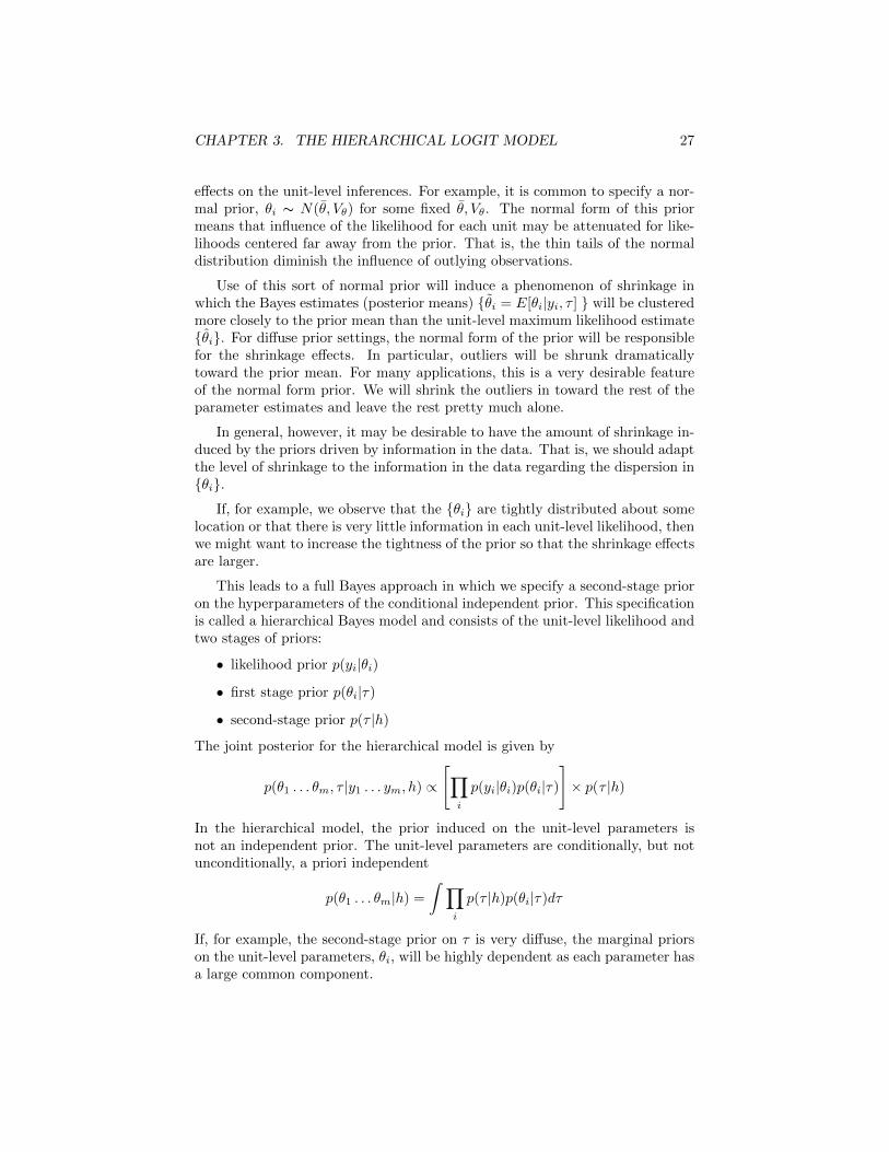
effects on the unit-level inferences. For example, it is common to specify a nor-mal prior, θi ∼ N(θ, Vθ) for some fixed θ, Vθ. The normal form of this priormeans that influence of the likelihood for each unit may be attenuated for like-lihoods centered far away from the prior. That is, the thin tails of the normaldistribution diminish the influence of outlying observations.
Use of this sort of normal prior will induce a phenomenon of shrinkage inwhich the Bayes estimates (posterior means) {θi = E[θi|yi, τ ] } will be clusteredmore closely to the prior mean than the unit-level maximum likelihood estimate{θi}. For diffuse prior settings, the normal form of the prior will be responsiblefor the shrinkage effects. In particular, outliers will be shrunk dramaticallytoward the prior mean. For many applications, this is a very desirable featureof the normal form prior. We will shrink the outliers in toward the rest of theparameter estimates and leave the rest pretty much alone.
In general, however, it may be desirable to have the amount of shrinkage in-duced by the priors driven by information in the data. That is, we should adaptthe level of shrinkage to the information in the data regarding the dispersion in{θi}.
If, for example, we observe that the {θi} are tightly distributed about somelocation or that there is very little information in each unit-level likelihood, thenwe might want to increase the tightness of the prior so that the shrinkage effectsare larger.
This leads to a full Bayes approach in which we specify a second-stage prioron the hyperparameters of the conditional independent prior. This specificationis called a hierarchical Bayes model and consists of the unit-level likelihood andtwo stages of priors:
• likelihood prior p(yi|θi)
• first stage prior p(θi|τ)
• second-stage prior p(τ |h)
The joint posterior for the hierarchical model is given by
p(θ1 . . . θm, τ |y1 . . . ym, h) ∝
[∏i
p(yi|θi)p(θi|τ)
]× p(τ |h)
In the hierarchical model, the prior induced on the unit-level parameters isnot an independent prior. The unit-level parameters are conditionally, but notunconditionally, a priori independent
p(θ1 . . . θm|h) =
∫ ∏i
p(τ |h)p(θi|τ)dτ
If, for example, the second-stage prior on τ is very diffuse, the marginal priorson the unit-level parameters, θi, will be highly dependent as each parameter hasa large common component.
CHAPTER 3. THE HIERARCHICAL LOGIT MODEL 28
The first-stage prior (or random effect distribution) is often taken to be anormal prior. Obviously, the normal distribution is a flexible distribution witheasily interpretable parameters.
The use of a hierarchical model for prediction also highlights the distinctionbetween various priors. A hierarchical model assumes that each unit is a drawfrom a superpopulation or that the units are exchangeable. This means thatif we want to make a prediction regarding a new unit we can regard this newunit as drawn from the same population. Without the hierarchical structure,all we know is that this new unit is different and have little guidance as to howto proceed. These assumptions are all very natural from the point of view ofmarketing practice.
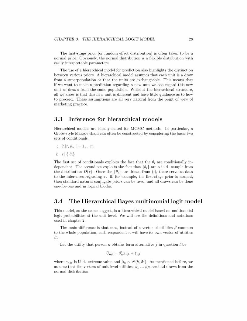
3.3 Inference for hierarchical models
Hierarchical models are ideally suited for MCMC methods. In particular, aGibbs-style Markov chain can often be constructed by considering the basic twosets of conditionals:
i. θi|τ, yi, i = 1 . . .m
ii. τ | { θi}
The first set of conditionals exploits the fact that the θi are conditionally in-dependent. The second set exploits the fact that {θi} are a i.i.d. sample fromthe distribution D(τ). Once the {θi} are drawn from (i), these serve as datato the inferences regarding τ . If, for example, the first-stage prior is normal,then standard natural conjugate priors can be used, and all draws can be doneone-for-one and in logical blocks.
3.4 The Hierarchical Bayes multinomial logit model
This model, as the name suggest, is a hierarchical model based on multinomiallogit probabilities at the unit level. We will use the definitions and notationsused in chapter 2.
The main difference is that now, instead of a vector of utilities β commonto the whole population, each respondent n will have its own vector of utilitiesβn.
Let the utility that person n obtains form alternative j in question t be
Unjt = β′nxnjt + εnjt
where εnjt is i.i.d. extreme value and βn ∼ N(b,W ). As mentioned before, weassume that the vectors of unit level utilities, β1 . . . βN are i.i.d draws from thenormal distribution.

CHAPTER 3. THE HIERARCHICAL LOGIT MODEL 29
This is equivalent to say that the respondents are a random sample of apopulation whose utilities are distributed normally with mean b and covariancematrix W .
Giving βn a normal distribution allows us to speed estimation considerablyby using conjugate priors. We will give details on this later on.
We also give priors to b and W . Suppose the prior on b is Normal. If wehave no prior information on b, which very likely will be the case, we may usea non-informative prior with unboundedly large variance.
We choose to use an inverted Wishart as the prior for W . If we have noprior information, we may choose as parameters K for the degrees of freedomand IK as the scale matrix, where K is the dimension of the parameter spaceand IK is the K-dimensional scale matrix.
A sample of N respondents is observed. For simplicity of exposition wesuppose all people responded to the same number of questions T . The chosenalternatives in all questions for person n are denoted y′n = {yn1, . . . , ynT} andthe choices of the entire sample are labeled Y = {y1, . . . , yn}.
The probability of person n′s observed choices, conditional on the parametersβn, b,W is
L(yn|βn) =∏i
(eβ′nxnyni∑j eβ′nxnj
)The probability not conditional on βn is the integral of L(yn|βn) over all possiblevalues of βn:
L(yn|b,W ) =
∫L(yn|β)φ(βn|b,W )dβn
where φ(βn|b,W ) is the normal density with mean b and variance W .
The posterior distribution of b, W and β1, . . . , βN is by definition
K(b,W, β1 . . . βN |Y ) ∝∏n
L(yn|βn)φ(βn|b,W )k(b,W )
where k(b,W ) is the prior on b and W described earlier: normal for b timesinverted Wishart for W.
Draws from this posterior are obtained through a 3 layers Gibbs sampling.Before describing the layers in detail, we recall three useful Lemmas:
Lemma 3.4.0.1 (conjugate prior for Normal with unknown mean, known vari-ance)
Let the random variable β be distributed normally with unknown mean band known variance σ. Let β1 . . . βN an i.i.d. sample of β and suppose theresearcher’s prior on b is N(β0, S0).
CHAPTER 3. THE HIERARCHICAL LOGIT MODEL 30
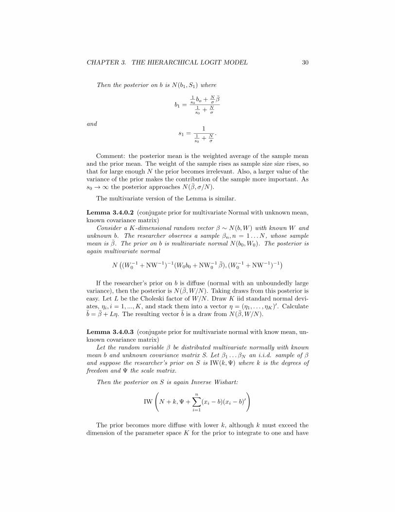
Then the posterior on b is N(b1, S1) where
b1 =1s0bo + N
σ β1s0
+ Nσ
and
s1 =1
1s0
+ Nσ
.
Comment: the posterior mean is the weighted average of the sample meanand the prior mean. The weight of the sample rises as sample size size rises, sothat for large enough N the prior becomes irrelevant. Also, a larger value of thevariance of the prior makes the contribution of the sample more important. Ass0 →∞ the posterior approaches N(β, σ/N).
The multivariate version of the Lemma is similar.
Lemma 3.4.0.2 (conjugate prior for multivariate Normal with unknown mean,known covariance matrix)
Consider a K-dimensional random vector β ∼ N(b,W ) with known W andunknown b. The researcher observes a sample βn, n = 1 . . . N , whose samplemean is β. The prior on b is multivariate normal N(b0,W0). The posterior isagain multivariate normal
N((W−10 + NW−1)−1(W0b0 + NW−10 β), (W−10 + NW−1)−1
)If the researcher’s prior on b is diffuse (normal with an unboundedly large
variance), then the posterior is N(β,W/N). Taking draws from this posterior iseasy. Let L be the Choleski factor of W/N . Draw K iid standard normal devi-ates, ηi, i = 1, ...,K, and stack them into a vector η = (η1, . . . , ηK)′. Calculateb = β + Lη. The resulting vector b is a draw from N(β,W/N).
Lemma 3.4.0.3 (conjugate prior for multivariate normal with know mean, un-known covariance matrix)
Let the random variable β be distributed multivariate normally with knownmean b and unknown covariance matrix S. Let β1 . . . βN an i.i.d. sample of βand suppose the researcher’s prior on S is IW(k,Ψ) where k is the degrees offreedom and Ψ the scale matrix.
Then the posterior on S is again Inverse Wishart:
IW
(N + k,Ψ +
n∑i=1
(xi − b)(xi − b)′)
The prior becomes more diffuse with lower k, although k must exceed thedimension of the parameter space K for the prior to integrate to one and have

CHAPTER 3. THE HIERARCHICAL LOGIT MODEL 31
means. With Ψ = I, where I is the K-dimensional identity matrix, the posteriorunder a diffuse prior becomes IW(K+N, (KI +NS)/(K+N)). Conceptually thisprior is equivalent to the researcher having a previous sample of K observationswhose sample variance was I. As N rises without bound, the influence of theprior on the posterior eventually disappears.
3.4.1 Estimation for the Hierarchical logit model
We choose to use a Gibbs sampler to sample from the posterior. The Gibbssampler has three layers:
1. b|W,β1, . . . , βN . The βn’s constitute a sample ofN realizations from a normaldistribution with unknown mean and known covariance matrix. We cantherefore use lemma 3.4.0.2. If we are using a diffuse prior, the posterior onb is N(β,W/N), where β is the sample mean of the βn’s.
2. W |b, β1, . . . , βN . The βn’s constitute a sample from a normal distributionwith known mean b. Given lemma 3.4.0.3 and our prior on W, the posterioron W is inverted Wishart with K + N degrees of freedom and scale matrix(KI + NS1)/(K + N), where S1 =(1/N)
∑n(βn − b)(βn − b)’ is the sample
variance of the βn’s around known mean b.SS
3. βn|b,W . The posterior for each respondent’s βn, conditional on the observedchoices and the population parameters is
K(βn|b,W, yn) ∝ L(yn|βn)φ(βn|b,W )
It is easy to draw from distributions of layers 1 and 2. However, there is no easyway to draw directly from layer 3 so a MH algorithm is used.
For each βni the MH algorithm operates as follows:
a) Start with a value βin
b) Draw K independent values from a standard normal density, and stack thedraws in a vector labeled η1
c) Create a trial value of βi+1n as βn
i+1= βin+ρLη1, where ρ is a scalar specified
by the researcher and L is the Choleski factor of W . Note that the proposaldistribution is specified to be normal with zero mean and variance ρ2W
d) Draw a standard uniform variable µi+1
e) Calculate the ratio
F =L(yn|βn
i+1)φ(βn
i+1|b,W )
L(yn|βin)φ(βin|b,W )
CHAPTER 3. THE HIERARCHICAL LOGIT MODEL 32
f) If µi+1 6 F , accept βni+1
and let βi+1n = βn
i+1.
If µi+1 > F , reject βni+1
and let βi+1n = βin.
g) Repeat. For high enough i, βin is a draw from the posterior.
In the MH algorithm, the scalar ρ is specified by the researcher. This scalardetermines the size of each jump. Usually, smaller jumps translate into moreaccepts, and larger jumps result in fewer accepts. However, smaller jumps meanthat the MH algorithm takes more iterations to converge and embodies moreserial correlation in the draws after convergence. They optimal acceptance ratefor the MH algorithm is about 0.44 when K =1 and drops toward 0.23 as Krises. See Gelman et al. (1995, p. 335) for details.
The value of ρ can be set by the researcher to achieve an acceptance rate inthis neighborhood, lowering ρ to obtain a higher acceptance rate and raising itto get a lower acceptance rate. In fact, ρ can be adjusted within the iterativeprocess.
The researcher sets the initial value of ρ. In each iteration, a trial βn isaccepted or rejected for each sampled n. If in an iteration, the acceptance rateamong the N observations is above a given value (say, 0.33), then ρ is raised. Ifthe acceptance rate is below this value, ρ is lowered. The value of ρ then movesduring the iteration process to attain the specified acceptance level.
To sum up, we’ll write again in a more concise form the estimation procedure.
We start with any initial values b0,W 0, β01 . . . β
0N . The t-th iteration of the
Gibbs sampler consists of these steps:
1. Draw bt from N(βt−1,W t−1/N) where βt−1
is the mean of the βt−1n
2. Draw W t from IW(K +N, (KI + NSt−1)/(K +N)), where
St−1 = Σn(βt−1n − bt)(βt−1n − bt)′/N ˆ
3. For each n draw βtn using one iteration of the MH algorithm previouslydescribed, starting from βt−1n and using the normal density φ(βn|bt,W t)
These three steps are repeated for many iterations. The resulting values con-verge to draws from the joint posterior of b,W , and β1, . . . , βN . Once theconverged draws from the posterior are obtained, the mean and standard devi-ation of the draws can be calculated to obtain estimates and standard errors ofthe parameters.
The Gibbs sampler converges, with enough iterations, to draws from thejoint posterior of all the parameters. The iterations prior to convergence areoften called burn-in. Unfortunately, it is not always easy to determine whenconvergence has been achieved. In practical applications, a sufficiently highnumber of iterations is performed prior assuming convergence.
CHAPTER 3. THE HIERARCHICAL LOGIT MODEL 33
During burn-in, the researcher will usually be able to see the draws trending,that is, moving toward the mass of the posterior. After convergence has beenachieved, the draws tend to move around (traverse) the posterior. The drawsfrom Gibbs sampling are correlated over iterations even after convergence hasbeen achieved, since each iteration builds on the previous one. This correlationdoes not prevent the draws from being used for calculating the posterior meanand standard deviation, or other statistics. However, the researcher can reducethe amount of correlation among the draws by using only a portion of the drawsthat are obtained after convergence. For example, the researcher might retainevery tenth draw and discard the others, thereby reducing the correlation amongthe retained draws by an order of 10. A researcher might therefore specify atotal of 20,000 iterations in order to obtain 1000 draws: 10,000 for burn-in and10,000 after convergence, of which every tenth is retained.
Succinct restatement of the model
Utility:Unjt = β′nxnjt + εnjt
εnjti.i.d. extreme value
βn ∼ N(b,W )
Observed choice:
ynt = i if and only if Unit > Unjt∀j 6= i
Uninformative priors:k(b,W ) = k(b)k(W )
wherek(b) ∼ N(b0,W0) with very large variance
k(W ) ∼ IW(K, I)
Conditional posteriors:
K(βn|b,W, yn) ∝∏i
(eβ′nxnyntt∑j eβ′nxnj
)φ(βn|b,W )∀n
K(b|W,β1, . . . , βN ) ∝ N(β,W/N) where β = Σnβn/N
K(W |b, β1, . . . , βN ) ∝ IW(K +N,KI +NS
K +N) where S = Σn(βn − b)(βn − b)′/N
Chapter 4
Optional features
Optional features are for us all the extra services or products that can be pur-chased in addition to a core product.Examples of optional features include extras in automotive industry, addition toservice plans in telecommunication industry, extra warranty coverage in manyelectronics products and many more.
4.1 Business perspective
From a seller’s point of view, offering certain feature as optional has great ad-vantages.First and foremost, it is a simple way to enrich one’s portfolio.Offering a new feature as an option can make the product appealing to morecustomers without the risk of alienating the current ones, as the product theyknow and like is still available to them.
Offering optional features can increase the out-of-pocket expense. Further-more, optional features can be used to break psychological price barriers. Ifthere is a price barrier at, say, 100 euro, the core product could be offered for99 euro and a interesting optional feature could be offered for a price way lowerthan its market value - just a few euro.At this point, being already over the barrier price of 100 euro, a customercould buy other more expensive options, therefore increasing his/her total out-of-pocket expense.
It is known from marketing literature [1] that the offering of certain optionsand services makes the product more interesting even for people that are notgoing to purchase those options.We will call this Halo Effect. In a rather extreme case, a company may want tooffer and advertise an option that almost no customer is actually ever going to

CHAPTER 4. OPTIONAL FEATURES 35
Figure 4.1: Optional features for Vodafone mobile contracts
buy but that makes the product look more interesting.This may be the case for some advanced technological features: advertisingwould be focused on the new cutting-edge technological feature, even if veryfew people will want to pay for it.
The example shown in figure 4 shows other interesting properties of optionalfeatures. Customers had the possibility to upgrade their contract any time. It ispossible that they gave value to the presence of mobile connectivity, even whennot using it right away, because they were thinking of using it in the future.When it is possible for the customer to buy an optional feature in a second pur-chase, the simple presence of an optional feature can give value to the product:it gives the customer the opportunity to upgrade at a later stage. This is likesaying there is a value in opportunity.
We can see this structure in services where the core feature is usually verycheap (or even free) and that offer the possibility to expand for a price.For example, VOIP clients like Skype usually offer free client-to-client calls and

CHAPTER 4. OPTIONAL FEATURES 36
chat services.They offer paid packages for calls to telephone numbers etc. that can be boughtat any moment. Therefore, people are mainly convinced to use the client (coreproduct) because of the possibility to expand (call plans).Also, there is a lock-in effect: when one’s contact use a certain client chatsystem, it is convenient to keep on using the same client.
A completely different example of optional features is the accessories soldwith Dell computers.When buying a Dell, it is possible to customize the specifications of the hard-ware. This is called Build-your-own or BYO model. Also, it is possible to buyother accessories such as printers, scanners, laptop bags, speakers etc.All those optional features can be obtained at a later stage from other providers.Since they are usually compatible with all pc’s, offering them probably doesn’tprovide any halo effect. Therefore the main interest of Dell is to have a range ofoptions that customers will buy at the moment of purchase of the core product.
In service markets like insurance, telecom, finance etc. it is generally alwayspossible to upgrade one’s contract selecting optional features at a later stage.An example of optional feature that can’t be bought at a second moment is anextension of the warranty period of a product.We think that the halo effect is sensibly stronger for features that can’t bepurchased in a second moment, but we didn’t investigate in this direction andas far as we know there is no material on this topic.
From the customer’s point of view, options are welcome, too.Options give the sensation of creating a product that is truly fitting one’s needs.Also, they can be perceived as a saving: the customer only pays for what he/shereally needs and nothing more.
In some extreme case, the choice of options is so wide that a customer canbuild his/her own product from scratch. This is the case of the BYO (Buildyour own) products, or mass customization products.In this case, the customer gets the idea that the resulting product is going tobe his/her very own, tailor made according to his/her tastes.
Offering optional features has pitfalls, too.Offering many options can make a product very customizable to the needs ofthe buyer, but it can also make the choice decision long and complex.It is a well established fact, both in practice and literature [1], that optionalfeatures can lead to a product being perceived as complicated. This is notonly a matter of quantity but also of quality: even when offering a very limitednumber of options, some of them may take a considerable effort to be evaluated.The result is that the core product is deemed as less attractive: customers mayswitch to other products that satisfy their needs and are less complicated toevaluate.
A common solution to this problem is to offer only a limited number ofoptional features bundled in a package. This makes the evaluation easier, but
CHAPTER 4. OPTIONAL FEATURES 37
of course it hinders one of the greatest advantages of optional features: thepossibility for the customer to buy just what he/she needs and nothing more.
It is also possible to use a mixed strategy, offering single options and bundles.This is the case of, for example, fast food restaurants. It is possible to buy amenu (a bundle) or just fries and a soft drink (some of the features composingthe bundle).In this case, when customers can see the prices of the single parts of the bundle,they expect a discount on the total price.
4.2 Summary of business questions
The basic business question when dealing with optional feature is What is theoptimal set of options we should offer?
We can split this very wide question in more precise sub-questions:
• What is the optimal number of options to offer?
• How many people are going to buy a given option?
• Do the options add value to the core product?
• Does the option X make the product complicated?
• Has the option X a halo effect?
• Do people buy certain options together? Should we bundle them?
These are very different questions. We will provide a way to answer most ofthem by using the powerful tool of choice-based conjoint models.
4.3 Scope of our analysis
We will limit our analysis to products that offer a limited number of options. Inother words, we are not going to consider BYO products or other products thatcan’t be easily evaluated at once by the customer. This is because of theoreticaland practical reasons related to our choice of the conjoint methodology.It is a well established fact that conjoint analysis yields good results only if alimited number of attributes per product are shown. When confronted with toocomplicated products, respondents tends to use simplification strategies and,even worse, get tired more easily providing senseless answers. In other terms,conjoint is appropriate only for studying products that a customer can evaluatein their integrity.
This is not a limitation of this technique. This is because of the way weactually evaluate products: when choosing between a set of products whosefeatures we can actually retain in our minds, we can evaluate their value very
CHAPTER 4. OPTIONAL FEATURES 38
easily. Therefore we use a choosing model similar to the use described by con-joint. When considering extremely complicated products (like BYO products)the main mental task we perform is evaluating the value of a single of thoseproducts.
In simpler words, it is very easy to tell between two candy bars which one welike more, because we can have a clear image in our mind of what their featuresare. When having to select between two offers from different brands of BYOmotorcycle from scratch (as Harley Davidson used to offer) we are not able totell easily which one is better. We actually spend much of our time choosingthe options of one of the two companies, instead of deciding which of the two isbetter. In this sense, forecasting BYO offer we are going to take is not a goodquestion for a conjoint study: most of the mental work is evaluating one of theproducts, rather than the tradeoffs between one product and the others.
4.4 Methodology
In this section we propose a methodology that is able to answer the businessquestions put forth in section 4.2. The proposed methodology has been exten-sively tested in simulations and then applied to data from a real survey.
To find a way to estimate utilities for optional features we start with creatinga model for the respondent choice behavior.
The usual conjoint model is based on the fact that customers can keep inmind all relevant aspects of offered products and they can assign a utility toeach of them. Their final choice is done by considering at once all the productsand selecting one in a way proportional to their utilities. We are going to modifythe normal conjoint model to account for optional features.
4.5 Questionnaire structure
Just as in standard conjoint studies, our analysis will be based on questionnairesanswers.We will show a certain number of core products and options to all customersand ask them to choose one core product and some of its options.In normal conjoint studies what we observe is a choice of a product in a groupof n.In an optional feature study we observe the choice of a product and of some ofits options. We don’t ask the respondent to state anything about the optionspresent in the other products.The respondent’s task is very similar to an actual purchase. Not asking any-thing about the other product options we loose a great amount of data but weretain realism in tasks, the most important feature of usual conjoint tasks.
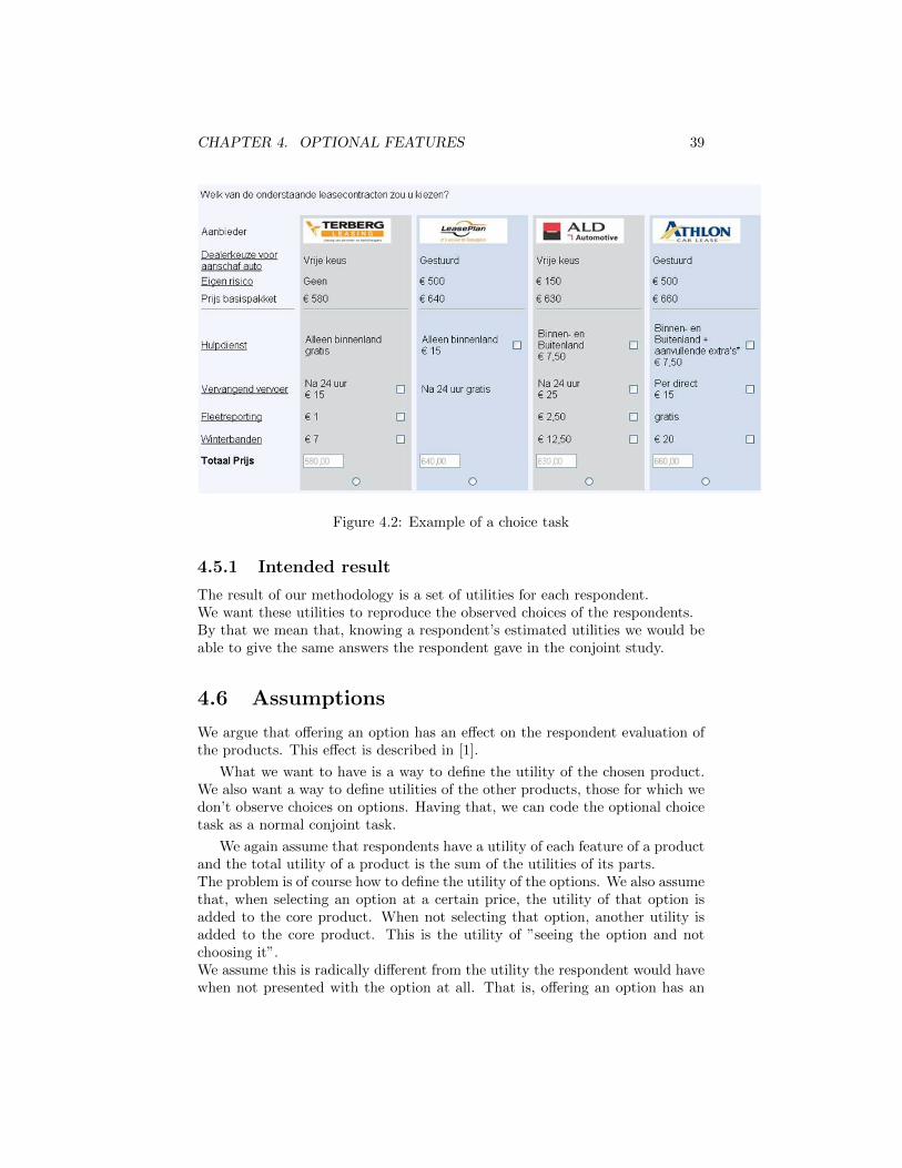
CHAPTER 4. OPTIONAL FEATURES 39
Figure 4.2: Example of a choice task
4.5.1 Intended result
The result of our methodology is a set of utilities for each respondent.We want these utilities to reproduce the observed choices of the respondents.By that we mean that, knowing a respondent’s estimated utilities we would beable to give the same answers the respondent gave in the conjoint study.
4.6 Assumptions
We argue that offering an option has an effect on the respondent evaluation ofthe products. This effect is described in [1].
What we want to have is a way to define the utility of the chosen product.We also want a way to define utilities of the other products, those for which wedon’t observe choices on options. Having that, we can code the optional choicetask as a normal conjoint task.
We again assume that respondents have a utility of each feature of a productand the total utility of a product is the sum of the utilities of its parts.The problem is of course how to define the utility of the options. We also assumethat, when selecting an option at a certain price, the utility of that option isadded to the core product. When not selecting that option, another utility isadded to the core product. This is the utility of ”seeing the option and notchoosing it”.We assume this is radically different from the utility the respondent would havewhen not presented with the option at all. That is, offering an option has an
CHAPTER 4. OPTIONAL FEATURES 40
impact of the utility of the product, even for people that don’t select it. This isin accordance to marketing theory.
If the chosen product comes with option A at price p1, and option A isselected, the utility of the chosen product will be the utility of its core featureplus the utility of ”having A at price p1”. If option A is not selected, the utilityof the chosen product will be the utility of its core features plus the utility of”not having A”.If option A is not offered in that product, the total utility is the utility of thecore product plus utility of ”A not offered”.
That is, the respondents obtain different utilities for selecting an option atdifferent prices. Of course we can imagine that selecting A at a price of 10 willyield lower utility than selecting A at a price of 5.
On the other hand, the utility that we obtain when not selecting an optiondoes not depend on the price at which said option was presented.This is a very important concept: we have different utilities for showing anoption at different prices, but one utility for not selecting the option, no matterwhat the price shown.
Also, we assume that people perceive in a different way not being offered anoption and being offered an option and deciding not to choose it. In simplerwords, the act of offering an option has consequences in the product evaluation,be that option selected or not.The fact that the respondents sees the option is important. The non chosenoption still lingers in the mind of the respondent, therefore changing its percep-tion of the whole product.In particular, we already know that options can make a product complex or canhave a halo effect. We think that, when the utility of the Not Chosen level ofan option is higher than the Not Offered level, the option gives a halo effect.When the opposite happens, the option is making the product complicated.
Having defined utilities that respondents get from selecting or not an option,we have to decide how those utilities influence the choice of an option. Weconsidered two models: first choice and share of preference. In the first model,an option is selected with probability 1 if its utility is higher than the utilityfor not selecting it. In the second model, an option is selected with probabilityproportional to the exponential of its utility.
4.7 Simulations
We developed our methodology by performing estimation on simulated datasets.To simulate datasets, we generate a questionnaire using Sawtooth SSIWeb.Then we generate utilities for the respondents by sampling from a multivari-ate normal with given mean and covariance matrix (as described in the conjointmodel). We refer to these utilities as ”real utilities”. We generated three differ-ent sets of utilities to use in the simulations. We use the real utilities to generate
CHAPTER 4. OPTIONAL FEATURES 41
answers to the questionnaires using different procedures. In this process we adddifferent kind of random error to further test the robustness of the algorithm.
4.7.1 Answer generation procedures
No Error In the No Error scenario, real utilities are used to generate answers.An option is chosen with probability 1 if its utility is higher than the utility ofthe Not Chosen option (perfect option choice). The product with the highestutility is chosen with probability 1 (perfect product choice).
Error 1 In the Error1 scenario, options are again chosen basing on thereal utilities (perfect option choice). Products are chosen with probabilitiesproportional to the exponential of their utilities. This is a type I extreme valueerror, arising from a Gumbel distribution. This is also the error form specifiedin the conjoint model.
Error 2 In the Error2 scenario, also options are chosen with Gumbel errors.
Using these procedures we generate answers to the questionnaires. As in aconjoint experiment, the answer is the choice of one product and some of itsoptions. In one case, we have an extra procedure that relaxes this assumption:
Perfect choice on all options In this scenario we observe option selectionalso in the non-chosen product.
This last procedure is mostly of theoretic interest since asking respondentsto state anything about non-selected products would destroy the realism of thechoice task.Respondent are very keen on selecting the best product in choice tasks, as theydo in life, but would probably give non-realistic results when selecting optionsof the non-chosen products. They have no interest in evaluating carefully whatthey are not interested in.
4.7.2 Set of utilities
All set of utilities feature utilities for 300 respondents. For each respondent wegenerate utilities for 4 attributes each with 7 levels, one of which represents theNot Chosen level. Each respondent answers to 12 fully-randomized questions.These dimensions are similar to the ones of a middle-sized study.
No heterogeneity In this set all respondents have similar utilities. Thismeans that they will tend to select or not to select the same option. This meansthat, when using perfect option choice, average choice rate for an option leveltends to be either 1 or 0. This set was used as a first filter: if an estimationprocedure performs poorly on this set it is not suitable for use. The covariancematrix is diagonal, 1*I
Heterogeneity 1-middle heterogeneity In this realistic set respondentshave different preferences for options. When using perfect options choice, most

CHAPTER 4. OPTIONAL FEATURES 42
option levels have average choice rates among all respondents that don’t collapseto 0 or 1. The covariance matrix is diagonal, 3*I
Heterogeneity 2-high heterogeneity Similar to heterogeneity 1. Thereis even more variety between respondents. The covariance matrix is diagonal,5*I
4.8 Estimation procedures
Options coding If option j is chosen in the selected product, we set the valueof the same option in the other products as if they were selected.If option j is not chosen in the selected product, we set its value as Not Chosenand we do the same for the other products.If an option was Not Present (i.e. for that product it was not possible to selectit), it is always coded as Not Present.
Table 4.1: Example of a choice task. The respondent chose product 2, its firstoption but not the second one.
Product 1 Product 2 Product 3 Product 4
Core Attribute 1 A1 A2 A1 A2Core Attribute 2 B1 B2 B2 B1
Core Price (Euro) 10 15 12 20Option 1 M@10 Euro M@15 Euro M@8 Euro M@15 Euro
Chosen Y/N XOption 2 N@10 Euro N@15 Euro N Not Present N@10 Euro
Chosen Y/N ×Choice •
Table 4.2: Options coding: the selection
Product 1 Product 2 Product 3 Product 4
Core Attribute 1 A1 A2 A1 A2Core Attribute 2 B1 B2 B2 B1
Core Price (Euro) 10 15 12 20Option 1 M@10 Euro M@15 Euro M@8 Euro M@15 Euro
Chosen Y/N X X X XOption 2 N@10 Euro N@15 Euro N Not Present N@10 Euro
Chosen Y/N × × × ×Choice •
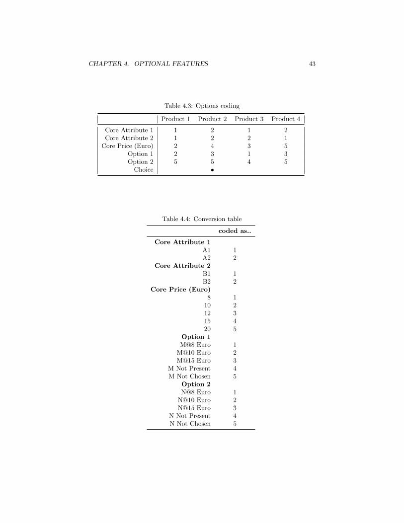
CHAPTER 4. OPTIONAL FEATURES 43
Table 4.3: Options coding
Product 1 Product 2 Product 3 Product 4
Core Attribute 1 1 2 1 2Core Attribute 2 1 2 2 1
Core Price (Euro) 2 4 3 5Option 1 2 3 1 3Option 2 5 5 4 5
Choice •
Table 4.4: Conversion table
coded as..
Core Attribute 1A1 1A2 2
Core Attribute 2B1 1B2 2
Core Price (Euro)8 1
10 212 315 420 5
Option 1M@8 Euro 1
M@10 Euro 2M@15 Euro 3
M Not Present 4M Not Chosen 5
Option 2N@8 Euro 1
N@10 Euro 2N@15 Euro 3
N Not Present 4N Not Chosen 5
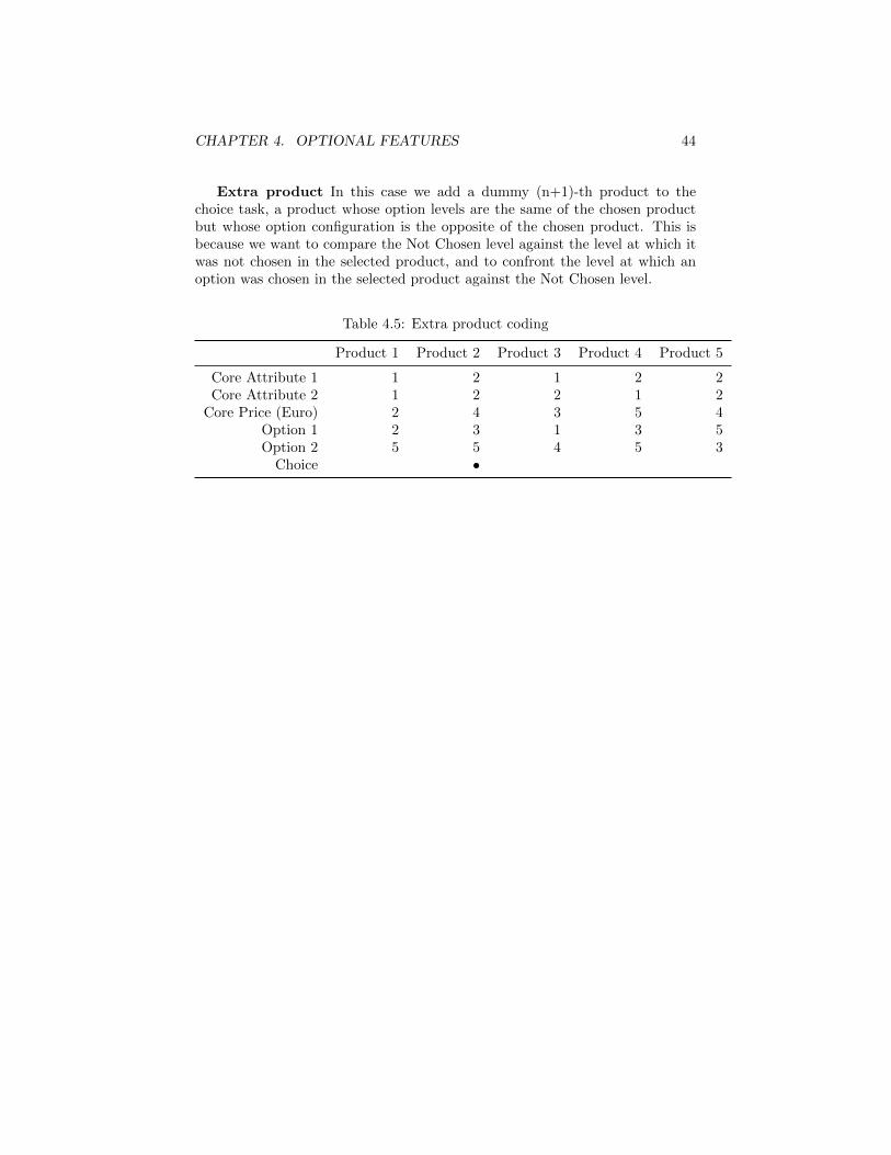
CHAPTER 4. OPTIONAL FEATURES 44
Extra product In this case we add a dummy (n+1)-th product to thechoice task, a product whose option levels are the same of the chosen productbut whose option configuration is the opposite of the chosen product. This isbecause we want to compare the Not Chosen level against the level at which itwas not chosen in the selected product, and to confront the level at which anoption was chosen in the selected product against the Not Chosen level.
Table 4.5: Extra product coding
Product 1 Product 2 Product 3 Product 4 Product 5
Core Attribute 1 1 2 1 2 2Core Attribute 2 1 2 2 1 2
Core Price (Euro) 2 4 3 5 4Option 1 2 3 1 3 5Option 2 5 5 4 5 3
Choice •

CHAPTER 4. OPTIONAL FEATURES 45
4.9 Measures of fit
To measure the fit of the model with the data we will mostly look at two kindsof indicators:-utilities, at a respondent level-option choice probability, on a aggregate levelIn the first case we consider the questions given to the respondent, his/her an-swers and we see if the respondent’s utilities match the information given in theanswers.That is, we see if the utility of an option level that was chosen in the question-naire is higher than the No Choice utility.We are not interested in recovering the real utility values but rather to find util-ities that reproduce the observed choices. This is the most important measureof fit.Of course, since each respondent only sees some of the possible options level inhis/her questions, for some option levels the information will be borrowed fromthe whole population.In the second case we consider each respondent’s utilities and we check whatoption would be chosen basing on these. We do the same with the real utilitiesand we count the number of times the choice is the same.
This is called Option Count and is calculated over all options taken together.We also consider the percentage of choice for a single option.Again, we are not interested in recovering perfectly the observed probabilitiesbut rather to see if the differences are going in a certain direction or if the prob-abilities collapse to 0 or 1.It may be the case that the Option Count gives good results but only becauseall choice probabilities collapse to 1. In this last case, the fit of the model isindeed very poor.Our aim is not to be able to predict correctly the choice of every single optionbut rather to have a set of utilities reproducing the observed choices.In this sense, the value of the prediction choice is not a goal but is anyway prettyimportant to assess the goodness of the model.Also, we look at the PCT to see how well the model fit the data. When con-sidering this measure we must consider that adding an extra product increasesartificially the PCT, since it is a very unlikely product to be chosen.
4.10 Simulation results
We report the results of the simulations. The tables containing the estimatedutilities can be found in the appendix. We advise the readers to look carefully atthe questionnaires and the estimated utilities at a respondent’s level to considerwhich estimation method is better.
Scenario name: heterogeneity 1, extra product, no errorFolder: het1 Number of iterations: 20k

CHAPTER 4. OPTIONAL FEATURES 46
Iteration Jump Size Acceptance Pct. Cert. RLH Avg Var Parameter RMS20000 0.169 0.277 0.957 0.933 5.543 8.129
Options prediction percentage: 86/Exact options choice percentages:Estimated options choice percentages:Considerations:
Scenario name: heterogeneity 1, extra product, error 1 Folder:het1E Number of iterations: 20k
Iteration Jump Size Acceptance Pct. Cert. RLH Avg Var Parameter RMS20000 0.132 0.293 0.781 0.703 5.715 5.693Estimated options choice percentages: 86/Considerations:Scenario name: heterogeneity 1, extra product, error 2 Folder:
het1E2 Number of iterations: 20kIteration Jump Size Acceptance Pct. Cert. RLH Avg Var Parameter RMS
20000 0.123 0.337 0.277 0.312 3.473 2.325Estimated options choice percentages: 54/Considerations:Scenario name: heterogeneity 1, extra product, error 2, perfect
choice in all optionsFolder: het1E2perfchoice Number of iterations: 20kIteration Jump Size Acceptance Pct. Cert. RLH Avg Var Parameter RMS
20000 0.096 0.313 0.611 0.535 9.960 6.188Estimated options choice percentages: 85/Considerations:Scenario name: heterogeneity 1, extra info, no error Folder: het1Eextrainfo
Number of iterations: 20kIteration Jump Size Acceptance Pct. Cert. RLH Avg Var Parameter RMS
20000 0.102 0.343 0.948 0.925 15.831 7.824Estimated options choice percentages: 95/Considerations:Scenario name: heterogeneity 1, extra info, error 1Folder: het1Eextrainfo Number of iterations: 20kIteration Jump Size Acceptance Pct. Cert. RLH Avg Var Parameter RMS
20000 0.104 0.350 0.801 0.736 7.595 5.231Estimated options choice percentages: 90/Considerations:Scenario name: heterogeneity 1, options coding, error 1 Folder:
het1nofifth Number of iterations: 20kOptions prediction percentage: 79/Exact options choice percentages:Iteration Jump Size Acceptance Pct. Cert. RLH Avg Var Parameter RMS
20000 0.139 0.350 0.952 0.936 6.620 7.734Estimated options choice percentages:Considerations:Scenario name: heterogeneity 1, perfect choice, no error

CHAPTER 4. OPTIONAL FEATURES 47
Folder: het1perfchoice Number of iterations: 20kIteration Jump Size Acceptance Pct. Cert. RLH Avg Var Parameter RMS
20000 0.087 0.290 0.895 0.845 7.071 5.138Estimated options choice percentages: 76/Considerations:Scenario name: heterogeneity 2, extra product, no errorFolder: het2 Number of iterations: 20kIteration Jump Size Acceptance Pct. Cert. RLH Avg Var Parameter RMS
20000 0.125 0.303 0.946 0.917 6.753 6.924Estimated options choice percentages: 77/Considerations:Scenario name: heterogeneity 2, extra info, no errorFolder: het2extrainfo Number of iterations: 20kIteration Jump Size Acceptance Pct. Cert. RLH Avg Var Parameter RMS
20000 0.129 0.290 0.925 0.898 6.416 6.621Estimated options choice percentages: 77/Considerations:Scenario name: heterogeneity 2, options coding, no errorFolder: het2nofifth Number of iterations: 20kIteration Jump Size Acceptance Pct. Cert. RLH Avg Var Parameter RMS
20000 0.121 0.300 0.930 0.908 5.821 6.076Estimated options choice percentages: 66/Considerations:Scenario name: heterogeneity 2, perfect choice, no errorFolder: het2perfchoice Number of iterations: 20kIteration Jump Size Acceptance Pct. Cert. RLH Avg Var Parameter RMS
20000 0.080 0.260 0.901 0.853 7.580 5.010Estimated options choice percentages: 74/Considerations:Scenario name: heterogeneity 1, perfect choice, error 1Folder: het1Eperfchoice Number of iterations: 20kIteration Jump Size Acceptance Pct. Cert. RLH Avg Var Parameter RMSEstimated options choice percentages:Considerations:Scenario name: no heterogeneity, extra info, no errorFolder: nohetextrainfo Number of iterations: 20kIteration Jump Size Acceptance Pct. Cert. RLH Avg Var Parameter RMS
20000 0.169 0.220 0.880 0.841 5.229 7.331Estimated options choice percentages: 86/Considerations:Scenario name: no heterogeneity, options coding, no errorFolder: nohetnofifth Number of iterations: 20kIteration Jump Size Acceptance Pct. Cert. RLH Avg Var Parameter RMSEstimated options choice percentages:Considerations:Scenario name: no heterogeneity, perfect choice, no error

CHAPTER 4. OPTIONAL FEATURES 48
Folder: het2 Number of iterations: 20kIteration Jump Size Acceptance Pct. Cert. RLH Avg Var Parameter RMS
20000 0.140 0.307 0.917 0.876 6.457 5.912Estimated options choice percentages: 59/Considerations:Scenario name: no heterogeneity, extra product, no errorFolder: nonhet1 Number of iterations: 20kIteration Jump Size Acceptance Pct. Cert. RLH Avg Var Parameter RMS
20000 0.108 0.277 0.972 0.957 71.650 20.724Estimated options choice percentages: 94/Considerations:
4.11 Overview of results
Without adding an extra product the model gives quite bad results, especiallyin the options count of dataset with heterogeneity. This is because the value ofthe Not Chosen option is always senseless as this option level is never confrontedagainst the other levels. This is the reason why we decided to modify the optionscoding model to confront the not chosen level against other levels.
When adding the extra product, the model gives acceptable results. Theoption count and the RLH are sufficiently high; the probabilities of choice tendnot to collapse to 0 or 1 although they tend to be quite far from the real ones.In particular, we notice that not all of the information from a single respondentis used.Observing the utilities on a respondent’s level, we see that the model tends toborrow too much from the whole population even when there is valuable infor-mation in the answers.This is especially true when a respondent tends not to choose many levels of agiven option.In this case, each of them appears very few times in the respondent question-naire.For example, if a respondent only chooses level 1 of option A, most of his/hercoded answers will look something like:
Level A of selected product: NCLevel A of non-selected products: NC, NC, NCLevel A of extra product: A2
when the selected product had a level different from A1 in option A.
Only when level A1 is present in the selected product, the coding will looksomething like:
Level A of selected product: A1Level A of non-selected products: A2, A4, A5
CHAPTER 4. OPTIONAL FEATURES 49
Level A of extra product: NC
Let’s say that the chosen product features level A1 only once or twice out of 12questions.
Even if this respondent shows a clear preference of level A1 over the otherlevels of option A, we are not able to see that from the coding of the question-naire: level A1 is almost never shown in the same question as levels A2..A5.Also, the latter don’t appear as often as they should: most of the time, onlyonce per question!
There is an excessive presence of the Not Chosen level, hence skewing thequestionnaire. The algorithm therefore has little information about the nonchosen levels and tends to borrow more from the sample. This leads to anoverestimation of choice probabilities.
To solve this problem we choose to rebalance each respondent coding byadding extra questions in which levels A1..A5 are shown.This is a better solution than just setting the parameters to give a better fitat a respondent’s level. In case of outliers, their utilities wouldn’t be shrunktowards the mean, which is something we want.We want to borrow less from the sample only for those respondents who areconsistent in their answers: therefore we add extra questions only for some ofthe respondents.This gives us control on the level of fit we want for each respondent.
The perfect choice model doesn’t give a sensibly better fit apart from onecase which we will comment later. This is because, just as the base model, thismodel features the winning product, its opposite and four out of all the possibleconfigurations of the other products.The fact that results are not so better makes us think that a iterative model inwhich utilities are estimated many times and option choices in the non chosenproduct are changed after each estimation will not yield sensibly better results.In particular the perfect choice model performs poorly in a low heterogeneityscenario. The problem is similar to the one explained before but even moreextreme: if many levels of an option are not chosen, now they don’t ever appear,not even against the levels of a chosen option. This leads to borrowing a lotfrom the sample.
We analyzed data collected on options. In the leaseplan study, we wereable to see that respondents are extremely consistent with their choices. Whenselecting an option for a given price in a question, they tend to repeat the samechoice in the other questions.This lead us to the assumption that respondents use a first choice model whenchoosing options.If they were using a share of preference model, the choice for a single optionlevel would not be consistent from question to question.
Of course, this may not always be the case. There are studies where theoption choice was not always consistent.

CHAPTER 4. OPTIONAL FEATURES 50
We assume that, when inconsistencies arise, they can be explained by price-based interaction.One such interaction could be a budget constraint: an option level that wasselected in the previous questions is not selected now because the price of thecore product is already too high.The existence of budget constraints has been observed in numerous studies.Instead of an actual budget to spend, we can think of this as the maximumamount a respondent wants to spend when buying a product of a certain class.
We will experiment price interactions when studying bundles, in the bundleschapter.
Adding Gumbel errors in the product choice influence only slightly the good-ness of fit. The estimation at respondent level is equally good.This is a very good result, since Gumbel errors are the errors specified in theconjoint model.
Adding Gumbel errors also in the options choice has an extremely negativeinfluence on the goodness of fit. Also, the option count gives very bad results.Anyway, when price interactions are not present the choice of options tends tobe very consistent. This is what we observed in the Optional Features study,the topic of the next chapter.
Since a different price is shown for each single option, we can imagine thecustomers to be extremely price sensitive and so to always choose the sameoptions.This lead us to think that type I extreme value errors are not the best to describethe choice of a single option. The strange thing is that in perfect choice modelwith Gumble errors on products and options, the fit is quite good. No optionprobability ever collapse to 0 or 1 and their values are actually quite close to thereal ones. This may be because, in a high heterogeneity scenario, adding errorsin option choice smoothes a lot choice probabilities, avoiding extreme values like0 or 1. This may explain why the fit is not so great (just a value of about 6)given this great ability to predict options, but it needs more investigation.
In general, the model gives perfect results in the option count when there islittle heterogeneity. This is not a good result per se, but is a good test for themodel.In case of more heterogeneity, we can see the option count gives good resultsand the aggregate choice probabilities, although not numerically correct, don’tcollapse to 0 or 1.It seems tough that most probabilities are overestimated.This is because some levels may appear very few times in a respondent’s an-swers, as they are replaced by the Not Chosen level. This is partially correctedby adding dummy questions for each respondent. These questions don’t addexternal information and they rebalance the questionnaire against the excessivepresence of Not Chosen levels.
CHAPTER 4. OPTIONAL FEATURES 51
4.12 Conclusions
The simulation results suggest that the best methodology for no error and error1 scenarios is the Extra Information methodology.This methodology leads to utilities that truly match the observed respondent’schoices.All the information given by the respondents is used and the results mirror thisfact.
Interestingly, knowing the real option configuration in the other productsdoesn’t help the estimation procedure. Knowing the choice of options in theother products is pretty much all the information we would be able to get fromeach respondent in an ideal situation. It is good that the Extra Informationmethodology performs almost as good as if we had this information.
When adding Gumbel errors in the choice of options the results are muchworst. We can ask ourselves if adding those errors is really realistic. Whenanalyzing the Leaseplan study data, we were able to see a striking level ofconsistency in the respondents’ behavior. Therefore, we think adding Gumbelerrors in the choice of options makes the model unrealistic.
Being satisfied with the simulation results, we proceed to use our methodol-ogy on real data.
Chapter 5
Optional features study
This market research study was conducted by SKIM for a car leasing company.The aim of the study was to evaluate and optimize the portfolio of contractsthis company was offering.The study took place in April 2008.The name of the company requesting the study and other sensitive data in thestudy have been obscured. The data reprinted here uses fictional names in lieuof the original ones and the names of attribute and levels have been modified.
5.1 Study description
For our purposes, the most interesting part of the study is a series of choicetasks where respondents have to select option.
In each question four products were offered and four options per productwere presented.In each screen the same group of four options was presented for all products.Of course they could differ in level or price.In total, the four options were chosen from a set of 8 options.
The number of respondents was 229. Each respondent was responsible forthe leasing decision in his/her company.They were divided in three groups according to the fleet size of their company:
• Group 1: 1-24 cars, 110 respondents
• Group 2: 25-99 cars, 71 respondents
• Group 3: 100+ cars, 48 respondents.
The data was collected via web.

CHAPTER 5. OPTIONAL FEATURES STUDY 53
Figure 5.1: Screenshot of a choice task with options. The brand names werehidden on request of SKIM.
5.1.1 Description of the attributes and levels
Attributes and levels of the core product:
Brand: seven brands of companies active in the fleet leasing industry. Wedo not report the name of the brands, as requested by SKIM. Dealerkeuzevoor aanschaf auto: Vrije keus, Gestuurd.Gestuurd onderhoud: Ja, Nee, Ja, met haal- en brengservice.Eigenrisiko: Geen, 150, 500.Contact leasemaatschappij: Via algemene desk, Via vast aanspreekpuntbinnendienst,Via vast aanspreekpunt binnendienst + account managerMeer/minder km prijs: (minderkm 5 cent, meerkm 7 cent), (minderkm 0cent, meerkm 10 cent), (minderkm 10 cent, meerkm 10 cent).Prijs (Euro): 560, 580, 600, 620, 630, 640, 650, 660, 670, 680, 700, 720, 740.
Attributes and levels of the optional features:
Fleetreporting: Niet mogelijk, gratis, Euro 1, Euro 2,50, Euro 5, Not chosenWinterbanden: Niet mogelijk, gratis, Euro 7, Euro 12,50, Euro 20, Not cho-senKVT regeling: Niet mogelijk, gratis, Euro 1, Euro 2,50, Euro 5, Not chosen.SVI: Geen, Nationaal gratis, Nationaal Euro 3, Nationaal Euro 6, NationaalEuro 10, Internationaal gratis, Internationaal Euro 3, Internationaal Euro 6,
CHAPTER 5. OPTIONAL FEATURES STUDY 54
Internationaal Euro 10, Nationaal + wasmodule gratis, Nationaal + wasmod-ule Euro 3, Nationaal + wasmodule Euro 6, Nationaal + wasmodule Euro 10,Internationaal + wasmodule gratis, Internationaal + wasmodule Euro 3, In-ternationaal + wasmodule Euro 6, Internationaal + wasmodule Euro 10, Notchosen .Afkoop inleverschade: Niet mogelijk, gratis, Euro 5, Euro 15, Euro 25, Notchosen.Vervangend vervoer: Geen (geen uitbreiding mogelijk), Per direct gratis,Per direct Euro 15, Per direct Euro 25, Na 24 uur gratis, Na 24 uur Euro 15,Na 24 uur Euro 25, Not chosenHulpdienst: Geen (geen hulpdienst mogelijk), Alleen binnenland gratis,Alleen binnenland Euro 7,50, Alleen binnenland Euro 15, Alleen binnenlandEuro 25, Binnen- en Buitenland gratis, Binnen- en Buitenland Euro 7,50, Binnen-en Buitenland Euro 15, Binnen- en Buitenland Euro 25, Binnen- en Buitenland+ aanvullende extra’s, Binnen- en Buitenland + aanvullende extra’s, Binnen-en Buitenland + aanvullende extra’sEuro 15, Binnen- en Buitenland + aanvul-lende extra’sEuro 25, Not chosen.Brandstofpas: Niet mogelijk, gratis, Euro 1, Euro 5, Euro 10, Not chosen.
5.2 Business questions
The aim of the study was to get an understanding of the lease market.In particular, they wanted to know what was the best set of options to offer tothe public. Also, they were interested in dividing the market in segments.They also wanted to rethink their core product structure, deciding if it was agood idea to offer as part of the core product features that in the past were onlyoffered as options.
To properly answer all these business questions, it was necessary to find away to include options in the CBC HB analysis.Our goal is to find a way to generate utilities that match the observed answersin the questionnaire. We want to match both the product selection and theproduct selection. Being able to do so, we can use these utilities in marketshare calculations/scenario simulations.
5.3 Old estimation procedure
SKIM analyzed the collected data using standard conjoint methodologies.In the questionnaire, respondents had to fill in CBC tasks of the regular kind(no options, just core products) and also some tasks with optional features.
The CBC analysis was carried out on questions without considering thechoice of options, that was treated separately. Therefore the results of the esti-
CHAPTER 5. OPTIONAL FEATURES STUDY 55
mation procedure was a set of utilities for the attributes of the core product.The choice of options was analyzed on its own. Counting the most chosenoptions it was possible to estimate with a good degree of precision what respon-dents were going to buy.This simple way of analyzing data gives quite good prediction results, but doesnot provides utilities for options. This is a major drawback. Imagine the prob-lem is having to choose what options to offer with a product in a certain scenario.For each single person we are able to tell if a certain option would be purchased.What we can’t tell is if offering that option makes a difference - that is, if theoption is interesting enough to make the respondent shift preferences from aproduct to another.To look at the problem from another perspective: since there are no option util-ities (and therefore no way to measure complexity increase caused by options)we would conclude that it is better to offer a lot of options. This of coursemakes no sense from a practical point of view.Therefore, our new methodology is a great improvement from the old estimationprocedure, enabling better and richer scenario simulation.
5.4 The new methodology
Using the insight we gained by using simulated datasets, we applied our newmethodology to this dataset.The best methodology we found was the so called Extra product methodology,which we explained in detail in the last chapter.. Succinctly, its most importantcharacteristics were
• If an option is chosen in the chosen product, mark it as chosen in the otherproducts, and viceversa.
• Add to the choice task an extra product whose option configuration is theopposite of the chosen product
We report the results of the methodology. The choice files and the results ofthe estimation are in the optional features study folder in the attached archive.We advise the interested reader to analyze them carefully. Analyzing the utilitiesand the answers of each respondent, it is possible to see that the former matchthe latter.
For each respondent, we calculated if an option would be chosen at a givenlevel. Counting the number of choices of an option at a certain level, we obtainthe expected choice frequency of that option.We can also count the number of times an option was chosen at a certain levelin the questionnaire. This is the observed frequency. On a global level, ourutilities match with a good degree of precision the observed frequencies.
In the file option study count it is possible to see the option count for eachrespondent. The results are good and consistent among all respondents. On
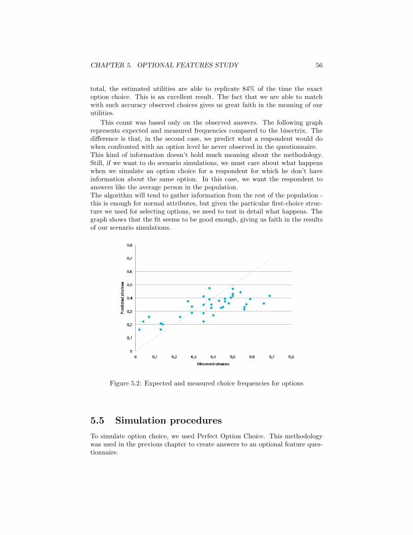
CHAPTER 5. OPTIONAL FEATURES STUDY 56
total, the estimated utilities are able to replicate 84% of the time the exactoption choice. This is an excellent result. The fact that we are able to matchwith such accuracy observed choices gives us great faith in the meaning of ourutilities.
This count was based only on the observed answers. The following graphrepresents expected and measured frequencies compared to the bisectrix. Thedifference is that, in the second case, we predict what a respondent would dowhen confronted with an option level he never observed in the questionnaire.This kind of information doesn’t hold much meaning about the methodology.Still, if we want to do scenario simulations, we must care about what happenswhen we simulate an option choice for a respondent for which he don’t haveinformation about the same option. In this case, we want the respondent toanswers like the average person in the population.The algorithm will tend to gather information from the rest of the population -this is enough for normal attributes, but given the particular first-choice struc-ture we used for selecting options, we need to test in detail what happens. Thegraph shows that the fit seems to be good enough, giving us faith in the resultsof our scenario simulations.
Figure 5.2: Expected and measured choice frequencies for options
5.5 Simulation procedures
To simulate option choice, we used Perfect Option Choice. This methodologywas used in the previous chapter to create answers to an optional feature ques-tionnaire.

CHAPTER 5. OPTIONAL FEATURES STUDY 57
In Perfect Option Choice, an option is chosen with probability one when theutility of choosing it is higher than for not choosing it.
We have a reason to use this method. Observing the data, we were ableto see that respondents were very consistent in their choices of options. If anoption was selected at a certain price in one question, it is extremely likely itwould be selected again at the same price in the following questions.We assume that this stems from the particular structure of options: they areinherently simple objects.An option is made by an attribute and a price. For a person that knows themarket, it is very easy to tell if an option is cheap or not, expensive or not.Therefore, evaluation of options tend to be consistent, and selections tend to beconsistent.Of course, there may be cases when this consistency is not present. We thinkthat this can be explained by other reasons, for example by budget constraintslogics. If there is a maximum amount of money a person can spend, the selectionof an option depends not only on its intrinsic value, but also on the amount thatis spent for the core products and the other options. Generally it is consideredthat, when budget constraints are present, the options with the higher utilityper amount of money are selected first.
5.5.1 Improvement over old estimation procedure
First and foremost, the new methodology produces utilities that really matchthe choices made by respondents. All the information provided by the respon-dents when answering the questionnaire is taken into consideration and can beretrieved from the coding in the model.
Adding the Not Chosen level it is now possible to forecast choice of optionsin scenario simulations.This is a major improvement: it is a utilities-based way to forecast the choiceof options.With this knowledge it is now possible to perform precise forecasts.
It is now possible to know if options add complexity to the product. If theutility for Not Chosen is higher than Not Present, offering the product makesthe product complicated. In simple terms, this is like saying that people arehappier when they are not offered the option than when they see it (and decidenot to buy it).It is arguable if this interpretation of the results makes sense for all respondents.Does offering an option that I decide to buy increase the complexity of theproduct? Should we do this analysis only for people that did not/would notselect the option?In a certain sense, it is more prudent to do so. In a deeper sense, adding alot of very interesting options that most customers will buy makes the productnonetheless more complicated. It does take more time to analyze it, even thoughthe total complexity effect may be diminished by the fact that respondent likethe options. What we suggest to do is, for products with a limited number of
CHAPTER 5. OPTIONAL FEATURES STUDY 58
options to consider the difference between Not Chosen/Not Present for a givenoption only for people that would not select that option.
With this methodology it is possible to study the halo effect. If, for a givenoption, the utility for Not Chosen is higher than for Not Present, it means thatpeople are happier when they see the option (regardless if they are going to buyit or not) than when they don’t see it. The interpretation for the halo effect issimpler than for the complexity effect. We can think that the halo effect doesnot depend on the option selection. It is probably even stronger for the peoplethat are buying the option.
In conclusion, with the new methodology a whole new range of businessquestions can be answered.Now it is possible to analyze the effect each option has on the global evaluationof the product. This is extremely important in analyzing a scenario. We are ableto tell if offering an option will move customers from one product to another.This can happen in two ways: the option may be increase interest for customers,or drive them away by making the product too complex. This information isextremely important when taking strategic decisions.

Chapter 6
Bundles
Bundles are defined as a collection of features or services that are offered to-gether, for a single price, as an addition to some product or service.They are closely related to optional features and have similar advantages anddisadvantages but their structure is much more complex to analyze.
From the point of view of the consumer, the existence of bundles is importantfor two characteristics:
• convenience: when a consumer has to analyze complex offering of productsthat are meant to work together (es. Selecting a fully comprehensive finan-cial service that covers funding, pension, insurance etc), an offer featuringa sensible combination of many products provides a solution. A consumerwith limited expertise in the market may be interested in making a singlechoice instead of many difficult one.
• discount: it is very common for the bundle features to be also sold on theirown. Usually when buying a bundle of features the price of the bundle islower than the total price of the features considered singularly. A customerinterested only in some features may buy a bundle containing other notso interesting features if the total price is low enough. This behavior iswell established in the experimental literature.
From the seller’s point of view, the reason for offering bundles is mainly toincrease the out of pocket expense. When a must-have feature is only offered ina bundle, the customer is forced to buy the whole bundle, paying for featuresthat may be uninteresting for him/her.This may not be seen as unfair by the customer - there is evidence in literature([11], [2]) that customers accept as fair a bundle with some uninteresting featuresas long as all the components in the bundle ”make sense” when consideredtogether.For example, in a house insurance product, a service bundle containing extrainsurance for flooding, fire and structural failure may be considered fair as thethree features are pertaining to the same area.

CHAPTER 6. BUNDLES 60
When features are offered in bundles or on their own, a customer may want tobuy a bundle even if it contains uninteresting features, as long as the total priceis low enough. Therefore, offering a bundle increases the total out of pocketcost.This behavior is well known and it has been observed many times.
6.1 the Bundle study
SKIM was much interested in finding a way to analyze bundles in a CBC context.It was decided to test methodologies based on optional features on simulateddatasets and, if the results looked promising, test them on real data.Tests were run on simulated datasets and the results looked good. We thereforedecided to try them on real data. The company had no datasets about bundlesarising from previous studies, so it was decided to organize a field study just totest these methodologies.
The description of this study and the estimation results are found in thenext chapter. In this chapter we’ll describe assumptions and considerationsthat draw our analysis.
6.2 Differences and similarities with optional fea-tures
In our classification, we divide all bundles in two possible types.
We can discriminate between bundles that offer services that can be substi-tuted or not. In the first case, one could buy a product without the bundle andobtain in a second moment products equivalent to the one of the bundle. Theprovider in this second purchase could be the same or a different company fromwhich he/she bought the product: in this case we are speaking about (delayed)upgrades.When a service can be bought only from the provider of the core product andonly at the moment of purchase, the seller has considerable power when thebundle has some ”must have” features.
We limit our investigations to bundles that can only be provided by thecompany providing the core product. This makes the analysis much easier.
We will not consider in detail the case of delayed upgrades. We will notinvestigate the likeliness of upgrading at a second stage. We only want to knowwhich bundles are going to be selected at the moment of purchase of the coreproduct.
Our main assumption about bundles is that there is such a thing as a bundleprice elasticity. This means that it is possible to study the price elasticity ofa bundle without knowing what items it has. This is clearly an oversimplifica-tion: two bundles with the same price and different items clearly have different
CHAPTER 6. BUNDLES 61
elasticities.This is especially evident if one thinks of the case of single-item bundles.
Still, this simplification works pretty well with bundles made of many items.Also, from a purely practical point of view, studying the bundle price elasticityas depending on the bundle content would mean finding a way to divide thetotal price among bundle components. This would of course give better results.Still, it would be very complicated. It is our opinion is that it is not possible touse such an approach using only the information gathered from a conjoint-stylestudy.
6.2.1 Interaction effect
In many real life examples bundles are often rather expensive compared to thecore product and can constitute a significant fraction of the total price.Therefore, the interaction between core price and bundle price can be verystrong. We did not study in detail this interaction when modeling options sincewe decided to consider only options whose price was little compared to the coreproduct price.If budget constraints behavior happen in the choice of options, they are easilycaptured in the heterogeneity of the model. Also, offering many options forlimited prices, it is easy to see if psychologic threshold are present. If customerare for example shy of spending more than 100 euro but they have enoughoptions to arrive close to that amount it is quite easy to detect this thresholdas many will buy options for a total just under 100 and other will buy optionfor a total well over 100, leaving a space between 100 and, say 120, with littleobserved choices.When studying bundles it is harder to detect such behavior, since bundles mayconstitute a huge part of the total price.
When designing the bundle study, we decided to study a class of productsthat had a strong interaction between bundle and core price.Our choice was the market of credit cards.
6.2.2 Goals of the model
The goal of our bundle model is to provide utilities on a respondent level.The data used to estimate utilities must only come from realistic choice tasks.These utilities describe core products and bundles and reproduce the observedanswers. By this we mean that only knowing the utilities we would be able toanswer the questionnaire in a way similar to the one of the respondents.
6.2.3 Limitations of the model
As we will describe in detail in the next chapter, we studied the problem ofbundles when a single bundle is offered with each product.In reality, the situation can be much more complex. For example, with a single
CHAPTER 6. BUNDLES 62
core product many extras may be offered at once. For example, one might havemany optional features and bundles made of some of those optional features.Our simple model is not meant to analyze such a situation. One could use it toanalyze complex situations - after all, knowing utilities one can simulate choicesof any combination of bundles and options. Still, we advise not to take theanalysis too far: given a complex situation, with many interrelated bundles andoptions, unknown dynamics might be present in the choice procedure.
6.3 Utility from a business perspective
As we will show in the next chapter, we were able to create a working method-ology for bundles.From a business point of view, a bundle methodology leads to great answers.The result of the estimation is a set of utilities for each respondent.With this utility we can simulate the respondent’s behavior in various scenarios.That is, we can perform realistic simulation.
We therefore can make prediction on the number of people that will select acertain bundle, we can assess market shares, income forecasts and cannibaliza-tion risks.
Also, these results can be used in product definition: we can find the optimalbundle for a certain objective (es increasing market share, increasing revenuesetc).
Chapter 7
Results of the Bundlesstudy
Results of the Bundle study
7.0.1 Characteristics of the study
The Bundle study is a study devised to test new methodologies. The goal is tofind a way to handle bundle data arising from conjoint-style choice exercises.This study was funded and managed by SKIM Analytical and its results arepublished by kind permission.The topic of the study is credit cards.
The study was directed to Dutch respondents. It was administered via in-ternet until a total of 250 completed entries was reached.Data was collected from the 23th to the 28th of July 2009.
The questionnaire started with questions about how credit card are used:how often, to buy what and how much their yearly fee is.Then the respondents were requested to perform 12 choice tasks, similar to theones used in conjoint studies. They only difference is that for each productshown on screen it was possible to select a bundle of services for an extra price.The questionnaire finished with more questions about demographical detailsand likeliness of choosing a new credit card in the next future.
There was no particular screening to select the population of respondents.People of all ages were invited to take part in the questionnaire. However, theiranswers to some questions could stop them from completing the questionnaire.Most notably, people who had a credit card but used it too few times in a yearwere screened out as considered not interesting for the questionnaire.

CHAPTER 7. RESULTS OF THE BUNDLES STUDY 64
Structure of the questionnaire
1. How old are you?1. Less than 18 years old - disqualified2. 18-29 years old3. 30-39 years old4. 40-49 years old5. 50-64 years old6. 65+ years old -disqualified
2. Do you have a credit card?1. Yes, one that is my own and one from my employer2. Yes, only from my employer3. Yes, only my own4. No, I don’t have a credit card
3. What is the brand of your credit card? If you have more thanone, choose the one you use more oftenPictures of 34 credit cards from ABN AMRO, American Express, ANWB, Fortis,ING, Postbank, Rabobank, SNS, Visa appear.
4. How often do you use your credit card?1. Once per year or less - disqualified2. Once every three months3. At least once per month4. Each week5. Many times a week6. Each day
5. Who in your household decides to purchase or to modify thecontract (cancel, renew, change, etc.) of your credit card?1. Me2. My partner - disqualified3. Me and my partner
6.Do you have more than one (personal) credit card?1. Yes2. No
7. From what bank or institution is your private credit card?Reporting the selection in question 3
8. Do you know what is the yearly fee of your personal, most usedcredit card?1. Yes, it is Euro ... per year

CHAPTER 7. RESULTS OF THE BUNDLES STUDY 65
2. No
8b. If not, what range is it in?1. From 0 to 5 Euro per year2. From 5 to 15 Euro per year3. From 15 to 25 Euro per year4. From 25 to 35 Euro per year5. From 35 to 45 Euro per year6. From 45 to 55 Euro per year7. More than 55 Euro per year8. I don’t know
9. What do you use your credit card for? Multiple answers possi-ble.1. Buying gas2. Booking holidays (either by travel agency or by internet)3. Buying on the internet (no holidays)4. Groceries shopping (total cost of less than 100 Euro)5. Groceries shopping (total cost of more than 100 Euro)6. Going out7. Other activities, namely
10. Divide in percentage all your credit card purchases among thefollowing categories:List of answers chosen in the previous question
11. Please specify the percentages of your transactions takingplace in the Netherlands and in foreign countries
12. How likely are you to change your credit card in the next twoyears?Very likelyLikelyA bit likelyI don’t knowA bit unlikelyUnlikelyVery unlikely
12b. If unlikely: what is the main reason you find it unlikely tohappen?
12c. If likely: what is the most important reason you find it likelyto happen?

CHAPTER 7. RESULTS OF THE BUNDLES STUDY 66
13. Please indicate how much do you agree with each of the fol-lowing statementsA list of statements appears. For each statement it is possible to select oneamong: Totally agree, Agree In part, Don’t agree nor disagree, Disagree in part,Disagree, No opinion
The statements are:Each credit card brings with it a bit of insecurityWith a credit card I never need to worry that I don’t have moneyWith a credit card I find myself in debt easierMy credit card provider to protect me protection against building of a big debtA credit card gives me statusA credit card is practicalI’m afraid that somebody could commit a fraud with my credit cardA credit card gives me services that not everyone has
14. Choice tasksTwelve choice tasks, each featuring 4 products, each one with one bundle, anda None of the above/No choice option.
15. What is your sex?1. Male2. Female
16. Which of the following better describes you?1. Living with my family2. Living on my own3. Married/living with my partner4. Student house/residential community5. Other, namely
17. How many children are there in your house?
18. What is your income range?1. Less than 20.000 Euro/year2. Between 20.000 and 30.000 Euro/year3. Between 30.000 and 40.000 Euro/year4. Between 40.000 and 50.000 Euro/year5. Between 50.000 and 60.000 Euro/year6. Between 60.000 and 70.000 Euro/year7. Between 70.000 and 80.000 Euro/year8. More than 80.000 Euro/year9. I prefer not to answer this question

CHAPTER 7. RESULTS OF THE BUNDLES STUDY 67
19. What is your higher level of education? 1. Lagere school / none2. MAVO / MULO / lager beroepsonderwijs3. HAVO / VWO / HBS4. Middelbaar beroepsonderwijs5. Hoger beroepsonderwijs6. University
20 Which of the following options better describes your workingsituation?1. Full-time employed worker2. Part-time employed worker3. Full time independent worker4. Part-time independent worker5. I am a housewife/househusband6. I don’t work7. I am a student8. I am retired9. No answer
21. What are the four cyphers of your postcodes?
7.0.2 Choice task design
For each respondent 12 questions were generated. Each question featured 4products, each coming with a bundle.The respondent could choose one of the 4 products or select a No Choice option.This picture shows the choice task structure:

CHAPTER 7. RESULTS OF THE BUNDLES STUDY 68
7.0.3 Attributes
The core product was defined by the following attributes and levels:
• Brand: ING Rabobank, SNS Bank,, ABN AMRO, Fortis, VISA, Master-card, American Express
• Price: Euro 10, Euro 15 , Euro 20, Euro 25, Euro 30, Euro 35, Euro 40,Euro 45, Euro 50, Euro 60, Euro 70
• Effective interest: 8% per year, 10% per year, 12% per year, 14% peryear, 16% per year
• Limit on CC: Euro 500 Euro 1.500, Euro 2.500, Euro 5.000, Euro 10.000,Euro 20.000
• Purchase insurance: Not present, 100 days, 200 days, 1 year
The bundles were defined by the following attribute and levels:
• Additional purchase insurance: 100 extra days, 200 extra days, Notpresent
• Additional travel insurance: Present, Not present
• Travel inconvenience insurance: Present, Not present
• Credit protection insurance: Present, Not present
• SMS alert: Present, Not present
• Statement fee: Present, Not present
Level balance
The questionnaire was generated in two separate moments.First, the part relative to core products and then the part relative to bundleswas generated.Core products were generated automatically by using Sawtooth SSI Web soft-ware. A balanced design (showing levels of an attribute with equal frequency)was chosen.
A similar feat was obtained for bundle levels.We decided to study bundles with one to four items.On a global level, we wanted bundles to have this distribution: 20% one item,30% two items, 30% three items and 20% four items.Therefore the coding is not perpendicular: the Not Present level will be seenmore often.

CHAPTER 7. RESULTS OF THE BUNDLES STUDY 69
We also wanted to achieve balance on a respondent’s level.On the 48 bundles each respondent sees (4 bundles for each of the 12 questions),we want the global percentages to be observed. Therefore we decided to allocatefor each respondent 10 bundles with one and three items and 14 bundles withtwo and four.We also wanted balance on a respondent level, i.e. we want each respondent tosee a given level the same number of time.This is the way we created the bundles for each respondent.First we allocated for each respondent a number of levels values from which todraw.For example, for Attribute 1, we can draw level Not Present 28 times and Present20 times. The distribution is such that, for each respondent, it is possible toarrange in some way the levels to form 10 bundles with 1 feature, 14 with twoetc.We create bundles randomly sampling without replacements from this distribu-tion.We sample a level from each attribute and consider the resulting bundle. Thenwe see if the bundle is not suitable: for example, if it has 6 items, or if it has 3and we already created all 3-items bundles for that respondent.If this is the case, we ”put back” the drawn levels and draw another bundle. Ifwe have to repeat a draw more than a certain number of times, we conclude weare in a dead end and start all over again for that respondent.
This is not the optimal way to create a questionnaire but it is very fast. TheVB code to generate the questionnaire is contained in the bundle gen.xls file.
Bundles generated with the VB code and core products generated by SSIWeb were mixed randomly to create questions. From a practical point of view,this means that expensive bundles can be offered with cheap credit cards andviceversa.
Discount structure
The price of bundles was calculated on the following way.For each item present in the bundle, a price was generated. The price for eachitem is random from a list of values. These values are:
• Additional purchase insurance: 1 Euro, 2,5 Euro, 5 Euro
• Additional travel insurance: 1 Euro, 2,5 Euro, 5 Euro
• Travel inconvenience insurance: 2,5 Euro, 5 Euro, 7,5 Euro
• Credit protection insurance: 2,5 Euro, 5 Euro, 7,5 Euro
• SMS alert: 1 Euro, 2,5 Euro, 5 Euro
• Statement fee: 2,5 Euro, 5 Euro, 7,5 Euro

CHAPTER 7. RESULTS OF THE BUNDLES STUDY 70
The price of the bundle is then the sum of the singular items price, with adiscount. If the bundle has two items, the discount is 10 % , if it has three thediscount is 20 % and it is 30 % when there are four items.
A discount structure is very realistic feature, since bundles usually have alower total price than single goods. This is of course to stimulate a higherout-of-pocket expense.
Total price
During the design phase it was a matter of discussion wether respondents shouldsee on screen the total price (core+bundle) when they decide to select a bundle.It was decided that this price should not be shown automatically on screen.
Showing it would probably enforce a stronger interaction between core priceand bundle price and it wouldn’t add realism to the questionnaire.
Filtering
The only post-hoc filtering of respondents was based on their answering time.The average time to answer the whole questionnaire was estimated as 15 min-utes. Respondents finishing the questionnaire in less than 5 minutes were takenout of the sample.This resulted in a sample of 205 respondents from the original 250.
7.0.4 The choice tasks
After the filtering, a bundle was selected in 194 choice tasks out of 1709 (11,35% ). This percentage is calculated only considering the questions whose answerwas different from the None/no choice answer.Only 49 respondents out of 205 selected a bundle at least once.
The No choice answer was selected 751 times out of the 2460 questions (12questions * 205 respondents), resulting in a percentage of 30,5 % .This is a pretty high percentage. The number of No choice selections is notincreasing question after question (from question 1 to 12: 52 60 61 60 65 63 6863 64 69 59 67).This makes us think that these answers are to be taken as serious.Probably respondents had a very precise idea of what kind of card they lookfor and they are not ready to settle for something else. We studied a ratherlarge range of prices for credit cards (from 10 Euro to 35 Euro yearly fee) so itis more probable for one respondent not to have a card in his/her favorite pricerange among the 4 on screen.
We tried to see if bundles were selected more often by a certain class ofrespondents. In particular, we wanted to know if there was a link between thecurrent yearly expenditures and bundle selection.

CHAPTER 7. RESULTS OF THE BUNDLES STUDY 71
Table 7.1: Distribution of respondents selecting at least one bundle
expenditure range respondents thatselected bundles
number of respon-dents in class5cm
percentage
0-5 euro/year 3 15 20,00%5-15 euro/year 6 30 20,00%
15-25 euro/year 11 44 25,00%25-35 euro/year 8 27 29,63%35-45 euro/year 5 18 27,78%45-55 euro/year 4 9 44,44%
more than 55 euro/year 1 8 12,50%don’t knot/don’t say 11 53 20,75%
49
What we can see from the table is that even respondents in the low payingrange selected bundles.It seems that bundle selection gets slightly more frequent as yearly fee rises.This increase is interesting, but the discovery that also low and middle rangespenders select bundles has far more important commercial consequences.
Coding for the CBC-HB estimation
To run the CBC-HB algorithm on the data, the bundles were coded in thefollowing way:
• If a bundle was selected, the attributes of the bundles of all products inthe choice task are left untouched. An extra product is added. Its coreproduct levels are the same of the chosen product. All its bundles levelsare coded as Not Present, and it’s price is coded as 0, meaning it doesn’thave an utility that is taken into considerations in the algorithm.
• If no bundle was selected, the bundle is coded with the new value “Notpresent” for all the products in the choice task. The bundle price for allproducts is 0, meaning that an utility of 0 is used in the iteration. Anextra product is added. This product is equal to the chosen product butits bundle has the original attribute values of the chosen product, priceincluded.
a picture will make it clearer.The coding is therefore:
This coding is different from the coding used for options for two main reasons:
• Price: the price of non-chosen options was used as data in the estimation,the price of non-chosen bundles is not

CHAPTER 7. RESULTS OF THE BUNDLES STUDY 72
Table 7.2: Answer of a bundle choice task (chosen bundle)
Product 1 Product 2 Product 3 Product 4
Core Attribute 1 A1 A2 A1 A2Core Attribute 2 B1 B2 B2 B1
Core Price (Euro) 10 15 12 20Bundle attribute 1 Present Not Present Present Not PresentBundle attribute 2 Not Present Present Present Present
Bundle Price (Euro) 4 5 3 4Chosen Y/N X
Choice •
Table 7.3: Coding (chosen bundle)
Product 1 Product 2 Product 3 Product 4 Product 5
Core Attribute 1 1 2 1 2 2Core Attribute 2 1 2 2 1 2
Core Price (Euro) 1 3 2 4 2Bundle attribute 1 1 2 1 2 2Bundle attribute 2 2 1 1 1 2
Bundle Price (Euro) 2 3 1 2 0Choice •
Table 7.4: Answer of a bundle choice task (bundle not chosen)
Product 1 Product 2 Product 3 Product 4
Core Attribute 1 A1 A2 A1 A2Core Attribute 2 B1 B2 B2 B1
Core Price (Euro) 10 15 12 20Bundle attribute 1 Present Not Present Present Not PresentBundle attribute 2 Not Present Present Present Present
Bundle Price (Euro) 4 5 3 4Chosen Y/N ×
Choice •
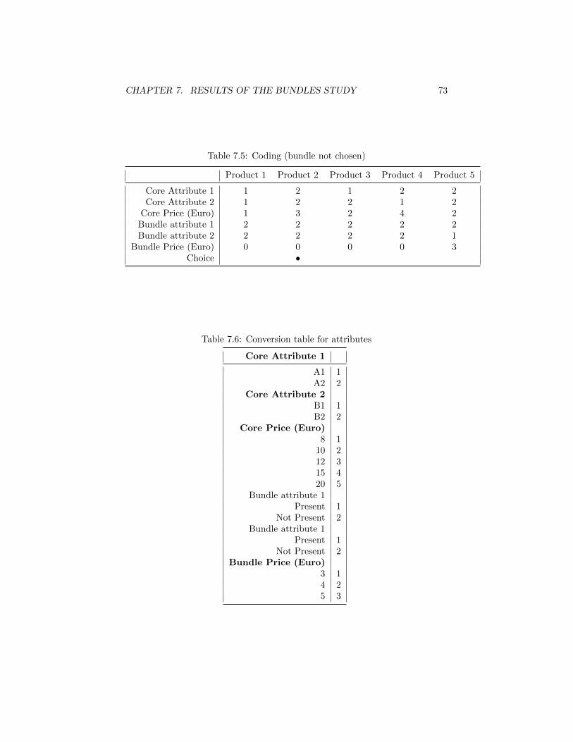
CHAPTER 7. RESULTS OF THE BUNDLES STUDY 73
Table 7.5: Coding (bundle not chosen)
Product 1 Product 2 Product 3 Product 4 Product 5
Core Attribute 1 1 2 1 2 2Core Attribute 2 1 2 2 1 2
Core Price (Euro) 1 3 2 4 2Bundle attribute 1 2 2 2 2 2Bundle attribute 2 2 2 2 2 1
Bundle Price (Euro) 0 0 0 0 3Choice •
Table 7.6: Conversion table for attributes
Core Attribute 1
A1 1A2 2
Core Attribute 2B1 1B2 2
Core Price (Euro)8 1
10 212 315 420 5
Bundle attribute 1Present 1
Not Present 2Bundle attribute 1
Present 1Not Present 2
Bundle Price (Euro)3 14 25 3

CHAPTER 7. RESULTS OF THE BUNDLES STUDY 74
• Not Present & Not Chosen: for options there was a difference when anoption was shown but not selected or when it was not selected at all. Forbundles only the Not Present level is used.
This coding was developed basing on the ones used for options, with NotPresent and Not Chosen levels, but the prediction rate was low.Also, for respondents that selected many bundles, the two levels tended to havesimilar values.Other codings we tried, and at the end the best results were obtained by over-riding the Not Chosen attribute with Not Present.
7.0.5 Results
With this coding we are able to predict 69, 38% of the bundles. This is an excel-lent result, meaning the prediction rate is good enough to be used in practice.This percentage only refers to bundle prediction: given the utility and the bun-dle features alone, the number of time the predicted bundle choice is the sameas the observed one.For the alternatives prediction rate (that is, prediction of which of the fourproduct will be chosen) the result is equally good with a rate of over 70%.These results were obtained with constraints on the price (utility of lower prices> utility of higher prices).
Table 7.7: Prediction rates
Observed selections Predicted selections
Question 1 20 10Question 2 21 11Question 3 25 17Question 4 21 12Question 5 19 9Question 6 19 9Question 7 18 6Question 8 17 11Question 9 14 5
Question 10 13 7Question 11 18 7Question 12 13 4
Looking at the prediction rate it is possible to see where it is possible toimprove. The distribution clearly underestimate bundle selections.Looking at the single predictions as reported in bundle results.xlsm, sheet bundlecounter 2, it is possible to see that the algorithm creates both false positivesand false negatives. This is a good feature, meaning that the algorithm doesn’t

CHAPTER 7. RESULTS OF THE BUNDLES STUDY 75
”need” an overwhelming amount of recorded choices to decide to predict a bun-dle selection. This was actually the problem with the first, optional features-likecoding.
7.0.6 Comment on the coding
The coding of bundles is not just a trick to improve estimation, it has someimportant consequences.
Its differences from the optional features coding tell us a lot about the waybundles work.For example, the Not Chosen level is not present anymore in this coding. Thislevel was used for optional features to indicate an option that was offered andnot chosen, while Not Present indicated an option that was not featured andcould not be chosen.For bundles, the two are the same. For options, the difference in utility betweenNot Chosen and Not Present meant that some options added value to the coreproduct even when not selected. In many cases, using the same coding forbundles, the difference between the two values was very low and the predictionrate was not satisfactory.Even if the two parameters are, in a certain way, the same, writing it as twomakes the design less orthogonal and therefore the estimation not as precise.This difference means that bundles are considered as one and, if not selected,their presence has no influence on the evaluation of the core product.
Speaking of prices, for options the price of an unselected option was takenin consideration much more heavily.If an option was selected for a certain product, the prices of the same optionsin other products were included in the coding.Also, when an option was not selected it was recorded the price at which it wasnot chosen. In our interpretation, this meant that the price at which an optionwas offered was important. The information was processed and kept in mindby the respondent.For each option the price was a part of the levels: for example for option Apossible levels would be: Not Present, Not Chosen, Present at 1 Euro, Presentat 2 Euro etc.This gave us the possibility to measure the price sensitivity for each option.
Now, for bundles, the situation is different. It is not possible to define pricesensitivity for single bundle items if we don’t know how respondents allocatethe total bundle price between items.Therefore, it is only possible to measure price sensitivity for the whole bundle.This could be due to the fact that bundles are inherently more complex thanoptions.People processes their decision on a bundle and then discard the data, whilethe price of options - simpler objects- lingers on in the respondent’s mind. Thiscauses an halo effect.
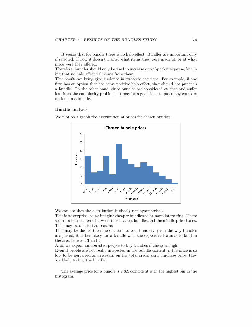
CHAPTER 7. RESULTS OF THE BUNDLES STUDY 76
It seems that for bundle there is no halo effect. Bundles are important onlyif selected. If not, it doesn’t matter what items they were made of, or at whatprice were they offered.Therefore, bundles should only be used to increase out-of-pocket expense, know-ing that no halo effect will come from them.This result can bring give guidance in strategic decisions. For example, if onefirm has an option that has some positive halo effect, they should not put it ina bundle. On the other hand, since bundles are considered at once and sufferless from the complexity problems, it may be a good idea to put many complexoptions in a bundle.
Bundle analysis
We plot on a graph the distribution of prices for chosen bundles:
We can see that the distribution is clearly non-symmetrical.This is no surprise, as we imagine cheaper bundles to be more interesting. Thereseems to be a decrease between the cheapest bundles and the middle priced ones.This may be due to two reasons.This may be due to the inherent structure of bundles: given the way bundlesare priced, it is less likely for a bundle with the expensive features to land inthe area between 3 and 5.Also, we expect uninterested people to buy bundles if cheap enough.Even if people are not really interested in the bundle content, if the price is solow to be perceived as irrelevant on the total credit card purchase price, theyare likely to buy the bundle.
The average price for a bundle is 7.82, coincident with the highest bin in thehistogram.
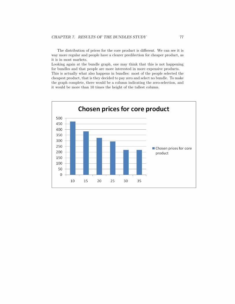
CHAPTER 7. RESULTS OF THE BUNDLES STUDY 77
The distribution of prices for the core product is different. We can see it isway more regular and people have a clearer predilection for cheaper product, asit is in most markets.Looking again at the bundle graph, one may think that this is not happeningfor bundles and that people are more interested in more expensive products.This is actually what also happens in bundles: most of the people selected thecheapest product, that is they decided to pay zero and select no bundle. To makethe graph complete, there would be a column indicating the zero-selection, andit would be more than 10 times the height of the tallest column.
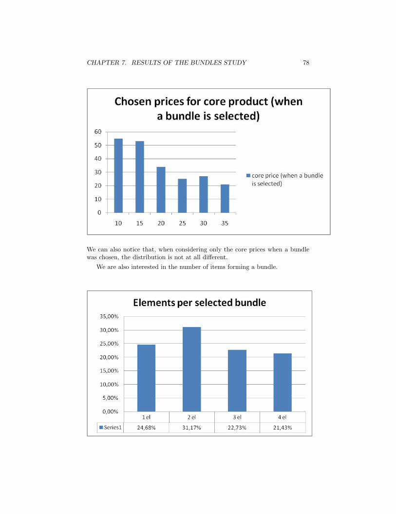
CHAPTER 7. RESULTS OF THE BUNDLES STUDY 78
We can also notice that, when considering only the core prices when a bundlewas chosen, the distribution is not at all different.
We are also interested in the number of items forming a bundle.
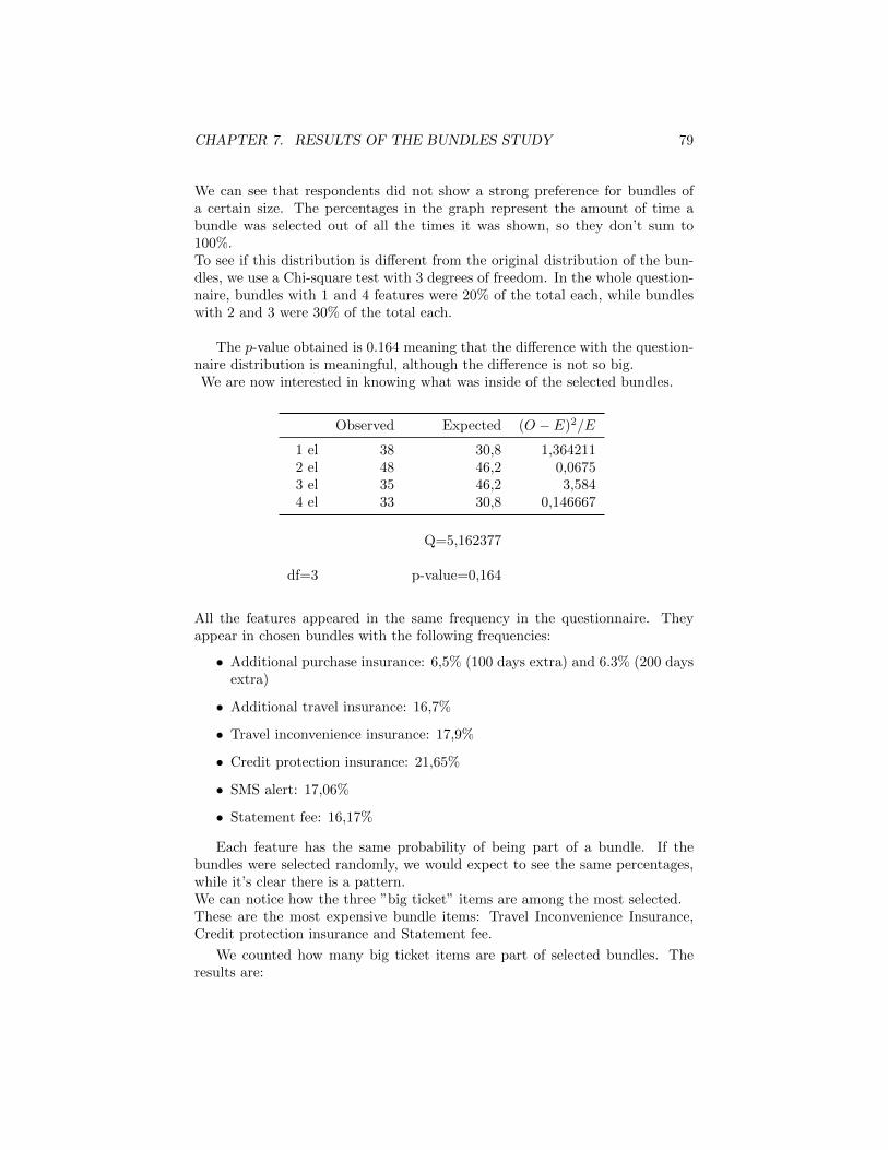
CHAPTER 7. RESULTS OF THE BUNDLES STUDY 79
We can see that respondents did not show a strong preference for bundles ofa certain size. The percentages in the graph represent the amount of time abundle was selected out of all the times it was shown, so they don’t sum to100%.To see if this distribution is different from the original distribution of the bun-dles, we use a Chi-square test with 3 degrees of freedom. In the whole question-naire, bundles with 1 and 4 features were 20% of the total each, while bundleswith 2 and 3 were 30% of the total each.
The p-value obtained is 0.164 meaning that the difference with the question-naire distribution is meaningful, although the difference is not so big.We are now interested in knowing what was inside of the selected bundles.
Observed Expected (O − E)2/E
1 el 38 30,8 1,3642112 el 48 46,2 0,06753 el 35 46,2 3,5844 el 33 30,8 0,146667
Q=5,162377
df=3 p-value=0,164
All the features appeared in the same frequency in the questionnaire. Theyappear in chosen bundles with the following frequencies:
• Additional purchase insurance: 6,5% (100 days extra) and 6.3% (200 daysextra)
• Additional travel insurance: 16,7%
• Travel inconvenience insurance: 17,9%
• Credit protection insurance: 21,65%
• SMS alert: 17,06%
• Statement fee: 16,17%
Each feature has the same probability of being part of a bundle. If thebundles were selected randomly, we would expect to see the same percentages,while it’s clear there is a pattern.We can notice how the three ”big ticket” items are among the most selected.These are the most expensive bundle items: Travel Inconvenience Insurance,Credit protection insurance and Statement fee.
We counted how many big ticket items are part of selected bundles. Theresults are:

CHAPTER 7. RESULTS OF THE BUNDLES STUDY 80
• No big ticket item: 22,44
• One big ticket item: 41,67
• Two big ticket item: 32,29
• Three big ticket item: 3,21
• Four big ticket item: 0
Most bundles have just one or two elements. We will use this information tocreate the optimal configuration for a bundle.
We are also interested in studying the interaction between the ”Purchase in-surance” attribute of the core product and the ”Additional purchase insurance”present in the bundles.In the questionnaire, bundles with additional purchase insurance were not pro-posed with cards that had no purchase insurance.The results were the following:
Table 7.8: Link exra insurance-insurance in core product
extra purchase in-surace in selectedbundle
not present 100 days 200 days 1 year total
not present 44 31 37 45 113100 extra 0 11 11 11 33200 extra 0 12 6 10 28total 54 54 66 174
We were therefore interested in studying the link between the two. We testedindependence between the two factors with a Chi-square test. The p-value is0.55 meaning that the two factors are not independent.
100 days 200 days 1 year
not present 35,06897 35,06897 42,86207100 extra 10,24138 10,24138 12,51724200 extra 8,689655 8,689655 10,62069
We also studied the price sensitivity for bundles. The biggest decreases isbetween 4 and 5. Another smaller decrease happens before 10. We can regard5 and 10 as psychological price barriers.

CHAPTER 7. RESULTS OF THE BUNDLES STUDY 81
100 days 200 days 1 year
not present 0,472112 0,10633 0,106639100 extra 0,056194 0,056194 0,183908200 extra 1,261084 0,832512 0,036274
Q=3,1112473236367p-value=0,211
Optimal configuration
With the insight gained with our analysis, we cam calculate the optimal config-uration for a bundle offer.This configuration is based on utilities and the analysis we carried on earlier.First we have to decide how many bundles to offer. In the questionnaire westudied only one bundle per product, but we can use utilities to see what wouldhappen when more bundles are offered.It is possible to simulate bundle choices in the sheet utils of bundle results.xlsm.
After trying various combinations, our proposal is the following: two bun-dles, a cheap one and a middle-priced one, with no elements in common.The best structure for this configuration is:

CHAPTER 7. RESULTS OF THE BUNDLES STUDY 82
Bundle 1: travel protection insurance, credit protection insurance, SMS alertfor 9.50 EuroBundle 2: statement fee for 4 Euro.
With this configuration, a total of 32 respondents (out of 49) would selectat least one bundle.Twenty-three would select the first bundle, twenty one would select the second.This mean that twelve respondents would select both of them.From our point of view, since one bundle is quite cheap compared to the other,we can expect many people to select both of them. These two bundles containall items a part from Additional Purchase Insurance, the least selected item inthe study.
Chapter 8
CBC HB estimationalgorithm in R
The algorithm presented in this chapter replicates the one implemented by Saw-tooth Software CBC-HB.It was decided to implement this algorithm in the open source language R sothat everybody could replicate the results shown in this thesis without the needto pay for proprietary software.This algorithm has its own way to code the input files but we wrote a VB codeto pass from Sawtooth input format to R input format.The code is partly based on the R package bayesm, written by Rossi E., AllenbyG., McCulloch R., and freely available to download and modify under the GPLlicence.The package for bayesm is available at the site http://cran.r-project.org/
web/packages/bayesm/index.html.
Our implementation of the CBC HB algorithm with a test example is con-tained in the archive attached to the thesis.
8.1 Running the program
To illustrate how to use the program, we consider a test run.
In this example 300 respondents partecipated in a survey.Each respondent answered 12 choice tasks, each one with 5 alternatives.Products were defined by four attributes, each one having seven levels, num-bered 1 to 7.

CHAPTER 8. CBC HB ESTIMATION ALGORITHM IN R 84
8.1.1 Design matrix and answers
The design matrix is recorded in the object lgtdata, a list with a number ofentries equal to the respondents number.One entry, the one for respondent number 300, looks like this:
>lgtdata[[300]]
$y
[1] 4 2 4 1 1 3 1 4 4 2 3 3
$X
[,1] [,2] [,3] [,4] [,5] [,6] [,7] [,8] [,9] [,10] [,11] [,12] [,13]
[1,] 0 0 0 0 0 1 0 0 0 0 0 1 1
[2,] 0 0 0 0 0 1 0 0 0 0 0 1 0
[3,] 0 0 0 0 0 1 0 0 0 0 0 1 0
[4,] 0 0 0 0 0 1 0 0 0 0 0 1 0
[5,] 0 0 0 0 0 0 0 0 0 0 0 0 0
....
[55,] 0 0 1 0 0 0 0 0 0 0 0 1 0
[56,] 0 0 0 0 0 1 0 0 1 0 0 0 0
[57,] 0 0 0 0 0 1 0 1 0 0 0 0 1
[58,] 0 0 0 0 0 1 1 0 0 0 0 0 0
[59,] 0 0 0 0 0 1 0 0 0 0 1 0 0
[60,] 0 0 0 0 0 0 0 0 0 0 0 1 0
[,14] [,15] [,16] [,17] [,18] [,19] [,20] [,21] [,22] [,23] [,24]
[1,] 0 0 0 0 0 0 0 0 0 0 1
[2,] 0 1 0 0 0 0 0 0 0 0 1
[3,] 0 0 1 0 0 0 0 0 0 0 1
[4,] 0 0 0 1 0 0 0 0 0 0 1
[5,] 0 0 0 0 1 1 0 0 0 0 0
....
[55,] 0 1 0 0 0 1 0 0 0 0 0
[56,] 0 0 0 1 0 0 0 0 0 0 1
[57,] 0 0 0 0 0 0 0 0 0 0 1
[58,] 0 0 0 0 0 0 0 0 0 0 1
[59,] 0 1 0 0 0 0 0 0 0 0 1
[60,] 0 0 0 0 1 0 0 1 0 0 0
$hhid
[1] 300
The vector y contains the answers to the 12 questions.The matrix X size is 24*60. Each horizontal line represents a product shown in
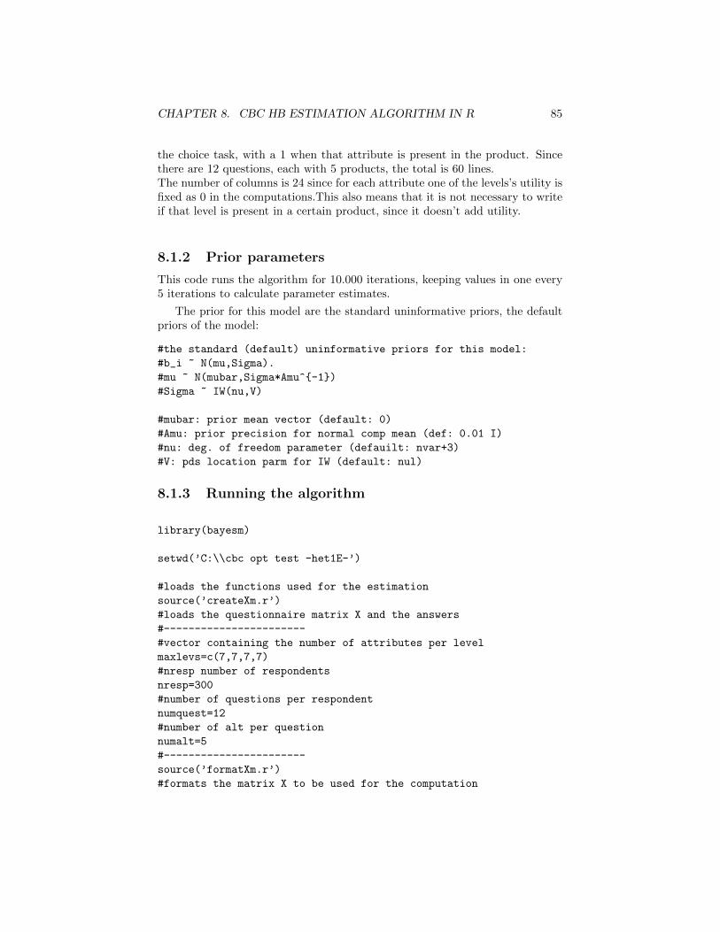
CHAPTER 8. CBC HB ESTIMATION ALGORITHM IN R 85
the choice task, with a 1 when that attribute is present in the product. Sincethere are 12 questions, each with 5 products, the total is 60 lines.The number of columns is 24 since for each attribute one of the levels’s utility isfixed as 0 in the computations.This also means that it is not necessary to writeif that level is present in a certain product, since it doesn’t add utility.
8.1.2 Prior parameters
This code runs the algorithm for 10.000 iterations, keeping values in one every5 iterations to calculate parameter estimates.
The prior for this model are the standard uninformative priors, the defaultpriors of the model:
#the standard (default) uninformative priors for this model:
#b_i ~ N(mu,Sigma).
#mu ~ N(mubar,Sigma*Amu^{-1})
#Sigma ~ IW(nu,V)
#mubar: prior mean vector (default: 0)
#Amu: prior precision for normal comp mean (def: 0.01 I)
#nu: deg. of freedom parameter (defauilt: nvar+3)
#V: pds location parm for IW (default: nul)
8.1.3 Running the algorithm
library(bayesm)
setwd(’C:\\cbc opt test -het1E-’)
#loads the functions used for the estimation
source(’createXm.r’)
#loads the questionnaire matrix X and the answers
#-----------------------
#vector containing the number of attributes per level
maxlevs=c(7,7,7,7)
#nresp number of respondents
nresp=300
#number of questions per respondent
numquest=12
#number of alt per question
numalt=5
#-----------------------
source(’formatXm.r’)
#formats the matrix X to be used for the computation
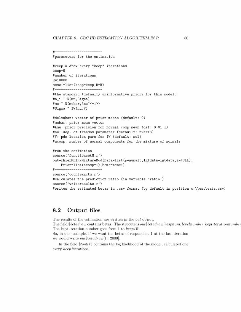
CHAPTER 8. CBC HB ESTIMATION ALGORITHM IN R 86
#-----------------------
#parameters for the estimation
#keep a draw every "keep" iterations
keep=5
#number of iterations
R=10000
mcmc1=list(keep=keep,R=R)
#-----------------------
#the standard (default) uninformative priors for this model:
#b_i ~ N(mu,Sigma).
#mu ~ N(mubar,Amu^{-1})
#Sigma ~ IW(nu,V)
#deltabar: vector of prior means (default: 0)
#mubar: prior mean vector
#Amu: prior precision for normal comp mean (def: 0.01 I)
#nu: deg. of freedom parameter (defauilt: nvar+3)
#V: pds location parm for IW (default: nul)
#ncomp: number of normal components for the mixture of normals
#run the estimation
source(’functionsetM.r’)
out=rhierMnlRwMixtureMod(Data=list(p=numalt,lgtdata=lgtdata,Z=NULL),
Prior=list(ncomp=1),Mcmc=mcmc1)
#-----------------------
source(’countexactm.r’)
#calculates the prediction ratio (in variable ’ratio’)
source(’writeresults.r’)
#writes the estimated betas in .csv format (by default in position c:\\estbeats.csv)
8.2 Output files
The results of the estimation are written in the out object.The field $betadraw contains betas. The strucute is out$betadraw[respnum, levelnumber, keptiterationnumber].The kept iteration number goes from 1 to keep/R.So, in our example, if we want the betas of respondent 1 at the last iterationwe would write out$betadraw[1, , 2000].
In the field $loglike contains the log likelihood of the model, calculated oneevery keep iterations.

Bibliography
[1] Bertolini M., Ofek E., Ariely D., The effect of Add-On features on perceivedproduct value, London Business School working papers, 2008.
[2] Chernev A., Hamilton R., Assortment Size and Option Attractiveness inConsumer Choice Among Retailers, Journal of Marketing Research, volumeXLVI.
[3] Dellaert B., Stremersch S., Marketing Mass Customized Products: Strikingthe Balance between Utility and Complexity, Journal of Marketing Research,August 2005.
[4] Evgeniou T., Pontil M., Toubia O., A fast optimization approach to robustheterogeneity modeling for choice-based conjoint estimation, http://w4.
stern.nyu.edu/ceder/research.cfm?doc_id=5402, 2005.
[5] Hastie T., Tibshirami R., Friedman J. The elements of statistical learning. Springer, second edition, 2009.
[6] Iyengar R., Jedidi K., Kohli R., A conjoint approach to multi-part pricing,Journal of Marketing Research, Vol. XLV, No. 2, April 2008
[7] Koop G., Bayesian Econometrics. John Wiley & Sons, 2003.
[8] Liechty J, Ramaswamy V., Cohen S., Bayesian econometrics, John Wiley& Sons, 2003.
[9] Liechty J, Ramaswamy V., Cohen S., Choice Menus for Mass Customiza-tion: An Experimental Approach for Analyzing Customer Demand withan Application to a Web-Based Information Service, Journal of MarketingResearch, Vol. XXXVIII (May 2001).
[10] Marder E., The assumptions of choice modelling: Conjoint analysis andSUMM, Canadian Journal of Marketing Research, Volume 18, 1999.
[11] Maxwell S. The price is wrong, John Wiley & Sons, 2007.
[12] Rossi E., Allenby G., McCulloch R., Bayesian statistics and marketing,John Wiley & Sons, 2005.
87

BIBLIOGRAPHY 88
[13] Sawtooth Software, The CBC/HB system for Hierarchical Bayes estimation- version 4.0, http://www.sawtoothsoftware.com/, 2005.
[14] Solomon M., Bamossy G., Askegaard S., Hogg M., Consumer behavior - anEuropean perspective, Prentice Hall, third edition, 2006.
[15] Train K., Discrete Choice Models with Simulation, Cambridge UniversityPress, 2003.
[16] Wooldridge J.M., Econometric analysis of cross section and panel data,MIT Press, 2002.