Discrete Element Modelling

in STAR-CCM+ Oleh Baran

DEM overview

DEM capabilities in STAR-CCM+

– Particle types and injectors

– Contact physics

– Coupling to fluid flow

– Coupling with passive scalar

Performance and scalability

Simulation assistant benefits

Scaled particle approach

Summary

Outline

2

DEM is applicable to solid flows

– When part or whole solid phase is in dense shear flow regime

– With particles of different shape and size distribution

DEM for particle flow with resolved collisions

3

DEM examples

4

Momentum conservation

𝑚𝑖𝑑𝑣𝑖𝑑𝑡= 𝐹𝑖𝑗 + 𝐹𝑔 +

𝑗

𝐹𝑓𝑙𝑢𝑖𝑑

𝑚𝑖 and 𝑣𝑖 are mass and velocity of particle 𝑖, 𝐹𝑔 = 𝑚𝑖𝑔 is gravity force, 𝐹𝑖𝑗 is

contact force between particle 𝑖 and element 𝑗

- DEM is a meshless method!

- DEM is computationally intensive method!

Conservation of angular momentum 𝑑

𝑑𝑡𝐼𝑖𝜔𝑖 = 𝑇𝑖𝑗

𝑗

– 𝑖, 𝐼𝑖 and 𝜔𝑖 are the momentum on inertia and rotational velocity of particle 𝑖. 𝑇𝑖𝑗 = 𝑟𝑖𝑗(𝐹𝑖𝑗 + 𝐹𝑟) is the torque produced at the point of contact and it is the

function of the rolling friction force 𝐹𝑟

DEM Governing Equations

5

Base model is non-linear Herz-Mindlin model

– Details in Di Renzo, A., & Di Maio, F. P. (2004). Comparison of contact-force models for the simulation of collisions in DEM-based granular flow codes. Chemical Engineering Science, 59, 525 –541

– Other models available (next slide)

The normal and tangential components, 𝑭𝒏 and 𝑭𝒕,of contact force depends on overlap, particle properties

– Young’s modulus

– Density

– Size

– Poisson ratio,

– and interaction properties, for example friction, rolling friction, restitution, etc

DEM in STAR-CCM+ overview: Contact Forces

6

Basic models

DEM Capabilities: Contact models

Hertz-Mindlin Classical nonlinear contact force model for

rigid bodies

Friction, restitution (normal

and tangential)

Walton-Brawn Linear model for deformable particles Compression and tensile

stiffnesses

• Optional models (for adding to basic model)

Rolling

Resistance

Force proportional Set of rolling friction

parameters Constant Torque

Displacement Damping

Linear Cohesion Constant attractive force matching either JKR

force or DMT model for zero overlap

Work of cohesion,

model blending factor

Artificial Viscosity Additional velocity dependent damping model Linear and Quadratic

coefficients

Parallel Bonds For modelling consolidated particles Max tensile and shear

stress, Bond radius

Conduction Heat

transfer

For both particle-particle and particle-geometry

contacts

Ranz-Marshall or user

set heat transfer 7

Particle Type

Spherical

Composite Rigid, unbreakable

Clumps Flexible, breakable

Particle

Initialization

Volumetric injection

• Random Injector: on region or Part

• Random injector

• Lattice injector:

• Part injector: on volume cells

Surface injection Surface or Part Injector: on boundary

cells, or on planar grid

All injectors : - ability to set particle size distributions: constant, normal, log-normal, other

- ability to specify flow rate, initial velocities, orientation, etc

DEM- Capabilities: Particles

8

DEM Coupling to Fluid Flow

Drag Force

Di Felice

Schiller-Naumann

Gidaspow (for 2-way coupling only)

User defined field function

Drag Torque With either Sommerfeld Rotational Drag or user

defined rotational drag coefficient

Lift Force

Shear Lift: Choice of Saffman, Sommerfeld, user-set

coefficients

Spin Lift: Choice of Sommerfeld or user-set

coefficients

Pressure Gradient

Force Buoyancy force

Two-way coupling Fluid is affected by particles: Momentum source is

applied to continuous phase

Other interactions Gravity force, User-Defined Body Force, Particle

Radiation, Energy model, Passive Scalar

9

New in version 8.06

Arbitrary number of new particle properties

– Color

• Tracing subset of particles

• Analyzing mixing efficiency

– Particle residence time or displacement

• ‘dead zone’ or ‘risk zone’ analysis of granular flow

– Coating amount

• Residence time in user-defined ‘spray zone’

– Wetness / dryness of particles

• Contribution from several processes

– Amount of chemically active component

Can interact with Eulerian passive scalar

DEM Passive Scalar

10

Passive scalar for binning and mixing

11

Source term:

$${ParcelCentroid}[0] * $ParticleDensity *

$TimeStep * ($Time > 0 ? 0 : 1)

Source term:

($${ParcelCentroid}[0]<0) ? 0 : 1)

Challenge: Improve inter-particle coating uniformity by using optimal spraying equipment settings – Solution: using DEM passive scalar capability

Passive scalar source: ($$ParcelCentroid("Cyl")[2] > 0.0 && $$ParcelCentroid("Cyl")[2] < 0.22 && $$ParcelCentroid("Cyl")[0] < 0.05+1.12*$$ParcelCentroid("Cyl")[2] ) ? 0.1*$ParticleDensity : 0.0

– Coating thickness is accumulated in ‘spray zone’

– Single simulation provides solution for two different spray methods

Passive scalar for coating applications

12

Passive scalar: Lagrangian-Eulerian coupling

Example of particles in a pile ‘releasing

‘gas

– Left Inlet air flow 100 m/s, later 10 m/s

– Particles initialized with non-zero

‘Particle Gas’ value of passive scalar 𝜙1

– Eulerian passive scalar 𝜙2 has diffusion

and convection on, initial value zero in

all cells

– Volume weighted interaction model for

flow rate between passive Lagrangian

and Eulerian scalars:

• 𝐽 = 𝑘 𝜌1𝜙1 − 𝜌2𝜙2 𝐴𝑝 here 𝑘 = 0.01 is

user controlled interaction coefficient, 𝜌1 and 𝜌2 are densities of Lagrangian and

Eulerian phases, 𝐴𝑝 is the surface area of

the particle

13

Performance and Scalability

Performance-improving features:

– Load Balancing

– Per-continuum parallel solver

– Maximum Independent Set

Algorithm in injectors

– Skinning

Typical simulation time of Fluidized

bed in version 8.02:

1 s Physical time for 28 h / 118 CPU

for 1.3 millions of particles

d=2 mm, ρ=2440 kg/m3, E=10 MPa

14

DEM timestep

~𝑑𝜌

𝐸

Material density of least dense phase 𝜌

Diameter of smallest sphere 𝑑

Young’s Modulus of hardest particle 𝐸

DEM Solver Timescale

Number of

elements

Total Number of spheres

Number of CPU

Number of faces in mesh

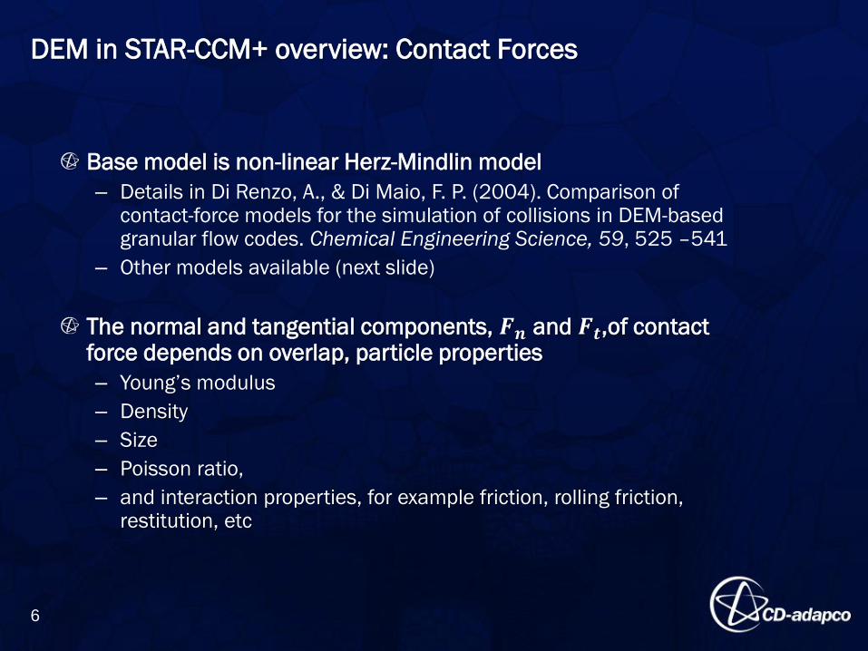
Max Physical time

Skinning

15

Contact detection optimized

– New skin parameter in DEM solver

– the larger the skin distance, the less often neighbor lists need to be re-built,

• but more pairs must be checked for possible force interactions inside one neighborhood

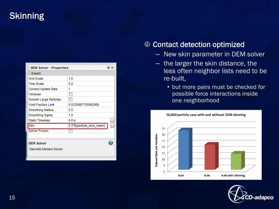
Simulation Assistant Benefits

16

Can we use ‘larger particles’ to reduce particle count without significant

change in accuracy of the model?

– In particular for fluidized bed application?

fine particles of size 𝑑0 scaled-up particle of size 𝑑

Suggested correction to Gidaspow drag coefficient

𝐶𝑑 ⇒𝑑

𝑑0

𝑛

𝐶𝑑

Scaled Particle Approach

17

Fluidized bed set up

18

J. X. Bouillard, R. W. Lyczkowski and D. Gidaspow, "Porosity Distributions in a Fluidized

Bed with an Immersed Obstacle," AIChE Journal, vol. 35, no. 6, pp. 908-921, 1989

- Size of particles – 0.503 mm

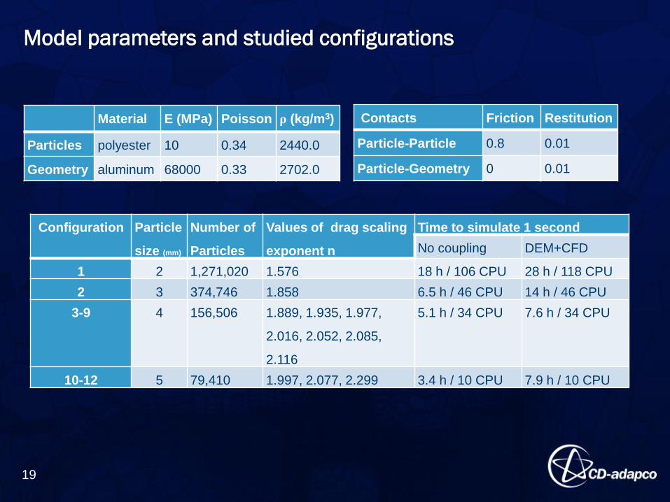
Model parameters and studied configurations

Configuration Particle

size (mm)

Number of

Particles

Values of drag scaling

exponent n

Time to simulate 1 second

No coupling DEM+CFD

1 2 1,271,020 1.576 18 h / 106 CPU 28 h / 118 CPU

2 3 374,746 1.858 6.5 h / 46 CPU 14 h / 46 CPU

3-9 4 156,506 1.889, 1.935, 1.977,

2.016, 2.052, 2.085,

2.116

5.1 h / 34 CPU 7.6 h / 34 CPU

10-12 5 79,410 1.997, 2.077, 2.299 3.4 h / 10 CPU 7.9 h / 10 CPU

Material E (MPa) Poisson ρ (kg/m3)

Particles polyester 10 0.34 2440.0

Geometry aluminum 68000 0.33 2702.0

Contacts Friction Restitution

Particle-Particle 0.8 0.01

Particle-Geometry 0 0.01

19

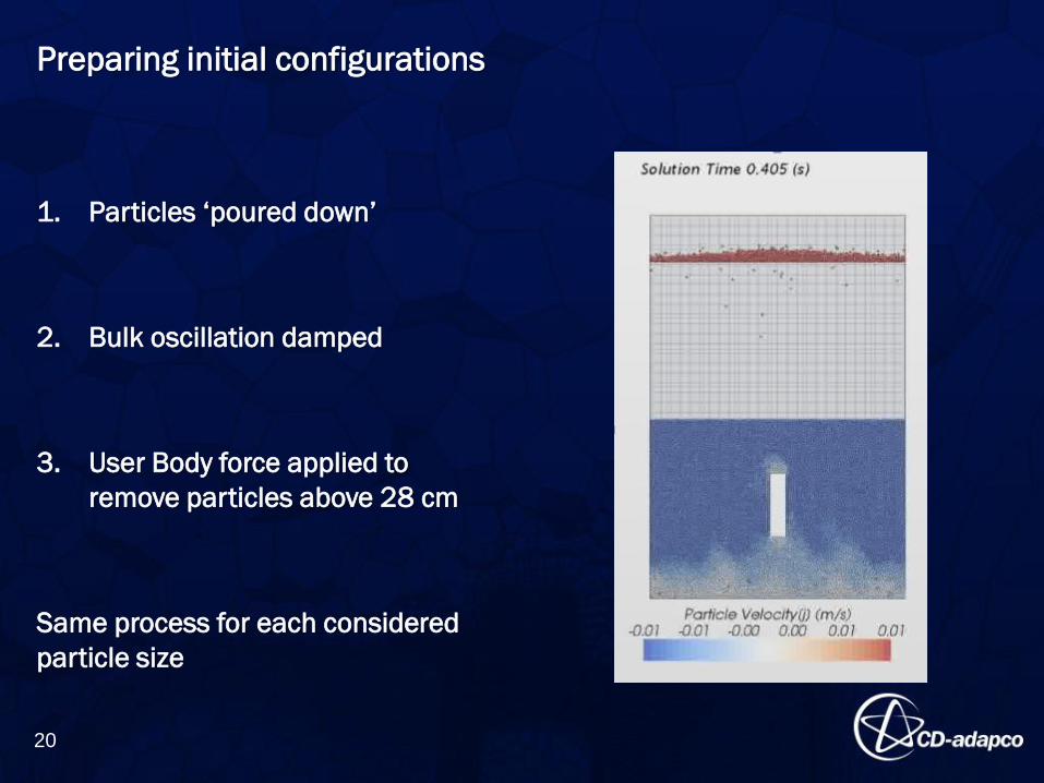
Preparing initial configurations

1. Particles ‘poured down’

2. Bulk oscillation damped

3. User Body force applied to

remove particles above 28 cm

Same process for each considered

particle size

20

Pressure drop calculations

Two way-coupling activated

– All three inlets set to have same

inlet velocity

– Superficial velocity 0.0989 m/s

Simulated at least 0.5 s in steady

state

Pressure drop recorded

Same process for all 12

configurations

21

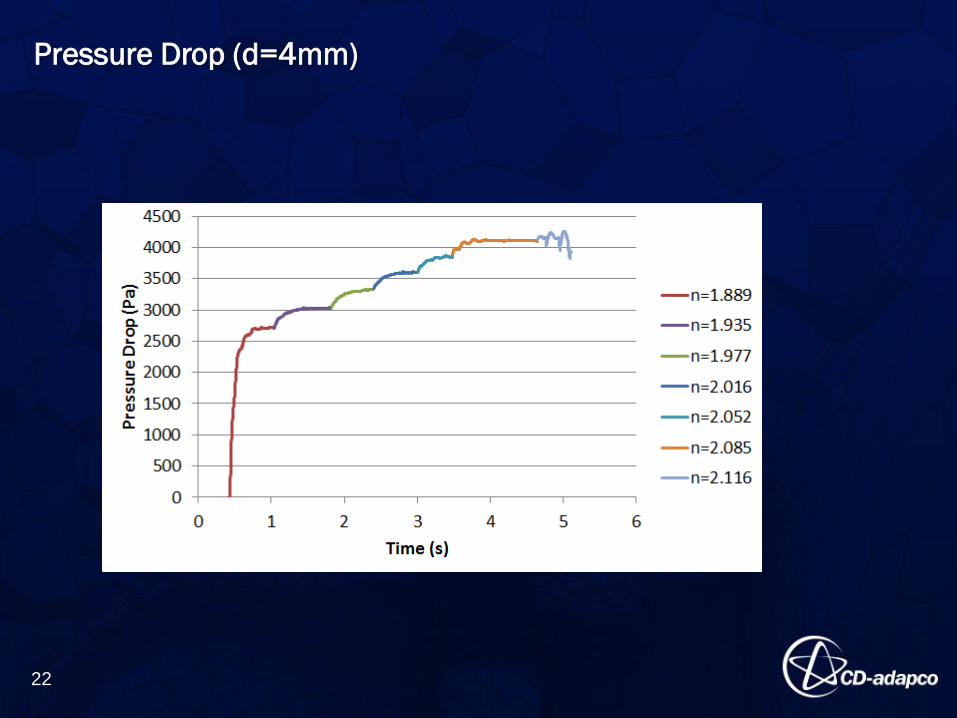
Pressure Drop (d=4mm)

22

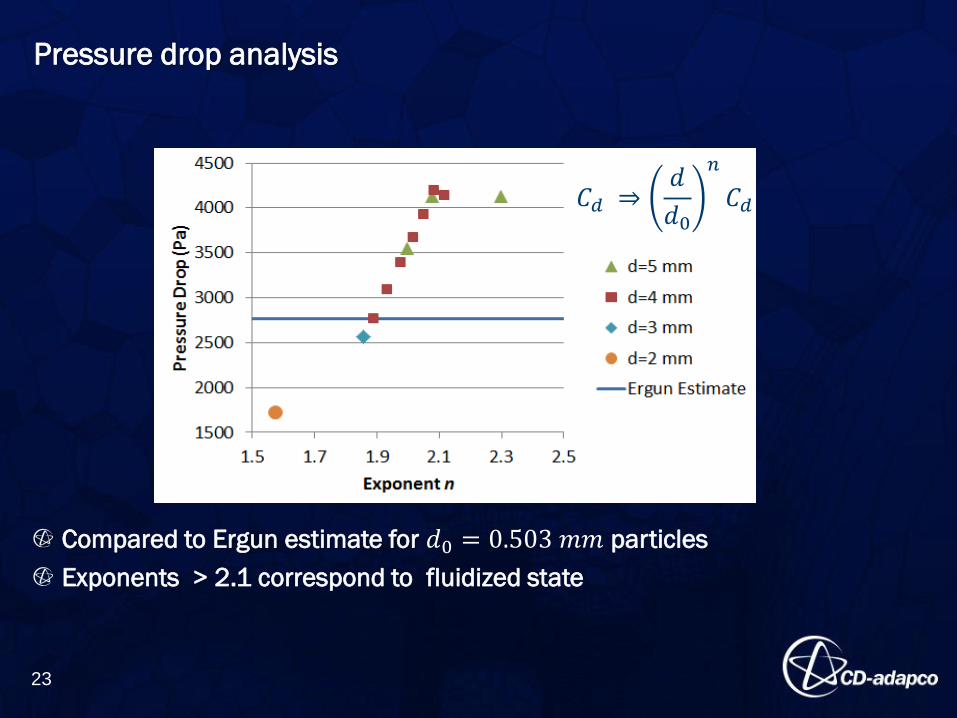
Pressure drop analysis

Compared to Ergun estimate for 𝑑0 = 0.503 𝑚𝑚 particles

Exponents > 2.1 correspond to fluidized state

23

𝐶𝑑 ⇒𝑑

𝑑0

𝑛

𝐶𝑑

Simple power-law correction to drag force was used for scaled particles

Results for pressure drop collapsed on single curve

– Perhaps limited for the particular choice of model parameters

• Low coefficient of restitution

• Further investigations are underway

– More accurate scaling can be set from force balance

• Sakai et. al., Study of a large scale discrete element model for fine particles in a

fluidized bed, Adv. Powder Technology 23 (2012) 673-681

Scaled particles can provide same pressure drop for less computation

time

Summary of fluidized bed study

24

Thank you!

25

Back-up slides

26

Void fraction

27

d=3mm

Initial d=3mm

Final

d=4mm

Initial d=4mm

n=1.9

d=4mm

n=2.1

(fluidized)

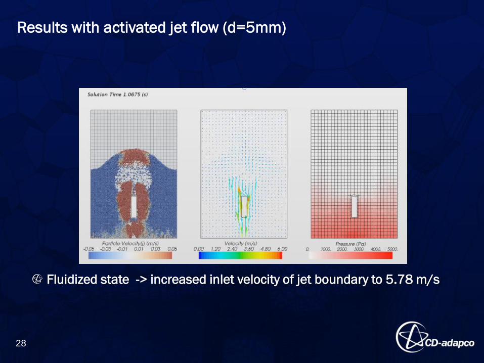
Results with activated jet flow (d=5mm)

Fluidized state -> increased inlet velocity of jet boundary to 5.78 m/s

28

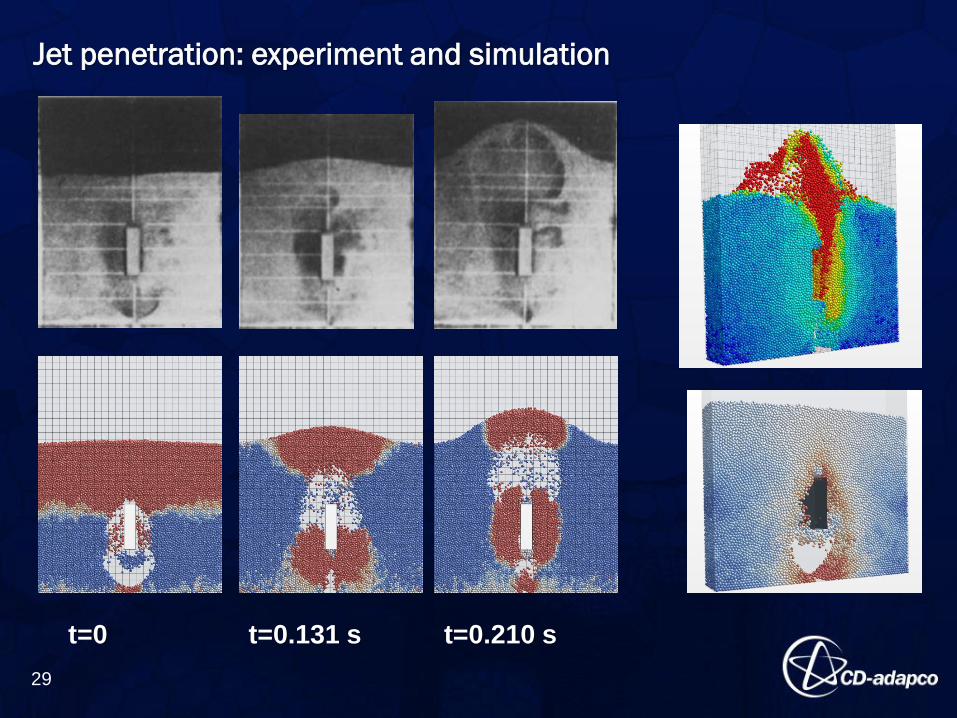
Jet penetration: experiment and simulation

29

t=0 t=0.131 s t=0.210 s

Time and space average solid velocity

d=5 mm

17 x 23 bins

– 25.4mm x 25.4mm x 76.2mm

Averaged over 2 s

30