Discrete Fracture Method for Petroleum Reservoir ... · Discrete Fracture Method for Petroleum Reservoir Simulation Using an Element-based Finite Volume Method C.R. Maliska* (Federal

ECMOR XV - 15th European Conference on the Mathematics of Oil Recovery

29 August – 1 September 2016, Amsterdam, Netherlands

Mo P038Discrete Fracture Method for Petroleum ReservoirSimulation Using an Element-based FiniteVolume MethodC.R. Maliska* (Federal University of Santa Catarina), B.T. do Vale (FederalUniversity of Santa Catarina) & F. Marcondes (Federal University of Ceará)

SUMMARYAny porous media flow is inherently complex to model due to the impossibility of giving the real flowgeometry to the simulation model. If heterogeneous media is involved, as is the case of naturally fracturedpetroleum reservoirs, the difficulty increases even more, since large fractures can be seen asdiscontinuities, having as background the porous matrix, in which many smaller sized fractures arepresent. The porous matrix can be treated by a stochastic procedure and are, normally, large deposits of oil,while the large fractures are better solved through a deterministic treatment. A network of connected largefractures linked to the porous matrix may be the most important flow path for oil production. In the otherhand, depending on the physical properties, capillarity and permeability, the fractures and porous matrixcombination may lead to a undesirable secondary oil recovery, leaving considerable amount of oil in theporous matrix. Therefore, the prediction of this combined flow (fractures +porous matrix) is of utmostimportance for the oil industry. There are several approaches to solve this combined flow, all of thembased, of course, on a idealized fracture configuration, which gets more and more realistic as thecharacterization methods evolves, due to the specialization of well-logging, 4D seismic and other methods.The final goal would be to solve the local flow for any single fracture, irrespective its size, nowadays animpossible task due to the lack of characterization methods and computer capacity. However, ascomputational power and characterization techniques evolve, methods able to solve the details of the flowshould be devised. This paper follows this route and presents a DFM (Discrete Fracture Method) in theframework of an Element-based Finite Volume Method (EbFVM) using unstructured grids. The EbFVM isper se a multi-point flux approximation, avoiding the usual two-point approach, which is conceptuallywrong, since the errors do not vanish as the grid is refined. The EbFVM also avoids the need of morecomplex MPFA algorithms for having correct flux evaluation. Additionally, the EbFVM framework allowsthe use of truly directional upwind and higher order schemes with no extra efforts.The 2D oil-water flow using the DFM method with superposition for connecting the fractures and theporous matrix is solved. The fractures are assumed to be 1D considering its real thickness. Several aspectsof the model are investigated, as the capillarity effects, especially in the situation in which imbibition ofthe porous matrix occurs and the anisotropy of the coefficients of the linear system resulting from thesuperposition of the equations. Since IMPES method is used, comments on the time step adaption is alsogiven.



Introduction In the last decades, driven by the growing demand for oil, the study of naturally fractured reservoirs has received a lot of attention. Due to complex tectonic movements and sedimentation processes, natural fracture reservoirs have a great complexity in his characterization; there exist two different media for fluid flow transport: fractures and matrix. Fractures present distinct hydraulic conductivity and capillary effect from the matrix, and they can be characterized as discontinuities in the porous matrix. According to Kaul et al. (2004), the main issue in the analysis of discrete fracture reservoirs lies in the interaction between these two different media and the properties that affect the flow, especially capillarity and gravity, which makes the phenomenon difficult to quantify.

In a naturally fractured reservoir, fractures or natural cracks are largely responsible for fluid transport through the reservoir, with high permeability and low capacity for fluid storage (the relationship between the volume of the fractures and total rock volume is around 1%). The rock-matrix or simply matrix has low permeability (0.01 to 1 mD), but presents high capacity for storing of fluids (Rosa et al., 2006), and therefore work as a fluid feeding for the fractures. However, for fractures to act as a main transport media, it is expected that they are connected to each other. Therefore, not only the discrete fractured connectivity, but also their distribution and properties need to be known in order to properly determine the fluid flow (Long and Witherspoon, 1985). This fact becomes even more pronounced in situations where multiphase flow occur, since each phase can have a different flow pattern. According to Monteagudo and Firoozabadi (2004) fractures can be the main media for some components and the matrix for the others.

According to Li and Lee (2008), full knowledge of the reservoir fractures distribution is almost an impossible task, since the fracture system is quite irregular and often disconnected. Geologists use different information to synthesize the fracture distribution such as well production profiling, pressure well tests, images, and core samples of the reservoir. In general, data on fractures are provided statistically through distribution functions for the thickness, length, and orientation, among other characteristics. Although they apparently have a random behavior, it is common to find real field situations where fracture are oriented in a preferred direction, since fractures tend to occur in planes perpendicular to the lower direction of the rock stress.

The main goal of the present work it to investigate the secondary recovery process by water injection in natural fractured reservoirs in conjunction with 2D-unstructured grids, and using the framework of the Element-based Finite-Volume Method (EbFVM) which, by its turn, facilitates the numerical integration of the fracture with the matrix. Simulation of naturally fractured reservoirs In order to analyze the secondary recovery process in natural fractured reservoirs several experimental studies have been conducted (Horie et al., 1990; Pooladi-Darvish and Firoozabadi, 2000; Hirasaki and Zhang, 2004). Although these studies provide important results, numerical simulation is still an important tool to better understand the fluid flow in naturally fractured reservoirs. In this scope, one possible representation that gives accurate results regardless the fracture network is called simple fracture porosity model. As presented by Phelps et al. (2000) and Dogru et al. (2001), in this model one has the explicit discretization of the discrete fractures into the grid of the reservoir. That is, the grid has elements for both discrete fractures and matrix. Due to the large discrepancy between the two media (discrete fracture and matrix), rock properties as porosity and permeability are discontinuous and present sharp variations. Although this formulation provides accurate results, it is computationally expensive since a large amount of elements are required to represent both media. In addition, local grid refinement are, in general, also required, which cause large variation in the size of the grid.



Figure 1 shows an example of grid used by this formulation. Other formulations used to model the fluid flow in natural fracture reservoirs are described in the next sections.

Figure 1 – Grid example used in the simple fracture model

Equivalent porous media model

In this group are the methods that try to represent the natural fractured reservoir as a single continuous medium by changing the physical properties. One of the first works in this area was performed by Hsieh and Neumann (1985), which attempted to represent a system where the flow was only through the fractures by using a volumetric average of the absolute permeability of both media. This method, however, is not restricted to situations where the matrix is isolated. This homogenization of the properties is suitable for media with high degree of fracturing. In this methodology, special attention should be given to the representative elementary volume (REV), which is the minimum volume of rock that can be considered representative of the fractured medium. Naturally fractured reservoirs can present high REV values, which initially prevents the choice of homogenization. Neuman (1988) used a stochastic approach to turn the homogenization independent of REV value. Although this model can be easily used, it has an important drawback since physical properties of the medium are generalized, and thus important features of the discrete fractures are hidden. Van Lingen et al. (2001) proposed the use of pseudo relative permeability curves for grid blocks containing fractures in order to analyze the fractured and matrix media as one medium, and hence avoiding local gridding refinement or unstructured grids. This approach differs from the homogenization of the properties, since Van Lingen et al. (2001) proposed changes in porosity and absolute permeability, and also adopted pseudo relative curves for capillary pressure and relative permeability for the grid blocks that are crossed by fractures, in order to consider and represent both the fluid flow into the fractures and exchanges with the matrix. This adaptation greatly restricts the flexibility of this model. Such effect occurs because pseudo parameters, in particular, for the relative permeability curves can hardly be determined, since they depend on all factors controlling the exchanges between the matrix and fractures. The pseudo curves approach is indicated for situations where large amount of flow occurs in the matrix. Multiple domain models In this classification are the methods that represent matrix and discrete fractures separately, and a fluid transfer function is used to connect both media. In this category, the most used model in the petroleum industry is the dual porosity model, which was proposed by Barenblatt et al. (1960) for slightly compressible single-phase flows. For each medium, phase saturation and pressure were considered as unknowns. The mass exchange between both media was modeled through a transfer function for the pseudo static regime such the material balance between both media was satisfied. Using an analytical solution for radial, single-phase flow Warren and Root (1963) presented a practical model assuming that the grid blocks are uniform and homogeneous, isotropic, and



rectangular sugar cubes limited by the fracture planes, which is shown in Figure 2. Besides the simplifications just mentioned, the authors also made some adjustments in the flow equations of the problem. For instance, they assumed that the flow occurs only through the fracture network, and the matrix storages the fluid only, and hence feeding the flow from matrix to the fracture network through the transfer function. The methodology proposed by Warren and Root (1963) became well known in the petroleum literature as dual porosity model, and several improvements have been performed in the transfer function by several authors, which are described next in this section.

Figure 2 – Description of dual porosity model

Kazemi et al. (1976) generalized this model for a two-phase flow with gravitational and relative mobility effects. Thomas et al. (1983) developed a three-dimensional, three-phase model, where the pseudo relative permeability curves were included in the transfer function. For the aforementioned methods, there is no communication between the matrix grid blocks. This simplification is allowed for cases where there is not a significant flow in the matrix. The dual permeability model (or dual porosity-dual permeability) was developed to represent cases where this assumption is not possible. Blaskovich et al. (1983) and Hill and Thomas (1985) generalized the dual porosity model to establish connections between the matrix grid blocks and fractures, and therefore allowing mass exchange between them. The multiple domain models are ideal for highly fractured reservoirs composed of small and connected fractures. Although not restricted to this case only, this methodology has some severe limitations. First, the determination of the transfer function between fracture and matrix is a complex task, since it depend on several properties of the porous media. Furthermore, the uniformity of geometry and properties can hide important parameters of fracture network, such as thickness, length, connectivity, direction, and spacing, which as previously discussed, interfere effectively in the fluid flow. Concerning the geometric representation of fracture network, some research has been performed to ensure greater flexibility. In order to better described the transient fluid flow of the matrix domain, Naimi-Tajdar (2005) proposed a discretization of both horizontal and vertical matrix grid blocks. Discrete fracture model In order to better represent the fluid flow in the discrete fracture model, the properties of fractures such as connectivity, direction and thickness are considered. Some authors like Gong (2007), consider that the single porosity model is actually a discrete fracture model. However, in this work, what is considered in this classification it is a simplification of single porosity model. If we compare the multiple domain model, which simplifies the geometry to highlight the flow modeling, the discrete fracture model focus on the opposite direction; here the main concern is with the geometry of the fracture network, but, in general, using a simplified physical model (La Pointe et al., 1997). Figure 3 shows how the discrete fractures are represented in this method. Based on different approaches, there



are two types of discrete fracture models: the unstructured discrete fracture model (USDFM) and the embedded discrete-fracture model (EDFM) (Moinfar et al., 2011 and Moinfar et al., 2012).

Figure 3 - Representation of discrete fracture model The pioneering works using the USDFM for simulating single phase flow in two-dimensional geometries were performed by Noorishad and Mehran (1982) and Baca et al. (1984). To represent properly the fracture network, unstructured grids were used, and the fractures were aligned along the edges of the elements of the grid. Therefore, the fluid flow into the matrix is 2D, while the fluid flow into the discrete fracture is 1D. Karimi-Fard and Firoozabadi (2001) showed that this simplification did not affect the accuracy of the results when compared with the simple porosity model. In this methodology, the matrix and fractures are coupled using the superposition principle, i.e. each medium is discretized separately, and then the balance equations of each media are added in order to obtain the final equation denoting the material balance of both media. Kim and Deo (2000), Karimi-Fard and Firoozabadi (2001), and Monteagudo and Firoozabadi (2004) expanded the original concept of USDFM by adding the effect of capillary pressure for the simulation of incompressible multiphase flows. Compared to the explicit representation of the fractures, the USDFM dramatically reduces the simulation time. It is a more realistic representation of the fracture network by considering the effect of each fracture on the fluid flow. Moreover, as it applies the principle of superposition, there is no need for calculating the transfer function to connect both media, once the equations of both media are summed up, the transfer functions of each media vanished when the equations are added together. The USDFM presents some drawbacks. First, if the number of discrete fractures increases, the number of elements of the grid increases in a non-linear way. In addition, this model usually generates a high level of anisotropy in the coefficients of the linear system of equations, which makes its solution difficult (Moinfar et al. 2011). The EDFM approach was originally proposed by Lee et al. (2001), and was later explored by Li and Lee (2008) and Moinfar et al. (2012). One advantage of EDFM approach when compared to the USDFM is the possibility to use structured grids and hence there is no need to perform local grid refinement, since in this approach there is no flow modelling around the fractures. In order to model the flow between the fractures and matrix, an analogy with the procedure for coupling wells to grid blocks is performed. The concept of the well index introduced by Peaceman (1978) is used to obtain similar equations for coupling the fractures to the matrix. The early works assumed vertical fractures. Moinfar et al. (2012) extended the method to model inclined fractures. Although EDFM is computationally cheaper than USDFM, the high computational cost of the EDFM still persist when the number of discrete fractures is increased. The discrete fracture model is particularly suitable for situations where the rock-matrix has very low intrinsic permeability, or the fracture network determines how the fluid flow occurs.



Mathematical modelling This section presents the conservation equations for the fluid flow problem, the model for relative permeability and capillarity and the discrete fracture approach. Two-phase fluid flow problem The governing equations for fluid flow in porous media are given by the mass, momentum, and energy equations. In a porous media, the momentum equation of each phase is usually replaced by the Darcy’s law. In this work, we will deal with isothermal, immiscible, incompressible two-phase flows in natural fractured reservoirs. These hypotheses are commonly associated with the secondary recovery in petroleum reservoir simulations. Since only isothermal flows will be considered, the problem described next in this section can be fully described by one elliptic equation for pressure, and a hyperbolic equation for saturation. Assuming immiscible fluid flow, the mass balance for phase α can be written as

∂∂t ραSαφ( ) =−∇. ραuα( )+qα , (1)

where ρα and Sα denote respectively, the mass density and saturation of phase α, φ denotes the porosity of the porous medium, qα denotes the volumetric rate per volume of rock plus void space,

and αu denotes the velocity vector of phase α, which is given by Darcy’s law for multiphase flow by

.rk Kαα α

αμ=− ∇Φu ,

(2)

where K is the absolute permeability tensor of the medium, krα and μα respectively denote the relative permeability and dynamic viscosity of phase α, and αΦ denotes the potential of phase α. This potential can be written as a function of phase pressure and a gravity term, as

P g zα α αρΦ = + (3)

In Eq. (3), Pα is the pressure of phase α, z is depth, which is positive in the upward direction, and g is the gravitational acceleration. Since only two-dimensional simulation will be treated in this work, there is no variation in z-direction and therefore, one can rewrite Eq. (1) as,

∂∂

ραSαφ( ) =∇. ραλα K .∇Pα( )+qα ,(4)

where αλ denotes the ratio of relative permeability to the viscosity of phase α. Assuming incompressible fluid and porous medium, one can write Eq. (4) as

( ). .S K P qtα

α α αφ λ∂ =∇ ∇ +∂

,(5)

where



qα =

qα

ρα

(6)

Being pressure and saturation of each phase as unknowns of the problem, there are two equations (mass conservation equation for each phase, Eq. (5)) and four unknowns (Po, Pw, So, Sw). The two closure equations come from the volumetric restriction that can be written as

1o wS S+ = , (7) and from the experimental data through the definition of capillary pressure (Pc),

o w cP P P− = . (8)

Although there are four unknowns, in practice only two equations are discretized: Eq. (5) is used to obtain Sw. To evaluate Pw, the mass conservation is written for the oil and water phase, and summed up. Such procedure results, after some algebraic manipulations, in the following equation

( ) ( ). . . .t w o c tK P K P qλ λ−∇ ∇ − ∇ ∇ = , (9)

where the total mobility (λt = λo + λw) and qt = qo + qw. Po and So are obtained from the closure equations. Models for the relative permeability and capillary pressure

For the two-phase flow (oil-water) of this work one assumes the water phase is the wetting phase. While the absolute permeability is an intrinsic property of the rock, the relative permeability depends on the interactions between fluid and media, and it is usually calculated as a function of saturation. There are several models to describe the behavior of the relative permeability curves. The Corey model (Corey, 1954) is used in this work. The expression for the relative permeabilities of water and oil are given by

1

wn

w wirw rwor

wi or

S Sk kS S

⎛ ⎞−= ⎜ ⎟− −⎝ ⎠,

(10)

11

on

w orro rowi

wi or

S Sk kS S

⎛ ⎞− −= ⎜ ⎟− −⎝ ⎠,

(11)

where Swi and Sor denotes the irreducible water saturation and residual oil saturation, respectively, krwor is the water relative permeability at the point where the oil saturation is equal to Sor, krowi is the oil relative permeability at the point where the water saturation is equal to Swi, nw and no are the Corey’s exponents for the water and oil phases, respectively. Figure 4 shows the curves used for water and oil, with all the parameters presented in Eqs. (10) and (11). For capillary pressure, it is adopted the same model used by Monteagudo and Firoozabadi (2004), given by

( ) lnc w wP S B S=− , (12)



where B is a constant. The capillary pressure decreases as water saturation increases; it vanishes if the water saturation is equal to unit and tends to infinity if water saturation approaches zero. In order to prevent an infinite value, one sets a maximum value for the capillary pressure obtained when Sw = 0.001.

Figure 4 - Relative permeability curves for the Corey’s model

Discrete fracture model In this work, we employs the USDFM methodology initially presented by Monteagudo and Firoozabadi (2004). As previously mentioned, the final equations are obtained using the superposition principle. According to this, the fractured domain can be decomposed as

m fεΩ=Ω + Ω , (13)

where mΩ and fε Ω denote the matrix and fracture sub-domains, respectively, and ε is the fracture aperture. For each media, considering the different dimensions, the following set of equations for the matrix (m) and fracture (f) are obtained: Pressure equation for the wetting phase for the rock-matrix:

−∇⋅ λt

mKm∇Pwm( )−∇⋅ λo

mKm∇Pcm( ) = qt

m . (14)

Saturation equation for the wetting phase for the rock-matrix:

( )φ λ∂∂

−∇⋅ ∇ =m m m m mww w

m

w

SP

tq .

(15)

Pressure equation for the wetting phase for the fracture:

K Kλ λ∂ ∂∂ ∂∂ ∂ ∂

⎛ ⎞ ⎛ ⎞− − =⎜ ⎟ ⎜ ⎟

⎝ ⎠ ⎝ ⎠∂f f f f fwt o

f fc

t

P Pw w w

qw

.(16)

Saturation euation for the wetting phase for the fracture:



Kφ λ∂ ∂∂ ⎛ ⎞− =⎜ ⎟

⎝ ⎠∂ ∂ ∂f f f fw w

f

w w

fPtS

qw w

.(17)

For the fracture equations, the ω letter indicates the discrete fracture orientation. From Eqs. (14) through (17), it is possible to observe that saturation and pressure from both media (matrix and fracture) can present different values. This assumption distinguishes the work of Monteagudo and Firoozabadi (2004) from the other works associated with the USDFM method mentioned above. In order to this hypothesis be valid is necessary to couple the unknowns of both media. Here we assume that the potentials of each phase at the discrete-matrix interface are equal. Such definition imply that that capillary are also equal,

Pc

m Swm( ) = Pc

f Swf( ) . (18)

With this consideration, one can relate the saturations in fracture and matrix as shown in Figure 5. Attention should be given to fact that the relative permeabilities of fracture and matrix at the interface between the two media may be different due to the parameters of each model, and also to the discontinuity of saturation at the interface of both medium.

Figure 5 - Capillary pressure and relationship between the saturations at the

matrix-fracture interface Applying the chain rule to the accumulation term of Eq. (17), one obtains

∂Swf

∂t=

dSwf

dSwm

∂Swm

∂t. (19)

Using Eq. (19), the final form of the fracture equations can be written in terms of the unknowns of the matrix, as Pressure equation for the wetting phase for the fracture:

K Kλ λ∂ ∂∂ ∂∂ ∂ ∂

⎛ ⎞ ⎛ ⎞− − =⎜ ⎟ ⎜ ⎟

⎝ ⎠ ⎝ ⎠∂f f f f fwt o

m mc

t

P Pw w w

qw

. (20)

Saturation equation for the wetting phase for the fracture:

( ) 1 Kφ λ

− ∂ ∂∂ ⎛ ⎞− =⎜

⎝ ⎠∂ ∂ ⎟∂

m

fB mm

f m f f fw wBw w wf

mPt w wSB

S qB

. (21)



Further details about the model can be found in Monteagudo and Firoozabadi (2004). Numerical Modelling The Element-based Finite Volume Method- EbFVM The EbFVM - Element-based Finite Volume Method is employed in this work for obtaining the approximate equations. Several methods akin to EbFVM have been recently used for treating fractured reservoirs (Matthai et al., 2007; Monteagudo and Firoozbadi, 2004; Benedetto et al., 2015; Haegland et al., 2009), among others. The EbFVM, was introduced in the 80’s (Baliga and Patankar, 1980) named CVFEM - Control Volume Finite Element Method, a denomination which, in some extent, conveys the reader to see the method as a Finite Element Method (FE). It is in fact a pure Finite Volume Method (FV) with no relations with traditional FE techniques. It only borrows from FE the concept of elements (not existing in FV methodologies prior to the use of unstructured grids). Triangles and squares in 2D, and tetrahedrons, hexahedrons, prims, and pyramids in 3D are elements that can be used in a FE or FV methodologies. In a FV approach if the element coming from the grid generator is used as control volume, the method is called a cell-center method, while if the control volume is created using parts of the element sharing the same node, it is called a cell-vertex method. The EbFVM belongs to the later category and is, inherently, a multi-point flux approximation due to the construction of the corresponding control volume. There is no need of creating interaction regions as done in the several types of MPFA methods for including the neighboring points in the flux calculation. And being a multi-point flux approximation, it avoids the use of only two-point for the flux calculation normally used for cell-center methods in petroleum reservoir simulation. The two-point flux approximation carries truncation error not eliminated with the grid refinement. The crucial problem of having oscillatory pressure fields when all variables are located at the same point is solved in the EbFVM by using schemes as proposed by Rhie and Chow (1983), Raw (1986), Schneider and Raw (1986). In FE methodologies this pathology is solved using mixed-finite element methods, discontinuous Galerkin, and other approaches. Figure 6 depicts the elements and the control volume constructed using the sub-control volumes (part of the elements) sharing the same node. Unknowns are located at the nodes, characterizing a cell-vertex method. Fluxes and all properties inside the element are calculated using the element nodes. The construction of the approximate equations is done sweeping the domain in an element-by-element basis using the pair of required fluxes calculated inside the elements. Interpolation inside the element of variables that obey elliptic behavior is done through the shape functions. When fluid flow is present, special interpolation functions are required, especially if flow-oriented algorithms are devised. These type of algorithms can be easily implemented in the framework of the EbFVM (Hurtado el al. 2007). All geometric parameters, as areas and volumes are also calculated using the shape functions considering a parametric element and its corresponding transformation from global do local coordinates.



Figure 6 – (a) Control volume showing the contribution of all sub control-volumes surrounding the node, and (b) a quadrangular element showing one of the sub control-volumes.

Following the superposition principle, the equation to be discretized involves the matrix and the fracture equations, and is given by f

Ω∫ dΩ = f mΩm∫ dΩm + ε f f

Ωf∫ dΩ f (22)

Discretization of the conservation equations for the rock-matrix This work employs the IMPES method, therefore, there is just a linear system to be solved for pressure, while the saturation equation is solved explicitly. The approximation equations for pressure and saturation are both obtained by the EbFVM. This is opposed to many methods available in the literature in which the pressure equation is solved using a finite element method and the flow equation (especially when dealing with multiphase flows) using a finite volume method. It helps to have the same method to solve the equations with different mathematical behavior, like elliptic and hyperbolic. One starts discretizing the saturation equation, integrating it over the control volume and over time, as

φm

V∫t∫∂Sw

m

∂tdVdt − ∇

V∫t∫ ⋅ λwmKm∇Pw

m( )dVdt = qwm

V∫t∫ dVdt . (23)

In this procedure geological information is stored at the elements and not in the control volume, as usual for cell-center methods. Porosity, for example is constant inside an element, therefore, it is variable inside the control volume, formed by parts of elements, and the average porosity is given by

φp

m ≈ 1ΔVp

Δs∈Sp

∑ Vsφsm , (24)

in which φs

m is the matrix porosity of the j-th element. The right-hand side of Eq. (24) is given by

qw

m

V∫t∫ dVdt ≈ Δtq w,pm,θ , (25)

in which

q w,p

m,θ= qw,pm,θΔVp . (26)



In the above equation the superscript θ means the point in time (inside the time interval) in which the quantity is evaluated. Since one is using the IMPES method, the quantities are evaluated at the previous time level (θ =0). Using the divergence theorem for the second term in the LHS side of Equation (23), one gets

∇

V∫t∫ ⋅ λwmKm∇Pw

m( )dVdt = λwm

S∫t∫ Km∇Pwm ⋅dSdt , (27)

with the RHS of the above equation discretized by

λw

m

S∫t∫ Km∇Pwm ⋅dSdt ≈ Δt λw

m,θKm∇Pwm,θ( )

ff∈Fp

∑ ⋅ΔSf , (28)

which can be written in an equivalent form taking in account the contribution of each element involved in the conservation equation, as

λw

m,θKm∇Pwm,θ( )

ff∈Fp

∑ ⋅ΔSf = λwm,θKm∇Pw

m,θ( )f

f∈Fpe

∑e∈Ep

∑ ⋅ΔSf (29)

In Eq. (29), the superscript θ is equal to zero for the water mobility and 1 for the pressure gradient. Therefore, the RHS of Eq. (29) is the final discretization of the second term in the LHS of Equation (23), the conservation equation under discretization. Since pressure is a variable with elliptic influence in the flow, the components of the pressure gradient can be written using the shape functions, as

∂P∂x

ξ ,η( ) =i=1

Nv

∑ ∂Ni

∂xPi (30)

∂P∂y

ξ ,η( ) = i=1

Nv

∑ ∂Ni

∂yPi . (31)

A coordinate transformation is needed, since the shape functions are function of the local coordinates. A key issue when solving fluid flow problems is the interpolation function for the transported variables like saturation in the case under consideration. The simplest approach is to use an upwind scheme, since it render to the method stability, but with the adverse effect of introducing numerical diffusion. For unstructured grids it is not enough to control the signal of the velocity component, instead, the sign of the pressure gradient should be used for the upwind direction (Cordazzo et al., 2005). Considering Figure 7, the following upwind interpolation scheme is applied:



Figure 7 – Upwind interpolation scheme

λ jk = λ j if K∇P ⋅ ΔS( )jk< 0

λ jk = λk if K∇P ⋅ ΔS( )jk> 0

⎧⎨⎪

⎩⎪ . (32)

Having the interpolation function defined, the discretization equation reads,

( ) ( ),

, , , ,, ,φ λ Δ

∈ ∈

−Δ − ∇ ⋅ =

Δ ∑ ∑e

p p

m m ow p w pm m o m m m o

p p w up w f w pfe f

S SV P q

tS (33)

The pressure equation is discretized using the same approach just applied for the saturation equation. The final discretized equation for pressure is given by

( ), , , ,, , ,λ λ Δ

∈ ∈

− ∇ + ∇ ⋅ =∑ ∑e

p p

m m o m m o m o m ot up w o up c f t pf

e f

P P qS (34)

Discretization of the conservation equations for the fracture The discretization of the equations for the fractures is simpler than for the matrix, since the flow in the fracture is 1D; this flux can be defined by the nodes of the grid that are aligned with the fracture. Therefore, the pressure gradient is calculated using these two nodes, and for the computational code fractures are seen as boundary conditions. Figure 8 shows a control volume for pressure (or saturation) containing a fracture. The conservation balance is done for each part of the fracture separately. For the edge defined by the points p and j , the mass balance (saturation) given by Eq. (21), reads,



φ f

V∫t∫dSw

f

dSwm

∂Swm

∂tdVdt − ∂

∂ωV∫t∫ λwf K f ∂

∂ωPw

m⎛⎝⎜

⎞⎠⎟

dVdt = qwf

V∫t∫ (35)

The first term is approximated by

( ),, ,dVdt2εφ φ∂ ≈ −

∂∫ ∫of m f

f f m m ow w wp w p w pm mt V

w w p

dS S dS LS S

dS t dS , (36)

while the source term by

,,dVdt ≈ Δ∫ ∫ f f o

w w pt Vq tq , (37)

in which,

, ,, , 2θ ε=f f o

w p w p

Lq q . (38)

The second term of Equation (35) is approximated by

,,K dVdt Kλ ε λ

ω ω ω⎛ ⎞ ≈ Δ⎜ ⎟⎝

∂⎠

∂ ∂∂ ∂ ∂∫ ∫ f f m f o f m

w w w up wt VP t P , (39)

with

, ,

ω−∂

∂=

m mw j w pm

w

P PP

L. (40)

The phase mobility at Eq. (39) is evaluated through an upwind scheme by



λw,upf ,θ = λw,p

f ,θ se Pp > Pj

λw,upf ,θ = λw, j

f ,θ se Pp < Pj

. (41)

The final discretized equation can be written as,

( ),, , , ,, ,, ,K

2θεφ ελ

− ⎛ ⎞−− =⎜ ⎟⎜ ⎟Δ ⎝ ⎠

m m o m mfw p w p w j w pf f f f ow

p w up w pmw p

S S P PdS Lq

dS t L. (42)

The same steps are applied for the discretization of the pressure equation for the wetting phase in the fracture. Although the details are not shown herein, the final form is,

, , , ,, , ,, , ,Kε λ λ

⎡ ⎤⎛ ⎞ ⎛ ⎞− −− − =⎢ ⎥⎜ ⎟ ⎜ ⎟⎜ ⎟ ⎜ ⎟⎢ ⎥⎝ ⎠ ⎝ ⎠⎣ ⎦

m m m mw j w p c j c pf f o f o f o

t up o up t p

P P P Pq

L L. (43)

Using the discretized equations for the rock-matrix and for the fracture, the superposition equation can be applied, resulting in,

( ),, , , ,,, Kε λ

∈

− ⎛ ⎞−Δ − ⎜ ⎟⎜ ⎟Δ ⎝ ⎠

∑f

m m o m mw p w p w j w pt f o f

p jp w upjp jp

S S P PV

t L (44)

( ), ,, ,λ Δ

∈ ∈

− ∇ ⋅ =∑ ∑e

p p

m o m m t ow up w f w pf

e f

P qS ,

with

ΔVp

t = φpmΔVp +φp

f dSwf

dSwm

p

ε jpLjp

2. (45)

Recall that the discretization of the fracture equation already carries the thickness of the fracture, and there is no need for its multiplication in Eq. (26). The pressure is obtained through the following relation

, , , ,, , , ,, ,

, ,Kθ θ θ θ

θ θε λ λ∈

⎡ ⎤⎛ ⎞ ⎛ ⎞− −− − −⎢ ⎥⎜ ⎟ ⎜ ⎟⎜ ⎟ ⎜ ⎟⎢ ⎥⎝ ⎠ ⎝ ⎠⎣ ⎦∑

f

m m m mw j w p c j c pf f f

jp t up o upjp jp jp

P P P P

L L

( ), , ,, , ,λ λ Δ

∈ ∈

∇ + ∇ ⋅ =∑ ∑e

p p

m m o m m o m t ot up w o up c f t pf

e f

P P qS . (46)

In both, Eqs. (44) and (46), the terms related to the rock matrix remain the same. For the fractures, a sweeping over all parts of the fracture is performed, that is,

Nf indicates the set of edges which

represents paths of fractures, and jp is the line formed by nodes j and p , with the later being coincident with the control-volume node.



The IMPES method is used in this work, and, therefore, care should be exercised in choosing the time step for advancing the solution. The strategy is to use an adaptive time step according to the variation of the saturation during the time level. If the variation of saturation is greater than a specified value

ΔSmax for at least one node, the results are discarded and the time-step is reduced by a factor β and the simulation returns to the beginning of that time level. If the variation in all nodes is smaller than

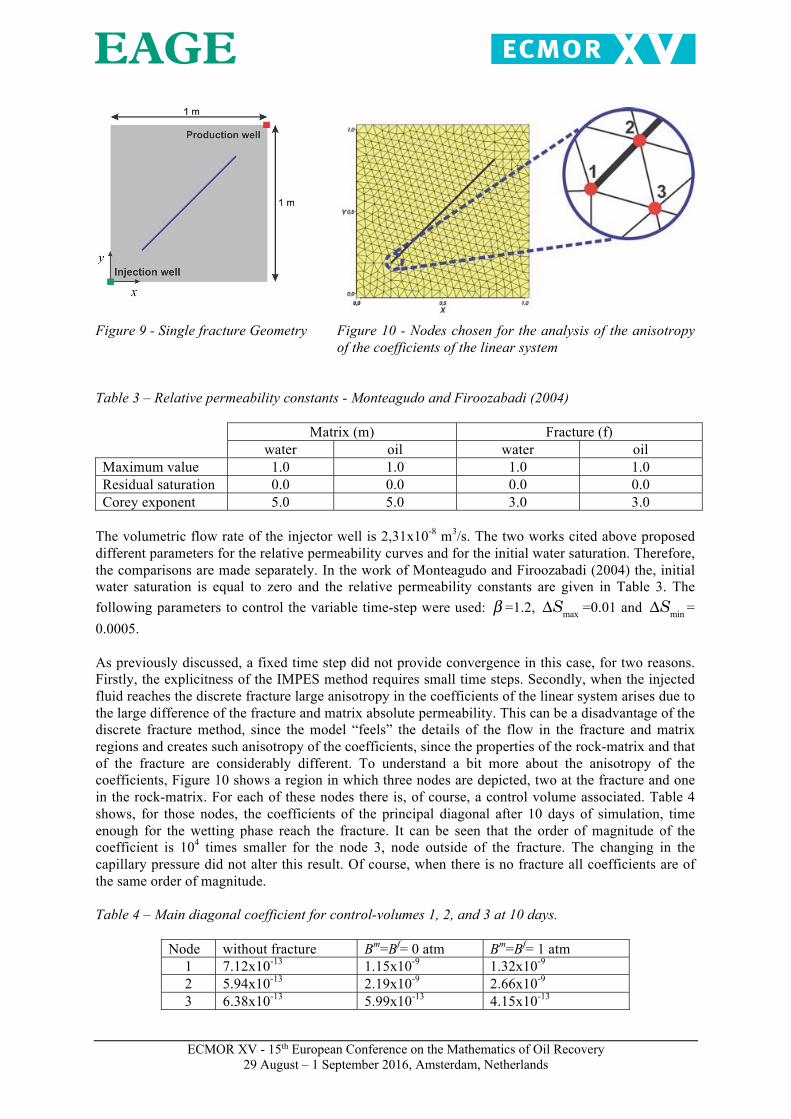
ΔSmin , the results are accepted and the time step is multiplied by the same factorβ . Following, results demonstrating the applicability of the method for several case studies are presented. Results Validation The main goal of this work is to advance a numerical scheme using EbFVM to deal with discrete fractures in conjunction with the superposition principle. Therefore, it does not addresses the complexity of modelling real fractured reservoirs, but deals with details of the numerical technology employed. Mostly of the results for natural fractured reservoirs available in the literature are presented in terms of saturation fields, which gives only quantitative behaviour of the problem. Checking the oil production permits to evaluate the performance of the method, and how well the connections between the rock-matrix and fractures are numerically handled. In this paper, the numerical works of Monteagudo and Firoozabadi (2004) and Marcondes et al. (2010) are employed for validation purposes. Test Case 1 - Single fracture in a quarter of five-spot configuration The validation tests start with a single fracture located in a quarter-of-five spot configuration with an injector well in the left-bottom corner and a production well at the right-upper-right corner, as shown in Figure 9. The thickness of the fracture is 10-4 m and the fluid and rock properties are given in Tables 1 and 2. Table 1 – Fluid properties Wetting phase Non-wetting phase Viscosity, Pa.s 0.8x10-3 0.45x10-3

Table 2 – Porous media properties Matrix Fracture Porosity 0.2 1.0 Permeability , m2 9.87x10-16 8.26x10-10



Figure 9 - Single fracture Geometry Figure 10 - Nodes chosen for the analysis of the anisotropy of the coefficients of the linear system

Table 3 – Relative permeability constants - Monteagudo and Firoozabadi (2004) Matrix (m) Fracture (f) water oil water oil Maximum value 1.0 1.0 1.0 1.0 Residual saturation 0.0 0.0 0.0 0.0 Corey exponent 5.0 5.0 3.0 3.0

The volumetric flow rate of the injector well is 2,31x10-8 m3/s. The two works cited above proposed different parameters for the relative permeability curves and for the initial water saturation. Therefore, the comparisons are made separately. In the work of Monteagudo and Firoozabadi (2004) the, initial water saturation is equal to zero and the relative permeability constants are given in Table 3. The following parameters to control the variable time-step were used: β =1.2, ΔSmax =0.01 and ΔSmin = 0.0005. As previously discussed, a fixed time step did not provide convergence in this case, for two reasons. Firstly, the explicitness of the IMPES method requires small time steps. Secondly, when the injected fluid reaches the discrete fracture large anisotropy in the coefficients of the linear system arises due to the large difference of the fracture and matrix absolute permeability. This can be a disadvantage of the discrete fracture method, since the model “feels” the details of the flow in the fracture and matrix regions and creates such anisotropy of the coefficients, since the properties of the rock-matrix and that of the fracture are considerably different. To understand a bit more about the anisotropy of the coefficients, Figure 10 shows a region in which three nodes are depicted, two at the fracture and one in the rock-matrix. For each of these nodes there is, of course, a control volume associated. Table 4 shows, for those nodes, the coefficients of the principal diagonal after 10 days of simulation, time enough for the wetting phase reach the fracture. It can be seen that the order of magnitude of the coefficient is 104 times smaller for the node 3, node outside of the fracture. The changing in the capillary pressure did not alter this result. Of course, when there is no fracture all coefficients are of the same order of magnitude. Table 4 – Main diagonal coefficient for control-volumes 1, 2, and 3 at 10 days.

Node without fracture Bm=Bf= 0 atm Bm=Bf= 1 atm 1 7.12x10-13 1.15x10-9 1.32x10-9 2 5.94x10-13 2.19x10-9 2.66x10-9 3 6.38x10-13 5.99x10-13 4.15x10-13



Figure 11 shows the three triangular grids employed to perform the grid refinement study. The results obtained using these grids without capillary pressure are depicted in Figure 12, demonstrating that the finer grid used in all calculations (Fig. 11c) is fine enough for the purposes of this work.

Figure 11 - Grids employed for the grid refinement study

For this validation two values of capillary pressure parameters for the fracture (Bf) and one for the matrix (Bm) were used, B

m = 1atm . The obtained results are shown in Figure 12b.

(a)

(b)

Figure 12 – (a) Grid refinement study, (b) and numerical results compared with the results of Monteagudo and Firoozabadi (2004).

The results obtained in this work show a little higher oil production than the ones obtained by Monteagudo and Firoozabadi (2004), for both capillarity pressure values. The breakthrough (time for the injected flow to reach the production well) differs in about 2 days, representing 4% difference. Figure 13 compares the results without capillary pressure effect with the results of Marcondes et al. (2010). If one compares the results of Figures 12 and 13, one can see that the results are very similar.



Figure 13 – Comparison of the oil recovery with the one obtained by Marcondes et al. (2010) Figure 14 presents the saturation fields at 50 days after production for different values of capillary pressure. The results are similar to the ones presented by several other works and, clearly, demonstrated that the presence of the fracture accelerates the breakthrough, and the capillary pressure retards this event. Obviously, the later conclusion is dependent on the capillarity pressure data of the rock-matrix and fracture media. Therefore, an analysis can be done in terms of the relation B

m / Bf . For values of this ratio greater than 1.0, the water passage through the fractures are limited, therefore, increase the life span of the reservoir. From Figure 14, it can be seen that there is a degree of imbibition of the wetting phase, coming from the fracture.

Figure 14 - Saturation of the wetting phase at 50 days for different values of capillarity pressure

Test Case 2 – Geometry with 6 fractures The second test case was also presented by Marcondes et al. (2010), but now with 6 discrete fractures considered, as depicted in Figure 15. In this case only qualitative comparisons are made through the saturation fields. Figures 16 and 17 show the saturation fields at 25 days of production for different values of capillarity pressure, and without capillary pressure for three production times, respectively. For the case with no capillary pressure the iso-saturation lines are very similar to the work of Marcondes et al. (2010), as seen in Figure 17, but the oil recovered with the model of this paper is slightly higher since the breakthrough occurs early. This difference increases when the values of



B

m / Bf increases, and at the end of 100 days, the oil recovered is about 5% higher, as depicted in Figure 18.

Figure 15 - Region with multiples fractures

When the discrete fracture model is used, it means that one is interested in representing with fidelity the network of fractures. There is a price to pay for having the details of the fracture flow. Figure 19 shows a situation where the fractures intercept themselves. In this situation, not only the nodes need to be given to the algorithm, but also the connectivity among them, otherwise it could be considered that the path joining nodes 2 and 3 is part of a fracture. For a large field with many fractures, this may be computational expensive.



Figure 16 - Comparison of the saturation fields with the work of Marcondes et al (2010) after 25 days of simulation. a) Bm = Bf = 0 atm ,

b) Bm = Bf = 1 atm and

c) Bm = 1 atm and Bf = 0.2 atm

Figure 17 - Comparison with the work of Marcondes et al (2010) for B

m = Bf = 0 atm a) 12 days b) 25 days c) 40 days

Figure 18 – Oil recovered – Multiple fractures



Figure 19 – Nodes involved in a fracture intersection

Influences of the fracture properties on the flow The final part of this paper is dedicated to present some influences of the properties of the fractures on the flow. The discrete fracture model offers this possibility, since the details of the fractures network enters the model. The following tests uses the data employed for the case study 1, with a single fracture and without capillary pressure effect. The grid employed is the one shown in Figure 11 (b). Figure 20 shows the penetration of the injected fluid at 5, 10, 25, and 35 days. It can be seen that for 35 days the wetting fluid reaches the production well. If no fracture were present this time would be 68 days. The presence of the fracture, therefore, advances the breakthrough by almost half of the time.

Figure 20 - Influence of the discrete fracture on the flow

Starting with the data from Table 2, the permeability was decreased, and as well as increased, by 10 and 100 times. As shown in Fig. 21, for the two cases in which the permeability of the fracture



decreases, the arrival of the water at the producing well is retarded, since the fracture no longer offers an easy path for the flow. For the two cases in which the permeability increases, it was not noticed appreciable difference. It is speculated that the oil recovery remain almost the same because the matrix coefficients corresponding to the fracture are already larger than the rock matrix coefficients, and further increase in the permeability does not alter this situation. Figure 22 shows the saturation field for three different values of permeability of the fractures.

Figure 21 – Influence of the fracture permeability on the oil recovery

Figure 22 – Saturation fields at 50 days for different values of permeability, a)

Kf = 8.26x10−12 m2 , b) K

f = 8.26x10−11 m2, and c) Kf = 8.26x10−10 m2

Anisotropy of the rock matrix All tests up to this point were performed considering the rock matrix as isotropic in order to compare with available results from the literature. However, the model implemented in this work does not impose such a restriction, and, as example, Figure 23 shows the saturation fields at 50 days for the



Case 1 without considering the capillary pressure and changing the value of the Kxx component of the permeability tensor.

Figure 23 - Saturation fields at 50 days for anisotropic permeability tensor of the rock matrix a)

Kxx = K yy , b)

Kxx = 2K yy and c) Kxx = 4K yy

Conclusions This paper addresses a numerical method for solving multiphase fluid flows in naturally fractured reservoirs using the discrete fracture method in conjunction with the Element based Finite-Volume method. Even being the fracture network in a real reservoir extremely complex, which still precludes the ample use of the discrete fracture approach, efforts need to be done in order to understand and apply the numerical technologies to calculate the complex flow among rock-matrix and fracture media. In this paper, we addressed this topic using a conservative multi-point flux approximation for the unknowns of fracture and matrix. Although the investigation has been performed for 2D fractured reservoirs, it was possible to demonstrate that the EbFVM is a viable alternative for discretizing the conservation equations of the fracture and matrix media. The linkage between rock and matrix is naturally handled due to the conservative approach of the method, and the contribution of the fractures is naturally added to the fluxes of the matrix. Results are presented for several cases in terms of oil production and water saturation fields. From the outcome of the numerical tests, one can state that the treatment of the anisotropy of the matrix coefficients, which creates difficulties for the solution of the linear system, is still an open issue. References Barenblatt, G. E., Zheltov, I. P. and Kochina, I. N. [1960] Basic concepts in the theory of seepage of homogeneous liquids in fissured rocks strata, PMM (Soviet Applied Mathematics and Mechanics), v. 24, n. 5, pp. 852– 864.

Baca, R. G., Arnett, R. C. and Langford, D. W. [1984] Modelling fluid flow in fractured-porous rock masses by finite-element techniques. International Journal for Numerical Methods in Fluids, v. 4, n. 4, pp. 337–348.

Baliga, B.R. and Patankar, S.V. [1983] A control volume finite-volume method for two-dimensional fluid flow and heat transfer Numerical Heat Transfer, v. 6, n. 3, pp. 245-261.

Benedetto M.F., Berrone S., Pieraccini S. and Scialò S. [2014] The virtual element method for



discrete fracture network simulations. Computer Methods in Applied Mechanics and Engineering, 2014, vol. 280 n. 1, pp. 135-156.

Blaskovich, F. T., Cain, G. M., Sonier, F., Waldren, D.; and Webb, S. J. [1983]. A multicomponent isothermal system for efficient reservoir simulation. In: Middle East Oil Technical Conference and Exhibition. Cordazzo, J. Maliska, C.R. Silva, A. F. C. and Hurtado, F. S. V. [2005] An element based conservative scheme using unstructured grids for reservoir simulation. In: 18th World Petroleum Congress, Johannesburg, South Africa. Corey, A. T. [1954] The Interrelation Between Gas and Oil Relative Permeabilities. Production Monthly, v. 19, pp. 38–41.

Dogru, A. H., Dreiman, W. T., Hemanthkumar, K. and Fung, L. S. [2001] Simulation of super-k behavior in ghawar by a multi-million cell parallel simulator. In: Proceedings of the SPE Middle East Oil Technical COnference and Exhibition, Bahrain.

Gong, B. Effective Models of Fractured Systems. [2007] Ph.D. Dissertation, Stanford University.

Haegland, H., Assteerawatt, A., Dahle, H.K., Eigestad G.T. and Helmig, R. [2009] Comparison of a cell-and vertexcentered discretization methods for flow in a two-dimensional discrete fracture-matrix system, Advances in Water Resources, vol.32, issue 12.

Hsieh, P. A. and Neumann, S. P. [1985] Field Determination of the Three- Dimensional Hydraulic Conductivity Tensor of Anisotropic Media: 1. Theory. Water Resources Research, v. 21, n. 11, pp. 1655–1665.

Hill, A. and Thomas, G. [1985] A new approach for simulating complex fractured reservoirs. In: Middle East Oil Technical Conference and Exhibition. Hirasaki, G. and Zhang, D. L. [2004] Surface Chemistry of Oil Recovery From Fractured, Oil-Wet, Carbonate Formations, Society of Petroleum Engineers, v. 9, pp. 151–162.

Horie, T., Firoozabadi, A. and Ishimito, K. [1990] Laboratory studies of capillary interaction in fracture/matrix systems, SPE Reservoir Eval. Eng., v. 5, pp. 353–360.

Hurtado, F.S.V., Maliska, C.R., Silva, A.F.C. and Cordazzo, J. [2007]. A quadrilateral element-based finite-volume formulation for the simulation of complex reservoirs, Proceedings of the X Latin American and Caribbean Petroleum Engineering Conference, LACPEC, Buenos Aires, Argentina.

Kaul , S. P., Putra, E. and Schechter, D. S. [2004] Simulation of spontaneous imbibition using Rayleigh-Ritz finite element method – a discrete fracture approach. In: Canadian International Petroleum Conference. Petroleum Society of Canada.

Karimi-Fard, M. and Firoozabadi, A. [2001]. Numerical simulation of water injection in 2d fractured media using discrete-fracture model. In: SPE Annual Technical Conference and Exhibition, vol. 6, p. 117 – 126, New Orleans, Louisiana. Society of Petroleum Engineers

Kazemi, H., Merrill Jr., L. S., Porterfield, K. L. and Zeman, P. R. [1976] Numerical simulation of water-oil flow in naturally fractured reservoirs. SPE Journal, v. 16, n. 06, pp. 317–326.



Kim, J.; Deo, M. [2000] Finite element, discrete fracture model for multiphase flow in porous media. AIChE Journal, v. 46, n. 6, p. 1120–1130.

La pointe, P. R., Eiben, T. and Dershowitz, W. [1997] Compartmen- talization analysis using discrete fracture network models. In: 4th International Reservoir Characterization Technical Conference, Houston, TX.

Lee, S.H., Lough, M. F. and Jensen, C. L. [2001] Hierarchical modeling of flow in naturally fractured formations with multiple length scales. Water Resources Research, v. 37, pp. 443–455.

Li, L. and Lee, S. H. [2008] Efficient Field-Scale Simulation of Black Oil in a Naturally Fractured Reservoir Through Discrete Fracture Networks and Homogenized Media. SPE Reservoir Evaluation & Engineering, v. 11, pp. 750–758.

Long, J. C. S. and Witherspoon, P. A. [1985] The relationship of the degree of interconnection to permeability in fracture networks. Journal of Geophysical Research: Solid Earth, v. 90, n. B4, pp. 3087–3098.

Marcondes, F. Varavei, A. Sepehrnoori, K. [2010] An element-based finite-volume method approach for naturally fractured compositional reservoir simulation. In: 13th Brazilian Congress of Thermal Sciences and Engineering.

Matthai, S.M., Mezentsev, A. and Belayneh, M. [2007] Finite Element-Node Centered Finite-Volume Two Phase Flow Experiments with Fractured Rock Represented by Unstructured Hybrid-Element Meshes. SPE Reservoir Simulation Symposium (SPE 93341), The Woodlands, Texas, January 31st.

Moinfar, A., Narr, W., Hui, M-H.; Mallison, B. T. and Lee, S. H. [2011] Comparison of discrete-fracture and dual-permeability models for multiphase flow in naturally fractured reservoirs. In: SPE Reservoir Simulation Symposium, The Woodlands, Texas, USA

Moinfar, A., VARAVEI, A., SEPEHRNOORI, K. and Johns, R. T. [2012] Development of a novel and computationally efficient discrete-fracture model to study ior processes in naturally fractured reservoirs. In: SPE Improved Oil Recovery Symposium. Society of Petroleum Engineers

Monteagudo, J. E. P. and Firoozabadi A. [2004] Control-volume method for numerical simulation of two-phase immiscible flow in two- and three-dimensional discrete-fractured media. Water Resources Rese- arch, v. 40, pp. 1–20.

Naimi-Tajdar, R. [2005] Development and implementation of a naturally fractured reservoir model into a fully implicit, equation-of-state compositional, parallel simulator. Ph.D. Dissertation, University of Texas at Austin.

Neuman, S. P. [1988] Stochastic Continuum Representation of Fractured Rock Permeabilityas an Alternative to the REV and Fracture Network Concepts. In: Custodio, E.; Gurgui, A.; Ferreira, J. (eds.). Groundwater Flow and Quality Modelling, vol. 224 of NATO ASI Series, pp. 331–362. Springer Netherlands.

Noorishad, J. and Mehran, M. [1982] An upstream finite element method for solution of transient transport equation in fractured porous media. Water Resources Research, v. 18, n. 3, pp. 588–596.

Peaceman, D. W. [1978] Interpretation of Well-Block Pressures in Numerical Reservoir Simulation.



Society of Petroleum Engineers Journal, v. 18, pp. 183 – 194, 1978.

Phelps, R., Pham, T. and Shari, A.M. [2000] Rigorous inclusion of faults and fractures in 3-D simulation. In: Proceedings of the SPE Asia Pacific Conference on Integrated Modeling for Asset Management, Yokohoma, Japan.

Pooladi-Darvish, M. and Firoozabadi, A. [2000] Experiments and modeling of water injection in water-wet fractured porous media. Petroleum Society of Canada, v. 39, Brasília, DF, pp. 31–42.

Raw, M.J. [1986] A New Control-Volume-Based Finite Element Procedure for the Numerical Solution of the Fluid Flow and Scalar Transport Equations. Ph.D. Dissertation, University of Waterloo, Waterloo, Ontario, Canada. Rhie, C.M. and Chow, W.L. [1983] Numerical Study of the Turbulent Flow Past an Airfoil with Trailing Edge Separation”. American Institute of Aeronautics and Astronautics Journal, Volume 21, Number 11, Pages 1525–1532. Rosa, A. J., Carvalho, R. D. S. and Xavier, J. A. D. [2006] Engenharia De Reservatórios De Petróleo, Editora Interciência, Rio de Janeiro, in Portuguese.

Schneider, G.E., Raw, M.J. [1986] A Skewed, Positive Influence Coefficient Upwinding Procedure for Control-Volume-Based Finite Element Convection-Diffusio Computation, Numerical Heat Transfer, Volume 8, Pages 1–26. Thomas, J. E. [2001] Fundamentos de Engenharia de Petróleo. Editora Interciência, Rio de Janeiro.

Thomas, L.K., Dixon, T.N. and Pierson, R.G. [1983] Fractured Reservoir Simulation. Soc. Petrol. Eng., v. 23, pp. 42-54.

Van Lingen, P., Sengul, M., Daniel, J.M. and Cosentino, L. [2001] Single medium simulation of fractured reservoirs with conductive faults and fractures. In: Proceedings of the SPE Middle East Oil Technical Conference and Exhibition, Bahrain.

Warren, J. E. and Root, P. J. The behavior of naturally fractured reservoirs. [1963] Soc. Petrol. Eng. J., v. 3, pp. 245–255.

Documents

Discrete Fracture Method for Petroleum Reservoir ... · Discrete Fracture Method for Petroleum Reservoir Simulation Using an Element-based Finite Volume Method C.R. Maliska* (Federal