DISCRETE GEODESIC CALCULUS IN THE SPACE …numod.ins.uni-bonn.de/research/papers/public/RuWi12.pdfGeodesic paths in shape space allow to ... path establishes correspondences between

DISCRETE GEODESIC CALCULUS IN THE SPACE OF VISCOUS FLUIDICOBJECTS

MARTIN RUMPF∗ AND BENEDIKT WIRTH†

Abstract. Based on a local approximation of the Riemannian distance on a manifold by a computationallycheap dissimilarity measure, a time discrete geodesic calculus is developed, and applications to shape space areexplored. The dissimilarity measure is derived from a deformation energy whose Hessian reproduces the underlyingRiemannian metric, and it is used to define length and energy of discrete paths in shape space. The notion of discretegeodesics defined as energy minimizing paths gives rise to a discrete logarithmic map, a variational definition of adiscrete exponential map, and a time discrete parallel transport. This new concept is applied to a shape space in whichshapes are considered as boundary contours of physical objects consisting of viscous material. The flexibility andcomputational efficiency of the approach is demonstrated for topology preserving shape morphing, the representationof paths in shape space via local shape variations as path generators, shape extrapolation via discrete geodesic flow,and the transfer of geometric features.

Key words. Shape space, geodesic paths, exponential map, logarithm, parallel transport

AMS subject classifications. 68U10, 53C22, 74B20, 49M20

1. Introduction. Geodesic paths in shape space allow to define smooth and in somesense geometrically or physically natural connecting paths O(t), t ∈ [0, 1], between twogiven shapesO(0),O(1), or they enable the extrapolation of a path from an initial shapeO(0)and an initial shape variation δO which encodes the path direction. Applications includeshape modeling in computer vision [17, 16], computational anatomy, where the morphingpath establishes correspondences between a patient and a template [2, 26], shape clusteringbased on Riemannian distances [32], as well as shape statistics [9, 13], where geodesic pathsin shape space transport information from the observed shapes into a common reference framein which statistics can be performed.

As locally length minimizing paths, geodesic paths require to endow the space of shapeswith a Riemannian metric which encodes the preferred shape variations. There is a richdiversity of Riemannian shape spaces in the literature. Kilian et al. compute isometry invari-ant geodesics between consistently triangulated surfaces [16], where the Riemannian metricmeasures stretching of triangle edges, while the metric by Liu et al. also takes into accountdirectional changes of edges [22].

For planar curves, different Riemannian metrics have been devised, including the L2-metric on direction and curvature functions [17], the L2-metric on stretching and bendingvariations [31], as well as curvature-weighted L2- or Sobolev-type metrics [25, 34], some ofwhich allow closed-form geodesics [37, 33]. A variational approach to the computation ofgeodesics in the space of planar Jordan curves has been proposed by Schmidt et al. in [30].The extrapolation of geodesics in the space of curves incorporating translational, rotational,and scale invariance has been investigated by Mennucci et al. [24]. A Riemannian space ofnon-planar elastic curves has very recently been proposed by Srivastava et al. [32].

In the above approaches, the shape space is often identified with a so-called pre-shapespace of curve parameterizations over a 1D domain (or special representations thereof) mod-ulo the action of the reparameterization group. It is essential that the metric on the pre-shapespace is invariant under reparameterization or equivalently that reparameterization representsan isometry in the pre-shape space so that the Riemannian metric can be inherited by the

∗Bonn University, Endenicher Allee 60, D-53115 Bonn, Germany ([email protected]).†Courant Institute, New York University, 251 Mercer Street, New York, NY 10012, USA

([email protected]).

1

2 MARTIN RUMPF AND BENEDIKT WIRTH

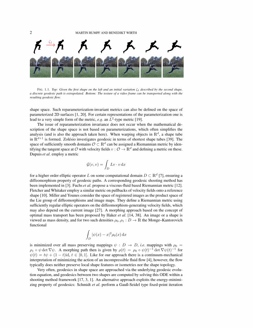
ζ1−→

FIG. 1.1. Top: Given the first shape on the left and an initial variation ζ1 described by the second shape,a discrete geodesic path is extrapolated. Bottom: The texture of a video frame can be transported along with theresulting geodesic flow.

shape space. Such reparameterization-invariant metrics can also be defined on the space ofparameterized 2D surfaces [1, 20]. For certain representations of the parameterization one islead to a very simple form of the metric, e.g. an L2-type metric [19].

The issue of reparameterization invariance does not occur when the mathematical de-scription of the shape space is not based on parameterizations, which often simplifies theanalysis (and is also the approach taken here). When warping objects in Rd, a shape tubein Rd+1 is formed. Zolesio investigates geodesic in terms of shortest shape tubes [39]. Thespace of sufficiently smooth domainsO ⊂ Rd can be assigned a Riemannian metric by iden-tifying the tangent space atO with velocity fields v : O → Rd and defining a metric on these.Dupuis et al. employ a metric

G(v, v) =

∫D

Lv · v dx

for a higher order elliptic operator L on some computational domain D ⊂ Rd [7], ensuring adiffeomorphism property of geodesic paths. A corresponding geodesic shooting method hasbeen implemented in [3]. Fuchs et al. propose a viscous-fluid based Riemannian metric [12].Fletcher and Whitaker employ a similar metric on pullbacks of velocity fields onto a referenceshape [10]. Miller and Younes consider the space of registered images as the product space ofthe Lie group of diffeomorphisms and image maps. They define a Riemannian metric usingsufficiently regular elliptic operators on the diffeomorphism-generating velocity fields, whichmay also depend on the current image [27]. A morphing approach based on the concept ofoptimal mass transport has been proposed by Haker et al. [14, 38]. An image or a shape isviewed as mass density, and for two such densities ρ0, ρ1 : D → R the Monge–Kantorovichfunctional ∫

D

|ψ(x)− x|2ρ0(x) dx

is minimized over all mass preserving mappings ψ : D → D, i.e. mappings with ρ0 =ρ1 ◦ ψ det∇ψ. A morphing path then is given by ρ(t) = ρ0 ◦ ψ(t)−1 det∇ψ(t)−1 forψ(t) = tψ + (1 − t)id, t ∈ [0, 1]. Like for our approach there is a continuum-mechanicalinterpretation of minimizing the action of an incompressible fluid flow [4], however, the flowtypically does neither preserve local shape features or isometries nor the shape topology.

Very often, geodesics in shape space are approached via the underlying geodesic evolu-tion equation, and geodesics between two shapes are computed by solving this ODE within ashooting method framework [17, 3, 1]. An alternative approach exploits the energy-minimi-zing property of geodesics: Schmidt et al. perform a Gauß-Seidel type fixed-point iteration

DISCRETE GEODESIC CALCULUS IN THE SPACE OF VISCOUS FLUIDIC OBJECTS 3

which can be interpreted as a gradient descent on the path energy, and Srivastava et al. de-rive the equations of a gradient flow for the path energy which they then discretize [32]. Incontrast, we employ an inherently variational formulation where geodesics are defined asminimizers of a time discrete path energy. Discrete geodesics are then defined consistently asminimizers of a corresponding discrete energy.

In this paper we start from this time discretization and consistently develop a time dis-crete geodesic calculus in shape space. The resulting variational discretization of the basicRiemannian calculus consists of an exponential map, a logarithmic map, parallel transport,and finally an underlying discrete connection. To this end, we replace the exact, computation-ally expensive Riemannian distance by a relatively cheap but consistent dissimilarity measure.Our choice of the dissimilarity measure not only ensures consistency for vanishing time stepsize but also a good representation of shape space geometry already for coarse time steps.For example, rigid body motion invariance is naturally incorporated in this approach. Weillustrate this approach on a shape space consisting of homeomorphic viscous-fluid objectsand a corresponding deformation-based dissimilarity measure.

Different from most approaches, which first discretize in space via the choice of a param-eterization, a set of control points, or a mesh, and then solve the resulting transport equationsby suitable solvers for ordinary differential equations (see the discussion above), our timediscretization is defined on the usually infinite dimensional shape space. It results from aconsistent transfer of time continuous to time discrete variational principles. Thereby, it leadsto a collection of variational problems on the shape space, which in our concrete implemen-tation of the proposed calculus consists of non-parameterized, volumetric objects.

Let us also already mention a further remarkable conceptual difference. The way the timediscrete geodesic calculus is introduced differs substantially from the way the time continuouscounterpart is usually developed. In classical Riemannian differential geometry one firstdefines a connection (v, w) 7→ ∇vw for two vector fields v and w on a manifoldM. Withthe connection at hand a tangent vectorw can be transported parallel along a path with motionfield v solving ∇vw = 0. Studying those paths where the motion field itself is transportedparallel along the path (i.e. it solves the ODE ∇vv = 0) one is led to geodesics. Next, theexponential map is introduced via the solution of the above ODE for varying initial velocity.Finally, the logarithm is obtained as the (local) inverse of the exponential map.

In the time discrete calculus we start with a time discrete formulation of path length andenergy and then define discrete geodesics as minimizers of the discrete energy. Evaluatingthe initial step of a discrete geodesic path as the discrete counterpart of the initial velocity weare led to the discrete logarithm. Then, the discrete exponential map is defined as the inverseof the discrete logarithm. Next, discrete logarithm and discrete exponential allow to define adiscrete parallel transport based on the construction of a sequence of approximate Riemannianparallelograms (commonly known as Schild’s ladder [8]). Finally, with the discrete paralleltransport at hand, a time discrete connection can be defined.

Let us note that the approximation of parallel transport in shape space via Schild’s ladderhas also been used in the context of the earlier mentioned flow of diffeomorphism approach[29, 23]. In our discrete framework, however, the notion of discrete parallel transport isdirectly derived from the parallelogram construction, consistently with the overall discreteapproach to geodesics.

A related approach for time discrete geodesics has been presented in an earlier paper byWirth et al. [36]. In contrast to [36], we here do not restrict ourselves to the computationof geodesic paths between two shapes but devise a full-fledged theory of discrete geodesiccalculus (cf . Figure 1). Furthermore, different from that approach we ensure topological con-sistency and describe shapes solely via deformations of reference objects instead of treating


deformations and level set representations of shapes simultaneously as degrees of freedom,which in turn strongly simplifies the minimization procedure.

The paper is organized as follows. In Section 2 we introduce a special model for a shapespace, the space of viscous fluidic objects, to which we restrict our exposition of the geodesiccalculus. Here, in the light of the discrete shape calculus to be developed, we will review thenotion of discrete path length and discrete path energy. After these preliminaries the actualtime discrete calculus consisting of a discrete logarithm, a discrete exponential and a discreteparallel transport together with a discrete connection is introduced and discussed in Section3. Then, Section 4 is devoted to the numerical discretization via characteristic functions anda parameterization via deformations over reference paths. Finally, we draw conclusions inSection 5.

2. A space of volumetric objects and an elastic dissimilarity measure. To keep theexposition focused we restrict ourselves to a specific shape model, where shapes are repre-sented by volumetric objects which behave physically like viscous fluids. In fact, the scopeof the variational discrete geodesic calculus extends beyond this concrete shape model. Werefer to Section 5 for remarks on the application to more general shape spaces.

2.1. The space of viscous-fluid objects. Let us introduce the spaceM of shapes as theset of all objects O which are closed subsets of Rd (d = 2, 3) and homeomorphic to a givenregular reference object Oref, i.e. O = φ(Oref) for an orientation preserving homeomorphismφ. Furthermore, objects which coincide up to a rigid body motion are identified with eachother. A smooth path (O(t))t∈[0,1] in this shape space is associated with a smooth family(φ(t))t∈[0,1] of deformations. To measure the distance between two objects, a Riemannianmetric is defined on variations δO of objects O ∈M which reflects the internal fluid friction— called dissipation — that occurs during the shape variation. The local temporal rate ofdissipation in a fluid depends on the symmetric part ε[v] := 1

2 (∇v +∇vT ) of the gradient ofthe fluid velocity v : O → Rd (the antisymmetric remainder reflects infinitesimal rotations),and for an isotropic Newtonian fluid, we obtain the local rate of dissipation

diss(∇v) = λ(trε[v])2 + 2µtr(ε[v]2) , (2.1)

where λ, µ are material-specific parameters. Given a family (φ(t))t∈[0,1] of deformations ofthe reference objectOref, the change of shape along the path (O(t))t∈[0,1] can be described bythe (Lagrangian) temporal variation φ(t) or the associated (Eulerian) velocity field

v(t) = φ(t) ◦ φ−1(t)

on O. Hence, the tangent space TOM toM at a shape O can be identified with the spaceof initial velocities v = φ(0) ◦ φ−1(0) for deformation paths with φ(0,Oref) = O. Here weidentify those velocities v which lead to the same effective shape variation, i.e. those with thesame normal component v · n on ∂O, where n is the outer normal on ∂O. Now, integratingthe local rate of dissipation for velocity fields v on O = φ(0,Oref), we define the Riemannianmetric GO on TOM as the symmetric quadratic form with

GO(v, v) = min{v | v·n=v·n on ∂O}

∫Odiss(∇v(x)) dx . (2.2)

For the shape variation along a path O : [0, 1] →M described by the Eulerian motion field(v(t))t∈[0,1], path length L and energy E are defined as

L[(O(t))t∈[0,1]] =∫ 1

0

√GO(t)(v(t), v(t)) dt , (2.3)

E[(O(t))t∈[0,1]] =∫ 1

0GO(t)(v(t), v(t)) dt . (2.4)


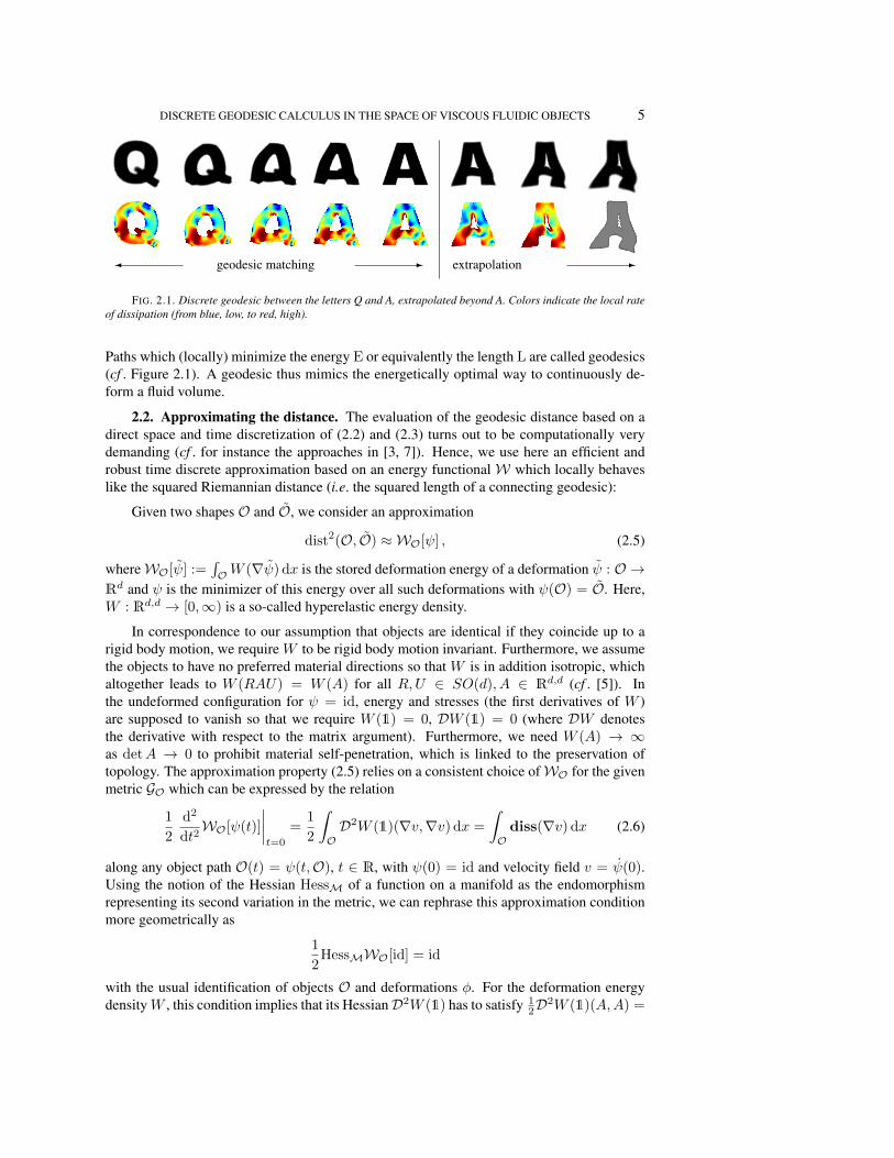
geodesic matching extrapolation� - -

FIG. 2.1. Discrete geodesic between the letters Q and A, extrapolated beyond A. Colors indicate the local rateof dissipation (from blue, low, to red, high).

Paths which (locally) minimize the energy E or equivalently the length L are called geodesics(cf . Figure 2.1). A geodesic thus mimics the energetically optimal way to continuously de-form a fluid volume.

2.2. Approximating the distance. The evaluation of the geodesic distance based on adirect space and time discretization of (2.2) and (2.3) turns out to be computationally verydemanding (cf . for instance the approaches in [3, 7]). Hence, we use here an efficient androbust time discrete approximation based on an energy functionalW which locally behaveslike the squared Riemannian distance (i.e. the squared length of a connecting geodesic):

Given two shapes O and O, we consider an approximation

dist2(O, O) ≈ WO[ψ] , (2.5)

whereWO[ψ] :=∫OW (∇ψ) dx is the stored deformation energy of a deformation ψ : O →

Rd and ψ is the minimizer of this energy over all such deformations with ψ(O) = O. Here,W : Rd,d → [0,∞) is a so-called hyperelastic energy density.

In correspondence to our assumption that objects are identical if they coincide up to arigid body motion, we require W to be rigid body motion invariant. Furthermore, we assumethe objects to have no preferred material directions so that W is in addition isotropic, whichaltogether leads to W (RAU) = W (A) for all R,U ∈ SO(d), A ∈ Rd,d (cf . [5]). Inthe undeformed configuration for ψ = id, energy and stresses (the first derivatives of W )are supposed to vanish so that we require W (1) = 0, DW (1) = 0 (where DW denotesthe derivative with respect to the matrix argument). Furthermore, we need W (A) → ∞as detA → 0 to prohibit material self-penetration, which is linked to the preservation oftopology. The approximation property (2.5) relies on a consistent choice ofWO for the givenmetric GO which can be expressed by the relation

1

2

d2

dt2WO[ψ(t)]

∣∣∣∣t=0

=1

2

∫OD2W (1)(∇v,∇v) dx =

∫Odiss(∇v) dx (2.6)

along any object path O(t) = ψ(t,O), t ∈ R, with ψ(0) = id and velocity field v = ψ(0).Using the notion of the Hessian HessM of a function on a manifold as the endomorphismrepresenting its second variation in the metric, we can rephrase this approximation conditionmore geometrically as

1

2HessMWO[id] = id

with the usual identification of objects O and deformations φ. For the deformation energydensityW , this condition implies that its HessianD2W (1) has to satisfy 1

2D2W (1)(A,A) =


diss(A) for all A ∈ Rd,d . A suitable example is

W (A) =µ

2tr(ATA) +

λ

4detA2 −

(µ+

λ

2

)log detA− dµ

2− λ

4.

Assume that the energy density satisfies the above-mentioned properties. We observe that themetric GO is the first non-vanishing term in the Taylor expansion of the squared length of acurve, i.e. (

L[(O(t))t∈[0,T ]])2

= T 2GO(0)(v, v) +O(T 3)

with v = φ(0) ◦ φ−1(0) being the initial tangent vector along a smooth path (O(t))t∈[0,T ] =(φ(t,Oref))t∈[0,1]. Thus, since the Hessian of the energyWO and the metric GO are related by(2.6), we obtain that the second order Taylor expansions of dist2(O, ψ(O)) andWO[ψ] in ψcoincide and indeed

dist2(O, O) = min{ψ |ψ(O)=O}

WO[ψ] +O(dist3(O, O)) . (2.7)

Here, different from [36] we neither take into account mismatch penalties nor perimeter reg-ularizing functionals for each object Ok, k = 0, . . . ,K.

2.3. Discrete length and discrete energy. Now, we are in a position to discretize lengthand energy of paths (O(t))t∈[0,1] in shape space. To this end, we first sample the path at timestk = kτ for k = 0, . . . ,K (τ = 1

K ), denote Ok := O(tk), and obtain the estimates

L[(O(t))t∈[0,1]] ≥∑Kk=1 dist(Ok−1,Ok)

E[(O(t))t∈[0,1]] ≥ 1τ

∑Kk=1 dist2(Ok−1,Ok)

for the length and the energy, where equality holds for geodesic paths. Indeed, the firstestimate is straightforward, and the application of the Cauchy–Schwarz inequality leads to

K∑k=1

dist2(Ok−1,Ok) ≤K∑k=1

(∫ kτ

(k−1)τ

√GO(t)(v(t), v(t)) dt

)2

≤K∑k=1

τ

∫ kτ

(k−1)τGO(t)(v(t), v(t)) dt = τ E[(O(t))t∈[0,1]]

which implies the second estimate.Together with (2.7) this motivates the following definition of a discrete path energy and

a discrete path length for a discrete path (O0, . . . ,OK) in shape space:

L[(O0, . . . ,OK)] =∑Kk=1

√WOk−1

[ψk] , (2.8)

E[(O0, . . . ,OK)] = 1τ

∑Kk=1WOk−1

[ψk] , (2.9)

where ψk = argmin{ψ |ψ(Ok−1)=Ok}WOk−1[ψ] (cf . also [36]). In fact, (2.8) and (2.9) can

for general smooth paths even be proven to be first order consistent with the continuouslength (2.3) and energy (2.4) as τ → 0. For illustration, ifM is a two-dimensional manifoldembedded in R3, we can interpret the termsWOk−1

as the stored elastic energies in springswhich connect a sequence of points Ok on the manifold through the ambient space. Then thediscrete path energy is the total stored elastic energy in this chain of springs.


��

CC

��

CC

��

CC

CC

��

CC

��

CC

��

CC

��

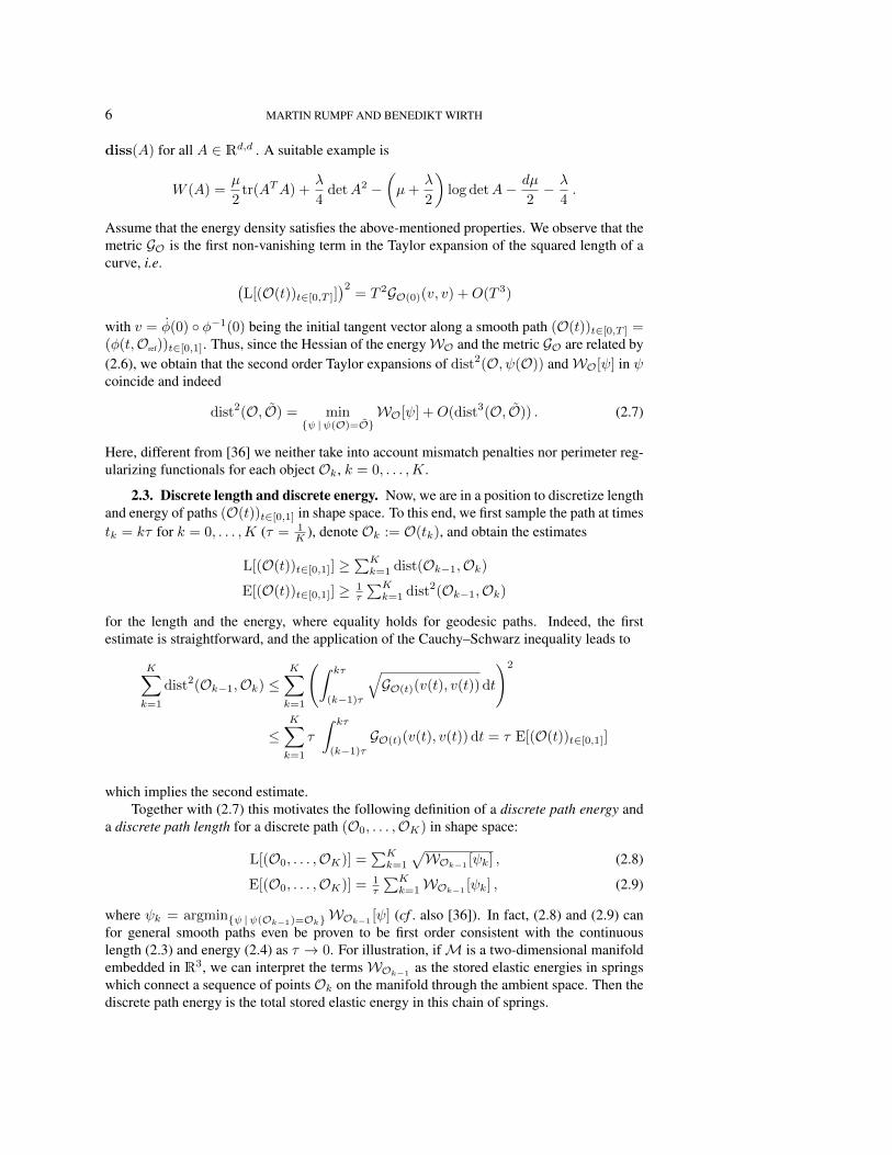
FIG. 2.2. Nonlinear video interpolation via a discrete geodesic (top) between two segmented photographs ofwhite and red blood cells (first and last picture of bottom row, courtesy Robert A. Freitas, Institute for MolecularManufacturing, California, USA). The bottom row shows pushforwards and pullbacks of the end images under thedeformations along the discrete geodesic.

A discrete geodesic (of order K) is now defined as a minimizer of E[(O0, . . . ,OK)] forfixed end points O0,OK . The discrete geodesic is thus an energetically optimal sequence ofdeformations from O0 into OK .

In the minimization algorithm to be discussed in Section 4.1 we do not explicitly mini-mize E[(O0, . . . ,OK)] for the object contours as in [36] but instead for reference deforma-tions defined on fixed reference objects. Figure 2.2 shows a discrete geodesic in the contextof multicomponent objects, which is visually identical to that obtained by the more com-plex approach in [36]. Here, deformations are considered which map every component of ashape onto the corresponding component of the next shape in the discrete path as the obviousgeneralization of discrete geodesics between single component shapes.

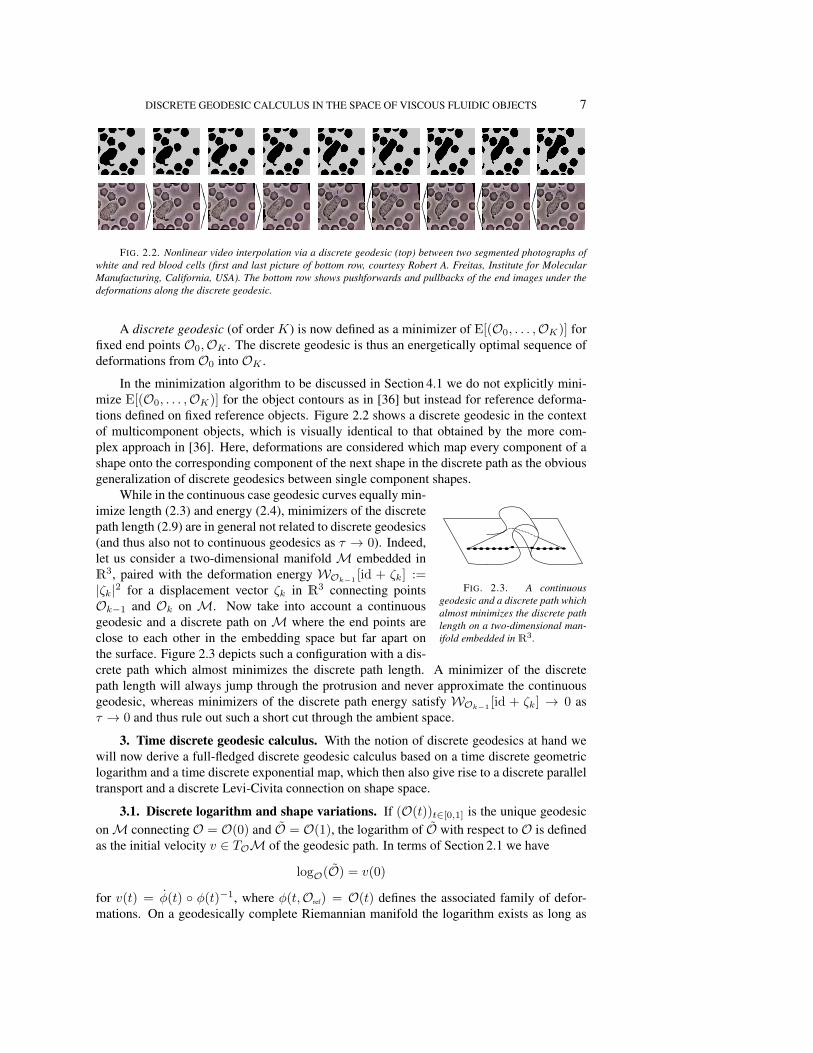
FIG. 2.3. A continuousgeodesic and a discrete path whichalmost minimizes the discrete pathlength on a two-dimensional man-ifold embedded inR3.

While in the continuous case geodesic curves equally min-imize length (2.3) and energy (2.4), minimizers of the discretepath length (2.9) are in general not related to discrete geodesics(and thus also not to continuous geodesics as τ → 0). Indeed,let us consider a two-dimensional manifold M embedded inR3, paired with the deformation energy WOk−1

[id + ζk] :=|ζk|2 for a displacement vector ζk in R3 connecting pointsOk−1 and Ok on M. Now take into account a continuousgeodesic and a discrete path on M where the end points areclose to each other in the embedding space but far apart onthe surface. Figure 2.3 depicts such a configuration with a dis-crete path which almost minimizes the discrete path length. A minimizer of the discretepath length will always jump through the protrusion and never approximate the continuousgeodesic, whereas minimizers of the discrete path energy satisfy WOk−1

[id + ζk] → 0 asτ → 0 and thus rule out such a short cut through the ambient space.

3. Time discrete geodesic calculus. With the notion of discrete geodesics at hand wewill now derive a full-fledged discrete geodesic calculus based on a time discrete geometriclogarithm and a time discrete exponential map, which then also give rise to a discrete paralleltransport and a discrete Levi-Civita connection on shape space.

3.1. Discrete logarithm and shape variations. If (O(t))t∈[0,1] is the unique geodesiconM connecting O = O(0) and O = O(1), the logarithm of O with respect to O is definedas the initial velocity v ∈ TOM of the geodesic path. In terms of Section 2.1 we have

logO(O) = v(0)

for v(t) = φ(t) ◦ φ(t)−1, where φ(t,Oref) = O(t) defines the associated family of defor-mations. On a geodesically complete Riemannian manifold the logarithm exists as long as


dist(O, O) is sufficiently small. The associated logarithmic map logO : O 7→ v(0) ∈ TOMrepresents (nonlinear) variations on the manifold as (linear) tangent vectors.

The initial velocity v(0) can be approximated by a difference quotient in time,

v(0, x) =1

τζ(x) +O(τ) ,

where ζ(x) = φ(τ, x) ◦ φ(0, x)−1 − x denotes a displacement on the initial object O. Thus,we obtain

τ logO(O) = ζ(x) +O(τ2) .

This gives rise to a consistent definition of a time discrete logarithm. Let (O0, . . . ,OK) be adiscrete geodesic between O = O0 and O = OK with an associated sequence of matchingdeformations ψ1, . . . , ψK , then we consider 1

τ ζ1 for the displacement ζ1(x) = ψ1(x)− x asan approximation of v(0) = logO(O). Taking into account that τ = 1

K we thus define thediscrete 1

K -logarithm

( 1KLOG)O(O) := ζ1 . (3.1)

In the special case K = 1 and a discrete geodesic (O, O) we simply obtain

( 11LOG)O(O) = argmin{ζ1 | (id+ζ1)(O)=O}WO[id + ζ1] .

As in the continuous case the discrete logarithm can be considered as a representation ofthe nonlinear variation O of O in the (linear) tangent space of displacements on O. On asequence of successively refined discrete geodesics we expect

K( 1KLOG)O(O)→ logO(O) (3.2)

for K →∞ (cf . Figure 3.1 for an experimental validation of this convergence behaviour).

3.2. Discrete exponential and shape extrapolation. In the continuous setting, the ex-ponential map expO maps tangent vectors v ∈ TOM onto the end point O(1) of a geodesic(O(t))t∈[0,1] with O(0) = O and the given tangent vector v at time 0. Using the notationfrom the previous section we have expO(v(0)) = O and, via a simple scaling argument,expO

(kK v(0)

)= O( kK ) for k = 0, . . . ,K. We now aim at defining a discrete power k

exponential map EXPkO such that EXPkO(ζ1) = Ok on a discrete geodesic (O,O1, . . . ,OK)of order K ≥ k with ζ1 = ( 1

KLOG)O(O) (the notation is motivated by the observation thatexp(ks) = expk(s) on R or more general matrix groups). Our definition will reflect thefollowing recursive properties of the continuous exponential map,

expO(1v) =(11 logO

)−1(v) ,

expO(2v) =(12 logO

)−1(v) ,

expO(kv) = expexpO((k−2)v)(2vk−1)

for vk−1 := logexpO((k−2)v) expO((k − 1)v) .

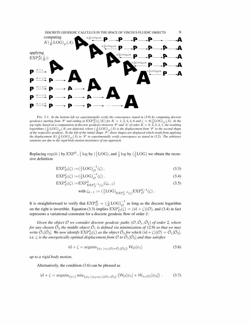
DISCRETE GEODESIC CALCULUS IN THE SPACE OF VISCOUS FLUIDIC OBJECTS 9computingK( 1

KLOG)P

(A):

-�1(1

1LOG)P(A)

--�2(1

2LOG)P(A)

---�3(1

3LOG)P(A)

----�4(1

4LOG)P(A)

-----�8(1

8LOG)P(A)

. . .

applyingEXPKP( ζK ):

-id + ζ

- -id + ζ/2

- - -id + ζ/3

- - - -id + ζ/4

- - - - -id + ζ/8 . . .

FIG. 3.1. In the bottom left we experimentally verify the convergence stated in (3.9) by computing discretegeodesics starting from ‘P’ and ending at EXPKP (ζ/K) for K = 1, 2, 3, 4, 8 and ζ = 8( 1

8LOG)

P(A). In the

top right, based on a computation of discrete geodesics between ‘P’ and ‘A’ of order K = 8, 4, 3, 2, 1, the resultinglogarithms ( 1

KLOG)

P(A) are depicted, where ( 1

KLOG)

P(A) is the displacement from ‘P’ to the second shape

of the respective geodesic. To the left of the initial shape ‘P’, those shapes are displayed which result from applyingthe displacement K( 1

KLOG)

P(A) to ‘P’ to experimentally verify convergence as stated in (3.2). The arbitrary

rotations are due to the rigid body motion invariance of our approach.

Replacing exp(k·) by EXPk, 11 log by ( 1

1LOG), and 12 log by ( 1

2LOG) we obtain the recur-sive definition

EXP1O(ζ) :=( 1

1LOG)−1O (ζ) , (3.3)

EXP2O(ζ) :=( 1

2LOG)−1O (ζ) , (3.4)

EXPkO(ζ) :=EXP2EXPk−2

O (ζ)(ζk−1) (3.5)

with ζk−1 := ( 11LOG)

EXPk−2O (ζ)

EXPk−1O (ζ) .

It is straightforward to verify that EXPKO = ( 1KLOG)

−1O as long as the discrete logarithm

on the right is invertible. Equation (3.3) implies EXP1O(ζ) = (id + ζ)(O), and (3.4) in fact

represents a variational constraint for a discrete geodesic flow of order 2 :

Given the object O we consider discrete geodesic paths (O, O1, O2) of order 2, wherefor any chosen O2 the middle object O1 is defined via minimization of (2.9) so that we maywrite O1[O2]. We now identify EXP2

O(ζ) as the object O2 for which (id + ζ)(O) = O1[O2],i.e. ζ is the energetically optimal displacement from O to O1[O2] and thus satisfies

id + ζ = argmin{ψ1 |ψ1(O)=O1[O2]}WO[ψ1] (3.6)

up to a rigid body motion.

Alternatively, the condition (3.6) can be phrased as

id + ζ = argmin{ψ1}min{ψ2 | (ψ2◦ψ1)(O)=O2}(WO[ψ1] +Wψ1(O)[ψ2]

). (3.7)


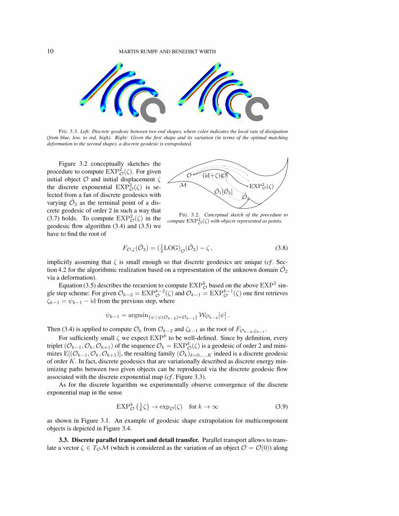
FIG. 3.3. Left: Discrete geodesic between two end shapes, where color indicates the local rate of dissipation(from blue, low, to red, high). Right: Given the first shape and its variation (in terms of the optimal matchingdeformation to the second shape), a discrete geodesic is extrapolated.

M(id+ζ)(O)O

EXP2O(ζ)

O2

O1[O2]

FIG. 3.2. Conceptual sketch of the procedure tocompute EXP2

O(ζ) with objects represented as points.

Figure 3.2 conceptually sketches theprocedure to compute EXP2

O(ζ). For giveninitial object O and initial displacement ζthe discrete exponential EXP2

O(ζ) is se-lected from a fan of discrete geodesics withvarying O2 as the terminal point of a dis-crete geodesic of order 2 in such a way that(3.7) holds. To compute EXP2

O(ζ) in thegeodesic flow algorithm (3.4) and (3.5) wehave to find the root of

FO,ζ(O2) = (12LOG)O(O2)− ζ , (3.8)

implicitly assuming that ζ is small enough so that discrete geodesics are unique (cf . Sec-tion 4.2 for the algorithmic realization based on a representation of the unknown domain O2

via a deformation).Equation (3.5) describes the recursion to compute EXPkO based on the above EXP2 sin-

gle step scheme: For givenOk−2 = EXPk−2O (ζ) andOk−1 = EXPk−1O (ζ) one first retrievesζk−1 = ψk−1 − id from the previous step, where

ψk−1 = argmin{ψ |ψ(Ok−2)=Ok−1}WOk−2[ψ] .

Then (3.4) is applied to compute Ok from Ok−2 and ζk−1 as the root of FOk−2,ζk−1.

For sufficiently small ζ we expect EXPk to be well-defined. Since by definition, everytriplet (Ok−1,Ok,Ok+1) of the sequenceOk = EXPkO(ζ) is a geodesic of order 2 and mini-mizes E[(Ok−1,Ok,Ok+1)], the resulting family (Ok)k=0,...,K indeed is a discrete geodesicof order K. In fact, discrete geodesics that are variationally described as discrete energy min-imizing paths between two given objects can be reproduced via the discrete geodesic flowassociated with the discrete exponential map (cf . Figure 3.3).

As for the discrete logarithm we experimentally observe convergence of the discreteexponential map in the sense

EXPkO(1k ζ)→ expO(ζ) for k →∞ (3.9)

as shown in Figure 3.1. An example of geodesic shape extrapolation for multicomponentobjects is depicted in Figure 3.4.

3.3. Discrete parallel transport and detail transfer. Parallel transport allows to trans-late a vector ζ ∈ TOM (which is considered as the variation of an object O = O(0)) along


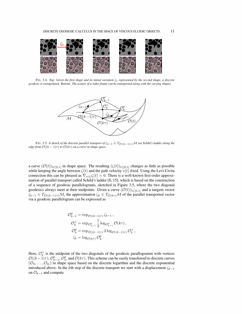
ζ1−→

FIG. 3.4. Top: Given the first shape and its initial variation ζ1 represented by the second shape, a discretegeodesic is extrapolated. Bottom: The texture of a video frame can be transported along with the varying shapes.

M O(t)O((k−1)τ)

O(kτ)

Opk−1

OpkO×k•

ζk−1

ζk•

•

•

•

FIG. 3.5. A sketch of the discrete parallel transport of ζk−1 ∈ TO((k−1)τ)M via Schild’s ladder along theedge fromO((k − 1)τ) toO(kτ) on a curve in shape space.

a curve (O(t))t∈[0,1] in shape space. The resulting (ζ(t))t∈[0,1] changes as little as possiblewhile keeping the angle between ζ(t) and the path velocity v(t) fixed. Using the Levi-Civitaconnection this can be phrased as ∇v(t)ζ(t) = 0. There is a well-known first-order approxi-mation of parallel transport called Schild’s ladder [8, 15], which is based on the constructionof a sequence of geodesic parallelograms, sketched in Figure 3.5, where the two diagonalgeodesics always meet at their midpoints. Given a curve (O(t))t∈[0,1] and a tangent vectorζk−1 ∈ TO((k−1)τ)M, the approximation ζk ∈ TO(kτ)M of the parallel transported vectorvia a geodesic parallelogram can be expressed as

Opk−1 = expO((k−1)τ) ζk−1 ,

O×k = expOpk−1

1

2logOpk−1

O(kτ) ,

Opk = expO((k−1)τ) 2 logO((k−1)τ)O×k ,ζk = logO(kτ)O

pk .

Here, O×k is the midpoint of the two diagonals of the geodesic parallogramm with verticesO((k−1)τ),Opk−1,Opk, andO(kτ). This scheme can be easily transferred to discrete curves(O0, . . . ,OK) in shape space based on the discrete logarithm and the discrete exponentialintroduced above. In the kth step of the discrete transport we start with a displacement ζk−1on Ok−1 and compute


ee

e e eee e

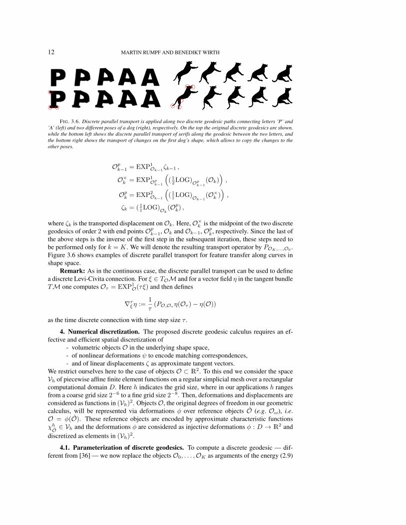
FIG. 3.6. Discrete parallel transport is applied along two discrete geodesic paths connecting letters ’P’ and’A’ (left) and two different poses of a dog (right), respectively. On the top the original discrete geodesics are shown,while the bottom left shows the discrete parallel transport of serifs along the geodesic between the two letters, andthe bottom right shows the transport of changes on the first dog’s shape, which allows to copy the changes to theother poses.

Opk−1 = EXP1Ok−1

ζk−1 ,

O×k = EXP1Opk−1

(( 12LOG)Opk−1

(Ok)),

Opk = EXP2Ok−1

(( 11LOG)Ok−1

(O×k )),

ζk = ( 11LOG)Ok

(Opk) ,

where ζk is the transported displacement onOk. Here,O×k is the midpoint of the two discretegeodesics of order 2 with end points Opk−1, Ok and Ok−1, Opk, respectively. Since the last ofthe above steps is the inverse of the first step in the subsequent iteration, these steps need tobe performed only for k = K. We will denote the resulting transport operator by POK ,...,O0

.Figure 3.6 shows examples of discrete parallel transport for feature transfer along curves inshape space.

Remark: As in the continuous case, the discrete parallel transport can be used to definea discrete Levi-Civita connection. For ξ ∈ TOM and for a vector field η in the tangent bundleTM one computes Oτ = EXP1

O(τξ) and then defines

∇τξη :=1

τ(PO,Oτ η(Oτ )− η(O))

as the time discrete connection with time step size τ .

4. Numerical discretization. The proposed discrete geodesic calculus requires an ef-fective and efficient spatial discretization of

- volumetric objects O in the underlying shape space,- of nonlinear deformations ψ to encode matching correspondences,- and of linear displacements ζ as approximate tangent vectors.

We restrict ourselves here to the case of objects O ⊂ R2. To this end we consider the spaceVh of piecewise affine finite element functions on a regular simplicial mesh over a rectangularcomputational domain D. Here h indicates the grid size, where in our applications h rangesfrom a coarse grid size 2−6 to a fine grid size 2−8. Then, deformations and displacements areconsidered as functions in (Vh)2. ObjectsO, the original degrees of freedom in our geometriccalculus, will be represented via deformations φ over reference objects O (e.g. Oref), i.e.O = φ(O). These reference objects are encoded by approximate characteristic functionsχhO ∈ Vh and the deformations φ are considered as injective deformations φ : D → R2 anddiscretized as elements in (Vh)2.

4.1. Parameterization of discrete geodesics. To compute a discrete geodesic — dif-ferent from [36] — we now replace the objects O0, . . . ,OK as arguments of the energy (2.9)


O0 O1 O2 O3 O4

- - - -ψ1 ψ2 ψ3 ψ4

6 6 6 6 6φ0 φ1 φ2 φ3 φ4O0 O1 O2 O3 O4

- - - -ψ1 ψ2 ψ3 ψ4

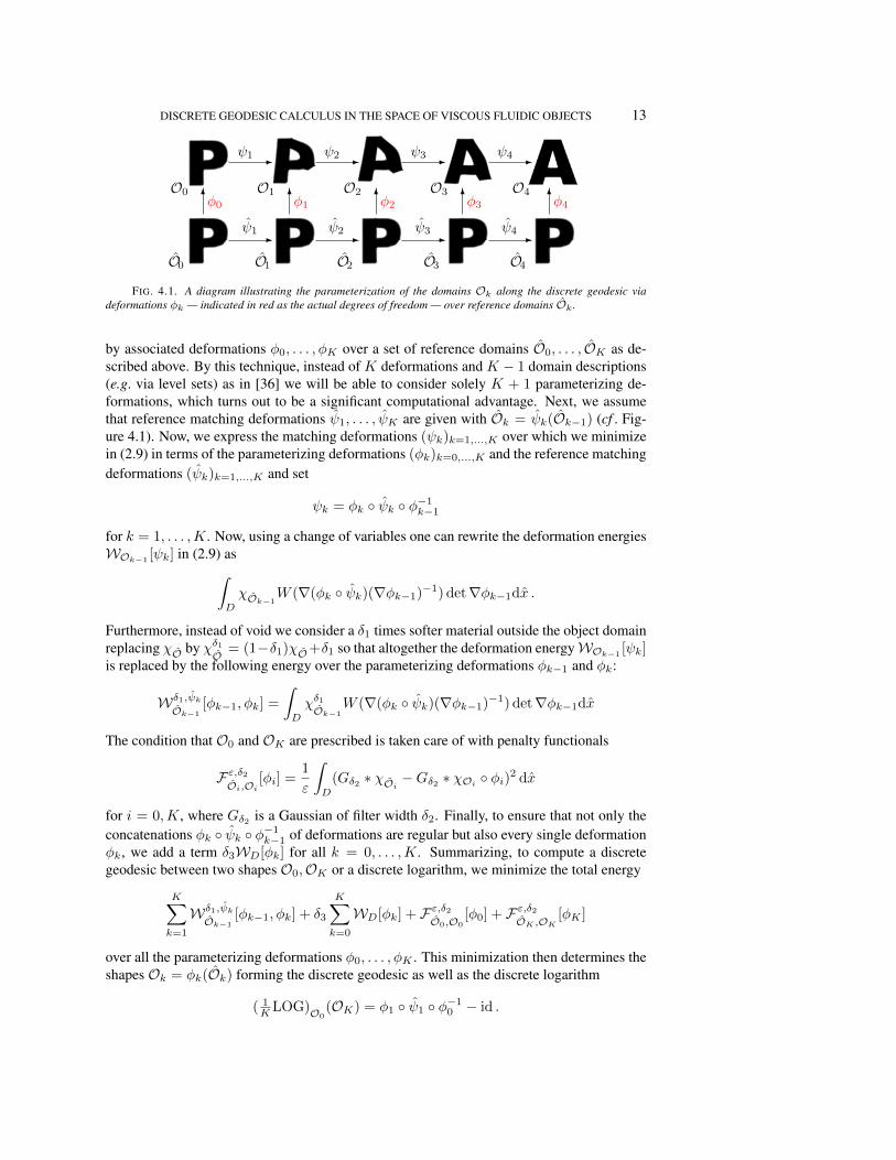
FIG. 4.1. A diagram illustrating the parameterization of the domains Ok along the discrete geodesic viadeformations φk — indicated in red as the actual degrees of freedom — over reference domains Ok .

by associated deformations φ0, . . . , φK over a set of reference domains O0, . . . , OK as de-scribed above. By this technique, instead of K deformations and K − 1 domain descriptions(e.g. via level sets) as in [36] we will be able to consider solely K + 1 parameterizing de-formations, which turns out to be a significant computational advantage. Next, we assumethat reference matching deformations ψ1, . . . , ψK are given with Ok = ψk(Ok−1) (cf . Fig-ure 4.1). Now, we express the matching deformations (ψk)k=1,...,K over which we minimizein (2.9) in terms of the parameterizing deformations (φk)k=0,...,K and the reference matchingdeformations (ψk)k=1,...,K and set

ψk = φk ◦ ψk ◦ φ−1k−1

for k = 1, . . . ,K. Now, using a change of variables one can rewrite the deformation energiesWOk−1

[ψk] in (2.9) as∫D

χOk−1W (∇(φk ◦ ψk)(∇φk−1)−1) det∇φk−1dx .

Furthermore, instead of void we consider a δ1 times softer material outside the object domainreplacing χO by χδ1

O= (1−δ1)χO+δ1 so that altogether the deformation energyWOk−1

[ψk]is replaced by the following energy over the parameterizing deformations φk−1 and φk:

Wδ1,ψkOk−1

[φk−1, φk] =

∫D

χδ1Ok−1

W (∇(φk ◦ ψk)(∇φk−1)−1) det∇φk−1dx

The condition that O0 and OK are prescribed is taken care of with penalty functionals

Fε,δ2Oi,Oi

[φi] =1

ε

∫D

(Gδ2 ∗ χOi −Gδ2 ∗ χOi ◦ φi)2 dx

for i = 0,K, where Gδ2 is a Gaussian of filter width δ2. Finally, to ensure that not only theconcatenations φk ◦ ψk ◦ φ−1k−1 of deformations are regular but also every single deformationφk, we add a term δ3WD[φk] for all k = 0, . . . ,K. Summarizing, to compute a discretegeodesic between two shapes O0,OK or a discrete logarithm, we minimize the total energy

K∑k=1

Wδ1,ψkOk−1

[φk−1, φk] + δ3

K∑k=0

WD[φk] + Fε,δ2O0,O0

[φ0] + Fε,δ2OK ,OK

[φK ]

over all the parameterizing deformations φ0, . . . , φK . This minimization then determines theshapes Ok = φk(Ok) forming the discrete geodesic as well as the discrete logarithm

( 1KLOG)O0

(OK) = φ1 ◦ ψ1 ◦ φ−10 − id .


K=8

K=4

K=2

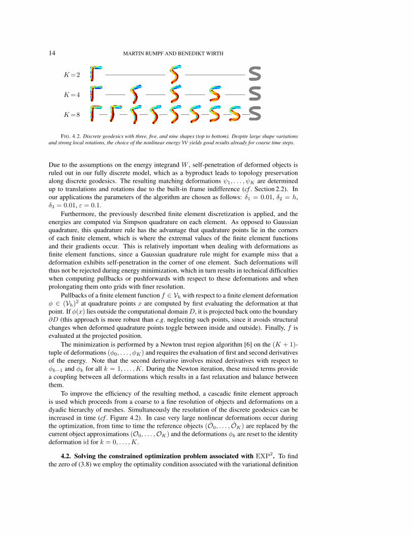
FIG. 4.2. Discrete geodesics with three, five, and nine shapes (top to bottom). Despite large shape variationsand strong local rotations, the choice of the nonlinear energyW yields good results already for coarse time steps.

Due to the assumptions on the energy integrand W , self-penetration of deformed objects isruled out in our fully discrete model, which as a byproduct leads to topology preservationalong discrete geodesics. The resulting matching deformations ψ1, . . . , ψK are determinedup to translations and rotations due to the built-in frame indifference (cf . Section 2.2). Inour applications the parameters of the algorithm are chosen as follows: δ1 = 0.01, δ2 = h,δ3 = 0.01, ε = 0.1.

Furthermore, the previously described finite element discretization is applied, and theenergies are computed via Simpson quadrature on each element. As opposed to Gaussianquadrature, this quadrature rule has the advantage that quadrature points lie in the cornersof each finite element, which is where the extremal values of the finite element functionsand their gradients occur. This is relatively important when dealing with deformations asfinite element functions, since a Gaussian quadrature rule might for example miss that adeformation exhibits self-penetration in the corner of one element. Such deformations willthus not be rejected during energy minimization, which in turn results in technical difficultieswhen computing pullbacks or pushforwards with respect to these deformations and whenprolongating them onto grids with finer resolution.

Pullbacks of a finite element function f ∈ Vh with respect to a finite element deformationφ ∈ (Vh)2 at quadrature points x are computed by first evaluating the deformation at thatpoint. If φ(x) lies outside the computational domainD, it is projected back onto the boundary∂D (this approach is more robust than e.g. neglecting such points, since it avoids structuralchanges when deformed quadrature points toggle between inside and outside). Finally, f isevaluated at the projected position.

The minimization is performed by a Newton trust region algorithm [6] on the (K + 1)-tuple of deformations (φ0, . . . , φK) and requires the evaluation of first and second derivativesof the energy. Note that the second derivative involves mixed derivatives with respect toφk−1 and φk for all k = 1, . . . ,K. During the Newton iteration, these mixed terms providea coupling between all deformations which results in a fast relaxation and balance betweenthem.

To improve the efficiency of the resulting method, a cascadic finite element approachis used which proceeds from a coarse to a fine resolution of objects and deformations on adyadic hierarchy of meshes. Simultaneously the resolution of the discrete geodesics can beincreased in time (cf . Figure 4.2). In case very large nonlinear deformations occur duringthe optimization, from time to time the reference objects (O0, . . . , OK) are replaced by thecurrent object approximations (O0, . . . ,OK) and the deformations φk are reset to the identitydeformation id for k = 0, . . . ,K.

4.2. Solving the constrained optimization problem associated with EXP2. To findthe zero of (3.8) we employ the optimality condition associated with the variational definition


of ( 12LOG). Indeed, for given ζ we introduce two deformations ψ1, ψ2 and corresponding

objects O2 := (ψ2 ◦ (id + ζ)) (O), O1 := ψ1(O). Now, we associate to the discrete path(O, O1, O2) with underlying deformations ψ1, ψ2 the energy

E [ψ1, ψ2] :=

∫OW (∇ψ1) dx+

∫ψ1(O)

W(∇(ψ2 ◦ (id + ζ) ◦ ψ−11 )

)dx .

We obtain ∂ψ1E [ψ1, ψ2] = 0 as the necessary condition to ensure that E [ψ1, ψ2] actually rep-

resents the path energy in (2.9) connecting the two objects O and O2 via a discrete geodesicof order 2 with the intermediate object ψ1(O). In the notion of Section 3.2 the property of(O, O1, O2) to be a discrete geodesic can be phrased as ψ1(O) = O1[O2]. Thus, a necessarycondition for (3.7) to hold is given by the condition

∂ψ1E [ψ1, ψ2] |ψ1=id+ζ = 0 (4.1)

for the remaining unknown ψ2. With respect to the algorithmic realization we reformulateand regularized the energy as described in Section 4.1 above to yield

Eδ1 [ψ1, ψ2] =

∫D

χδ1O(W (∇ψ1) +W (∇(ψ2 ◦ (id + ζ))(∇ψ1)−1) det∇ψ1

)dx .

Now, the discrete counterpart of (4.1) is the condition

0 = ∂ψ1Eδ1 [ψ1, ψ2]

∣∣ψ1=id+ζ

(θ)

=

∫D

χδ1O

(DW (∇(id + ζ)) : ∇θ

− DW (∇ψ2 ◦ (id + ζ)) : (∇ψ2 ◦ (id + ζ))∇θ (1+∇ζ)−1 det(1+∇ζ)

+ W (∇ψ2 ◦ (id + ζ)) det(1+∇ζ) tr((1+∇ζ)−1∇θ))

dx , (4.2)

where A : B = tr(ATB) for matrices A,B ∈ R2,2. This equation has to hold for all testdeformations θ. In our finite element context, the corresponding test functions are taken to beall finite element basis functions so that (4.2) becomes a system of nonlinear equations whichis solved for ψ2 via Newton’s method. Here too, we first find ψ2 on a coarse grid and thenuse the result as initialization of Newton’s method on finer grids.

5. Conclusions and outlook. Based on a variational time discretization of geodesicpaths in shape space we have proposed a novel time discrete geodesic calculus, which consistsof discrete logarithmic and exponential maps, discrete parallel transport and a discrete con-nection. We demonstrate how to use this discrete calculus as a robust and efficient toolbox forshape morphing, shape extrapolation, and transport of shape features along paths of shapes.Although in this expository article we restricted ourselves to two-dimensional objects, theapproach can be carried over to 3D viscous-fluid shapes. The concept can also be adapted todeformations of hypersurfaces and corresponding deformation energies, which measure tan-gential as well as normal bending stresses [11, 21]. For example, a generalization to the spaceof planar elastic curves and thin shell surfaces is feaible. Furthermore, instead of a metricstructure induced by the viscous flow paradigm, the Wasserstein distance of optimal transportcan be considered [35]. It this case the time discretization of the Monge–Kantorovich prob-lem proposed by Benamou and Brenier [4] is a possible starting point. Beyond these futuredirections of generalization, a theoretical foundation has to be established with existence andregularity results for the above-mentioned infinite dimensional shape spaces. Furthermore,


the limit behaviour of the discrete geodesic calculus for vanishing time step size and the con-vergence of the discrete path energy to the corresponding continuous path energy in the senseof Γ-convergence has to be investigated (cf . the work by Muller and Ortiz on Γ-convergenceof a time discrete action functional in the case of Hamiltonian systems [28]). Finally, giventhe notion of a time discrete transport, the relation of the curvature tensor to the parallel trans-port along the edges of a quadrilateral (cf . Proposition 1.5.8. in [18]) can be used to definea time discrete curvature tensor, which then allows an exploration of the local geometry ofshape space.

Acknowledgment Benedikt Wirth was supported by the German Science Founda-tion via the Hausdorff Center of Mathematics and by the Federal Ministry of Education andResearch via CROP.SENSe.net.

REFERENCES

[1] MARTIN BAUER AND MARTINS BRUVERIS, A new Riemannian setting for surface registration, in Proceed-ings of the Mathematical Foundations in Computational Anatomy workshop, Xavier Pennec, SarangJoshi, and Mads Nielsen, eds., 2011, pp. 182–193.

[2] M. F. BEG, M.I. MILLER, A. TROUVE, AND L. YOUNES, Computational anatomy: Computing metrics onanatomical shapes, in Proceedings of 2002 IEEE ISBI, 2002, pp. 341–344.

[3] M. FAISAL BEG, MICHAEL I. MILLER, ALAIN TROUVE, AND LAURENT YOUNES, Computing large de-formation metric mappings via geodesic flows of diffeomorphisms, International Journal of ComputerVision, 61 (2005), pp. 139–157.

[4] JEAN-DAVID BENAMOU AND YANN BRENIER, A computational fluid mechanics solution to the Monge-Kantorovich mass transfer problem, Numer. Math., 84 (2000), pp. 375–393.

[5] PHILIPPE G. CIARLET, Mathematical Elasticity, Vol. I: Three–Dimensional Elasticity, Studies in Mathematicsand its Applications, Elsevier, Amsterdam, 1997.

[6] A. R. CONN, N. I. M GOULD, AND P. L. TOINT, Trust-Region Methods, SIAM, 2000.[7] D. DUPUIS, U. GRENANDER, AND M.I. MILLER, Variational problems on flows of diffeomorphisms for

image matching, Quarterly of Applied Mathematics, 56 (1998), pp. 587–600.[8] J. EHLERS, F. A. E. PIRANI, AND A. SCHILD, The geometry of free fall and light propagation, in General

relativity (papers in honour of J. L. Synge), Clarendon Press, Oxford, 1972, pp. 63–84.[9] P.T. FLETCHER, CONGLIN LU, S.M. PIZER, AND SARANG JOSHI, Principal geodesic analysis for the study

of nonlinear statistics of shape, Medical Imaging, IEEE Transactions on, 23 (2004), pp. 995–1005.[10] P. FLETCHER AND R. WHITAKER, Riemannian metrics on the space of solid shapes, in MICCAI 2006: Med

Image Comput Comput Assist Interv., 2006.[11] GERO FRIESECKE, RICHARD JAMES, MARIA GIOVANNA MORA, AND STEFAN MULLER, Derivation of

nonlinear bending theory for shells from three-dimensional nonlinear elasticity by Gamma-convergence,C. R. Math. Acad. Sci. Paris 336, 8 (2003), pp. 697–702.

[12] MATTHIAS FUCHS, BERT JUTTLER, OTMAR SCHERZER, AND HUAIPING YANG, Shape metrics based onelastic deformations, J. Math. Imaging Vis., 35 (2009), pp. 86–102.

[13] M. FUCHS AND O. SCHERZER, Regularized reconstruction of shapes with statistical a priori knowledge,International Journal of Computer Vision, 79 (2008), pp. 119–135.

[14] ST. HAKER, A. TANNENBAUM, AND R. KIKINIS, Mass preserving mappings and image registration, Pro-ceedings of Fourth International Conference on Medical Image Computing and Computer-Assisted Inter-vention, (2001), pp. 120–127.

[15] ARKADY KHEYFETS, WARNER A. MILLER, AND GREGORY A. NEWTON, Schild’s ladder parallel transportprocedure for an arbitrary connection, Internat. J. Theoret. Phys., 39 (2000), pp. 2891–2898.

[16] M. KILIAN, N. J. MITRA, AND H. POTTMANN, Geometric modeling in shape space, in ACM Transactionson Graphics, vol. 26, 2007, pp. #64, 1–8.

[17] E. KLASSEN, A. SRIVASTAVA, W. MIO, AND S. H. JOSHI, Analysis of planar shapes using geodesic paths onshape spaces, IEEE Transactions on Pattern Analysis and Machine Intelligence, 26 (2004), pp. 372–383.

[18] WILHELM P. A. KLINGENBERG, Riemannian geometry, vol. 1 of de Gruyter Studies in Mathematics, Walterde Gruyter & Co., Berlin, second ed., 1995.


[19] S. KURTEK, E. KLASSEN, Z. DING, AND A. SRIVASTAVA, A novel Riemannian framework for shape anal-ysis of 3d objects, in IEEE Computer Vision and Pattern Recognition (CVPR), 2010.

[20] S. KURTEK, E. KLASSEN, J. GORE, Z. DING, AND A. SRIVASTAVA, Elastic geodesic paths in shape spaceof parametrized surfaces, Pattern Analysis and Machine Intelligence, IEEE Transactions on, to appear(2011).

[21] N. LITKE, M. DROSKE, M. RUMPF, AND P. SCHRODER, An image processing approach to surface matching,in Third Eurographics Symposium on Geometry Processing, M. Desbrun and H. Pottmann, eds., 2005,pp. 207–216.

[22] XIUWEN LIU, YONGGANG SHI, IVO DINOV, AND WASHINGTON MIO, A computational model of multidi-mensional shape, International Journal of Computer Vision, Online First (2010).

[23] MARCO LORENZI, NICHOLAS AYACHE, AND XAVIER PENNEC, Schilds ladder for the parallel transportof deformations in time series of images, in Proceedings of Information Processing in Medical Imaging(IPMI’11), G. Szekely and H. Hahn, eds., vol. 6801 of LNCS, 2011, pp. 463–474.

[24] A. MENNUCCI, S. SOATTO, G. SUNDARAMOORTHI, AND A. YEZZI, A new geometric metric in the spaceof curves, and applications to tracking deforming objects by prediction and filtering, Siam Journal onImaging Sciences, (2011), p. to appear.

[25] PETER W. MICHOR AND DAVID MUMFORD, Riemannian geometries on spaces of plane curves, J. Eur. Math.Soc., 8 (2006), pp. 1–48.

[26] M. I. MILLER, A. TROUVE, AND L. YOUNES, The metric spaces, Euler equations, and normal geodesicimage motions of computational anatomy, in Proceedings of the 2003 International Conference on ImageProcessing, vol. 2, IEEE, 2003, pp. 635–638.

[27] M. I. MILLER AND L. YOUNES, Group actions, homeomorphisms, and matching: a general framework,International Journal of Computer Vision, 41 (2001), pp. 61–84.

[28] S. MULLER AND M. ORTIZ, On the Γ-convergence of discrete dynamics and variational integrators, J. Non-linear Sci., 14 (2004), pp. 279–296.

[29] XAVIER PENNEC AND MARCO LORENZI, Which parallel transport for the statistical analysis of longitudinaldeformations?, in Colloque GRETSI ’11, September 2011.

[30] F. R. SCHMIDT, M. CLAUSEN, AND D. CREMERS, Shape matching by variational computation of geodesicson a manifold, in Pattern Recognition, vol. 4174 of LNCS, Springer, 2006, pp. 142–151.

[31] ANUJ SRIVASTAVA, AASTHA JAIN, SHANTANU JOSHI, AND DAVID KAZISKA, Statistical shape mod-els using elastic-string representations, in Asian Conference on Computer Vision, P.J. Narayanan, ed.,vol. 3851 of LNCS, 2006, pp. 612–621.

[32] ANUJ SRIVASTAVA, ERIC KLASSEN, SHANTANU H. JOSHI, AND IAN H. JERMYN, Shape analysis of elasticcurves in euclidean spaces, Pattern Analysis and Machine Intelligence, IEEE Transactions on, 33 (2011),pp. 1415–1428.

[33] GANESH SUNDARAMOORTHI, ANDREA MENNUCCI, STEFANO SOATTO, AND ANTHONY YEZZI, A newgeometric metric in the space of curves, and applications to tracking deforming objects by prediction andfiltering, SIAM Journal on Imaging Sciences, 4 (2011), pp. 109–145.

[34] G. SUNDARAMOORTHI, A. YEZZI, AND A. MENNUCCI, Sobolev active contours, International Journal ofComputer Vision., 73 (2007), pp. 345–366.

[35] CRIC VILLANI, Topics in Optimal Transportation, Mathematical Surveys and Monographs, American Math-ematical Society, Providence, RI, 2003.

[36] BENEDIKT WIRTH, LEAH BAR, MARTIN RUMPF, AND GUILLERMO SAPIRO, A continuum mechanicalapproach to geodesics in shape space, IJCV, 93 (2011), pp. 293–318.

[37] LAURENT YOUNES, PETER W. MICHOR, JAYANT SHAH, AND DAVID MUMFORD, A metric on shape spacewith explicit geodesics, Atti Accad. Naz. Lincei Cl. Sci. Fis. Mat. Natur. Rend. Lincei (9) Mat. Appl., 19(2008), pp. 25–57.

[38] LEI ZHU, YAN YANG, STEVEN HAKER, AND ALLEN TANNENBAUM, An image morphing technique basedon optimal mass preserving mapping, IEEE Transactions on Image Processing, 16 (2007), pp. 1481–1495.

[39] JEAN-PAUL ZOLESIO, Shape topology by tube geodesic, in IFIP Conference on System Modeling and Opti-mization No 21,, 2004, pp. 185–204.

Documents

DISCRETE GEODESIC CALCULUS IN THE SPACE …numod.ins.uni-bonn.de/research/papers/public/RuWi12.pdfGeodesic paths in shape space allow to ... path establishes correspondences between