H. C. So Page 1 Semester B, 2011-2012

Discrete-Time Fourier Transform (DTFT) Chapter Intended Learning Outcomes: (i) Understanding the characteristics and properties of DTFT (ii) Ability to perform discrete-time signal conversion between the time and frequency domains using DTFT and inverse DTFT

H. C. So Page 2 Semester B, 2011-2012

Definition

DTFT is a frequency analysis tool for aperiodic discrete-time signals The DTFT of , , has been derived in (5.4):

(6.1)

The derivation is based on taking the Fourier transform of of (5.2)

As in Fourier transform, is also called spectrum and is

a continuous function of the frequency parameter Is DTFT complex? Is it periodic?

H. C. So Page 3 Semester B, 2011-2012

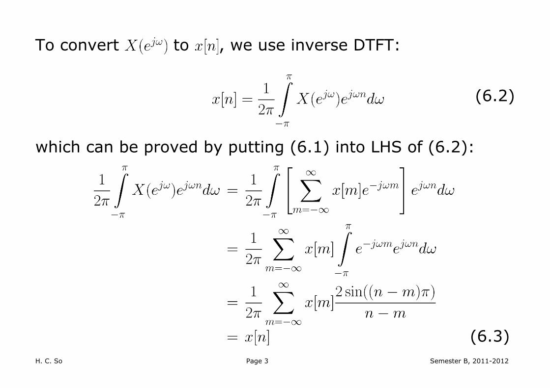
To convert to , we use inverse DTFT:

(6.2)

which can be proved by putting (6.1) into LHS of (6.2):

(6.3)

H. C. So Page 4 Semester B, 2011-2012

discrete and aperiodic continuous and periodic

time domain frequency domain

... ...

Fig.6.1: Illustration of DTFT

H. C. So Page 5 Semester B, 2011-2012

is continuous and periodic with a period of

is generally complex, we can illustrate using the

magnitude and phase spectra, i.e., and :

(6.4)

and

(6.5)

where both are continuous in frequency and periodic. Convergence of DTFT

The DTFT of a sequence converges if

H. C. So Page 6 Semester B, 2011-2012

(6.6)

Recall (5.10) and assume the transform of converges

for region of convergence (ROC) of :

(6.7)

When ROC includes the unit circle:

(6.8)

which leads to the convergence condition for . This

also proves the P2 property of the transform.

H. C. So Page 7 Semester B, 2011-2012

Let be the impulse response of a linear time-invariant

(LTI) system, the following three statements are equivalent: S1. ROC for the transform of includes unit circle

S2. The system is stable so that

S3. The DTFT of , i.e., , converges

Note that is also known as system frequency response

Example 6.1 Determine the DTFT of .

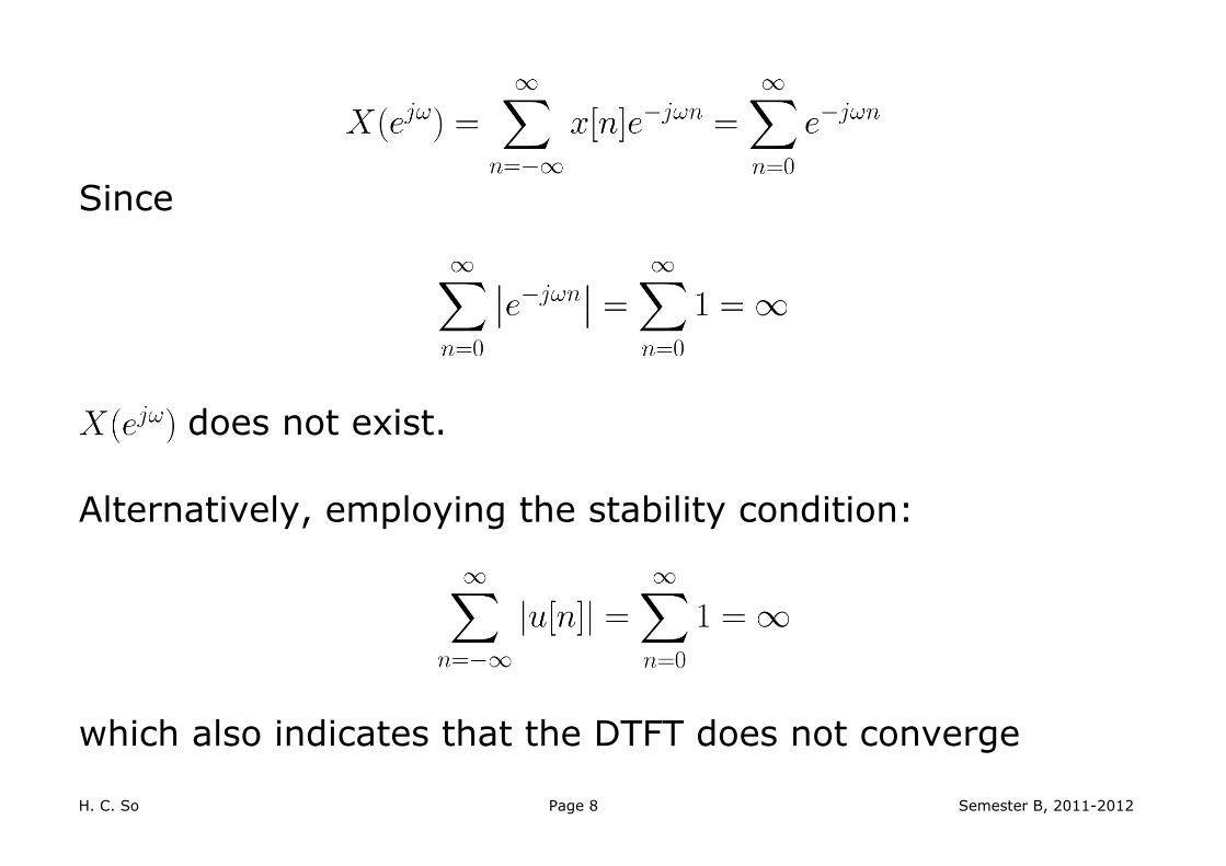
Using (6.1), the DTFT of is computed as:

H. C. So Page 8 Semester B, 2011-2012

Since

does not exist.

Alternatively, employing the stability condition:

which also indicates that the DTFT does not converge

H. C. So Page 9 Semester B, 2011-2012

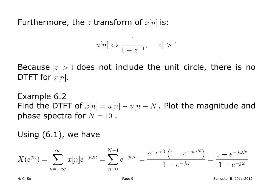
Furthermore, the transform of is:

Because does not include the unit circle, there is no

DTFT for .

Example 6.2 Find the DTFT of . Plot the magnitude and

phase spectra for . Using (6.1), we have

H. C. So Page 10 Semester B, 2011-2012

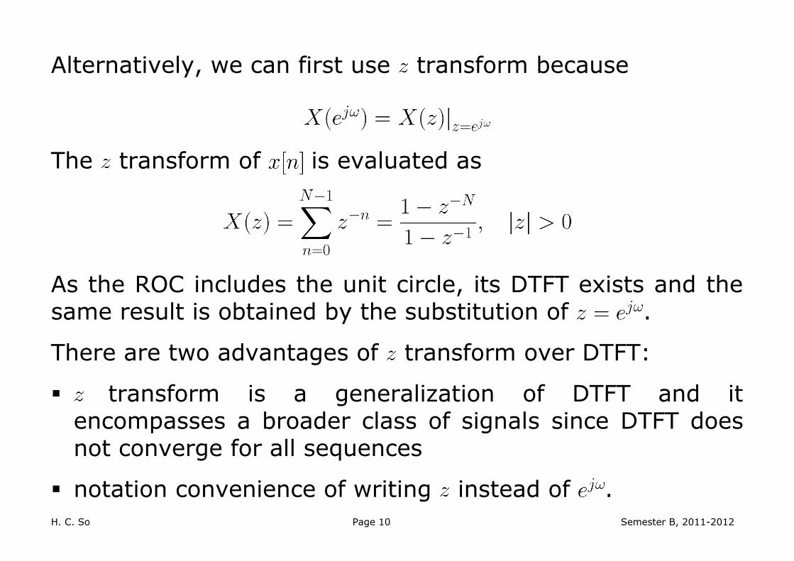
Alternatively, we can first use transform because

The transform of is evaluated as

As the ROC includes the unit circle, its DTFT exists and the same result is obtained by the substitution of .

There are two advantages of transform over DTFT:

transform is a generalization of DTFT and it encompasses a broader class of signals since DTFT does not converge for all sequences

notation convenience of writing instead of .

H. C. So Page 11 Semester B, 2011-2012

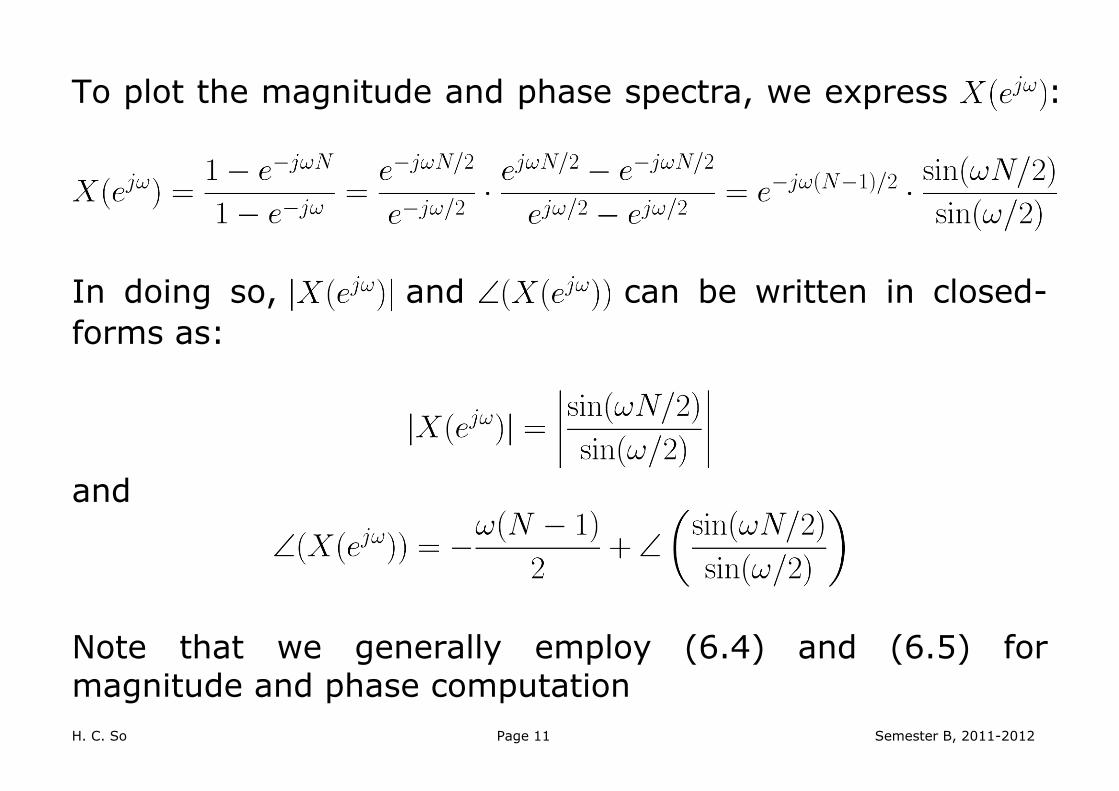
To plot the magnitude and phase spectra, we express :

In doing so, and can be written in closed-

forms as:

and

Note that we generally employ (6.4) and (6.5) for magnitude and phase computation

H. C. So Page 12 Semester B, 2011-2012

In using MATLAB to plot and , we utilize the

command sinc so that there is no need to separately

handle the “0/0” cases due to the sine functions Recall the definition of sinc function:

As a result, we have:

H. C. So Page 13 Semester B, 2011-2012

The key MATLAB code for is N=10; %N=10

w=0:0.01*pi:2*pi; %successive frequency point

%separation is 0.01pi

dtft=N.*sinc(w.*N./2./pi)./(sinc(w./2./pi)).*exp(-

j.*w.*(N-1)./2); %define DTFT function

subplot(2,1,1)

Mag=abs(dtft); %compute magnitude

plot(w./pi,Mag); %plot magnitude

subplot(2,1,2)

Pha=angle(dtft); %compute phase

plot(w./pi,Pha); %plot phase

Analogous to Example 4.4, there are 201 uniformly-spaced points to approximate the continuous functions and

.

H. C. So Page 14 Semester B, 2011-2012

0 0.5 1 1.5 20

5

10Magnitude Response

/

0 0.5 1 1.5 2-4

-2

0

2

4Phase Response

/

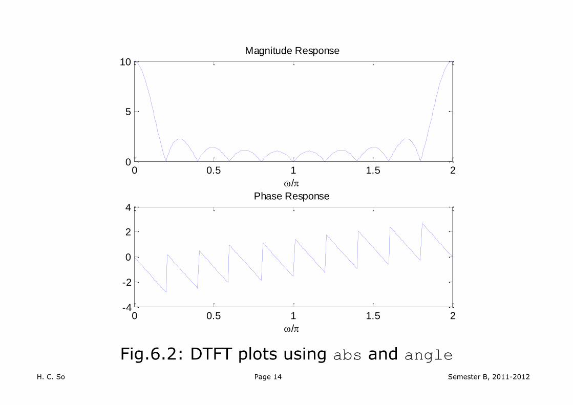
Fig.6.2: DTFT plots using abs and angle

H. C. So Page 15 Semester B, 2011-2012

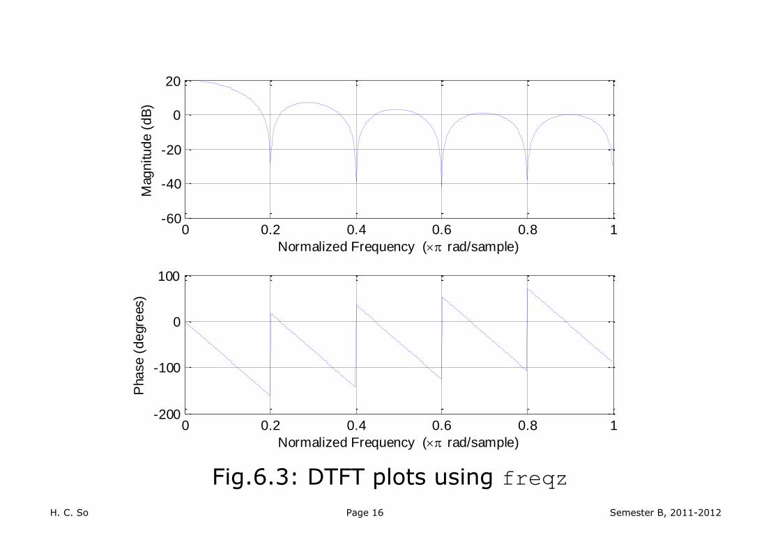
Alternatively, we can use the command freqz:

which is ratio of two polynomials in The corresponding MATLAB code is: N=10; %N=10

a=[1,-1]; %vector for denominator

b=[1,zeros(1,N-1),-1]; %vector for numerator

freqz(b,a) %plot magnitude & phase (dB)

Note that it is also possible to use and in

this case we have b=ones(N,1) and a=1.

H. C. So Page 16 Semester B, 2011-2012

0 0.2 0.4 0.6 0.8 1-200

-100

0

100

Normalized Frequency ( rad/sample)

Pha

se (

de

gre

es)

0 0.2 0.4 0.6 0.8 1-60

-40

-20

0

20

Normalized Frequency ( rad/sample)

Mag

nitu

de (

dB

)

Fig.6.3: DTFT plots using freqz

H. C. So Page 17 Semester B, 2011-2012

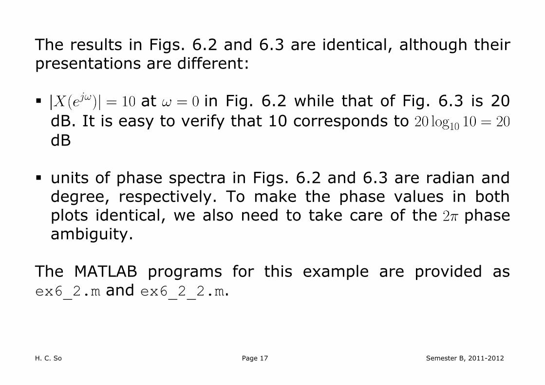
The results in Figs. 6.2 and 6.3 are identical, although their presentations are different: at in Fig. 6.2 while that of Fig. 6.3 is 20

dB. It is easy to verify that 10 corresponds to

dB units of phase spectra in Figs. 6.2 and 6.3 are radian and

degree, respectively. To make the phase values in both plots identical, we also need to take care of the phase ambiguity.

The MATLAB programs for this example are provided as ex6_2.m and ex6_2_2.m.

H. C. So Page 18 Semester B, 2011-2012

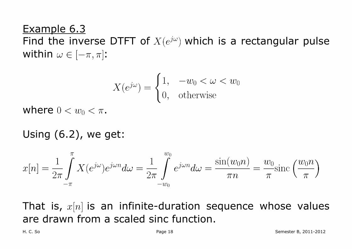
Example 6.3 Find the inverse DTFT of which is a rectangular pulse

within :

where . Using (6.2), we get:

That is, is an infinite-duration sequence whose values

are drawn from a scaled sinc function.

H. C. So Page 19 Semester B, 2011-2012

Example 6.4 Determine the inverse DTFT of which has the form of:

With the use of , the corresponding transform is

Note that ROC should include the unit circle as DTFT exists Employing the time shifting property, we get

H. C. So Page 20 Semester B, 2011-2012

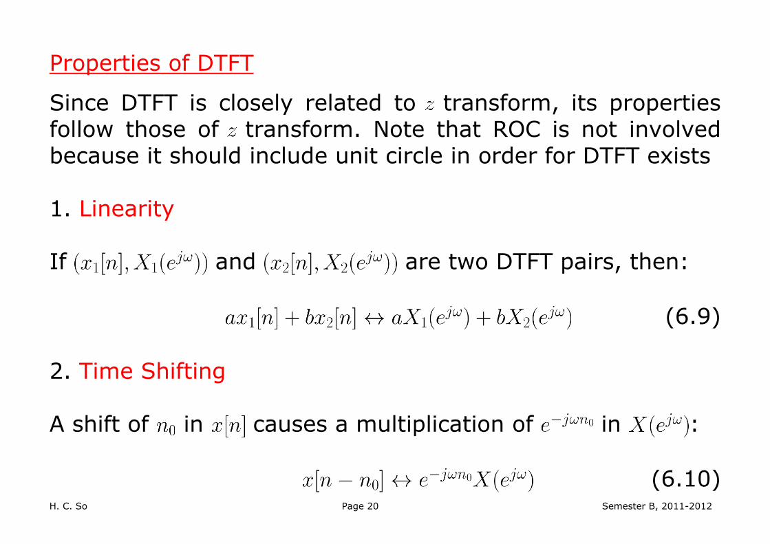
Properties of DTFT

Since DTFT is closely related to transform, its properties follow those of transform. Note that ROC is not involved because it should include unit circle in order for DTFT exists 1. Linearity If and are two DTFT pairs, then:

(6.9)

2. Time Shifting A shift of in causes a multiplication of in :

(6.10)

H. C. So Page 21 Semester B, 2011-2012

3. Multiplication by an Exponential Sequence Multiplying by in time domain corresponds to a shift

of in the frequency domain:

(6.11)

which agrees with (5.33) by putting and 4. Differentiation Differentiating with respect to corresponds to

multiplying by :

(6.12)

H. C. So Page 22 Semester B, 2011-2012

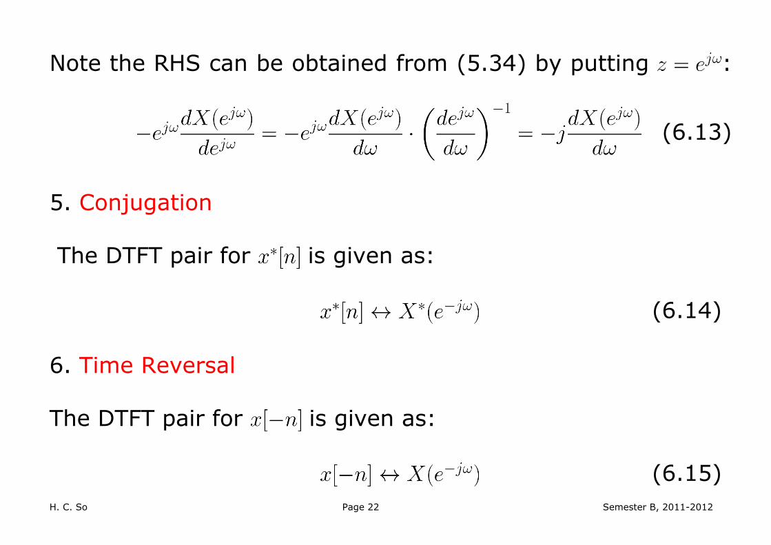
Note the RHS can be obtained from (5.34) by putting :

(6.13)

5. Conjugation The DTFT pair for is given as:

(6.14)

6. Time Reversal The DTFT pair for is given as:

(6.15)

H. C. So Page 23 Semester B, 2011-2012

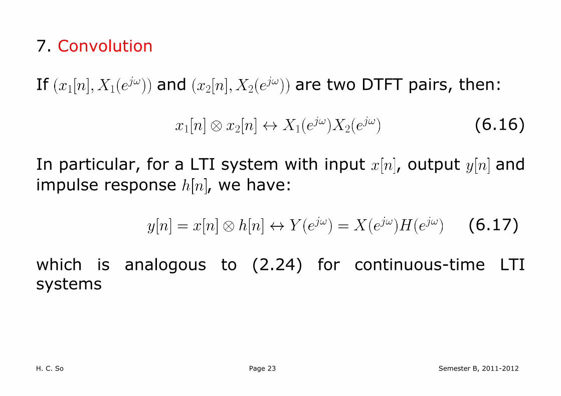
7. Convolution If and are two DTFT pairs, then:

(6.16)

In particular, for a LTI system with input , output and

impulse response , we have:

(6.17)

which is analogous to (2.24) for continuous-time LTI systems

H. C. So Page 24 Semester B, 2011-2012

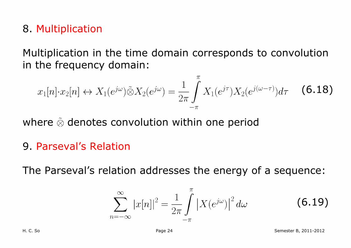
8. Multiplication Multiplication in the time domain corresponds to convolution in the frequency domain:

(6.18)

where denotes convolution within one period 9. Parseval’s Relation The Parseval’s relation addresses the energy of a sequence:

(6.19)

H. C. So Page 25 Semester B, 2011-2012

With the use of (6.2), the proof is:

(6.20)