Discrete-time Sliding Mode Control of the RRR-robot

Discrete-time Sliding Mode Control of the RRR-robot

G.M. van der Zalm

DCT - 2003.82

Supervision

M.Sc. Dragan Kostic dr. ir. Bram die Jager

Eindhoven University of Technology Department of Mechanical Engineering Control Systems Technology

Contents

1 Introduction 5

Discussion of the control algorithm 7 . . . . . . . . . . . . . . . . . . . . . . . . . . . . . . . 2.1 System definition in discrete time 7

. . . . . . . . . . . . . . . . . . . . . . . . . . . . . . . . . . . . . . . . 2.2 Control strategy 7 2.2.1 Definition of the sliding manifold . . . . . . . . . . . . . . . . . . . . . . . . . . 7

. . . . . . . . . . . . . . . . . . . . . . . . . . . . . . . . . . . . . . 2.2.2 Control law 8 . . . . . . . . . . . . . . . . . . . . . . . . . . . . . . 2.2.3 Design of sliding manifold 8

. . . . . . . . . . . . . . . . . . . . . . . . . . . . . . . . . . . . . . . . . 2.3 Reaching law 9 . . . . . . . . . . . . . . . . . . . . . . . . . . . . . . . . . . . . . . . . . . . 2.4 Simulation 9

. . . . . . . . . . . . . . . . . . . . . . . . . . . . . . . . . . . . 2.4.1 No disturbance 9 . . . . . . . . . . . . . . . . . . . . . . . . . . . . . . . . . . . . . . 2.4.2 Disturbance 10

3 Implementation on the RRR-robot 11 . . . . . . . . . . . . . . . . . . . . . . . . . . . . . . . . . . . . . . 3.1 Reference trajectory 11

. . . . . . . . . . . . . . . . . . . . . . . . . . . . . . . . . . . . . . . . . 3.2 Identification 11 . . . . . . . . . . . . . . . . . . . . . . . . . . . . . . . . 3.3 Modification of the control law 12

. . . . . . . . . . . . . . . . . . . . . . . . . . . . . . . . . . . . . . . . 3.4 Observerdesign 13 . . . . . . . . . . . . . . . . . . . . . . . . . . . . . . . 3.5 Tuning the controller parameters 13

. . . . . . . . . . . . . . . . . . . . . . . . . . . . . . . . . . . . . . 3.5.1 Choice of a 13 . . . . . . . . . . . . . . . . . . . . . . . . . . . . . . . . . 3.5.2 Choiceofo, q a n d r 15

4 Results 17 . . . . . . . . . . . . . . . . . . . . . . . . . . . . 4.1 Results of the sliding mode controller 17

. . . . . . . . . . . . . . . . . . . . . . . . . . . . . . . . . . . . . . 4.1.1 Discussion 19 . . . . . . . . . . . . . . . . . . . . . . . . . . . . . . . 4.2 Comparison with H , controller 20

5 Conclusions & Recommendations 23

A Coordinate transformation 25

C Transfer function Kalman filter with controller 29

CONTENTS

Chapter 1

Introduction

The theory of Variable structure systems (VSS) with sliding mode control (SMC) has been developed for the last five decades 11-31, When designed in continuos-time domain, SMC systems can feature some distinguished characteristics: invariance to parameter uncertainties and external disturbances, system order reduction, predictable transient behaviour, etc. One of the underlying assumptions in the design and anal- ysis of VSS with SMC is that the control can be switched from one value to another infinitely fast. In practical systems, however, it is impossible to achieve infinite frequency of switching. This is especially impossible with discrete time implementation of SMC algorithms, when finite time delays for control com- putation are present. Without switching control at infinite rate, the distinguished features of SMC systems may not be feasible in practice. Additionally, chatterhg m q occur in the sliding and steady-state modes of SMC systems. In the steady-state, chattering appears as a high-frequency oscillation about the desired equilibrium point and may also serve as a source to excite unmodelled high-frequency dynamics of the system. To deal with problems caused by discrete-time implementation of SMC algorithms, several conceptual and methodological solutions have been proposed. The most important conceptual contribution is the development of discrete-time SMC algorithms [4,5] that directly take into account effects of discretiza- tion. Methodological solutions are directed at eliminating or reducing effects of chattering 11-31. A discrete time SMC algorithm, considered in 16-81, utilizes both conceptual and methodological advances of SMC theory. It ensures that the sliding mode is reached in finite time without negative chattering effects. Addi- tionally, above mentioned distinguished characteristics of VSS with SMC are preserved - the algorithm is proven to be robust against parameter uncertainties, as well as external disturbances, it enables nice control over transient behaviour of the controlled system, and the system order is reduced in sliding mode. The exceptional property of the considered SMC algorithm is simplicity of its feedback control law, which can be implemented on-line with a minimum computational effort. In this project, effects of the discrete-time SMC algorithm 16-81 in the robot motion control problem should be investigated. The RRR robot 19-101, installed in the Dynamics and Control Laboratory at the Department of Mechanical Engineering, is the experimental set-up used for this investigation. Because of the interactions between the three joints, the RRR robot is quite difficult for accurate and robust control. To facilitate model-based control, a nonlinear robot dynamic model is derived in closed-form and its parameters are experimentally estimated with sufficient accuracy [11,12]. The model is implemented in MatlabISimulink for real-time application [13]. Enhanced performance of motion control using the nonlinear dynamic model in combination with a linear H , feedback law has been recognized and reported in [14] already. Drawback of the H, feedback is the relative high-order of the controller, which may look less appealing for use in practice. Purpose of this project is to investigate whether the discrete-time SMC law can provide similar performance as the H , feedback but with less on-line computational effort. This report presents the results obtained after six weeks work on the project. It is organized as follows. First, the discrete-time SMC algorithm is worked out theoretically, and verified in simulations. Then, identification of the RRR robot dynamics, that are not compensated with the dynamic model, is done. The discrete-time SMC law is designed upon the identified dynamics. The controller is tested in experiments on the RRR-robot, and compared with the results of the H, controller. Finally, conclusions are drawn and recommendation for further research are given.

1 Introduction

Chapter 2

of the co trol algorithm

The control algorithm is discussed using the example in [8], in which a DC motor is considered as the controlled plant. First, the system will be defined in discrete time. Then, the calculation of the sliding manifold coefficients will be done and the control law will be defined. Finally, simulations are performed to validate the controller.

2.1 System definition in discrete time

Tfie considered plant is a DC motor, which can be described by the following continuous-time model:

where xl = Od - Q, with .9 the angular position of the shaft, Od the desired constant angle, xz = -w, with w the rotor velocity, z = [zl zzIT, and u the control signal. The discrete model of the system (2.1) can be calculated with [8]:

6z(kT) = As(T)x(kT) + bs(T)u(kT), (2.2)

where

As (T ) = v; bs (T) = $ J: eAT bd.r

In this discrete-time representation, 6x(kT) stands for forward difference, i.e. Gz(kT) = x((k'l)T)-x("T) T , and eAT is the fundamental matrix of the system. In the following, the notation (k) stands for (kT).

2.2 Control strategy

The control strategy is such that the state is driven to a so-called sliding manifold from any initial condition in finite time, and is forced to stay on it. The state x is driven to the sliding manifold in the reaching mode. If the state remains on the sliding manifold, the system is said to be in sliding mode. A desired sliding mode dynamics can be achieved by appropiate design of the sliding manifold. On this manifold, the system dynamics are of lower order, and the sliding mode is very robust with respect to modeling error and disturbances.

2.2.1 Definition of the sliding manifold

Let s = c g ( T ) s ; where cs(T) E IRlXn.

The sliding manifold is then defined as s = 0. With the assumption cb (T ) b6 (T ) = 1, the relative degree of s with respect to the control signal u is one.

2 Discussion of the control algorithm

2.2.2 Control law

The reaching law is defined as 6s = -@(s (k ) , X ( k ) )

where the function @(s; X ) will be defined later on, and

By substituting (2.2) into (2.6), and solving for u ( k ) , one obtains the control law

u ( k ) = -c , j (T)As(T)x(k) - Q j ( s ( k ) , X ( k ) ) . (2-7)

The function @ ( s , X) will be chosen such that the control law has two modes: a non-linear and a linear one. The linear mode acts in a vicinity of the sliding manifold. That vicinity, denoted by S ( T ) , is defined by:

2.2.3 Design of sliding manifold

The dynamics of the system on the sliding manifold are governed by the equation s = c ~ x = 0. This means that a desired behavior on the manifold can be obtained by calculating appropriate values for cd. In the following, the algorithm for this calculation will be discussed. First, the system (2.2) with the control law (2.7) is transformed into the following regular form:

by the coordinate transformation

Here, the matrices PI and Pz are given by equations (A.2-A.4), see appendix A. cs has to be designed in such a way, that the zero dynamics, i.e. the behavior of x ( k ) when s - 0, is such that x converges to zero. For s - 0, the system (2.9) is described by the relation

The eigenvalues of All are only determined by cl (T), and are free to choose. The desired eigenvalues 6i are chosen as

e-a ,T- l & ( T ) = - T > f f i > O : (2.12)

Then the elements of cl (T) are determined by

Finally, the vector c,j defining the sliding manifold is given by

c s ( T ) = [ s ( T ) j 1 ] p c l ( T ) .

2.3 Reaching law

2.3 Reaching law

Consider the perturbed system

where AAg (T ) E Rn xn is a matrix of uncertainties, dg ( T ) E IRn l , and f ( k ) a bounded external disturbance with 1 f ( k ) 1 < pVk E No. Assume that the matching conditions are given by:

It is proven in [8], that the following conditions on @ are sufficient for x to reach the sliding manifold in finite time and stay on it for each xo E Rn:

The first condition constitutes the linear mode of the control law, where the second and third condition are sufficient for s to reach S in finite time, and stay in it. Since the mapping @ is a continuous one in the vicinity S , the control law is also a continuous function, which results in a chattering free system. If the reaching function is chosen as

@ ( s , X ) = min(Y; a + q/sl + r l l X i / l ) s p ( s ) , 0 5 qT < 1, r 2 d,y, a > yp, (2.18)

the conditions (2.17) are satisfied. With this reaching function, the vicinity S is defined by:

If no disturbances are present, s equals zero one time step after it enters S , since the equation for 6s becomes:

The second and third condition of (2.17) guarantee that s stays in S , in face of the presence of disturbances.

2.4 Simulation

The control algorithm is validated by simulations in Simulink. First, a simulation without disturbance is done. Then, the robustness properties of the controller are investigated by performing simulations with a perturbed model.

2.4.1 No disturbance

The numerical values for the discrete-time system matrices with T = 0.4 ms are

The desired eigenvalue of All is chosen as Ji = -15. Then, the sliding manifold coefficients c~ as calculated by the MATLAB-routine calc-cd, see appendix B, are:

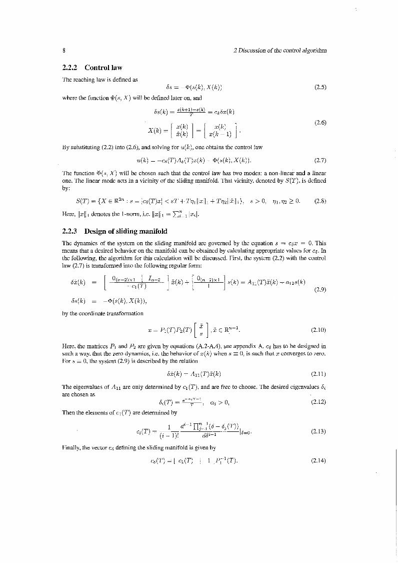
Simulation results with a = 8, q = 0 and r = 0 are shown in figure 2.1. It can be concluded that the sliding manifold is reached in finite time, and that the control input is chattering free.

10 2 Discussion of the control algorithm

Phase oortrait

0 0.2 0.4 0.6 0.8 1 Time [s]

1 5

0 5

0 ---- 2!L -0 5 0 0 2 0 4 06 0 8 1

Tme [s]

Figure 2.1: Simulation with u = 8, q = r = 0 and initial conditions zo = [I00 0IT

2.4.2 Disturbance

The perturbed system (2.15) is used, with the disturbance being a normally distributed white noise f . Taken into account the matching conditions (2.16), the model becomes:

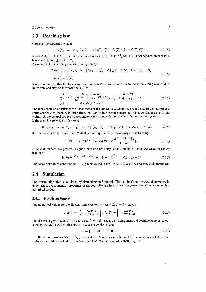
The noise amplitude p = 0.7 and the upperbound for the vector d is d , = 0.01. Then, according to equation 2.18, r > d,y and 7 > 1, r is set to 0.011. The influence of sampling time T on the simulation results for s and 8 is shown in figure 2.2. It is clear that a smaller sampling time improves the performance

Figure 2.2: Influence of sampling time T on s and 8

of the controller.

Chapter 3

3.1 Reference trajectory

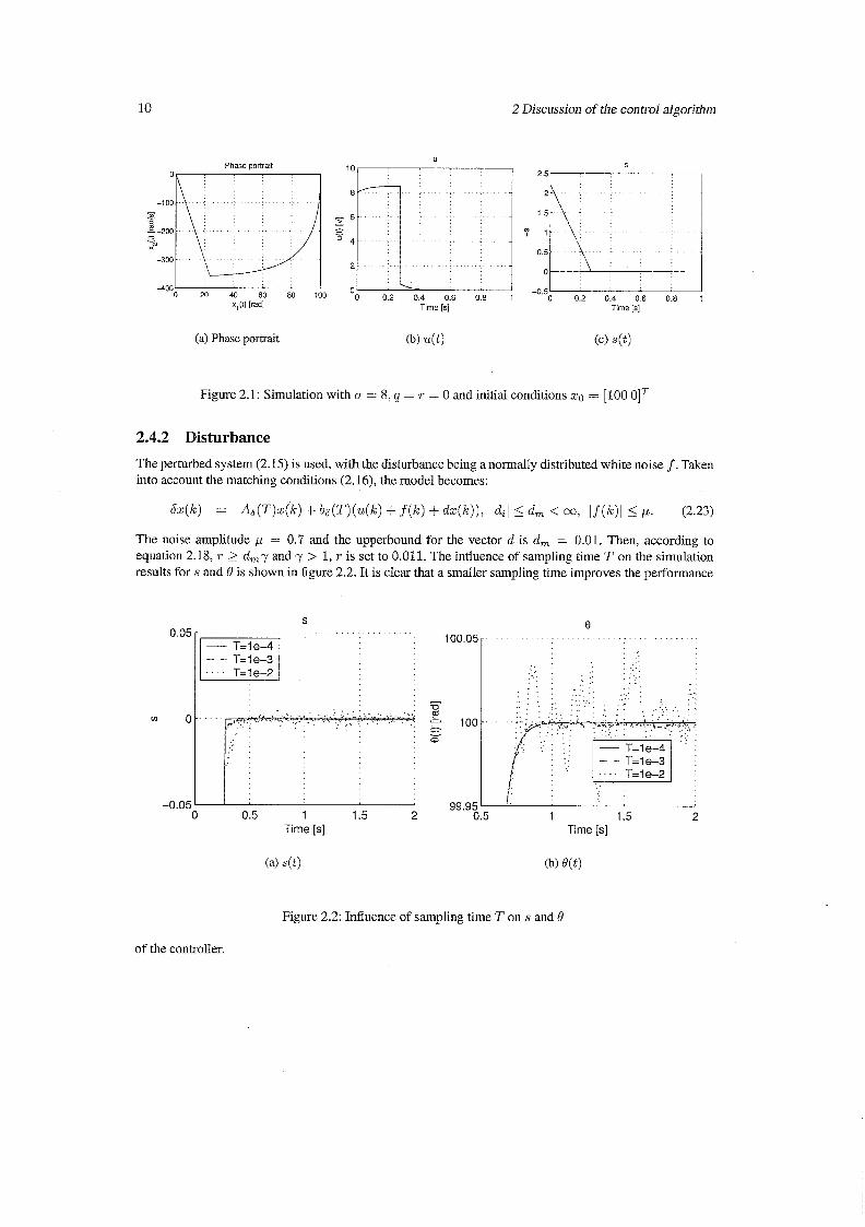
The goal of this project was to confront performance of the discrete-time SMC with the results shown in [14] and [15]. For a good comparison, the same reference trajectory is used, a so-called letter-writing trajectory. The robot has to perform the writing task shown in figure 3.1. The reference trajectory is such that this trajectory is followed in 10 seconds.

(a) Motion of the tip of the third joint (b) Joint motions

1 3 -

Joint 1

Figure 3.1 : Writing task

3.2 Identification

- Joint 2

1.-

A decoupling input-output linearizing controller is already implemented in the experimental setup [14], which yields for each joint the following input-output relation:

2

5 I c .- 0 + .- 8 0 - a

0.9

0.8

.$ 0.7 m L. 0.6

0.5

with 4; the acceleration of the joint, J a constant equal to 1, and u the control input. To check whether this model is valid, an experiment is done. In this experiment, the relevant joint is moving with constant speed,

-

- -

-

-

- - 1

-2

0.4

0.3 -0.4 -0.2 0 0.2 0.4 0 2 4 6 8 10

x-axis Time [s]

-

12 3 Implementation on the RRR-robot

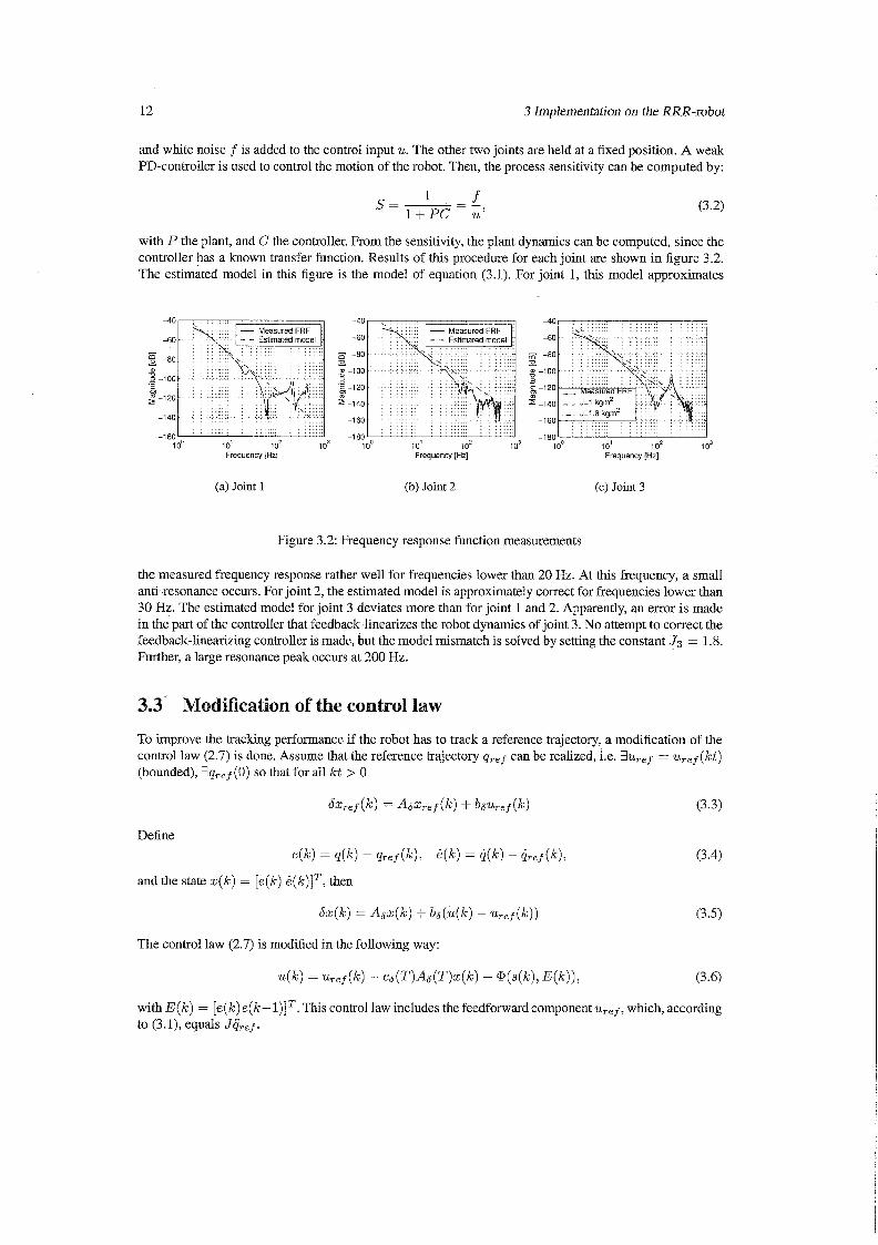
and white noise f is added to the control input u. The other two joints are held at a fixed position. A weak PD-controller is used to control the motion of the robot. Then, the process sensitivity can be computed by:

with P the plant, and C the controller. From the sensitivity, the plant dynamics can be computed, since the controller has a known transfer function. Results of this procedure for each joint are shown in figure 3.2. The estimated model in this figure is the model of equation (3.1). For joint 1, this model approximates

Frequency [Hz] Frequency [Hz]

. . . . . . . . . . . . . . . . . . . . . . . . . . .. -180

. . . . . . . . . . . . . . . . . . . .

1 o0 10' 1 02 1 o3 Frequency [Hz]

(a) Joint 1 (b) Joint 2 (c) Joint 3

Figure 3.2: Frequency response function measurements

the measured frequency response rather well for frequencies lower than 20 Hz. At this frequency, a small anti-resonance occurs. For joint 2, the estimated model is approximately correct for frequencies lower than 30 Hz. The estimated model for joint 3 deviates more than for joint 1 and 2. Apparently, an error is made in the part of the controller that feedback-linearizes the robot dynamics of joint 3. No attempt to correct the feedback-linearizing controller is made, but the model mismatch is solved by setting the constant J3 = 1.8. Further, a large resonance peak occurs at 200 Hz.

3.3. Modification of the control law

To improve the tracking performance if the robot has to track a reference trajectory, a modification of the control law (2.7) is done. Assume that the reference trajectory qTef can be realized, i.e. 3uTef = uref ( k t ) (bounded), 3qref(0) so that for all k t > 0

Define

e ( k ) = q(k) - qTef(k), e ( k ) = 4 ( k ) - qTe f ( k ) ,

and the state x ( k ) = [e(k) e(k)lT, then

bx (k ) = A6x(k ) + b & ( ~ ( k ) - uTef ( k ) )

The control law (2.7) is modified in the following way:

with E ( k ) = [e (k ) e (k- 1)IT. This control law includes the feedforward component u T e f , which, according to (3. I), equals JqTef .

3.4 Observer design 13

3.4 Observer design

The performance of a sliding mode controller depends strongly on the quality of the measurements of the available states. The presence of noise can cause the state to jump from one side of the sliding manifold to the other, which leads to chattering. Since noise-free measurements are impossible in practice, an observer is designed, which reconstructs the state from the measurement. The observer is designed using the model (3.1), with the uncertainty on the system equations and the measurement taken into account:

Here, v ( t ) represents the model error, which is modeled as white noise w ( t ) filtered by a single integrator. Due to this filtering, emphasis is placed on the estimation of the low-frequent behaviour, which is important due to the presence of Coulomb friction in the robot. y ( t ) represents the measured position error, and ~ ( t ) the measurement noise. The discrete equivalent of (3.7) is:

where

x ( k ) = [ 4 k ) 4 k ) l T , (3.9)

[ 1 T T 2 / 2 I , f l r i l T 2 / 2 ] , g ( T ) = [ T r 2 ] , c = [ l ~ ~ 1 6 0 0 1 . (3.10)

A Kalman observer provides an optimal reconstruction of the state in the presence of the modeling uncertainty and the measurement noise:

where % denotes the updated estimate of all states and K the optimal Kalman gain, as computed by the MATLAB-routine dlqe. Each time step, the estimate is updated based on the difference between the measured and the predicted error. In the experimental setup, a time delay of approximately two time steps is present. Therefore, this time delay is compensated by extending the observer state with two states e (k -2 ) and e(k - I ) , and treat the current measurement as e(k - 2). Then, the observer predicts e ( k ) , which can be used in the control law.

3.5 Tuning the controller parameters

3.5.1 Choice of a

The parameter a determines the behaviour inside the vicinity S. According to equations (2.12-2.14), the parameter a determines cg. When s is in the vicinity S of the sliding manifold, the reaching law equals +, and the control law is given by

This control law consists of a feedforward part and a linear state feedback. For small a T , cl approaches a , since

T -- T - cl = -6 = a + cg = [a 11. (3.13)

cg = [CI 1 1 ~ ~ ~ (T) [cl 11

14 3 Implementation on the RRR-robot

Further, for small T, the term A& in equation (3.12) is negligible, and the control law becomes

1 u = uref (k) + -[a l ] ~ ( k ) . T

(3.14)

The linear feedback actually is a PD-action, which approximately consists of the proportional action $ and the derivative action $. This means that the choice for a could be done by tuning a PD-controller on the measured frequency response of each joint. The smaller the sampling time T, the higher the feedback gain, and thus the smaller the influence of disturbances. The approximate gain $ is limited due to the high- frequent behaviour of the system, as can be seen in figure 3.2. Exciting the higher frequencies can result in chattering or even instability. Tuning a PD-controller on the measured frequency response is not possible in the current setup, since a Kalman filter is used to estimate the states. In this report, the Kalman filter is considered as a part of the controller. The transfer function of the Kalman filter with the controller is derived in appendix C, and shown in figure C.1. The choice for a will be done experimentally, because the combined transfer function of the controller and the Kalman filter is not very convenient for tuning. The performance criterion is the position tracking error, combined with the constraint that s should stay in S. The values for a, together with the corresponding P and D action, that give the best results are given in table 3.1. In all experiments, a sampling time T = 1 . is used. The values for joint 1 and 2 give very high feedback gains in the

Joint I ai I P I D 1 1 200 1 181. lo3 1 1091

Table 3.1: Final values of tuning parameter ai and corresponding PD-actions

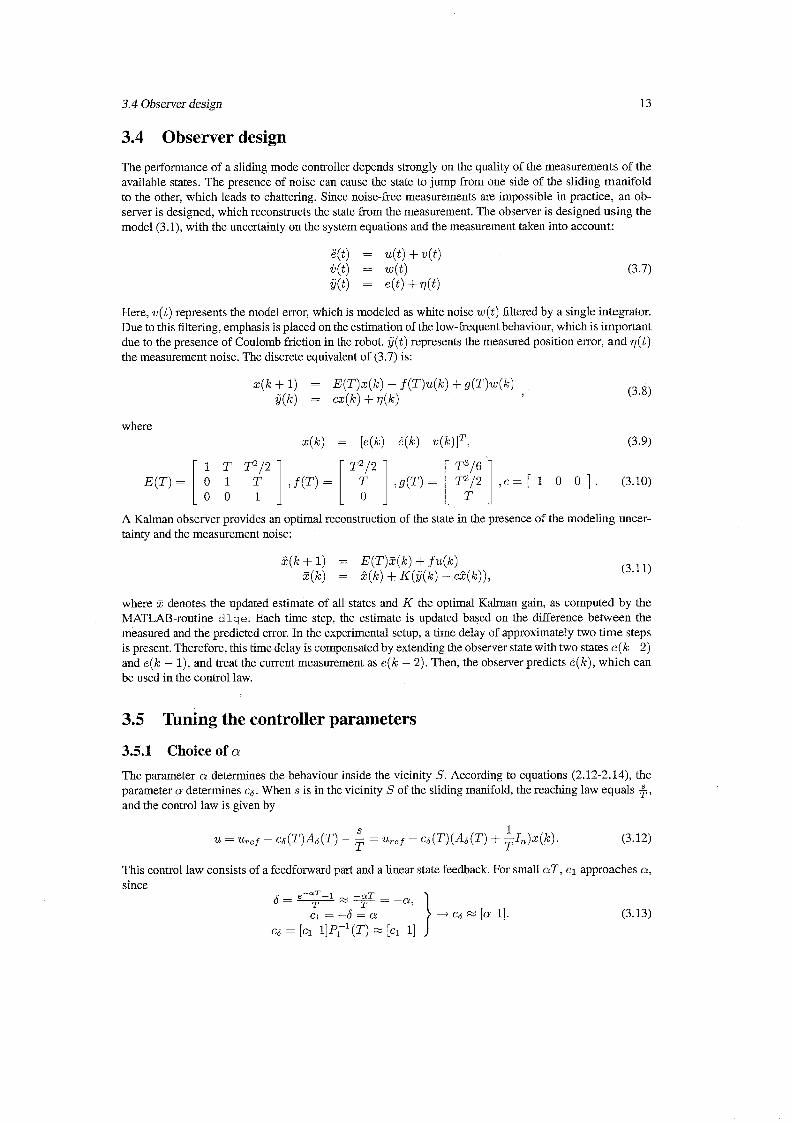
vicinity S, without leading to instability. The gains can become this high because the error predicted by the Kalman filter is used, which gives a phase lead. The maximum allowable value for a3 that yields a stable system in the vicinity S is much lower. Using the controller transfer as calculated in appendix C, the open loop transfer of each joint can be calculated. These are given in figure 3.3. From this figure, it

. , ....... >

. . . .. . . . . . . . . . . -1 00 . . . . . .. . . . .. ... . . . .. .

1 00 10' 1 o2 1 o3 1 o0 10' 1 o2 1 o3 I 00 10' 1 oZ 1 o3 Frequency [Hz] Frequency [Hz] Frequency [Hz]


Figure 3.3: Open loop transfers for each joint

can be concluded that the phase margins for joint 1 and 2 are very small. This doesn't lead to instability, because the controller switches to another mode if the switching function s leaves the vicinity S. From figure 3.3 (c), it can be argued that the gain of the controller for joint 3 could be raised. However, this lead to chattering during the experiments. The reason for this apparent contradiction is that the large resonance peak is amplified with a high control gain, and thus easily excites vibrations and consequently leads to control chattering.

3.5 Tuning the controller parameters

3.5.2 Choice of a, q and r

The parameters a, q and r determine the behaviour in the reaching phase, and according to equation (2.19), the width of the vicinity S. The width of the vicinity S is mostly determined by a. The parameters q and r have less influence on the width, but are useful for finetuning. To guarantee stability, a has to be larger than the model uncertainty. This model uncertainty is estimated online in the Kalman filter with the parameter v. Table 3.2 gives the maximum of the estimated model uncertainty for each joint, and the chosen value for n. The parameter r increases the width of the vicinity S when the error increases, so that s stays in S. This is especially useful in the parts of the trajectory with a high-frequent content, when the model is not very accurate. The parameter q is important for a fast response in the reaching phase. The experimentally determined values of the parameters q and r are also listed in table 3.2.

Table 3.2: Model uncertainty and final tuning parameters

3 Lmplementation on the RRR-robot

Chapter 4

Results

4.1 Results of the sliding mode controller

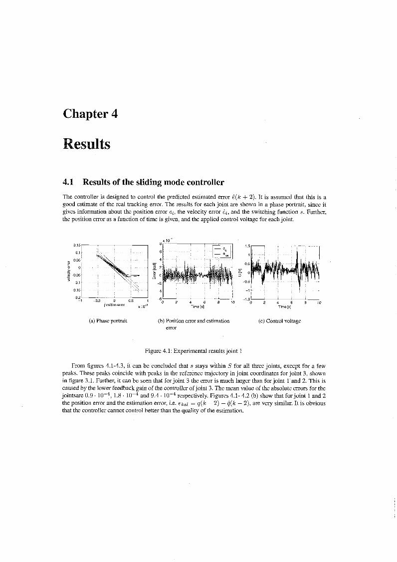
The controller is designed to control the predicted estimated error d(k + 2). It is assumed that this is a good estimate of the real tracking error. The results for each joint are shown in a phase portrait, since it gives information about the position error e,, the velocity error e,, and the switching function s. Further, the position error as a function of time is given, and the applied control voltage for each joint.

position error 10-3 Time Is]

(a) Phase portrait (b) Position error and estimation error

-1 I -1 5

0 2 4 6 8 1 0 Time [s]

(c) Control voltage

Figure 4.1: Experimental results joint 1

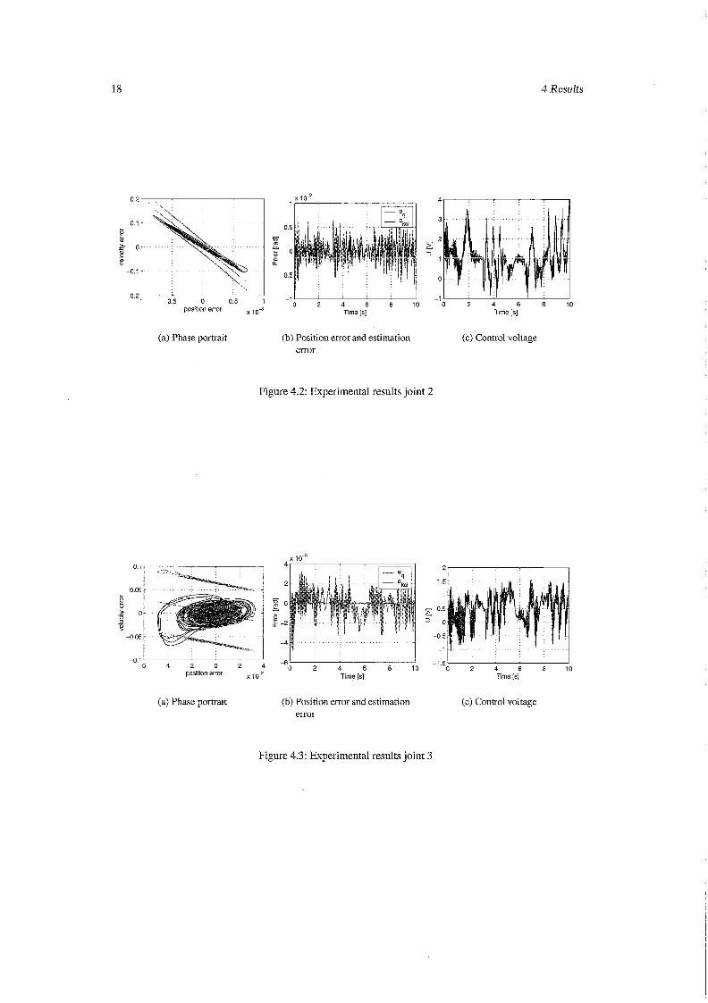
From figures 4.1-4.3, it can be concluded that s stays within S for all three joints, except for a few peaks. These peaks coincide with peaks in the reference trajectory in joint coordinates for joint 3, shown in figure 3.1. Further, it can be seen that for joint 3 the error is much larger than for joint 1 and 2. This is caused by the lower feedback gain of the controller of joint 3. The mean value of the absolute errors for the jointsare 0.9 . lop4, 1.8 . lop4 and 9.4 . respectively. Figures 4.1- 4.2 (b) show that for joint 1 and 2 the position error and the estimation error, i.e. ek,l = q(k - 2) - G(k - 2), are very similar. It is obvious that the controller cannot control better than the quality of the estimation.

4 Results

4

3

2 - e 3

0

-1 -05 O O5 -lo 2 4 6 8 10 0 2 4 6 8 10

posttlon enor 0* Tme [s] T~me [s]

(a) Phase portrait (b) Position error and estimation (c) Control voltage error


x lo3 0.1

0.05 0

0,

2 0 0 - ? -0.05

-0.1 -6 -4 -2 0 2 4 -60 2 4 6 8 10

position error 0 2 4 6 8 1 0

Time [s] Time [s]

(a) Phase portrait (b) Position error and estimation (c) Control voltage error


4.1 Results of the sliding mode controller

4.1.1 Discussion

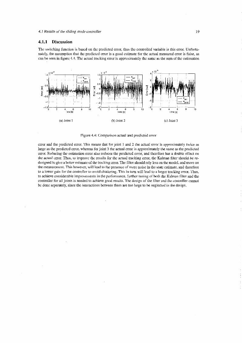
The switching function is based on the predicted error, thus the controlled variable is this error. Unfortu- nately, the assumption that the predicted error is a good estimate for the actual measured error is false, as can be seen in figure 4.4. The actual tracking error is approximately the same as the sum of the estimation

x lo* 1.5

1 2

0.5 fi m o

7 0 - - b

? -0.5 5 -2 -1

-4 -1.5

-2 -6 0 2 4 6 8 1 0 0 2 4 6 8 1 0 0 2 4 6 8 1 0

Time [s] Time [s] Time [s]


Figure 4.4: Comparison actual and predicted error

error and the predicted error. This means that for joint 1 and 2 the actual error is approximately twice as large as the predicted error, whereas for joint 3 the actual error is approximately the same as the predicted error. Reducing the estimation error also reduces the predicted error, and therefore has a double effect on the actual error. Thus, to improve the results for the actual tracking error, the Kalman filter should be re- designed to give a better estimate of the tracking error. The filter should rely less on the model, and more on the measurement. This however, will lead to the presence of more noise in the state estimate, and therefore to a lower gain for the controller to avoid chattering. This in turn will lead to a larger tracking error. Thus, to achieve considerable improvements in the performance, further tuning of both the Kalman filter and the controller for all joints is needed to achieve good results. The design of the filter and the controller cannot be done seperately, since the interactions between them are too large to be neglected in the design.

20 4 Results

4.2 Comparison with H, controller

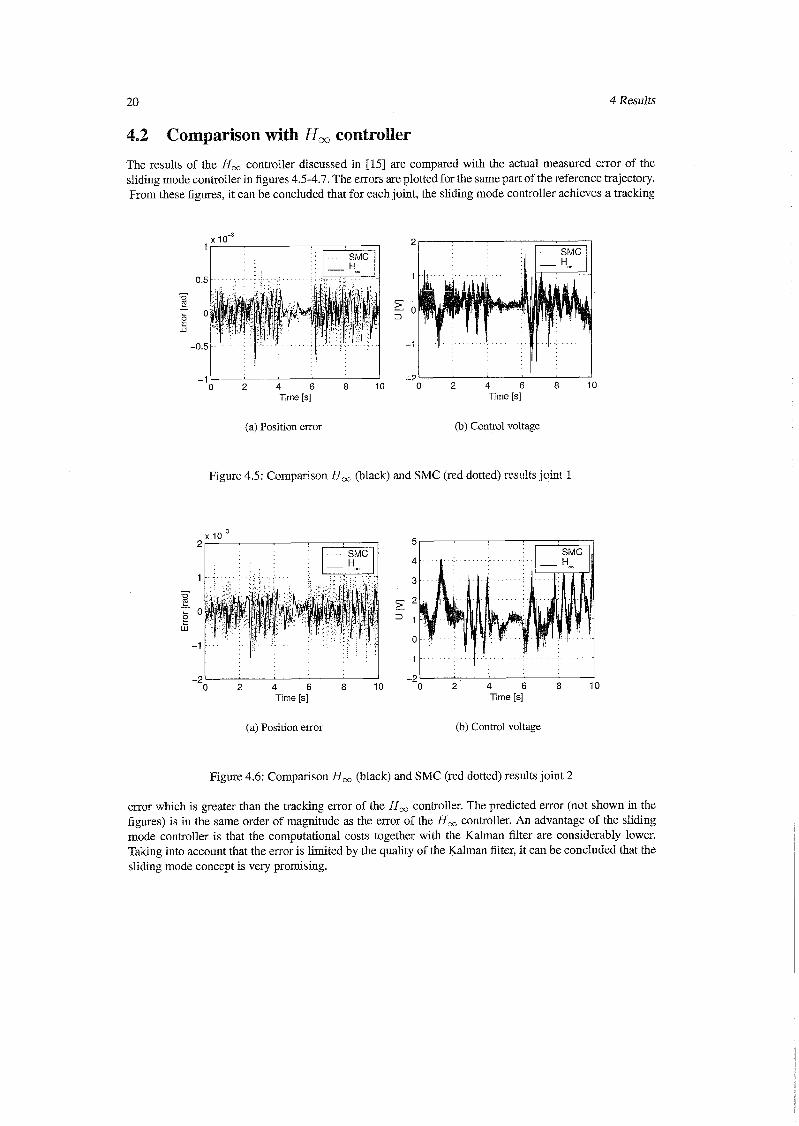
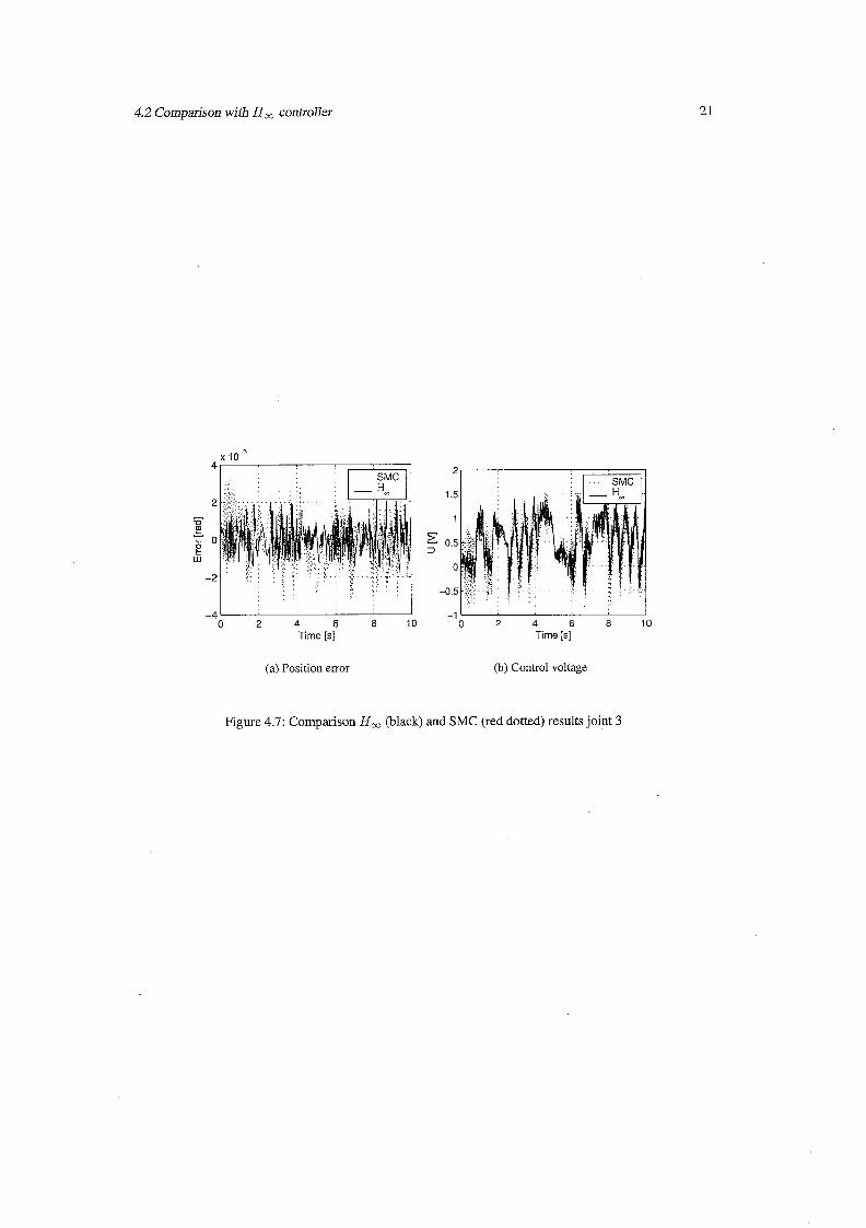
The results of the H , controller discussed in [I51 are compared with the actual measured error of the sliding mode controller in figures 4.5-4.7. The errors are plotted for the same part of the reference trajectory. From these figures, it can be concluded that for each joint, the sliding mode controller achieves a tracking

-1 1 0 2 4 6 8 1 0

Time [s]

I . -21 I

0 2 4 6 8 1 0 Time [s]

(a) Position error (b) Control voltage

Figure 4.5: Comparison H , (black) and SMC (red dotted) results joint I

Time [s] Time [s]


Figure 4.6: Comparison H , (black) and SMC (red dotted) results joint 2

error which is greater than the tracking error of the H , controller. The predicted error (not shown in the figures) is in the same order of magnitude as the error of the H , controller. An advantage of the sliding mode controller is that the computational costs together with the Kalman filter are considerably lower. Taking into account that the error is limited by the quality of the Kalman filter, it can be concluded that the sliding mode concept is very promising.

4.2 Comparison with H , controller

I . . . -4 1 I

0 2 4 6 8 1 0 0 2 4 6 8 1 0 Time [s] Time [s]


Figure 4.7: Comparison H , (black) and SMC (red dotted) results joint 3

4 Results

Chapter 5

endations

In this report, a discrete time sliding mode algorithm is designed and validated on the experimental setup of a RRR-robot. The design of the controller in the sliding mode can be done by tuning a PD-controller on the measured frequency response. The performance in terms of the tracking error is less than with an H, controller, but the computational costs for the control effort are considerably lower. The tracking performance is limited by the quality of the Kalman filter and high-frequent model uncertainties. Further tuning of both Kalman filter and controller is needed to achieve a performance at the same level as the H, controller.

5 Conclusions & Recommendations

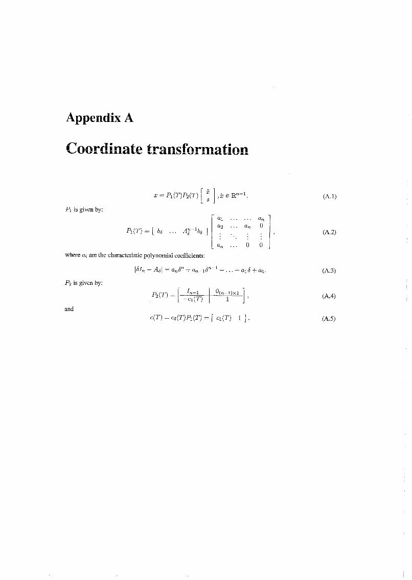
Appendix A

sformati

Pl is given by: [ a 1 ... ... an 1

a2 . . . a, 0 PI ( T ) = [ bs . . . A;-lb6 ] . . >

where ai are the characteristic polynomial coefficients:

P2 is given by:

A Coordinate transformation

Appendix B

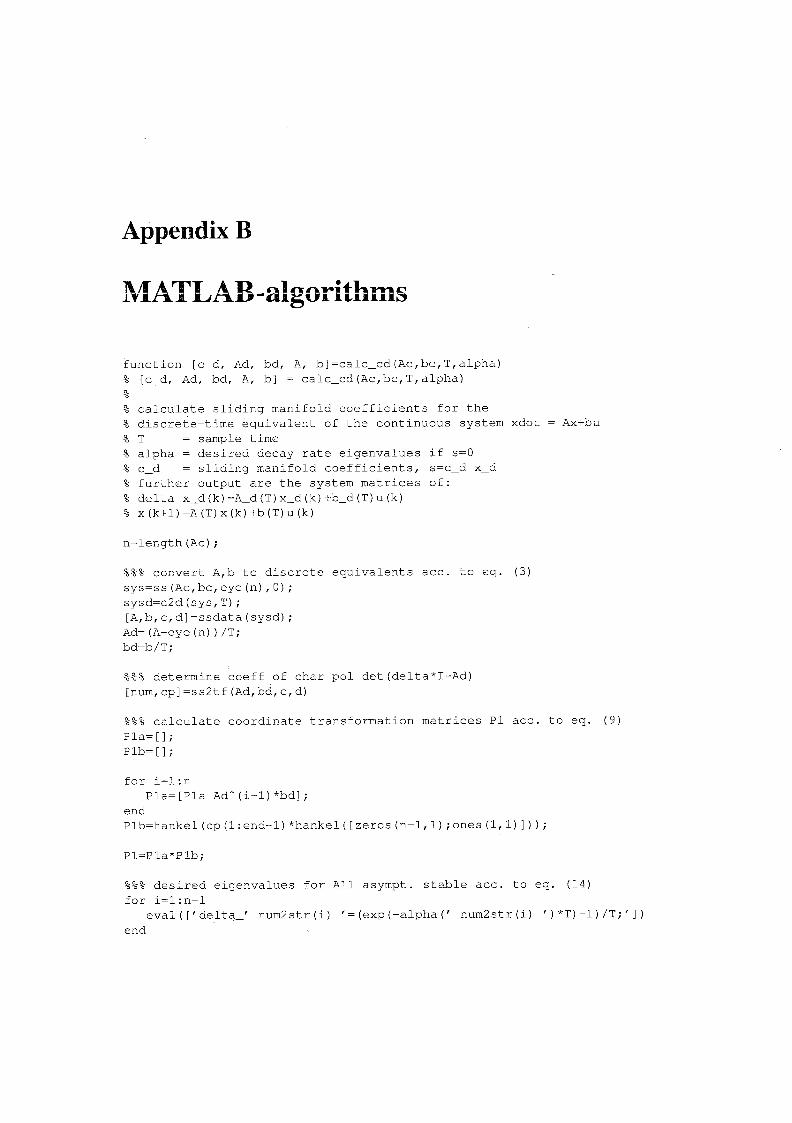
function [c-d, Ad, bd, A, b] =talc-cd (Ac, bc, T, alpha) % [c-d, Ad, bd, A, b] = calc-cd(Ac,bc,T,alpha) 3

% calculate sliding manifold coefficients for the % discrete-time equivalent of the continuous system xdot = Ax+bu % T = sample time % alpha = desired decay rate eigenvalues if s=O % c-d = sliding manifold coefficients, s=c-d x-d % further output are the system matrices of: % delta x-d (k) =A-d (T) x-d (k) +b-d (T) u (k) % x (k+l) =A (T) x (k) +b (T) u (k)

n=length (Ac) ;

3 3 3 ... convert A,b to discrete equivalents acc. to eq. (3) sys=ss (Ac, bc, eye (n) ,0) ; sysd=c2d (sys, T) ; [A, b, c, dl =ssdata (sysd) ; Ad= (A-eye (n) ) /T; bd=b/T;

3 % ~ .,, determine coeff of char pol det(deltakI-Ad) [num, cp] =ss2tf (Ad,bd, c, d)

3 3 3 ... calculate coordinate transformation matrices P1 acc. to eq. (9) Pla= [I ; Plb=[] ;

for i=l:n Pla= [Pla Ad- (i-1) *bd] ;

end Plb=hankel (cp (1:end-1) *hankel ([zeros (n-1,l) ;ones (1,l) ] ) ) ;

~ 3 % ... desired eigenvalues for All asympt. stable acc. to eq. (14) for i=l:n-1

eval ( ['delta-' num2str (i) '= (exp (-alpha ( ' num2str (i) ' ) *T) -1) /T; ' ] ) end

5~3% ,,, calculate elements of cl acc. to eq. (15)

cl=[] ;

% calculate product function in eq. (15) syms delta

p=l ; for j=l:n-1

eval( ['p= (delta-delta-' num2str (j) ' ) *p; ] )

end

% calculate elements c-i of vector cl for i=l:n-1

eval ( [ ' c-' num2str (i) '=l/factorial (i-1) *diff(p, i-1) ; ] )

eval ( [ ' c-' num2str (i) '=subs (c-' num2str (i) ' ,delta, 0) ; ' ] )

eval (['cl=[cl c-' num2str (i) ' 1 ;' ] ) end

% % % o o o calculate vector c-d, defining sliding manifold, acc to eq. (16)

c-d=double ( [cl l] *inv (PI) ) ;

Appendix C

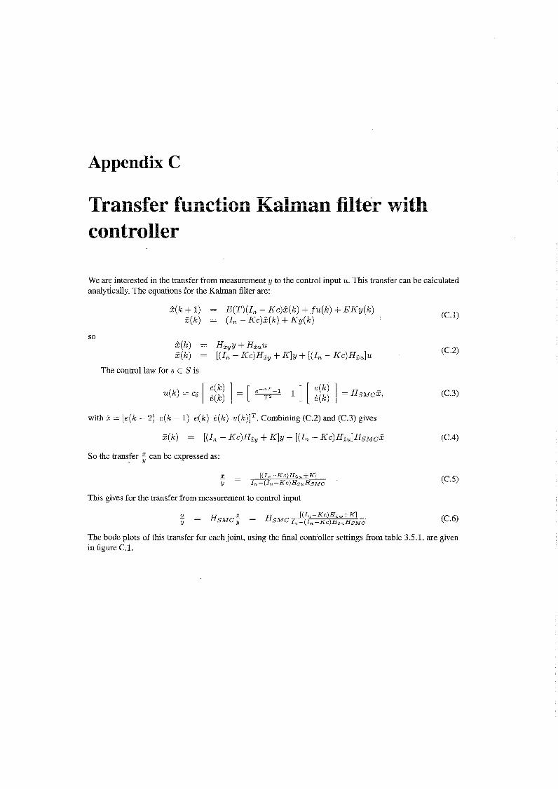
We are interested in the transfer from measurement y to the control input u. This transfer can be calculated analytically. The equations for the Kalman filter are:

The control law for s E S is

with LF = [e(k - 2) e(k - 1) e ( k ) e ( k ) v (k) lT . Combining (C.2) and (C.3) gives

So the transfer can be expressed as:

This gives for the transfer from measurement to control input

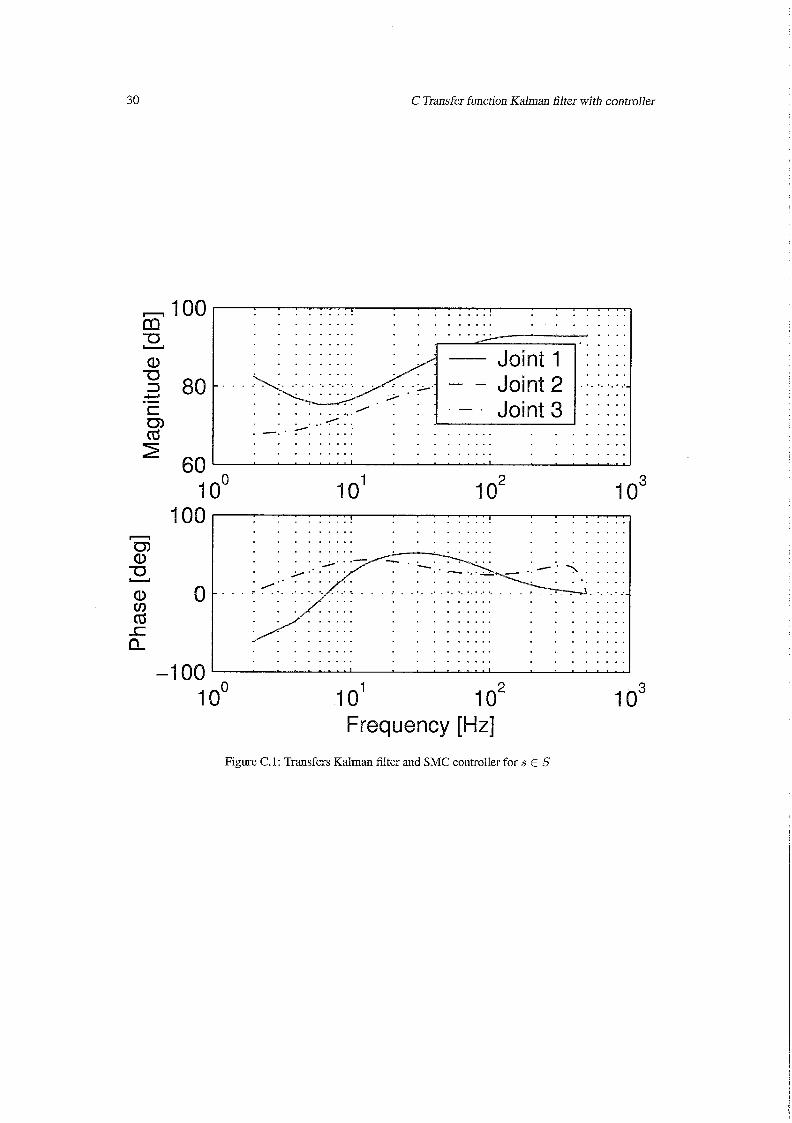
The bode plots of this transfer for each joint, using the final controller settings from table 3.5.1, are given in figure C. 1.

C Transfer function Kalman filter with controller

Frequency [Hz]

Figure C.1: Transfers Kalman filter and SMC controller for s E S

[I] J.Y. Hung, W. Gao, J.C. Hung, "Variable Structure Control: A Survey," IEEE Transactions On Indus- trial Electronics, Vol. 40, No. 1, pp. 2-22, February 1993.

[2] V.I. Utkin, "Sliding Mode Control Design Principles and Applications to Electric Drives," IEEE Transactions On Industrial Electronics, Vol. 40, No. 1, pp. 23-36, February 1993.

[3] W. Gao, J.C. Hung, "Variable Structure Control of Nonlinear Systems: A New Approach," IEEE Transactions On Industrial Electronics, Vol. 40, No. 1, pp. 45-55, February 1993.

[4] c. MilosavljeviC, "General Conditions for the Existence of a Quasi-sliding Mode on the Switching Hyperplane in Discrete Variable Structure Systems," Automatic Remote Control, Vol. 46, pp. 307-3 14, 1985.

[5] W. Gao, Y. Wang, A. Homaifa, "Discrete-time Variable Structure Control Systems," IEEE Transac- tions on Industrial Electronics, Vol. 42, NO. 2, pp. 117-122, April 1995.

[6] G. Golo, c. MilosavljeviC, "Parabolic and Triangular Wave Oscillator With Sliding Mode," Electronic Letters, Vol. 32, No. 17, pp. 1535-1536, August 1996.

[7] G. Golo, C. MilosavljeviC, "Two-phase Triangular Wave Oscillator Based on Discrete-time Sliding Mode Control," Electronic Letters, Vol. 33, No. 22, pp. 1838-1839, October 1997.

[8] G. Golo, C. MilosavljeviC, "Robust Discrete-time Chattering Free Sliding Mode Control," Systems & Control Letters, Vol. 41, pp. 19-28, 2000.

[9] A.M. van Beek, RRR-robot: Instruction manual, WFW report 98.012, Eindhoven University of Tech- nology, Faculty of Mechanical Engineering, Section Systems & Control, March 1998.

[lo] A.M. van Beek, RRR-robot: Design of an Industrial-like Test Facility for Nonlinear Robot Control, WFW report 98.014, Eindhoven University of Technology, Faculty of Mechanical Engineering, Sec- tion Systems & Control, May 1998.

[1 11 D. KostiC, R. Hensen, B. de Jager, M. Steinbuch, "Modeling and Identification of an RKR-robot," in Trans. of IEEE Conference On Decision and Control, pp. ,Orlando, Florida, December 4-7,2001.

[12] D. KostiC, R. Hensen, B. de Jager, and M. Steinbuch, "Closed-form Kinematic and Dynamic Models of an Industrial-like RRR Robot," in Trans. IEEE International Conference on Robotics and Automa- tion, pp. 1309-1314, Washington D.C., USA, May, 2002.

[13] A. den Hamer, "Adapive Control of RRK-manipulators," report following 6-weeks trainingship at DCT group in 2002.

[14] D. KostiC, R. Hensen, B. de Jager, and M. Steinbuch, "Experimentally Supported Control Design for a Direct Drive Robot," in Trans. IEEE Conference on Control 186-191, Glasgow, United Kingdom, September, 2002.

[15] D. KostiC, B. de Jager, and M. Steinbuch, "Control Design for Robust Performance of a Direct-drive Robot," accepted for IEEE Control Appl. Conf., Istanbul, June 23-25,2003.

Documents

Discrete-time Sliding Mode Control of the RRR-robot