Discretizations in Isogeometric Analysis of Navier-Stokes Flow

Peter Nørtoft Nielsena,b,∗, Allan Roulund Gersborgb,1, Jens Gravesena, Niels LeergaardPedersenb

aDTU Mathematics, Technical University of Denmark, Matematiktorvet 303S, DK-2800 Kgs. Lyngby, DenmarkbDTU Mechanical Engineering, Technical University of Denmark, Nils Koppels All 404, DK-2800 Kgs. Lyngby,

Denmark

Abstract

This paper deals with isogeometric analysis of the 2-dimensional, steady state, incompress-ible Navier-Stokes equation subjected to Dirichlet boundary conditions. We present a detaileddescription of the numerical method used to solve the boundary value problem. Numerical inf-sup stability tests for the simplified Stokes problem confirmthe existence of many stable dis-cretizations of the velocity and pressure spaces, and in particular show that stability may beachieved by means of knot refinement of the velocity space. Error convergence studies for thefull Navier-Stokes problem show optimal convergence ratesfor this type of discretizations. Fi-nally, a comparison of the results of the method to data from the literature for the the lid-drivensquare cavity for Reynolds numbers up to 10,000 serves as benchmarking of the discretizationsand confirms the robustness of the method.

Keywords:isogeometric analysis, fluid mechanics, Navier-Stokes flow, inf-sup stability, lid-driven squarecavity

1. Introduction

Isogeometric analysis unites the power to solve complex engineering problems from finiteelement analysis (FEA) with the ability to smoothly represent complicated shapes in very fewdegrees of freedom from computer aided design (CAD) [1, 2]. Within recent years, isogeomet-ric analysis has been applied to various flow problems and proved its value within the field offluid mechanics. Some of the first studies were on steady-state incompressible Stokes flow inthe benchmarking lid-driven square cavity [3]. Subsequentanalysis of the full time dependentNavier-Stokes equations using the isogeometric method hasshown its advantages both in termsof continuity of state variables [4] and the ability to accurately represent complicated dynamicflow domains [5]. Benchmarking of the method for the turbulent Taylor-Couette flow shows verynice performance of the method [6].

∗Corresponding author.Email addresses: p.n.nielsen@mat.dtu.dk (Peter Nørtoft Nielsen),agersborg.hansen@gmail.com (Allan

Roulund Gersborg),j.gravesen@mat.dtu.dk (Jens Gravesen),nlp@mek.dtu.dk (Niels Leergaard Pedersen)1Present address:Burmeister & Wain Energy A/S, Lundtoftegårdsvej 93A, DK-2800 Kgs. Lyngby, Denmark

Preprint submitted to Computer Methods in Applied Mechanics and Engineering 17 June, 2011

An important issue in the analysis of the mixed formulation of the governing equations forfluids is the stability of the element, or discretization, used to approximate the state variables.The first stable B-spline discretization for the Stokes problem was proposed in [3]. Recently, twomore families of stable B-spline discretizations were identified in [7], thereby further emphasiz-ing how easily high degrees of continuity may be achieved in isogeometric analysis. Mathemat-ical proofs of the stability of a range of discretizations have very recently been made [8, 9].

The aim of this paper is threefold. Firstly, we wish to extendthe list of stable B-splinediscretizations for the 2D steady state, incompressible Stokes problem. Secondly, we wish applythe method to the non-linear 2D steady state, incompressible Navier-Stokes problem and examinehow these discretizations perform in terms of error convergence based on a flow problem withan analytical solution. Finally, the benchmarking lid-driven square cavity will be analysed andthe results of the discretizations compared to data from theliterature.

The outline of the paper is as follows. Section 2 presents theequations that govern problemsin fluid mechanics, and section 3 outlines how the problem is solved using isogeometric analysis.In section 4 we perform a numerically test of different isogeometric discretizations in terms ofstability, and an error convergence study for these discretizations is presented in section 5. Finallyin section 6, a comparison of the discretizations against results from the literature is presentedfor the benchmarking lid-driven square cavity.

2. Boundary Value Problem

We consider a fluid contained in the domainΩ with boundaryΓ ≡ ∂Ω, see figure 1. We as-sume the fluid to be a viscous, incompressible, isothermal, Newtonian fluid, and we furthermoreassume it to be stationary. The fluid is then governed by:

−µ∆u + ρu · ∇u + ∇p − ρ f = 0 inΩ (1a)

∇ · u = 0 inΩ (1b)

Equation (1a) is the the steady-state Navier-Stokes equation, expressing conservation of mo-mentum for the fluid and written in the primitive variablesp andu, wherep is pressure andu = (u1, u2) is the fluid velocity. The quantitiesρ, µ and f denote the density, dynamic viscosityand additional body forces acting on the fluid, respectively. Equation (1b) is the incompressibilitycondition, and it expresses conservation of mass.

We assume the velocityu to be prescribed along the bondaryΓ, and we take the mean pressureto be zero:

u = uD onΓ (1c)∫∫

Ω

p dA = 0 (1d)

whereD in equation (1c) stands for Dirichlet. Other boundary conditions, such as Neumannboundary conditions, could also be considered but have beenleft out for simplicity.

Numerical methods for solving Navier-Stokes equation (1a)can employ different formula-tions of the equation. The main results of the present study are based on theconvective for-mulation. Comparisons to theskew-symmetric formulation are also made, while therotational

2

formulation is left out to avoid the introduction of stabilization [10]. The two formulations differin their treatment of the non-linear inertial termu · ∇u:

(u · ∇)u or (u · ∇)u +12∇ · u. (2)

Compared to the convective formulation, the skew-symmetric formulation additionally involvesthe divergence of the velocity field. Even though these formulations on a continous level areexactly equivalent, due to the incompressibility condition (1b), this is not the case on a discretelevel, and therefore the numerical solutions might differ.

3. Isogeometric Method

Equations (1) together comprise thestrong form of the boundary value problem that governsthe state of the fluid. We use NURBS-based isogeometric analysis built on Galerkin’s method tosolve the problem numerically. This section outlines the procedure. See also [2, 11, 12].

3.1. Geometry Parametrisation

The physical domainΩ is parametrised using NURBS, Non-Uniform Rational B-splines. Tomake the text self-contained, we very briefly revise the basic concepts of B-splines and NURBSin the following. For a more in-depth treatment of this subject, we refer the reader to e.g. [13].

To define univariate B-splines we choose a polynomial degreeq ∈ N and a knot vectorΞ = ξ1, . . . , ξm with ξi ∈ R for i = 1, . . . ,m. For simplicity, we assume the parametric domainξ ∈ [0, 1], and that the knot vector is open such that the boundary knots have multiplicityq + 1with ξ1 = ξ2 = . . . = ξq+1 = 0 andξm = ξm−1 = . . . = ξm−q = 1. The univarite B-splinesNq

i : [0; 1]→ R are defined recursively as

N0i (ξ) =

1 if ξi ≤ ξ < ξi+1

0 otherwise(3a)

for q = 0, and

Nqi (ξ) =

ξ − ξiξi+q − ξi

Nq−1i (ξ) +

ξi+q+1 − ξξi+q+1 − ξi+1

Nq−1i+1 (ξ) (3b)

for q = 1, 2, . . ..The bivariate tensor product B-splinesPq,r

i, j : [0, 1]2 → R are defined from two polynomialdegreesq andr and two knot vectorsΞ = ξ1, . . . , ξm andΦ = φ1, . . . , φn:

Pq,ri, j (ξ1, ξ2) = Nq

i (ξ1)Mrj(ξ2), (4)

whereNqi is the ith univariate B-spline with degreeq and knot vectorΞ in the first parametric

dimensionξ1 as defined in equation (3), andMrj is the jth univariate B-spline with degreer and

knot vectorΦ in the second parametric dimensionξ2.The bivariate NURBSRq,r

i, j : [0, 1]2 → R are defined from theNM bivariate B-splines inequation (4) and the weightsW = w1,1, . . . ,wN,M with wi, j ∈ R for i = 1, . . . ,N and j =1, . . . ,M:

Rq,ri, j (ξ1, ξ2) =

wi, jPq,ri, j∑N

k=1∑M

l=1 wk,lPq,rk,l

(5)

3

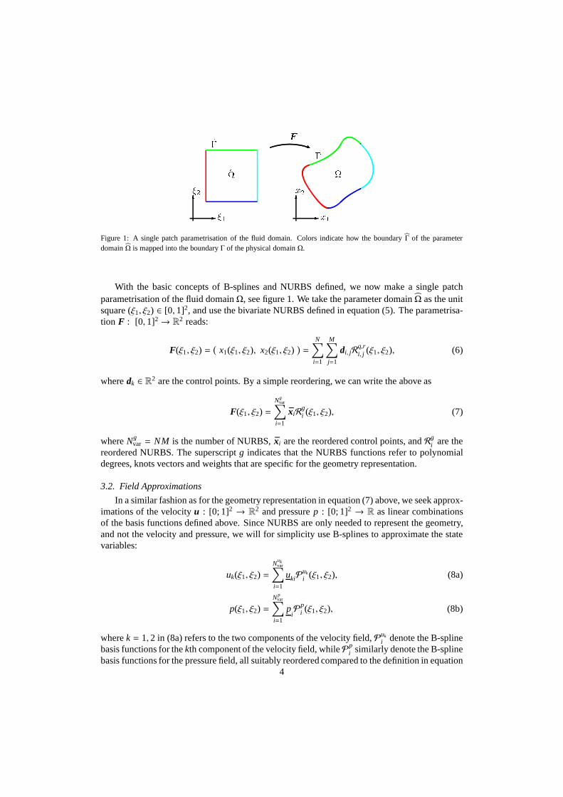
Figure 1: A single patch parametrisation of the fluid domain.Colors indicate how the boundaryΓ of the parameterdomainΩ is mapped into the boundaryΓ of the physical domainΩ.

With the basic concepts of B-splines and NURBS defined, we nowmake a single patchparametrisation of the fluid domainΩ, see figure 1. We take the parameter domainΩ as the unitsquare (ξ1, ξ2) ∈ [0, 1]2, and use the bivariate NURBS defined in equation (5). The parametrisa-tion F : [0, 1]2→ R

2 reads:

F(ξ1, ξ2) =(

x1(ξ1, ξ2), x2(ξ1, ξ2))=

N∑

i=1

M∑

j=1

di, jRq,ri, j (ξ1, ξ2), (6)

wheredk ∈ R2 are the control points. By a simple reordering, we can write the above as

F(ξ1, ξ2) =Ng

var∑

i=1

xiRgi (ξ1, ξ2), (7)

whereNgvar = NM is the number of NURBS,xi are the reordered control points, andRg

i are thereordered NURBS. The superscriptg indicates that the NURBS functions refer to polynomialdegrees, knots vectors and weights that are specific for the geometry representation.

3.2. Field Approximations

In a similar fashion as for the geometry representation in equation (7) above, we seek approx-imations of the velocityu : [0; 1]2 → R

2 and pressurep : [0; 1]2 → R as linear combinationsof the basis functions defined above. Since NURBS are only needed to represent the geometry,and not the velocity and pressure, we will for simplicity useB-splines to approximate the statevariables:

uk(ξ1, ξ2) =N

ukvar∑

i=1

ukiPuki (ξ1, ξ2), (8a)

p(ξ1, ξ2) =N p

var∑

i=1

piPp

i (ξ1, ξ2), (8b)

wherek = 1, 2 in (8a) refers to the two components of the velocity field,Puki denote the B-spline

basis functions for thekth component of the velocity field, whilePpi similarly denote the B-spline

basis functions for the pressure field, all suitably reordered compared to the definition in equation4

(4). They refer to separate sets of polynomial degrees and knot vectors that are in general not thesame.Nuk

var andNpvar are the number of velocity and pressure basis functions, while uk andp are

the unknown control variables for the velocity and pressurethat are to be determined.The velocity and pressure fields in equations (8) are defined in parameter space, while the

governing equations (1) are formulated in physical space. To evaluate the fields in physicalspace, the inverse of the geometry parametrisationF is used; the pressurep : Ω → R over thephysical domain is computed asp F−1, and the velocityu : Ω→ R

2 over the physical domainasu F−1. The Piola mapping could also be used to map the velocity [7],but since none ofthe examined discretizations are exactly divergent free, we take the simpler approach and mapeach velocity component as a scalar field. With abuse of notation, we use the same symbol forthe state variables both in parameter space and in physical space. Gradients in parameter space,

∇p =[∂p∂ξ1

∂p∂ξ2

]T, are easily evaluated using the field approximations in equation (8) and the

definition of B-splines in equation (4). Gradients in physical space,∇p =[∂p∂x1

∂p∂x2

]T, are related

to the gradients in parameter space by the formula:

∇p = JT∇p ⇐⇒ ∇p = J−T ∇p, (9)

whereJ is the Jacobian matrix of the geometry parametrisation:

J =

∂x1∂ξ1

∂x1∂ξ2

∂x2∂ξ1

∂x2∂ξ2

, (10)

which again is easily evaluated using the mapping in equation (7) and the definitions of NURBSin equation (5).

3.3. Boundary Conditions

For simplicity we impose the Dirichlet boundary conditionsin (1c)strongly as opposed to theweak enforcement suggested in [14, 15]. Hereby we avoid the need for definition of penalizationparameters which is favorable if a sequence of analysis withdifferent geometries is to performedas in shape optimization problems [16].

In general B-splines have compact support. This means that only a few of the velocity basisfunctionsPuk

i in equation (8a) have support onΓ. We can simply arrange the functionsPuk sothat the firstNuk

dof of these donot have support on the boundary, and the corresponding controlvariables of these are thus “degrees of freedom”, while the lastNuk

fix = Nukvar − Nuk

dof have supportonΓ, and the corresponding control variables are thus “fixed”:

uk(ξ1, ξ2) =

Nukdof∑

i=1

ukiPuki (ξ1, ξ2) +

Nukvar∑

i=Nukdof+1

ukiPuki (ξ1, ξ2). (11)

The strong imposition is done by directly specifying suitable values for these lastNuk

fix velocitycontrol variablesuki, so that the sum in equation (8a) approximates the specified valueuD in (1c).If uD lies within the function space spanned byPuk

i , the conditions are satisfied exactly; otherwisethey are only satisified in a least square sense.

For the pressure, we note that only the pressuregradient appears in the Navier-Stokes equa-tion (1a). The pressure is thus only determined up to an arbitrary constant, which is dealt with

5

by the specification of the mean pressure in equation (1d). Using the approximation in equation(8b), this gives rise to the following equation:

0 =∫∫

Ω

p dA =∫∫

Ω

N pvar∑

i=1

piPp

i (x1, x2) dx1 dx2

=

N pvar∑

i=1

pi

1 1∫∫

0 0

Ppi (ξ1, ξ2) det

(J)dξ1 dξ2 = pMT , (12)

wherep is the vector of pressure control variables,M the vector of integrals of pressure basisfunctions, andJ is given by (10). Since no pressure control variables needs to be fixed, we haveNp

dof = Npvar andNp

fix = 0.

3.4. Weak Form of the Governing EquationsThe governing equations (1) are cast into theirweak, or variational, form. For this we use

the (image in physical space of the) B-spline introduced above asweight functions for the gov-erning equations. We will use only the firstNuk

dof velocity basis functions, since these have nosupport on the fixed boundary. We multiply thekth component of the Navier-Stokes equation(1a) by an arbitrary weight functionPuk

i among these velocity basis functions, and the incom-pressibility equation (1b) by an arbitrary weight functionPp

j among the pressure basis functions,integrate the resulting equations overΩ, and then simplify using integration by parts. After somemanipulations we find the following weak form of the governing equations:

0 =∫∫

Ω

((µ∇Puk

i + ρPuki u) · ∇uk − (p∇Puk

i + ρPuki f ) · ek

)dx1 dx2 (13a)

0 =∫∫

Ω

Ppj (∇ · u) dx1 dx2 (13b)

for k = 1, 2, i = 1, . . . ,Nuk

dof and j = 1, . . . ,Npdof, and whereek is thekth unit vector.

3.5. Matrix EquationFinally, we insert the (image in physical space of the) approximations of the velocity and

pressure fields (8) into the weak form (13) of the governing equations, split the superpositions ofu into parts with support on the fixed boundary and parts without as in equation (11), exchangethe order of summation and integration, rearrange to get theunknown terms on the LHS andthe known terms on the RHS, and pull the integration back to parameter space using standardtransformation rules for multiple integrals along with equation (9). This gives:

M(U)︷ ︸︸ ︷K1 + C1(u) 0 −GT

10 K2 + C2(u) −GT

2G1 G2 0

U︷ ︸︸ ︷u1

u2

p

=

f1

f2

0

−

K⋆1 + C⋆1 (u) 0

0 K⋆2 + C⋆2 (u)G⋆1 G⋆2

[u⋆1u⋆2

]

︸ ︷︷ ︸F

, (14)

6

or simply M(U) U = F, with

Ki jk = µ

1 1∫∫

0 0

(J−T∇Puk

i

)·(J−T∇Puk

j

)det(J)dξ1 dξ2, (15a)

Ci jk(u) = ρ

1 1∫∫

0 0

Puki

(u(ul) ·

(J−T∇Puk

j

))det(J)dξ1 dξ2, (15b)

Gi jk =

1 1∫∫

0 0

Ppi

(J−T∇Puk

j

)· ek det

(J)dξ1 dξ2, (15c)

fik = ρ

1 1∫∫

0 0

Puki

(f · ek

)det(J)dξ1 dξ2, (15d)

Kk =[

Kk K⋆k] (

Nukdof × (N

ukdof+N

ukfix )), (15e)

Ck(u) =[

Ck(u) C⋆k (u)] (

Nukdof× (N

ukdof+N

ukfix )), (15f)

Gk =[

Gk G⋆k] (

N pdof ×(N

ukdof+N

ukfix )), (15g)

wherek = 1, 2, J is the Jacobian matrix in equation (10),u(u) is given by the approximationin equation (8),ek is thekth unit vector,u

T

k = [uT

k u⋆T

k ], and all starred quantities are given bythe boundary conditions.Kk is often called viscosity matrix,Ck convective matrix,Gk gradientmatrix, andfk force vector.

The integrals in equation (15) are evaluated using Gaussianquadrature. The necessary num-ber of quadrature pointsNG in each knot span is estimated from the relation ˜q = 2NG − 1, whereq is an estimate of the highest polynomial degree of the integrands. Since the integrands are ingeneral rational functions, we simply estimate ˜q as the sum of polynomial degrees of the numer-ator and the denominator. Using polynomial degree 2 for the geometry and 4 for the velocity andpressure, we estimate a polynomial degree of ˜q = 12 for the integrand ofC, and this dictates thatwe should use at leastNG = 7 quadrature points in each knot span. All results in the following arebased on 7 quadrature points per knot span, which is a conservative choice compared to recentstudies on more efficient quadrature rules [17].

We need to solveNu1

dof + Nu2

dof + Npdof equations from (14) supplemented by the equation from

the condition on the mean pressure from (12) inNu1

dof + Nu2

dof + Npdof unknowns, and we do this in

the least square sense. The problem is non-linear, and an incremental Newton-Raphson methodis used by gradually increasingRe, see e.g. [11].

4. Stability for Stokes Problem:Wall-Driven Anullar Cavit y

In the following section, we deal with the stability of the isogeometric method when appliedto Stokes flow, which is the problem that arises when we neglect the non-linear inertial term inNavier-Stokes equation (1a). Some discretizations of the mixed formulation of Stokes problemare stable while others are unstable. Unstable discretizations can leave the system matrixM inequation (14) singular or badly scaled, which in turn leads to spurious, unphysical oscillationsfor the pressure field, while the velocity field may still lookquite reasonable. Figure 3 below

7

Name Knot Vector 1 Knot Vector 2 inf-sup

a u411p41

0

-p p p ξ0 1q q q qq q q qq q q qq qq qq qq qq qq q

q qq qq qq q

q qq qq qq q

-p p p ξ0 1q q q qq q q qq q q qq qq qq qq qq qq q

q qq qq qq q

q qq qq qq q

√

b u420p41

0

-p p p ξ0 1q q q qq q q qq q q q

q qq qq qq qq qq q

q qq qq qq q

q qq qq qq q

-p p p ξ0 1q q q qq q q qq q q q

q qq qq qq qq qq q

q qq qq qq q

q qq qq qq q

√

c u411p31

0

-p p p ξ0 1q q q qq q q qq q q qq qq qq qq qq qq q

q qq qq qq q

q qq qq q

-p p p ξ0 1q q q qq q q qq q q qq qq qq qq qq qq q

q qq qq qq q

q qq qq q

√

d u420p31

0

-p p p ξ0 1q q q qq q q qq q q q

q qq qq qq qq qq q

q qq qq qq q

q qq qq q

-p p p ξ0 1q q q qq q q qq q q q

q qq qq qq qq qq q

q qq qq qq q

q qq qq q

√

e u411p21

0

-p p p ξ0 1q q q qq q q qq q q qq qq qq qq qq qq q

q qq qq qq q

q qq q

-p p p ξ0 1q q q qq q q qq q q qq qq qq qq qq qq q

q qq qq qq q

q qq q

√

f u420p21

0

-p p p ξ0 1q q q qq q q qq q q q

q qq qq qq qq qq q

q qq qq qq q

q qq q

-p p p ξ0 1q q q qq q q qq q q q

q qq qq qq qq qq q

q qq qq qq q

q qq q

√

g u410p21

0

-p p p ξ0 1q q q qq q q qq q q qq qq qq qq q

q qq qq qq q

q qq q

-p p p ξ0 1q q q qq q q qq q q qq qq qq qq q

q qq qq qq q

q qq q ÷

h Nedelec-p p p ξ

0 1q q q qq q q qq q q q

q qq qq qq qq q

q qq qq qq q

q qq qq qq q

q qq q

-p p p ξ0 1q q q qq q q qq q q q

q qq qq qq qq q

q qq qq qq q

q qq qq qq q

q qq q

√

i Raviart-Thomas-p p p ξ

0 1q q q qq q q qq q q qq qq qq qq q

q qq qq q

q qq qq q

q qq q -p p p ξ0 1q q q qq q q qq q q qq qq qq qq q

q qq qq q

q qq qq q

q qq q √

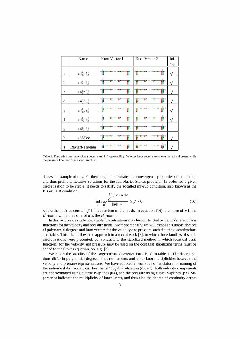
Table 1: Discretization names, knot vectors and inf-sup-stability. Velocity knot vectors are shown in red and green, whilethe pressure knot vector is shown in blue.

shows an example of this. Furthermore, it deteriorates the convergence properties of the methodand thus prohibits iterative solutions for the full Navier-Stokes problem. In order for a givendiscretization to be stable, it needs to satisfy the socalled inf-sup condition, also known as theBB or LBB condition:

infp

supu

∫∫

Ω

p∇ · u dA

‖p‖ ‖u‖ ≥ β > 0, (16)

where the positive constantβ is independent of the mesh. In equation (16), the norm ofp is theL2-norm, while the norm ofu is theH1-norm.

In this section we study how stable discretizations may be constructed by using different basisfunctions for the velocity and pressure fields. More specifically, we will establish suitable choicesof polynomial degrees and knot vectors for the velocity and pressure such that the discretizationsare stable. This idea follows the approach in a recent work [7], in which three families of stablediscretizations were presented, but contrasts to the stabilized method in which identical basisfunctions for the velocity and pressure may be used on the cost that stabilizing terms must beadded to the Stokes equation, see e.g. [3].

We report the stability of the isogeometric discretizations listed in table 1. The discretiza-tions differ in polynomial degrees, knot refinements and inner knot multiplicities between thevelocity and pressure representations. We have adobted a heuristic nomenclature for naming ofthe individual discretizations. For theu42

0p310 discretization (d), e.g., both velocity components

are approximated using quartic B-splines (u4), and the pressure using cubic B-splines (p3). Su-perscript indicates the multiplicity of inner knots, and thus also the degree of continuity across

8

knots, since this is just the degree minus the multiplicity.Subscript indicates the number ofh-refinements by halfing all knot spans. For the strategies a-g,each of the velocity componenentsu1 andu2 are represented identically, which reduces the computational expenses since equalityof the basis functionsRu1

i = Ru2i implies equality of the matricesKi j1 = Ki j2, and in addition all

fields are represented identically in both parametric directions. This is not the case for the strate-gies h and i, which are modified versions of the Nedelec and Raviart-Thomas elements presentedin [7]. Compared to the original formulation in [7], the velocity fields have beenh-refined once.It should be stressed that with this enlargement of the velocity space, the exact fulfillment of thedivergence-free constraint for the Raviart-Thomas discretization is lost. Theu42

0p310 discretiza-

tion (d) was originally proposed in [3] and subsequently introduced in [7] as the Taylor-Hoodelement.

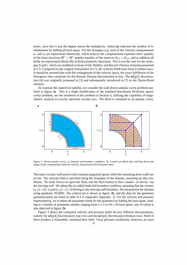
To examine the numerical stability, we consider the wall-driven annular cavity problem out-lined in figure 2a. This is a slight modification of the standard benchmarklid-driven squarecavity problem, see the treatment of the problem in Section 6, utilizing the capability of isoge-ometric analysis to exactly represent circular arcs. The fluid is contained in an annular cavity.

a b

0 1 2

0

1

2

x

y

u = 0

u=

0 u=

0

ut =1

ur=

0

f = 0

0 1 2

0

1

2

x

y

Figure 2: Driven annular cavity.a: Domain and boundary conditions.b: Control net (black dots and blue lines) andimage of the computational mesh for velocity and pressure (red and green lines).

The inner circular wall moves with constant tangential speed, while the remaining three walls areat rest. The velocity field is specified along the boundary of the domain, assuming no-slip con-ditions. No body forces act upon the fluid, and the fluid motionis thus caused—or driven—bythe moving wall. We adopt the so-calledleaky-lid boundary condition, meaning that the corners(x, y) = (0, 1) and (x, y) = (1, 0) belong to the moving wall boundary. We parametrise the domainusing quadratic NURBS. The control net is shown in figure 2b, and the data for the geometryparametrisation are listed in table A.2 in Appendix Appendix A. For the velocity and pressurerepresentation, weh-refine the parameter mesh for the geometry by halfing the knotspans, lead-ing to a familiy of parameter meshes ranging from 2× 2 to 64× 64 knot spans, one of which isalso depicted in figure 2b.

Figure 3 shows the computed velocity and pressure fields for two different discretizations,namely theu41

0p410 discretization (top row) and theu41

1p410 discretization (bottom row). Both of

these produce a reasonable, rotational flow field. Clear pressure oscillations, however, are seen9

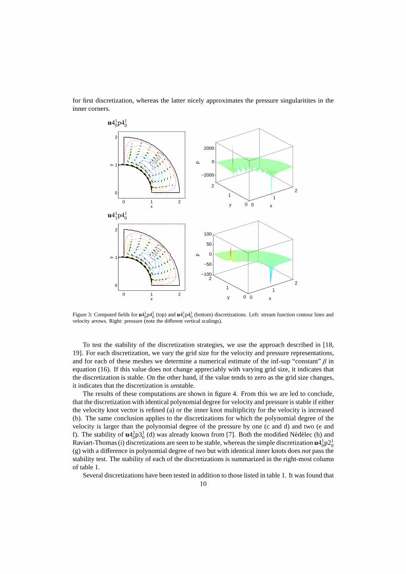
for first discretization, whereas the latter nicely approximates the pressure singularitites in theinner corners.

u410p41

0

0 1 2

0

1

2

x

y

−0.002−0.02−0.04−0.06−0.08−0.1−0.12

0

1

2

0

1

2

−2000

0

2000

xy

p

u411p41

0

0 1 2

0

1

2

x

y

−0.002−0.02−0.04−0.06−0.08−0.1−0.12

0

1

2

0

1

2−100

−50

0

50

100

xy

p

Figure 3: Computed fields foru410p41

0 (top) andu411p41

0 (bottom) discretizations. Left: stream function contour lines andvelocity arrows. Right: pressure (note the different vertical scalings).

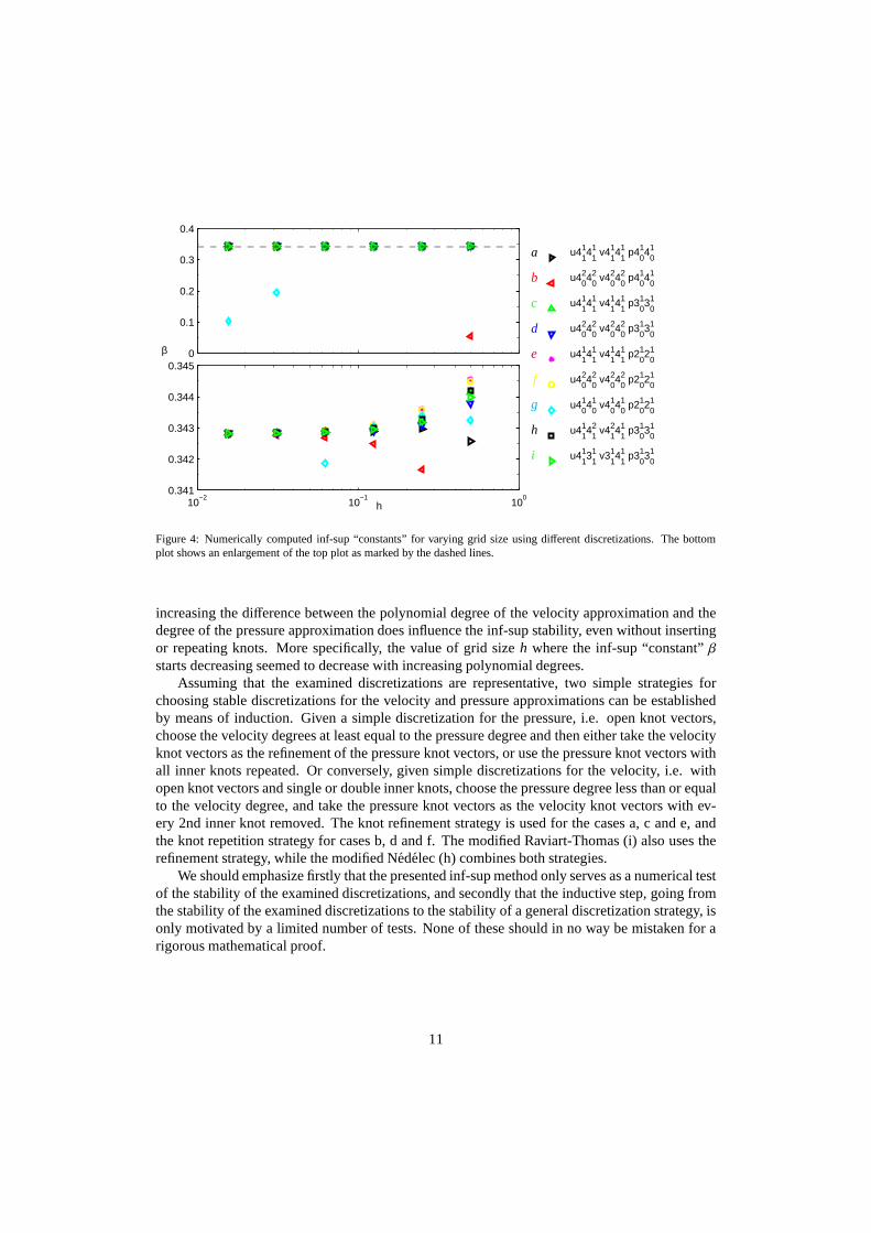
To test the stability of the discretization strategies, we use the approach described in [18,19]. For each discretization, we vary the grid size for the velocity and pressure representations,and for each of these meshes we determine a numerical estimate of the inf-sup “constant”β inequation (16). If this value does not change appreciably with varying grid size, it indicates thatthe discretization is stable. On the other hand, if the valuetends to zero as the grid size changes,it indicates that the discretization isunstable.

The results of these computations are shown in figure 4. From this we are led to conclude,that the discretization with identical polynomial degree for velocity and pressure is stable if eitherthe velocity knot vector is refined (a) or the inner knot multiplicity for the velocity is increased(b). The same conclusion applies to the discretizations forwhich the polynomial degree of thevelocity is larger than the polynomial degree of the pressure by one (c and d) and two (e andf). The stability ofu42

0p310 (d) was already known from [7]. Both the modified Nedelec (h) and

Raviart-Thomas (i) discretizations are seen to be stable, whereas the simple discretizationu410p21

0(g) with a difference in polynomial degree of two but with identical inner knots doesnot pass thestability test. The stability of each of the discretizations is summarized in the right-most columnof table 1.

Several discretizations have been tested in addition to those listed in table 1. It was found that10

0

0.1

0.2

0.3

0.4

10−2

10−1

100

0.341

0.342

0.343

0.344

0.345

β

h

u4114

11 v4

114

11 p4

014

01

u4024

02 v4

024

02 p4

014

01

u4114

11 v4

114

11 p3

013

01

u4024

02 v4

024

02 p3

013

01

u4114

11 v4

114

11 p2

012

01

u4024

02 v4

024

02 p2

012

01

u4014

01 v4

014

01 p2

012

01

u4114

12 v4

124

11 p3

013

01

u4113

11 v3

114

11 p3

013

01

a

b

c

d

e

f

g

h

i

Figure 4: Numerically computed inf-sup “constants” for varying grid size using different discretizations. The bottomplot shows an enlargement of the top plot as marked by the dashed lines.

increasing the difference between the polynomial degree of the velocity approximation and thedegree of the pressure approximation does influence the inf-sup stability, even without insertingor repeating knots. More specifically, the value of grid sizeh where the inf-sup “constant”βstarts decreasing seemed to decrease with increasing polynomial degrees.

Assuming that the examined discretizations are representative, two simple strategies forchoosing stable discretizations for the velocity and pressure approximations can be establishedby means of induction. Given a simple discretization for thepressure, i.e. open knot vectors,choose the velocity degrees at least equal to the pressure degree and then either take the velocityknot vectors as the refinement of the pressure knot vectors, or use the pressure knot vectors withall inner knots repeated. Or conversely, given simple discretizations for the velocity, i.e. withopen knot vectors and single or double inner knots, choose the pressure degree less than or equalto the velocity degree, and take the pressure knot vectors asthe velocity knot vectors with ev-ery 2nd inner knot removed. The knot refinement strategy is used for the cases a, c and e, andthe knot repetition strategy for cases b, d and f. The modifiedRaviart-Thomas (i) also uses therefinement strategy, while the modified Nedelec (h) combines both strategies.

We should emphasize firstly that the presented inf-sup method only serves as a numerical testof the stability of the examined discretizations, and secondly that the inductive step, going fromthe stability of the examined discretizations to the stability of a general discretization strategy, isonly motivated by a limited number of tests. None of these should in no way be mistaken for arigorous mathematical proof.

11

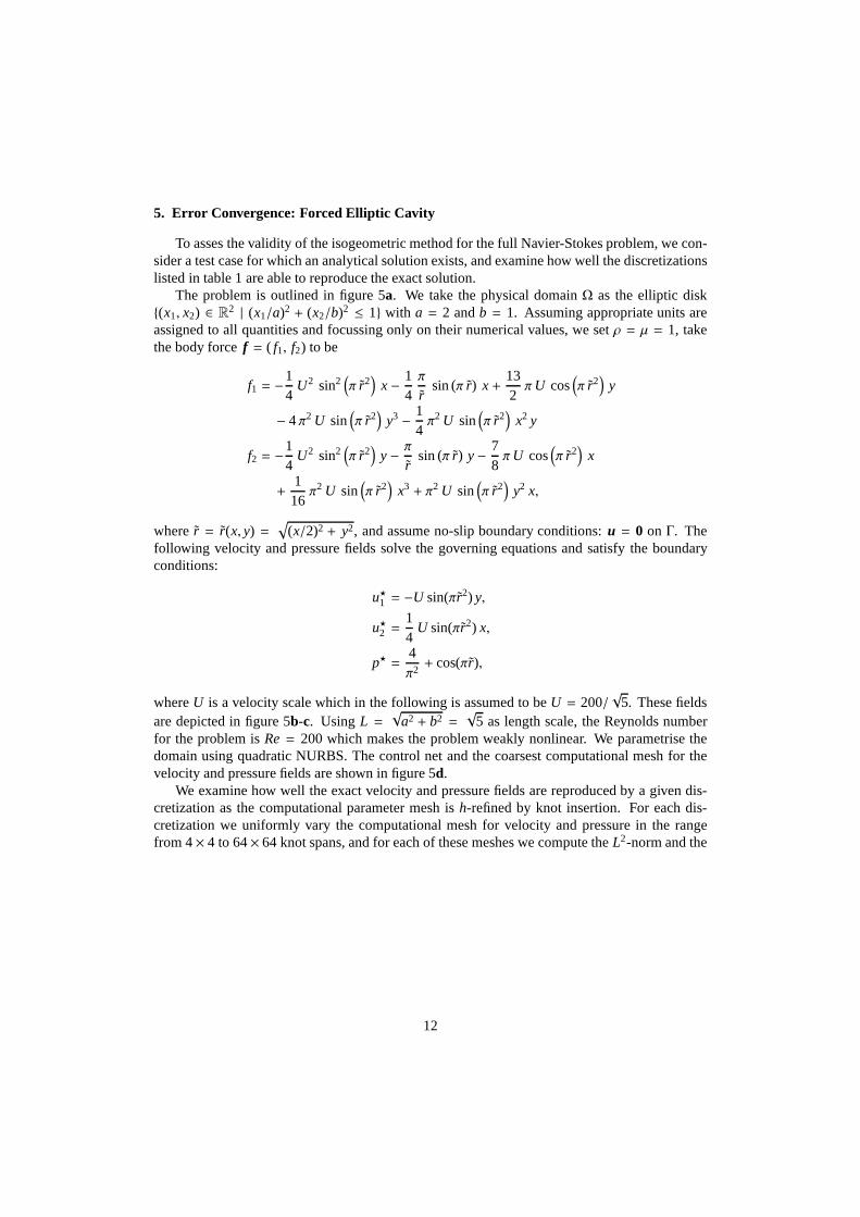
5. Error Convergence: Forced Elliptic Cavity

To asses the validity of the isogeometric method for the fullNavier-Stokes problem, we con-sider a test case for which an analytical solution exists, and examine how well the discretizationslisted in table 1 are able to reproduce the exact solution.

The problem is outlined in figure 5a. We take the physical domainΩ as the elliptic disk(x1, x2) ∈ R

2 | (x1/a)2 + (x2/b)2 ≤ 1 with a = 2 andb = 1. Assuming appropriate units areassigned to all quantities and focussing only on their numerical values, we setρ = µ = 1, takethe body forcef = ( f1, f2) to be

f1 = −14

U2 sin2(π r2)

x − 14π

rsin(π r) x +

132πU cos

(π r2)

y

− 4π2 U sin(π r2)

y3 − 14π2 U sin

(π r2)

x2 y

f2 = −14

U2 sin2(π r2)

y − πr

sin(π r) y − 78πU cos

(π r2)

x

+116π2 U sin

(π r2)

x3 + π2 U sin(π r2)

y2 x,

wherer = r(x, y) =√

(x/2)2 + y2, and assume no-slip boundary conditions:u = 0 on Γ. Thefollowing velocity and pressure fields solve the governing equations and satisfy the boundaryconditions:

u⋆1 = −U sin(πr2) y,

u⋆2 =14

U sin(πr2) x,

p⋆ =4π2+ cos(πr),

whereU is a velocity scale which in the following is assumed to beU = 200/√

5. These fieldsare depicted in figure 5b-c. Using L =

√a2 + b2 =

√5 as length scale, the Reynolds number

for the problem isRe = 200 which makes the problem weakly nonlinear. We parametrise thedomain using quadratic NURBS. The control net and the coarsest computational mesh for thevelocity and pressure fields are shown in figure 5d.

We examine how well the exact velocity and pressure fields arereproduced by a given dis-cretization as the computational parameter mesh ish-refined by knot insertion. For each dis-cretization we uniformly vary the computational mesh for velocity and pressure in the rangefrom 4× 4 to 64× 64 knot spans, and for each of these meshes we compute theL2-norm and the

12

a b

−3 −2 −1 0 1 2 3−1.5

−1

−0.5

0

0.5

1

1.5

x

y

u = 0

f = ( f1, f2)

−3 −2 −1 0 1 2 3−1.5

−1

−0.5

0

0.5

1

1.5

x

y

c d

−3 −2 −1 0 1 2 3−1.5

−1

−0.5

0

0.5

1

1.5

x

y

−3 −2 −1 0 1 2 3−1.5

−1

−0.5

0

0.5

1

1.5

x

y

Figure 5: Forced elliptic cavity.a: Domain and boundary conditions.b: Analytical stream function contour lines andvelocity arrows.c: Analytical pressure contour lines.d: Control net (black dots and blue lines) and image of the coarsestcomputational mesh for velocity and pressure (red and greenlines).

H1-seminorm of the velocity residual and the pressure residual as measures of the error:

ǫ2u =

∫∫

Ω

‖u(x1, x2) − u⋆(x1, x2)‖2dx1dx2,

ǫ2p =

∫∫

Ω

|p(x1, x2) − p⋆(x1, x2)|2dx1dx2,

ǫ2∇u =

∫∫

Ω

2∑

k=1

‖∇uk(x1, x2) − ∇u⋆k (x1, x2)‖2dx1dx2,

ǫ2∇p =

∫∫

Ω

‖∇p(x1, x2) − ∇p⋆(x1, x2)‖2dx1dx2.

The results are shown in figure 6. The figure depicts the velocity error (top) and pressure error(bottom) as function of the total number of variables of the analysis, using both theL2-norm (left)and theH1-seminorm (right). We note that the discretizations a-f which pairwise have identicalpolynomial degrees, the knot refinement strategies (a, c, e)have a significantly lower velocityerror than the knot repetion strategies (b, d, f). In addition, the difference between the twostrategies grows as the number of degrees of fredoom increases, as is most evident for theH1-seminorm. The difference in pressure error between the two strategies varies more, but the errorof the knot refinement strategy is never larger than the errorof the corresponding knot repetionstrategy. This make the knot refinement strategy favorable in a per-degree-of-freedomsense. Theknot refinement strategy, unlike the knot repetition strategy, conserves the degree of continuityfor the velocity field. This therefore confirms the high importance of continuity alluded to in

13

10−5

100

εu

102

103

104

105

10−5

100

εp

Nvar

10−6

10−4

10−2

100

102

ε∇ u

102

103

104

10510

−6

10−4

10−2

100

102

ε∇ p

Nvar

u4114

11 v4

114

11 p4

014

01

u4024

02 v4

024

02 p4

014

01

u4114

11 v4

114

11 p3

013

01

u4024

02 v4

024

02 p3

013

01

u4114

11 v4

114

11 p2

012

01

u4024

02 v4

024

02 p2

012

01

u4014

01 v4

014

01 p2

012

01

u4114

12 v4

124

11 p3

013

01

u4113

11 v3

114

11 p3

013

01

a

b

c

d

e

f

g

h

i

Figure 6: Convergence of error:L2-norm (left) andH1-seminorm (right) of velocity residual (top) and pressure residual(bottom) as function of the total number of variables of the analysis using different discretizations.

[4]. However, although the increase in number of degrees of freedom for a given refinementis nearly identical for the two strategies, the knot refinement strategy is computationally moreexpensive than the knot repetition strategy, since it doubles the number of knot spans and thusquadruples the number of function evaluations needed for the Gaussian quadrature, unless moreefficient quadrature rules are employed [17]. It is also worth noting that although the pressureerror of the unstable discretizationu41

0p210 (g) flattens out quit quickly as the number of degrees of

freedom increases, the velocity error falls off impressively. Lastly, the modified Raviart-Thomasdiscretization (h) seem to perform somewhat better than themodified Nedelec discretization (i)for both the velocity and the pressure.

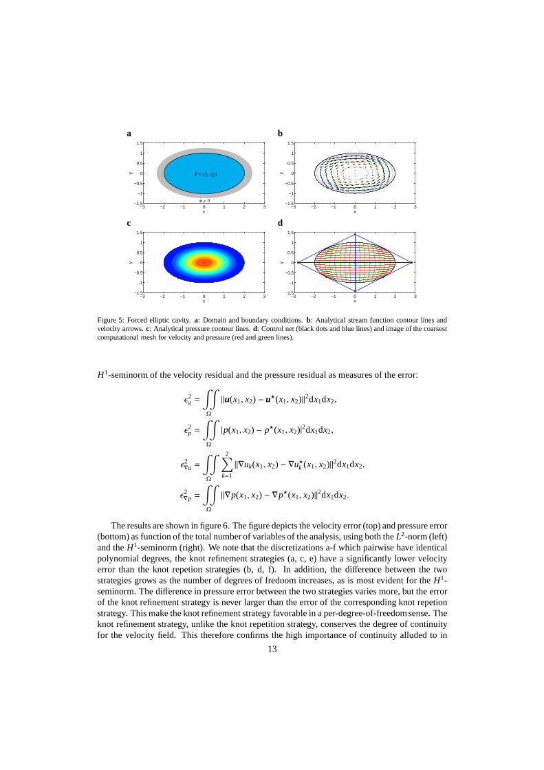
We have in general good experiences with the Taylor-Hood discretizationu420p31

0 (d), since itdiscretizes both velocity components identically, and theknot spans for the velocity and pressurefields are also the same. We therefore base the following examination of the influence of theformulations of the Navier-Stokes equation on this discretization. We solve the problem outlinedabove using both the convective formulation as above and theskew-symmetric formulation, andwe do this for two different values of the Reynolds number, namely 200 and 2,000, using 400;800; 1,000; 1,500 as intermediate values to ensure convergence. Figure 7 compares the con-vergence of errors for the two formulations. For the low Reynolds number, both the velocityand the pressure errors of the two formulations are practically identical. For the higher Reynoldsnumber, some differences are seen for the pressure error, while the velocity errors remain similar.It should also be mentioned that in our experience, more non-linear solver iterations are neededfor the skew-symmetric formulation to converge compared tothe convective formulation.

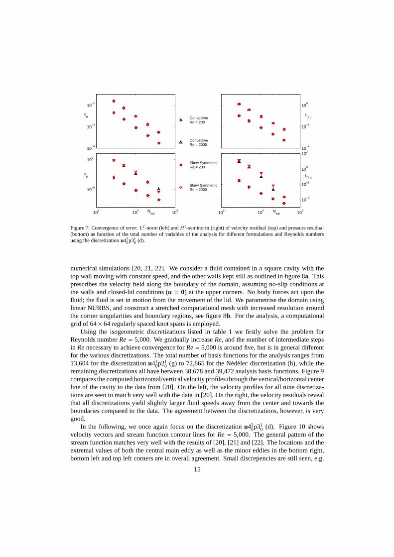
6. Benchmark: Lid-Driven Square Cavity

As a final validation of the isogeometric method, we compare our results for a standardbenchmark flow problem, namely the lid-driven square cavity[12, 3], against results from other

14

10−6

10−4

10−2

εu

103

104

105

10−5

100

εp

Nvar

10−4

10−2

100

ε∇ u

103

104

105

10−4

10−2

100

102

ε∇ p

Nvar

ConvectiveRe = 200

ConvectiveRe = 2000

Skew SymmetricRe = 200

Skew SymmetricRe = 2000

Figure 7: Convergence of error:L2-norm (left) andH1-seminorm (right) of velocity residual (top) and pressure residual(bottom) as function of the total number of variables of the analysis for different formulations and Reynolds numbersusing the discretizationu42

0p310 (d).

numerical simulations [20, 21, 22]. We consider a fluid contained in a square cavity with thetop wall moving with constant speed, and the other walls keptstill as outlined in figure 8a. Thisprescribes the velocity field along the boundary of the domain, assuming no-slip conditions atthe walls and closed-lid conditions (u = 0) at the upper corners. No body forces act upon thefluid; the fluid is set in motion from the movement of the lid. Weparametrise the domain usinglinear NURBS, and construct a stretched computational meshwith increased resolution aroundthe corner singularities and boundary regions, see figure 8b. For the analysis, a computationalgrid of 64× 64 regularly spaced knot spans is employed.

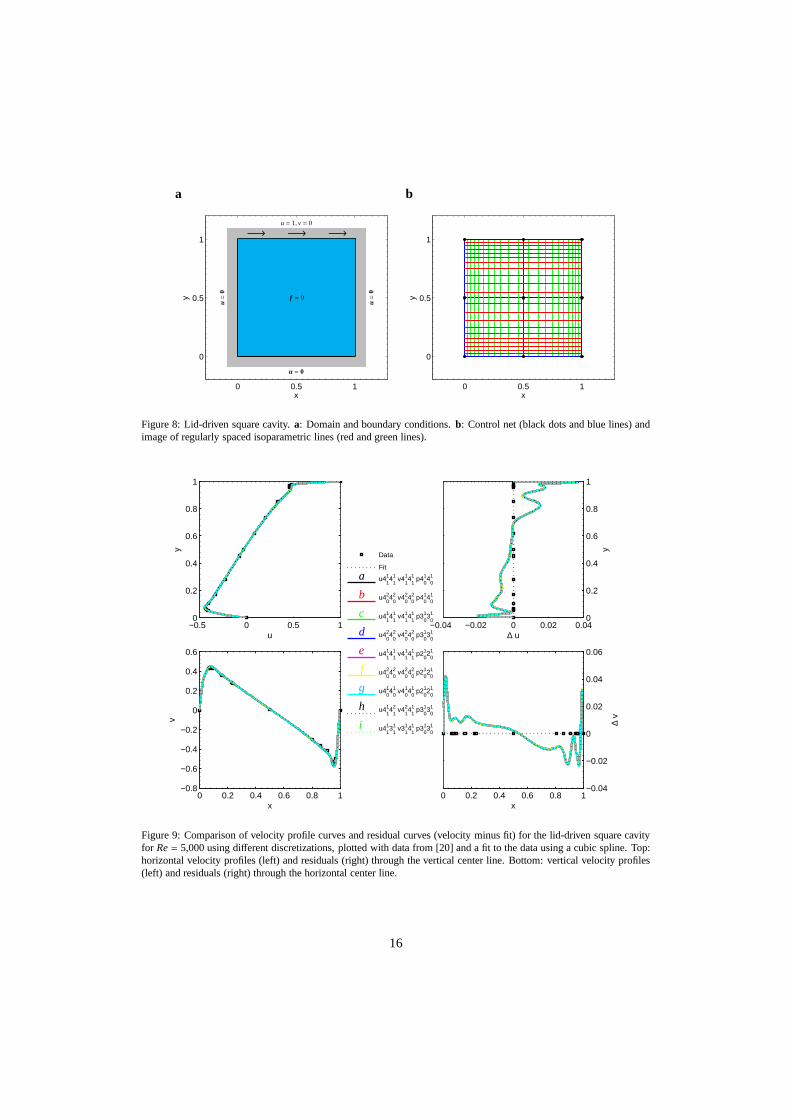
Using the isogeometric discretizations listed in table 1 wefirstly solve the problem forReynolds numberRe = 5,000. We gradually increaseRe, and the number of intermediate stepsin Re necessary to achieve convergence forRe = 5,000 is around five, but is in general differentfor the various discretizations. The total number of basis functions for the analysis ranges from13,604 for the discretizationu41

0p210 (g) to 72,865 for the Nedelec discretization (h), while the

remaining discretizations all have between 38,678 and 39,472 analysis basis functions. Figure 9compares the computed horizontal/vertical velocity profiles through the vertical/horizontal centerline of the cavity to the data from [20]. On the left, the velocity profiles for all nine discretiza-tions are seen to match very well with the data in [20]. On the right, the velocity residuals revealthat all discretizations yield slightly larger fluid speedsaway from the center and towards theboundaries compared to the data. The agreement between the discretizations, however, is verygood.

In the following, we once again focus on the discretizationu420p31

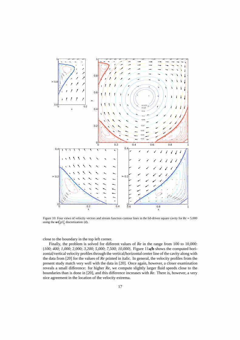
0 (d). Figure 10 showsvelocity vectors and stream function contour lines forRe = 5,000. The general pattern of thestream function matches very well with the results of [20], [21] and [22]. The locations and theextremal values of both the central main eddy as well as the minor eddies in the bottom right,bottom left and top left corners are in overall agreement. Small discrepencies are still seen, e.g.

15

a b

0 0.5 1

0

0.5

1

x

y

u=

0

u=

0u = 0

u = 1, v = 0

f = 0

−→ −→ −→

0 0.5 1

0

0.5

1

x

y

Figure 8: Lid-driven square cavity.a: Domain and boundary conditions.b: Control net (black dots and blue lines) andimage of regularly spaced isoparametric lines (red and green lines).

0 0.2 0.4 0.6 0.8 1−0.8

−0.6

−0.4

−0.2

0

0.2

0.4

0.6

x

v

Data

Fit

u4114

11 v4

114

11 p4

014

01

u4024

02 v4

024

02 p4

014

01

u4114

11 v4

114

11 p3

013

01

u4024

02 v4

024

02 p3

013

01

u4114

11 v4

114

11 p2

012

01

u4024

02 v4

024

02 p2

012

01

u4014

01 v4

014

01 p2

012

01

u4114

12 v4

124

11 p3

013

01

u4113

11 v3

114

11 p3

013

01

−0.5 0 0.5 10

0.2

0.4

0.6

0.8

1

u

y

0 0.2 0.4 0.6 0.8 1−0.04

−0.02

0

0.02

0.04

0.06

x

∆ v

−0.04 −0.02 0 0.02 0.040

0.2

0.4

0.6

0.8

1

∆ u

y

a

b

c

d

e

f

g

h

i

Figure 9: Comparison of velocity profile curves and residualcurves (velocity minus fit) for the lid-driven square cavityfor Re = 5,000 using different discretizations, plotted with data from [20] and a fit to the data using a cubic spline. Top:horizontal velocity profiles (left) and residuals (right) through the vertical center line. Bottom: vertical velocityprofiles(left) and residuals (right) through the horizontal centerline.

16

0 0.2 0.4 0.6 0.8 10

0.2

0.4

0.6

0.8

1

x

y

−0.1175

−0.115

−0.11

−0.1

−0.09

−0.07

−0.05

−0.03

−0.01

0 0.20.6

0.8

1

x

y

0.0010.0005

0.00025

0.00015e−

051e−05

0 0.2 0.40

0.2

0.4

x

y

0.001

0.00050.000250.0001

5e−051e−051e−06

0.6 0.8 10

0.2

0.4

x

y

0.00

3

0.0015

0.001

0.0005

0.00025

0.00015e−05

1e−05

Figure 10: Four views of velocity vectors and stream function contour lines in the lid-driven square cavity forRe = 5,000using theu42

0p310 discretization (d).

close to the boundary in the top left corner.Finally, the problem is solved for different values ofRe in the range from 100 to 10,000:

100; 400; 1,000; 2,000;3,200; 5,000; 7,500; 10,000. Figure 11a/b shows the computed hori-zontal/vertical velocity profiles through the vertical/horizontal center line of the cavity along withthe data from [20] for the values ofRe printed in italic. In general, the velocity profiles from thepresent study match very well with the data in [20]. Once again, however, a closer examinationreveals a small difference: for higherRe, we compute slightly larger fluid speeds close to theboundaries than is done in [20], and this difference increases withRe. There is, however, a verynice agreement in the location of the velocity extrema.

17

0 0.2 0.4 0.6 0.8 1

0

0

0

0

0

0

0

x

v

Re

= 1

00

Re

= 4

00

Re

= 1

000

Re

= 3

200

Re

= 5

000

Re

= 7

500

Re

= 10

000

0 0 0 0 0 0 0 10

0.2

0.4

0.6

0.8

1

u

y

Re = 100Re = 400

Re = 1000Re = 3200

Re = 5000Re = 7500

Re = 10000

−0.1 −0.05 0 0.05 0.10

0.2

0.4

0.6

0.8

1

∆ u

y

0 0.2 0.4 0.6 0.8 1−0.1

−0.05

0

0.05

0.1

x

∆ v

a

b

c

d

Figure 11: Velocity profile curves for the lid-driven squarecavity for seven values ofRe (solid lines) using theu420p31

0discretization (d) plotted along with data from [20] (points). a: vertical velocity profile through the horizontal center line.b: horizontal velocity profile through the vertical center line.c: vertical velocity residual.d: horizontal velocity residual.The profile curves have been translated to avoid clustering of data. We speculate that three obvious outliers, marked withrings, stem from misprints in the tabulated data in [20]. Cubic splines have been fitted to the remaining data.

18

Regarding the differences in flow speeds close to the boundaries, several points deserve men-tioning. Firstly, the results depend critically on the choice of boundary conditions specified forthe upper corners. We emphasize that closed-lid conditionsare assumed in the present study.Secondly, the results depend slightly on the formulation ofthe Navier-Stokes equation (1a) forRe & 5,000, depending on whether the convective or the skew-symmetric formulation is used.This is shown in figure 12, where the computed velocity profiles using each of the two differentformulations are compared forRe = 10,000. The convective and the skew-symmetric formula-

0 0.2 0.4 0.6 0.8 1−0.8

−0.6

−0.4

−0.2

0

0.2

0.4

0.6

x

v

Data

Fit

Convective

Skew−Symmetric

−0.5 0 0.5 10

0.2

0.4

0.6

0.8

1

u

y

0 0.2 0.4 0.6 0.8 1−0.05

0

0.05

0.1

0.15

x

∆ v

−0.04 −0.02 0 0.02 0.040

0.2

0.4

0.6

0.8

1

∆ u

y

Figure 12: Comparison of velocity profile curves and residual curves (velocity minus fit) for the lid-driven square cavityfor Re = 10,000 with different formulations of the inertial term using theu42

0p310 discretization (d), plotted with data

from [20] and a fit to the data using a cubic spline. Top: horizontal velocity profiles (left) and residuals (right) throughthe vertical center line. Bottom: vertical velocity profiles (left) and residuals (right) through the horizontal center line.

tions are found to nearly match each other in the interior, whereas some differences are observedclose to the boundaries, in particular at the moving lid. We emphasize that the present studyis based on the simpler convective formulation of the Navier-Stokes equation. Thirdly, the datain [20] are relatively sparse at the boundaries where the variation in velocity is high. Finally, itshould be stressed that the data in [20] stem from another numerical study, and an exact corre-spondence between that and the present study should not be expected.

7. Conclusions

This paper has examined various discretizations in isogeometric analysis of 2-dimensional,steady state, incompressible Navier-Stokes equation subjected to Dirichlet boundary conditions.Firstly, a detailed description of the implementation has been given. Secondly, numerical inf-supstability tests have been presented that confirm the existence of many stable discretizations of

19

Wall-Driven Annular Cavity

Degree q = r = 2Knots Ξ = Φ = 0,0, 0,1, 1,1Point 1 2 3 4 5 6 7 8 9x1 0 1 1 0 3/2 3/2 0 2 2x2 1 1 0 3/2 3/2 0 2 2 0w 1 1/

√2 1 1 1/

√2 1 1 1/

√2 1

Forced Elliptic Cavity

Degree q = r = 2Knots Ξ = Φ = 0,0, 0,1, 1,1Point 1 2 3 4 5 6 7 8 9x1 −2/

√2 0 2/

√2 −4/

√2 0 4/

√2 −2/

√2 0 2/

√2

x2 −1/√

2 −2/√

2 −1/√

2 0 0 0 1/√

2 2/√

2 1/√

2w 1 1/

√2 1 1 1/

√2 1 1 1/

√2 1

Lid-Driven Square Cavity

Degree q = r = 1Knots Ξ = Φ = 0,0, 1/2,1, 1Point 1 2 3 4 5 6 7 8 9x1 0 1/2 1 0 1/2 1 0 1/2 1x2 0 0 0 1/2 1/2 1/2 1 1 1w 1 1/2 1 1/2 1/4 1/2 1 1/2 1

Table A.2: Polynomial degrees, knot vectors, control points and weights for the geometry of the analysed problems.

the velocity and pressure spaces. In particular it was foundthat stability may be achieved bymeans of knot refinement of the velocity space. Thirdly, error convergence studies compared theperformance of the various discretizations and indicated optimal convergence, in a per-degree-of-freedom sense, of the discretization with identical polynomial degrees of the velocity andpressure spaces but with the velocity space enriched by knotrefinement. Finally, the method hasbeen applied to the lid-driven square cavity for benchmarking purposes, showing that the stablediscretizations produce consistent results that match well with existing data and thus confirm therobustness of the method.

Appendix A. Data for Geometry Parametrisations

Table A.2 lists the polynomial degrees, knot vectors and control points for the geometry ofthe analysed problems.

References

[1] T. Hughes, J. Cottrell, Y. Bazilevs, Isogeometric analysis: CAD, finite elements, NURBS, exact geometry andmesh refinement, Comput. Methods Appl. Mech. Engrg. 194 (2005) 4135–4195.

[2] J. Cottrell, T. Hughes, Y. Bazilevs, Isogeometric Analysis: Toward Integration of CAD and FEA, John Wiley andSons, 2009.

20

[3] Y. Bazilevs, L. D. Veiga, J. Cottrell, T. Hughes, G. Sangalli, Isogeometric analysis: Approximation, stability anderror estimates forh-refined meshes, Mathematical Models and Methods in AppliedScience 16 (2006) 1031–1090.

[4] I. Akkerman, Y. Bazilevs, V. Calo, T. Hughes, S. Hulshoff, The role of continuity in residual-based variationalmultiscale modeling of turbulence., Comput. Mech. 41 (2010) 371–378.

[5] Y. Bazilevs, T. Hughes, NURBS-based isogeometric analysis for the computation of flows about rotating compo-nents, Comput. Mech. 43 (2008) 143–150.

[6] Y. Bazilevs, I. Akkerman, Large eddy simulation of turbulent taylor-couette flow using isogeometric analysis andthe residual-based variational multiscale method, Journal of Computational Physics 229 (2010) 3402–3414.

[7] A. Buffa, C. de Falco, G. Sangalli, Isogeometric Analysis: Stable elements for the 2D stokes equation, Int. J.Numer. Meth. Fluids (2011).

[8] A. Bressan, Isogeometric regular discretization for the Stokes problem, IMA Journal of Numerical Analysis2(2010).

[9] A. Bressan, Personal communication.[10] W. Layton, C. Manica, M. Neda, M. Olshanskii, L. Rebholz, On the accuracy of the rotation form in simulations

of the Navier-Stokes-equations, Journal of ComputationalPhysics 228 (2009) 3433–3447.[11] J. Reddy, D. Gartling, The finite element method in heat transfer and fluid dynamics, CRC Press, 2nd edition, 2001.[12] J. Donea, A. Huerta, Finite Element Methods for Flow Problems, John Wiley and Sons, 2003.[13] L. Piegl, W. Tiller, The NURBS Book, Springer, 1995.[14] Y. Bazilevs, T. Hughes, Weak imposition of Dirichlet boundary conditions in fluid mechanics, Computers & Fluids

36 (2007) 12–26.[15] Y. Bazilevs, C. Michler, V. Calo, T. Hughes, Weak Dirichlet boundary conditions for wall-bounded turbulent flows,

Comput. Methods Appl. Mech. Engrg. 196 (2007) 4853–4862.[16] W. Wall, M. Frenzel, C. Cyron, Isogeometric structuralshape optimization, Comput. Methods Appl. Mech. Engrg.

197 (2008) 2976–2988.[17] T. Hughes, A. Reali, G. Sangalli, Efficient quadrature for NURBS-based isogeometric analysis, Comput. Methods

Appl. Mech. Engrg. 199 (2010) 301–313.[18] D. Chapelle, K. Bathe, The inf-sup test, Computers & Structures 47 (1993) 537–545.[19] K. Bathe, The inf-sup condition and its evaluation for mixed finite element methods, Computers & Structures 79

(2001) 243–252.[20] U. Ghia, K. Ghia, C. Shin, High-Re Solution for Incompressible Flow Using the Navier-Stokes Equations and a

Multigrid Method, Journal of Computational Physics 48 (1982) 387–411.[21] E. Erturk, T. Corke, C. Gokcol, Numerical solutions of 2-d steady incompressible driven cavity flow at high

Reynolds numbers, Int. J. Numer. Meth. Fluids48 (2005) 747–774.[22] L. Lee, A class of high-resolution algorithms for incompressible flows, Computers & Fluids 39 (2010) 1022–1032.

21