Discussion Paper Series

A Theory of Infrastructure-led Development

By

Pierre-Richard Agénor

Centre for Growth and Business Cycle Research, Economic Studies, University of Manchester, Manchester, M13 9PL, UK

December 2006

Number 083

Download paper from:

http://www.ses.man.ac.uk/cgbcr/discussi.htm

A Theory

of Infrastructure-Led Development

Pierre-Richard Agénor∗

Final version: February, 5 2010

Abstract

This paper proposes a theory of long-run development based on

public infrastructure as the main engine of growth. The government,

in addition to investing in infrastructure, spends on health services,

which in turn raise labor productivity and lower the rate of time pref-

erence. Infrastructure affects the production of both commodities and

health services. As a result of network effects, the degree of efficiency

of infrastructure is nonlinearly related to the stock of public capital it-

self. This in turn may generate multiple equilibria. Provided that gov-

ernance is adequate enough to ensure a sufficient degree of efficiency

of public investment outlays, an increase in the share of spending on

infrastructure (financed by a cut in unproductive expenditure or for-

eign grants) may facilitate the shift from a low growth equilibrium,

characterized by low productivity and low savings, to a high growth

steady state.

JEL Classification Numbers: O41, H54, I28.

∗Hallsworth Professor of International Macroeconomics and Development Economics,University of Manchester, and Centre for Growth and Business Cycle Research. I am

grateful to Keith Blackburn, Peter Montiel, Kyriakos Neanidis, Devrim Yilmaz, partici-

pants at seminars at the Universities of Naples (Parthenope) and Clermont-Ferrand, and

two referees for helpful discussions and comments on a previous draft. I also thank Steven

Pierce for providing relevant historical references on the role of infrastructure (or, rather,

the lack thereof) in Sub-Saharan Africa. The views expressed here are my own.

1

Means of communication were not constructed in the colonial period... to

facilitate internal trade in African commodities. There were no roads connecting

different colonies and different parts of the same colony in a manner that made

sense with regard to Africa’s needs and development. All roads and railways

led down to the sea. They were built to extract gold or manganese or coffee

or cotton. They were built to make business possible for the timber companies,

trading companies and agricultural concession firms, and for white settlers.

Walter Rodney, How Europe Underdeveloped Africa (1973, Chapter 6).

1 Introduction

Lack of infrastructure continues to be a key obstacle to growth and devel-

opment in many low-income countries. In Sub-Saharan Africa in particular,

only 16 percent of roads are paved, and less than one in five Africans has

access to electricity. Transport costs are the highest in the world and act

as a significant constraint on trade expansion. Yoshino (2008) for instance

found that poor quality of public infrastructure–measured in terms of the

average numbers of days per year for which firms experience disruptions

in electricity–has an adverse effect on exports in sub-Saharan Africa. In

Rwanda, farmers receive only 20 percent of the price of their coffee as it is

loaded onto ships in Monbasa; the other 80 percent disappear into the costs

of poor roads (as well as red tape) between Rwanda and Kenya.

To alleviate these constraints to growth and poverty reduction, several

observers have advocated a large increase in public investment in infrastruc-

ture, in line with the “Big Push” view of Rosenstein Rodan (1943).1 A

common argument for doing so is that infrastructure services have a strong

1Actually, most of Rosenstein Rodan’s article is dedicated to the role of complemetar-

ities between industries, not to a large increase in public investment. However, in keeping

with tradition, we will credit the “Big Push” view to him.

2

growth-promoting effect through their impact on production costs, the pro-

ductivity of private inputs, and the rate of return on capital–particularly

when, to begin with, stocks of infrastructure assets are relatively low. More

recent research, however, has emphasized that infrastructure may also affect

growth indirectly through a variety of channels, most notably by affecting

health outcomes.2 Access to clean water and sanitation helps to improve

health and thereby productivity. By reducing the cost of boiling water, and

reducing the need to rely on smoky traditional fuels (such as wood, crop

residues, and charcoal) for cooking, access to electricity also helps to im-

prove hygiene and health–in the latter case by reducing indoor air pollution

and the incidence of respiratory illnesses.

Dwelling in part on this evidence, this paper presents a theory of de-

velopment based on public infrastructure as the main engine of growth. In

doing so, I deliberately leave aside two other powerful forces that have been

identified in the literature: human capital accumulation and endogenous

technological progress (see, for instance, Kosempel (2004)). In the model,

the growth rate depends on the interactions between infrastructure, health,

and savings. Infrastructure raises the economy’s ability to produce health

services; in turn, greater access to health services enhances workers’ produc-

tivity, and therefore output. Thus, the accumulation of human capital results

not from the acquisition of knowledge, but from better quality of effective

labor. Unlike endogenous growth models in the Uzawa-Lucas tradition, this

requires thinking of knowledge as embodied in workers, as opposed to books

and libraries. In addition, improvements in health raise incentives to save.

This effect occurs not through its direct impact on life expectancy–given

2See Agénor and Neanidis (2006) and Agénor (2009b) for a more detailed discussion

of these channels, and Wang (2003) and Wagstaff and Cleason (2004) for some empirical

evidence.

3

that the representative household in the model is infinitely-lived–but by re-

ducing the degree of impatience, or equivalently, preference for the present.

In turn, a lower time preference rate raises the marginal utility of future

consumption and stimulates savings, which promotes physical capital accu-

mulation and growth.

I also assume, crucially, that the degree of efficiency of public infrastruc-

ture is positively (and nonlinearly) related to the stock of public capital

itself. The threshold variable is the stock of capital per worker, as suggested

by Fernald (1999). The introduction of this external effect leads to multiple

equilibria. The realization of a specific steady-growth equilibrium depends

therefore on expectations of private agents and the initial position of the

economy–including the parameters characterizing public policy.

The existence of a nonlinear relationship between the efficiency of public

capital and its level can be motivated in two ways. The first is based on

the view that infrastructure investment is lumpy, that is, a certain quantity

of infrastructure assets must be accumulated before it begins to contribute

at all to the production activities of the private sector. However, lumpiness

can explain piecewise-linear threshold effects, but not necessarily nonconvex-

ities. The second is based on network effects. Economies of scale due to

network externalities are a widely recognized imperfection in infrastructure

services (see World Bank (1994)). An important characteristic of modern

infrastructure is indeed the fact that services are often supplied through a

networked delivery system designed to serve a multitude of users. This inter-

connectedness means that the benefits from investment at one point in the

network will generally depend on capacities at other points. Put differently,

inherent to the structure of a network is that many components are required

for the provision of a service; these components are thus complementary to

4

each other. Having electricity to produce commodities in rural areas but no

roads to carry them to urban markets limits the productivity effects of a

program designed to increase access to energy. In that sense, electricity and

roads are complementary components of the infrastructure network, and only

joint availability or operation will generate efficiency gains, that is, positive

externalities.

The network character of infrastructure capital may therefore induce a

strong nonlinearity in its productivity. Until the network is built, public

capital has a low (or even null) marginal productivity. Once the basic parts of

a network are established, and a critical mass has been reached, strong gains

are associated with small additional increases in infrastructure investment.

But beyond that, the productivity gains induced by additional investments

tend to slow down. Thus, in contrast to much of the literature on network

externalities, which is static in nature (as noted by Economides (1996)), the

perspective adopted here is explicitly dynamic.

This second interpretation carries substantial weight for understanding

the current plight of many poor countries. As noted earlier, inadequate

transport networks remain a key characteristic of Sub-Saharan Africa today.

Moreover, a number of observers have argued that the current state of affairs

is intimately linked to the history of the continent. Colonization and a focus

on resource extraction dramatically affected the use of space in the region,

shifting growth and urbanization from inland to coastal areas. Many African

capitals today are ports that were built at the end of railways designed to

carry flows of rawmaterials and labor from the inland. Historians like Cooper

(1993), as well as geographers and political scientists–particularly those in

the Marxist tradition, like Walter Rodney (1973), in his classic book How

Europe Underdeveloped Africa, as quoted above–have long pointed out that

5

transport networks inherited from that growth were located perpendicularly

to the seashores, and were not built to occupy space widely.3 As indicated

earlier, however, I go beyond a “pure” infrastructure (or physical capital)

view of development by accounting for the impact of infrastructure on the

production of health services and endogenizing the impact of health on labor

productivity and savings. The model illustrates therefore the crucial links

between public infrastructure accumulation and the joint evolution of private

physical capital, productivity, and incentives to save.

The remainder of the paper is organized as follows. Section 2 presents

the basic framework, which takes as given the degree of efficiency of public

capital. Section 3 derives the balanced growth path and discusses stability

conditions. Section 4 endogenizes the efficiency of public capital in infrastruc-

ture, by relating it to the stock of infrastructure itself measured in proportion

of the private capital stock. Section 5 explores the policy implications of the

results and compares them with those obtained in some recent studies. I ex-

amine, in particular, how a shift in government spending allocation toward

infrastructure, financed by either a cut in unproductive expenditure or an in-

crease in foreign aid, affects equilibrium dynamics. This exercise is therefore

consistent with the Big Push view referred to earlier. In addition, I consider

the case where the government implements a budget-neutral shift in outlays

toward health. The final section offers some concluding remarks.

3By and large, however, mainstream economists have not followed this lead. In their

analysis of the historical causes of African underdevelopment, Bertocchi and Canova (2002)

for instance barely mention this aspect of colonization.

6

2 The Basic Framework

The economy that I consider is closed and populated by a single, infinitely-

lived household-producer (or household, for short). It produces a single

traded commodity, which can be used for either consumption or investment.

With the resources provided by a tax on output, the government invests in

infrastructure and spends on commodities, which are used to produce (when

combined with public capital in infrastructure) health services. It also spends

on “unproductive” activities–that is, activities that have no direct effect on

the supply of infrastructure or health services. Both categories of services

are assumed to be nonrival and nonexcludable.

2.1 Production of Commodities

Commodities, in quantity , are produced with private capital, , public

capital in infrastructure capital, , and “effective” labor, defined as the

product of the quantity of labor and a productivity index. In turn, produc-

tivity depends solely on the available supply of health services, , with a

strict proportionality relationship.4 Because the growth rate of the popu-

lation is zero and population size is normalized to unity, effective labor is

simply .

Assuming a Cobb-Douglas technology yields5

= ()

1−− = (

)(

) (1)

4It could be assumed that productivity depends not only on access to health services but

also directly on infrastructure as well. Better roads, for instance, allow an easier commute

to work, thereby reducing stress associated with traffic jams. This effect of infrastructure

on productivity could also be subject to nonlinearities similar to those related to the

production of commodities, as discussed later.5In what folllows, time subscripts are omitted for simplicity. Also, ≡ is used

to denote the time derivative of any variable .

7

where ∈ (0 1) and 0 is an efficiency parameter which I take as

constant for the moment. Thus, production of commodities exhibits constant

returns to scale in all factors.6 For simplicity, the flow of services provided by

each capital stock is taken to be directly proportional to the available stock.

2.2 Production of Health Services

As discussed in the introduction, public infrastructure in this economy im-

proves health outcomes, by providing for instance greater access to drinking

water or by facilitating garbage disposal through sewage systems. Specifi-

cally, I assume that production of health services requires combining govern-

ment spending on health, , and public capital in infrastructure. Assuming

also a Cobb-Douglas technology yields

=

1− (2)

where ∈ (0 1). The provision of health services takes place therefore underconstant returns to scale in and . In line with the evidence for many

poor countries, only the government provides health services.

2.3 Household

The household maximizes the discounted present value of utility:

max

=

Z ∞

0

ln exp(−) (3)

6See Eicher and Turnovsky (1999) for a discussion of the relation between the existence

of a balanced growth path and the assumption of constant returns to scale in endogenous

growth models. Note that the aggregate function (1) does not imply diminishing returns

to scale at the level of the individual firm. Indeed, as discussed in detail in Agénor (2009a),

it can be derived by assuming constant returns to scale with respect to private factors at

the firm level, and an externality (or congestion effect) measured in terms of the ratio

of the public capital stock to the aggregate private capital stock. In that case, however,

public capital is nonexcludable but partially rival.

8

where is consumption and 0 the subjective discount rate. For sim-

plicity, I assume that the instantaneous utility function is logarithmic in

consumption only. A more general specification would be to assume, as in

Agénor (2008) for instance, that utility is non-separable in consumption and

health services, that is

() =()1−1

1− 1 6= 1 0

where is the intertemporal elasticity of intertemporal substitution and

measures the relative contribution of health to utility. However, as can be

inferred from the results in the papers cited above, this specification would

simply complicate derivations and would not add much to the discussion as

long as 1–the empirically relevant case for developing countries, as

documented in a variety of studies (see Agénor and Montiel (2008)). For the

purpose at hand–and given my focus on growth, rather than welfare–the

logarithmic specification is simpler and I shall retain it throughout.7

The rate of time preference is assumed to depend negatively on consump-

tion of health services, and positively on the stock of private capital:

= ( ) (4)

with 0, and 0.

This specification differs in significant ways from the formulation first

proposed by Uzawa (1968), who introduced the idea of a relation between

the rate of time preference and consumption.8 In the present case, it is health

7Note also that, as discussed by Cazzavillan (1996) and Chen (2006), if government

spending exerts positive externalities on household preferences (in the form of increasing

returns to public expenditure in utility), multiple equilibria and indeterminacy may also

emerge.8More specifically, Uzawa (1968, p. 489) assumed that the change in the rate of time

preference at time is a positive function of the level of utility at time . Subsequently, in

9

services, not consumption of goods or commodities, that affect the degree of

impatience. The essential motivation here is that healthier individuals are

less myopic and tend to value the future more. This can be viewed as a way

to capture, in a representative agent model with infinite horizon, the “life

expectancy” effect typically emphasized in OLG models with endogenous

lifetimes (or mortality rates), as in the original contributions of Blanchard

(1985), which builds on Yaari (1965) and Buiter (1988), or more recently in

Aísa and Pueyo (2006), where the flow of government expenditure is taken

to affect the instantaneous probability of death.9 This specification is also

consistent with the evidence that poor people tend to have a relatively high

rate of time preference, as documented for instance by Lawrance (1991), if

one takes a further step and assumes that consumption of health services is

positively related to income.10

Moreover, I also assume that the rate of time preference is increasing in

wealth–or equivalently, here, given that there are no other (private) stores

of value in this economy, the stock of private physical capital. As discussed

by Mohsin (2004) and Kam (2005) in a different context, this link avoids

some of the difficulties posed by Uzawa preferences.11 For tractability, I will

their taxonomy of intertemporal utility functions, Shi and Epstein (1993, p. 62) charac-

terized Uzawa preferences as consisting of a relation between the rate of time preference

and (current and past) consumption levels.9See also Blackburn and Cipriani (2002), Chakraborty (2004), Bunzel and Qiao (2005),

and Hashimoto and Tabata (2005). Ehrlich and Kim (2005) endogenized the mortality rate

by assuming instead that the survival probability of individuals depends on consumption.10See Frederick, Loewenstein, and O’Donoghue (2002) for a review of the microeconomic

evidence linking discount rates and health outcomes.11In a standard model of optimal saving, Uzawa preferences require increasing marginal

impatience for stability; see for instance Epstein and Hynes (1983), and Obstfeld (1990) for

an intuitive diagrammatic exposition. The plausibility of increasing marginal impatience

has been questioned by many; Blanchard and Fischer (1989, p. 75) went as far as to

recommend avoiding the Uzawa specification because “...with its assumption [that the

richer are more impatient than the poor, it] is not particularly attractive as a description

of preferences.”

10

assume that can be specified as a function of the ratio of over , so

that

= (

) (5)

with 0 0 and 00 0.

The household’s resource constraint takes the simple form

= (1− ) − (6)

where ∈ (0 1) is the tax rate on income. For simplicity, I assume thatprivate capital does not depreciate.

The household takes the rate of time preference, the tax rate, and the

efficiency parameter as given when choosing the optimal time profile of con-

sumption. Using (1) and (6), the current-value Hamiltonian for problem (3)

can be written as

= ln + [(1− ) − ]

where is the costate variable associated with constraint (6). From the first-

order condition = 0 and the costate condition = − + ,

optimality conditions for this problem take the familiar form

1 = (7)

= [(

)−

] (8)

where ≡ (1− ), with ≡ 1−− , together with the budget constraint

(6) and the transversality condition

lim→∞

exp(−) = 0 (9)

11

2.4 Government

The government invests in infrastructure capital, , spends on health, ,

and on unproductive activities, . It also collects a proportional tax on

output. If fiscal deficits are precluded, the government budget constraint is

given by

+ + = (10)

Spending components are all taken to be fixed fractions of tax revenues:

= = (11)

where ∈ (0 1). The fixity of spending shares is justified by the fact thatthe goal here is to provide a positive, rather than normative, theory of growth

and development.

Combining (10) and (11), the government budget constraint can be rewrit-

ten as

+ + = 1 (12)

The stock of public capital in infrastructure evolves over time according

to

= (13)

where ∈ (0 1) is an efficiency parameter that measures the extent to whichinvestment flows translate into actual accumulation of public capital. The

case 1 reflects the view that investment spending on infrastructure is

subject to inefficiencies, which tend to limit their positive impact on the

public capital stock. Arestoff and Hurlin (2005) and Hurlin (2006), for in-

stance, estimate the value of to vary between 0.4 and 0.6 for developing

countries. As it turns out, this parameter (which can broadly be thought of

as an indicator of the quality of public sector management, or governance)

12

plays an important role in discussing the role of public policies in escaping

from a low-growth trap.12 For simplicity, public capital is assumed not to

depreciate.

Combining (6), (10), and (13) yields the equilibrium condition of the

market for commodities:

= + ( + ) + + (14)

3 Constant Efficiency

I first study the properties of the model with a constant efficiency parameter,

. In the present setting, a competitive equilibrium can be defined as follows:

Definition 1. A competitive equilibrium is a set of infinite sequences for

the allocations ∞=0, such that ∞=0 satisfy equations (7),(8), and (9), the path ∞=0 satisfies equations (2), (6), and (14),for given values of the tax rate, , the spending shares, , , and , and

the efficiency parameter, .

From equation (7),

= − (15)

whereas, from (11) and (13),

= (

) = −1 (

) (16)

where = . From (1), (2), and (11),

= ()(

1−

) = + ()

(1−)(

)(1−)

12Total unproductive spending includes not only but also the “efficiency loss” in

productive spending, (1−) . An interesting avenue to explore would be to endogenize ,

by linking it to the degree of corruption or political incentives (see, for instance, Robinson

and Torvik (2005)). However, this is well beyond the scope of this paper.

13

This expression can be rewritten as

= ()(1−)ΩΩ(+)Ω (17)

where Ω ≡ 1− (1− ) 0, so that Ω 1.

Combining this result with (16) yields

= 1Ω

(1−)ΩΩ−Ω (18)

Substituting (1) and (17) in the household budget constraint (6) yields

= (1− )()(1−)ΩΩ(+)Ω − (19)

where = .

Using (2), the health-private capital ratio, denoted , is given by

= (

)(

) = (

)1− = (

)1−

that is, using (11) and (17),

= ()1−[()

(1−)ΩΩ(+)Ω ]1−

so that

= ()(1−)Ω(1−)ΩΦΩ (20)

where Φ ≡ + (1− ) 0.

Substituting this result in (5) yields

= ( ; ) (21)

with ≡ 0ΦΩ 0 and ≡ 0(1− )Ω 0.

Substituting (8) in (15) yields = ( ) − , that is, using (17)

and (21),

= ()

(1−)ΩΩ(+)Ω − ( ; ) (22)

14

Equations (18), (19), and (22) can be further condensed into a first-order

nonlinear differential equation system in = and = :

=

(+)Ω

− ( ; ) + (23)

=

(1−)ΩΩn

1Ω−Ω − (1− ) (1−)Ω(+)Ω

o+ (24)

where

≡ −(1− )(+ )()(1−)ΩΩ 0 (25)

These two equations, together with an initial condition on at = 0, and

the transversality condition (9), characterize the dynamics of the economy.

The balanced-growth path (BGP) can therefore be defined as follows:

Definition 2. The BGP is a set of sequences ∞=0, constant spend-ing shares, tax rate, and efficiency parameter, satisfying Definition 1, such

that for an initial condition = 0 , equations (23) and (24) and the

transversality condition (9) are satisfied, the government budget constraint

(12) holds, and consumption, the stocks of private and public capital, all

grow at the same constant rate .

By implication, is also the rate of growth of output of commodities and

supply of health services. Using (7), the transversality condition (9) can be

rewritten as

lim→∞

−1 exp(−) = 0 (26)

which is also satisfied, because is constant along the BGP.

Based on the results in the Appendix, the following proposition can be

established:

Proposition 1. With a constant degree of efficiency of public infrastruc-

ture, the BGP is unique and locally determinate. A high degree of sensitivity

of the rate of time preference with respect to the health-private capital ratio

enhances stability.

15

From (18) and (22), the steady-state growth rate is given by the equiv-

alent forms

= 1Ω

(1−)ΩΩ−Ω (27)

= ()(1−)ΩΩ(+)Ω − ( ; ) (28)

where denotes the stationary value of .13

Adjustment toward the long-run equilibrium is illustrated in Figure 1,

using linearized versions of (23) and (24). Line corresponds to combina-

tions of ( ) for which = 0, whereas line corresponds to combinations

of ( ) for which = 0. Both lines are upward-sloping and saddlepath sta-

bility requires to cut from below. The saddlepath, , also has a

positive slope. The long-run equilibrium obtains at point .

To briefly illustrate the functioning of the model–and with an eye to

the Big Push policy recommendation discussed later on–consider an unex-

pected, budget-neutral increase in the share of spending on infrastructure, ,

offset by a reduction in unproductive expenditure (that is, = −).14Based on the results in the Appendix, as well as equations (27) and (28), the

following proposition can be established:

Proposition 2. An unexpected, permanent increase in the share of

investment in infrastructure, financed by a cut in unproductive expenditure

( = −), raises the steady-state growth rate as well as the steady-statevalues of the consumption-private capital ratio and the public-private capital

ratio.

13Equation (28) implies that for the steady state to be characterized by positive growth,

the discount rate cannot be too sensitive to the health-capital ratio.14See Agénor (2008) for an analysis of budget-neutral shifts in the spending shares

and . Growth- and welfare-maximizing spending allocations are also discussed in those

papers. Note that here, increases in productive spending shares would not involve a trade-

off per se, if they are offset by cuts in unproductive spending. I will return to this issue

later.

16

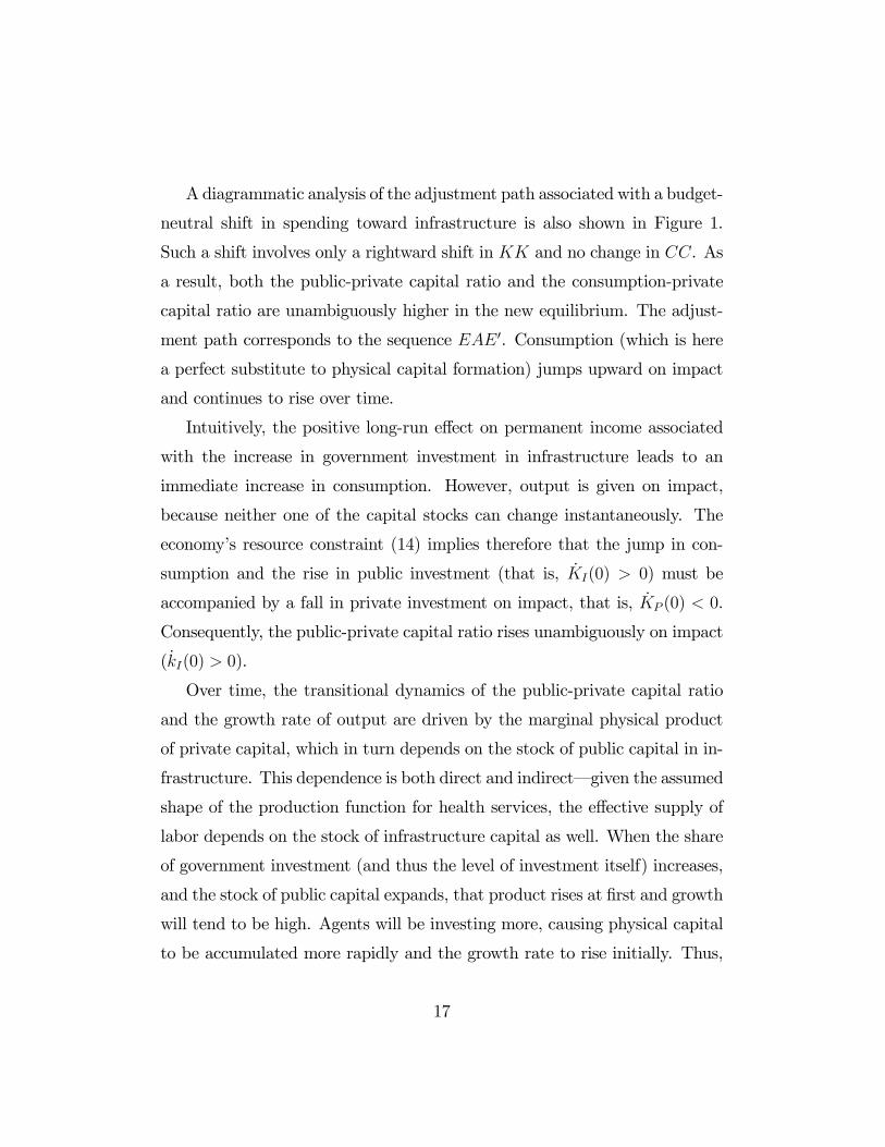
Adiagrammatic analysis of the adjustment path associated with a budget-

neutral shift in spending toward infrastructure is also shown in Figure 1.

Such a shift involves only a rightward shift in and no change in . As

a result, both the public-private capital ratio and the consumption-private

capital ratio are unambiguously higher in the new equilibrium. The adjust-

ment path corresponds to the sequence 0. Consumption (which is here

a perfect substitute to physical capital formation) jumps upward on impact

and continues to rise over time.

Intuitively, the positive long-run effect on permanent income associated

with the increase in government investment in infrastructure leads to an

immediate increase in consumption. However, output is given on impact,

because neither one of the capital stocks can change instantaneously. The

economy’s resource constraint (14) implies therefore that the jump in con-

sumption and the rise in public investment (that is, (0) 0) must be

accompanied by a fall in private investment on impact, that is, (0) 0.

Consequently, the public-private capital ratio rises unambiguously on impact

((0) 0).

Over time, the transitional dynamics of the public-private capital ratio

and the growth rate of output are driven by the marginal physical product

of private capital, which in turn depends on the stock of public capital in in-

frastructure. This dependence is both direct and indirect–given the assumed

shape of the production function for health services, the effective supply of

labor depends on the stock of infrastructure capital as well. When the share

of government investment (and thus the level of investment itself) increases,

and the stock of public capital expands, that product rises at first and growth

will tend to be high. Agents will be investing more, causing physical capital

to be accumulated more rapidly and the growth rate to rise initially. Thus,

17

the rate of private capital accumulation follows a nonmonotonic process: af-

ter falling at first (to accommodate the initial increase in consumption and

public investment, as noted earlier), it begins to rise, to reflect a greater rate

of return on physical assets.

But because the marginal product of private capital is negatively related

to the stock of private capital itself (given diminishing marginal returns to

all inputs), private investment will tend to fall over time as more of that type

of capital is accumulated. The transition to the steady-state growth rate will

be therefore characterized by a relatively high growth rate of private capital

and output initially, followed by a slowdown in both variables that may

vary in speed– depending on how quickly decreasing returns settle in. The

increase in private capital falls nevertheless short of the rate of accumulation

of public infrastructure assets, implying that the public-private capital ratio

rises continuously over time. In turn, the increase in that ratio tends to raise

production of health services (measured in proportion to the private capital

stock) and therefore to reduce preference for the present. The greater the

sensitivity of the discount rate to health, the greater will be the incentive to

shift resources toward the future, and the higher will be the rates of private

capital accumulation and output growth. During the transition, nonetheless,

the consumption-private capital ratio increases continuously, implying that

consumption rises at a faster rate than private capital. The increase in

savings needed to finance private capital accumulation is brought about by

an increase in output, whose growth rate must therefore exceed the growth

rate of consumption and public investment.

Rather than performing a detailed investigation of how stability is affected

by the various structural parameters of the model, I now turn to the main

focus of the paper–the existence of network externalities associated with

18

public infrastructure, and the extent to which the nonlinearities that they

entail with respect to the degree of efficiency of public capital may lead to

multiple equilibria.

4 Network Externalities and Efficiency

I now consider the case where the efficiency of public capital, , is endoge-

nously related to the stock of public infrastructure itself through a convex-

concave function. This specification aims to capture the existence of network

effects, discussed in the introduction–the idea that the stock of public in-

frastructure must be sufficiently large for efficiency effects to kick in. At the

same time, while it may be highly beneficial to build up a network of, say,

roads, the efficiency gains from expanding or improving the network may not

subsequently be as high. Moreover, congestion effects may kick in beyond a

certain point, even if the stock of public capital continues to expand. Indeed,

if some portion of public capital is rival, the critical mass that generates net-

work externalities would depend in part on the level of private production.

To capture these effects—albeit in a highly stylized manner–I assume as in

Futagami and Mino (1995) that threshold levels depend on the ratio of public

infrastructure assets to private capital.15

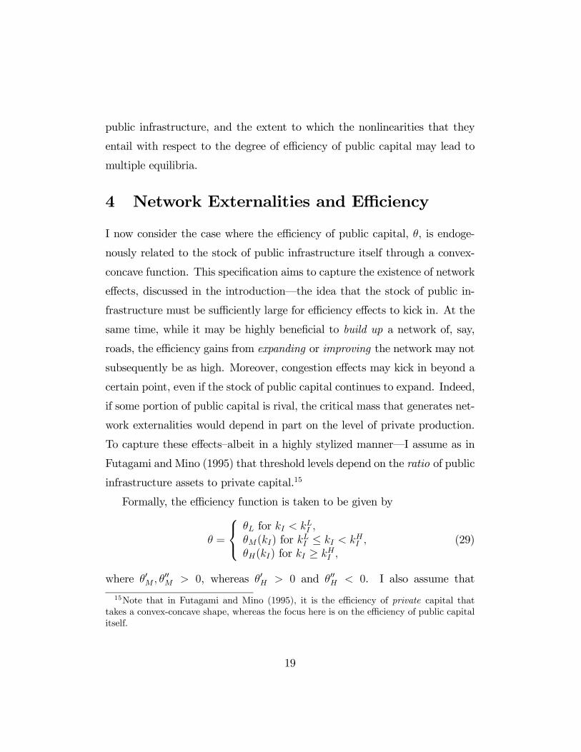
Formally, the efficiency function is taken to be given by

=

⎧⎨⎩ for

() for ≤

() for ≥

(29)

where 0 00 0, whereas 0 0 and 00 0. I also assume that

15Note that in Futagami and Mino (1995), it is the efficiency of private capital that

takes a convex-concave shape, whereas the focus here is on the efficiency of public capital

itself.

19

lim→∞ () = , where .16 Thus, the efficiency function is

constant over the interval (0 ), convex over the interval (

), and con-

cave over the interval ( ∞[. This is depicted in Figure 2, where point corresponds to 00(

) = 00(

) = 0. Put differently, over the interval

( ∞[, the efficiency function has a logistic shape.I assume, as was done earlier, that the household takes as given when

optimizing. Proceeding as before (that is, with the linearized system), and

using the results in the Appendix, the following proposition can be estab-

lished:

Proposition 3. Suppose that the degree of efficiency of public infrastruc-

ture is subject to threshold effects, as described in (29). Depending on the

strength of the efficiency externality, and other model parameters, there may

be either no equilibrium, one equilibrium, or multiple equilibria.

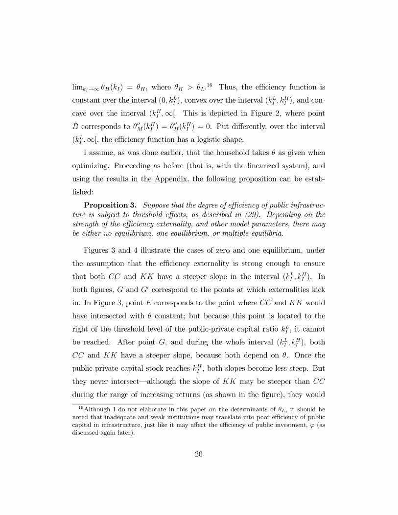
Figures 3 and 4 illustrate the cases of zero and one equilibrium, under

the assumption that the efficiency externality is strong enough to ensure

that both and have a steeper slope in the interval ( ). In

both figures, and 0 correspond to the points at which externalities kick

in. In Figure 3, point corresponds to the point where and would

have intersected with constant; but because this point is located to the

right of the threshold level of the public-private capital ratio , it cannot

be reached. After point , and during the whole interval ( ), both

and have a steeper slope, because both depend on . Once the

public-private capital stock reaches , both slopes become less steep. But

they never intersect–although the slope of may be steeper than

during the range of increasing returns (as shown in the figure), they would

16Although I do not elaborate in this paper on the determinants of , it should be

noted that inadequate and weak institutions may translate into poor efficiency of public

capital in infrastructure, just like it may affect the efficiency of public investment, (as

discussed again later).

20

have intersected at a value higher than ; decreasing returns in efficiency

beyond that threshold value prevents this from happening. Beyond point 0,

curve is shown as steeper than , but no equilibrium can be achieved:

as long as the slope of is flatter than (or, at most, equal to) the slope

of , the two curves cannot intersect.

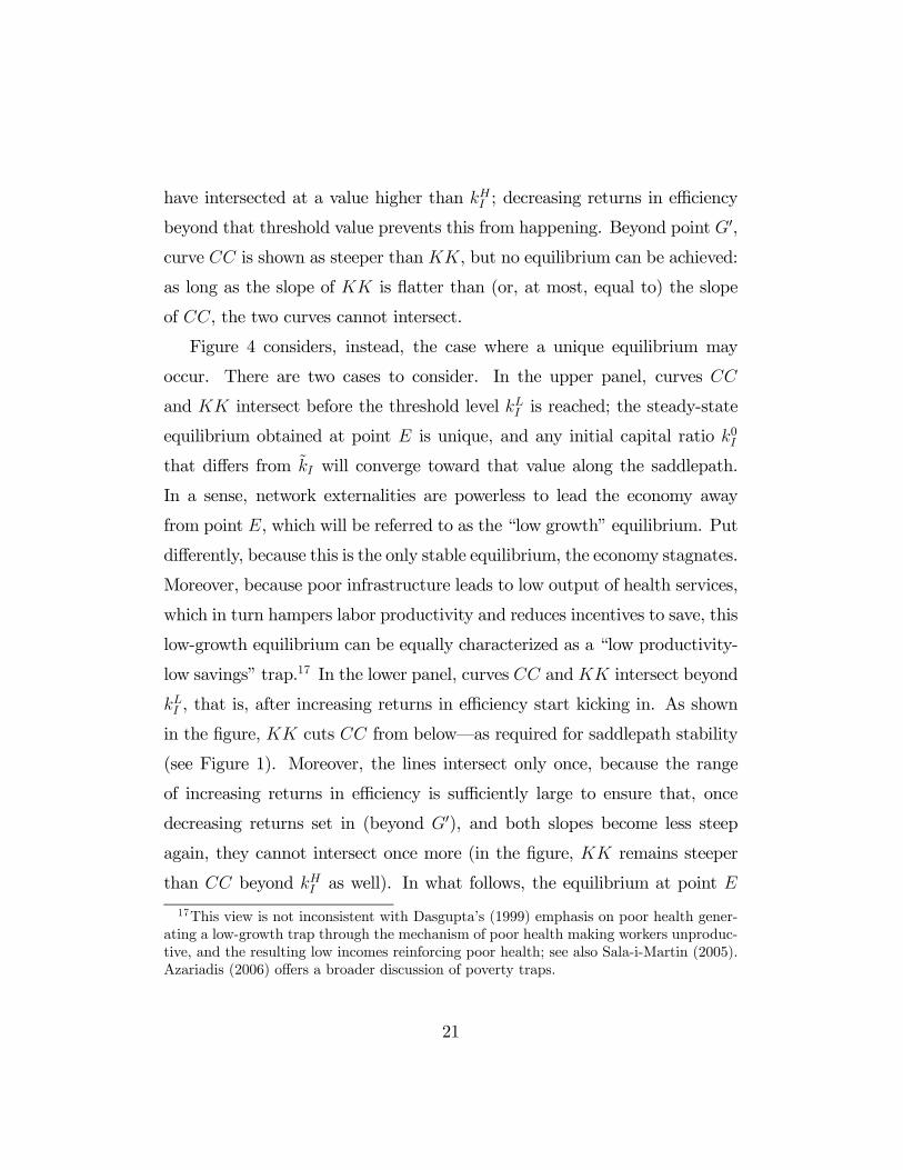
Figure 4 considers, instead, the case where a unique equilibrium may

occur. There are two cases to consider. In the upper panel, curves

and intersect before the threshold level is reached; the steady-state

equilibrium obtained at point is unique, and any initial capital ratio 0

that differs from will converge toward that value along the saddlepath.

In a sense, network externalities are powerless to lead the economy away

from point , which will be referred to as the “low growth” equilibrium. Put

differently, because this is the only stable equilibrium, the economy stagnates.

Moreover, because poor infrastructure leads to low output of health services,

which in turn hampers labor productivity and reduces incentives to save, this

low-growth equilibrium can be equally characterized as a “low productivity-

low savings” trap.17 In the lower panel, curves and intersect beyond

, that is, after increasing returns in efficiency start kicking in. As shown

in the figure, cuts from below–as required for saddlepath stability

(see Figure 1). Moreover, the lines intersect only once, because the range

of increasing returns in efficiency is sufficiently large to ensure that, once

decreasing returns set in (beyond 0), and both slopes become less steep

again, they cannot intersect once more (in the figure, remains steeper

than beyond as well). In what follows, the equilibrium at point

17This view is not inconsistent with Dasgupta’s (1999) emphasis on poor health gener-

ating a low-growth trap through the mechanism of poor health making workers unproduc-

tive, and the resulting low incomes reinforcing poor health; see also Sala-i-Martin (2005).

Azariadis (2006) offers a broader discussion of poverty traps.

21

will be referred to as the “moderate growth” equilibrium.

Consider now the case where multiple equilibria exist. From the results

of the Appendix, the following proposition can be established:

Proposition 4. Suppose that the degree of efficiency of public infrastruc-

ture is subject to threshold effects, as described in (29). If the efficiency ex-

ternality is sufficiently strong, there may be three equilibria. The two extreme

steady states are saddlepoint stable, whereas the intermediate steady state is

unstable.

Figures 5 and 6 illustrate the dynamics in this case.18 The three equilibria

are labeled 1, 2, and 3, with corresponding notation for the steady-state

values of and . As shown in Figure 5, for an economy starting to the

left of 1, or to the right of 1 before point (that is, for 1 0 ),

as well as to the right of 3, or to the left of 3 after point 0 (that is, for

0 3) the realization of a particular equilibrium depends entirely

upon history–that is, the initial value 0 . For instance, an economy whose

initial level of public infrastructure is relatively low, 0 1 , only the low-

growth equilibrium 1 can be attained, whereas an economy whose initial

stock of capital is 0 3 , but with otherwise identical characteristics, will

eventually reach the high-growth equilibrium 3. In both cases, cuts

from below, ensuring saddlepath stability.

If the initial public-private capital ratio lies between and , as shown

in Figure 6, several ranges can be distinguished. Let 1 and 2 be defined

as threshold levels that are such that 1 2 , with¯ − 1

¯and

¯ − 2

¯arbitrarily small. Standard (local) dynamic analysis suggests

therefore that the interval (1 2), which corresponds to points and

0 on

the saddlepaths leading to 1 and 3, respectively, and which includes the

18In principle, it is possible for the model to generate also two equilibria, one stable

and one unstable. However, this is rather unlikely, as suggested by the discussion in the

Appendix.

22

unstable equilibrium 2, defines a zone of indeterminacy. Paths originating

in the interval ( 1) would tend to converge to the low productivity-low

savings trap, 1, whereas paths originating in the interval (2 ) would

tend to converge to the high-growth equilibrium, 3.

By contrast, for any path originating within the interval (1 2), the

economy could go either way: the initial value of is indeterminate for

0 given, so there exists an infinite number of perfect foresight equilibrium

paths–all of which legitimate in the sense that they do not violate the

transversality condition for household’s optimization (equation (26)). In that

interval, “optimistic” expectations (that is, the belief that the economy can

reach the high-growth steady state) could prove self-fulfilling and stir the

economy to the high-growth equilibrium; but because nothing ensures that

expectations can be coordinated in such a way, “pessimistic” expectations

could do as well, and the economy may end up in the low-growth equilib-

rium.19 This is illustrated by the three paths originating from point 2,

under the assumption that 0 = 2 .20 Thus, for some initial values 0 of the

(predetermined) public-private capital ratio, there could be several equilib-

rium trajectories–some leading to stagnation, others to high growth. There

is therefore a coordination problem, which creates a possible role for public

policy–an issue to which I now turn.

19See Matsuyama (1991) for instance for an analysis of the role of self-fulfilling expec-

tations in the development process.20As for instance in Futagami and Mino (1995), it is possible for closed orbits (or limit

cycles) to exist around 2. Indeed, the conditions tr = 0 and det 0, where is the

Jacobian matrix evaluated at 2, imply that the system is unstable and has two purely

imaginary eigenvalues; this result cannot be excluded a priori. However, this is of little

interest in the present context.

23

5 The Role of Public Policy

To illustrate the role of public policy, I first examine the case where, start-

ing from a position of a unique equilibrium (as illustrated in Figure 4) the

government implements as before a budget-neutral increase in the share of

public investment in total infrastructure, financed by a cut in unproductive

expenditure (that is, + = 0). As shown in Figure 7, there are two

cases to consider. In the upper panel, as in Figure 4, the initial equilibrium

occurs at a value of the public-private capital ratio that is less than the lower

threshold level . The increase in , as in Figure 1, shifts line only to

the right. But if this shift is relatively small, the new will still intersect

to the left of , at a point like 0; although the consumption-capital

ratio and the steady-state growth rate eventually increase as a result of the

policy shift, the effect is relatively limited because externalities do no kick in.

By contrast, if the increase in is large enough to shift in such a way

that the point of intersection with occurs to the right of , at a point

like 00, the economy will be in the zone of increasing returns associated with

the efficiency of public capital, and the increase in the consumption-capital

ratio will exceed by an order of magnitude–due to the convexity of in

that range, which implies that both lines have a steeper slope–what would

have been achieved in the absence of network effects. In a manner similar to

Figure 1, if the initial equilibrium is at , the adjustment process will take

the economy through a point such as to point 00.

A similar result obtains in the lower panel of Figure 7, where the initial

steady-state position of the economy is at the “moderate growth” equilibrium

point located to the right of the lower threshold level . If the increase in the

share of public investment in infrastructure is not large, the rightward shift

24

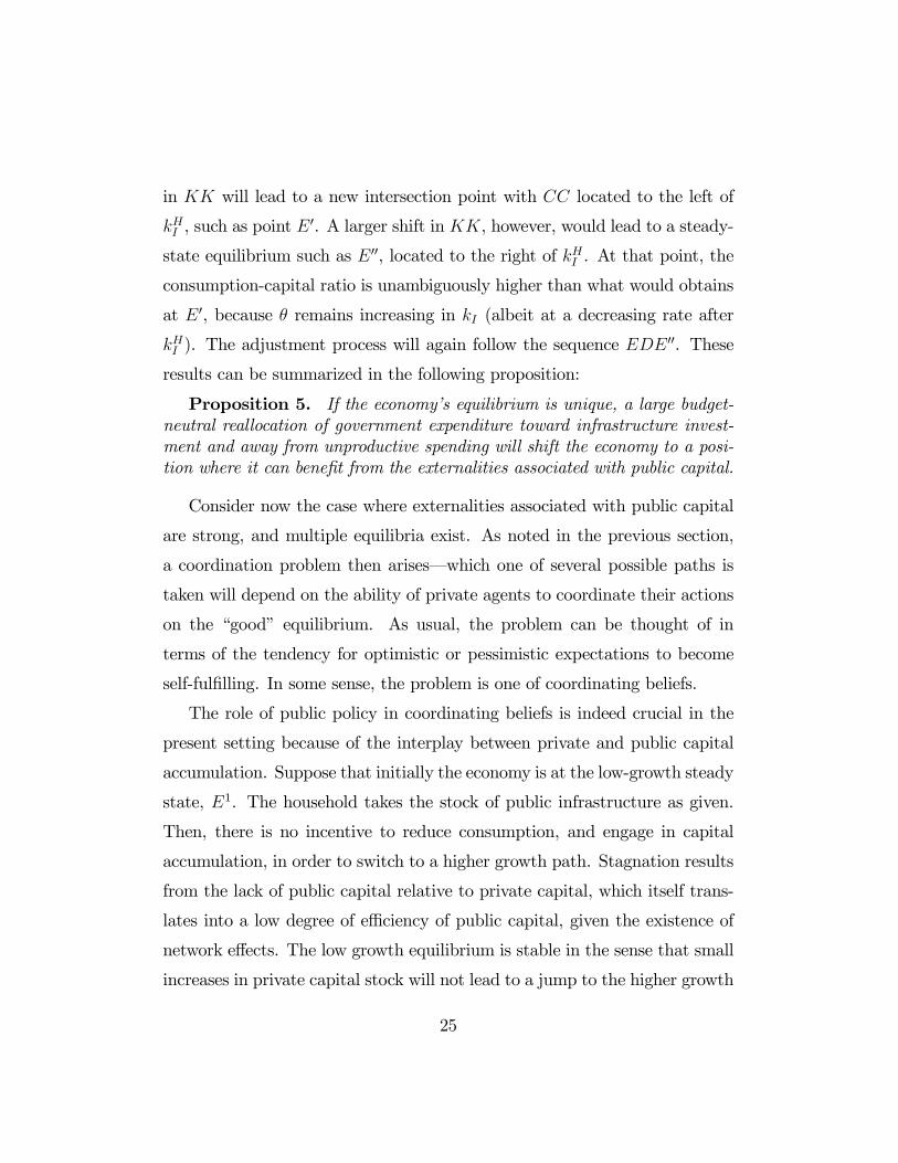
in will lead to a new intersection point with located to the left of

, such as point 0. A larger shift in , however, would lead to a steady-

state equilibrium such as 00, located to the right of . At that point, the

consumption-capital ratio is unambiguously higher than what would obtains

at 0, because remains increasing in (albeit at a decreasing rate after

). The adjustment process will again follow the sequence 00. These

results can be summarized in the following proposition:

Proposition 5. If the economy’s equilibrium is unique, a large budget-

neutral reallocation of government expenditure toward infrastructure invest-

ment and away from unproductive spending will shift the economy to a posi-

tion where it can benefit from the externalities associated with public capital.

Consider now the case where externalities associated with public capital

are strong, and multiple equilibria exist. As noted in the previous section,

a coordination problem then arises–which one of several possible paths is

taken will depend on the ability of private agents to coordinate their actions

on the “good” equilibrium. As usual, the problem can be thought of in

terms of the tendency for optimistic or pessimistic expectations to become

self-fulfilling. In some sense, the problem is one of coordinating beliefs.

The role of public policy in coordinating beliefs is indeed crucial in the

present setting because of the interplay between private and public capital

accumulation. Suppose that initially the economy is at the low-growth steady

state, 1. The household takes the stock of public infrastructure as given.

Then, there is no incentive to reduce consumption, and engage in capital

accumulation, in order to switch to a higher growth path. Stagnation results

from the lack of public capital relative to private capital, which itself trans-

lates into a low degree of efficiency of public capital, given the existence of

network effects. The low growth equilibrium is stable in the sense that small

increases in private capital stock will not lead to a jump to the higher growth

25

steady state. The reason is that, because public investment is financed by

a tax on private output, the supply of public infrastructure is an increasing

function of the private capital stock. Moreover, with limited supply of public

capital, production of health services is low, and the rate of time preference

remains high. Thus, as noted earlier, low savings and labor productivity also

characterize the stagnating equilibrium.

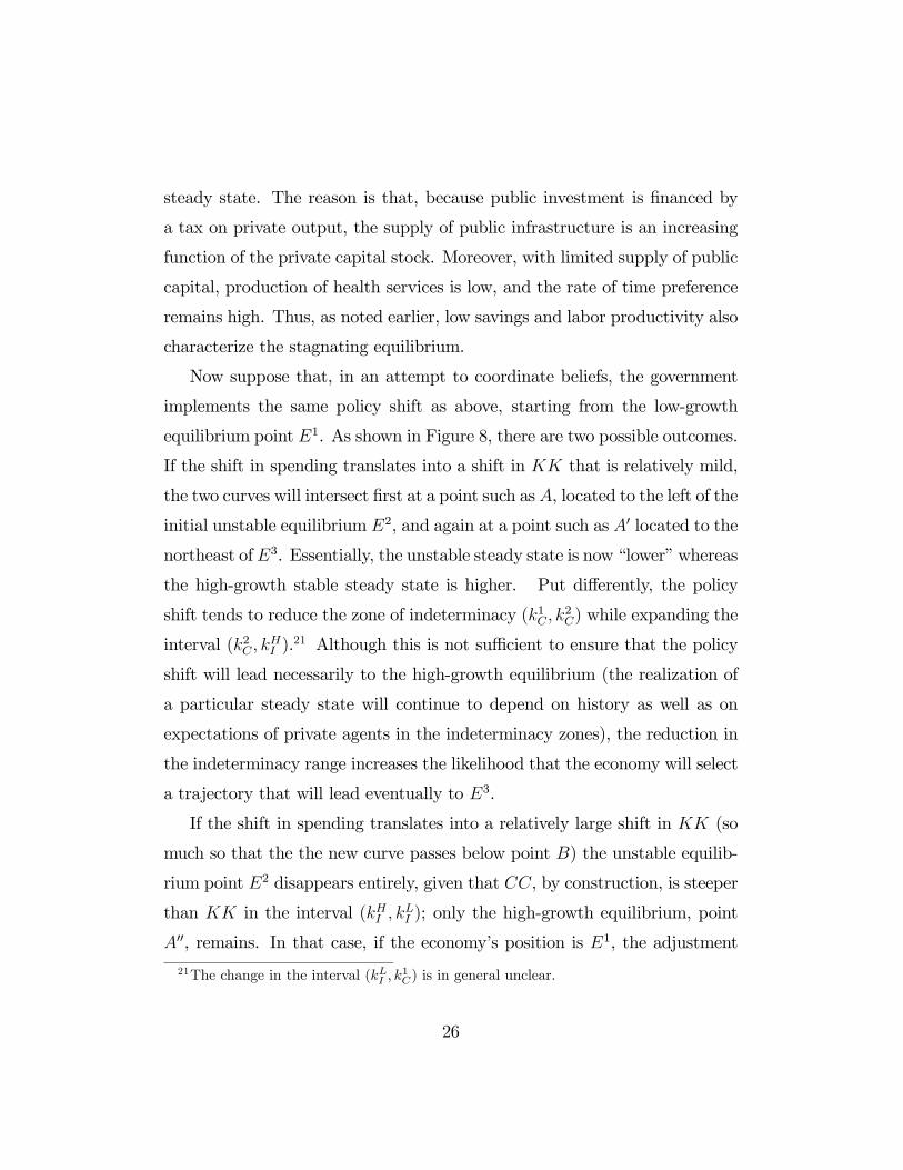
Now suppose that, in an attempt to coordinate beliefs, the government

implements the same policy shift as above, starting from the low-growth

equilibrium point 1. As shown in Figure 8, there are two possible outcomes.

If the shift in spending translates into a shift in that is relatively mild,

the two curves will intersect first at a point such as, located to the left of the

initial unstable equilibrium 2, and again at a point such as 0 located to the

northeast of3. Essentially, the unstable steady state is now “lower” whereas

the high-growth stable steady state is higher. Put differently, the policy

shift tends to reduce the zone of indeterminacy (1 2) while expanding the

interval (2 ).

21 Although this is not sufficient to ensure that the policy

shift will lead necessarily to the high-growth equilibrium (the realization of

a particular steady state will continue to depend on history as well as on

expectations of private agents in the indeterminacy zones), the reduction in

the indeterminacy range increases the likelihood that the economy will select

a trajectory that will lead eventually to 3.

If the shift in spending translates into a relatively large shift in (so

much so that the the new curve passes below point ) the unstable equilib-

rium point 2 disappears entirely, given that , by construction, is steeper

than in the interval ( ); only the high-growth equilibrium, point

00, remains. In that case, if the economy’s position is 1, the adjustment

21The change in the interval ( 1) is in general unclear.

26

path is the same as in Figure 1–on impact the consumption-capital ratio

will jump from 1 to a point such as located on the saddlepath leading to

00. These results can be summarized in the following proposition:

Proposition 6. If there are three steady-state equilibria, a budget-

neutral reallocation of government expenditure toward infrastructure invest-

ment and away from unproductive spending may either reduce the zone of

indeterminacy around the unstable steady state 2 or entirely eliminate it,

thereby increasing the likelihood that the economy will achieve the high-growth

steady state.

In the foregoing discussion, the increase in the share of public expendi-

ture on infrastructure was assumed to be offset by a cut in unproductive

spending. Given the amount of waste that often characterizes public spend-

ing in developing countries, this is not an unreasonable assumption. But a

more general interpretation is also possible, by assuming 0 and by

defining − as foreign aid (that is, grants). Thus, the analysis provides

a theoretical rationale for those who have advocated development strategies

based on large increases in public investment in infrastructure financed by

foreign aid–as for instance in some recent international reports on external

assistance to low-income countries, such as the Millennium Project (2005) of

the United Nations.

My analysis, however, offers a note of caution. In the model, the ability of

a shift in the share of public spending on infrastructure to guide the economy

toward a high growth path is predicated on two critical parameters–the

elasticity of output with respect to public infrastructure, , which determines

the effect of the public capital stock on the marginal product of private

capital; and the degree of efficiency of public investment, , which, as noted

earlier, can be viewed as a broad indicator of the quality of governance. The

lower the values of these two coefficients, the larger the increase in public

27

investment in infrastructure will need to be to generate the shift in

alluded to earlier. The role of is particularly important; weak governance

is often viewed as a chief culprit when assessing why public expenditure often

fails to achieve its intended outcomes.22 Moreover, a negative correlation

could exist between aid and the efficiency parameter , if indeed, as found by

Svensson (2000), aid increases corruption in ethnically divided societies. This

can be stated in the form of the following corollary to the above propositions:

Corollary to Propositions 5 and 6. A large shift in government

expenditure toward infrastructure will generate desirable effects only if the

degree of efficiency of public investment, , is sufficiently high.

A Big Push policy may therefore require concomitant measures to im-

prove governance. Of course, despite past evidence, aid programs themselves

could be structured so as to bring about an increase in efficiency of public

investment–by changing for instance the nature of conditionality in these

programs and making it performance-based, rather than policy-based, and

by allocating a sufficient fraction of aid to capacity building and institutional

reform. If efficiency and governance can indeed be made to depend on aid

itself, the argument for a Big Push in infrastructure investment financed by

external assistance would be strengthened.

Finally, one may ask if results similar to those associated with a shift in

government spending toward infrastructure investment could not be achieved

instead by a shift toward health expenditure, again financed by a cut in

unproductive outlays or foreign aid. After all, spending on health is also

directly productive in this economy, and health services have a direct positive

effect on savings. If the degree of efficiency of investment, , is low, and

22There is no shortage of anecdotal evidence for this in the development literature.

It is also confirmed by a number of recent studies, which show that corruption distorts

incentives to allocate public investment to its initial purpose.

28

the direct effect of public infrastructure on output is somewhat limited, the

economy may well be better off by spending more on health. However, health

services do not generate externalities in the present framework; moreover,

their production requires also infrastructure services. If the parameter

(the elasticity of output of health services with respect to infrastructure) is

relatively large, as suggested by some of the recent studies reviewed in Agénor

(2009b), a strategy based exclusively on the expansion of health services may

not be sufficient to help an economy move to a higher growth path. Of course,

this conjecture is predicated in part on the way health services are modeled in

the present setting. If, for instance, health services are assumed to generate

large positive externalities on labor productivity (with strong convex effects

initially) a case for a “health first” strategy could in principle be viable. The

issue then becomes an empirical one.

6 Concluding Remarks

The purpose of this paper has been to propose a theory of long-run devel-

opment based on public infrastructure as the main engine of growth. In

addition to investing in infrastructure, the government spends on health ser-

vices, which raise labor productivity and lower preference for the present.

The rate of time preference is modeled as a decreasing function of health ser-

vices, relative to the stock of private capital. Agents become less impatient

as their health improves; this, in turn, raises savings and stimulates growth.

In addition, infrastructure affects the production of both commodities and

health services, and therefore labor efficiency.

The first part of the paper described the model and illustrated its func-

tioning by considering a budget-neutral shift in public spending toward in-

29

vestment in infrastructure. This reallocation was shown to raise the steady-

state value of health production, thereby lowering the rate of time preference

and raising savings. This additional savings translates into higher private

capital and consumption in the steady state. Indeed, in the model it is not

only increases in the rate of return on physical capital that leads house-

holds to save more, but also improvements in the consumption of health

services–the supply of which depends on the availability of public capital

in infrastructure. Although the model does not explicitly account for demo-

graphic factors, its prediction that low growth tends to be associated with

low consumption of health services and poor productivity is consistent with

several studies suggesting that health improvements tend to have a large im-

pact on growth. Fogel (1994, 1997) for instance, argued that a significant

fraction of economic growth in Britain during the period 1780-1980 (about

0.33 percent per annum) was due to an increase in effective labor inputs that

resulted from workers’ better nutrition and improved health.23 In the same

vein, Sohn (2000) found that improved nutrition increased available labor

inputs in South Korea by 1 percent a year or more during 1962—95. A num-

ber of other studies have shown that initial levels of life expectancy tend to

have a significant effect on subsequent growth rates (see Agénor (2009a)). In

particular, Lorentzen, McMillan and Wacziarg (2008) found that countries

with a high rate of adult mortality tend to experience low rates of growth–

possibly because when people expect to die relatively young, they have less

incentives to save and invest in the acquisition of skills.24 What the model

23Boucekkine et al. (2003) estimate that a steady decline in adult mortality (while child

mortality stayed level) accounts for 70 percent of the growth acceleration that modern

Europe experienced between 1700 and 1820.24They also found that the estimated effect of high adult mortality on growth is large

enough to explain Africa’s poor economic performance between 1960 and 2000. Indeed, in

the 40 countries with the highest adult mortality rates in their sample of 98 countries, all

30

adds to these studies is that infrastructure may well be one of the main

engines behind the improvement in health outcomes.

In the second part of the paper, it was argued that, as a result of net-

work effects, public infrastructure may generate strong nonconvexity of the

economy’s production technology, with important consequences for the rela-

tionship between public capital and economic growth. As a result of these

effects, the degree of efficiency of public infrastructure becomes nonlinearly

related to the stock of public capital (relative to the private capital stock)

itself. It was shown that, as a result of these nonlinearities, there may be no

equilibrium, a unique equilibrium, or multiple equilibria.

The third part of the paper focused on the role of public policy. It was

shown that if there are three steady-state equilibria, a budget-neutral shift

toward infrastructure investment and away from unproductive spending (or

financed by foreign aid) may either reduce the zone of indeterminacy around

the unstable steady state or entirely eliminate it–if it is large enough. How-

ever, the analysis suggests some caution in the Big Push view recently revived

by Sachs (2005), among others. Sachs emphasizes the lack of savings at low

levels of income as the main cause of a poverty trap.25 This paper suggests

that his analysis is incomplete. In particular, in the present paper a large

shift toward spending on infrastructure will generate desirable effects only if

the degree of efficiency of public investment is sufficiently high. A Big Push

policy may therefore require concomitant measures to improve governance–

possibly by changing the nature and focus of aid conditionality.

The analysis can be extended in several directions. First, greater access to

are in Sub-Saharan Africa, except three.25He also discussed increasing returns (or threshold effects) associated with the capital

stock, but without an explicit formal analysis focusing on public infrastructure, as was

done in the present paper.

31

health services enhances not only workers’ productivity, but also the ability

to learn and accumulate human capital–a significant constraint to growth

in many low-income countries.26 It would therefore be useful to introduce

human capital accumulation and consider its interactions with health. Much

recent evidence suggests that causality goes both ways, as documented for

instance by Agénor (2009b). On the one hand, higher life expectancy in-

creases the payoff from investment in education, thereby raising incentives

to invest in the acquisition of skills. Evidence along these lines (in the form

of a significant effect of life expectancy on years of schooling) is provided

by Acemoglu and Johnson (2007). On the other, a higher level of education

tends to improve health outcomes, in part because it increases awareness of

diseases, both to the individual and their family members (such as moth-

ers teaching their children to wash their hands before preparing and eating

food). In Tamura (2006) for instance, human capital accumulation lowers

mortality, which in turn reduces fertility, thereby inducing a demographic

transition and economic growth–lower fertility reduces the cost of human

capital investment, inducing parents to invest more in the education of their

children. It is not difficult to see in that setting how the lack of infrastructure

can create another source of low-growth trap–poor transportation increases

the time needed to get to school.27 And because the time spent to get to

school raises the total amount of time that must be allocated to acquire skills,

it increases the opportunity cost of education. Given the inability to borrow

for poor households, parents tend to keep children out of school, because they

are unable to cover the upfront cost of schooling (broadly defined to include

26Oketch (2006) found strong evidence that physical capital investment is critical to

human capital accumulation and growth in Sub-Saharan Africa.27The nonlinearity in the “learning curve” defined in Kejak (2003) for instance could be

related to infrastructure.

32

the opportunity cost of not working), in return for future (and uncertain)

benefits. Of course, adding education could lead to additional sources of

nonlinearities; in Mayer-Foulkes (2003, 2005) for instance, the acquisition of

human capital is subject to threshold effects, with threshold levels depending

endogenously on technological change and credit constraints.

Finally, it would be worth exploring another possible externality associ-

ated with infrastructure–regarding not the efficiency of public capital for

a given technology (as was done here), but rather the choice of technology

itself. At low levels of infrastructure, producers may have no choice but

to adopt (or continue to use) a “subsistence” (or inefficient) technology. In

the absence of a reliable power grid, for instance, firms may not be able

to switch to more advanced machines and sophisticated equipment–even

though it would be profitable to do so. With no roads to transport com-

modities between rural and urban areas in a timely fashion, the adoption

of new production techniques in agriculture may not be feasible either. But

once infrastructure provision has reached a certain threshold, producers may

find it easier to adopt a “modern” (or highly productive) technology and

reap the benefits from doing so. This, in turn, would lead to a faster pace of

growth in output and sustained improvements in productivity. Endogeniz-

ing the switch in technology in this way would shed additional light on the

development process while bringing to the fore the critical role of the state

in fostering private sector growth.

33

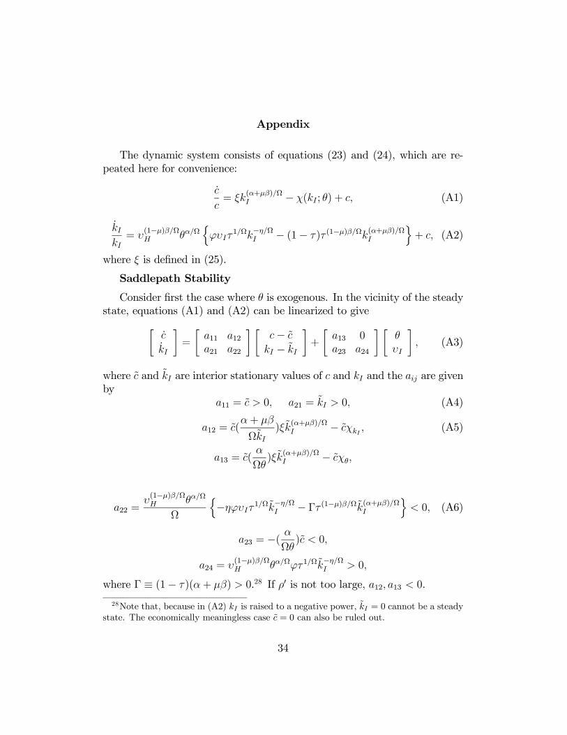
Appendix

The dynamic system consists of equations (23) and (24), which are re-

peated here for convenience:

=

(+)Ω

− ( ; ) + (A1)

=

(1−)Ω Ω

n

1Ω−Ω − (1− ) (1−)Ω(+)Ω

o+ (A2)

where is defined in (25).

Saddlepath Stability

Consider first the case where is exogenous. In the vicinity of the steady

state, equations (A1) and (A2) can be linearized to give∙

¸=

∙11 1221 22

¸ ∙−

−

¸+

∙13 0

23 24

¸ ∙

¸ (A3)

where and are interior stationary values of and and the are given

by

11 = 0 21 = 0 (A4)

12 = (+

Ω)

(+)Ω

− (A5)

13 = (

Ω)

(+)Ω

−

22 =(1−)Ω Ω

Ω

n− 1Ω−Ω − Γ (1−)Ω(+)Ω

o 0 (A6)

23 = −( Ω) 0

24 = (1−)Ω Ω 1Ω

−Ω 0

where Γ ≡ (1− )(+ ) 0.28 If 0 is not too large, 12 13 0.

28Note that, because in (A2) is raised to a negative power, = 0 cannot be a steady

state. The economically meaningless case = 0 can also be ruled out.

34

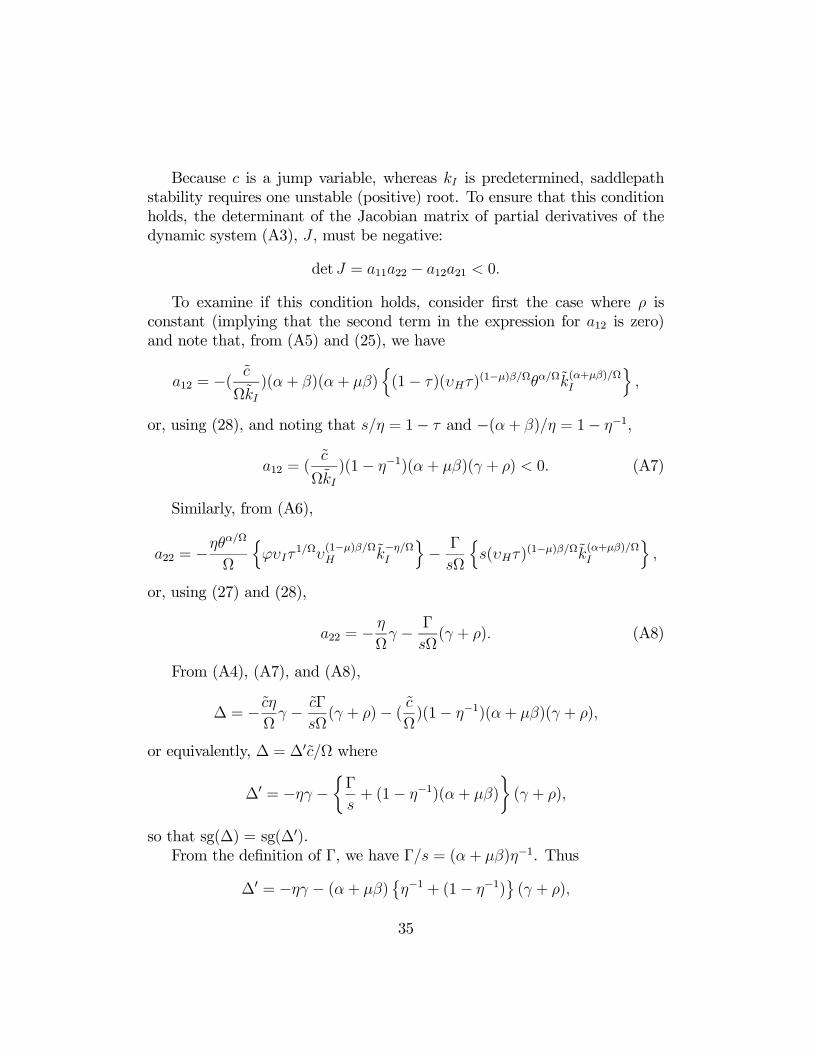
Because is a jump variable, whereas is predetermined, saddlepath

stability requires one unstable (positive) root. To ensure that this condition

holds, the determinant of the Jacobian matrix of partial derivatives of the

dynamic system (A3), , must be negative:

det = 1122 − 1221 0

To examine if this condition holds, consider first the case where is

constant (implying that the second term in the expression for 12 is zero)

and note that, from (A5) and (25), we have

12 = −(

Ω)(+ )(+ )

n(1− )()

(1−)ΩΩ(+)Ω

o

or, using (28), and noting that = 1− and −(+ ) = 1− −1,

12 = (

Ω)(1− −1)(+ )( + ) 0 (A7)

Similarly, from (A6),

22 = −Ω

Ω

n

1Ω(1−)Ω

−Ω

o− Γ

Ω

n()

(1−)Ω(+)Ω

o

or, using (27) and (28),

22 = −

Ω − Γ

Ω( + ) (A8)

From (A4), (A7), and (A8),

∆ = − Ω − Γ

Ω( + )− (

Ω)(1− −1)(+ )( + )

or equivalently, ∆ = ∆0Ω where

∆0 = − −½Γ

+ (1− −1)(+ )

¾( + )

so that sg(∆) = sg(∆0).From the definition of Γ, we have Γ = (+ )−1. Thus

∆0 = − − (+ )©−1 + (1− −1)

ª( + )

35

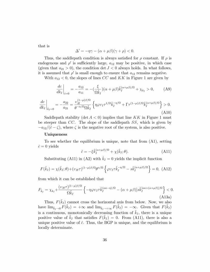
that is

∆0 = − − (+ )( + ) 0

Thus, the saddlepath condition is always satisfied for constant. If is

endogenous and 0 is sufficiently large, 12 may be positive, in which case(given that 21 0), the condition det 0 always holds. In what follows,

it is assumed that 0 is small enough to ensure that 12 remains negative.With 12 0, the slopes of lines and in Figure 1 are given by

¯=0

= −1211

= −(

Ω)(+ )

(+)Ω

+ 0 (A9)

¯=0

= −2221

=(1−)Ω

−ΩΩ

n

1Ω−Ω + Γ (1−)Ω(+)Ω

o 0

(A10)

Saddlepath stability (det 0) implies that line in Figure 1 must

be steeper than . The slope of the saddlepath , which is given by

−12(− ), where is the negative root of the system, is also positive.

Uniqueness

To see whether the equilibrium is unique, note that from (A1), setting

= 0 yields

= −(+)Ω + ( ; ) (A11)

Substituting (A11) in (A2) with = 0 yields the implicit function

() = ( ; )+()(1−)ΩΩ

n

−Ω −

(+)Ω

o= 0 (A12)

from which it can be established that

= +

()(1−)Ω

Ω

n− (−)Ω − (+ )]

[+(+)]Ω

o 0

(A13a)

Thus, () cannot cross the horizontal axis from below. Now, we also

have lim→0 () = +∞ and lim→+∞ () = −∞. Given that ()is a continuous, monotonically decreasing function of , there is a unique

positive value of that satisfies () = 0. From (A11), there is also a

unique positive value of . Thus, the BGP is unique, and the equilibrium is

locally determinate.

36

Effects of an increase in

To establish the effect of an increase in , note that from (A3), we have

| given = 0 and | given = −2421 0. Thus, an increase

in has no effect on curve and shifts curve downward and to the

right in Figure 1. The steady-state effects on and are given by

=

1224

∆ 0

=−1124

∆ 0

which indicate that both and increase.29

Threshold Effects and Multiple Equilibria

Consider now the case where efficiency is subject to threshold effects.

For , and thus constant, stability conditions are those discussed

previously. For , by contrast, = (); to fix ideas, let = 0 ,

where = 1 1 ( = 2 1 1) for the convex (concave) portion of the

curve in Figure 2. The case of constant corresponds therefore to = 0.

For simplicity, I normalize 0 to unity in what follows.

In this case, using (A1) and (25), the steady-state values of and must

satisfy

= ( ; )− 0[+(+)]Ω (A14)

where 0 ≡ −(1− )( + )()(1−)Ω = with = 1. The slope of

is thus given by

¯=0

= + (

)− 0[

+ (+ )

Ω][+(+)]Ω

0

which is steeper than than the case where = 0, under the assumption above

on 0 (which also implies that is not too large); see (A9).Similarly, using (A2) and (25), the steady-state values of and must

satisfy

= Ω

[1(+)Ω

− 2−Ω ] (A15)

where 1 ≡ (1 − )()(1−)Ω 0, and 2 ≡

(1−)Ω

1Ω 0.

To ensure that the consumption-private capital ratio is positive requires

29Equation (A3) can also be used to study the effects of an increase in . Given the

signs of 13 and 23, it can readily be established that the impact on and is in general

ambiguous.

37

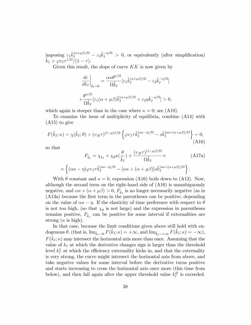
imposing 1(+)Ω

− 2−Ω 0, or equivalently (after simplification)

1Ω(1− ).

Given this result, the slope of curve is now given by

¯=0

=Ω

Ω[1

(+)Ω

− 2−Ω ]

+Ω

Ω[1(+ )

(+)Ω

+ 2−Ω ] 0

which again is steeper than in the case where = 0; see (A10).

To examine the issue of multiplicity of equilibria, combine (A14) with

(A15) to give

( ;) = ( ; ) + ()(1−)Ω

n

(−)Ω −

[+(+)]Ω

o= 0

(A16)

so that

= + (

) +

()(1−)Ω

Ω× (A17a)

×n(− )

(−)Ω − [+ (+ )]

[+(+)]Ω

o

With constant and = 0, expression (A16) boils down to (A12). Now,

although the second term on the right-hand side of (A16) is unambiguously

negative, and + (+ ) 0, is no longer necessarily negative (as in

(A13a) because the first term in the parentheses can be positive, depending

on the value of − . If the elasticity of time preference with respect to

is not too high, (so that is not large) and the expression in parentheses

remains positive, can be positive for some interval if externalities are

strong ( is high).

In that case, because the limit conditions given above still hold with en-

dogenous , (that is, lim→0 ( ;) = +∞, and lim→+∞ ( ;) = −∞), ( ;)may intersect the horizontal axis more than once. Assuming that the

value of at which the derivative changes sign is larger than the threshold

level at which the efficiency externality kicks in, and that the externality

is very strong, the curve might intersect the horizontal axis from above, and

take negative values for some interval before the derivative turns positive

and starts increasing to cross the horizontal axis once more (this time from

below), and then fall again after the upper threshold value is exceeded.

38

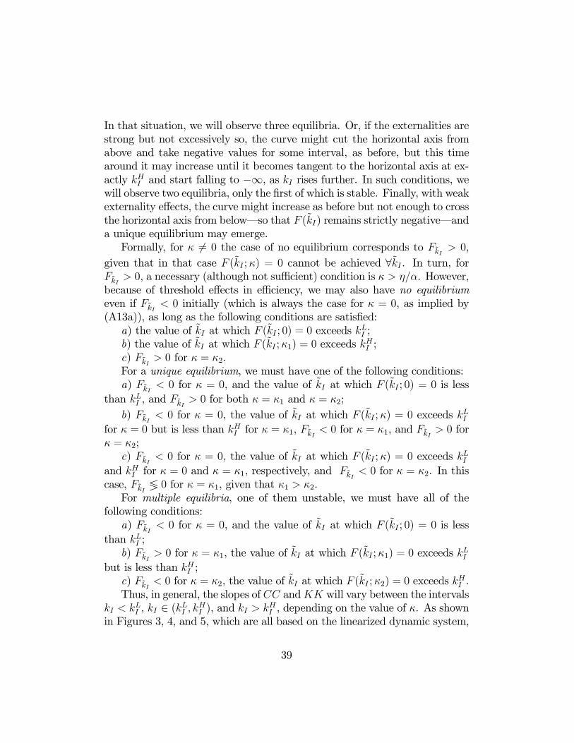
In that situation, we will observe three equilibria. Or, if the externalities are

strong but not excessively so, the curve might cut the horizontal axis from

above and take negative values for some interval, as before, but this time

around it may increase until it becomes tangent to the horizontal axis at ex-

actly and start falling to −∞, as rises further. In such conditions, wewill observe two equilibria, only the first of which is stable. Finally, with weak

externality effects, the curve might increase as before but not enough to cross

the horizontal axis from below–so that () remains strictly negative–and

a unique equilibrium may emerge.

Formally, for 6= 0 the case of no equilibrium corresponds to 0,

given that in that case ( ;) = 0 cannot be achieved ∀ . In turn, for

0, a necessary (although not sufficient) condition is . However,

because of threshold effects in efficiency, we may also have no equilibrium

even if 0 initially (which is always the case for = 0, as implied by

(A13a)), as long as the following conditions are satisfied:

a) the value of at which ( ; 0) = 0 exceeds ;

b) the value of at which ( ;1) = 0 exceeds ;

c) 0 for = 2.

For a unique equilibrium, we must have one of the following conditions:

a) 0 for = 0, and the value of at which ( ; 0) = 0 is less

than , and 0 for both = 1 and = 2;

b) 0 for = 0, the value of at which ( ;) = 0 exceeds

for = 0 but is less than for = 1, 0 for = 1, and

0 for

= 2;

c) 0 for = 0, the value of at which ( ;) = 0 exceeds

and for = 0 and = 1, respectively, and 0 for = 2. In this

case, ≶ 0 for = 1, given that 1 2.

For multiple equilibria, one of them unstable, we must have all of the

following conditions:

a) 0 for = 0, and the value of at which ( ; 0) = 0 is less

than ;

b) 0 for = 1, the value of at which ( ;1) = 0 exceeds

but is less than ;

c) 0 for = 2, the value of at which ( ;2) = 0 exceeds

.

Thus, in general, the slopes of and will vary between the intervals

, ∈ ( ), and , depending on the value of . As shown

in Figures 3, 4, and 5, which are all based on the linearized dynamic system,

39

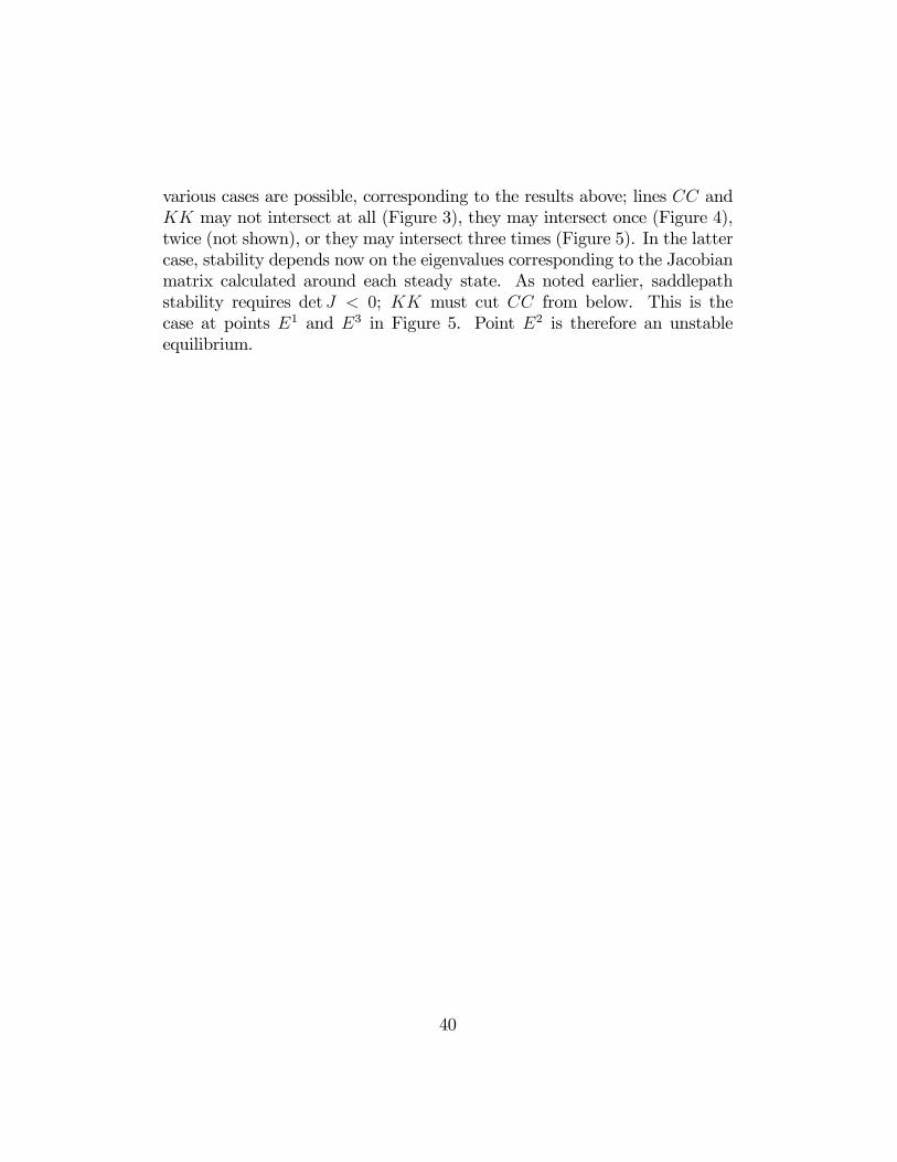
various cases are possible, corresponding to the results above; lines and

may not intersect at all (Figure 3), they may intersect once (Figure 4),

twice (not shown), or they may intersect three times (Figure 5). In the latter

case, stability depends now on the eigenvalues corresponding to the Jacobian

matrix calculated around each steady state. As noted earlier, saddlepath

stability requires det 0; must cut from below. This is the

case at points 1 and 3 in Figure 5. Point 2 is therefore an unstable

equilibrium.

40

References

Acemoglu, Daron, and Simon Johnson, “Disease and Development: The Effect

of Life Expectancy on Economic Growth,” Journal of Political Economy, 115

(December 2007), 925-85.

Agénor, Pierre-Richard, “Health and Infrastructure in a Model of Endogenous

Growth,” Journal of Macroeconomics, 30 (December 2008), 1407-22.

Agénor, Pierre-Richard, “Public Capital, Health Persistence and Poverty Traps,”

Working Paper No. 115, Centre for Growth and Business Cycle Research,

University of Manchester (February 2009a).

––, Public Capital, Growth, and Welfare, book in progress, University of

Manchester (December 2009b).

Agénor, Pierre-Richard, and Peter J. Montiel, Development Macroeconomics,

3rd ed., Princeton University Press (Princeton, New Jersey: 2008).

Agénor, Pierre-Richard, and Kyriakos Neanidis, “The Allocation of Public Ex-

penditure and Economic Growth,”Working Paper No. 69, Centre for Growth

and Business Cycle Research, University of Manchester (March 2006). Forth-

coming, Manchester School of Social and Economic Studies.

Aísa, Rosa, and F. Pueyo, “Government Health Spending and Growth in a Model

of Endogenous Longevity,” Economics Letters, 90 (February 2006), 249-53.

Arestoff, Florence, and Christophe Hurlin, “Threshold Effects in the Productiv-

ity of Public Capital in Developing Countries,” unpublished, University of

Orléans (May 2005).

Azariadis, Costas, “The Theory of Poverty Traps: What Have we Learned?,” in

Poverty Traps, ed. by Samuel Bowles, Steven N. Durlauf, and Karla Hoff,

Princeton University Press (Princeton, New Jersey: 2006).

Bertocchi, Graziella, and Fabio Canova, “Did Colonization Matter for Growth?

An Empirical Exploration into the Historical Causes of Africa’s Underdevel-

opment,” European Economic Review, 46 (December 2002), 1851-71.

Blackburn, Keith, and Giam P. Cipriani, “A Model of Longevity and Growth,”

Journal of Economic Dynamics and Control,” 26 (February 2002), 187-204.

Blanchard, Olivier J., “Debt, Deficits, and Finite Horizons,” Journal of Political

Economy, 93 (April 1985), 223-47.

Blanchard, O. J., Fischer, S., 1989. Lectures on Macroeconomics. MIT Press,

Cambridge, Mass.

Boucekkine, Raouf, David de la Croix, and Omar Licandro, “Early Mortality

Declines at the Dawn of Modern Economic Growth,” Scandinavian Journal

of Economics, 105 (September 2003), 401-18.

41

Buiter, Willem H., “Death, Birth, Productivity Growth and Debt Neutrality,”

Economic Journal, 98 (June 1988), 279-93.

Bunzel, Helle, and Xue Qiao, “Endogenous Lifetime and Economic Growth Re-

visited,” Economics Bulletin, 8 (February 2005), 1-8.

Cazzavillan, Guido, “Public Spending, Endogenous Growth, and Endogenous

Fluctuations,” Journal of Economic Theory, 71 (November 1996), 394-415.

Chakraborty, Shankha, “Endogenous Lifetime and Economic Growth,” Journal

of Economic Theory, 116 (May 2004), 119-37.

Chen, Been-Lon, “Public Capital, Endogenous Growth, and Endogenous Fluc-

tuations,” Journal of Macroeconomics, 28 (December 2006), 768-74.

Cooper, Frederick, “Africa and the World Economy,” in Frederick Cooper, Allen

F. Isaacman, Florencia E. Mallon, and Steve J. Stern, Confronting Historical

Paradigms, University of Wisconsin Press (Madison, Wisconsin: 1993).

Dasgupta, Partha, “Nutritional Status, the Capacity for Work, and Poverty

Traps,” in Labour Markets, Poverty, and Development, ed. by Giorgio Barba

Navaretti, Riccardo Faini, and Giovanni Zanalda, Oxford University Press

(New York: 1999).

Economides, Nicholas, “The Economics of Networks,” International Journal of

Industrial Organization, 14 (October 1996), 669-71.

Ehrlich, Isaac, and Jinyoung Kim, “Endogenous Fertility, Mortality and Eco-

nomic Growth: Can a Malthusian Framework Account for the Conflicting

Historical Trends in Population?,” Journal of Asian Economics, 16 (October

2005), 789-806.

Eicher, T., Turnovsky, S. J., 1999. Non-scale models of endogenous growth.

Economic Journal 109, 394-415.

Epstein, Larry G., and J. Allan Hynes, “The Rate of Time Preference and Dy-

namic Economic Analysis,” Journal of Political Economy, 81 (August 1983),

611-35.

Fernald, John G., “Roads to Prosperity? Assessing the Link between Public

Capital and Productivity,” American Economic Review, 89 (June 1999), 619-

38.

Fogel, Robert W., “Economic Growth, Population Theory, and Physiology: The

Bearing of Long-Term Processes on the Making of Economic Policy,” Amer-

ican Economic Review, 83 (June 1994), 369-95.

––, “New Findings on Secular Trends in Nutrition and Mortality: Some Im-

plications for Population Theory,” in Handbook of Population and Family

Economics, Vol. 1A, ed. by Mark Rosenzweig and Oded Stark (Amsterdam:

1997).

42

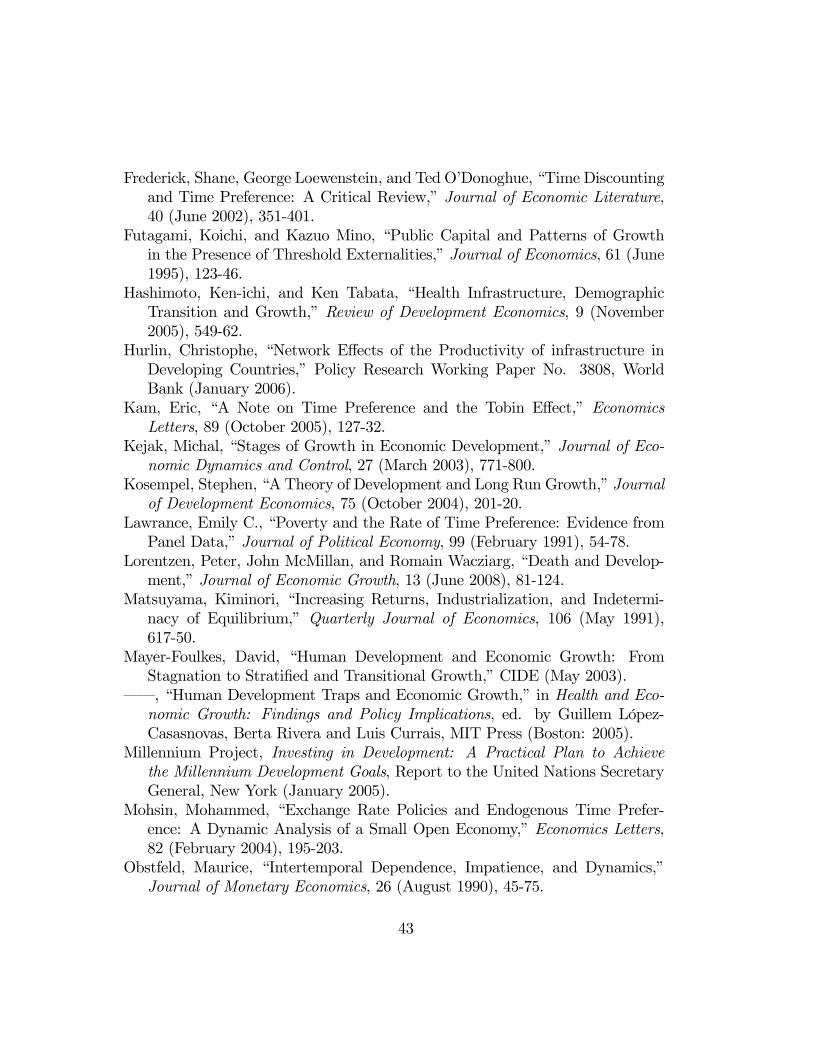
Frederick, Shane, George Loewenstein, and Ted O’Donoghue, “Time Discounting

and Time Preference: A Critical Review,” Journal of Economic Literature,

40 (June 2002), 351-401.

Futagami, Koichi, and Kazuo Mino, “Public Capital and Patterns of Growth

in the Presence of Threshold Externalities,” Journal of Economics, 61 (June

1995), 123-46.

Hashimoto, Ken-ichi, and Ken Tabata, “Health Infrastructure, Demographic

Transition and Growth,” Review of Development Economics, 9 (November

2005), 549-62.

Hurlin, Christophe, “Network Effects of the Productivity of infrastructure in

Developing Countries,” Policy Research Working Paper No. 3808, World

Bank (January 2006).

Kam, Eric, “A Note on Time Preference and the Tobin Effect,” Economics

Letters, 89 (October 2005), 127-32.

Kejak, Michal, “Stages of Growth in Economic Development,” Journal of Eco-

nomic Dynamics and Control, 27 (March 2003), 771-800.

Kosempel, Stephen, “A Theory of Development and Long Run Growth,” Journal

of Development Economics, 75 (October 2004), 201-20.

Lawrance, Emily C., “Poverty and the Rate of Time Preference: Evidence from

Panel Data,” Journal of Political Economy, 99 (February 1991), 54-78.

Lorentzen, Peter, John McMillan, and Romain Wacziarg, “Death and Develop-

ment,” Journal of Economic Growth, 13 (June 2008), 81-124.

Matsuyama, Kiminori, “Increasing Returns, Industrialization, and Indetermi-

nacy of Equilibrium,” Quarterly Journal of Economics, 106 (May 1991),

617-50.

Mayer-Foulkes, David, “Human Development and Economic Growth: From

Stagnation to Stratified and Transitional Growth,” CIDE (May 2003).

––, “Human Development Traps and Economic Growth,” in Health and Eco-

nomic Growth: Findings and Policy Implications, ed. by Guillem López-

Casasnovas, Berta Rivera and Luis Currais, MIT Press (Boston: 2005).

Millennium Project, Investing in Development: A Practical Plan to Achieve

the Millennium Development Goals, Report to the United Nations Secretary

General, New York (January 2005).

Mohsin, Mohammed, “Exchange Rate Policies and Endogenous Time Prefer-

ence: A Dynamic Analysis of a Small Open Economy,” Economics Letters,

82 (February 2004), 195-203.

Obstfeld, Maurice, “Intertemporal Dependence, Impatience, and Dynamics,”

Journal of Monetary Economics, 26 (August 1990), 45-75.

43

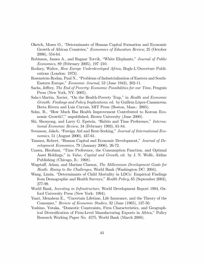
Oketch, Moses O., “Determinants of Human Capital Formation and Economic

Growth of African Countries,” Economics of Education Review, 25 (October

2006), 554-64.

Robinson, James A., and Ragnar Torvik, “White Elephants,” Journal of Public

Economics, 89 (February 2005), 197—210.

Rodney, Walter, How Europe Underdeveloped Africa, Bogle-L’Ouverture Publi-

cations (London: 1973).

Rosenstein-Rodan, Paul N., “Problems of Industrialisation of Eastern and South-

Eastern Europe,” Economic Journal, 53 (June 1943), 202-11.

Sachs, Jeffrey, The End of Poverty: Economic Possibilities for our Time, Penguin

Press (New York, NY: 2005).

Sala-i-Martin, Xavier, “On the Health-Poverty Trap,” in Health and Economic

Growth: Findings and Policy Implications, ed. by Guillem López-Casasnovas,

Berta Rivera and Luis Currais, MIT Press (Boston, Mass.: 2005).

Sohn, B., “How Much Has Health Improvement Contributed to Korean Eco-

nomic Growth?,” unpublished, Brown University (June 2000).

Shi, Shouyong, and Larry G. Epstein, “Habits and Time Preference,” Interna-

tional Economic Review, 34 (February 1993), 61-84.

Svensson, Jakob, “Foreign Aid and Rent-Seeking,” Journal of International Eco-

nomics, 51 (August 2000), 437-61.

Tamura, Robert, “Human Capital and Economic Development,” Journal of De-

velopment Economics, 79 (January 2006), 26-72.

Uzawa, Hirofumi, “Time Preference, the Consumption Function, and Optimal

Asset Holdings,” in Value, Capital and Growth, ed. by J. N. Wolfe, Aldine

Publishing (Chicago, Il.: 1968).

Wagstaff, Adam, and Mariam Claeson, The Millennium Development Goals for

Heath: Rising to the Challenges, World Bank (Washington DC: 2004).

Wang, Limin, “Determinants of Child Mortality in LDCs: Empirical Findings

from Demographic and Health Surveys,” Health Policy, 65 (September 2003),

277-99.

World Bank, Investing in Infrastructure, World Development Report 1994, Ox-

ford University Press (New York: 1994).

Yaari, Menahem E., “Uncertain Lifetime, Life Insurance, and the Theory of the

Consumer,” Review of Economic Studies, 32 (June (1965), 137-50.

Yoshino, Yutaka, “Domestic Constraints, Firm Characteristics, and Geograph-

ical Diversification of Firm-Level Manufacturing Exports in Africa,” Policy

Research Working Paper No. 4575, World Bank (March 2008).

44

Figure 1 Increase in the Share of Spending on Infrastructure Financed by a Cut in Unproductive Spending

S

c

S

K

K

C

C

E'

c~

0kIIk~

E

A

Figure 2 Network Externalities and Endogenous Efficiency

θ

A

0kI

Congestion effects

B

LkIHkI

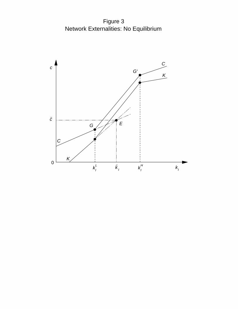
Figure 3Network Externalities: No Equilibrium

c

K

K

C

C

Ec~

0kIIk~ HkI

LkI

G'

G

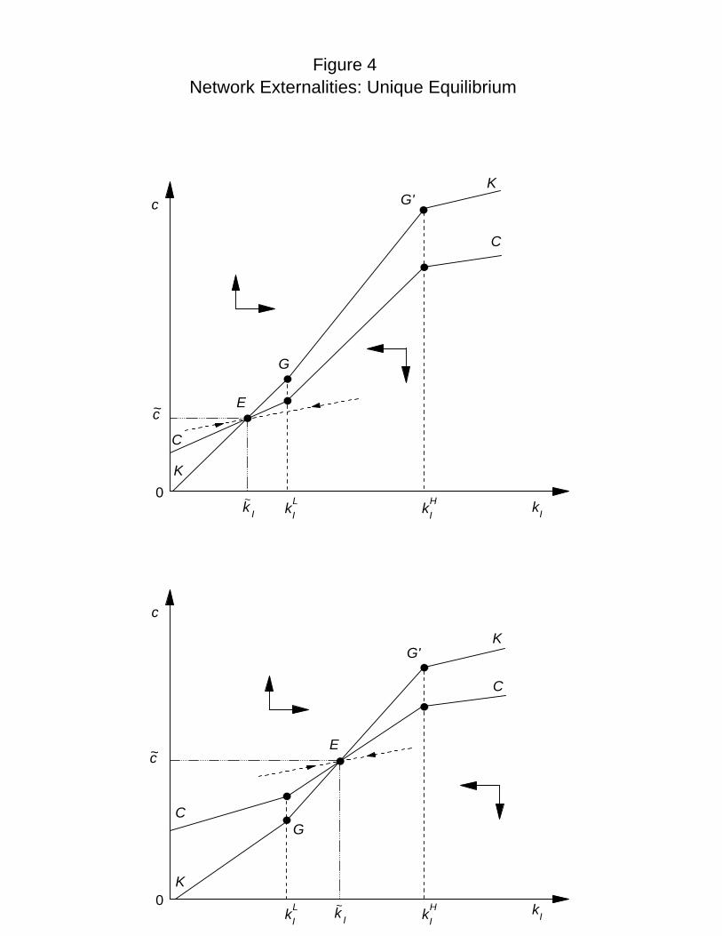
Figure 4

cK

C

C

c~

0

c

K

K

C

C

c~

0

Network Externalities: Unique Equilibrium

kI

kI

HkILkI

G'

G

Ik~

E

E

HkILkI Ik~

G'

G

K

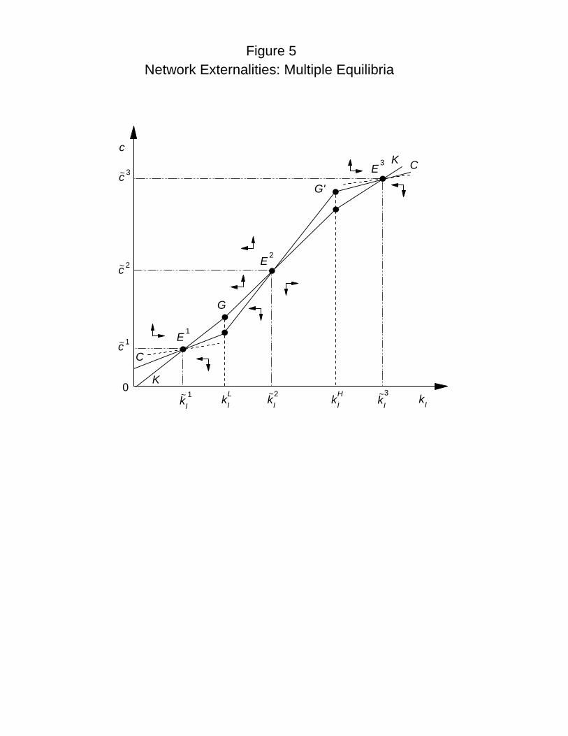
Figure 5 Network Externalities: Multiple Equilibria

c

K

K

C

C

0kI

E 2

E 3

E 1

HkILkIIk~

1Ik~2

Ik~3

c~ 1

c~ 2

c~ 3

G'

G

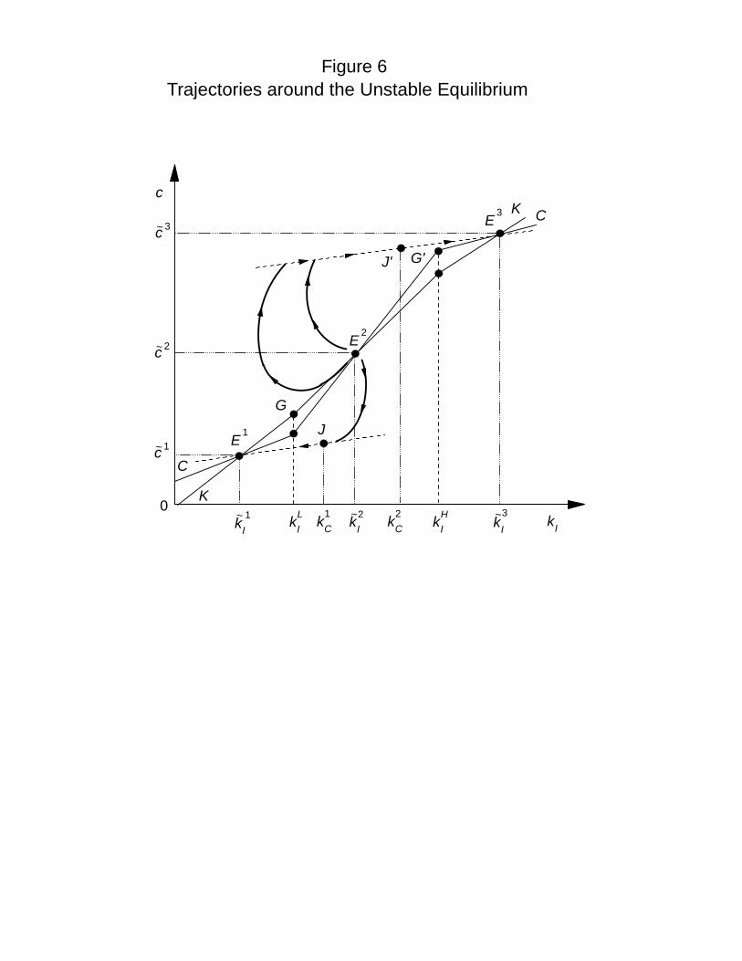
Figure 6

c

K

K

C

C

0kI

E 2

E 3

E 1

HkILkIIk~

1Ik~2

Ik~3

c~ 1

c~ 2

c~ 3

G'

G

Trajectories around the Unstable Equilibrium

kC1 kC

2

J

J'

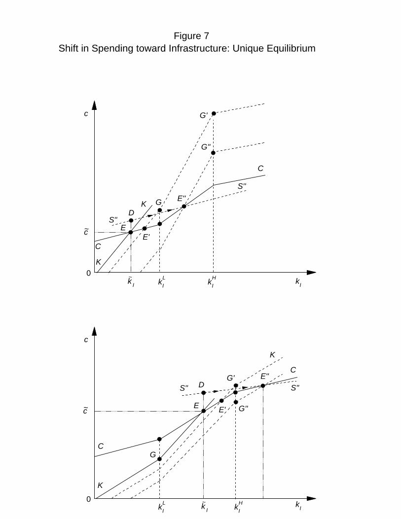
Figure 7

S''

c

S''

K

C

C

c~

0

c

K

K

C

C

c~

0

kI

kI

HkILkI

G'

G

Ik~

E

E

HkILkI Ik~

G'

G

E''

E''

E'

E' G''

G''

Shift in Spending toward Infrastructure: Unique Equilibrium

D

S''S'' D

K

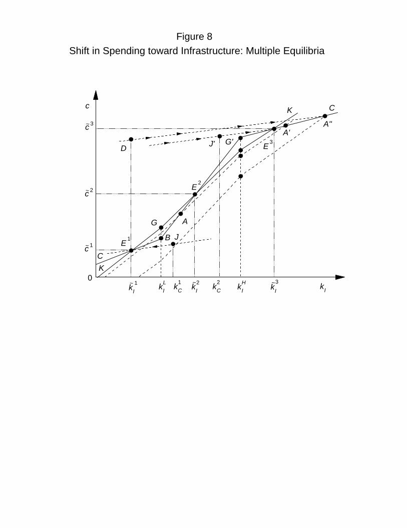
c

K

K

C

C

0kI

E 2

E 3

E 1

HkILkIIk~

1Ik~2

Ik~3

c~ 1

c~ 2

c~ 3

G'

G

kC1 kC

2

J

J'

Figure 8Shift in Spending toward Infrastructure: Multiple Equilibria

A

A'

D

A''

B