Diseño por Estabilidad - SMIE · NTC-ACERO Diseño y Construcción de Estructuras de Acero 2. Diseño por Estabilidad Los estudios para determinar la estabilidad ... En diseño por

NTC-ACERO Diseño y Construcción de Estructuras de Acero

Diseño por Estabilidad

Palacio de Minería – México D.F. 17de septiembre de 2015

CURSO SOBRE ESTRUCTURAS DE ACERO


Literatura sobre Estabilidad Estructural

1.  Galambos and Surovek (2008). Structural stability of steel: concepts and applications for structural engineers. John Wiley and Sons, Inc.

2.  Chen, Lui (1987). Structural Stability: Theory Implementation, Prentice Hall. 3.  Bazant, Cedolin (2010). Stability of Structures: Elastic, Inelastic, Fracture and Damage Theories. 4.  Ziemian (2010). Guide to stability design criteria for metal structures, Wiley. 6th Ed. 5.  Timoshenko, Gere (1963). Theory of elastic stability, McGraw Hill. 6.  Simitses, Hodges (2005). Fundamentals of Structural Stability, Butterworth-Heinemann. 7.  Chen, Lui (1991). Stability Design of Steel Frames, CRC Press.


2. Diseño por Estabilidad

Contenido: 2.1 Disposiciones generales 2.2 Rigidez lateral 2.3 Factor de longitud efectiva y

efectos de esbeltez de conjunto 2.4 Método de análisis por estabilidad 2.5 Método de análisis directo 2.6 Método de la longitud efectiva 2.7 Determinación aproximada

de los efectos de segundo orden



Los estudios para determinar la estabilidad de la estructura, han de incluir: •  Deformaciones axiales, en flexión y en cortante,

de todos los miembros y conexiones, así como cualquier otra deformación que contribuya a los desplazamientos de la estructura

•  Efectos de segundo orden, P∆ y Pδ •  Imperfecciones geométricas •  Reducciones de rigidez debidas a inelasticidad •  Incertidumbres en los valores de rigideces y

resistencias



Efecto: Definición

PΔ

Son los que producen las cargas verticales al actuar sobre la estructura desplazada lateralmente (efectos de conjunto en toda la estructura)

Pδ

Son los ocasionados por las cargas originalmente axiales, cuando actúan sobre el miembro deformado entre sus extremos (Efectos individuales en cada columna)


Métodos de diseño por estabilidad

Concepto Longitud Efectiva Método Directo

Tipo de Análisis Elástico de segundo orden (1)

Elástico de segundo orden (1)

Carga ficticia (2) Ni = 0.003 Wi (o Δo = 0.003L)

Ni = 0.003 Wi (o Δo = 0.003L)

Rigidez efectiva Nominal EI* = EI

EA* = EA

0.8 Nominal: EI* = 0.8 EI

EA* = 0.8 EA Resistencia axial PR con KL (3) PR con L (K=1) Limitaciones I ≤ 0.3 Ninguna (1) Puede realizarse con un método aproximado, iterativo o riguroso. (2) Carga ficticia solo en combinaciones con cargas de gravedad, no se consideran en

cargas que incluyan sismo (3) K = 1 se permite cuando el factor I ≤ 0.08


Índice de estabilidad de un entrepiso

𝐼= ∑↑▒𝑃↓𝑢 𝑄∆↓𝑂𝐻  /𝐿∑↑▒𝐻  

Donde:

ΣPU Fuerza vertical de diseño en el entrepiso en consideración

Q Factor de comportamiento sísmico. En diseño por viento se toma Q=1.0

ΔOH Desplazamiento horizontal relativo de primer orden de los niveles que limitan el entrepiso en consideración, en la dirección de análisis, producido por las fuerzas de diseño

ΣH Suma de todas las fuerzas horizontales de diseño que obran encima del entrepiso en consideración

L Altura del entrepiso


Métodos de análisis de segundo orden

Métodos simplificados: amplifican análisis 1er orden •  Análisis B1-B2 (traslación-impedida y traslación-permitida) •  Análisis modificado •  Análisis separados (gravedad y lateral) •  Amplificación de distorsiones de entrepiso (White 2007)

Métodos iterativos: iteraciones de análisis de 1er orden •  Carga lateral equivalente (Wood et al. 1976) •  Carga de gravedad iterativa (Gaiotti y Smith 1989) •  Rigidez negativa (Rutenberg 1981) Métodos rigurosos: análisis 2º orden directo •  Funciones de estabilidad

•  Ecuaciones pendiente-deflexión [ M = f (θ, Δ) ] •  Matriz de rigidez directa [ K2 ]

•  Matriz de rigidez geométrica [ K2 ] = [ K1 ] + [ Kg ]


2.7. Determinación aproximada de los efectos de segundo orden

Los momentos de segundo orden, se obtienen multiplicando los de primer orden por factores de amplificación:

•  Momentos de diseño en los extremos de las columnas (PΔ):

𝑀↓𝑢𝑜 = 𝑀↓𝑡𝑖 + 𝐵↓2 𝑀↓𝑡𝑝 

•  Momentos de diseño en la zona central de la columna (PΔ y Pδ ):

𝑀↑∗ ↓𝑢𝑜 = 𝐵↓1 (𝑀↓𝑡𝑖 + 𝐵↓2 𝑀↓𝑡𝑝 )

𝐵↓1 = 𝐶𝑚/1− 𝑃↓𝑈 ∕𝐹↓𝑅 𝑃↓𝑒1   

𝐵↓2 = 1/1−1.2𝐼 = 1/1− 1.2𝑄∆↓𝑂𝐻 𝛴𝑃↓𝑈 /𝐿𝛴𝐻   𝐵↓2 = 1/1− 1.2𝑄𝛴𝑃↓𝑈 /𝛴𝑃↓𝑒2    o bien

Cm = 0.6±0.4Mi

M j


Ejemplo – Análisis de 2º orden simplificado

exacting analysis is required. Of course, in those instances, it may be moreappropriate to simply use a direct second-order approach.

8.5.2 Example 8.2: Second-order Amplified Moments

The simple portal frame shown in Figure 8.7 is used in a number of exam-ples throughout the chapter to illustrate the application of the stability provi-sions in the specification. The loads given are the factored loads. We start bydetermining the second-order axial forces and moments in the columns fromthe NT–LT approach using amplification factors B1 and B2. We then com-pare these to the second order forces and moments in the system using adirect second-order analysis.

To begin the NT–LT process, we first analyze the nonsway frame by fix-ing joint C against translation and applying the factored loads as shown inFigure 8.8. After a first-order analysis is run, we record the moments andaxial loads in the columns, as well as the reaction at joint C. The forces andmoments are shown in Table 8.1, and the reaction R ¼ 9:42 kips.

C

D

B

A

w = 2.5 kip/ft.

W21 x 50

H = 4.5k

W10 x 33

30 ft.

18 ft.W10 x 49

Fig. 8.7 Portal frame example.

C

D

B

A

RH = 4.5k

w = 2.5 kip/ft.

Fig. 8.8 NT analysis model.

8.5 SPECIFICATION-BASED APPROACHES FOR STABILITY ASSESSMENT 335

w = 3.72 t/m

9.15 m

5.5

m

V=2 t


Ejemplo – Análisis TI-TP





C

D

B

A

w = 2.5 kip/ft.

W21 x 50

H = 4.5k

W10 x 33

30 ft.

18 ft.W10 x 49


C

D

B

A

RH = 4.5k

w = 2.5 kip/ft.



For the LT analysis, an equal and opposite reaction at C is applied to thesway permitted model of the frame, as shown in Figure 8.9.

One the analyses are complete, we can calculate the B1 and B2 factors.B1 is given by

B1 ¼Cm

1" aPr

Pe1

# 1:0

where

Cm ¼ 0:6" 0:4M1

M2

! "¼ 0:6" 0:4 $ 0

303:8

! "¼ 0:6

and

Pe1 ¼p2EI

ðK1LÞ2¼ p2 $ ð29; 000Þð272Þ½ð1:0Þð18Þð12Þ(2

¼ 1;670 kips ðusing K1 ¼ 1:0Þ

For column AB

Pr ¼ Pnt þ Plt ¼ "40:5þ 5:7 ¼ 34:8 kips

B1 ¼0:6

1" ð1:0Þ34:8

1670

¼ 0:61!B1 ¼ 1:0

C

D

B

A

R = 9.42k

Fig. 8.9 LT analysis model.

TABLE 8.1 NT–LT Analysis Results

NT Analysis LT Analysis

PNT MNT PLT MLT

(kip) (in-kip) (kip) (in-kip)

Col AB "40:5 "1; 063 5.7 2035

Col CD "34:5 0 "5:7 0

336 SPECIFICATION-BASED APPLICATIONS OF STABILITY IN STEEL DESIGN

For the LT analysis, an equal and opposite reaction at C is applied to thesway permitted model of the frame, as shown in Figure 8.9.

One the analyses are complete, we can calculate the B1 and B2 factors.B1 is given by

B1 ¼Cm

1" aPr

Pe1

# 1:0

where

Cm ¼ 0:6" 0:4M1

M2

! "¼ 0:6" 0:4 $ 0

303:8

! "¼ 0:6

and

Pe1 ¼p2EI

ðK1LÞ2¼ p2 $ ð29; 000Þð272Þ½ð1:0Þð18Þð12Þ(2

¼ 1;670 kips ðusing K1 ¼ 1:0Þ

For column AB

Pr ¼ Pnt þ Plt ¼ "40:5þ 5:7 ¼ 34:8 kips

B1 ¼0:6

1" ð1:0Þ34:8

1670

¼ 0:61!B1 ¼ 1:0

C

D

B

A

R = 9.42k

Fig. 8.9 LT analysis model.

TABLE 8.1 NT–LT Analysis Results

NT Analysis LT Analysis

PNT MNT PLT MLT


Col AB "40:5 "1; 063 5.7 2035

Col CD "34:5 0 "5:7 0


A value of B1 < 1 indicates that no amplification of the MNT moment isrequired.

Next, we determine the second-order amplification of the sway momentsby calculating

B2 ¼1

1" aP

PNTPPe2

# 1:0; where a ¼ 1:0 ðfactored loading usedÞ

XPNT ¼ ð40:5þ 35:5Þ ¼ 75 kips

XPe2 ¼

X p2EI

ðK2LÞ2¼ RM

PHL

DH

where Rm ¼ 0:85 for moment framesUsing the second form of the

PPe2 equation based on the LT analysis

results, where DH ¼ 5:87 in:

XPe2 ¼

PHL

DH¼ 0:85ð9:42Þð18

0Þð1200=ft:Þ

5:8700¼ 295 kips

B2 ¼1

1" 75

295

¼ 1:34

The final forces are given by

Mr ¼ B1Mnt þ B2Mlt

Pr ¼ Pnt þ B2Plt

and are tabulated in Table 8.2, where it can be seen that, in this case, theycompare conservatively to the direct second-order elastic analysis results.

TABLE 8.2 Second-order Moment and Axial Load Values

B1-B2 Analysis Second-order Analysis

Pr Mr Pr Mr


Col AB "33:4 1664 "33 1534

Col CD "42:1 0 "42 0


TI TP

Análisis TI Análisis TP

w = 3.72 t/m V=2 t

14.97 cm

R=4.27 t

k=R/∆ =28.66t/m

-147 t-m 281.35 t-m

PTI (t)

MTI (t-m)

PTP (t)

MTP (t-m)

-18.4 t -15.6 t

+2.6 t -2.6 t

K ≤ 1.0


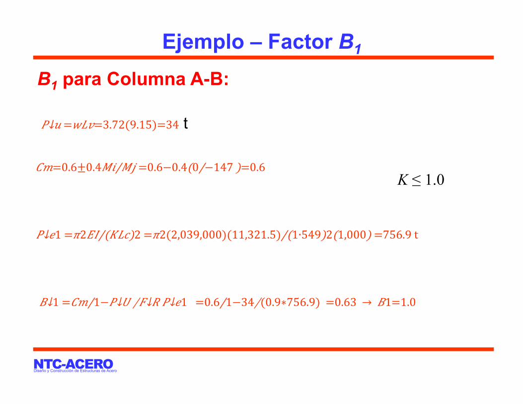
Ejemplo – Factor B1 B1 para Columna A-B:

𝐵↓1 = 𝐶𝑚/1− 𝑃↓𝑈 ∕𝐹↓𝑅 𝑃↓𝑒1   = 0.6/1− 34∕(0.9∗756.9)  =0.63 → 𝐵1=1.0

𝐶𝑚=0.6±0.4𝑀𝑖/𝑀𝑗 =0.6−0.4(0/−147 )=0.6

𝑃↓𝑒1 = 𝜋2𝐸𝐼/(𝐾𝐿𝑐)2 = 𝜋2(2,039,000)(11,321.5)/(1∙549)2(1,000) =756.9 t

𝑃↓𝑢 =𝑤𝐿𝑣=3.72(9.15)=34 t

K ≤ 1.0


Ejemplo – Factor B2 y momento de 2o orden

𝐵↓2 = 1/1−1.2𝐼 = 1/1−1.2(0.22) =1.35

B2 para Columna A-B: 𝐼= ∑↑▒𝑃↓𝑢 𝑄∆↓𝑂𝐻  /𝐿∑↑▒𝐻  = 34(1)/550 14.97/4.27 =0.2167

𝑀↓𝑢𝑜 = 𝑀↓𝑡𝑖 + 𝐵↓2 𝑀↓𝑡𝑝 =−147+1.35(281.35)=𝟐𝟑𝟑 𝐭∙𝐦

𝑀↑∗ ↓𝑢𝑜 = 𝐵↓1 (𝑀↓𝑡𝑖 + 𝐵↓2 𝑀↓𝑡𝑝 )=1(233)=233 t∙m

Momento de segundo orden en Col. AB


Ejemplo – Momento en columna AB

Análisis de segundo orden Simplificado TI-TP vs. Riguroso

𝑀↓𝑢 =134.4 t∙m

𝑀↓𝑢𝑜 /𝑀↓𝑢  = 233/134.4 =1.73

𝑀↓𝑢𝑜 =233 t∙m ( Error = 9.9% )

Análisis de primer orden

𝑀↓𝑢𝑜 =212 t∙m

𝑀↓𝑢𝑜 /𝑀↓𝑢  = 212/134.4 =1.58


Métodos de diseño por estabilidad

Concepto Longitud Efectiva Método Directo

Tipo de Análisis Elástico de segundo orden (1)

Elástico de segundo orden (1)

Carga ficticia (2) Ni = 0.003 Wi (o Δo = 0.003L)

Ni = 0.003 Wi (o Δo = 0.003L)

Rigidez efectiva Nominal EI* = EI

EA* = EA

0.8 Nominal: EI* = 0.8 EI

EA* = 0.8 EA Resistencia axial PR con KL (3) PR con L (K=1) Limitaciones I ≤ 0.3 Ninguna (1) Puede realizarse con un método aproximado, iterativo o riguroso. (2) Carga ficticia solo en combinaciones con cargas de gravedad, no se consideran en

cargas que incluyan sismo (3) K = 1 se permite cuando el factor I ≤ 0.08


Tolerancias Código de Practicas Generales

118

(a) AISC Code of Standard Practice (AISC, 2005d) (b) ACI-117 (2006)

Figure 5.1. Column tolerances as specified in the AISC and the ACI Specifications

Thus, nominal compression capacity of a CFT column (Pn) can be calculated as:

0.658 / 2.25

0.877 / 2.25

o

e

PP

o o en

e o e

P if P PP

P if P P

§ ·° d¨ ¸¨ ¸ ® © ¹°

!¯

(5.1)

(I2-2, I2-3, AISC-10)

The cross-section compressive strength (Po) and the Euler load (Pe) are computed by:

� �2 ' for compact sections

0.7 ' for non-compact sectionss y r yr c c

os cr c c sr s c

A F A F C A fP

A F f A A E E� �

� �

(5.2)

(I2-9, AISC-10)

2

2( )eff

e

EIP

KLS

(5.3)

(I2-5, AISC-10)

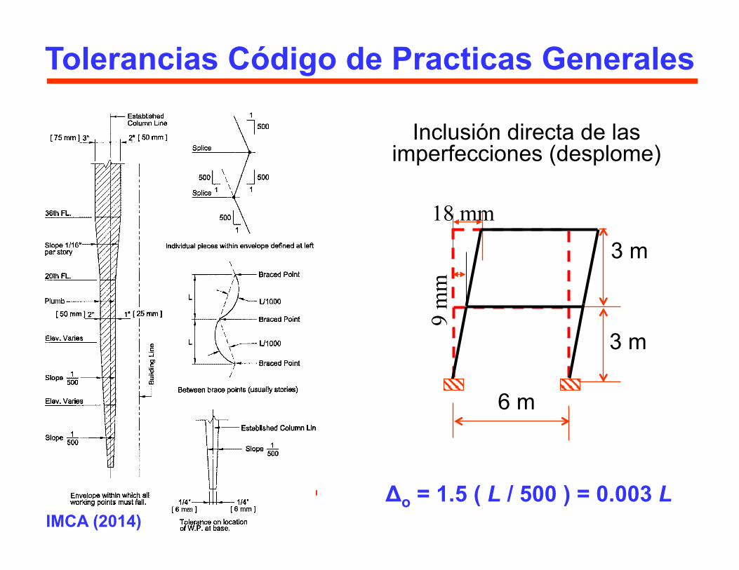
Inclusión directa de las imperfecciones (desplome)

3 m

6 m

3 m

9 m

m

18 mm

Δo = 1.5 ( L / 500 ) = 0.003 L IMCA (2014)


Imperfecciones iniciales *

Inclusión directa de las imperfecciones (desplome)

3 m

6 m

3 m

9 m

m

18 mm

3 m

6 m

3 m

0.12 t

0.09 t

Ni = 0.003 Wi Δo = 0.003 L

Fuerzas ficticias

15 t 15 t

20 t 20 t

* Solo en combinaciones sin carga lateral


Métodos para determinar K

§  Análisis de carga crítica ( Pcr = PeK = Pe / K2 ) §  Ecuaciones teóricas simplificadas

(ojo: hay hipótesis que no siempre se cumplen) §  Sin corrección §  Con corrección (por hipótesis que no se cumplen)

§  Nomogramas (Julian-Lawrence 1959) §  Ecuaciones semi-empíricas aproximadas §  Metodologías para el pandeo de entrepisos:

§  Método de rigidez del entrepiso (LeMessurier 1976) §  Método de pandeo del entrepiso (Yura 1971) §  Método de LeMessurier


important to note that neither of these values for K2 should be used incalculation Pe2 to determine B2.

8.6.6 Example 8.4 Effective Length Calculation with LeanerColumn

Reconsidering the frame in Figure 8.7, we determine the K-factor for col-umn AB. For this frame, we consider three possible variations from the as-sumptions built into the alignment chart:

1. The behavior is purely elastic.

2. All joints are rigid.

3. For columns in sidesway inhibited frames, rotations at opposite endsof the restraining beams are equal in magnitude and opposite in di-rection, producing single curvature bending.

From Example 8.3, we know that Pr ¼ 33k, so we can check whether aninelastic stiffness reduction factor is applicable

aPr

fc

! "

ðFyAgÞ¼

1:0ð33Þ0:9

! "

50ð14:4Þ¼ 0:051 $ 0:39

therefore, t ¼ 1:0, and no inelastic stiffness reduction is applied.The pinned joint at C requires the length of the beam to be modified be-

fore using the alignment chart approach:

L0g ¼ Lg 2%MF

MN

! "¼ 30 2% 0

77:76

! "¼ 600

Next we calculate the sway K-factor:

Gtop ¼

P taI

L

! "

cP I

L

! "

g

¼

1:0ð272Þ18

! "

984

60

! " ¼ 0:92

Gbottom ¼ 10:0ðpinned-endÞ

From alignment charts with Gtop ¼ 0:92 and Gbottom ¼ 10:0, we obtain

Kxffi 1:9


important to note that neither of these values for K2 should be used incalculation Pe2 to determine B2.

8.6.6 Example 8.4 Effective Length Calculation with LeanerColumn

Reconsidering the frame in Figure 8.7, we determine the K-factor for col-umn AB. For this frame, we consider three possible variations from the as-sumptions built into the alignment chart:

1. The behavior is purely elastic.

2. All joints are rigid.

3. For columns in sidesway inhibited frames, rotations at opposite endsof the restraining beams are equal in magnitude and opposite in di-rection, producing single curvature bending.

From Example 8.3, we know that Pr ¼ 33k, so we can check whether aninelastic stiffness reduction factor is applicable

aPr

fc

! "

ðFyAgÞ¼

1:0ð33Þ0:9

! "

50ð14:4Þ¼ 0:051 $ 0:39

therefore, t ¼ 1:0, and no inelastic stiffness reduction is applied.The pinned joint at C requires the length of the beam to be modified be-

fore using the alignment chart approach:

L0g ¼ Lg 2%MF

MN

! "¼ 30 2% 0

77:76

! "¼ 600

Next we calculate the sway K-factor:

Gtop ¼

P taI

L

! "

cP I

L

! "

g

¼

1:0ð272Þ18

! "

984

60

! " ¼ 0:92

Gbottom ¼ 10:0ðpinned-endÞ

From alignment charts with Gtop ¼ 0:92 and Gbottom ¼ 10:0, we obtain

Kxffi 1:9


Ejemplo: Factor K de Columna AB

The K-value can be calculated more accurately using the transcendentalequation that defines the sway-permitted alignment chart

p

K

tanp

K

! "!

p

K

! "2ð10Þð0:95Þ ! 36

6ð10:95Þ ¼ 0

which gives a value of Kx ¼ 1:89.This initial value of Kx must be adjusted to account for the leaning col-

umn, column CD. This can be done using either the story-stiffness or thestory-buckling approach in the commentary. Using story stiffness, where K2

is given by

K2 ¼

ffiffiffiffiffiffiffiffiffiffiffiffiffiffiffiffiffiffiffiffiffiffiffiffiffiffiffiffiffiffiffiffiffiffiffiffiffiffiffiffiffiffiffiffiffiffiffiffiffiffiffiffiffiffiffiffiffiffiffiffiffiffiffiffiffiffiffiffiffiffiffiffiffiPPr

ð0:85þ 0:15RLÞPr

p2EI

L2

$ %DHP

HL

$ %s

The ratio DHPHL

was previously calculated to find B2 in Example 8.2.

DHPHL¼ 1

Pe2¼ 1

295¼ 0:0034

The termP

Pr is the summation of the total axial load on all columns in thestory.

XPr ¼ 75 kips

RL ¼P

Pr leaning columnsPPr all column

¼ 42 kips

75 kips¼ 0:56

K2 ¼


ð0:85þ 0:15RLÞPr

p2EI

L2

$ %DHP

HL

$ %s

¼

ffiffiffiffiffiffiffiffiffiffiffiffiffiffiffiffiffiffiffiffiffiffiffiffiffiffiffiffiffiffiffiffiffiffiffiffiffiffiffiffiffiffiffiffiffiffiffiffiffiffiffiffiffiffiffiffiffiffiffiffiffiffiffiffiffiffiffiffiffiffiffiffiffiffiffiffiffiffiffiffiffiffiffiffiffiffiffiffiffiffiffiffiffiffiffiffiffiffiffiffiffiffiffi75

ð0:85þ 0:15ð0:56ÞÞ33

p2ð29;000Þð272Þð18& 12Þ2

!&0:0034

'vuut ¼ 3:7

8.6 EFFECTIVE LENGTH FACTORS, K-FACTORS 353


p

K

tanp

K

! "!

p

K

! "2ð10Þð0:95Þ ! 36

6ð10:95Þ ¼ 0



is given by

K2 ¼


ð0:85þ 0:15RLÞPr

p2EI

L2

$ %DHP

HL

$ %s

The ratio DHPHL


DHPHL¼ 1

Pe2¼ 1

295¼ 0:0034

The termP


XPr ¼ 75 kips

RL ¼P


¼ 42 kips

75 kips¼ 0:56

K2 ¼


ð0:85þ 0:15RLÞPr

p2EI

L2

$ %DHP

HL

$ %s

¼


ð0:85þ 0:15ð0:56ÞÞ33

p2ð29;000Þð272Þð18& 12Þ2

!&0:0034

'vuut ¼ 3:7

8.6 EFFECTIVE LENGTH FACTORS, K-FACTORS 353The K-factor calculated by the story-buckling approach is given by

K2 ¼

ffiffiffiffiffiffiffiffiffiffiffiffiffiffiffiffiffip2EI

L2

" #

Pr

vuuut PPr

P p2EI

ðKn2LÞ2

!

0

BBBB@

1

CCCCA¼

ffiffiffiffiffiffiffiffiffiffiffiffiffiffiffiffiffiffiffiffiffiffiffiffiffiffiffiffiffiffiffiffiffiffiffiffiffiffiffiffiffiffiffiffiffiffiffiffiffiffiffiffiffiffiffiffiffiffiffiffiffiffiffiffiffiffiffiffiffiffiffiffiffiffiffiffiffip2ð29000Þð272Þð2162Þ

!

33

75

p229000ð272Þð1:95ð216ÞÞ2

!

vuuuuuuut

¼

ffiffiffiffiffiffiffiffiffiffiffiffiffiffiffiffiffiffiffiffiffiffiffið1:95Þ2ð75Þ

33

s

¼ 2:94

Based on an elastic buckling analysis of the frame, the elastic critical buck-ling load, Pcr ¼ 165 kips, and the actual K-factor for column, is given by

K ¼ffiffiffiffiffiffiPe

Pcr

r¼


L2

" #

Pcr

vuuut¼

ffiffiffiffiffiffiffiffiffiffiffi1669

165:3

r¼ 3:18

The actual value lies between the calculated story-stiffness and story-buckling values.

8.7 DESIGN ASSESSMENT BY TWO APPROACHES

In this section, we compare the direct-analysis approach to the critical loador K-factor approach using the portal frame introduced in Example 8.2. Inthis example, we cannot use the first-order approach because the B2 factor(calculated in Example 8.2) is greater than 1.1. While D2=D1 and B2 are notthe exact same value (drift amplification versus moment amplification), B2 isallowed as an approximation of the drift ratio.

8.7.1 Critical Load Approach

In order to perform the strength check, we use the results of Example 8.2with the B1 and B2 amplifiers and the K-factor values determined in Exam-ple 8.4. For this example, we assume the frame is braced in the out-of-planedirection. We check the sidesway stability of the frame by checking the lat-eral resisting member, Column AB. As with the previous example, we focuson the factored lateral load case. The steps are provided in section 8.5.3:

Step 1: Verify that the second- to first-order drift ratio for all stories is lessthan 1.5.






C

D

B

A

w = 2.5 kip/ft.

W21 x 50

H = 4.5k

W10 x 33

30 ft.

18 ft.W10 x 49


C

D

B

A

RH = 4.5k

w = 2.5 kip/ft.



Gb = 10


p

K

tanp

K

! "!

p

K

! "2ð10Þð0:95Þ ! 36

6ð10:95Þ ¼ 0



is given by

K2 ¼


ð0:85þ 0:15RLÞPr

p2EI

L2

$ %DHP

HL

$ %s

The ratio DHPHL


DHPHL¼ 1

Pe2¼ 1

295¼ 0:0034

The termP


XPr ¼ 75 kips

RL ¼P


¼ 42 kips

75 kips¼ 0:56

K2 ¼


ð0:85þ 0:15RLÞPr

p2EI

L2

$ %DHP

HL

$ %s

¼


ð0:85þ 0:15ð0:56ÞÞ33

p2ð29;000Þð272Þð18& 12Þ2

!&0:0034

'vuut ¼ 3:7



p

K

tanp

K

! "!

p

K

! "2ð10Þð0:95Þ ! 36

6ð10:95Þ ¼ 0



is given by

K2 ¼


ð0:85þ 0:15RLÞPr

p2EI

L2

$ %DHP

HL

$ %s

The ratio DHPHL


DHPHL¼ 1

Pe2¼ 1

295¼ 0:0034

The termP


XPr ¼ 75 kips

RL ¼P


¼ 42 kips

75 kips¼ 0:56

K2 ¼


ð0:85þ 0:15RLÞPr

p2EI

L2

$ %DHP

HL

$ %s

¼


ð0:85þ 0:15ð0:56ÞÞ33

p2ð29;000Þð272Þð18& 12Þ2

!&0:0034

'vuut ¼ 3:7


The K-factor calculated by the story-buckling approach is given by

K2 ¼


L2

" #

Pr

vuuut PPr

P p2EI

ðKn2LÞ2

!

0

BBBB@

1

CCCCA¼


!

33

75

p229000ð272Þð1:95ð216ÞÞ2

!

vuuuuuuut

¼


33

s

¼ 2:94



Pcr

r¼


L2

" #

Pcr

vuuut¼


165:3

r¼ 3:18








The K-factor calculated by the story-buckling approach is given by

K2 ¼


L2

" #

Pr

vuuut PPr

P p2EI

ðKn2LÞ2

!

0

BBBB@

1

CCCCA¼


!

33

75

p229000ð272Þð1:95ð216ÞÞ2

!

vuuuuuuut

¼


33

s

¼ 2:94



Pcr

r¼


L2

" #

Pcr

vuuut¼


165:3

r¼ 3:18









Ejemplo: Factor K de columna CD

ASCE (1997), de Buen (2000)


Ejemplo: Factor K de columnas (7)

(8)

(10)

(11)

ASCE (1997), de Buen (2000)


Ejemplo: Factor K de columnas (7)

(8)

(10)

(11)

ASCE (1997), de Buen (2000)


En varios casos, el cálculo de K no es simple ni preciso

knee kneeridge

lean-to frame

D. White (2012)


Método directo Este método puede utilizarse para todas las estructuras. Las acciones de diseño de los componentes de la estructura se determinan con un análisis que incluya imperfecciones (directas o fuerzas ficticias) y ajustes de rigideces (80%) en el análisis (de segundo orden).

Imperfecciones directas

3 m

6 m

3 m

9 m

m

18 mm

3 m

6 m

3 m

0.12 t

0.09 t Ni = 0.003 Wi Δo = 0.003 L

Fuerzas ficticias

15 t 15 t

20 t 20 t

EI * = 0.8EIEA* = 0.8EAK =1

¡ No más nomogramas !


Ejemplo – Comparación de métodos

Concepto NTC (elástico) Riguroso

(inelástico 2o orden) Long. E. Directo

Del análisis de 2o orden Pu 15 t 14.7 t 14.8 t

Mu 212.1 t-m 244.7 t-m 240 t-m

Cargas ficticias Ni 0.003Wi 0.003Wi 0.003Wi

Rigidez a flexión EI* EI 0.8 EI EI

Del análisis de carga crítica K 3.18 NA (K=1) NA (K=1)

Resistencia a compresión Rc 59 t 173.7 kip 173.7 kip

Resistencia a flexión MR 376.6 t-m 376.6 t-m 376.6 t-m

Revisión P-M para W10x49 UC 0.75 0.69 0.68

Documents

Diseño por Estabilidad - SMIE · NTC-ACERO Diseño y Construcción de Estructuras de Acero 2. Diseño por Estabilidad Los estudios para determinar la estabilidad ... En diseño por