Disentangle the E ects on Trade: Currency Union, Peg … · I study a two-country theoretical world economy with à ... This reinforces the importance of ... lot of papers later on

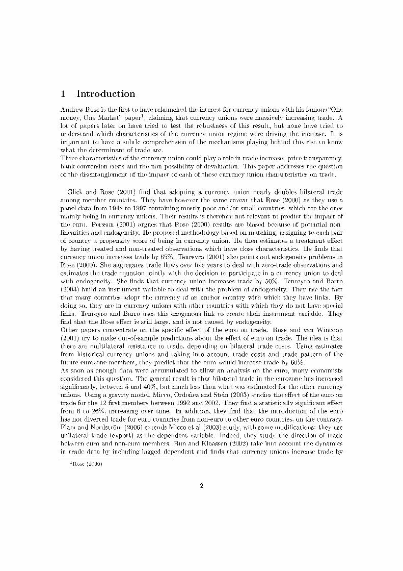
Disentangle the Eects on Trade:

Currency Union, Peg One-to-one and Simple Fixed

Exchange Rate

Laura Lebastard∗

June 24, 2016

Abstract

This paper compares the eects of currency unions, pegs one-to-one and classical xedexchange rates on bilateral trade. Indeed, peg one-to-one is a form of xed exchange ratebut with price transparency. Therefore my study can help to disentangle the eect of thexity of exchange rate and price transparency from the non-possibility of devaluation incurrency union observed eect of increasing trade. In order to do that, it uses the proximityof the peg one-to-one and the currency union to have a better understanding of the volumeof trade dierential.I study a two-country theoretical world economy with à la Melitz rms. I consider threecases: countries in currency union, in peg one-to-one or in simple xed exchange rate. I thenestimate the level of trade, rms taking into account cost of exporting (smaller for currencyunions) and probability of devaluation (rms being risk-averse).I use a panel data of 255 countries/regions from 1971 to 2014 and have constructed a databasefor three types of exchange rate regimes (currency unions, peg one-to-one and xed exchangerate). I nd that currency unions always have positive, signicant and higher eects ontrade than pegs one-to-one; and xed exchange rate has no signicant impact. However,peg one-to-one eect on trade turns to be endogenous. This reinforces the importance ofthe commitment dimension of the currency union in the impact on trade.

JEL Classication Numbers: F12, F13, F15, F31, F33, F41, F42

∗RITM, Univ. Paris-Sud, Université Paris-Saclay

1

1 Introduction

Andrew Rose is the rst to have relaunched the interest for currency unions with his famous Onemoney, One Market paper1, claiming that currency unions were massively increasing trade. Alot of papers later on have tried to test the robustness of this result, but none have tried tounderstand which characteristics of the currency union regime were driving the increase. It isimportant to have a subtle comprehension of the mechanisms playing behind this rise to knowwhat the determinant of trade are.Three characteristics of the currency union could play a role in trade increase: price transparency,bank conversion costs and the non-possibility of devaluation. This paper addresses the questionof the disentanglement of the impact of each of these currency union characteristics on trade.

Glick and Rose (2001) nd that adopting a currency union nearly doubles bilateral tradeamong member countries. They have however the same caveat that Rose (2000) as they use apanel data from 1948 to 1997 containing mostly poor and/or small countries, which are the onesmainly being in currency unions. Their results is therefore not relevant to predict the impact ofthe euro. Persson (2001) argues that Rose (2000) results are biased because of potential non-linearities and endogeneity. He proposed methodology based on matching, assigning to each pairof country a propensity score of being in currency union. He then estimates a treatment eectby having treated and non-treated observations which have close characteristics. He nds thatcurrency union increases trade by 65%. Tenreyro (2001) also points out endogeneity problems inRose (2000). She aggregates trade ows over ve years to deal with zero-trade observations andestimates the trade equation jointly with the decision to participate in a currency union to dealwith endogeneity. She nds that currency union increases trade by 50%. Tenreyro and Barro(2003) build an instrument variable to deal with the problem of endogeneity. They use the factthat many countries adopt the currency of an anchor country with which they have links. Bydoing so, they are in currency unions with other countries with which they do not have speciallinks. Tenreyro and Barro uses this exogenous link to create their instrument variable. Theynd that the Rose eect is still large, and is not caused by endogeneity.Other papers concentrate on the specic eect of the euro on trade. Rose and van Wincoop(2001) try to make out-of-sample predictions about the eect of euro on trade. The idea is thatthere are multilateral resistance to trade, depending on bilateral trade costs. Using estimatesfrom historical currency unions and taking into account trade costs and trade pattern of thefuture eurozone members, they predict that the euro would increase trade by 60%.As soon as enough data were accumulated to allow an analysis on the euro, many economistsconsidered this question. The general result is that bilateral trade in the eurozone has increasedsignicantly, between 5 and 40%, but much less than what was estimated for the other currencyunions. Using a gravity model, Micco, Ordoñez and Stein (2003) studies the eect of the euro ontrade for the 12 rst members between 1992 and 2002. They nd a statistically signicant eectfrom 6 to 26%, increasing over time. In addition, they nd that the introduction of the eurohas not diverted trade for euro countries from non-euro to other euro countries, on the contrary.Flam and Nordström (2006) extends Micco et al (2003) study, with some modications: they useunilateral trade (export) as the dependent variable. Indeed, they study the direction of tradebetween euro and non-euro members. Bun and Klaassen (2002) take into account the dynamicsin trade data by including lagged dependent and nds that currency unions increase trade by

1Rose (2000)

2

38% in the long run. Other evidence conrmed the nding: De Nardis and Vicarelli (2003),Barr, Breedon and Miles (2003), Berger and Nitsch (2005) and more recently Chintrakarn (2008)reported similar positive results.Glick and Rose (2015) test many methodologies to measure the eect of currency union on tradein the world and in the eurozone in order to compare them. They nd that the results are verysensitive to the econometric methodology, preventing to give a robust estimation. Nevertheless,they conclude that the eurozone has very small eect, if any. They nd the same range ofestimation than previous papers for the other currency unions.Finally, Frankel (2008) tries to explain the discrepancy between estimates of the euro's eect andestimates of the other currency unions. He tests the usual suspects: lag (euro being still young),size (euro countries being on average bigger) and endogeneity, but does not nd any evidencethat they explain such a big dierence. Instead, Frankel suspects the size of the sample to havean inuence.

The literature is much older and less prolic on the xed exchange rate side. The discussionis centered on the dierence of eect between xed and oating exchange rate and the questionremains open. There are mixed evidence on the subject. Most early articles2 estimated a largenegative correlation between nominal variability of exchange rate and trade while 1990's studies3

reported small and almost insignicant eects. The recent literature does not solve the problem.Nilsson and Nilsson (2000) study 6 regimes-types (not including currency unions) on a hundreddeveloping countries between 1983 and 1992 to measure the eect of exchange rate on export.They nd that the more exible the exchange rate, the greater the exports of developing countries.They give two reasons, specic to developing countries. First, there are severe consequences ofmisalignment of exchange rate as the exporters are more vulnerable due to their lack of marketpower (main exports being raw material and agricultural products). Second, exporters havelimited hedging possibilities. On the contrary, Fritz-Krockow and Jurzyk (2004) working on 24Caribbean and Latin America countries from 1960 to 2001 nd that the longer and more crediblethe peg, the higher the trade. However, they do not say how they measure the credibility ofthe peg. Tenreyro (2007) works on a 87 countries sample (developing and developed countries)between 1970 and 1997. To deal with the endogeneity and the measurement error of exchangerate variability, she develops an instrumental-variable version of the Poisson pseudo-maximumlikelihood (PPML) estimator (using the same IV than Tenreyro and Barro, 2003). The estimatesindicate that nominal exchange rate variability has no signicant impact on trade ows. Finally,Dorn and Egger (2013) uses 10 000 country-pairs from 1974 to 2004 and nd that countriespegged trade more, but only after about 8 years.With the arrival of Rose and the currency union literature, issues arose of the dierence in termof trade between currency union and xed exchange rate. Fritz-Krockow and Jurzyk (2004) ndthat peg has a signicant positive impact, but a currency union does not provides additionalbenets. On the contrary, Klein and Shambaugh (2004) studying 181 countries over the period1973-1999, estimate large and signicant eects of xed exchange rate on bilateral trade, andan eect even larger for currency unions. Fielding and Shields (2003) is the closest article tothis contribution to the best of my knowledge as it is the only one (even if it does not say it) tolook at the dierence between currency union and peg one-to-one by studying the CFA franc.However it only works on the CFA Franc sample and does not compare it to the rest of the world.Fielding and Shields nd that sharing a common currency is associated with substantially morebilateral trade, but only among the countries that are landlocked.

2Abrams (1980) and Thursby and Thursby (1987)3Frankel and Wei (1993), Eichengreen and Irwin (1996), and Frankel (1997)

3

The literature is largely proliferating concerning the link between currency union and tradeand between xed exchange rate and trade. However, to my knowledge, there is no specic studyabout the link between peg one-to-one and trade, peg one-to-one being the xed exchange rateregime the closest to currency union, as it allows price transparency (the conversion rate betweenthe currencies being equal to one). The exchange rate regime is so close to the currency unionthat some authors have pool them together4. For my study, I have built a database referencingall the pegs one-to-one since 1948.

Here could be a basic table of the dierent types of xed exchange rates, from the strongest,the currency union, to the weakest, classical xed exchange rate.

Exchangerate regim

No monetarypolicy power

Currencychange cost

Possibility ofdevaluation

Cost ofconversion

Dollarization/ euroisation XPeg One-to-one X X XFixed Exchange Rate X X X X

Table 1: Characteristics of several xed exchange rate regims compared with currency union,being the benchmark

In this paper, I take advantage of this panel of exchange rate regimes to disentangle the eectof each dierence on trade. First I build a theoretical model to explicit how the dierent charac-teristics of the exchange rate regimes (mainly trade cost and possibility of devaluation) inuencetrade. Then I estimate empirically how big the inuence of these characteristics is.

I nd that currency union increases trade more than peg one-to-one, both being positive andsignicant. I do not nd any eect from classical xed exchange rate. However it turns outpeg one-to-one eect is endogenous on my sample. On the short term, currency unions havevery strong eects, pegs one-to-one have small eects and classical xed exchange rates none.However on the long run, the eects of currency unions (that remain stable over time) and pegsone-to-one tend to converge. Classical xed exchange rate have small eects only after 15 years.

In section two, I present my model, disentangling the eects of each currency union charac-teristic on trade. In section three, I measure the eect of currency union, peg one-to-one andsimple xed exchange rate on trade empirically. Finally I conclude.

2 The Model

My model is related to Ghironi and Melitz (2005). I adopt their approach to compare tradein the dierent xed exchange rate regime: currency union, peg one-to-one and classical xedexchange rate. I use their model, and change rm's utility function by adding a disutility inprot volatility5 and by modulating the transport cost depending on the exchange rate regime

4Rose (2000)5In my case, the volatility comes from exchange rate variations. There are evidence rms seek ways to reduce

their exposure to exchange rate risk through domestic-currency invoicing and hedging. Devereux et al (2004) ndthat monetary stability increases the atractivity of a currency to be used as invoicing currency. Döhring (2008)

4

to make the model more realistic. I then see how my results dier from theirs.

2.1 Domestic market

I keep almost everything in the model of Ghironi and Melitz (2005) for the domestic market. Theworld consists of two symetric countries, denoted as the home country and the foreign country;foreign variables being denoted with a superscript star. Prices are exible and in nominal terms.Utility functions are similar at home and abroad and have a similar consumption basket.

2.1.1 Households

The economy consists of households and rms. The representative home household maximizes

expected intertemporal utility from consumption (C): Ut = Et

[∞∑s=t

βs−tC1−γs

1−γ

], 0 ≤ β ≤ 1 being

the subjective discount factor and γ > 0 the inverse of the intertemporal elasticity of substitution.Each rm produces a variety ω, which is an imperfect substitute to all other varieties over acontinum of goods Ω under conditions of monopolistic competition, θ > 1 being the symmetricelasticity of substituion across goods (I follow Ghironi and Melitz (2005) and take θ = 3.8 when

needed). Households consume the basket of goods Ct: Ct =

(∫ω∈Ω

ct(ω)θ−1θ dω

) θθ−1

. The

consumption-based price index at home is Pt =

(∫ω∈Ω

pt(ω)θ−1dω

) 1θ−1

, pt(ω) being the price

of a good ω. Finally, R denotes aggregate expenditure with Rt = PtCt =∫ω∈Ω

rt(ω)dω.

Therefore we have ct(ω) =

(pt(ω)Pt

)−θCt and rt(ω) =

(pt(ω)Pt

)1−θ

Rt.

2.1.2 Firms

Prior to entry, rms face an identical xed entry cost fE,t, paid on a period-by-period basis6.Production function is the following Ct = LZt − fE , production requiring only labor, and ag-gregate labor productivity being indexed by Zt. wt/Ztz is the cost per unit of the consumptiongood Ct, wt being the real wage and z the relative productivity, dierent for each rm. Let pD,tbeing the nominal domestic price of home rm, and ρD,t the real price:

ρD,t(z) ≡pD,t(z)

Pt=

θ

θ − 1

wtzZt

(1)

We therefore havect(z1)

ct(z2)=

(z1

z2

)θ(2)

rt(z1)

rt(z2)=

(z1

z2

)θ−1

(3)

nds that about 50% of euro-area exports to countries outside the EU are invoiced in euro, and this share is higherin exports to other EU countries. He also nds that Euro area non-nancial blue chip companies systematicallyuse nancial derivatives to hedge transaction risk.

6In the model of Ghironi and Melitz (2005), fE,t is only paid in the rst period

5

2.1.3 Prot and revenues for the rms

Domestic prot for home rms expressed in real terms in units of the consumption basket:

dD,t(z) =1

θ

[ρD,t(z)

]1−θCt − fE,t (4)

And domestic revenues (being equal to the sales at home) for home rms:

rD,t(z) =[ρD,t(z)

]1−θCt (5)

In every period, a mass ND,t of rms produces in the home country. These rms have a distri-bution of productivity level over [zmin,∞] given by G(z). Here is the average productivity levelfor all producing rm in each country:

zD ≡

[∫ ∞zD,min

zθ−1dG(z)

] 1θ−1

(6)

From (3), we can now calculate the domestic revenue of the average home rm

rD,t(zD) = rD,t =[ zDzD,min

]θ−1

rD,t(zD,min) (7)

Therefore the domestic prot of the average home rm is

dD,t =1

θ

[ zDzD,min

]θ−1

rD,t(zD,min)− fE,t (8)

The zero cuto prot condition, by pinning down the prot of the cuto rm implies

dD,t(zD,min) = 0⇐⇒ rD,t(zD,min) = θfE,t

therefore the domestic prot of the average rm is

dD,t =([ zDzD,min

]θ−1

− 1)fE,t (9)

and the domestic revenue of the average rm is

rD,t = θfE,t

[ zDzD,min

]θ−1

(10)

2.2 Foreign market

The rms have a disutility in prot volatility (relative to the initial value and not to the mean)due to the exchange rate, expressed in its export utility function. Prot made in domestic marketis therefore not aected by this disutility. Firms decide to enter on the foreign market beforeknowing the exchange rate. The rm sensitivity to volatility is captured by α ≥ 0:

UX,t(z) = Et(dX,t(z))− α√Vt(dX,t(z)) (11)

6

2.2.1 Price of exported goods

Only the most productive rms can export as exporting is costly, involving a melting-iceberg costτt ≥ 1 as well as a xed cost fX,t > fE,t (in real term wtfX,t/Zt) paid at each period. Let pX,tbe the general nominal export price of home rm, and ρX,t the real price, with Qt ≡ εtP

∗t /Pt

the consumption-based real exchange rate is:

ρX,t(z) ≡pX,t(z)

Pt= Q−1

t τtρD,t(z) (12)

The rm's utility function does not modied the price structure, which remains the same as inGhironi and Melitz (2005). Owing to ρD,t(z) shape (mark up being constant), the pass-throughis equal to one, increasing the importance of the exchange rate regime.Let the melting-iceberg cost be dierent if the rm exports to a country with the same currency,in peg one-to-one or in classical xed exchange rate. Indeed, as seen in table 1, the potentialcosts are not the same. Let 1 ≤ τ1,t < τ2,t < τ3,t, τ1 being the transport cost, τ2 the bank feeson foreign currency change and τ3 the conversion cost.Price for currency union:

ρcu,X,t(z) ≡pcu,X,t(z)

Pt=PtP ∗t

τ1,tρD,t(z)

Price for peg one-to-one:

ρpeg,X,t(z) ≡ppeg,X,t(z)

Pt=(P ∗tPt

D)−1

τ1,tτ2,tρD,t(z)

Price for classical xed exchange rate:

ρfix,X,t(z) ≡pfix,X,t(z)

Pt=(εP ∗tPt

D)−1

τ1,tτ2,tτ3,tρD,t(z)

with D = 1 (no devaluation) with probability Pt and D = η 6= 1 (η > 0 being the change,appreciation or depreciation, in the exchange rate from the initial state) with probability 1−Pt.The probability Pt of no devaluation depends on the credibility φ of the exchange rate regime,and its history (has the peg held for a long time already).Currency union : Pt(φCU ) = 1Peg one-to-one : Pt(φpeg) = Pt(φpeg(φpeg,t−1)) < Pt(φCU )Fixed exchange rate : Pt(φfix) = Pt(φfix(φfix,t−1)) < Pt(φpeg)In the long run, if there has been no devaluation, Pt(φpeg) and Pt(φfix) tend towards 1 with thecredibility increase. Therefore, the dierence in trade will only be caused by τ2,t and τ3,t. It istherefore possible to disentangle the two eects empirically.

The cost of exporting depends on the exchange rate regime. As only rms with a big enoughmarkup can export, there will be now 4 dierent types of rms: those not exporting, thoseexporting only in the currency union, those exporting in the currency union and with countriesbeing in peg one-to-one, and those exporting everywhere. In the model of Ghironi and Melitz,there is no such types.

2.2.2 Prots and revenues from sales abroad

The total prot of a home rm will be the sum of its prot at home and abroad: dt(z) =dD,t(z) + dX,t(z) with dX,t(z) being:

dX,t(z) =Qtθ

[ρX,t(z)

]1−θC∗t −

wtfX,tZt

(13)

7

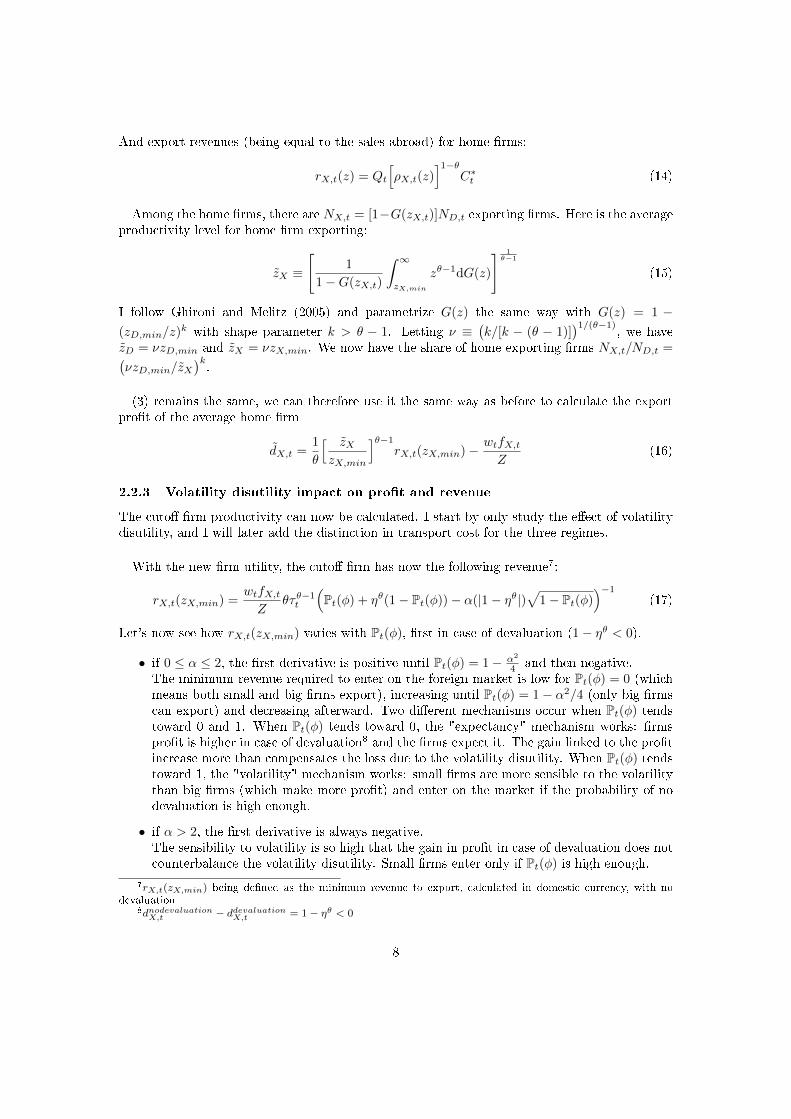
And export revenues (being equal to the sales abroad) for home rms:

rX,t(z) = Qt

[ρX,t(z)

]1−θC∗t (14)

Among the home rms, there are NX,t = [1−G(zX,t)]ND,t exporting rms. Here is the averageproductivity level for home rm exporting:

zX ≡

[1

1−G(zX,t)

∫ ∞zX,min

zθ−1dG(z)

] 1θ−1

(15)

I follow Ghironi and Melitz (2005) and parametrize G(z) the same way with G(z) = 1 −(zD,min/z)

k with shape parameter k > θ − 1. Letting ν ≡(k/[k − (θ − 1)]

)1/(θ−1), we have

zD = νzD,min and zX = νzX,min. We now have the share of home exporting rms NX,t/ND,t =(νzD,min/zX

)k.

(3) remains the same, we can therefore use it the same way as before to calculate the exportprot of the average home rm

dX,t =1

θ

[ zXzX,min

]θ−1

rX,t(zX,min)− wtfX,tZ

(16)

2.2.3 Volatility disutility impact on prot and revenue

The cuto rm productivity can now be calculated. I start by only study the eect of volatilitydisutility, and I will later add the distinction in transport cost for the three regimes.

With the new rm utility, the cuto rm has now the following revenue7:

rX,t(zX,min) =wtfX,tZ

θτθ−1t

(Pt(φ) + ηθ(1− Pt(φ))− α(|1− ηθ|)

√1− Pt(φ)

)−1

(17)

Let's now see how rX,t(zX,min) varies with Pt(φ), rst in case of devaluation (1− ηθ < 0).

• if 0 ≤ α ≤ 2, the rst derivative is positive until Pt(φ) = 1− α2

4 and then negative.The minimum revenue required to enter on the foreign market is low for Pt(φ) = 0 (whichmeans both small and big rms export), increasing until Pt(φ) = 1− α2/4 (only big rmscan export) and decreasing afterward. Two dierent mechanisms occur when Pt(φ) tendstoward 0 and 1. When Pt(φ) tends toward 0, the "expectancy" mechanism works: rmsprot is higher in case of devaluation8 and the rms expect it. The gain linked to the protincrease more than compensates the loss due to the volatility disutility. When Pt(φ) tendstoward 1, the "volatility" mechanism works: small rms are more sensible to the volatilitythan big rms (which make more prot) and enter on the market if the probability of nodevaluation is high enough.

• if α > 2, the rst derivative is always negative.The sensibility to volatility is so high that the gain in prot in case of devaluation does notcounterbalance the volatility disutility. Small rms enter only if Pt(φ) is high enough.

7rX,t(zX,min) being dened as the minimum revenue to export, calculated in domestic currency, with nodevaluation

8dnodevaluationX,t − ddevaluationX,t = 1− ηθ < 0

8

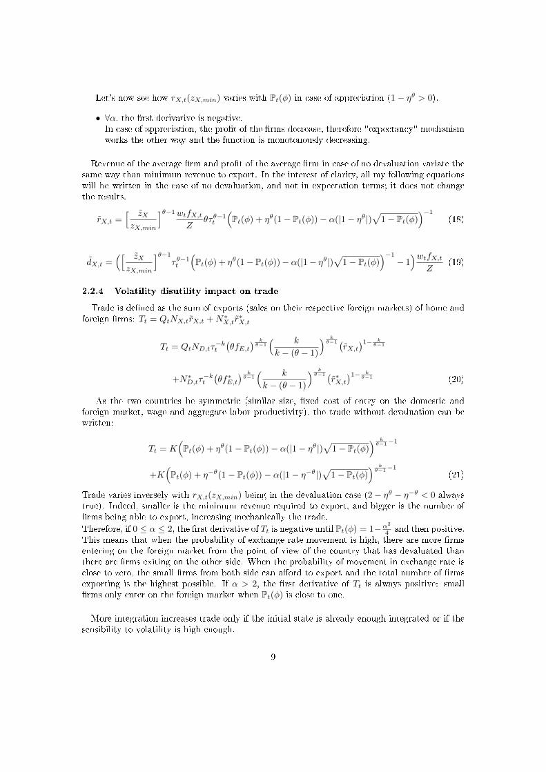
Let's now see how rX,t(zX,min) varies with Pt(φ) in case of appreciation (1− ηθ > 0).

• ∀α, the rst derivative is negative.In case of appreciation, the prot of the rms decrease, therefore "expectancy" mechanismworks the other way and the function is monotonously decreasing.

Revenue of the average rm and prot of the average rm in case of no devaluation variate thesame way than minimum revenue to export. In the interest of clarity, all my following equationswill be written in the case of no devaluation, and not in expectation terms; it does not changethe results.

rX,t =[ zXzX,min

]θ−1wtfX,tZ

θτθ−1t

(Pt(φ) + ηθ(1− Pt(φ))− α(|1− ηθ|)

√1− Pt(φ)

)−1

(18)

dX,t =([ zXzX,min

]θ−1

τθ−1t

(Pt(φ) + ηθ(1− Pt(φ))− α(|1− ηθ|)

√1− Pt(φ)

)−1

− 1)wtfX,t

Z(19)

2.2.4 Volatility disutility impact on trade

Trade is dened as the sum of exports (sales on their respective foreign markets) of home andforeign rms: Tt = QtNX,trX,t +N∗X,tr

∗X,t

Tt = QtND,tτ−kt

(θfE,t

) kθ−1

( k

k − (θ − 1)

) kθ−1 (

rX,t)1− k

θ−1

+N∗D,tτ−kt

(θf∗E,t

) kθ−1

( k

k − (θ − 1)

) kθ−1 (

r∗X,t)1− k

θ−1 (20)

As the two countries be symmetric (similar size, xed cost of entry on the domestic andforeign market, wage and aggregate labor productivity), the trade without devaluation can bewritten:

Tt = K(Pt(φ) + ηθ(1− Pt(φ))− α(|1− ηθ|)

√1− Pt(φ)

) kθ−1−1

+K(Pt(φ) + η−θ(1− Pt(φ))− α(|1− η−θ|)

√1− Pt(φ)

) kθ−1−1

(21)

Trade varies inversely with rX,t(zX,min) being in the devaluation case (2− ηθ − η−θ < 0 alwaystrue). Indeed, smaller is the minimum revenue required to export, and bigger is the number ofrms being able to export, increasing mechanically the trade.

Therefore, if 0 ≤ α ≤ 2, the rst derivative of Tt is negative until Pt(φ) = 1−α2

4 and then positive.This means that when the probability of exchange rate movement is high, there are more rmsentering on the foreign market from the point of view of the country that has devaluated thanthere are rms exiting on the other side. When the probability of movement in exchange rate isclose to zero, the small rms from both side can aord to export and the total number of rmsexporting is the highest possible. If α > 2, the rst derivative of Tt is always positive: smallrms only enter on the foreign market when Pt(φ) is close to one.

More integration increases trade only if the initial state is already enough integrated or if thesensibility to volatility is high enough.

9

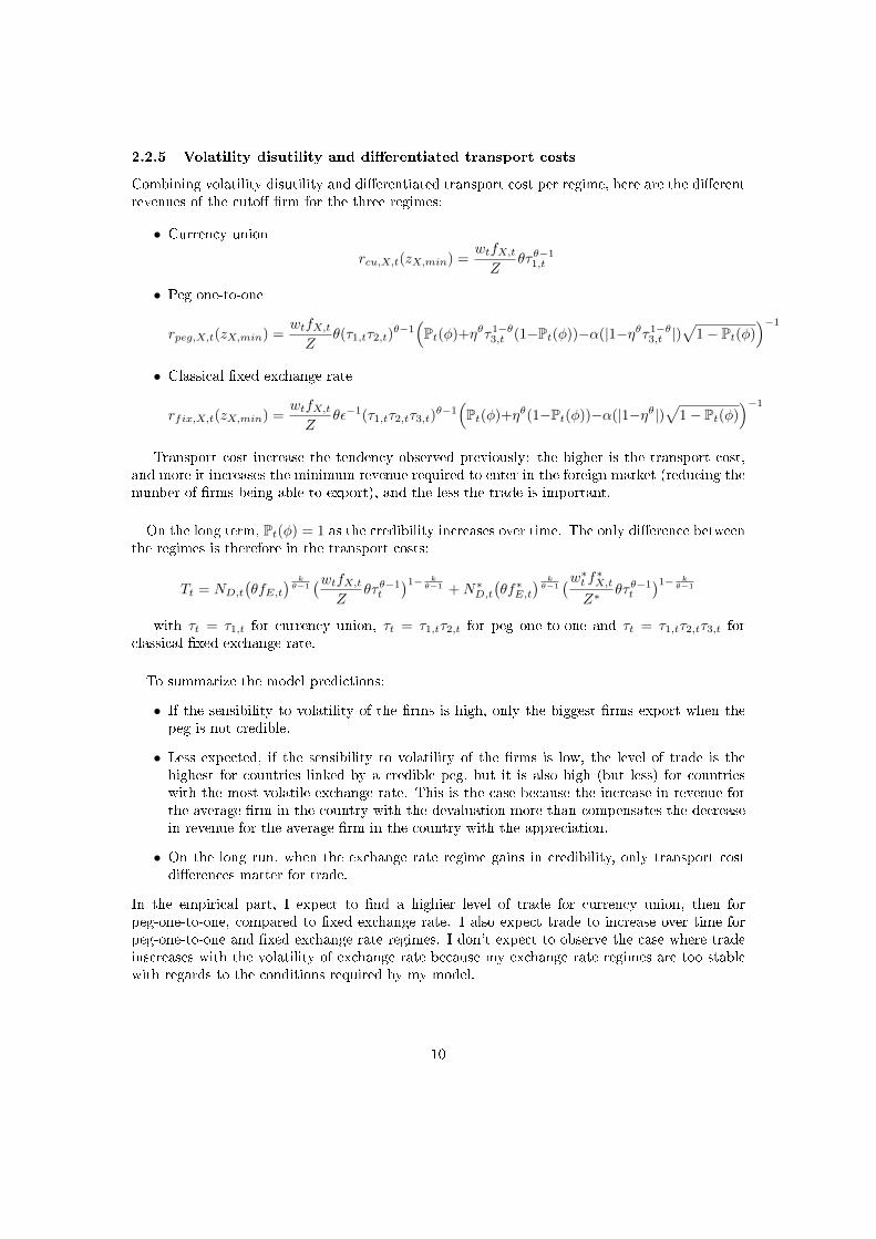
2.2.5 Volatility disutility and dierentiated transport costs

Combining volatility disutility and dierentiated transport cost per regime, here are the dierentrevenues of the cuto rm for the three regimes:

• Currency union

rcu,X,t(zX,min) =wtfX,tZ

θτθ−11,t

• Peg one-to-one

rpeg,X,t(zX,min) =wtfX,tZ

θ(τ1,tτ2,t)θ−1(Pt(φ)+ηθτ1−θ

3,t (1−Pt(φ))−α(|1−ηθτ1−θ3,t |)

√1− Pt(φ)

)−1

• Classical xed exchange rate

rfix,X,t(zX,min) =wtfX,tZ

θε−1(τ1,tτ2,tτ3,t)θ−1(Pt(φ)+ηθ(1−Pt(φ))−α(|1−ηθ|)

√1− Pt(φ)

)−1

Transport cost increase the tendency observed previously: the higher is the transport cost,and more it increases the minimum revenue required to enter in the foreign market (reducing thenumber of rms being able to export), and the less the trade is important.

On the long term, Pt(φ) = 1 as the credibility increases over time. The only dierence betweenthe regimes is therefore in the transport costs:

Tt = ND,t(θfE,t

) kθ−1(wtfX,t

Zθτθ−1t

)1− kθ−1 +N∗D,t

(θf∗E,t

) kθ−1(w∗t f∗X,t

Z∗θτθ−1t

)1− kθ−1

with τt = τ1,t for currency union, τt = τ1,tτ2,t for peg one-to-one and τt = τ1,tτ2,tτ3,t forclassical xed exchange rate.

To summarize the model predictions:

• If the sensibility to volatility of the rms is high, only the biggest rms export when thepeg is not credible.

• Less expected, if the sensibility to volatility of the rms is low, the level of trade is thehighest for countries linked by a credible peg, but it is also high (but less) for countrieswith the most volatile exchange rate. This is the case because the increase in revenue forthe average rm in the country with the devaluation more than compensates the decreasein revenue for the average rm in the country with the appreciation.

• On the long run, when the exchange rate regime gains in credibility, only transport costdierences matter for trade.

In the empirical part, I expect to nd a highier level of trade for currency union, then forpeg-one-to-one, compared to xed exchange rate. I also expect trade to increase over time forpeg-one-to-one and xed exchange rate regimes. I don't expect to observe the case where tradeinscreases with the volatility of exchange rate because my exchange rate regimes are too stablewith regards to the conditions required by my model.

10

3 Empirical results

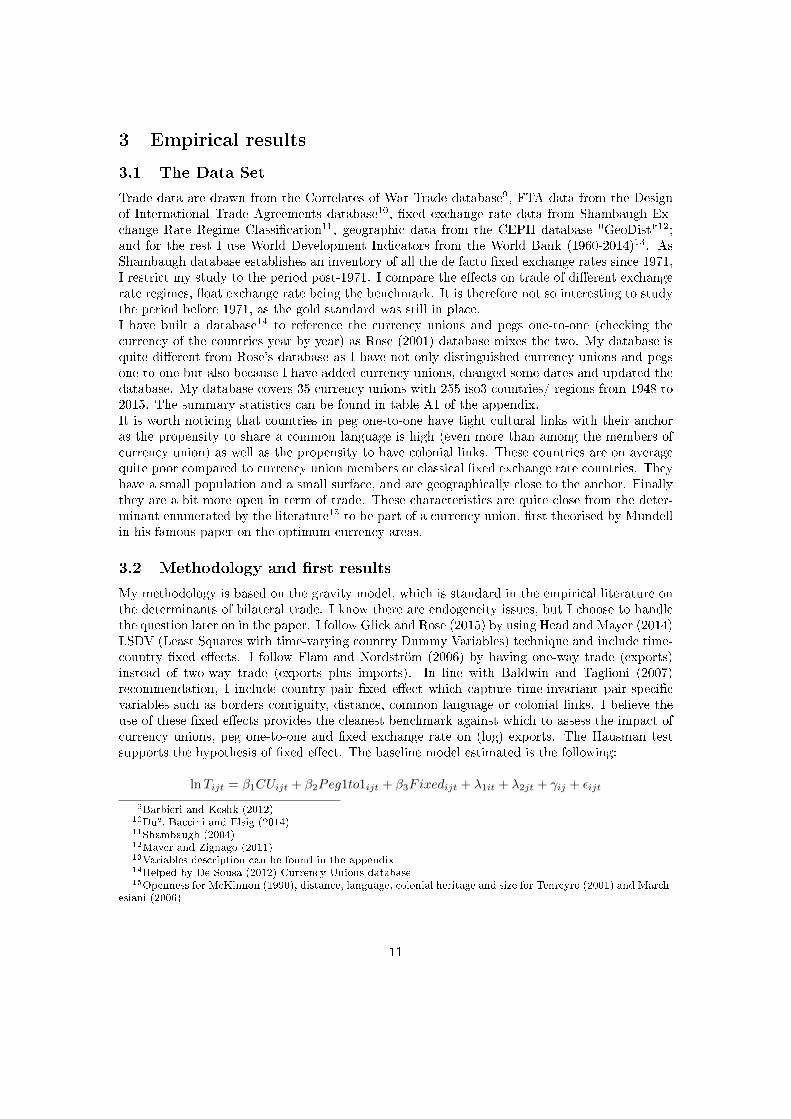
3.1 The Data Set

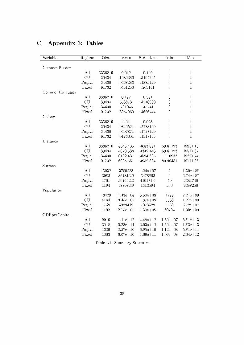
Trade data are drawn from the Correlates of War Trade database9, FTA data from the Designof International Trade Agreements database10, xed exchange rate data from Shambaugh Ex-change Rate Regime Classication11, geographic data from the CEPII database "GeoDist"12;and for the rest I use World Development Indicators from the World Bank (1960-2014)13. AsShambaugh database establishes an inventory of all the de facto xed exchange rates since 1971,I restrict my study to the period post-1971. I compare the eects on trade of dierent exchangerate regimes, oat exchange rate being the benchmark. It is therefore not so interesting to studythe period before 1971, as the gold standard was still in place.I have built a database14 to reference the currency unions and pegs one-to-one (checking thecurrency of the countries year by year) as Rose (2001) database mixes the two. My database isquite dierent from Rose's database as I have not only distinguished currency unions and pegsone-to-one but also because I have added currency unions, changed some dates and updated thedatabase. My database covers 35 currency unions with 255 iso3 countries/ regions from 1948 to2015. The summary statistics can be found in table A1 of the appendix.It is worth noticing that countries in peg one-to-one have tight cultural links with their anchoras the propensity to share a common language is high (even more than among the members ofcurrency union) as well as the propensity to have colonial links. These countries are on averagequite poor compared to currency union members or classical xed exchange rate countries. Theyhave a small population and a small surface, and are geographically close to the anchor. Finallythey are a bit more open in term of trade. These characteristics are quite close from the deter-minant enumerated by the literature15 to be part of a currency union, rst theorised by Mundellin his famous paper on the optimum currency areas.

3.2 Methodology and rst results

My methodology is based on the gravity model, which is standard in the empirical literature onthe determinants of bilateral trade. I know there are endogeneity issues, but I choose to handlethe question later on in the paper. I follow Glick and Rose (2015) by using Head and Mayer (2014)LSDV (Least Squares with time-varying country Dummy Variables) technique and include time-country xed eects. I follow Flam and Nordström (2006) by having one-way trade (exports)instead of two-way trade (exports plus imports). In line with Baldwin and Taglioni (2007)recommendation, I include country-pair xed eect which capture time-invariant pair-specicvariables such as borders contiguity, distance, common language or colonial links. I believe theuse of these xed eects provides the cleanest benchmark against which to assess the impact ofcurrency unions, peg one-to-one and xed exchange rate on (log) exports. The Hausman testsupports the hypothesis of xed eect. The baseline model estimated is the following:

lnTijt = β1CUijt + β2Peg1to1ijt + β3Fixedijt + λ1it + λ2jt + γij + εijt

9Barbieri and Keshk (2012)10Dur, Baccini and Elsig (2014)11Shambaugh (2004)12Mayer and Zignago (2011)13Variables description can be found in the appendix14Helped by De Sousa (2012) Currency Unions database15Openness for McKinnon (1990), distance, language, colonial heritage and size for Tenreyro (2001) and March-

esiani (2006)

11

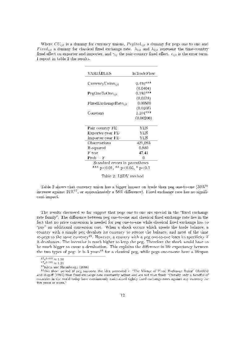
Where CUijt is a dummy for currency unions, Peg1to1ijt a dummy for pegs one-to-one andFixedijt a dummy for classical xed exchange rate. λ1it and λ2jt represent the time-countryxed eect on exporter and importer, and γij the pair-country xed eect. εijt is the error term.I report in table 2 the results.

VARIABLES lnTradeFlow

CurrencyUnionijt 0.410***(0.0404)

PegOneToOneijt 0.195***(0.0578)

FixedExchangeRateijt -0.00580(0.0108)

Constant 1.104***(0.00206)

Pair-country FE YESExporter-year FE YESImporter-year FE YESObservations 421,083R-squared 0.880F-test 47.41Prob > F 0

Standard errors in parentheses*** p<0.01, ** p<0.05, * p<0.1

Table 2: LSDV method

Table 2 shows that currency union has a bigger impact on trade than peg one-to-one (50%16

increase against 21%17, or approximately a 58% dierence). Fixed exchange rate has no signi-cant impact.

The results discussed so far suggest that pegs one-to-one are special in the xed exchangerate family. The dierence between peg one-to-one and classical xed exchange rate lies in thefact that no price conversion is needed for peg one-to-one while classical xed exchange has topay an additional conversion cost. When a shock occurs which upsets the trade balance, acountry with a simple peg devalues its currency to restore the balance, and most of the timere-pegs to the same currency18. However, a country with a peg one-to-one loses its specicity ifit devaluates. The incentive is much higher to keep the peg. Therefore the shock would have tobe much bigger to cause a devaluation. This explains the dierence in life expectancy betweenthe two types of peg: it is 3 years19 for a classical peg, while pegs one-to-one have a lifespan

16e0.410 ≈ 1.5017e0.195 ≈ 1.2118Klein and Shambaugh (2008)19this short period of peg supports the idea presented in The Mirage of Fixed Exchange Rates Obstfeld

and Rogo (1995) that xed exchange rate constantly adjust and are not that xed: literally only a handful ofcountries in the world today have continuously maintained tightly xed exchange rates against any currency forve years or more.

12

of 16 years. This gap potentially implies fundamental dierences between them. Knowing this,investors and traders act dierently and it has an impact on the economic activity.

I then use a dierent empirical model to check robustness by estimating a traditional gravityequation, without pair-country and time-country xed eect. I reproduce the results of Barroand Tenreyro (2007) and add a peg one-to-one dummy and a xed exchange rate dummy. Table3 presents these results.

13

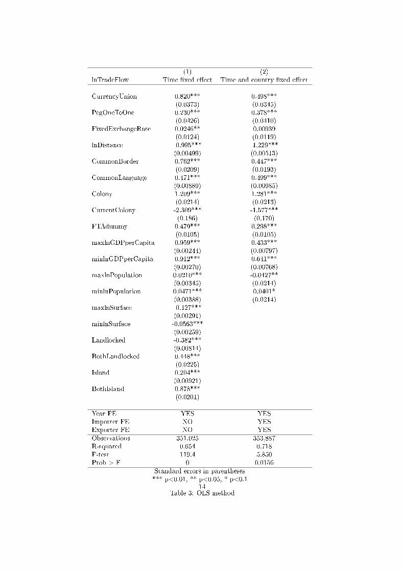
(1) (2)lnTradeFlow Time xed eect Time and country xed eect

CurrencyUnion 0.820*** 0.498***(0.0373) (0.0345)

PegOneToOne 0.230*** 0.378***(0.0426) (0.0410)

FixedExchangeRate 0.0246** 0.00939(0.0124) (0.0119)

lnDistance -0.995*** -1.229***(0.00499) (0.00513)

CommonBorder 0.762*** 0.447***(0.0209) (0.0193)

CommonLanguage 0.471*** 0.499***(0.00889) (0.00985)

Colony 1.209*** 1.281***(0.0214) (0.0213)

CurrentColony -2.309*** -1.577***(0.186) (0.170)

FTAdummy 0.479*** 0.298***(0.0105) (0.0105)

maxlnGDPperCapita 0.959*** 0.433***(0.00244) (0.00797)

minlnGDPperCapita 0.912*** 0.641***(0.00270) (0.00768)

maxlnPopulation 0.0210*** -0.0427**(0.00345) (0.0214)

minlnPopulation 0.0471*** 0.0401*(0.00388) (0.0214)

maxlnSurface -0.127***(0.00291)

minlnSurface -0.0563***(0.00259)

Landlocked -0.382***(0.00814)

BothLandlocked 0.448***(0.0225)

Island 0.204***(0.00921)

BothIsland 0.878***(0.0201)

Year FE YES YESImporter FE NO YESExporter FE NO YESObservations 351,025 353,887R-squared 0.654 0.718F-test 119.4 5.850Prob > F 0 0.0156


Table 3: OLS method14

This exercise suggests that currency unions increase trade by 127%20 against 26%20 for pegwith time xed eect, and by 65%20 against 46%20 with both time and country xed eect.Fixed exchange rate eect on trade is very small in the rst case (2.4%20) and insignicantin the second. The rst thing that jumps out from this comparison with table 2 is that myresults are quite dierent from one specication to the next. This discrepancy is pointed out byGlick and Rose (2015): estimates of the currency union eect on trade are sensitive to the exacteconometric methodology. Therefore, I only focus on the relative dierence between currencyunions and pegs one-to-one and not on the levels, as they uctuate so much. Nevertheless, myndings for currency union are in the range of the ones found in the literature21. They arehowever higher than the ones only measuring the eect of the euro on bilateral trade22. Glickand Rose (2015) also nd much bigger eects if they take the world in their sample rather thanonly the eurozone23.

The story that emerges from both tables is that currency union still has a bigger impact ontrade than peg one-to-one. Table 3 shows biggest dierences of eect between currency unionand peg one-to-one than LSDV methodology (table 2), around an 80% dierence with onlytime xed-eect, and a 30% dierence adding country-xed eect. The coecient of the xedexchange rate dummies is not signicant, which means that a classical xed exchange rate doesnot aect bilateral trade. My ndings are in line with Tenreyro (2006).

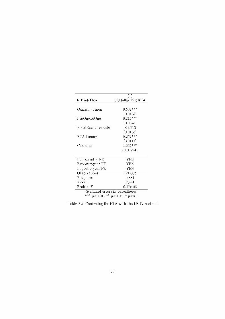
I control for trade increase from free trade agreements by including to the LSDV regression aFTA dummy24, following Micco, Stein and Ordoñez (2003) as it can inuence bilateral trade. Ithas almost no inuence.

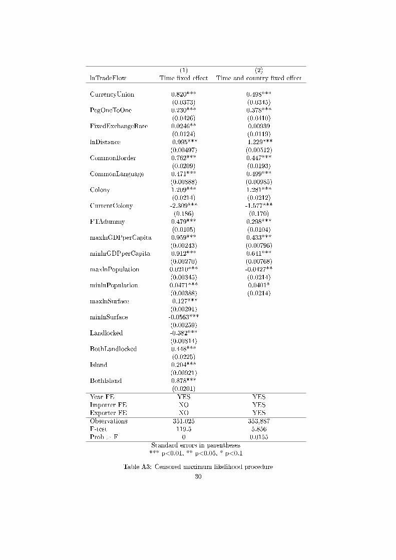
One problem with the logarithm of export is that it leads to the exclusion of observationswith zeros values. In order to address this potential bias, I follow Barro and Tenreyro (2007)and estimate the gravity equation with a censored maximum likelihood procedure. The results(table A3 in the appendix) are close to those obtained above and do not reverse the trend ofcurrency union having a bigger eect than peg one-to-one. This suggests that my coecients arenot aected by the exclusion of the zero-valued observations.

Short run versus long run Klein and Shambaugh (2004) have established that the expectedduration of a peg increases dramatically if it survives two years. Klein and Shambaugh (2008)have calculated that the probability of having a xed exchange rate given it was xed the previousyear is 82%; and this conditional survival rate increases with the number of years already spentin the spell. Fritz-Krockow and Jurzyk (2004) have established that longer was a peg and morepositive was its impact on bilateral trade. According to Dorn and Egger (2013), the eect issignicant after 8 years.I investigate whether my estimations are sensitive to the duration of the exchange rate regimeby comparing short term and long term specications. Table 4 presents the dierent estimationsfor currency unions/pegs one-to-one younger than 5 years, between 5 and 10 years, etcetera untilmore than 20 years.

20e0.820 ≈ 2.27; e0.230 ≈ 1.26; e0.498 ≈ 1.65; e0.378 ≈ 1.46; e0.0246 ≈ 1.02421Persson (2001) nds 61% and Tenreyro (2001) 50%22Micco, Ordoñez and Stein (2003) nds between 6 and 26%; Bun and Klaassen (2002) nds 38%; Flam and

Nordström (2006) 15%23Frankel (2008) tries to explain this discrepancy but fail to charge the three usual suspects: lack of hindsight

as euro is still young, dierence of size as euro members are on average bigger, and endogeneity problems.24The results are displayed in table A2 in the appendix

15

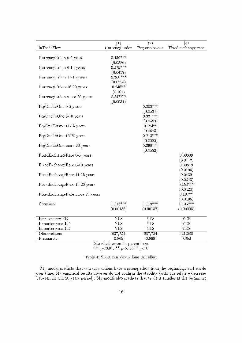
(1) (2) (3)lnTradeFlow Currency union Peg one-to-one Fixed exchange rate

CurrencyUnion 0-5 years 0.459***(0.0386)



CurrencyUnion 16-20 years 0.246**(0.101)

CurrencyUnion more 20 years 0.547***(0.0934)

PegOneToOne 0-5 years 0.303***(0.0521)


PegOneToOne 11-15 years 0.124**(0.0625)


PegOneToOne more 20 years 0.399***(0.0582)

FixedExchangeRate 0-5 years 0.00309(0.0112)



FixedExchangeRate 16-20 years 0.158***(0.0420)

FixedExchangeRate more 20 years 0.107**(0.0496)

Constant 1.117*** 1.119*** 1.106***(0.00155) (0.00152) (0.00205)

Pair-country FE YES YES YESExporter-year FE YES YES YESImporter-year FE YES YES YESObservations 637,754 637,754 421,083R-squared 0.869 0.869 0.880


Table 4: Short run versus long run eect

My model predicts that currency unions have a strong eect from the beginning, and stableover time. My empirical results however do not conrm the stability (with the relative decreasebetween 11 and 20 years period). My model also predicts that trade is smaller at the beginning

16

for peg one-to-one and xed exchange rate compared to currency union, and increases overtime linearly. However for the peg one-to-one as for the currency union, the empirical resultsshows a non linearity between 11 and 20 years period. The curve shape can be explained by twocontradictory mechanism: on one side, the credibility of the regime increases and therefore, tradeshould increase. On the other side, De Sousa (2012) shows that the eect of currency union ontrade is decreasing over time, and it could be the same for peg one-to-one.After 20 years, the dierence is quite small between currency union and peg one-to-one as pegone-to-one has gained credibility. Therefore, the dierence between the gap in the 0-5 yearperiod, and the gap in the +20 year period represents the gain of commitment/credibility. At aninnite horizon, the gap between currency union and peg one-to-one would represent the cost ofchange between currencies (embodied by τ2,t in my model), as there would be no more dierencein credibility between currency union and peg one-to-one. Classical xed exchange rate eect ontrade is not signicant in the short run, and becomes signicant after 15 years even though it isnot very high (around 17%25). This is in range with what my model predicts.

3.3 Problems of endogeneity

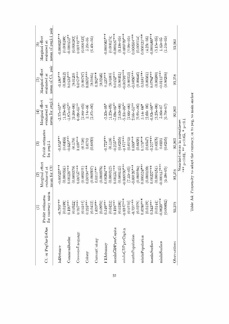
There is one additional issue that I need to address in order to get a more reliable view on theeect of these dierent exchange rate regimes on trade. These regressions suer from problemsof endogeneity: countries, because they trade a lot, decide to have a currency union or a pegone-to-one. The potential endogeneity is not necessarily captured by the xed eect. One wayto capture it is to use an instrumental variable. I use the instrument developed by Barro andTenreyro (2007). The main idea is that a country A has a certain probability to get into acurrency union with another country B. This probability depends on many factors, like distance,colonial links, common language, etc. Country C will also have a certain probability to getinto a currency union with country B. The fact that country A and C are in a currency unionis therefore exogenous as the factors leading to this decision are not transitive (for examplegeographical distance, or languages if a country has more than one).Frankel (2008) uses this exogenous event in a case study to show the eect on trade. Some Frenchcolonies were pegged to France and France joined the eurozone which creates an exogenous pegbetween the rest of the eurozone and these former colonies. Frankel showed that trade increasedby 76% between them, proving causality.I follow the same methodology as Barro and Tenreyro (2007) and estimate the probability thata given country gets into a currency union with one of the main six countries (Australia, France,Germany, Japan, the UK and the USA)26 using a probit, that can be found in table A4 in theappendix. The IV is obtained by computing the joint probability that two independent countriesenter in the same currency union (table 5).

25e0.158 ≈ 1.1726extended to India, South Africa, Belgium, Portugal, Spain, Russia, and New Zealand but the estimations do

not change signicantly

17

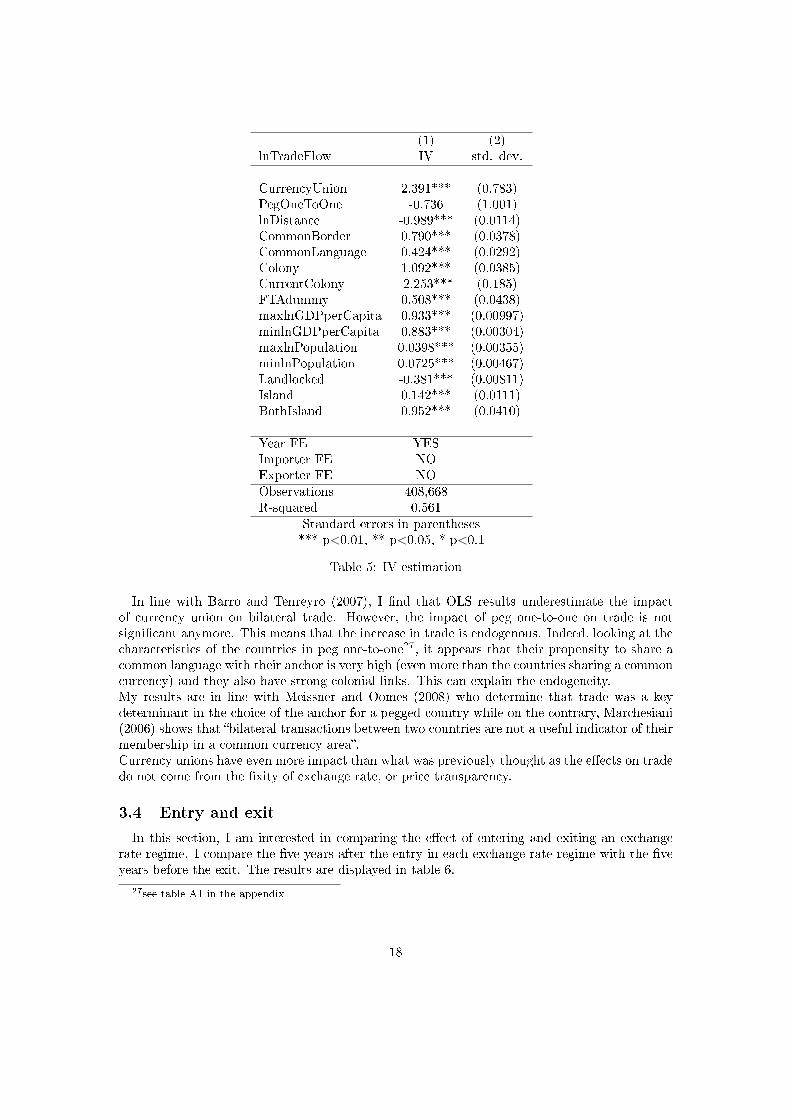
(1) (2)lnTradeFlow IV std. dev.

CurrencyUnion 2.391*** (0.783)PegOneToOne -0.736 (1.001)lnDistance -0.989*** (0.0114)CommonBorder 0.790*** (0.0378)CommonLanguage 0.424*** (0.0292)Colony 1.092*** (0.0385)CurrentColony -2.253*** (0.185)FTAdummy 0.508*** (0.0438)maxlnGDPperCapita 0.933*** (0.00997)minlnGDPperCapita 0.883*** (0.00304)maxlnPopulation 0.0398*** (0.00355)minlnPopulation 0.0725*** (0.00467)Landlocked -0.381*** (0.00811)Island 0.142*** (0.0111)BothIsland 0.952*** (0.0410)

Year FE YESImporter FE NOExporter FE NOObservations 408,668R-squared 0.561


Table 5: IV estimation

In line with Barro and Tenreyro (2007), I nd that OLS results underestimate the impactof currency union on bilateral trade. However, the impact of peg one-to-one on trade is notsignicant anymore. This means that the increase in trade is endogenous. Indeed, looking at thecharacteristics of the countries in peg one-to-one27, it appears that their propensity to share acommon language with their anchor is very high (even more than the countries sharing a commoncurrency) and they also have strong colonial links. This can explain the endogeneity.My results are in line with Meissner and Oomes (2008) who determine that trade was a keydeterminant in the choice of the anchor for a pegged country while on the contrary, Marchesiani(2006) shows that bilateral transactions between two countries are not a useful indicator of theirmembership in a common currency area.Currency unions have even more impact than what was previously thought as the eects on tradedo not come from the xity of exchange rate, or price transparency.

3.4 Entry and exit

In this section, I am interested in comparing the eect of entering and exiting an exchangerate regime. I compare the ve years after the entry in each exchange rate regime with the veyears before the exit. The results are displayed in table 6.

27see table A1 in the appendix

18

(1)VARIABLES lnTradeFlow

entryCurrencyUnion 0.336***(0.0387)

exitCurrencyUnion 0.630***(0.0794)

entryPegOneToOne 0.132**(0.0637)

exitPegOneToOne 0.221***(0.0423)

entryFixedExchangeRate 0.0146(0.0130)

exitFixedExchangeRate -0.0507***(0.0143)

Pair-country FE YESExporter-year FE YESImporter-year FE YESObservations 635,952R-squared 0.868


Table 6: Entry and exit

The eect on trade is always bigger for currency unions than for the other exchange rateregimes, whether we compare entries, or exits. The eect is bigger at the exit both in the case ofcurrency union and peg one-to-one. Maybe it is linked to the fact that, as we have seen in table4, the eect on trade tends to increase over time.

I then try to study specically the eect of switching from an exchange rate regime to another.I work on a twenty-year period: ten years before and after a switch. Table 7 presents the resultsfor entries: in column 1, among the switch to a oat regime, what was the eect on trade of beingpreviously in either currency union, peg one-to-one, or xed exchange rate. Table 8 presents theresults for exits.

The eect of entering or exiting from a currency union (line 1 of table 7 and 8) is alwaysbig and signicant except when leaving or entering a peg one-to-one. It would therefore meanthat the exchange rate regimes are quite close. On the contrary, column 2 of table 7 and 8 isnever signicant, as the eect of peg one-to-one, xed exchange rate and oat are compared tocurrency union.

19

(1) (2) (3) (4)lnTradeFlow to Float to CU to Peg to Fixed

SwitchingFromCurrencyUnion 0.273** 0.493 3.270***(0.109) (1.134) (1.219)

SwitchingFromPegOneToOne 0.208** 0.0425 -0.364(0.0927) (54,374) (0.270)

SwitchingFromFixedExchangeRate -0.0836*** 0.00646 3.554(0.0236) (0.120) (2.213)

SwitchingFromFloatExchangeRate 0.0927 -2.765 0.0138(0.0941) (158,016) (0.0266)

Pair-country FE YES YES YES YESExporter-year FE YES YES YES YESImporter-year FE YES YES YES YESObservations 90,663 4,468 1,154 73,058R-squared 0.906 0.991 0.989 0.910F-test 9.426 0.240 1.296 3.916Prob > F 8.06e-05 0.786 0.274 0.0199


Table 7: Entry

(1) (2) (3) (4)lnTradeFlow from Float from CU from Peg from Fixed

SwitchingToCurrencyUnion 0.324*** -14.72 0.365***(0.105) (12,008) (0.0797)

SwitchingToPegOneToOne -0.119 -0.0307 0.163(0.211) (0.371) (0.370)

SwitchingToFixedExchangeRate -0.00824 -0.146 -0.320*(0.0260) (0.476) (0.164)

SwitchingToFloatExchangeRate -0.0518 -0.411*** 0.0836***(0.361) (0.133) (0.0237)

Pair-country FE YES YES YES YESExporter-year FE YES YES YES YESImporter-year FE YES YES YES YESObservations 75,375 2,431 5,649 86,220R-squared 0.913 0.970 0.967 0.910F-test 5.305 0.0454 1.42e-06 6.184Prob > F 0.00497 0.956 0.999 0.00206


Table 8: Exit

20

4 Conclusion

In conclusion, there is denitely something special about peg one-to-one, it has neither thecharacteristics of the currency union, nor the ones of classical exchange rate. Indeed, its positiveimpacts on trade increase over time and tend in the long run to be close to the currency unioneects; however they turn out to be endogenous, contrary to the currency union's. Peg one-to-one should therefore be moved aside from the studies on currency unions and be studied on itsown, especially in order to understand the reason of its longevity.

My study conrms the important and positive eects of currency union on trade and showsit does not come from the xity of exchange rate or price transparency, but from credibility.Indeed, a common currency is seen as a much more serious and durable commitment thanother monetary arrangements (McCallum, 1995), the currency union regime credibility is evenmore important than what researchers thought: credible commitment and trust are the mainmotor of trade. Even if the government changes, the monetary policy will not.

The policy implications of this study concern the importance of exchange rate regime credibilityfor international trade. The government must tie their hand and it looks like only currency unionso far is strong enough to archive this, peg one-to-one being of little help. In addition, pricetransparency does not play a role to increase trade.

21

References

[1] Richard K. Abrams. International trade ows under exible exchange rates. EconomicReview, (Mar):310, 1980.

[2] Alberto Alesina and Vittorio Grilli. The European Central Bank: Reshaping MonetaryPolitics in Europe. Working Paper 3860, National Bureau of Economic Research, October1991.

[3] Richard Baldwin and Daria Taglioni. Gravity for Dummies and Dummies for Gravity Equa-tions. Working Paper 12516, National Bureau of Economic Research, September 2006.

[4] Katherine Barbieri and Omar Keshk. Correlates of War Project Trade Data Set Codebook,version 3.0. 2012.

[5] Katherine Barbieri, Omar M. G. Keshk, and Brian M. Pollins. Trading Data Evaluating ourAssumptions and Coding Rules. Conict Management and Peace Science, 26(5):471491,January 2009.

[6] David Barr, Francis Breedon, and David Miles. Life on the outside: economic conditionsand prospects outside euroland. Economic Policy, 18(37):573613, 2003.

[7] Helge Berger and Volker Nitsch. Zooming Out: The Trade Eect of the Euro in HistoricalPerspective. CESifo Working Paper Series 1435, CESifo Group Munich, 2005.

[8] Maurice J. G. Bun and Franc J. G. M. Klaassen. The Euro Eect on Trade is not as Largeas Commonly Thought. Oxford Bulletin of Economics and Statistics, 69(4):473496, 2007.

[9] Pandej Chintrakarn. Estimating the Euro Eects on Trade with Propensity Score Match-ing. SSRN Scholarly Paper ID 1079383, Social Science Research Network, Rochester, NY,December 2007.

[10] Sergio De Nardis and Claudio Vicarelli. The Impact of the Euro on Trade: The (Early) EectIs Not so Large. Working Paper, Centre for European Policy Studies, Brussels, February2003.

[11] Jose De Sousa. The currency union eect on trade is decreasing over time. MPRA Paper35448, University Library of Munich, Germany, 2011.

[12] Michael B. Devereux, Charles Engel, and Peter E. Storgaard. Endogenous Exchange RatePass-through when Nominal Prices are Set in Advance. Working Paper 9543, NationalBureau of Economic Research, March 2003.

[13] Björn Döhring. Hedging and invoicing strategies to reduce exchange rate exposure - a euro-area perspective. European Economy - Economic Paper 299, Directorate General Economicand Financial Aairs (DG ECFIN), European Commission, 2008.

[14] Sabrina Dorn and Peter Egger. Fixed currency regimes and the time pattern of trade eects.Economics Letters, 119(2):120123, 2013.

[15] Andreas Dur, Leonardo Baccini, and Manfred Elsig. The Design of International TradeAgreements: Introcuding a New Database. Review of International Organizations, 9(3):353375, 2014.

22

[16] Sebastian Edwards and Eduardo Levy Levy-Yeyati. Flexible Exchange Rates as ShockAbsorbers. Working Paper 9867, National Bureau of Economic Research, July 2003.

[17] Sebastian Edwards and Igal Magendzo. A Currency of One's Own? An Empirical Investi-gation on Dollarization and Independent Currency Unions. Working Paper 9514, NationalBureau of Economic Research, February 2003.

[18] Barry Eichengreen and Douglas A. Irwin. The Role of History in Bilateral Trade Flows.Working Paper 5565, National Bureau of Economic Research, May 1996.

[19] David Fielding and Kalvinder Shields. Do Currency Unions Deliver More Economic Integra-tion than Fixed Exchange Rates? Evidence from the Franc Zone and the ECCU. Journalof Development Studies, 41(6):10511070, 2005.

[20] Harry Flam and Håkan Nordström. Trade Volume Eects of the Euro: Aggregate and SectorEstimates. Seminar Paper 746, Stockholm University, Institute for International EconomicStudies, 2006.

[21] Robert P. Flood and Andrew K. Rose. Fixing exchange rates A virtual quest for fundamen-tals. Journal of Monetary Economics, 36(1):337, 1995.

[22] Francesco Giavazzi and Alberto Giovannini. Limiting exchange rate exibility: The Euro-pean Monetary System. The MIT Press, 1989.

[23] Jerey A. Frankel. Regional Trade Blocs in the World Economic System. Regional TradingBlocs in the World Economic System, 1997.

[24] Jerey A. Frankel. The Estimated Eects of the Euro on Trade: Why Are They BelowHistorical Eects of Monetary Unions Among Smaller Countries? Working Paper 14542,National Bureau of Economic Research, December 2008.

[25] Jerey A. Frankel and Shang-Jin Wei. Trade blocks and currency blocks. NBER WorkingPaper No. 4335, 1993.

[26] Bernhard Fritz-Krockow and Emilia Magdalena Jurzyk. Will You Buy My Peg? The Cred-ibility of a Fixed Exchange Rate Regime as a Determinant of Bilateral Trade. InternationalMonetary Fund, September 2004.

[27] Atish R. Ghosh, Anne-Marie Gulde, Jonathan D. Ostry, and Holger C. Wolf. Does theNominal Exchange Rate Regime Matter? NBER Working Paper 5874, National Bureau ofEconomic Research, Inc, 1997.

[28] Reuven Glick and Andrew K. Rose. Does a Currency Union Aect Trade? The Time SeriesEvidence. Working Paper 8396, National Bureau of Economic Research, July 2001.

[29] Reuven Glick and Andrew K. Rose. Currency Unions and Trade: A Post EMU Mea Culpa.May 2015.

[30] Michael W. Klein and Jay C. Shambaugh. Fixed Exchange Rates and Trade. Working Paper10696, National Bureau of Economic Research, August 2004.

[31] Michael W. Klein and Jay C. Shambaugh. The dynamics of exchange rate regimes: Fixes,oats, and ips. Journal of International Economics, 75(1):7092, 2008.

23

[32] Leonardo Baccini, Andreas Dür, Manfred Elsig, and Karolina Milewicz. The Design ofInternational Trade Agreements: Introducing a New Dataset. Review of International Or-ganizations, 2014.

[33] Alessandro Marchesiani. On The Determinants Of Currency Unions. International Business& Economics Research Journal (IBER), 5(1), January 2006.

[34] Thierry Mayer and Soledad Zignago. Notes on CEPII's Distances Measures: The GeoDistDatabase. SSRN Scholarly Paper ID 1994531, Social Science Research Network, Rochester,NY, December 2011.

[35] Thierry Mayer and Soledad Zignago. Notes on CEPII's distances measures: The GeoDistdatabase. Working Paper 2011-25, CEPII research center, 2011.

[36] John McCallum. National Borders Matter: Canada-U.S. Regional Trade Patterns. AmericanEconomic Review, 85(3):61523, 1995.

[37] C. M. Meissner and N. Oomes. Why Do Countries Peg the Way They Peg? The Determi-nants of Anchor Currency Choice. Cambridge Working Papers in Economics 0643, Facultyof Economics, University of Cambridge, 2006.

[38] Alejandro Micco, Ernesto H. Stein, and Guillermo Luis Ordoñez. The Currency UnionEect on Trade: Early Evidence from EMU. Research Department Publications 4339,Inter-American Development Bank, Research Department, 2003.

[39] R. A. Mundell. Capital Mobility and Stabilization Policy under Fixed and Flexible ExchangeRates. The Canadian Journal of Economics and Political Science / Revue canadienned'Economique et de Science politique, 29(4):475485, November 1963.

[40] Kristian Nilsson and Lars Nilsson. Exchange Rate Regimes and Export Performance ofDeveloping Countries. The World Economy, 23(3):331349, 2000.

[41] Volker Nitsch. Have a Break, Have a ... National Currency: When Do Monetary UnionsFall Apart? CESifo Working Paper Series 1113, CESifo Group Munich, 2004.

[42] Maurice Obstfeld and Kenneth Rogo. The Mirage of Fixed Exchange Rates. WorkingPaper 5191, National Bureau of Economic Research, July 1995.

[43] Torsten Persson. Currency unions and trade: how large is the treatment eect? EconomicPolicy, 16(33):433462, 2001.

[44] Andrew K. Rose. One Money, One Market: Estimating the Eect of Common Currencieson Trade. Working Paper 7-46, Economic Policy 30, 2000.

[45] Andrew K. Rose. Common currency areas in practice. Revisiting the Case for FlexibleExchange Rates. Bank of Canada, 2001.

[46] Andrew Kenan Rose and Eric van Wincoop. National Money as a Barrier to InternationalTrade: The Real Case for Currency Union. American Economic Review, 91(2):386390,2001.

[47] Jay C. Shambaugh. The Eect of Fixed Exchange Rates on Monetary Policy. The QuarterlyJournal of Economics, 119(1):301352, January 2004.

24

[48] Silvana Tenreyro. On the causes and consequences of currency unions. Harvard University,unpublished, 2001.

[49] Silvana Tenreyro. On the trade impact of nominal exchange rate volatility. Working Paper03-2, Federal Reserve Bank of Boston, 2007.

[50] Silvana Tenreyro and Robert J. Barro. Economic Eects of Currency Unions. WorkingPaper 9435, National Bureau of Economic Research, 2007.

[51] Jerry G. Thursby and Marie C. Thursby. Bilateral Trade Flows, The Linder Hypothesis,and Exchange Risk. Working Paper, March 1987.

25

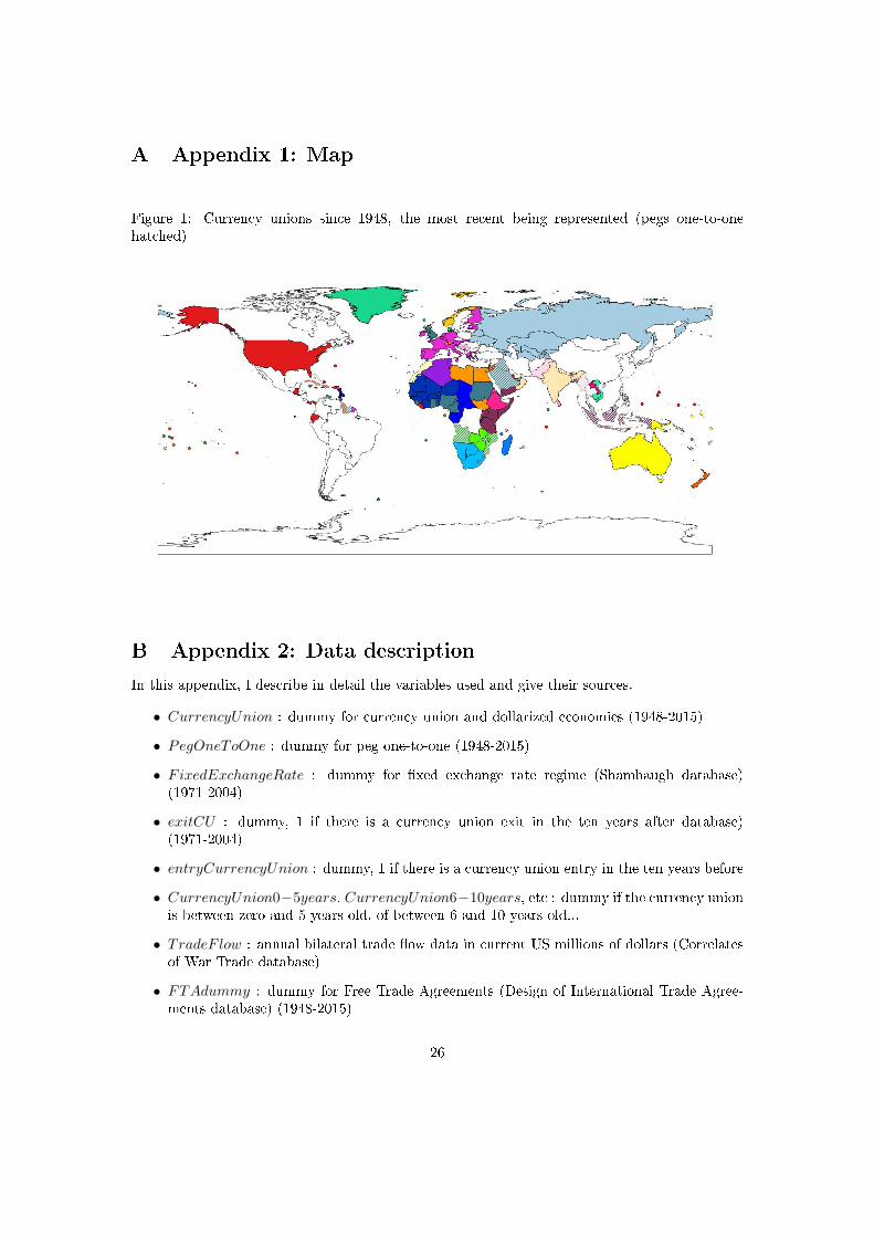
A Appendix 1: Map

Figure 1: Currency unions since 1948, the most recent being represented (pegs one-to-onehatched)

B Appendix 2: Data description

In this appendix, I describe in detail the variables used and give their sources.

• CurrencyUnion : dummy for currency union and dollarized economies (1948-2015)

• PegOneToOne : dummy for peg one-to-one (1948-2015)

• FixedExchangeRate : dummy for xed exchange rate regime (Shambaugh database)(1971-2004)

• exitCU : dummy, 1 if there is a currency union exit in the ten years after database)(1971-2004)

• entryCurrencyUnion : dummy, 1 if there is a currency union entry in the ten years before

• CurrencyUnion0−5years, CurrencyUnion6−10years, etc : dummy if the currency unionis between zero and 5 years old, of between 6 and 10 years old...

• TradeF low : annual bilateral trade ow data in current US millions of dollars (Correlatesof War Trade database)

• FTAdummy : dummy for Free Trade Agreements (Design of International Trade Agree-ments database) (1948-2015)

26

• GDPperCapita : GDP per capita in constant 2005 US dollar (World Development Indi-cators from the World Bank) (1960-2014)

• Distance : simple distance (most populated cities, km) (CEPII database "GeoDist")

• CommonBorder : dummy for common frontier (CEPII database "GeoDist")

• CommonLanguage : dummy, 1 if a language is spoken by at least 9% of the population inboth countries (CEPII database "GeoDist")

• Colony : dummy, 1 for pairs ever in colonial relationship (CEPII database "GeoDist")

• CurrentColony : dummy, 1 for pairs currently in colonial relationship (CEPII database"GeoDist")

• Population : total population (World Development Indicators from the World Bank) (1960-2014)

• Surface : Land area in square kilometer (World Development Indicators from the WorldBank)(1960-2014)

• Landlocked : dummy, if one of the two countries is landlocked (CEPII database "GeoDist")

• BothLandlocked : dummy, if the two countries are landlocked (CEPII database "GeoDist")

• Island : dummy, if one of the two countries is an island (CEPII database "GeoDist")

• BothIsland : dummy, if the two countries are islands (CEPII database "GeoDist")

with

• Prex "ln" for logarithm

• Prex "max" for maximum

• Prex "min" for minimum

27

C Appendix 3: Tables

Variable Regime Obs. Mean Std. Dev. Min Max

CommonBorderAll 3336216 0.012 0.109 0 1CU 39434 .1080286 .3104205 0 1

Peg1:1 34430 .0368283 .1883429 0 1Fixed 91732 .0431256 .203141 0 1

CommonLanguageAll 3336216 0.177 0.381 0 1CU 39434 .6588731 .4740939 0 1

Peg1:1 34430 .701946 .45741 0 1Fixed 91732 .3257969 .4686744 0 1

ColonyAll 3336216 0.01 0.098 0 1CU 39434 .0849521 .2788139 0 1

Peg1:1 34430 .0307871 .1727429 0 1Fixed 91732 .0176601 .1317135 0 1

DistanceAll 3336216 8545.405 4683.881 59.61723 19951.16CU 39434 4079.538 4342.446 59.61723 18517.37

Peg1:1 34430 6102.437 4594.335 111.0933 19227.74Fixed 91732 6995.551 4958.834 80.98481 19711.86

SurfaceAll 13032 3709523 1.24e+07 2 1.30e+08CU 3982 867813.9 3478862 2 2.74e+07

Peg1:1 1701 307632.2 410171.6 50 2381740Fixed 1194 588083.9 1313594 300 9388250

PopulationAll 13429 1.43e+08 5.50e+08 4279 7.21e+09CU 4164 3.45e+07 1.37e+08 5563 1.27e+09

Peg1:1 1758 5329419 7073528 5563 5.72e+07Fixed 1192 2.75e+07 1.30e+08 60704 1.30e+09

GDPperCapitaAll 9916 1.11e+12 4.48e+12 1.60e+07 5.81e+13CU 3010 5.23e+11 2.03e+12 1.60e+07 1.83e+13

Peg1:1 1326 2.57e+10 6.95e+10 1.12e+08 5.81e+11Fixed 1003 6.07e+10 1.66e+11 1.09e+08 2.04e+12

Table A1: Summary Statistics

28

(1)lnTradeFlow CUdollar Peg FTA

CurrencyUnion 0.502***(0.0405)

PegOneToOne 0.216***(0.0578)

FixedExchangeRate -0.0113(0.0108)

FTAdummy 0.262***(0.0113)

Constant 1.062***(0.00274)

Pair-country FE YESExporter-year FE YESImporter-year FE YESObservations 421,083R-squared 0.881F-test 20.44Prob > F 6.17e-06


Table A2: Controling for FTA with the LSDV method

29

(1) (2)lnTradeFlow Time xed eect Time and country xed eect

CurrencyUnion 0.820*** 0.498***(0.0373) (0.0345)

PegOneToOne 0.230*** 0.378***(0.0426) (0.0410)

FixedExchangeRate 0.0246** 0.00939(0.0124) (0.0119)

lnDistance -0.995*** -1.229***(0.00497) (0.00512)

CommonBorder 0.762*** 0.447***(0.0209) (0.0193)

CommonLanguage 0.471*** 0.499***(0.00888) (0.00985)

Colony 1.209*** 1.281***(0.0214) (0.0212)

CurrentColony -2.309*** -1.577***(0.186) (0.170)

FTAdummy 0.479*** 0.298***(0.0105) (0.0104)

maxlnGDPperCapita 0.959*** 0.433***(0.00243) (0.00796)

minlnGDPperCapita 0.912*** 0.641***(0.00270) (0.00768)

maxlnPopulation 0.0210*** -0.0427**(0.00345) (0.0214)

minlnPopulation 0.0471*** 0.0401*(0.00388) (0.0214)

maxlnSurface -0.127***(0.00291)

minlnSurface -0.0563***(0.00259)

Landlocked -0.382***(0.00814)

BothLandlocked 0.448***(0.0225)

Island 0.204***(0.00921)

BothIsland 0.878***(0.0201)

Year FE YES YESImporter FE NO YESExporter FE NO YESObservations 351,025 353,887F-test 119.5 5.856Prob > F 0 0.0155


Table A3: Censored maximum likelihood procedure

30

(1)

(2)

(3)

(4)

(5)

(6)

CUorPegOneToOne

Probitestimates

forcurrency

union

Marginaleect

evaluatedat

meanforCU

Probitestimates

forpeg1:1

Marginaleect

evaluatedat

meanforpeg1:1

Marginaleect

evaluatedat

meanofCUpair

Marginaleect

evaluatedat

meanofpeg1:1

pair

lnDistance

-0.789***

-0.00523***

-0.853***

-2.57e-05**

-0.180***

-0.000625***

(0.0198)

(0.000331)

(0.0493)

(1.23e-05)

(0.00612)

(0.000198)

CommonBorder

0.190***

0.00126***

-0.620***

-1.87e-05**

0.0434***

-0.000454**

(0.0522)

(0.000370)

(0.170)

(9.30e-06)

(0.0120)

(0.000183)

CommonLanguage

0.207***

0.00137***

2.021***

6.09e-05**

0.0474***

0.00148***

(0.0344)

(0.000241)

(0.138)

(2.80e-05)

(0.00787)

(0.000433)

Colony

0.293***

0.00194***

0.0710

2.14e-06

0.0670***

5.20e-05

(0.0452)

(0.000307)

(0.0830)

(2.87e-06)

(0.0105)

(6.49e-05)

CurrentC

olony

1.670***

0.0111***

0.382***

(0.0970)

(0.000976)

(0.0246)

FTAdummy

0.549***

0.00364***

-0.772***

-2.33e-05*

0.125***

-0.000565***

(0.0422)

(0.000312)

(0.119)

(1.22e-05)

(0.0100)

(0.000174)

maxlnGDPperCapita

0.198***

0.00131***

-0.255***

-7.69e-06**

0.0452***

-0.000187***

(0.0196)

(0.000145)

(0.0265)

(3.83e-06)

(0.00461)

(6.18e-05)

minlnGDPperCapita

-0.0347***

-0.000230***

-0.177***

-5.33e-06**

-0.00793***

-0.000129***

(0.0110)

(7.33e-05)

(0.0243)

(2.66e-06)

(0.00253)

(4.08e-05)

maxlnPopulation

-0.191***

-0.00126***

0.689***

2.08e-05**

-0.0436***

0.000504***

(0.0278)

(0.000194)

(0.0638)

(9.91e-06)

(0.00646)

(0.000154)

minlnPopulation

-0.0790***

-0.000524***

0.171***

5.14e-06*

-0.0181***

0.000125***

(0.0158)

(0.000109)

(0.0347)

(2.69e-06)

(0.00361)

(4.23e-05)

maxlnSurface

0.343***

0.00227***

-0.227***

-6.83e-06**

0.0784***

-0.000166***

(0.0144)

(0.000151)

(0.0375)

(3.25e-06)

(0.00380)

(5.15e-05)

minlnSurface

-0.0629***

-0.000417***

0.0194

5.86e-07

-0.0144***

1.42e-05

(0.00892)

(6.48e-05)

(0.0205)

(6.70e-07)

(0.00208)

(1.54e-05)

Observations

93,318

93,318

92,962

92,962

93,318

92,962

Standard

errors

inparentheses

***p<0.01,**p<0.05,*p<0.1

TableA4:Propensity

toadoptthecurrency,orto

peg,to

main

anchor

31

Documents

Disentangle the E ects on Trade: Currency Union, Peg … · I study a two-country theoretical world economy with à ... This reinforces the importance of ... lot of papers later on