Embed Size (px)
Citation preview
arX
iv:1
301.
6757
v1 [
astr
o-ph
.CO
] 28
Jan
201
3Mon. Not. R. Astron. Soc.000, 000–000 (0000) Printed 24 January 2018 (MN LATEX style file v2.2)
Disentangling satellite galaxy populations using orbit tracking insimulations
Kyle A. Oman1,⋆, Michael J. Hudson1,2, Peter S. Behroozi3
1 Department of Physics and Astronomy, University of Waterloo, Waterloo, Ontario, N2L 3G1, Canada2 Perimeter Institute for Theoretical Physics, Waterloo, Ontario, N2L 2Y5, Canada3 Kavli Institute for Particle Astrophysics and Cosmology; Physics Department, Stanford University; Department of Particle Physics andAstrophysics, SLAC National Accelerator Laboratory, Stanford, CA 94305
24 January 2018
ABSTRACTPhysical processes regulating star formation in satellitegalaxies represent an area of ongoingresearch, but the projected nature of observed coordinatesmakes separating different popula-tions of satellites (with different processes at work) difficult. The orbital history of a satellitegalaxy leads to its present-day phase space coordinates; wecan also work backwards and usethese coordinates to statistically infer information about the orbital history. We use mergertrees from the MultiDark Run 1 N-body simulation to compile acatalogue of the orbits ofsatellite haloes in cluster environments. We parametrize the orbital history by the time sincecrossing within 2.5rvir of the cluster centre and use our catalogue to estimate the probabilitydensity over a range of this parameter given a set of present-day projected (i.e. observable)phase space coordinates. We show that different populations of satellite haloes, e.g. infalling,backsplash and virialized, occupy distinct regions of phase space, and semi-distinct regions ofprojected phase space. This will allow us to probabilistically determine the time since infall ofa large sample of observed satellite galaxies, and ultimately to study the effect of orbital his-tory on star formation history (the topic of a future paper).We test the accuracy of our methodand find that we can reliably recover this time within±2.58 Gyr in 68 per cent of cases byusing all available phase space coordinate information, compared to±2.64 Gyr using onlyposition coordinates and±3.10 Gyr guessing ‘blindly’, i.e. using no coordinate information,but with knowledge of the overall distribution of infall times. In some regions of phase space,the accuracy of the infall time estimate improves to±1.85 Gyr. Although we focus on timesince infall, our method is easily generalizable to other orbital parameters (e.g. pericentricdistance and time).
Key words: galaxies: kinematics and dynamics, galaxies: clusters: general, galaxies: haloes
1 INTRODUCTION
We know that galaxies in clusters are typically more ‘red anddead’than their counterparts in the field (Hogg et al. 2004; Baloghet al.2004), as well as dominantly elliptical (rather than spiral, seeDressler 1980). This is thought to be due to a mechanism or com-bination of mechanisms that halt the collapse of cold gas into starsin a satellite galaxy as it orbits within a deep potential well – eitherby heating or removing the gas or by preventing the cooling ofad-ditional gas and consuming the existing supply. Some renownedmechanisms include ram pressure stripping (e.g. Gunn & Gott1972; Abadi et al. 1999; Jachym et al. 2007; Smith et al. 2010b),tidal stripping (Mayer et al. 2006), harassment (Moore et al. 1996;
Smith et al. 2010a), strangulation (Larson et al. 1980; Balogh et al.2000) and mergers (Toomre & Toomre 1972; Cox et al. 2006).Internal quenching mechanisms have also been proposed – e.g.shock heating (Birnboim & Dekel 2003; Dekel & Birnboim 2006),AGN heating (Croton et al. 2006; McNamara et al. 2006), see alsoGabor et al. (2010) – which, while unable to account for the dif-ference between field and cluster galaxies, may each contribute toincreasing the red fraction in both environments.
It has so far been found difficult to produce a semi-analyticmodel for quenching that both reproduces the observed star forma-tion rate (SFR) distribution in clusters (Wetzel et al. (2012), but seeWeinmann et al. (2010) for some recent improvements). However,all the environmental quenching mechanisms listed above have atleast one common characteristic : each is sensitive to the path takenthrough the cluster. Tidal stripping is strongest near the cluster cen-
c© 0000 RAS

2 K. A. Oman, M. J. Hudson & P. S. Behroozi
tre. Ram pressure stripping varies with the local density ofhot clus-ter gas and the relative velocity of the satellite, both of which varyradially in the cluster. Mergers are more probably in the outskirtsof clusters. Harassment is most effective during high speedencoun-ters, which occur near the cluster core. Strangulation is triggeredby the removal of the halo gas of the satellite, obsensibly via oneof the aforementioned mechanisms. An environmental quenchingmodel can therefore reasonably be expected to depend on the pre-vious positions and velocities, or more concisely the orbital history,of satellite galaxies.
The orbital history of a galaxy is not directly observable; if wehope to compare environmental quenching models to observationaldata, we need some way to characterize the orbit of an observedgalaxy. We might parametrize the orbital history of a galaxyin anyof a number of ways – for instance by the time since infall intothecluster potential, the distance of closest approach to the cluster cen-tre or the number of orbits completed since infall – then attempt tofind correlations between these parameters and observablesusingN-body simulation data. The observables we consider available arethe distance between the satellite and the cluster centre projectedon to the plane of the sky and the component of the velocity of thesatellite relative to the cluster centre along the line of sight (LoS). Insome nearby clusters it may also be possible to obtain distances tothe cluster centre and the satellite via direct distance measurements(e.g. Tully-Fisher relation, surface brightness fluctuations, SNIa lu-minosities, etc.), but in general these will be much less precise thanthe other two coordinates – we will consider this information inac-cessible.
Several authors (Gao et al. 2004; Wang et al. 2011;De Lucia et al. 2012; Taranu et al. 2012) have shown that thepresent radial distance from the cluster centre is negativelycorrelated to the time since infall into the cluster and other orbitalparameters. Gill et al. (2005) were amongst the first to comparethe velocity distributions of different satellite populations (seealso Wang et al. 2005), and more recently Mahajan et al. (2011)presented a method for separating satellite populations based on,amongst other parameters, their LoS velocities.
This paper presents our method for reconstructing theparametrized orbital history of a satellite galaxy based onitspresent-day observable phase space coordinates; we defer its appli-cations to future papers. Here, we focus on one parameter – the timesince infall on to a cluster-sized host – but stress that our method iseasily adapted to other parameter choices. The time since the satel-lite first passed pericentre on its orbit in the cluster and the distanceof closest approach to the cluster centre are two examples ofotherparameter choices that will be of interest in future applications ofour method.
In section 2 we describe the N-body simulation data and itsconversion into halo catalogues and merger trees. In section 3 wepresent the method used convert the merger trees into our cata-logues of satellite orbits, and to a probability distribution functionof times since infall given a pair of coordinates in phase space.In section 4 we discuss the importance of LoS velocity data indis-criminating between different populations of satellites.We summa-rize in section 5.
We assume the same cosmology used in the Bolshoi andMultidark Run 1 simulations withΩm = 0.27, ΩΛ = 0.73,Ωb = 0.0469, ns = 0.95, h0 = 0.70, σ8 = 0.82 (Prada et al.2012).
2 SIMULATIONS
To obtain a large sample of satellite orbits, we use the output ofthe MultiDark Run 1 (MDR1) dark matter only simulation with1 Gpch−1 box side length,20483 particles, current cosmology(WMAP5/WMAP7), 8.7 × 10⁹h−1 M⊙ mass resolution and 7kpc force resolution. The simulation was run fromz = 65 to thepresent; the majority of snapshots are output at even intervals inscale factora with some irregular intervals at smalla. The resolu-tion in scale factor is of 0.0304 beforea ∼ 0.7 (z ∼ 0.43) anddoubles to 0.0152 afterwards (corresponding to a time resolutionof about 0.210 Gyr atz = 0). This is taken into account in ourdiscussion below. Full details of the simulation parameters are de-scribed in Prada et al. (2012). The simulation snapshots were pro-cessed by theROCKSTAR halo finder (Behroozi et al. 2011a) andthe merger tree code presented in Behroozi et al. (2011b). Topro-duce the data used in this paper, the merger tree code was slightlymodified so that a halo may contain satellite haloes at distances ofup to 2.5 times its virial radius (rvir = r360b) from its centre; thedefault code finds satellites within only 1.0 virial radii. This allowsus to track satellites out to the largest apocentric distances whichMamon et al. (2004) (see also Gill et al. 2005; Balogh et al. 2000;Ludlow et al. 2009) show to be about∼ 2.5r200c(∼ 2.2r360b) byusing host-satellite linking as a proxy for cluster membership.
In the following discussion, we will denote full 6D cluster-centric coordinates(r, v). The position and velocity centre of a halois determined by averaging the positions and velocities of the sub-set of halo particles which minimizes the expected Poisson error inthe coordinates, i.e. the particles occupying the region ofhighest lo-cal density (for more detail on how the coordinates are determinedby the halo finder, we refer the interested reader to Behrooziet al.2011a,§3.5.1).
Projected coordinates will be denoted(R, V ). Projection isdone along the arbitrarily chosen third (z-)axis of the simulationbox and includes a correction to the velocities to account for theHubble flow. With this correction, the simulated velocity differ-ences can be directly compared to observation data, where ve-locity differences would presumably be measured using a red-shift difference. The projected distance between two points isR12 =
√
(r2,x − r1,x)2 + (r2,y − r1,y)2 and the relative veloc-ity of point 2 with respect to point 1 isV12 = |(v2,z − v1,z) +H(r2,z − r1,z)|. Note thatV ≥ 0; this encodes our assumptionthat the distances to the two points are not known precisely,so onlythe magnitude of their relative velocity can be determined.
For ease of comparison between satellites of different hosts,all spatial coordinates are normalized to the virial radiusrvir of thehost halo, which is defined using the formula of Bryan & Norman(1998): the radius enclosing a region with an overdensity of360times the background density atz = 0. For readers more accus-tomed to normalization byr200c, an approximate conversion atz = 0 is r200c
rvir∼ 1.13. All velocity coordinates are normalized
to the rms velocity dispersionσ of the host halo, measured in 3D.
3 METHOD
First, the orbital history of a satellite and its host atz = 0 are de-termined. Then the infall time of the satellite into that host halo isdefined as the earliest time at which the satellite’s progenitor iden-tifies thez = 0 host’s progenitor as its host. A host-satellite pairmay be identified as soon as the satellite is within 2.5 times thevirial radius of the host; though other criteria must still be met,
c© 0000 RAS, MNRAS000, 000–000
Disentangling satellite galaxy populations 3
10 11 12 13 14 15log10Minfall/M⊙
102
103
104
105
106
N
Nall=509075Npast=216826
N0.0−0.25=59971N0.25−0.50=96508N0.50−0.75=44886N0.75−1.00=15461
mass cut Mcut
all satssats past periperi=0.0-0.25 rvir0.25-0.50.5-0.750.75-1.0
10-2 10-1 100 101
rsat [Mpc]100
101
102
103
104
105
106
numbe
r den
sity [M
pc−1] all satellites
µ=10−3.0−10−2.510−2.5−10−2.010−2.0−10−1.510−1.5−10−1.010−1.0−10−0.510−0.5−100.0
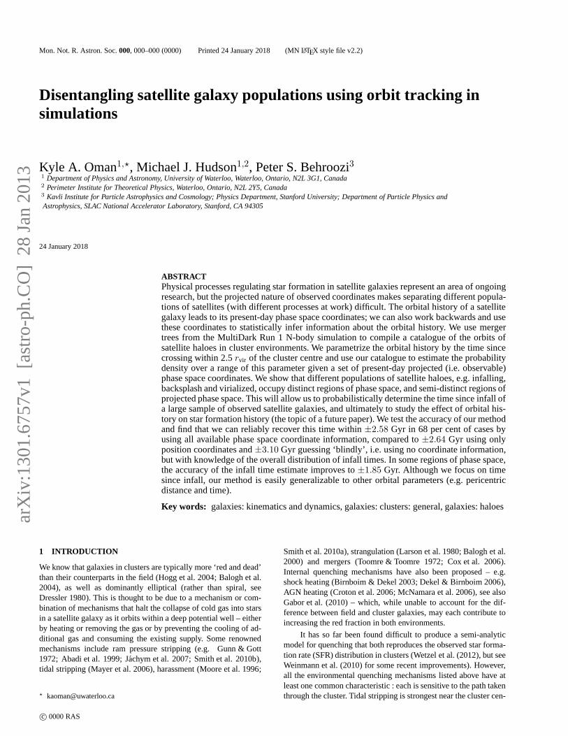
Figure 1. These two figures provide a measure of the importance of resolution effects in our analysis; see section 3 and§4.4 for discussion.Left panel:The mass function of all satellite haloes in our initial sample (dotted black line) and the mass function of satellite haloes that have experienced at least onepericentric passage (solid black line), where in both casesthe masses are measured at the time of infall on to their host.The coloured lines separate the satellitesthat have experienced a pericentric passage into bins of pericentric distance, as labelled. The total number of satellites contributing to each mass function arelabelledN . We impose a mass cut as indicated by the thick vertical line (Mcut = 1011.9 M⊙), yielding a sample which is as complete as reasonably possibleaboveMcut. Right panel: Number density as a function of satellite radial position for various mass ratiosµ, where the mass of the satellite is measured at thetime of infall. The host halos have masses≥ 1014 M⊙. Satellites with low mass ratios are underabundant toward the centre of the cluster environment.
as outlined in Behroozi et al. (2011b), in practice these areusuallymet immediately when the satellite crosses within2.5rvir . Only theorbital history with respect to the final (z = 0) host is considered,and in cases where a satellite has a hierarchy of hosts, intermediatehosts are ignored and the satellite identifies the largest asits host;in other words, the present work ignores “group pre-processing”.Hosts are selected to be “cluster-sized”, which we define as ahalomass> 1014 M⊙. With the MDR1 dataset, this yields a catalogueof ∼ 570, 000 satellite orbits belonging to∼ 24, 500 differenthosts.
To ensure a sample complete in satellite mass, and that weare minimally sensitive to artificial disruption of satellite haloes,we impose a mass cut atMcut = 1011.9 M⊙, where the mass ismeasuredat the time of infall. Using the stellar-to-halo mass ratiosoutlined in Behroozi et al. (2012), this corresponds to a cutin stel-lar mass at∼ 1010.3 M⊙. The left panel of Fig. 1 shows the massfunction for all satellites, and for satellites that have experienced atleast one pericentric passage in bins of proximity of pericentric pas-sage. Our mass cut is safely above the mass resolution limit of thesimulation. As in essentially all cosmological simulations, MDR1halos experience artifical disruption in high density environments(Kitzbichler & White 2008; Klypin et al. 1999). This is the reasonfor the underabundance of lower mass satellites that have experi-enced a close approach to a cluster centre (blue curve in Fig.1,left panel). From these mass functions, we estimate that less than20% of halos with masses above our mass cut and pericentric dis-tances in the range0.0 − 0.25rvir have been artificially disrupted.Most of the artificially disrupted satellites are in the massrange1011.9 − 1013.1 M⊙. We estimate that these missing satellites ac-count for less than 4% of the total halo population above our masscut. The right panel of Fig. 1 shows the number density of satellitehalos as a function of radial position for bins of satellite mass rela-tive to the host halo. Observations constrain the slope of this powerlaw relation to be between−1.7 and−1.5, regardless of mass ra-tio (Tinker et al. 2012). The slopes shown in Fig 1 are somewhatsteeper at about−1.9 for mass ratioµ = 10−0.5 − 100. The rea-
son for this steeper slope is not precisely known, but the higherresolution Bolshoi simulation exhibits the same slope of−1.9 sowe surmise that it is not due to a resolution effect. The key featurethat we wish to highlight is that the slope (and shape) of thisrela-tionship is mass ratiodependent in our dataset, with satellites thatare smaller relative to their host being less abundant closer to thecentre of the host. The underabundances of satellites highlightedby each panel of Fig. 1 are due to the same population of satellites;those which have orbited to within. 0.25rvir of their host and havea mass. 1013.1 M⊙. See§4.4 for a discussion of the impact ofthese missing satellites on our results.
We impose one final cut, removing satellites that existed forless than 3 simulation snapshots before falling into a cluster. Thisprevents haloes near the mass resolution limit of the simulationfrom appearing suddenly inside a cluster and being assignedmean-ingless infall times. The remaining 242,790 satellites were binnedin 100 projected position bins in0.0 ≤ R/rvir ≤ 2.5 and 100 pro-jected velocity bins in0.0 ≤ V/σ ≤ 2.0. The set of infall timesin each bin was used to create a probability distribution function(PDF) of infall times for each bin.
4 RESULTS
Before applying our PDFs to modelling environmental quenching(which will be the focus of a future paper), we should have an un-derstanding of a few systematic effects inherent in the method pre-sented in section 3. We will discuss the impact of projectingthedata in both the radial and velocity coordinates in§4.1. In§4.2 wewill present the PDFs and discuss some of their features. In§4.3 wediscuss the effects of both host and satellite mass on the distributionof satellites in phase space. Finally, in§4.4 we discuss the impactof resolution effects on our results.
c© 0000 RAS, MNRAS000, 000–000
4 K. A. Oman, M. J. Hudson & P. S. Behroozi
4.1 Projection effects
While a simulation provides accurate values for all six phase spacecoordinates of an object, a typical astronomical observation canonly measure three. The right ascension and declination give twospatial coordinates (the distance is unknown), while comparing thespectra of two objects can give the difference in velocity betweenthem, but only for motion in a direction along the LoS. Since weultimately wish to infer properties of observed objects from theircoordinates, we must restrict our knowledge of simulated objectsto these same coordinates. This can be achieved by ignoring oneof the spatial coordinates of the simulation box – in our case, thethird – and considering only the velocity coordinate correspondingto the ignored spatial coordinate. Additionally, we include a correc-tion to the projected velocity to account for the Hubble flow.Thistransformation applied to the spatial coordinates of a point x andits velocityu relative to a reference pointy and its velocityw canbe expressed:
r = (x− y) = (x1 − y1, x2 − y2, x3 − y3)
⇒ R = (x1 − y1, x2 − y2)
v = (u−w) = (u1 − w1, u2 − w2, u3 −w3)
⇒ V = (|(u3 − w3) +H(x3 − y3)|)
We predict the effect of projection on the radial coordinatebyconsidering a random uniform distribution of points on a spher-ical shell. For this distribution the relationship betweenthe ac-tual (r) and projected (R) radial coordinates is characterized by
〈Rr〉 = π
4±
√
2
3− π2
16∼ 0.79 ± 0.22 (1σ scatter). In our sam-
ple of satellite galaxies, we find that〈Rr〉 agrees with this pre-
diction to within 1%, both in the mean and in the scatter. Theprojected radial coordinate tracks the 3D radial coordinate moreclosely and more consistently at larger projected radii; atR ∼ rvir,〈Rr〉 ∼ 0.83 ± 0.17 while atR ∼ 0.1rvir , 〈Rr 〉 ∼ 0.51 ± 0.31.
The observed velocity coordinate does not have as straightforwarda relationship with the actual quantity of interest – the radial com-ponent of the velocity difference between two points – but the in-formation about two components is lost instead of one, so we ex-pect a much larger typical difference between projected velocityand true velocity. We also lose the sign of the one remaining com-ponent of velocity since, without knowledge of the distances to thetwo points, we cannot know whether the distance between themisincreasing or decreasing.
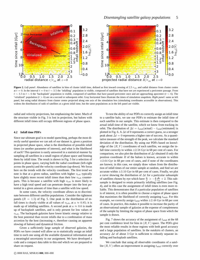
The left panel of Fig. 2 shows the distribution of satellite infalltimes1 as a function of radial distance from the host centremea-sured at z = 0 before projection. Satellites that have recent infalltimes (near the top of the diagram) are necessarily concentratednear the edge of our definition of the cluster at 2.5rvir; they havenot had enough time to move anywhere else. A typical crossingtime for our sample of clusters is about 6-8 Gyr, so most satellitesthat fell in 3-4 Gyr ago are near the centre of the host. Note thatthis seemingly long crossing time is due to our definition of theedge of the cluster at 2.5rvir; the typical time to cross fromrvir topericentre and back torvir is about 2 Gyr. The satellite also spends asignificant amount of time outside the virial radius after this initialcrossing; it takes a further∼1 Gyr for a typical satellite to reachapocentre after making its first outbound crossing ofrvir.
1 The infall times produced by the method of section 3 occur at discretetimes – those of the simulation snapshots. For the purposes of visualizationonly, some scatter was added to the times.
There is a spread in the time taken to reach pericentre and theradii of the pericentres caused by the variety of possible orbits anddetails of the host potentials. The first apocentre after infall typi-cally occurs after about 6 Gyr; the population of objects betweenfirst pericentre and apocentre is termed ‘backsplash’. Satellites withinfall times earlier than∼ 7 Gyr have less distinct features in theirdistribution due to the increasing impact of variations in orbital his-tory, but the majority are confined within∼ 1 rvir; we call this pop-ulation ‘virialized’. We note an overall decreasing numberof satel-lites with increasing time since infall. Some satellites with earlyinfall times are disrupted by tidal interactions and do not appear inour merger trees. In other cases two infalling satellites may mergeand appear in the trees as a single satellite. Finally, some halos maynot host a galaxy. These three effects mean that observations ofsatellite galaxies around a cluster do not correlate perfectly withthe distribution of dark matter halos around that cluster; this needsto be taken into account when applying our method to a sample ofobserved galaxies, but does not impact the method itself. There isone other contribution to the decrease in number of satellites withincreasing time since infall. Because our mass limit of1011.9 M⊙isrelatively large, at early times haloes above this limit were some-what rarer.
The right panel of Fig. 2 shows the effect of projection in theradial coordinates on the same distribution as in the left panel. Fea-tures are shifted somewhat to lower radii (consistently with ourexpectation of〈R
r〉 = π
4) and broadened by the scatter about
this mean deformation. All the populations and features discussedabove are still identifiable. One notable omission from thisdiagramis any foreground/background objects, which are common in obser-vational samples, that could be confused with the satellitepopula-tions.
There is one other important effect to consider when inter-preting Fig. 2 (and others involving infall times). As a hosthaloaccretes mass, its virial radius grows (slowly, except in the case ofmajor mergers). Because of this, an orbiting satellite may appear tomove further in coordinates scaled torvir than it otherwise would asthe coordinates grow around it. This does not have a large impacton the positions, but contributes some of the scatter in the radial co-ordinate. One might consider choosing some radius that is constantwith time to scale each halo, but other choices, such as the virialradius at the last snapshot, also introduce similar effects.
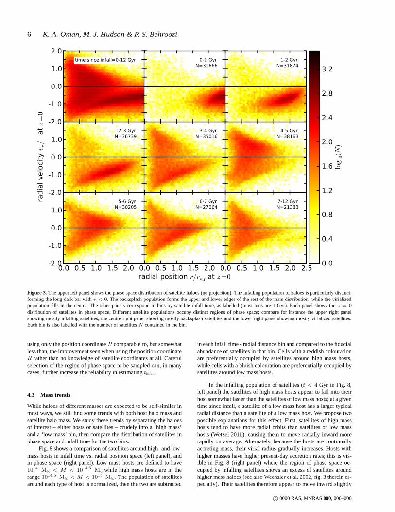
Next, we consider the effect of projection on the velocity co-ordinates. The upper left panel of Fig. 3 shows the distribution ofsatellite haloes in phase space atz = 0. A typical halo would, givenenough time, progress from large radii and low velocities down tolow radii and high negative velocities, then switch to high positivevelocity as it passes pericentre. From there it follows a series of pro-gressively shrinking concentric semicircles or chevrons,jumpingfrom negative to positive velocity at each pericentric passage (fora more in depth theoretical background, see Bertschinger 1985, es-pecially fig. 6 therein). This normal progression is well representedby the distribution of our halo sample, however the individual or-bital ‘shells’ are not visible since they overlap, and we only expect1-2 shells given the orbital timescales and ages of these systems.Also, close encounters redistribute some haloes off this idealizedtrack.
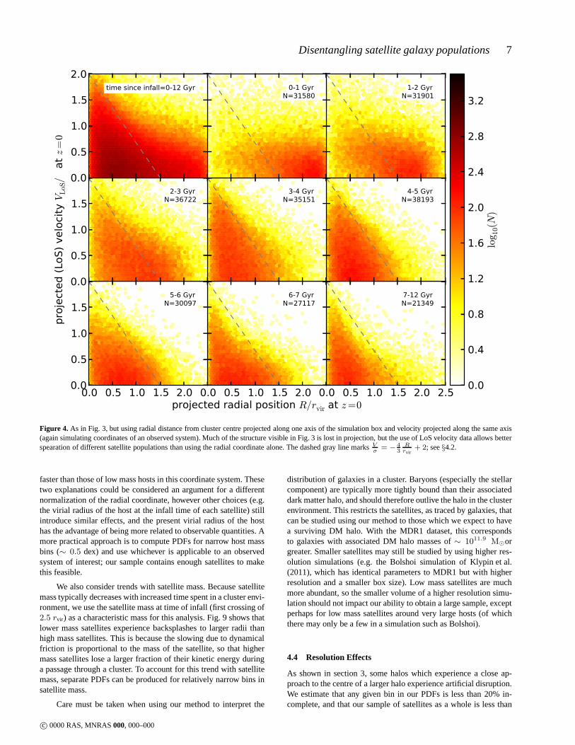
Based on this expected movement through phase space intime, satellite haloes with different infall times should occupy dif-ferent regions of phase space. This is shown in Fig. 3, where thephase space distribution of haloes is plotted for a variety of binsin infall time. Fig. 4 shows the same binned distributions, but inprojected coordinates, simultaneously showing the effects of both
c© 0000 RAS, MNRAS000, 000–000
Disentangling satellite galaxy populations 5
0.0 0.5 1.0 1.5 2.0 2.5radial distance r/rvir at z=0
12
10
8
6
4
2
0
time since infall [Gyr] Infall
ing
Backsplash
Virialized
First Pericenter
Apocenter
00.10.20.30.40.60.811.21.523
infall redshift z
0.00.40.81.21.62.02.42.83.2
log 1
0(N
)
0.0 0.5 1.0 1.5 2.0 2.5projected radial distance R/rvir at z=0
12
10
8
6
4
2
0
time sinc
e infall [G
yr]
00.10.20.30.40.60.811.21.523
infall reds
hift z
0.00.40.81.21.62.02.42.83.2
log 1
0(N
)
Figure 2. Left panel: Abundance of satellites in bins of cluster infall time, defined as first inward crossing of 2.5rvir , and radial distance from cluster centreat t = 0. In the intervalt = 0 to t ∼ 3.5 the ‘infalling’ population is visible, composed of satellites that have not yet experienced a pericentre passage. Fromt ∼ 3.5 to t ∼ 6 the ‘backsplash’ population is visible, composed of satellites that have passed pericentre once and are approaching apocentre (t ∼ 6). The‘virialized’ population (t > 6) are on a second or subsequent orbit. Gray horizontal lines illustrate the times of simulation snapshots.Right panel: same as leftpanel, but using radial distance from cluster centre projected along one axis of the simulation box (simulating coordinates accessible in observations). Thiswidens the distribution of radii of satellites at a given infall time, but the same populations as in the left panel are visible.
radial and velocity projections, but emphasizing the latter. Much ofthe structure visible in Fig. 3 is lost in projection, but haloes withdifferent infall times still occupy different regions of phase space.
4.2 Infall time PDFs
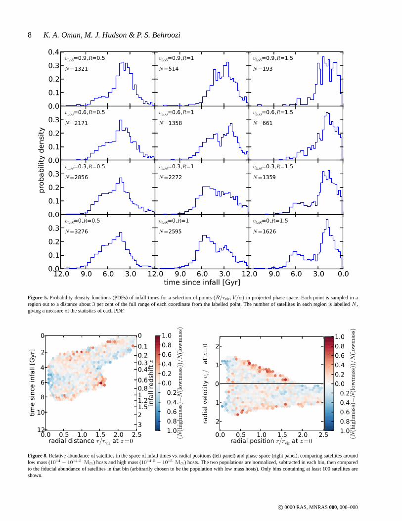
Since our ultimate goal is to model quenching, perhaps the most di-rectly useful question we can ask of our dataset is, given a positionin projected phase space, what is the distribution of possible infalltimes (or another parameter of interest), and what is the likelihoodof each? This question is easily answered in a statistical manner bysampling all satellites in a small region of phase space and binningthem by infall time. The result is shown in Fig. 5 for a selection ofpoints in phase space, varying both the radial coordinate (left-rightacross the panels) and the velocity coordinate (up-down). We focushere on the trends with the velocity coordinate. The first trend wenote is that at a given radius, satellites with highervLoS typicallyhave slightly more recent infall times than their lowvLoS counter-parts. This is because a satellite with highvLoS is more likely tohave a high total speed and can penetrate deeper into the hostpo-tential in a given amount of time than a satellite with low speed.
In some cases, the velocity coordinate allows us to discrimi-nate between different satellite populations. Consider the rightmostpanels (R = 1.5) of Fig. 5. One peak in the distribution of in-fall times is clearly visible at all values ofvLoS, at a ≈ 0.85; it ismade up of infalling satellites. A second peak ata ≈ 0.6 is madeup of backsplash satellites, and is only present for low values ofvLoS. The backspash galaxies have lower kinetic energy relativetothe host potential than recent infalls due to a combination of massaccretion by the host (increasingσ, therefore causing an apparentslowing of haloes) and dynamical friction.
Given a sufficiently large sample of observed galaxies, thePDFs we have created will allow us to statistically assign aninfalltime to each one using all the available dynamical information anda meaningful uncertainty in our assignment. We have developed acode and a compact data table to this end which we are preparedtoshare on request.
To test the ability of our PDFs to correctly assign an infall timeto a satellite halo, we use our PDFs to estimate the infall time ofeach satellite in our sample. This estimate is then comparedto theactual infall time of the satellite, which we know from tracking itsorbit. The distribution of∆t = tinfall(actual) − tinfall(estimated) isplotted in Fig. 6. A∆t of 0 represents a correct guess, so a strongerpeak about∆t = 0 represents a higher rate of success. As a quanti-tative measure of the strength of the peak, we calculate the standarddeviation of the distribution. By using our PDFs based on knowl-edge of the(R, V ) coordinates of each satellite, we assign the in-fall time correctly to within±2.58 Gyr in 68 per cent of cases. Forcomparison, we also plot the distribution of∆t obtained if only theposition coordinateR of the haloes is known, accurate to within±2.64 Gyr in 68 per cent of cases, and if none of the coordinatesare known; in this case, we simply draw values from the distribu-tion of infall times of our entire sample at random, and find weareaccurate within±3.10 Gyr in 68 per cent of cases. Finally, we plota curve showing the distribution of∆t for a particular subsampleof satellites chosen by eye which haveV
σ> − 4
3
R
rvir+ 2. This sub-
sample is designed to retain primarily infalling satellites (see Fig.4), and in this case the assignment of infall times is even more re-liable. This demonstrates that if a particular population of satellitesis of interest, it is often possible to choose a region of phase spacethat maximises the likelihood of correctly assigningtinfall. For thisexample, we correctly assigntinfall within ±2.48 Gyr in 68 per centof cases. In practice, this makes it possible to increase thepurity ofan observational sample of galaxies at the expense of completenessof the sample by limiting the region of phase space from whichthesample is drawn.
Fig. 7 shows the accuracy of the assignment oftinfall at the 68per cent confidence level for bins in(R,V ) space. The PDFs givethe most reliable results in those regions with both good accuracyand a large population of satellites. In the outskirts of clusters, anaccuracy∆t of about 3 Gyr is sufficient to robustly separate in-falling and backsplash satellites.
We conclude that using all observable coordinates of a satel-lite (R, V ) offers an improvement in assigningtinfall correctly over
c© 0000 RAS, MNRAS000, 000–000
6 K. A. Oman, M. J. Hudson & P. S. Behroozi
0.0 0.5 1.0 1.5 2.0 2.5
7-12 GyrN=21383
0.0 0.5 1.0 1.5 2.0 radial position r/rvir at z=0
6-7 GyrN=27064
0.0 0.5 1.0 1.5 2.0 -2.0
-1.0
0.0
1.0
5-6 GyrN=30205
4-5 GyrN=38163
3-4 GyrN=35016
-2.0
-1.0
0.0
1.0
radial veloc
ity v
r/σ at z
=0
2-3 GyrN=36739
1-2 GyrN=31874
0-1 GyrN=31666
-2.0
-1.0
0.0
1.0
2.0time since infall=0-12 Gyr
0.0
0.4
0.8
1.2
1.6
2.0
2.4
2.8
3.2
log 1
0(N)
Figure 3. The upper left panel shows the phase space distribution of satellite haloes (no projection). The infalling population of haloes is particularly distinct,forming the long dark bar withv < 0. The backsplash population forms the upper and lower edges of the rest of the main distribution, while the virializedpopulation fills in the centre. The other panels correspond to bins by satellite infall time, as labelled (most bins are 1 Gyr). Each panel shows thez = 0distribution of satellites in phase space. Different satellite populations occupy distinct regions of phase space; compare for instance the upper right panelshowing mostly infalling satellites, the centre right panel showing mostly backsplash satellites and the lower right panel showing mostly virialized satellites.Each bin is also labelled with the number of satellitesN contained in the bin.
using only the position coordinateR comparable to, but somewhatless than, the improvement seen when using the position coordinateR rather than no knowledge of satellite coordinates at all. Carefulselection of the region of phase space to be sampled can, in manycases, further increase the reliability in estimatingtinfall.
4.3 Mass trends
While haloes of different masses are expected to be self-similar inmost ways, we still find some trends with both host halo mass andsatellite halo mass. We study these trends by separating thehaloesof interest – either hosts or satellites – crudely into a ‘high mass’and a ‘low mass’ bin, then compare the distribution of satellites inphase space and infall time for the two bins.
Fig. 8 shows a comparison of satellites around high- and low-mass hosts in infall time vs. radial position space (left panel), andin phase space (right panel). Low mass hosts are defined to have1014 M⊙ < M < 1014.5 M⊙while high mass hosts are in therange1014.5 M⊙ < M < 1015 M⊙. The population of satellitesaround each type of host is normalized, then the two are subtracted
in each infall time - radial distance bin and compared to the fiducialabundance of satellites in that bin. Cells with a reddish colourationare preferentially occupied by satellites around high masshosts,while cells with a bluish colouration are preferentially occupied bysatellites around low mass hosts.
In the infalling population of satellites (t < 4 Gyr in Fig. 8,left panel) the satellites of high mass hosts appear to fall into theirhost somewhat faster than the satellites of low mass hosts; at a giventime since infall, a satellite of a low mass host has a larger typicalradial distance than a satellite of a low mass host. We propose twopossible explanations for this effect. First, satellites of high masshosts tend to have more radial orbits than satellites of low masshosts (Wetzel 2011), causing them to move radially inward morerapidly on average. Alternately, because the hosts are continuallyaccreting mass, their virial radius gradually increases. Hosts withhigher masses have higher present-day accretion rates; this is vis-ible in Fig. 8 (right panel) where the region of phase space oc-cupied by infalling satellites shows an excess of satellites aroundhigher mass haloes (see also Wechsler et al. 2002, fig. 3 therein es-pecially). Their satellites therefore appear to move inward slightly
c© 0000 RAS, MNRAS000, 000–000
Disentangling satellite galaxy populations 7
0.0 0.5 1.0 1.5 2.0 2.5
7-12 GyrN=21349
0.0 0.5 1.0 1.5 2.0 projected radial position R/rvir at z=0
6-7 GyrN=27117
0.0 0.5 1.0 1.5 2.0 0.0
0.5
1.0
1.5
5-6 Gyr
N=30097
4-5 GyrN=38193
3-4 GyrN=35151
0.0
0.5
1.0
1.5
proj
ecte
d (L
oS) v
eloc
ity V
LoS/σ
at z
=0
2-3 GyrN=36722
1-2 GyrN=31901
0-1 GyrN=31580
0.0
0.5
1.0
1.5
2.0time since infall=0-12 Gyr
0.0
0.4
0.8
1.2
1.6
2.0
2.4
2.8
3.2
log 1
0(N
)
Figure 4. As in Fig. 3, but using radial distance from cluster centre projected along one axis of the simulation box and velocity projected along the same axis(again simulating coordinates of an observed system). Muchof the structure visible in Fig. 3 is lost in projection, but the use of LoS velocity data allows betterspearation of different satellite populations than using the radial coordinate alone. The dashed gray line marksV
σ= − 4
3
Rrvir
+ 2; see§4.2.
faster than those of low mass hosts in this coordinate system. Thesetwo explanations could be considered an argument for a differentnormalization of the radial coordinate, however other choices (e.g.the virial radius of the host at the infall time of each satellite) stillintroduce similar effects, and the present virial radius ofthe hosthas the advantage of being more related to observable quantities. Amore practical approach is to compute PDFs for narrow host massbins (∼ 0.5 dex) and use whichever is applicable to an observedsystem of interest; our sample contains enough satellites to makethis feasible.
We also consider trends with satellite mass. Because satellitemass typically decreases with increased time spent in a cluster envi-ronment, we use the satellite mass at time of infall (first crossing of2.5 rvir) as a characteristic mass for this analysis. Fig. 9 shows thatlower mass satellites experience backsplashes to larger radii thanhigh mass satellites. This is because the slowing due to dynamicalfriction is proportional to the mass of the satellite, so that highermass satellites lose a larger fraction of their kinetic energy duringa passage through a cluster. To account for this trend with satellitemass, separate PDFs can be produced for relatively narrow bins insatellite mass.
Care must be taken when using our method to interpret the
distribution of galaxies in a cluster. Baryons (especiallythe stellarcomponent) are typically more tightly bound than their associateddark matter halo, and should therefore outlive the halo in the clusterenvironment. This restricts the satellites, as traced by galaxies, thatcan be studied using our method to those which we expect to havea surviving DM halo. With the MDR1 dataset, this correspondsto galaxies with associated DM halo masses of∼ 1011.9 M⊙orgreater. Smaller satellites may still be studied by using higher res-olution simulations (e.g. the Bolshoi simulation of Klypinet al.(2011), which has identical parameters to MDR1 but with higherresolution and a smaller box size). Low mass satellites are muchmore abundant, so the smaller volume of a higher resolution simu-lation should not impact our ability to obtain a large sample, exceptperhaps for low mass satellites around very large hosts (of whichthere may only be a few in a simulation such as Bolshoi).
4.4 Resolution Effects
As shown in section 3, some halos which experience a close ap-proach to the centre of a larger halo experience artificial disruption.We estimate that any given bin in our PDFs is less than 20% in-complete, and that our sample of satellites as a whole is lessthan
c© 0000 RAS, MNRAS000, 000–000
8 K. A. Oman, M. J. Hudson & P. S. Behroozi
0.0 0.2 0.4 0.6 0.8 1.0time since infall [Gyr]
0.0
0.2
0.4
0.6
0.8
1.0prob
ability den
sity
0.00.10.20.30.4
vLoS=0.9,R=0.5
N=1321
vLoS=0.9,R=1
N=514
vLoS=0.9,R=1.5
N=193
0.00.10.20.3
vLoS=0.6,R=0.5
N=2171
vLoS=0.6,R=1
N=1358
vLoS=0.6,R=1.5
N=661
0.00.10.20.3
vLoS=0.3,R=0.5
N=2856
vLoS=0.3,R=1
N=2272
vLoS=0.3,R=1.5
N=1359
12.0 9.0 6.0 3.00.00.10.20.3
vLoS=0,R=0.5
N=3276
12.0 9.0 6.0 3.0
vLoS=0,R=1
N=2595
12.0 9.0 6.0 3.0 0.0
vLoS=0,R=1.5
N=1626
Figure 5. Probability density functions (PDFs) of infall times for a selection of points(R/rvir , V/σ) in projected phase space. Each point is sampled in aregion out to a distance about 3 per cent of the full range of each coordinate from the labelled point. The number of satellites in each region is labelledN ,giving a measure of the statistics of each PDF.
0.0 0.5 1.0 1.5 2.0 2.5radial distance r/rvir at z=0
12
10
8
6
4
2
0
time sinc
e infall [G
yr]
00.10.20.30.40.60.811.21.523
infall reds
hift z
−1.0−0.8−0.6−0.4−0.20.00.20.40.60.81.0
(N(highmass)−N
(low
mass))/N(low
mass)
0.0 0.5 1.0 1.5 2.0 2.5radial position r/rvir at z=0
−2
−1
0
1
2
radial veloc
ity v
r/σ at z
=0
−1.0−0.8−0.6−0.4−0.20.00.20.40.60.81.0
(N(highmass)−N
(low
mass))/N(low
mass)
Figure 8. Relative abundance of satellites in the space of infall times vs. radial positions (left panel) and phase space (right panel), comparing satellites aroundlow mass (1014 − 1014.5 M⊙) hosts and high mass (1014.5 − 1015 M⊙) hosts. The two populations are normalized, subtracted in each bin, then comparedto the fiducial abundance of satellites in that bin (arbitrarily chosen to be the population with low mass hosts). Only bins containing at least 100 satellites areshown.
c© 0000 RAS, MNRAS000, 000–000
Disentangling satellite galaxy populations 9
−5 0 5∆t=tinfall(actual)−tinfall(estimated) [Gyr]
0.0
0.1
0.2
0.3
0.4
0.5
prob
abili
y d
ensi
y
N=248415 (R,V) knownonly R known(R,V) unknown(R,V) cu
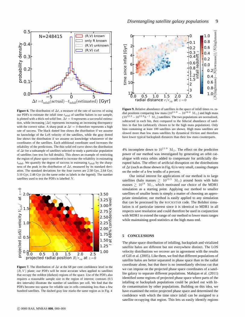
Figure 6. The distribution of∆t, a measure of the rate of success of usingour PDFs to estimate the infall timetinfall of satellite haloes in our sample,is plotted with a thick red solid line.∆t = 0 represents a successful estima-tion, while increasing|∆t| represents increasing an increasing discrepancywith the correct value. A sharp peak at∆t = 0 therefore represents a highrate of success. The black dotted line shows the distribution if we assumeno knowledge of the LoS velocity of the satellites, while thegray dottedline shows the distribution if we assume no knowledge whatsoever of thecoordinates of the satellites. Each additional coordinateused increases thereliability of the predictions. The thin solid red curve shows the distributionof ∆t for a subsample of satellites selected to study a particularpopulationof satellites (see text for full details). This shows an example of restrictingthe region of phase space considered to increase the reliability in estimatingtinfall . We quantify the degree of success in estimatingtinfall by the sharp-ness of the peak in the distribution of∆t, measured by its standard devi-ation. The standard deviations for the four curves are 2.58 Gyr, 2.64 Gyr,3.10 Gyr, 2.48 Gyr (in the same order as labels in the legend).The numbersatellites used to test the PDFs is labelledN .
0.0 0.5 1.0 1.5 2.0 2.5projected radial position R/rvir at z=0
0.0
0.5
1.0
1.5
2.0
projec
ted (LoS
) veloc
ity V
LoS/σ at z
=0
100
1000
1.001.251.501.752.002.252.502.753.003.253.50
∆t a
t 68%
con
fiden
ce le
vel
Figure 7. The distribution of∆t at the 68 per cent confidence level in the(R, V ) plane; our PDFs will be most accurate when applied to satellitesthat occupy the reddest (darkest) regions of the space. Use of the PDFs alsorequires a reasonable sample size in the region of interest;contours (0.5dex intervals) illustrate the number of satellites per cell. We find that thePDFs become too sparse for reliable use in cells containing less than a fewhundred satellites. The dashed gray line marks the same region as in Fig. 4
0.0 0.5 1.0 1.5 2.0 2.5radial distance r/rvir at z=0
12
10
8
6
4
2
0
time sinc
e infall [G
yr]
00.10.20.30.40.60.811.21.523
infall reds
hift z
−1.0−0.8−0.6−0.4−0.20.00.20.40.60.81.0
(N(highmass)−
N(lowmass))/N(highmass)
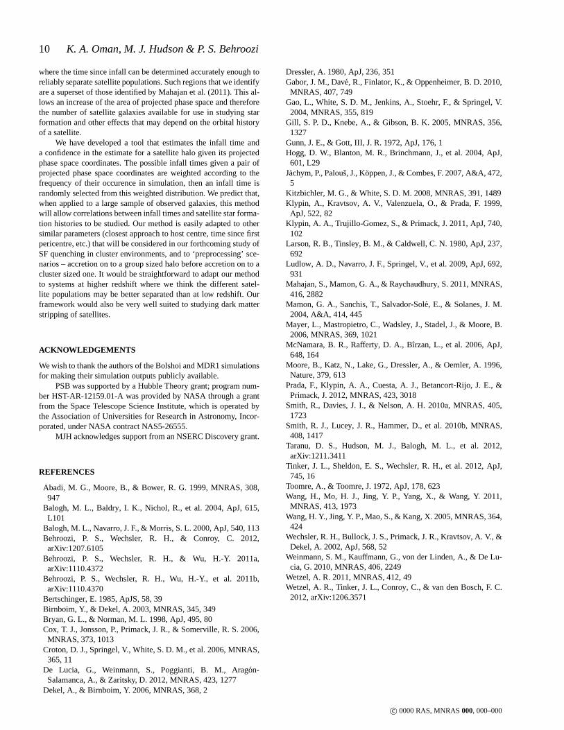
Figure 9. Relative abundance of satellites in the space of infall times vs. ra-dial positions comparing low mass (1011.9 − 1012.2 M⊙) and high mass(1012.2−1012.8h−1 M⊙) satellites. The two populations are normalized,subtracted in each bin, then compared to the fiducial abundance of satel-lites in that bin (arbitrarily chosen to be the high mass population). Onlybins containing at least 100 satellites are shown. High masssatellites areslowed more than low mass satellites by dynamical friction and thereforehave lower typical backsplash distances than their low masscounterparts.
4% incomplete down to1011.9 M⊙. The effect on the predictivepower of our method was investigated by generating an orbit cat-alogue with extra orbits added to compensate for artificially dis-rupted halos. The effect of artificial disruption on the distributionsof ∆t (such as those shown in Fig. 6) is very small, causing changeson the order of a few tenths of a percent.
Our initial interest for applications of our method is to largesatellites (halo masses& 1012.5 M⊙) around hosts with halomasses& 1014 M⊙, which motivated our choice of the MDR1simulation as a starting point. Applying our method to smallersatellites of smaller hosts is simply a matter of choosing anappro-priate simulation; our method is easily applied to any simulationthat can be processed by theROCKSTARcode. The Bolshoi simu-lation is of particular interest since it is identical to MDR1 in allrespects save resolution and could therefore be used in conjunctionwith MDR1 to extend the range of our method to lower mass rangeswhile maintaining good statistics at the high mass end.
5 CONCLUSIONS
The phase space distribution of infalling, backsplash and virializedsatellite halos are different but not everywhere distinct.The LOSvelocity distributions we recover are in agreement with theresultsof Gill et al. (2005). Like them, we find that different populations ofsatellite halos are better separated in phase space than in the radialcoordinate alone, but that there is no immediately obvious cut thatwe can impose on the projected phase space coordinates of a satel-lite galaxy to separate different populations. Mahajan et al. (2011)identified some regions of projected phase space where partsof theinfalling or backsplash populations could be picked out with lit-tle contamination by other populations. Building on this idea, wehave examined the entire projected phase space and determined theconfidence with which the time since infall can be assigned toasatellite occupying that region. This lets us easily identify regions
c© 0000 RAS, MNRAS000, 000–000
10 K. A. Oman, M. J. Hudson & P. S. Behroozi
where the time since infall can be determined accurately enough toreliably separate satellite populations. Such regions that we identifyare a superset of those identified by Mahajan et al. (2011). This al-lows an increase of the area of projected phase space and thereforethe number of satellite galaxies available for use in studying starformation and other effects that may depend on the orbital historyof a satellite.
We have developed a tool that estimates the infall time anda confidence in the estimate for a satellite halo given its projectedphase space coordinates. The possible infall times given a pair ofprojected phase space coordinates are weighted according to thefrequency of their occurence in simulation, then an infall time israndomly selected from this weighted distribution. We predict that,when applied to a large sample of observed galaxies, this methodwill allow correlations between infall times and satellitestar forma-tion histories to be studied. Our method is easily adapted toothersimilar parameters (closest approach to host centre, time since firstpericentre, etc.) that will be considered in our forthcoming study ofSF quenching in cluster environments, and to ‘preprocessing’ sce-narios – accretion on to a group sized halo before accretion on to acluster sized one. It would be straightforward to adapt our methodto systems at higher redshift where we think the different satel-lite populations may be better separated than at low redshift. Ourframework would also be very well suited to studying dark matterstripping of satellites.
ACKNOWLEDGEMENTS
We wish to thank the authors of the Bolshoi and MDR1 simulationsfor making their simulation outputs publicly available.
PSB was supported by a Hubble Theory grant; program num-ber HST-AR-12159.01-A was provided by NASA through a grantfrom the Space Telescope Science Institute, which is operated bythe Association of Universities for Research in Astronomy,Incor-porated, under NASA contract NAS5-26555.
MJH acknowledges support from an NSERC Discovery grant.
REFERENCES
Abadi, M. G., Moore, B., & Bower, R. G. 1999, MNRAS, 308,947
Balogh, M. L., Baldry, I. K., Nichol, R., et al. 2004, ApJ, 615,L101
Balogh, M. L., Navarro, J. F., & Morris, S. L. 2000, ApJ, 540, 113Behroozi, P. S., Wechsler, R. H., & Conroy, C. 2012,arXiv:1207.6105
Behroozi, P. S., Wechsler, R. H., & Wu, H.-Y. 2011a,arXiv:1110.4372
Behroozi, P. S., Wechsler, R. H., Wu, H.-Y., et al. 2011b,arXiv:1110.4370
Bertschinger, E. 1985, ApJS, 58, 39Birnboim, Y., & Dekel, A. 2003, MNRAS, 345, 349Bryan, G. L., & Norman, M. L. 1998, ApJ, 495, 80Cox, T. J., Jonsson, P., Primack, J. R., & Somerville, R. S. 2006,MNRAS, 373, 1013
Croton, D. J., Springel, V., White, S. D. M., et al. 2006, MNRAS,365, 11
De Lucia, G., Weinmann, S., Poggianti, B. M., Aragon-Salamanca, A., & Zaritsky, D. 2012, MNRAS, 423, 1277
Dekel, A., & Birnboim, Y. 2006, MNRAS, 368, 2
Dressler, A. 1980, ApJ, 236, 351Gabor, J. M., Dave, R., Finlator, K., & Oppenheimer, B. D. 2010,MNRAS, 407, 749
Gao, L., White, S. D. M., Jenkins, A., Stoehr, F., & Springel,V.2004, MNRAS, 355, 819
Gill, S. P. D., Knebe, A., & Gibson, B. K. 2005, MNRAS, 356,1327
Gunn, J. E., & Gott, III, J. R. 1972, ApJ, 176, 1Hogg, D. W., Blanton, M. R., Brinchmann, J., et al. 2004, ApJ,601, L29
Jachym, P., Palous, J., Koppen, J., & Combes, F. 2007, A&A, 472,5
Kitzbichler, M. G., & White, S. D. M. 2008, MNRAS, 391, 1489Klypin, A., Kravtsov, A. V., Valenzuela, O., & Prada, F. 1999,ApJ, 522, 82
Klypin, A. A., Trujillo-Gomez, S., & Primack, J. 2011, ApJ, 740,102
Larson, R. B., Tinsley, B. M., & Caldwell, C. N. 1980, ApJ, 237,692
Ludlow, A. D., Navarro, J. F., Springel, V., et al. 2009, ApJ,692,931
Mahajan, S., Mamon, G. A., & Raychaudhury, S. 2011, MNRAS,416, 2882
Mamon, G. A., Sanchis, T., Salvador-Sole, E., & Solanes, J.M.2004, A&A, 414, 445
Mayer, L., Mastropietro, C., Wadsley, J., Stadel, J., & Moore, B.2006, MNRAS, 369, 1021
McNamara, B. R., Rafferty, D. A., Bırzan, L., et al. 2006, ApJ,648, 164
Moore, B., Katz, N., Lake, G., Dressler, A., & Oemler, A. 1996,Nature, 379, 613
Prada, F., Klypin, A. A., Cuesta, A. J., Betancort-Rijo, J. E., &Primack, J. 2012, MNRAS, 423, 3018
Smith, R., Davies, J. I., & Nelson, A. H. 2010a, MNRAS, 405,1723
Smith, R. J., Lucey, J. R., Hammer, D., et al. 2010b, MNRAS,408, 1417
Taranu, D. S., Hudson, M. J., Balogh, M. L., et al. 2012,arXiv:1211.3411
Tinker, J. L., Sheldon, E. S., Wechsler, R. H., et al. 2012, ApJ,745, 16
Toomre, A., & Toomre, J. 1972, ApJ, 178, 623Wang, H., Mo, H. J., Jing, Y. P., Yang, X., & Wang, Y. 2011,MNRAS, 413, 1973
Wang, H. Y., Jing, Y. P., Mao, S., & Kang, X. 2005, MNRAS, 364,424
Wechsler, R. H., Bullock, J. S., Primack, J. R., Kravtsov, A.V., &Dekel, A. 2002, ApJ, 568, 52
Weinmann, S. M., Kauffmann, G., von der Linden, A., & De Lu-cia, G. 2010, MNRAS, 406, 2249
Wetzel, A. R. 2011, MNRAS, 412, 49Wetzel, A. R., Tinker, J. L., Conroy, C., & van den Bosch, F. C.2012, arXiv:1206.3571
c© 0000 RAS, MNRAS000, 000–000