DISI - University of Trento Approximate Explicit MPC and …eprints-phd.biblio.unitn.it/823/1/PhD-Thesis-Trimboli.pdf · · 2012-12-02PhD Dissertation International ... cial PWA

PhD Dissertation

International Doctorate School in Information andCommunication Technologies

DISI - University of Trento

Approximate Explicit MPC and Closed-loop StabilityAnalysis based on PWA Lyapunov Functions

Sergio Trimboli

Advisor:

Prof. Alberto Bemporad

IMT Institute for Advanced Studies Lucca

XXV Cycle - November 2012

Abstract

Model Predictive Control (MPC) is the de facto standard in advanced industrial

automation systems. There are two main formulations of the MPC algorithm:

an implicit one and an explicit MPC one. The first requires an optimization

problem to be solved on-line, which is the main limitation when dealing with

hard real-time applications. As the implicit MPC algorithm cannot be guaran-

teed in terms of execution time, in many applications the explicit MPC solution

is preferable. In order to deal with systems integrating mixed logic and dynam-

ics, the class of the hybrid and piecewise affine models (PWA) were introduced

and tackled by the explicit MPC strategy. However, the resulting controller

complexity leads to a requirement on the CPU/memory combination which is as

strict as the number of states, inputs and outputs increases. To reduce drasti-

cally the complexity of the explicit controller while preserving the controller’s

performance, a strategy combining switched MPC with discontinuous simpli-

cial PWA models is introduced in this thesis. The latter is proven to be circuit

implementable, e.g., in FPGA. To ensure that closed-loop stability properties

are guaranteed, a stability analysis tool is proposed which exploits suitable and

possibly discontinuous PWA Lyapunov-like functions. The tool requires solving

offline a linear programming problem. Moreover, the tool is able to compute an

invariant set for the closed-loop system, as well as ultimate boundedness and

input-to-state stability properties.

Acknowledgements

This thesis is the result of three years of intense research partially supported bythe European Commission through project MOBY-DIC “Model-based synthesisof digital electronic circuits for embedded control” (FP7-INFSO-ICT-248858).I would like to express here the pleasure I had in working together with Prof.Alberto Bemporad. He gave me the possibility to gain a lot of experience inadvanced control topics. Alberto, I would like to thank you for sharing yourknowledge with me. This thesis, but more important the work possibilities Ihad, would never happen without your support.Also, I am grateful to all my co-authors for collaborating in a very productiveway. Stefano, Ilya, Matteo, Daniele, Marco, Tomaso, thank you for all the timeand knowledge we shared together.I would particularly like to extend warm thanks to the Committee of this thesis,Marco Storace, Mircea Lazar, Francesco Biral and Thorsten Hestermeyer.Special thanks are for Matteo. Without his guidance and experience, most ofthis thesis would be never carried out. Matteo, thank you for sharing yourmethodology and professional abilities. I would also thank you, my friend,for supporting me during my blackout together with Antonio and Laura.Antonio, your infinite patience and your infinite respect are the abilities that Irecognize the most in you. Thank you for all your support, my friend.

5

Mattia, Giuseppe, Claudio, Laura, Daniele, Carlo, Sara, Irena, thank you forvaluable friendship during the years in Trento. I would not spend too manywords to explain that I found friends in you. I would only say thank you guys.Davide, Simone, Daniele, Emiliano, Alessandro, Sara, Giulio, Ilaria, Rudy,Fabio, Alfio, Stefano thank you for the time we spent together during my firststudies in Siena. Thank you for introducing me in the real Ph.D. lifestyle.Finally, I would like to thank my family for the immense support I received inthose years (and still now). Antonio and Tina, I am very lucky and I am gladto be your son. This thesis and this Ph.D. is the result of the freedom I hadin choosing my way, since of your sacrifices and my effort. I wish to thankGiuliarosa and Walter for their advices and insight. Thank you, with love.

i

ii

Contents

1 Introduction 11.1 The problem . . . . . . . . . . . . . . . . . . . . . . . . . . . . 3

1.2 Contribution . . . . . . . . . . . . . . . . . . . . . . . . . . . . 4

1.3 Summary of publications . . . . . . . . . . . . . . . . . . . . . 5

1.4 Structure of the Thesis . . . . . . . . . . . . . . . . . . . . . . 6

1.5 Basic notations and definitions . . . . . . . . . . . . . . . . . . 7

2 State of the Art 92.1 Framework . . . . . . . . . . . . . . . . . . . . . . . . . . . . 9

2.1.1 MPC algorithm . . . . . . . . . . . . . . . . . . . . . . 9

2.1.2 Hybrid models . . . . . . . . . . . . . . . . . . . . . . 12

2.1.3 Explicit MPC . . . . . . . . . . . . . . . . . . . . . . . 13

2.1.4 Switched MPC . . . . . . . . . . . . . . . . . . . . . . 15

2.2 Controller circuit implementation . . . . . . . . . . . . . . . . . 15

2.3 Stability analysis . . . . . . . . . . . . . . . . . . . . . . . . . 17

3 Explicit HMPC approximation and FPGA implementation 213.1 Circuit implementation of continuous PWAS functions . . . . . 22

3.2 Generalization to a class of discontinuous functions . . . . . . . 24

iii

3.2.1 An example . . . . . . . . . . . . . . . . . . . . . . . . 283.3 Switched MPC . . . . . . . . . . . . . . . . . . . . . . . . . . 303.4 Experimental validation . . . . . . . . . . . . . . . . . . . . . . 33

3.4.1 Model and control description . . . . . . . . . . . . . . 343.4.2 FPGA implementation . . . . . . . . . . . . . . . . . . 35

4 Closed-loop stability analysis 414.1 Problem formulation . . . . . . . . . . . . . . . . . . . . . . . 424.2 Reachability analysis . . . . . . . . . . . . . . . . . . . . . . . 44

4.2.1 One-step reachability analysis . . . . . . . . . . . . . . 444.2.2 Fake dynamics and extended system . . . . . . . . . . . 454.2.3 Case of additive disturbances only . . . . . . . . . . . . 46

4.3 PWA Lyapunov analysis for the extended system . . . . . . . . 484.3.1 Asymptotic stability . . . . . . . . . . . . . . . . . . . 484.3.2 Ultimate boundedness . . . . . . . . . . . . . . . . . . 534.3.3 Feasibility issues . . . . . . . . . . . . . . . . . . . . . 60

4.4 Invariance analysis . . . . . . . . . . . . . . . . . . . . . . . . 614.5 Input-to-State Stability . . . . . . . . . . . . . . . . . . . . . . 634.6 Simulation examples . . . . . . . . . . . . . . . . . . . . . . . 66

4.6.1 Uniform asymptotic stability . . . . . . . . . . . . . . . 684.6.2 Uniform ultimate boundedness . . . . . . . . . . . . . . 724.6.3 Input-to-state stability . . . . . . . . . . . . . . . . . . 72

5 Conclusion 77

Bibliography 81

iv

List of Tables

3.1 Number of elementary devices to evaluate a discontinuous PWAS 293.2 Controllers dimensions . . . . . . . . . . . . . . . . . . . . . . 38

v

List of Figures

2.1 Implicit MPC algorithm . . . . . . . . . . . . . . . . . . . . . . 10

3.1 Two-dimensional domain with discontinuities. . . . . . . . . . . 253.2 One-dimensional discontinuous PWAS function . . . . . . . . . 273.3 Architecture to implement discontinuous functions . . . . . . . 293.4 PWA state partitions for u = 25C. . . . . . . . . . . . . . . . . 363.5 Differences between manipulated variables of HMPC and SwMPC

for ry = 30. . . . . . . . . . . . . . . . . . . . . . . . . . . . . 373.6 HMPC (blue) vs. PWAS (black). . . . . . . . . . . . . . . . . . 39

4.1 The invariant set XH for case A is constituted by the union ofthe regions of the explicit MPC and the box XH \ X (the greyrectangle on the left) . . . . . . . . . . . . . . . . . . . . . . . 69

4.2 The PWA Lyapunov function for the extended system in case A 704.3 The invariant set P obtained in case A . . . . . . . . . . . . . . 714.4 The PWA Lyapunov-like function for the extended system in

case B . . . . . . . . . . . . . . . . . . . . . . . . . . . . . . . 734.5 The invariant set P and the terminal set F (shaded) in case B . . 744.6 The sets P ≡ X andR(P)⊕B∞2 (in black) in case C . . . . . 76

vii

Chapter 1

Introduction

During the last decades Model Predictive Control (MPC) has become the mostused technology in highly automated industry [4]. Right now MPC is a stan-dard control approach for both large and medium/small scale processes, evenif they are highly complex and multivariable. The word model in the acronymMPC stands for model-based, while the word predictive means that there is aso-called prediction of the future behavior of the process when selecting thecontrol action.MPC exploits the knowledge of a dynamical model that describes the plant be-havior in the time domain (usually a state-space model), and is based on an opti-mization problem that minimizes a cost function, usually leading to a quadraticprogramming problem. Due to physical reasons, the plant actuators are oftenconstrained to operate in a certain range and this implies the imposition of con-straints in the optimization algorithm associated with the MPC control law. Itis clear that the constraints on the state, input and output of a dynamical systemare embedded in the MPC algorithm and are not imposed a posteriori, as occursin classical control theory (e.g., PID controllers).One basic block of MPC strategy is the state-space mathematical model. The

1

2

interactions between the state variables are described by a set of differentialor difference equations, for continuous-time and discrete-time models, respec-tively. In general, the simpler is the model in terms of number of states, thebetter it is for MPC design.There exist two main formulations for MPC, the implicit MPC and the explicit

MPC. If the system is linear with linear constraints (or can be approximatedby such a system), one can map the implicit MPC formulation to an equivalentexplicit MPC formulation. By solving an off-line multi-parametric linear orquadratic optimization problem (mpLP, mpQP), the implicit controller can bemapped to a piecewise affine (PWA) explicit control law, that can be evaluatedon-line rather easily [1].The on-line computational complexity of the explicit MPC algorithm can be es-timated exactly. The complexity of the off-line multi-parametric optimizationproblem grows very quickly with respect to the number of constraints in theMPC problem. As a result, for a very large scale problem, the implicit MPCstrategy may be the only viable solution.Technological innovation drives the attention to a class of models that can dealwith continuous and discrete components of systems. The dynamical modelexploited in the MPC technology can integrate logical rules, switching physicallaws and different kind of operating constraints. As a matter of fact, the hybrid

system class of dynamical models integrating logical behavior has been devel-oped [7].The term hybrid system was introduced to describe the combination of con-tinuous dynamical and discrete event systems. The hybrid models can dealwith implicit and explicit MPC strategy, as the logical rules for that model canbe translated in constraints for the optimization problem, at the expense of its

3 CHAPTER 1. INTRODUCTION

complexity. The closed-loop stability and optimality analysis are only two ofthe currently open problems in the MPC research community. Many are themilestone papers, for instance [30], in which the researchers undertake the sta-bility and the optimality issues. Also the MPC robustness problem is addressedin [8], in which the authors survey the possible presence of uncertainty in the dy-namical model description together with the stability and performance issues.The aim of this thesis is to develop low complexity solutions for the controlproblem based on an MPC strategy, even if the model is hybrid, with partic-ular attention to real-time implementation issues. This involves the stabilityproblem, that must be solved. The stability results will provide the theoreti-cal background for low complexity MPC solutions in the hybrid explicit MPCframework.

1.1 The problem

For time-critical applications the implicit MPC solution is not suitable, hencethe explicit solution is more compatible. In the explicit MPC strategy, the fea-sible set of the multi-parametric optimization problem is bounded and the dy-namics are continuous function in that set. The assumption of a bounded set isnot restrictive when it is coupled with real life applications issues.If the system under control is not only described by differential or differenceequations, but integrates a switching dynamics logic, then the model can bestated as hybrid model. A particular class of hybrid models is the PWA de-scription, that is suitable for representing a switching system or a region-wiselinearized system. An explicit MPC of a PWA system results typically in a very

1.2. CONTRIBUTION 4

complex multi-parametric optimization problem. The implementation of the re-sulting explicit PWA control law, assuming one is able to determine it offline,in the closed-loop can be very hard, due to the large number of regions (i.e. thelookup table is hard to store and to search).The main problem is that the explicit MPC solution is employed when the sam-ple time must be small, but for large controller (i.e. too many regions) this leadsto an inapplicable solution. As a result of the analysis of the state of the artin the hard real time control framework, the target of this thesis is the studyof low complexity solution for explicit MPC of PWA systems (e.g., switchingMPC), by also addressing the closed-loop stability problem for this class ofsystems. Moreover, the synthesized low complexity controller can be circuitimplementable, thus leading to a complete bundle that fulfills the requirementson sampling time, circuit architecture, controller performances and closed loop-stability.Right now, the literature results on explicit MPC stability are not directly appli-cable to low complexity solutions. For instance, if the low complexity controlleris the result of a union of several PWA laws (i.e. switching MPC), right nowthere are few and patchy results giving a stability region in which the controllerwill be stabilizing for the closed loop, even if the switching MPC can be rep-resented as a PWA control law (i.e. union of PWA). In this case, the stability

analysis problem is addressed in this thesis.

1.2 Contribution

First of all, in this thesis we introduce a digital architecture implementing theexplicit solution of a switched MPC problem. Given a mixed-logic dynamical


system, we derive an explicit controller in the form of a possibly discontinuouspiecewise-affine function. This function is then approximated by resorting topiecewise-affine simplicial functions, which can be implemented on a circuitby extending the representation capabilities of a previously proposed architec-ture to evaluate the control action. The architecture has been implemented onFPGA and validated on a benchmark example related to an air conditioning sys-tem.Secondarily, this thesis proposes a method to analyze uniform asymptotic sta-bility, uniform ultimate boundedness, and input-to-state stability of uncertainpiecewise affine systems whose dynamics are only defined in a bounded andpossibly non-invariant set X of states. The approach relies on introducing fakedynamics outside X and on synthesizing a piecewise affine and possibly dis-continuous Lyapunov function via linear programming. The existence of such afunction proves stability properties of the original system and allows the deter-mination of a region of attraction contained in X . The procedure is particularlyuseful in practical applications for analyzing the stability of piecewise affinecontrol systems that are only defined over a bounded subsetX of the state space,and to determine whether for a given set of initial conditions the trajectories ofthe state vector remain within the domain X .

1.3 Summary of publications

This thesis is based on the following publications.

• S. Trimboli, M. Rubagotti and A. Bemporad, Stability and invariance anal-ysis of uncertain PWA systems based on linear programming, in 50th IEEECDC-ECC, Orlando, FL, USA, 2011.

1.4. STRUCTURE OF THE THESIS 6

• M. Rubagotti, S. Trimboli, D. Bernardini and A. Bemporad, Stability andinvariance analysis of approximate explicit MPC based on PWA Lyapunovfunctions, in 18th IFAC World Congress, Milano, Italy, 2011.

• T. Poggi, S. Trimboli, A. Bemporad and M. Storace, Explicit hybrid modelpredictive control: discontinuous piecewise-affine approximation and FPGAimplementation, in 18th IFAC World Congress, Milano, Italy, 2011.

1.4 Structure of the Thesis

This thesis is organized as follows. After a first introduction of the problemand the contribution, given in Chapter 1, some preliminary concepts are in-troduced in Section 1.5. In Chapter 2 is given the general MPC frameworkin which this thesis is contextualized, as well as the state of the art of circuitimplementation of PWA controllers and the related stability analysis problem.In Section 3, the architecture for the electronic implementation of discontinu-ous PWAS functions is introduced. Then the architecture is used to implementexplicit switched MPC controllers. The procedure is tested on a hybrid tem-perature control system. Both the maximum working frequency and the powerconsumption of the control FPGA implementation are estimated in the rangeof tens of MHz and tens of mW, respectively. The closed-loop stability anal-ysis problem is addressed in Chapter 4. 4.1 introduces the class of considereduncertain PWA systems. 4.2 is devoted to the one-step reachability analysis ofthe system, while the main results on the analysis of the extended system areformulated in 4.3. The region of attraction is obtained in Section 4.4, wherethe analysis of the original system is performed. The input-to-state stability ofthe system is analyzed in 4.5. 4.6 shows simulation examples. Conclusions are


gathered in Chapter 5.

1.5 Basic notations and definitions

Let R, R+, Z and Z+ denote the sets of reals, non-negative reals, integers andnon-negative integers, respectively. The floor function b·c of a ∈ R is definedas the largest b ∈ Z such that a ≥ b. The symbol ‖ · ‖ represent any p-norm ofa vector, while ‖ · ‖∞ represents the infinity norm. With respect to the infinitynorm, we define the norm ball of radius χ > 0 as B∞χ , a ∈ Rn : ‖a‖∞ ≤ χ.Given a discrete-time signal v : Z+ → Rnv , the sequence of the values of v fromthe zero instant to the k-th instant is denoted by v[k]. The norm of a sequenceis defined as ‖v[k]‖ , sup‖v(i)‖, for i = 1, ..., k. Given a set A ⊆ Rn, itsinterior is denoted by int(A), its closure by A, and its convex hull by conv(A).If A is a polyhedron, the set of the vertices of A is denoted by vert(A). Abounded polyhedron is called polytope. Given two sets A ∈ Rn and B ∈ Rn,the Minkowski sum is A ⊕ B , a + b : a ∈ A, b ∈ B. A function γ :

R+ → R+ is called K-function if it is continuous, positive definite, and strictlyincreasing. A function φ : R+ × Z+ → R+ is a KL-function if, for each fixedk ≥ 0, φ(·, k) is a K function, for each fixed c ≥ 0, φ(c, ·) is decreasing, andφ(c, k)→ 0 as t→∞.

Consider a generic discrete-time nonlinear system

x(k + 1) = f(x(k), v(k)) (1.1)

where x ∈ Rn is the state vector, the input v ∈ V ⊂ Rnv collects the modeluncertainties and external disturbances, and V is a compact set.

1.5. BASIC NOTATIONS AND DEFINITIONS 8

Definition 1 (One-step reachable set). Given a set X ⊂ Rn and system dynam-

ics (1.1), the one step reachable set from X is

R(X ) , y ∈ Rn : y = f(x, v), v ∈ V , x ∈ X

Definition 2 (RPI set). A set F ⊂ Rn is called robustly positively invariant(RPI) with respect to dynamics (1.1) if, for all x ∈ F and all v ∈ V , f(x, v) ∈F .

Definition 3 (Uniform asymptotic stability). Given a set X ⊆ Rn with 0 ∈ X ,

system (1.1) is uniformly asymptotically stable in X (UAS(X )) if there exists

a KL-function φ such that, for all the initial conditions x(0) ∈ X and for all

the sequences v[k] with v(i) ∈ V , i = 0, ..., k, ‖x(k)‖ ≤ φ(‖x(0)‖, k), for all

k ∈ Z+.

Definition 4 (Uniform ultimate boundedness). Given a set X ⊆ Rn and an RPI

set F ⊆ X , with 0 ∈ int(F), system (1.1) is uniformly ultimately bounded from

X to F (UUB(X ,F)) if, for all a > 0 there exist T (a) > 0 such that, for every

x(0) ∈ X with ‖x(0)‖ ≤ a, x(T ) ∈ F for all the sequences v[k] with v(i) ∈ V ,

i = 0, ..., k.

Definition 5 (Input-to-state stability). Given a set X ⊆ Rn with 0 ∈ X , system

(1.1) is input-to-state stable in X (ISS(X )) if there exist a KL-function φ and

a K-function γ such that, for all the initial conditions x(0) ∈ X and for all the

sequences v[k] with v(i) ∈ V , i = 0, ..., k, ‖x(k)‖ ≤ φ(‖x(0)‖, k)+γ(‖v[k−1]‖),

for all k ∈ Z+.

Chapter 2

State of the Art

2.1 Framework

2.1.1 MPC algorithm

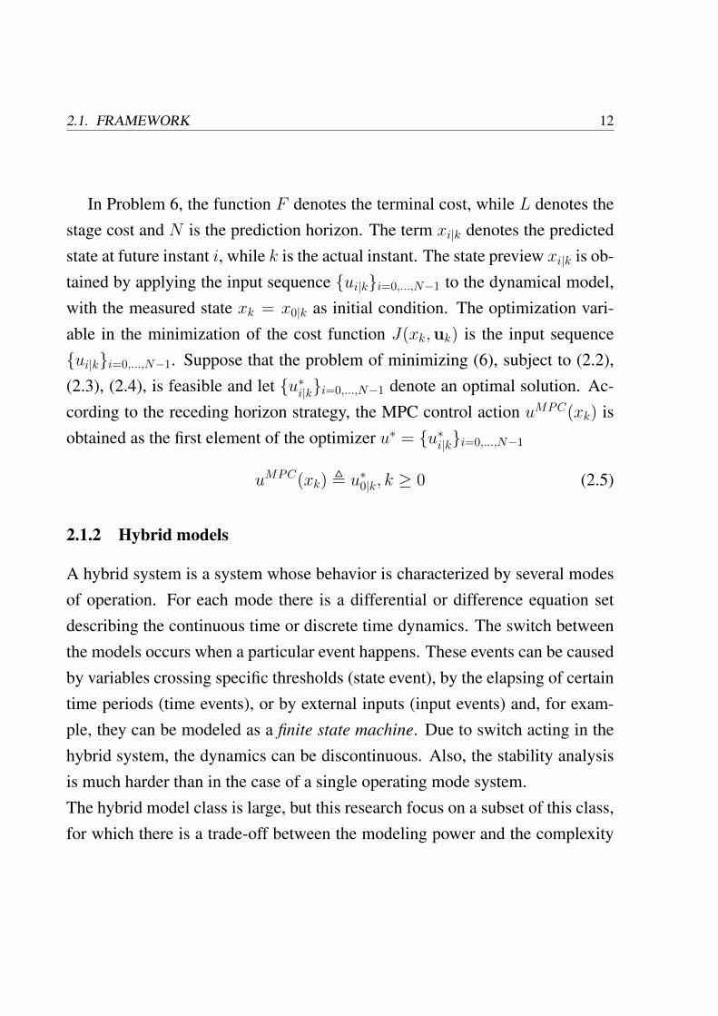
The use of a prediction model, the use of an optimization problem subject toconstraints and the receding horizon strategy are the three key principles forstating the MPC algorithm. The control algorithm involves the evaluation ofan on-line and open-loop optimization subject to state, input and output con-straints, in which the prediction model is incorporated. Since only the firstinput of the optimal sequence is applied, the MPC methodology is also calledreceding horizon.Referring to Figure 2.1, an instant detailed description of the implicit MPC algo-rithm is given. At each discrete-time t, the measurements yt acquired from thesensors and the dynamical model are used in order to predict the plant behavior.The state prediction is computed among a N -step time window (N is usuallycalled prediction horizon). The optimal input sequence u∗t+k is computed byminimizing the related cost function. According to the receding horizon con-trol paradigm, only the first element of the optimal sequence u∗ is applied as the

9

2.1. FRAMEWORK 10

minN−1

k=0

Wy(yt+k − r(t))2 + W∆u∆ut+k2

s.t. xt+k+1 = Axt+k + But+k

yt+k = Cxt+k + Dut+k

∆ut+k = ut+k − ut+k−1

umin ≤ ut+k ≤ umax

∆umin ≤ ∆ut+k ≤ ∆umax

ymin ≤ yt+k ≤ ymax

xt = x(t), k = 0, . . . , N − 1

!"#$%&'#'%()%*+%,-./0123

E5;-21%:4F%2<@0157G.

#

!"#$%&"'((%&")*+",-.)"/()01'%"1/2+"u*(t)

41-3567-3%087/879

:2;5/8<27-3=;/879

t t># t>N

ut>k

r3t4

t># t>& t>N>#

!"!"#"$%&#t'()"5+)"$+6"1+'.7-+1+$).8"-+(+')")*+"/()0109')0/$:";$<"./"/$"="""""

%*3?2;72@-%0A%1-/-27-3%0;B<5;-%0/75.5C2750;D%*++,-!./0

yt>k

!"!"#"$%& t)"./%2+"'$"12"$%34#516"714"(-/>%+1"/2+-"'"?7)7-+"*/-09/$"/? N .)+(.

@*0."0."'"893:73"$5#271;73%%$6;#<=>?(-/>%+1"60)*"-+.(+A)")/")*+".+B7+$A+/?"0$(7)"0$A-+1+$)."Cut8"=8"Cut+N-1

venerdì 7 gennaio 2011

Figure 2.1: Implicit MPC algorithm

11 CHAPTER 2. STATE OF THE ART

input ut+1 of the real plant. At the next time step t+1, a new optimization prob-lem is solved by exploiting the new measurements, and only the first elementof the resulting optimal control sequence is applied to the plant. As a result ofthe receding horizon strategy, it follows that the control action is applied in aclosed-loop fashion.In general the dynamical model can be nonlinear, the cost function can be a 2-norm, 1-norm or∞-norm and the constraints can be time varying. A nonlineardynamical system implies a more complicated optimization algorithm. For a 1-norm or a∞-norm cost function is sufficient a linear programming algorithm,while for a 2-norm cost function is required a quadratic programming algorithm.Moreover, time varying constraints imply a high computational burden. In thefollowing, a general formulation of MPC problem is stated.

Definition 6 (Problem). Let N ≥ 1 be given, let X ⊆ Rn and U ⊆ Rm be sets

which represent the state and the input constraints, respectively, and contain

the origin in their interior. The prediction model is xk+1 = g(xk, uk), k ≥ 0,

with g : Rn × Rm → Rn a nonlinear, possibly discontinuous function with

g(0, 0) = 0. Let F : Rn → R+ with F (0) = 0 and L : Rn × Rm → R+ with

L(0, 0) = 0 be known mappings. For each discrete time instant k ≥ 0 let xk the

measured state, let x0|k , xk and minimize the cost function

J(xk,uk) , F (xN |k) +N−1∑

i=0

L(xi|k, ui|k) (2.1)

over all input sequences uk , (u0|k, . . . , uN−1|k) subject to the constraints

xi+1|k , g(xi+1|k, ui|k) , i = 0, . . . , N − 1, (2.2)

xi+1|k ∈ X , ∀i = 1, . . . , N, (2.3)

ui|k ∈ U , ∀i = 1, . . . , N − 1 (2.4)

2.1. FRAMEWORK 12

In Problem 6, the function F denotes the terminal cost, while L denotes thestage cost and N is the prediction horizon. The term xi|k denotes the predictedstate at future instant i, while k is the actual instant. The state preview xi|k is ob-tained by applying the input sequence ui|ki=0,...,N−1 to the dynamical model,with the measured state xk = x0|k as initial condition. The optimization vari-able in the minimization of the cost function J(xk,uk) is the input sequenceui|ki=0,...,N−1. Suppose that the problem of minimizing (6), subject to (2.2),(2.3), (2.4), is feasible and let u∗i|ki=0,...,N−1 denote an optimal solution. Ac-cording to the receding horizon strategy, the MPC control action uMPC(xk) isobtained as the first element of the optimizer u∗ = u∗i|ki=0,...,N−1

uMPC(xk) , u∗0|k, k ≥ 0 (2.5)

2.1.2 Hybrid models

A hybrid system is a system whose behavior is characterized by several modesof operation. For each mode there is a differential or difference equation setdescribing the continuous time or discrete time dynamics. The switch betweenthe models occurs when a particular event happens. These events can be causedby variables crossing specific thresholds (state event), by the elapsing of certaintime periods (time events), or by external inputs (input events) and, for exam-ple, they can be modeled as a finite state machine. Due to switch acting in thehybrid system, the dynamics can be discontinuous. Also, the stability analysisis much harder than in the case of a single operating mode system.The hybrid model class is large, but this research focus on a subset of this class,for which there is a trade-off between the modeling power and the complexity


of analysis. The trade-off results in a simpler model representation, but suffi-ciently structured in order to represent a industrially relevant process. Withoutloss of generality, in this paper the author considers the piecewise affine (PWA)functions as the class of hybrid models, defined as follows

Definition 7 (PWA Function). A function z(x) : X → Rs, where X ⊆ Rn is

a polyhedral set, is PWA if it is possible to partition X into convex polyhedral

regions, CRi, and z(x) = H ix+ ki, ∀x ∈ CRi.

In particular, a PWA model is described by the following definition

Definition 8 (PWA Model). A PWA dynamical model is the set of discrete time

linear systems

x(k + 1) = Aix(k) +Biu(k) + fi

y(k) = Cix(k) +Diu(k) + gi

i : Hix(k) + Liu(k) ≤ Ki, i = 1, . . . , s (2.6)

where Ai ∈ Rn×n, Bi ∈ Rn×m, Ci ∈ Rp×n, Di ∈ Rp×m, fi ∈ Rn, gi ∈ Rp are

the state space affine models, i is the active mode at time k and Hi, Li, Ki are

matrices of appropriate dimension.

In the Definition 8, for each i, the polytopic set depends on the state x(k)

and the input u(k) of the system. All the sets are polytopic, hence bounded bydefinition.

2.1.3 Explicit MPC

The implicit MPC strategy described in Section 2.1.1 requires to solve an on-line optimization problem. The corresponding code implementation of the al-

2.1. FRAMEWORK 14

gorithm is time unpredictable, hence it is not suitable for hard real-time imple-mentation, as it does not provide guarantees on the execution time. There area lot of processes for which implicit MPC is suitable, for instance a low fre-quency chemical plant, for which the execution time is not really important. Ahard real-time control loop must be time predictable, certifiable (i.e. providesguarantee) and relatively fast. However, the effort of the researchers in the fieldof the optimization algorithms has produced solutions to speed-up the optimiza-tion algorithm, for example the very fast active set strategies [21]. One of themost important result in the hard real-time control is addressed in the explicitsolution of the implicit MPC strategy [5].The idea behind the explicit MPC is to solve off-line several implicit MPC in-stances for all xk within a given set X = x ∈ Rn : Hx ≤ K ⊂ Rn, and tomake the dependence of the input on the state explicit. The set X is assumed tobe polytopic (i.e. bounded set and described by linear inequalities). As a result,by solving a multi-parametric program, the equivalent explicit solution of theimplicit ones is a piecewise affine function of the state

u(k) = F ix(k) +Gi

if H ix(k) ≤ K i (2.7)

where i indexes the i-th regionR in the explicit linear MPC.Also, for a hybrid model, under the assumption of bounded state and linear costfunction, the explicit MPC solution is a PWA function of the state.It is clear that formulation (2.6) is more suitable for real-time controllers, ratherthan the solution of implicit MPC. In order to evaluate the optimal input at timestep k, one has to evaluate a finite number of sets of inequalities and has to com-pute one matrix product and one sum. The actual microprocessor technology issufficiently mature to achieve that specifications. As the resulting few lines of


code can run in high speed, the explicit MPC is suitable for time-critical appli-cations.

2.1.4 Switched MPC

The architecture described in the previous sections can be used to implement anexplicit SwMPC controller in approximate form. In this section we summarizethe main elements of the SwMPC control strategy. A MLD system subject toconstraints can be controlled through an implicit HMPC strategy. The explicitHMPC strategy can be applied to a MLD model, after recasting it to an equiv-alent PWA form. A suitable strategy to control (2.6) in state feedback, subjectto state and input constraints, is the explicit HMPC [2]. This approach requiresenumerating all the feasible switch sequences between the dynamics i and solv-ing a multi-parametric quadratic problem for each sequence. Storing all thecontrol gains leads to a large use of memory blocks in the FPGA implementa-tion with respect to a simpler controller such as the SwMPC. Considering onlythe sequences for which the region i is the same during the prediction steps,since the constraints that define the PWA regions are ignored after the first pre-diction step, the number of multi-parametric quadratic problems to be solvedis equal to the number of PWA regions, leading to a suboptimal solution to thecontrol problem. A formal definition of the SwMPC will be given in Sec. 3.3.

2.2 Controller circuit implementation

The real-time implementation of linear model predictive control strategies inembedded architectures was deeply analyzed in [13,29], and an automated code

2.2. CONTROLLER CIRCUIT IMPLEMENTATION 16

generation strategy was developed in [36]. Starting from a model, through thedefinition of a model-based control strategy suitable for the implementation inan embedded architecture, the problem of implementing the control strategywas also investigated for parallel architectures in [28]. Often a system that inte-grates continuous dynamics and logical structures can be described as a mixed-logic dynamical system (MLD). A suitable strategy to control a MLD systemsubject to constraints is hybrid model predictive control (HMPC). In order toobtain a HMPC, one has to solve on-line a mixed-integer quadratic or a mixed-integer linear programming problem. For a high-dimensional model, solvingthis kind of problems may be computationally too expensive for fast real-timeapplication [14].

Explicit reformulations of HMPC can be carried out by solving off-line asequence of multi-parametric quadratic or linear problems [14]. The result-ing solution is a possibly discontinuous piecewise affine (PWA) function ofthe state. In other words, the control modes are linear affine over polytopespartitioning the state domain, thus making this approach more suitable for theembedded control implementations. Storing the gains of the explicit HMPC re-quires larger and larger memory blocks in the electronic implementation as thenumber of partitions grows. Moreover, in order to evaluate the control action,the pre-computed gains should be selected, according to the state value, from alook-up table associated to the explicit controller. As a result, since the gainsselection from the look-up table can be made by a binary-tree search [41], orby other more sophisticated algorithms, determining the correct mode can be ahard problem if the number of regions is too large.

A suitable strategy, alternative to HMPC, to reduce drastically the numberof partitions is the switched MPC (SwMPC) approach, successfully applied for


instance in [18], where a PWA system is controlled by a set of linear MPCcontrollers, each one defined over a different polytope of the domain. In explicitform, SwMPC is basically a set of patched PWA controllers. For each i-thregion Ri of the domain, a linear MPC problem is solved, whose solution is acontinuous PWA function defined over a polytopic partition of the region. Notethat a MLD model can be converted in an equivalent PWA formulation [2].

The resulting PWA control function may be discontinuous only at the bound-aries of the regions. The overall number of polytopes obtained with the ex-plicit SwMPC approach is typically much lower than the one obtained with theexplicit HMPC, especially when the number of optimization variables grows.However, the SwMPC complexity reduction with respect to HMPC is not cost-less, since optimal switching sequences are restricted to constant mode se-quences, possibly breaking a-priori stability properties. However, a-posteriori

stability analysis of the SwMPC can be performed exploiting the results in [20]and in [38].

2.3 Stability analysis

In the last decade the interest in studying the dynamical properties of piece-wise affine (PWA) systems has increased considerably, due to their powerfulmodeling capabilities. Discrete-time PWA models are a special class of hybridsystems that can represent combinations of finite automata and linear dynam-ics, are a good approximation of nonlinear systems [39], and are equivalent tohybrid systems in mixed logical dynamical form [2, 7].

Analyzing the stability of PWA systems is fundamental to describe the prop-erties of an autonomous hybrid system, or to check a-posteriori the stability

2.3. STABILITY ANALYSIS 18

of a given closed-loop system [6, 17]. In particular, stability analysis becomesfundamental when a PWA control law is synthesized without a-priori guaran-tees of closed-loop stability, for example when explicit model predictive control(MPC) laws [9] are approximated in order to reduce their complexity [1].

The most widely used methods for stability analysis of discrete-time PWAsystems are based on piecewise quadratic (PWQ) Lyapunov functions [20].Such methods rely on the solution of a semi-definite program to get a stabil-ity certificate. As highlighted in [22], the search for a PWQ Lyapunov functioncan be overly conservative, even with the use of the so-called S-procedure (seee.g. [15]). A valid alternative are PWA Lyapunov functions, that are computedby solving a linear program (LP) [11]. Other types of Lyapunov functions canbe used for the same purpose, such as piecewise polynomial Lyapunov func-tions [34]. For an overview of such methods, the interested reader is referredto [11].

Most of the existing literature on stability analysis of PWA systems assumesthat the set X of states in which the PWA dynamics are defined is invariant, asthe notion of stability has no practical relevance if the state trajectory exits thedomain of definition of the dynamics [11]. However, often the PWA system tobe analyzed is defined in a set X that may not be invariant. A possible approachis to perform a reachability analysis to find the maximum positively invariantset to establish, using a recursive procedure, an invariant subset of the given setX (see [35], [12, Chap. 4-5] and the references therein). Unfortunately thisprocedure often leads to very involved solutions, due to the exponential com-plexity of reachability analysis of PWA systems, and in many cases searchingthe maximum invariant set is an undecidable problem.

Most of the existing literature on stability analysis of PWA systems also deals


with nominal stability analysis, in spite of the practical relevance in applicationsof certifying stability properties in the presence of disturbances. The problemconsists of determining if the state will converge to the origin (or to a termi-nal set) despite parametric uncertainties and/or external disturbances affectingthe process. The reason why this problem was almost ignored in the literatureis mostly due to the complexity of uncertain switching systems. Notably, in-teresting results were introduced for the case of additive disturbances in [24],where an optimal control strategy is synthesized to steer the state in finite timeto a terminal set, and in [35], where the authors determine how to drive thestate into the maximal robust invariant set in minimum time, using set-theoretictechniques. Some classical results appeared for parametric uncertainties in caseof linear parameter varying systems [12, Chap. 7]. Results for linear switchedsystems can be found in [45], where quadratic stabilizability is analyzed in caseof two discrete states and polytopic parametric uncertainties, and in [27], wherethe synthesis of switching control laws is tackled, assuring that the state is ul-timately bounded within a given set, in case of both parametric uncertaintiesand external disturbances. To the authors’ knowledge, general results on theanalysis of uncertain PWA systems are not available in the literature.

2.3. STABILITY ANALYSIS 20

Chapter 3

Explicit HMPC approximation and FPGAimplementation

In this thesis we extend to discontinuous PWA functions the results of [32, 40],related to the circuit implementation of continuous PWA functions. RecallingSec. 2.2, where the state of the art regarding the implementation of possiblydiscontinuous PWA functions in approximate form on fast digital circuits, werestrict our attention to PWA control functions for which each mode is definedover a hyper-rectangular region. This limits the approach to hybrid dynamicalsystems where threshold conditions only depend on single components of thestate vector.

In order to circuit implement the SwMPC solution in an approximate butfast way, we resort to a modified version of the method proposed in [10]. Ac-cordingly, each explicit solution (valid over the i-th hyper-rectangular region)is first approximated by using a PWA continuous function, defined over a reg-ular simplicial partition of the i-th region (called PWAS function). Then, theobtained approximations can be merged into one PWAS discontinuous func-tion, which can be directly mapped on programmable hardware such as a field

21

3.1. CIRCUIT IMPLEMENTATION OF CONTINUOUS PWAS FUNCTIONS 22

programmable gate array (FPGA).

The architectures able to implement PWAS functions proposed so far in [19,37,40] perform a linear interpolation of the values of the function at the verticesof the simplex the input belongs to. The main limit of such an approach is thatthe implementable functions are continuous. If functions with discontinuitiesthat are not perpendicular to an axis were to be implemented, more complexand power-hungry architectures would be necessary [23, 31].

3.1 Circuit implementation of continuous PWAS functions

In this section, we briefly summarize the mathematical theory the proposedarchitecture is based on and we introduce some basic definitions. We dealwith a continuous PWAS function fPWAS : S → R, defined over a properlyscaled n-dimensional compact domain S = z ∈ Rn : 0 ≤ zh ≤ mh, h =

1, . . . , n, mh ∈ N. Function fPWAS can be easily implemented by introduc-ing a regular partition of the domain S [32]: each dimensional component zhof the domain S is divided into mh subintervals of unitary length. As a conse-quence, the domain S is partitioned into

∏nh=1mh hyper-squares and contains

N =∏n

h=1(mh + 1) vertices vk collected in a set V . Each hyper-square can befurther partitioned (simplicial partition) into n! non-overlapping regular sim-plices. The coordinates of the corner of the hyper-square closest to the originthat contains a given input z can be found by extracting the integer part of z.The exact position of z within the related simplex is coded by the decimal partof z (denoted as δz) [32]. The PWAS function fPWAS is linear over each sim-plex of the partitioned domain S and can be expressed as a linear combination

23 CHAPTER 3. EXPLICIT HMPC APPROXIMATION AND FPGA IMPLEMENTATION

of N α-basis functions

fPWAS(z) =N−1∑

k=0

ckαk(z). (3.1)

Once the scaled simplicial domain is defined, the basis functions (belongingto the α-basis) are directly defined as well. The k-th α-function is PWAS, holdsthe value 1 at the vertex corresponding to vk and the value 0 at all the othervertices.

The shape of a given PWAS function fPWAS is coded by the N coefficientsck in Eq. (3.1), which are the values of fPWAS at the vertices vk of its simplicialpartitions. Henceforth, we assume that the coefficients are already determinedby a function approximation procedure (see, e.g. [10]).

The coefficients ck (k = 1, . . . , N ) are stored by assigning a proper memoryaddress to each vertex vk of the simplicial partition. Define βp : Nn → Nb

as the binarizing operator that, given a column vector of n integer values anda precision p, returns a np-long string of bits, concatenating the binary valuesof the elements of the vector. For instance, if vk = [2, 0, 5]T and p = 3,then βp(vk) = 010 000 101. Then, βp(vk) is an unambiguous address for thevertex vk. The value of fPWAS(z) can be calculated as a linear interpolationof the fPWAS values at the vertices of the simplex containing z, i.e., as a linearinterpolation of a subset of n+ 1 coefficients ck:

fPWAS(z) =n∑

j=0

µjcΩj(3.2)

where the µj’s are the weights that give z as a convex combination of the verticesof the simplex that contains it (i.e., z =

∑nj=0 µjvΩj

, with∑n

j=0 µj = 1) andΩj is a function that maps the index j of the weight µj into the corresponding

3.2. GENERALIZATION TO A CLASS OF DISCONTINUOUS FUNCTIONS 24

index k of one of the vertices surrounding z [32]. Ωj, as well as the interpolationweights µj, depends on z. This dependence is omitted here for ease of notation.

As a consequence, the circuit realization of a PWAS function proposed in[40] requires three functional elements:

1. a memory where the N ck coefficients are stored;

2. a block that finds, for any given input z, the indices Ωj and the coefficientsµj;

3. a block performing the weighted sum (3.2).

Since the ck’s are stored in a memory, Ωj corresponds uniquely to the addressΩbj of the j-th coefficient in Eq. (3.2), through the binarizing operator βp

Ωbj = βp(bzc+ aj), j = 0, . . . , n (3.3)

where aj’s are vectors whose components are calculated from the decimal partsof the input z [32].

3.2 Generalization to a class of discontinuous functions

The algorithm presented in Sec. 3.1 can be generalized to include a particularclass of discontinuous functions, namely the functions composed of continuousPWAS functions separated by discontinuities that lie perpendicular to a coordi-nate axis. In this case, we can define an index labeling the subregion a continu-ous PWAS function is defined over and use this index to solve the point locationproblem, i.e. to address correctly the memory containing the coefficients.

Let us suppose that there are Dh discontinuities orthogonal to each axis zh,with h = 1, . . . , n. The discontinuities are hyperplanes (straight lines for n = 2)


in the form zh = dh,t (h = 1, . . . , n; t = 1, . . . , Dh; dh,t constant) that furtherpartition the domain S into P =

∏nh=1 (Dh + 1) hyper-rectangular regions Ri

(discontinuity partition, i = 1, . . . , P ). Figure 3.1 shows an example of a two-dimensional domain of a discontinuous function with m1 = 4, m2 = 3, D1 = 2

and D2 = 1. Both the regular simplicial partition and the six regions Ri arehighlighted.

z1

z2

00

1

1

2

2

3

3

4

z 1=d1,1

z 1=d1,2

z2 = d2,1

4

R1

Figure 3.1: Two-dimensional domain with discontinuities.

The discontinuous function fPWAS can be defined as follows:

fPWAS(z) = fPWASi(z) =N−1∑

k=0

cikαk(z), ∀z ∈ Ri (3.4)

where fPWASi are continuous functions that can be implemented using the tech-nique proposed in Sec. 3.1. They are defined over the whole domain S, sincethe set of α-functions is unique for both continuous and discontinuous PWAS


functions (see Eqs. (3.1) and (3.4)). The shape of a particular function fPWASi

is coded by the coefficients related to the vertices that lie insideRi and immedi-ately outside of the boundary ofRi. Thus, most of the coefficients cik related tovertices that fall outsideRi can be discarded. Indeed, we need to consider onlythe set Vi of the vertices that lie inside the smallest hyper-rectangle containingRi defined over the vertices of the simplicial partition. For instance, in Fig. 3.1the vertices V1 that define the shape of fPWAS1 over R1 are marked by bluedots. They are all contained inside the rectangle [1, 3]× [0, 2]. 1 Then, fPWASi

is completely characterized by the coefficients corresponding to Vi:

fPWASi(z) =∑

k∈Ki

cikαk(z), z ∈ Ri,

where Ki = k : vk ∈ Vi.An example of discontinuous PWAS function is shown in Fig. 3.2. In this

case, fPWAS is defined over a one-dimensional domain S = [1, 5], with onediscontinuity (z = d1,1 = 2.7) and

fPWAS(z) =

fPWAS0(z), z ∈ R0 = [1, 2.7)

fPWAS1(z), z ∈ R1 = [2.7, 5]

To calculate fPWAS0, it is necessary to know the value of its coefficients at thevertices v0, v1, v2 (all ∈ R0) and v3(/∈ R0), then V0 = v0, v1, v2, v3 andK0 = 0, 1, 2, 3. On the other hand, the set of vertices needed to evaluatefPWAS1 is v3, v4, v5 (all ∈ R1) and v2(/∈ R1), then V1 = v2, v3, v4, v5 and

1A formal definition of Vi is

Vh =

vk ∈ V : vi ∈ argmin

R(vk)⊇Ri

|R(vk)|

whereR(vk) is a hyper-rectangle and |R(vk)| is its volume.


K1 = 2, 3, 4, 5. We notice that the correspondence between vertices of thesimplicial partition and coefficients is no longer one-to-one, as both c0

2 and c12

are related to v2 and both c03 and c1

3 are related to v3.

z

fPWAS(z)

0

v0

1

v1

2

v2

3

v3

4

v4

5

v5

fPWAS0 fPWAS1

c00

c01

c02

c03

c12 c13

c14

c15

Figure 3.2: One-dimensional discontinuous PWAS function

Since some coefficients cik of each function fPWASi are in a relation many-to-one with the vertices of the simplicial partition and since they are stored inthe same memory, we need to refine the way they are addressed. For any givenz = [z1, z2, . . . , zn]

T ∈ Ri, we can define

r(z) =

∑D1

t=1 u(z1 − d1,t)∑D2

t=1 u(z2 − d2,t)...∑D1

t=n u(zn − dn,t)

(3.5)

where u(·) denotes the unitary step function. Then each rectangle can be uniquelyidentified by the binary string (with n × (p − 1) bits) βp−1(r(z)), z ∈ Ri. Wechoose p as the lowest integer such that Dh ≤ 2p−1 − 1 (h = 1, . . . , n).


Given a point z, we need to find the rectangle Ri such that z ∈ Ri and therelated set of coefficients cik. Thus, the index map Ωj is redefined so that itcorresponds uniquely (for any z) to the memory address

Ωbj = βp+1(2r(z) + bzc+ aj), j = 0, . . . , n (3.6)

Finally, a discontinuous PWAS function can be evaluated using the methodprovided in Sec. 3.1 by substituting Eq. (3.3) with Eq. (3.6). The binary vectorβp−1(r(z)) can be easily obtained by using comparators to process the input zand find the region it belongs to.

To evaluate each function fPWASi it is possible to use the architecture Aproposed in [40], that provides a correct output every p + q + n + 5 clockcycles, where p and q are the number of bits used to code the integer part andthe decimal part, respectively, and n is the input dimension. As stated before,the coefficients cik defining the shape of fPWAS are stored in a memory and theycan be addressed by calculating the strings Ωb

j. Then, we need to modify theway the address is calculated in [40], according to Eq. (3.6). Equation (3.5) isevaluated asynchronously with respect to the system clock through comparatorsand 1-bit adders when the input vector z is fed into the circuit.

The number of elementary devices (comparators, adders, multipliers, etc.)required to evaluate a discontinuous PWAS function is reported in Tab. 3.1. Theitems of the part added to evaluate discontinuous functions are kept separatedand described in italic text.

3.2.1 An example

Given the three-dimensional domain S = [0, 15]3, we want to calculate thevalue of a certain function fPWAS at the point z = [2.6, 4.3, 1.4]T . fPWAS has


Item Bits # Devices

Comparator q n

Multiplexer n n

ROM 2np × b 1Adder/Subtractor n+ 1 n

Adder/Subtractor q n

Multiplier b× q 1

Comparator p+ q∑n

i=1Di

Adder 1 n

Adder p+ 1 n

Shift Register p 1

Table 3.1: Number of elementary devices to evaluate a discontinuous PWAS

µj(z)

=bj(z)MEMORY

ck

∑µjc=jz fPWAS

COMPARATORSBANK≤

Figure 3.3: Architecture to implement discontinuous functions

discontinuities in d1,1 = 2.1, d1,2 = 8.5, d2,1 = 0.9 and d3,1 = 9.7. We need toretrieve from the memory n+ 1 = 4 coefficients chΩj

by evaluating Eq. (3.6).

The integer part of z is easily obtained bzc = [2, 4, 1]T , while the vectors

3.3. SWITCHED MPC 30

aj depend on the decimal part of z and assume the values (the reader is referredto [32] for details):

a0 =

0

0

0

, a1 =

1

0

0

, a2 =

1

0

1

, a3 =

1

1

1

By applying Eq. (3.5) we obtain

r(z) =

u(z1 − d1,1) + u(z1 − d1,2)

u(z2 − d2,1)

u(z3 − d3,1)

=

1 + 0

1

0

Fixing p = 4, the first address is given by

Ωb0 = βp+1(2r(z) + bzc+ a0)

= β5([2, 2, 0]T + [2, 4, 1]T + [0, 0, 0]T )

= β5([4, 6, 1]T )

= [00100 00110 00001]

and the others take the values

Ωb1 = [00101 00110 00001],

Ωb2 = [00101 00110 00010],

Ωb3 = [00101 00111 00010].

3.3 Switched MPC

The architecture described in the previous sections can be used to implement anexplicit SwMPC controller in approximate form. In this section we summarizethe main elements of the SwMPC control strategy. As explained in Sec. 2.2, a


MLD system subject to constraints can be controlled through an implicit HMPCstrategy. The explicit HMPC strategy can be applied to a MLD model, afterrecasting it to an equivalent PWA form. A time-invariant PWA discrete-timemodel is defined as follows

x(k + 1) = Aix(k) +Biu(k) + fi (3.7)

i : Hix(k) ≤ Ki , i ∈ I (3.8)

where x ∈ Rn×1, u ∈ Rm×1, Ai ∈ Rn×n, Bi ∈ Rn×m, fi ∈ Rn×1 characterizesthe i-th mode, Hi, Ki are matrices of suitable dimensions defining the i-th re-gion Ri, I = 1, . . . , P and P is the number of regions. A suitable strategyto control (3.7), (3.8) in state feedback, subject to state and input constraints,is the explicit HMPC [2]. This approach requires enumerating all the feasi-ble switch sequences between the dynamics i and solving a multi-parametricquadratic problem for each sequence. Storing all the control gains leads to alarge use of memory blocks in the FPGA implementation with respect to a sim-pler controller such as the SwMPC. Considering only the sequences for whichthe region i is the same during the prediction steps, since the constraints thatdefine the PWA regions are ignored after the first prediction step, the numberof multi-parametric quadratic problems to be solved is equal to the number ofPWA regions, leading to a suboptimal solution to the control problem.

In order to formulate (3.7), (3.8) as standard linear system, fixing the modei, we merge the affine term fi in the input matrix Bi. The resulting set oflinear systems is a suitable formulation for a set of linear MPCs. Let v(k) bea measured input disturbance such that v(k) = 1,∀k ≥ 0, then (3.7) can berewritten as follows

x(k + 1) = Aix(k) +Biu(k) + fiv(k) (3.9)

3.3. SWITCHED MPC 32

or, in a more compact way,

x(k + 1) = Aix(k) + Biu(k) (3.10)

where Bi = [ Bi fi ] and u = [ u′(k) v(k) ]′. Exploiting model (3.10), (3.8) wedefine a set of linear MPCs based on the following quadratic problem:

minU=[u0, ..., uM ]

J(x, U) =M−1∑

k=0

x(k)′Qx(k)+

+ u′(k)Ru(k) + ρε2

s.t. xmin − ε ≤x(k) ≤ xmax + ε,

umin ≤u(k) ≤ umax,

x(k + 1) =Aix(k) + Biu(k) (3.11)

where M is the prediction horizon; the quantities xmin, xmax, umin, umax arestate and input bounds, respectively; ε is a slack variable, weighted by ρ; R, Qare weight matrices of suitable dimensions; Ai, Bi are the i-th model matrices.At time k, only the first component u0 of the optimal sequence is applied, in areceding horizon fashion. A SwMPC is a set of linear MPCs based on (3.11)each one defined over its corresponding region Xi. For each control step, onehas to evaluate the active mode i and compute the i-th control action.Problem (3.11) is stated as a regulation of the states to the origin. A referencetracking problem can be recast as partial state regulation problem by extendingthe state vector and exploiting the same formulation, as follows. Let y(k) =

Cx(k) be the output of model (3.10), (3.8), where C ∈ Ro×n is the outputmatrix, then consider the extended state vector xe = [ x′ r′y ], where ry ∈ R.The reference tracking formulation is obtained by substituting in (3.11) Q =

[ C −I ]′Qy[ C −I ], where Qy is a weight matrix of suitable dimension and I is the


identity matrix of order o. This leads to a reference tracking problem with costfunction J(x, U) =

∑M−1k=0 (Cx(k)− ry)′Qy(Cx(k)− ry) + u′(k)Ru(k) + ρε2.

Exploiting the results in [9], each linear MPC of the SwMPC formulationcould be explicitly solved through a multi-parametric quadratic problem, lead-ing to a set of linear explicit MPCs. Moreover, in each region the explicit con-troller is a continuous PWA function of the state. The overall explicit SwMPCcontroller is defined as follows.

u(k) = F ijx(k) +Gi

j (3.12)

if H ijx(k) ≤ K i

j (3.13)

where j indexes the polytopes of the i-th region Ri in the explicit linear MPC.In the framework described in the previous sections, these polytopes reduce toidentical simplexes and the regions are hyper-rectangles.

In the next section, a benchmark for the SwMPC implemented with PWASin a FPGA reveals the capabilities of the proposed approach, suggesting thatthe SwMPC performances can get very close to the HMPC ones, at least forfunctions belonging to the class described in Sec. 3.2.

3.4 Experimental validation

In order to test the circuit implementation on FPGA, we propose a revised casestudy of the hybrid temperature control problem described in the Hybrid Tool-box [3]. The model is a MLD description of an air conditioning system and inclosed loop with a HMPC. A discontinuous PWA control of the MLD systemis found by using the SwMPC approach described in Sec. 3.3 using the sameHMPC tuning parameters for each linear MPC. Then, each PWA continuous

3.4. EXPERIMENTAL VALIDATION 34

function defining the controller is approximated by a PWAS function. We ob-tain a discontinuous PWAS controller, which is implemented on a FPGA byusing the architecture introduced in Sec. 3.2.

3.4.1 Model and control description

The state vector x represents two different temperatures, while the input u is theambient temperature to be regulated:

x(k) ,[T1(k)T2(k)

], u , Tamb

The auxiliary variables associated with threshold events uhot, ucold are such that

IF x1 ≤ Tc1 OR (x2 ≤ Tc2 AND x1 < Th1)

THEN uhot = Uh ,ELSE uhot = 0

IF x1 ≤ Th1 OR (x2 ≤ Th2 AND x1 < Tc1)

THEN ucold = Uc ,ELSE ucold = 0 (3.14)

where Tc1,c2,h1,h2 are constant temperatures, Uc represents the air conditioningpower flow, Uh represents the heater flow.

The hybrid model is stated as follows.

x1(k + 1) = x1(k) + Ts[− α1(x1(k)− u(k))+

+K1(uhot(k)− ucold(k))]

x2(k + 1) = x2(k) + Ts[− α2(x2(k)− u(k))+

+K2(uhot(k)− ucold(k))] (3.15)

where Ts = 0.5 s is the sampling time and α1,2, K1,2 [s−1] are constantcoefficients. The output of the system is the state x.


The state and input constraints for the hybrid model are the following.

−10 ≤u(k) ≤ 50

−10 ≤x(k) ≤ 50 (3.16)

By exploiting the results of [2], the hybrid model (3.14),(3.15) is translatedinto an equivalent PWA model, which is defined over a three-dimensional do-main (n = 3, with 2 state dimensions and 1 input dimension) partitioned into 5

polyhedral regions. As shown in Fig. 3.4, where a section of the PWA modelfor Tamb = 25C is shown, the polyhedral partition has boundaries parallel withrespect to the state axes T1 and T2. Since the open-loop dynamics in regions 2,3 and in 1, 4 are the same, the MPC calculated over the partition P associatedto region 2 is equivalent to the one calculated in region 3, as well as region 1

shares the same MPC with region 4, although on different sets of states.

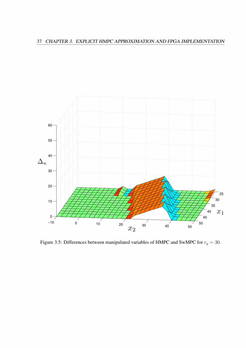
As described in Sec. 3.3, the affine terms in the PWA formulation are con-sidered as constant measured input disturbances in the SwMPC formulation.The target of the controller is to track a reference ry for y = x2, while enforc-ing the constraint x1 ≥ 25 in addition to the constraints in (3.14), (3.16). Thecontrollers (HMPC and SwMPC) share the same tuning parameters: M = 4,Qy = 1, R = 0, ρ = +∞ (corresponding to hard constraints). For a constantreference tracking ry = 30, Figure 3.5 shows that the difference ∆u betweenthe manipulated variables in HMPC and SwMPC is negligible in most of theconsidered points. The controllers characteristics are summarized in Table 3.2.

3.4.2 FPGA implementation

The PWAS approximation of the SwMPC controller has been implemented ona Xilinx Spartan 3 FPGA, using the VHDL language to define the circuit.


The first step towards the FPGA implementation is the PWAS approximationof each explicit linear MPC by applying the method proposed in [10]. Theresult of the approximations are five continuous PWAS functions defined allover the domain, partitioned into simplices using mh = 7 divisions along eachdimensional component.

The second step is to merge the five continuous PWAS functions into onediscontinuous PWAS function fPWAS. Since there are two discontinuities along

x1

−10 0 10 20 30 40 50−10

0

10

20

30

40

50

5

2

3

1

4

x2

mercoledì 13 ottobre 2010

Figure 3.4: PWA state partitions for u = 25C.


25

30

35

40

45

50!10 0 10 20 30 40 50

0

10

20

30

40

50

60

x1

x2

∆u

Thursday, October 14, 2010

Figure 3.5: Differences between manipulated variables of HMPC and SwMPC for ry = 30.


Item HMPC SwMPC(for each controller)

# params 3 (2 states, 1 reference) 3

# variables 36 (12 cont., 24 binary) 6

# inequalities 96 (mixed-integer) 26

# regions N/A 5

# subregions 1385a 10 (maximum),explicit (35 total)

aPossible overlapping regions that are never optimal are not removed

Table 3.2: Controllers dimensions

the first and the second dimensions, the discontinuity partition is composed bynine hyper-rectangular subregionsRi, i = 1, . . . , 9.

Fig. 3.6 shows the input and state signals obtained using the PWAS approx-imated control and the HMPC approach, where a sinusoidal reference ry for x2

is imposed.

Function fPWAS is implemented by resorting to the proposed architecture.To implement the circuit architecture on FPGA we have used a fully genericVHDL description, so that it is possible to change any parameter before pro-gramming the FPGA without editing the VHDL code; these parameters are theinput dimension n, the number of bits used to code the integer part (p) and dec-imal part (q) of the input and the number of bits (b) used to code the coefficientscik. The position of the discontinuities dh,t inside the domain and the value ofthe coefficients cik is set through a Matlab routine that allows the configurationof the whole VHDL code.

The estimated maximum working frequency is 40MHz, that corresponds toa throughput of one sample every 550 ns, with a power consumption of 85mW .


0 5 10 15 20 250

20

40

60

x2,

r

0 5 10 15 20 2520

30

40

50

x1

0 5 10 15 20 2520

30

40

50

u

tt

x1

u

x2, ry

Thursday, October 14, 2010

Figure 3.6: HMPC (blue) vs. PWAS (black).


The approximated discontinuous PWAS control occupies 69% of the hardwareresources of the chosen FPGA.

Chapter 4

Closed-loop stability analysis

The contribution of this Chapter is the definition of a stability analysis frame-work for discrete-time PWA systems subject to both parametric uncertaintiesand additive disturbances which are unknown but bounded and defined in poly-topic sets. The proposed method is based on the use of PWA Lyapunov func-tions synthesized via linear programming, and permits to determine if the stateconverges to the origin (or to a terminal set including the origin). The systemdynamics are defined only in a closed polytopic region X , which is not neces-sarily required to be invariant. By artificially extending the systems dynamicsoutside X , the proposed method can determine an invariant subset of X , inwhich the dynamics of the original PWA system of interest are defined. Theattractiveness of the origin (or that of the terminal set) is determined with re-spect to such a region of attraction. Finally, discontinuities on the boundariesof the partitions are tackled for both the system dynamics and the PWA Lya-punov function, in order to broaden the range of applicability of the proposedapproach and to reduce the conservativeness due to the imposition of continu-ity. The presence of discontinuities, however, requires additional attention ontechnical conditions [26].

41

4.1. PROBLEM FORMULATION 42

Preliminary results of this thesis focusing only on the asymptotic stabilityanalysis of systems without disturbances or with parametric disturbances arereported in [38] and in [42], respectively.

4.1 Problem formulation

Consider the autonomous discrete-time uncertain PWA system

x(k + 1) = Ai(w(k))x(k) + ai(w(k)) + Ei(w(k))d(k) if x(k) ∈ Xi (4.1)

where x(k) ∈ Rn, w(k) ∈ W ⊂ Rq, d(k) ∈ D ⊂ Rp,

Ai(w) , Ai,0 +

q∑

r=1

Ai,rwr (4.2a)

ai(w) , ai,0 +

q∑

r=1

ai,rwr (4.2b)

Ei(w) , Ei,0 +

q∑

r=1

Ei,rwr (4.2c)

W ,w ∈ Rq :

q∑

r=1

wr = 1, wr ≥ 0

(4.2d)

D ,d ∈ Rp : Hd ≤ h

(4.2e)

Ai,r ∈ Rn×n, ai,r ∈ Rn, Ei,r ∈ Rn×p, with r = 0, ..., q, and k ∈ Z+,H ∈ Rp×η, and h ∈ Rη. Denote by d1, . . . , dη ∈ Rp the vertices of D,D = conv(d1, . . . , dη). The sets Xi, i ∈ I , 1, ..., s, are (possibly non-closed) polytopes such that int(Xi) 6= ∅, Xi∩Xj = ∅, ∀i, j ∈ I with i 6= j, andsuch that X , ⋃s

i=1Xi is a closed polytope. The subset of indices I0 is definedas I0 , i ∈ I : 0 ∈ Xi. The interior of each partition Xi is defined as

int(Xi) , x : Hix < hi, i ∈ I (4.3)

43 CHAPTER 4. CLOSED-LOOP STABILITY ANALYSIS

where Hi and hi are a constant matrix and a constant vector, respectively, ofsuitable dimensions, and let Xi the closure of Xi, Xi , x : Hix ≤ hi, i ∈ I.

Denote by

x(k + 1) = Ai,0x(k) + ai,0 if x(k) ∈ Xi (4.4)

the nominal model of (4.1). Note that dynamics (4.1) may not be continuouswith respect to x on the boundaries of the partitions Xi, while it is continuouswith respect to w and d.

Assumption 1. There exists an index i ∈ I such that 0 ∈ vert(Xi), 0 ∈ int(X ).

Note that Assumption 1 can be always satisfied. In fact, if the origin is noton a vertex of any polyhedron Xi, it is always possible to further partition Xto obtain a new set of partitions Xi which fulfills Assumption 1. Note also thatthe state trajectories may not be persistent in time, since X is not necessarily anRPI set, and the dynamics are not defined outside X .

This Chapter addresses the following problem: Given the uncertain PWAsystem (4.1), for which X is not necessarily an RPI set, prove the propertiesof stability and convergence to the origin (asymptotic stability, ultimate bound-edness, and input-to-state stability) with respect to an RPI subset P of X . Incase of ultimate boundedness, find another RPI set F where the state is drivenin finite time.

4.2. REACHABILITY ANALYSIS 44

4.2 Reachability analysis

4.2.1 One-step reachability analysis

Since the set X is not assumed to be RPI with respect to dynamics (4.1), wemust take into account that the trajectories may possibly leave X , and be there-fore defined only on a finite time interval [0, kmax]. Define the one-step reach-able set from X

R(X ) , Ai(w)x+ ai(w) + Ei(w)d : w ∈ W , d ∈ D,x ∈ Xi, i ∈ I

and let

R∪(X ) , R(X ) ∪ X (4.5)

The setR(X ) can be computed as the union of the one-step reachable sets fromall the Xi, defined as

R(Xi) , Ai(w)x+ ai(w) + Ei(w)d, w ∈ W , d ∈ D, x ∈ Xi

Note thatR(Xi) is not a convex set in general. Note that the terms in (4.2a) and(4.2b) can be equivalently expressed as

Ai(w) =

q∑

r=1

(Ai,0 + Ai,r)wr ,q∑

r=1

Ai,rwr

ai(w) =

q∑

r=1

(ai,0 + ai,r)wr ,q∑

r=1

ai,rwr

Ei(w) =

q∑

r=1

(Ei,0 + Ei,r)wr ,q∑

r=1

Ei,rwr


By relying on the results in [12, Chap. 6], we can compute the convex hulls ofthe setsR(Xi) as

conv(R(Xi)

)=

conv(Ai,rvi,h + ai,r + Ei,rdi,µ, r = 1, ..., q, µ = 1, ..., η, h = 1, ...,mi

)

where vi,h represents each of the mi vertices of Xi.Therefore, an over-approximation ofR∪(X ) in (4.5) is

R∪(X ) ,s⋃

i=1

(conv

(R(Xi)

) )∪ X ⊇ R∪(X ) (4.6)

4.2.2 Fake dynamics and extended system

As dynamics (4.1) is not defined outside X , the proposed strategy consists indefining a “fake” dynamics on R∪(X ) \ X . Let XH ⊇ R∪(X ) be the boundingbox of R∪(X ), i.e., the smallest closed hyper-rectangle containing R∪(X ), andconsider the dynamics

x(k + 1) = ρx(k), if x(k) ∈ XE , XH \ X (4.7)

where ρ ∈ [0, 1) is an adjustable parameter of the approach proposed in thisthesis. The region XE can be divided into convex polyhedral regions as in [9,Th. 3]. As a result, new regions Xi, i = s + 1, ..., s, are created. Let I ,1, ..., s. The dynamics of the extended system on XH is

x(k+1) =

Ai(w(k))x(k) + ai(w(k)) + Ei(w(k))d(k) if x(k) ∈ Xi, i ∈ Iρx(k) if x(k) ∈ XE

(4.8)

Lemma 1. The setXH is an RPI set with respect to the extended dynamics (4.8).

4.2. REACHABILITY ANALYSIS 46

Proof. If x ∈ XH , then either x ∈ X or x ∈ XE. If x ∈ X then the successorstate Ai(w)x + ai(w) + Ei(w)d ∈ R∪(X ) ⊆ XH by definition of XH . Ifx ∈ XE, the successor state is ρx ∈ XH , because XH is a convex set includingthe origin.

Defining XH as a bounding box and the dynamics in XE as in (4.7) is asimplistic choice, yet we will prove its effectiveness. Other choices of XH andof the dynamics (4.7) are possible, provided that Lemma 1 holds.

Let x(k) ∈ Xi and x(k + 1) ∈ Xj, (i, j) ∈ I × I. To characterize thetransitions we define the region transition map S

Si,j ,

1 if conv(R(Xi)

)∩ Xj 6= ∅

0 otherwise(4.9)

which states (in a conservative way) whether there exists a state x ∈ Xi and twouncertain vectors w ∈ W , d ∈ D such that Ai(w)x + ai(w) + Ei(w)d ∈ Xj.For any pair (i, j) ∈ I × I, we define

Xi,j ,Xi if S(i,j) = 1

∅ if S(i,j) = 0(4.10)

that we refer to as transition set, representing an overestimate of all the statesthat can possibly end up in Xj in one step under dynamics i. In some particularcases it is possible to give less conservative estimates of such a set of states byusing controllability analysis, as described in the following section.

4.2.3 Case of additive disturbances only

When only additive disturbances affect the system, (4.1) can be written as

x(k + 1) = Ai,0x(k) + ai,0 + Ei,0d(k) (4.11)


For system (4.11), conv(R(Xi)

)= R(Xi) (see e.g. [12, Chap. 6]) and then

R∪(X ) = R∪(X ). As for the definition of the transition sets, it is possible todetermine the subset Xi,j of Xi of states that reach Xj in one step

Xi,j ,x ∈ Xi : ∃d ∈ Di : Ai,0x+ ai,0 + Ei,0d ∈ Xj

(4.12)

We exploit here controllability analysis [12, Chap. 5], and consider the distur-bance vector d as an external input, with respect to which the controllabilityanalysis is carried out. In the augmented state space (x, d) let

Mi(Xi, Xj) =

(x, d) ∈ Rn+p : x ∈ Xi, Ai,0x+ ai,0 + Ei,0d ∈ Xj, d ∈ D

that is computed as

Mi(Xi, Xj) =

(x, d) ∈ Rn+p :

Hi 0

HjAi,0 HjEi,0

0 H

[x

d

]+

0

Hjai,0

0

≤

hi

hj

h

The intersection of Xi with the so-called pre-image set of Xj, representing allthe states that in one step reach Xj under the dynamics and disturbances definedin Xi [12], is calculated as the projection of the setMi(Xi, Xj) onto the statesubspace:

Xi,j =x : ∃d : (x, d) ∈Mi(Xi, Xj)

(4.13)

In case of no additive disturbances we have the nominal case, i.e., we haveto prove asymptotic stability of the PWA system (4.4). For such a form it ispossible to determine exactly which is the partition of Xi which is mapped inXj in one step

Xi,j =

x ∈ Rn :

[Hi

HjAi,0

]x+

[0

Hjai,0

]≤[hi

hj

](4.14)

4.3. PWA LYAPUNOV ANALYSIS FOR THE EXTENDED SYSTEM 48

In both the considered subcases, the transition map (4.9) can be redefined as

Si,j ,

1 if Xi,j 6= ∅0 otherwise

(4.15)

Note that a similar analysis in presence of a disturbance w would lead to a setof bilinear equations (x and w are multiplied to each other), leading to a non-polytopic shape for the regions Xi,j.

4.3 PWA Lyapunov analysis for the extended system

In this section we analyze the asymptotic stability and the ultimate boundednessof the extended system (4.8).

4.3.1 Asymptotic stability

By recalling classical results of stability of nonlinear discrete-time systems (seee.g. [26], [43] and [25, Chap.2]), assume that the origin is an equilibrium pointfor (4.8). Lyapunov stability is guaranteed by the existence of a function V :

XH → R satisfying the conditions

V (x) ≥ α1‖x‖∞ (4.16a)

V (f(x,w, d))− λV (x) ≤ 0 (4.16b)

∀x ∈ Xi and ∀w ∈ W (i ∈ I), where f : Rn × Rq × Rη → Rn is the PWAstate update function defined by (4.8), α1 > 0, λ ∈ (0, 1). Note that (4.16)imply the condition V (0) = 0. Considering (4.16b) in x = 0 and recallingthat 0 is an equilibrium point, f(0, w, d) = 0,∀w ∈ W , ∀d ∈ D, we getV (0)− λV (0) = (1− λ)V (0) ≤ 0, which implies V (0) ≤ 0, and by (4.16a), itfollows that V (0) = 0.


Remark 1. Condition (4.16b) could be replaced by

V (f(x,w, d))− V (x) ≤ −α3‖x‖ (4.17)

where α3 = (1 − λ)α1 > 0. In fact, by (4.16), it follows that V (f(x,w, d)) −V (x) ≤ −(1 − λ)V (x) ≤ −(1 − λ)α1‖x‖. Also, note that the imposition of

an upperbound α2‖x‖ ≥ V (x), α2 > 0, usually found in the literature is not

necessary here, as V is defined over the bounded setXH . As a consequence, it is

always possible to find a-posteriori α2 > 0 such that V (x) ≤ α2‖x‖, ∀x ∈ XH ,

once function V has been determined.

Note that imposing the simpler decreasing condition V (f(x,w, d))−V (x) <

0 for all x ∈ X \ 0 (instead of (4.16b) or (4.17)) does not guarantee the asymp-totic stability of the origin, since the system dynamics are allowed to be discon-tinuous on the boundaries of the partitions Xi. Instead, the fulfillment of (4.16a)and (4.16b) (or (4.17)), even if the resulting Lyapunov function is discontinu-ous, according to [26], is a sufficient condition for the asymptotic stability of(4.8).

The goal is to synthesize a PWA Lyapunov function for system (4.8) satisfy-ing (4.16). Consider the candidate function V : XH → R

V (x) = maxi∈N (x)

Vi(x) (4.18a)

where

N (x) , i ∈ I : x ∈ Xi (4.18b)

and let Vi : Xi → R be defined as

Vi(x) , Fix+ gi (4.18c)


for i ∈ I, where in (4.18c) Fi ∈ R1×n and gi ∈ R are coefficients to bedetermined. Note that simply V (x) = Fix + gi for x ∈ int(Xi). The rationalefor using the max in (4.18a) is that for numerical reasons we want to considerclosed sets Xi and Vi(x), Vj(x) may not coincide on common boundaries Xi∩Xjunless very conservative continuity conditions are imposed.

Since Xi is a convex set and Vi is affine on the corresponding set Xi, it willbe shown that it is enough to impose the Lyapunov conditions (4.16a) only atvert(Xi), and (4.16b) only at vert(Xi,j):

Fivi,h + gi ≥ α1‖vi,h‖ (4.19a)

for all mi vertices vi,h ∈ vert(Xi), i ∈ I, h = 1, . . . ,mi, together with

α1 > 0 (4.19b)

and

Fj(Ai,rvij,h + ai,r) + Ei,rdµ) + gj − λ(Fivij,h + gi) ≤ 0 (4.19c)

for all vij,h ∈ vert(Xi,j), with h = 1, . . . ,mi, for all Ai,r, ai,r, Ei,r withr = 1, ..., q, and all dµ with µ = 1, ..., η. Note that the set generated by theconvex combination of the points Ai,rvij,h + ai,r + Ei,rdµ with respect to thevertices of Xi coincides with conv R (Xi,j). As a consequence, to impose thedecreasing condition (4.19c) one can consider only the vertices of Xi,j gener-ating the vertices of conv R (Xi,j). The resulting constraints (4.19) define alinear feasibility problem in the unknowns Fi, gi, α1, for a fixed decay rate λ,and a feasible solution can be determined by linear programming (LP).

Lemma 2. Let Assumption 1 hold, and let the LP (4.19) associated with the

autonomous uncertain PWA dynamics (4.8) and the candidate Lyapunov func-

tion (4.18) be feasible. Then system (4.8) is UAS(XH).


Proof. As for the positive definiteness of the Lyapunov function, since functionsVi are affine functions defined on convex partitionsXi, the satisfaction of (4.19a)for all vi,h ∈ vert(Xi), with i ∈ I, h = 1, . . . ,mi, for x ∈ Xi leads to

α1‖x‖ = α1

∥∥∥∥∥mi∑

h=1

βi,hvi,h

∥∥∥∥∥ ≤mi∑

h=1

βi,hα1‖vi,h‖

≤mi∑

h=1

βi,h(Fivi,h + gi) = Fi(

mi∑

h=1

βi,hvi,h) + gi

mi∑

h=1

βi,h = Fix+ gi (4.20)

where βi,h ≥ 0,∑mi

h=1 βi,h = 1, are a set of coefficients defining x as a con-vex combination of the vertices of Xi. For this reason, for x ∈ int(Xi), sinceVi(x) = Fix + gi, (4.16a) holds. Moreover, on the boundaries of Xi, accord-ing to (4.18a), one has α1‖x‖ ≤ Fix + gi for all i ∈ N (x), and thereforeα1‖x‖ ≤ maxi∈N (x)Fix + gi = V (x). This implies that (4.16a) holds for allx ∈ XH , since XH =

⋃i∈I Xi.

As for the decay of the Lyapunov function, we have that

V (f(x,w, d)) = Fj

[(q∑

r=1

Ai,rwr

)(mi∑

h=1

βi,hvij,h

)+

q∑

r=1

ai,rwr

+

(q∑

r=1

Ei,rwr

)(η∑

µ=1

cµdµ

)]+ gj (4.21)

with cµ ≥ 0,∑η

µ=1 cµ = 1. Recalling that (4.19c) holds for all the vertices of


Xij, and that∑mi

h=1 βi,h =∑η

µ=1 ch =∑q

r=1wr = 1, from (4.21) we get

V (f(x,w, d)) =Fj

[mi∑

h=1

βi,h

(q∑

r=1

Ai,rwrvij,h

)+

q∑

r=1

ai,rwr

+

(q∑

r=1

Ei,rwr

)(η∑

µ=1

cµdµ

)]+ gj

=Fj

[mi∑

h=1

βi,h

(q∑

r=1

Ai,rwrvij,h

)+

mi∑

h=1

βi,h

(q∑

r=1

ai,rwr

)

+

mi∑

h=1

βi,h

(η∑

µ=1

cµ

(q∑

r=1

Ei,rwrdµ

))]+ gj

=Fj

mi∑

h=1

βi,h

[q∑

r=1

wr

(Ai,rvij,h + ai,r +

η∑

µ=1

cµEi,rdµ

)]+ gj

=Fj

mi∑

h=1

βi,h

[q∑

r=1

wr

(η∑

µ=1

cµAi,rvij,h +

η∑

µ=1

cµai,r +

η∑

µ=1

cµEi,rdµ

)]+ gj

=

mi∑

h=1

βi,h

[q∑

r=1

wr

η∑

µ=1

cµ

(Fj

(Ai,rvij,h + ai,r + Ei,rdµ

))]+ gj

≤mi∑

h=1

βi,h

[q∑

r=1

wr

η∑

µ=1

cµ (λ (Fivij,h + gi)− gj)]

+ gj

=λ

mi∑

h=1

βi,h (Fivij,h + gi)−mi∑

h=1

βi,hgj + gj

=λ

(Fi

mi∑

h=1

βi,hvij,h +

mi∑

h=1

βi,hgi

)= λ (Fix+ gi) = λV (x)

which proves that (4.16b) holds for all x ∈ int (Xi,j). Also, on the boundariesof Xi, the decreasing condition (4.16b) is imposed for all (i, j) ∈ N (x) ×


N (f(x,w, d)), and therefore

maxj∈N (f(x,w,d))

(Fj(f(x,w, d)) + gj

)≤ λ max

i∈N (x)(Fix+ gi)

Since by definition of Xi,j we have that XH =⋃si=1

⋃sj=1Xi,j, (4.16b) holds

for all x ∈ XH . As a result, (4.16) hold for all x ∈ XH , which, following inspirit the proof of Theorem 2.2.1 in [25, Chap. 2] for deterministic systems,guarantees that system (4.8) is UAS(XH) according to Definition 3.

Remark 2. The complexity of the LP (4.19) is the following: there are nv =

1 + s(n+ 1) variables; one inequality is imposed for each vertex of each region

Xi, i = 1, ..., s to fulfill (4.19a); condition (4.19b) introduces one inequality

constraint; to fulfill (4.19c), for each vertex of each region one has to impose

a number of inequalities equal to the number of regions Xj such that Si,j 6= 0,

multiplied by the product q · η; the overall number of constraints is therefore

nc = 1 +s∑

i=1

mi

(1 + q · η · card

(j ∈ I : Si,j = 1

))

Note that asymptotic stability can be proved only if in the regions includ-ing the origin in their closure (0 ∈ Xi) the additive disturbance has no effect,Ei(w) = 0, and the affine terms ai,r = 0, ∀r = 1, ..., q.

4.3.2 Ultimate boundedness

To check ultimate boundedness, we define the following function

V (x) ≥ α1‖x‖∞ (4.22a)

V (0) = 0 (4.22b)


V (f(x,w, d))− λV (x) ≤ δ (4.22c)

where δ ≥ 0, while all the other terms are the same as in (4.16). To study ulti-mate boundedness, infinity norms will be used instead of the generic p-norms.We call a function V : Rn → R satisfying (4.22) a “Lyapunov-like” function.Similarly to (4.19), the constraints

Fivi,h + gi ≥ α1‖vi,h‖∞ (4.23a)

are imposed for all mi vertices vi,h ∈ vert(Xi), i ∈ I, h = 1, . . . ,mi,

Fj(Ai,rvij,h + ai,r + Ei,rdi,µ) + gj − λ(Fivij,h + gi) ≤ δ (4.23b)

for all vij,h ∈ vert(Xi,j), with h = 1, . . . ,mi, for all Ai,r, ai,r, Ei,r with r =

1, ..., q, and all dµ with µ = 1, ..., η. The further constraints

δ ≥ 0 (4.23c)

δ ≤ (1− λ)(L− ε)α1 (4.23d)

gi = 0, i ∈ I0 (4.23e)

α1 > 0 (4.23f)

are also imposed, where L is the minimum distance between the boundary ofthe hyper-rectangle XH and the origin, while 0 < ε 1. Condition (4.23d) isimposed to ensure that the set where the state is ultimately bounded is well de-fined, while (4.23e) ensures the fulfillment of (4.22b). The overall optimizationvector is denoted by ξ, and is composed by δ, α1, and the terms Fi and gi, withi ∈ I.

Lemma 3. Let Assumption 1 hold, and assume that the linear-fractional pro-


gram

minimizeδ

α1(4.24a)

subject to (4.23) (4.24b)

associated with the autonomous uncertain PWA dynamics (4.8) and the candi-

date Lyapunov-like function (4.18) is feasible. Then system (4.8) is UUB(XH ,F),

with

F , x ∈ XH : V (x) ≤ V +F (4.25)

where

V +F = max

x∈convR(Q)V (x) (4.26)

Q =

x ∈ Rn : ‖x‖∞ ≤

δ

(1− λ)α1+ ε

(4.27)

Proof. As for the positive definiteness of the Lyapunov-like function V , theproof is exactly the same as in Lemma 2, in the particular case of infinity norms.To prove (4.22c) is fulfilled for all x ∈ XH , as in Lemma 2, consider the fol-lowing relation

V (f(x,w, d)) =

mi∑

h=1

βi,h

[q∑

r=1

wr

η∑

µ=1

cµ

(Fj

(Ai,rvij,h + ai,r + Ei,rdi,µ

))]+gj

(4.28)By applying the decreasing condition (4.23b) at the vertices of the sets Xi,j, we


obtain

V (f(x,w, d)) ≤mi∑

h=1

βi,h

[q∑

r=1

wr

η∑

µ=1

cµ (δ + λ (Fivij,h + gi)− gj)]

+ gj

=δ + λ

mi∑

h=1

βi,h (Fivij,h + gi)−mi∑

h=1

βi,hgj + gj

=δ + λ

(Fi

mi∑

h=1

βi,hvij,h +

mi∑

h=1

βi,hgi

)

=δ + λ (Fix+ gi)

=δ + λV (x)

which proves that (4.22c) holds for all x ∈ int (Xi,j). Also, on the boundaries ofthe sets Xi, the decreasing condition (4.22c) is imposed for all (i, j) ∈ N (x)×N (f(x,w, d)), and therefore

maxj∈N (f(x,w,d))

(Fj(f(x,w, d)) + gj

)≤ δ + λ max

i∈N (x)(Fix+ gi)

Since by definition of the sets Xi,j we have that XH =⋃si=1

⋃sj=1Xi,j, (4.22c)

holds for all x ∈ XH , and then (4.22) holds for all x ∈ XH .By (4.22a) and (4.22c) it follows that V (f(x,w, d)) − V (x) ≤ −(1 −

λ)V (x)+δ ≤ −(1−λ)α1‖x‖∞+δ = −α3‖x‖∞+δ, where α3 = (1−λ)α1. Bydefinition of Q in (4.27), for all x ∈ XH \ Q we obtain −α3‖x‖∞ + δ < −α3ε,leading to V (f(x,w, d))−V (x) < −α3ε. Then, given λ∗ ∈ R, V (f(x,w, d))−λ∗V (x) < (1−λ∗)V (x)−α3ε ≤ (1−λ∗)V +

H −α3ε, with V +H = maxx∈XH

V (x).In order to get (1 − λ∗)V +

H − α3ε ≤ 0 and λ∗ ∈ (0, 1), it is necessary to im-pose the condition on λ∗ max0, (V +

H − α3ε)/V+H < λ∗ < 1, which is always

feasible, since (V +H − α3ε)/V

+H < 1. In conclusion, we get

V (f(x,w, d))− λ∗V (x) < 0, x ∈ XH \ Q (4.29)


By definition of F , the fulfillment of the constraint (4.23d) implies Q ⊆ XHand, by relying on the invariance of XH (Lemma 1), conv R(Q) ⊆ XH . Thisimplies the max in (4.26) exists and therefore F in (4.25) is well defined.

To prove invariance of F , we distinguish two cases:

• if x ∈ F ∩Q, then f(x,w, d) ∈ conv R(Q) ⊆ F ;

• if x ∈ F \ Q, then (4.29) holds, because F \ Q ⊆ XH \ Q, and thereforeV (f(x,w, d)) ≤ V +

F , meaning that f(x,w, d) ∈ F by definition of F .

Therefore, F is an RPI set for (4.8).Let V −H , infx∈XH\Q V (x) > 0. Then,

∀ x(0) ∈ XH \ Q ∃ k > 0 : V (x(k)) < λk∗V (x(0)) < V −H (4.30)

meaning that x(k) ∈ Q, because XH in an RPI set.Given a ∈ R such that a > δ/α3+ε, let V +

a , maxx(0)∈XH\Q:‖x(0)‖∞≤a V (x(0)).From (4.30), there exists k such that λk∗V (x(0)) ≤ λk∗V

+a < V −H . By letting

k(a) ,

⌊lnV −H − lnV +

a

lnλ∗

⌋(4.31)

we obtain that for all x(0) ∈ XH \ Q with ‖x(0)‖ ≤ a, one has k ≤ k(a). Asa consequence, for any initial condition x(0) ∈ XH \ Q such that ‖x(0)‖ ≤ a,one has x(k + 1) ∈ F , with k ≤ k(a). Being F an RPI set, x(k) ∈ F fork ≥ k(a) + 1.

To finally prove that system (4.1) is UUB(XH ,F), consider a scalar a > 0,and distinguish two cases:

• for all a such that 0 < a ≤ δ/α3 + ε, there exists T (a) = 1 such that, forevery x(0) with ‖x(0)‖∞ ≤ a (i.e. x(0) ∈ Q), x(T ) ∈ F (by definition ofF);


• for all a > δ/α3 +ε, there exists T (a) = k(a)+1 such that, for every x(0)

with ‖x(0)‖∞ ≤ a, x(T ) ∈ F .

In conclusion, for all a > 0, there exists T = T (a) such that, for everyx(0) ∈ XH with ‖x(0)‖∞ ≤ a, x(T ) ∈ F for any admissible sequence ofthe disturbance terms w and d. This implies that system (4.1) is UUB(XH ,F)

according to Definition 4.

As a practical procedure to calculate F , it is possible to partition Q intoa number of subsets Qi, Qi = Xi ∩ Q with i ∈ I. Then, one can obtainconv R(Q) =

⋃si=1 conv R(Qi), with

conv R(Qi) =

convAi,rv

Qi,h + ai,r + Ei,rdi,µ, r = 1, ..., qi, µ = 1, ..., ηi, h = 1, ...,mQi

where vQi,h are the vertices of the sets Qi, and mQi is the number of vertices ofeach Qi. Then, F can be easily computed as the union of the subsets of the Xifor which V (x) ≤ V , i.e.,

F =s⋃

i=1

XFi , XFi , x ∈ Xi : V (x) < V (4.32)

Remark 3. The aim of (4.24a) is to minimize the volume of the hypercubeQ for

the given choice of the partitions, in order to obtain a set F that is as small as

possible. Note that (4.24) is a quasi-convex optimization problem. Even though

quasi-convex optimization problems are solved in general by bisection (solving

a convex optimization problem at each step), linear-fractional programs like

(4.24) can be transformed into an equivalent LP using the following procedure

(see [16, Chap. 4] for a formal proof).


Assume that δ and α1 are, respectively, the first and second components of

the optimization vector ξ in (4.24). Let Meqξ = 0 denote the whole set of

equality constraints (4.23e) and Minξ ≤ min the whole set of inequality con-

straints (4.23a)-(4.23d), where Meq, Min, and min can be easily constructed

from (4.23). Moreover, rewrite (4.23f) as e′ξ > 0, with e = [0 1 0 . . . 0]′. Prob-

lem (4.24) is therefore equivalent to the following linear-fractional program

minimizec′ξ

e′ξ

subject to Minξ ≤ min

Meqξ = 0

e′ξ > 0 (4.33)

where c = [1 0 . . . 0]′. If the feasible set of (4.33) is not empty, an equivalent

LP of (4.33) is

minimize c′y

subject to Miny −minz ≤ 0

Meqy = 0

e′y = 1

z ≥ 0 (4.34)

where y has the same dimension as ξ and z ∈ R. The optimal vector of (4.24)is ξ = 1

zy.

Remark 4. The number of variables and constraints in (4.34) is comparable

with that of (4.19). In particular, two more variables are added, leading to

nv = 3 + s(n + 1). To define Meqy = 0, one equality constraint is imposed

for each region Xi such that 0 ∈ Xi. One inequality is imposed for each vertex


of Xi, i = 1, ..., s to fulfill (4.23a). To fulfill (4.23b), for each vertex of each

region it is necessary to impose a number of inequalities equal to the number of

regions Xj such that Si,j 6= 0, multiplied by q · η. Condition (4.23c) and (4.23d)introduce two more inequality constraints, while two other constraints are in-

troduced in the auxiliary problem (4.34). The overall number of constraints is

overall number of scalar constraints is

nc = 4 + card(I0) +s∑

i=1

mi

(1 + q · η · card

(j ∈ I : Si,j = 1

))

4.3.3 Feasibility issues

In case (4.19) or (4.23) is infeasible, besides increasing the value of λ, a possi-bility is to increase the number of partitions Xi of XH , therefore providing moreflexibility in synthesizing the PWA Lyapunov (or Lyapunov-like) function.

PWQ Lyapunov function synthesis approaches [20] assume that V is quadraticon each cell Xi. On the other hand, assuming that V is affine on each Xi wouldnot provide enough degrees of freedom. Therefore, for each polyhedron Xi, itsDelaunay triangulation [44] XD

i,1, . . . ,XDi,ni, i ∈ s is computed. The PWA Lya-

punov synthesis procedure is performed by replacing the sets Xi with the ele-ments of the simplicial partition XD

1,1, . . . ,XD1,n1

,XD2,1, . . . ,XD

2,n2, . . . ,XD

s,1, . . . ,

XDs,ns, and consequently by setting I = 1, . . . ,∑s

i=1 ni, and I the subset ofI of indices for which Xi ⊆ X .

An alternative way, which is only applicable in the absence of multiplicativedisturbances (Section 4.2.3), is to consider the sets Xi,j as the new sets Xi andrestart the procedure. Alternatively, in case Xi are simplices, one can split each


of them into n+ 1 new simplices by considering the midpoint v = 1n+1

∑ni=0 vi

as a new vertex. Note that by iterating such procedures, the complexity of theLP (4.19) or (4.23) grows quite fast.

4.4 Invariance analysis

So far the properties of the extended system (4.8) were analyzed. As this in-cludes the fake dynamics (4.7), we want to derive now conditions on the orig-inal system (4.1). Consider again system (4.8) in XH , assume that a feasiblesolution to (4.19) or to (4.23) exists, define

V −E , infx∈XE

V (x) (4.35)

and consider the subset P of X

P , x ∈ X : V (x) < V −E (4.36)

Note that the set P may not be convex, not even connected.The results for the extended system (4.8) proved in Lemmas 2 and 3 and the

definition of P in (4.36) are exploited next to state the main results of the thesis.

Theorem 1. Consider system (4.1), whose dynamics are defined on X , and

assume that the extended dynamics (4.7) are defined in XE. If a Lyapunov

function for system (4.8) is found by solving the LP (4.19), P ⊆ X defined

in (4.36) is an RPI set for (4.1). Moreover, (4.1) is UAS(P).

Proof. The proof consists in showing that the PWA Lyapunov function

VUAS(x) , V (x), ∀x ∈ P (4.37)

where V (x) is found as in Lemma 2 for the extended system (4.8) in XH , is aLyapunov function for (4.1) over the set P . First of all, considering that P is

4.4. INVARIANCE ANALYSIS 62

an RPI set for (4.8) in XH , one can note that the state update f(x,w, d) ∈ Pfor x ∈ P is always given by (4.1). Then, P is an RPI set for (4.1), becausethe dynamics (4.7) is never executed. Considering that P ⊆ XH , if (4.16) aresatisfied for all x ∈ XH (and then for all x ∈ P), we conclude that VUAS(x) is aLyapunov function for system (4.1) in P , and that system (4.1) is UAS(P).

Theorem 2. Consider system (4.1) on X , and assume that dynamics (4.7) are

defined in XE. If a Lyapunov-like function for system (4.8) is found by solving

the LP (4.34), and F ⊆ P (i.e. V −E ≥ V +F ), the sets P ⊆ X and F ⊆ P are

RPI sets with respect to dynamics (4.1). Moreover, system (4.1) is UUB(P ,F).

Proof. The proof consists in showing that the PWA Lyapunov-like function

VUUB(x) , V (x), ∀x ∈ P (4.38)

where V (x) is found as in Lemma 3 for (4.8) in XH , is a Lyapunov-like func-tion for (4.1) over the set P . Being P an RPI set for (4.8) in XH , the stateupdate f(x,w, d) ∈ P for x ∈ P is always calculated using dynamics (4.1),and then P is an RPI set also with respect to the dynamics (4.1), because dy-namics (4.7) is never executed. Considering that P ⊆ XH , if (4.22) hold for allx ∈ XH (and then for all x ∈ P), the invariance of F is guaranteed by Lemma3. Also, since we already proved that P is invariant, it follows that system (4.1)is UUB(P ,F).

The overall procedure proposed in this thesis for uniform asymptotic stabilityis summarized in Algorithm 1, while Algorithm 2 summarizes the procedure foruniform ultimate boundedness.

As a practical procedure to represent the set P , one can define the polyhedra

X Pi , x ∈ Xi : V (x) < V −E , i = 1, ..., I, (4.39)


Algorithm 1: Uniform asymptotic stability analysisInput: PWA system (4.1)Output: Region of attraction P and certificate of UAS(P) for system (4.1)repeat

if a given maximum number of iterations is exceeded thenP undefined;STOP

Obtain new regions Xi by splitting the existing regions;Compute R∪(X ) in (4.6) and XH ;Define the fake dynamics (4.7);Find S in (4.9) or (4.15), and the Xi,j in (4.10), (4.13) or (4.14);Solve the LP feasibility problem (4.19);

until the LP has a solution;Find the region of attraction P ⊆ X ;System (4.1) is UAS(P)

and define the invariant set P as

P =I⋃

i=1

X Pi (4.40)

4.5 Input-to-State Stability

In addition to the properties analyzed in the previous sections, the ISS proper-ties of PWA systems of the form (4.11) can be analyzed. System (4.4) can beextended to the set XH , obtaining

x(k + 1) =

Ai,0x(k) + ai,0 if x(k) ∈ Xi, i ∈ Iρx(k) if x(k) ∈ XE

(4.41)

which is a particular case of (4.8). According to [26], it is possible to deter-mine if a system in form (4.11) is ISS relying on the asymptotic stability of the

4.5. INPUT-TO-STATE STABILITY 64

Algorithm 2: Uniform ultimate boundedness analysisInput: PWA system (4.1)Output: Region of attraction P , set F , and certificate of UUB(P ,F) for system (4.1)repeat

if a given maximum number of iterations is exceeded thenP and F undefined;STOP

repeatif a given maximum number of iterations is exceeded thenP and F undefined;STOP

Obtain new regions Xi splitting the existing regions;Compute R∪(X ) in (4.6) and XH ;Define the fake dynamics (4.7);Find S in (4.9) or (4.15), and the Xi,j in (4.10), (4.13) or (4.14);Solve the LP (4.34);

until the LP has a solution;find F ;

until F ⊆ P;System (4.1) is UUB(P ,F)


nominal system (4.4). To this purpose, we define the set of all possible additivedisturbance realization for (4.11), as

D′ , d′ ∈ Rn : d′ = Eid, d ∈ D, i ∈ I (4.42)

The following result holds:

Theorem 3. Let D′ ⊆ B∞χ , for a given χ > 0. Let the set P∗ ⊆ X with

0 ∈ int(P∗) be defined such that, for system (4.11), R(P∗) ⊕ B∞χ ⊆ P∗.Suppose that the nominal extended system (4.41) is proved to be UAS(XH)

solving the LP (4.19), and (4.4) is UAS(P∗). Then, system (4.11) is ISS(P∗).

Proof. The result immediately follows by taking into account that the invokedassumptions lead to the fulfillment of the assumptions of Proposition IV.2 in[26].

The main problem to check ISS is to define the set P∗. A simple choiceconsist of taking P∗ = P , with P defined in (4.36) for the nominal system(4.4). For this simple choice, Algorithm 3 gives a procedure to check the ISSproperty.

Algorithm 3: Input-to-state stability analysisInput: PWA systems (4.11) and (4.4)Output: Region of attraction P and certificate of ISS(P) for system (4.11)Run Algorithm 1 with system (4.4) as input and get P;Compute B∞χ as the smallest B∞χ such that B∞χ ⊇ D′;ifR(P)⊕B∞χ ⊆ P for the dynamics (4.11) then

system (4.11) is ISS(P)

4.6. SIMULATION EXAMPLES 66

4.6 Simulation examples

An interesting application of PWA stability analysis is to prove closed-loop sta-bility properties of control systems composed by a linear (or PWA) system anda linear (or PWA) controller. In particular, the proposed stability and invarianceanalysis procedure is tested on the closed-loop system composed by a discrete-time PWA system and a switched explicit linear MPC controller (see, e.g., [33]).

The second-order open-loop PWA system is defined by

x(k + 1) = Aj(w(k))x(k) +Bju(k) + Ejd(k) if x(k) ∈ Ωj, (4.43)

where j = 1, 2, x(k) ∈ Ωi ⊂ R2, w(k) ∈ W ⊂ R2, d(k) ∈ D ⊂ R2 with

Aj(w) , Aj,0 + Aj,1wj,1 + Aj,2wj,2

W ,w ∈ R2 : w1 + w2 = 1, w1, w2 ≥ 0

D ,d ∈ R2 : d1 + d2 = 0, ‖d‖∞ ≤ 0.1

More specifically, we have

A1,0 = KA ·[

0.7 0.7

0 0.7

], A2,0 =

[0.6 0.6

0 0.6

], KA ∈ R+

A1,1 =

[0 0.1

0 0

], A2,1 =

[0 −0.2

0 0

]

A1,2 =

[0 0

0 −0.1

], A2,2 =

[0 0

0 0.2

]

B1 =

[1.1

0

], B2

[0.9

0

]

E1 = E2 =KE ·[

1 0

0 1

], KE ∈ R+


where KA and KE are scalar parameters to be assigned.

The regions Ωi are defined by Ω1 = x ∈ R2 : H1x ≤ h1, Ω2 = x ∈ R2 :

H2x ≤ h2 \ Ω1, with

H1 =

0 0.1

0 −0.1

−0.1 0

1 0

, H2 =

0 0.1

0 −0.1

−1 0

0.1 0

h1 =

1

1

1

−1

, h2 =

1

1

1

1

and the whole set where the system dynamics are defined is X = Ω1 ∪ Ω2.The switched explicit linear MPC controller is defined by computing an explicitMPC control law [9] uj(x) for each nominal linear system

x(k + 1) = Aj,0x(k) +Bju(k)

and by setting

u(k) = uj(k) if x(k) ∈ Ωj (4.44)

with a prediction horizon N = 5, a control horizon Nu = 2, weight matrices

Q =

[1 0

0 10

], R = 0.1

on the state and the control, respectively, and terminal weight matrices Pj ∈ R2

found as the solution of the Lyapunov equation A′j,0PAj,0 − P = −Q on eachpartition Ωj. The control constraints are u ∈ [−4, 4], and the state constraints


x ∈ X , are also imposed as soft constraints in solving the multiparametricprograms to obtain the control law (4.44).1

The overall closed-loop system, which does not have any a priori stabilityproperties, can be written in form (4.1). In this case, the partitions Xi are thoseautomatically generated by the multiparametric programming solver that deter-mines the PWA functions uj : Ωj → R, j = 1, 2. Three different stabilityanalysis problems are considered below.

4.6.1 Uniform asymptotic stability

Assume that the additive disturbance is not present in (4.43) (KE = 0). As-sume also KA = 1. The set X is not invariant for the considered overallPWA closed-loop system. For instance, starting at an initial condition x(0) =[−10 −9.5

]′∈ X , the explicit MPC control variable is u(0) = 4. With a dis-

turbance vector w(0) =[0.9 0.1

]′, it yields x(1) =

[−10.11 −6.56

]/∈ X . In

this case, we can verify if the closed-loop system is UAS in a setP ⊆ X . There-fore, we find R∪(X ) in (4.6) and its bounding box XH , with the extended dy-namics (4.8) defined with ρ = 0.99. The regions obtained using the switched ex-plicit MPC, together with the extension given by XH \X , are shown in Fig. 4.1.

According to Algorithm 1, we found the transition map S in (4.9), the tran-sition sets Xi,j in (4.10), and solved the LP (4.19) with λ = 0.99, proving thatthe closed-loop system is UAS(P). The LP is composed of 691 constraints and76 variables, and solved using CPLEX in 7.3 ms on a 2.4 GHz processor. The

1Note that the linear MPC control laws are defined for all x ∈ R2. The multiparametric program is solved onlyfor x(k) ∈ X , and predictions x(k+ t), t = 1, ..., N , may exit X . In order to allow this, the constraints x ∈ X aresoftened.


Figure 4.1: The invariant set XH for case A is constituted by the union of the regions of theexplicit MPC and the box XH \ X (the grey rectangle on the left)


x2x1

V (x)

Wednesday, March 30, 2011

Figure 4.2: The PWA Lyapunov function for the extended system in case A


x2

x1

Wednesday, March 30, 2011

Figure 4.3: The invariant set P obtained in case A


corresponding Lyapunov function is shown in Figure 4.2 and the RPI set P isshown in Figure 4.3.

4.6.2 Uniform ultimate boundedness

Assume now that both parametric and additive disturbances are present, withKA = 1 and KE = 10−2. Even though the additive disturbance is a relativelysmall one, we already know that the system is not uniformly asymptoticallystable in any subset of X . However, we can verify if the closed-loop system isUUB from a set P ⊆ X to a set F ⊆ P . Therefore, we find R∪(X ) in (4.6) andits bounding box XH , with the extended dynamics (4.8) defined with ρ = 0.99,as in case A. According to Algorithm 2, the transition map S in (4.9) and thetransition sets Xi,j in (4.10) are found. Then, the LP (4.34) is solved with λ =

0.99, proving that the closed-loop system is UUB(P ,F). The LP is composedof 1308 constraints and 78 variables, and solved using CPLEX in 8.6 ms ona 2.4 GHz processor. The corresponding Lyapunov-like function is shown inFigure 4.4, while Figure 4.5 shows the invariant set P and the terminal set F .

4.6.3 Input-to-state stability

Finally, assume that the parametric disturbance w is not present in (4.43), i.e.Ai,j = 0, i, j = 1, 2. Moreover, KA = 0.9 and KE = 20. In this case, it is pos-sible to check the ISS of the system with respect to the additive disturbance. Theset D′ in (4.42) is easily found as D′ ,

d′ ∈ R2 : d1 + d2 = 0, ‖d‖∞ ≤ 2

.

According to Algorithm 3, we found the transition map S in (4.15) and thetransition sets Xi,j in (4.14) for the nominal closed-loop system. The feasibilityproblem (4.19) with λ = 0.99 is composed of 435 constraints and 73 variables,


x2x1

V (x)

Tuesday, March 29, 2011

Figure 4.4: The PWA Lyapunov-like function for the extended system in case B


x1

x2


Figure 4.5: The invariant set P and the terminal set F (shaded) in case B


and solved using CPLEX in 3.0 ms on a 2.4 GHz processor. Since the prob-lem admits a solution, the system is proved to be UAS(X ), i.e. X ≡ P isalready an RPI set. The set B∞χ is equal to B∞2 , and therefore we can computeR(P) ⊕B∞2 . The result is shown in Fig. 4.6, where it is possible to see thatR(P)⊕B∞2 ⊂ P . We can conclude that the closed-loop system is ISS(X ).


x2

x1


Figure 4.6: The sets P ≡ X andR(P)⊕B∞2 (in black) in case C

Chapter 5

Conclusion

For hybrid MPC controllers approximated as switched linear MPC controllerswe have proposed an architecture to evaluate discontinuous PWAS functions byextending the architecture proposed in [40]. The implementation requires theintroduction of comparators and 1-bit adders which are very simple and fastdevices and so is remarkably efficient. This fact is a direct consequence of thechosen class of discontinuous functions. Thus, our circuit represents a goodtrade-off between model complexity and circuit performances in terms of areaoccupation and power consumption. A further generalization of the proposedarchitecture can be obtained by using a binary-tree search [23,31] instead of thebank of comparators. In this case, we could implement discontinuous functionsthat are continuous over non hyper-rectangular regions, at the cost of a morecomplex circuit.

Also, this work has addressed the problem of determining the properties ofuniform asymptotic stability, uniform ultimate boundedness, and input-to-statestability of (possibly discontinuous) uncertain discrete-time PWA systems, sub-ject to both additive and parametric disturbances. Since the dynamics are de-fined in the set X that is a-priori not invariant, a partially fictitious dynamics is

77

78

exploited to define a (possibly discontinuous) PWA Lyapunov functions, lead-ing to the formulation of an LP. As an outcome of the optimization problem, theRPI set P ⊆ X is obtained, together with the terminal set F , in case uniformultimate boundedness is analyzed. The reported simulation examples, althoughreferring to a second-order system for the sake of simplicity, confirm the lowcomputational burden required to solve the LPs associated with the proposedmethod, therefore making the proposed method amenable for analysis of morecomplex systems arising in real-life control applications.

Open problems and suggestions

In this thesis, the stability analysis problem was formulated and solved usingPWA Lyapunov function, as well as the synthesis of PWA controllers throughFPGA. Since the flexibility of such functions, it would be subject of further in-terest to analyze the synthesis problem. Many are the applications that wouldreceive benefit in terms of simplicity of controller synthesis step, after the plantdesign. As an example, when dealing with vehicular systems, a large mixtureof state machines and dynamical models are involved in the controller designsteps. The design can be simplified using the hybrid MPC approach, and, wherethe resulting controller is too complex, using the switched MPC approach. Also,since the large-scale models, a large-scale stability problem arises in such cases.It would be an important step forward to develop an algorithm able to synthe-size a switched MPC such that the closed-loop is stable. In this way, one caninherit the controller’s performance together with the simplicity of tuning of thesingle MPC, digging and searching for the optimal tuning in a stable class ofcontrollers.

79 CHAPTER 5. CONCLUSION

Bibliography

[1] A. Alessio and A. Bemporad. A survey on explicit model predictive con-trol. In L. Magni, F. Allgower, and D. M. Raimondo, editors, Nonlinear

Model Predictive Control: Towards New Challenging Applications, vol-ume 384, pages 345–369. Berlin Heidelberg, 2009.

[2] A. Bemporad. Efficient conversion of mixed logical dynamical systemsinto an equivalent piecewise affine form. IEEE Transactions on Automatic

Control, 49(5):832–838, 2004.

[3] A. Bemporad. Hybrid Toolbox - User’s Guide, 2004.http://www.ing.unitn.it/ bemporad/hybrid/toolbox.

[4] A Bemporad. Model predictive control design: New trends and tools. 45th

IEEE Conference on Decision and Control, pages 6678–6683, 2006.

[5] A Bemporad, F Borrelli, and M Morari. Model predictive control basedon linear programming - the explicit solution. IEEE Transactions on Au-

tomatic Control, pages 1–12, Jul 2001.

[6] A. Bemporad, W. Heemels, and B. De Schutter. On hybrid systems andclosed-loop MPC systems. IEEE Transactions on Automatic Control,47(5):863–869, 2002.

81

BIBLIOGRAPHY 82

[7] A. Bemporad and M. Morari. Control of systems integrating logic, dy-namics, and constraints. Automatica, 35(3):407–428, 1999.

[8] A Bemporad and M Morari. Robust model predictive control: A survey.Lecture notes in control and information sciences, pages 207–226, 1999.

[9] A. Bemporad, M. Morari, V. Dua, and E. N. Pistikopoulos. The explicitlinear quadratic regulator for constrained systems. Automatica, 38(1):3–20, 2002.

[10] A. Bemporad, A. Oliveri, T. Poggi, and M. Storace. Ultra-fast stabilizingmodel predictive control via canonical piecewise affine approximations.IEEE Trans. Autom. Control., 2011. In press.

[11] P. Biswas, P. Grieder, J. Lofberg, and M. Morari. A survey on stabilityanalysis of discrete-time piecewise affine. In Proceedings of 16th IFAC

World Congress, Praha, Czech Republic, June 2005.

[12] F. Blanchini and S. Miani. Set-theoretic methods in control. Springer,2008.

[13] L. G. Bleris, P. D. Vouzis, M. G. Arnold, and M. V. Kothare. A co-processor FPGA platform for the implementation of real-time model pre-dictive control. In Amer. Control Conf., Minneapolis, MN, June 2006.

[14] F. Borrelli, M. Baotic, A. Bemporad, and M. Morari. Dynamic program-ming for constrained optimal control of discrete-time linear hybrid sys-tems. Automatica, 41(10):1709–1721, 2005.

[15] S. Boyd, L. El Ghaoui, E. Feron, and V. Balakrishnan. Linear matrix

inequalities in system and control theory. SIAM, 1994.

83 BIBLIOGRAPHY

[16] S. P. Boyd and L. Vandenberghe. Convex Optimization. Cambridge Uni-versity Press, 2004.

[17] F. J. Christophersen, M. Baotic, and M. Morari. Stability analysis of hybridsystems with a linear performance index. In IEEE Conference on Decision

and Control, Atlantis, Paradise Island, Bahamas, December 2004.

[18] S. Di Cairano, H. E. Tseng, D. Bernardini, and A. Bemporad. Steeringvehicle control by switched model predictive control. In 6th IFAC Symp.

Adv. Automotive Control, Munich, Germany, July 2009.

[19] P. Echevarria, M. V. Martınez, J. Echanobe, I. del Campo, and J. M. Tarela.Digital hardware implementation of high dimensional fuzzy systems. InApplications of Fuzzy Sets Theory, Lecture Notes in Computer Science,pages 245–252. Springer, Berlin, 2007.

[20] G. Ferrari-Trecate, F. A. Cuzzola, D. Mignone, and M. Morari. Anal-ysis of discrete-time piecewise affine and hybrid systems. Automatica,38(12):2139–2146, December 2002.

[21] HJ Ferreau, HG Bock, and M Diehl. An online active set strategy to over-come the limitations of explicit mpc. International Journal of Robust and

Nonlinear Control, 18(8):816–830, 2008.

[22] P. Grieder, M. Kvasnica, M. Baotic, and M. Morari. Stabilizing low com-plexity feedback control of constrained piecewise affine systems. Auto-

matica, 41(10):1683–1694, 2005.

[23] T. A. Johansen, W. Jackson, R. Schreiber, and P. Tøndel. Hardware synthe-sis of explicit model predictive controllers. IEEE Transaction on Control

System Technology, 15(1):191–197, Jan. 2007.

BIBLIOGRAPHY 84

[24] E. C. Kerrigan and D. Q. Mayne. Optimal control of constrained, piece-wise affine systems with bounded disturbances. In Conference on Decision

and Control, Las Vegas, NV, December 2002.

[25] M. Lazar. Model predictive control of hybrid systems: stability and ro-

bustness. PhD thesis, Eindhoven University of Technology, Eindhoven,The Netherlands, 2006.

[26] M. Lazar, W. P. M. H. Heemels, and A. R. Teel. Lyapunov functions, sta-bility and input-to-state stability subtleties for discrete-time discontinuoussystems. IEEE Transactions on Automatic Control, 54(10):2421–2425,2009.

[27] H. Lin and P.J. Antsaklis. Synthesis of uniformly ultimate boundednessswitching laws for discrete-time uncertain switched linear systems. InProc. Conference on Decision and Control, Maui, HI, December 2003.

[28] K. Ling, B. Wu, and J. Maciejowski. Embedded model predictive control(MPC) using a FPGA. In Proc. 17th IFAC World Congress, pages 15250–15255, Seoul, Korea, July 2008.

[29] K. V. Ling, S. P. Yue, and J. Maciejowski. A FPGA implementation ofmodel predictive control. In Amer. Control Conf., Minneapolis, MN, June2006.

[30] D Mayne and J Rawlings. Constrained model predictive control: stabilityand optimality (vol 36, pg 789, 2000). Automatica, 36:789–814, Jan 2001.

[31] A. Oliveri, A. Oliveri, T. Poggi, and M. Storace. Circuit implementation ofpiecewise-affine functions based on a binary search tree. In Proc. Europ.

85 BIBLIOGRAPHY

Conf. Circ. Th. Design (ECCTD’09), pages 145–148, Antalya, Turkey,August 23-27 2009.

[32] M. Parodi, M. Storace, and P. Julian. Synthesis of multiport resistors withpiecewise-linear characteristics: a mixed-signal architecture. Int. J. Circ.

Th. Appl., 33(4):307–319, 2005.

[33] T. Poggi, S. Trimboli, A. Bemporad, and M. Storace. Explicit hybridmodel predictive control: discontinuous piecewise-linear approximationand FPGA implementation. In IFAC World Congress, Milan, Italy, August2011.

[34] S. Prajna and A. Papachristodoulou. Analysis of switched and hybridsystems-beyond piecewise quadratic methods. In Proc. American Control

Conference, Denver, CO, June 2003.

[35] S. V. Rakovic, E. C. Kerrigan, K. I. Kouramas, and D. Q. Mayne. Invari-ant approximations of the minimal robust positively invariant set. IEEE

Transactions on Automatic Control, 50(3):406–410, 2005.

[36] A. Richards, W. Stewart, and A. Wilkinson. Auto-coding implementationof model predictive control with application to flight control. In Proc.

Europ. Control Conf. 2009, Budapest, Hungary, August 2009.

[37] R. Rovatti, C. Fantuzzi, and S. Simani. High-speed DSP-based implemen-tation of piecewise-affine and piecewise-quadratic fuzzy systems. Signal

Processing, 80:951–963, 2000.

[38] M. Rubagotti, S. Trimboli, D. Bernardini, and A. Bemporad. Stability andinvariance analysis of approximate explicit MPC based on PWA Lyapunovfunctions. In 18th IFAC World Congress, Milan, Italy, August 2011.

BIBLIOGRAPHY 86

[39] E. D. Sontag. Nonlinear regulation: The piecewise linear approach. IEEE

Transactions on Automatic Control, 26(2):346–358, 1981.

[40] M. Storace and T. Poggi. Digital architectures realizing piecewise-linearmulti-variate functions: two FPGA implementations. Int. J. Circ. Th.

Appl., 37, 2010. in press, doi: 10.1002/cta.610.

[41] P. Tøndel, T. A. Johansen, and A. Bemporad. Evaluation of piecewiseaffine control via binary search tree. Automatica, 39(5):945–950, 2003.

[42] S. Trimboli, M. Rubagotti, and A. Bemporad. Stability and invarianceanalysis of uncertain PWA systems based on linear programming. In Proc.

Conference on Decision and Control, 2011.

[43] M Vidyasagar. Nonlinear systems analysis. Prentice-Hall, 1993.

[44] L. Yepremyan and J. E. Falk. Delaunay partitions in Rn applied to non-convex programs and vertex/facet enumeration problems. Computers and

Operations Research, 32(4):793–812, 2005.

[45] G. Zhai, H. Lin, and P. J. Antsaklis. Quadratic stabilizability of switchedlinear systems with polytopic uncertainties. International Journal of Con-

trol, 76(7):747–753, 2003.

Documents

DISI - University of Trento Approximate Explicit MPC and …eprints-phd.biblio.unitn.it/823/1/PhD-Thesis-Trimboli.pdf · · 2012-12-02PhD Dissertation International ... cial PWA