Embed Size (px)
Citation preview
The Pennsylvania State University
The Graduate School
Department of Electrical Engineering
DISPERSION AND DISTRIBUTION OF
OPTICAL INDEX OF REFRACTION IN
FERROELECTRIC RELAXOR CRYSTAL
A Thesis in
Electrical Engineering
by
Chunlai Li
© 2006 Chunlai Li
Submitted in Partial Fulfillment of the Requirements
for the degree of Doctor of Philosophy
May 2006

The thesis of Chunlai Li has been reviewed and approved* by the following
Date of Signature
Ruyan Guo Professor of Electrical Engineering and Materials Research Thesis Co-Advisor Co-Chair of Committee
Amar S. Bhalla Professor of Materials and Electrical Engineering Thesis Co-advisor Co-Chair of Committee
Leslie Eric Cross Evan Pugh Professor Emeritus of Electrical Engineering
William B. White Professor Emeritus of Geochemistry
Shizhuo Yin Associate Professor of Electrical Engineering
W. Kenneth Jenkins Professor of Electrical Engineering Head of the Department of Electrical Engineering
*Signatures are on file in the graduate school
iii
Abstract
This thesis deals with the optical properties of relaxor ferroelectrics with
nano/micro polar regions, including their optical frequency dispersion near phase
transition, thermo-optical properties, and transmission spectrum analysis. The essential
objectives of this thesis work are to deepen the understanding on diffuse phase transition
of relaxor ferroelectrics and to obtain practical data for potential optical application from
technically important ferroelectrics crystals PBN and PZN-PT.
Temperature dependent birefringence and optical refractive indices of PBN (Pb1-
xBaxNb2O6) crystal (1-x=0.57) were measured in several optical wavelengths (λ= 694nm,
633nm, 535nm, and 450nm) to understand the optical frequency dependency of
ferroelectric phase transitions in relaxor ferroelectric crystals of tungsten bronze
structure. Local polarization is verified to be dynamically activated by thermal process
and probed effectively by suitable wavelength of light. An optical isotropic point, as a
function of temperature and light frequency, is reported at which the crystal’s standing
birefringence is fully compensated by polarization. A modified single oscillator model is
used to calculate the index of refraction in the ferroelectric phase. The deviation
temperature from the single oscillator model is reported to be significantly marking the
crossover from macroscopic to microscopic polarization. A new parameter, optical Curie
temperature region, defined by the temperature difference between the well known Burns
temperature and the deviation temperature (from the single oscillator model for index of
refraction) is explored for its significance in depolarization behavior of the micro- to
nano-polar regions of the ferroelectric relaxor.
iv
Temperature dependent optical indices of refraction of PZN-0.12PT (1-
x)PbZn1/3Nb2/3O3-xPbTiO3, x=0.12, were also studied with emphasis on poling effect.
The refractive index n3 decreases as a result of [001] poling. Temperature dependent
effective energy of dispersion oscillator 0E and dispersion energy dE were calculated
using single oscillator model and found that 0E and dE increased by 32% and 60% after
[001] poling, respectively. Birefringence of poled PZN-0.12PT also was measured with
several frequencies and varying temperature. The polarization derived from refractive
index and birefringence were consistent with each other. The remnant polarization was
increased by approximately 30% as a result of [001] poling. Transmission spectrum of
PZN-0.12PT was measured from near UV to IR for both poled sample and unpoled
sample. Transmission was improved significantly after poling. By analyzing the
transmission spectrum in the visible range, optical band gap and lattice phonon were
determined. The existence of hydrogen in PZN-0.12PT single crystal grown by flux
method was postulated based on evidence obtained by FTIR.
For accurate and fast birefringence measurement, which is of fundamental
importance to device design, quality control, and various sensing functions, a two-
dimensional birefringence profiling and analysis system was designed and implemented
successfully. Jones matrices of two and three 90° domains are derived and conclude that
odd number of stacked 90° domains can be treated as a single 90° domain while even
number of stacked 90° domains can be treated as two 90° domains. By rotating analyzer
method a test experiment using voltage controllable liquid crystal as sample is
demonstrated.
v
Table of Contents
List of Tables.………………………………………………………………………...….ix
List of Figures..……………………………………………………………………..…….x
Acknowledgments………………………………………………………………………xiv
Chapter 1. Introduction
1.1 Introduction of ferroelectrics……………………………………………...1
1.1.1 Ferroelectrics………………………………………………………..1
1.1.2 General properties of ferroelectrics…………………………………2
1.1.2.1 Crystal symmetry……………………………………………2
1.1.2.2 Phase transition……………………………………………...4
1.1.2.3 Domain and hysteresis………………………………………5
1.2 Relaxor ferroelectrics……………………………………………………..8
1.2.1 Structure of relaxor ferroelectrics……………………………...…..10
1.2.2.1 Perovskite structure………………………….………...…..10
1.2.2.2 Tungsten bronze structure…………………………………11
1.2.2 Dielectric and related properties…………………………………..15
1.2.3 Optical properties……………………………………………….…17
1.3 Domain in ferroelectrics…………………………………………………19
1.3.1 Ferroelectric domain……………………….………………………19
1.3.2 Domain investigation……………….…….………………………..20
1.3.3 Size effect…………………………………………………………23
vi
1.4 Review of various models of relaxor ferroelectrics…………………….24
1.4.1 First principles calculation………………………………………...25
1.4.2 Compositional fluctuation model theory……………….……….…27
1.4.3 Superparaelectricity model theory………………………………....31
1.4.4 Dipolar glass model ……………………………………………….34
1.4.5 Random fields theory………………………………………………36
1.5 Optical properties………………………………………………………...38
1.5.1 Energy band theory…………………………………………..…….38
1.5.2 Optical refractive index………………………………...…………..39
1.5.2.1 Introduction of optical refractive index…………………....39
1.5.2.2 Sellmeier Formulation……………………………………..41
1.5.3 Birefringence………………………………………………….……43
1.5.4 Transmission properties……………………………………...…….44
Chapter 2. Statement of the problem………………………………...…………………..48
Chapter 3. Optical frequency dependency properties near phase transition……..……...52
3.1 Theoretical background………………………………………………….52
3.2 Experiment approach…………………………………………………….55
3.2.1 Sample preparation……………………………..………………….55
3.2.2 Optical refractive index measurement……………………………..56
3.3.3 Birefringence measurement………………………………………..58
3.3 Optical properties of PBN…………………………………………….…61
3.3.1 PBN system and background……………………………………....61
3.3.2 Experiment results………………………………………………....63
vii
3.3.2.1 Optical refractive index of PBN..………………………….63
3.3.2.2 Birefringence of PBN…………………………...…………74
3.3.2.3 Correction of Polarization………………………………….83
3.3.2.4 Dielectric constant measurement………………….……….87
3.4 Optical properties of PZN-PT……………………………………………92
3.4.1 PZN-PT system and background…………………………………..92
3.4.2 Experiment results of optical refractive index……………………..95
3.4.3 Birefringence of PZN-0.12PT……………………………...……..104
3.4.4 Polarization of PZN-0.12PT………………………………...……104
Chapter 4. Thermo-optical properties…………………………………………………108
4.1 Introduction…………………………………………………….………108
4.2 Experiment results……………………………………………………...109
4.2.1 Thermo optical properties of PBN………………………………..109
4.2.2 Thermo optical properties of PZN-0.12PT……………………….115
Chapter 5. Transmission spectrum analysis…………………………………………….120
5.1 Introduction……………………………………………………………..120
5.1.1 Transmission spectrum measurement system…………………….120
5.1.2 Fourier transform Infrared spectroscopy…………………………120
5.2 Experiment of results…………………………………………………...121
5.2.1 Results of Transmission spectrum…….………………………….121
5.2.1.1 Transmission spectrum…………………………………...121
5.2.1.2 Absorption coefficient …………………………………...123
5.2.1.3 Optical energy gap……………………………………….125
viii
5.2.1.4 Urbach rule……………………………………………….129
5.2.2 Results of FTIR…………………………………………………...133
5.3 Summary………………………………………………..………………134
Chapter 6. Domain configuration by two dimensional birefringence measurement…138
6.1 Introduction…………………………………………………………….138
6.1.1 Domain introduction……………………………………………...138
6.1.2 Jones matrix……………………………………………………....139
6.1.3 Single domain…………………………………………………….144
6.1.4 Two 90° domains…………………………………………………145
6.1.5 Three 90° domains………………………………………………..147
6.2 Experiment approach…………………………………………………...148
6.2.1 System test………………………………………………………..148
6.2.1.1 Measurement principle and setup….……………………..148
6.2.1.2 Experiment results and discussions………………………151
6.2.3 Conclusion………………………………………………….154
Chapter 7 Discussion and Conclusion………………...………………………………..160
7.1 Discussion………………………………………………………………160
7.1.1 Local polarization and Burns temperature………………………..160
7.1.2 Optical Curie region………………………………………………163
7.1.3 Dipole- dipole interaction………………………………………...166
7.2 Major results and conclusions………………………………………..…168
7.3 Future work……………………………………………………………..169
References………………………...…………………………………………………….170
ix
List of Tables
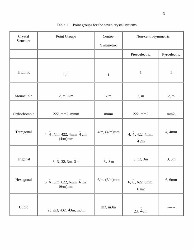
Table 1.1 Point groups for the seven crystal systems………….………………….………3
Table 1.2 Property differences between normal and relaxor ferroelectrics….….….……..9
Table 2.1 Some widely used electro-optic ferroelectrics…….….…...………….……….51
Table 3.1 Parameters from refractive index of PBN…………..…………………………70
Table 3.2 Parameters from birefringence of PBN …………….………………………...80
Table 3.3 Dielectric fitting results for PBN57……………………..…………………….89
Table 3.4 Slope of high temperature linear refractive index of PZT-0.12PT……..……103
Table 4.1 Thermo-optical coefficient of PBN at 535nm…………………………..…...114
Table 4.2 Thermo-optical coefficient of birefringence of PBN at high temperature…...114
Table 5.1 Optical energy gap and phonon energy of PZN-0.12PT……………….……128
Table 5.2 Parameters of PZN-0.12PT derived using Urbach rule………………..……132
x
List of Figures
Figure 1.1 Unit cells of the four phases of BaTiO3 as a function of temperature. (a) cubic
T>120°C (b) tetragonal 5°C <T<120°C, (c) orthorhombic -90°C <T<5°C, (d)
rhombohedral T<-90°C ……………………………………………………….6
Figure 1.2 A typical ferroelectrics hysteresis loop………………………….…………….7
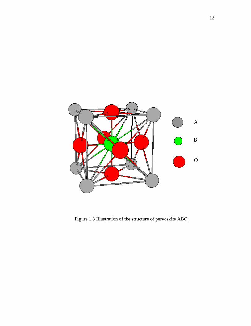
Figure 1.3 Illustration of the structure of pervoskite ABO3 ………………….………….12
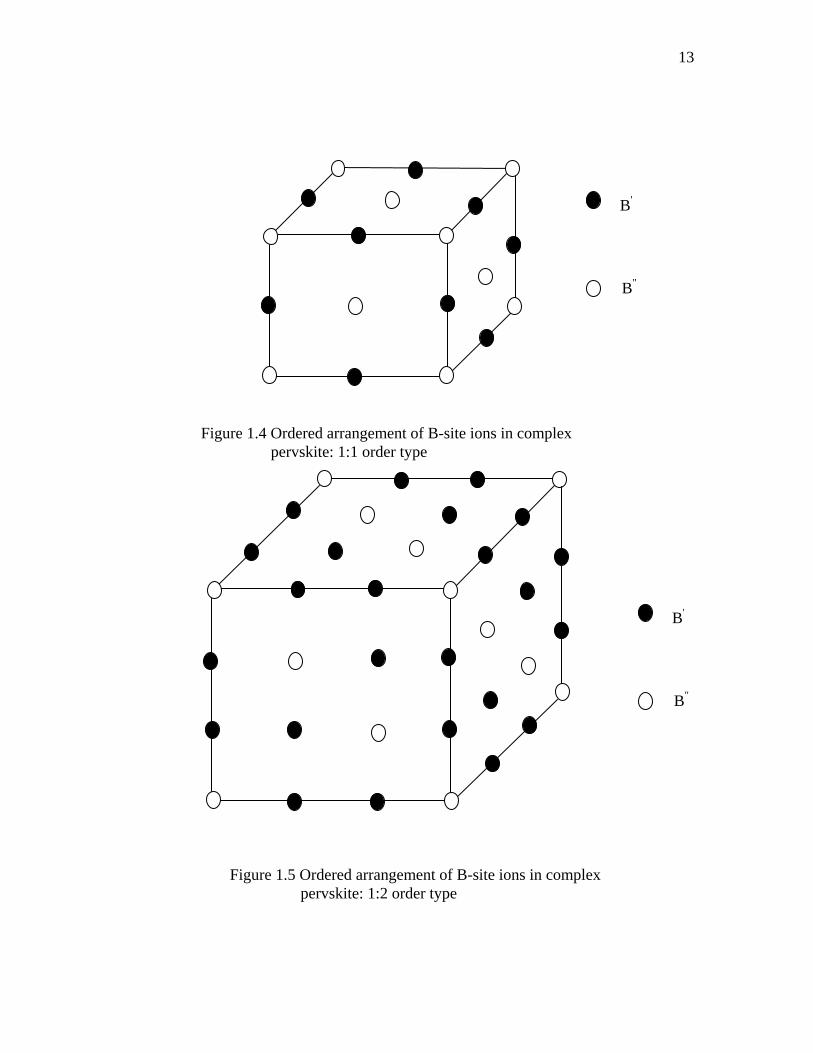
Figure 1.4 Ordered arrangement of B-site ions in complex pervskite: 1:1 order type.….13
Figure 1.5 Ordered arrangement of B-site ions in complex pervskite: 1:2 order type…...13
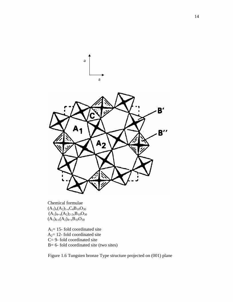
Figure 1.6 Tungsten bronze Type structure projected on (001) plane……………….…..14
Figure 1.7 Representation of the characteristic refractive index vs. temperature behavior
for ferroelectric systems with a) first order phase transition b) second order
phase transition c) a relaxor phase transition………………………….…….18
Figure 1.8 Basic domain structures of BaTiO3 in tetragonal phase. (a) and (b) are 90°
domain structures; (c) and (d) are 180° domain structures…………...……...21
Figure 1.9 The polar regions in the paraelectric environment…………………….……..29
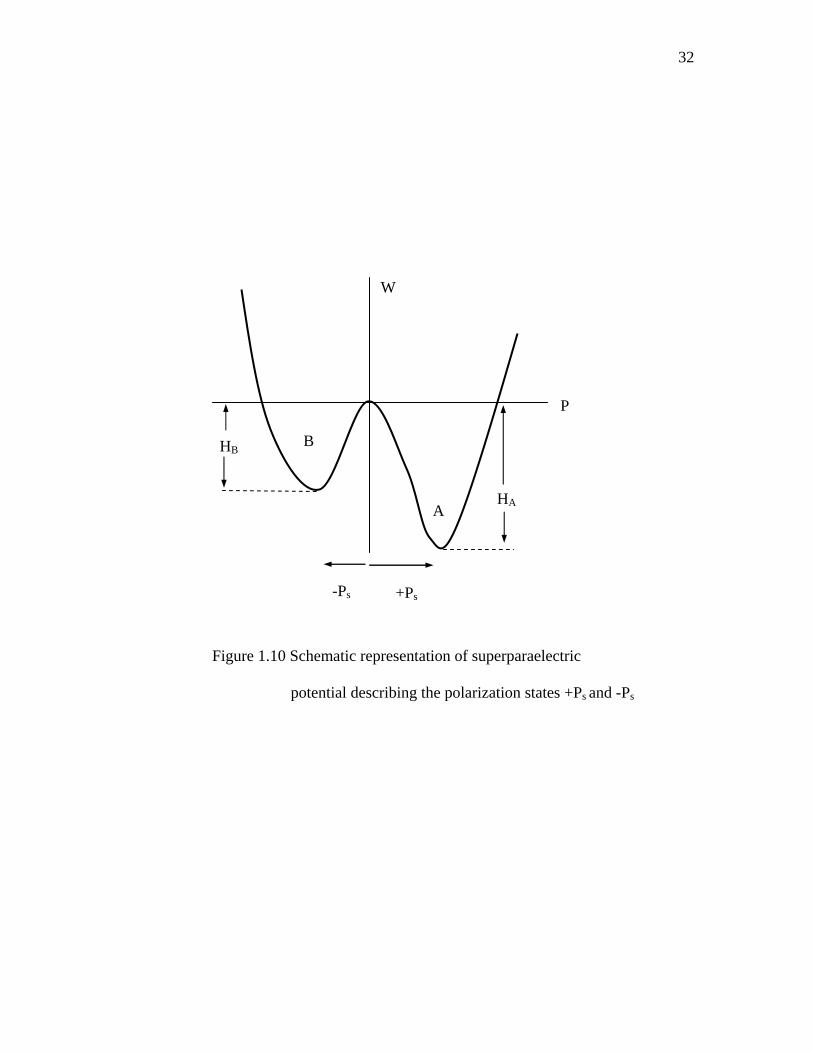
Figure 1.10 Schematic representation of superparaelectric potential describing the
polarization states +Psand -Ps …………………….……………………….32
Figure 1.11 Two type Transition (a) direct transition (b) indirection transition………....46
Figure 1.12 Theoretical curve of allowed indirection transition…….…….……………..47
Figure 3.1 Principle of minimum deviation measurement………………………….……57
xi
Figure 3.2 Measurement of minimum deviation angle………………………….……….57
Figure 3.3 Experiment setup of Birefringence measurement ………………….………..59
Figure 3.4 Wedge method for birefringence measurement……………………….……..60
Figure 3.5 Pseudobinary PBN morphtropic phase boundary diagram…………………..62
Figure 3.6 Optical refractive index n3 of PBN single crystal as a function of temperature
at λ=450, 535, 633, and 694nm……………………………….……….…..65
Figure 3.7 Single oscillator fitting for different temperature……………….……………66
Figure 3.8 Calculated energy of effective oscillator E0 vs temperature…….…………..67
Figure 3.9 Calculated dispersion energy Ed vs temperature………………….………….68
Figure 3.10 (a, b) Experimental and calculated refractive index of n3. The inclined lines
signify the trend of TD and Td , obtained by extrapolation guided by eye....69
Figure 3.11 Birefringence of PBN as a function of temperature at λ=535, 633, and
694nm……………………………………………………………………...78
Figure 3.12 Birefringence of PBN vs temperature with linear extrapolating of high
temperature intrinsic behavior, obtained by extrapolation guided by eye ...79
Figure 3.13 Calculated polarization of PBN as a function of temperature at λ=535, 633,
and 694nm ………………………………….……………….…….….……81
Figure 3.14 Summary of Ti, Td, TD, and Curie range of PBN as a function of
frequency…………………………………………………………………...82
Figure 3.15 g33 of PBN dispersion with temperature……………………..………….…..85
Figure 3.16 Corrected polarizations of PBN……………………………….……….……86
Figure 3.17 Dielectric constant and loss tangent of PBN57. a) heating run, b)cooling
run……………………………………………………………………….…90
xii
Figure 3.18 Dielectric constant and loss tangent of PBN57 at low temperature…….…...91
Figure 3.19 Phase diagram of PZN-PT around its MPB C:cubic, T: tetragonal, O:
orthorhombic, and R: rhombohedral………………………………..……..94
Figure 3.20 Optical refractive index n3 of PZN-0.12PT single crystal before poling as a
function of temperature at λ=450, 535, 633, and 694nm…………………..98
Figure 3.21 Optical refractive index n3 of PZN-0.12PT single crystal after poling as a
function of temperature at λ=450, 535, 633, and 694nm…………………..99
Figure 3.22 Temperature dependent effective dispersion oscillator energy E0….…..…100
Figure 3.23 Temperature dependent dispersion energy Ed………………………….….101
Figure 3.24 The ratio of effective dispersion oscillator energy E0 and dispersion energy
Ed (Epoled/Eunpoled)………………………….………………………………102
Figure 3.25 Birefringence of PZN-0.12PT as a function of temperature at λ=535, 633,
and 694nm…………………………………………………….…..………105
Figure 3.26 Polarization of PZN-0.12PT derived from refractive index as a function of
temperature for both poled and unpoled sample………….…...………….106
Figure 3.27 Polarization of PZN-0.12PT derived from birefringence as a function of
temperature at λ=535, 633, and 694nm…………………..…………..…..107
Figure 4.1 Thermo-optic coefficient of n3 of PBN…………………………………..…112
Figure 4.2 Thermo-optic coefficient of birefringence of PBN……………………...….113
Figure 4.3 Thermo-optic coefficient of n3 of unpoled PZN-0.12PT sample………….. 117
Figure 4.4 Thermo-optic coefficient of n3 of poled PZN-0.12PT sample…………...…118
Figure 4.5 Thermo-optic coefficient of birefringence of poled PZN-0.12PT sample….119
Figure 5.1 Transmission spectrums of PZN-12PT between 350-1000nm………….…..122
xiii
Figure 5.2 The transmission of light passing through sample with thickness of d….….124
Figure 5.3 Absorption coefficient of PZN-12PT in visible range………………..….…126
Figure 5.4 Allowed indirect transition accompanied by phonon in PZN-0.12PT……...127
Figure 5.5 Transmission spectrum fitted by Urbach rule…………………………..…..131
Figure 5.6 FTIR spectrum of PZN-0.12PT………………………………………..……136
Figure 5.7 Absorption peaks of PZN-0.12PT's FTIR spectrum………………….…….137
Figure 6.1 BaTiO3 with two domain I and II……………………………………….….140
Figure 6.2 90° domain wall between a-domain and c-domain………………………...140
Figure 6.3 90° domain wall between a-domains………………………………….…….143
Figure 6.4. Definition of coordinate system……………………………………………143
Figure 6.5 Light passing through two 90° domain……………………………….…….146 Figure 6.6 Schematic experiment setup………………………………………….……..149
Figure 6.7 Schematic arrangement of optical device…………………………….……..149
Figure 6.8 Optical performance of the voltage-controllable nematic liquid crystal retarder
at 632.8 nm…………………………………………………….…………152
Figure 6.9 Original 2-D intensity images captured by CCD with changing the rotation
angle of the analyzer……………………………………………...………156
Figure 6.10 Filtered 2-D intensity images for the different rotation angle of the
analyzer…………………………………………………………...………157
Figure 6.11 2-D profile of birefringence ),( θφ with applied voltage 3.23V….……….158
Figure 6.11 2-D profile of birefringence ),( θφ with applied voltage 3.99V …..….….159
Figure 7.1 Illustration of the coupling between light and polar regions at different
temperature ………………………………………………………………165
xiv
Acknowledgements
I would express my sincerely gratitude to my advisors Dr. Ruyan Guo and
Dr.Amar Bhalla for their guidance, support, and help during my study. Before I joined
this group about four years ago, I knew little about ferroelectrics and never thought I
could extend my academic career in this field. I would like to thank Dr. Guo and Dr.
Bhalla for their invaluable enlightenment and patience on my academic exploration. Also
I would like to thank the thesis committee members, Drs. Cross, White and Yin for their
time and insightful comments on this work.
This work cannot be finished without the help from my colleagues and the staff at
the MRL. They are: Dr Shujun Zhang Dr. Yoshi Somiya, Dr. Ed Alberta, Dr. Alok, Dr.
Chuanyong Huang, Dr. Youwei Fu, Mr. Hongbo Liu, Mr. Jeff Long, Mrs. Nicole
Wanderling, and Mrs. Man Gu.
Finally, my family in China deserves my profound gratitude for their support and
encouragement. Most of all, I would like to express my gratitude to my lovely wife
Hongli Pu.
1
Chapter 1 Introduction
1.1 Introduction of ferroelectrics
1.1.1 Ferroelectrics
Ferroelectricity is a phenomenon that was discovered in 1921. The name is
somewhat misleading as it is not related with iron despite the ferro- prefix. The
connection is as follows. Ferromagnetic materials have a spontaneous magnetization
below a critical temperature due to the alignment of magnetic dipoles and the prefix was
given because the first discovered compound contained iron. It is because of the analogy
between the magnetic and electric dipole behavior that ferroelectrics are named.
Ferroelectricity has also been called Seignette electricity, as Seignette or Rochelle
Salt (RS) was the first material found to show ferroelectric properties such as a
spontaneous polarization on cooling below the Curie point, ferroelectric domains and a
ferroelectric hysteresis loop.
Due to their typically high dielectrics constants and piezoelectric constants, a lot
of efforts in the research on ferroelectric materials came in the 1950's, leading to the
widespread use of barium titanate (BaTiO3) based ceramics in capacitor applications and
piezoelectric transducer devices. Since then, many other ferroelectric ceramics including
lead titanate (PbTiO3), lead zirconate titanate (PZT), lead lanthanum zirconate titanate
(PLZT), and relaxor ferroelectrics like lead magnesium niobate (PMN) have been
developed and utilized for a variety of applications. With the development of material
(ceramic) processing and thin film technology, many new applications have emerged.
The biggest use of ferroelectric ceramics have been in the areas such as dielectric
2
ceramics for capacitor applications, ferroelectric thin films for non volatile memories,
piezoelectric materials for medical ultrasound imaging and actuators, and electro-optic
materials for data storage and displays.
In the past few decades, many books and reviews have been written explaining
the concepts of ferroelectricity in materials [Lines and Glass 1977; Jaffe et al. 1971; Xu
1991]. In this chapter, an effort is made to introduce the basic principles governing
ferroelectricity and some general properties related to this thesis.
1.1.2 General Properties of Ferroelectrics
1.1.2.1 Crystal Symmetry
The lattice structure described by the Bravais unit cell of the crystal governs the
crystal symmetry. Though there are thousands of crystals in nature, they all can be
grouped together into 230 microscopic symmetry types or space groups based on the
symmetry elements [Nye 1990; Newnham 1975]. A combination of these symmetry
elements gives us the macroscopic symmetry also called as point groups. It can be shown
by the inspection of the 230 space groups that there are just 32 point groups. As shown in
Table 1.1, the seven crystal systems can be divided into these point groups according to
the point group symmetry they possess.
The thirty-two point groups can be further classified into (a) crystals having a
center of symmetry and (b) crystals which do not possess a center of symmetry. Crystals
with a center of symmetry include the 11 point groups labeled centrosymmetric in Table
1.1. These point groups do not show polarity. The remaining 21 point groups do not have
a center of symmetry (i.e. non-centrosymmetric). A crystal having no center of symmetry
3
Table 1.1 Point groups for the seven crystal systems
Crystal Structure
Point Groups Centro-
Symmetric
Non-centrosymmetric
Piezoelectric Pyroelectric
Triclinic
1, −
1
−
1
1
1
Monoclinic
2, m, 2/m
2/m
2, m
2, m
Orthorhombic
222, mm2, mmm
mmm
222, mm2
mm2,
Tetragonal
4, −
4 , 4/m, 422, 4mm, −
4 2m, (4/m)mm
4/m, (4/m)mm
4, −
4 , 422, 4mm, −
4 2m
4, 4mm
Trigonal
3, −
3 , 32, 3m, −
3 m
−
3 , −
3 m
3, 32, 3m
3, 3m
Hexagonal
6, −
6 , 6/m, 622, 6mm, −
6 m2, (6/m)mm
6/m, (6/m)mm
6, −
6 , 622, 6mm, −
6 m2
6, 6mm
Cubic
23, m3, 432, −
43m, m3m
m3, m3m
23, −
43m
------
4
possesses one or more crystallographically unique directional axes. All non-
centrosymmetric point groups, except the 432 point group, show piezoelectric effect
along unique directional axes. Piezoelectricity is the ability of certain crystalline
materials to develop an electrical charge proportional to a mechanical stress. It was
discovered by the Curie brothers in 1880. Piezoelectric materials also show a converse
effect, where a geometric strain (deformation) is produced on the application of a voltage.
The direct and converse piezoelectric effects can be expressed in tensor notation as,
jkijki dP σ= (1.1.1)
kkijij Ede = (1.1.2)
where Pi is the polarization generated along the i- axis in response to the applied stress
jkσ , and ijkd is the piezoelectric coefficient. For the converse effect, ije is the strain
generated in a particular orientation of the crystal on the application of electric field Ek
along the k-axis. [Lines and Glass 1977]
Out of the twenty point groups, which show the piezoelectric effect, ten point
groups (including 1, 2, m, mm2, 4, 4mm, 3, 3m, 6, and 6mm) have only one unique
directional axis. Such crystals are called polar crystals as they show spontaneous
polarization. Most of the non-vanishing properties of crystals can be derived from the
symmetry elements of unit cell or structure alone.
1.1.2.2 Phase transition
The characters of ferroelectrics exist only in a temperature range. Ferroelectricity
will disappear when temperature is higher than a phase transition temperature Tc, Curie
point. And the ferroelectrics transforms from ferroelectric phase to paraelectric phase,
5
with zero spontaneous polarization. The static dielectric constant obeys the Curie-Weiss
law:
0
0 TTC−
+= εε (1.1.3)
where 0ε is the dielectric constant of vacuum, C is the Curie constant and To is the Curie
temperature. For the second order transition cTT =0 while for first order phase transition
cTT <0 .
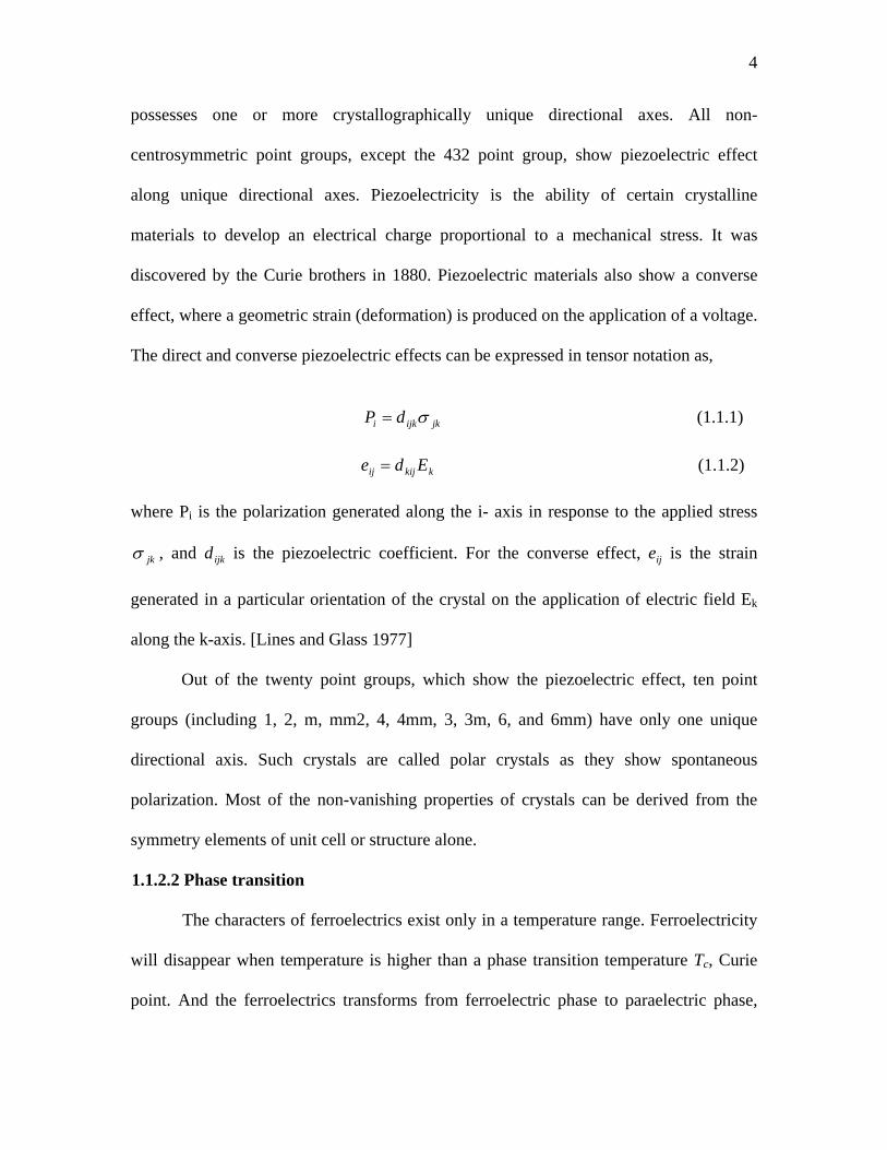
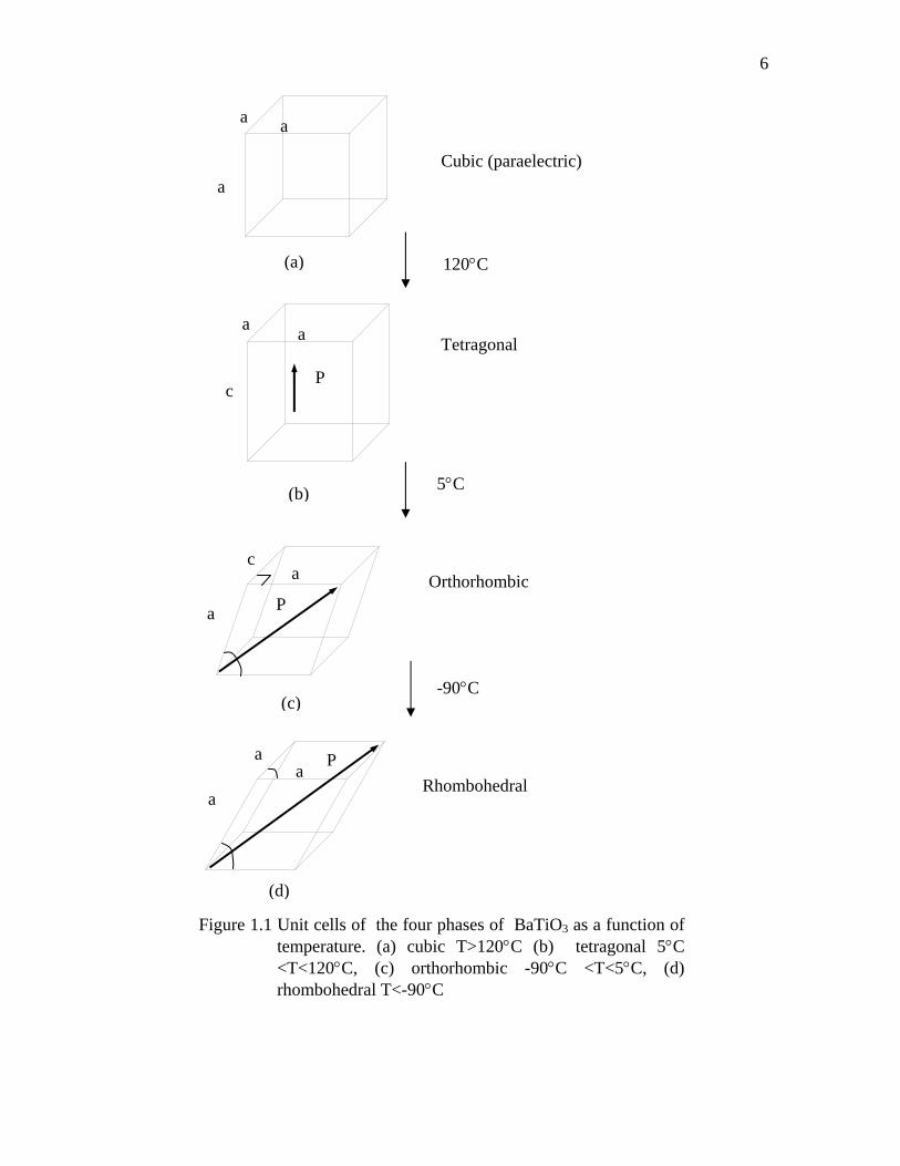
Ferroelectrics may exhibit one or more polar phase below Curie point. Barium
titanate (BaTiO3) has three polar phases as a function of temperature. Barium titanate
transforms from cubic (paraelectric) to tetragonal (ferroelectric) at 120°C, to
orthorhombic (ferroelectric) at ~5°C, and to rhombohedral (ferroelectric) at -90°C. The
polarization axes are along the [001], [110], and [111] directions for the tetragonal,
orthorhombic, and rhombohedral phase, respectively as shown in Figure 1.1.
1.1.2.3 Domain and hysteresis
When a ferroelectric crystal is cooled below the Curie temperature, in the
absence of external electric field and mechanical stress, it breaks up into domains of
different orientation under the constraints of boundary conditions. Within a domain, all
the electric dipoles are aligned in the same direction resulting uniform polarization. The
formation of the domains lowers the total energy of ferroelectrics. The polarization
direction in a domain can be switched to the direction of the electric field when the
ferroelectrics is in an applied electric field. The total polarization exhibits the
characteristic hysteresis loop when changing the magnitude and direction of the applied
6
a a
a
a a
c P
c a
a P
P a a
a
Cubic (paraelectric)
120°C
-90°C
5°C
Rhombohedral
Orthorhombic
Tetragonal
Figure 1.1 Unit cells of the four phases of BaTiO3 as a function of temperature. (a) cubic T>120°C (b) tetragonal 5°C <T<120°C, (c) orthorhombic -90°C <T<5°C, (d) rhombohedral T<-90°C
(a)
(c)
(d)
(b)
7
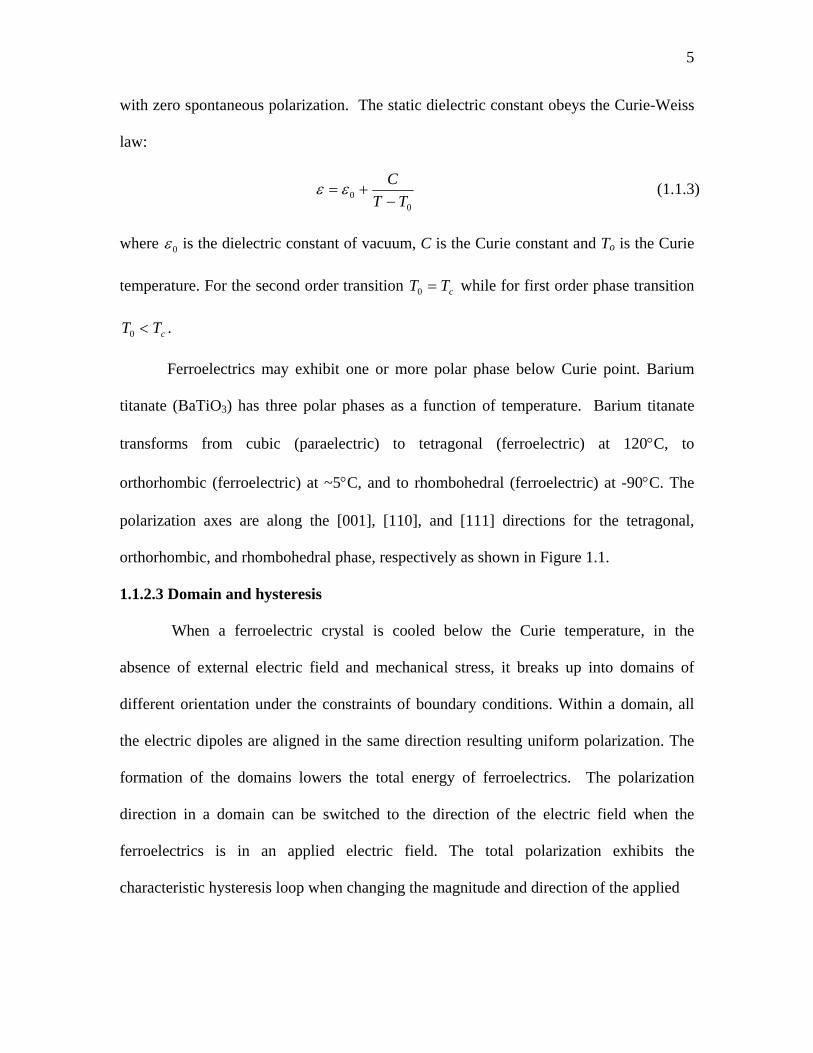
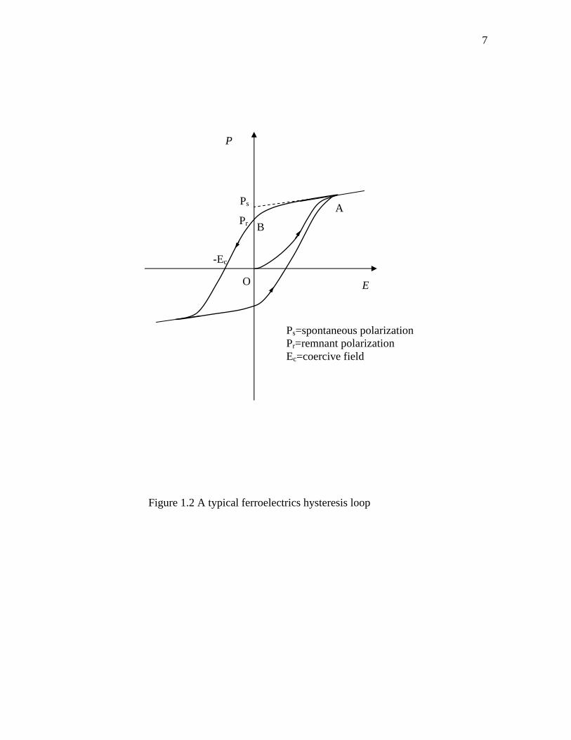
Ps=spontaneous polarization Pr=remnant polarization Ec=coercive field
Figure 1.2 A typical ferroelectrics hysteresis loop
Ps
P
E
-Ec
Pr
O
A
B
8
electric field as shown in Figure 1.2, assuming only two orientations of spontaneous
polarization in a ferroelectrics and the total polarization is zero in the absence of applied
electric field. Now applying an electric field along one orientation, the domains with the
polarization direction parallel to the electric field enlarge while the domains with the
polarization direction opposite to the electric field diminish. The total polarization
increases with the electric field corresponding to the curve OA in Figure 1.2. There is
only one domain in the ferroelectric when the electric field is strong enough. All
polarizations are parallel to the electric field and the total polarization is saturated. The
total polarization decreases to a remnant polarization Pr along the curve AB while the
electric field decreasing to zero. In order to remove the remnant polarization, a reversal
electric field > Ec (coercive field) is applied.
1.2 Relaxor ferroelectrics
Relaxor ferroelectrics are ferroelectrics with diffuse phase transitions, which are
characterized [Cross 1987] by (i) a significant frequency dependence of their peak
permittivity at Tm, (ii) persistence of the local polarization far above the phase transition
temperature TC , and (iii) absence of macroscopic spontaneous polarization and structural
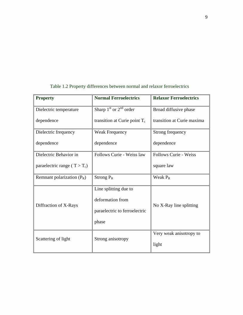
symmetry breaking after zero-field cooling. Table 1.2 listed the differences between the
normal and relaxor ferroelectrics. Some more explains will be given in later sections.
Relaxor ferroelectric behavior occurs dominantly in lead based perovskite
structures of A(B'B")O3 compositions, where B' is a low-valence cation (such as Mg2+,
Zn2+, Ni2+, Co2+, Fe3+, Sc3+, In3+, and Yb3+) and B" is a ferroelectrically active cation that
has a higher valence and no outer d-electron (such as Ti4+, Zr4+, Nb5+, Ta5+, and
W6+).[Glass 1969] Similar features are also observed in tungsten bronze
9
Table 1.2 Property differences between normal and relaxor ferroelectrics
Property Normal Ferroelectrics Relaxor Ferroelectrics
Dielectric temperature
dependence
Sharp 1st or 2nd order
transition at Curie point Tc
Broad diffusive phase
transition at Curie maxima
Dielectric frequency
dependence
Weak Frequency
dependence
Strong frequency
dependence
Dielectric Behavior in
paraelectric range ( T > Tc)
Follows Curie - Weiss law
Follows Curie - Weiss
square law
Remnant polarization (PR) Strong PR Weak PR
Diffraction of X-Rays
Line splitting due to
deformation from
paraelectric to ferroelectric
phase
No X-Ray line splitting
Scattering of light Strong anisotropy Very weak anisotropy to
light
10
structurematerials such as AxBa1-xNb2O6 (A=Sr, Pb) [Lines and Glass 1977]. First
discovered by Smolenskii et al. [Smolenskii and Isupov 1954], these materials exhibit
broad and anomalously large dielectric maximas which make them ideal candidate for
multilayer capacitors [Shrout and Halliyal 1987], electrostrictive actuators [Uchino
1986], pyroelectric bolometeters [Whatmore et al. 1987], electro-optics [McHenry et al.
1989], and for nonvolatile random access memories [Paz de Araujo et al. 1995]. The
existence of a morphotropic phase boundary in various solid solutions of relaxor
compounds with PbTiO3 (PT) similar to that in the well know Pb(Zr1-xTix)O3 (PZT)
system, also makes these materials excellent candidates for piezoelectric transducers
[Choi et al. 1989].
1.2.1 Structure of relaxor ferroelectric
Relaxor ferroelectrics behavior in crystalline ferroelectrics has been studied in
many ferroelectric solid solution systems, which have either the complex perovskite or
tungsten bronze crystal structure [Cross 1987, 1994].
1.2.1.1 Perovskite structure
Perovskite is a family name of a group of materials and the name comes from the
mineral CaTiO3 which exhibits a structure of type ABO3. Many normal ferroelectric
ceramics such as Barium Titanate (BaTiO3), Lead Titanate (PbTiO3), Lead Zirconate
Titanate (PZT), Lead Lanthanum Zirconate Titanate (PLZT), Lead Magnesium Niobate
(PMN), Potassium Niobate (KNbO3), have a perovskite type structure. Most perovskite-
type ferroelectrics are compounds with either A2+B4+O32-
or A1+B5+O32-
type formula.
The structure is illustrated in Figure 1.3.The A ions are the larger cations that sit
at the corners of the cube and is coordinated by 12 oxygen ions. The smaller B ions
11
occupy the center of the cube and surrounded by an oxygen octahedron. The oxygen
anions are situated at the center of the faces. Most ferroelectrics with oxide perovskite
structure are cubic at high temperature, but at low temperatures they may transform into
other structures. This structure is highly tolerant to cation substitution to A and B site
lattice, and lead to the complex perovskite structure A(B'B")O3. The structures of
A(B'1/2B"
1/2)O3 and A(B'1/3B"
2/3)O3 are illustrated in Figure 1.4 and 1.5, respectively. This
thesis will be concerned on solid solution of lead zinc niobate, Pb(Zn1/3Nb2/3)O3 with PT.
The single crystal Pb(Zn1/3Nb2/3)O3 (PZN) is a typical relaxor ferroelectric
material with globally disordered complex perovskite structure in which Zn2+ and Nb5+
cations exhibit only short order coherency (2-50nm) on the B site. The averaged
symmetry over the macroscopic scale is considered to be rohombohedral below the
diffuse phase transition temperature of about 140°C[Kuwata et al. 1981].
1.2.1.2 Tungsten bronze structure
Ferroelectric tungsten bronze structure (TB) is transparent in the visible range and
has tetragonal symmetry. The structure of the TB prototype is shown in Figure 1.6 as
projected in the (001) plane. The tetragonal unit cell consists of 10 BO6 octahedral linked
by their corners. In such a manner three different types of tunnels, i.e. square (A1),
pentagon (A2), and triangle (C), are formed parallel to the c-axis. There are two 12-fold
coordinated sites (A1), four 15-fold coordinated sites (A2), and four 9-fold coordinates
sites (C) per unit cell. The latter ones are the smallest. A large number of compound
crystallize with TB structure, but the variety, the size and charge of the metal cations can
12
A
B
O
Figure 1.3 Illustration of the structure of pervoskite ABO3
13
Figure 1.5 Ordered arrangement of B-site ions in complex pervskite: 1:2 order type
B'
B"
B'
B"
Figure 1.4 Ordered arrangement of B-site ions in complex pervskite: 1:1 order type
14
Chemical formulae (A1)x(A2)1-xC4B10O30 (A1)4+x(A2)2-2xB10O30 (A1)6-x(A2)4+xB10O30
A1= 15- fold coordinated site A2= 12- fold coordinated site C= 9- fold coordinated site B= 6- fold coordinated site (two sites) Figure 1.6 Tungsten bronze Type structure projected on (001) plane
a
a
15
cause subtle changes on the ferroelectrics phases and varying characteristics of
ferroelectric properties. For example, PbTa2O6 is orthorhombic both above and below Tc,
whereears PbNb2O6 is tetragonal above and orthorhombic below Tc, and Sr1-xBaxNb2O6
(SBN) remains tetragonal both above and below Tc [Lines and Glass 1977]. The general
composition may be considered to be close to one of the following formulae: (a)
(A1)x(A2)1-xC4B10O30 if both A1 and A2 are alkaline earth ions, (b) (A1)4+x(A2)2-2xB10O30if
A1 is an alkaline earth and A2 is an alkali, and (c) (A1)6-x(A2)4+xB10O30 if both A1 and A2
are alkali ions. This thesis also will be concerned on tungsten bronze PBN composition.
1.2.2 Dielectric and related electrical properties
The static dielectric constant of normal ferroelectrics exhibits a sharp, narrow
peak at Tc. For a single crystal the peak is very sharp and the width at half max is ~10–20
K. For a mixed oxide ferroelectrics the peak is somewhat rounded due to compositional
fluctuations, and the width at half max is typically ~20–40 K. The ferroelectric response
is frequency independent in the audio frequency range. By contrast a relaxor exhibits a
very broad )(Tε peak and strong frequency dispersion in the peak temperature Tm and in
the magnitude of ε below Tm. The conventional wisdom has been that the broad )(Tε
peak, also referred to as a "diffuse phase transition", is associated with compositional
fluctuations leading to many nano/micro polar regions with different compositions and
Tcs. The breadth of the peak is simply a manifestation of the dipolar glass-like response
of these materials.
The temperature dependence of )(Tε of a ferroelectric obeys a Curie–Weiss law,
above Tc by the linear 1/ ε versus T response. While )(Tε of a relaxor ferroelectrics
exhibits strong deviation from this law for temperatures of many tens to a few hundred
16
degrees above Tm. It is only at very high temperatures that a linear 1/ε versus T response
is obtained. Although the dielectric behavior of a typical relaxor is following the Curie -
Weiss square law. A more general dielectric behavior of relaxor ferroelectrics has the
form [ Kirilov and Isupov, 1973]:
α
ε)(1
mTT −∝ , (1.2.1)
where 21 ≤<α , diffuseness coefficient 2=α is a special case for the "complete"
relaxor ferroelectrics and 1=α for the normal ferroelectrics.
The P–E hysteresis loop is the signature of ferroelectrics in the low temperature
ferroelectric phase. The large remnant polarization, Pr is a manifestation of the
cooperative nature of the ferroelectric phenomenon. A relaxor, on the other hand, exhibits
a so-called slim loop. For sufficiently high electric fields the nano polar regions of the
relaxor can be oriented with the field leading to large polarization; however, on removing
the field most of these domains re-acquire their random orientations resulting in a small
Pr. The small Pr is evidence for the presence of some degree of cooperative freezing of
dipolar (or nano polar regions ) orientations.
The saturation and remnant polarizations of a ferroelectrics decrease with
increasing temperature and vanish at the ferroelectrics transition temperature Tc. The
vanishing of P at Tc is continuous for a second-order phase transition and discontinuous
for a first-order transition. No polar regions exist above Tc. By contrast, the field-induced
polarization of a relaxor decreases smoothly through the dynamic transition temperature
Tm and retains finite values to rather high temperatures due to the fact that nano polar
regions persist to well above Tm.
17
The ferroelectric transition can be thermodynamically first or second order and
involves a macroscopic symmetry change at Tc. Transparent ferroelectrics exhibit strong
optical anisotropy across Tc. However, there is no structural phase transition across Tm in
a relaxor. The peak in )(Tε is simply a manifestation of the slowing down of the dipolar
motion below Tm. For transparent relaxors, there is no optical anisotropy across Tm.
1.2.3 Optical properties
The influence of phase transitions on the temperature dependence of refractive
indices of transparent materials (whether they are structural, magnetic, soft-mode, normal
ferroelectric or related to this work, relaxor ferroelectrics) has attracted growing interest
[Schafer and Kleemann 1985]. Refractometry in the precursor region of ferroelectric
phase transitions in the order to obtain information on the order parameter fluctuations
above the Curie temperature has grown in importance as a means of probing the onset of
the local short range order of polarization clusters [Burns and Dacol 1990a,b].
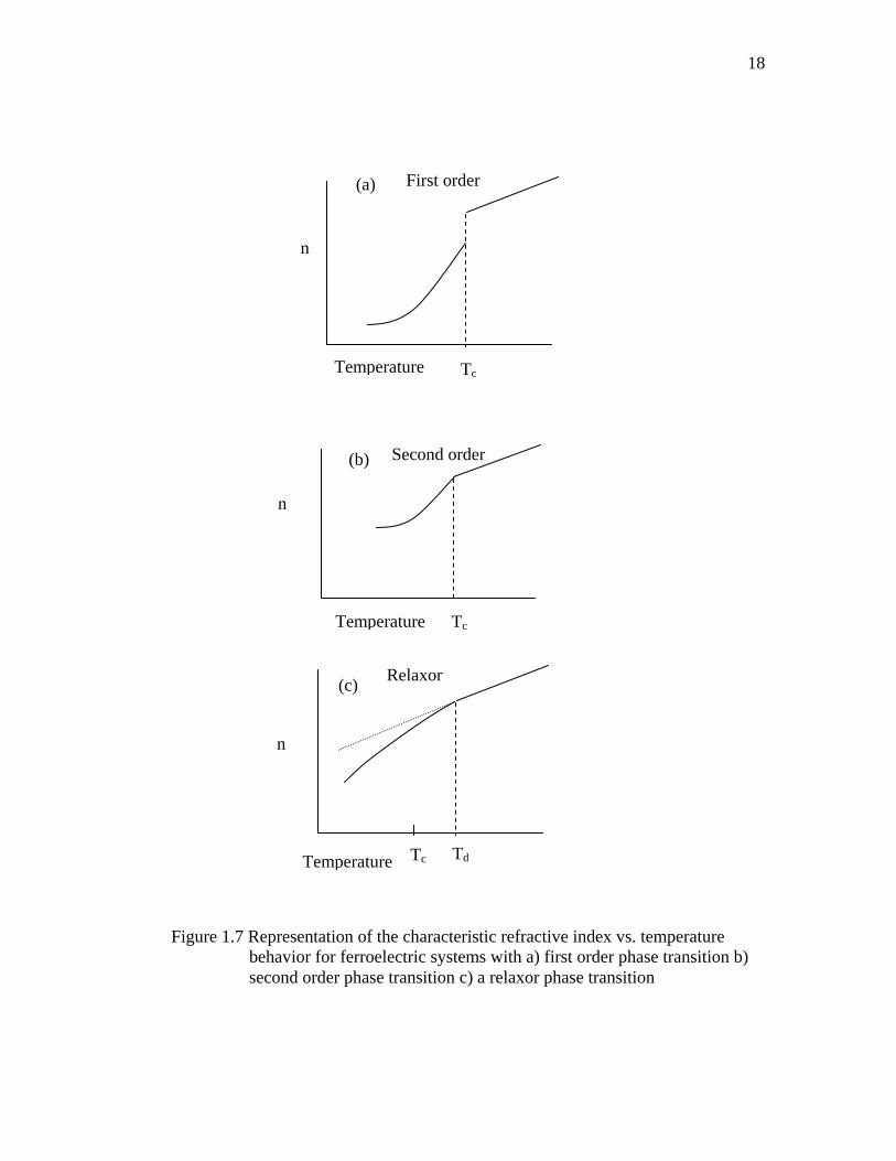
The characteristic refractive index behavior of three types of ferroelectric phase transition
is illustrated in Figure 1.7 for a normal first order ferroelectric phase transition, a second
order transition, and a relaxor ferroelectric. For a normal ferroelectric phase transition,
the refractive index is linear at high temperature and then at Tc abruptly departs from
linear behavior with a sharp discontinuity for a first order transition, or with a change in
slope at a second order transition. In contrast, relaxor ferroelectrics display quite different
behavior. At a temperature well above Tm the n(T) curve for relaxor departs from the
straight line high temperature regimes and gradually becomes nonlinear. This
temperature is referred to as a dipolar or Burns temperature.
18
(a)
Temperature
n
Tc
First order
(c)
Temperature
n
Td Tc
Relaxor
(b)
Temperature
n
Tc
Second order
Figure 1.7 Representation of the characteristic refractive index vs. temperature behavior for ferroelectric systems with a) first order phase transition b) second order phase transition c) a relaxor phase transition
19
1.3 Domain in ferroelectrics
1.3.1 Ferroelectric Domain
Besides the fundamental importance to understand the relaxor ferroelectrics,
domain investigation is also motivated by some practical applications, such as the general
trend of miniaturization of electronic devices, photonic devices and nonvolatile random
access memories.
When a ferroelectric crystal is cooled below the Curie temperature, in the absence
of external electric field and mechanical stress, it breaks up into domains of different
orientation under the constraints of symmetry requirement and boundary conditions. The
main contributions to the free energy that can be reduced or increased by the formation of
domain are: (i) the electrostatic energy or the depolarization energy, (ii) the energy of
certain strain fields around imperfections, (iii) the domain wall energy, and (iv) the
elastic energy. Therefore, if the crystal is brought to the ferroelectric state from the
paraelectric phase by decreasing temperature, the minimization of the total system free
energy may result in multi-domain structure. In addition, the distribution of internal stress
due to crystal defects is considered to give rise to multi-domain structures. Qualitatively,
to reduce the depolarization energy, antiparallel (180°) domains are favored. To decrease
the strain energy, 90° domain (or other permissible non-90° domain walls) would be
favored. If the spontaneous strain is small, forming 90° domains will not significantly
reduce energy, thus one finds the crystal stays single domain or form 180° domains. If the
crystal contains enough free mobile charge carriers that can sufficiently screen the
depolarization field, 180° domain may not form and crystal may stay single domain.
20
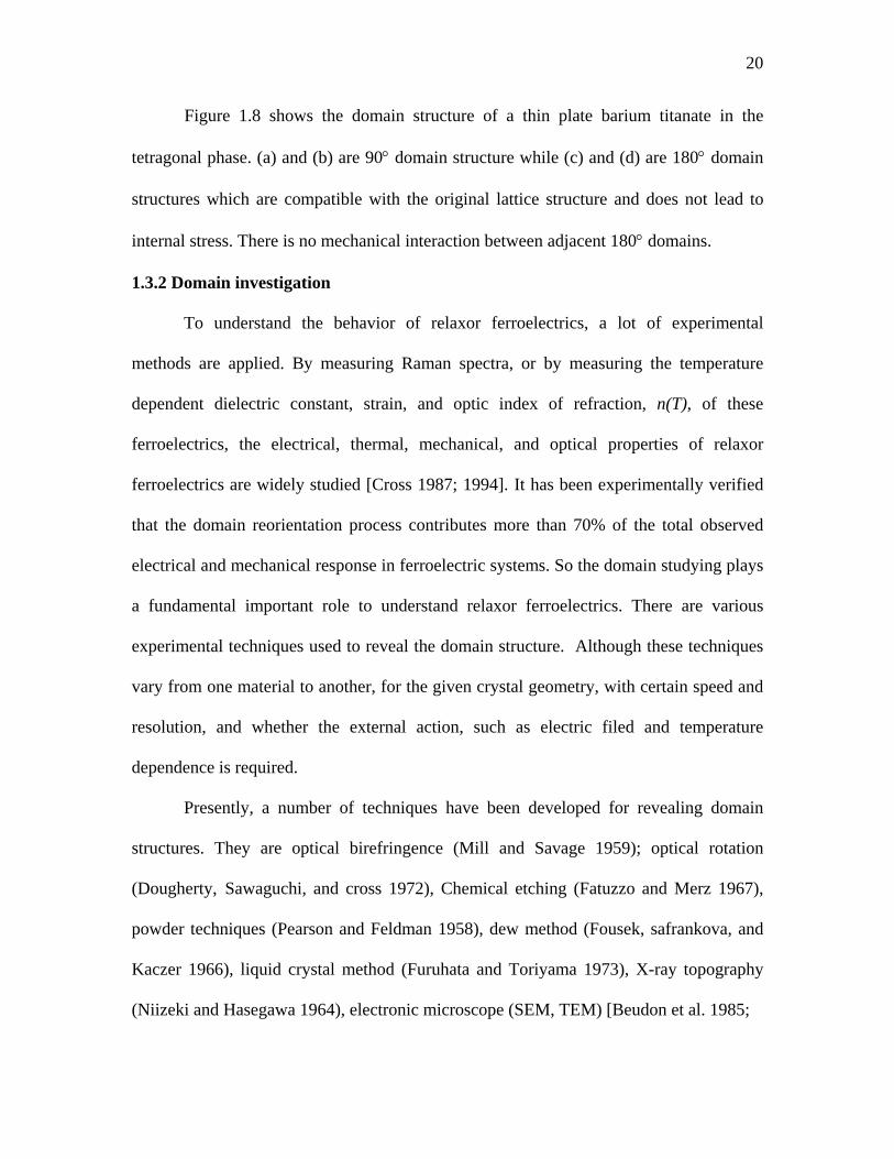
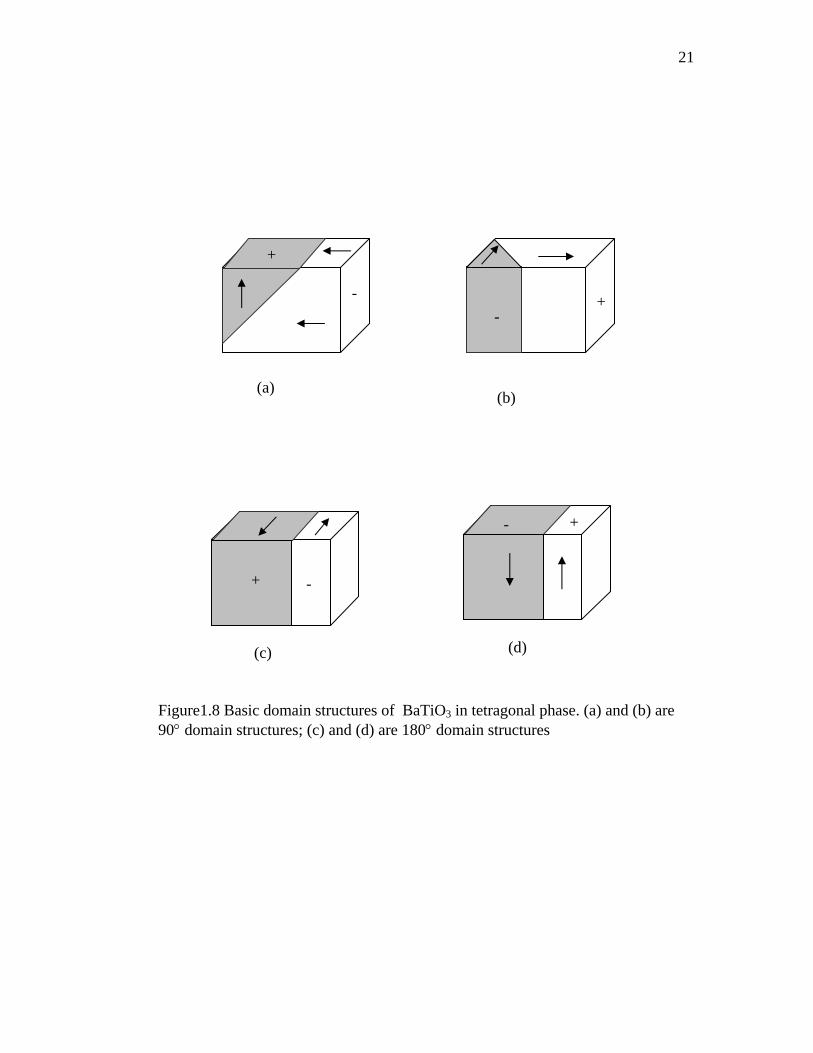
Figure 1.8 shows the domain structure of a thin plate barium titanate in the
tetragonal phase. (a) and (b) are 90° domain structure while (c) and (d) are 180° domain
structures which are compatible with the original lattice structure and does not lead to
internal stress. There is no mechanical interaction between adjacent 180° domains.
1.3.2 Domain investigation
To understand the behavior of relaxor ferroelectrics, a lot of experimental
methods are applied. By measuring Raman spectra, or by measuring the temperature
dependent dielectric constant, strain, and optic index of refraction, n(T), of these
ferroelectrics, the electrical, thermal, mechanical, and optical properties of relaxor
ferroelectrics are widely studied [Cross 1987; 1994]. It has been experimentally verified
that the domain reorientation process contributes more than 70% of the total observed
electrical and mechanical response in ferroelectric systems. So the domain studying plays
a fundamental important role to understand relaxor ferroelectrics. There are various
experimental techniques used to reveal the domain structure. Although these techniques
vary from one material to another, for the given crystal geometry, with certain speed and
resolution, and whether the external action, such as electric filed and temperature
dependence is required.
Presently, a number of techniques have been developed for revealing domain
structures. They are optical birefringence (Mill and Savage 1959); optical rotation
(Dougherty, Sawaguchi, and cross 1972), Chemical etching (Fatuzzo and Merz 1967),
powder techniques (Pearson and Feldman 1958), dew method (Fousek, safrankova, and
Kaczer 1966), liquid crystal method (Furuhata and Toriyama 1973), X-ray topography
(Niizeki and Hasegawa 1964), electronic microscope (SEM, TEM) [Beudon et al. 1985;
21
+
- + -
+ -
+ -
(a) (b)
(c) (d)
Figure1.8 Basic domain structures of BaTiO3 in tetragonal phase. (a) and (b) are 90° domain structures; (c) and (d) are 180° domain structures
22
Hilczer and Szezesniak 1989], AFM [Haefke 1994], and so on. Optical refractive index
measurement approach maybe the very convenient in-situ observation technique among
these techniques.
Lithium niobate (LiNbO3), lead zirconate titanate (Pb(Zn1/3Ti2/3)O3, PZT), lead
zirconate Niobate (Pb(Zn1/3Nb2/3)O3 ,PZN), and the mixture of lead titanate (PT) and PZT
are the most intensively investigated solutions.
Precise control of ferroelectric domains is a very important issue for many
applications, most notably, the periodical poling of materials LiNbO3, which are the basis
for many powerful nonlinear optical devices, such as optical amplifiers and parametric
oscillators. This makes the LiNbO3 intensively investigated material [Gopalan 1998].
PZT thin film has great potential to be an ultrahigh density (100G bit/cm2 class)
medium for scanning probe microscopy-based data storages [Hidaka et al. 1996]. It is
also of great benefit for the domain switching study of PZT since the domain structure
will be quite simple if the orientation of the PZT thin film can be controlled along the c-
axis orientation. Atomic force microscopy (AFM) and scanning force microscopy (SFM)
[Gruverman et al. 1998], a generalization of AFM is usually used to study and control the
local domain behaviors for their ultrahigh resolution compared with conventional
techniques. Switching and backswitching, the polarization reversal in the absence of
electric field, are two key issues in ferroelectric memories [Fu 2003]. Hidaka et al.
[Hidaka et al. 1996] has successfully written and imaged polarized domains with a size of
40-50 nm using an AFM technique. The mechanism of backswitching, which is critical to
understand the origin of polarization retention loss in ferroelectric memory, is still not
clear.
23
PZN is known as a relaxor ferroelectric with a broad, large dielectric constant and
high electromechanical coupling constant, which makes it and its mixture system (1-x)
PZN-xPT, potential for applications in actuators and transducer [Kuwata 1979]. Since the
domain reorientation mechanism contributes to the dielectric and piezoelectric properties,
it is important to understand the domain reorientation so that the actuators and transducer
properties can be tailored [Mulvihill 1995; Iwata et al. 2002]. Optical method is used
since it is convenient to apply electric field and to vary temperature to study the dynamic
ferroelectric domains and meanwhile making the in-situ observation also.
1.3.3 Size effect
The study of size effect on ferroelectrics has been an interesting subject both in
experiment and theory. Experimental studies have reported two critical grain sizes, which
have a major influence on ferroelectricity.
The first one, which occurs in the submicro size range, is characterized by a
transition from multidomain to single domain grains. This transition was found to be at a
critical grain size of about 200nm in PbTiO3 thin films [Lu 1996], 100nm in BaTiO3
powder particles [Hasiang and Yen 1996], and 300nm in PbZr0.95Ti0.05O3 crystallites
[Tuttle 1999]. The critical size was predicted theoretically by minimizing the total energy
of the structure [Zhong 2001].
The second critical grain size refers to the disappearance of ferroelectric
behaviors. Experimental studies have reported a critical size in the nanometer range, such
as 49nm for BaTiO3 thin films [Schlag and Eicke 1994], 30nm for BaTiO3 powder
particles [Hasiang and Yen 1996], and 7-14nm for PbTiO3 thin films [Chattopanhuay
1995]. Studies of single-crystalline PbZr0.25Ti0.75O3 thin films reported a local
24
ferroelectric reponse from a film thickness as small as 4 nm, a thickness of 10 unit cells
[Tybell 1999] using piezoelectric and electric-field microscope. Theoretical models have
been developed to calculate and predict this critical size. The models are maybe identified
in three categories. One is thermodynamic model, which is under the frame of Landau-
Devonshire’s theory [Scott 1988]. This model based on mean-field assumption, predicts a
material dependent critical size by minimizing the free energy of the finite crystallite and
taking into account the contribution of volume and surface terms. Secondly, the model
[Ghosez and K. M. Rabe 2000] is based on first-principle calculations, predicts
ferroelectric behaviors in ultrathin PbTiO3 films with a thickness as low as three unit cell.
Another model [Zhong 1994] is originated from Ising model in a transverse field, taking
into account surface effect and effects of depolarization fields among others. Recently
Koray et al. [ Akdogan 2002] proposed a phenomenological theory of size effects on the
Cubic-Tetragonal phase transition in BaTiO3 nanocrystals, which considered sized effects
as an intrinsic phenomenon on the basis of size dependent spontaneous polarization and
strains.
It’s evident that grain size plays a role in the phase transition. Can this size effect
be probed by optical method; say the light with different frequency may have different
interactions with the same size grain? With this basis, the optical interaction with the
nano/microregion in relaxor is also under the thesis’s scope.
1.4 Review of the various models of relaxor ferroelectrics There are various theories proposed to understanding the behaviors of relaxor
ferroelectrics materials. Usually some of the properties can be explained by each theory.
25
None of them can describe all the properties. Moreover, these theories sometimes
contradict with each other.
1.4.1 First principles calculation
There are still lots of unsolved questions for researchers who are exploring the
origin of ferroelectricity, such as, why SrTiO3 is not ferroelectrics while BaTiO3 and
PbTiO3 are ferroelectrics although they have the same structure and chemical properties
[King-Smith 1994]. Maybe the final answer can be found by means of the first principles
calculation. This was extremely difficult about twenty years ago. The understanding of
ferroelectrics with first principles has been significantly advanced in the last ten years
with the development of electron density function and the application of powerful high-
speed computer [Wu 2003].
First principles calculation starts from the fundamental interactions among
electrons and nuclei, not from the experimental data used as constrain parameters. Solid
is considered as a multi-particle system consisting of electrons and nuclei. The total
energy of the system is calculated by solving the Schrödinger equation. The system state
is then determined by the total energy and the electronic structure. Comparing with soft-
mode theory, concerning the movement of ions but omitting the contribution of electrons
by the adiabatic approximation, first principles emphasized the contribution of electrons,
the medium between ions' interaction.
Most of the first principles methods applied to ferroelectric are based on density
functional theory (DFT) and some are based on Hartree-Fock theory . The DFT states
that the ground state properties of a system are given by the charge density using an
effective exchange-correlation potential (Vxc) that accounts for electron interaction from
26
the view point of quantum mechanics. The main difficulty within DFT is how to treat the
exchange-correlation potential since the exact form of it remains unknown. The local
density approximation (LDA) takes the exchange-correlation potential from the uniform
electron gas at the density for each point in the material. Two classes of methods usually
used to solve to LDA equation are pseudopotential method and all-electron method. The
LDA predicts many properties of ferroelectrics, such as phonon frequencies, ferroelectric
transitions, polarization, and elasticity etc [Cohen 1999]. The generalized gradient
approximation (GGA) including the effect of local density gradient in the density, tends
to improve upon LDA in many aspect, such as atomic energies and structural energy
differences.
Weyrich et al. [Weyrich 1990] calculated the electronic structure and total energy
of BaTiO3. Their calculation indicated that any lattice distortion lowering symmetry
would change the non-overlap electronic state to overlap state. Calculated total energy
supported that the different behavior of BaTiO3 and SrTiO3 is due to the volume effect.
Cohen[Cohen 1990] showed that there was an overlap between electron wave
functions of Ti 3d and O 2p, and the overlap was enhanced by ferrodistortion, by
calculating the densities of state in valence band of BaTiO3 and PbTiO3. This is agreed
with Weyrich's [Weyrich 1990] result. Cohen also suggested that hybridization between
Ti 3d and O 2p was necessary to exhibit ferroelecticity for ABO3 perovskite ferroelectrics.
It is the hybridization between Ti 3d and O 2p that reduces or balances the short-range
repulsions, which tend to stabilize crystals with respect to off-center displacement.
Using an effective Hamiltonian and Monte carlo method, Garcia and Vanderbilt
[Garcia 1998] studied piezoelectric response of BaTiO3 as a function of applied field and
27
temperature. They obtained good agreement with the temperature dependence of
piezoelectric constants, and found a field induced rhombohedral to tetragonal phase
transition at very large fields. Rabe and Cockayne [Rabe 1998] used an effective
Hamiltonian for PbTiO3 and calculated piezoelectric constant d33 as a function of
temperature using Monte Carlo, also finding good agreement with the experimental
temperature dependence, which peak strong at the ferroelectric phase transition.
It will be a challenge to apply these methods to compute relaxor system, but
models can be parameterized using first principles results and Monte Carlo simulation
could be used to simulate rather small disorder system. To simulate much larger,
mesoscopic system, it maybe necessary to parameterize models for interactions between
nanoregions, leaving the atomic domains all together.
1.4.2 Compositional fluctuation model theory
One of the earliest accepted models for the understanding of relaxor
ferroelectrics proposed by Smolenskii and Isupov [Smolenskii and Isupov 1954] and
advanced by Isupov [Isupov 2003] continuously was based on compositional fluctuations.
This model suggested that ferroelectric relaxors have a common characteristic of two or
more cations occupying equivalent crystallographic sites in the lattice structure. These
fluctuations could result in different local Curie temperature (TC,loc), where the polar
nanoregions in the order of ~10nm are formed, in microregions due to the dependence of
the Curie temperature on the concentration of the components. These microregions are
large enough to allow the occurrence of spontaneous polarization Ps in it in the absence of
Ps in the surroundings. Polar nanoregions with different TC,loc, sizes, dipole moments,
spontaneous deformations and activation energies of depolarization, are distributed
28
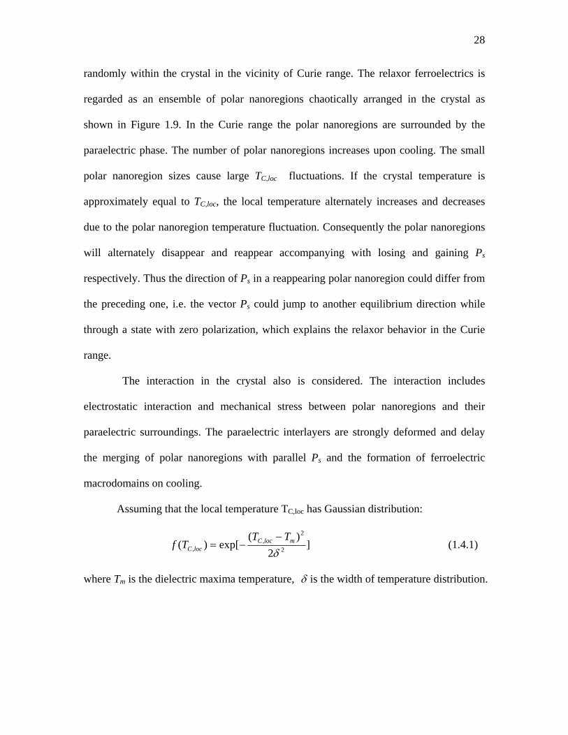
randomly within the crystal in the vicinity of Curie range. The relaxor ferroelectrics is
regarded as an ensemble of polar nanoregions chaotically arranged in the crystal as
shown in Figure 1.9. In the Curie range the polar nanoregions are surrounded by the
paraelectric phase. The number of polar nanoregions increases upon cooling. The small
polar nanoregion sizes cause large TC,loc fluctuations. If the crystal temperature is
approximately equal to TC,loc, the local temperature alternately increases and decreases
due to the polar nanoregion temperature fluctuation. Consequently the polar nanoregions
will alternately disappear and reappear accompanying with losing and gaining Ps
respectively. Thus the direction of Ps in a reappearing polar nanoregion could differ from
the preceding one, i.e. the vector Ps could jump to another equilibrium direction while
through a state with zero polarization, which explains the relaxor behavior in the Curie
range.
The interaction in the crystal also is considered. The interaction includes
electrostatic interaction and mechanical stress between polar nanoregions and their
paraelectric surroundings. The paraelectric interlayers are strongly deformed and delay
the merging of polar nanoregions with parallel Ps and the formation of ferroelectric
macrodomains on cooling.
Assuming that the local temperature TC,loc has Gaussian distribution:
]2
)(exp[)( 2
2,
, δmlocC
locC
TTTf
−−= (1.4.1)
where Tm is the dielectric maxima temperature, δ is the width of temperature distribution.
29
Figure 1.9 The polar regions in the paraelectric environment (from [Isupov 2003]
30
∫
∫∞
∞
=
0 ,,
0 ,,,
)(
)(),(
1
)(1
locClocC
locClocClocC
dTTf
dTTfTT
Tε
ε (1.4.2)
Assuming that the phase transition of polar nanoregion is of first order and Curie-
Weiss law is hold for )( ,locCTε , i.e.
locCm
locCmlocC
mmm
locCr TTC
TT
TTTT
TTTTc
TTC
T,
,2/1
,
, ,
},])(4
)(31[1){(316)(4
{)(
1
>−
<−
−−+−+−−
=ε
(1.4.3)
Considering two extreme cases:
(i) mTT −>>δ , corresponding to high degree of diffuse phase transition:
]2
)(exp[1)(
12
2
δεεm
rmr
TTT
−−= . (1.4.4)
Expanding the exponent into a power series in terms of mTT − and dropping the
higher order terms.
2
2
2)(1
)(1
δεεε rm
m
rmr
TTT
−=− (1.4.5)
This is the Curie - Weiss square law, which holds for relaxor ferroelectrics.
(ii) mTT −<<δ , corresponding to low degree of diffuse phase transition:
mr
TTT
−∝)(
1ε
(1.4.6)
This is the Curie - Weiss law, which holds for normal ferroelectrics.
This model gives the most direct explanation of the broad diffuse phase transition
by the existence of polar nanoregions, generally accepting by other models. The
weaknesses [Randall and Bhalla, 1990a]of this model are as follows:
31
(i) It can not make a distinction between compounds and solid solutions with
mixed cation sites and also their tendency to exhibit normal or relaxor behavior; or why
so many nonrelaxor ferroelectrics have a diffuse phase transition.
(ii) Localization of polar nanoregions requires enough gradient of chemical
composition, this is controversial with the Gaussian distribution assumption about the
local temperature, resulting fine variations in chemical composition through the crystal.
1.4.3 Superparaelectricity model theory
A theory proposed by Cross [Cross 1987] in analogy with superparamagntic
cluster materials is based upon the view that polarization clusters exist metastably or in
terms of kinetic disordering. The alternative polarization states, +P and –P, which are
superparaelectric potentials of a polar cluster (comparing with Isupov's term 'polar region',
here using 'polar clusters'), are separated by an activation barrier as illustrated in Figure
1.10. The height of the barrier H is proportional to the volume V of the polar region itself.
Due to the composition heterogeneity the composition gradient would not be identical
along these two opposite directions, thus the two potential wells have different depth. For
low thermal energies the polarization will lock-in to a particular orientation and form a
polar microdomain or cluster. Apparently the lower well A has the priority for polar
cluster to stay. However, the polar orientation can be perturbed from the lower well A,
which would lead to dispersion in dielectric response. A flipping of the polarization
orientation from one state to another state could happen for sufficient thermal energy.
The flipping frequencyν is given by:
))(exp(TkVH
BD −=νν . (1.4.7)
32
+Ps -Ps
HA
Figure 1.10 Schematic representation of superparaelectric
potential describing the polarization states +Ps and -Ps
B
A
HB
P
W
33
where Dν is Debye frequency (~1011-1013Hz), Bk is Boltzman constant. Since BA HH > ,
one can expect that the polar region will stay in well A longer, i.e. +Ps has longer "show
time". Isupov [Isupov 1999] obtained preexponential factor HzD4010~ν , activation
energy eVVH 7~)( , both of which are physically unrealistic for simple thermally
activated polarization fluctuation. However, by extrapolating Cole-Cole plots Isupov
obtained activation energy on the order of kBT with a preexponential factor of 109 Hz. He
ascribed the dielectric relaxation to temperature dependence of the number of polar
regions.
With the analogy with magnetization behavior in superparamagnetic material, the
polarization of an ensemble of uniform noninteracting polar regions having uniaxial
symmetry can be described by:
)tanh(Tk
EPpB
= (1.4.8)
where p is the reduced or normalized polarization, E, the electric field, P, the dipole
moment of the polar region. If p at different temperature is plotted against E/T (rather
than E), all the curve should superimpose on one another. The implication of the
superposition is that at higher temperature it takes much more electrical energy to align
the moments against the thermal energy.
The superparaelectric model, without incorporating the coupling between polar
regions, accurately describes many of the observed properties of ferroelectric relaxors
such as the frequency dependence of the permittivity, dielectric aging, metastable
switching from micro to macro domain states, and the nonlinear behavior of the
thermoelastic and optical properties [Cross, 1987].
34
The nanoscale order domains act as natural site to localize the high temperature
superparaelectric polar clusters within a paraelectric matrix on a scale of ~10nm. This is
consistent with the size of polar nanregion in Isupov's model. So here polar cluster is
exactly the polar nanoregion. So the broad diffuse phase transition also ascribed to the
size distribution of the polar clusters.
One advantage of this model over compositional fluctuation model is that the
scale of B-site order allows distinguishing whether a material will exhibit normal or
realxor ferroelectric behavior.
1.4.4 Dipolar glass model
The dipolar glass phase is characterized by two temperatures, Td, Burns
temperature (or dipole temperature) [Burn, 1985], and Tf [Viehlandet al, 1990b], freezing
temperature. The relaxors exhibits glassy behavior between these two characterization
temperatures. However, these two characterization temperatures are from different
evidence. It is interesting to put them together, although they are proposed independently.
Burns and Dacol [Burn, 1985; Burns et al., 1983a,b, 1985, 1986, 1990a, b, c]
made comprehensive study on materials with both complex perovskite structure and
tungsten bronze structure by accurate measurement of optical refractive index, thermal
expansion, and Raman spectrum. They found that up to hundreds degrees above Tm,
where the index deviates from a high temperature linear behavior, a local random
polarization (or glassy dipolar) still exist in the relaxor system. In the temperature range
from Tm to Td, the average polarization _P is zero, but the root mean square polarization
2/1_
2 )(P is not zero.
35
Burns and Dacol’s [Burns, 1985] the idea of composition fluctuations is
transformed. From their experiment fact that Td , the dipole temperature, is approximately
the same as the Tc of the end member, AB'O3 of the mixed system A(B'B")O3, they
concluded that in mixed system A(B'B")O3 the local polarization begins to appear at the
temperature Td>> Tm in the region containing only B' (but not B") ions. The idea of
composition fluctuations is transformed. From their experiment fact that Td , the dipole
temperature, is approximately the same as the Tc of the end member, AB'O3 of the mixed
system A(B'B")O3, they concluded that in mixed system A(B'B")O3 the local polarization
begins to appear at the temperature Td>> Tm in the region containing only B' (but not B")
ions. One can infer that the polar region must be very small and only containing several
unit cells (~1nm). However, this is contradictory to Smolenskii’s model that the polar
region can not be smaller than a critic size (~10nm).
The superparaelectric model was extended by Viehland et al. [Viehland et al.,
1990a, 1990b, 1991] as dipolar glass models to account for polar cluster interaction in
analogy to magnetic spin glass. By fitting the frequency and temperature dependent
dielectric constants with Vogel-Fulcher relation
)exp(0fm
a
TTEff−
−= (1.4.9)
where Tf is the static freezing temperature, Ea the activation energy, f0 the Debye
frequency. The extrapolated values of freezing temperature usually are very close to
temperature of the collapse in the remnant polarization [Viehland et al., 1990b]. The
fundamental difference between glassy dipole freezing and thermal localization process
in superparaelectrics is that freezing is a cooperative performance while the thermal
localization is an independent behavior. This cooperative performance is believed to be
36
an indication of interactions between polar regions. The local field of a polar region has
the tendency to polarize its neighboring polar regions over a correlation radius. Neutron
scattering experiments [La-Orauttapong,et al, 1999] reveals that this correlation radius is
temperature dependent.
These models successfully explained the polar dynamics and their extreme
slowing down at the diffuse phase transition. However, they are not capable of describing
the ferroelectric symmetry breakdown on a nanometric scale [Mathan,et al, 1991]. The
Vogel-Fuclcher relation is not the only one that can describe the frequency and
temperature dependence dielectric constants. A superexponential function proposed
[Cheng,et al, 1996 ] also can fit well with experiment results in the range of its physical
significance, though the physical origin is not clear. More over, the Vogel-Fuclcher
relation can be directly derived as a consequence of other means, such as, the activated
dynamic scaling concept of the random fields Ising model [Kleemann, 2002]; gradual
broadening of the relaxation time spectrum as the temperature decreases [Tangantsev,
1994]; random fields distribution with GF model [Glinchuk,et al, 2001], but without the
assumption of freezing in the system.
1.4.5 Random fields theory
A spherical cluster glass model or spherical random-bond-random-field (SRBRF)
[Pirc and Blinc, 1999, 2000] model involving both random bonds and quenched random
fields has been recently proposed. In this model, relaxor ferroelectric is regarded as an
intermediate state between dipole glasses and normal ferroelectrics. In contrast to dipolar
glasses, where elementary dipolar moments exist on the atomic scale, the relaxor state is
characterized by the presence of nanoscale polar cluster of variable sizes. This picture
37
constitutes the basis of the superparaelectric model [Cross, 1987] and of the more recent
reorientable polar cluster model of relaxor [Vugmeister and Rabitz, 1998]. The long-
range frustrated intercluster interaction of a spin-glass type is also taken into account into
this picture. The system can be described by the pseudospin Hamiltonian:
∑∑ −−=i
iiij
jiij PhPPJH . (1.4.10)
Here the first sum is the interaction between the dipole moments (pseudospin) P at lattice
site i and j that are coupled by interaction constants Jij with Gaussian distribution. The
second sum denotes the interaction of the dipole moments Pi (pseudospin) with quenched
random field hi, where ∑ = 0ih , but ∑ ≠ 02ih . The electric dipoles random distributed
in the system were treated as the main souses of random fields.
This model is capable of elucidating the static behavior of relaxors, such as the
line shape of quadrapole nuclear magnetic resonance (NMR) in PMN [Blincet al,1999]
and PST [Blincet al, 2000], and the sharp increase of the quasistatic third-order nonlinear
dielectric constant [Bobnaret al, 2000]. This model has been extended to describe the
dynamic of relaxor ferroelectrics by introducing Langevin-type equation of motion
[Pircet al, 2001].
By reviewing these models, one can conclude that microscopic chemical
fluctuation is the original cause of the diffuse phase transition; based on the
superparaelectric model, the interaction between polar regions or polar cluster should be
carefully considered. One key issue in understanding relaxor behavior is the mechanism
of polar cluster formation.
38
1.5 Optical properties
In this section some basic concept, such as energy bandgap, optical refractive
index, birefringence, and so on, will be introduced, as well as related work to this thesis.
1.5.1 Energy band theory
Principally the understanding of the optical properties of material is highly
dependent on their electronic energy band structure, which can be computed by means of
first principles calculations. There is a lot of progress achieved in this area recently with
the development of electron density function and the application of powerful high-speed
computer [Cohen, 1999]. Comparing with the huge family of ferroelectrics, the results,
however, are still sparse and limited on a few samples only.
One interesting aspect of energy band of ferroelectrics is that the band can be
shifted by the crystal polarization. Using the polarization-potential tensor concept
introduced by Zook and Casselman [Zook and Casselman, 1966], the shift of the energy
band is given by:
∑=Δij
jiijg PPE σ (1.5.1)
where ijσ are polarization potential tensor with unit 24 −⋅ CmeV , which describes the
Stark–like shift of the electronic energy band of a ferroelectric due either to an applied
field or to a spontaneous polarization.
In oxygen-octahedra ferroelectrics, for light polarized parallel (||) to and
perpendicular (⊥) to the P axis, the band shift is:
211|| PEg σ=Δ
212 PEg σ=Δ ⊥ (1.5.2)

39
The energy band should also dependent on temperature since the spontaneous
polarization is a function of temperature. Thus the energy band plays an important role in
the refractive index, birefringence, thermo optical properties, and transmission spectra.
1.5.2 Optical refractive index
1.5.2.1 Introduction
The dielectric constant (or permittivity) is the basic parameter of a dielectric
describing its properties from the point of view of the process of its polarization or the
propagation of electromagnetic wave in it, or the process of its interaction with an electric
field. In Maxwell's macroscopic theory, the problem of the interaction of electromagnetic
wave with a material is reduced to the solution of Maxwell's equations for definite
conditions at the boundary between the media in which the wave propagates. For the vast
majority of transparent dielectric materials in the range of optical frequency of
electromagnetic wave, the phase velocity of these waves is
ε/cv = . (1.5.3)
Optical refractive index is defined as the ratio of the velocity of electromagnetic
waves in vacuum, light velocity c, to velocity of these waves in the medium
vcn /= (1.5.4)
The value of the refractive n depends on the frequency of light and the state of
material (its temperature, density, etc.). From equations (1.5.3) and (1.5.4) the index of
refraction is related to the dielectric constant by the expression:
ε=2n (1.5.5)
40
Optical refractive index is the most direct parameter to study optical properties.
The electronic excitation spectrum of a substance is generally described in terms of a
frequency dependent complex dielectric constant
)()()( 21 ωεωεωε i−= (1.5.6)
The real and imaginary parts relate with each other by the well-known Kramers-Kronig
(K-K) relation since they are causal response function.
∫∞
−=−
0
'22'
'2
'
1)(21)( ω
ωωωεω
πωε dP , (1.5.7)
∫∞
−−
−=0
'22'
'1
21)(2)( ω
ωωωε
πωωε dP , (1.5.8)
where P denotes the principal part. In materials exhibiting a bandgap, the real part in the
transparent region (non-absorption) is given by the optical absorption above the gap:
∫∞
−=−=−
t
dPnω
ωωωωεω
πωωε '
22'
'2
'2
1)(21)(1)( , tωω > (1.5.9)
where tω is the threshold frequency, and n is optical refractive index. The frequency ω
is assumed to lie above all lattice vibrational modes. Usually a few adjustable parameters
need to be introduced into energy band calculation in order to compute equation (1.5.9),
thus some practical difficulties are also introduced, especially for ionic materials. It is
useful to adapt approximation method to calculate equation (1.5.9) with some physically
meaningful parameters. These parameters depend on the particular approximation being
made.
Phillips and Van Vechten [Phillips and Van Vechten, 1969] used the Penn model
[Phillips, 1968] describing the static electronic dielectric constant to define an average
energy gap Eg. Wemple and DiDomenico [Wemple and DiDomenico, 1969] used a
41
single- oscillator description of the frequency dependent dielectric constant to define a
parameter Ed, so called dispersion energy. The latter approximation has been applied to
vast dielectric materials including lots of ferroelectrics with oxygen-octahedra
successfully
1.5.2.2 Sellmeier Formulation
Wemple and DiDomenico's single oscillator model originated from the well-
known Sellmeier formulation, governs the simple dispersion in the region of low
absorption:
∑ −=−
i i
ifn 222 1)(
ωωω , (1.5.10)
where atoms are treated as dipole oscillators of strength if and intrinsic frequency iω .
This equation separates the important innerband optical transitions into individual dipole
oscillators. Equation (1.5.10) can be rewritten in terms of wavelength λ ,
∑ −=−
i i
iiSn 22
222 1)(
λλλλλ , (1.5.11)
where iS is a strength factor. One can obtain different dispersion formulas using various
long wavelength approximations. The most typical is to assume that one oscillator
dominates and combine the other oscillators together into a constant A
C
BAn−
+=− 2
22 1)(
λλλ (1.5.12)
This equation fits the refractive index dispersion quite well for most of materials.
However, the resulting curve-fitting parameters A, B, and C have no special physical
significance.
42
In equation (1.5.11), the summation over oscillators nλ can be approximated by
isolating the lowest energy oscillator (first term) and combining the remaining terms in
the form ∑≠ +1
22
22
i i
iiSλλλλ . Combining these higher-order contribution with the first-resonant
oscillator and retaining terms to order 2λ one then yields the single oscillator
approximation:
20
2
20
202 1)(
λλλλλ
−=−
Sn . (1.5.13)
where 0λ is an average oscillator position and 0S is an average oscillator strength, both
of which differ in general from any specific oscillator defined in equation (1.5.11). A
more general form of equation (1.5.13) is
2202 1)(
EEEEEn
g
d
−=− (1.5.14)
where E is energy of light, 0E is average energy of effective dispersion oscillator, and
dE is dispersion energy.
Equation (1.5.12), which involves three parameters, is intrinsically capable of
numerically fitting the dispersion of the refractive index to higher accuracy than equation
(1.5.14). However, the equation (1.5.14) with the physical significant oscillator
parameters dE and 0E is more preferable. In addition to the single oscillator form given
by equation (1.5.14), many other curve-fitting forms involving two, three or more
parameters have been used in the literature to describe the refractive index dispersion
data. In general, no physical significance has been attached to the parameters, and the
expressions serves as interpolation formulas.
43
Schlarb and Betzler [Schlarb and Betzler, 1993] proposed generalized Sellmeier
equation which described the refractive indices of LiNbO3 as a function of composition,
wavelength, and temperature. The equation consisted of two approximated oscillator
terms for infrared and plasmonic contributions and two terms representing Nb on a Nb
site and Li site. Calculation verified that the equation gave an accurate description of the
refractive indices in the composition range from 47 to 50 mol% Li2O, in the wavelength
range from 400 to 1200nm, and for temperature between 50 and at least 600K.
Wan [Wan et al 2003, 2004] added a quadratic term, which accounted for the IR
correction, to equation (1.5.12) and fitted the refractive indices of PMN-xPT
(x=0.24,0.30,0.31.0.33.0.38) with high accuracy in the low absorbtion wavelength range,
namely, from 400nm to 5800nm.Ghosh [Ghosh, 1994] added another oscillator term,
which accounted for the lattice absorption, to equation (1.5.12) and fitted to KNbO3,
BaB2O4 and LiB3O5. Zysset [Zysset 1992] added both a second oscillator term and a
quadratic term to equation (1.5.12) and fitted to KNbO3 in the wavelength range 400-
3400nm. Abedin [Abedin and Ito, 1996] applied a seven-parameters equation including
temperature term fitted LiTaO3 in the region 400-4000nm between 25°C and 300°C
1.5.3 Birefringence
Birefringence exists in all solids which are not isotropic, such birefringence is
known as standing birefringence. All ferroelectrics are birefringent medium since their
anisotropic structure in ferroelectric state. It is considered [Kinase,et al, 1984] that
anisotropy is caused by the spontaneous Kerr effect due to the strong local field induced
by the spontaneous polarization, where the spontaneous lattice deformation is
accompanied with the polarization. This is usually called induced birefringence. When
44
ferroelectrics under electric filed or changing temperature, external perturbation can
cause extra birefringence due to the Kerr effect.
It is convenient to describe the optical anisotropic material by optical indicatrix
which is an ellipsoid illustrating the change of the refractive index with variation
direction. In a principal Cartesian axis system 1x , 2x , 3x it has the equation
1)()()( 2
3
32
2
22
1
1 =++nx
nx
nx (1.5.15)
The spontaneous changes of the refractive indices in a prototypic centrosymmtry
system are given by:
∑=Δ − 22 )( siji Pgn (1.5.16)
where ijg are quadratic polarization optic coefficient with unit [m4/C2].
1.5.4 Transmission properties
Optical transmission spectrum gives straightforward information of optical
bandgap of a material. It is one of the most important methods to determine a new
material for optical applications.
The light intensity I after passing through a sample with thickness d is given by:
deII α−= 0 (1.5.17)
where α is absorption coefficient.
)1log(1)log(1 0
TrdII
d==α (1.5.18)
where Tr is transmission percentage.
Under the shining of light with frequency ω , electrons in valence band can be
excited to conduction band given h/gE≥ω , where gE is bandgap between valence band
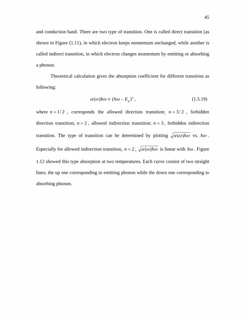
45
and conduction band. There are two type of transition. One is called direct transition (as
shown in Figure (1.11), in which electron keeps momentum unchanged, while another is
called indirect transition, in which electron changes momentum by emitting or absorbing
a phonon.
Theoretical calculation gives the absorption coefficient for different transition as
following:
ngE )()( −∝ ωωωα hh , (1.5.19)
where 2/1=n , corresponds the allowed direction transition; 2/3=n , forbidden
direction transition; 2=n , allowed indirection transition; 3=n , forbidden indirection
transition. The type of transition can be determined by plotting ωωα h)( vs. ωh .
Especially for allowed indirection transition, 2=n , ωωα h)( is linear with ωh . Figure
1.12 showed this type absorption at two temperatures. Each curve consist of two straight
lines; the up one corresponding to emitting phonon while the down one corresponding to
absorbing phonon.
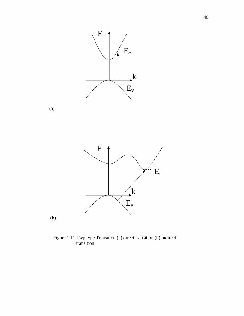
46
Ec
Ev
k
E
Ec
Ev
k
E
Figure 1.11 Twp type Transition (a) direct transition (b) indirect transition
(a)
(b)
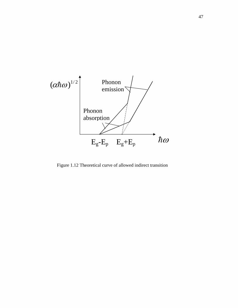
47
ωh Eg+Ep Eg-Ep
Phonon absorption
Phonon emission
2/1)( ωαh
Figure 1.12 Theoretical curve of allowed indirect transition
48
48
Chapter 2
Statement of the Problem
The solid solution of ferroelectrics near morphotropic phase boundary (MPB)
usually exhibits relaxor behavior, with a universal signature of diffuse phase transition
(DPT). Relaxor ferroelectrics has been one of the recent intensified topics in ferroelectric
community both for fundamental understanding and for technical applications [Cross
1987, 1994; Uchino 1994]. Most of the ferroelectric relaxors identified have either the
complex perovskite or the tungsten bronze structure. Except for their anomalously large
and temperature-insensitive dielectric constants, ideal for multilayer capacitors, they also
demonstrate superior characteristics in piezoelectricity, electrostriction and electro-optic
effects applicable to transducer, actuators and optoelectronic devices, practically with
compositions in the vicinity of MPB.
This thesis puts emphases on the optical properties of the single crystal of PBN
and PZN-PT near MPB. The reasons and the main scope are as follows:
First, PBN and PZN-PT are typical relaxors belonging to different families. The
explanation of the mechanism for relaxors is still controversial as introduced in chapter 1
although a lot of progress has been made for their applications. The fact that the
disordering of B-site complex cations played a key role in the phase transition
characteristics for the perovskite structure [Setter 1980] while the A-site vacancy order-
disorder states played a key role in the tungsten bronze structure [Guo 1989] indicates
that the mechanism lies in the nanometer scale or larger. Optical wavelength in the
visible range is an effective probe for nano/micro polar regions. The Burns temperature
Td marks the appearance of significant deviations of refractive index or birefringence
49
49
from a quasilinear temperature dependence [Burns 1983, 1986; Bhalla 1987]. Burns and
Dacol connected this deviation with the onset of the formation of polar nanoregions
(NPR). Dynamic characteristics associated with the sizes of the NPR maybe one of the
significant results expected by measuring of the refractive index and birefringence of
relaxors with different frequency light during phase transition. This study is much needed
to deepen the understanding on relaxors through the investigation of the optical properties
of PBN and PZN-PT.
Second, PBN and PZN-PT are both promising candidates for optonelectronic
devices. Most of the solid state electro-optic oxides have large and fast electro-optic
effects. Single crystals LiNbO3 are the benchmark of electro-optic material used in
telecommunication. However, the high temperature dependence and low electro-optic
effect ( Vpmr /6.1013 = , Vpmr /8.3133 = , Vpmr /6.722 = [Landolt-Bornstein 1996]
prevented it from widespread application. Measurement already demonstrated that the
electro-optic effect of PBN57 ( Vpmr /3213 −= , Vpmr /15433 −= [Guo 2000] and PZN-
12PT ( Vpmr /713 = , Vpmr /13433 = [Lu 2000]) are about 3~5 times of LiNbO3. Some
widely used electro-optic ferroelectrics are listed in Table 2.1. However, a complete
understanding of the optical properties of these materials could not be achieved without
their linear optical properties, including the transmission, refractive index, and
birefringence as well as thermo-optic properties. From these optical properties it is also
interesting to study how the optical bandgap changes with temperature and polarization.
Third, developing a system to accurately, fast, and quantitatively measure
birefringence near phase transition is also our primary objective. The optical properties,
especially indicatrix, of a crystal are related to its symmetry. The birefringence during
50
50
phase transition can be so small that the total phase retardation is less than π and cannot
produce bright and dark fringes for some case, i.e., from tetragonal to cubic and
tetragonal to tetragonal. Thus the conventional fringes pattern measurement method is not
applicable [Zhu 1999,2002].
The thesis is organized according to sequence of the statements above. It includes
7 chapters.
Chapter 1 is the introduction of the background. General properties of
ferroelectrics and relaxor ferroelectrics are introduced first; then some major models for
relaxors are reviewed. Some basic concepts and knowledge that will be used in the latter
chapters are introduced subsequently.
Chapter 3 gives the full account on the experiment results of frequency dispersion
of PBN and PZN-PT near phase transition. Both refractive index and birefringence are
reported. Single oscillator model is used to fit the frequency and temperature dependent
refractive index with only 4 parameters. Optical Curie region is proposed and defined.
Polarization is calculated with frequency and temperature dependent quadratic electro-
optic coefficient.
Chapter 4 addresses the result and discussion about the thermo-optic properties.
Chapter 5 describes the transmission spectrum analysis with emphasis on PZN-PT
for both poled sample and unpoled sample. Optical absorption coefficient and optical
band gap are determined. Urbach rule is used to explain the difference of the absorption
coefficient along the a axis and c axis.
Chapter 6 introduces the theoretical model and experimental configuration on 2D
index mapping.
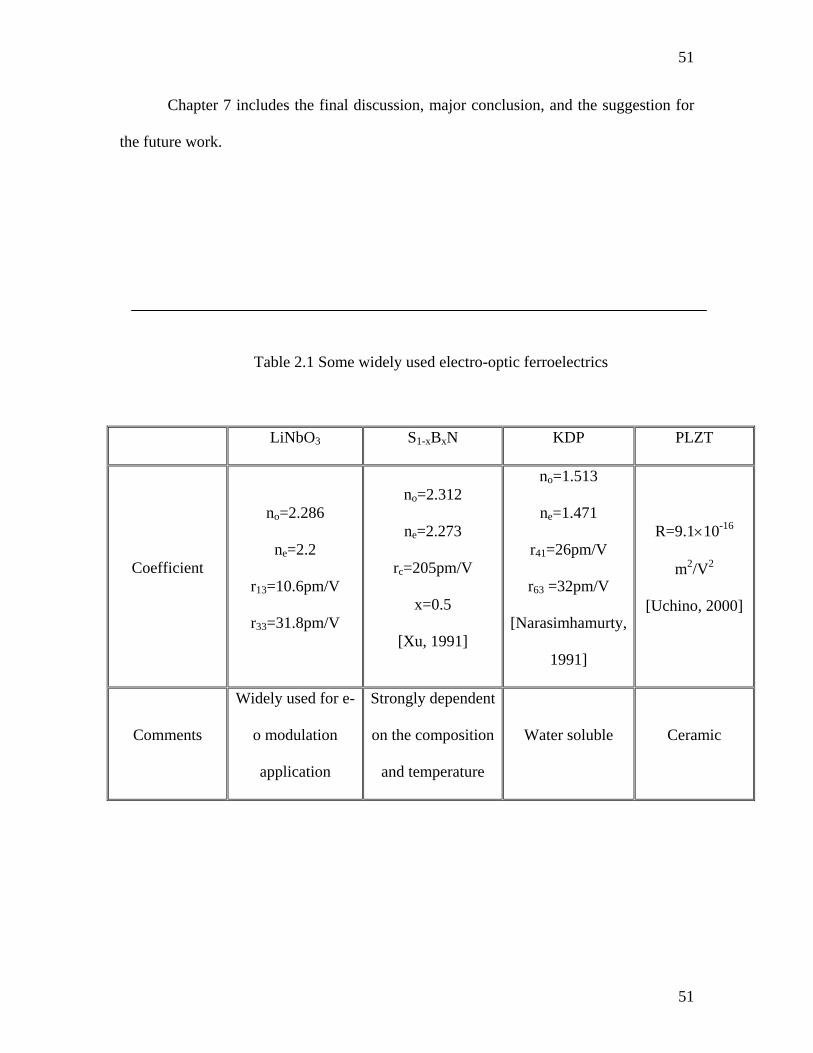
51
51
Chapter 7 includes the final discussion, major conclusion, and the suggestion for
the future work.
Table 2.1 Some widely used electro-optic ferroelectrics
LiNbO3 S1-xBxN KDP PLZT
Coefficient
no=2.286
ne=2.2
r13=10.6pm/V
r33=31.8pm/V
no=2.312
ne=2.273
rc=205pm/V
x=0.5
[Xu, 1991]
no=1.513
ne=1.471
r41=26pm/V
r63 =32pm/V
[Narasimhamurty,
1991]
R=9.1×10⁻¹⁶
m2/V2
[Uchino, 2000]
Comments
Widely used for e-
o modulation
application
Strongly dependent
on the composition
and temperature
Water soluble Ceramic
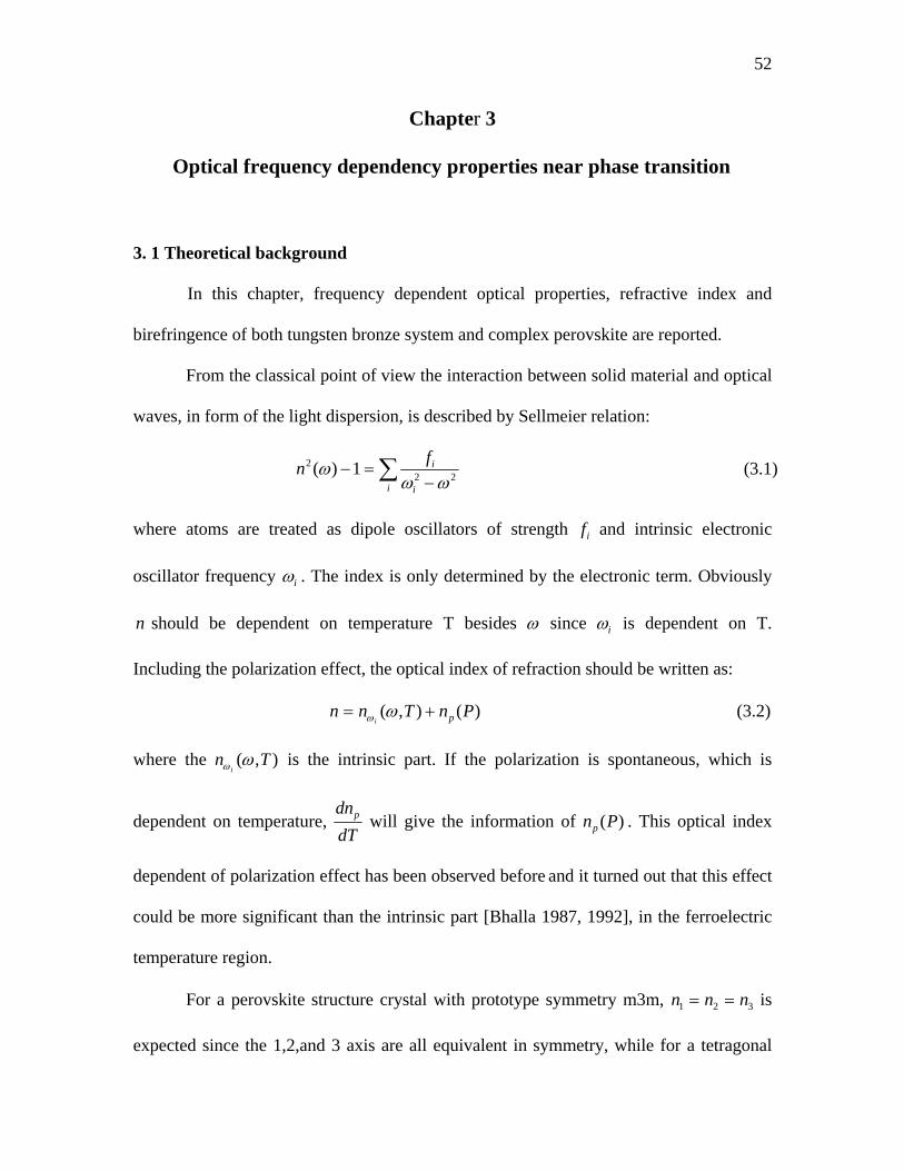
52
Chapter 3
Optical frequency dependency properties near phase transition
3. 1 Theoretical background
In this chapter, frequency dependent optical properties, refractive index and
birefringence of both tungsten bronze system and complex perovskite are reported.
From the classical point of view the interaction between solid material and optical
waves, in form of the light dispersion, is described by Sellmeier relation:
∑ −=−
i i
ifn 222 1)(
ωωω (3.1)
where atoms are treated as dipole oscillators of strength if and intrinsic electronic
oscillator frequency iω . The index is only determined by the electronic term. Obviously
n should be dependent on temperature T besides ω since iω is dependent on T.
Including the polarization effect, the optical index of refraction should be written as:
)(),( PnTnn pi+= ωω (3.2)
where the ),( Tniωω is the intrinsic part. If the polarization is spontaneous, which is
dependent on temperature, dTdnp will give the information of )(Pnp . This optical index
dependent of polarization effect has been observed before and it turned out that this effect
could be more significant than the intrinsic part [Bhalla 1987, 1992], in the ferroelectric
temperature region.
For a perovskite structure crystal with prototype symmetry m3m, 321 nnn == is
expected since the 1,2,and 3 axis are all equivalent in symmetry, while for a tetragonal
53
tungsten bronze crystal with prototype symmetry 4/mmm, 321 nnn ≠= , i.e. there is a
standing birefringence sn13Δ which is dependent upon temperature and optical frequency.
Now if there is a spontaneous polarization Pr along the 3 (c) axis in a cell, this
spontaneous polarization will give an additional long-range dipole-dipole interaction in
this direction except the short-term repulsive forces. So the total birefringence 31nΔ :
)(),( 313131 PnTnn ps Δ+Δ=Δ ω (3.3)
where )(13 Pn pΔ is the birefringence due to the polarization.
Generally the refractive index has appearance of a symmetritrical second-rank
tensor quantity and is represented by the optical indicatrix which is described by equation
1.5.15:
123
2
22
2
21
2
=++nz
ny
nx (3.4)
With the application of an external electric field , the change in index is given by
an expansion expression:
∑∑==
+=−3,2,13,2,1
22 )0(1
)(1
ijkllkijkl
ijkkijk
ijij
EERErnEn
(3.5)
Here )(En and )0(n ( 0n ) are the refractive indices at E and zero field respectively, and
ijkr is the primary electro-optic coefficient (Pockels effect) and ijklR is the quadratic
electro-optic coefficient (Kerr effect).
If using the polarization as the independent variable instead of electric field, the
index change due to the polarization is given by:
∑∑==
− +=Δ3,2,13,2,1
2 )(ijkl
lkijklijk
kijkij PPgPfn (3.6)
54
where ijkf and ijklg are linear polarization-optic coefficient and second polarization-optic
coefficient respectively.
In order to obtain relationship between electro-optic and polarization-optic
coefficient, let the linear term and quadratic term in equation (3.5) and (3.6) equal to each
other, respectively, and using the relation between polarization and electric field,
qpqqpqp EEP )( 00 εεχε −== (3.7)
one can obtain:
)( 0εε −= pqmnqmnp fr (3.8)
))(( 00 εεεε −−= qsprmnrsmnpq gR . (3.9)
For a centro-symmetric prototype symmetry crystal, the linear coefficients ijkf are
zero; equation (3.6) can be written in contracted notation:
∑=Δ − 22 )( siji Pgn (3.7)
For an uniaxial tetragonal prototype ferroelectric crystal with polarization along c-
axis, the induced changed in indices of refraction perpendicular and parallel to the c-axis
are given by:
2313
3011 )(
21 Pgnn −≈Δ (3.8)
2333
3033 )(
21 Pgnn −≈Δ (3.9)
where 03n 0
1n are the index of refraction if there were no polarization of any sort present
along the c axis (n3) and perpendicular to it (n1) respectively. If 001
03 nnn ≈≈ , the change
of optical birefringence due to the polarization will be given by:
55
231333
301331 )(
21)( PggnnnPn p −−=Δ−Δ=Δ (3.10)
Using the model of electric field or spontaneous polarization affecting band gap of
ferroelectrics [Lines and Glass 1977], which gives quadratic electro-optical coefficient
ijg as the formula:
2220
40
0
)(2
ωωσω−
=hn
Bg ij
ij (3.11)
where h
gE=0ω ( gE is band gap) the lowest-energy oscillator frequency, B a constant
related with oscillator strength, ijσ polarization potential.
3.2 Experiment approach
3.2.1 Sample preparation
Single crystal of Pb1-xBaxNb2O6, 1-x=0.57(PBN57) used for this investigation was
grown by Czochralski method. The crystal faces were polished carefully by first using 3
micron diamond paste and then the fine grade 1~1/4 micron diamond paste until an
optical finish (while using kerosene as lubricating medium). Air-dry silver electrodes for
poling the sample and for dielectric constant measurement were also prepared.
The PZN-0.12PT crystals used in this study were grown using the flux method
[Lim and Rajan 2004]. The single crystal was oriental along the <001> direction by using
x-ray Laue back reflection. The same polishing procedure as PBN was also applied to
PZN-PT crystals to an optical grade. The sample was poled at a temperature of 110°C
with an electric field of 10kV/cm for 5 minutes. Then the sample was slowly cooled
down to room temperature under the electric field.
56
3.2.2 Optical refractive index measurement
All optical refractive indices were measured by minimum deviation method with
prism sample. As illustrated in Figure 3.1, the deviation angle Δ of the light beam can be
expressed in terms of the incident angle i of the prism and apex angle A as:
Aniinii −−+=Δ )))/arcsin(sinsin(arcsin()( (3.12)
When the beam within the prism is parallel to the base and passes symmetrically,
the deviation angle has minimum minΔ , and refractive index can be determined as:
)2
sin(
)2
sin( min
A
A
n
Δ+
= (3.13)
The precision of the deviation angle is determined by the minimum vernier scale
of the optical spectrometer of 20′′. So the precision of the measured refractive index can
be approximately as:
4
minminmin
10~)01sin()
2sin(
)2
cos(
)2
sin(
)2
sin()2
20sin(−′′
Δ+
≈
Δ+−
′′+Δ+
= A
A
A
AA
nδ (3.14)
In this study, the optical refractive index measurements were performed from
room temperature up to around 500°C. An Oriel ultraviolet light provided white light.
The white light was selected by a monochromator (Kratos Analytical) and output the
desired monochromatic light at wavelength of 450, 535,633, and 694nm. Then the light
was polarized by a polarizer to ensure that the real extraordinary index ne (n3) was
measured. All the prism apex angle and minimum deviation angles were measured by
Gaertner spectrometer (Figure 3.2) (Scientific Corporation) with a smallest vernier
reading of 20′′. The sample temperature was controlled by a lab-designed hot stage.
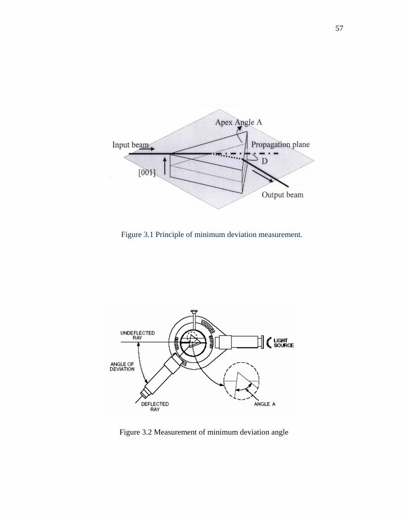
57
Figure 3.1 Principle of minimum deviation measurement.
Figure 3.2 Measurement of minimum deviation angle
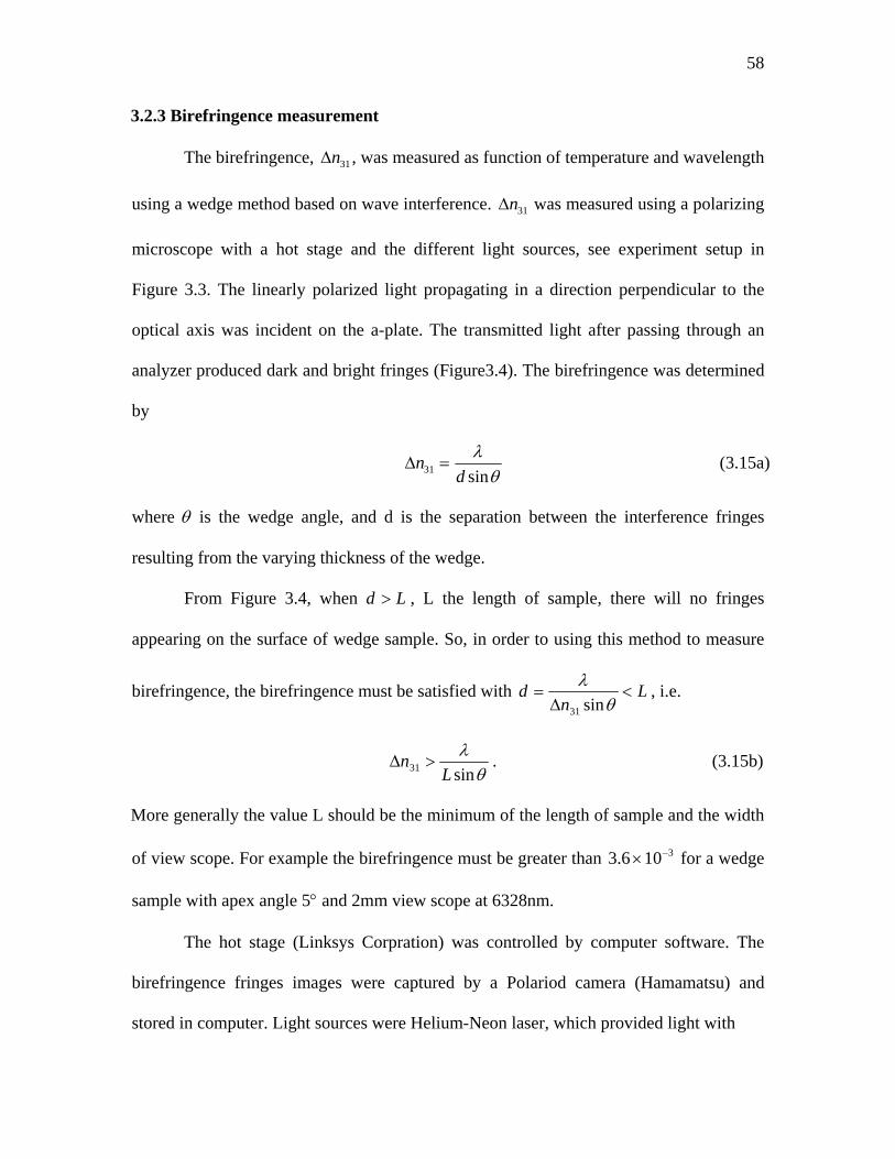
58
3.2.3 Birefringence measurement
The birefringence, 31nΔ , was measured as function of temperature and wavelength
using a wedge method based on wave interference. 31nΔ was measured using a polarizing
microscope with a hot stage and the different light sources, see experiment setup in
Figure 3.3. The linearly polarized light propagating in a direction perpendicular to the
optical axis was incident on the a-plate. The transmitted light after passing through an
analyzer produced dark and bright fringes (Figure3.4). The birefringence was determined
by
θ
λsin31 d
n =Δ (3.15a)
where θ is the wedge angle, and d is the separation between the interference fringes
resulting from the varying thickness of the wedge.
From Figure 3.4, when Ld > , L the length of sample, there will no fringes
appearing on the surface of wedge sample. So, in order to using this method to measure
birefringence, the birefringence must be satisfied with Ln
d <Δ
=θ
λsin31
, i.e.
θ
λsin31 L
n >Δ . (3.15b)
More generally the value L should be the minimum of the length of sample and the width
of view scope. For example the birefringence must be greater than 3106.3 −× for a wedge
sample with apex angle 5° and 2mm view scope at 6328nm.
The hot stage (Linksys Corpration) was controlled by computer software. The
birefringence fringes images were captured by a Polariod camera (Hamamatsu) and
stored in computer. Light sources were Helium-Neon laser, which provided light with
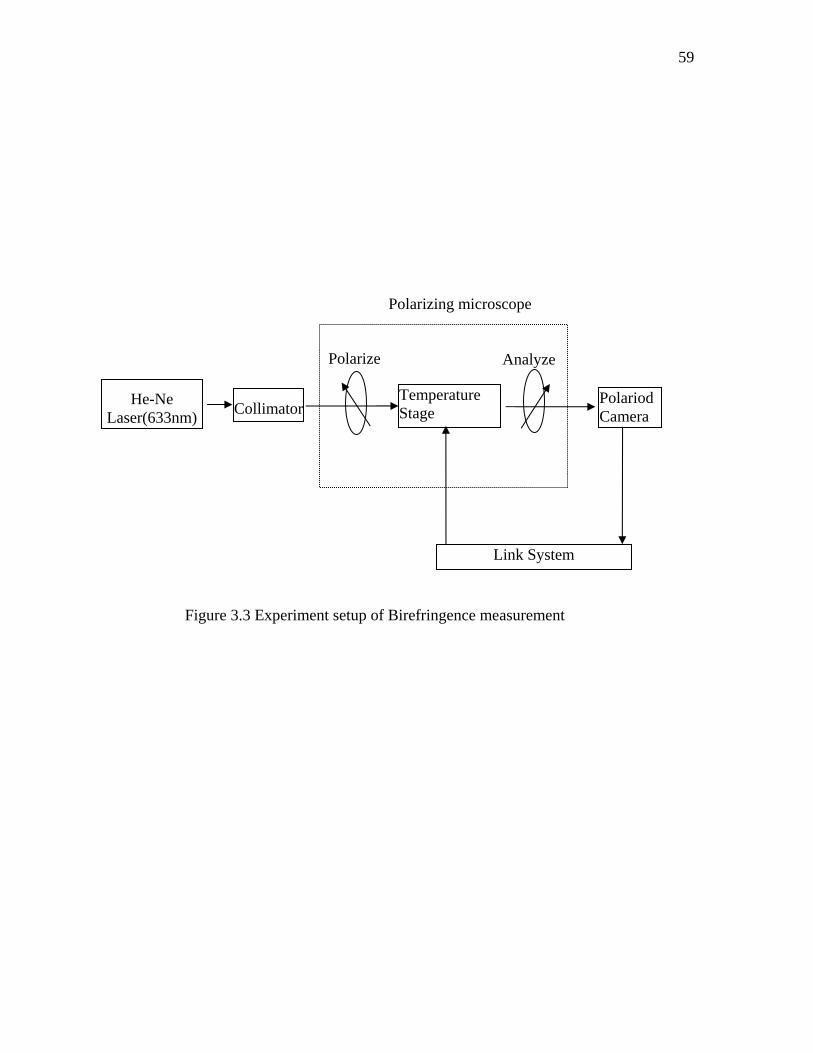
59
He-Ne Laser(633nm) Collimator
Link System
Polariod Camera
Temperature Stage
Polarize Analyze
Polarizing microscope
Figure 3.3 Experiment setup of Birefringence measurement
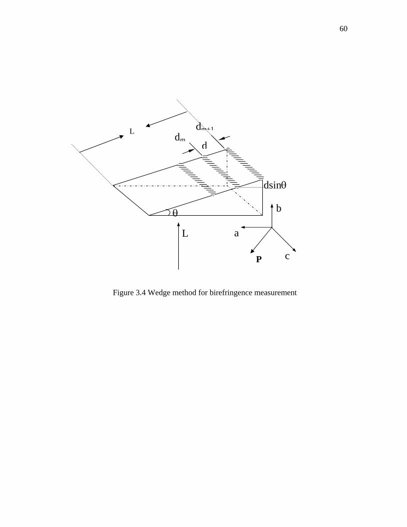
60
P
a
c
d
θ
dsinθ
dm
dm+1
b
L
Figure 3.4 Wedge method for birefringence measurement
L
61
wavelength of 632.8nm, white light with different interference filters, providing light
with wavelength of 535nm and 694nm.
3.3 Optical properties of PBN
3.3.1 PBN system and background Ferroelectric TB is transparent in the visible range and has prototype tetragonal
symmetry 4mm/m. The structure of the TB prototype is shown in Figure 1.6 as projected
in the (001) plane. The tetragonal unit cell consists of 10 BO6 octahedral linked by their
corners in such a manner as to form three different types of tunnels running right through
the structure parallel to the c-axis. A large number of compound crystallize with TB
structure, but the variety, the size and charge of the metal cations can cause subtle
changes on the ferroelectrics phases and varying characteristics of ferroelectric properties.
For example, PbTa2O6 is orthorhombic both above and below Tc, whereas PbNb2O6 is
tetragonal above and orthorhombic below Tc, and Sr1-xBaxNb2O6 (SBN) remains
tetragonal both above and below Tc.[Lines and Glass 1977]
Pb1-xBaxNb2O6 (PBN[(1-x)%]) crystals have a prototype 4/mmm tetragonal
symmetry above their Curie temperature, Tc . Below Tc , PBN has a nearly vertical
morphotropic phase boundary (MPB) near 63.01 =− x which separates the subsolidus
region into two ferroelectric phase fields with two distinct crystallographic structures, as
shown in Figure 3.5. A spontaneous, reversible polarization Pr, is along the c axis (<001>)
for the Ba-rich ( 63.01 ≤− x ) material, which is tetragonal 4mm structure, with only 180°
domains; or perpendicular to the c axis for the Pb-rich ( 63.01 ≥− x ) material, which has
an orthorhombic m2m structure, with 180° and 90° domains [Guo et al 1990]. Like other
TB materials, PBN has a high optical refractive index and the transmission covers
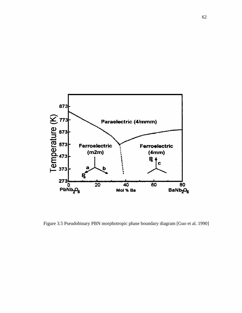
62
Figure 3.5 Pseudobinary PBN morphotropic phase boundary diagram [Guo et al. 1990]
63
roughly from 350nm to 6μm as reported for the SBN. PBN is water-insoluble, chemically
stable and mechanically strong like other ferroelectric oxide octahedral structure crystal.
For the compositions near the MPB, the material possesses temperature insensitive
dielectric constant and polarization, which are advantageous for the electrooptic
applications over a wide temperature range. Around the MPB, this material, either as
single-crystal or in polycrystalline ceramic, shows high-dielectric permittivity,
pyroelectric, piezoelectric, and electro-optic coefficients. All these properties make it
very attractive for applications in electro-optic, surface acoustic wave, pyroelectric, and
memory devices. PBN has been comprehensively studied for the ferroelectric and
electrooptic properties, and the polarization mechanism [Guo et al 1989, 1990a,
1990b;Burns et al 1990; Randall et al 1991;Xiao et al 1996; Yang et al 2003; Santos
2003].
The composition quoted in the thesis as PBN[(1-x)%] where (1-x)% is the mole
percent of PbNb2O6 in the Pb1-xBaxNb2O6, refers to the post-growth analysis composition
as determined by electron microprobe analysis.
One of the characteristics of relaxor ferroelectrics is the very strong frequency
dependence of the electric properties. But most investigations on diffuse phase transition
are limited in the radio frequencies range or lower frequencies. Here the frequency
dependence of the diffuse phase transition of PBN in the optical range is studied.
3.3.2 Experiment results
3.3.2.1 Optical refractive index of PBN
64
The apex angle of the prism sample was determined as 5°7′. The refractive indices
3n of PBN were measured with several visible wavelengths from room temperature to
around 500°C by minimum deviation method as shown in Figure 3.6. The optical index
can be described by a single oscillator model [DiDomenico and Wemple 1969a,b]:
220
020
2
20
202 1
EEEESn d
−=
−=−
λλλλ (3.16)
where 0E is energy of effective dispersion oscillator, dE is dispersion energy. All the
constants can be determined by plotting 1
12 −n
against 2
1λ
to a straight line least square
fits. Some plotting is shown in Figure 3.7 for several temperatures. The derived 0E and
dE against temperature are plotted in Figure 3.8 and Figure 3.9, respectively. The
effective dispersion oscillator energy follows Varshni’s [Varshni 1967] empirical relation
as:
TBATETE+
−=2
00 )0()( (3.17)
where )0(0E , A and B are parameters to be determined. The dispersion energy can also
be fitted by the similar expression:
TDCTETE dd +
−=2
)0()( (3.18)
where )0(dE , C and D are fitting parameters.
From equations 3.16, 3.17, and 3.18, an empirical expression of refractive index
dependence of temperature and wavelength is obtained as:
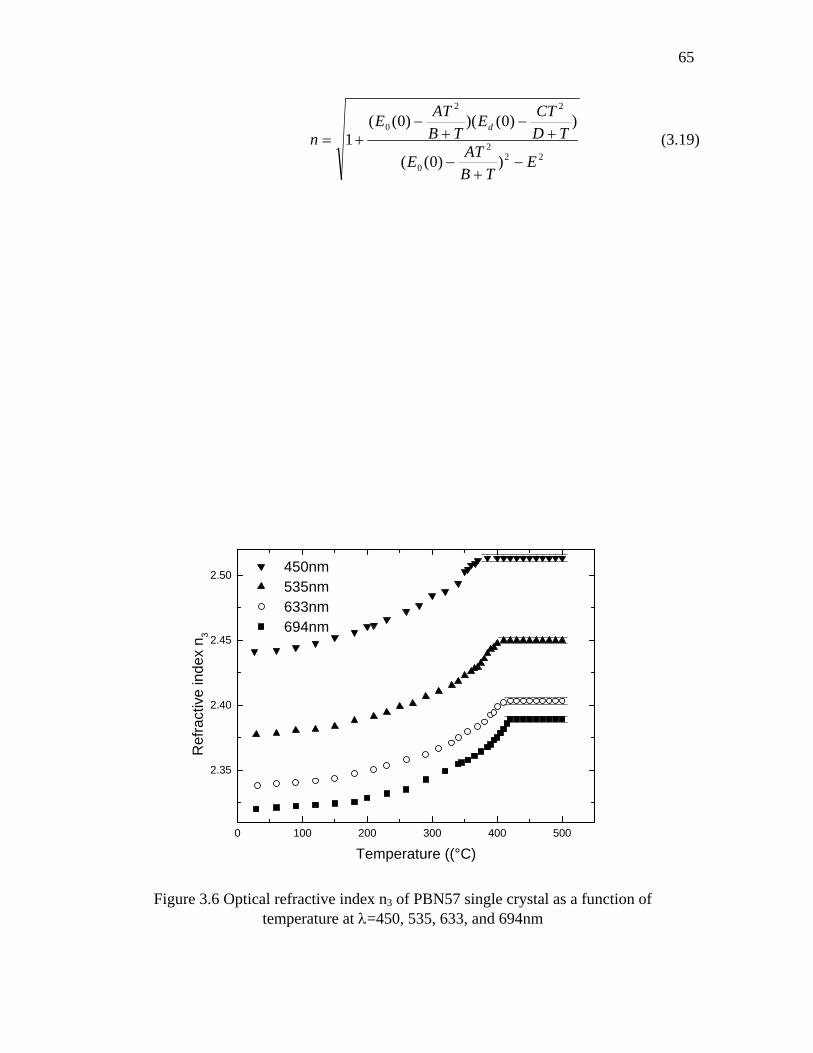
65
222
0
22
0
))0((
))0()()0((1
ETB
ATE
TDCTE
TBATE
nd
−+
−
+−
+−
+= (3.19)
0 100 200 300 400 500
2.35
2.40
2.45
2.50
450nm 535nm 633nm 694nm
Ref
ract
ive
inde
x n 3
Temperature ((°C)
Figure 3.6 Optical refractive index n3 of PBN57 single crystal as a function of
temperature at λ=450, 535, 633, and 694nm
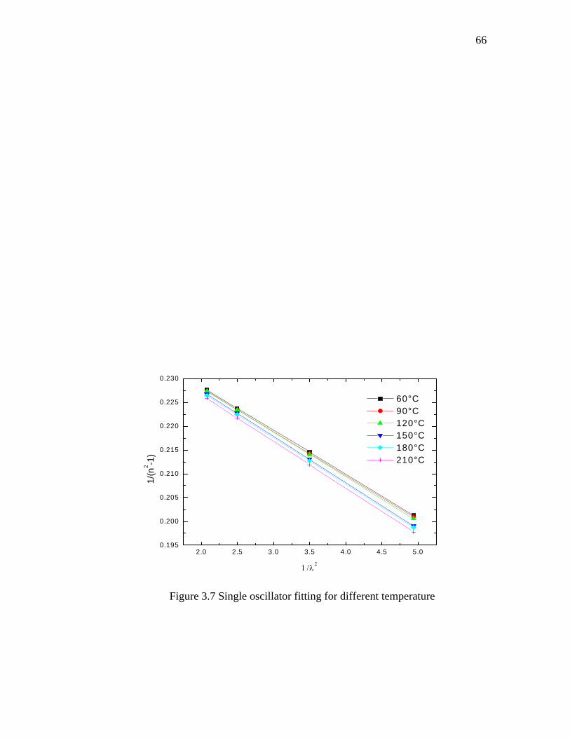
66
2.0 2.5 3.0 3.5 4.0 4.5 5.00.195
0.200
0.205
0.210
0.215
0.220
0.225
0.230
60°C 90°C 120°C 150°C 180°C 210°C
1/(n
2 -1)
1/λ2
Figure 3.7 Single oscillator fitting for different temperature
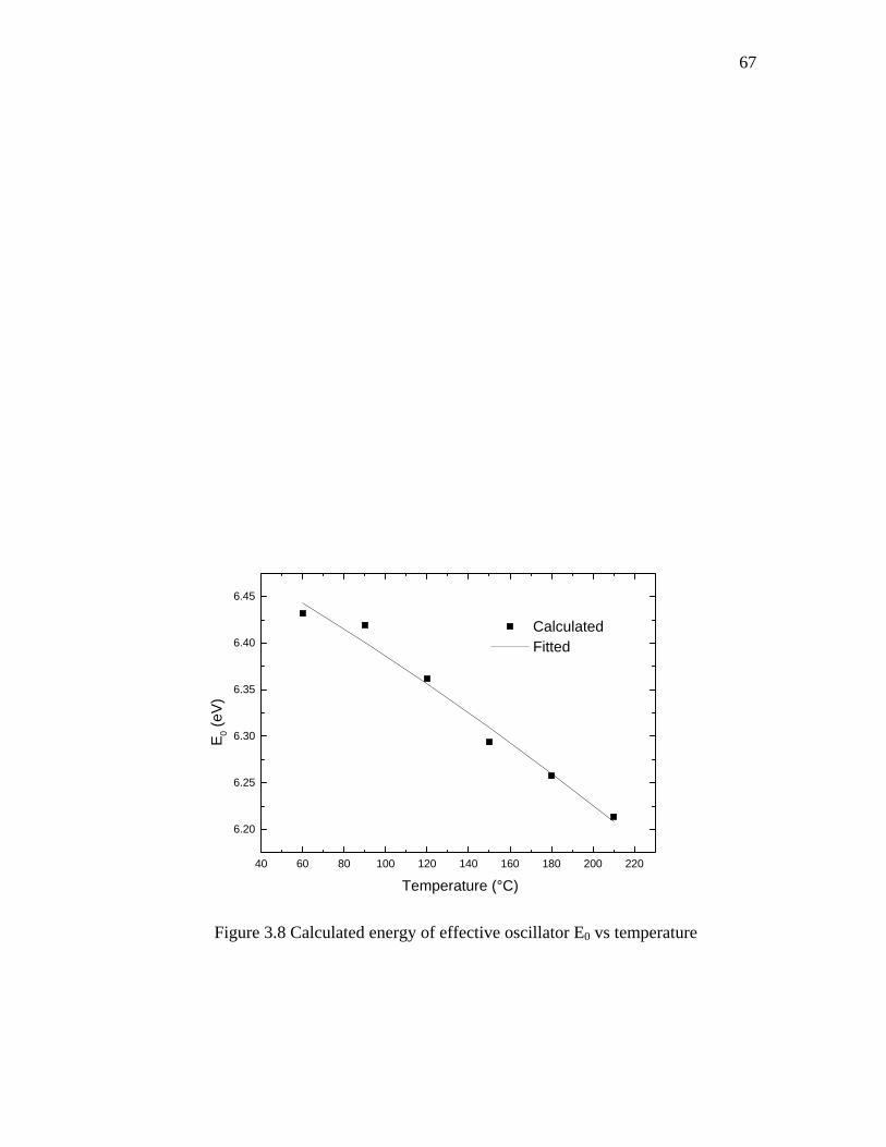
67
40 60 80 100 120 140 160 180 200 220
6.20
6.25
6.30
6.35
6.40
6.45
Calculated Fitted
E 0 (eV
)
Temperature (°C)
Figure 3.8 Calculated energy of effective oscillator E0 vs temperature
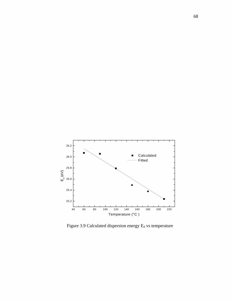
68
40 60 80 100 120 140 160 180 200 220
25.2
25.4
25.6
25.8
26.0
26.2
Calculated Fitted
E d (eV
)
Temperature (°C )
Figure 3.9 Calculated dispersion energy Ed vs temperature
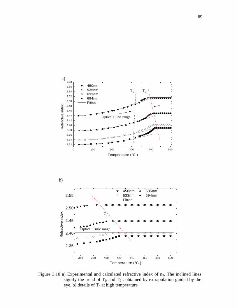
69
0 100 200 300 400 500
2.32
2.34
2.36
2.38
2.40
2.42
2.44
2.46
2.48
2.50
2.52
2.54
2.56
2.58
TdTD
Optical Curie range
450nm 535nm 633nm 694nm Fitted
Ref
ract
ive
inde
x
Temperature (°C )
360 380 400 420 440 460 480 500
2.35
2.40
2.45
2.50
2.55
Td
Optical Curie range
450nm 535nm 633nm 694nm Fitted
Ref
ract
ive
inde
x
Temperature (°C )
Figure 3.10 a) Experimental and calculated refractive index of n3. The inclined lines
signify the trend of TD and Td , obtained by extrapolation guided by the eye. b) details of Td at high temperature
a)
b)
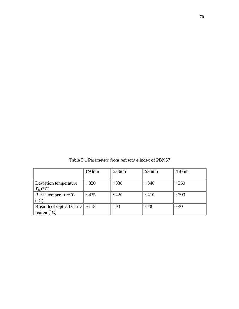
70
Table 3.1 Parameters from refractive index of PBN57 694nm 633nm 535nm 450nm
Deviation temperature TD (°C)
~320 ~330 ~340 ~350
Burns temperature Td (°C)
~435 ~420 ~410 ~390
Breadth of Optical Curie region (°C)
~115 ~90 ~70 ~40
71
This six-parameter refractive index empirical formula is temperature and
frequency dependent, which is based on the single oscillator model with very clear
physical emphasis. Once the index in the low temperature range, usually convenient to
measure accurately, is known, the index in the whole temperature range which can be
described by single oscillator model can be calculated.
There have been a lot of empirical formulas of refractive index [Schlarb and
Betzer 1993; Abedin and Ito 1996], but almost they have no physical meaning.
Using the parameters in expressions 3.18 and 3.19, the refractive index against
temperature is plotted in Figure 3.10. From room temperature to 340°C for 450nm and to
320°C for 694nm, the fitting values showed excellent agreement with experimental data.
However, the index fitted deviates from the experiment data at different temperatures,
denoted as TD, well below Tm for each wavelength in ferroelectric state.
This deviation temperature from the single oscillator model, TD, marks perhaps
the breaking up of the macroscopic polar regions approaching a relaxor phase transition.
TD shifts to higher temperature for probing light of higher frequency (a similar trend is
found for isotropic temperature Ti, see next section). During the phase transition process
for relaxor ferroelectric, the polarization not only presents on the ionic scale as the usual
elementary dipole moments of atoms, but also exists in the micro/nanoscale due to the
polar regions. [Randall and Bhalla 1990a; Randall et al.1990b]. Taking into account the
dipole-dipole cluster interaction between polar regions in equation 3.2, the index should
72
be larger than that contained in the electronic terms alone. This explains the deviation
that the fitted index values are smaller than the measurement values above the deviation
temperature TD.
There is an error for refractive index at the high temperature (>400°C) range.
When measuring the sample in this high temperature range, the refractive ray is not as
stable as in the low temperature. However, there is no obvious change of the angle of the
refractive ray in the whole high temperature range. The error is around 0.002. So the
refractive index may not keep the same but has a slight slope of in the range of
000025.0± . This error may come from the temperature fluctuation resulted from the
heating couple or the structure of sample itself.
It is well known that at high temperature in paraelectric state the refractive index
n3 scales linearly with temperature and can be fitted by a linear relation with temperature.
Below a certain phase transition or characteristic temperature refractive index will not
follow this linear behavior. This departure-temperature is often regarded as dipole
temperature or Burns temperature, Td. [Burns and et. al. 1986,1987,1990a, b]. The Burns
temperatures for different frequency are listed in table 3.1. Burns temperature marks the
appearance of the local nonreversible polarization.
As mentioned above, there is an error around 0.0002 for refractive index in the
high temperature range and may result a very large error of the Burns temperature. Here
the start point of the unstable refractive index is regarded as Burns temperature, however,
this is possibly not the truly Burns temperature. In later section 3.3.2.4 the dielectric
maxima is found around 365°C for heating run. The difference between the Burns
temperature derived from optical refractive index n3 and dielectric maxima is just ~25°C
73
for 450nm and ~70°C for 694nm, which are much smaller than those reported in previous
papers, which are usually about up to 200°C for typical relaxor ferroelectrics [Burns et. al.
1986, 1987, 1990a, b, Bhalla et. al. 1987, 1992]. One the other hand, the profile of
refractive index of PBN57 is more like a 2nd order phase transition, similar as PBN50
[Burns et. al. 1990c], which is far from the MPB and is normal ferroelectrics, but rather a
typical realxor transition, although PBN57 is very close to the MPB. It implies the diffuse
index α is more close to 1 but rather 2. This is also supported by the later dielectric
constant measurement in section 3.3.2.4 where the dielectric constant is weak dependent
on frequency The difference between Burns temperature and temperature of dielectric
maxima is zero for normal ferroelectric with diffuseness coefficient of 1 and several
hundred degrees for "complete" relaxor ferroelectrics with diffuseness coefficient of 2.
It's reasonable to assume that the difference between Burns temperature and temperature
of dielectric maxima is proportional to diffuseness coefficient α . The validity of this
assumption is based on the two facts. First, the diffuseness coefficient is increasing with
the degree of disorder of polar regions [Setter and Cross, 1980]. Second, the Burns
temperature is approximately the same as the Tc of the end member, AB'O3 of the mixed
system A(B'B")O3 [Burns, 1985]. With the above assumption the small difference
between Burns temperature and temperature of dielectric maxima of PBN57 is accepted.
Optical Curie region is proposed to define as the temperature between the
deviation temperature TD and the Burns temperature Td. The optical Cuie region is about
40°C for 450nm and 115°C for 694nm. All these parameters are listed in table 3.1 and
plotted in Figure 3.14. It is evident that the optical Curie region broadens at lower
frequency, which agrees in trend with Curie region for dielectric constant [Cross, 1987]
74
and that of the result of birefringence. Moreover, the width of the optical Curie region
scales almost linearly with frequency.
In ferroelectric state, the wavelength of high frequency light (blue light) is closer
the size of nanocluster than the wavelength of low frequency light (red light). Thus it’s
more effective for blue light to active the nanocluster.
3.3.2.2 Birefringence of PBN
Birefringence results of PBN obtained at wavelength of 694nm, 633nm, and
535nm are shown in Figure 3.11. All three birefringence undergo positive, zero
(isotropic), and negative from high temperature to low temperature while refractive index
of the PBN crystal changed from optically positive to optically negative. The higher the
frequency of the light, the larger the birefringence. This is expected considering the
general dispersion theory based on the model of the classical harmonic oscillator
interacting with external field while the intrinsic frequency in equation (3.1) is taken as
the lowest-energy oscillator frequency 0ω . For a typical ferroelectrics band gap gE ~4-
5eV, 0ω (>1015 Hz) is always much greater than source light frequencyω (visible light
frequency 1014 Hz). In the normal dispersion region when the light frequency is
approaching to its intrinsic frequency of the oscillator, the electronic polarizability is high
along the c-axis thus the large refractive index along the c-axis; while the refractive index
along the a-axis remains approximately constant, thus positive birefringence is resulted.
A more detailed birefringence-temperature relation is shown in Figure 3.12. The
optical isotropic temperature Ti increases with frequency of light. Ti in ferroelectric
tungsten bronze strontium barium niobates was reported before [Bhalla, 1987, 1992,
Ivanov, 2002]; however, its physical significance in relaxor materials has not been
75
discussed previously. Below Ti the primary contribution to 31nΔ comes from spontaneous
polarization whose characteristic resonance frequency is 2~3 orders lower than that of
electronic polarization. Negative 31nΔ is thus observed in analogous to the anisotropy of
dielectric permittivity 31 εε > . Similarly Tm, the temperature corresponding to maximum
dielectric constant at low frequency, and TD, deviating temperature from single oscillator
model (to be addressed in a later section), have the same tendency increasing with
frequency.
It is well known that at high temperature in paraelectric state the birefringence is
the standing birefringence that scales linearly with temperature and can be fitted by a
linear relation with temperature. Below a certain phase transition or characteristic
temperature birefringence will not follow this linear behavior. This departure-
temperature is regarded as dipole temperature or Burn’s temperature, Td. [Burns, 1985].
This departure is nearly 100°C above the isotropic temperature Ti for the sample studied.
The derived Td and measured Ti are listed in table 3.2. Td is also frequency dependent but
in contrast to that of Ti it decreases with frequency. (Td-Ti) is listed in Table 3.2 that
decreases at higher frequency. The slopes of the fitted straight lines in Figure 3.12 also
increase with frequency. It implies that light with higher frequency has higher resolution
to smaller polar-regions as well. All these values are tabulated in Table 3.2.
From equation 3.3, the combination of the standing birefringence 031nΔ and the
polarization-dependent part vanishes that leads to the optical isotropic condition.
Standing birefringence is dominated by anisotropic ionic polarizability whose
temperature dependence comes from lattice deformation. The standing birefringence is
linear with temperature with a positive slope while the polarization-dependent part is of
76
negative dependence in ferroelectric state and gradually decreases approaching dipole
temperature Td. Before reaching to the dipole temperature Td, the standing birefringence
and polarization-dependent part compensate each other at isotropic temperature Ti. In
relaxor ferroelectrics the macrodomain transforms to microdomain with increasing
temperature [Yao et.al. 1984], and so do the polar regions. Considering coupling
between light waves and polar regions, apparently a certain frequency will be more
sensitive to some polar regions with a corresponding sizes but almost invisible to other
polar regions with much different sizes. When temperature is increased, the size of polar
region becomes smaller and is sensitive to light of shorter wavelength. Thus light of low
frequency is more effective to probe the polar region at low temperature comparing with
light of high frequency. So the frequency of the light that can sense effectively polar-
regions is increasing with temperature. The statistical result of this effective interaction
is that 31nΔ approaches to zero at a lower temperature for lower frequency since the
number of polar-regions of corresponding sizes decreasing at lower temperature, i.e., the
isotropic temperature, Ti, increases with frequency.
From equation (3.10), the root mean square −
23P can be obtained from )( 31nΔδ
which is the difference between the measurement 31nΔ and the standing birefringence
sn31Δ extrapolated from high temperature linear region. Here 32.2031 =≈≈ nnn [ Isupov,
1989], and 0755.01333 =− gg (m4/C2) [Guo et al. 1990] at nm633=λ . In order to get the
quadratic electro-optical coefficient for other two frequencies, the equation (3.11) is used.
Since 0ω (>1015 Hz) is always much greater then ω (visible light frequency 1014 Hz) and
not dominate on g value, the choosing of 0ω will not change g too much. Using these
parameters, the g values are calculated and listed in table 3.2.
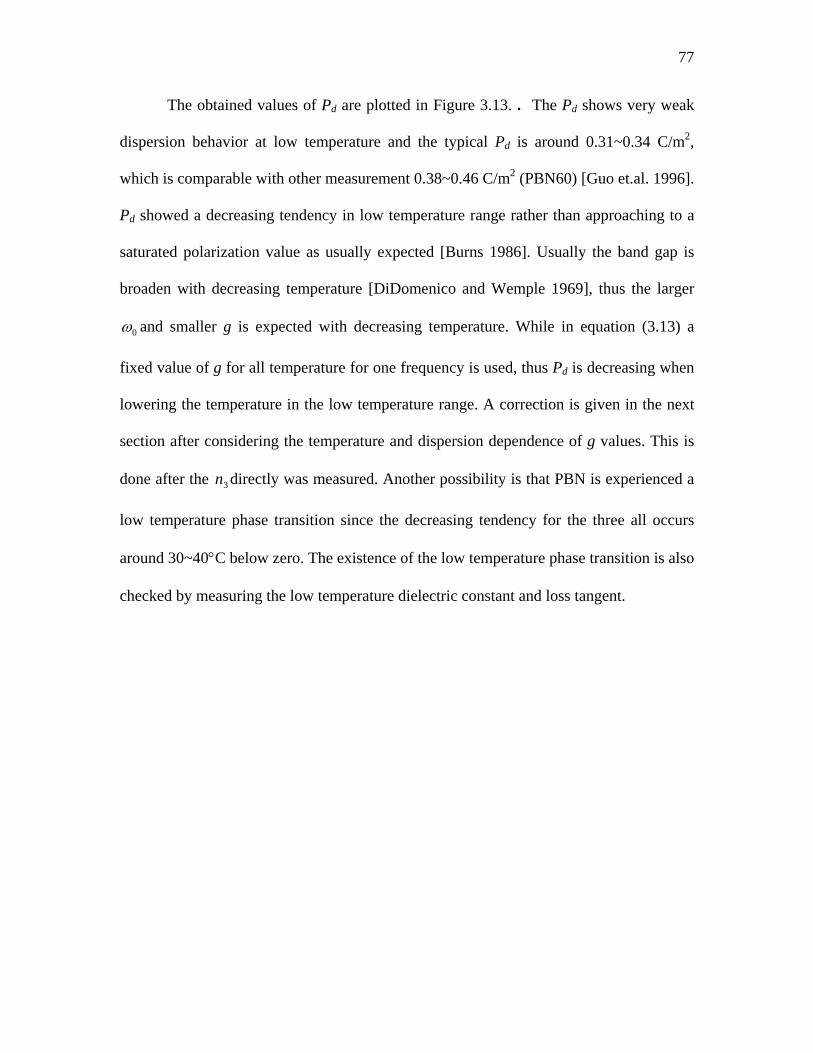
77
The obtained values of Pd are plotted in Figure 3.13. . The Pd shows very weak
dispersion behavior at low temperature and the typical Pd is around 0.31~0.34 C/m2,
which is comparable with other measurement 0.38~0.46 C/m2 (PBN60) [Guo et.al. 1996].
Pd showed a decreasing tendency in low temperature range rather than approaching to a
saturated polarization value as usually expected [Burns 1986]. Usually the band gap is
broaden with decreasing temperature [DiDomenico and Wemple 1969], thus the larger
0ω and smaller g is expected with decreasing temperature. While in equation (3.13) a
fixed value of g for all temperature for one frequency is used, thus Pd is decreasing when
lowering the temperature in the low temperature range. A correction is given in the next
section after considering the temperature and dispersion dependence of g values. This is
done after the 3n directly was measured. Another possibility is that PBN is experienced a
low temperature phase transition since the decreasing tendency for the three all occurs
around 30~40°C below zero. The existence of the low temperature phase transition is also
checked by measuring the low temperature dielectric constant and loss tangent.
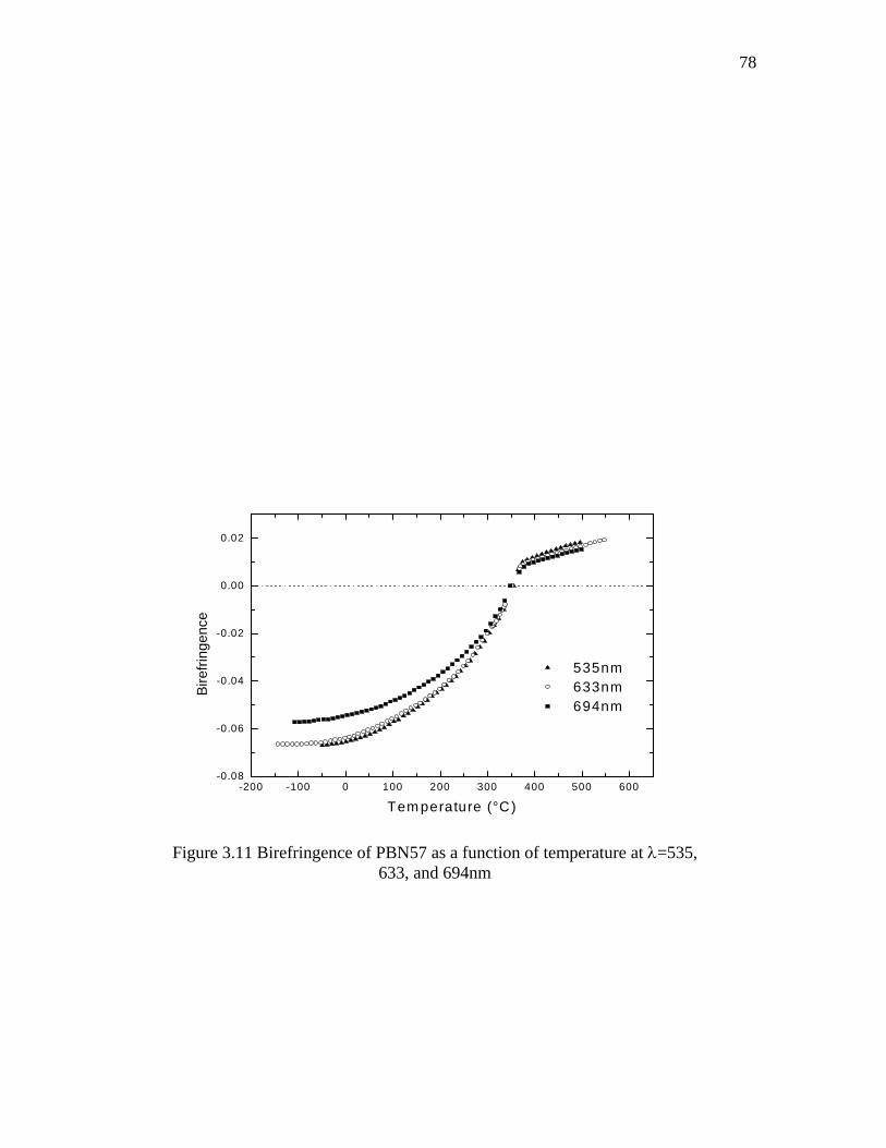
78
-200 -100 0 100 200 300 400 500 600-0.08
-0.06
-0.04
-0.02
0.00
0.02
535nm 633nm 694nm
Bire
fring
ence
Tem perature (°C)
Figure 3.11 Birefringence of PBN57 as a function of temperature at λ=535,
633, and 694nm
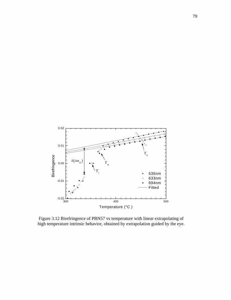
79
300 400 500-0.02
-0.01
0.00
0.01
0.02
Td
Tm
Ti
δ(Δn31)
535nm 633nm 694nm Fitted
Bire
fring
ence
Temperature (°C )
Figure 3.12 Birefringence of PBN57 vs temperature with linear extrapolating of high temperature intrinsic behavior, obtained by extrapolation guided by the eye.
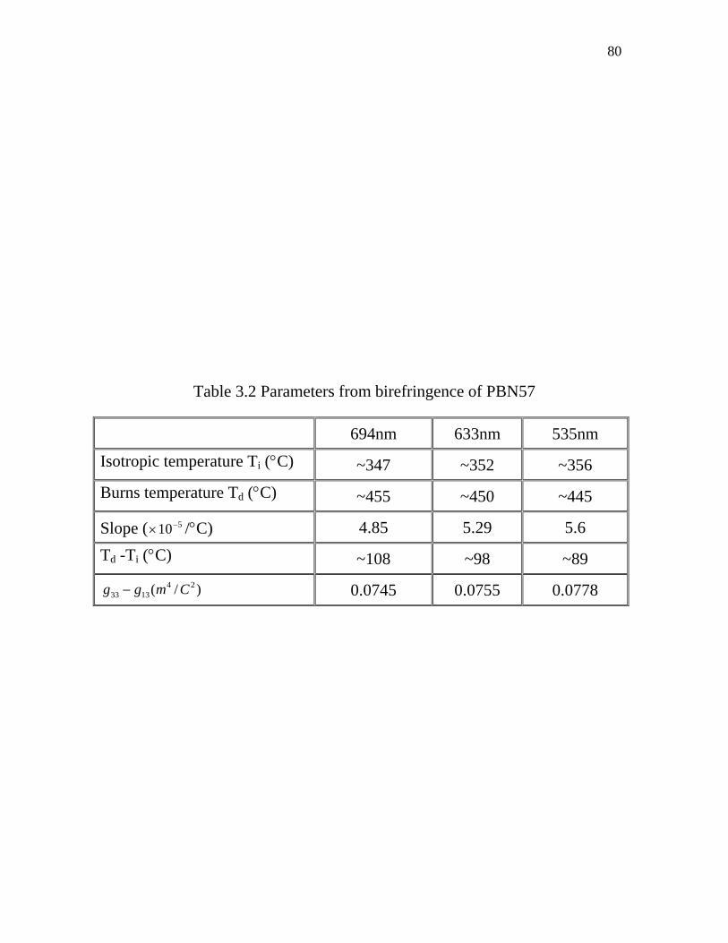
80
Table 3.2 Parameters from birefringence of PBN57
694nm 633nm 535nm Isotropic temperature Ti (°C) ~347 ~352 ~356
Burns temperature Td (°C) ~455 ~450 ~445
Slope ( 510−× /°C) 4.85 5.29 5.6
Td -Ti (°C) ~108 ~98 ~89
)/( 241333 Cmgg − 0.0745 0.0755 0.0778
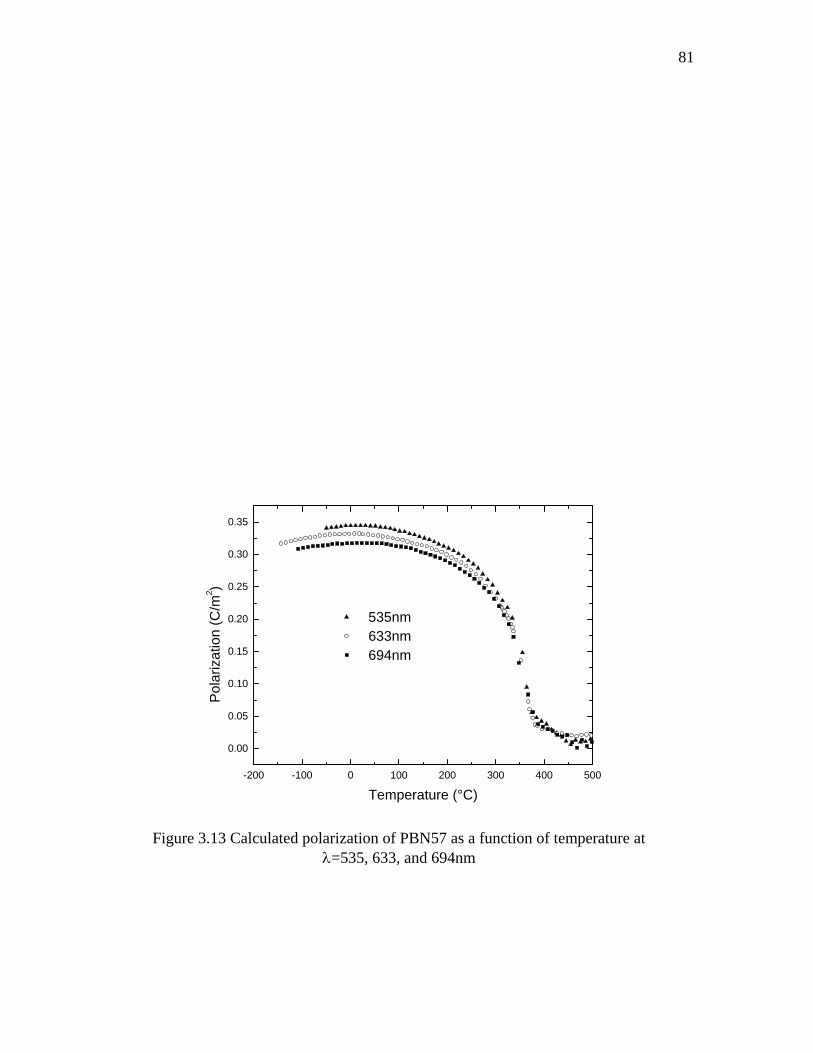
81
-200 -100 0 100 200 300 400 500
0.00
0.05
0.10
0.15
0.20
0.25
0.30
0.35
535nm 633nm 694nm
Pol
ariz
atio
n (C
/m2 )
Temperature (°C)
Figure 3.13 Calculated polarization of PBN57 as a function of temperature at
λ=535, 633, and 694nm
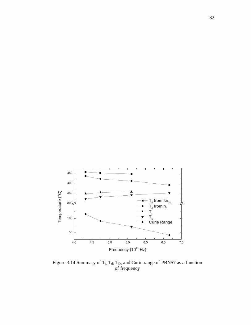
82
4.0 4.5 5.0 5.5 6.0 6.5 7.0
50
100
300
350
400
450
Td from Δn31
Td from n3
Ti TD Curie RangeTe
mpe
ratu
re (°
C)
Frequency (1014 Hz)
Figure 3.14 Summary of Ti, Td, TD, and Curie range of PBN57 as a function
of frequency
83
3.3.2.3 Correction of Polarization:
Presently there are no available reference for the frequency and temperature
dependent values of quadratic electro-optical coefficients of PBN. From equation (3.11)
and (3.19), the quadratic electro-optical coefficient 33g has been calculated from around -
150 °C to 350 °C and plotted in Figure 3.15, which shows a considerable dependence
upon temperature but small dependence on frequency. The data of dispersion of electro-
optic effect for ferroelectric is sparse to the author. Arabidze and Chikvaidze [Arabidze
and Chikvaidze, 1979] measured the temperature dependence quadratic electro-optic
coefficient of barium titanate at three wavelengths 460nm, 500nm, and 600nm. Their
results showed that the quadratic electro-optic coefficient was very dependent on the
temperature and frequency.
The phase transition has not been considered in this calculation since 33g maybe
experience an abruptly change during the phase transition. So the calculated values of
33g near and above Tm is not reliable. However, this would not effect results the
calculation of polarization. In equation (3.10) )( 31nΔδ is near zero above Tm, ensuring the
values of Pd near zero no matter the values of 33g .
The polarization estimated using corrected electro-optical coefficients is plotted in
Figure 3.16. The decreasing tendency of polarization obtained without correction for 535
nm and 694nm is no longer present. In the low temperature range for the 633nm, a
84
slightly decreasing tendency still exists but occurs at a lower temperature around -100 °C,
shifting about 60°C to lower temperature. The above correction is qualitative, a
quantitative correction maybe available after more rigorous model for optical refractive
index and g value.
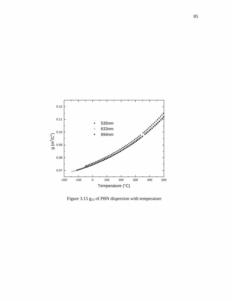
85
-200 -100 0 100 200 300 400 500
0.07
0.08
0.09
0.10
0.11
0.12
535nm 633nm 694nm
g (m
4 /C2 )
Temperature (°C)
Figure 3.15 g33 of PBN dispersion with temperature
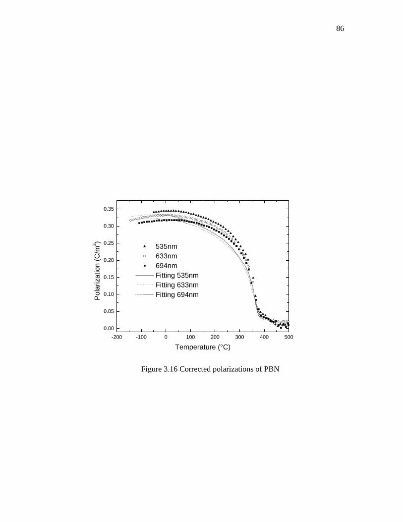
86
-200 -100 0 100 200 300 400 5000.00
0.05
0.10
0.15
0.20
0.25
0.30
0.35
535nm 633nm 694nm Fitting 535nm Fitting 633nm Fitting 694nm
Pol
ariz
atio
n (C
/m2 )
Temperature (°C)
Figure 3.16 Corrected polarizations of PBN
87
3.3.2.4 Dielectric constant measurement
In order to evaluate fully the results of optical measurement the dielectric
capacitance and loss tangent of the PBN57 crystal was measured using HP4284 LCR
meter from 1KHz to 1M Hz in the temperature range of -260-20°C at rate of 1°C /min
and in the temperature range of 30-460°C at rate of 4°C /min. In figure 3.17 both in the
heating and cooling runs, it's evident that the dielectric constant is not strongly frequency
dependent. For PBN57 having high temperature phase transition (Tc>360°C), there is a
small thermal hysteresis (at ~365°C in the heating and at ~355°C in the cooling run)
However, the isotropic temperature derived from birefringence is lower than the Tm. This
is a signature of the relaxor behavior in PBN solid solution. The low temperature
dielectric constant with temperature is shown in Figure 3.18. There is no evident phase
transition occurring. This supports the previous polarization correction with the
consideration of the temperature and frequency dependent 33g .
Martirena [Martirena and Burfoot, 1974] and Uchino [Uchino and Nomura, 1982]
suggested the variable power law, which is rewritten as:
CTT m
m
α
εε)(11 −
+= (3.20)
where ε and mε are the permittivity and its maximum, respectively, Tm is the
temperature of mε and C and α are fitting parameters. It describes the paraelectric side
88
dielectric permittivity of ferroelectrics with diffuse phase transition. Power factor α close
to 1 suggests normal ferroelectrics, while close to 2 suggests "complete" relaxor
ferroelectrics. The fitting parameters are listed in table 3.3. The power factor of 1.43
suggests PBN57 is not a complete relaxor ferroelectrics.
The freezing temperature Tf can be derived from the Vogel and Fulcher relation
[Viehland et. al. 1990b]:
])(
exp[0fm
a
TTkEff−
−= (3.21)
where Tf is the static freezing temperature, Ea the activation energy, f0 the Debye
frequency, k is Boltzmann's constant. The data listed in table 3.3 is not enough to yield a
reasonable freezing temperature since there are only 4 sets data, however, 3 parameters
need to be determined.
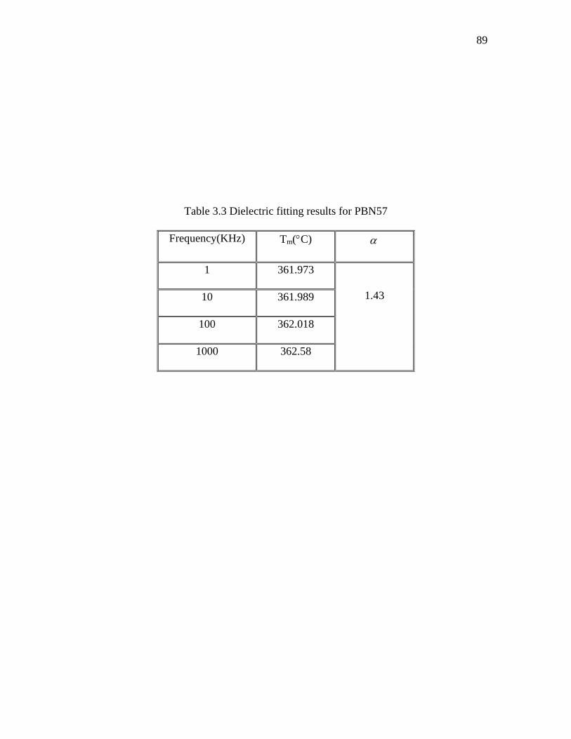
89
Table 3.3 Dielectric fitting results for PBN57
Frequency(KHz) Tm(°C) α
1 361.973
10 361.989
100 362.018
1000 362.58
1.43
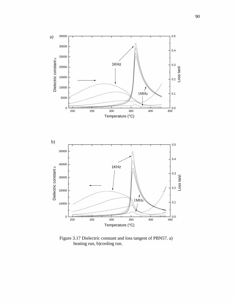
90
200 250 300 350 400 4500
5000
10000
15000
20000
25000
30000
35000
1KHz
Die
lect
ric c
onst
ant ε
Temperature (°C)
0.0
0.1
0.2
0.3
0.4
0.5
Los
s ta
nδ
1MHz
200 250 300 350 400 4500
10000
20000
30000
40000
50000
1KHz
Die
lect
ric c
onst
ant ε
Temperature (°C)
0.0
0.1
0.2
0.3
0.4
0.5
Los
s ta
nδ
1MHz
a)
b)
Figure 3.17 Dielectric constant and loss tangent of PBN57. a) heating run, b)cooling run.
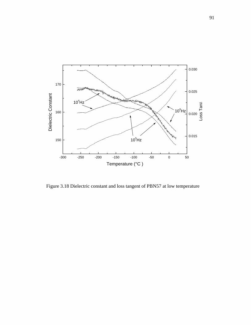
91
-300 -250 -200 -150 -100 -50 0 50
150
160
170
104Hz
105Hz
106Hz
D
iele
ctric
Con
stan
t
Temperature (°C )
0.015
0.020
0.025
0.030
Los
s Ta
nδ
Figure 3.18 Dielectric constant and loss tangent of PBN57 at low temperature
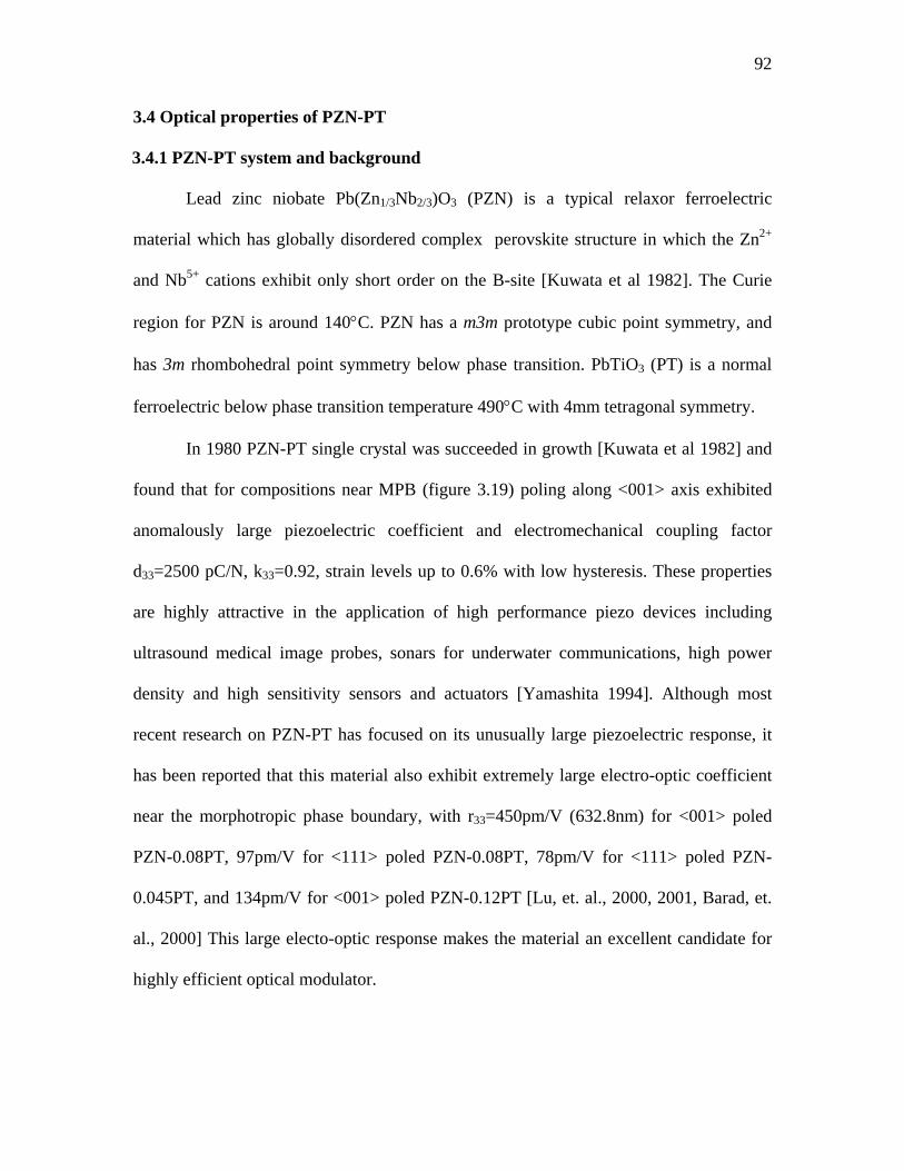
92
3.4 Optical properties of PZN-PT
3.4.1 PZN-PT system and background
Lead zinc niobate Pb(Zn1/3Nb2/3)O3 (PZN) is a typical relaxor ferroelectric
material which has globally disordered complex perovskite structure in which the Zn2+
and Nb5+ cations exhibit only short order on the B-site [Kuwata et al 1982]. The Curie
region for PZN is around 140°C. PZN has a m3m prototype cubic point symmetry, and
has 3m rhombohedral point symmetry below phase transition. PbTiO3 (PT) is a normal
ferroelectric below phase transition temperature 490°C with 4mm tetragonal symmetry.
In 1980 PZN-PT single crystal was succeeded in growth [Kuwata et al 1982] and
found that for compositions near MPB (figure 3.19) poling along <001> axis exhibited
anomalously large piezoelectric coefficient and electromechanical coupling factor
d33=2500 pC/N, k33=0.92, strain levels up to 0.6% with low hysteresis. These properties
are highly attractive in the application of high performance piezo devices including
ultrasound medical image probes, sonars for underwater communications, high power
density and high sensitivity sensors and actuators [Yamashita 1994]. Although most
recent research on PZN-PT has focused on its unusually large piezoelectric response, it
has been reported that this material also exhibit extremely large electro-optic coefficient
near the morphotropic phase boundary, with r33=450pm/V (632.8nm) for <001> poled
PZN-0.08PT, 97pm/V for <111> poled PZN-0.08PT, 78pm/V for <111> poled PZN-
0.045PT, and 134pm/V for <001> poled PZN-0.12PT [Lu, et. al., 2000, 2001, Barad, et.
al., 2000] This large electo-optic response makes the material an excellent candidate for
highly efficient optical modulator.
93
As shown in phase diagram (Figure 3.19), the MPB of (1-x)Pb(Zn1/3Nb2/3)O3-
xPbTiO3 was initially believed to be an almost vertical boundary that separates the
rhombohedral 3m from the tetragonal 4mm phase and located close to the value of x~10%
for PZN-xPT. In addition to the known rhombohedral and tetragonal phases, a recent
advance has been accomplished with the discovery of a new monoclinic phase in PZT
[Noheda et al 1999]. New orthorhombic and monoclinic phases have also been found in
PZN-PT [Noheda et al 2001]. These new phases play a key role in explaining the high
piezoelectric and electrostrictive responses near the MPB. In PZN-PT, the new phase has
an point symmetry mm2 and extends in a narrow concentration range around the MPB
(8%<x<11%) with almost vertical phase boundaries on either side. This new phase can
be described as a ''matching'' phase between the rhombohedral and tetragonal phases.
This means that the polarization vector, instead of being aligned with a particular crystal
axis, may be pointing in an arbitrary direction within a plane, allowing for a very easy
reorientation of the polarization vector. Recently, a model [Fu and Cohen 2000] has been
proposed that connects the structural features of the lead relaxor systems with their
unusual polarization properties.
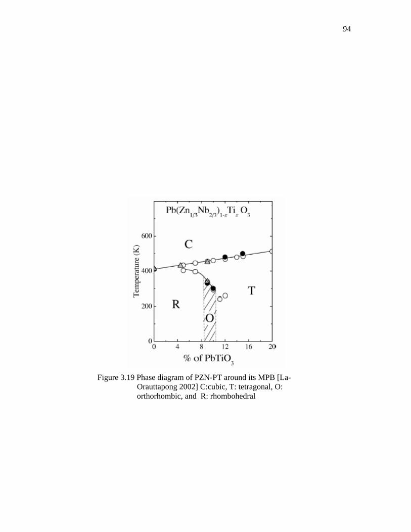
94
Figure 3.19 Phase diagram of PZN-PT around its MPB [La-Orauttapong 2002] C:cubic, T: tetragonal, O: orthorhombic, and R: rhombohedral
95
3.4.2 Experiment results of optical refractive index
The apex angle of prism sample was determined as 7°22′. The optical refractive
indices 3n of PZN-0.12PT single crystal were measured by minimum deviation method
both before and after poling with wavelengths 450nm, 535nm, 633nm, and 694nm from
room temperature to around 350°C as shown in Figure 3.20 and Figure 3.21. Both of the
index data sets exhibit normal dispersion behavior. After poling the refractive indices 3n
decrease drastically by 0.17 for 694nm and 0.1 for 450nm. This is consistent with the
dielectric constant measurement that after poling the dielectric constant decreases
significantly from 4000 to 700[Zhang, unpublished data]. Lu [Lu 2000] measured
refractive index of the PZN-0.12PT with n3=2.46±0.01 and n1=2.57±0.01 by Brewster's
angle at 633nm. The refractive index at 633nm at room temperature in this thesis
measured by minimum deviation is about 0.065 larger than Lu's values. The reason that
causes so much difference of measurements of the refractive index is unknown though
with the different measurement method. Saori [Saori, 2003] measured PZN-0.09PT with
n3=2.62 and n1=2.63 at 515nm at room temperature while the measurement method was
not described. It is well known that for the complex solid solution with PT, the refractive
index is increasing with the content of PT. Saori's result is consistent with this
measurement.
The procedure applied for PBN57 to determine the optical Curie region is not
used for PZN-0.12PT since the diffuseness coefficient α of PZN-0.12PT is around 1.2
[Zhang, unpublished data] and exhibit very weak relaxor behavior.
96
The temperature dependent effective oscillator energy 0E and dispersion energy
dE obtained by equation 3.16 are plotted in Figure 3.22 and 3.23, respectively. After
poling, both the effective oscillator energy 0E and dispersion energy dE increased.
More quantitatively the ratios of effective oscillator energy 0E and dispersion energy dE
after poling to before poling are plotted in Figure 3.24. It is interesting to note that the
ratio of 0E and dE have the same trend in the whole temperature. The ratio of 0E is
around 1.32 while the ratio of dE is around 1.6.
The effective dispersion oscillator energy, 0E , is an energy which corresponds
roughly to about one and half times the measure optical bandgap from transmission and
represents the average energy of all the optical transmissions located at the averaged
wavelength position, 0λ with 00 /λhcE = , where h is Planks constant.
The dispersion energy dE , is a measure of the average strength of interband
optical transitions. The benefit of this empirical parameter is based upon the following
observations [Wemple, 1971, 1972, 1973]:
(1) dE is very nearly independent of 0E and consequently provides an
independent oscillator strength quantity which is not related to any specific spectroscopic
model or related energy bandgap parameter. The dispersion energy is not intimately
related to the internuclear distance as the case in other description of the electronic
dielectrics constant.
(2) The dispersion energy has been shown to obey a simple empirical relationship
[Wemple, 1972] in variety of ionic and covalent solids:
)(eVNZNE eacd β= , (3.22)
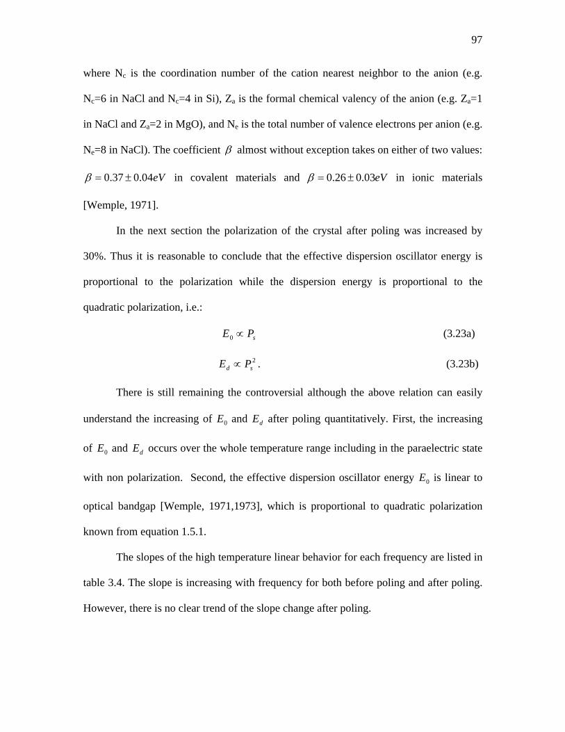
97
where Nc is the coordination number of the cation nearest neighbor to the anion (e.g.
Nc=6 in NaCl and Nc=4 in Si), Za is the formal chemical valency of the anion (e.g. Za=1
in NaCl and Za=2 in MgO), and Ne is the total number of valence electrons per anion (e.g.
Ne=8 in NaCl). The coefficient β almost without exception takes on either of two values:
eV04.037.0 ±=β in covalent materials and eV03.026.0 ±=β in ionic materials
[Wemple, 1971].
In the next section the polarization of the crystal after poling was increased by
30%. Thus it is reasonable to conclude that the effective dispersion oscillator energy is
proportional to the polarization while the dispersion energy is proportional to the
quadratic polarization, i.e.:
sPE ∝0 (3.23a)
2sd PE ∝ . (3.23b)
There is still remaining the controversial although the above relation can easily
understand the increasing of 0E and dE after poling quantitatively. First, the increasing
of 0E and dE occurs over the whole temperature range including in the paraelectric state
with non polarization. Second, the effective dispersion oscillator energy 0E is linear to
optical bandgap [Wemple, 1971,1973], which is proportional to quadratic polarization
known from equation 1.5.1.
The slopes of the high temperature linear behavior for each frequency are listed in
table 3.4. The slope is increasing with frequency for both before poling and after poling.
However, there is no clear trend of the slope change after poling.
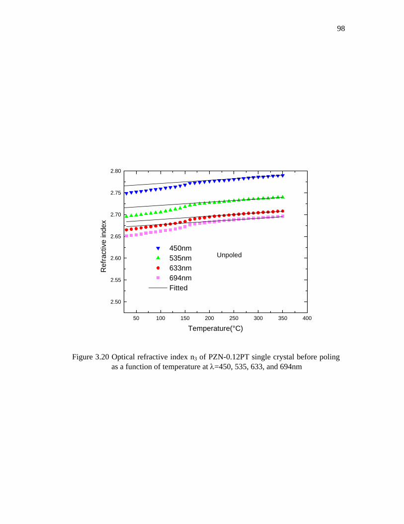
98
50 100 150 200 250 300 350 400
2.50
2.55
2.60
2.65
2.70
2.75
2.80
Unpoled
450nm 535nm 633nm 694nm Fitted
Ref
ract
ive
inde
x
Temperature(°C)
Figure 3.20 Optical refractive index n3 of PZN-0.12PT single crystal before poling as a function of temperature at λ=450, 535, 633, and 694nm
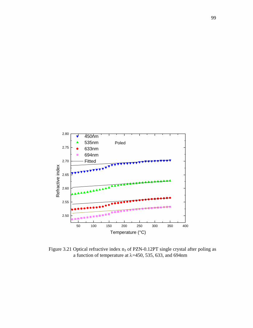
99
50 100 150 200 250 300 350 400
2.50
2.55
2.60
2.65
2.70
2.75
2.80
Poled
450nm 535nm 633nm 694nm Fitted
Ref
ract
ive
inde
x
Temperature (°C)
Figure 3.21 Optical refractive index n3 of PZN-0.12PT single crystal after poling as a function of temperature at λ=450, 535, 633, and 694nm
100
0 50 100 150 200 250 300 350 400
6.0
7.5
8.0
unpoled poled
E g (eV
)
Temperature (C°)
Figure 3.22 Temperature dependent effective dispersion oscillator energy E0
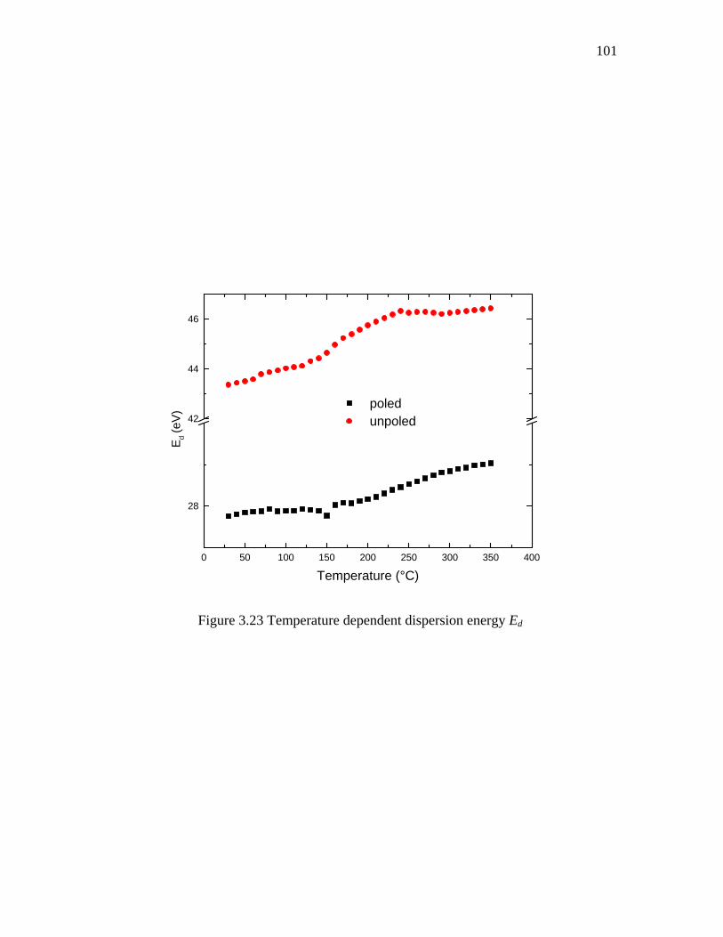
101
0 50 100 150 200 250 300 350 400
28
42
44
46
Ed (
eV)
poled unpoled
Temperature (°C)
Figure 3.23 Temperature dependent dispersion energy Ed
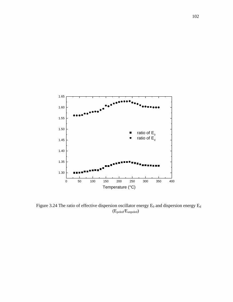
102
0 50 100 150 200 250 300 350 400
1.30
1.35
1.40
1.45
1.50
1.55
1.60
1.65
ratio of E0 ratio of Ed
Temperature (°C)
Figure 3.24 The ratio of effective dispersion oscillator energy E0 and dispersion energy Ed (Epoled/Eunpoled)
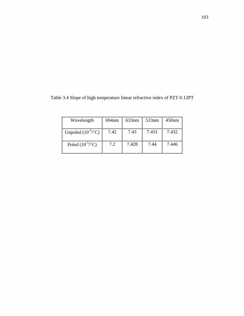
103
Table 3.4 Slope of high temperature linear refractive index of PZT-0.12PT
Wavelength 694nm 633nm 533nm 450nm
Unpoled (10-5/°C) 7.42 7.43 7.431 7.432
Poled (10-5/°C) 7.2 7.428 7.44 7.446
104
3.4.3 Birefringence of PZN-0.12PT
Birefringence PZN-0.12PT was measured at wavelength of 694nm, 633nm, and
535nm as shown in Figure 3.25. The higher the frequency of the light, the larger the
birefringence. All three birefringence remained negative in the measurement temperature
range. In the temperature above 200°C, due to the small view field of the lens and
limitation of equation 3.15, the birefringence is not reliable when the value is less than
0.005. Since during this temperature range the number of fringes (less than 1 within the
filed of view) was almost still, birefringence was estimated as constants. The accurate
measurement of birefringence for this temperature range will be introduced in chapter 6.
3.4.4 Polarization of PZN-0.12PT
The polarizations of PZN-0.12PT were calculated from both data set of refractive
index and birefringence. From the result of refractive index the polarization after poling
is about 0.4C/m2, which is in agreement with the result of [Lu 2000] and [Kuwata 1982].
Also the polarization is improved 30% after poling. The polarization derived from the
birefringence is slightly larger than the one from refractive index. As mentioned in the
last section the measured birefringence above 200 °C was approximated as constant;
although in fact there is a small positive trend of the birefringence with temperature. Thus
the value of )( 31nΔδ in equation 3.10 for calculation was larger than the real one, and
this caused slightly upper bound estimation on polarization. Here
241211 /013.0 Cmgg =− [Kuwata 1982].
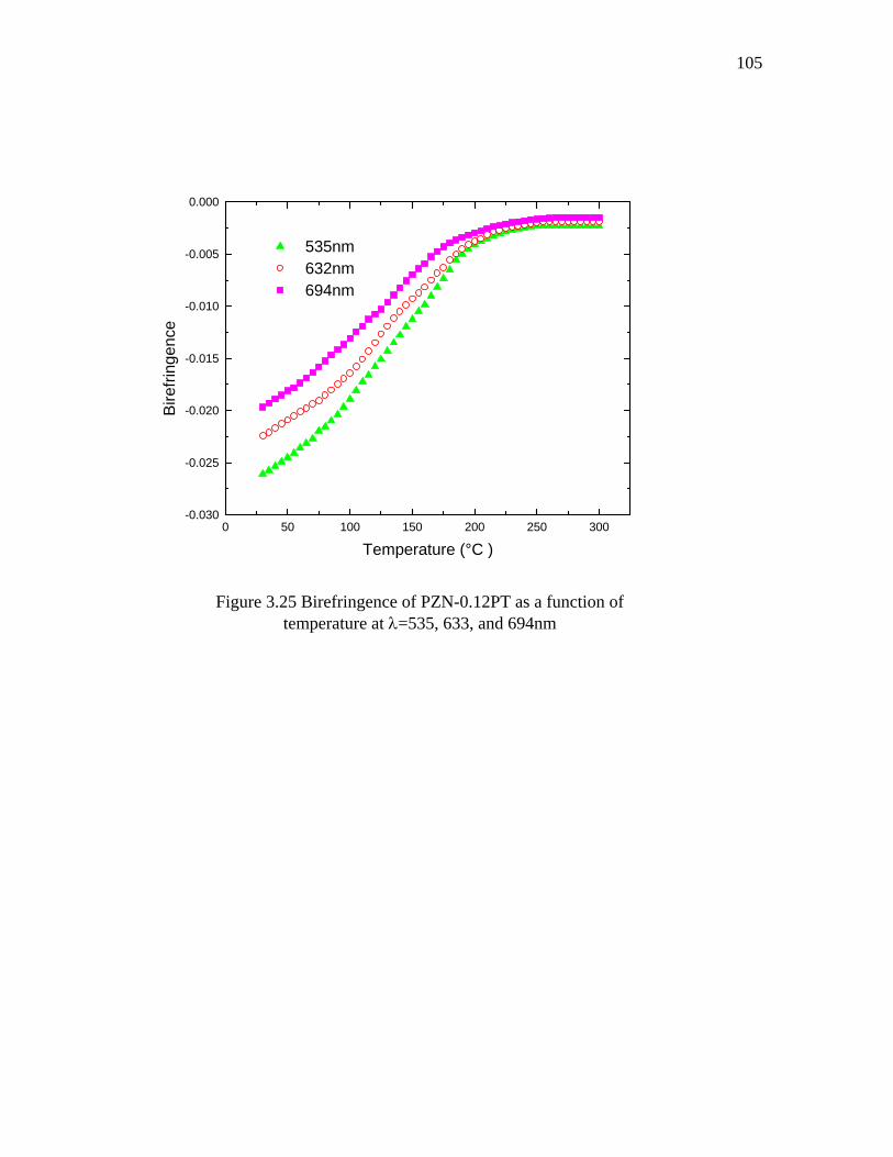
105
0 50 100 150 200 250 300-0.030
-0.025
-0.020
-0.015
-0.010
-0.005
0.000
535nm 632nm 694nm
Bire
fring
ence
Temperature (°C )
Figure 3.25 Birefringence of PZN-0.12PT as a function of temperature at λ=535, 633, and 694nm
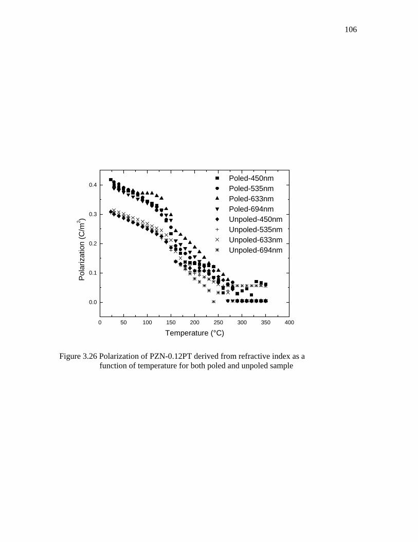
106
0 50 100 150 200 250 300 350 400
0.0
0.1
0.2
0.3
0.4
Poled-450nm Poled-535nm Poled-633nm Poled-694nm Unpoled-450nm Unpoled-535nm Unpoled-633nm Unpoled-694nm
Pola
rizat
ion
(C/m
2 )
Temperature (°C)
Figure 3.26 Polarization of PZN-0.12PT derived from refractive index as a function of temperature for both poled and unpoled sample
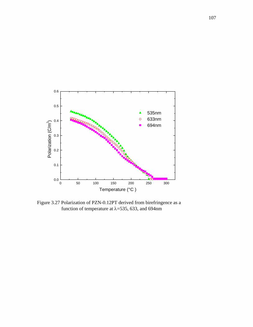
107
0 50 100 150 200 250 3000.0
0.1
0.2
0.3
0.4
0.5
0.6
535nm 633nm 694nm
Pola
rizat
ion
(C/m
2 )
Temperature (°C )
Figure 3.27 Polarization of PZN-0.12PT derived from birefringence as a function of temperature at λ=535, 633, and 694nm
108
108
Chapter 4
Thermo-optical properties
4.1 Introduction
The temperature dependence of the refractive index dTdn of ferroelectrics is of
practical importance in many optical and optoelectronic applications such as in focusing,
guiding, coupling, modulation of radiation, optical fiber communication system, and
high-resolution photographic lenses, which are required to operate under a wide range of
temperature conditions [Tsay 1973]. When the crystal is used in laser applications, it will
absorb part of the Laser power and be heated, and in turn the refractive index is changed.
By changing the ambient temperature the refractive index also can be varied. In some
other applications, both the absolute magnitude of dTdn , as well as its frequency
dependence are of interest, such as nonlinear crystal in the high-power nonlinear optical
device [Ghosh 1994, 1995].
Usually there are two aspects ascribing to dTdn coefficient for common
dielectric. One comes from thermal expansion; when temperature increases, the material
expands, becoming less dense. This mechanism would tend to make dTdn negative.
Another is the dependence of dipole moment on ionic displacements or the so-called
electron-phonon interaction. In addition, however, the polarization contribution must be
considered in ferroelectrics thus the expression below contains three terms:
)()()( PdTdnE
dTdn
dTdn
dTdn
g ++= α (4.1)
The first contribution can be expressed by using thermal expansion coefficient. As to the
second contribution, no uniform formula is available until now. Most literatures [Zysset
109
109
1992; Tsay 1973, 1977] attribute this contribution to the temperature change of bandgaps.
But Zhu et al.[Zhu 1987] pointed out that this was obscure. The optical refractive index is
related to the difference between the average energies of the conduction and valence
bands, rather than the bandgaps. Surely the bandgaps usually decrease with an increasing
temperature, but in the meantime bandwidths increase. Therefore, it is not straightforward
to decide whether the difference increases or decreases with the increasing temperature.
The last term corresponds to electrooptic effect due to the temperature dependent
spontaneous polarization, Ps.
4.2 Experiment results
From the measured optical refractive index and birefringence presented in chapter
3, the thermo-optical coefficients for a given frequency are determined and approximated
by the differential:
12
12 )()(TT
TnTndTdn
−−
= (4.2)
4.2.1 Thermo optical properties of PBN
The thermo-optic coefficients of n3 and (n3 -n1) for PBN obtained from the
refractive index n3 and birefringence are shown in Figure 4.1 and Figure 4.2 respectively.
The thermo-optic coefficients of n3 show strong temperature and frequency dependence
below Td but weak frequency dispersion at temperature above Td as shown in Figure 4.1.
The calculated thermo-optic coefficients of the birefringence (in Figure 4.2) also
show strong temperature dependence but weak frequency dispersion compared to that of
refractive index n3. By comparing the thermo-optic coefficient of n3 and birefringence of
535nm at discrete temperature (values summarized in Table 4.1), the thermo-optic
coefficient of n1 is derived. As can be seen the thermo-optic coefficients of n1 are much
110
110
less than those of n3 at low temperature range. It has been observed that n1 is much less
dependent on temperature compared to n3 for tetragonal ferroelectrics PBN [Guo t al.,
1990] and SBN [Bhalla et al., 1987, 1992] with tungsten bronze structure. This confirms
that polarizability is highly anisotropic with primary contribution coming from the ionic
longitudinal displacement parallel to c-axis. At the high temperature range the slope of
the birefringence increases with frequency
The first electronic term in equation 4.1 is usually positive since Eg decreases with
temperature and has an order of 10-5 for ionic crystal. The second lattice term is negative
for thermal expansion and positive for thermal contraction because the electronic
polarization density is proportional to the density of the material and has an order of 10-5
for ionic crystal [Tsay 1973]. The last polarization term can be the main contribution for
ferroelectrics. In the high temperature paraelectric state, there is no significant change of
n3. This should be due to the compensation of positive electronic term and negative
lattice term and both of them are around 10-5. While in low temperature ferroelectric
state, the lattice term is positive due to the contraction of x3 which increases with
temperature [Bhalla et al., 1987, 1992], thus in the ferroelectric state all three terms are
positive. The polarization term can be of the order of 10-4 at ferroelectric phase, e.g. at
180°C. In the high temperature paraelectric state, the n1 decreases with temperature. This
is similar as that of SBN of tetragonal tungsten bronze structure. The lattice term of n1 is
negative during all the temperature range unlike the one of n3. The negative thermo-optic
coefficient of paraelectric state implies that the electronic term is not enough to
compensate the lattice expansion effect. Comparing thermo-optic coefficients in low
temperature ferroelectric state and in high temperature paraelectric state, one can
111
111
conclude that there is a positive contribution of polarization term in ferroelectric state
with an order of 10-5. Comparing the polarization term of n3 and n1 in ferroelectric state,
the conclusion obtained again indicates that 33g is much lager than 13g from equations
3.8 and 3.9.
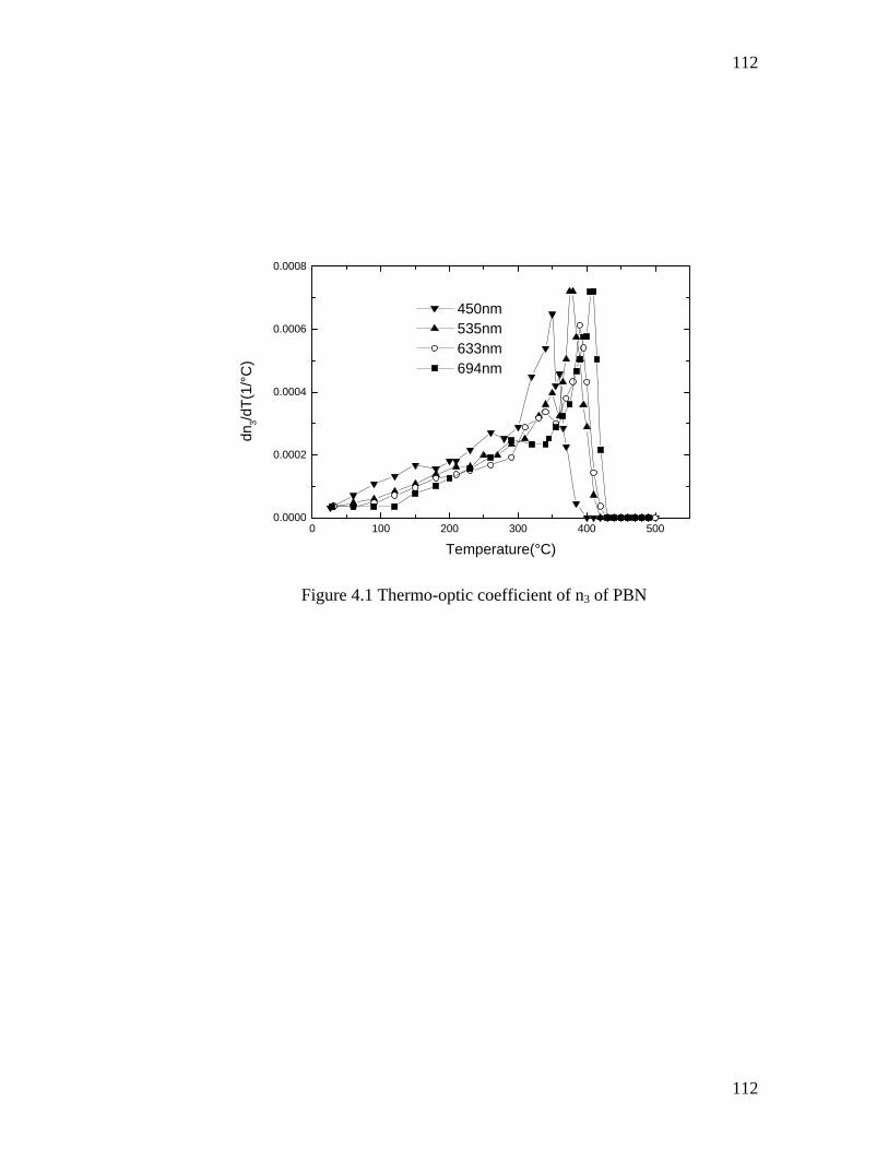
112
112
0 100 200 300 400 5000.0000
0.0002
0.0004
0.0006
0.0008
450nm 535nm 633nm 694nm
dn3/d
T(1/
°C)
Temperature(°C)
Figure 4.1 Thermo-optic coefficient of n3 of PBN

113
113
0 100 200 300 400 5000.0000
0.0002
0.0004
0.0006
0.0008
535nm 633nm 694nm
dΔn 31
/dT
(1/°
C )
Temperature (°C)
Figure 4.2 Thermo-optic coefficient of birefringence of PBN
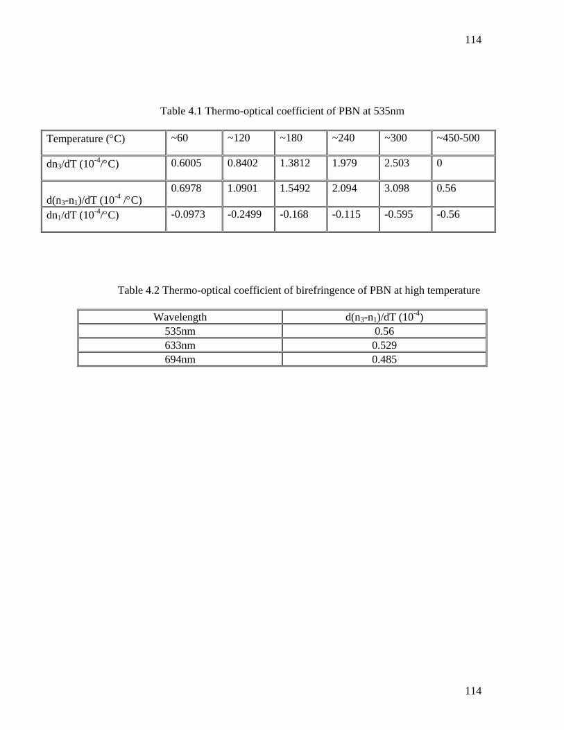
114
114
Table 4.1 Thermo-optical coefficient of PBN at 535nm
Temperature (°C) ~60 ~120 ~180 ~240 ~300 ~450-500
dn3/dT (10-4/°C) 0.6005 0.8402 1.3812 1.979 2.503 0
d(n3-n1)/dT (10-4 /°C) 0.6978 1.0901 1.5492 2.094 3.098 0.56
dn1/dT (10-4/°C) -0.0973 -0.2499 -0.168 -0.115 -0.595 -0.56
Table 4.2 Thermo-optical coefficient of birefringence of PBN at high temperature
Wavelength d(n3-n1)/dT (10-4) 535nm 0.56 633nm 0.529 694nm 0.485
115
115
4.2.2 Thermo optical properties of PZN-0.12PT
The thermo-optic coefficients of n3 for PZN-0.12PT before and after poling are
shown in Figure 4.3 and 4.4, respectively. The thermo-optic coefficients of (n3 -n1) are
plotted in Figure 4. The thermo-optic coefficients of n3 for PZN-0.12PT are similar to
PBN also exhibiting temperature and frequency dependence below Tm (around 160°C)
but weak frequency dispersion at temperature above Tm (see Table 3.4). It's evident that
after poling the thermo-optic coefficients of n3 in the low temperature range increased. As
discussed before, this is also due to the polarization term in equation 4.1. After poling the
polarization increased by 30% for PZN-0.12PT crystal and this increased polarization
improved the thermo-optic coefficients consequently. Unlike PBN57 with negative
thermo-optic coefficients of n1 in ferroelectric state, the thermo-optic coefficients of n1 of
PZN-0.12PT are positive in ferroelectric state.
The thermo-optic behavior can be analysis in terms of temperature dependent
single oscillator parameters, 0E and dE . In differential form equation 3.16 becomes
[Wemple, 1977]:
⎟⎟⎠
⎞⎜⎜⎝
⎛ ++−
⎟⎟⎟⎟
⎠
⎞
⎜⎜⎜⎜
⎝
⎛−
−= 20
20
22 )1()1(2
)1(E
EKKEdTdE
nn
dTdn
d
(4.3a)
where,
dTEd
dTEd
Kd
0ln
ln
= (4.3b)
The quantity K depends on the detailed shape of the imaginary part of the
dielectric constant spectrum 2ε and its temperature dependence. For a linear energy shift
with temperature of this entire spectrum without distortion, it can be shown that
116
116
10 ≤≤ K and the precise value dependence on details of the spectral shape. For 1>K , it
is necessary that the 2ε spectrum change shape as well as shift position with temperature.
The value 1=K forms a boundary between situations where the magnitude of
dTdn / increases or decreases as the photon energy approaches the interband dege. The
latter situation also allows for a change in sign of dTdn / as a function of optical
wavelength. The decreasing of the bandgap parameter 0E implies that the levels of
transition to the valence band are reduced while the positive dE suggests that the strength
of those energy levels closest to the band edge are also changing to increased strength
and broadening of the optical oscillator transition resonances. The large value of
dTdE /0 has also been noted to be associated with a very small coefficient of thermal
expansion in materials.

117
117
0 50 100 150 200 250 300 350 4000.0000
0.0001
0.0002
0.0003
0.0004
0.0005
Unpoled
450nm 535nm 633nm 694nm
dn3/d
T
Temperature (Cº)
Figure 4.3Thermo-optic coefficient of n3 of unpoled PZN-0.12PT sample
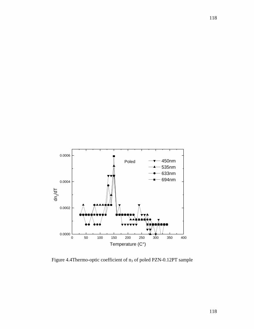
118
118
0 50 100 150 200 250 300 350 4000.0000
0.0002
0.0004
0.0006
Poled
450nm 535nm 633nm 694nm
dn3/d
T
Temperature (C°)
Figure 4.4Thermo-optic coefficient of n3 of poled PZN-0.12PT sample
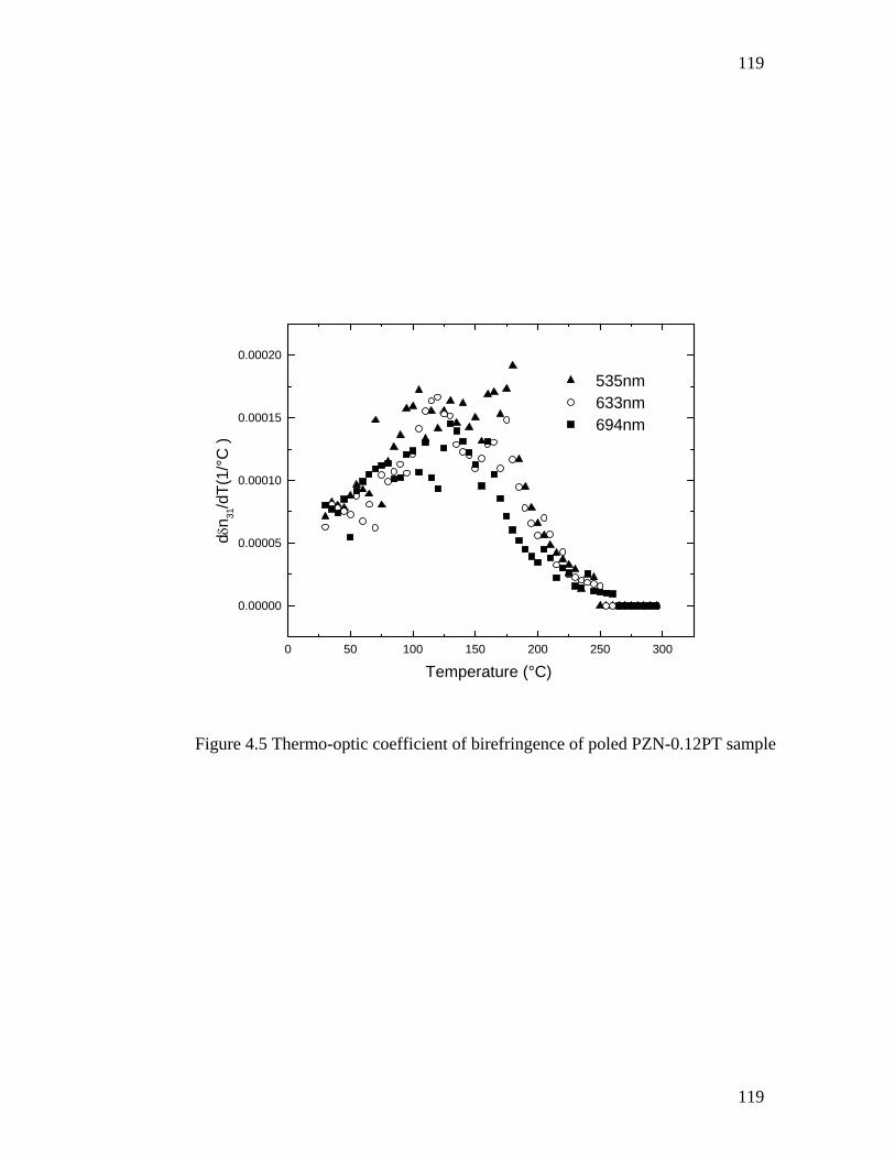
119
119
0 50 100 150 200 250 300
0.00000
0.00005
0.00010
0.00015
0.00020
535nm 633nm 694nm
dδn 31
/dT(
1/°C
)
Temperature (°C)
Figure 4.5 Thermo-optic coefficient of birefringence of poled PZN-0.12PT sample
120
Chapter 5
Transmission spectrum analysis
5.1 Introduction
The optical transmission spectrum study can reveal the information about the
electronic band structure, fundamental optical bandgap, ionic lattice absorption, and
material impurities of the sample. is of fundamental important. As a relaxor system PZN-
PT, it is also interesting to examine how the poling causes the optical bandgap shift, the
effects of electron-phonon interaction, as well as the optical anisotropic properties.
5.1.1 Transmission spectrum measurement system
The PC2000-UV-VIS Miniature Fiber Optic Spectrometer (Ocean Optics Inc.)
was used to measure the transmission spectrum. The transmission spectrum was collected
by the software OOIbase 32. In order to obtain a transmission spectrum, a dark spectrum
(D), which is the spectrum after blocking the light source, reference spectrum (R), which
is the spectrum without sample, and sample spectrum (S) are measured. Then the
transmission spectrum (T) is calculated by:
%100)()()()()( ×
−−
=λλλλλ
DRDST (5.1)
5.1.2 Fourier transform Infrared spectroscopy
The Nicolet-6700FT-IR spectrometer ( Thermo Electron Corp.) was used to
measure the FTIR spectrum. Fourier Transform Infrared spectroscopy (FTIR) is a
measurement technique for collecting infrared spectra. Instead of recording the amount of
energy absorbed when the frequency of the infra-red light is varied (monochromator), the
IR light is guided through an interferometer. After passing the sample the measured
121
signal is in form of its interferogram. Performing a mathematical Fourier Transform on
this signal results in a spectrum identical to that from conventional (dispersive) infrared
spectroscopy.
FTIR spectrometers are cheaper than conventional spectrometers because building
of interferometers is easier than the fabrication of a monochromator. In addition,
measurement of single spectra is faster for the FTIR technique because the information of
all frequencies is collected simultaneously. This allows multiple samples to be collected
and averaged together resulting in an improvement in sensitivity. Because of its various
advantages, virtually all modern infrared spectrometers are of the FTIR variety.
5.2 Experiment and results
Optical quality PZN-0.12PT single crystal with dimension 32.065.22.4 ×× mm
was studied both before and after poling. The same poling procedure as applied to the
sample used for index measurement was applied to this sample. Spectra were measured
both prior and after poling along a axis and c axis with a polarizer at room temperature.
5.2.1 Results of transmission spectrum
5.2.1.1 Transmission spectrum
The measured transmission spectra from 350nm to 1000nm were shown in Figure
5.1. Before poling, transmissions of both spectra along a-axis and along c-axis are around
30%. While after poling, transmissions are improved dramatically to around 60%. On the
surface and domain walls of the crystal sample, the optical refractive index is
discontinuous to result in reflection loss and less transmission. The unpoled sample has
much more domains (walls) and nanoregions with different orientation with respect to the
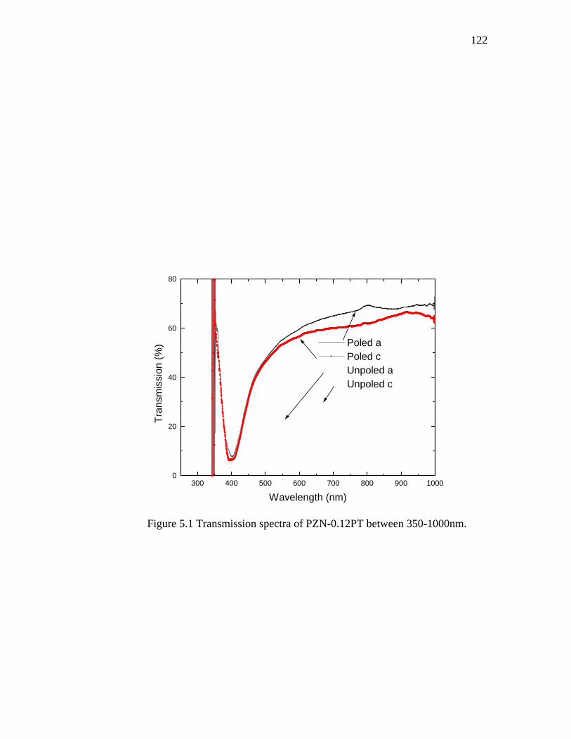
122
300 400 500 600 700 800 900 10000
20
40
60
80
Poled a Poled c Unpoled a Unpoled c
Tran
smis
sion
(%)
Wavelength (nm)
Figure 5.1 Transmission spectra of PZN-0.12PT between 350-1000nm.
123
optical axis comparing with the poled sample. Thus when the light passes through the
unpoled crystal, those domain walls cause large reflection loss or scattering loss. For
PZN-0.12PT single crystal, after poling along the <001> direction, the single domain area
enlarges and the loss due to domain walls reduced significantly. There is a very slight
difference of the transmission along a axis and c axis of the unpoled sample indicating
that the unpoled sample is almost isotropic. This is in agreement with the fact that the
pseudo-cubic structure of unpoled PZN-0.12PT. While the evident difference of
transmission along a axis and c axis for the poled sample is also verifying the anisotropic
structure of poled sample.
5.2.1.2 Absorption coefficient
In chapter 1 equation 1.5.17 gives the general case when light passes through a
sample. While for a sample of parallel plate form this equation is necessary to be
corrected after considering the reflection and multi-reflection in the sample as shown in
Figure 5.2. The reflection of the surface between the sample and air is 2
11⎟⎠⎞
⎜⎝⎛
+−
=nnR , n
the refractive index of the sample. Light with intensity 0I indent on the sample, the first
order transmission light intensity is deIR α−− 02)1( , the second order is deIRR α3
022 )1( −− ,
and so on. So the total transmission light intensity is summed as:
d
dddd
eReRIeReReRII α
αααα
22
2044222
0 1)1()1()1( −
−−−−
−−
=+++−= L . (5.2)
The transmission is given by:
d
d
eReR
IIT α
α
22
2
0 1)1(
−
−
−−
== . (5.3)
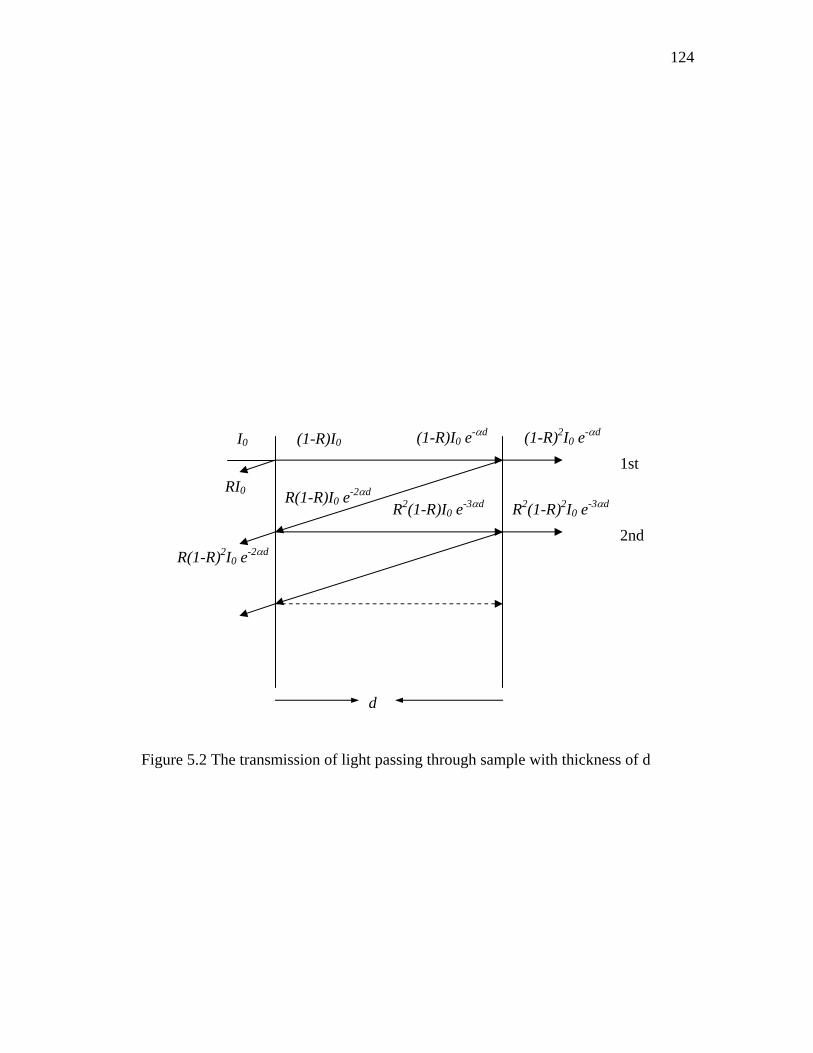
124
I0
RI0
(1-R)I0 (1-R)I0 e-αd (1-R)2I0 e-αd
R(1-R)I0 e-2αd
R(1-R)2I0 e-2αd
R2(1-R)I0 e-3αd R2(1-R)2I0 e-3αd
1st
2nd
d
Figure 5.2 The transmission of light passing through sample with thickness of d
125
The reflection is very weak dependent on the frequency in the visible range
though the refractive index is dependent on frequency. For both poled sample and
unpoled sample, the difference of reflection of 450nm and 694nm are both less than 2
percent. This ensures that the error can be omitted if taking reflection R as a constant in
equation 5.3. The absorption coefficients are calculated by equation 5.3 while R are both
taken as values of 535nm for poled sample and unpoled sample as shown in Figure 5.3.
The absorption coefficients cα are larger than aα for both poled sample and unpoled
sample. This will be discussed late.
5.2.1.3 Optical energy gap
As introduced in section 1.5.5, for indirect allowed transition the ωωα h)( vs.
ωh curve can consist of some straight lines and the adjacent two straight lines signify the
absorption and emission of phonons in certain state phonons as shown in Figure 1.12.
There is an obvious inflection point around 2.75 eV that separates the curve into two parts
with different slope. A linear fitting was applied to the curve near this region to yield two
straight lines with different slope as shown in Figure 5.4. The linear fitting data was
limited in a narrow region around 0.15 eV. The reason that such narrow region is chosen
rests on two considerations: firstly as introduced before that many state phonons are
involved in the transition, thus the linear fitting cannot be applied to the whole curve
otherwise only one state phonon will be yielded; secondly phonon energy are of the order
of 10 meV, the region of 0.15 eV is enough to yield one state phonon.
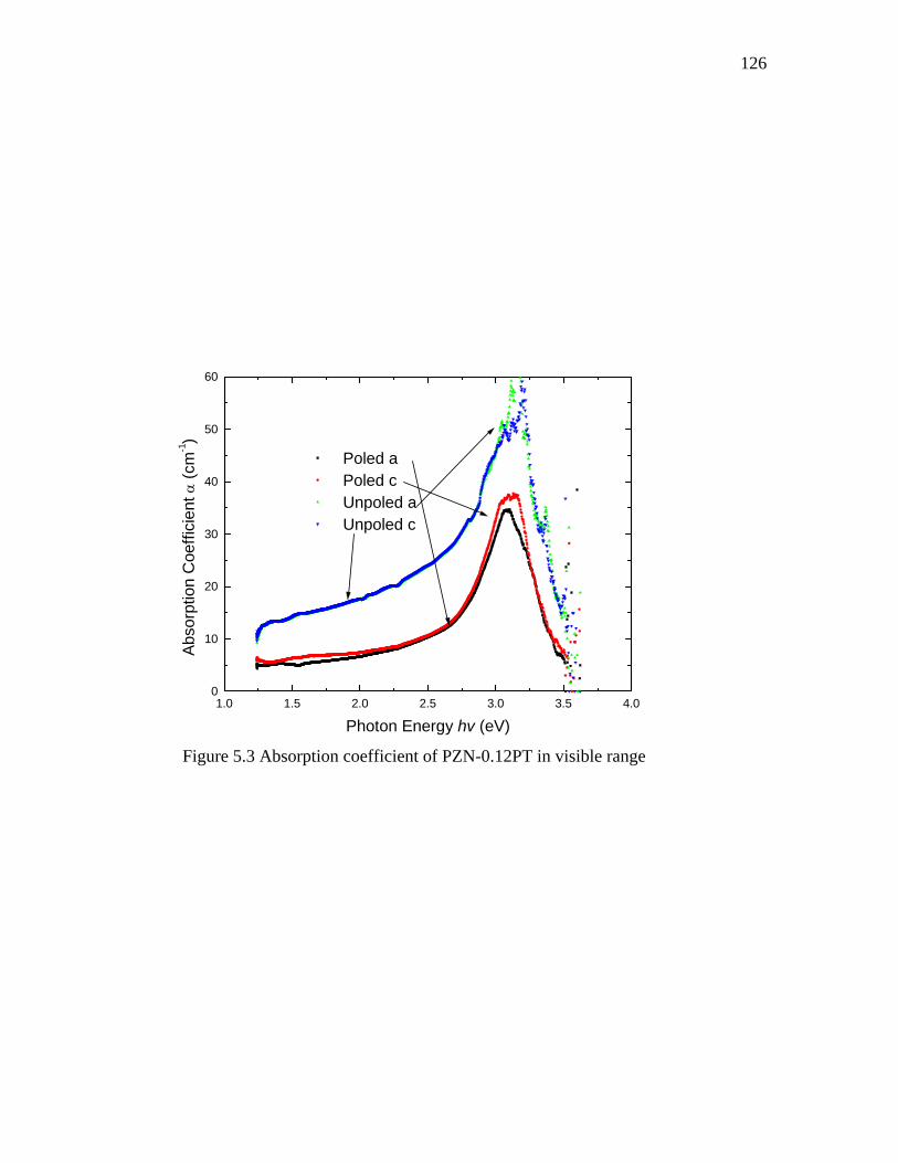
126
1.0 1.5 2.0 2.5 3.0 3.5 4.00
10
20
30
40
50
60
Poled a Poled c Unpoled a Unpoled c
Abso
rptio
n C
oeffi
cien
t α (c
m-1)
Photon Energy hv (eV)
Figure 5.3 Absorption coefficient of PZN-0.12PT in visible range
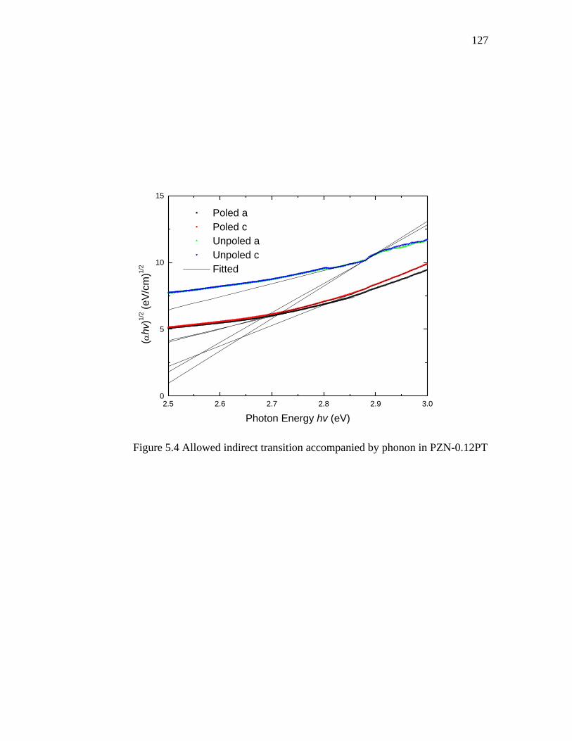
127
2.5 2.6 2.7 2.8 2.9 3.00
5
10
15
Poled a Poled c Unpoled a Unpoled c Fitted
(αhv
)1/2 (e
V/cm
)1/2
Photon Energy hv (eV)
Figure 5.4 Allowed indirect transition accompanied by phonon in PZN-0.12PT
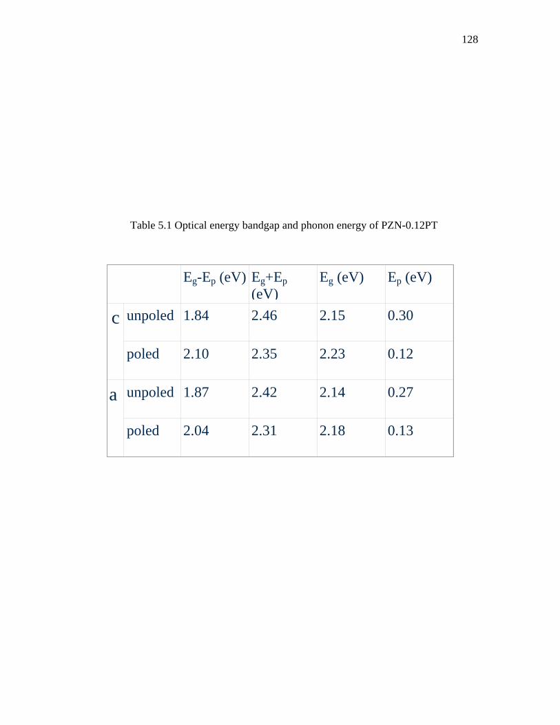
128
Eg-Ep (eV)
Eg+Ep (eV)
Eg (eV) Ep (eV)
c
unpoled
1.84 2.46 2.15 0.30
poled
2.10 2.35 2.23 0.12
a
unpoled
1.87 2.42 2.14 0.27
poled
2.04 2.31 2.18 0.13
Table 5.1 Optical energy bandgap and phonon energy of PZN-0.12PT
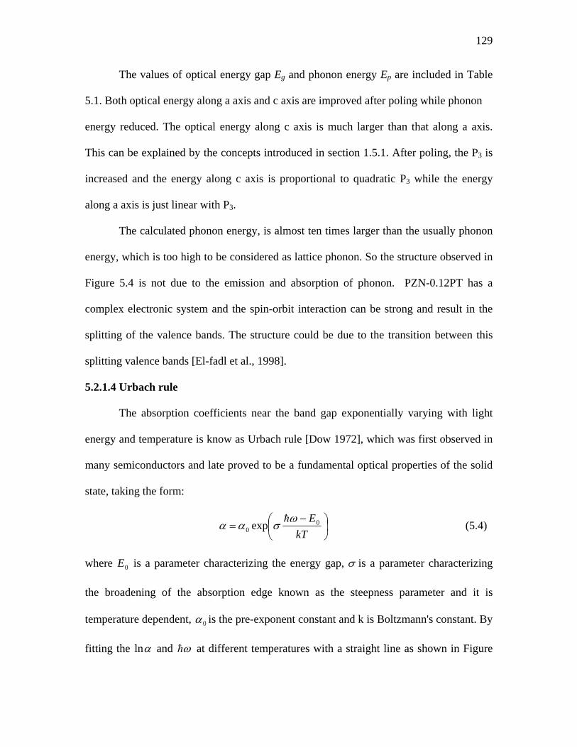
129
The values of optical energy gap Eg and phonon energy Ep are included in Table
5.1. Both optical energy along a axis and c axis are improved after poling while phonon
energy reduced. The optical energy along c axis is much larger than that along a axis.
This can be explained by the concepts introduced in section 1.5.1. After poling, the P3 is
increased and the energy along c axis is proportional to quadratic P3 while the energy
along a axis is just linear with P3.
The calculated phonon energy, is almost ten times larger than the usually phonon
energy, which is too high to be considered as lattice phonon. So the structure observed in
Figure 5.4 is not due to the emission and absorption of phonon. PZN-0.12PT has a
complex electronic system and the spin-orbit interaction can be strong and result in the
splitting of the valence bands. The structure could be due to the transition between this
splitting valence bands [El-fadl et al., 1998].
5.2.1.4 Urbach rule
The absorption coefficients near the band gap exponentially varying with light
energy and temperature is know as Urbach rule [Dow 1972], which was first observed in
many semiconductors and late proved to be a fundamental optical properties of the solid
state, taking the form:
⎟⎠⎞
⎜⎝⎛ −
=kT
E00 exp ω
σααh (5.4)
where 0E is a parameter characterizing the energy gap, σ is a parameter characterizing
the broadening of the absorption edge known as the steepness parameter and it is
temperature dependent, 0α is the pre-exponent constant and k is Boltzmann's constant. By
fitting the αln and ωh at different temperatures with a straight line as shown in Figure
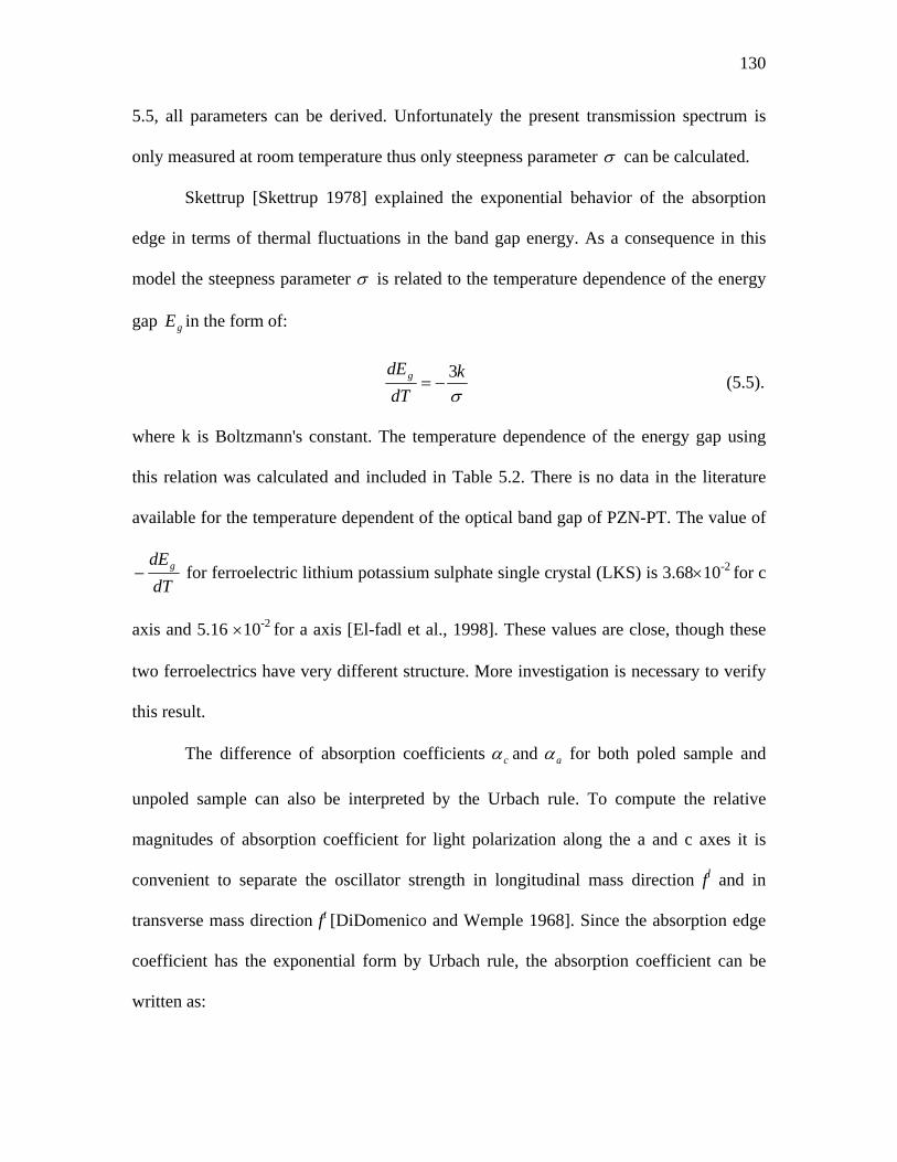
130
5.5, all parameters can be derived. Unfortunately the present transmission spectrum is
only measured at room temperature thus only steepness parameter σ can be calculated.
Skettrup [Skettrup 1978] explained the exponential behavior of the absorption
edge in terms of thermal fluctuations in the band gap energy. As a consequence in this
model the steepness parameter σ is related to the temperature dependence of the energy
gap gE in the form of:
σk
dTdEg 3
−= (5.5).
where k is Boltzmann's constant. The temperature dependence of the energy gap using
this relation was calculated and included in Table 5.2. There is no data in the literature
available for the temperature dependent of the optical band gap of PZN-PT. The value of
dTdEg− for ferroelectric lithium potassium sulphate single crystal (LKS) is 3.68×10⁻²
for c
axis and 5.16 ×10⁻² for a axis [El-fadl et al., 1998]. These values are close, though these
two ferroelectrics have very different structure. More investigation is necessary to verify
this result.
The difference of absorption coefficients cα and aα for both poled sample and
unpoled sample can also be interpreted by the Urbach rule. To compute the relative
magnitudes of absorption coefficient for light polarization along the a and c axes it is
convenient to separate the oscillator strength in longitudinal mass direction fl and in
transverse mass direction ft [DiDomenico and Wemple 1968]. Since the absorption edge
coefficient has the exponential form by Urbach rule, the absorption coefficient can be
written as:
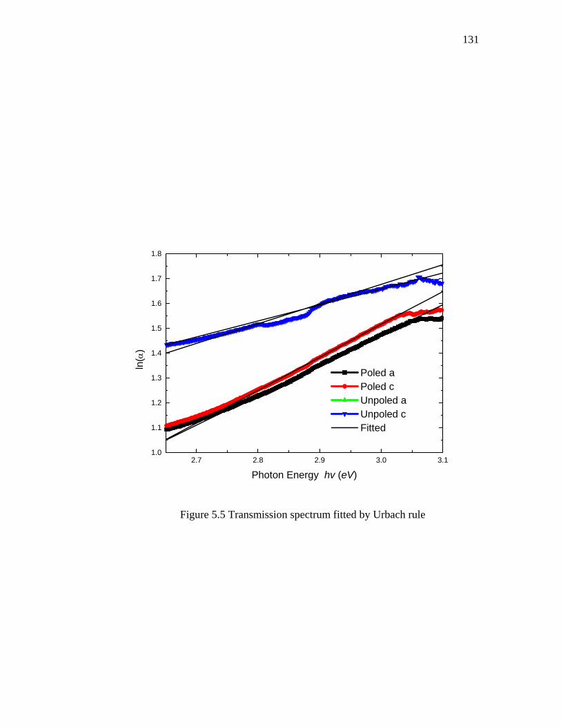
131
2.7 2.8 2.9 3.0 3.11.0
1.1
1.2
1.3
1.4
1.5
1.6
1.7
1.8
Poled a Poled c Unpoled a Unpoled c Fitted
ln(α
)
Photon Energy hv (eV)
Figure 5.5 Transmission spectrum fitted by Urbach rule
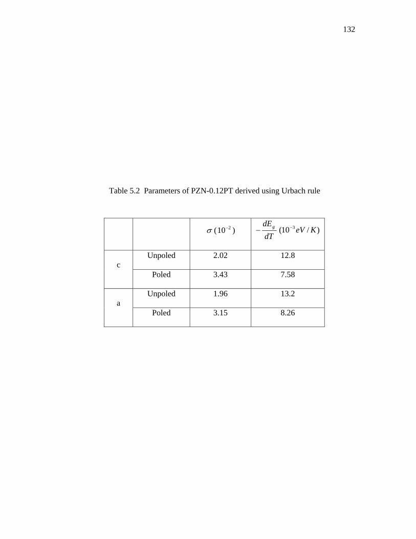
132
σ ( 210− ) dTdEg− )/10( 3 KeV−
Unpoled 2.02 12.8 c
Poled 3.43 7.58
Unpoled 1.96 13.2 a
Poled 3.15 8.26
Table 5.2 Parameters of PZN-0.12PT derived using Urbach rule
133
)](exp[ Ef ll −= ωβγα h (5.6a)
)](exp[ Ef tt −= ωβγα h (5.6b)
where γ is a constant of proportionality which includes the joint density of states, and
kTσβ = . Since longitudinal transition is much weaker than transverse, it is reasonable
to take 0=lα . The light will not "see" the transition when its direction is parallel to the
light polarization, thus when light polarization is parallel to the c axis only two
perpendicular directions, both along the a axis, count while light polarization parallel to
the a axis two perpendicular direction are along the c axis and another a axis for the
tetragonal structure. The anisotropic coefficients are obtained as:
)](exp[2 at
c Ehf −= νβγα (5.7a)
)])(exp[)]((exp[ cat
a EhEhf −+−= νβνβγα (5.7b)
where the oscillator strengths are assumed to be insensitive to the lattice polarization.
The ratio of the absorption coefficient along two directions is:
)](exp[12
caa
c
EE −+=
βαα (5.8).
For both poled and unpoled crystal, Ec is greater than Ea. So the value of equation 5.8 is
larger than 1.
5.2.2 Results of FTIR
The measured FTIR spectrums from 6500 cm-1 (15.4 μm) to 40000 cm-1 (2.5μm)
with resolution 2 cm-1 are show in Figure 5.6. The absorption is very strong when the
wavelength is above 5μm. After poling the transmission was improved to 35% from 15%
prior to poling. This is very similar as the transmission of the poled and unpoled sample
134
in the visible range. The reason is also due to the reflection and scattering loss resulting
from domain walls.
There are two strong absorption peaks for wavelength below 5μm as shown in
Figure 5.7. One absorption peak near 2.9 μm (3450cm-1) corresponds to the well-known
infrared absorption bands of O-H bond stretching mode. Hydrogen can easily enter the
crystal during the growth step, forming OH- radicals. The existence of hydroxyl ions
(OH-) has been reported in many ferroelectrics by IR absorption studies, such as SrTiO3
[Brebner et al., 1981; Houde et al., 1987], BatiO3 [Laulicht and Benguigui 1979;
Kapphan and Weber 1981], LiNbO3 [Herrington et al., 1973], SBN [Hunsche et al.,
1995], and PBN [Lee et al., 1996]. Protons (H+) play an essential role in thermal fixing
of stored hologram in LiNbO3 and PBN [Liu et al., 1997]. This indicates that it is
possible to use PZN-0.12PT for hologram application. Another absorption peak is around
3.4μm (2950cm-1). This corresponds to 365 meV, much large than any lattice phonon.
This could be due to a stretching mode of O-H bond but at a different site.
5.3 Summary
The transmission spectrum of PZN-0.12PT was measured in wavelength from
near UV 350nm to IR 15.4μm for both poled and unpoled samples with different
polarization directions. Transmission was improved significantly after poling due to the
supression scattering and reflection loss caused by domain walls. Optical band gap was
enlarged due to the increased polarization in the poled sample. The temperature
dependent optical band gap was determined by Urbach rule. The existence of Hydrogen
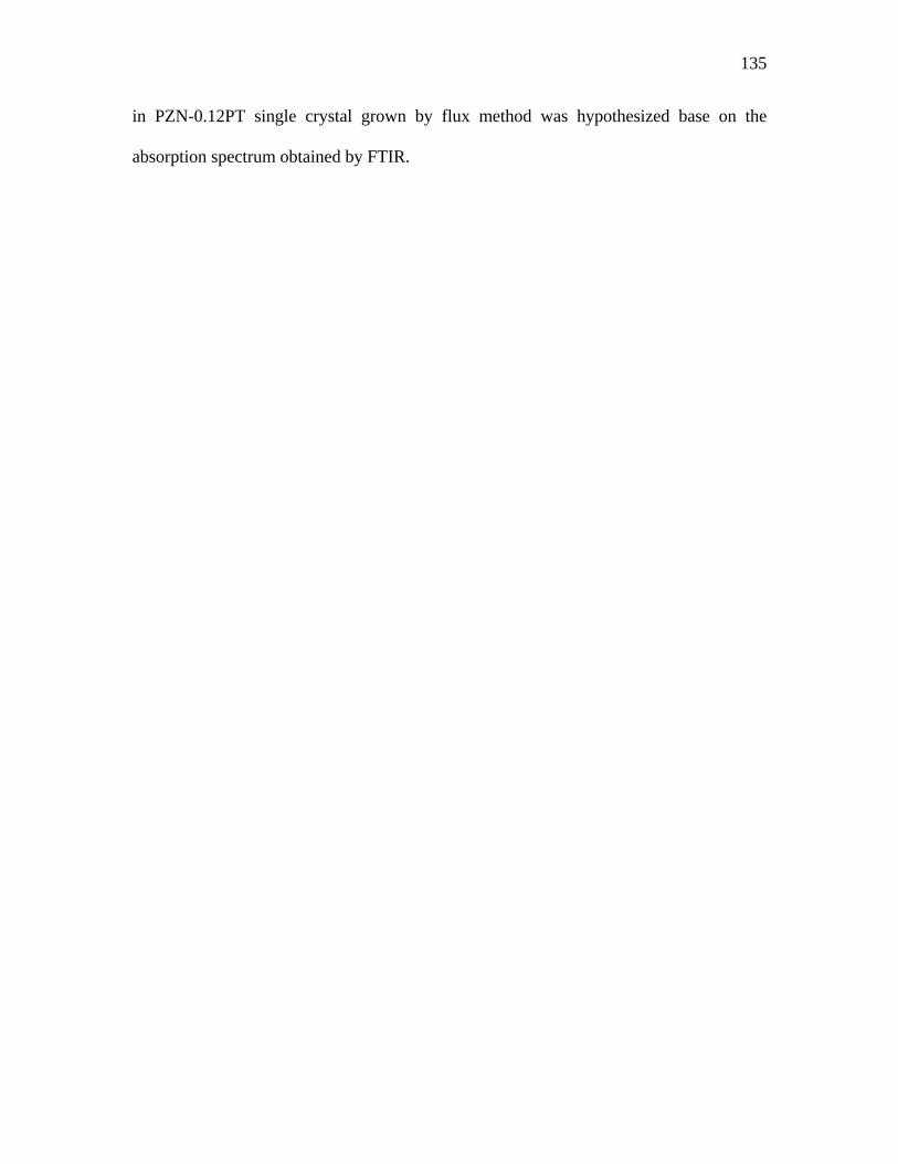
135
in PZN-0.12PT single crystal grown by flux method was hypothesized base on the
absorption spectrum obtained by FTIR.
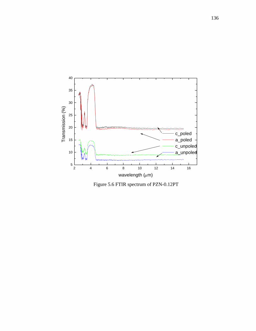
136
2 4 6 8 10 12 14 165
10
15
20
25
30
35
40
c_poled a_poled c_unpoled a_unpoled
Tran
smis
sion
(%)
wavelength (μm)
Figure 5.6 FTIR spectrum of PZN-0.12PT
137
2 3 4 55
10
15
20
25
30
35
40
c_poled a_poled c_unpoled a_unpoled
Tran
smis
sion
(%)
wavelength (μm)
Figure 5.7 Absorption peaks of PZN-0.12PT's FTIR spectrum
138
Chapter 6
Domain Configuration by Two
Dimensional Birefringence Measurement
6.1 Introduction
This chapter deals with the domain configuration as viewed by two dimensional
birefringence measurements. First it gives some basic concept of domain and Jones
matrix, which is the necessary mathematic tool for two-dimensional birefringence
measurement. It is followed by some preliminary test experiments and analysis.
6.1.1 Introduction on ferroelectric domains
Even for a single ferroelectric crystal, usually it does not consist only one domain,
since single domain corresponding to higher energy. Lowering the temperature of a
single crystal barium titanate with cubic symmetry (m3m) from above 130°C to below
Curie point, it has a tetragonal (4mm) symmetry. In this tetragonal state the polarization
axis (c axis) is not uniform in the whole crystal, but has six possible directions (three
cubic {100} axes. There are only two types of domains, i.e. 90° and 180°, since c axis is
originated from an a axis. At room temperature the optical refractive indices along a axis
and c axis have a difference 055.0)( =− ca nn . Due to this birefringence, it is possible to
observe the domains in it under transmitting polarized light since the domains are
separated by 90° walls,
Figure 6.1 shows a barium titanate single crystal in a ferroelectric state with two
domains. The c axis of domain I is Ic , and IIc for domain II. Cutting a plate section
perpendicular to AB near AC containing only Ic and set it between two-crossed
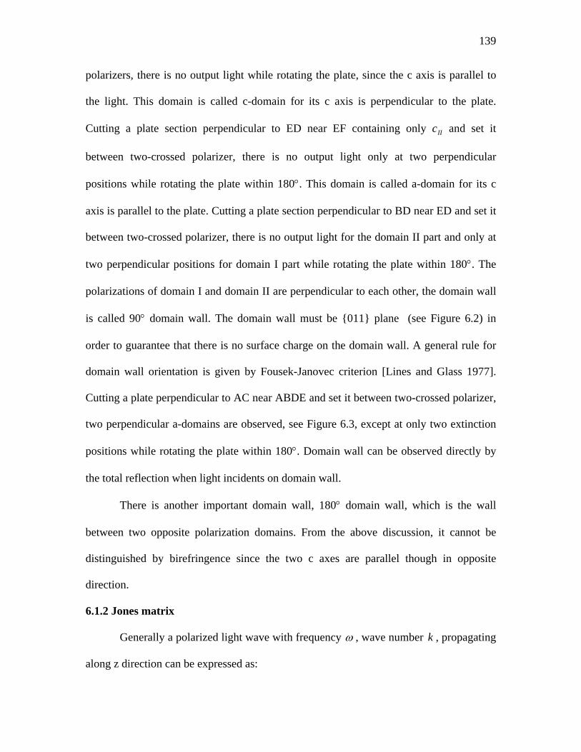
139
polarizers, there is no output light while rotating the plate, since the c axis is parallel to
the light. This domain is called c-domain for its c axis is perpendicular to the plate.
Cutting a plate section perpendicular to ED near EF containing only IIc and set it
between two-crossed polarizer, there is no output light only at two perpendicular
positions while rotating the plate within 180°. This domain is called a-domain for its c
axis is parallel to the plate. Cutting a plate section perpendicular to BD near ED and set it
between two-crossed polarizer, there is no output light for the domain II part and only at
two perpendicular positions for domain I part while rotating the plate within 180°. The
polarizations of domain I and domain II are perpendicular to each other, the domain wall
is called 90° domain wall. The domain wall must be {011} plane (see Figure 6.2) in
order to guarantee that there is no surface charge on the domain wall. A general rule for
domain wall orientation is given by Fousek-Janovec criterion [Lines and Glass 1977].
Cutting a plate perpendicular to AC near ABDE and set it between two-crossed polarizer,
two perpendicular a-domains are observed, see Figure 6.3, except at only two extinction
positions while rotating the plate within 180°. Domain wall can be observed directly by
the total reflection when light incidents on domain wall.
There is another important domain wall, 180° domain wall, which is the wall
between two opposite polarization domains. From the above discussion, it cannot be
distinguished by birefringence since the two c axes are parallel though in opposite
direction.
6.1.2 Jones matrix
Generally a polarized light wave with frequency ω , wave number k , propagating
along z direction can be expressed as:
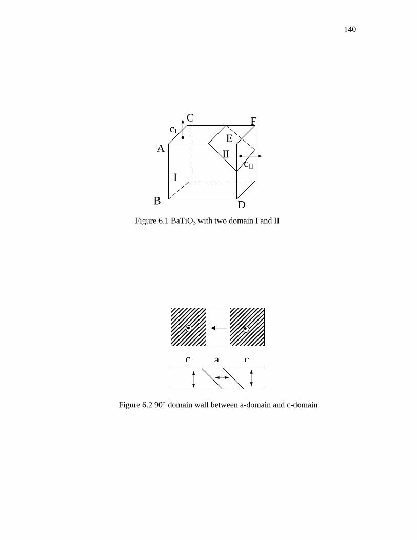
140
C
E
D B
F
II
I
cI
cII
A
Figure 6.1 BaTiO3 with two domain I and II
c a c
Figure 6.2 90° domain wall between a-domain and c-domain
141
jkztEikztEtzE xyxx )cos()cos(),( 00 φωφω +−++−= (6.1)
where xE0 , yE0 the amplitude of x, y component respectively.
Written in complex exponential form and omitting the time dependence by a
column notation, which is known as Jones vector [Kliger et al 1990]:
y
x
y
x
i
i
iy
ix
y
x
ee
EeEeE
EE
E φ
φ
φ
φ
αα
sincos
00
0 === (6.2)
where 20
200 yx EEE += , 00cos EE x=θ , and 00sin EE y=α
Only considering the linear interaction between light and the optical materials
when the light power or electric field intensity is not high enough. The final output light
can be described as:
yxfx EJEJE 1211 += (6.3.a)
yxfy EJEJE 2221 += (6.3.b)
where Jij are coefficients to be determined from the known properties of the optical
material encountered by the light. Using the Jones vector, equation (6.3) becomes:
y
x
fy
fx
EE
JJJJ
EE
2221
1211= (6.4)
where the matrix J is the so called Jones matrix.
The electric vector of a light wave that passes through an optical medium with
refractive index n and extinction coefficient κ is scaled by a factor of )(2
0κ
λπ indi
e−−
, where
d is the distance propagated in the medium and 0λ is the wavelength in vacuum. When a
polarized light passes through an optical medium with optical axis parallel to the light
electric field, i.e. x and y. Then equation (6.3) becomes:
142
xx
indi
xfx ENeEExx
==−− )(2
0κ
λπ
(6.5a)
yy
indi
yfy ENeEEyy
==−− )(2
0κ
λπ
(6.5b)
So the matrix representing a linear polarizer or retarder with optical axes oriented along
the a and y direction can be conclude as:
y
x
NN
J0
0)0( = (6.6)
where (0) denotes no rotation of the optical axes with respect to the coordinate axes. By
rotating the coordinate axes it is straightforward to get the matrix )(βJ for a linear
polarizer or retarder with its optical axes rotated by angel β (positive for
counterclockwise rotation from the x axis, see figure 6.4) from the coordinate.
)()0()()( βββ RJRJ −= (6.7)
where ββββ
βcossinsincos
)(−
=R (6.8)
For an ideal horizontal polarizer, the x component of the electric vector passes
without attenuation while the y component is attenuated completely. So 1=xN , 0=yN ,
thus,
0001
)0( =PJ (6.9)
The Jones matrix of a polarizer oriented at an angel β from the positive x axis
can be calculated directly by equation (6.7), (6.8), and (6.9),
ββββββ
β 2
2
sincossincossincos
)( =PJ (6.10)
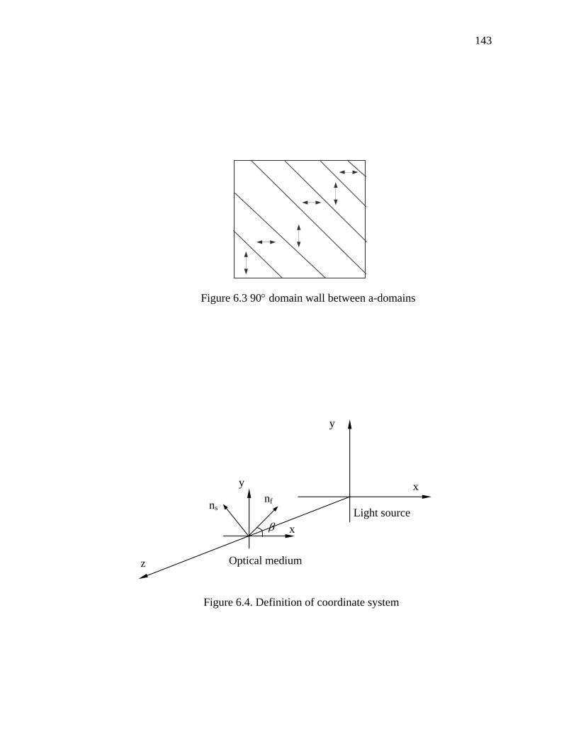
143
Figure 6.3 90° domain wall between a-domains
x
x
y
y
z
nf ns
β
Optical medium
Light source
Figure 6.4. Definition of coordinate system
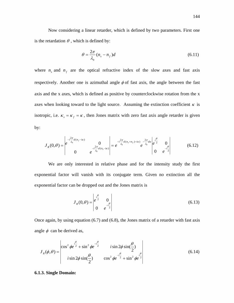
144
Now considering a linear retarder, which is defined by two parameters. First one
is the retardation θ , which is defined by:
dnn fs )(2
0
−=λπθ (6.11)
where sn and fn are the optical refractive index of the slow axes and fast axis
respectively. Another one is azimuthal angle φ of fast axis, the angle between the fast
axis and the x axes, which is defined as positive by counterclockwise rotation from the x
axes when looking toward to the light source. Assuming the extinction coefficient κ is
isotropic, i.e. κκκ == fs , then Jones matrix with zero fast axis angle retarder is given
by:
2
22))(2
)(2
)(2
0
0
0
0),0( 00
0
0
θ
θκ
λπκ
λπ
κλπ
κλπ
θi
idinndi
indi
indi
R
e
eeee
eJfx
s
f
−
−−+−
−−
−−
== (6.12)
We are only interested in relative phase and for the intensity study the first
exponential factor will vanish with its conjugate term. Given no extinction all the
exponential factor can be dropped out and the Jones matrix is
2
2
0
0),0( θ
θ
θi
i
R
e
eJ−
= (6.13)
Once again, by using equation (6.7) and (6.8), the Jones matrix of a retarder with fast axis
angle φ can be derived as,
2222
2222
sincos)2
sin(2sin
)2
sin(2sinsincos),( θθ
θθ
φφθφ
θφφφθφ
ii
ii
R
eei
ieeJ
+
+=
−
−
(6.14)
6.1.3. Single Domain:
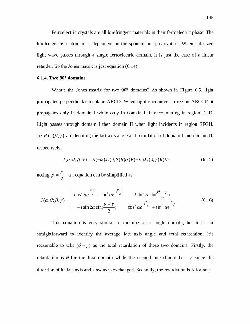
145
Ferroelectric crystals are all birefringent materials in their ferroelectric phase. The
birefringence of domain is dependent on the spontaneous polarization. When polarized
light wave passes through a single ferroelectric domain, it is just the case of a linear
retarder. So the Jones matrix is just equation (6.14)
6.1.4. Two 90° domains
What’s the Jones matrix for two 90° domains? As shown in Figure 6.5, light
propagates perpendicular to plane ABCD. When light encounters in region ABCGF, it
propagates only in domain I while only in domain II if encountering in region EHD.
Light passes through domain I then domain II when light incidents in region EFGH.
),( θα , ),( γβ are denoting the fast axis angle and retardation of domain I and domain II,
respectively.
)(),0()()(),0()(),;,( 21 βγβαθαγβθα RJRRJRJ −−= (6.15)
noting απβ +=2
, equation can be simplified as:
2222
2222
sincos)2
sin(2sin
)2
sin(2sinsincos),;,( γθγθ
γθγθ
ααγθα
γθαααγβθα −−
−
−−
−
+−
−
−−−
=ii
ii
eei
ieeJ (6.16)
This equation is very similar to the one of a single domain, but it is not
straightforward to identify the average fast axis angle and total retardation. It’s
reasonable to take )( γθ − as the total retardation of these two domains. Firstly, the
retardation is θ for the first domain while the second one should be γ− since the
direction of its fast axis and slow axes exchanged. Secondly, the retardation is θ for one
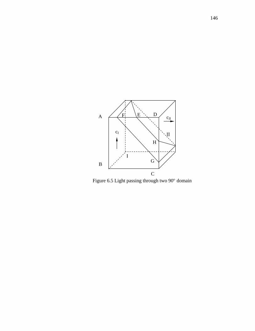
146
II
I
A
B
D
C
H
G
F E
cI
cII
Figure 6.5 Light passing through two 90° domain
147
domain while all the phase term containing 2θ in equation (14); while by
observing the phase factoring equation (16), they all contain the term of 2)( γθ − .
6.1.5. Three 90° domains
Now considering the Jones matrix of three 90° domains. Assuming that there is a
third 90° domain ),( σρ after that two 90° domain. 2πβρ ±= . For the case
of 2πβρ −= , then αρ = ,
)(),0()()(),0()()(),0()(),;,;,( 321 ρσρβγβαθασργβθα RJRRJRRJRJ −−−= (6.17)
Noting, 0110
)()()()(−
=−=− ρββα RRRR (6.18)
So, ),0()()(),0()()( 22 γρβγβα −−=−− JRRJRR (6.19)
And, ),0(),0(),0(),0( 3321 σγασγθ +−=− JJJJ (6.20)
Finally, ),(),;,;,( σγθασργβθα +−−= JJ (6.21)
For the case of 2πβρ += , then παρ += , the same result as equation (6.21) is
obtained. Since the light intensity is the measurement parameter in our experiment, the
minus sign can be omitted without affecting the results. So Jones matrix of three 90°
domains is
),(),;,;,( σγθασργβθα +−= JJ (6.22).
Unlike the case of two 90° domains, the total retardation and fast axis angle of
three 90° domains are easy to determine. The total retardation is σγθ +− , and the fast
axis angle is α , the same as the fast axis angle of the first domain. So three 90° domains
can be treated as a single domain ),( σγθα +− . Moreover, the total effect of odd 90°
148
domains can be treated as a single domain with the fast axis angle of α , the fast axis
angle of the first domain, and the retardation θ is
∑ +−=k
kk θθ 1)1( (6.23).
And then all the even 90° domains can be treated as two 90° domains.
6.2 Experimental Approach
6.2.1 System test
6.2.1.1. Measurement Principle and Setup
Figure 6.6 shows the fundamental setup of the rotating analyzer method for the
two-dimensional birefringence measurement. The actual arrangement of its optical
system is schematically drawn in Figure 6.7. An incident laser light passes through a
polarizer and a quarter-wave plate to generate a circularly polarized light and then
propagates through an uniaxial crystal under test. The relative phase shift θ is caused in
the uniaxial medium and the principal birefringence axis (i.e., the fast axis) has an angle
φ measured from the horizontal y axis. The Jones matrix representation of the output
light passing through an analyzer that is rotated by an angle Φ relative to the y axis is
given by [Ohmi 1994; Nishida and Yamanaka 2001]
⎥⎦
⎤⎢⎣
⎡⎥⎦
⎤⎢⎣
⎡⎥⎦
⎤⎢⎣
⎡
ΦΦΦΦΦΦ
=⎥⎦
⎤⎢⎣
⎡01
11
21),(
coscossincossinsin2
2
ii
JEE
Ry
x θφ (6.24),
),( θφRJ is given by equation (6.14).
The optical output intensity I is then straightforwardly obtained as
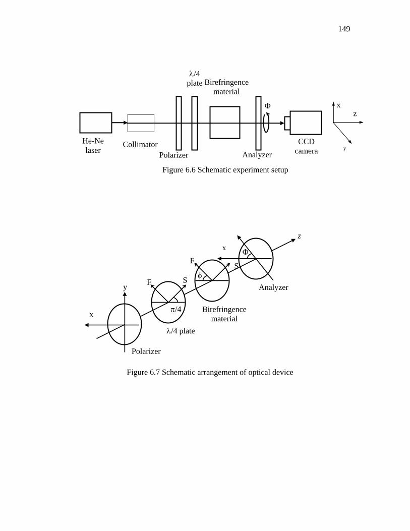
149
He-Ne laser Polarizer Analyzer
CCD camera
Birefringencematerial
λ/4 plate
Φ z
y
x
Collimator
Figure 6.6 Schematic experiment setup
Figure 6.7 Schematic arrangement of optical device
F
F
S
S
z x
y
π/4
φ
Φ
Polarizer
λ/4 plate
Birefringence material
Analyzer
x
150
( )[ ]θφ sin2sin12
22 −Φ−=+= oyx
IEEI , (6.25)
where Io is the incident intensity. A CCD camera detects the 2-D intensity data while the
analyzer is rotated about the axis of laser beam in steps of a fixed rotation angle. Then
calculations are carried out in a computer for each pixel of the captured image data and
the 2-D birefringence vector distribution ),( θφ in the sample is obtained simultaneously.
However, the rotation of the analyzer causes the additional change of the transmitted
intensity I regardless of performance of the optical measurement system characterized by
equation (6.25). In other words, the spatial nonuniformity of the analyzer resulting from
the production quality or some defects on its surfaces changes its optical transmittance
distribution at different rotation angles, which in turn lower the sensitivity of the 2-D
measurement depending on the optical characteristics of the analyzer. Therefore, the
transmitted intensity I at each pixel of the image data given by equation (6.25) can be
modified as
( )[ ]θφ sin2sin12
)(22 −Φ−Φ=+= o
yxITEEI (6.26)
Here )(ΦT accounts for the nonuniformity due to the analyzer rotation. It is a function of
Φ and its cancellation is required to improve the measurement sensitivity. To this end,
the rotating analyzer method is applied again without installing the uniaxial material to be
tested as shown in Figure 6.6.
2
)( oITI Φ= (6.27)
As shown in Figure 6.6, a He-Ne laser (632.8 nm) is used for an input light source
and a beam attenuator controls its intensity. The beam is collimated and passing through
151
the following polarizer and quarter-wave plate. Here a voltage-controllable nematic
liquid crystal retarder is used as the sample whose optical performance (i.e., the
retardation θ as a function of voltage) is obtained as shown in Figure 6.8. The
transmitted light intensity via the analyzer is recorded by the CCD camera and then sent
into the computer system for image processing to obtain the 2-D birefringence vector
distribution ),( θφ .
The procedure of measurement and image processing is as following. The first
step is to measure 19 intensity profile images from – 90° to 90° by 10° increments
without the sample in order to obtain )(ΦT effect given by equation (6.27). After
arranging the sample in the optical measurement system, the same measurement as that of
the first step is repeated to obtain the 2-D distribution of the retardation θ and the fast
axis direction φ in the nematic liquid crystal. Then all 36 intensity data are filtered out to
reduce the spatial noise and to remove dust or scratches in the intensity image. The
nonuniformity effect )(ΦT due to the rotation of the analyzer is compensated by dividing
the intensity data I measured without the sample at the same rotation angle Φ , and then
the birefringence vector distribution ),( θφ in the birefringence material can be calculated
by equation (6.26).
6.2.1.2 Experimental Results and Discussions
Original 2-D intensity images are taken by the CCD with changing the rotation
angle Φ of the analyzer under the experimental setup as shown in Figure 6.6. Each
captured image data has a total of 300 × 400 pixels with 8 bits of gray level. A square
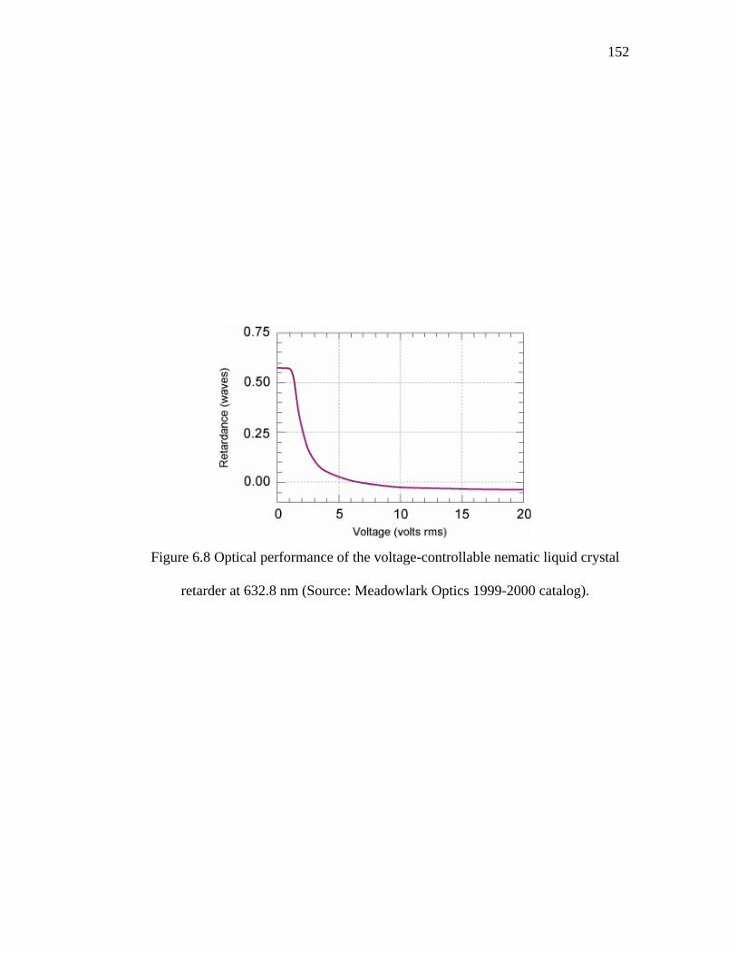
152
Figure 6.8 Optical performance of the voltage-controllable nematic liquid crystal
retarder at 632.8 nm (Source: Meadowlark Optics 1999-2000 catalog).
153
region with a size of 100 × 100 pixels at the center of image is displayed in Figure 6.9
and used for image processing. As can be seen from Figure 6.9, the mechanical rotation
of the analyzer contributes to the nonuniform intensity distribution at different rotation
angles. Thus the performance of the rotating analyzer method could be limited by the
optical quality of the analyzer and the compensation of this effect might be required.
Before moving to image processing to calculate the birefringence vector ),( θφ , the
defect pattern caused by scratches or dust on the surfaces of the optical components and
the spatial noise are removed to some extent by the image filtering as shown in Figure
6.10.
Figure 6.11 and Figure 6.12 show the 2-D distributions of the retardation θ and the fast
axis angle φ of the principal birefringence axis (i.e., the fast axis) in the voltage-
controllable nematic liquid crystal retarder for different voltage. For a convenient
visualization of fast axis angle, each neighboring 5 × 5 pixels is averaged and
corresponds to one arrow in the 2-D profile of φ . Here note that the long axis of the
liquid crystal molecules is defined as the slow axis, which is characterized by the
extraordinary index. With no voltage presenting, the molecules lie parallel to the surfaces
of the nematic liquid crystal plate and the maximum retardation is obtained. As the
voltage applied across the liquid crystal layer increases, the molecules become reoriented
such that the slow axis moves to be parallel to the applied electric field. Thus the
effective birefringence decreases and it causes a reduction in the retardation θ with the
increased applied voltage as shown in Figure 6.10(b) and 6.11(b). From the chart in
Figure 6.8, the retardations are around 14° and 7° for voltage 3.23V, 3.99V respectively.
The calculated results are in good agreement with these values after considering the
154
deviation. The deviation is decreased with higher voltage. This is corresponding to the
liquid crystal molecules arranging more uniformly. However, the direction of the fast
axis θ that is originally aligned parallel to the windows of the liquid crystal plate does not
change, independent of the applied voltage as shown in Figure 6.10(a) and 6.11(a). The
2-D distribution of the birefringence vector ),( θφ in the testing liquid crystal is quite
uniform, and the signal-to-noise ratio (SNR) decreases when the induced effective
retardation comes close to 0° by increasing the applied voltage.
6.2.3 Conclusion
The test experiment verified the effectiveness of the rotation analyzer method for
a single domain, and so for odd number of stacked domains. While applying this method
to even number of stacked domains, Jones matrix ),( θφRJ in equation (6.24) should be
given by equation (6.16). While, the output intensity is:
( )[ ]θφ sin2sin12
22 +Φ−=+= oyx
IEEI (6.28)
For this case, the retardation can be calculated the same way as one domain, but the fast
axis angle will change sign. For a real measurement, this method alone cannot determine
the sign of the fast axis angle in a single measurement configuration. However, the
retardation is reliable. Then the total thickness of these two direction 90° domains can be
concluded since the total thickness is fixed and measurable. The growth of these two
direction 90° domains can be also measured under external bias condition, such as
electric field, stress, and change of temperature. To identify the orientation of the domain,
it is only necessary to know the change of the fast axis angle but the exact distribution of
it. Sudden changing the sign of the fast axis angle will not happen if all the reorientation
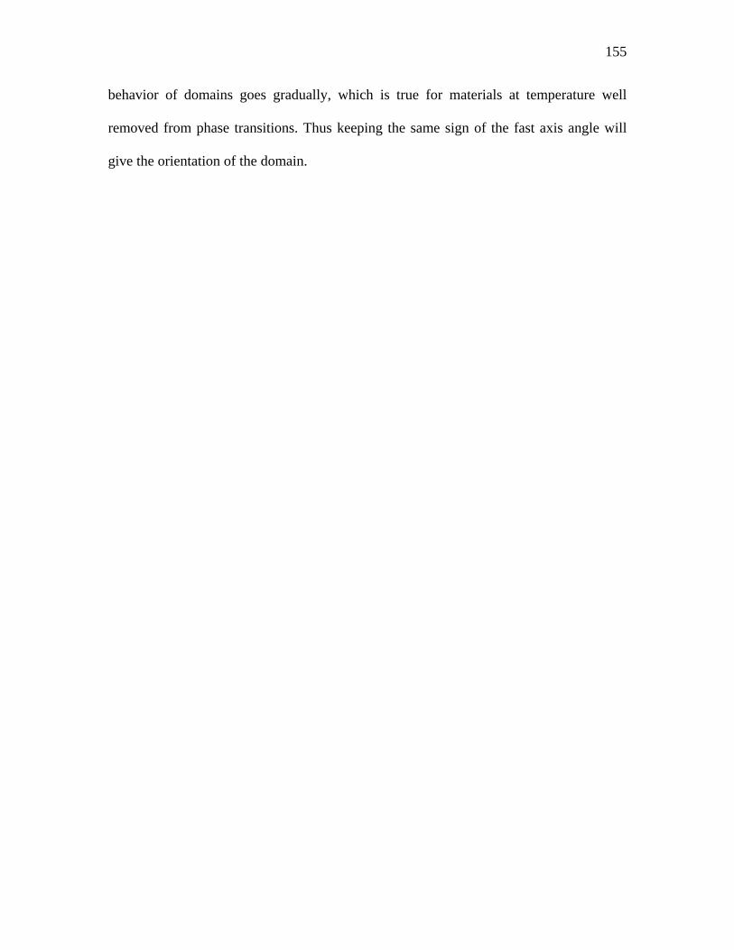
155
behavior of domains goes gradually, which is true for materials at temperature well
removed from phase transitions. Thus keeping the same sign of the fast axis angle will
give the orientation of the domain.
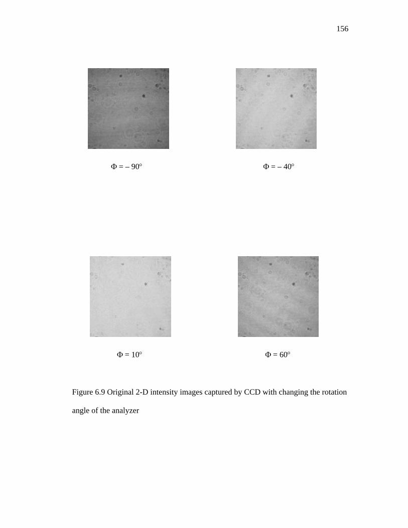
156
Φ = – 90° Φ = – 40°
Φ = 10° Φ = 60°
Figure 6.9 Original 2-D intensity images captured by CCD with changing the rotation
angle of the analyzer
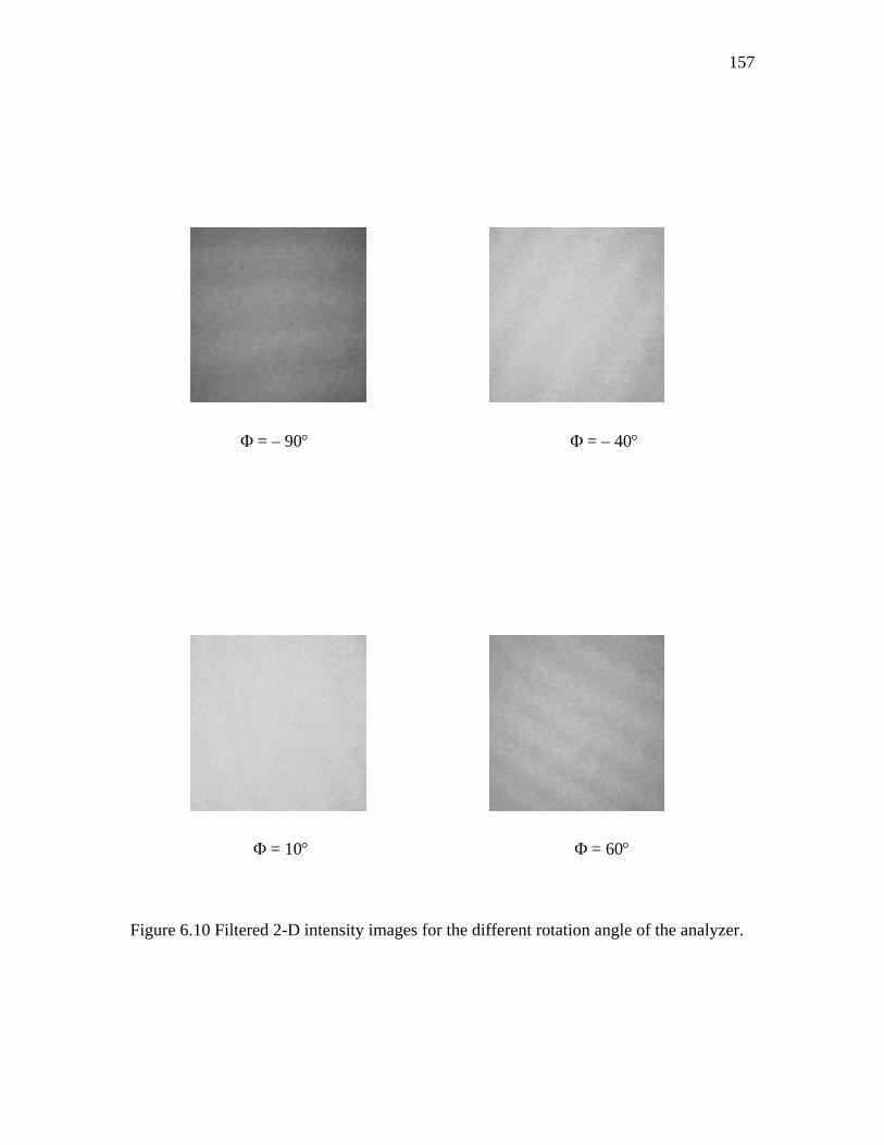
157
Φ = – 90° Φ = – 40°
Φ = 10° Φ = 60°
Figure 6.10 Filtered 2-D intensity images for the different rotation angle of the analyzer.

158
1 25 50 75 1001
25
50
75
100
(a) 2-D profile of fast angel φ, average: 48.61 deg., standard deviation: 5.06 deg.
1 25 50 75 100
1
25
50
75
100
(b) 2-D profile of the retardation θ, average: 12.5 deg., standard deviation: 1.866 deg.
Figure 6.11 2-D profile of birefringence ),( θφ with applied voltage 3.23V
φ
Fast axis
0o
5o
10o
15o
20o
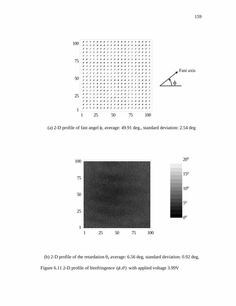
159
1 25 50 75 1001
25
50
75
100
(a) 2-D profile of fast angel φ, average: 49.91 deg., standard deviation: 2.54 deg
1 25 50 75 100
1
25
50
75
100
(b) 2-D profile of the retardation θ, average: 6.56 deg, standard deviation: 0.92 deg,
Figure 6.11 2-D profile of birefringence ),( θφ with applied voltage 3.99V
φ
Fast axis
0o
5o
10o
15o
20o
160
Chapter 7
Discussion and Conclusion
7.1 Discussion and conclusion
7.1.1 Local Polarization and Burns Temperature
As a peculiarity of relaxor ferroelectrics, the Burns temperature so far has not
been well understood. The Burns temperature was first discovered by Burns and Dacol
[Burns and Dacol, 1983a, b] in the ferroelectric systems of PLZT, PMN, and PZN by
optical refractive index measuement. Later it was found the existence of the burns
temperature in more ferroelectrics system of PTiSn, KSR [Burs and Dacol, 1990a], BSN
[Bhalla et. al, 1987], and BSKNN [Bhalla et. al, 1992]. Now it is believed that the Burns
temperature, marking the appearance of significant deviation of refractive index or
birefringence from quasilinear temperature dependence, is one of the intrinsic characters
of the relaxor ferroelectrics with diffuse phase transition. So far the determination of the
Burns temperature is by means of the optical method measuring either the refractive
index or birefringence, while it can be supported by other method such as neutron
scattering spectrum [Gerhring et. al. 2001] and Raman spectrum [Svitelskiy et. al., 2005].
Burns and Dacol connected this deviation with the onset of the formation of polar
nanoregions, caused local polarization consequently. The breakdown of translation
symmetry resulting from the heterogeneous ions on crystallographic sites leads variation
of Curie temperature for nanoregions which undergo transition to a lower symmetry polar
state before others. It is notable that the local polarization dP derived from refractive
index or birefringence is not from any detailed microscope model but general symmetry
consideration. 3nΔ or 231 Pn ∝Δ come from the fact the high temperature phase can be
161
treated as centrosymmetric and any polarization (local or macroscopic) can be treated as
an expansion at P=0. Thus the first term will be 2P term. It also should be reminded that
the derived local polarization dP is really the mean square root −
2dP . This keeps the
answer of the question whether the observed polarization is static or dynamic unknown
while the average polarization is zero. In general, one would expect that dynamical
inversion of dP in nano polar region would be modulated by a weak external 3E field so
as to change the fraction of up and down polarizations and thus contribute a significant
component to the dielectric polarizability. In the static model the dipolar component
which appears at temperature well above is already frozen. Polarizability would now be
contributed by expansion and contraction of the polar region and the dielectric maxima
would be essentially due to cooperative ordering.
Vakhrushev and Shapior [Vakhrushev and Shapior, 2002] have directly observed
a soft ferroelectric mode associated with the Curie-Weiss behavior of the dielectric
constant by inelastic neutron scattering measurements of PMN. The frequency of the soft
mode exhibits a minimum near the Burns temperature. This confirmed that at the Burns
temperature a local phase transition occurs resulting in a crossover of the critical
dynamics. Above Td the dynamics is of displacive type, while below it is governed by a
relaxation of the large polar regions.
More recently Toulouse et. al.[ Toulouse, et. al., 2005, Svitelskiy, et. al., 2005]
proposed that the Burns temperature (in order to avoid confusion the Burns temperature
denoted as TB hereafter) is not the temperature when polar nanoregion appear, but the
temperature at which the life time of the dynamic correlations between the off-center Pb
ions exceeds the period of the TO phonon, then appearing static on the time scale of the
162
phonon ( or quasidynamic on the absolute time scale) after their investigation on the
Raman spectrum of PZN. This crossover from fully dynamic to quasidynamic is marked
by a narrowing down of the low frequency features of the Raman spectrum, the
disappearance of the long wavelength TO phonon from the inelastic neutron scattering
spectrum as well as a faster-than-linear decrease with temperature of the refractive index.
It's also the temperature at which the growing lifetime of the dynamic correlations
between off-center ions exceeds the inverse frequency of the TO phonon. Above TB, the
local intersite motion of the off-center ions is fast and uncorrelated, dynamically
broadening the TO phonon. Below TB, these correlations, though still dynamic in the
absolute (absence of local strain fields), will appear static to the TO phonon whose
frequency will then increase. The permanent polar nanoregions appear at so-called
'intermediate temperature' Td, which is between the Burns temperature TB and freezing
temperature Tf. At Td local phase transitions begin to take place. Because these are local,
they generate local strain field. Thus Td marks the onset of local phase transition, or the
appearance of static or permanent correlations of the off-center ion displacements as well
as the off-centering of other previously on-center ions. The temperature range between Td
and Tf is dominated by the rotation of the polar nanoregions and can appropriately be
designated as a quasistatic stage. The freezing temperature Tf is marked by a drastic
overall drop in scattered intensity and abruptly changes in the Raman spectrum, which
strongly suggest an arrest of the low frequency relaxational motion. It is also the
temperature at which the frequency dependence disappears in the dielectric constant and
an underdamped TO phonon reappears in the neutron scattering spectrum. Below Tf, the
163
dynamic appears to be dominated by renormalized TA-TO coupling induced by static
disorder.
Whether the Burns temperature marks the appearance of the polar nanoregion is
critical for the optical measurement of PBN57. If it's true, then both the measurement of
refractive index and birefringence should yield the same Burns temperature for each
wavelength. However, even if this is true, the difference of the Burns temperature can
only ascribe to the measurement error. As mentioned in chapter 3 that the unstable high
temperature the refractive index could not yield the true Burns temperature, and
generating such error is possible.. If the above model is true, i.e. the Burns temperature
marks the crossover between the soft mode and order-disord dynamics. And the Burns
temperature for refractive index and birefringence are not necessary the same.
7.1.2 Optical Curie Region
In chapter 3 the optical Curie region is defined as the temperature region between
the deviation temperatuire TD and the Burns temperature Td. Both the coupling between
the light and the nano/micro polar regions and the dipole-dipole interaction between polar
regions resulted in the optical Curie region, which decreases with optical frequency. This
is shown in the Figure 8.1 with two aspects. The average size of polar regions at low
temperature is lager than that at high temperature since in relaxor ferroelectrics the
macrodomain transforms to microdomain with increasing temperature, i.e. the average
size of polar region decreases with temperature. On the other hand a certain frequency is
more sensitive to some polar regions with a corresponding sizes but almost invisible to
other polar regions with much different sizes if considering coupling between light waves
and polar regions. Thus there is a one-to-one map between any two of the three amounts:
164
the light frequency, the deviation temperature, and the size of polar regions. The large
frequency of light corresponds to small size polar regions while the latter prefer high
temperature.
The optical Curie region decreases with frequency. The deviation temperature TD
and the Burns temperature Td have the tendency that approaches to the Tm with a high
enough frequency, and the relaxor ferroelectric behaves maybe more like a normal
ferroelectric. The deviation temperature significantly marks the breakup of macroscopic
polar-regions approaching relaxor phase transition. It's reasonable to analogize the
deviation temperature to freezing temperature Tf since the freezing temperature marks the
ending of the diffuse phase transition. If the frequency is low enough that has no coupling
with polar regions at all, the deviation temperature maybe approach to freezing
temperature Tf. Thus one can speculate that the frequency dependent deviation
temperature has an upper bound, i.e. temperature of dielectric maxima, Tm, and a low
bound, freezing temperature Tf.
With the accurate determined deviation temperature it is possible to estimate the
average size of the polar regions at different temperature.
The isotropic temperature Ti has the same trend with frequency as dielectric
maximum temperature Ti. However this is not common phenomenon for relaxor
ferroelectric. This only occurs for the relaxor whose birefringence has different sign in
the high temperature paraelectric state and low temperature ferroelectric state. The
existence of isotropic temperature Ti is of great interest for application, such as optical
valve.
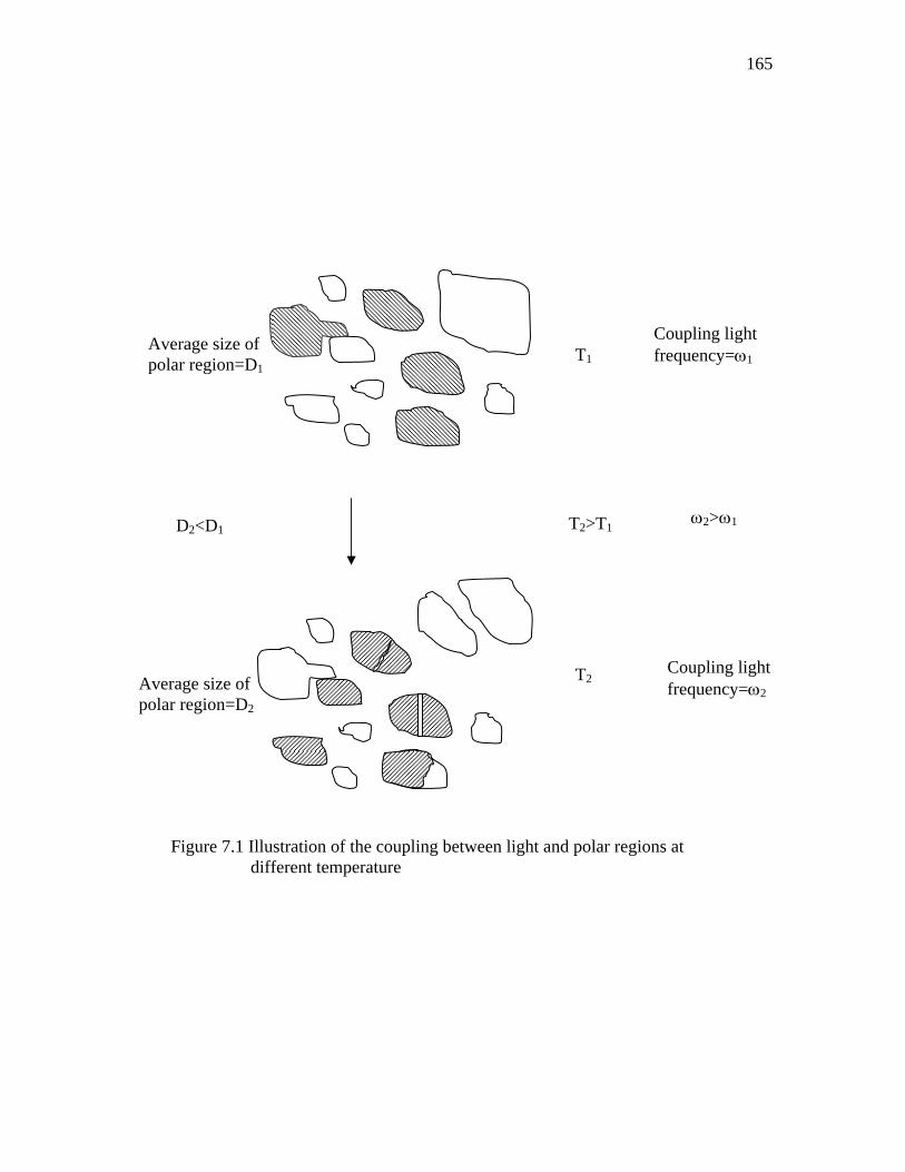
165
T1
T2
T2>T1
Figure 7.1 Illustration of the coupling between light and polar regions at different temperature
Average size of polar region=D1
Average size of polar region=D2
D2<D1
Coupling light frequency=ω1
Coupling light frequency=ω2
ω2>ω1
166
7.1.3 Dipole-Dipole interaction
It was turned out that the interaction between the polar regions in relaxor
ferroelectrics system could not be omit. First, the interaction between the polar regions
distinguishes the relaxor ferroelectrics from normal dielectrics whose optical refractive
index can be describe by the single oscillator model, resulting the existence of optical
Curie region. Second, thermo-optic coefficients in the low temperature ferroelectric state
have major contribution from polarization term. These two are the most direct proofs for
nonneglectable interaction between polar regions. The last one is coming from the results
of transmission spectrum of PZN-0.12PT. The derived energy of the phonon is two large
to be considered as phonon energy but rather the orbit-spin interaction or the interband
transition. The interaction between the polar regions could make the energy band splitting
very complicate and make the interband transition possible. Recently more and more
theories model based on random field can give some explain for experiment. Taking into
account the interaction between polar regions is the essential part of random field.
7.2 Major results and conclusions
1)Temperature dependent birefringence and optical refractive indices of PBN
(Pb1-xBaxNb2O6) crystal (1-x=0.57) were measured in several optical wavelengths (λ=
694nm, 633nm, 535nm, and 450nm) to understand the optical frequency dependency of
ferroelectric phase transitions in relaxor ferroelectric crystals of tungsten bronze
structure. Local polarization is verified to be dynamically activated by thermal process
and probed effectively by suitable wavelength of light. An optical isotropic point, as
167
function of temperature and light frequency, is reported at which the crystal’s standing
birefringence is fully compensated by polarization.
2) A modified single oscillator model is used to calculate the index of refraction
in the ferroelectric phase. The deviation temperature from the single oscillator model is
reported to be significant marking the crossover from macroscopic to microscopic
polarization. A new parameter, optical Curie temperature region, defined by the
temperature difference between the well known Burns temperature and the deviation
temperature (from the single oscillator model for index of refraction) is explored for its
significance in depolarization behavior of the micro- to nano-polar regions of the
ferroelectric relaxor.
3)Temperature dependent optical index of refraction of PZN-0.12PT (1-
x)PbZn1/3Nb2/3O3-xPbTiO3, x=0.12, were also studied with emphasis on poling effect.
The refractive index n3 decreases as a result of [001] poling. Temperature dependent
effective energy of dispersion oscillator 0E and dispersion energy dE were calculated
using single oscillator model and found that 0E and dE increased by 32% and 60% after
[001] poling, respectively. Birefringence of poled PZN-0.12PT also was measured with
several frequency and varying temperature. The polarization derived from refractive
index and birefringence were consistent with each other. The remnant polarization was
increased by approximately 30% as a result of [001] poling.
4) Transmission spectrum of PZN-0.12PT was measured from near UV to IR for
both poled sample and unpoled sample. Transmission was improved significantly after
poling. By analyzing the transmission spectrum in the visible range, optical band gap and
168
lattice phonon were determined. The existence of hydrogen in PZN-0.12PT single crystal
grown by flux method was postulated based on evidence obtained by FTIR.
5) For accurate and fast birefringence measurement, which is of fundamental
important to device design, quality control, and various sensing functions, a two-
dimensional birefringence profiling and analysis system was designed and implemented
successfully. Jones matrices of two and three 90° domains are derived and conclude that
odd number of stacked 90° domains can be treated as a single 90° domain while even
number of stacked 90° domains can be treated as two 90° domains. By rotating analyzer
method a test experiment using voltage controllable liquid crystal as sample is
demonstrated.
-
7.3 Suggestion for future work
An extension of the present study can be made into areas related this work but not
explore. The following are but a few suggestions for the future work.
1) Apply the whole procedure, including the measurement of optical refractive
index and birefringence and data modeling, to other relaxor ferroelectric composition.
Check if the freezing temperature Tf is the limitation of the frequency dependent
deviation temperature TD.
2) Continue to verify the optical Curie region with higher frequency, Combine
with other measurement methods, such as SEM, to explore to relation of light wavelength
with the size of polar regions
3) Temperature dependent transmission would be interesting to explore how the
optical bandgap changes with temperature.
169
4) Temperature dependent IR spectroscopy to explore the TO phonon.
5) Using the 2D index mapping system to study the domain under varying
temperature and other conditions.
170
References:
Abe S., Fujishima T., Tsubone T., Fujimura R., Ono H., Matoba O., Oda K., Shimura T.,
and Kuroda K., Opt.Lett. Vol.28, No. 6 ,440(2003)
Abedin K. S., Ito H., J. Appl. Phys. 80, 6561 (1996)
Arabidze A. A. and Chikvaidze B. Ya., Sov. Phys. Solid State, 21(4), 722(1979)
Barad Y., Lu Y.,. Cheng Z. Y, Park S.-E., and Zhang Q. M., Appl. Phys. Lett. 77, 1247
(2000).
Beudon D., Boudjema E. H., Bihan R.L., Jpn. J. Appl. Phys. Supplement, 24 (2), 545
(1985)
Bhalla A. S., Guo R., Cross L. E., Burns Gerald, Dacol F. H., and Ratnakar R.
Neurgaonkar, Phys. Rev. B 36, 2030 (1987)
Bhalla A.S., Guo R., and Cross L.E., Burns Gerald, Dacol F. H., and Ratnakar R.
Neurgaonkar, J. Appl. Phys. 71, 11 (1992)
Blinc R., Dolinsek J., Gregorovic A., Zalar B., Filipic C., Kutnjak Z., Levstik A., and
Pirc R., Phys. Rev. Lett. 83, 424 (1999)
Blinc R., Gregorovi A., Zalar B., Pirc R., and Lushnikov S. G., Phys. Rev. B 61, 253
(2000).
Bobnar V., Kutnjak Z., Pirc R., Blinc R., and Levstik A., Phys. Rev. Lett. 84, 5892 (2000)
Brebner J. L., Jnadl S., Lepine Y., Phys. Rev. B23, 3816(1981)
Burns G. and Dacol F. H., Solid State Commun., 48, 853 (1983a)
Burns G. and Dacol F. H., Phys. Rev. B., 28, 2527 (1983b)
Burns G. and Dacol F. H., Phys. Rev. B., 30, 4012 (1984)
Burns G., Phase transitions, 5, 261 (1985)
171
Burns G. and Dacol F. H., Solid State Commun., 58, 567 (1986)
Burns G. and Dacol F. H., Ferroelectrics, 104, 25 (1990a)
Burns G., Dacol F. H., Neurgaonkar R. R., Bhalla A. S. and Guo R., Ferroelectrics, 108,
189 (1990b)
Burns G., Dacol F. H., Neurgaonkar R. R., Bhalla A. S. and Guo R., Appl. Phys. Lett.
57(6), 543 (1990c)
Chattopanhuay S., Ayyub P., Palkar V. R., and Multani M., Phys. Rev. B 52, 13177
(1995).
Cheng Z. Y., Cheng, L. Y., and Yao X., J. Appl. Phys. 79, 8615(1996)
Choi S. W., Shrout T. R., Jang S. J., Bhalla A. S., Ferroelecrics, 100, 29 (1989)
Cohen R. E. and Krakuer H., Ferroelecrics 111, 57 (1990)
Cohen R.E., J. Phys. Chem. Solids, 61, 139(1999)
Cross L. E., Ferroelectrics 76, 241 (1987);
Cross L. E., Ferroelectrics 151, 305 (1994).
DiDomenico Jr. M. and Wemple S. H., Phys. Rev.166, 565(1968)
DiDomenico Jr. M. and Wemple S. H., J. Appl. Phys. 40, 720 (1969a)
DiDomenico Jr. M. and Wemple S. H., J. Appl. Phys. 40, 735 (1969b)
Dierolf V., Sandmann C., Kim S., Gopalan V., and Polgar K., Appl. Phys. 93, 2295
(2003)
Dow J. D., and Redfield D., Phys. Rev. B. 5, 594(1972)
El-Fadl A. Abu,. Gaffar M. A, Omar M. H., Physica B 269, 403(1998)
Fu Desheng, Suzuki K., Kato K., and Suzuki H., Appl. Phys. Lett. 82, 2130 (2003)
Fu H. X., Cohen R. E., Nature 403, 281(2000)
172
Garcia A. and Vanderbilt D., Appl. Phy. Lett. 72, 1981(1998)
Gerhring, P. M., Wakimoto S., Ye Z. G., and Shirane G., Phys. Rev. Lett. 87, 277601
(2001)
Ghosez Ph. and Rabe K. M., Appl. Phys. Lett. 76, 2767 (2000).
Ghosh G., Opt. Lett. 19, 1391 (1994)
Ghosh G., J. Appl. Phys. 78, 6752(1995)
Glass A. M., J. Appl. Phys. 40, 4699 (1969).
Glinchuk M. D., Eliseev E. A., Stephanovich V. A., Hilczer B., Phys. of the Solid State,
43, 1247 (2001)
Gopalan V., Mitchell T., Furukawa Y., and Kitamura K., Appl. Phys. Lett. 72, 1981
(1998).
Gruverman A., Auciello O., and Tokumoto H., Annu. Rev. Mater. Sci. 28, 101 (1998).
Guo R., Bhalla A. S., Randall C. A., Chang Z. P., and Cross L. E., Ferroelectrics, 93, 989
(1989)
Guo R., Bhalla A. S., and Cross L. E., Appl. Optics, 29, 904 (1990)
Guo R., Bhalla A. S., Randall C. A., and Cross L. E., J. Appl. Phys., 67(10), 6405 (1990)
Guo R., Bhalla A. S., Randall C. A., Chang Z. P., and Cross L. E., J. Appl. Phys. 67,
1453 (1990)
Guo R., , Evans Jr. H.T., Bhalla A.S., ISAF '96. Proceedings of the TenthIEEE
International Symposium on Applications of Ferroelectrics, 1, 241 (1996)
Haefke H., Luithi R., Mayer K. P., and Guntherodt H. J., Ferroelectric, 151, 143 (1994)
Hasiang H. I. and Yen S. F., J. Am. Ceram. Soc. 79, 1053 (1996)
Herrington J. R., Discher B., Rauber A., and Schneider J., Solid state Commun. 12,
351(1973)
173
Hidaka T., Maruyama T., Saitoh M., Mikoshiba N., Shimizu M., Shiosaki T., Wills L. A.,
Hiskes R., Dicarolis S. A., and Amano Jun, Appl. Phys. Lett. 68, 2358 (1996)
Hilczer B., Szezesniak L., Mayer K. P., Ferroelectric, 97,59 (1989)
Houde D., Lepine Y., Pepin C., Jandl S., and brebner J. L., Phys. Rev. B 35, 4948(1987)
Hunsche S., Grone A., Greten G., Kapphan S., Pankrth R., and Seglins J., Phys. Status
Solidi A 148,629 (1995)
Isupov V. A., Ferroelectrics 90, 113 (1989)
Isupov V. A., Phys. Satatus Solidi B213, 211 (1999)
Isupov V. A., Phys. Solid State 45, 1107 (2003)
Ivanov N. R. Volk T. R., Ivleva L. I., Chumakova S. P., and Ginzberg A. V.,
Crystallography Reports, 47(6), 1023 (2002)
Iwata M., Araki T., Maeda M., Suzuki I., Ohwa H., Yasuda N., Orihara H., and Ishibashi
Y., Jpn. J. Appl. Phys., Part 1 41, 7003 (2002)
Izawa Y., and Nakai S., Applied optics, 33,6368 (1994)
Jaffe B., Cook Jr. W. R., and Jaffe H., "Piezoelectric Ceramics", Academic Press,
London, (1971)
Kapphan S., and Weber G., ferroelectrics 37, 637 (1981)
Kinase W., Ohnishi N., Yoshikawa M., and Mori K., Ferroelectrics, 56, 165 (1984)
King-Smith R. D. and Vanderbilt D., Phys. Rev. B 49, 5828(1994)
Kirilov V. V. and Isupov V. A. Ferroelectrics 5, 3 (1973)
Kleemann W. J. Non-Crystalline Solids, 307-310, 66 (2002)
Kliger D. S., Lewis J. W., and Randall C. E., "Polarized light in optica and spectroscopy",
Academic Press, Inc., (1990).
Koray E.Akdogan and Safari Ahmad, Jpn. J. Appl. Phys., Part 1 41, 7170 (2002)
174
Kuwata J., Uchino K., and, Nomura S., Ferroelectrics, 22, 863 (1979)
Kuwata J., Uchino K., Nomura S., Jpn. J. Appl. Phys. 21, 1298(1982)
La-Orauttapong D., Toulouse J., Robentson J. L., Ye Z.-G., Phys. Rev. B 64,
212101(2001)
La-Orauttapong D., Noheda B., Ye Z.-G., Gehring P. M., Toulouse J., Cox D.E., and
Shirane G., Phys. Rev. B. 65, 144101(2002)
Laulicht L. and Benguigui L., Solid state Commun. 32, 771(1979)
Lee M., Feigelson R. S., Liu A., Hesselink L., Route R. K., Phys. Rev. B, 56, 7898(1997)
Lim L.C., Rajan K.K, J.Crystal Growth 271, 435(2004)
Lines, M. E., Glass A.M., "Principles and Applications of Ferroelectrics and Related
Materials", Oxford University Press, (1977)
Liu A.Y., Bashaw M.C., and Hesselink L., Lee M., Feigelson R.S., Opt. Lett.
22,187(1997)
Lu Y., Cheng Z.-Y., Park S.-E., Liu S.-F., and Zhang Q., Jpn. J. Appl. Phys. 39, 141
(2000).
Lu Y., Cheng Z.-Y., Barad Y., and Zhang Q. M., J. Appl.Phys. 89, 5075 (2001).
Lu C. J., Ren S. B., Shen H. M., Liu J. S., and Wang N. Y., J. Phys.: Condens. Matter 8,
8011 (1996).
Martirena H. T. and Burfoot J. C., Ferroelectric 7, 151 (1974)
Mathan N. de, Husson E., Calvarin G., Gavarri J. R., Hewat A. W., and Morell A., J.
Phys.: Condens. Matter 3, 8159 (1991).
McHenry D. A., Giniewicz J., Jang S. J., Bhalla A. S., Shrout T. R., Ferroelectrics, 93,
1137 (1989)
175
McHenry D. A., Ph. D. Thesis, The Pennsylvania State University , May(1992)
Mulvihill M. L., Cross L. E. and Uchino K., J. Am. Ceram. Soc. 78, 3345 (1995)
Narasimhamurty, T. S. "Photoelastic and Electro-optic properties of crystals", Plenum
Press, New York, (1981)
Newnham R. E., "Structure - Property Relations", Springer Verlag, New York, (1975).
Nishida Y. and Yamanaka M., Review of Sci. Instru. 72, 2387 (2001)
Noheda B., Cox D. E., Shirane G., Gonzalo J., Cross L. E., and S. Park, Appl. Phys. Lett.
74, 2059(1999)
Noheda B., Cox D. E., Shirane G., Gonzalo J., Park S., Cross L. E., and Zhong Z., Phys.
Rev. Lett. 86, 3891(2001)
Nye J. F., "Physical Properties of Crystals" (Clarendon Press, Oxford, 1990)
Ohmi M., Akatsuka M., Ishikawa K., Naito K., Yonezawa Y., Nishida Y., Yamanka M.,
Paz de Araujo C. A., Cuchiaro J.D., McMillan L. D., Scott M. C., and Scott J. F., Nature,
374, 627 (1995)
Phillips J. C., Phys. Rev. Lett. 20, 505 (1968).
Phillips J. C. and Van Vechten J. A., Phys. Rev. Lett. 22, 705 (1969).
Pirc R. and Blinc R., Phys. Rev. B 60, 13470 (1999).
Pirc R. and Blinc R., Phys. Rev. B 61, 14 448 (2000).
Pirc R., Blinc R., and Bobnar V., Phys. Rev. B 63, 054203 (2001)
Rabe K. M. and Cockayne E., First-priciples calculations for ferroelectric, Fifth
Williamsburg Workshop AIP, 61 (1998)
Randall, C. A. Bhalla A. S., Jap. J. Appl. Phys. 29 327(1990a)
Randall C. A., Bhalla A .S., Shout T. R., and Cross L. E., J. Mater. Res. 5, 829(1990b)
176
Randall C. A., Guo R., Bhalla A. S., and Cross L. E., J. Mat. Res., 6(8), 1720 (1991)
Santos Ivair A., Garcia D., Eiras José A., and Arantes Vera L., J. Appl. Phys. 93, 1701
(2003)
Schlag S. and Eicke H. F., Solid State Commun. 91, 883 (1994).
Schlarb U. and Betzer K., Physics Rev. B48, 15614 (1993)
Scott J. F., Duiker H. M., Beale P. D., Pouligny B., Dimmler K., Parris M., Butler D., and
Eaton S., Physica B & C 150, 160 (1988).
Setter N. and Cross L. E. J. Appl. Phys. 51(8), 4356 (1980)
Shrout T. R., Fielding, Jr. J., Ultrasonics Symposium, 1990. Proceedings., IEEE 1990 , 4-
7 Dec. 2, 711(1990)
Shrout T. R., Halliyal A., Am. Ceram. Soc. Bulletin, Vol. 66, No.4, 704(1987)
Skettrup G. A. T., Phys. Rev. B. 18, 2622(1978)
Smolenskii and Isupov V. A., Dokl. Akad. Nauk SSSR 9,653 (1954).
Smolenskii G. A., J. Phys. Soc. Japan 28, Suppl. 26(1970)
Svitelskiy O., La-Orauttapong D., Toulouse J., Chen W., Ye Z.-G, Phys. Rev. B. 72,
172106(2005)
Tangantsev A. K., Phys. Rev. Lett, 72,1100(1994)
Toulouse J., Jiang F., Svitelskiy O., Chen W., Ye Z.-G, Phys. Rev. B. 72, 184106(2005)
Tsay Y. F., Bendow B., and Mitra S. S., Phys. Rev. B8, 2688 (1973)
Tsay Y. F., Lipson H. G., and Ligor P. A., J. Appl. Phys. 48,1953(1977)
Tuttle B., Headley T., Drewien C., Michael J., Voigt J., and Gavino T., Ferroelectrics
221, 209 (1999).
Tybell T., Ahn C. H., and Triscone J.-M., Appl. Phys. Lett. 75, 856 (1999)
177
Uchino K. and Nomura S., Ferroelectr. Lett. Sect. 44, 55 (1982)
Uchino K., cer. Bull. 65, No. 8, 647 (1986)
Uchino K, "Ferroelectric Devices", Marcel Dekker Inc., New York, (2000)
Varshni Y. P., Physica 34, 149 (1967)
Vakhrushev S. B., and Shapior S. M., Phys. Rev. B 66, 214101 (2002)
Viehland D., Jang S. J., Cross L. E., and Wuttig M., J. Appl. Phys. 68, 847 (1990a).
Viehland D., Jang S. J., Cross L. E., J. Appl. Phys. 68, 2916 (1990b).
Viehland D., Li J. F., Jang S. J., Cross L. E., Phys. Rev. B 43, 8316 (1991)
Vugmeister B. E. and Rabitz H., Phys. Rev. B 57, 7581 (1998)
Wan X., Xu H., He T., Lin. D., and Luo H., J. Appl. Phys, 93, 4766 (2003)
Wan X., Luo H., Wang J., Chan H., and Choy C. Solid state Commun., 129, 401 (2004)
Wemple S. H. and DiDomenico Jr. M., Phys. Rev. Lett. 23, 1156 (1969)
Wemple S. H. and DiDomenico Jr. M., Phys. Rev. B 3, 1338 (1971)
Wemple, S. H., "Laser handbook", eds Arecchi F. T. and Schulz-DuBois E. O. 975
(1972)
Wemple S. H., Phys. Rev. B 7, 3767 (1973)
Wemple S. H., J. Chem, Phys. 67, 2151 (1977)
Weyrich K. H. and Madench R.P., Ferroelecrics 111, 9 (1990)
Whatmore R. W., Osbond P. C., and Shorrocks N. M., Ferroelectrics, 76, 351 (1987)
Wu Z., Cohen R. E., and Singh D. J, "Fundamental physics of ferroelectric" 2003 edited
by David P.K. and Singh D. J., (2003)
Xiao Xiaoyue, Xu Yan, Zeng Zhigang, Gui Zhilun, Li Longtu, and Zhang Xiaowen, J.
Mater. Res. 11, 2302 (1996)
178
Xu Y., "Ferroelectric Materials and their Applications" North Holland, Amsterdam,
(1991)
Yamashita Y., Am. Ceram,Soc,Bull,73, 74(1994)
Yang T. J., Mohideen U., and Gopalan V., Phys. Rev. Lett. 82, 4106 (1999)
Yang X., Lowell T. Wood, Miller, Jr. John H., and Strikovski M., J. Appl. Phys. 92, 1168
(2002)
Yao X., Chen Z., and Cross L. E., J. Appl. Phys, 54, 3399 (1984)
Zhang S. J. unpublished data
Zhong W., Jiang B., Zhang P., Ma J., Chen H., Yang Z., and Li L., J. Phys.: Condens.
Matter 5, 2619 (1993).
Zhong W. L., Wang Y. G., Zhang P. L., Phys. Rev. B 50, 698 (1994).
Zhong W. L., Wang Y. X., Wang C. L., Jiang B., and Bursill L. A., Ferroelectrics 252,
11 (2001).
Zhu S., Chen Y., and Fang J., Phys. Rev. B. 35, 2980(1987)
Zook J. D. and Casselman, T. N., Phys. Rev. Lett. 17, 960 (1966)
Zysset B., Biaggio I., and Gu ter P., J. Opt. Soc. Am. B 9, 380 (1992)
179
VITA
Chunlai Li was born on April 29, 1976 in Xiaogan city, Hubei, China. In high
school he excelled in national math competition and was exempted from the entrance
exam for college. He majored in physics in Wuhan University from 1992-1996. In 1999
He received his master degree in atomic and molecular physics from Wuhan Institute of
Physics and Mathematics, the Chinese Academy of Sciences. He studied in the
department of electrical engineering, the Pennsylvania Sate University since 2000 fall.