Dispersion and Tretament Perfomance Analysis of an UASB Reactor Under Different Hydraulic Loading Rates

8/18/2019 Dispersion and Tretament Perfomance Analysis of an UASB Reactor Under Different Hydraulic Loading Rates

http://slidepdf.com/reader/full/dispersion-and-tretament-perfomance-analysis-of-an-uasb-reactor-under-different 1/8

Available at www.sciencedirect.com

jo ur na l ho me pa ge : ww w. el sevier .com /l oc at e/ wa tr es

Dispersion and treatment performance analysis of an UASB

reactor under different hydraulic loading rates

M.R. Penaa,, D.D. Marab, G.P. Avellaa

aInstituto Cinara, Universidad del Valle, A.A 25157, Cali, Valle del Cauca, ColombiabSchool of Civil Engineering, University of Leeds, Leeds LS2 9JT, UK

a r t i c l e i n f o

Article history:

Received 15 October 2003

Received in revised form

1 November 2005

Accepted 8 November 2005

Available online 6 January 2006

Keywords:

Dispersion

Domestic wastewater

Flow pattern

Hydrodynamics

Mixing

Segregation

UASB

A B S T R A C T

Mixing and transport phenomena affect the efficiency of all bioreactor configurations. An

even mixing pattern at the macro-level is desirable to provide good conditions for substrate

transport to, and from, the microbial aggregates. The state of segregation of particulate

material in the reactor is also important. The production of biogas in anaerobic reactors is

another factor that affects mixing intensity and hence the interactions between the liquid,

solid and gaseous phases. The CSTR model with some degree of short-circuiting, dead

zones and bypassing flows seems to describe the overall hydrodynamics of UASBs.

However, few data are available in the literature for full-scale reactors that relate process

performance to mixing characteristics. Dispersion studies using LiCl were done for four

hydraulic loading rates on a full-scale UASB treating domestic wastewater in Ginebra, Valle

del Cauca, southwest Colombia. COD, TSS, and Settleable Solids were used to evaluate the

performance of organic matter removal. The UASB showed a complete mixing pattern for

hydraulic loading rates close to the design value (i.e. Q ¼ 10–13ls1 and HRT ¼ 8–6 h). Gross

mixing distortions and localised stagnant zones, short-circuiting and bypass flows were

found in the sludge bed and blanket zones for both extreme conditions (underloading and

overloading). The liquid volume contained below the gas–liquid–solid separator was found

to contribute to the overall stagnant volume, particularly when the reactor was

underloaded. The removal of organic matter showed a log-linear correlation with the

dispersion number.

& 2005 Elsevier Ltd. All rights reserved.

1. Introduction

The rate of conversion or removal of organic matter in any

bioreactor is governed by two main interrelated factors: the

performance of the microbiological processes and the hydro-

dynamics of the reactor. In biological wastewater treatment

there will always be more than one phase working at the

same time. The liquid, solid and gaseous phases interact with

each other during the normal operation of both aerobic and

anaerobic bioreactors, and therefore, different factors such as

mixing intensity, temporal and spatial variations of mixing,

degree of material segregation, gas bubbling pattern and

intensity, all affect the hydrodynamic behaviour of three-phase reactors (Bailey and Ollis, 1986; Levenspiel, 1999; Ottino

and Khakhar, 2000).

Previous studies on the hydrodynamics of three-phase

reactors such as UASBs have shown that they are best

described by the CSTR model with some short-circuiting,

dead zones and bypass flows (Ottino, 1990; Heertjes and

Kuijvenhoven, 1982). The hydrodynamic behaviour of UASBs

is also related to the type of influent-feeding device, upflow

velocity, sludge bed depth and sludge blanket height, as well

ARTICLE IN PRESS

0043-1354/$ - see front matter &

2005 Elsevier Ltd. All rights reserved.doi:10.1016/j.watres.2005.11.021

Corresponding author. Tel.: +57 2 3392345; fax: +57 2 3393289.E-mail address: [email protected] (M.R. Pen ˜ a).

W A T E R R E S E A R C H 4 0 ( 2 0 0 6 ) 4 4 5 – 4 5 2



as the biogas production rate (Heertjes and Kuijvenhoven,

1982; Bolle et al., 1986; Heertjes and van der Meer, 1978).

Heertjes and van der Meer (1978) assumed that the fluid

flow in the settling compartments of an UASB followed a

laminar regime, and that the sludge bed and sludge blanket

were completely mixed, although the sludge bed volume

could also have dead spaces, bypassing and returning flows.

They used the F-curve (step-response curve) to analyse the

mixing characteristics of the reactor, and this approach was

also adopted by subsequent workers (Heertjes and Kuijven-

hoven, 1982; Bolle et al., 1986; van der Meer and Heertjes,

1983). However, the use of the F-curve in some cases is not

very adequate to identify flow distortions within the reactor.

In this regard, Levenspiel (1999) points out that the F-curve

integrates effects within the system and it often yields a

smooth nice-fitting curve that may hide real flow distortions

within the reactor, especially in multiphase reactors. It has to

be also remembered that the F-curve is obtained from step

injection experiments as opposed to pulse injection tests (E-

curve). Moreover, the F-curve is obtained by integrating the

corresponding E-curve, and in this sense, F becomes a

cumulative function (Levenspiel, 1999).

The overall hydrodynamic behaviour of a multiphase

anaerobic reactor is the result of interactions between

several interdependent physical phenomena, such as fluid

flow properties, multiphase interactions, particle segre-

gation, chaotic advection and substrate dispersion, which

together determine the resultant mass transport pro-

cesses and hence the final performance of a given reactor.

This study was therefore, an evaluation of the overall

hydrodynamic behaviour of a full-scale UASB reactor trea-

ting tropical domestic wastewater at several hydraulic load-

ing rates. The analysis is focused on the macro-mixing

behaviour and process performance of the reactor; however,

liquid–sludge–gas interactions are also taken into account to

explain the results.

2. Materials and methods

2.1. Experimental unit

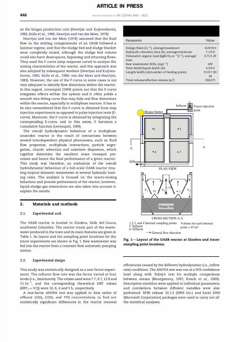
The UASB reactor is located in Ginebra, Valle del Cauca,

southwest Colombia. The reactor treats part of the waste-

water produced in the town and its main features are given in

Table 1. Its layout and the sampling point locations for the

tracer experiments are shown in Fig. 1. Raw wastewater was

fed into the reactor from a constant-flow automatic pumping

station.

2.2. Experimental design

This study was statistically designed as a one-factor experi-

ment. The influent flow rate was the factor varied at four

levels (i.e., treatments). The values used were 7.7, 9.7, 12.8 and

15.5s1, and the corresponding theoretical HRT values

(HRTt ¼ V /Q ) were 10, 8, 6 and 5 h, respectively.

A one-factor ANOVA test was applied to data series of

effluent CODt, CODf and TSS concentrations to find out

statistically significant differences in the reactor removal

efficiencies caused by the different hydrodynamic (i.e., inflow

rate) conditions. The ANOVA test was run at a 95% confidence

level along with Tukey’s test for multiple comparisons

between means (Montgomery, 1997; Kvanli et al., 2000).

Descriptive statistics were applied to individual parameters

and correlations between different variables were also

performed. SPSS release 10.1.3 (SPSS Inc.) and Excel 2000

(Microsoft Corporation) packages were used to carry out all

the statistical analyses.

ARTICLE IN PRESS

Table 1 – Design criteria and dimensions of the UASBreactor

Parameter Value

Design flows (l s1), average/maximum 10.8/19.4

Hydraulic retention time (h), average/minimum 7.1/3.9

Volumetric organic load (kgBOD5m3 d1), average/

max.

0.71/1.29

Raw wastewater BOD5 (mg l1) 209

Total depth/liquid depth (m) 4.3/4.0

Length/width (m)/number of feeding points 9.55/7.20/

24

Total volume/effective volume (m3) 296/275

Biogas burner

1 2

4 3

PLAN VIEW

AA

Effluent6

5Tracer injection

point

Influent

V1 1 V2

1.5 m

3V3

Sludge bed

CROSS SECTION A-A

1,2,3, and 4 Internal sampling points5: Influent6: Effluent

General flow direction

Volume for each internal

point = 43 m3

Fig. 1 – Layout of the UASB reactor at Ginebra and tracersampling point locations.

W AT E R R E S E A R C H 4 0 ( 2 0 0 6 ) 4 4 5 – 4 5 2446



2.3. Dispersion studies

Two tracer runs were performed for each inflow rate condi-

tion in order to check for replicability. A solution containing

519 g LiCl (84.9 g Li) was applied in every tracer run producing

a mean Li concentration in the reactor (Co) of 0.30mgl1. Li

concentrations were determined by an atomic absorption

spectrophotometer (Perkin Elmer model, S100 PC, air-acet-

ylene flame method at 670.80 nm) with a minimum detection

limit of 0.01 mg l1. One ml of HNO3 (EM Science, 69% v/v) was

added to each effluent sample prior to refrigeration as

recommended in the Standard Methods (APHA, AWWA, WPCF,

1992). Tracer samples were taken at the outlet of the reactor

and at the four internal points shown in Fig. 1. Mass balances

were performed on the effluent (C, t) data series so as to

calculate tracer recovery percentages. This in turn allowed

checking for the consistency and reliability of the dispersion

experiments.

Dimensionless E-curves from the dispersion model with a

closed vessel boundary condition were derived from the

effluent tracer data sets (Levenspiel, 1999). The closed vessel

assumption fits the UASB studied as the flow patterns in the

inlet and outlet zones differ from the main flow pattern

within the reactor (the wastewater flows into the UASB via

pipes and leaves the reactor through slow-flowing free-

discharge rectangular gutters). Thus, the main flow pattern

at the boundaries may safely be assumed as plug flow.

2.4. Process performance

Composite samples of the reactor influent and effluent were

taken during each tracer test and analysed for CODt, CODf ,TSS and 1-h settleable solids. Samples were taken every 5 and

4h for the HRTt of 10 and 8 h, respectively, and every 3 h for

the HRTt of 6 and 5 h. Temperature and pH were measured as

process control variables. The applied flow rates were

controlled by a valve and measured by a calibrated V-notch.

A gas meter installed upstream of the biogas burner recorded

the biogas production rate; however, this parameter could

only be measured during the first two runs (HRT t ¼ 10 and 8h)

since the gas meter then stopped functioning. Biogas

production for the last two runs was estimated from organic

load removal, previous operational data and the theoretical

equation given by van Haandel and Lettinga (1994). All

laboratory analyses were carried out according to the StandardMethods (APHA, AWWA, WPCF, 1992).

3. Results

3.1. Flow, pH and temperature

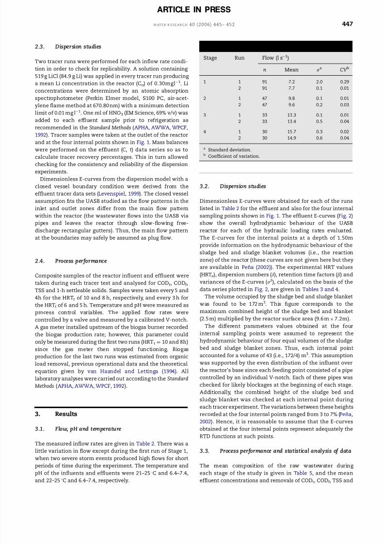
The measured inflow rates are given in Table 2. There was a

little variation in flow except during the first run of Stage 1,

when two severe storm events produced high flows for short

periods of time during the experiment. The temperature and

pH of the influents and effluents were 21–25 1C and 6.4–7.4,

and 22–25 1C and 6.4–7.4, respectively.

3.2. Dispersion studies

Dimensionless E-curves were obtained for each of the runs

listed in Table 2 for the effluent and also for the four internal

sampling points shown in Fig. 1. The effluent E-curves (Fig. 2)

show the overall hydrodynamic behaviour of the UASB

reactor for each of the hydraulic loading rates evaluated.

The E-curves for the internal points at a depth of 1.50m

provide information on the hydrodynamic behaviour of the

sludge bed and sludge blanket volumes (i.e., the reaction

zone) of the reactor (these curves are not given here but they

are available in Pen ˜ a (2002)). The experimental HRT values

(HRTe), dispersion numbers (d), retention time factors (b) and

variances of the E-curves (s2), calculated on the basis of the

data series plotted in Fig. 2, are given in Tables 3 and 4.

The volume occupied by the sludge bed and sludge blanket

was found to be 172 m3. This figure corresponds to the

maximum combined height of the sludge bed and blanket

(2.5 m) multiplied by the reactor surface area (9.6 m7.2m).

The different parameters values obtained at the four

internal sampling points were assumed to represent the

hydrodynamic behaviour of four equal volumes of the sludge

bed and sludge blanket zones. Thus, each internal point

accounted for a volume of 43 (i.e., 172/4) m3. This assumption

was supported by the even distribution of the influent over

the reactor’s base since each feeding point consisted of a pipe

controlled by an individual V-notch. Each of these pipes was

checked for likely blockages at the beginning of each stage.

Additionally, the combined height of the sludge bed and

sludge blanket was checked at each internal point during

each tracer experiment. The variations between these heights

recorded at the four internal points ranged from 3 to 7% (Pen ˜ a,

2002). Hence, it is reasonable to assume that the E-curves

obtained at the four internal points represent adequately the

RTD functions at such points.

3.3. Process performance and statistical analysis of data

The mean composition of the raw wastewater during

each stage of the study is given in Table 5, and the mean

effluent concentrations and removals of CODt, CODf , TSS and

ARTICLE IN PRESS

Table 2 – Hydraulic loading rate data

Stage Run Flow (l s1)

n Mean sa CV b

1 1 91 7.2 2.0 0.29

2 91 7.7 0.1 0.01

2 1 47 9.8 0.1 0.01

2 47 9.6 0.2 0.03

3 1 33 13.3 0.1 0.01

2 33 13.4 0.5 0.04

4 1 30 15.7 0.3 0.02

2 30 14.9 0.6 0.04

a Standard deviation.b Coefficient of variation.

W AT E R R E S E A R C H 40 (2006) 445– 452 447



ARTICLE IN PRESS

Table 3 – Summary of hydrodynamic parameters obtained at the reactor outlet

Stage Run Li+a (%) HRTtb (h) HRTe

c (h) b d Pe ( ¼ 1/d) V up (m h1) Hsbd (m) Q b

e (m3 h1)

1 1 72 10.6 7.0 0.66 0.163 6.1 0.38 1.2 1.6

2 70 9.9 5.8 0.59 0.145 6.9 0.41 1.4 3.1

2 1 68 7.8 4.9 0.63 0.197 5.1 0.52 1.9 2.2

2 60 7.9 5.4 0.68 0.185 5.4 0.51 1.9 3.8

3 1 95 5.7 5.8 1.01 0.720 1.4 0.70 2.6 4.8

2 93 5.7 6.3 1.10 0.591 1.7 0.71 2.6 6.4

4 1 90 4.9 4.3 0.88 0.355 2.8 0.83 3.2 5.7

2 87 5.1 4.8 0.94 0.406 2.5 0.79 3.1 5.1

a Percentages of tracer recovery (Li+) calculated from the E-curves.b Theoretical values based on hydraulic loading rates applied (see Table 3).c Experimental values.d Combined height of the sludge bed and sludge blanket taken from Pen ˜ a (2002).e Biogas production rate estimated from organic load removal during each run and from the equations given by Pen ˜ a (2002) and Samson and

Guiot (1985).

1.601.401.201.000.800.600.400.200.00

0.00 1.00 2.00 3.00 4.00

E

( θ ) = C / C o

θ = t/HRTt

E

( θ ) = C / C o

E

( θ ) = C / C o

E

( θ ) = C / C o

θ = t/HRTt θ = t/HRTt

θ = t/HRTt

Run 1

Duplicate

CSTR

Duplicate

CSTR

Duplicate

CSTRDuplicate

CSTR

1.40

1.20

1.00

0.80

0.60

0.40

0.20

0.000.00 0.50 1.00 1.50 2.00 2.50 3.00 3.50

HRT = 6 hHRT = 10 h

Run 3

1.601.401.201.000.800.600.400.200.00

0.00 1.00 2.00 3.00 4.00

Run 2

HRT = 8 h 1.20

1.00

0.80

0.60

0.40

0.20

0.000.00 1.00 2.00 3.00 4.00

Run 4

HRT = 5 h

Fig. 2 – Dimensionless E-curves obtained for the UASB effluent.

Table 4 – Summary of hydrodynamic parameters obtained at internal points 1–4

Stage: 1 2 3 4

Run: 1 2 1 2 1 2 1 2

HRTt (h) 6.6 6.2 4.9 4.9 3.6 3.6 3.1 3.2

Point 1 HRTe (h) 6.2 4.7 4.2 4.9 4.0 4.4 3.6 3.6

s2 0.595 0.348 0.504 0.649 0.644 0.552 0.545 0.554

d 0.553 0.223 0.397 0.685 0.671 0.472 0.461 0.475

Point 2 HRTe (h) 6.1 4.6 2.9 3.7 3.3 3.7 2.8 3.0

s2 0.636 0.436 0.211 0.571 0.683 0.569 0.529 0.560

d 0.649 0.311 0.120 0.507 0.789 0.502 0.434 0.487

Point 3 HRTe (h) 5.6 4.6 3.2 4.0 3.5 3.9 2.7 3.1

s2 0.578 0.381 0.357 0.543 0.634 0.532 0.529 0.558

d 0.519 0.254 0.231 0.456 0.644 0.438 0.435 0.483

Point 4 HRTe (h) 5.7 5.0 4.0 4.7 4.1 4.2 3.6 3.7

s2 0.603 0.379 0.488 0.586 0.712 0.545 0.538 0.529

d 0.571 0.252 0.374 0.536 0.894 0.460 0.448 0.434

W AT E R R E S E A R C H 4 0 ( 2 0 0 6 ) 4 4 5 – 4 5 2448



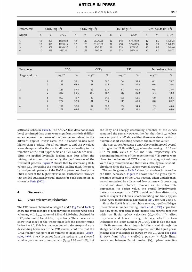
settleable solids in Table 6. The ANOVA test (data not shown

here) confirmed that there were significant statistical differ-

ences between the means of the parameters related to the

different applied inflow rates: the F-statistic values were

higher than F-critical for all parameters, and the p values

were always smaller than a in all cases, so leading to the

rejection of the null hypothesis at a 95% confidence level.

Thus the applied hydraulic loading rate does affect the

mixing pattern and consequently the performance of the

treatment process. Figure 2 shows that by decreasing HRTt

values (i.e., increasing the hydraulic loading rate), the gross

hydrodynamic pattern of the UASB approaches closely the

CSTR model at the highest flow value. Furthermore, Tukey’s

test yielded statistically equal means for each parameter, as

shown by Pen ˜ a (2002).

4. Discussion

4.1. Gross hydrodynamic behaviour

The RTD curves obtained for stages 1 and 2 (Fig. 2 and Table 3)

show the typical shape of a poorly mixed reactor with dead

volumes, with Epeak values of 1.50 and 1.40 being obtained for

HRTt values of 10.6 and 7.8h, respectively. These curves also

show that most of the tracer mass left the reactor much

before y ¼ 1.0. This feature, together with the steep and early

descending branches of the RTD curves, confirms that the

UASB reactor had part of its volume as dead space (Leven-

spiel, 1999). The RTD curves from the replicate runs showed

smaller peak values in comparison (Epeak 1.20 and 1.00), but

the early and sharply descending branches of the curves

remained the same. However, the fact that the Epeak values

were early and41.00 showed that there was also a fraction of

hydraulic short-circuiting between the inlet and outlet.

The RTD curves for stages 3 and 4 show an improved overall

mixing in the UASB, with Epeak values decreasing to 1.17 and

0.97 for HRTt values of 5.7 and 4.9h, respectively. The

descending branches of the experimental RTD curves were

closer to the theoretical CSTR curve; thus, stagnant volumes

were likely minimized and there was little hydraulic short-

circuiting since the Epeak values were all around 1.0.

The results given in Table 3 show that d values increased as

the HRTt decreased. Figure 2 shows that the gross hydro-

dynamic behaviour of the UASB reactor, when underloaded,

was characterised by a dispersed flow pattern with coexisting

mixed and dead volumes. However, as the inflow rate

approached its design value, the overall hydrodynamic

pattern converged to a CSTR model and flow distortions,

such as stagnant volumes, short-circuiting and likely bypass

flows, were minimized as depicted in Fig. 2 for runs 3 and 4.

Since the UASB is a three-phase reactor, liquid–solid–gas

interactions influence mixing. Iliuta et al. (1998) argue that

gas flow rates, especially in the bubble flow regime, together

with low liquid upflow velocities (V upo3 0 mh1), affect

dispersion and hence mixing intensity, which in turn

influences the Peclet number (Pe ¼ 1=d). This is also the case

in UASB reactors since biogas bubbles travel through the

sludge bed and sludge blanket together with the liquid phase

moving at low velocities as shown by the V up values in Table

3. Data from Table 4 yielded a positive multiple linear

correlation between Peclet number (Pe), upflow velocities

ARTICLE IN PRESS

Table 5 – Average composition of the raw wastewater throughout the study

Parameter: CODt (mg l1) CODf (mg l1) TSS (mg l1) Settl. solids (ml l1)

Stage: n ¯ y s=CV n ¯ y s=CV n ¯ y s=CV n ¯ y s=CV

1 12 398 152/0.38 12 143 55.2/0.38 12 148 57.5/0.39 12 1.5 1.1/0.73

2 12 396 182/0.46 12 120 79.7/0.66 12 218 57.6/0.26 12 2.3 1.6/0.69

3 10 509 189/0.37 10 162 35/0.22 10 235 87/0.37 10 2.6 1.2/0.464 10 559 82/0.15 10 167 74/0.44 10 272 56/0.20 10 3.7 1.0/0.27

Table 6 – Mean effluent concentrations and removals of CODt , CODf , TSS and settleable solids per run

Parameter: CODt CODf TSS Settleable solids

Stage and run: mg l1 % mg l1 % mg l1 % mg l1 %

1 1 153 52.1 71 56.0 54 55.8 0.2 70.7

2 159 64.8 47 63.8 74 57.2 0.4 74.4

2 1 144 57.5 42 57.4 81 65.0 0.5 75.6

2 283 52.6 105 45.4 143 36.3 1.4 42.2

3 1 259 48.7 85 54.8 101 61.1 1.0 60.4

2 272 52.9 81 53.7 145 61.4 0.8 84.7

4 1 289 50.6 62 60.8 204 34.5 2.5 45.8

2 279 48.6 101 55.3 180 39.0 1.7 45.0

W AT E R R E S E A R C H 40 (2006) 445– 452 449



(V up, m h1) and biogas production rates (Q b, m3 h1). The

equation obtained was

Pe ¼ 10:3 8:4V up 0:3Q b ðr2 ¼ 0:81Þ. (1)

This confirms that mixing intensity in UASBs is a function of

both liquid upflow velocity and biogas production rates (Bolle

et al., 1986; Iliuta et al., 1998).

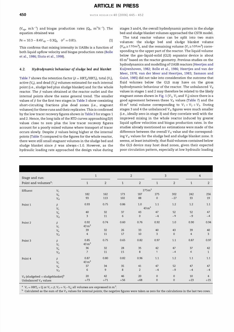
4.2. Hydrodynamic behaviour of sludge bed and blanket

Table 7 shows the retention factor (b ¼ HRTe /HRTt), total (V t),

active (V a), and dead (V d) volumes estimated for each internal

point (i.e., sludge bed plus sludge blanket) and for the whole

reactor. The b values obtained at the reactor outlet and the

internal points show the same general trend. The smaller

values of b for the first two stages in Table 3 show coexisting

short-circuiting fractions plus dead zones (i.e., stagnant

volumes) for these runs and their replicates. This is confirmed

by the low tracer recovery figures shown in Table 3 for stages 1

and 2. Hence, the long tails of the RTD curves approaching E(y)

values close to zero plus the low tracer recovery figures

account for a poorly mixed volume where transport of tracer

occurs slowly. Despite b values being higher at the internal

points (Table 7) compared to the figures for the whole reactor,

there were still small stagnant volumes in the sludge bed and

sludge blanket since b was alwayso1.0. However, as the

hydraulic loading rate approached the design value during

stages 3 and 4, the overall hydrodynamic pattern in the sludge

bed and sludge blanket volumes approached the CSTR model.

The total reactor volume can be split into two main

volumes: the sludge bed and sludge blanket volume

(V sbffi170m3), and the remaining volume (V rffi105m3) corre-

sponding to the upper part of the reactor. The liquid volume

below the gas–liquid–solid (GLS) separator device is about

65 m3 based on the reactor geometry. Previous studies on the

hydrodynamics and modelling of UASB reactors (Heertjes and

Kuijvenhoven, 1982; Bolle et al., 1986; Heertjes and van der

Meer, 1978; van der Meer and Heertjes, 1983; Samson and

Guiot, 1985) did not take into consideration the outcome that

fluid volumes below the GLS may have on the gross

hydrodynamic behaviour of the reactor. The unbalanced V dvalues in stages 1 and 2 may therefore be related to the likely

stagnant zones shown in Fig. 1 (V 1, V 2 and V 3) since there is a

good agreement between these V d values (Table 7) and the

65 m3 total volume corresponding to V 1 þ V 2 þ V 3. During

stages 3 and 4 the unbalanced V d figures were much smaller

(i.e., ideally zero in stage 3) and they correlate well with the

improved mixing in the whole reactor induced by greater

liquid upflow velocities and biogas production rates. In the

studies already mentioned no estimations were made of the

difference between the overall V d value and the correspond-

ing V d values for the sludge bed and sludge blanket zone. It

seems, at least intuitively, that fluid volumes contained below

the GLS device may host dead zones, given their expected

poor circulation pattern, especially at low hydraulic loading

ARTICLE IN PRESS

Table 7 – Estimates of active and dead volumes in the UASB reactor

Stage and run: 1 2 3 4

Point and volumesa: 1 2 1 2 1 2 1 2

Effluent V t 275m3

V a 182 162 173 187 275 302 242 256

V d 93 113 102 88 0 27 33 19

Point 1 b 0.93 0.75 0.86 1.0 1.1 1.2 1.2 1.1

V t 43 m3

V a 40 32 37 43 47 52 52 47

V d 3 11 6 0 4 9 9 4

Point 2 b 0.92 0.74 0.60 0.76 0.92 1.0 0.90 0.94

V t 43 m3

V a 39 32 26 33 40 43 39 40

V d 4 11 17 10 3 0 4 3

Point 3 b 0.85 0.75 0.65 0.82 0.97 1.1 0.87 0.97

V t 43 m3

V a 36 32 28 35 42 47 37 42

V d 7 11 15 8 1 4 6 1

Point 4 b 0.87 0.80 0.82 0.96 1.1 1.2 1.1 1.1

V t 43 m3

V a 37 34 35 41 47 52 47 47

V d 6 9 8 2 4 9 4 4

V d (sludgebed þ sludgeblanket)b 20 42 46 20 0 0 10 4

Unbalanced V d values þ73 þ71 þ56 þ68 0 0 þ23 þ15

a V a ¼ HRTeQ or V tb; V d ¼ V tV a; all volumes are expressed in m3.

b Calculated as the sum of the V d values for internal points; the negative figures were taken as zero for the calculations in the last two rows.

W AT E R R E S E A R C H 4 0 ( 2 0 0 6 ) 4 4 5 – 4 5 2450



and biogas production rates. However, more evidence from

full-scale UASBs is needed to prove this hypothesis.

Heertjes and van der Meer (1978) found that an increase in

the sludge height above 1.8 m improved the reactor efficiency,

but also increased the bypass flow over the sludge bed. The

results presented here are in agreement with these findings:

the negative values for V d in Table 7 obtained in stages 3 and 4

(i.e., for sludge heights42.6 m) confirm the existence of such

bypass flows. Run 2 in stage 3 showed bypass flows at three

internal points (negative figures) and these seemed to affect

the whole reactor given the negative overall V d figure

estimated from the outlet RTD curve. The hydrodynamic

behaviour improved dramatically once the reactor operated

close to its design conditions. Under these circumstances the

UASB closely approached the CSTR model with only a small

dead zone fraction (o5% V t plus high tracer recoveries);

similar results were obtained from other UASB reactors

treating domestic wastewater in Cali, Colombia (van Haandel

and Lettinga, 1994; Avella, 2001). However, dead zones

appeared again after the hydraulic loading rate was increased

beyond the design value (V d ¼ 10% V t), together with bypass

flows in the sludge bed and sludge blanket volumes. Hence,

the overloaded reactor was predominantly mixed but had an

intermediate dead zone and bypass flow in its lower part.

4.3. Process performance

The best removal efficiencies for CODt and CODf were

achieved between the end of stage 2 and the beginning of

stage 4 when the hydrodynamic performance of the reactor

showed a pattern close to the CSTR model. The improvement

of CODf removal efficiency could only be achieved through

better mixing and contact in the reaction zone (i.e., in the

sludge bed and sludge blanket) along with an extended

reaction time. Thus, improved mixing, more efficient mass

transfer processes (e.g., enhanced substrate transport from

the bulk liquid to the microbial aggregates) and longer HRTe

can be expected as the combined result of advection and

biogas induced mixing (i.e., combination of liquid upflow

velocity and biogas production rate). The same trend of the

removal efficiencies of CODt and CODf was also observed for

all the other parameters measured with the exception of

Settleable Solids.

These observations show that the reactor reached its

maximum efficiency when loaded optimally, that is, for

operational conditions close to the design scenario. A

consequence of this result is that UASB reactors exposed

directly to the random variation of wastewater flows (i.e.,

sewerage systems from human settlements or industrial

processes) may operate under different transient conditions

(i.e., underloaded, properly loaded and/or overloaded) at

various time periods. Therefore, the biological process

performance may not achieve steady-state conditions and

the overall efficiency will be reduced. UASBs are often

designed with short HRT values and so their capacity to

handle both underloading and overloading events is very

limited. In this work the UASB reactor had a constant-flow

pumping station upwaters and the applied hydraulic loadings

were well controlled.

Data from Tables 3 and 6 (d, effluent CODt, CODf and TSS,

respectively) yielded good logarithmic correlations, which are

given by the following equations

CODt-e ðmg =lÞ ¼ 78:27lnðdÞ þ 126 ðr2 ¼ 0:72Þ, (2)

TSSe ðmg =lÞ ¼ 66:53lnðdÞ þ 34:56 ðr2 ¼ 0:76Þ, (3)

CODf -e ðRem%Þ ¼ 7:27lnðdÞ þ 47:04 ðr2 ¼ 0:70Þ. (4)

These equations show a direct log-linear relationship

between the dispersion number (d) (i.e., hydrodynamics) and

the effluent concentrations of COD and TSS for the experi-

mental conditions tested herein. Although this may seem a

trivial result, the log-linear relationship essentially reveals

that the optimal hydrodynamic condition occurs somewhere

in between the two ideal flow extremes (i.e., plug flow and

complete mixing). Thus, the above equations seem to explain

reasonably well the relationship between the hydrodynamics

and the organic matter removal processes in the reactor

studied. Finally, as pointed out earlier, the ANOVA test also

showed that the variations in the applied hydraulic loading rate affected the hydrodynamic behaviour and consequently

the performance of the treatment process in the reactor.

5. Conclusions

1. The use of a combined dispersion-compartmental model

is an adequate tool to describe the macro-mixing proper-

ties of UASB reactors. The model showed that, when the

reactor was underloaded, there was a hydrodynamically

dispersed flow pattern with the coexistence of a well-

mixed fraction, stagnant zones and short-circuiting. The

main dead volumes were located in the sludge bed and

sludge blanket. Likewise, the liquid volume below the GLS

seemed to host a major stagnant zone not previously

reported elsewhere.

2. The UASB showed an ideal flow pattern (CSTR) for

operational conditions close to the design scenario.

However, both underloading and overloading events

produced distortions of the gross mixing behaviour with

predominantly arbitrary flow patterns.

3. Classical dispersion studies using inert tracers are ade-

quate to describe only the overall macro-mixing pattern in

UASB reactors, but they do not provide any additional

information on the diverse interactions between the

liquid, solid and gaseous phases, which are particularly

important in multiphase bioreactors treating complex

substrates.

4. Hydraulic loading rate variations altered the performance

of the treatment process in the reactor. However, the

correlations of the experimental data revealed that there is

an optimal zone to operate a UASB reactor hydraulically

(0.197o do0.720) in order to sustain its removal efficiency.

5. The implementation of simple engineering interventions

such as equalization tanks ahead of the UASB, will allow

for good handling of transient hydraulic loadings rates

while maintaining fairly constant operational conditions.

Additionally, the reactor can be designed for the average

flow and will not be unnecessarily big.

ARTICLE IN PRESS

W AT E R R E S E A R C H 40 (2006) 445– 452 451



Acknowledgement

The main author is indebted to COLCIENCIAS (Colombia) for

providing a scholarship for his doctoral training, which

included the experimental work reported herein.

R E F E R E N C E S

APHA, AWWA, WPCF, 1992. Standard Methods for the Examina-tion of Water and Wastewater, 18th ed. American PublicHealth Association, Washington, DC.

Avella, G.P., 2001. Evaluacion del Comportamiento Hidrodinamicode un Reactor UASB y su Influencia en la Remocion de MateriaOrganica (Evaluation of the hydrodynamic behaviour of anUASB reactor and its influence on organic matter removal).M.Sc. Dissertation, Universidad d el Valle/Instituto Cinara, Cali,Colombia.

Bailey, J.E., Ollis, D.F., 1986. Biochemical Engineering Fundamen-tals, second ed. McGraw-Hill, New York.

Bolle, W.L., van Breugel, J., van Eybergen, G.C., Koseen, N.W.F., vanGils, W., 1986. An integral dynamic model for the UASB reactor.Biotech. Bioeng. XXVIII, 1621–1636.

Heertjes, P.M., Kuijvenhoven, L.J., 1982. Fluid flow pattern inupflow reactors for anaerobic treatment of beet sugar factorywastewater. Biotech. Bioeng. XXIV, 443–459.

Heertjes, P.M., van der Meer, R.R., 1978. Dynamics of liquid flow inan up-flow reactor used for anaerobic treatment of waste-water. Biotech. Bioeng. XX, 1577–1594.

Iliuta, I., Thyrion, F.C., Muntean, O., 1998. Axial dispersion of liquid in gas–liquid co-current downflow and upflow fixed-bedreactors with porous particles. Trans. Chem. Eng. 76 (A), 64–72.

Kvanli, A.H., Pavur, R.J., Guynes, C.S., 2000. Introduction toBusiness Statistics, fifth ed. South-Western College Publish-ing, Cincinnati, OH.

Levenspiel, O., 1999. Chemical Reaction Engineering, third ed.Wiley, New York.

Montgomery, D.C., 1997. Design and Analysis of Experiments,fourth ed. Wiley, New York.

Ottino, J.M., 1990. Mixing, chaotic advection, and turbulence.Annu. Rev. Fluid. Mech. 22, 207–254.

Ottino, J.M., Khakhar, D.V., 2000. Mixing and segregation of granular materials. Annu. Rev. Fluid. Mech. 32, 55–91.

Pen ˜ a, M.R., 2002. Advanced primary treatment of domestic waste-water in tropical countries: development of high-rate anaerobicponds. Ph.D. Thesis, University of Leeds, Leeds, England.

Samson, R., Guiot, S., 1985. Mixing characteristics and perfor-mance of the anaerobic upflow blanket filter (UBF) reactor. J.Chem. Tech. Biotechnol. 35 (B), 65–74.

van der Meer, R.R., Heertjes, P.M., 1983. Mathematical descriptionof anaerobic treatment of wastewater in upflow reactors.Biotech. Bioeng. XXV, 2557–2566.

van Haandel, A.C., Lettinga, G., 1994. Anaerobic Sewage Treat-ment: A Practical Guide for Regions with a Hot Climate. Wiley,Chichester, England.

ARTICLE IN PRESS

W AT E R R E S E A R C H 4 0 ( 2 0 0 6 ) 4 4 5 – 4 5 2452

Documents

Dispersion and Tretament Perfomance Analysis of an UASB Reactor Under Different Hydraulic Loading Rates