Dispersive Quantization ofLinear and Nonlinear Waves

Peter J. Olver

University of Minnesota

http://www.math.umn.edu/∼ olver

Durham — July, 2016

Peter J. OlverIntroduction to Partial Differential Equations

Undergraduate Texts, Springer, 2014

—, Dispersive quantization, Amer. Math. Monthly117 (2010) 599–610.

Gong Chen & —, Dispersion of discontinuous periodic waves,Proc. Roy. Soc. London A 469 (2012), 20120407.

Gong Chen & —, Numerical simulation of nonlineardispersive quantization, Discrete Cont. Dyn. Syst. A34 (2013), 991–1008.

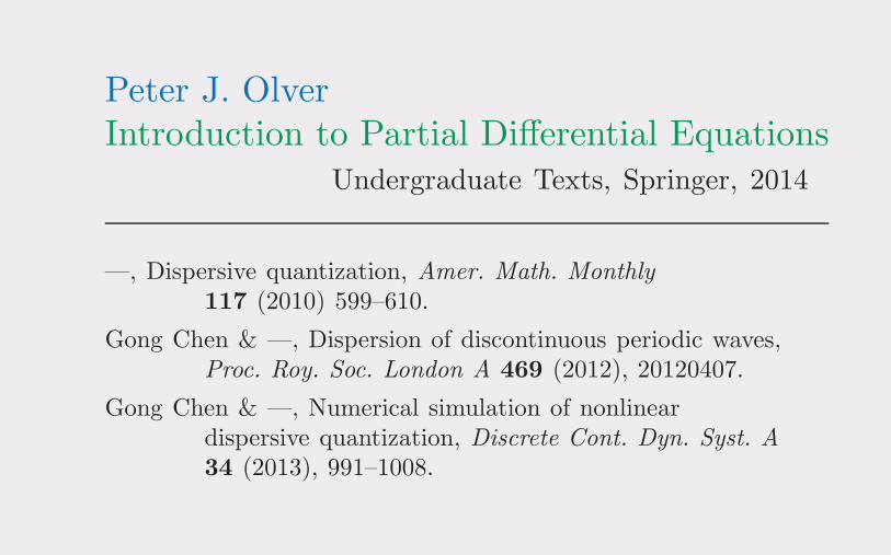
Dispersion

Definition. A linear partial differential equation is calleddispersive if the different Fourier modes travel unalteredbut at different speeds.

Substitutingu(t, x) = e i (kx−ω t)

produces the dispersion relation

ω = ω(k), ω, k ∈ R

relating frequency ω and wave number k.

Phase velocity: cp =ω(k)

k

Group velocity: cg =dω

dk(stationary phase)

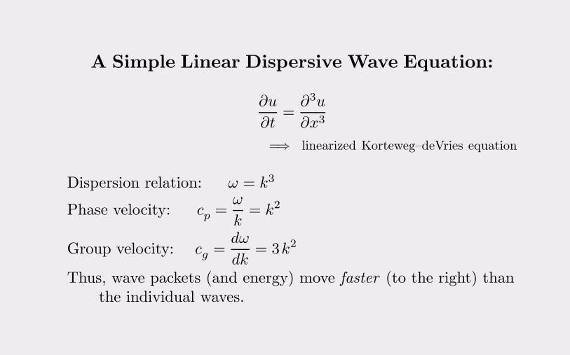
A Simple Linear Dispersive Wave Equation:

∂u

∂t=∂3u

∂x3

=⇒ linearized Korteweg–deVries equation

Dispersion relation: ω = k3

Phase velocity: cp =ω

k= k2

Group velocity: cg =dω

dk= 3k2

Thus, wave packets (and energy) move faster (to the right) thanthe individual waves.

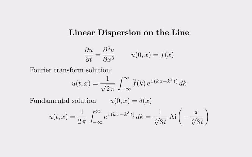
Linear Dispersion on the Line

∂u

∂t=∂3u

∂x3u(0, x) = f(x)

Fourier transform solution:

u(t, x) =1√2π

∫ ∞

−∞f(k) e i (kx−k3 t) dk

Fundamental solution u(0, x) = δ(x)

u(t, x) =1

2π

∫ ∞

−∞e i (kx−k3 t) dk =

13√3 t

Ai

(

−x

3√3 t

)

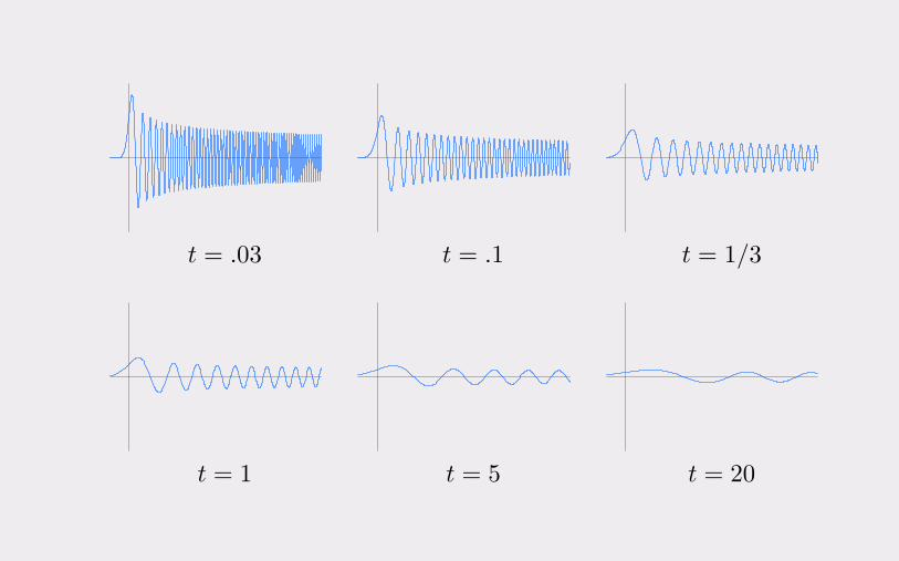
t = .03 t = .1 t = 1/3

t = 1 t = 5 t = 20

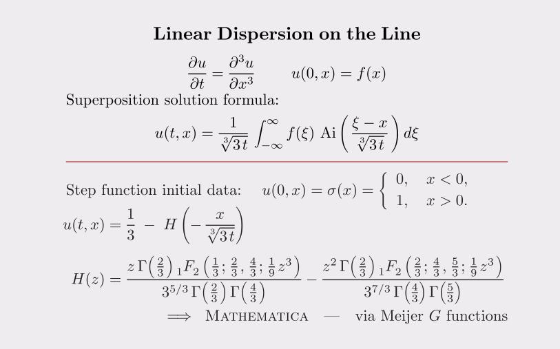
Linear Dispersion on the Line

∂u

∂t=∂3u

∂x3u(0, x) = f(x)

Superposition solution formula:

u(t, x) =1

3√3 t

∫ ∞

−∞f(ξ) Ai

(ξ − x3√3 t

)

dξ

Step function initial data: u(0, x) = σ(x) =

{0, x < 0,

1, x > 0.

u(t, x) =1

3− H

(

−x

3√3 t

)

H(z) =z Γ

(23

)1F2

(13 ;

23 ,

43 ;

19 z

3)

35/3 Γ(23

)Γ(43

) −z2 Γ

(23

)1F2

(23 ;

43 ,

53 ;

19 z

3)

37/3 Γ(43

)Γ(53

)

=⇒ Mathematica — via Meijer G functions

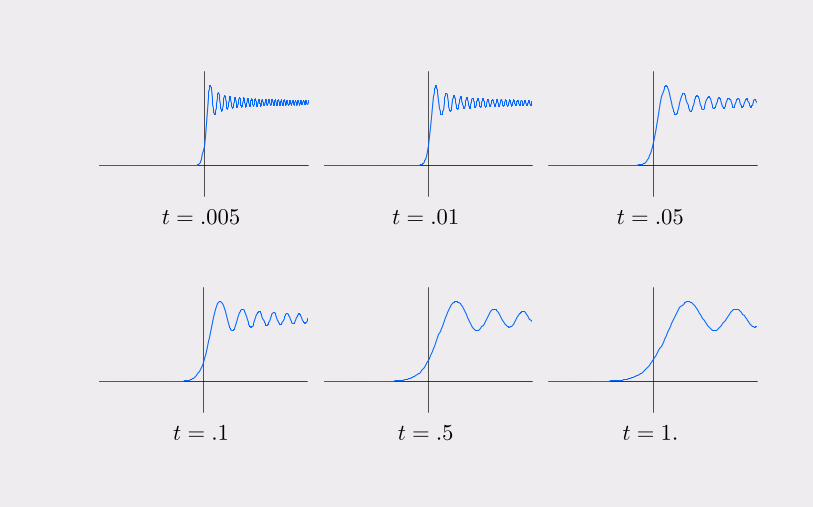
t = .005 t = .01 t = .05

t = .1 t = .5 t = 1.

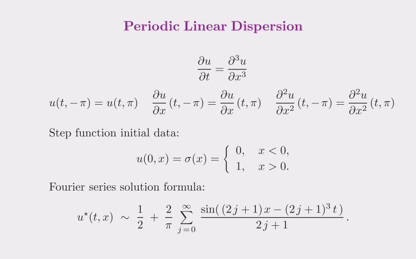
Periodic Linear Dispersion

∂u

∂t=∂3u

∂x3

u(t,−π) = u(t,π)∂u

∂x(t,−π) =

∂u

∂x(t,π)

∂2u

∂x2(t,−π) =

∂2u

∂x2(t,π)

Step function initial data:

u(0, x) = σ(x) =

{0, x < 0,

1, x > 0.

Fourier series solution formula:

u⋆(t, x) ∼1

2+

2

π

∞∑

j=0

sin( (2j + 1)x− (2j + 1)3 t )

2j + 1.

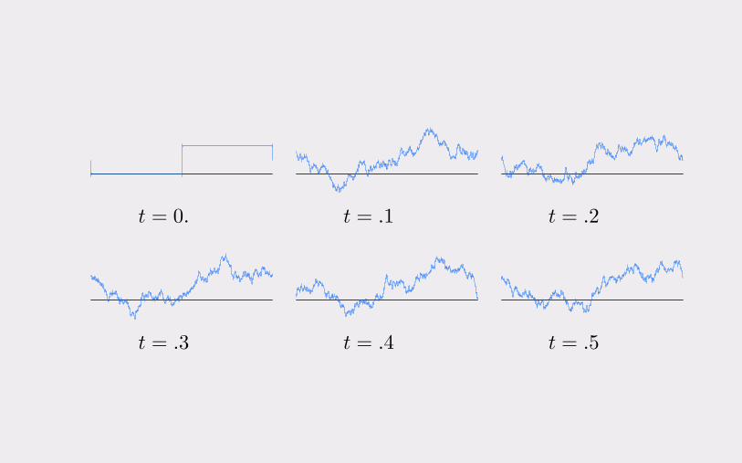
t = 0. t = .1 t = .2

t = .3 t = .4 t = .5

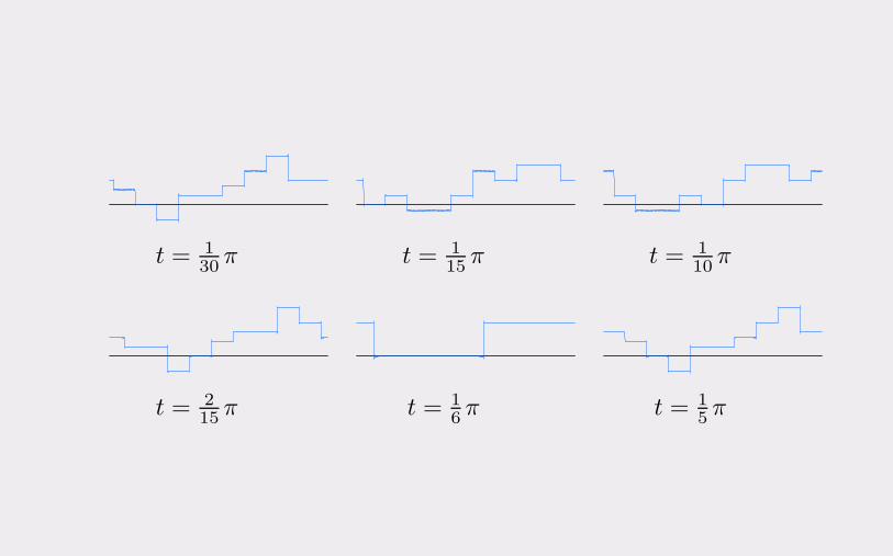
t = 130 π t = 1

15 π t = 110 π

t = 215 π t = 1

6 π t = 15 π

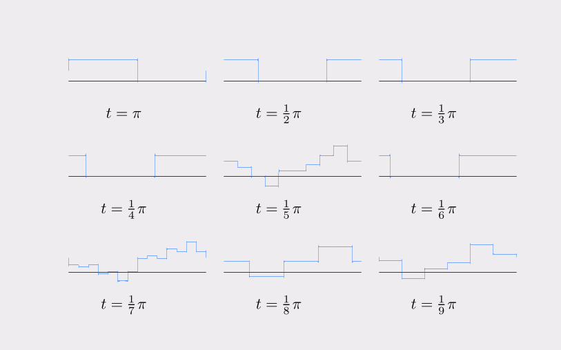
t = π t = 12 π t = 1

3 π

t = 14 π t = 1

5 π t = 16 π

t = 17 π t = 1

8 π t = 19 π

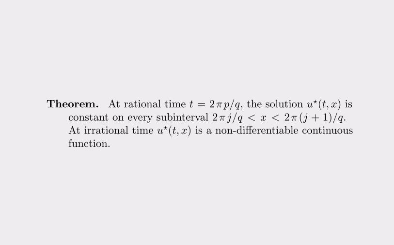
Theorem. At rational time t = 2πp/q, the solution u⋆(t, x) isconstant on every subinterval 2π j/q < x < 2π (j + 1)/q.At irrational time u⋆(t, x) is a non-differentiable continuousfunction.

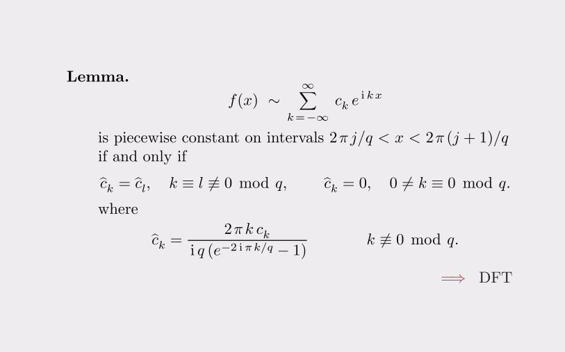
Lemma.

f(x) ∼∞∑

k=−∞

ck ei kx

is piecewise constant on intervals 2π j/q < x < 2π (j + 1)/qif and only if

ck = cl, k ≡ l ≡ 0 mod q, ck = 0, 0 = k ≡ 0 mod q.

where

ck =2πk ck

i q (e−2 iπk/q − 1)k ≡ 0 mod q.

=⇒ DFT

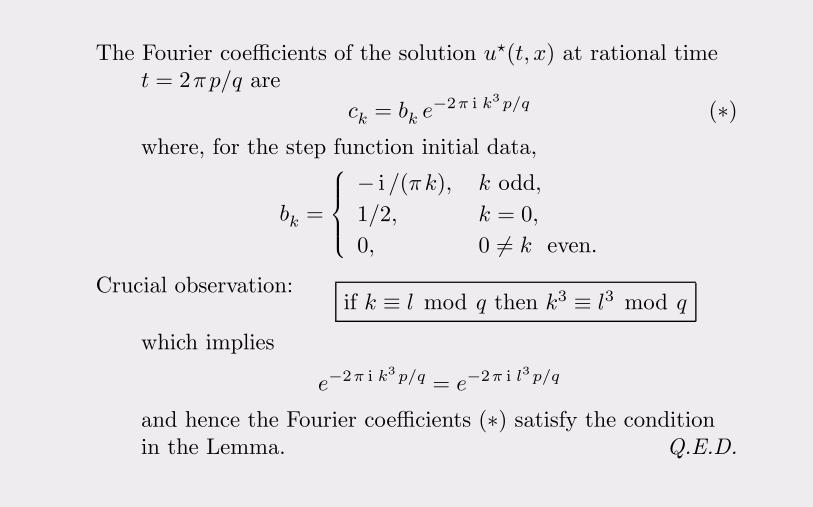
The Fourier coefficients of the solution u⋆(t, x) at rational timet = 2πp/q are

ck = bk e−2π i k3p/q (∗)

where, for the step function initial data,

bk =

⎧⎪⎪⎨

⎪⎪⎩

− i /(πk), k odd,

1/2, k = 0,

0, 0 = k even.

Crucial observation:if k ≡ l mod q then k3 ≡ l3 mod q

which implies

e−2π i k3 p/q = e−2π i l3p/q

and hence the Fourier coefficients (∗) satisfy the conditionin the Lemma. Q.E.D.

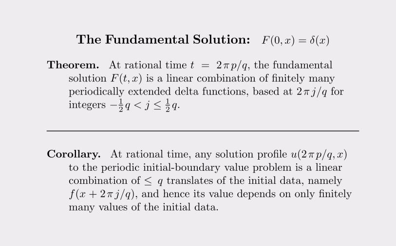
The Fundamental Solution: F (0, x) = δ(x)

Theorem. At rational time t = 2πp/q, the fundamentalsolution F (t, x) is a linear combination of finitely manyperiodically extended delta functions, based at 2π j/q forintegers −1

2 q < j ≤ 12 q.

Corollary. At rational time, any solution profile u(2πp/q, x)to the periodic initial-boundary value problem is a linearcombination of ≤ q translates of the initial data, namelyf(x + 2π j/q), and hence its value depends on only finitelymany values of the initial data.

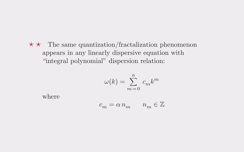
⋆ ⋆ The same quantization/fractalization phenomenonappears in any linearly dispersive equation with“integral polynomial” dispersion relation:

ω(k) =n∑

m=0

cmkm

wherecm = αnm nm ∈ Z

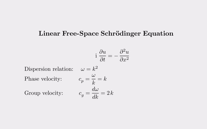
Linear Free-Space Schrodinger Equation

i∂u

∂t= −

∂2u

∂x2

Dispersion relation: ω = k2

Phase velocity: cp =ω

k= k

Group velocity: cg =dω

dk= 2k

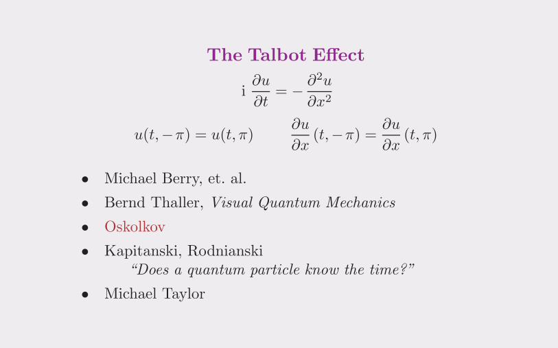
The Talbot Effect

i∂u

∂t= −

∂2u

∂x2

u(t,−π) = u(t,π)∂u

∂x(t,−π) =

∂u

∂x(t,π)

• Michael Berry, et. al.

• Bernd Thaller, Visual Quantum Mechanics

• Oskolkov

• Kapitanski, Rodnianski“Does a quantum particle know the time?”

• Michael Taylor

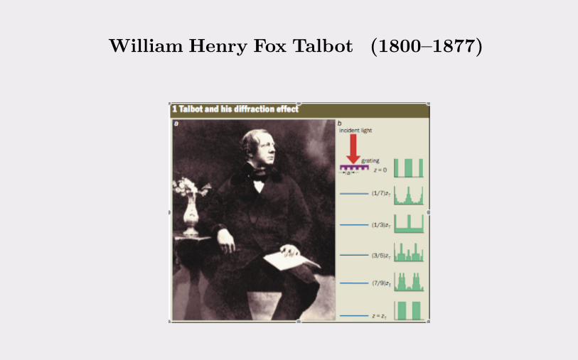
William Henry Fox Talbot (1800–1877)

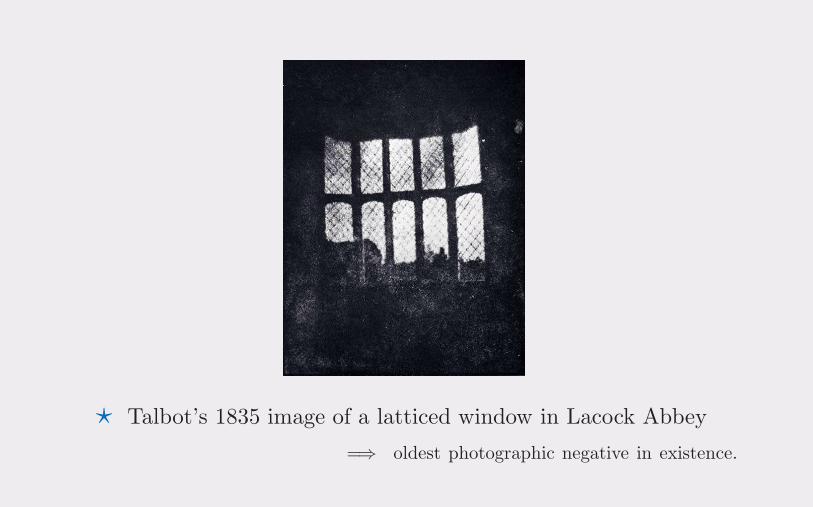
⋆ Talbot’s 1835 image of a latticed window in Lacock Abbey

=⇒ oldest photographic negative in existence.

ATalbot Experiment

Fresnel diffraction by periodic gratings (1836):

“It was very curious to observe that though the grating wasgreatly out of the focus of the lens . . . the appearance ofthe bands was perfectly distinct and well defined . . . theexperiments are communicated in the hope that they mayprove interesting to the cultivators of optical science.”

— Fox Talbot

=⇒ Lord Rayleigh calculates the Talbot distance (1881)

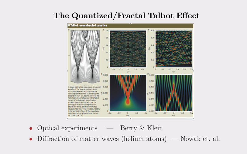
The Quantized/Fractal Talbot Effect

• Optical experiments — Berry & Klein

• Diffraction of matter waves (helium atoms) — Nowak et. al.

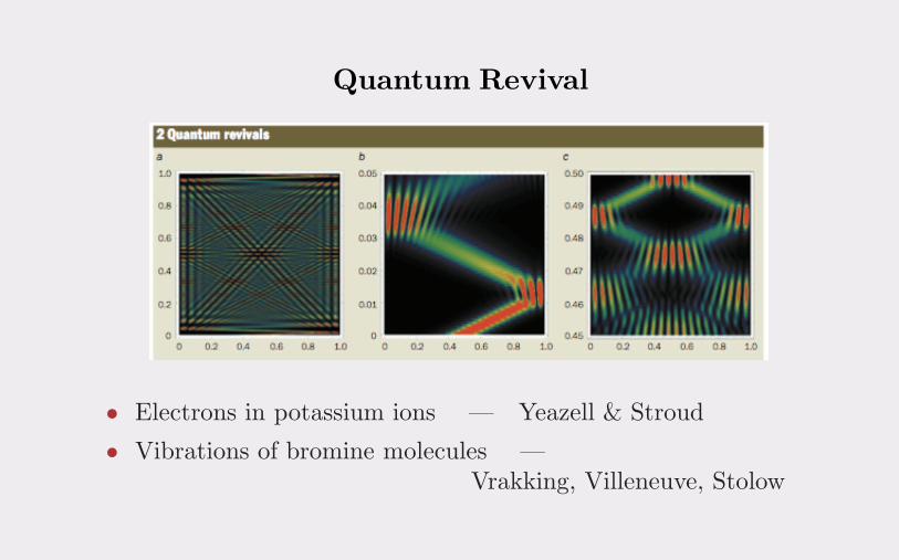
Quantum Revival

• Electrons in potassium ions — Yeazell & Stroud

• Vibrations of bromine molecules —Vrakking, Villeneuve, Stolow

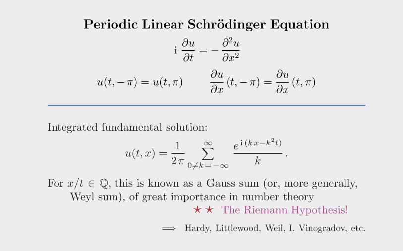
Periodic Linear Schrodinger Equation

i∂u

∂t= −

∂2u

∂x2

u(t,−π) = u(t,π)∂u

∂x(t,−π) =

∂u

∂x(t,π)

Integrated fundamental solution:

u(t, x) =1

2π

∞∑

0=k=−∞

e i (kx−k2t)

k.

For x/t ∈ Q, this is known as a Gauss sum (or, more generally,Weyl sum), of great importance in number theory

⋆ ⋆ The Riemann Hypothesis!

=⇒ Hardy, Littlewood, Weil, I. Vinogradov, etc.

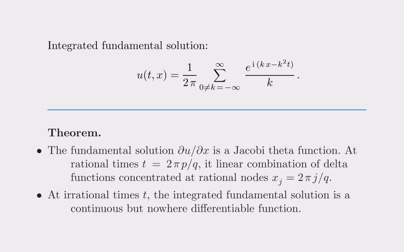
Integrated fundamental solution:

u(t, x) =1

2π

∞∑

0=k=−∞

e i (kx−k2t)

k.

Theorem.

• The fundamental solution ∂u/∂x is a Jacobi theta function. Atrational times t = 2πp/q, it linear combination of deltafunctions concentrated at rational nodes xj = 2π j/q.

• At irrational times t, the integrated fundamental solution is acontinuous but nowhere differentiable function.

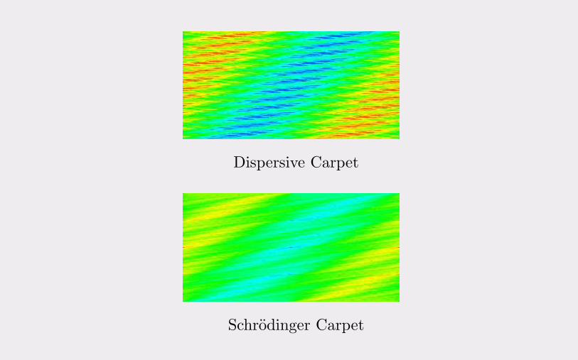
Dispersive Carpet

Schrodinger Carpet

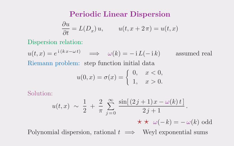
Periodic Linear Dispersion∂u

∂t= L(Dx) u, u(t, x+ 2π) = u(t, x)

Dispersion relation:

u(t, x) = e i (kx−ω t) =⇒ ω(k) = − iL(− i k) assumed real

Riemann problem: step function initial data

u(0, x) = σ(x) =

{0, x < 0,

1, x > 0.

Solution:

u(t, x) ∼1

2+

2

π

∞∑

j=0

sin[ (2j + 1)x− ω(k) t ]

2j + 1.

⋆ ⋆ ω(−k) = −ω(k) odd

Polynomial dispersion, rational t =⇒ Weyl exponential sums

2DWaterWaves

h

y = h+ η(t, x) surface elevation

φ(t, x, y) velocity potential

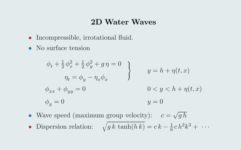
2D Water Waves

• Incompressible, irrotational fluid.

• No surface tension

φt +12 φ

2x +

12 φ

2y + g η = 0

ηt = φy − ηxφx

⎫⎬

⎭ y = h+ η(t, x)

φxx + φyy = 0 0 < y < h+ η(t, x)

φy = 0 y = 0

• Wave speed (maximum group velocity): c =√g h

• Dispersion relation:√g k tanh(h k) = c k − 1

6 c h2k3 + · · ·

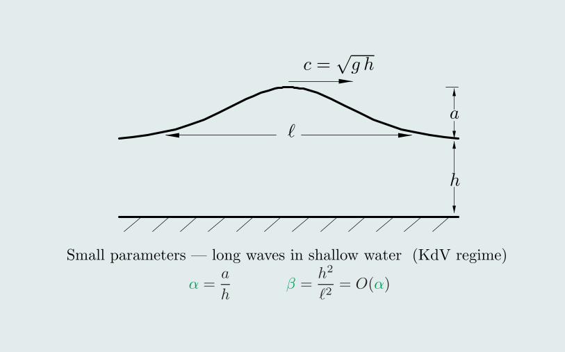
h

aℓ

c =√g h

Small parameters — long waves in shallow water (KdV regime)

α =a

hβ =

h2

ℓ2= O(α)

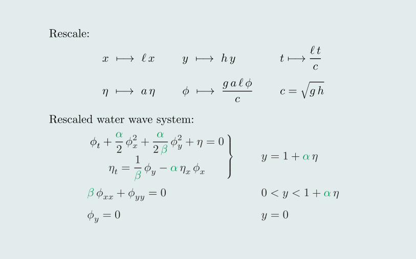
Rescale:

x *−→ ℓ x y *−→ h y t *−→ℓ t

c

η *−→ a η φ *−→g a ℓ φ

cc =

√g h

Rescaled water wave system:

φt +α

2φ2x +

α

2βφ2y + η = 0

ηt =1

βφy − α ηx φx

⎫⎪⎪⎬

⎪⎪⎭y = 1 + αη

β φxx + φyy = 0 0 < y < 1 + α η

φy = 0 y = 0

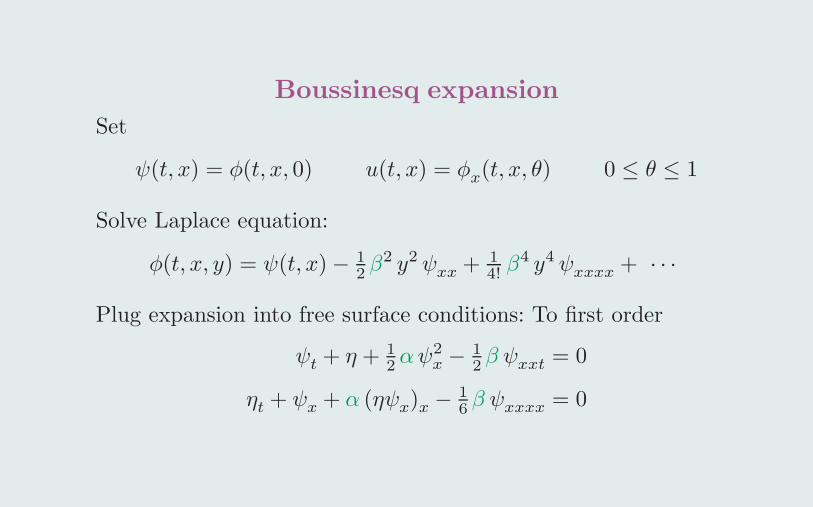
Boussinesq expansion

Set

ψ(t, x) = φ(t, x, 0) u(t, x) = φx(t, x, θ) 0 ≤ θ ≤ 1

Solve Laplace equation:

φ(t, x, y) = ψ(t, x)− 12 β

2 y2 ψxx +14! β

4 y4 ψxxxx + · · ·

Plug expansion into free surface conditions: To first order

ψt + η + 12αψ

2x −

12 β ψxxt = 0

ηt + ψx + α (ηψx)x −16 β ψxxxx = 0

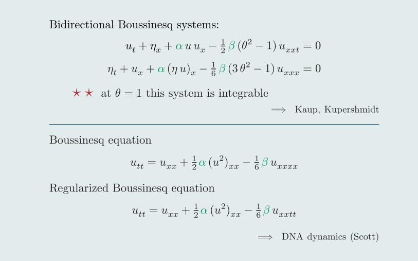
Bidirectional Boussinesq systems:

ut + ηx + α uux −12 β (θ

2 − 1)uxxt = 0

ηt + ux + α (η u)x −16 β (3 θ

2 − 1)uxxx = 0

⋆ ⋆ at θ = 1 this system is integrable

=⇒ Kaup, Kupershmidt

Boussinesq equation

utt = uxx +12α (u2)xx −

16 β uxxxx

Regularized Boussinesq equation

utt = uxx +12α (u2)xx −

16 β uxxtt

=⇒ DNA dynamics (Scott)

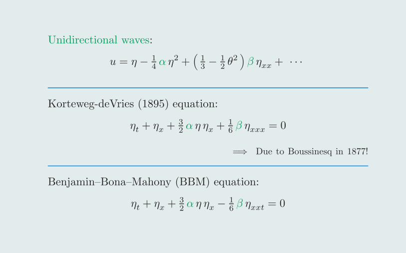
Unidirectional waves:

u = η − 14 αη

2 +(

13 −

12 θ

2)β ηxx + · · ·

Korteweg-deVries (1895) equation:

ηt + ηx +32 α η ηx +

16 β ηxxx = 0

=⇒ Due to Boussinesq in 1877!

Benjamin–Bona–Mahony (BBM) equation:

ηt + ηx +32 αη ηx −

16 β ηxxt = 0

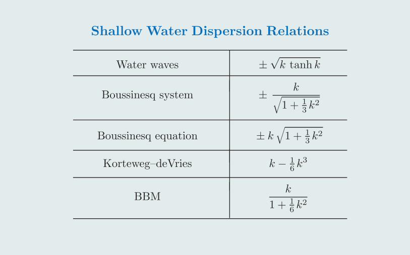
Shallow Water Dispersion Relations

Water waves ±√k tanh k

Boussinesq system ±k

√1 + 1

3 k2

Boussinesq equation ± k√1 + 1

3 k2

Korteweg–deVries k − 16 k

3

BBMk

1 + 16 k

2

Dispersion Asymptotics

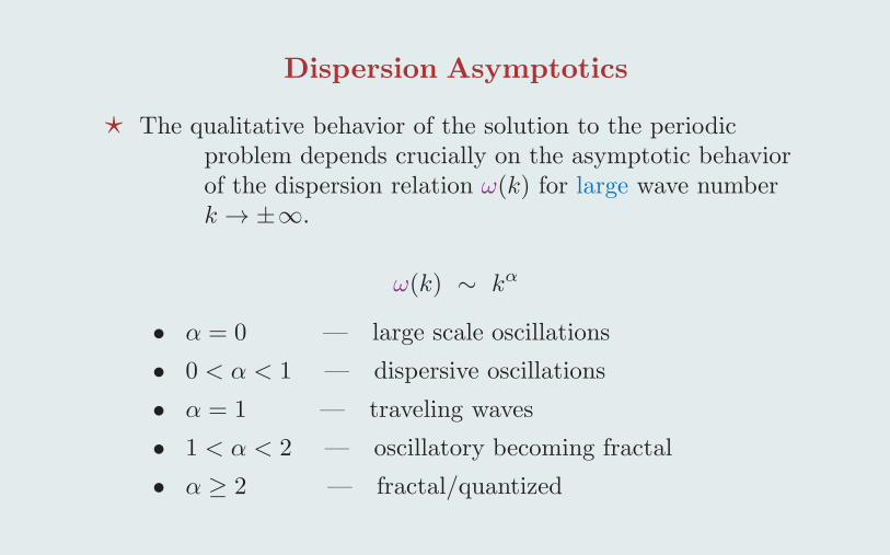
⋆ The qualitative behavior of the solution to the periodicproblem depends crucially on the asymptotic behaviorof the dispersion relation ω(k) for large wave numberk → ±∞.

ω(k) ∼ kα

• α = 0 — large scale oscillations

• 0 < α < 1 — dispersive oscillations

• α = 1 — traveling waves

• 1 < α < 2 — oscillatory becoming fractal

• α ≥ 2 — fractal/quantized

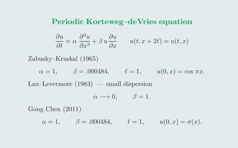
Periodic Korteweg–deVries equation

∂u

∂t= α

∂3u

∂x3+ β u

∂u

∂xu(t, x+ 2ℓ) = u(t, x)

Zabusky–Kruskal (1965)

α = 1, β = .000484, ℓ = 1, u(0, x) = cos πx.

Lax–Levermore (1983) — small dispersion

α −→ 0, β = 1.

Gong Chen (2011)

α = 1, β = .000484, ℓ = 1, u(0, x) = σ(x).

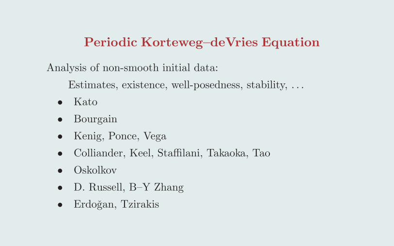
Periodic Korteweg–deVries Equation

Analysis of non-smooth initial data:

Estimates, existence, well-posedness, stability, . . .

• Kato

• Bourgain

• Kenig, Ponce, Vega

• Colliander, Keel, Staffilani, Takaoka, Tao

• Oskolkov

• D. Russell, B–Y Zhang

• Erdogan, Tzirakis

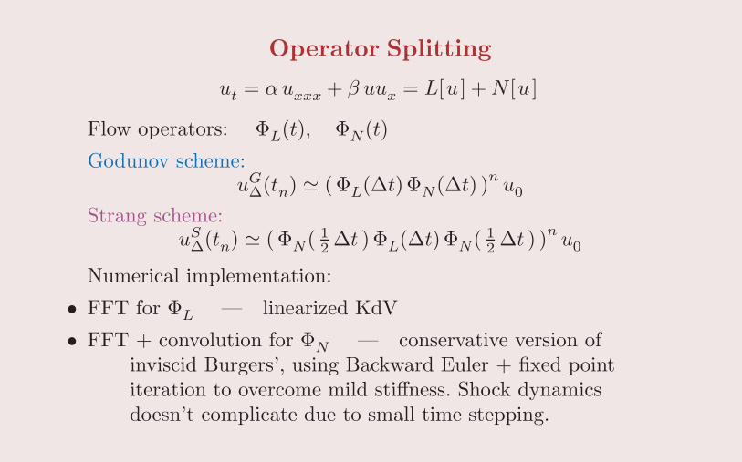
Operator Splitting

ut = αuxxx + β uux = L[u ] +N [u ]

Flow operators: ΦL(t), ΦN(t)

Godunov scheme:uG∆(tn) ≃ (ΦL(∆t)ΦN(∆t) )n u0

Strang scheme:uS∆(tn) ≃ (ΦN( 1

2 ∆t )ΦL(∆t)ΦN( 12 ∆t ) )n u0

Numerical implementation:

• FFT for ΦL — linearized KdV

• FFT + convolution for ΦN — conservative version ofinviscid Burgers’, using Backward Euler + fixed pointiteration to overcome mild stiffness. Shock dynamicsdoesn’t complicate due to small time stepping.

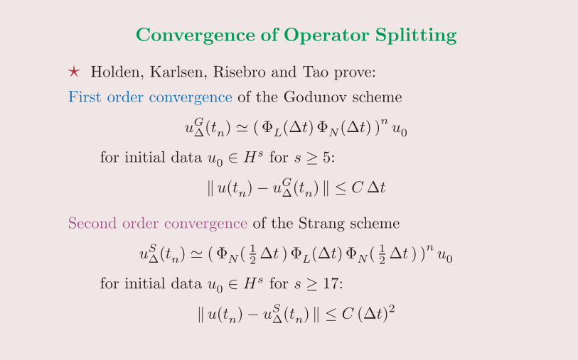
Convergence of Operator Splitting

⋆ Holden, Karlsen, Risebro and Tao prove:

First order convergence of the Godunov scheme

uG∆(tn) ≃ (ΦL(∆t)ΦN(∆t) )n u0

for initial data u0 ∈ Hs for s ≥ 5:

∥u(tn)− uG∆(tn) ∥ ≤ C∆t

Second order convergence of the Strang scheme

uS∆(tn) ≃ (ΦN( 1

2 ∆t )ΦL(∆t)ΦN( 12 ∆t ) )n u0

for initial data u0 ∈ Hs for s ≥ 17:

∥u(tn)− uS∆(tn) ∥ ≤ C (∆t)2

Convergence for Rough Data?

However, subtle issues prevent us from establishing convergence of theoperator splitting method for rough initial data.

• Bourgain proves well-posedness of the periodic KdV flow in L2

• Conservation of the L2 norm establishes well-posedness in L2 of the linearizedflow ΦL

• Thus, if the solution has bounded L∞ norm, then the linearized flow is L1

contractive

• Oskolkov proves that is the initial data is has bounded BV norm, then theresulting solution to the periodic linearized KdV equation is uniformlybounded in L∞

• Unfortunately, Oskolkov’s bound depends on the BV and L∞ norms of theinitial data. Moreover, at irrational times, the solution is nowheredifferentiable and has unbounded BV norm

• Also, we do not have good control of the BV norm of the nonlinear inviscidBurgers’ flow ΦN

• ????

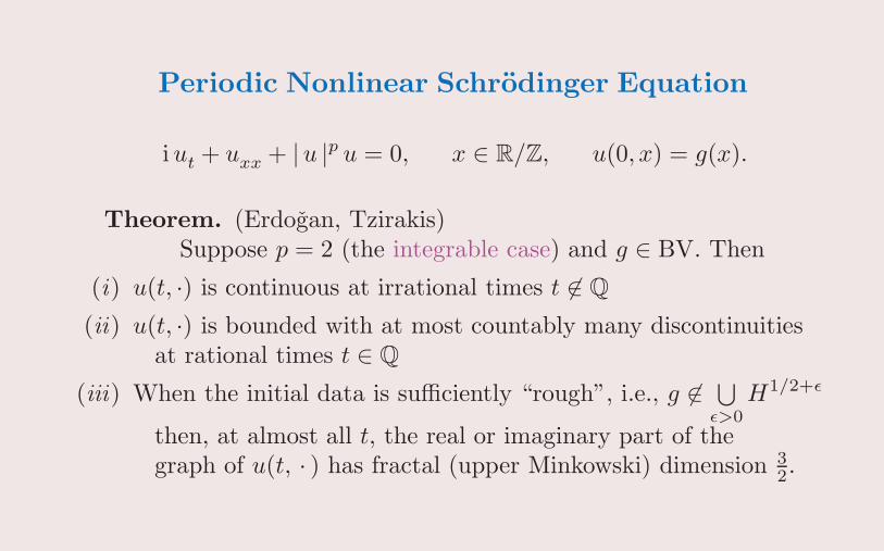
Periodic Nonlinear Schrodinger Equation

iut + uxx + |u |p u = 0, x ∈ R/Z, u(0, x) = g(x).

Theorem. (Erdogan, Tzirakis)Suppose p = 2 (the integrable case) and g ∈ BV. Then

(i) u(t, ·) is continuous at irrational times t ∈ Q

(ii) u(t, ·) is bounded with at most countably many discontinuitiesat rational times t ∈ Q

(iii) When the initial data is sufficiently “rough”, i.e., g ∈!

ϵ>0H1/2+ϵ

then, at almost all t, the real or imaginary part of thegraph of u(t, · ) has fractal (upper Minkowski) dimension 3

2.

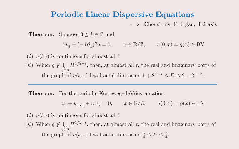
Periodic Linear Dispersive Equations=⇒ Chousionis, Erdogan, Tzirakis

Theorem. Suppose 3 ≤ k ∈ Z and

iut + (− i ∂x)ku = 0, x ∈ R/Z, u(0, x) = g(x) ∈ BV

(i) u(t, ·) is continuous for almost all t

(ii) When g ∈!

ϵ>0H1/2+ϵ, then, at almost all t, the real and imaginary parts of

the graph of u(t, · ) has fractal dimension 1 + 21−k ≤ D ≤ 2− 21−k.

Theorem. For the periodic Korteweg–deVries equation

ut + uxxx + uux = 0, x ∈ R/Z, u(0, x) = g(x) ∈ BV

(i) u(t, ·) is continuous for almost all t

(ii) When g ∈!

ϵ>0H1/2+ϵ, then, at almost all t, the real and imaginary parts of

the graph of u(t, · ) has fractal dimension 54 ≤ D ≤ 7

4 .

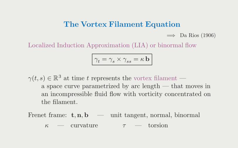
The Vortex Filament Equation=⇒ Da Rios (1906)

Localized Induction Approximation (LIA) or binormal flow

γt = γs × γss = κb

γ(t, s) ∈ R3 at time t represents the vortex filament —a space curve parametrized by arc length — that moves inan incompressible fluid flow with vorticity concentrated onthe filament.

Frenet frame: t,n,b — unit tangent, normal, binormal

κ — curvature τ — torsion

γt = γs × γss

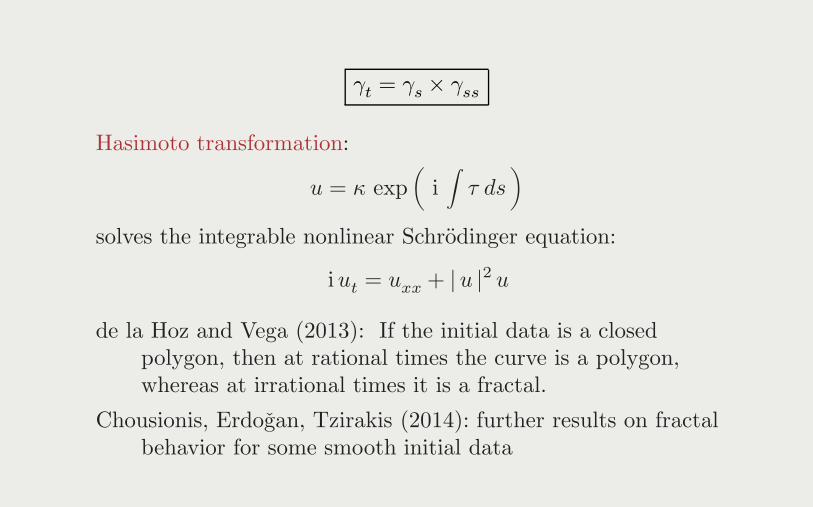
Hasimoto transformation:

u = κ exp(i∫τ ds

)

solves the integrable nonlinear Schrodinger equation:

iut = uxx + |u |2 u

de la Hoz and Vega (2013): If the initial data is a closedpolygon, then at rational times the curve is a polygon,whereas at irrational times it is a fractal.

Chousionis, Erdogan, Tzirakis (2014): further results on fractalbehavior for some smooth initial data

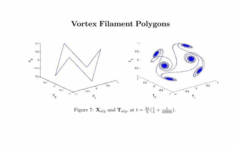
Vortex Filament Polygons

Figure 7: Xalg and Talg, at t =2π

9( 14+ 1

49999).

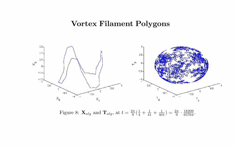
Vortex Filament Polygons

Figure 8: Xalg and Talg, at t =2π

9( 14+ 1

41+ 1

401) = 2π

9·18209

65764.

Future Directions

• General dispersion behavior

• Other boundary conditions (Fokas’ Method)

• Higher space dimensions and other domains(tori, spheres, . . . )

• Dispersive nonlinear partial differential equations

• Discrete systems: Fermi–Pasta–Ulam

• Numerical solution techniques?

• Experimental verification in dispersive media?