DISPLACEMENT, CONFLICT AND WELFARE: AN EMPIRICAL ANALYSIS. A PROGRESS REPORT BY O.ATTANASIO C.CASTRO AND A. MESNARD

OUTLINE

June 2005

I Introduction

II determinants of household migration decision

1. Motivation of the empirical model

11 traditional literature

12 violence and migration

13 impact of welfare programmes on migration

2. Data

21 sample

22 household level variables

23 municipality level variables

3. Results

31 main results

32 Robustness checks

33 Does violence incidence interact with the programme effect ?

34 Does violence incidence modify household incentives to migrate ?

III Consequences of migration

1 Consequences of mobility: evidence from the FA special module on the successfully

tracked households

11 reasons for migration

12 intentions to move again in the future

13 migration benefits and costs

2 Consequences of displacement: evidence from a survey on displacement

21 motivations and data

22 migration history of displaced households

23 comparing movers and stayers

24 how do displaced households cope with poverty?

3 Comparison of displaced and non-displaced households

31 How do displaced households differ from the poor households in the FA sample?

32 How do displaced households differ from the households interviewed for FA and that

migrated out of their municipalities of origin?

IV conclusion and policy implications

Appendix

I Introduction

Colombia’s civil conflict over the last 40 years has displaced many families and

individuals from their villages of origin. Estimates vary, but it is clear that the problem

has become, especially in recent decades, a very important one. Casual visits to the main

cities in Colombia provide abundant evidence of the problem: displaced individuals are

visible in poor neighbourhoods and more generally on the streets. The consequence of

such displacement can be dramatic. In addition to the direct act of violence that causes

the displacement, individuals often loose their livehood, productive assets and valuable

skills, the human capital they possess is often inadequate in the new environments,

children are removed from school and so and so forth.

The study of the consequences of displacement in Colombia has often used data on

individuals or households that have been displaced from the villages of origin and that

have emerged somewhere else, typically in a large city. This, however, is only part of the

story. Many individuals do not leave the region of origin and decide to stay in the village

of origin. This report is the first study, to the best of our knowledge, that complements

the existing studies by looking at individuals who live in the same villages of origin of

the displaced but, for some reason, are not displaced. These data are then compared with

those of a more traditional survey which gathers information on displaced individuals and

families. In particular, our research approach is to:

1. Characterize displacement and mobility. Using a first data source, we can

characterize which households move from their original village and why and

distinguish those that we can follow to a new location and those we cannot track

down. In Sections III.2 and III.3, we compare the demographic and economic

profile of the households in this first data source (both those who move and those

who do not) to the profile of ‘displaced households’ in other data sets collected in

recipient municipalities.

2. Relate the observed mobility to several environmental factors, as reported in

Section II. These include:

a. Municipality data on infrastructure and social capital collected in the

locality questionnaires added to the survey

b. Retrospective information on violence and displacement at the

municipality level.

c. The presence (or not) of the programme Familias en Acción that could

have diminished the level of mobility.

3. Study the consequences of mobility and displacement, as reported in Sections

III.1 and III.2.

As we mentioned above, the most innovative aspect of this research is the study of

households who, while living in the same villages and areas from which displaced

households leave to reach the big Colombian cities, do not leave these areas. This

innovation was possible because of the availability of a large and high quality data set,

whose collection was started in 2002 with the purpose of evaluating a new welfare

programme, called Familias en Acción, run by the Colombian government with a loan

from the IADB and the World Bank. The programme is modelled after the Mexican

PROGRESA and consists of conditional cash transfers that aim at improving the nutrition

and education of the poorest Colombians. The survey collected information on 11,500

households living in 122 (relatively small) municipalities, 57 of which were targeted by

the new programme and 65 of which were not. The first data collection (which we refer

to as the baseline data) was done just before the start of the new programme.1

We thought that such a survey, if suitably expanded, could be used to study displacement

and mobility. For the second data collection, which was executed in 2003, we therefore

decided to add several modules to the basic questionnaire (which was already very rich).

In particular, we invested a considerable amount of resources to track down households

that had moved from the baseline survey and, to these households, a newly designed

module on mobility was administered. Second, we constructed extensive locality

questionnaires that were administered to three ‘local’ authorities (such as the mayor, the

1 The evaluation and the survey were organized by a consortium made of Econometria, IFS and SEI. In some of the ‘treatment’ towns, the programme was started by the government before the baseline survey. These issues and the baseline data are discussed in detail in Attanasio et al. (2004).

programme official and the priest). Third, we tried a novel way to measure social capital

by means of experimental games in 12 of the 122 towns in our sample.

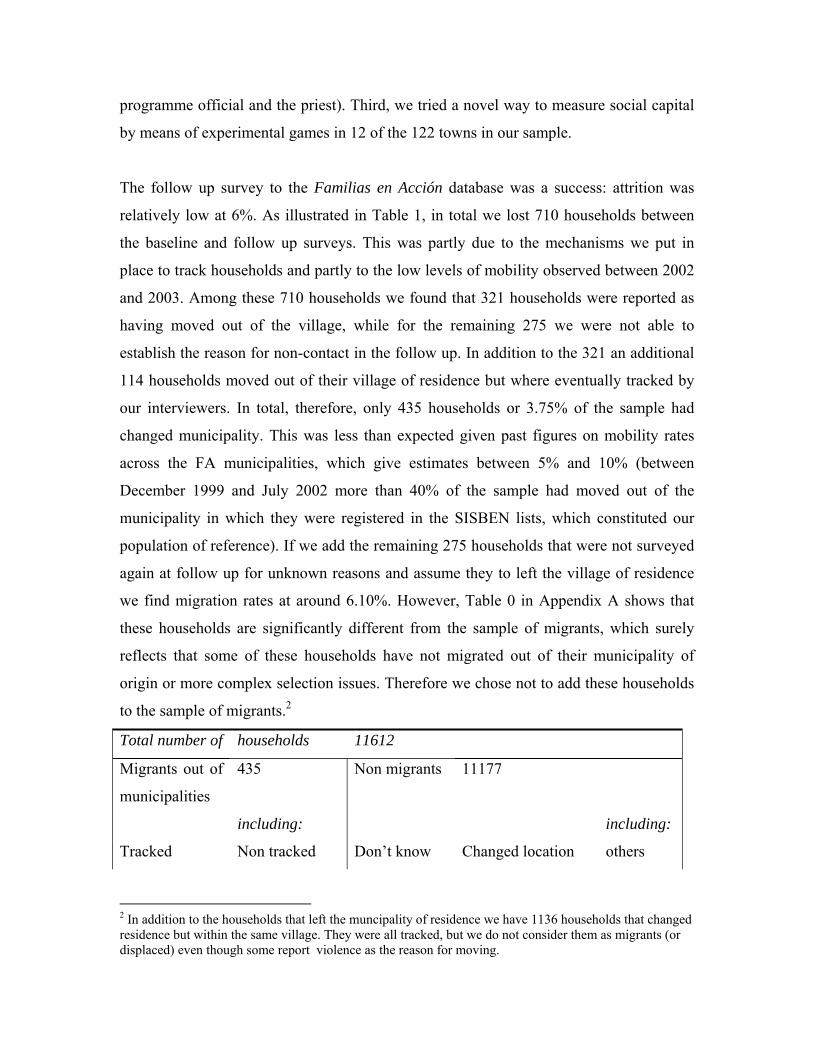
The follow up survey to the Familias en Acción database was a success: attrition was

relatively low at 6%. As illustrated in Table 1, in total we lost 710 households between

the baseline and follow up surveys. This was partly due to the mechanisms we put in

place to track households and partly to the low levels of mobility observed between 2002

and 2003. Among these 710 households we found that 321 households were reported as

having moved out of the village, while for the remaining 275 we were not able to

establish the reason for non-contact in the follow up. In addition to the 321 an additional

114 households moved out of their village of residence but where eventually tracked by

our interviewers. In total, therefore, only 435 households or 3.75% of the sample had

changed municipality. This was less than expected given past figures on mobility rates

across the FA municipalities, which give estimates between 5% and 10% (between

December 1999 and July 2002 more than 40% of the sample had moved out of the

municipality in which they were registered in the SISBEN lists, which constituted our

population of reference). If we add the remaining 275 households that were not surveyed

again at follow up for unknown reasons and assume they to left the village of residence

we find migration rates at around 6.10%. However, Table 0 in Appendix A shows that

these households are significantly different from the sample of migrants, which surely

reflects that some of these households have not migrated out of their municipality of

origin or more complex selection issues. Therefore we chose not to add these households

to the sample of migrants.2

Total number of households 11612

Migrants out of

municipalities

435

Non migrants

11177

including: including:

Tracked Non tracked Don’t know Changed location others

2 In addition to the households that left the muncipality of residence we have 1136 households that changed residence but within the same village. They were all tracked, but we do not consider them as migrants (or displaced) even though some report violence as the reason for moving.

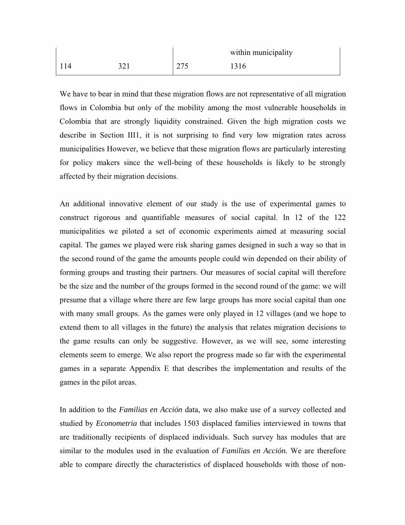
within municipality

114 321 275 1316

We have to bear in mind that these migration flows are not representative of all migration

flows in Colombia but only of the mobility among the most vulnerable households in

Colombia that are strongly liquidity constrained. Given the high migration costs we

describe in Section III1, it is not surprising to find very low migration rates across

municipalities However, we believe that these migration flows are particularly interesting

for policy makers since the well-being of these households is likely to be strongly

affected by their migration decisions.

An additional innovative element of our study is the use of experimental games to

construct rigorous and quantifiable measures of social capital. In 12 of the 122

municipalities we piloted a set of economic experiments aimed at measuring social

capital. The games we played were risk sharing games designed in such a way so that in

the second round of the game the amounts people could win depended on their ability of

forming groups and trusting their partners. Our measures of social capital will therefore

be the size and the number of the groups formed in the second round of the game: we will

presume that a village where there are few large groups has more social capital than one

with many small groups. As the games were only played in 12 villages (and we hope to

extend them to all villages in the future) the analysis that relates migration decisions to

the game results can only be suggestive. However, as we will see, some interesting

elements seem to emerge. We also report the progress made so far with the experimental

games in a separate Appendix E that describes the implementation and results of the

games in the pilot areas.

In addition to the Familias en Acción data, we also make use of a survey collected and

studied by Econometria that includes 1503 displaced families interviewed in towns that

are traditionally recipients of displaced individuals. Such survey has modules that are

similar to the modules used in the evaluation of Familias en Acción. We are therefore

able to compare directly the characteristics of displaced households with those of non-

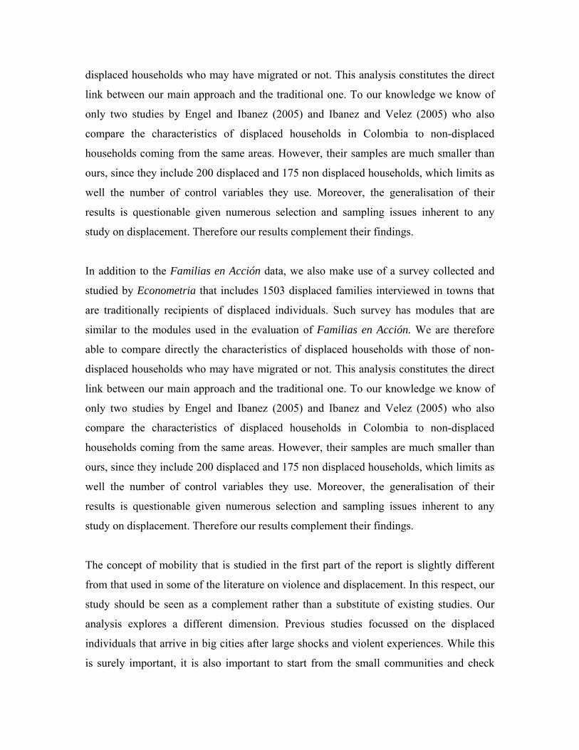
displaced households who may have migrated or not. This analysis constitutes the direct

link between our main approach and the traditional one. To our knowledge we know of

only two studies by Engel and Ibanez (2005) and Ibanez and Velez (2005) who also

compare the characteristics of displaced households in Colombia to non-displaced

households coming from the same areas. However, their samples are much smaller than

ours, since they include 200 displaced and 175 non displaced households, which limits as

well the number of control variables they use. Moreover, the generalisation of their

results is questionable given numerous selection and sampling issues inherent to any

study on displacement. Therefore our results complement their findings.

In addition to the Familias en Acción data, we also make use of a survey collected and

studied by Econometria that includes 1503 displaced families interviewed in towns that

are traditionally recipients of displaced individuals. Such survey has modules that are

similar to the modules used in the evaluation of Familias en Acción. We are therefore

able to compare directly the characteristics of displaced households with those of non-

displaced households who may have migrated or not. This analysis constitutes the direct

link between our main approach and the traditional one. To our knowledge we know of

only two studies by Engel and Ibanez (2005) and Ibanez and Velez (2005) who also

compare the characteristics of displaced households in Colombia to non-displaced

households coming from the same areas. However, their samples are much smaller than

ours, since they include 200 displaced and 175 non displaced households, which limits as

well the number of control variables they use. Moreover, the generalisation of their

results is questionable given numerous selection and sampling issues inherent to any

study on displacement. Therefore our results complement their findings.

The concept of mobility that is studied in the first part of the report is slightly different

from that used in some of the literature on violence and displacement. In this respect, our

study should be seen as a complement rather than a substitute of existing studies. Our

analysis explores a different dimension. Previous studies focussed on the displaced

individuals that arrive in big cities after large shocks and violent experiences. While this

is surely important, it is also important to start from the small communities and check

what happens to individuals that, while affected by violence and other problems, do not

necessarily move to the big cities but to other places or stay in the municipalities. These

decisions are not necessarily entirely forced but we expect them to be determined directly

by the high levels of violence in the municipalities. Studying whether and to what extent

the mobility of poor households is linked to the displacement process in Colombia will be

one focus of this report. We are also in the position to characterise the profile of the

individuals within the communities that are displaced versus migrants, as developed in

the second part of the report. In this respect our study is novel and unique and we think it

completes the knowledge from other studies in an important way.

The rest of the report is organized as follows. In section II we discuss the determinants of

household decision to leave its municipality of residence between the baseline and

follow-up FA surveys. In Section III we study the consequences of mobility and

displacement on the well-being of households. We also compare the households in the

FA data set to displaced households who are coming from the same rural municipalities.

Section IV concludes by establishing policy recommendations based on our main

findings.

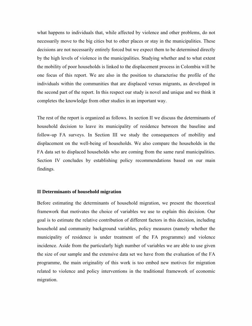
II Determinants of household migration Before estimating the determinants of household migration, we present the theoretical

framework that motivates the choice of variables we use to explain this decision. Our

goal is to estimate the relative contribution of different factors in this decision, including

household and community background variables, policy measures (namely whether the

municipality of residence is under treatment of the FA programme) and violence

incidence. Aside from the particularly high number of variables we are able to use given

the size of our sample and the extensive data set we have from the evaluation of the FA

programme, the main originality of this work is too embed new motives for migration

related to violence and policy interventions in the traditional framework of economic

migration.

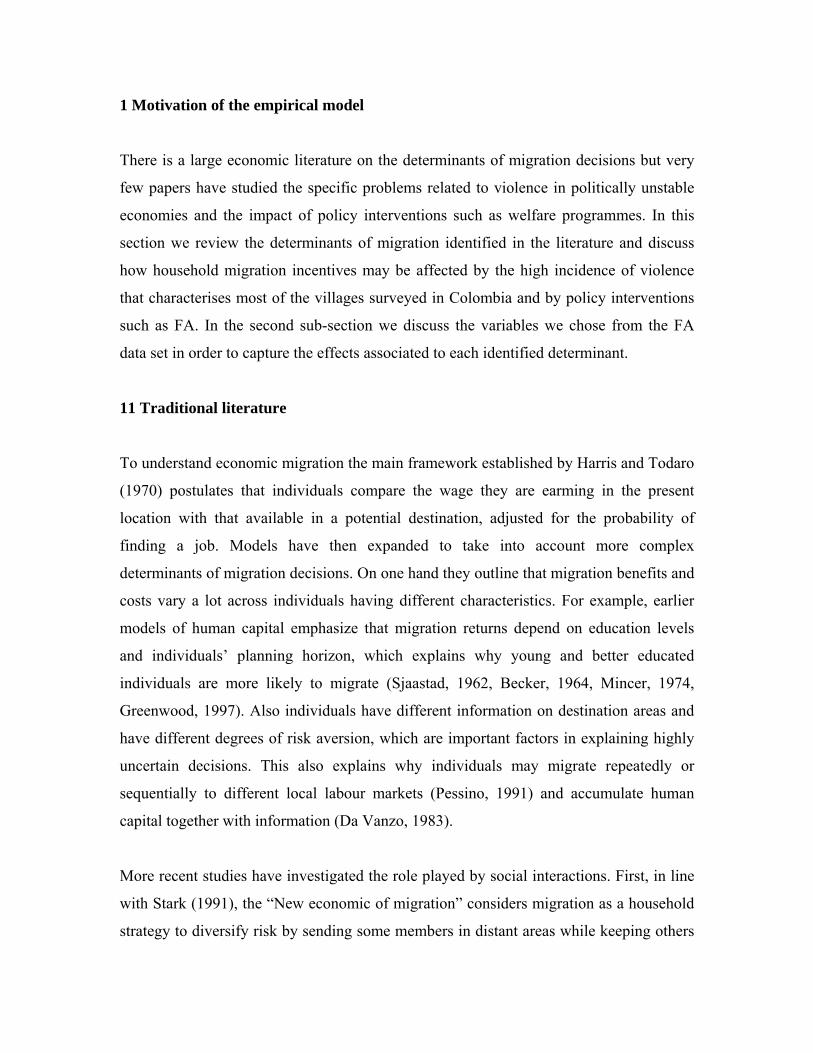
1 Motivation of the empirical model

There is a large economic literature on the determinants of migration decisions but very

few papers have studied the specific problems related to violence in politically unstable

economies and the impact of policy interventions such as welfare programmes. In this

section we review the determinants of migration identified in the literature and discuss

how household migration incentives may be affected by the high incidence of violence

that characterises most of the villages surveyed in Colombia and by policy interventions

such as FA. In the second sub-section we discuss the variables we chose from the FA

data set in order to capture the effects associated to each identified determinant.

11 Traditional literature

To understand economic migration the main framework established by Harris and Todaro

(1970) postulates that individuals compare the wage they are earming in the present

location with that available in a potential destination, adjusted for the probability of

finding a job. Models have then expanded to take into account more complex

determinants of migration decisions. On one hand they outline that migration benefits and

costs vary a lot across individuals having different characteristics. For example, earlier

models of human capital emphasize that migration returns depend on education levels

and individuals’ planning horizon, which explains why young and better educated

individuals are more likely to migrate (Sjaastad, 1962, Becker, 1964, Mincer, 1974,

Greenwood, 1997). Also individuals have different information on destination areas and

have different degrees of risk aversion, which are important factors in explaining highly

uncertain decisions. This also explains why individuals may migrate repeatedly or

sequentially to different local labour markets (Pessino, 1991) and accumulate human

capital together with information (Da Vanzo, 1983).

More recent studies have investigated the role played by social interactions. First, in line

with Stark (1991), the “New economic of migration” considers migration as a household

strategy to diversify risk by sending some members in distant areas while keeping others

working on farm. Then, sociologists have outlined that social networks have a strong

impact on the size of migration costs. For example, they help new immigrants in their job

and house search or by proposing them services (Massey, Alarcon, Durand and Gonzalez,

1987); they play a large role in mitigating the hazard of crossing the borders between

Mexico, and US (Espinosa and Massey, 1997 ); or they help migrants find higher paying

job upon arrival in the US (Munshi, 2003). As a result migration costs become

endogenous to the migration process as modelled by Carrington, Detragiache and

Vishwanath (1996).

In line with these models our analysis will take into account a set of economic factors that

push households out of their municipality of residence, together with household and

community characteristics that determine migration costs and benefits. Note that we do

not observe the destinations chosen by most of migrant households and therefore cannot

control for pull factors in the destination areas.3 Also we do not adopt the approach of the

“New economic of migration” and restrict our study to the household decision to migrate

as a whole unit given the limited information we have on the mobility of household

members.

12 Violence and migration

The economic literature on the impact of violence on migration is not very developed,

partly due to the scarcity of available data, partly because this field was left to political

scientists until very recently. However, in a seminal paper, Schultz (1971) finds a positive

effect of the incidence of homicides on net internal migration rates from 1951 to 1964 in

Colombia. Also, Morrison and May (1994) show that political violence is a key

determinant of internal migration rates in Guatemala. But using aggregate data, these

authors cannot capture easily the microeconomic underpinnings of household migration

decisions in violent context, which is the main objective of our study.

3 Only 135 households have been successfully tracked during the first follow up, which is a too small sample to test for the effects of “pull” factors.

However, in the last couple of years there has been a growing attention paid to the

consequences of civil war and conflicts on displacement and asylum seekers (see for

example Azam and Hoeffler, 2002, or Hatton, 2004). Although we may argue that forced

migration and economic migration are of different nature, we cannot exclude that these

two decisions have common factors. This may explain why, very often, only part of

households from communities targeted by illegal armed groups decide to move. To

capture this feature Engel and Ibanez (2005), or Ibanez and Velez (2005) extend the

expected utility framework developed by Morrison and May (1994) to explain

displacement decisions. This framework postulates that households leave their area of

origin when their utility to stay is smaller than utility to move, taking into account all

socio-political and economic benefits and costs attached to different locations. As a

result, predictions of such models are sometimes opposite to those of traditional

migration models. For example, households with immobile assets like large plots of land

that can be easily sized by rebels may feel more threatened by violence and, hence, are

encouraged to move first, contrary to what the standard economic literature would

predict. Similarly, risk aversion may induce individuals to displace in a violent context,

whereas the same individuals would not have migrated in a stable context, because of the

uncertainties involved by migration decisions (Fischer et al, 1997). Or individuals with

political responsibilities in their municipalities may be the first targeted by rebel or

paramilitary forces in their strategies to destabilise rural areas and take control over them.

This also outlines the complex role that social capital is likely to play in the migration

decision under violence. Then any advantage to belong to a society and may discourage

migration like active participation in community activities or high education levels may

also turn into a risk factor and encourage displacement, as studied by Ibanez and Velez

(2005).

In line with Morrison and May (1994) and the literature on displacement, our model of

migration will embed factors linked to violence into a framework of expected utility. To

capture the effect of violence on household well-being, we will enter different proxies

measuring the level of violence prevailing in the municipality of residence among the

explanatory variables of migration decisions. Furthermore, we will allow the level of

0violence to affect not only directly the well being of households attached to a given

location but also the migration incentives associated to other factors. This argument,

firstly outlined by Morrison and May (1994), has not been exploited further since.4 Using

micro-data we can test easily whether the effects associated to specific factors depend on

the level of violence by adding interaction terms between these factors and the level of

violence.

13 Impact of welfare programme on migration

Another important benefit attached to living in a municipality is whether its inhabitants

receive benefits from welfare programmes. However the literature on the impacts of

welfare programmes on migration is scant. To our knowledge only one paper by

Angelucci (2005) investigates the effect of the PROGRESA conditional cash transfer

programme in Mexico on international labour migration. However, the political and

economic context of Mexico where communities have experienced large international

migration flows in the past and formed important migration networks in the US is very

different from Colombia.

Although the FA programme has not been designed specifically to affect migration

behaviour, there are many ways in which household mobility might respond to it. On one

hand, receiving the benefits of the Familias en Accion programme makes living in a

municipality where the programme operates (hereafter “treatment municipality”) more

attractive than living in a municipality where it does not (“control municipality”).

Accordingly we expect a negative correlation between living in a treatment municipality

at baseline and the probability that a household migrates out of this municipality between

the baseline and follow up surveys. On the other hand, receiving cash transfers may also

help relaxing financial constraints of very poor households, and, hence, allow them to

finance their migration if migration returns are high as compared to its costs. Since these

4 Ibanez and al (2005)’s results show that the determinants of displacement are different from those of migration but, given the scope of the paper and their data, they do not test for how economic determinants are modified by the level of violence.

two effects play in opposite direction, the effect of receiving the programme on a

household mobility is a priori ambiguous.

We also expect the programme to affect differently migration decisions of households

depending on their characteristics and environment. In particular the incidence of

violence varies a lot across municipalities and the programme may affect differently

migration incentives of households depending on whether they are threatened by violence

or not. For example, by relaxing cash constraints, the programme may allow some

households threatened by violence to migrate, whereas these households would not

benefit from migrating in a stable environment. Or the programme may discourage

migration only if violence incidence is not unduly high. We also know that, in principle,

those benefiting from the programme may be different from those not benefiting from it.

In particular, large households with many small children aged less than 7 years old

receive larger amounts of cash transfers, as well as families with lots of children enrolled

in school. We will therefore test for possible interaction effects of the programme with

the violence levels in municipalities, as well as with demographic composition and size

of households.

2 Data

21 Sample

To assess the determinants of the decision to migrate out of municipality we built a

dummy variable that is equal to one if a household has moved out of its municipality

between the baseline and the follow up and 0 otherwise. Such information is available

since, at follow up, the surveyors report whether they are able to interview again the

households interviewed at baseline and if not, the reason why. Among the list of reasons,

435 households were not found at follow up because they left their municipality of origin,

which represents 3.73 % of the sample.

Note that the Familias en Accion data also allow us to identify 1316 households that have

changed location between the baseline and follow up surveys within their municipality of

residence. However, we focus only on household decision to leave the municipality of

residence for two main reasons. First, our data do not give us information on the levels of

violence across different parts of the municipality and the FA programme is

administrated homogenously everywhere in each municipality, such that we cannot test

the main predictions of the model concerning the effect of violence and of welfare

programmes for within municipality mobility decisions. Second, on a priori grounds,

these two types of migration decisions have different economic determinants since

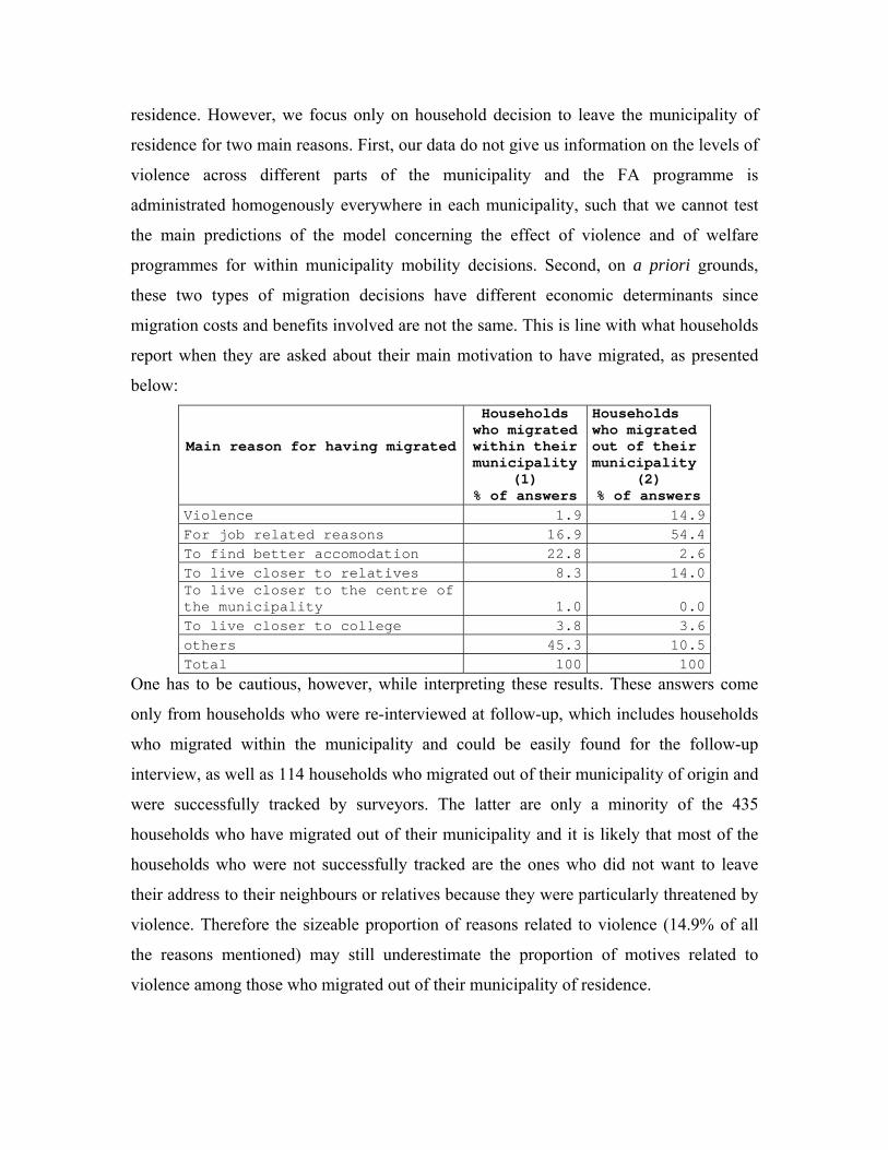
migration costs and benefits involved are not the same. This is line with what households

report when they are asked about their main motivation to have migrated, as presented

below:

Main reason for having migrated

Households who migrated within their municipality

(1) % of answers

Households who migrated out of their municipality

(2) % of answers

Violence 1.9 14.9 For job related reasons 16.9 54.4 To find better accomodation 22.8 2.6 To live closer to relatives 8.3 14.0 To live closer to the centre of the municipality 1.0 0.0 To live closer to college 3.8 3.6 others 45.3 10.5 Total 100 100

One has to be cautious, however, while interpreting these results. These answers come

only from households who were re-interviewed at follow-up, which includes households

who migrated within the municipality and could be easily found for the follow-up

interview, as well as 114 households who migrated out of their municipality of origin and

were successfully tracked by surveyors. The latter are only a minority of the 435

households who have migrated out of their municipality and it is likely that most of the

households who were not successfully tracked are the ones who did not want to leave

their address to their neighbours or relatives because they were particularly threatened by

violence. Therefore the sizeable proportion of reasons related to violence (14.9% of all

the reasons mentioned) may still underestimate the proportion of motives related to

violence among those who migrated out of their municipality of residence.

Therefore, the sample we use in our final analysis comprises 435 households who have

clearly moved out of their municipality of residence -hereafter called “migrants”- as well

as 11177 households who have not, the “non migrants”. We summarise the characteristics

of these two sub-samples in the Dictionary of Variables in Table 1 of Appendix A.

22 Household level variables

As in models of individual migration, we assume that migration costs and benefits

depend strongly on household characteristics. To capture these effects in our regression

framework we will control for a set of demographic variables from the FA survey such as

the number of people in household, its age composition, as well as for education levels,

occupation and age of parents. As shown in Table 1, non-migrant households are

significantly larger (with 6.1 members on average) than migrant households (5.5). Also

non-migrant households report a significantly higher number of children aged 7-17 years

as compared to migrant households. We also capture whether the household head is

single or not since this could motivate the household to migrate in order to join other

relatives or may diminish migration costs. We observe a significantly larger proportion of

single head households among migrants (26%) than among non-migrants (20%). It is also

noticeable that education levels of heads of household are not significantly different

between the two samples, even though spouses in non migrant households are more

frequently not educated (23%) as compared to spouses in migrant households (19%).

However we cannot test a selection model a la Borjas (1987) where migrants choose to

migrate where the returns to human capital are higher since we do not observe the

destination areas of most of migrants or the returns to human capital. However, in line

with migration models based on human capital, we observe that head and spouses in

migrant households are around three years younger on average as compared to non-

migrants.

We also collected information related to the type of social insurance held by each

household. In Colombia, the best type of insurance is offered privately by employers,

which might contribute to attach one employee to his/her job. Table 1 in Appendix shows

that non-migrant households have more frequently unsubsidized health insurance than

migrants (4% versus 2%). Also the proportion of households with a subsidized health

insurance (the second best type of insurance) is significantly larger among non-migrants

(69%) than among migrants (63%). This might be easily explained if good jobs with

good insurance discourage the vulnerable households of our sample to move out of their

municipality of residence. But this could also reflect a selection bias of more risk averse

households who look for safer jobs with better insurance and are not mobile.

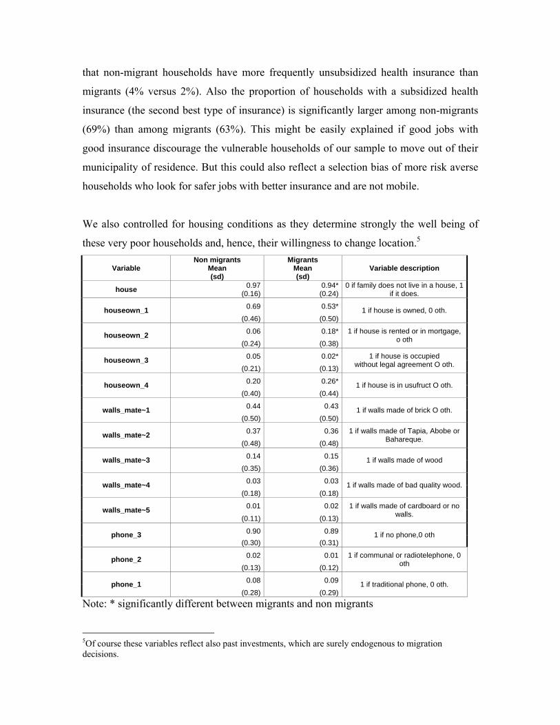
We also controlled for housing conditions as they determine strongly the well being of

these very poor households and, hence, their willingness to change location.5

Variable Non migrants

Mean (sd)

Migrants Mean (sd)

Variable description

house 0.97(0.16)

0.94*(0.24)

0 if family does not live in a house, 1 if it does.

0.69 0.53*houseown_1 (0.46) (0.50)

1 if house is owned, 0 oth.

0.06 0.18*houseown_2 (0.24) (0.38)

1 if house is rented or in mortgage, o oth

0.05 0.02*houseown_3 (0.21) (0.13)

1 if house is occupied without legal agreement O oth.

0.20 0.26*houseown_4 (0.40) (0.44)

1 if house is in usufruct O oth.

0.44 0.43walls_mate~1 (0.50) (0.50)

1 if walls made of brick O oth.

0.37 0.36walls_mate~2 (0.48) (0.48)

1 if walls made of Tapia, Abobe or Bahareque.

0.14 0.15walls_mate~3 (0.35) (0.36)

1 if walls made of wood

0.03 0.03walls_mate~4 (0.18) (0.18)

1 if walls made of bad quality wood.

0.01 0.02walls_mate~5 (0.11) (0.13)

1 if walls made of cardboard or no walls.

0.90 0.89phone_3 (0.30) (0.31)

1 if no phone,0 oth

0.02 0.01phone_2 (0.13) (0.12)

1 if communal or radiotelephone, 0 oth

0.08 0.09phone_1 (0.28) (0.29)

1 if traditional phone, 0 oth.

Note: * significantly different between migrants and non migrants

5Of course these variables reflect also past investments, which are surely endogenous to migration decisions.

The statistics summarised above show that there is a significantly larger proportion of

households living in a house among non migrants (97%) than among migrants (94%).

Furthermore, non-migrants own significantly more frequently their house, as we

understand easily if ownership reflects household intentions to stay. Also non migrant

households occupy their houses more frequently without legal agreement, which may

reflect that similar agreements are difficult to find in destination areas. But migrants rent

or have their house in usufruct more frequently than non migrants.

23 Municipality level variables

The variables used to capture the role played by expected wages predicted by economic

models are standard although we cannot control for expected wages in the destination

area for the reasons already mentioned (see footnote 3). So we control for hourly wages

in rural and urban parts of municipality and occupations of heads and spouses.

Geographic factors may also be important in explaining migration decisions since they

determine returns to agriculture and access to markets. Therefore we included among the

explanatory variables of migration decisions a few characteristics like the altitude of the

municipality of residence and its square. Moreover, to capture better regional imbalances

and other unobserved factors that may affect migration and differ across regions we also

embedded four regional dummy variables into the migration equation, as well as the size

of population living in the center and peripheric parts of the municipalities.6

Moreover, we expect the very poor households in our sample to be sensitive to the

availability of public infrastructure like schools and hospitals that are entered as

additional explanatory variables. We also include the proportion of households with

sewage system or piped water in the municipality of residence, as well as the number of

pharmacies, public centros and puestos as they may reflect the costs of access to these

services. Table 1 shows that migrant households live, before migrating, in villages that

6As the latter also capture dynamic effects linked to agglomeration in specific areas resulting from past migrations, they are potentially endogenous and we need to be cautious while interpreting their effects.

are on average better connected to pipe water or sewage systems, and with more schools,

hospitals and puestos than non migrants.

An important determinant of migration emphasized by the recent literature is the presence

of networks. Although we do not have a direct measure of household networks in our

data, we include proxies for the level of social capital in the village, as well as variables

indicating household participation in collective activities that are likely to affect

migration decisions in complex ways. On one hand social capital may be considered as a

positive amenity that increases the well-being to live in some municipalities and may be

viewed as a social asset that is not easily transferable to another community. On the other

hand, social capital may be correlated to the presence of strong networks, which may

facilitate migration by decreasing its costs, as outlined in the recent literature on

migration.

The FA survey provides us with several sources of information on social capital in the

village. First we computed variables measuring trust in municipalities. This was possible

by using a special module of the survey applied to three leaders in each municipality who

have to grade the level of trust and its evolution during the last five. We averaged the

answers across leaders and added them among the control variables. Second we use a

detailed module of the questionnaire applied to household mothers, which describes

participation of women in political, religious, sport, neighbourhood or other types of

associations. As a proxy for social capital we used the proportion of women involved in

each type of collective activity as well as the proportion of women involved in any of

these groups. Third, we used proxies for social capital coming from the experimental

games that have been implemented in 12 pilot villages. We tried successively several

measures such as the average size of risk sharing groups formed during the games

divided by the number of people in each session, the number of groups (the larger, the

smaller the social capital) or the number of groups divided by the number of people in

each session (see in Appendix F for more details on these games).7

7For efficiency reasons, we added a dummy variable indicating whether a municipality is a pilot for the games or not (in which case no data are available). We hope to be able to extend these games in the future

To assess the impact of violence on migration decisions, different sources of information

from the FA data have been used. The first type of variables comes from the part of the

FA questionnaire on public infrastructure that gives information on the presence of

taskforce desertion and taskforce strike due to violence in any health center (IPS) of the

municipality. Table 1 shows that non-migrants households have been affected by these

events significantly less than migrants. Secondly we use three variables that describe the

perception by the surveyors of some problems linked to violence when they visited the

municipalities. These are three dummy variables equal to one if, respectively, there was a

curfew, if there were some paramilitaries/FARC/or ELN forces, or if there were some

problems related to violence in the municipalities. Table 1 shows that migrants lived in

more violent municipalities before migrating. There was a curfew in the municipality of

12% of non-migrant households, which is a significant lower proportion than among

migrant households (15%). Furthermore, illegal armed groups are more frequently

present in the municipalities of migrant households (73%) than of non-migrant

households (61%). Finally, 65 % of non-migrants households live in a municipality

where there are some problems of public order, which is significantly lower than among

migrant households (78%). The last type of variables measuring the levels of violence

comes from the special module applied to three leaders in each municipality. They

mention whether some displaced households have left and joined the municipality during

the year before the baseline survey. In the hope of getting rid of some measurement errors

in the answers, we use the average of the answers reported by the leaders in each

municipality. Table 1 shows that, on average, almost twice as much displaced households

have left the municipalities of residence of migrants as compared to non migrants.

3 Results

We report the determinants of household decision to migrate out of the municipality of

residence between the baseline and follow-up surveys after discussing several

to the 122 municipalities, which will give us more variation in social capital and allow us to assess better its effect.

specifications we used to measure the effects of the programme and its interaction with

the level of violence in the municipalities. In the last subsection, we address whether the

incidence of violence modifies migration incentives of households with different

characteristics.

31 Main results

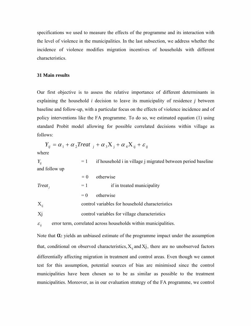
Our first objective is to assess the relative importance of different determinants in

explaining the household i decision to leave its municipality of residence j between

baseline and follow-up, with a particular focus on the effects of violence incidence and of

policy interventions like the FA programme. To do so, we estimated equation (1) using

standard Probit model allowing for possible correlated decisions within village as

follows:

ijjij TreatY εαααα ++++= ij4j321 XX where

ijY = 1 if household i in village j migrated between period baseline and follow up

= 0 otherwise

jTreat = 1 if in treated municipality

= 0 otherwise

ijX control variables for household characteristics

Xj control variables for village characteristics

ijε error term, correlated across households within municipalities.

Note that α2 yields an unbiased estimate of the programme impact under the assumption

that, conditional on observed characteristics, ijX and Xj, there are no unobserved factors

differentially affecting migration in treatment and control areas. Even though we cannot

test for this assumption, potential sources of bias are minimised since the control

municipalities have been chosen so to be as similar as possible to the treatment

municipalities. Moreover, as in our evaluation strategy of the FA programme, we control

for many observable variables, both at the municipality and household level (see

Attanasio et al, 2005).

The main results we discuss below are presented in Table 2 in Appendix. In the first

specification presented in column (1) we used as many regressors as municipality

variables as we had. Since the effects associated to the public infrastructure variables are

not easy to interpret, we wanted to check for the robustness of our results when we drop

these regressors, as presented in column (2). We also test for the robustness of our results

when we include more control variables to capture better job related motives: in column

(3), we add more education levels of the household heads and spouses, and in column (4),

their occupations. Column (5) includes an additional variable “group” measuring the

average participation of women in collective activities to control for the social capital in

the village. All these specifications and their results are discussed below.

We find that geographic factors make some areas more attractive than others. The

households living in the Oriental area and in the Pacific area have a lower probability to

migrate out of their municipality as compared to households living in the Atlantic areas,

the missing category. Also the altitude of the municipality increases the probability to

migrate out of the municipality, which might be explained by lower returns to agriculture

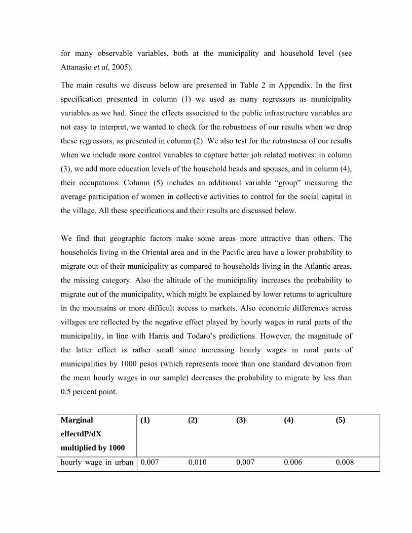
in the mountains or more difficult access to markets. Also economic differences across

villages are reflected by the negative effect played by hourly wages in rural parts of the

municipality, in line with Harris and Todaro’s predictions. However, the magnitude of

the latter effect is rather small since increasing hourly wages in rural parts of

municipalities by 1000 pesos (which represents more than one standard deviation from

the mean hourly wages in our sample) decreases the probability to migrate by less than

0.5 percent point.

Marginal

effectdP/dX

multiplied by 1000

(1) (2) (3) (4) (5)

hourly wage in urban 0.007 0.010 0.007 0.006 0.008

part of municipality

(0.010) (0.008) (0.010) (0.008) (0.010)

hourly wage in rural

part of municipality

-0.005 -0.004 -0.004 -0.003 -0.005

(0.002)** (0.002) (0.002)** (0.002) (0.002)**

Notes : Robust standard errors in parentheses * significant at 10%; ** significant at 5%; *** significant at 1%

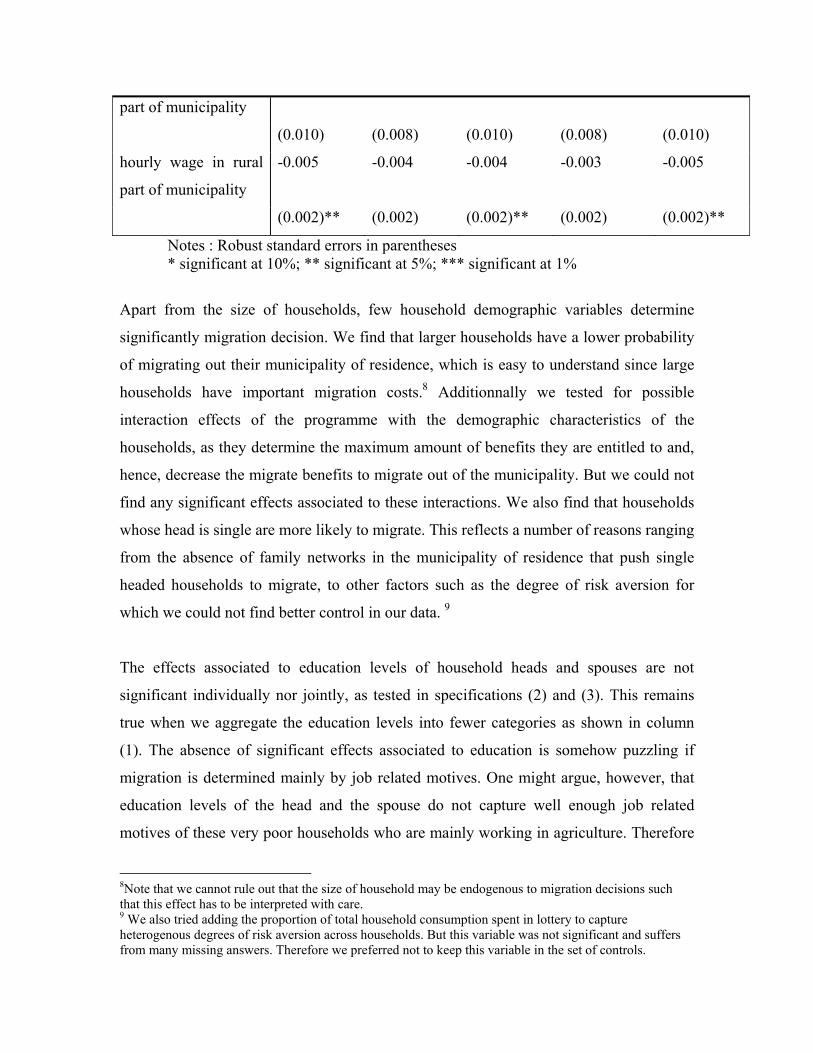
Apart from the size of households, few household demographic variables determine

significantly migration decision. We find that larger households have a lower probability

of migrating out their municipality of residence, which is easy to understand since large

households have important migration costs.8 Additionnally we tested for possible

interaction effects of the programme with the demographic characteristics of the

households, as they determine the maximum amount of benefits they are entitled to and,

hence, decrease the migrate benefits to migrate out of the municipality. But we could not

find any significant effects associated to these interactions. We also find that households

whose head is single are more likely to migrate. This reflects a number of reasons ranging

from the absence of family networks in the municipality of residence that push single

headed households to migrate, to other factors such as the degree of risk aversion for

which we could not find better control in our data. 9

The effects associated to education levels of household heads and spouses are not

significant individually nor jointly, as tested in specifications (2) and (3). This remains

true when we aggregate the education levels into fewer categories as shown in column

(1). The absence of significant effects associated to education is somehow puzzling if

migration is determined mainly by job related motives. One might argue, however, that

education levels of the head and the spouse do not capture well enough job related

motives of these very poor households who are mainly working in agriculture. Therefore

8Note that we cannot rule out that the size of household may be endogenous to migration decisions such that this effect has to be interpreted with care. 9 We also tried adding the proportion of total household consumption spent in lottery to capture heterogenous degrees of risk aversion across households. But this variable was not significant and suffers from many missing answers. Therefore we preferred not to keep this variable in the set of controls.

we added some control variables for occupations of heads and spouses in specification

(4). We find that if the head is working the household probability to migrate is higher,

and that being a self-employed worker, an employer or employed dimishes the

probability to migrate, as we can easily explain with job related motives. We cannot,

however, overinterpret these findings since occupations of heads and spouses just before

migrating are surely endogenous to household migration decisions. Therefore we present

the results with these additional controls for occupation separately from the others in

column (4).

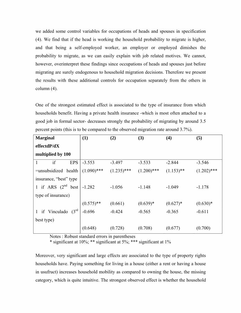
One of the strongest estimated effect is associated to the type of insurance from which

households benefit. Having a private health insurance -which is most often attached to a

good job in formal sector- decreases strongly the probability of migrating by around 3.5

percent points (this is to be compared to the observed migration rate around 3.7%).

Marginal

effectdP/dX

multiplied by 100

(1) (2) (3) (4) (5)

1 if EPS

=unsubsidized health

insurance, “best” type

-3.553

(1.090)***

-3.497

(1.235)***

-3.533

(1.200)***

-2.844

(1.153)**

-3.546

(1.202)***

1 if ARS (2nd best

type of insurance)

-1.282 -1.056 -1.148 -1.049 -1.178

(0.575)** (0.661) (0.639)* (0.627)* (0.630)*

1 if Vinculado (3rd

best type)

-0.696 -0.424 -0.565 -0.365 -0.611

(0.648) (0.728) (0.708) (0.677) (0.700)

Notes : Robust standard errors in parentheses * significant at 10%; ** significant at 5%; *** significant at 1%

Moreover, very significant and large effects are associated to the type of property rights

households have. Paying something for living in a house (either a rent or having a house

in usufruct) increases household mobility as compared to owning the house, the missing

category, which is quite intuitive. The strongest observed effect is whether the household

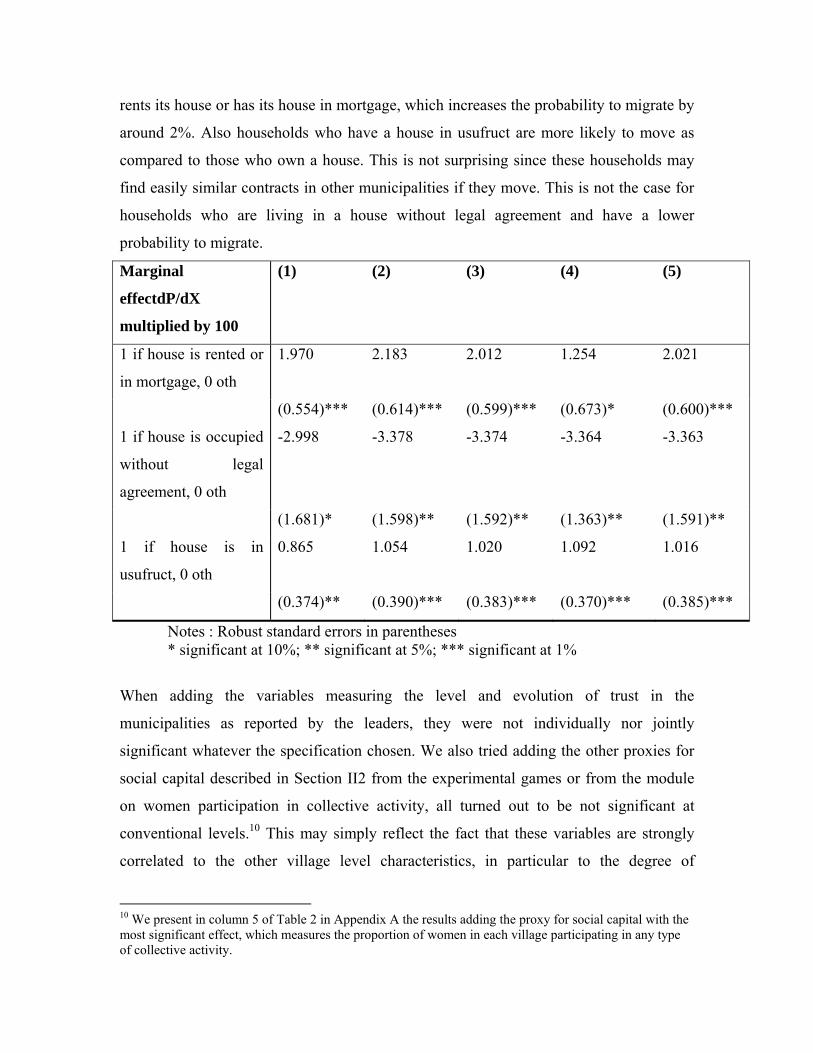
rents its house or has its house in mortgage, which increases the probability to migrate by

around 2%. Also households who have a house in usufruct are more likely to move as

compared to those who own a house. This is not surprising since these households may

find easily similar contracts in other municipalities if they move. This is not the case for

households who are living in a house without legal agreement and have a lower

probability to migrate.

Marginal

effectdP/dX

multiplied by 100

(1) (2) (3) (4) (5)

1 if house is rented or

in mortgage, 0 oth

1.970 2.183 2.012 1.254 2.021

(0.554)*** (0.614)*** (0.599)*** (0.673)* (0.600)***

1 if house is occupied

without legal

agreement, 0 oth

-2.998 -3.378 -3.374 -3.364 -3.363

(1.681)* (1.598)** (1.592)** (1.363)** (1.591)**

1 if house is in

usufruct, 0 oth

0.865 1.054 1.020 1.092 1.016

(0.374)** (0.390)*** (0.383)*** (0.370)*** (0.385)***

Notes : Robust standard errors in parentheses * significant at 10%; ** significant at 5%; *** significant at 1%

When adding the variables measuring the level and evolution of trust in the

municipalities as reported by the leaders, they were not individually nor jointly

significant whatever the specification chosen. We also tried adding the other proxies for

social capital described in Section II2 from the experimental games or from the module

on women participation in collective activity, all turned out to be not significant at

conventional levels.10 This may simply reflect the fact that these variables are strongly

correlated to the other village level characteristics, in particular to the degree of

10 We present in column 5 of Table 2 in Appendix A the results adding the proxy for social capital with the most significant effect, which measures the proportion of women in each village participating in any type of collective activity.

violence.11 Moreover, we entered the household level variables measuring mother’s

participation in collective activities, which were not significant either. Hence we chose

not to report them in the final results.

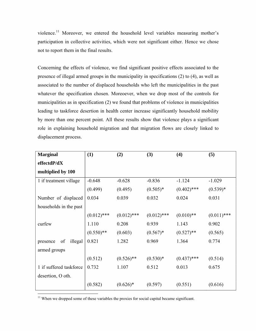
Concerning the effects of violence, we find significant positive effects associated to the

presence of illegal armed groups in the municipality in specifications (2) to (4), as well as

associated to the number of displaced households who left the municipalities in the past

whatever the specification chosen. Moreoever, when we drop most of the controls for

municipalities as in specification (2) we found that problems of violence in municipalities

leading to taskforce desertion in health center increase significantly household mobility

by more than one percent point. All these results show that violence plays a significant

role in explaining household migration and that migration flows are closely linked to

displacement process.

Marginal

effectdP/dX

multiplied by 100

(1) (2) (3) (4) (5)

1 if treatment village -0.648 -0.628 -0.836 -1.124 -1.029

(0.499) (0.495) (0.505)* (0.402)*** (0.539)*

Number of displaced

households in the past

0.034 0.039 0.032 0.024 0.031

(0.012)*** (0.012)*** (0.012)*** (0.010)** (0.011)***

curfew 1.110 0.208 0.939 1.143 0.902

(0.550)** (0.603) (0.567)* (0.527)** (0.565)

presence of illegal

armed groups

0.821 1.282 0.969 1.364 0.774

(0.512) (0.526)** (0.530)* (0.437)*** (0.514)

1 if suffered taskforce

desertion, O oth.

0.732 1.107 0.512 0.013 0.675

(0.582) (0.626)* (0.597) (0.551) (0.616)

11 When we dropped some of these variables the proxies for social capital became significant.

Notes : Robust standard errors in parentheses * significant at 10%; ** significant at 5%; *** significant at 1%

Turning now to the effect of the programme, it is only significant when we add more

control for municipality infrastructure and for education variables, as in columns (3) to

(5). This effect is not negligible since receiving the programme decreases by around

probability to migrate as compared to the observed migration rate equal to 3.73 %.

Interestingly, the magnitude of this negative effect associated to the programme is

comparable to the magnitude of the positive effect associated to the level of violence in

the municipality as measured by the coefficient associated to the presence of illegal

armed groups. This would suggest that the programme contributes to stabilise the

situation in some municipalities by mitigating migration flows due to high incidence of

violence.

32 Robustness checks

We were also worried that the lack of significance of the programme effect in some

specifications like in columns (1) and (2) could be driven by some misspecification of the

programme effect. So far, we captured the effect of the programme by a dummy variable

indicating whether the municipality of residence of a household receives the programme

or not. However, in order to assess the programme’s effect as accurately as possible, we

also exploited an interesting feature of the implementation of the programme that started

at different dates in different municipalities. As a consequence some municipalities have

received more payments at follow up. We captured this “intensity” effect of the

programme with the variable “number of payments” and estimated the following

equation (2):

ijjij xpoY εαααα ++++= ij4j321 XXE

where the variable jxpoE measures the number of payments received in municipality j at

follow up survey.

The results shown in Table 3 in Appendix show that the intensity effect of the

programme is positive and significant at 10 % level (and, as expected, negative) when we

add more control variables either at municipality level as in column (1) or at household

level in column (3).12 We find robust results concerning the main effects we already

discussed.

Moreover we could not exclude that the effect of the programme on migration might play

beyond its intensity effect like a “fixed” effect, for example if it has positive externalities

in the municipalities that discourage households to migrate. Therefore we tried another

specification by allowing for the programme to affect the probability to migrate

separately from the number of payments received. The estimated model became:

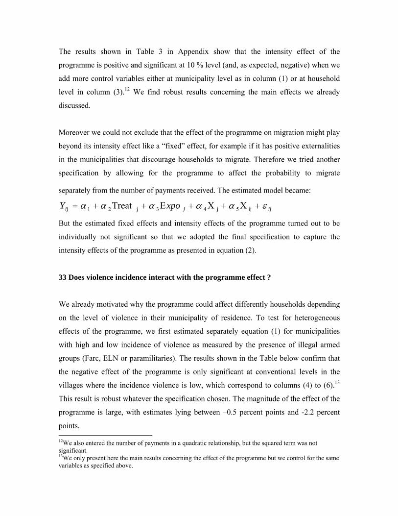
ijjij xpoY εααααα +++++= ij5j43j21 XXE Treat

But the estimated fixed effects and intensity effects of the programme turned out to be

individually not significant so that we adopted the final specification to capture the

intensity effects of the programme as presented in equation (2).

33 Does violence incidence interact with the programme effect ?

We already motivated why the programme could affect differently households depending

on the level of violence in their municipality of residence. To test for heterogeneous

effects of the programme, we first estimated separately equation (1) for municipalities

with high and low incidence of violence as measured by the presence of illegal armed

groups (Farc, ELN or paramilitaries). The results shown in the Table below confirm that

the negative effect of the programme is only significant at conventional levels in the

villages where the incidence violence is low, which correspond to columns (4) to (6).13

This result is robust whatever the specification chosen. The magnitude of the effect of the

programme is large, with estimates lying between –0.5 percent points and -2.2 percent

points. 12We also entered the number of payments in a quadratic relationship, but the squared term was not significant. 13We only present here the main results concerning the effect of the programme but we control for the same variables as specified above.

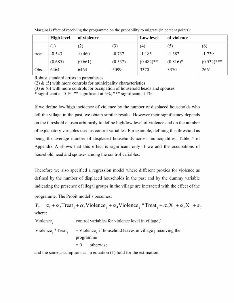
Marginal effect of receiving the programme on the probability to migrate (in percent points):

High level of violence Low level of violence

(1) (2) (3) (4) (5) (6)

treat -0.543 -0.460 -0.737 -1.185 -1.382 -1.739

(0.685) (0.661) (0.537) (0.482)** (0.816)* (0.532)***

Obs. 6464 6464 5099 3370 3370 2661

Robust standard errors in parentheses. (2) & (5) with more controls for municipality characteristics (3) & (6) with more controls for occupation of household heads and spouses * significant at 10%; ** significant at 5%; *** significant at 1%

If we define low/high incidence of violence by the number of displaced households who

left the village in the past, we obtain similar results. However their significancy depends

on the threshold chosen arbitrarily to define high/low level of violence and on the number

of explanatory variables used as control variables. For example, defining this threshold as

being the average number of displaced households across municipalities, Table 4 of

Appendix A shows that this effect is significant only if we add the occupations of

household head and spouses among the control variables.

Therefore we also specified a regression model where different proxies for violence as

defined by the number of displaced households in the past and by the dummy variable

indicating the presence of illegal groups in the village are interacted with the effect of the

programme. The Probit model’s becomes:

ijjjijY εαααααα ++++++= ij6j5j43j21 XXTreat*ViolenceViolence Treatwhere:

jViolence control variables for violence level in village j

jTreat*Violence j = jViolence if household leaves in village j receiving the programme

= 0 otherwise

and the same assumptions as in equation (1) hold for the estimation.

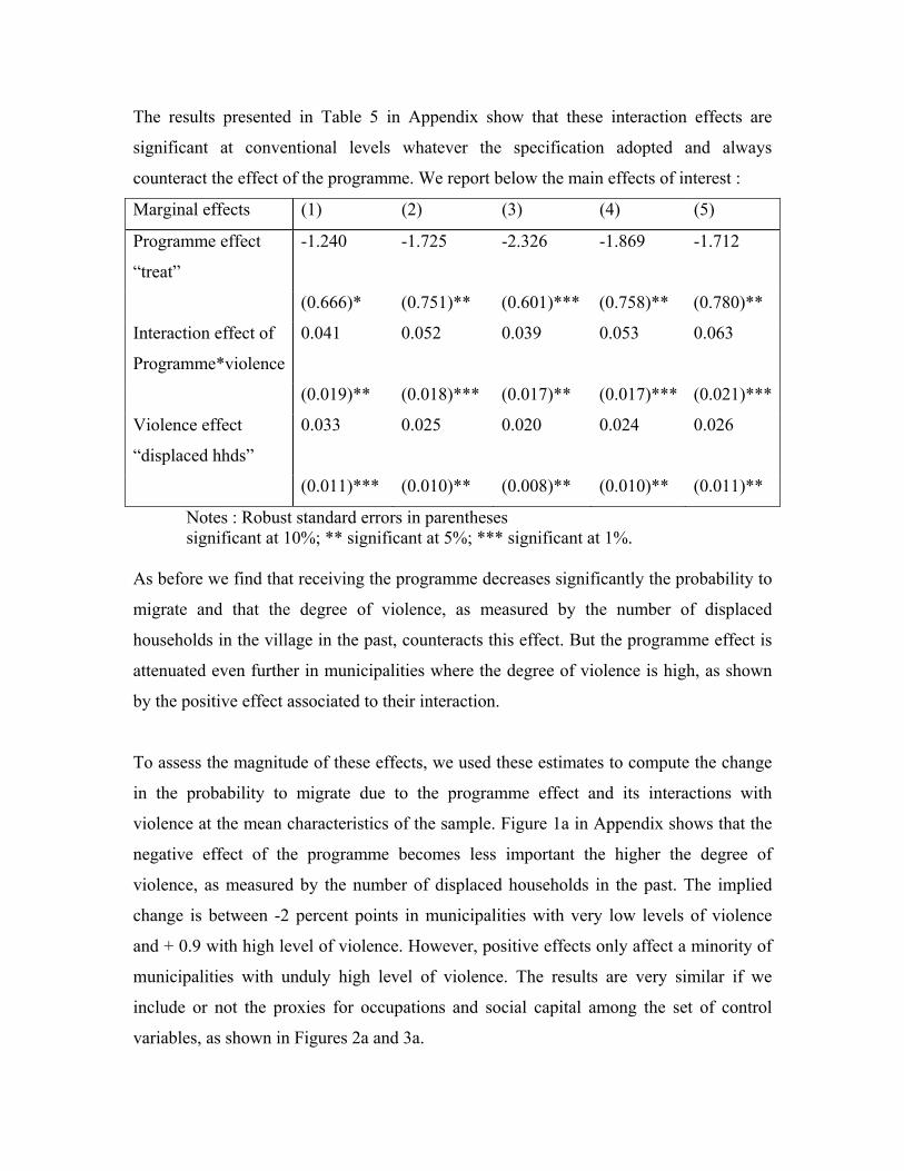
The results presented in Table 5 in Appendix show that these interaction effects are

significant at conventional levels whatever the specification adopted and always

counteract the effect of the programme. We report below the main effects of interest :

Marginal effects (1) (2) (3) (4) (5)

Programme effect

“treat”

-1.240 -1.725 -2.326 -1.869 -1.712

(0.666)* (0.751)** (0.601)*** (0.758)** (0.780)**

Interaction effect of

Programme*violence

0.041 0.052 0.039 0.053 0.063

(0.019)** (0.018)*** (0.017)** (0.017)*** (0.021)***

Violence effect

“displaced hhds”

0.033 0.025 0.020 0.024 0.026

(0.011)*** (0.010)** (0.008)** (0.010)** (0.011)**

Notes : Robust standard errors in parentheses significant at 10%; ** significant at 5%; *** significant at 1%.

As before we find that receiving the programme decreases significantly the probability to

migrate and that the degree of violence, as measured by the number of displaced

households in the village in the past, counteracts this effect. But the programme effect is

attenuated even further in municipalities where the degree of violence is high, as shown

by the positive effect associated to their interaction.

To assess the magnitude of these effects, we used these estimates to compute the change

in the probability to migrate due to the programme effect and its interactions with

violence at the mean characteristics of the sample. Figure 1a in Appendix shows that the

negative effect of the programme becomes less important the higher the degree of

violence, as measured by the number of displaced households in the past. The implied

change is between -2 percent points in municipalities with very low levels of violence

and + 0.9 with high level of violence. However, positive effects only affect a minority of

municipalities with unduly high level of violence. The results are very similar if we

include or not the proxies for occupations and social capital among the set of control

variables, as shown in Figures 2a and 3a.

We then performed the same computations but by adding to the programme effect and its

interactions with violence the direct effect played by violence incidence in our migration

equation. Figures 1b to 3b show that for the big majority of treated villages the negative

effect of the programme more than offsets the effect of violence. However, the total

effect becomes positive when more than 20 households have left the village in the past,

which corresponds to violence levels observed in the 10% most violent municipalities of

our sample.

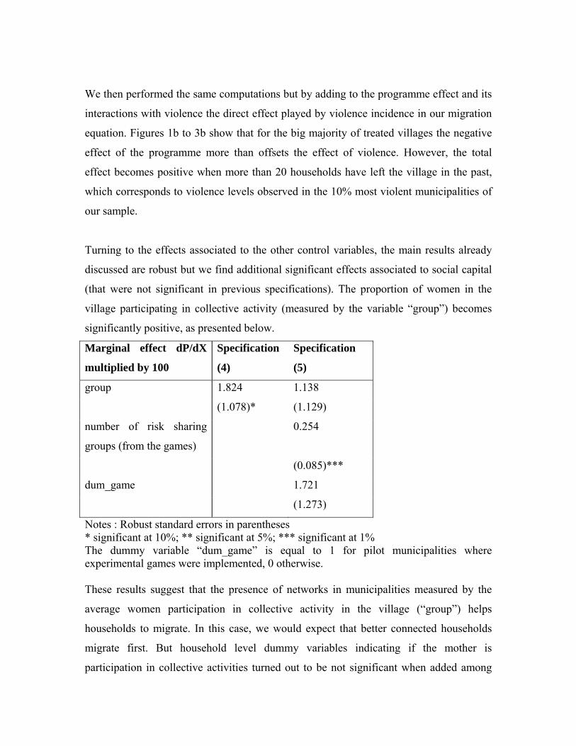
Turning to the effects associated to the other control variables, the main results already

discussed are robust but we find additional significant effects associated to social capital

(that were not significant in previous specifications). The proportion of women in the

village participating in collective activity (measured by the variable “group”) becomes

significantly positive, as presented below.

Marginal effect dP/dX

multiplied by 100

Specification

(4)

Specification

(5)

group 1.824 1.138

(1.078)* (1.129)

number of risk sharing

groups (from the games)

0.254

(0.085)***

dum_game 1.721

(1.273)

Notes : Robust standard errors in parentheses * significant at 10%; ** significant at 5%; *** significant at 1% The dummy variable “dum_game” is equal to 1 for pilot municipalities where experimental games were implemented, 0 otherwise. These results suggest that the presence of networks in municipalities measured by the

average women participation in collective activity in the village (“group”) helps

households to migrate. In this case, we would expect that better connected households

migrate first. But household level dummy variables indicating if the mother is

participation in collective activities turned out to be not significant when added among

the control variables.14 Moreover, we find positive effects associated to the number of

groups formed during experimental games, contrary to what we would expect if more

groups is correlated to less social capital in the village. However we could not confirm

these results by using other proxies for social capital resulting from the games, which

turn out to be not significant; and the same variable measuring the number of groups turn

out to be not significant while using different specifications (as for example in Table 2).

To test for the robustness of our results concerning social capital, we would need more

variation across villages in the proxies for social capital resulting from the games, which

we hope to obtain in the future by extending the games to all municipalities surveyed for

the evaluation.

We were also worried that the programme may have a stronger impact on migration

decisions in municipalities characterised by high levels of social capital. Therefore we

added some control variables for possible interaction effects of the programme with

social capital. But these additional interactions turned out to be not significant, so that we

do not present them in our results.

34 Does violence incidence modify household incentives to migrate ?

We also argued in the motivations of the model that the level of violence in the

municipalities could affect differently household migration incentives depending on their

characteristics. This is for example the case when households are displaced by violence,

as outlined by Ibanez and Velez (2005). To address this issue, we interacted the proxies

for violence with other household characteristics. All results are presented in Table 6 in

the Appendix.

As shown in Table 6 of Appendix A, we do not find any significant effects associated to

the interactions of violence with socio-economic characteristics like education levels of

the head and the spouse, living in an isolated rural part of the municipality or working in

agriculture, as we would have expected if these households were more threatened by

14Hence we do not present the effects associated to these controls.

violence. We also did not find evidence of significant interaction effects of violence

incidence with household participation in collective activities, contrary to one would

expect if households with strong social connections were strategically targeted by illegal

armed groups.15

Instead, we found that households with larger size, less children, and whose head

(spouse) is older (younger) respond more strongly to the level of violence by leaving their

municipality of residence. This suggests that large households who would not otherwise

have migrated due to high migration costs may be pushed to migrate by high incidence of

violence. Hence migration decisions of households in our sample respond differently to

violence from what we would expect if mobility was forced. Another explanation for

these findings is simply that the households in our sample are the most deprived

households living in rural areas of Colombia. This is maybe not too surprising if illegal

armed groups did not particularly target according to their socio economic statut in their

strategy to destabilise rural areas.

III The consequences of mobility and displacement.

In the previous section we studied a data set that included households that were

interviewed in 2002, some of which had left the municipality of residence in 2003 and

characterized the differences between the households that left and those who stayed.

While a considerable number of the movers moved because of violence16, many others

moved for other reasons. For this reason, we think of the analysis of the previous section

as relevant for migration in general, rather than displacement in particular. In other

words, our movers include both displaced and economic migrants. Moreover, probably in

many cases, the two motives actually overlap. It is this aspect that differentiates our

contribution from other studies existing in the literature. In this section, we make our

analysis comparable and complementary to the pre-existing evidence in two ways. First,

15The latter results are not presented since they are not significant. 16 This cannot be checked for the households that we are unable to track between surveys.

we present a descriptive analysis of the households in the FA dataset that moved and

were successfully tracked. The analysis is only descriptive because of the small sample

size. Second, we combine the information in our dataset with another dataset that

contains information on displaced individuals, as traditionally defined, interviewed in

receiving municipalities, typically big cities. This combination of datasets allows us to

compare the FA dataset households with displaced households and check whether they

are very different and differentiate and characterize further the two inter-related

phenomena we are studying: migration and displacement.

Among the households who have left their municipality of residence between the baseline

and follow up, 113 households were successfully tracked by the interviewers and

surveyed in their new location. Section 31 presents what we learn on the migration

process and its economic consequences from the special part of the survey that was

applied to these households. However, describing the reasons why these households

chose to migrate, we already observed that this selected sample of migrants does not

represent the population of displaced households. In order to complete our information on

forced migration, Section 32 presents results from a specific survey involving displaced

households in their areas of relocation. To assess their relative poverty level, Section 33

compares them to the very poor households surveyed for the evaluation of the FA welfare

programme, while Section 34 compares them to the households that have chosen to

migrate.

III 1 consequences of household migration

11 Reasons for migration

Amongst the 113 successfully tracked households, only 16 households report that they

have migrated because of movements of illegal armed groups in the municipality. 13

households have moved because they had been thinking about it for a long time.

However, most of the households (83 of them) are not explicit about the reason why they

moved, and one household does not answer. This is at this stage not very informative

since there are many reasons why the households who moved due to the violence might

be reluctant to give information about it. Moreover we mentioned already that there

might be a selection bias of the sample since households who migrated because of

violence may be more likely not to have been successfully tracked and, hence, are not

part of these answers.

The households also explain why they chose the destination municipality where they are

interviewed (the answers are not exclusive). The main reasons are that they had better

opportunities to work (53 answers) or that some friends or relatives living in the

municipality advised them to move in (32 answers). 10 households chose to live in

municipalities close to their origin municipalities, others in municipalities that provide

them with better services for the education of their children (6 answers) or better health

services (2 answers) and 4 households chose to live in safer municipalities. Accordingly

it seems that none of them have been relocated into the destination municipality without

choosing it, even though some of them have moved because of the increasing level of

violence in their origin municipalities.

12 Intentions to move again in the future

Most of households who are tracked by interviewers after migration do not consider

staying in the destination area for ever. 16 households intend to stay in the new location

until they can return to their origin municipality, while 40 intend to stay permanently and

32 do not know. The remaining households intend to stay in the destination municipality

for 2 years on average, with an expected duration lying between 1 and 4.3 years.

Surveyors also ask households whether they wish to leave the destination municipality in

the future: among 47 positive answers, 30 households would like to move to their origin

municipalities and 17 to another municipality. None of them considers migrating to a

foreign country. When asked about their motivations, most of these households want to

return to their municipality of origin (19 answers), or to find better job opportunities (18

answers). Others want to find a better quality of life (3 answers), or good education

services (4 answers) or good health services (4 answers). Only 6 households mention the

problems related to violence as being the main reason explaining why they consider

migrating again in the future.

The importance of temporary migration emphasizes the role played by uncertainties in

the migration process. This is also confirmed by the importance of networks in explaining

migration. 90% of the sample knew at least one family in the destination municipality

before leaving, and, on average, each household knew 6.5 families. 12 households moved

simultaneously with other relatives.

13 Migration benefits and costs

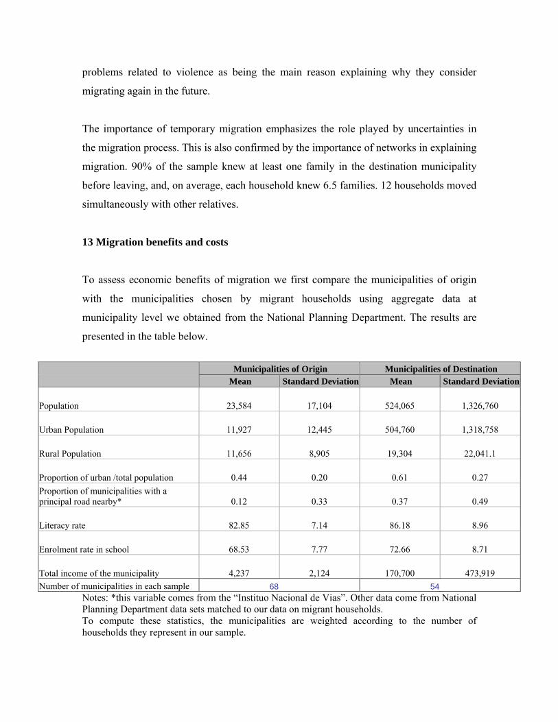
To assess economic benefits of migration we first compare the municipalities of origin

with the municipalities chosen by migrant households using aggregate data at

municipality level we obtained from the National Planning Department. The results are

presented in the table below.

Notes: *this variable comes from the “Instituo Nacional de Vias”. Other data come from National Planning Department data sets matched to our data on migrant households. To compute these statistics, the municipalities are weighted according to the number of households they represent in our sample.

Municipalities of Origin Municipalities of Destination Mean Standard Deviation Mean Standard Deviation

Population 23,584 17,104 524,065 1,326,760

Urban Population 11,927 12,445 504,760 1,318,758

Rural Population 11,656 8,905 19,304 22,041.1

Proportion of urban /total population 0.44 0.20 0.61 0.27 Proportion of municipalities with a principal road nearby* 0.12 0.33 0.37 0.49

Literacy rate 82.85 7.14 86.18 8.96

Enrolment rate in school 68.53 7.77 72.66 8.71

Total income of the municipality 4,237 2,124 170,700 473,919 Number of municipalities in each sample 68 54

Destination municipalities are much larger than origin municipalities, more urbanised,

richer and more developed as measured by the fact that they are more often close to a

main road, they have a higher literacy rate and children are more often enrolled in

schools.

More directly, migrant households are asked about the economic consequences of

migration. Expected benefits of migration are mainly job related: 88 households think

that their job opportunities are better in destination than in origin municipality, while 25

households do not think it is the case. Moreover, 48 household heads changed job after

migration and 9 do not work, while 56 household heads have a similar job as the one they

had before migrating.

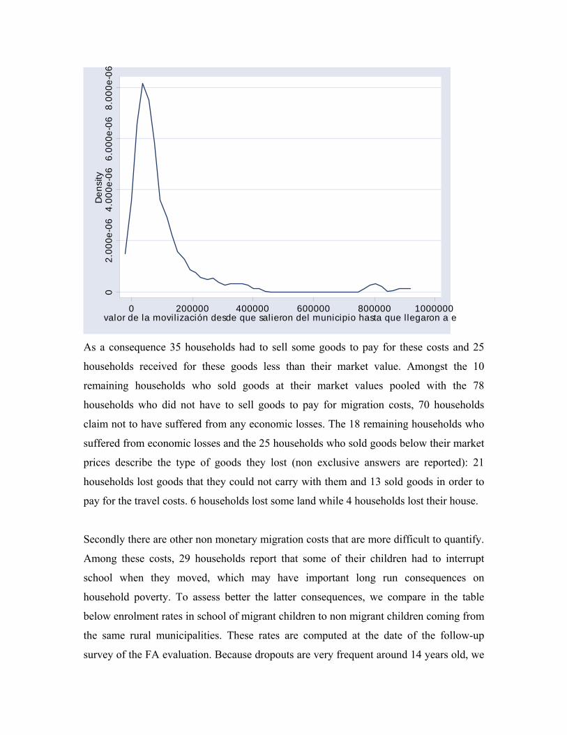
However migration costs are also non negligible for these very poor households and have

many dimensions. Firstly, monetary migration costs are sizeable, as reported by migrants

to the interviewers. The distribution of migration costs is represented in the figure above.

The median costs are around 50.000 pesos and the mean around 103.037 pesos. These

figures represent respectively 21% and 43% of the average monthly total income in the

treated municipalities (according to the baseline report). To finance these costs, 2/3 of

households used their own funds, 1/3 was helped by friends or relative and none relied on

any kind of credit or loan. This shows that the poor households interviewed for FA have

no access to credit markets to finance their migration, even though these costs represent a

sizeable part of their income.

02.

000e

-06

4.00

0e-0

66.

000e

-06

8.00

0e-0

6D

ensi

ty

0 200000 400000 600000 800000 1000000valor de la movil ización desde que salieron del municipio hasta que llegaron a e

As a consequence 35 households had to sell some goods to pay for these costs and 25

households received for these goods less than their market value. Amongst the 10

remaining households who sold goods at their market values pooled with the 78

households who did not have to sell goods to pay for migration costs, 70 households

claim not to have suffered from any economic losses. The 18 remaining households who

suffered from economic losses and the 25 households who sold goods below their market

prices describe the type of goods they lost (non exclusive answers are reported): 21

households lost goods that they could not carry with them and 13 sold goods in order to

pay for the travel costs. 6 households lost some land while 4 households lost their house.

Secondly there are other non monetary migration costs that are more difficult to quantify.

Among these costs, 29 households report that some of their children had to interrupt

school when they moved, which may have important long run consequences on

household poverty. To assess better the latter consequences, we compare in the table

below enrolment rates in school of migrant children to non migrant children coming from

the same rural municipalities. These rates are computed at the date of the follow-up

survey of the FA evaluation. Because dropouts are very frequent around 14 years old, we

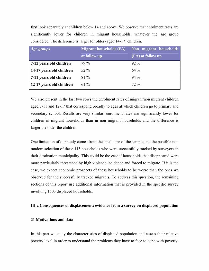
first look separately at children below 14 and above. We observe that enrolment rates are

significantly lower for children in migrant households, whatever the age group

considered. The difference is larger for older (aged 14-17) children.

Age groups Migrant households (FA)

at follow up

Non migrant households

(FA) at follow up

7-13 years old children 79 % 92 %

14-17 years old children 52 % 64 %

7-11 years old children 81 % 94 %

12-17 years old children 61 % 72 %

We also present in the last two rows the enrolment rates of migrant/non migrant children

aged 7-11 and 12-17 that correspond broadly to ages at which children go to primary and

secondary school. Results are very similar: enrolment rates are significantly lower for

children in migrant households than in non migrant households and the difference is

larger the older the children.

One limitation of our study comes from the small size of the sample and the possible non

random selection of these 113 households who were successfully tracked by surveyors in

their destination municipality. This could be the case if households that disappeared were

more particularly threatened by high violence incidence and forced to migrate. If it is the

case, we expect economic prospects of these households to be worse than the ones we

observed for the successfully tracked migrants. To address this question, the remaining

sections of this report use additional information that is provided in the specific survey

involving 1503 displaced households.

III 2 Consequences of displacement: evidence from a survey on displaced population

21 Motivations and data

In this part we study the characteristics of displaced population and assess their relative

poverty level in order to understand the problems they have to face to cope with poverty.

This is an important question for policy makers who have to decide whether they should

target them with specific anti-poverty programmes. To our knowledge, this question has

been largely ignored even in past evaluations of some specific programmes targeted to

displaced households that exclusively focused on displaced households. The main

problem is to find good data that permit to compare displaced households with non-

displaced ones.17

We use as a benchmark the survey designed for the evaluation of FA since it provides us

with very detailed data both at municipality and household levels on the poorest of the

poor households living in rural areas of Colombia. We also exploit another survey about

living conditions of the population displaced by the violence in Colombia that included a

questionnaire very similar to that of the FA data. In 41 municipalities randomly selected

among destination areas of displaced households, 1503 households were surveyed in

March 2003 about their living and food security conditions, their food acquisition, as well

as the coping mechanisms they used after displacement. Using these data, a first report

was released in June 2003 by the WFP on the “Vulnerability to food insecurity of the

population displaced by violence in Colombia”. This report shows that displaced

households suffer from major deficiencies in nutritional requirements and are affected by

serious food insecurity conditions, mainly due to their inability to generating enough

income to allow for the provision of their food needs. The WFP report also compares the

situation of the population displaced by the violence with the poorest population in urban

zones and finds that the former are worse-off. Even though this report is an interesting

step to describe the food insecurity of displaced households in destination areas, no

attempt has been made to compare displaced households with poor households coming

from the same rural areas, which is our main objective. Moreover, the very rich FA data

set on non displaced populations improves the precision of our estimates and makes our

sample at least as informative as that in Ibañez and Velez (2005).

17 Most of existing surveys are exclusively focused on displaced households given the very specific methods required to survey them.

Based on the results of the previous section, we are also quite confident that displacement

rates and migration rates are intrinsically linked. The results presented in Section II

suggest that a sizeable part of migration is determined by the high level of violence in the

municipalities. To increase our confidence, we compared the magnitudes of migration

flows out of the municipalities surveyed for the evaluation of FA with displacement rates

we computed using the data on displaced population from the Red de Solidaridad. The

comparison was made for the same period around the baseline survey and for the same

122 municipalities. The results presented in Appendix B suggest that migration rates are

larger than displacement rates, but that a non-negligible part of them (1/4 on average) is

due to displacement.

However, the displaced households may not be representative of the households who

migrated out of the poor municipalities surveyed for FA. This is why the last section of

the report will describe in details the living conditions of households after displacement

and compare, as much as the data allow us to do so, the displaced households with the

migrant households surveyed for the FA programme. One shortcoming is that the survey

on displaced populations has selected randomly municipalities in urban zones where the

displaced populations are concentrated, whereas the Baseline of Familias en Accion

survey was implemented in rural zones. However, since we want to compare displaced

households -who come mainly from rural areas- to poor households who are living in the

same areas as where they used to live before displacement, this is not a big concern.

Therefore we kept in the “restricted sample” only the 1225 displaced households who

used to live in areas where some municipalities have also been selected for the Familias

en Accion programme18.

22 Migration history of displaced households

Where do displaced households come from? As shown in Table 1, the displaced

households in our sample are coming from all areas of Colombia affected by the conflict

18 Hence, when we compare displaced and non displaced households, we exclude 278 displaced households for whom we could not find a comparison group.

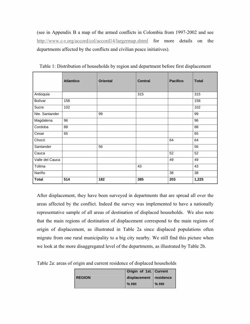
(see in Appendix B a map of the armed conflicts in Colombia from 1997-2002 and see

http://www.c-r.org/accord/col/accord14/largermap.shtml for more details on the

departments affected by the conflicts and civilian peace initiatives).

Table 1: Distribution of households by region and department before first displacement

Atlantico Oriental Central Pacifico Total

Antioquia 315 315

Bolívar 158 158

Sucre 102 102

Nte. Santander 99 99

Magdalena 96 96

Cordoba 88 88

Cesar 65 65

Chocó 64 64

Santander 56 56

Cauca 52 52

Valle del Cauca 49 49

Tolima 43 43

Nariño 38 38

Total 514 182 385 203 1,225

After displacement, they have been surveyed in departments that are spread all over the

areas affected by the conflict. Indeed the survey was implemented to have a nationally

representative sample of all areas of destination of displaced households. We also note

that the main regions of destination of displacement correspond to the main regions of

origin of displacement, as illustrated in Table 2a since displaced populations often

migrate from one rural municipality to a big city nearby. We still find this picture when

we look at the more disaggregated level of the departments, as illustrated by Table 2b.

Table 2a: areas of origin and current residence of displaced households

REGION Origin of 1st. displacement % HH

Current residence % HH

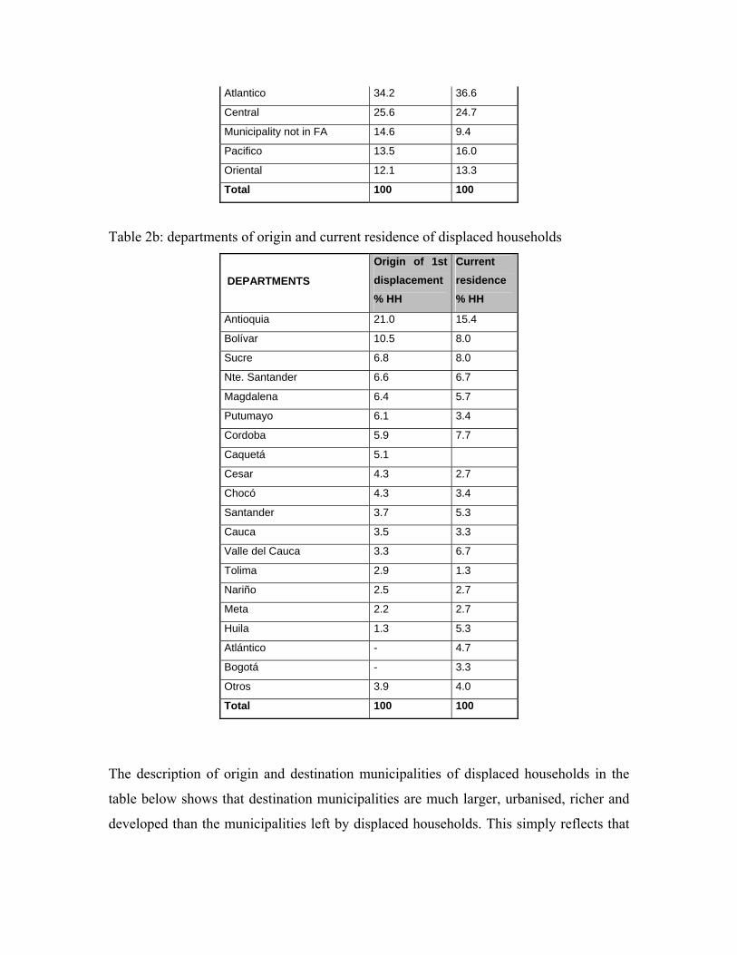
Atlantico 34.2 36.6

Central 25.6 24.7

Municipality not in FA 14.6 9.4

Pacifico 13.5 16.0

Oriental 12.1 13.3

Total 100 100

Table 2b: departments of origin and current residence of displaced households

DEPARTMENTS

Origin of 1st displacement % HH

Current residence % HH

Antioquia 21.0 15.4

Bolívar 10.5 8.0

Sucre 6.8 8.0

Nte. Santander 6.6 6.7

Magdalena 6.4 5.7

Putumayo 6.1 3.4

Cordoba 5.9 7.7

Caquetá 5.1

Cesar 4.3 2.7

Chocó 4.3 3.4

Santander 3.7 5.3

Cauca 3.5 3.3

Valle del Cauca 3.3 6.7

Tolima 2.9 1.3

Nariño 2.5 2.7

Meta 2.2 2.7

Huila 1.3 5.3

Atlántico - 4.7

Bogotá - 3.3

Otros 3.9 4.0

Total 100 100

The description of origin and destination municipalities of displaced households in the

table below shows that destination municipalities are much larger, urbanised, richer and

developed than the municipalities left by displaced households. This simply reflects that

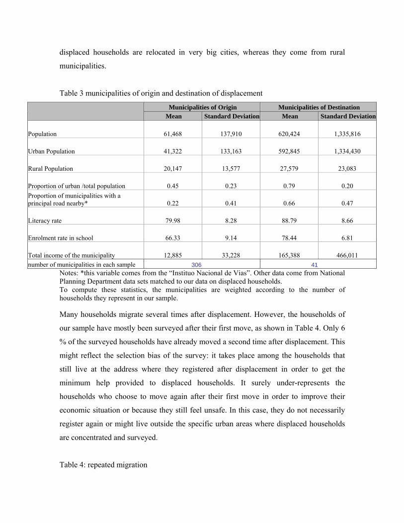
displaced households are relocated in very big cities, whereas they come from rural

municipalities.

Table 3 municipalities of origin and destination of displacement

Municipalities of Origin Municipalities of Destination Mean Standard Deviation Mean Standard Deviation

Population 61,468 137,910 620,424 1,335,816

Urban Population 41,322 133,163 592,845 1,334,430

Rural Population 20,147 13,577 27,579 23,083

Proportion of urban /total population 0.45 0.23 0.79 0.20 Proportion of municipalities with a principal road nearby* 0.22 0.41 0.66 0.47

Literacy rate 79.98 8.28 88.79 8.66

Enrolment rate in school 66.33 9.14 78.44 6.81

Total income of the municipality 12,885 33,228 165,388 466,011 number of municipalities in each sample 306 41

Notes: *this variable comes from the “Instituo Nacional de Vias”. Other data come from National Planning Department data sets matched to our data on displaced households. To compute these statistics, the municipalities are weighted according to the number of households they represent in our sample. Many households migrate several times after displacement. However, the households of

our sample have mostly been surveyed after their first move, as shown in Table 4. Only 6

% of the surveyed households have already moved a second time after displacement. This

might reflect the selection bias of the survey: it takes place among the households that

still live at the address where they registered after displacement in order to get the

minimum help provided to displaced households. It surely under-represents the

households who choose to move again after their first move in order to improve their

economic situation or because they still feel unsafe. In this case, they do not necessarily

register again or might live outside the specific urban areas where displaced households

are concentrated and surveyed.

Table 4: repeated migration

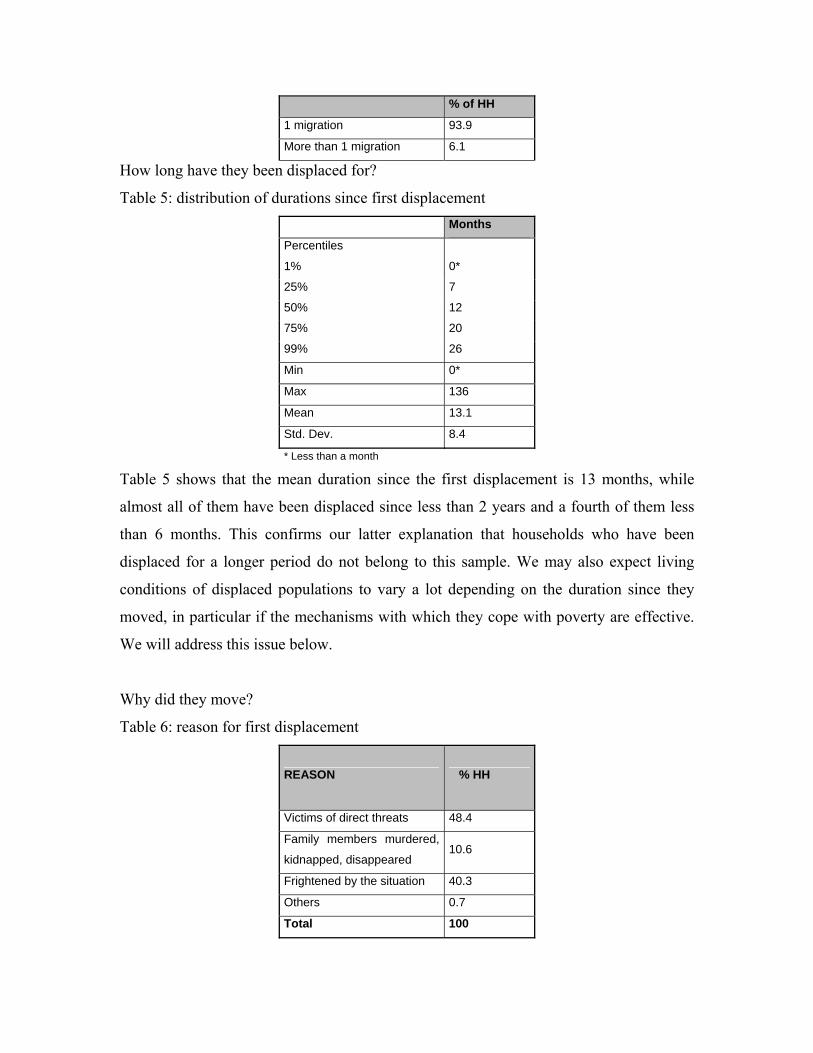
% of HH

1 migration 93.9

More than 1 migration 6.1

How long have they been displaced for?

Table 5: distribution of durations since first displacement Months

Percentiles

1% 0*

25% 7

50% 12

75% 20

99% 26

Min 0*

Max 136

Mean 13.1

Std. Dev. 8.4

* Less than a month

Table 5 shows that the mean duration since the first displacement is 13 months, while

almost all of them have been displaced since less than 2 years and a fourth of them less

than 6 months. This confirms our latter explanation that households who have been

displaced for a longer period do not belong to this sample. We may also expect living

conditions of displaced populations to vary a lot depending on the duration since they

moved, in particular if the mechanisms with which they cope with poverty are effective.

We will address this issue below.

Why did they move?

Table 6: reason for first displacement

REASON % HH

Victims of direct threats 48.4

Family members murdered,

kidnapped, disappeared 10.6

Frightened by the situation 40.3

Others 0.7

Total 100

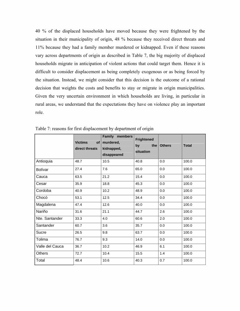
40 % of the displaced households have moved because they were frightened by the

situation in their municipality of origin, 48 % because they received direct threats and

11% because they had a family member murdered or kidnapped. Even if these reasons

vary across departments of origin as described in Table 7, the big majority of displaced

households migrate in anticipation of violent actions that could target them. Hence it is

difficult to consider displacement as being completely exogenous or as being forced by

the situation. Instead, we might consider that this decision is the outcome of a rational

decision that weights the costs and benefits to stay or migrate in origin municipalities.

Given the very uncertain environment in which households are living, in particular in

rural areas, we understand that the expectations they have on violence play an important

role.

Table 7: reasons for first displacement by department of origin

Victims of direct threats

Family members murdered, kidnapped, disappeared

Frightened by the situation

Others Total

Antioquia 48.7 10.5 40.8 0.0 100.0

Bolívar 27.4 7.6 65.0 0.0 100.0

Cauca 63.5 21.2 15.4 0.0 100.0

Cesar 35.9 18.8 45.3 0.0 100.0

Cordoba 40.9 10.2 48.9 0.0 100.0

Chocó 53.1 12.5 34.4 0.0 100.0

Magdalena 47.4 12.6 40.0 0.0 100.0

Nariño 31.6 21.1 44.7 2.6 100.0

Nte. Santander 33.3 4.0 60.6 2.0 100.0

Santander 60.7 3.6 35.7 0.0 100.0

Sucre 26.5 9.8 63.7 0.0 100.0

Tolima 76.7 9.3 14.0 0.0 100.0

Valle del Cauca 36.7 10.2 46.9 6.1 100.0

Others 72.7 10.4 15.5 1.4 100.0

Total 48.4 10.6 40.3 0.7 100.0

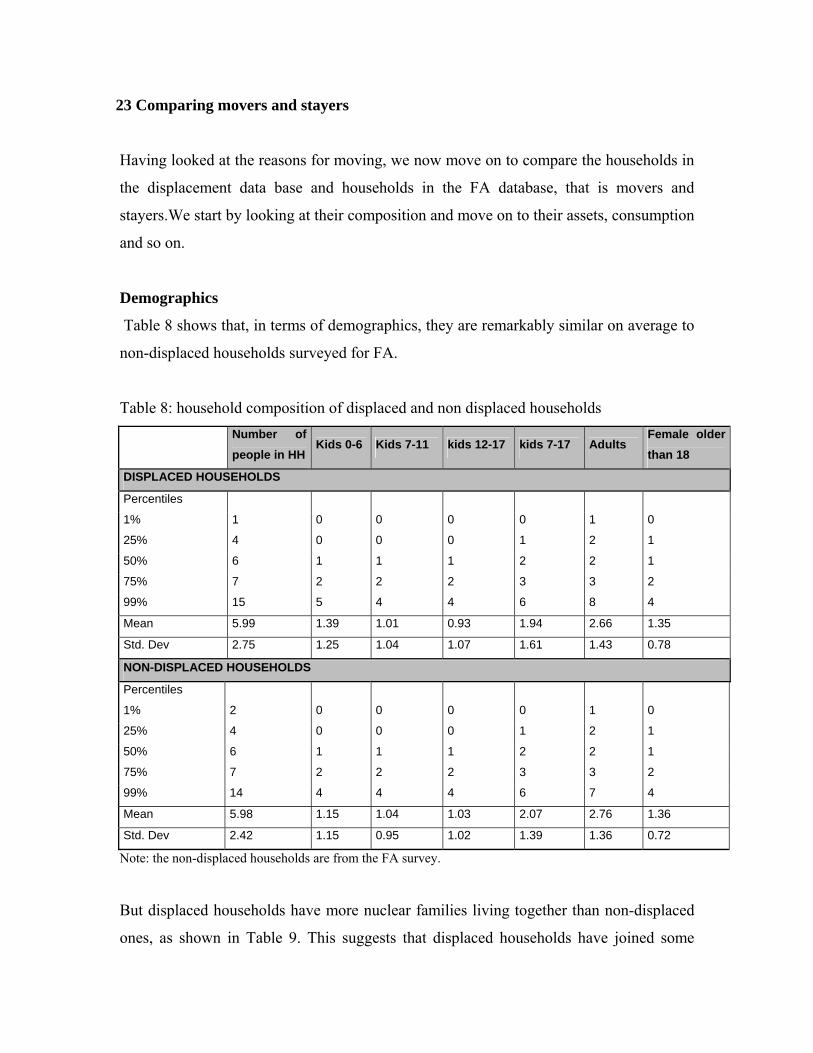
23 Comparing movers and stayers

Having looked at the reasons for moving, we now move on to compare the households in

the displacement data base and households in the FA database, that is movers and

stayers.We start by looking at their composition and move on to their assets, consumption

and so on.

Demographics

Table 8 shows that, in terms of demographics, they are remarkably similar on average to

non-displaced households surveyed for FA.

Table 8: household composition of displaced and non displaced households

Number of people in HH

Kids 0-6 Kids 7-11 kids 12-17 kids 7-17 Adults Female older than 18

DISPLACED HOUSEHOLDS

Percentiles

1% 1 0 0 0 0 1 0

25% 4 0 0 0 1 2 1

50% 6 1 1 1 2 2 1

75% 7 2 2 2 3 3 2

99% 15 5 4 4 6 8 4

Mean 5.99 1.39 1.01 0.93 1.94 2.66 1.35

Std. Dev 2.75 1.25 1.04 1.07 1.61 1.43 0.78

NON-DISPLACED HOUSEHOLDS

Percentiles

1% 2 0 0 0 0 1 0

25% 4 0 0 0 1 2 1

50% 6 1 1 1 2 2 1

75% 7 2 2 2 3 3 2

99% 14 4 4 4 6 7 4

Mean 5.98 1.15 1.04 1.03 2.07 2.76 1.36

Std. Dev 2.42 1.15 0.95 1.02 1.39 1.36 0.72

Note: the non-displaced households are from the FA survey.

But displaced households have more nuclear families living together than non-displaced

ones, as shown in Table 9. This suggests that displaced households have joined some

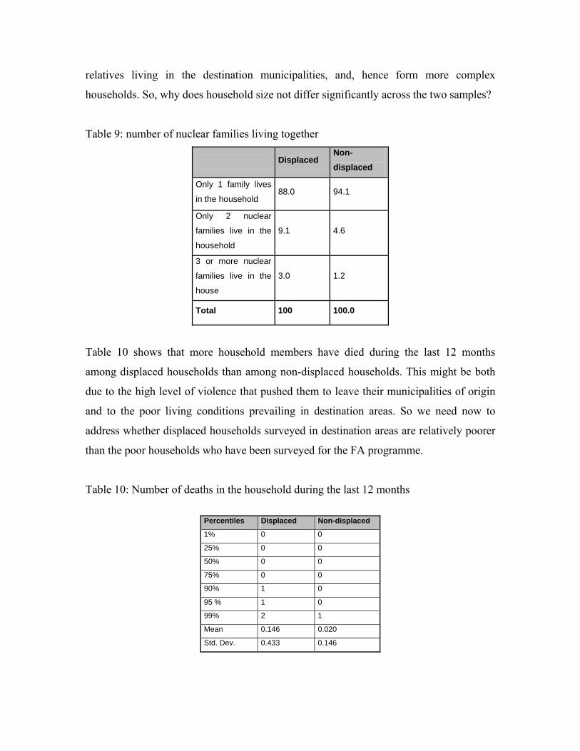
relatives living in the destination municipalities, and, hence form more complex

households. So, why does household size not differ significantly across the two samples?

Table 9: number of nuclear families living together

Displaced Non-displaced

Only 1 family lives

in the household 88.0 94.1

Only 2 nuclear

families live in the

household

9.1 4.6

3 or more nuclear

families live in the

house

3.0 1.2

Total 100 100.0

Table 10 shows that more household members have died during the last 12 months

among displaced households than among non-displaced households. This might be both

due to the high level of violence that pushed them to leave their municipalities of origin

and to the poor living conditions prevailing in destination areas. So we need now to

address whether displaced households surveyed in destination areas are relatively poorer

than the poor households who have been surveyed for the FA programme.

Table 10: Number of deaths in the household during the last 12 months

Percentiles Displaced Non-displaced

1% 0 0

25% 0 0

50% 0 0

75% 0 0

90% 1 0

95 % 1 0

99% 2 1

Mean 0.146 0.020

Std. Dev. 0.433 0.146

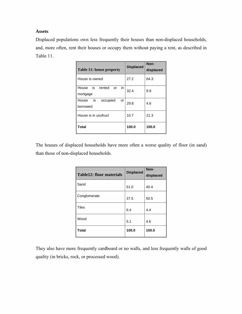
Assets

Displaced populations own less frequently their houses than non-displaced households,

and, more often, rent their houses or occupy them without paying a rent, as described in

Table 11.

Table 11: house property Displaced

Non-displaced

House is owned 27.2 64.3

House is rented or in

mortgage 32.4 9.9

House is occupied or

borrowed 29.8 4.6

House is in usufruct 10.7 21.3

Total 100.0 100.0

The houses of displaced households have more often a worse quality of floor (in sand)

than those of non-displaced households.

Table12: floor materials DisplacedNon-displaced

Sand 51.0 40.4

Conglomerate 37.5 50.5

Tiles 6.4 4.4

Wood 5.1 4.6

Total 100.0 100.0

They also have more frequently cardboard or no walls, and less frequently walls of good

quality (in bricks, rock, or processed wood).

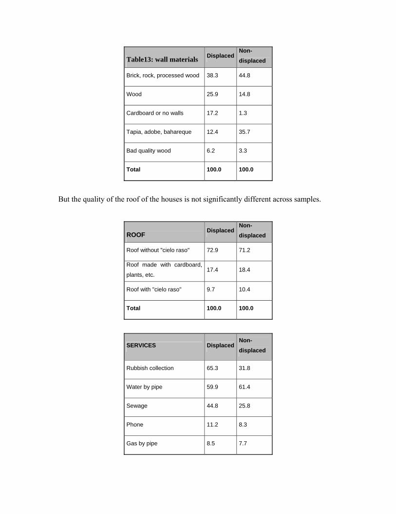
Table13: wall materials DisplacedNon-displaced

Brick, rock, processed wood 38.3 44.8

Wood 25.9 14.8

Cardboard or no walls 17.2 1.3

Tapia, adobe, bahareque 12.4 35.7

Bad quality wood 6.2 3.3

Total 100.0 100.0

But the quality of the roof of the houses is not significantly different across samples.

ROOF Displaced

Non-displaced

Roof without "cielo raso" 72.9 71.2

Roof made with cardboard,

plants, etc. 17.4 18.4

Roof with "cielo raso" 9.7 10.4

Total 100.0 100.0

SERVICES DisplacedNon-displaced

Rubbish collection 65.3 31.8

Water by pipe 59.9 61.4

Sewage 44.8 25.8

Phone 11.2 8.3

Gas by pipe 8.5 7.7

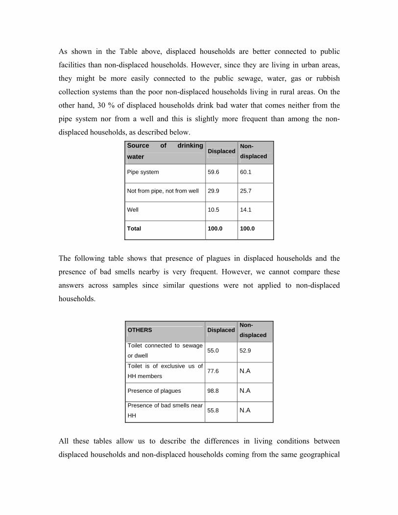
As shown in the Table above, displaced households are better connected to public

facilities than non-displaced households. However, since they are living in urban areas,

they might be more easily connected to the public sewage, water, gas or rubbish

collection systems than the poor non-displaced households living in rural areas. On the

other hand, 30 % of displaced households drink bad water that comes neither from the

pipe system nor from a well and this is slightly more frequent than among the non-

displaced households, as described below.

Source of drinking water

DisplacedNon-displaced

Pipe system 59.6 60.1

Not from pipe, not from well 29.9 25.7

Well 10.5 14.1

Total 100.0 100.0

The following table shows that presence of plagues in displaced households and the

presence of bad smells nearby is very frequent. However, we cannot compare these

answers across samples since similar questions were not applied to non-displaced

households.

OTHERS DisplacedNon-displaced

Toilet connected to sewage

or dwell 55.0 52.9

Toilet is of exclusive us of

HH members 77.6 N.A

Presence of plagues 98.8 N.A

Presence of bad smells near

HH 55.8 N.A

All these tables allow us to describe the differences in living conditions between

displaced households and non-displaced households coming from the same geographical

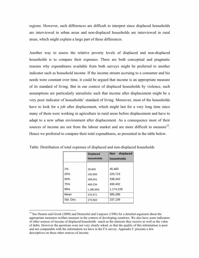
regions. However, such differences are difficult to interpret since displaced households

are interviewed in urban areas and non-displaced households are interviewed in rural

areas, which might explain a large part of these differences.

Another way to assess the relative poverty levels of displaced and non-displaced

households is to compare their expenses. There are both conceptual and pragmatic

reasons why expenditures available from both surveys might be preferred to another

indicator such as household income. If the income stream accruing to a consumer and his

needs were constant over time, it could be argued that income is an appropriate measure

of its standard of living. But in our context of displaced households by violence, such

assumptions are particularly unrealistic such that income after displacement might be a

very poor indicator of households’ standard of living. Moreover, most of the households

have to look for a job after displacement, which might last for a very long time since

many of them were working in agriculture in rural areas before displacement and have to

adapt to a new urban environment after displacement. As a consequence most of their

sources of income are not from the labour market and are more difficult to measure19.

Hence we preferred to compare their total expenditures, as presented in the table below.

Table: Distribution of total expenses of displaced and non-displaced households

Displaced households

Non displaced households

1% 29,600 45,483

25% 192,600 225,723

50% 308,501 338,342

75% 469,234 490,402

99% 1,380,803 1,174,228

Mean 370,571 385,286

Std. Dev. 273,563 237,109

19 See Deaton and Grosh (2000) and Hentschel and Lanjouw (1996) for a detailed argument about the appropriate measures welfare measure in the context of developing countries. We also have some indicators of other sources of income of displaced households suach as the interests they receive as well as the value of debts. However the questions were not very clearly asked, so that the quality of this information is poor and not comparable with the information we have in the FA survey. Appendix C presents a few descriptives on these other sources of income.

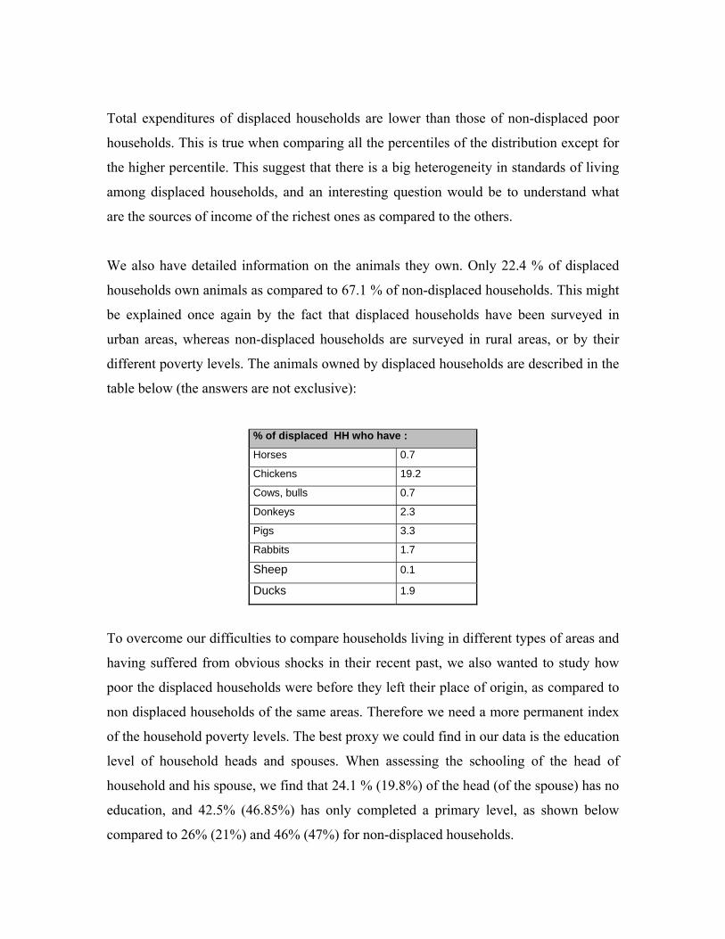
Total expenditures of displaced households are lower than those of non-displaced poor

households. This is true when comparing all the percentiles of the distribution except for

the higher percentile. This suggest that there is a big heterogeneity in standards of living

among displaced households, and an interesting question would be to understand what

are the sources of income of the richest ones as compared to the others.

We also have detailed information on the animals they own. Only 22.4 % of displaced

households own animals as compared to 67.1 % of non-displaced households. This might

be explained once again by the fact that displaced households have been surveyed in

urban areas, whereas non-displaced households are surveyed in rural areas, or by their

different poverty levels. The animals owned by displaced households are described in the

table below (the answers are not exclusive):

% of displaced HH who have :

Horses 0.7

Chickens 19.2

Cows, bulls 0.7

Donkeys 2.3

Pigs 3.3

Rabbits 1.7

Sheep 0.1

Ducks 1.9

To overcome our difficulties to compare households living in different types of areas and

having suffered from obvious shocks in their recent past, we also wanted to study how

poor the displaced households were before they left their place of origin, as compared to

non displaced households of the same areas. Therefore we need a more permanent index

of the household poverty levels. The best proxy we could find in our data is the education

level of household heads and spouses. When assessing the schooling of the head of

household and his spouse, we find that 24.1 % (19.8%) of the head (of the spouse) has no

education, and 42.5% (46.85%) has only completed a primary level, as shown below

compared to 26% (21%) and 46% (47%) for non-displaced households.

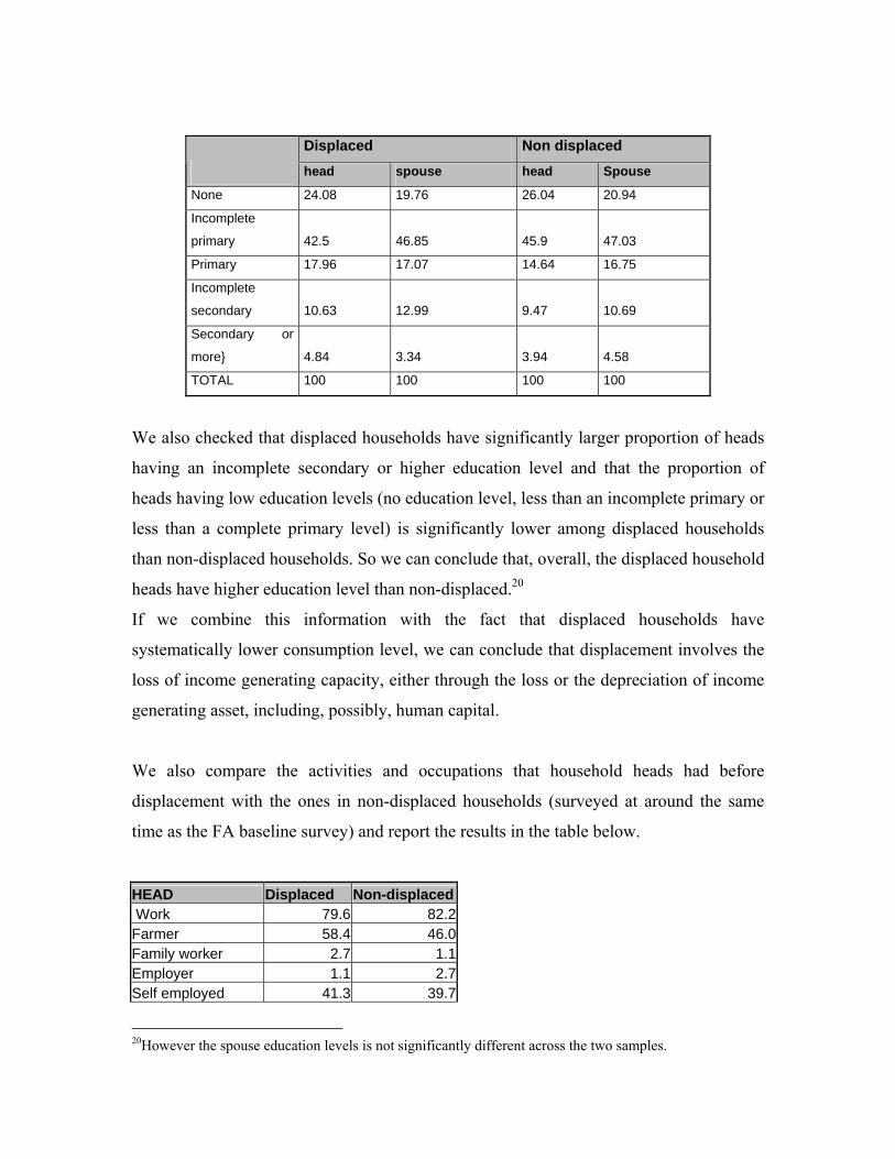
Displaced Non displaced head spouse head Spouse

None 24.08 19.76 26.04 20.94

Incomplete

primary 42.5 46.85 45.9 47.03

Primary 17.96 17.07 14.64 16.75

Incomplete

secondary 10.63 12.99 9.47 10.69

Secondary or

more} 4.84 3.34 3.94 4.58

TOTAL 100 100 100 100

We also checked that displaced households have significantly larger proportion of heads

having an incomplete secondary or higher education level and that the proportion of

heads having low education levels (no education level, less than an incomplete primary or

less than a complete primary level) is significantly lower among displaced households

than non-displaced households. So we can conclude that, overall, the displaced household

heads have higher education level than non-displaced.20

If we combine this information with the fact that displaced households have

systematically lower consumption level, we can conclude that displacement involves the

loss of income generating capacity, either through the loss or the depreciation of income

generating asset, including, possibly, human capital.

We also compare the activities and occupations that household heads had before

displacement with the ones in non-displaced households (surveyed at around the same

time as the FA baseline survey) and report the results in the table below.

HEAD Displaced Non-displaced Work 79.6 82.2Farmer 58.4 46.0Family worker 2.7 1.1Employer 1.1 2.7Self employed 41.3 39.7

20However the spouse education levels is not significantly different across the two samples.

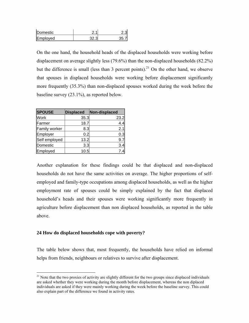
Domestic 2.1 2.3Employed 32.3 35.7

On the one hand, the household heads of the displaced households were working before

displacement on average slightly less (79.6%) than the non-displaced households (82.2%)

but the difference is small (less than 3 percent points).21 On the other hand, we observe

that spouses in displaced households were working before displacement significantly

more frequently (35.3%) than non-displaced spouses worked during the week before the

baseline survey (23.1%), as reported below.

SPOUSE Displaced Non-displaced Work 35.3 23.2Farmer 18.7 4.4Family worker 8.3 2.1Employer 0.2 0.3Self employed 13.2 9.7Domestic 3.3 3.4Employed 10.5 7.4

Another explanation for these findings could be that displaced and non-displaced

households do not have the same activities on average. The higher proportions of self-

employed and family-type occupations among displaced households, as well as the higher

employment rate of spouses could be simply explained by the fact that displaced

household’s heads and their spouses were working significantly more frequently in

agriculture before displacement than non displaced households, as reported in the table

above.

24 How do displaced households cope with poverty?

The table below shows that, most frequently, the households have relied on informal

helps from friends, neighbours or relatives to survive after displacement.

21 Note that the two proxies of activity are slightly different for the two groups since displaced individuals are asked whether they were working during the month before displacement, whereas the non diplaced individuals are asked if they were mainly working during the week before the baseline survey. This could also explain part of the difference we found in activity rates.

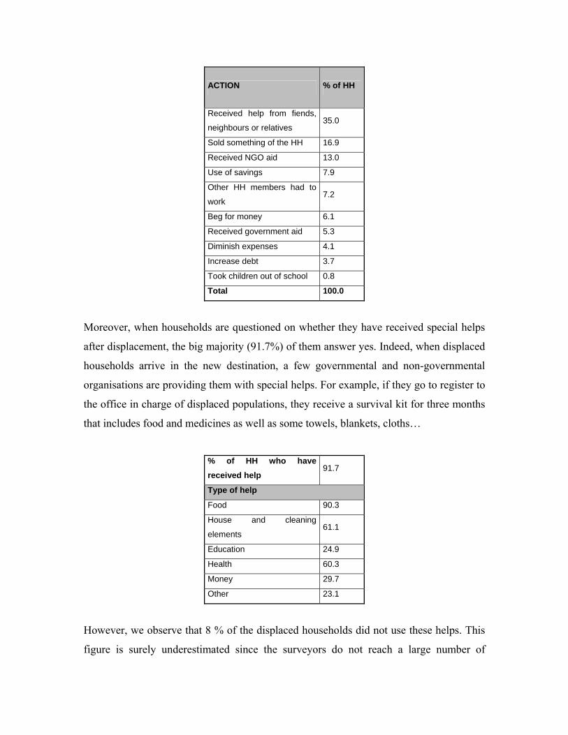
ACTION % of HH

Received help from fiends,

neighbours or relatives 35.0

Sold something of the HH 16.9

Received NGO aid 13.0

Use of savings 7.9

Other HH members had to

work 7.2

Beg for money 6.1

Received government aid 5.3

Diminish expenses 4.1

Increase debt 3.7

Took children out of school 0.8

Total 100.0

Moreover, when households are questioned on whether they have received special helps

after displacement, the big majority (91.7%) of them answer yes. Indeed, when displaced

households arrive in the new destination, a few governmental and non-governmental

organisations are providing them with special helps. For example, if they go to register to

the office in charge of displaced populations, they receive a survival kit for three months

that includes food and medicines as well as some towels, blankets, cloths…

% of HH who have received help

91.7

Type of help

Food 90.3

House and cleaning

elements 61.1

Education 24.9

Health 60.3

Money 29.7

Other 23.1

However, we observe that 8 % of the displaced households did not use these helps. This

figure is surely underestimated since the surveyors do not reach a large number of

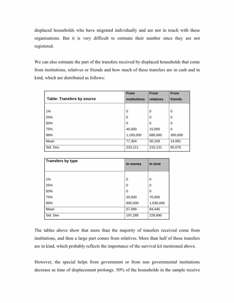
displaced households who have migrated individually and are not in touch with these

organisations. But it is very difficult to estimate their number since they are not

registered.

We can also estimate the part of the transfers received by displaced households that come

from institutions, relatives or friends and how much of these transfers are in cash and in

kind, which are distributed as follows:

Table: Transfers by source From institutions

From relatives

From friends

1% 0 0 0

25% 0 0 0

50% 0 0 0

75% 45,000 15,000 0

99% 1,100,000 680,000 300,000

Mean 77,304 50,159 14,081

Std. Dev. 233,211 215,131 65,076

Transfers by type

In money In kind

1% 0 0

25% 0 0

50% 0 0

75% 20,000 70,000

99% 900,000 1,030,000

Mean 57,099 84,445

Std. Dev. 197,285 229,890

The tables above show that more than the majority of transfers received come from

institutions, and then a large part comes from relatives. More than half of these transfers

are in kind, which probably reflects the importance of the survival kit mentioned above.

However, the special helps from government or from non governmental institutions

decrease as time of displacement prolongs. 50% of the households in the sample receive

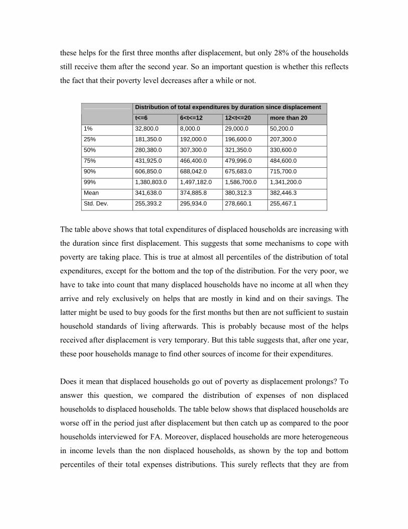
these helps for the first three months after displacement, but only 28% of the households

still receive them after the second year. So an important question is whether this reflects

the fact that their poverty level decreases after a while or not.

Distribution of total expenditures by duration since displacement

t<=6 6<t<=12 12<t<=20 more than 20

1% 32,800.0 8,000.0 29,000.0 50,200.0

25% 181,350.0 192,000.0 196,600.0 207,300.0

50% 280,380.0 307,300.0 321,350.0 330,600.0

75% 431,925.0 466,400.0 479,996.0 484,600.0

90% 606,850.0 688,042.0 675,683.0 715,700.0

99% 1,380,803.0 1,497,182.0 1,586,700.0 1,341,200.0

Mean 341,638.0 374,885.8 380,312.3 382,446.3

Std. Dev. 255,393.2 295,934.0 278,660.1 255,467.1

The table above shows that total expenditures of displaced households are increasing with

the duration since first displacement. This suggests that some mechanisms to cope with

poverty are taking place. This is true at almost all percentiles of the distribution of total

expenditures, except for the bottom and the top of the distribution. For the very poor, we

have to take into count that many displaced households have no income at all when they

arrive and rely exclusively on helps that are mostly in kind and on their savings. The

latter might be used to buy goods for the first months but then are not sufficient to sustain

household standards of living afterwards. This is probably because most of the helps

received after displacement is very temporary. But this table suggests that, after one year,

these poor households manage to find other sources of income for their expenditures.

Does it mean that displaced households go out of poverty as displacement prolongs? To

answer this question, we compared the distribution of expenses of non displaced

households to displaced households. The table below shows that displaced households are

worse off in the period just after displacement but then catch up as compared to the poor

households interviewed for FA. Moreover, displaced households are more heterogeneous

in income levels than the non displaced households, as shown by the top and bottom

percentiles of their total expenses distributions. This surely reflects that they are from

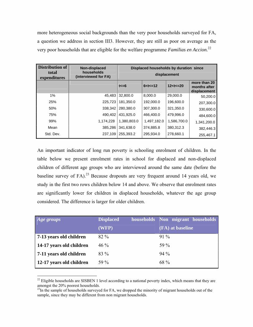
more heterogeneous social backgrounds than the very poor households surveyed for FA,

a question we address in section III3. However, they are still as poor on average as the

very poor households that are eligible for the welfare programme Familias en Accion.22

Distribution of total

expenditures

Non-displaced households

(interviewed for FA)

Displaced households by duration since displacement

t<=6 6<t<=12 12<t<=20

more than 20 months after displacement

1% 45,483 32,800.0 8,000.0 29,000.0 50,200.025% 225,723 181,350.0 192,000.0 196,600.0 207,300.050% 338,342 280,380.0 307,300.0 321,350.0 330,600.075% 490,402 431,925.0 466,400.0 479,996.0 484,600.099% 1,174,228 1,380,803.0 1,497,182.0 1,586,700.0 1,341,200.0Mean 385,286 341,638.0 374,885.8 380,312.3 382,446.3

Std. Dev. 237,109 255,393.2 295,934.0 278,660.1 255,467.1

An important indicator of long run poverty is schooling enrolment of children. In the

table below we present enrolment rates in school for displaced and non-displaced

children of different age groups who are interviewed around the same date (before the

baseline survey of FA).23 Because dropouts are very frequent around 14 years old, we

study in the first two rows children below 14 and above. We observe that enrolment rates

are significantly lower for children in displaced households, whatever the age group

considered. The difference is larger for older children.

Age groups Displaced households

(WFP)

Non migrant households

(FA) at baseline

7-13 years old children 82 % 91 %

14-17 years old children 46 % 59 %

7-11 years old children 83 % 94 %

12-17 years old children 59 % 68 %

22 Eligible households are SISBEN 1 level according to a national poverty index, which means that they are amongst the 20% poorest households. 23In the sample of households surveyed for FA, we dropped the minority of migrant households out of the sample, since they may be different from non migrant households.

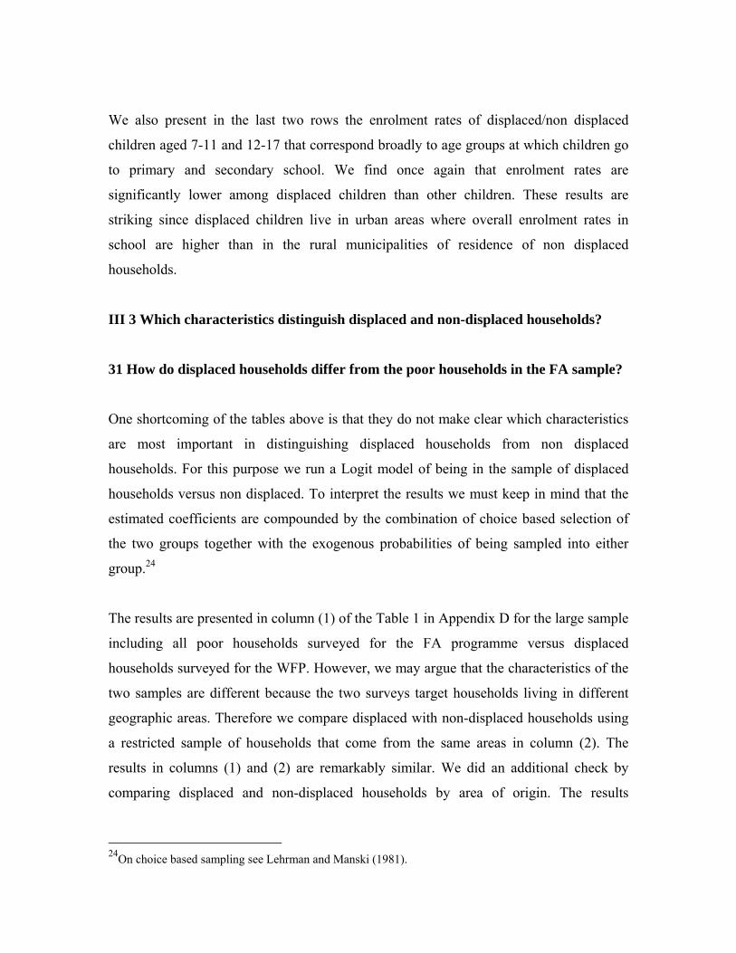
We also present in the last two rows the enrolment rates of displaced/non displaced

children aged 7-11 and 12-17 that correspond broadly to age groups at which children go

to primary and secondary school. We find once again that enrolment rates are

significantly lower among displaced children than other children. These results are

striking since displaced children live in urban areas where overall enrolment rates in

school are higher than in the rural municipalities of residence of non displaced

households.

III 3 Which characteristics distinguish displaced and non-displaced households?

31 How do displaced households differ from the poor households in the FA sample?

One shortcoming of the tables above is that they do not make clear which characteristics

are most important in distinguishing displaced households from non displaced

households. For this purpose we run a Logit model of being in the sample of displaced

households versus non displaced. To interpret the results we must keep in mind that the

estimated coefficients are compounded by the combination of choice based selection of

the two groups together with the exogenous probabilities of being sampled into either

group.24

The results are presented in column (1) of the Table 1 in Appendix D for the large sample

including all poor households surveyed for the FA programme versus displaced

households surveyed for the WFP. However, we may argue that the characteristics of the

two samples are different because the two surveys target households living in different

geographic areas. Therefore we compare displaced with non-displaced households using

a restricted sample of households that come from the same areas in column (2). The

results in columns (1) and (2) are remarkably similar. We did an additional check by

comparing displaced and non-displaced households by area of origin. The results

24On choice based sampling see Lehrman and Manski (1981).

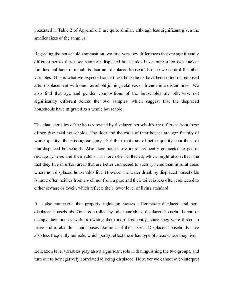
presented in Table 2 of Appendix D are quite similar, although less significant given the

smaller sizes of the samples.

Regarding the household composition, we find very few differences that are significantly

different across these two samples: displaced households have more often two nuclear

families and have more adults than non displaced households once we control for other

variables. This is what we expected since these households have been often recomposed

after displacement with one household joining relatives or friends in a distant area. We

also find that age and gender compositions of the households are otherwise not

significantly different across the two samples, which suggest that the displaced

households have migrated as a whole household.

The characteristics of the houses owned by displaced households are different from those

of non displaced households. The floor and the walls of their houses are significantly of

worse quality -the missing category-, but their roofs are of better quality than those of

non-displaced households. Also their houses are more frequently connected to gas or

sewage systems and their rubbish is more often collected, which might also reflect the

fact they live in urban areas that are better connected to such systems than in rural areas

where non displaced households live. However the water drunk by displaced households

is more often neither from a well nor from a pipe and their toilet is less often connected to

either sewage or dwell, which reflects their lower level of living standard.

It is also noticeable that property rights on houses differentiate displaced and non-

displaced households. Once controlled by other variables, displaced households rent or

occupy their houses without owning them more frequently, since they were forced to

leave and to abandon their houses like most of their assets. Displaced households have

also less frequently animals, which partly reflect the urban type of areas where they live.

Education level variables play also a significant role in distinguishing the two groups, and

turn out to be negatively correlated to being displaced. However we cannot over-interpret

these correlations in a causal way since many of the other control characteristics used in

our regression framework measured after displacement are endogenous.

To have a better idea of which characteristics differentiate ex ante non-displaced and

displaced households, we kept in a separate regression the variables that are

predetermined to displacement such as activities and occupations before moving,

education levels of household heads and spouses, or likely to be more permanent

characteristics of the household like the structure per age of children. The results

presented in Table 3 of Appendix D show that displaced households have significantly

more educated heads and spouses, and work more often in agriculture than non-displaced

households. However, the fact that these variables are predetermined to mobility

decisions does not, of course, guarantee exogeneity. As a check for robustness, we drop

the controls for activities and occupations before moving that are likely to be endogenous

to mobility decisions. The table below shows that the result that displaced households are

headed by individuals with higher education achievement is a robust one:

logit displaced/non displaced (1) (2)

whole sample Common

sample

Primary level not completed by head -0.01 -0.03

(0.09) (0.09)

Primary level completed by head 0.25 0.33

(0.11)* (0.12)**

Secondary level not completed by head

and more

0.09 0.10

(0.12) (0.13)

Primary level not completed by spouse 0.02 0.03

(0.09) (0.10)

Primary level completed by spouse -0.03 0.15

(0.11) (0.12)

Secondary level not completed by -0.02 0.05

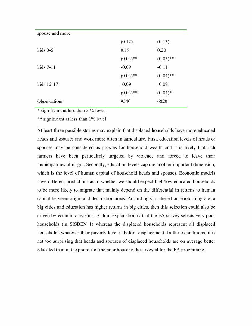
spouse and more

(0.12) (0.13)

kids 0-6 0.19 0.20

(0.03)** (0.03)**

kids 7-11 -0.09 -0.11

(0.03)** (0.04)**

kids 12-17 -0.09 -0.09

(0.03)** (0.04)*

Observations 9540 6820

* significant at less than 5 % level

** significant at less than 1% level At least three possible stories may explain that displaced households have more educated

heads and spouses and work more often in agriculture. First, education levels of heads or

spouses may be considered as proxies for household wealth and it is likely that rich

farmers have been particularly targeted by violence and forced to leave their

municipalities of origin. Secondly, education levels capture another important dimension,

which is the level of human capital of household heads and spouses. Economic models

have different predictions as to whether we should expect high/low educated households

to be more likely to migrate that mainly depend on the differential in returns to human

capital between origin and destination areas. Accordingly, if these households migrate to

big cities and education has higher returns in big cities, then this selection could also be

driven by economic reasons. A third explanation is that the FA survey selects very poor

households (in SISBEN 1) whereas the displaced households represent all displaced

households whatever their poverty level is before displacement. In these conditions, it is

not too surprising that heads and spouses of displaced households are on average better

educated than in the poorest of the poor households surveyed for the FA programme.

32 How do displaced households differ from the households interviewed for FA and migrated out of their municipalities of origin? Very similarly, we studied also the characteristics that differentiate migrant households

from displaced households. This is important to understand if the very poor households

who chose to migrate are comparable to displaced households.

Column (1) in Table 4 of Appendix D shows that a couple of variables are significant in

explaining differences across these samples. These are the characteristics of the house in

which the households are living, like the quality of walls that are worse in displaced

households or the type of roof (better), as well as their property rights: displaced

households rent or occupy their houses more frequently, and have houses in usufruct less

frequently than migrant households. However, we have to bear in mind once again that

these characteristics are observed before migration for the FA sample, whereas they

describe houses after displacement for the other sample. We also find that displaced

households have fewer animals than migrant households have before migration. Once

again, we cannot infer much from these results since this partly reflects that living

conditions after displacement into urban areas are very different from rural areas where

the FA survey was implemented.

To overcome these problems we compare the characteristics of displaced and migrant

households that are predetermined to migration. The results presented in columns (2) of

Table 4 show that education levels of the heads become significantly positive in

distinguishing displaced households from migrants, together with a few variables

characterising the occupation of household heads and spouses and household

composition. According to these results, displaced household heads are significantly

more educated than migrants and displaced household heads and spouses were more

frequently self-employed and farmers in their origin municipality. Once again, however,

we cannot exclude that these results may also reflect the selection bias of the two

samples.

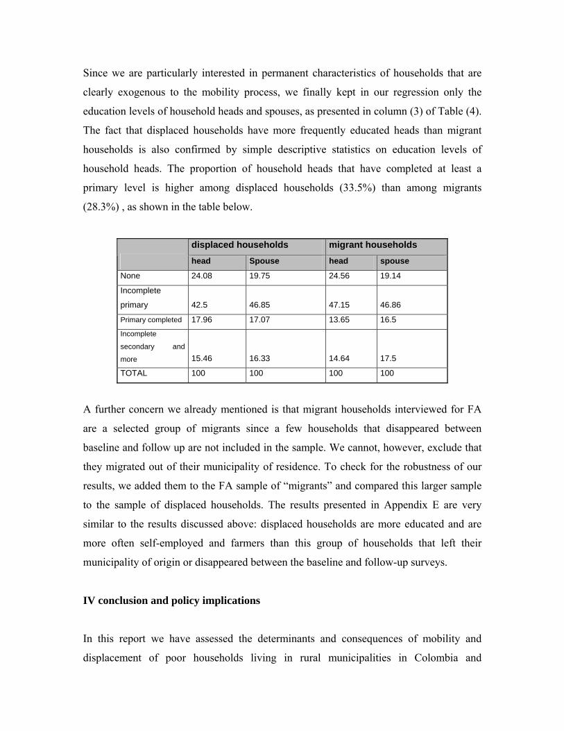
Since we are particularly interested in permanent characteristics of households that are

clearly exogenous to the mobility process, we finally kept in our regression only the

education levels of household heads and spouses, as presented in column (3) of Table (4).

The fact that displaced households have more frequently educated heads than migrant

households is also confirmed by simple descriptive statistics on education levels of

household heads. The proportion of household heads that have completed at least a

primary level is higher among displaced households (33.5%) than among migrants

(28.3%) , as shown in the table below.

displaced households migrant households head Spouse head spouse

None 24.08 19.75 24.56 19.14

Incomplete

primary 42.5 46.85 47.15 46.86

Primary completed 17.96 17.07 13.65 16.5

Incomplete

secondary and

more 15.46 16.33 14.64 17.5

TOTAL 100 100 100 100

A further concern we already mentioned is that migrant households interviewed for FA

are a selected group of migrants since a few households that disappeared between

baseline and follow up are not included in the sample. We cannot, however, exclude that

they migrated out of their municipality of residence. To check for the robustness of our

results, we added them to the FA sample of “migrants” and compared this larger sample

to the sample of displaced households. The results presented in Appendix E are very

similar to the results discussed above: displaced households are more educated and are

more often self-employed and farmers than this group of households that left their

municipality of origin or disappeared between the baseline and follow-up surveys.

IV conclusion and policy implications

In this report we have assessed the determinants and consequences of mobility and

displacement of poor households living in rural municipalities in Colombia and

characterised the profile of these poor households versus those living in displaced

communities in urban areas where specific surveys have been implemented.

We have shown that household decisions to leave rural municipalities of residence

respond strongly and positively to the level of violence in municipalities. We found that

receiving the programme decreases migration if the level of violence is not unduly high.

We have also measured that the negative effect of violence on migration more than

offsets the positive effect played by violence incidence for the big majority of villages of

our sample. This suggests interesting policy implications if a government’s aim were to

slow down the migration flows out of the municipalities that are destabilised by high

levels of violence. Our results show, however, that welfare programmes such as FA are

not effective at curbing migration in municipalities with very high level of violence. This

confirms that migration decisions and displacement are of different nature, and warns us

to be careful when extrapolating our results to advocate policy interventions in

emergency situations that push populations to migrate massively. We also find that

migration decisions are strongly determined by household property rights, type of

insurance held by households, type of jobs of household heads and spouses and wage

levels in municipalities of origin. This also suggests that policy measures oriented

towards rural development, access to housing market and health insurance would be

effective at encouraging economic migration between rural municipalities of Colombia.

We have also described the consequences of migration on the 113 households that are

tracked by the surveyors at follow-up, as well as the consequences of displacement using

a special survey made in relocation areas of displaced households. We found a contrasted

picture for migrant households. On one hand, households are looking for better jobs in

urban areas and are pulled by the presence of friends or relative in destination areas. On

the other hand, migration entails severe costs for these very poor households. Many of

them sold goods below their market value or lost goods and land that they could not carry

with them. Most impressive is the fact that even though displaced households have higher

human capital, they have a considerably lower level of consumption, probably reflecting

a loss in productive assets, including specific human capital. And these losses can have

important intergenerational consequences: we observed that enrolment rates among the

children of displaced and migrant households are considerably lower than among other

households.

One has to be cautious, however, while assessing overall costs and benefits of migration

based on data gathered within the year following migration. If one wants to study the

impact of migration on well being of these households, we would need more follow-up

surveys or longer term outcomes since conditions at the time they arrive are likely to

change very fast, depending on the labour market and economic prospects in destination

areas. However, given the costs entailed by displacement and migration, it is maybe not

too surprising if very few households have migrated out of the rural municipalities

interviewed for the evaluation of Familias en Accion as observed between the baseline

and follow-up surveys.

Using a survey on displaced households we have compared their living standards to those

of poor households interviewed for the FA programme. We have assessed their relative

poverty levels by looking at several aspects of poverty. We find that displaced

households are worse-off in the period just after displacement and then catch up as

compared to the very poor households eligible for the FA welfare programme. But they

are still as poor as the poorest households living in rural municipalities of Colombia, even

though they are from more heterogeneous backgrounds with more educated parents and

live in very big cities after displacement. Accordingly, we would expect their children to

be more enrolled in school. However, comparing school enrolment rates of displaced

children with those of very poor households, we found strikingly lower rates among

displaced children.

These results give some scope for further policy interventions that should at least target

more specifically children of displaced households and children of migrant households, if

the government wants to mitigate long run poverty problems linked to displacement and

mobility.

References

Angelucci (2005) “Aid and Migration : an analysis of the impact of Progressa on the

timing and size of labour migration” Edepo working paper, the Institute of Fiscal Studies

EWP04/05.

Attanasio, O. et al. (2004), Baseline Report on the Evaluation of Familias en Acción,

http://www.ifs.org.uk/edepo/wps/familias_accion.pdf.

Attanasio, O., E. Battistin, E. Fitzsimons, A. Mesnard and M. Vera-Hernández (2005),

How Effective Are Conditional Cash Transfers? Evidence from Colombia, IFS Briefing

Note no. 54, http://www.ifs.org.uk/bns/bn54.pdf.

Attanasio, O. et al (2005), Evaluación del Impacto del Programa Familias en Acción –

Subsidios Condicionados de la Red de Apoyo Social. Informe del Primer Seguimiento,

Bogotá.

Azam and Hoeffler (2002) “Violence against civilians in civil wars: looting or terror ?”

Journal of Peace Research, vol 39, n4 pp 461-485.

Borgatti, S.P., Everett, M.G. and Freeman, L.C. 2002. Ucinet for Windows: Software for

Social Network Analysis. Harvard, MA: Analytic Technologies.

Borjas G.J. (1987): “Self selection and the earnings of immigrants” American Economic

Review, 77: 531-553.

Carrington, Detragiache and Vishwanath (1996): “Migration with endogenous moving

costs” American Economic Review, 86 (4): 909-30.

Da Vanzo, J. (1983): “Repeat migration in the Unites States : who moves back and who

moves on?” Review of Economics and Statistics, 65: 552-559.

Engel S. and Ibanez, A.M. (2005), “Displacement due to violence in Colombia: A

household-level analysis”, working paper.

Espinosa Massey (1997): “Undocumented Migration and the quantity and quality of

social capital”, Soziale Welt 12: 141-162.

Greenwood (1997): “International migration in Developed countries” Handbook of

Population and family economics, eds Rosenzweig and Stark. Elsevier Science:

Amsterdam.

Fischer (1997): “Should I saty or should I go ?” in International Migration,Immobility

and Development (ed Hammar), Berg, Oxford.

Harris J. and Todaro M (1970) “Migration, Unemployment, and Development: a two

sector analysis”, American Economic Review, 60, no 1:126-42.

Hatton T. (2004). “Seeking Asylum in Europe”, Economic Policy, pp5-62.

Ibanez, A.M. and Velez C.E. (2005), “Civil conflict and forced migration: the micro

determinants and the welfare losses of displacement in Colombia” working paper.

Lehrman and Manski (1981): in Structural Analysis of Discrete Data with Econometric

Applications. By Manski and McFadden, Cambridge, Mass : MIT Press, 1981.

Massey D, Alarcon R, Durand G, Gonzalez H (1987): “Return to Aztlan: the social

process of international migration from Western Mexico” University of California Press,

Berkeley.

Morrison AR. And May RA (1994): “Escape from terror: violence and migration in post

revolutionary Guatemala” Latin America Research Review 29 (2): 111-32.

Munshi K. (2003): “Networks in the Modern economy : Mexican migrants in the US

labor market” The quaterly journal of economics 118(2): 549-599.

Pessino C. (1991): “Sequential Migration Theory and Evidence from Peru” Journal of

Development Economics, 36: 55-87.

Schultz TP. (1971): “Rural-urban migration in Colombia” The Review of Economic and

Statistics” 53: pp157-163.

Sjaastad (1962): “The costs and return of human migration” Journal of Political

Economy, 70: 80-93.

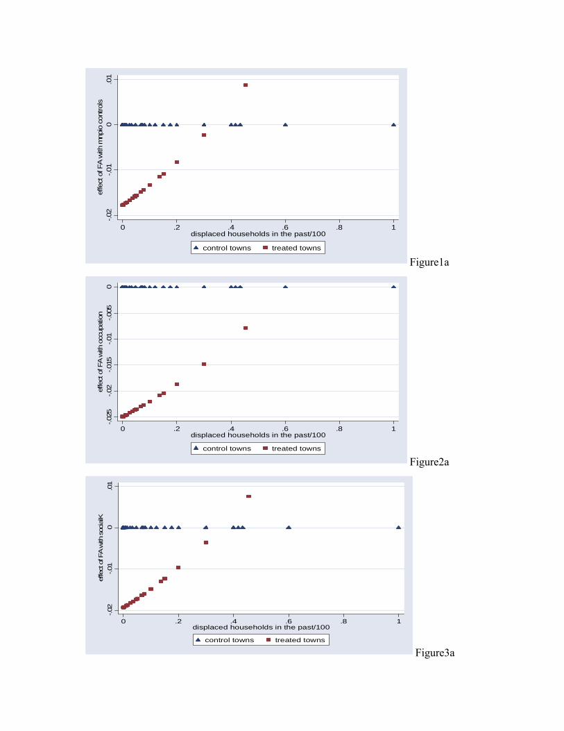
-.02

-.01

0.0

1ef

fect

of F

A w

ith m

npio

con

trols

0 .2 .4 .6 .8 1displaced households in the past/100

control towns treated towns

Figure1a

-.025

-.02

-.015

-.01

-.005

0ef

fect

of F

A w

ith o

ccup

atio

n

0 .2 .4 .6 .8 1displaced households in the past/100

control towns treated towns

Figure2a

-.02

-.01

0.0

1ef

fect

of F

A w

ith s

ocia

lK

0 .2 .4 .6 .8 1displaced households in the past/100

control towns treated towns

Figure3a

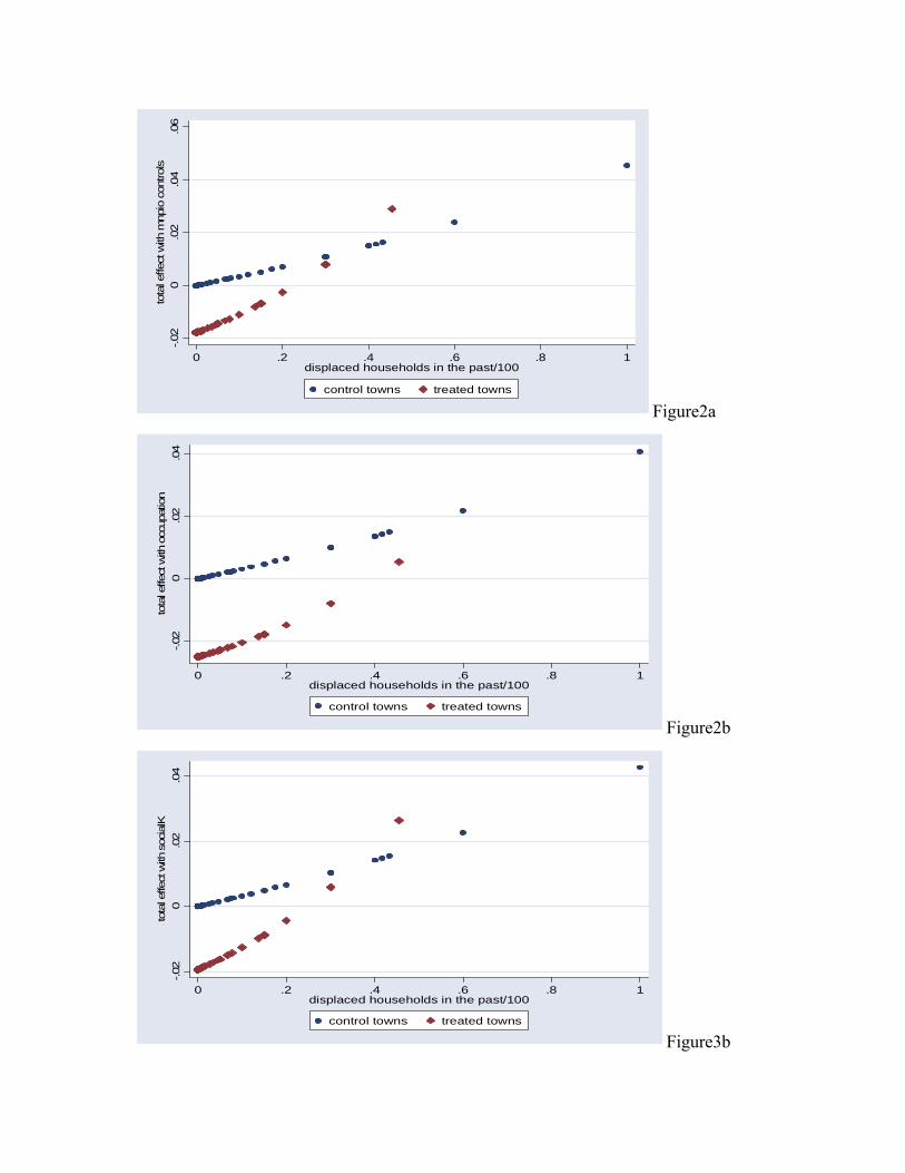
-.02

0.0

2.0

4.0

6to

tal e

ffect

with

mnp

io c

ontro

ls

0 .2 .4 .6 .8 1displaced households in the past/100

control towns treated towns

Figure2a

-.02

0.0

2.0

4to

tal e

ffect

with

occ

upat

ion

0 .2 .4 .6 .8 1displaced households in the past/100

control towns treated towns

Figure2b

-.02

0.0

2.0

4to

tal e

ffect

with

soc

ialK

0 .2 .4 .6 .8 1displaced households in the past/100

control towns treated towns

Figure3b

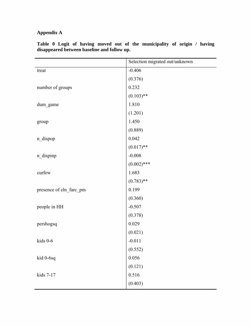
Appendix A Table 0 Logit of having moved out of the municipality of origin / having disappeared between baseline and follow up. Selection migrated out/unknown

treat -0.406

(0.376)

number of groups 0.232

(0.103)**

dum_game 1.810

(1.201)

group 1.450

(0.889)

n_dispop 0.042

(0.017)**

n_dispinp -0.008

(0.002)***

curfew 1.683

(0.783)**

presence of eln_farc_pm 0.199

(0.360)

people in HH -0.507

(0.378)

pershogsq 0.029

(0.021)

kids 0-6 -0.011

(0.552)

kid 0-6sq 0.056

(0.121)

kids 7-17 0.516

(0.403)

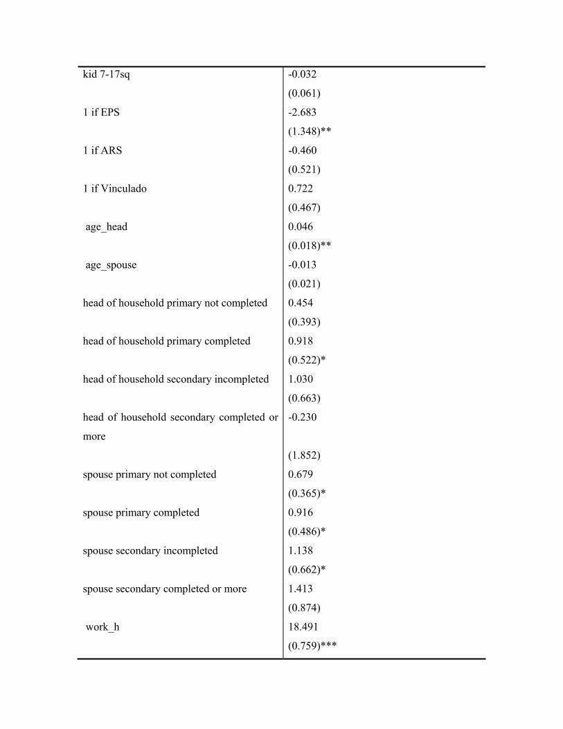
kid 7-17sq -0.032

(0.061)

1 if EPS -2.683

(1.348)**

1 if ARS -0.460

(0.521)

1 if Vinculado 0.722

(0.467)

age_head 0.046

(0.018)**

age_spouse -0.013

(0.021)

head of household primary not completed 0.454

(0.393)

head of household primary completed 0.918

(0.522)*

head of household secondary incompleted 1.030

(0.663)

head of household secondary completed or

more

-0.230

(1.852)

spouse primary not completed 0.679

(0.365)*

spouse primary completed 0.916

(0.486)*

spouse secondary incompleted 1.138

(0.662)*

spouse secondary completed or more 1.413

(0.874)

work_h 18.491

(0.759)***

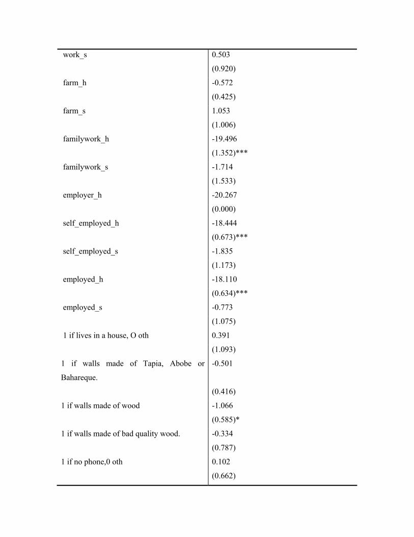
work_s 0.503

(0.920)

farm_h -0.572

(0.425)

farm_s 1.053

(1.006)

familywork_h -19.496

(1.352)***

familywork_s -1.714

(1.533)

employer_h -20.267

(0.000)

self_employed_h -18.444

(0.673)***

self_employed_s -1.835

(1.173)

employed_h -18.110

(0.634)***

employed_s -0.773

(1.075)

1 if lives in a house, O oth 0.391

(1.093)

1 if walls made of Tapia, Abobe or

Bahareque.

-0.501

(0.416)

1 if walls made of wood -1.066

(0.585)*

1 if walls made of bad quality wood. -0.334

(0.787)

1 if no phone,0 oth 0.102

(0.662)

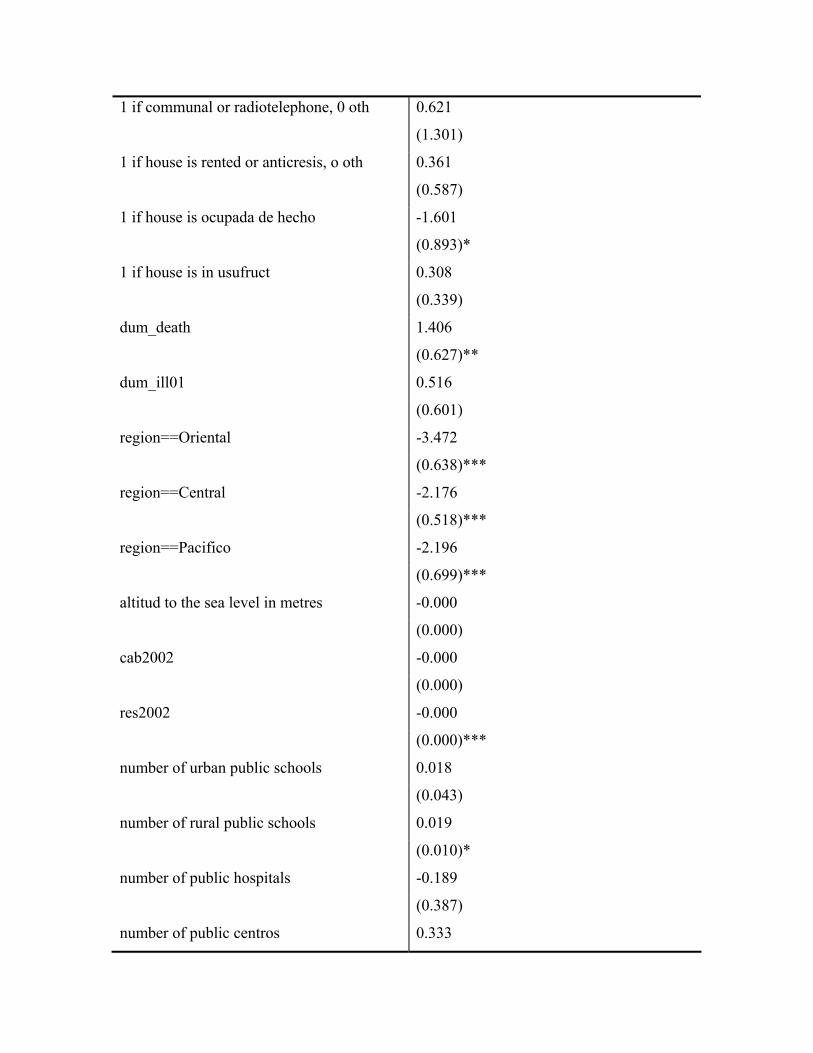
1 if communal or radiotelephone, 0 oth 0.621

(1.301)

1 if house is rented or anticresis, o oth 0.361

(0.587)

1 if house is ocupada de hecho -1.601

(0.893)*

1 if house is in usufruct 0.308

(0.339)

dum_death 1.406

(0.627)**

dum_ill01 0.516

(0.601)

region==Oriental -3.472

(0.638)***

region==Central -2.176

(0.518)***

region==Pacifico -2.196

(0.699)***

altitud to the sea level in metres -0.000

(0.000)

cab2002 -0.000

(0.000)

res2002 -0.000

(0.000)***

number of urban public schools 0.018

(0.043)

number of rural public schools 0.019

(0.010)*

number of public hospitals -0.189

(0.387)

number of public centros 0.333

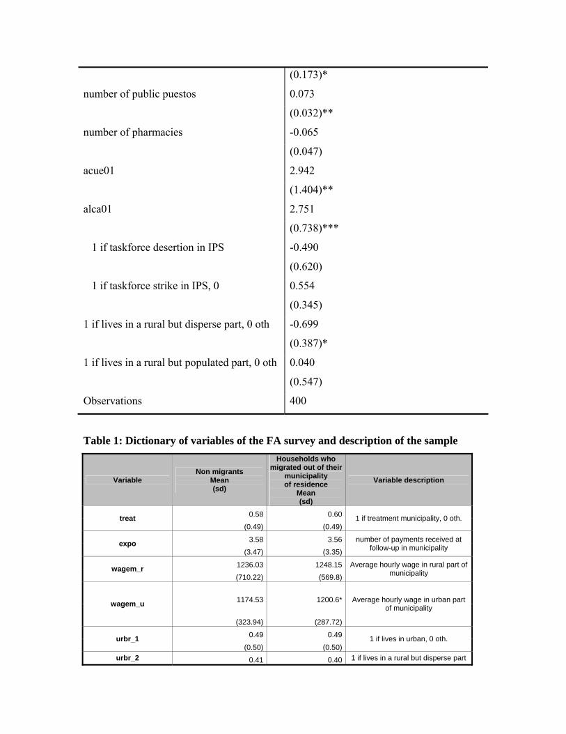
(0.173)*

number of public puestos 0.073

(0.032)**

number of pharmacies -0.065

(0.047)

acue01 2.942

(1.404)**

alca01 2.751

(0.738)***

1 if taskforce desertion in IPS -0.490

(0.620)

1 if taskforce strike in IPS, 0 0.554

(0.345)

1 if lives in a rural but disperse part, 0 oth -0.699

(0.387)*

1 if lives in a rural but populated part, 0 oth 0.040

(0.547)

Observations 400

Table 1: Dictionary of variables of the FA survey and description of the sample

Variable Non migrants

Mean (sd)

Households who migrated out of their

municipality of residence

Mean (sd)

Variable description

0.58 0.60treat (0.49) (0.49)

1 if treatment municipality, 0 oth.

3.58 3.56expo (3.47) (3.35)

number of payments received at follow-up in municipality

1236.03 1248.15wagem_r (710.22) (569.8)

Average hourly wage in rural part of municipality

1174.53 1200.6*wagem_u

(323.94) (287.72)

Average hourly wage in urban part of municipality

0.49 0.49urbr_1 (0.50) (0.50)

1 if lives in urban, 0 oth.

urbr_2 0.41 0.40 1 if lives in a rural but disperse part

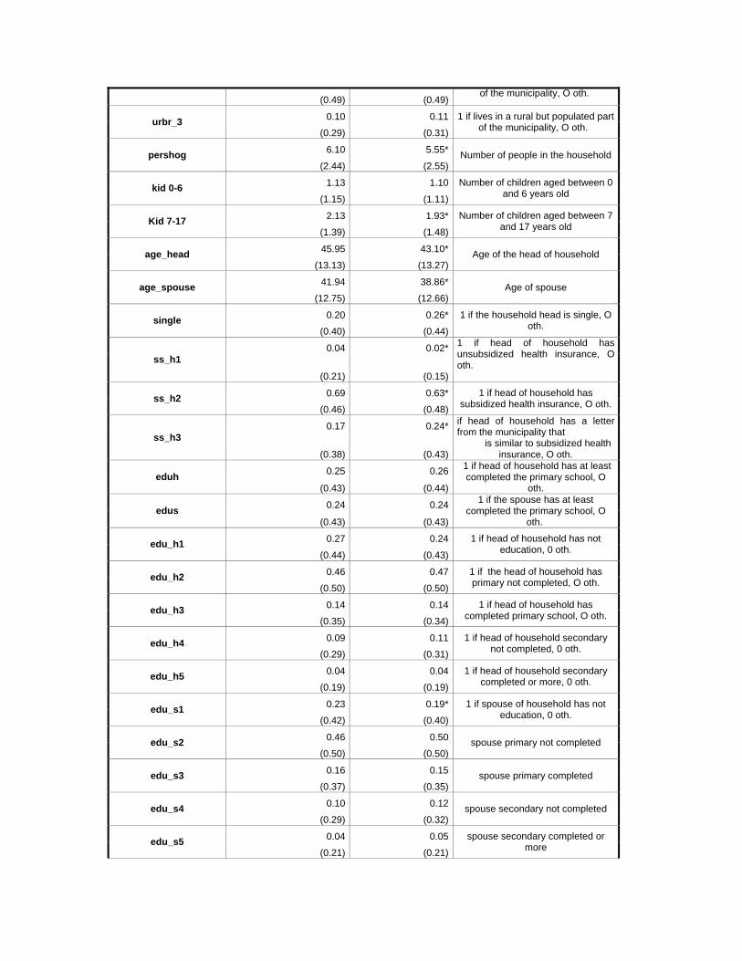
(0.49) (0.49)of the municipality, O oth.

0.10 0.11urbr_3 (0.29) (0.31)

1 if lives in a rural but populated part of the municipality, O oth.

6.10 5.55*pershog (2.44) (2.55)

Number of people in the household

1.13 1.10kid 0-6 (1.15) (1.11)

Number of children aged between 0 and 6 years old

2.13 1.93*Kid 7-17 (1.39) (1.48)

Number of children aged between 7 and 17 years old

45.95 43.10*age_head (13.13) (13.27)

Age of the head of household

41.94 38.86*age_spouse (12.75) (12.66)

Age of spouse

0.20 0.26*single (0.40) (0.44)

1 if the household head is single, O oth.

0.04 0.02*ss_h1

(0.21) (0.15)

1 if head of household has unsubsidized health insurance, O oth.

0.69 0.63*ss_h2 (0.46) (0.48)

1 if head of household has subsidized health insurance, O oth.

0.17 0.24*ss_h3

(0.38) (0.43)

if head of household has a letter from the municipality that is similar to subsidized health

insurance, O oth.

0.25 0.26eduh (0.43) (0.44)

1 if head of household has at least completed the primary school, O

oth.

0.24 0.24edus (0.43) (0.43)

1 if the spouse has at least completed the primary school, O

oth.

0.27 0.24edu_h1 (0.44) (0.43)

1 if head of household has not education, 0 oth.

0.46 0.47edu_h2 (0.50) (0.50)

1 if the head of household has primary not completed, O oth.

0.14 0.14edu_h3 (0.35) (0.34)

1 if head of household has completed primary school, O oth.

0.09 0.11edu_h4 (0.29) (0.31)

1 if head of household secondary not completed, 0 oth.

0.04 0.04edu_h5 (0.19) (0.19)

1 if head of household secondary completed or more, 0 oth.

0.23 0.19*edu_s1 (0.42) (0.40)

1 if spouse of household has not education, 0 oth.

0.46 0.50edu_s2 (0.50) (0.50)

spouse primary not completed

0.16 0.15edu_s3 (0.37) (0.35)

spouse primary completed

0.10 0.12edu_s4 (0.29) (0.32)

spouse secondary not completed

0.04 0.05edu_s5 (0.21) (0.21)

spouse secondary completed or more

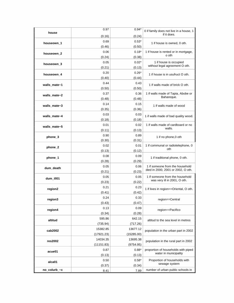
0.97 0.94*house

(0.16) (0.24)

0 if family does not live in a house, 1 if it does.

0.69 0.53*houseown_1 (0.46) (0.50)

1 if house is owned, 0 oth.

0.06 0.18*houseown_2 (0.24) (0.38)

1 if house is rented or in mortgage, o oth

0.05 0.02*houseown_3 (0.21) (0.13)

1 if house is occupied without legal agreement O oth.

0.20 0.26*houseown_4 (0.40) (0.44)

1 if house is in usufruct O oth.

0.44 0.43walls_mate~1 (0.50) (0.50)

1 if walls made of brick O oth.

0.37 0.36walls_mate~2 (0.48) (0.48)

1 if walls made of Tapia, Abobe or Bahareque.

0.14 0.15walls_mate~3 (0.35) (0.36)

1 if walls made of wood

0.03 0.03walls_mate~4 (0.18) (0.18)

1 if walls made of bad quality wood.

0.01 0.02walls_mate~5 (0.11) (0.13)

1 if walls made of cardboard or no walls.

0.90 0.89phone_3 (0.30) (0.31)

1 if no phone,0 oth

0.02 0.01phone_2 (0.13) (0.12)

1 if communal or radiotelephone, 0 oth

0.08 0.09phone_1 (0.28) (0.29)

1 if traditional phone, 0 oth.

0.05 0.06dum_death (0.21) (0.23)

1 if someone from the household died in 2000, 2001 or 2002, O oth.

0.05 0.05dum_ill01 (0.23) (0.22)

1 if someone from the household was very ill in 2001, O oth.

0.21 0.23region2 (0.41) (0.42)

1 if lives in region==Oriental, O oth.

0.24 0.33region3 (0.43) (0.47)

region==Central

0.13 0.09region4 (0.34) (0.28)

region==Pacifico

595.86 642.15altitud (735.94) (717.26)

altitud to the sea level in metres

15382.85 13677.12cab2002 (17921.23) (15285.00)

population in the urban part in 2002

14034.35 13695.38res2002 (11151.83) (9754.95)

population in the rural part in 2002

0.87 0.88*acue01 (0.13) (0.13)

proportion of households with piped water in municipality

0.50 0.58*alca01 (0.37) (0.34)

Proportion of households with sewage system

no_colurb_~c 8.41 7.89 number of urban public schools in

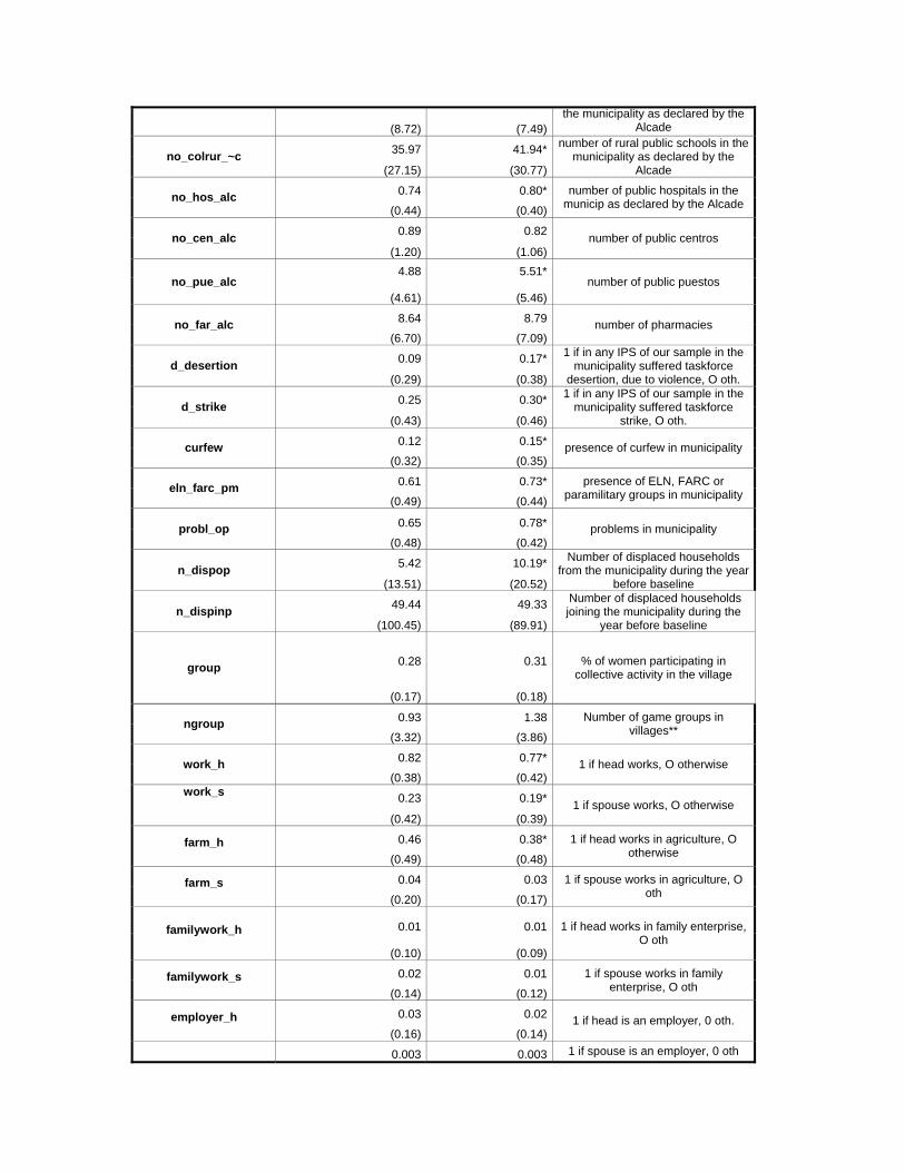
(8.72) (7.49)the municipality as declared by the

Alcade

35.97 41.94*no_colrur_~c (27.15) (30.77)

number of rural public schools in the municipality as declared by the

Alcade

0.74 0.80*no_hos_alc (0.44) (0.40)

number of public hospitals in the municip as declared by the Alcade

0.89 0.82no_cen_alc (1.20) (1.06)

number of public centros

4.88 5.51*no_pue_alc

(4.61) (5.46)number of public puestos

8.64 8.79no_far_alc (6.70) (7.09)

number of pharmacies

0.09 0.17*d_desertion (0.29) (0.38)

1 if in any IPS of our sample in the municipality suffered taskforce

desertion, due to violence, O oth.

0.25 0.30*d_strike (0.43) (0.46)

1 if in any IPS of our sample in the municipality suffered taskforce

strike, O oth.

0.12 0.15*curfew (0.32) (0.35)

presence of curfew in municipality

0.61 0.73*eln_farc_pm (0.49) (0.44)

presence of ELN, FARC or paramilitary groups in municipality

0.65 0.78*probl_op (0.48) (0.42)

problems in municipality

5.42 10.19*n_dispop (13.51) (20.52)

Number of displaced households from the municipality during the year

before baseline

49.44 49.33n_dispinp (100.45) (89.91)

Number of displaced households joining the municipality during the

year before baseline

0.28 0.31group

(0.17) (0.18)

% of women participating in collective activity in the village

0.93 1.38ngroup (3.32) (3.86)

Number of game groups in villages**

0.82 0.77*work_h (0.38) (0.42)

1 if head works, O otherwise

0.23 0.19*work_s (0.42) (0.39)

1 if spouse works, O otherwise

0.46 0.38*farm_h (0.49) (0.48)

1 if head works in agriculture, O otherwise

0.04 0.03farm_s (0.20) (0.17)

1 if spouse works in agriculture, O oth

0.01 0.01familywork_h

(0.10) (0.09)

1 if head works in family enterprise, O oth

0.02 0.01familywork_s (0.14) (0.12)

1 if spouse works in family enterprise, O oth

0.03 0.02employer_h (0.16) (0.14)

1 if head is an employer, 0 oth.

0.003 0.003 1 if spouse is an employer, 0 oth

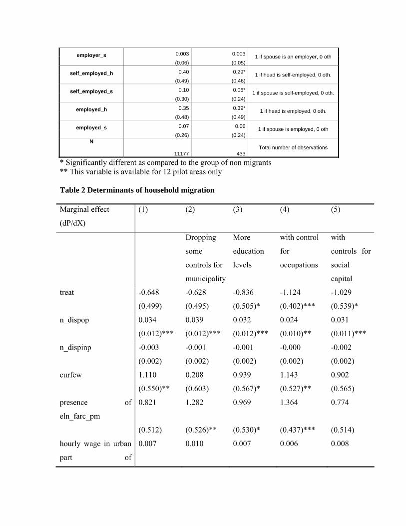
0.003 0.003employer_s (0.06) (0.05)

1 if spouse is an employer, 0 oth

0.40 0.29*self_employed_h (0.49) (0.46)

1 if head is self-employed, 0 oth.

0.10 0.06*self_employed_s (0.30) (0.24)

1 if spouse is self-employed, 0 oth.

0.35 0.39*employed_h (0.48) (0.49)

1 if head is employed, 0 oth.

0.07 0.06employed_s (0.26) (0.24)

1 if spouse is employed, 0 oth

N 11177 433

Total number of observations

* Significantly different as compared to the group of non migrants ** This variable is available for 12 pilot areas only Table 2 Determinants of household migration Marginal effect

(dP/dX)

(1) (2) (3) (4) (5)

Dropping

some

controls for

municipality

More

education

levels

with control

for

occupations

with

controls for

social

capital

treat -0.648 -0.628 -0.836 -1.124 -1.029

(0.499) (0.495) (0.505)* (0.402)*** (0.539)*

n_dispop 0.034 0.039 0.032 0.024 0.031

(0.012)*** (0.012)*** (0.012)*** (0.010)** (0.011)***

n_dispinp -0.003 -0.001 -0.001 -0.000 -0.002

(0.002) (0.002) (0.002) (0.002) (0.002)

curfew 1.110 0.208 0.939 1.143 0.902

(0.550)** (0.603) (0.567)* (0.527)** (0.565)

presence of

eln_farc_pm

0.821 1.282 0.969 1.364 0.774

(0.512) (0.526)** (0.530)* (0.437)*** (0.514)

hourly wage in urban

part of

0.007 0.010 0.007 0.006 0.008

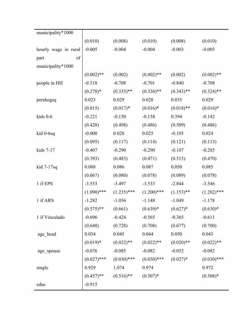
municipality*1000

(0.010) (0.008) (0.010) (0.008) (0.010)

hourly wage in rural

part of

municipality*1000

-0.005 -0.004 -0.004 -0.003 -0.005

(0.002)** (0.002) (0.002)** (0.002) (0.002)**

people in HH -0.518 -0.708 -0.701 -0.840 -0.708

(0.278)* (0.335)** (0.326)** (0.343)** (0.324)**

pershogsq 0.023 0.029 0.028 0.035 0.029

(0.015) (0.017)* (0.016)* (0.018)** (0.016)*

kids 0-6 -0.221 -0.150 -0.138 0.394 -0.142

(0.428) (0.498) (0.486) (0.509) (0.486)

kid 0-6sq -0.000 0.028 0.025 -0.105 0.024

(0.095) (0.117) (0.114) (0.121) (0.113)

kids 7-17 -0.407 -0.290 -0.290 -0.107 -0.285

(0.393) (0.483) (0.471) (0.513) (0.470)

kid 7-17sq 0.088 0.086 0.087 0.050 0.085

(0.067) (0.080) (0.078) (0.089) (0.078)

1 if EPS -3.553 -3.497 -3.533 -2.844 -3.546

(1.090)*** (1.235)*** (1.200)*** (1.153)** (1.202)***

1 if ARS -1.282 -1.056 -1.148 -1.049 -1.178

(0.575)** (0.661) (0.639)* (0.627)* (0.630)*

1 if Vinculado -0.696 -0.424 -0.565 -0.365 -0.611

(0.648) (0.728) (0.708) (0.677) (0.700)

age_head 0.034 0.045 0.044 0.050 0.043

(0.019)* (0.022)** (0.022)** (0.020)** (0.022)**

age_spouse -0.076 -0.085 -0.082 -0.052 -0.082

(0.027)*** (0.030)*** (0.030)*** (0.027)* (0.030)***

single 0.929 1.074 0.974 0.972

(0.457)** (0.516)** (0.507)* (0.508)*

edus -0.915

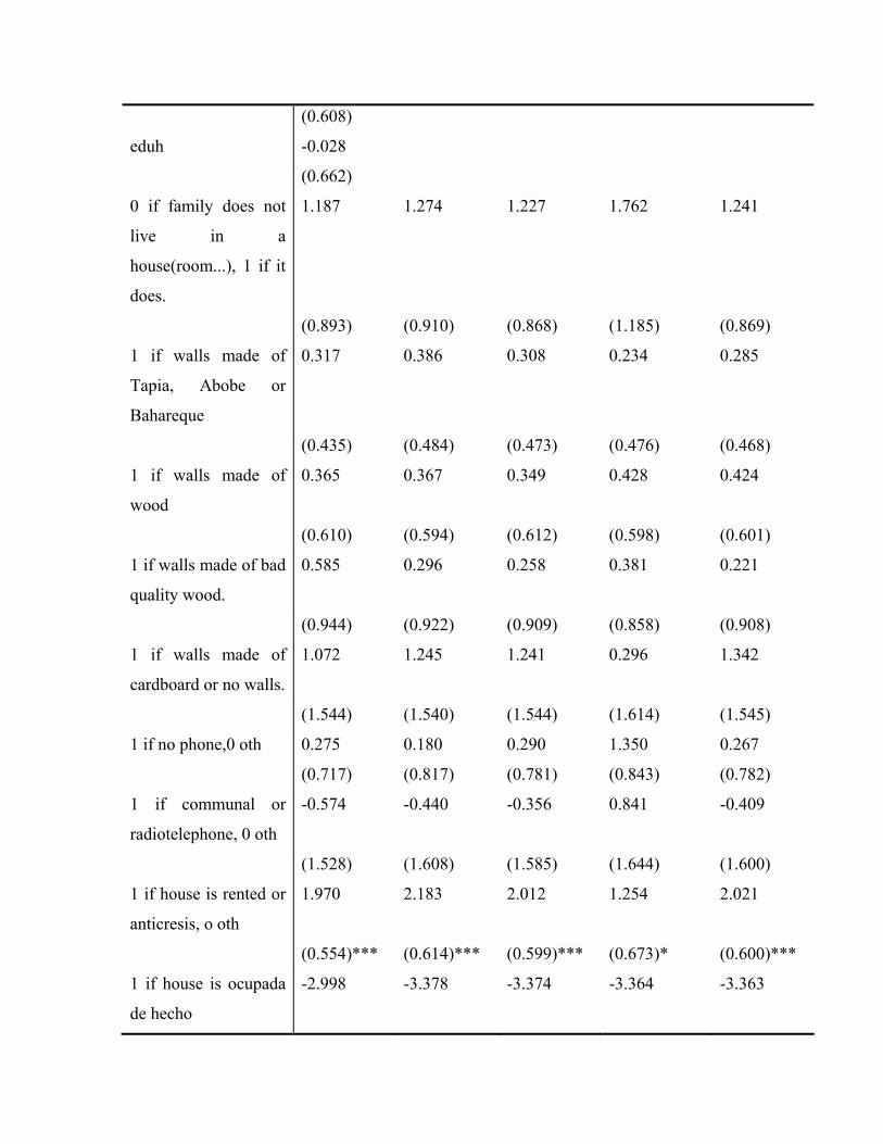
(0.608)

eduh -0.028

(0.662)

0 if family does not

live in a

house(room...), 1 if it

does.

1.187 1.274 1.227 1.762 1.241

(0.893) (0.910) (0.868) (1.185) (0.869)

1 if walls made of

Tapia, Abobe or

Bahareque

0.317 0.386 0.308 0.234 0.285

(0.435) (0.484) (0.473) (0.476) (0.468)

1 if walls made of

wood

0.365 0.367 0.349 0.428 0.424

(0.610) (0.594) (0.612) (0.598) (0.601)

1 if walls made of bad

quality wood.

0.585 0.296 0.258 0.381 0.221

(0.944) (0.922) (0.909) (0.858) (0.908)

1 if walls made of

cardboard or no walls.

1.072 1.245 1.241 0.296 1.342

(1.544) (1.540) (1.544) (1.614) (1.545)

1 if no phone,0 oth 0.275 0.180 0.290 1.350 0.267

(0.717) (0.817) (0.781) (0.843) (0.782)

1 if communal or

radiotelephone, 0 oth

-0.574 -0.440 -0.356 0.841 -0.409

(1.528) (1.608) (1.585) (1.644) (1.600)

1 if house is rented or

anticresis, o oth

1.970 2.183 2.012 1.254 2.021

(0.554)*** (0.614)*** (0.599)*** (0.673)* (0.600)***

1 if house is ocupada

de hecho

-2.998 -3.378 -3.374 -3.364 -3.363

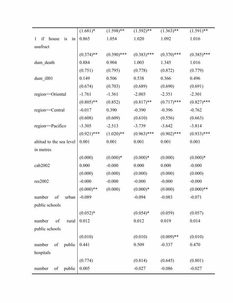
(1.681)* (1.598)** (1.592)** (1.363)** (1.591)**

1 if house is in

usufruct

0.865 1.054 1.020 1.092 1.016

(0.374)** (0.390)*** (0.383)*** (0.370)*** (0.385)***

dum_death 0.884 0.904 1.003 1.345 1.016

(0.751) (0.795) (0.778) (0.872) (0.779)

dum_ill01 0.149 0.506 0.538 0.366 0.496

(0.674) (0.703) (0.689) (0.690) (0.691)

region==Oriental -1.761 -1.361 -2.003 -2.351 -2.301

(0.805)** (0.852) (0.817)** (0.717)*** (0.827)***

region==Central -0.017 0.390 -0.390 -0.396 -0.762

(0.608) (0.609) (0.610) (0.556) (0.663)

region==Pacifico -3.305 -2.513 -3.739 -3.642 -3.814

(0.921)*** (1.020)** (0.963)*** (0.902)*** (0.933)***

altitud to the sea level

in metres

0.001 0.001 0.001 0.001 0.001

(0.000) (0.000)* (0.000)* (0.000) (0.000)*

cab2002 0.000 -0.000 0.000 0.000 -0.000

(0.000) (0.000) (0.000) (0.000) (0.000)

res2002 -0.000 -0.000 -0.000 -0.000 -0.000

(0.000)** (0.000) (0.000)* (0.000) (0.000)**

number of urban

public schools

-0.089 -0.094 -0.083 -0.071

(0.052)* (0.054)* (0.059) (0.057)

number of rural

public schools

0.012 0.012 0.019 0.014

(0.010) (0.010) (0.009)** (0.010)

number of public

hospitals

0.441 0.509 -0.337 0.470

(0.774) (0.814) (0.645) (0.801)

number of public 0.005 -0.027 -0.086 -0.027

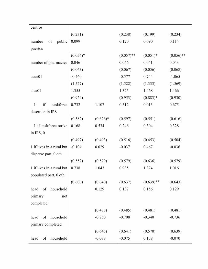
centros

(0.231) (0.238) (0.199) (0.234)

number of public

puestos

0.099 0.120 0.090 0.114

(0.054)* (0.057)** (0.051)* (0.056)**

number of pharmacies 0.046 0.046 0.041 0.043

(0.063) (0.067) (0.056) (0.068)

acue01 -0.460 -0.577 0.744 -1.065

(1.527) (1.522) (1.333) (1.569)

alca01 1.355 1.325 1.468 1.466

(0.924) (0.953) (0.883)* (0.930)

1 if taskforce

desertion in IPS

0.732 1.107 0.512 0.013 0.675

(0.582) (0.626)* (0.597) (0.551) (0.616)

1 if taskforce strike

in IPS, 0

0.168 0.534 0.246 0.304 0.328

(0.497) (0.493) (0.516) (0.453) (0.504)

1 if lives in a rural but

disperse part, 0 oth

-0.104 0.029 -0.037 0.467 -0.036

(0.552) (0.579) (0.579) (0.636) (0.579)

1 if lives in a rural but

populated part, 0 oth

0.738 1.043 0.935 1.374 1.016

(0.606) (0.640) (0.637) (0.639)** (0.643)

head of household

primary not

completed

0.129 0.137 0.156 0.129

(0.488) (0.485) (0.481) (0.481)

head of household

primary completed

-0.750 -0.708 -0.340 -0.736

(0.645) (0.641) (0.570) (0.639)

head of household -0.088 -0.075 0.138 -0.070

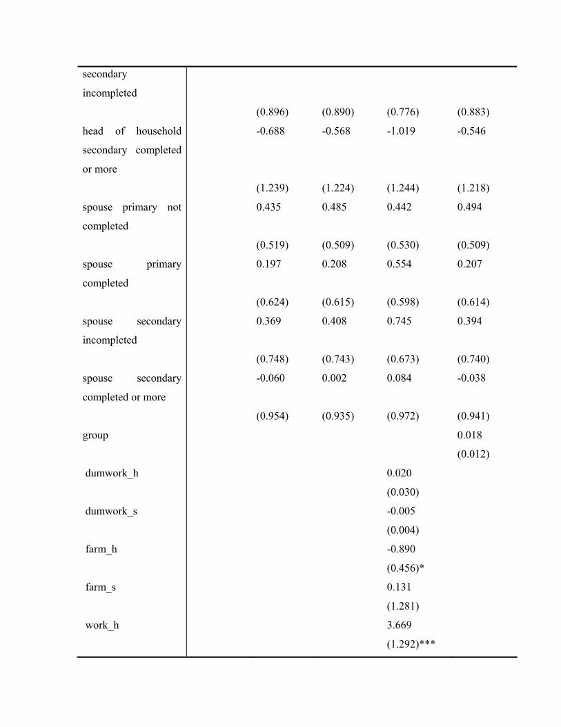
secondary

incompleted

(0.896) (0.890) (0.776) (0.883)

head of household

secondary completed

or more

-0.688 -0.568 -1.019 -0.546

(1.239) (1.224) (1.244) (1.218)

spouse primary not

completed

0.435 0.485 0.442 0.494

(0.519) (0.509) (0.530) (0.509)

spouse primary

completed

0.197 0.208 0.554 0.207

(0.624) (0.615) (0.598) (0.614)

spouse secondary

incompleted

0.369 0.408 0.745 0.394

(0.748) (0.743) (0.673) (0.740)

spouse secondary

completed or more

-0.060 0.002 0.084 -0.038

(0.954) (0.935) (0.972) (0.941)

group 0.018

(0.012)

dumwork_h 0.020

(0.030)

dumwork_s -0.005

(0.004)

farm_h -0.890

(0.456)*

farm_s 0.131

(1.281)

work_h 3.669

(1.292)***

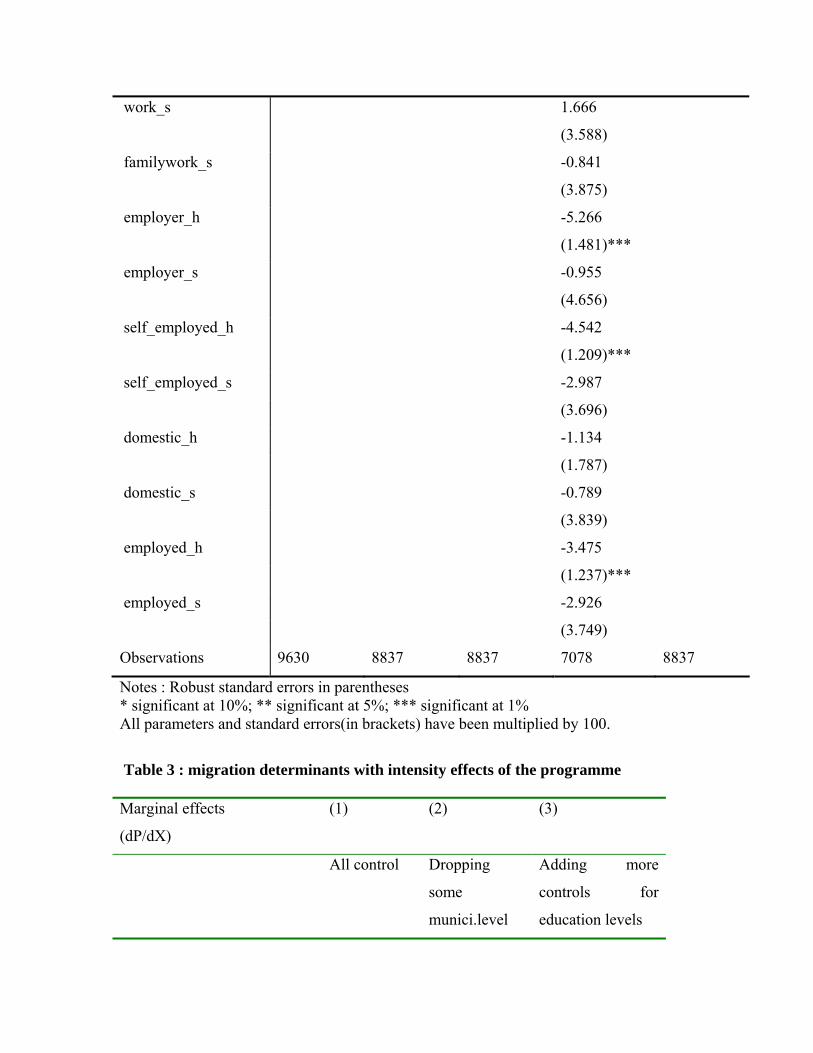
work_s 1.666

(3.588)

familywork_s -0.841

(3.875)

employer_h -5.266

(1.481)***

employer_s -0.955

(4.656)

self_employed_h -4.542

(1.209)***

self_employed_s -2.987

(3.696)

domestic_h -1.134

(1.787)

domestic_s -0.789

(3.839)

employed_h -3.475

(1.237)***

employed_s -2.926

(3.749)

Observations 9630 8837 8837 7078 8837

Notes : Robust standard errors in parentheses * significant at 10%; ** significant at 5%; *** significant at 1% All parameters and standard errors(in brackets) have been multiplied by 100.

Table 3 : migration determinants with intensity effects of the programme Marginal effects

(dP/dX)

(1) (2) (3)

All control Dropping

some

munici.level

Adding more

controls for

education levels

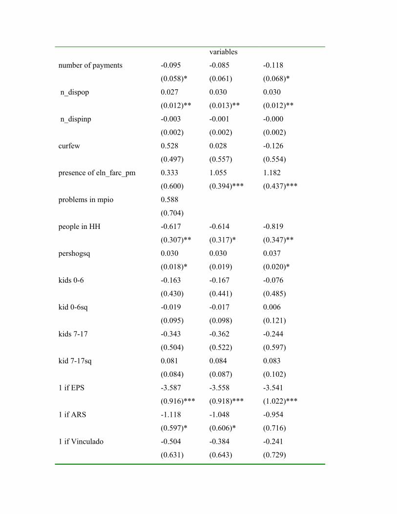
variables

number of payments -0.095 -0.085 -0.118

(0.058)* (0.061) (0.068)*

n_dispop 0.027 0.030 0.030

(0.012)** (0.013)** (0.012)**

n_dispinp -0.003 -0.001 -0.000

(0.002) (0.002) (0.002)

curfew 0.528 0.028 -0.126

(0.497) (0.557) (0.554)

presence of eln_farc_pm 0.333 1.055 1.182

(0.600) (0.394)*** (0.437)***

problems in mpio 0.588

(0.704)

people in HH -0.617 -0.614 -0.819

(0.307)** (0.317)* (0.347)**

pershogsq 0.030 0.030 0.037

(0.018)* (0.019) (0.020)*

kids 0-6 -0.163 -0.167 -0.076

(0.430) (0.441) (0.485)

kid 0-6sq -0.019 -0.017 0.006

(0.095) (0.098) (0.121)

kids 7-17 -0.343 -0.362 -0.244

(0.504) (0.522) (0.597)

kid 7-17sq 0.081 0.084 0.083

(0.084) (0.087) (0.102)

1 if EPS -3.587 -3.558 -3.541

(0.916)*** (0.918)*** (1.022)***

1 if ARS -1.118 -1.048 -0.954

(0.597)* (0.606)* (0.716)

1 if Vinculado -0.504 -0.384 -0.241

(0.631) (0.643) (0.729)

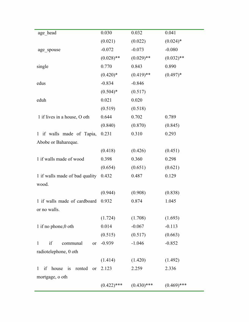
age_head 0.030 0.032 0.041

(0.021) (0.022) (0.024)*

age_spouse -0.072 -0.073 -0.080

(0.028)** (0.029)** (0.032)**

single 0.770 0.843 0.890

(0.420)* (0.419)** (0.497)*

edus -0.834 -0.846

(0.504)* (0.517)

eduh 0.021 0.020

(0.519) (0.518)

1 if lives in a house, O oth 0.644 0.702 0.789

(0.840) (0.870) (0.845)

1 if walls made of Tapia,

Abobe or Bahareque.

0.231 0.310 0.293

(0.418) (0.426) (0.451)

1 if walls made of wood 0.398 0.360 0.298

(0.654) (0.651) (0.621)

1 if walls made of bad quality

wood.

0.432 0.487 0.129

(0.944) (0.908) (0.838)

1 if walls made of cardboard

or no walls.

0.932 0.874 1.045

(1.724) (1.708) (1.693)

1 if no phone,0 oth 0.014 -0.067 -0.113

(0.515) (0.517) (0.663)

1 if communal or

radiotelephone, 0 oth

-0.939 -1.046 -0.852

(1.414) (1.420) (1.492)

1 if house is rented or

mortgage, o oth

2.123 2.259 2.336

(0.422)*** (0.430)*** (0.469)***

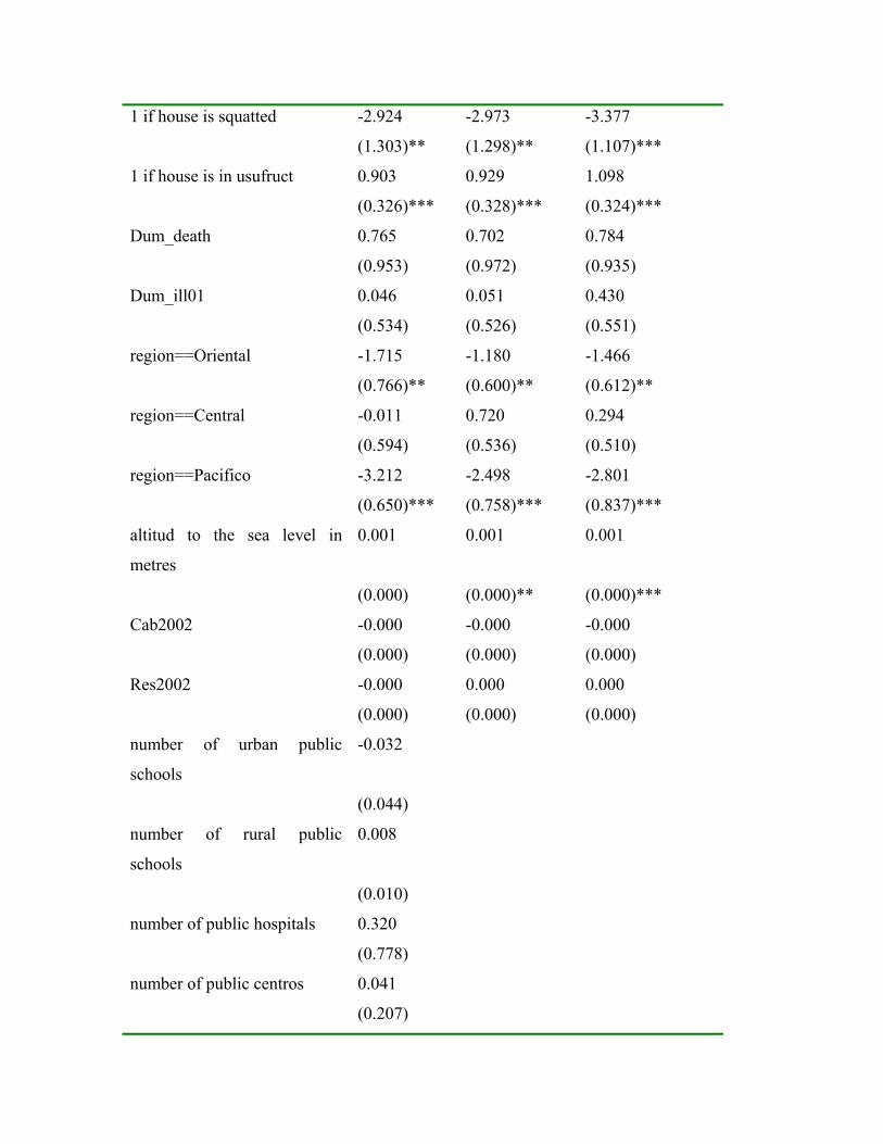
1 if house is squatted -2.924 -2.973 -3.377

(1.303)** (1.298)** (1.107)***

1 if house is in usufruct 0.903 0.929 1.098

(0.326)*** (0.328)*** (0.324)***

Dum_death 0.765 0.702 0.784

(0.953) (0.972) (0.935)

Dum_ill01 0.046 0.051 0.430

(0.534) (0.526) (0.551)

region==Oriental -1.715 -1.180 -1.466

(0.766)** (0.600)** (0.612)**

region==Central -0.011 0.720 0.294

(0.594) (0.536) (0.510)

region==Pacifico -3.212 -2.498 -2.801

(0.650)*** (0.758)*** (0.837)***

altitud to the sea level in

metres

0.001 0.001 0.001

(0.000) (0.000)** (0.000)***

Cab2002 -0.000 -0.000 -0.000

(0.000) (0.000) (0.000)

Res2002 -0.000 0.000 0.000

(0.000) (0.000) (0.000)

number of urban public

schools

-0.032

(0.044)

number of rural public

schools

0.008

(0.010)

number of public hospitals 0.320

(0.778)

number of public centros 0.041

(0.207)

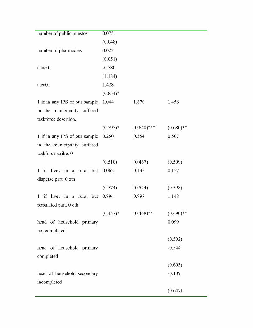
number of public puestos 0.075

(0.048)

number of pharmacies 0.023

(0.051)

acue01 -0.580

(1.184)

alca01 1.428

(0.854)*

1 if in any IPS of our sample

in the municipality suffered

taskforce desertion,

1.044 1.670 1.458

(0.595)* (0.640)*** (0.680)**

1 if in any IPS of our sample

in the municipality suffered

taskforce strike, 0

0.250 0.354 0.507

(0.510) (0.467) (0.509)

1 if lives in a rural but

disperse part, 0 oth

0.062 0.135 0.157

(0.574) (0.574) (0.598)

1 if lives in a rural but

populated part, 0 oth

0.894 0.997 1.148

(0.457)* (0.468)** (0.490)**

head of household primary

not completed

0.099

(0.502)

head of household primary

completed

-0.544

(0.603)

head of household secondary

incompleted

-0.109

(0.647)

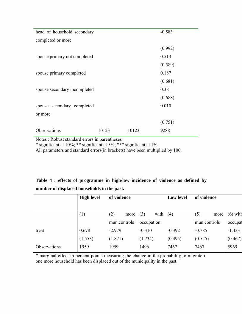
head of household secondary

completed or more

-0.583

(0.992)

spouse primary not completed 0.513

(0.589)

spouse primary completed 0.187

(0.681)

spouse secondary incompleted 0.381

(0.688)

spouse secondary completed

or more

0.010

(0.751)

Observations 10123 10123 9288

Notes : Robust standard errors in parentheses * significant at 10%; ** significant at 5%; *** significant at 1% All parameters and standard errors(in brackets) have been multiplied by 100.

Table 4 : effects of programme in high/low incidence of violence as defined by

number of displaced households in the past.

High level

of violence Low level of violence

(1) (2) more

mun.controls

(3) with

occupation

(4) (5) more

mun.controls

(6) with

occupat

treat 0.678 -2.979 -0.310 -0.392 -0.785 -1.433

(1.553) (1.871) (1.734) (0.495) (0.525) (0.467)*

Observations 1959 1959 1496 7467 7467 5969

* marginal effect in percent points measuring the change in the probability to migrate if one more household has been displaced out of the municipality in the past.

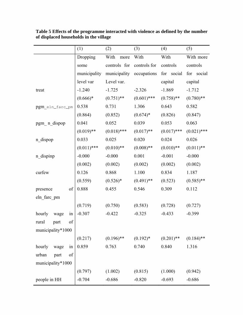
Table 5 Effects of the programme interacted with violence as defined by the number of displaced households in the village (1) (2) (3) (4) (5)

Dropping

some

municipality

level var

With more

controls for

municipality

Level var.

With

controls for

occupations

With

controls

for social

capital

With more

controls

for social

capital

treat -1.240 -1.725 -2.326 -1.869 -1.712

(0.666)* (0.751)** (0.601)*** (0.758)** (0.780)**

pgm_eln_farc_pm 0.538 0.731 1.306 0.643 0.582

(0.864) (0.852) (0.674)* (0.826) (0.847)

pgm_ n_dispop 0.041 0.052 0.039 0.053 0.063

(0.019)** (0.018)*** (0.017)** (0.017)*** (0.021)***

n_dispop 0.033 0.025 0.020 0.024 0.026

(0.011)*** (0.010)** (0.008)** (0.010)** (0.011)**

n_dispinp -0.000 -0.000 0.001 -0.001 -0.000

(0.002) (0.002) (0.002) (0.002) (0.002)

curfew 0.126 0.868 1.100 0.834 1.187

(0.559) (0.526)* (0.491)** (0.523) (0.585)**

presence of

eln_farc_pm

0.888 0.455 0.546 0.309 0.112

(0.719) (0.750) (0.583) (0.728) (0.727)

hourly wage in

rural part of

municipality*1000

-0.307 -0.422 -0.325 -0.433 -0.399

(0.217) (0.196)** (0.192)* (0.201)** (0.184)**

hourly wage in

urban part of

municipality*1000

0.859 0.763 0.740 0.840 1.316

(0.797) (1.002) (0.815) (1.000) (0.942)

people in HH -0.704 -0.686 -0.820 -0.693 -0.686

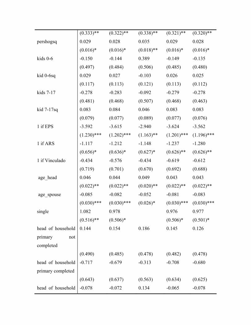
(0.333)** (0.322)** (0.338)** (0.321)** (0.320)**

pershogsq 0.029 0.028 0.035 0.029 0.028

(0.016)* (0.016)* (0.018)** (0.016)* (0.016)*

kids 0-6 -0.150 -0.144 0.389 -0.149 -0.135

(0.497) (0.484) (0.506) (0.485) (0.480)

kid 0-6sq 0.029 0.027 -0.103 0.026 0.025

(0.117) (0.113) (0.121) (0.113) (0.112)

kids 7-17 -0.278 -0.283 -0.092 -0.279 -0.278

(0.481) (0.468) (0.507) (0.468) (0.463)

kid 7-17sq 0.083 0.084 0.046 0.083 0.083

(0.079) (0.077) (0.089) (0.077) (0.076)

1 if EPS -3.592 -3.615 -2.940 -3.624 -3.562

(1.230)*** (1.202)*** (1.163)** (1.201)*** (1.196)***

1 if ARS -1.117 -1.212 -1.148 -1.237 -1.280

(0.656)* (0.636)* (0.627)* (0.626)** (0.626)**

1 if Vinculado -0.434 -0.576 -0.434 -0.619 -0.612

(0.719) (0.701) (0.670) (0.692) (0.688)

age_head 0.046 0.044 0.049 0.043 0.043

(0.022)** (0.022)** (0.020)** (0.022)** (0.022)**

age_spouse -0.085 -0.082 -0.052 -0.081 -0.083

(0.030)*** (0.030)*** (0.026)* (0.030)*** (0.030)***

single 1.082 0.978 0.976 0.977

(0.516)** (0.506)* (0.506)* (0.501)*

head of household

primary not

completed

0.144 0.154 0.186 0.145 0.126

(0.490) (0.485) (0.478) (0.482) (0.478)

head of household

primary completed

-0.717 -0.679 -0.313 -0.708 -0.680

(0.643) (0.637) (0.563) (0.634) (0.625)

head of household -0.078 -0.072 0.134 -0.065 -0.078

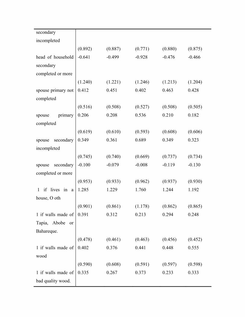
secondary

incompleted

(0.892) (0.887) (0.771) (0.880) (0.875)

head of household

secondary

completed or more

-0.641 -0.499 -0.928 -0.476 -0.466

(1.240) (1.221) (1.246) (1.213) (1.204)

spouse primary not

completed

0.412 0.451 0.402 0.463 0.428

(0.516) (0.508) (0.527) (0.508) (0.505)

spouse primary

completed

0.206 0.208 0.536 0.210 0.182

(0.619) (0.610) (0.593) (0.608) (0.606)

spouse secondary

incompleted

0.349 0.361 0.689 0.349 0.323

(0.745) (0.740) (0.669) (0.737) (0.734)

spouse secondary

completed or more

-0.100 -0.079 -0.008 -0.119 -0.130

(0.953) (0.933) (0.962) (0.937) (0.930)

1 if lives in a

house, O oth

1.285 1.229 1.760 1.244 1.192

(0.901) (0.861) (1.178) (0.862) (0.865)

1 if walls made of

Tapia, Abobe or

Bahareque.

0.391 0.312 0.213 0.294 0.248

(0.478) (0.461) (0.463) (0.456) (0.452)

1 if walls made of

wood

0.402 0.376 0.441 0.448 0.555

(0.590) (0.608) (0.591) (0.597) (0.598)

1 if walls made of

bad quality wood.

0.335 0.267 0.373 0.233 0.333

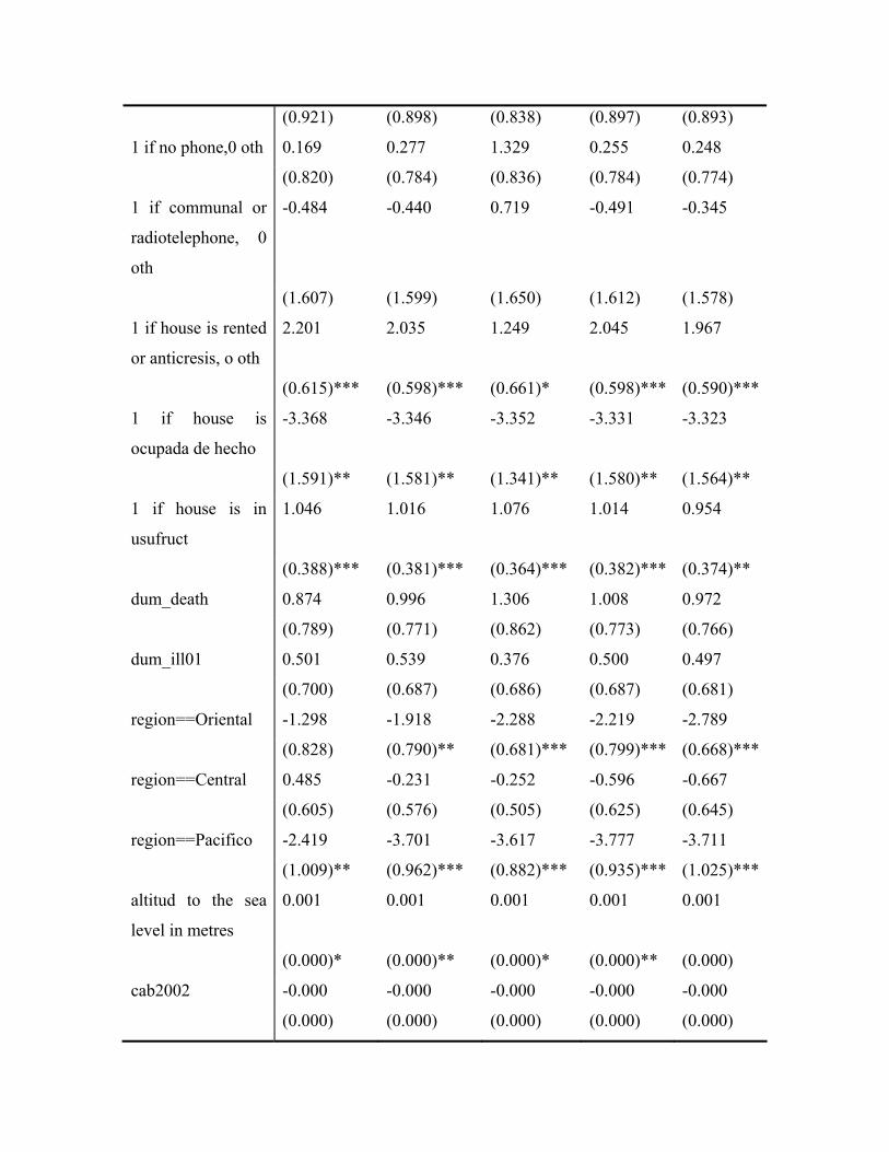
(0.921) (0.898) (0.838) (0.897) (0.893)

1 if no phone,0 oth 0.169 0.277 1.329 0.255 0.248

(0.820) (0.784) (0.836) (0.784) (0.774)

1 if communal or

radiotelephone, 0

oth

-0.484 -0.440 0.719 -0.491 -0.345

(1.607) (1.599) (1.650) (1.612) (1.578)

1 if house is rented

or anticresis, o oth

2.201 2.035 1.249 2.045 1.967

(0.615)*** (0.598)*** (0.661)* (0.598)*** (0.590)***

1 if house is

ocupada de hecho

-3.368 -3.346 -3.352 -3.331 -3.323

(1.591)** (1.581)** (1.341)** (1.580)** (1.564)**

1 if house is in

usufruct

1.046 1.016 1.076 1.014 0.954

(0.388)*** (0.381)*** (0.364)*** (0.382)*** (0.374)**

dum_death 0.874 0.996 1.306 1.008 0.972

(0.789) (0.771) (0.862) (0.773) (0.766)

dum_ill01 0.501 0.539 0.376 0.500 0.497

(0.700) (0.687) (0.686) (0.687) (0.681)

region==Oriental -1.298 -1.918 -2.288 -2.219 -2.789

(0.828) (0.790)** (0.681)*** (0.799)*** (0.668)***

region==Central 0.485 -0.231 -0.252 -0.596 -0.667

(0.605) (0.576) (0.505) (0.625) (0.645)

region==Pacifico -2.419 -3.701 -3.617 -3.777 -3.711

(1.009)** (0.962)*** (0.882)*** (0.935)*** (1.025)***

altitud to the sea

level in metres

0.001 0.001 0.001 0.001 0.001

(0.000)* (0.000)** (0.000)* (0.000)** (0.000)

cab2002 -0.000 -0.000 -0.000 -0.000 -0.000

(0.000) (0.000) (0.000) (0.000) (0.000)

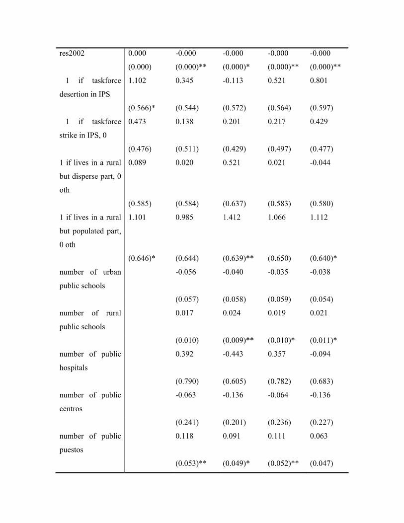
res2002 0.000 -0.000 -0.000 -0.000 -0.000

(0.000) (0.000)** (0.000)* (0.000)** (0.000)**

1 if taskforce

desertion in IPS

1.102 0.345 -0.113 0.521 0.801

(0.566)* (0.544) (0.572) (0.564) (0.597)

1 if taskforce

strike in IPS, 0

0.473 0.138 0.201 0.217 0.429

(0.476) (0.511) (0.429) (0.497) (0.477)

1 if lives in a rural

but disperse part, 0

oth

0.089 0.020 0.521 0.021 -0.044

(0.585) (0.584) (0.637) (0.583) (0.580)

1 if lives in a rural

but populated part,

0 oth

1.101 0.985 1.412 1.066 1.112

(0.646)* (0.644) (0.639)** (0.650) (0.640)*

number of urban

public schools

-0.056 -0.040 -0.035 -0.038

(0.057) (0.058) (0.059) (0.054)

number of rural

public schools

0.017 0.024 0.019 0.021

(0.010) (0.009)** (0.010)* (0.011)*

number of public

hospitals

0.392 -0.443 0.357 -0.094

(0.790) (0.605) (0.782) (0.683)

number of public

centros

-0.063 -0.136 -0.064 -0.136

(0.241) (0.201) (0.236) (0.227)

number of public

puestos

0.118 0.091 0.111 0.063

(0.053)** (0.049)* (0.052)** (0.047)

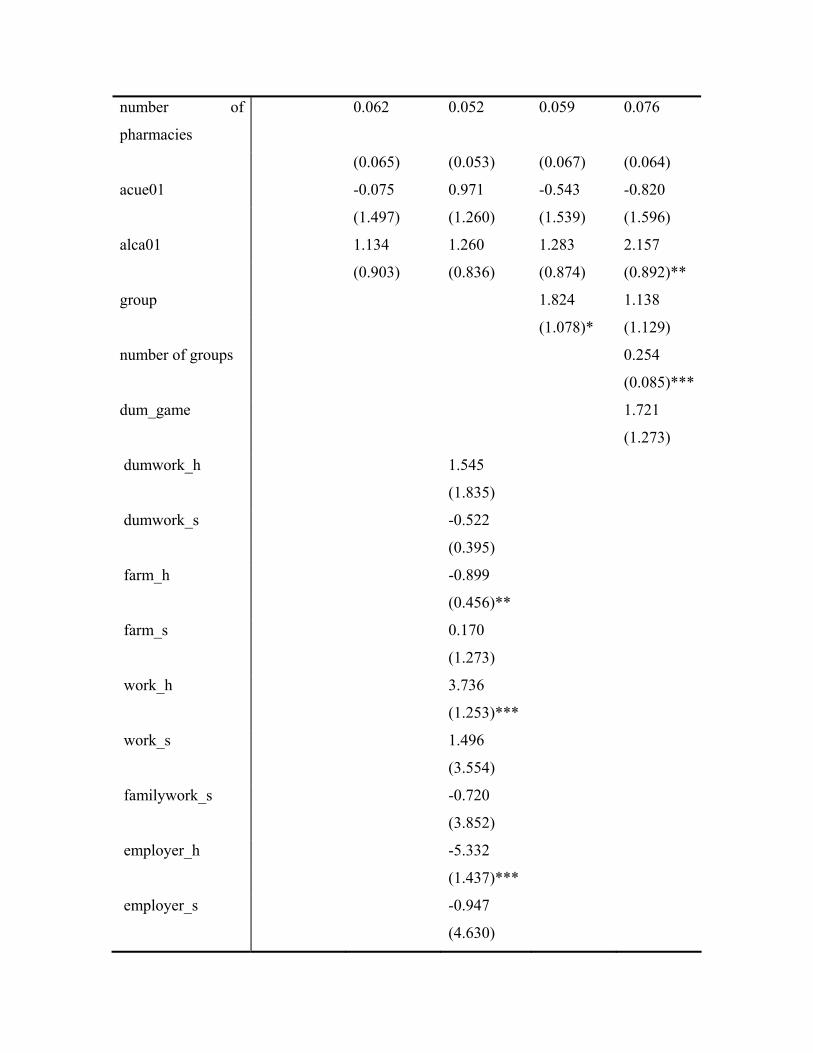
number of

pharmacies

0.062 0.052 0.059 0.076

(0.065) (0.053) (0.067) (0.064)

acue01 -0.075 0.971 -0.543 -0.820

(1.497) (1.260) (1.539) (1.596)

alca01 1.134 1.260 1.283 2.157

(0.903) (0.836) (0.874) (0.892)**

group 1.824 1.138

(1.078)* (1.129)

number of groups 0.254

(0.085)***

dum_game 1.721

(1.273)

dumwork_h 1.545

(1.835)

dumwork_s -0.522

(0.395)

farm_h -0.899

(0.456)**

farm_s 0.170

(1.273)

work_h 3.736

(1.253)***

work_s 1.496

(3.554)

familywork_s -0.720

(3.852)

employer_h -5.332

(1.437)***

employer_s -0.947

(4.630)

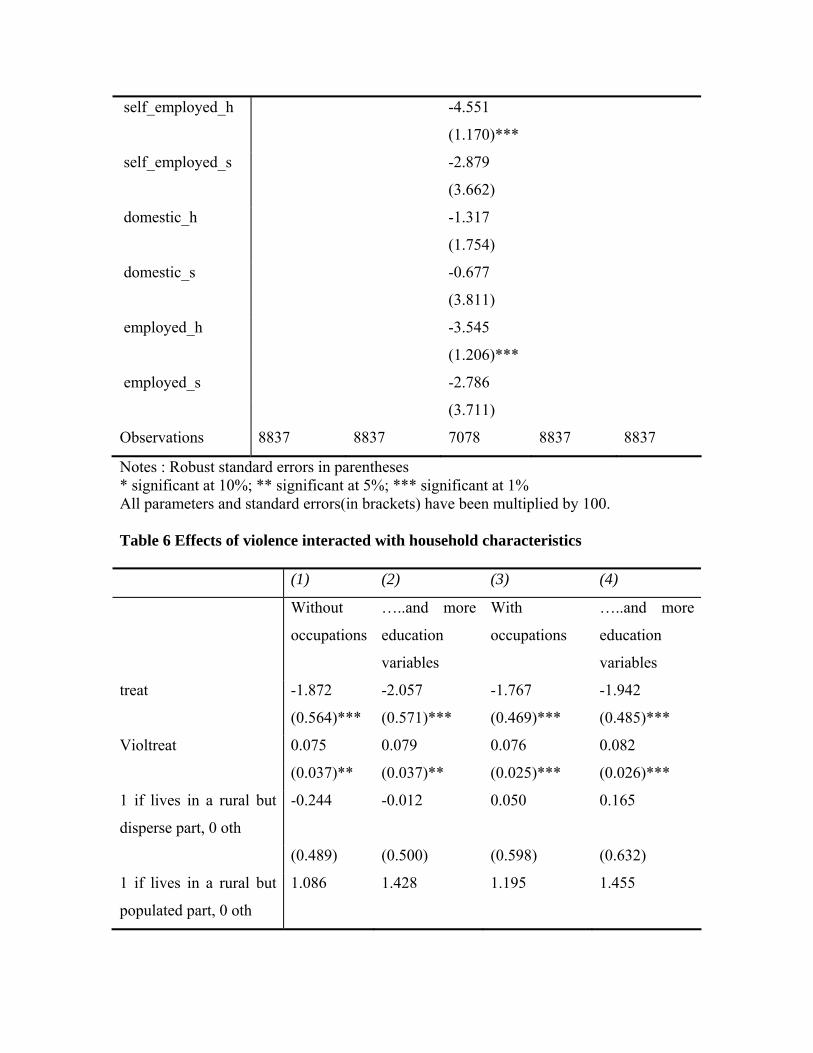
self_employed_h -4.551

(1.170)***

self_employed_s -2.879

(3.662)

domestic_h -1.317

(1.754)

domestic_s -0.677

(3.811)

employed_h -3.545

(1.206)***

employed_s -2.786

(3.711)

Observations 8837 8837 7078 8837 8837

Notes : Robust standard errors in parentheses * significant at 10%; ** significant at 5%; *** significant at 1% All parameters and standard errors(in brackets) have been multiplied by 100. Table 6 Effects of violence interacted with household characteristics (1) (2) (3) (4)

Without

occupations

…..and more

education

variables

With

occupations

…..and more

education

variables

treat -1.872 -2.057 -1.767 -1.942

(0.564)*** (0.571)*** (0.469)*** (0.485)***

Violtreat 0.075 0.079 0.076 0.082

(0.037)** (0.037)** (0.025)*** (0.026)***

1 if lives in a rural but

disperse part, 0 oth

-0.244 -0.012 0.050 0.165

(0.489) (0.500) (0.598) (0.632)

1 if lives in a rural but

populated part, 0 oth

1.086 1.428 1.195 1.455

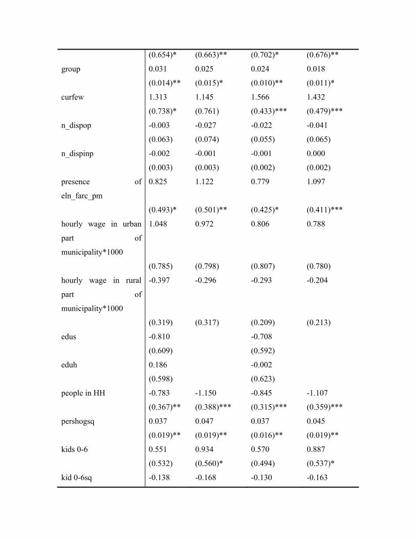
(0.654)* (0.663)** (0.702)* (0.676)**

group 0.031 0.025 0.024 0.018

(0.014)** (0.015)* (0.010)** (0.011)*

curfew 1.313 1.145 1.566 1.432

(0.738)* (0.761) (0.433)*** (0.479)***

n_dispop -0.003 -0.027 -0.022 -0.041

(0.063) (0.074) (0.055) (0.065)

n_dispinp -0.002 -0.001 -0.001 0.000

(0.003) (0.003) (0.002) (0.002)

presence of

eln_farc_pm

0.825 1.122 0.779 1.097

(0.493)* (0.501)** (0.425)* (0.411)***

hourly wage in urban

part of

municipality*1000

1.048 0.972 0.806 0.788

(0.785) (0.798) (0.807) (0.780)

hourly wage in rural

part of

municipality*1000

-0.397 -0.296 -0.293 -0.204

(0.319) (0.317) (0.209) (0.213)

edus -0.810 -0.708

(0.609) (0.592)

eduh 0.186 -0.002

(0.598) (0.623)

people in HH -0.783 -1.150 -0.845 -1.107

(0.367)** (0.388)*** (0.315)*** (0.359)***

pershogsq 0.037 0.047 0.037 0.045

(0.019)** (0.019)** (0.016)** (0.019)**

kids 0-6 0.551 0.934 0.570 0.887

(0.532) (0.560)* (0.494) (0.537)*

kid 0-6sq -0.138 -0.168 -0.130 -0.163

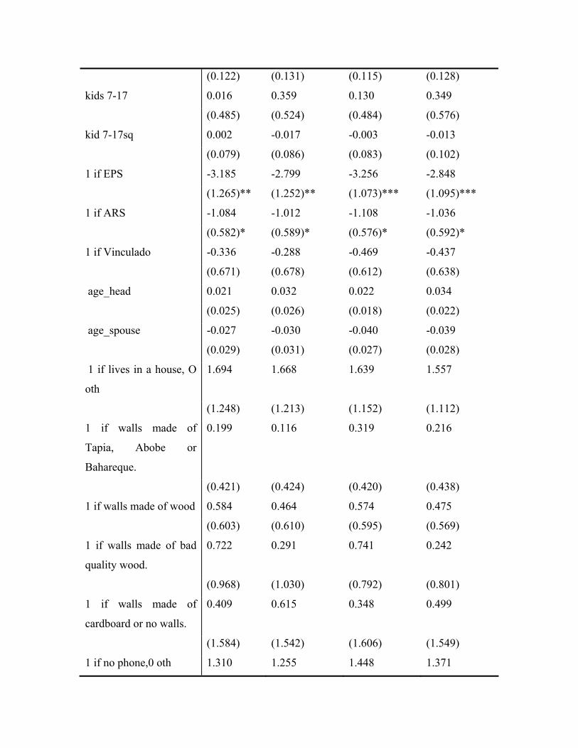
(0.122) (0.131) (0.115) (0.128)

kids 7-17 0.016 0.359 0.130 0.349

(0.485) (0.524) (0.484) (0.576)

kid 7-17sq 0.002 -0.017 -0.003 -0.013

(0.079) (0.086) (0.083) (0.102)

1 if EPS -3.185 -2.799 -3.256 -2.848

(1.265)** (1.252)** (1.073)*** (1.095)***

1 if ARS -1.084 -1.012 -1.108 -1.036

(0.582)* (0.589)* (0.576)* (0.592)*

1 if Vinculado -0.336 -0.288 -0.469 -0.437

(0.671) (0.678) (0.612) (0.638)

age_head 0.021 0.032 0.022 0.034

(0.025) (0.026) (0.018) (0.022)

age_spouse -0.027 -0.030 -0.040 -0.039

(0.029) (0.031) (0.027) (0.028)

1 if lives in a house, O

oth

1.694 1.668 1.639 1.557

(1.248) (1.213) (1.152) (1.112)

1 if walls made of

Tapia, Abobe or

Bahareque.

0.199 0.116 0.319 0.216

(0.421) (0.424) (0.420) (0.438)

1 if walls made of wood 0.584 0.464 0.574 0.475

(0.603) (0.610) (0.595) (0.569)

1 if walls made of bad

quality wood.

0.722 0.291 0.741 0.242

(0.968) (1.030) (0.792) (0.801)

1 if walls made of

cardboard or no walls.

0.409 0.615 0.348 0.499

(1.584) (1.542) (1.606) (1.549)

1 if no phone,0 oth 1.310 1.255 1.448 1.371

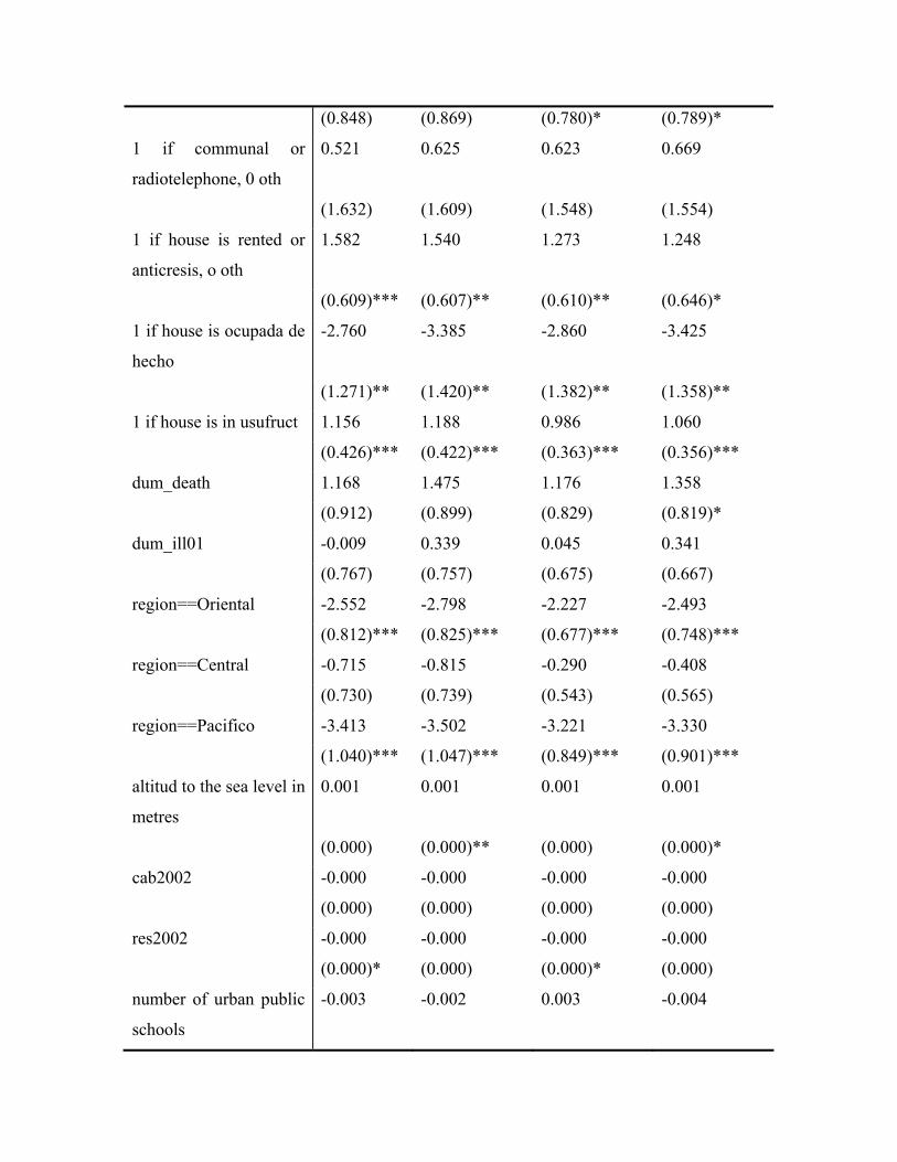
(0.848) (0.869) (0.780)* (0.789)*

1 if communal or

radiotelephone, 0 oth

0.521 0.625 0.623 0.669

(1.632) (1.609) (1.548) (1.554)

1 if house is rented or

anticresis, o oth

1.582 1.540 1.273 1.248

(0.609)*** (0.607)** (0.610)** (0.646)*

1 if house is ocupada de

hecho

-2.760 -3.385 -2.860 -3.425

(1.271)** (1.420)** (1.382)** (1.358)**

1 if house is in usufruct 1.156 1.188 0.986 1.060

(0.426)*** (0.422)*** (0.363)*** (0.356)***

dum_death 1.168 1.475 1.176 1.358

(0.912) (0.899) (0.829) (0.819)*

dum_ill01 -0.009 0.339 0.045 0.341

(0.767) (0.757) (0.675) (0.667)

region==Oriental -2.552 -2.798 -2.227 -2.493

(0.812)*** (0.825)*** (0.677)*** (0.748)***

region==Central -0.715 -0.815 -0.290 -0.408

(0.730) (0.739) (0.543) (0.565)

region==Pacifico -3.413 -3.502 -3.221 -3.330

(1.040)*** (1.047)*** (0.849)*** (0.901)***

altitud to the sea level in

metres

0.001 0.001 0.001 0.001

(0.000) (0.000)** (0.000) (0.000)*

cab2002 -0.000 -0.000 -0.000 -0.000

(0.000) (0.000) (0.000) (0.000)

res2002 -0.000 -0.000 -0.000 -0.000

(0.000)* (0.000) (0.000)* (0.000)

number of urban public

schools

-0.003 -0.002 0.003 -0.004

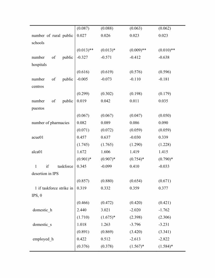
(0.087) (0.088) (0.063) (0.062)

number of rural public

schools

0.027 0.026 0.023 0.023

(0.013)** (0.013)* (0.009)** (0.010)**

number of public

hospitals

-0.327 -0.571 -0.412 -0.638

(0.616) (0.619) (0.576) (0.596)

number of public

centros

-0.005 -0.073 -0.110 -0.181

(0.299) (0.302) (0.198) (0.179)

number of public

puestos

0.019 0.042 0.011 0.035

(0.067) (0.067) (0.047) (0.050)

number of pharmacies 0.082 0.089 0.086 0.090

(0.071) (0.072) (0.059) (0.059)

acue01 0.457 0.637 -0.030 0.339

(1.745) (1.765) (1.290) (1.228)

alca01 1.672 1.606 1.419 1.415

(0.901)* (0.907)* (0.754)* (0.790)*

1 if taskforce

desertion in IPS

0.345 -0.099 0.410 -0.033

(0.857) (0.880) (0.654) (0.671)

1 if taskforce strike in

IPS, 0

0.319 0.332 0.359 0.377

(0.466) (0.472) (0.420) (0.421)

domestic_h 2.440 3.021 -2.020 -1.762

(1.710) (1.675)* (2.398) (2.306)

domestic_s 1.018 1.263 -3.796 -3.231

(0.891) (0.869) (3.420) (3.341)

employed_h 0.422 0.512 -2.613 -2.822

(0.376) (0.378) (1.567)* (1.584)*

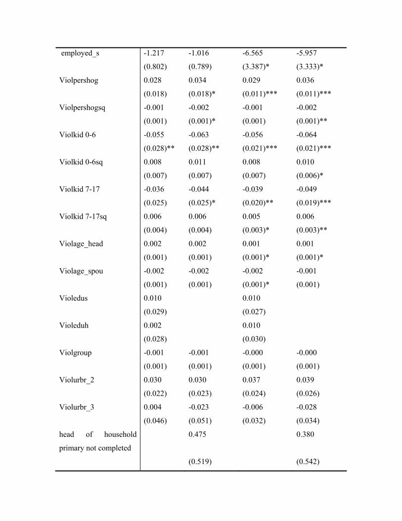
employed_s -1.217 -1.016 -6.565 -5.957

(0.802) (0.789) (3.387)* (3.333)*

Violpershog 0.028 0.034 0.029 0.036

(0.018) (0.018)* (0.011)*** (0.011)***

Violpershogsq -0.001 -0.002 -0.001 -0.002

(0.001) (0.001)* (0.001) (0.001)**

Violkid 0-6 -0.055 -0.063 -0.056 -0.064

(0.028)** (0.028)** (0.021)*** (0.021)***

Violkid 0-6sq 0.008 0.011 0.008 0.010

(0.007) (0.007) (0.007) (0.006)*

Violkid 7-17 -0.036 -0.044 -0.039 -0.049

(0.025) (0.025)* (0.020)** (0.019)***

Violkid 7-17sq 0.006 0.006 0.005 0.006

(0.004) (0.004) (0.003)* (0.003)**

Violage_head 0.002 0.002 0.001 0.001

(0.001) (0.001) (0.001)* (0.001)*

Violage_spou -0.002 -0.002 -0.002 -0.001

(0.001) (0.001) (0.001)* (0.001)

Violedus 0.010 0.010

(0.029) (0.027)

Violeduh 0.002 0.010

(0.028) (0.030)

Violgroup -0.001 -0.001 -0.000 -0.000

(0.001) (0.001) (0.001) (0.001)

Violurbr_2 0.030 0.030 0.037 0.039

(0.022) (0.023) (0.024) (0.026)

Violurbr_3 0.004 -0.023 -0.006 -0.028

(0.046) (0.051) (0.032) (0.034)

head of household

primary not completed

0.475 0.380

(0.519) (0.542)

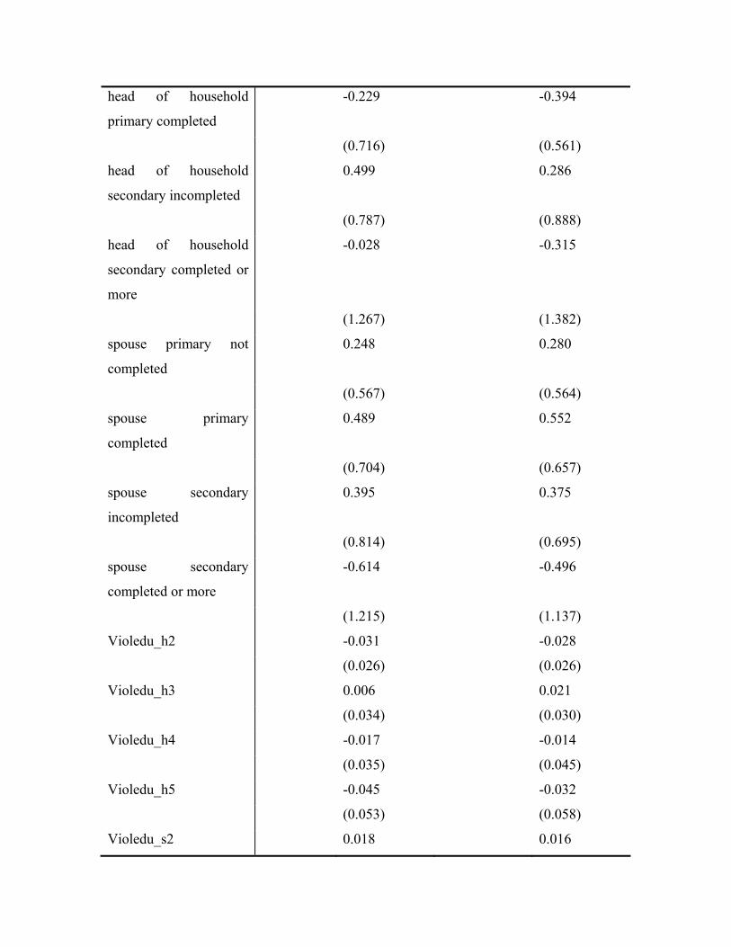
head of household

primary completed

-0.229 -0.394

(0.716) (0.561)

head of household

secondary incompleted

0.499 0.286

(0.787) (0.888)

head of household

secondary completed or

more

-0.028 -0.315

(1.267) (1.382)

spouse primary not

completed

0.248 0.280

(0.567) (0.564)

spouse primary

completed

0.489 0.552

(0.704) (0.657)

spouse secondary

incompleted

0.395 0.375

(0.814) (0.695)

spouse secondary

completed or more

-0.614 -0.496

(1.215) (1.137)

Violedu_h2 -0.031 -0.028

(0.026) (0.026)

Violedu_h3 0.006 0.021

(0.034) (0.030)

Violedu_h4 -0.017 -0.014

(0.035) (0.045)

Violedu_h5 -0.045 -0.032

(0.053) (0.058)

Violedu_s2 0.018 0.016

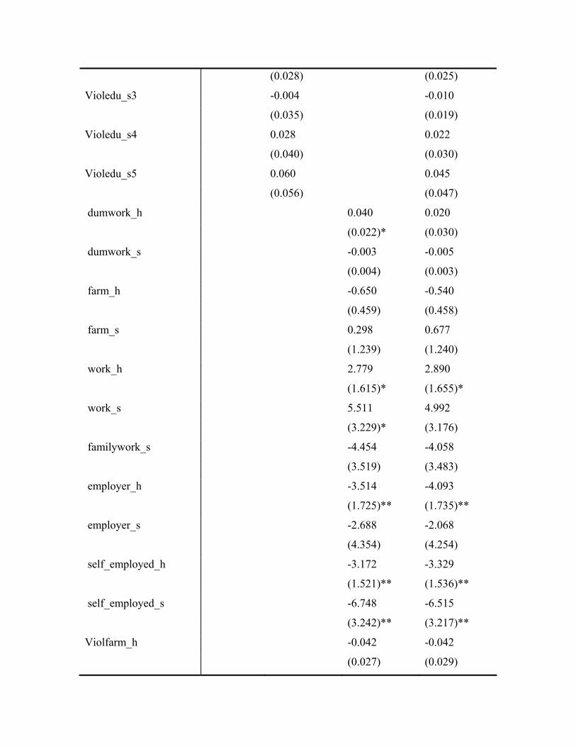
(0.028) (0.025)

Violedu_s3 -0.004 -0.010

(0.035) (0.019)

Violedu_s4 0.028 0.022

(0.040) (0.030)

Violedu_s5 0.060 0.045

(0.056) (0.047)

dumwork_h 0.040 0.020

(0.022)* (0.030)

dumwork_s -0.003 -0.005

(0.004) (0.003)

farm_h -0.650 -0.540

(0.459) (0.458)

farm_s 0.298 0.677

(1.239) (1.240)

work_h 2.779 2.890

(1.615)* (1.655)*

work_s 5.511 4.992

(3.229)* (3.176)

familywork_s -4.454 -4.058

(3.519) (3.483)

employer_h -3.514 -4.093

(1.725)** (1.735)**

employer_s -2.688 -2.068

(4.354) (4.254)

self_employed_h -3.172 -3.329

(1.521)** (1.536)**

self_employed_s -6.748 -6.515

(3.242)** (3.217)**

Violfarm_h -0.042 -0.042

(0.027) (0.029)

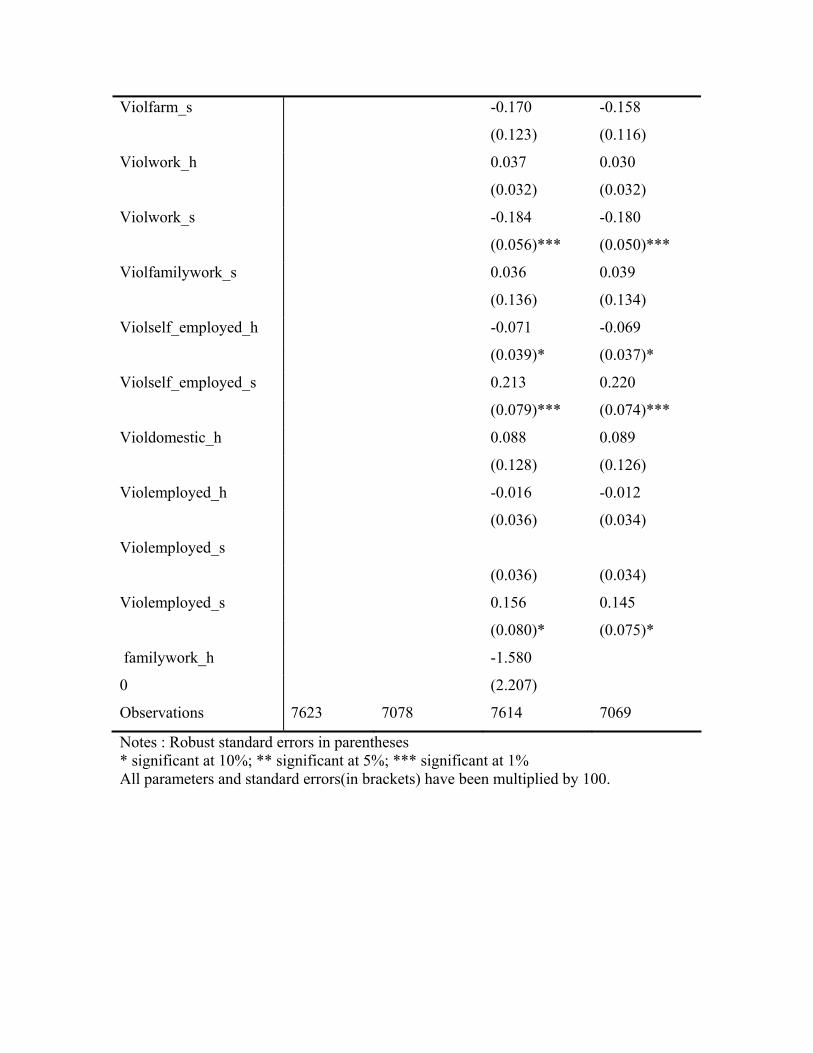
Violfarm_s -0.170 -0.158

(0.123) (0.116)

Violwork_h 0.037 0.030

(0.032) (0.032)

Violwork_s -0.184 -0.180

(0.056)*** (0.050)***

Violfamilywork_s 0.036 0.039

(0.136) (0.134)

Violself_employed_h -0.071 -0.069

(0.039)* (0.037)*

Violself_employed_s 0.213 0.220

(0.079)*** (0.074)***

Violdomestic_h 0.088 0.089

(0.128) (0.126)

Violemployed_h -0.016 -0.012

(0.036) (0.034)

Violemployed_s

(0.036) (0.034)

Violemployed_s 0.156 0.145

(0.080)* (0.075)*

familywork_h -1.580

0 (2.207)

Observations 7623 7078 7614 7069

Notes : Robust standard errors in parentheses * significant at 10%; ** significant at 5%; *** significant at 1% All parameters and standard errors(in brackets) have been multiplied by 100.

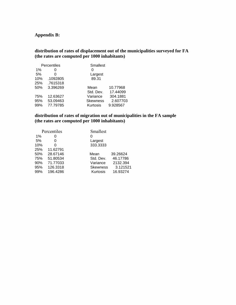
Appendix B:

distribution of rates of displacement out of the municipalities surveyed for FA (the rates are computed per 1000 inhabitants) Percentiles Smallest 1% 0 0 5% 0 Largest 10% .1092805 89.31 25% .7615318 50% 3.396269 Mean 10.77968 Std. Dev. 17.44099 75% 12.63627 Variance 304.1881 95% 53.09463 Skewness 2.607703 99% 77.79785 Kurtosis 9.928567 distribution of rates of migration out of municipalities in the FA sample (the rates are computed per 1000 inhabitants) Percentiles Smallest 1% 0 0 5% 0 Largest 10% 0 333.3333 25% 11.62791 50% 28.67146 Mean 39.26624 75% 51.80534 Std. Dev. 46.17786 90% 71.77033 Variance 2132.394 95% 126.3318 Skewness 3.121521 99% 196.4286 Kurtosis 16.93274

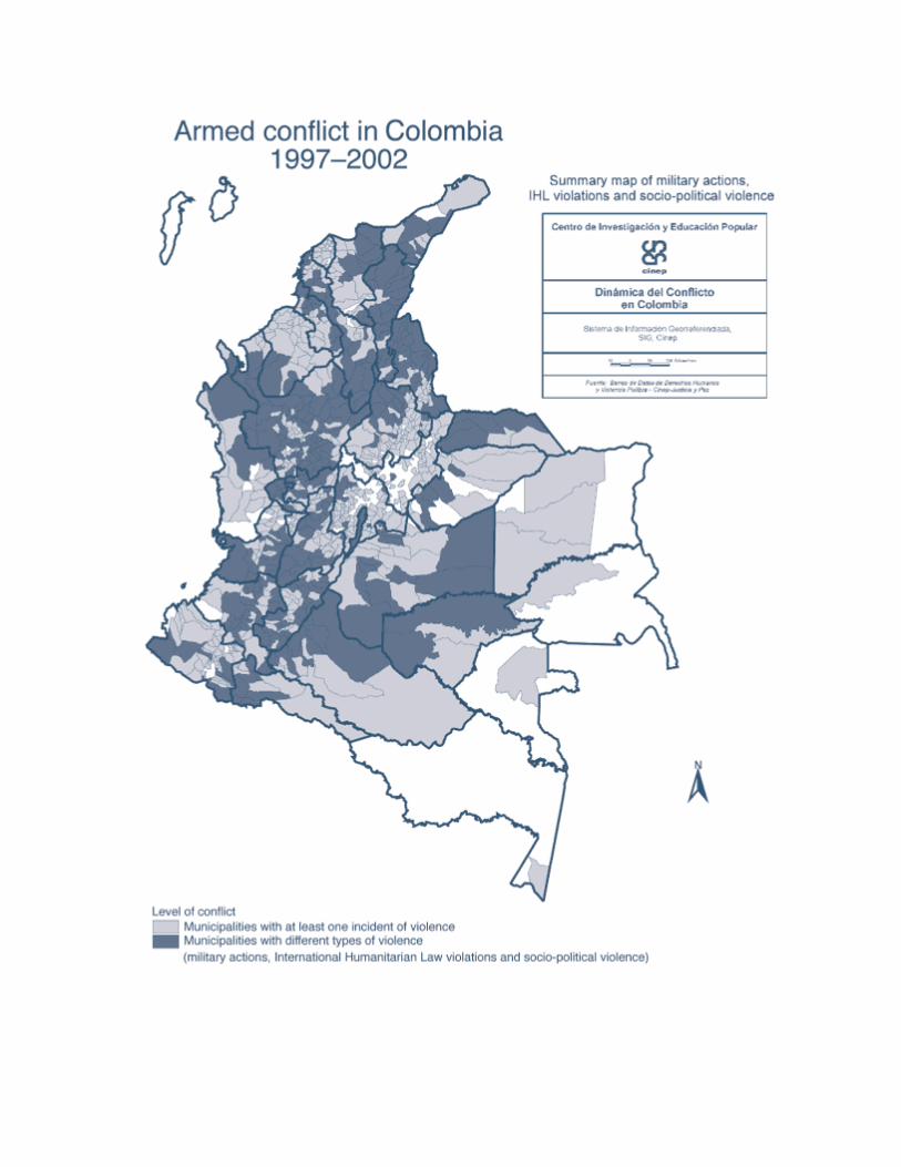
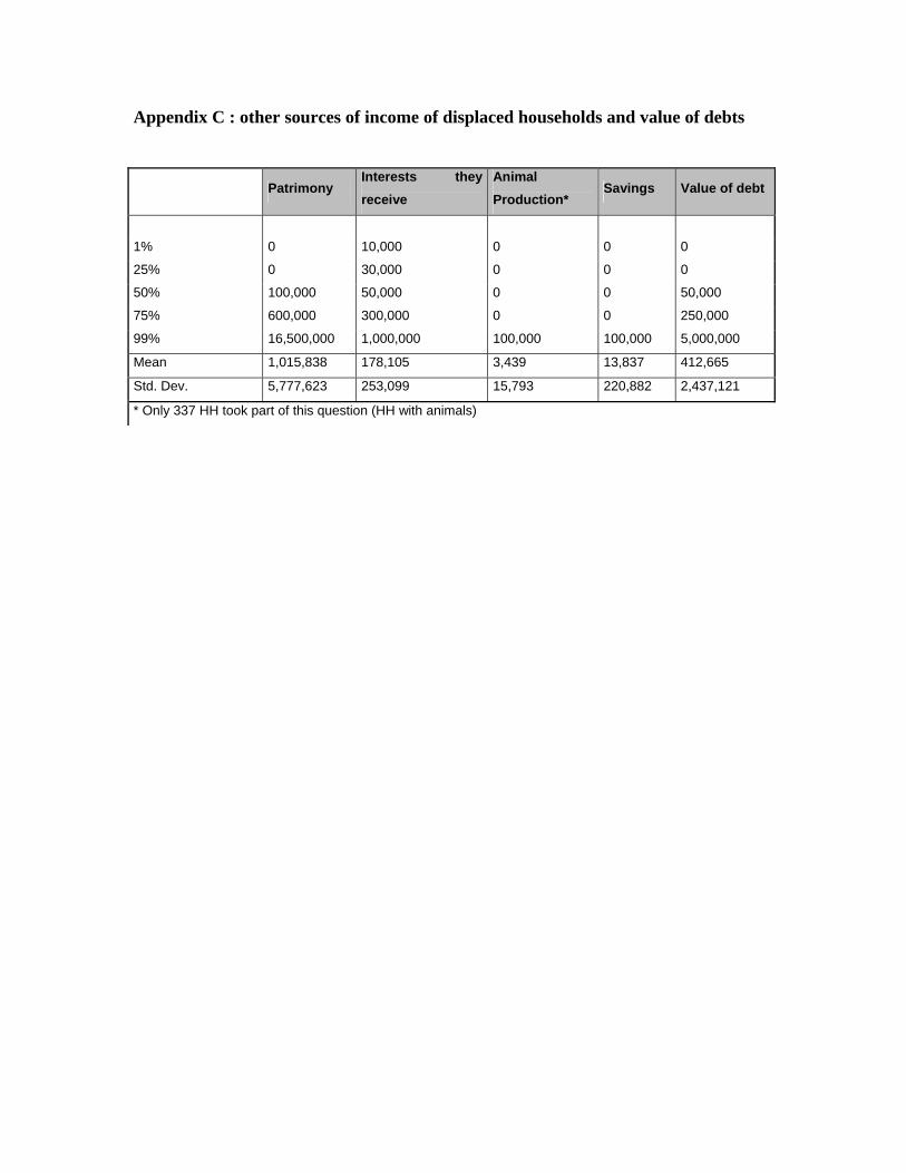
Appendix C : other sources of income of displaced households and value of debts

Patrimony

Interests they receive

Animal Production*

Savings Value of debt

1% 0 10,000 0 0 0

25% 0 30,000 0 0 0

50% 100,000 50,000 0 0 50,000

75% 600,000 300,000 0 0 250,000

99% 16,500,000 1,000,000 100,000 100,000 5,000,000

Mean 1,015,838 178,105 3,439 13,837 412,665

Std. Dev. 5,777,623 253,099 15,793 220,882 2,437,121

* Only 337 HH took part of this question (HH with animals)

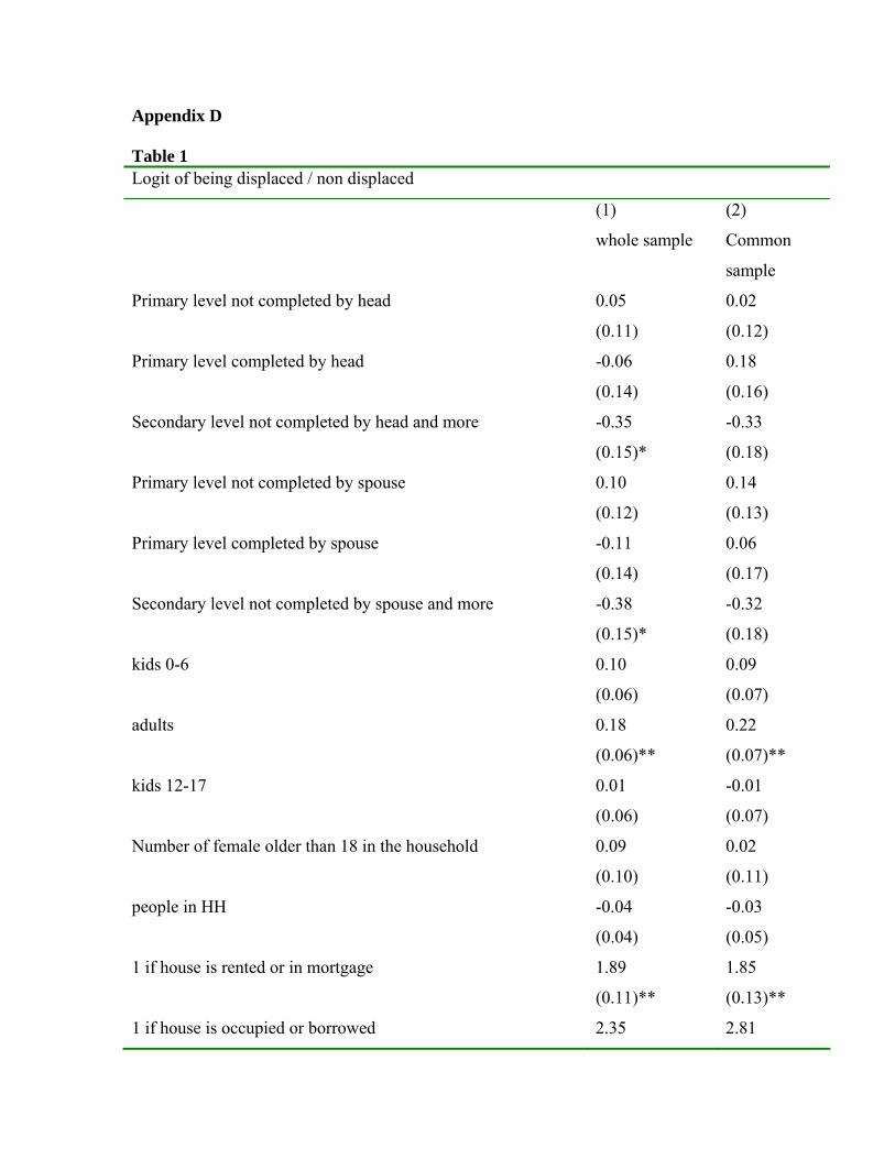
Appendix D Table 1 Logit of being displaced / non displaced

(1) (2)

whole sample Common

sample

Primary level not completed by head 0.05 0.02

(0.11) (0.12)

Primary level completed by head -0.06 0.18

(0.14) (0.16)

Secondary level not completed by head and more -0.35 -0.33

(0.15)* (0.18)

Primary level not completed by spouse 0.10 0.14

(0.12) (0.13)

Primary level completed by spouse -0.11 0.06

(0.14) (0.17)

Secondary level not completed by spouse and more -0.38 -0.32

(0.15)* (0.18)

kids 0-6 0.10 0.09

(0.06) (0.07)

adults 0.18 0.22

(0.06)** (0.07)**

kids 12-17 0.01 -0.01

(0.06) (0.07)

Number of female older than 18 in the household 0.09 0.02

(0.10) (0.11)

people in HH -0.04 -0.03

(0.04) (0.05)

1 if house is rented or in mortgage 1.89 1.85

(0.11)** (0.13)**

1 if house is occupied or borrowed 2.35 2.81

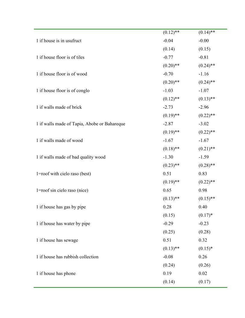
(0.12)** (0.14)**

1 if house is in usufruct -0.04 -0.00

(0.14) (0.15)

1 if house floor is of tiles -0.77 -0.81

(0.20)** (0.24)**

1 if house floor is of wood -0.70 -1.16

(0.20)** (0.24)**

1 if house floor is of conglo -1.03 -1.07

(0.12)** (0.13)**

1 if walls made of brick -2.73 -2.96

(0.19)** (0.22)**

1 if walls made of Tapia, Abobe or Bahareque -2.87 -3.02

(0.19)** (0.22)**

1 if walls made of wood -1.67 -1.67

(0.18)** (0.21)**

1 if walls made of bad quality wood -1.30 -1.59

(0.23)** (0.28)**

1=roof with cielo raso (best) 0.51 0.83

(0.19)** (0.22)**

1=roof sin cielo raso (nice) 0.65 0.98

(0.13)** (0.15)**

1 if house has gas by pipe 0.28 0.40

(0.15) (0.17)*

1 if house has water by pipe -0.29 -0.23

(0.25) (0.28)

1 if house has sewage 0.51 0.32

(0.13)** (0.15)*

1 if house has rubbish collection -0.08 0.26

(0.24) (0.26)

1 if house has phone 0.19 0.02

(0.14) (0.17)

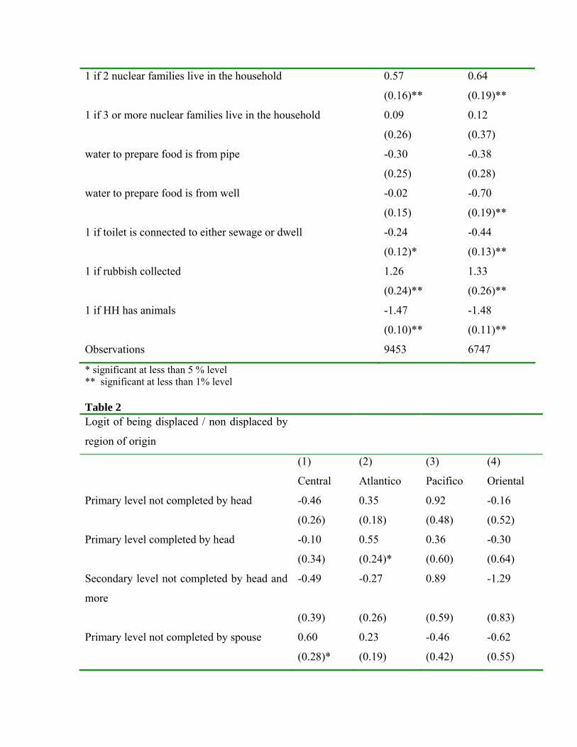
1 if 2 nuclear families live in the household 0.57 0.64

(0.16)** (0.19)**

1 if 3 or more nuclear families live in the household 0.09 0.12

(0.26) (0.37)

water to prepare food is from pipe -0.30 -0.38

(0.25) (0.28)

water to prepare food is from well -0.02 -0.70

(0.15) (0.19)**

1 if toilet is connected to either sewage or dwell -0.24 -0.44

(0.12)* (0.13)**

1 if rubbish collected 1.26 1.33

(0.24)** (0.26)**

1 if HH has animals -1.47 -1.48

(0.10)** (0.11)**

Observations 9453 6747

* significant at less than 5 % level ** significant at less than 1% level Table 2 Logit of being displaced / non displaced by

region of origin

(1) (2) (3) (4)

Central Atlantico Pacifico Oriental

Primary level not completed by head -0.46 0.35 0.92 -0.16

(0.26) (0.18) (0.48) (0.52)

Primary level completed by head -0.10 0.55 0.36 -0.30

(0.34) (0.24)* (0.60) (0.64)

Secondary level not completed by head and

more

-0.49 -0.27 0.89 -1.29

(0.39) (0.26) (0.59) (0.83)

Primary level not completed by spouse 0.60 0.23 -0.46 -0.62

(0.28)* (0.19) (0.42) (0.55)

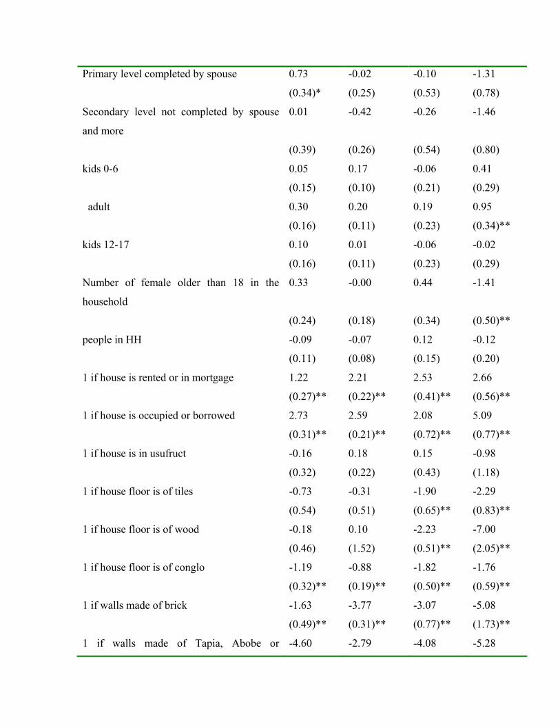
Primary level completed by spouse 0.73 -0.02 -0.10 -1.31

(0.34)* (0.25) (0.53) (0.78)

Secondary level not completed by spouse

and more

0.01 -0.42 -0.26 -1.46

(0.39) (0.26) (0.54) (0.80)

kids 0-6 0.05 0.17 -0.06 0.41

(0.15) (0.10) (0.21) (0.29)

adult 0.30 0.20 0.19 0.95

(0.16) (0.11) (0.23) (0.34)**

kids 12-17 0.10 0.01 -0.06 -0.02

(0.16) (0.11) (0.23) (0.29)

Number of female older than 18 in the

household

0.33 -0.00 0.44 -1.41

(0.24) (0.18) (0.34) (0.50)**

people in HH -0.09 -0.07 0.12 -0.12

(0.11) (0.08) (0.15) (0.20)

1 if house is rented or in mortgage 1.22 2.21 2.53 2.66

(0.27)** (0.22)** (0.41)** (0.56)**

1 if house is occupied or borrowed 2.73 2.59 2.08 5.09

(0.31)** (0.21)** (0.72)** (0.77)**

1 if house is in usufruct -0.16 0.18 0.15 -0.98

(0.32) (0.22) (0.43) (1.18)

1 if house floor is of tiles -0.73 -0.31 -1.90 -2.29

(0.54) (0.51) (0.65)** (0.83)**

1 if house floor is of wood -0.18 0.10 -2.23 -7.00

(0.46) (1.52) (0.51)** (2.05)**

1 if house floor is of conglo -1.19 -0.88 -1.82 -1.76

(0.32)** (0.19)** (0.50)** (0.59)**

1 if walls made of brick -1.63 -3.77 -3.07 -5.08

(0.49)** (0.31)** (0.77)** (1.73)**

1 if walls made of Tapia, Abobe or -4.60 -2.79 -4.08 -5.28

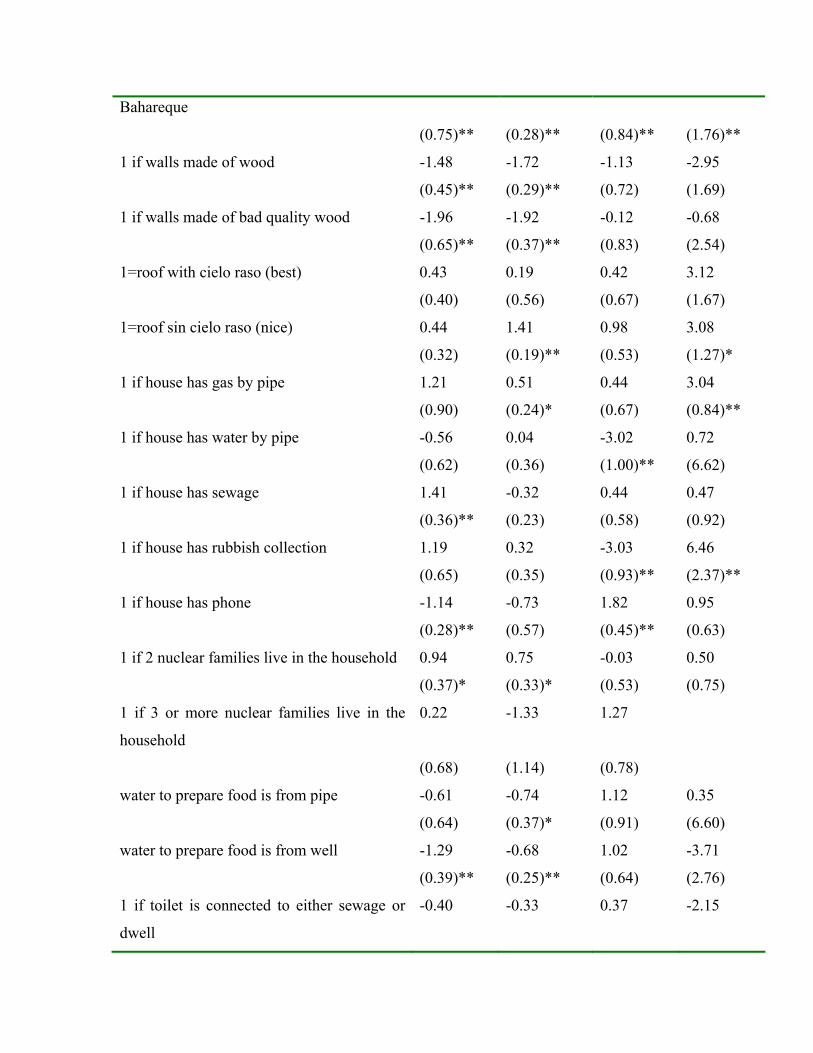
Bahareque

(0.75)** (0.28)** (0.84)** (1.76)**

1 if walls made of wood -1.48 -1.72 -1.13 -2.95

(0.45)** (0.29)** (0.72) (1.69)

1 if walls made of bad quality wood -1.96 -1.92 -0.12 -0.68

(0.65)** (0.37)** (0.83) (2.54)

1=roof with cielo raso (best) 0.43 0.19 0.42 3.12

(0.40) (0.56) (0.67) (1.67)

1=roof sin cielo raso (nice) 0.44 1.41 0.98 3.08

(0.32) (0.19)** (0.53) (1.27)*

1 if house has gas by pipe 1.21 0.51 0.44 3.04

(0.90) (0.24)* (0.67) (0.84)**

1 if house has water by pipe -0.56 0.04 -3.02 0.72

(0.62) (0.36) (1.00)** (6.62)

1 if house has sewage 1.41 -0.32 0.44 0.47

(0.36)** (0.23) (0.58) (0.92)

1 if house has rubbish collection 1.19 0.32 -3.03 6.46

(0.65) (0.35) (0.93)** (2.37)**

1 if house has phone -1.14 -0.73 1.82 0.95

(0.28)** (0.57) (0.45)** (0.63)

1 if 2 nuclear families live in the household 0.94 0.75 -0.03 0.50

(0.37)* (0.33)* (0.53) (0.75)

1 if 3 or more nuclear families live in the

household

0.22 -1.33 1.27

(0.68) (1.14) (0.78)

water to prepare food is from pipe -0.61 -0.74 1.12 0.35

(0.64) (0.37)* (0.91) (6.60)

water to prepare food is from well -1.29 -0.68 1.02 -3.71

(0.39)** (0.25)** (0.64) (2.76)

1 if toilet is connected to either sewage or

dwell

-0.40 -0.33 0.37 -2.15

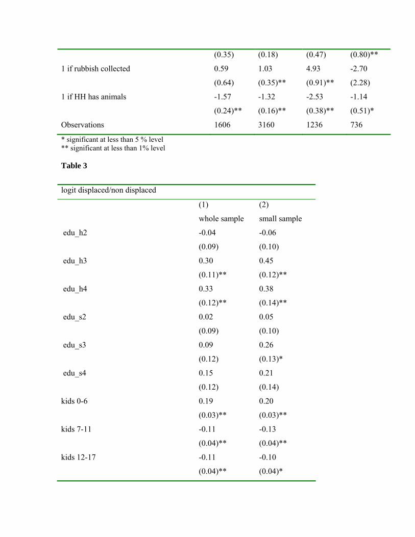
(0.35) (0.18) (0.47) (0.80)**

1 if rubbish collected 0.59 1.03 4.93 -2.70

(0.64) (0.35)** (0.91)** (2.28)

1 if HH has animals -1.57 -1.32 -2.53 -1.14

(0.24)** (0.16)** (0.38)** (0.51)*

Observations 1606 3160 1236 736

* significant at less than 5 % level ** significant at less than 1% level Table 3

logit displaced/non displaced

(1) (2)

whole sample small sample

edu_h2 -0.04 -0.06

(0.09) (0.10)

edu_h3 0.30 0.45

(0.11)** (0.12)**

edu_h4 0.33 0.38

(0.12)** (0.14)**

edu_s2 0.02 0.05

(0.09) (0.10)

edu_s3 0.09 0.26

(0.12) (0.13)*

edu_s4 0.15 0.21

(0.12) (0.14)

kids 0-6 0.19 0.20

(0.03)** (0.03)**

kids 7-11 -0.11 -0.13

(0.04)** (0.04)**

kids 12-17 -0.11 -0.10

(0.04)** (0.04)*

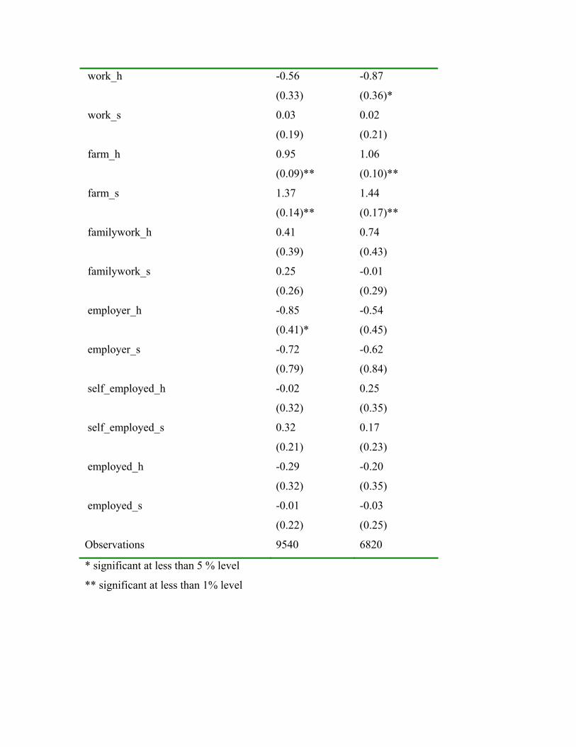
work_h -0.56 -0.87

(0.33) (0.36)*

work_s 0.03 0.02

(0.19) (0.21)

farm_h 0.95 1.06

(0.09)** (0.10)**

farm_s 1.37 1.44

(0.14)** (0.17)**

familywork_h 0.41 0.74

(0.39) (0.43)

familywork_s 0.25 -0.01

(0.26) (0.29)

employer_h -0.85 -0.54

(0.41)* (0.45)

employer_s -0.72 -0.62

(0.79) (0.84)

self_employed_h -0.02 0.25

(0.32) (0.35)

self_employed_s 0.32 0.17

(0.21) (0.23)

employed_h -0.29 -0.20

(0.32) (0.35)

employed_s -0.01 -0.03

(0.22) (0.25)

Observations 9540 6820

* significant at less than 5 % level

** significant at less than 1% level

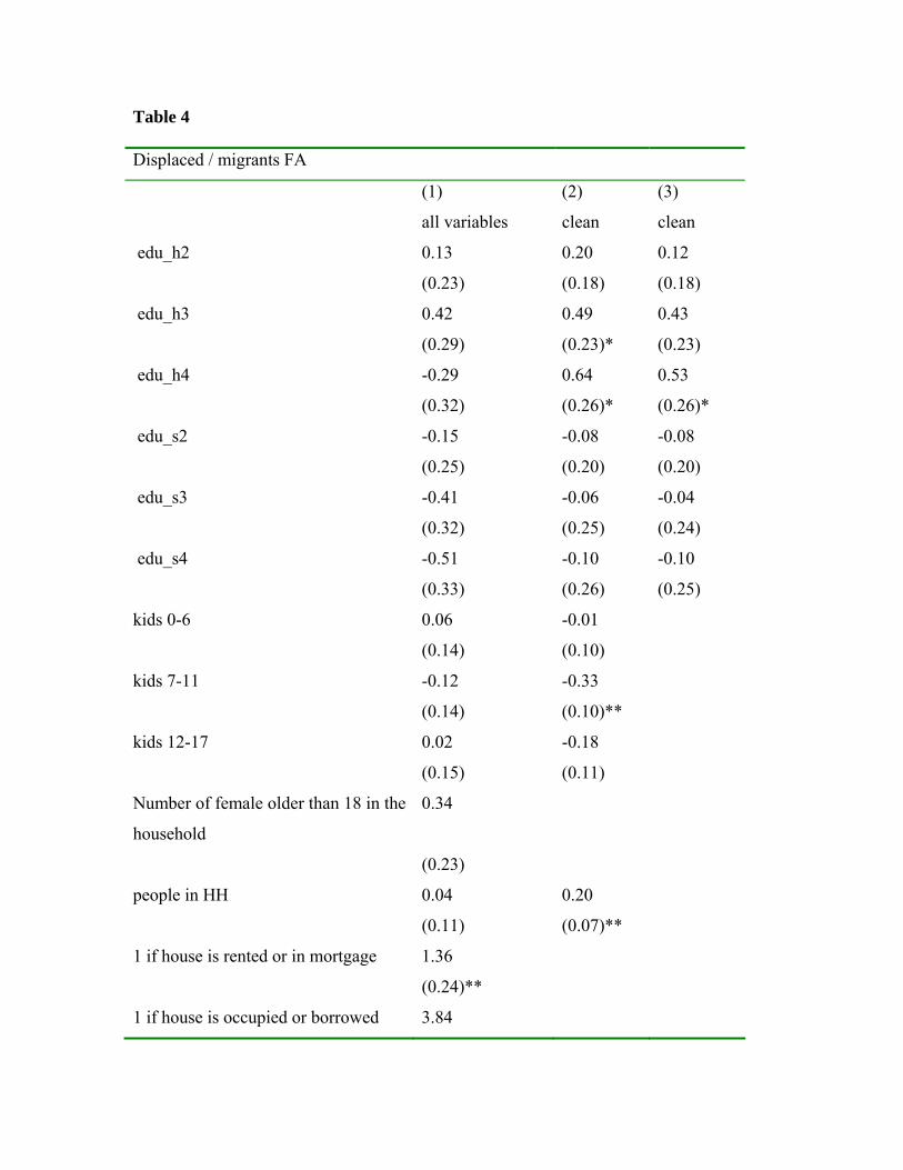
Table 4 Displaced / migrants FA

(1) (2) (3)

all variables clean clean

edu_h2 0.13 0.20 0.12

(0.23) (0.18) (0.18)

edu_h3 0.42 0.49 0.43

(0.29) (0.23)* (0.23)

edu_h4 -0.29 0.64 0.53

(0.32) (0.26)* (0.26)*

edu_s2 -0.15 -0.08 -0.08

(0.25) (0.20) (0.20)

edu_s3 -0.41 -0.06 -0.04

(0.32) (0.25) (0.24)

edu_s4 -0.51 -0.10 -0.10

(0.33) (0.26) (0.25)

kids 0-6 0.06 -0.01

(0.14) (0.10)

kids 7-11 -0.12 -0.33

(0.14) (0.10)**

kids 12-17 0.02 -0.18

(0.15) (0.11)

Number of female older than 18 in the

household

0.34

(0.23)

people in HH 0.04 0.20

(0.11) (0.07)**

1 if house is rented or in mortgage 1.36

(0.24)**

1 if house is occupied or borrowed 3.84

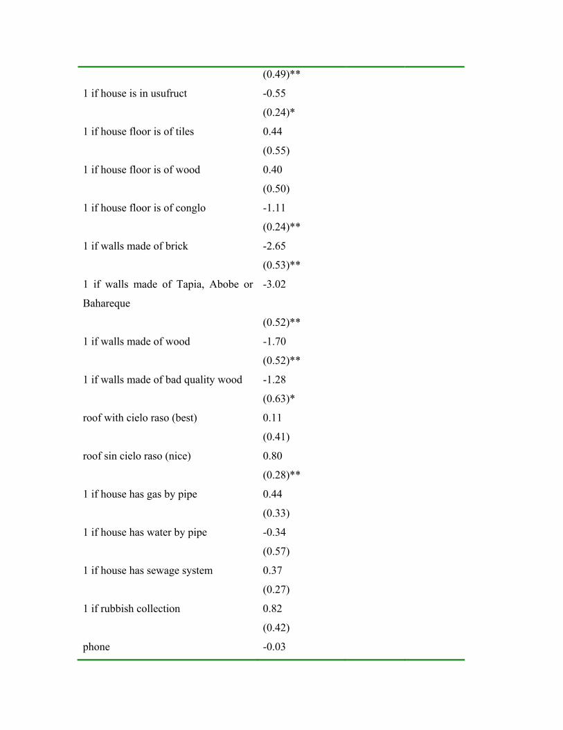
(0.49)**

1 if house is in usufruct -0.55

(0.24)*

1 if house floor is of tiles 0.44

(0.55)

1 if house floor is of wood 0.40

(0.50)

1 if house floor is of conglo -1.11

(0.24)**

1 if walls made of brick -2.65

(0.53)**

1 if walls made of Tapia, Abobe or

Bahareque

-3.02

(0.52)**

1 if walls made of wood -1.70

(0.52)**

1 if walls made of bad quality wood -1.28

(0.63)*

roof with cielo raso (best) 0.11

(0.41)

roof sin cielo raso (nice) 0.80

(0.28)**

1 if house has gas by pipe 0.44

(0.33)

1 if house has water by pipe -0.34

(0.57)

1 if house has sewage system 0.37

(0.27)

1 if rubbish collection 0.82

(0.42)

phone -0.03

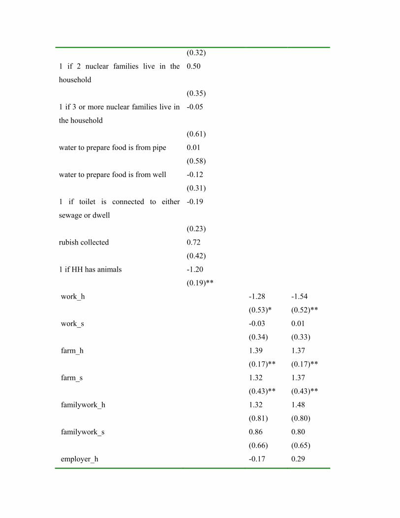
(0.32)

1 if 2 nuclear families live in the

household

0.50

(0.35)

1 if 3 or more nuclear families live in

the household

-0.05

(0.61)

water to prepare food is from pipe 0.01

(0.58)

water to prepare food is from well -0.12

(0.31)

1 if toilet is connected to either

sewage or dwell

-0.19

(0.23)

rubish collected 0.72

(0.42)

1 if HH has animals -1.20

(0.19)**

work_h -1.28 -1.54

(0.53)* (0.52)**

work_s -0.03 0.01

(0.34) (0.33)

farm_h 1.39 1.37

(0.17)** (0.17)**

farm_s 1.32 1.37

(0.43)** (0.43)**

familywork_h 1.32 1.48

(0.81) (0.80)

familywork_s 0.86 0.80

(0.66) (0.65)

employer_h -0.17 0.29

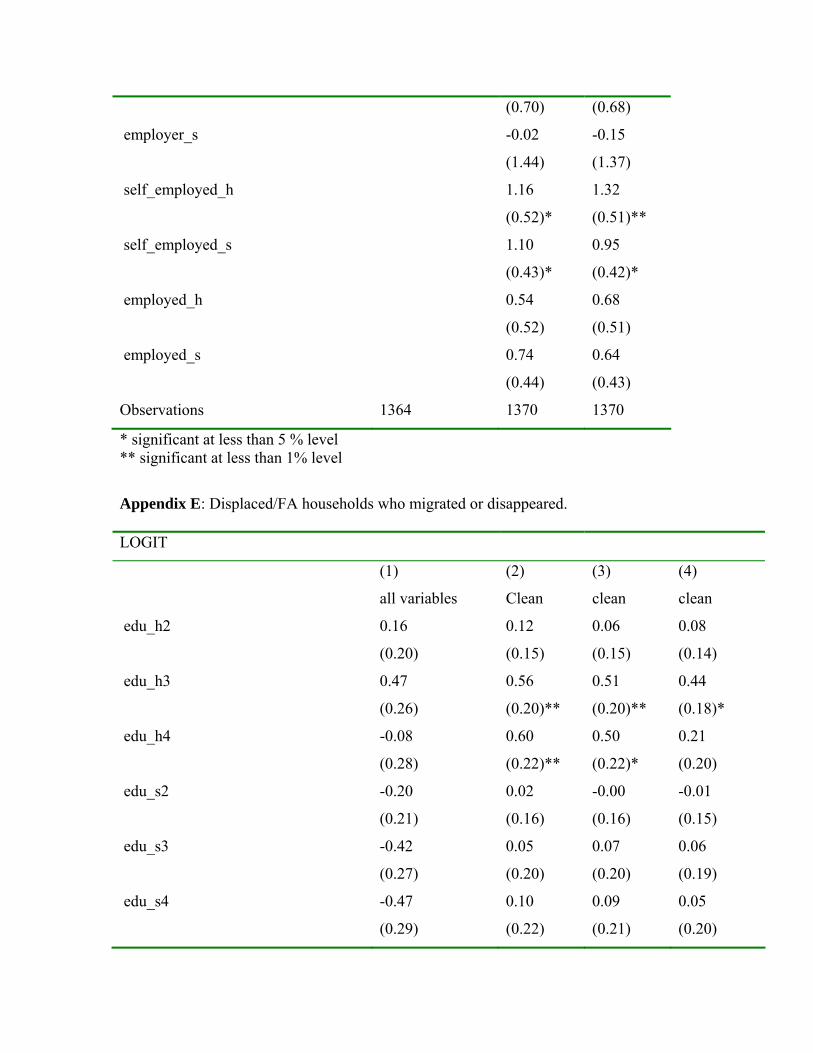
(0.70) (0.68)

employer_s -0.02 -0.15

(1.44) (1.37)

self_employed_h 1.16 1.32

(0.52)* (0.51)**

self_employed_s 1.10 0.95

(0.43)* (0.42)*

employed_h 0.54 0.68

(0.52) (0.51)

employed_s 0.74 0.64

(0.44) (0.43)

Observations 1364 1370 1370

* significant at less than 5 % level ** significant at less than 1% level

Appendix E: Displaced/FA households who migrated or disappeared. LOGIT

(1) (2) (3) (4)

all variables Clean clean clean

edu_h2 0.16 0.12 0.06 0.08

(0.20) (0.15) (0.15) (0.14)

edu_h3 0.47 0.56 0.51 0.44

(0.26) (0.20)** (0.20)** (0.18)*

edu_h4 -0.08 0.60 0.50 0.21

(0.28) (0.22)** (0.22)* (0.20)

edu_s2 -0.20 0.02 -0.00 -0.01

(0.21) (0.16) (0.16) (0.15)

edu_s3 -0.42 0.05 0.07 0.06

(0.27) (0.20) (0.20) (0.19)

edu_s4 -0.47 0.10 0.09 0.05

(0.29) (0.22) (0.21) (0.20)

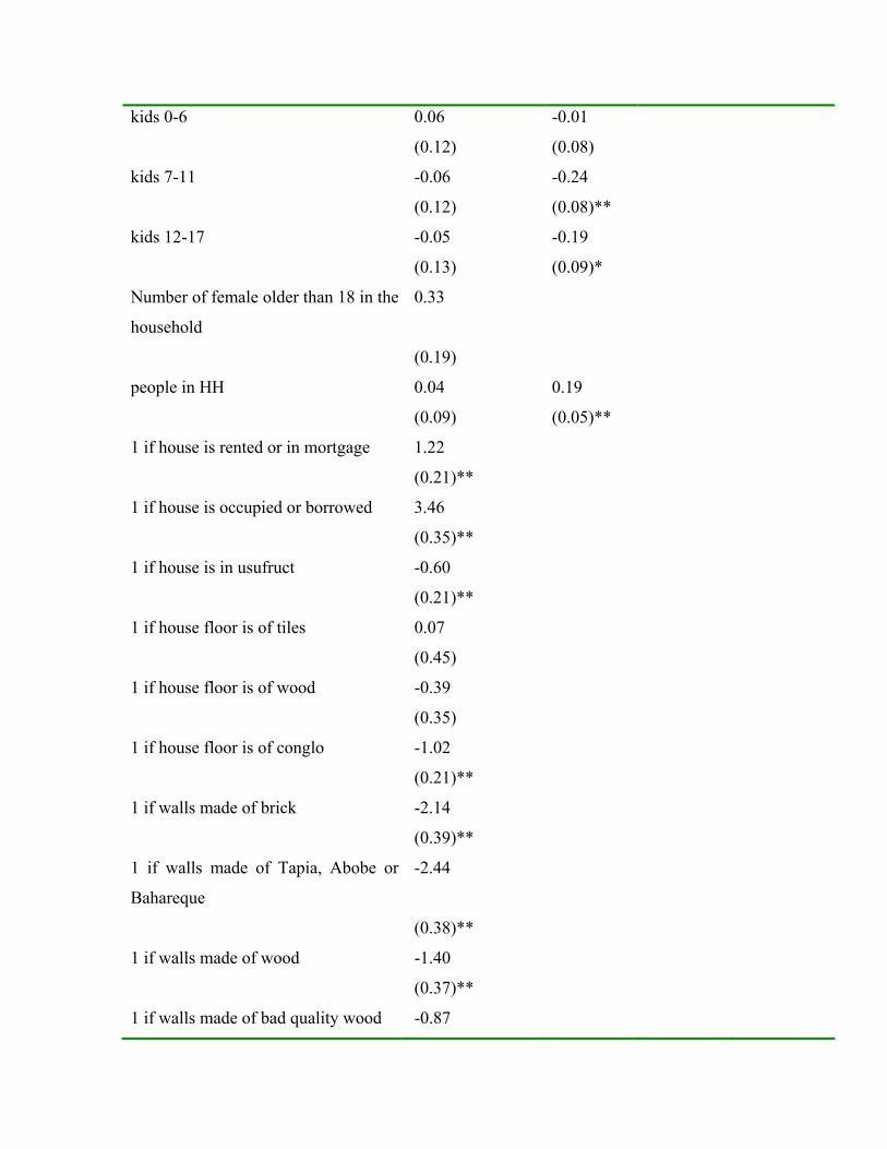
kids 0-6 0.06 -0.01

(0.12) (0.08)

kids 7-11 -0.06 -0.24

(0.12) (0.08)**

kids 12-17 -0.05 -0.19

(0.13) (0.09)*

Number of female older than 18 in the

household

0.33

(0.19)

people in HH 0.04 0.19

(0.09) (0.05)**

1 if house is rented or in mortgage 1.22

(0.21)**

1 if house is occupied or borrowed 3.46

(0.35)**

1 if house is in usufruct -0.60

(0.21)**

1 if house floor is of tiles 0.07

(0.45)

1 if house floor is of wood -0.39

(0.35)

1 if house floor is of conglo -1.02

(0.21)**

1 if walls made of brick -2.14

(0.39)**

1 if walls made of Tapia, Abobe or

Bahareque

-2.44

(0.38)**

1 if walls made of wood -1.40

(0.37)**

1 if walls made of bad quality wood -0.87

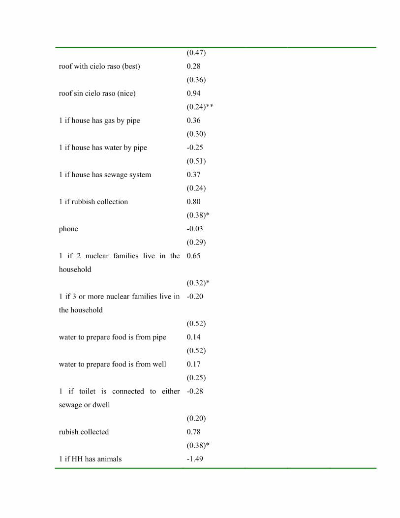
(0.47)

roof with cielo raso (best) 0.28

(0.36)

roof sin cielo raso (nice) 0.94

(0.24)**

1 if house has gas by pipe 0.36

(0.30)

1 if house has water by pipe -0.25

(0.51)

1 if house has sewage system 0.37

(0.24)

1 if rubbish collection 0.80

(0.38)*

phone -0.03

(0.29)

1 if 2 nuclear families live in the

household

0.65

(0.32)*

1 if 3 or more nuclear families live in

the household

-0.20

(0.52)

water to prepare food is from pipe 0.14

(0.52)

water to prepare food is from well 0.17

(0.25)

1 if toilet is connected to either

sewage or dwell

-0.28

(0.20)

rubish collected 0.78

(0.38)*

1 if HH has animals -1.49

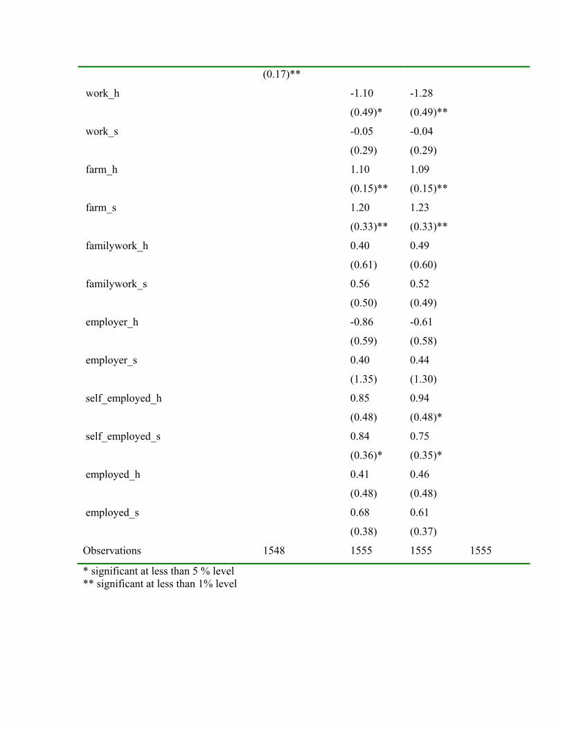
(0.17)**

work_h -1.10 -1.28

(0.49)* (0.49)**

work_s -0.05 -0.04

(0.29) (0.29)

farm_h 1.10 1.09

(0.15)** (0.15)**

farm_s 1.20 1.23

(0.33)** (0.33)**

familywork_h 0.40 0.49

(0.61) (0.60)

familywork_s 0.56 0.52

(0.50) (0.49)

employer_h -0.86 -0.61

(0.59) (0.58)

employer_s 0.40 0.44

(1.35) (1.30)

self_employed_h 0.85 0.94

(0.48) (0.48)*

self_employed_s 0.84 0.75

(0.36)* (0.35)*

employed_h 0.41 0.46

(0.48) (0.48)

employed_s 0.68 0.61

(0.38) (0.37)

Observations 1548 1555 1555 1555

* significant at less than 5 % level ** significant at less than 1% level

Appendix F : Using economic experiments to measure social capital and attitudes

towards risk within the context of the Familias en Acción evaluation survey

By Abigail Barr and Juan-Camilo Cardenas.

1. Introduction

In late 2003 the Familias en Accion (FA) evaluation team piloted a behavioural

experiment designed to generate measures of attitudes towards risk and social capital that

could be analysed in conjunction with the survey data. Here, we report the findings from

that pilot study.

In behavioural experiments human subjects are invited to play games under controlled

conditions. The games are designed to simulate decision-making environments that

people face in everyday life. The games always involve real incentives, i.e., they are

played for money, and the decisions that each subject makes within the game, combined

with the role of a die, toss of a coin, or the decisions made by others in the game

determine how much money they take away at the end. As long as the amounts of money

at stake are sufficiently high, we can expect the subjects to take their decisions seriously

and reveal their preferences and underlying motivations through the way that they play.

Behavioural experiments are most often conducted in university laboratories with

students as subjects. This affords the experimenters a great deal of control, but has led

many to question the relevance of experiments to our understanding of how people in

general behave outside of campus. Recently, a growing number of researchers have

started running behavioural experiments in the field. These experiments have involved

farmers, fishermen, urban workers, truck drivers, school children, hunter-gatherers, and

many other subject types. They have been conducted on doorsteps, in sitting rooms, in

village meeting places, under the shade of large trees, in worker common rooms, on

beaches, in truckers’ cafes, in club houses, and in school classrooms. And they have

addressed many topics including peoples’ willingness to cooperate, whether cooperation

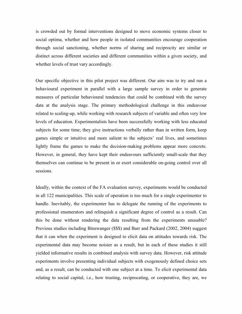
is crowded out by formal interventions designed to move economic systems closer to

social optima, whether and how people in isolated communities encourage cooperation

through social sanctioning, whether norms of sharing and reciprocity are similar or

distinct across different societies and different communities within a given society, and

whether levels of trust vary accordingly.

Our specific objective in this pilot project was different. Our aim was to try and run a

behavioural experiment in parallel with a large sample survey in order to generate

measures of particular behavioural tendencies that could be combined with the survey

data at the analysis stage. The primary methodological challenge in this endeavour

related to scaling-up, while working with research subjects of variable and often very low

levels of education. Experimentalists have been successfully working with less educated

subjects for some time; they give instructions verbally rather than in written form, keep

games simple or intuitive and more salient to the subjects’ real lives, and sometimes

lightly frame the games to make the decision-making problems appear more concrete.

However, in general, they have kept their endeavours sufficiently small-scale that they

themselves can continue to be present in or exert considerable on-going control over all

sessions.

Ideally, within the context of the FA evaluation survey, experiments would be conducted

in all 122 municipalities. This scale of operation is too much for a single experimenter to

handle. Inevitably, the experimenter has to delegate the running of the experiments to

professional enumerators and relinquish a significant degree of control as a result. Can

this be done without rendering the data resulting from the experiments unusable?

Previous studies including Binswanger ($$$) and Barr and Packard (2002, 2004) suggest

that it can when the experiment is designed to elicit data on attitudes towards risk. The

experimental data may become noisier as a result, but in each of these studies it still

yielded informative results in combined analysis with survey data. However, risk attitude

experiments involve presenting individual subjects with exogenously defined choice sets

and, as a result, can be conducted with one subject at a time. To elicit experimental data

relating to social capital, i.e., how trusting, reciprocating, or cooperative, they are, we

need to either bring subjects together so that they can really interact or cause them to

believe that they are interacting even when those with whom they are interacting are not

present. A few experimentalists have taken the latter approach, while conducting trust

experiments. Ruffle (?) working in Kibbutz in Israel, Burns (?) working with school

children in South Africa, and Cardenas (?) working with students in Bogota, each used

mobile phones to transmit information in trust games and thereby concretized playing

partners. In contrast, Fehr et al. (2003), working with adult respondents to a nationally

representative survey in Germany, took the former approach. In their study, professional

enumerators simply asserted the existence of the playing partners to the respondents

during one-on-one interviews. Fehr et al.’s data suggests that they were successful.

However, many field experimentalists believe that this approach would not work in most

contexts, especially in countries where there is less trust in formal institutions. Ruffle,

Burns, and Cardenas’ approach also appeared to work but is restricted to places where

mobile phones are effective and familiar to the subjects involved. At the piloting stage,

we did not think it appropriate to assume that mobile phones could be used effectively for

interactive experimentation in the Colombian municipalities in which the FA evaluation

is being conducted. Thus, when eliciting experimentally derived social capital measures

we restricted ourselves to only one option, to bring people together to play the interactive

games, and see if our professional enumerators could cope with the added problems of

control that would inevitably result.

During the pilot (in the last quarter of 2003) we trained 2 teams of professional

enumerators to conduct an experiment involving a single game designed to elicit

measures relating to both attitudes towards risk and social capital. Each team conducted

this experiment in six municipalities. One experimental session involving between 26 and

47 subjects was run in a central location in each municipality. This exercise yielded

experimental data relating to 12 out of the 122 municipalities covered by the FA

evaluation survey. Six of these municipalities were receiving the FA transfers and related

interventions and six were control municipalities.

Were we to return to run the experiment in all 122 municipalities, i.e., to move from pilot

to full study, we would aim to conduct the experiment in exactly the same way in all

municipalities. However, during the pilot we conducted three slightly different versions,

each version in four municipalities (two FA recipient municipalities and two control

municipalities). We did this for two reasons. First, it allowed us to look at which

treatment might work best when scaled up to all 122 municipalities. And second, it

provided us with an opportunity to compare patterns in the data with our priors about

how behaviour might vary across treatments and thereby assess whether delegating to

professional enumerators in order to scale up had compromised the quality of the

resulting data.

The results of this exercise suggest that the experiment provided potentially useful data

on both the subject’s attitudes towards risk and their social capital, or more specifically

their willingness and ability to mobilize into groups to address a collective problem.

The report is organized into six sections. Following this introduction (section 1), section

2 provides more detail on the experimental design and lists our priors relating to how

behaviour might vary across treatments. Then, in section 3 we present a graphical and

first statistical analysis of the experimental data. In section 4, we present a relational

analysis of group formation which endeavours to explain the patterns in the group

formation data with reference to the strong ties (family and friends) and weak ties

(acquaintances) between the experimental subjects that existed prior to the running of the

experiment. In section 5, we conduct a series of regression analyses on the game data,

introducing some variables derived from the SNA and some from the survey in order to

explore the effects of the FA interventions and of the ongoing violence experienced in

many municipalities in Colombia. In section 6, we draw out the lessons from this pilot

exercise and make our recommendations relating to future experimental work within the

context of the FA evaluation survey.

2. Experimental Design

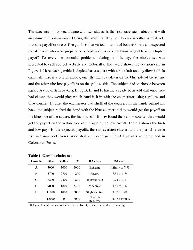
The experiment involved a game with two stages. In the first stage each subject met with

an enumerator one-on-one. During this meeting, they had to choose either a relatively

low sure payoff or one of five gambles that varied in terms of both riskiness and expected

payoff; those who were prepared to accept more risk could choose a gamble with a higher

payoff. To overcome potential problems relating to illiteracy, the choice set was

presented to each subject verbally and pictorially. They were shown the decision card in

Figure 1. Here, each gamble is depicted as a square with a blue half and a yellow half. In

each half there is a pile of money, one (the high payoff) is on the blue side of the square

and the other (the low payoff) is on the yellow side. The subject had to choose between

square A (the certain payoff), B, C, D, E, and F, having already been told that once they

had chosen they would play which-hand-is-it-in with the enumerator using a yellow and

blue counter. If, after the enumerator had shuffled the counters in his hands behind his

back, the subject picked the hand with the blue counter in they would get the payoff on

the blue side of the square, the high payoff. If they found the yellow counter they would

get the payoff on the yellow side of the square, the low payoff. Table 1 shows the high

and low payoffs, the expected payoffs, the risk aversion classes, and the partial relative

risk aversion coefficients associated with each gamble. All payoffs are presented in

Colombian Pesos.

Table 1. Gamble choice set Gamble Blue Yellow EV RA class RA coeff.

A 3000 3000 3000 Extreme Infinity to 7.51

B 5700 2700 4200 Severe 7.51 to 1.74

C 7200 2400 4800 Intermediate 1.74 to 0.81

D 9000 1800 5400 Moderate 0.81 to 0.32

E 11000 1000 6000 Slight-neutral 0.32 to 0.00

F 12000 0 6000 Neutral-negative 0 to –ve infinity

RA coefficient ranges not quite correct for D, E, and F - need recalculating

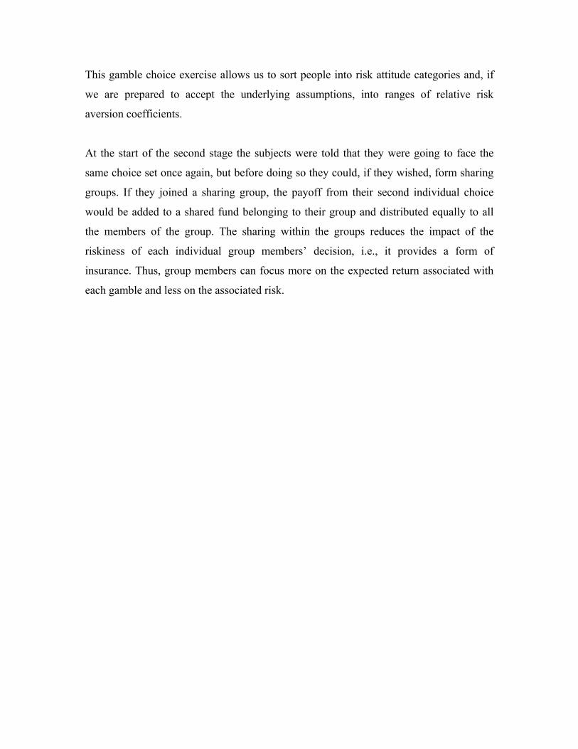
This gamble choice exercise allows us to sort people into risk attitude categories and, if

we are prepared to accept the underlying assumptions, into ranges of relative risk

aversion coefficients.

At the start of the second stage the subjects were told that they were going to face the

same choice set once again, but before doing so they could, if they wished, form sharing

groups. If they joined a sharing group, the payoff from their second individual choice

would be added to a shared fund belonging to their group and distributed equally to all

the members of the group. The sharing within the groups reduces the impact of the

riskiness of each individual group members’ decision, i.e., it provides a form of

insurance. Thus, group members can focus more on the expected return associated with

each gamble and less on the associated risk.

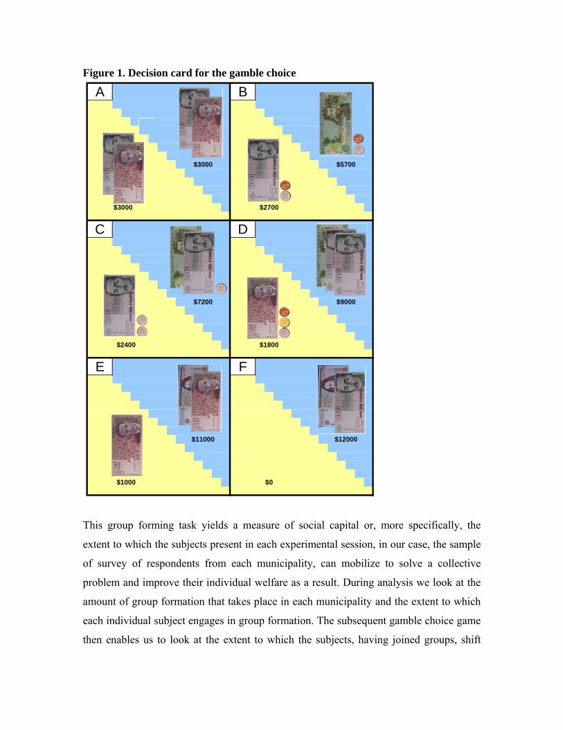
Figure 1. Decision card for the gamble choice

A B

$3000 $5700

$2700

C D

$7200 $9000

$2400 $1800

E F

$11000 $12000

$1000 $0

$3000

This group forming task yields a measure of social capital or, more specifically, the

extent to which the subjects present in each experimental session, in our case, the sample

of survey of respondents from each municipality, can mobilize to solve a collective

problem and improve their individual welfare as a result. During analysis we look at the

amount of group formation that takes place in each municipality and the extent to which

each individual subject engages in group formation. The subsequent gamble choice game

then enables us to look at the extent to which the subjects, having joined groups, shift

away from relatively safe gambles with low expected returns towards more risky (to the

individual) gambles that yield higher expected returns. Put another way, the second

measure reveals how much faith the subjects have in their groups as insurance devices.

Within the context of this game, one can increase the reliance of the subjects on the social

capital that exists between them, and in particular on the degree to which they trust one

another to stick to an agreement, by giving the subjects the chance to opt out of their

group in secret once the outcome of their individual gamble is known. An untrustworthy

subject will opt out of their group if they reap a high return from their chosen gamble, but

will stay in the group if they reap a low return. However, if everyone does this, the group

becomes of no value as an insurance device. If subjects think that there are many

untrustworthy subjects in their experimental session, or have no knowledge either way

because they are a stranger and tend to be untrusting of other strangers, they will have no

faith in groups as insurance mechanisms and will not join. Below, we will refer to this

version of the game as Treatment 3. We will refer to the version of the game in which

there is no chance of opting out as Treatment 2. (The first stage, in which everyone plays

as an individual is Treatment 1.)

Further, one can cause the subjects to rely on another aspect of their ability to mobilize,

namely their ability to enforce a contract, by allowing subjects to opt out of sharing

groups only if they are willing to do so in public, i.e., in front of all those present in the

experimental session. If, by threat of social sanction or some form of punishment (in one

session in Colombia the subjects agreed that if anyone opted out they would be thrown in

the water tank outside the building in which the experimental session was being held), the

subjects can ensure that no one opts out of groups, group formation in this version of the

game is as functional as group formation under Treatment 2. Below, we refer to this last

version of the game as Treatment 4.

Group formation under Treatment 2 provides the best insurance because the group

formation contracts are perfectly enforced by the experimenter. However, it will only be

viewed in this way by the subjects if they trust the experimenters. Treatment 4 provides

the subjects greatest collective control and requires them to trust the experimenter far

less. If this collective control is important to them, they will be more inclined to form

groups under Treatment 4 than under Treatment 2.

Despite the apparent complexity of the game, when conducted in Zimbabwe with

subjects of similar or lower educational achievement it yielded results that were either in

line with theory or departed from theory in explicable ways. We believe that this is

because the Zimbabwean subjects saw a similarity between the game and situations that

they face in their everyday lives. And, given the silmilarity in livelihoods between the

Zimbabwean and Colombian subjects, we considered it reasonable to assume that this

would also be true in Colombia.

In every municipality in Colombia the subjects played under Treatment 1, i.e., as

individuals, first. Then, in the second stage they faced one of the three different

Treatments, described and labelled 2, 3, and 4 above, in the second stage. Table 2 shows

how the total sample of 423 Colombian subjects was divided among the three Treatment

sequences.

Table 2. Division of sample across Treatment sequences

Treatment Description of second stage Municipalities Subjects

T1 then T2 Subjects told that they could form sharing groups if they wished before making next gamble choice.

4 136

T1 then T3

Like T2 but subjects also told that once having seen the outcome of their gamble they would be able to opt out of their groups in secret if they wished.

4 127

T1 then T4 Like T3 but subjects must declare their decision to opt out of their group in public.

4 160

Total number of players involved in Round 2 12 423

In each municipality a pre-selected random sample of between 30 and 40 individuals

were invited to the experimental session to be held in a central and easily accessible

location. The invitations were issued by the enumerators when they went to survey the

subjects in their homes as part of the second round of the FA evaluation. Each session

started in the morning. After introductions, the first stage of the game was played. Then

the second stage was explained. The lunch break (with lunch provided) gave the subjects

a chance to form groups. The groups were registered after lunch and then the subjects

went through a second round of one-on-one meetings with the enumerators, during which

they made their second gamble choice, played which-hand-is-it-in, stated whether they

would opt out (Treatments 3 and 4 only). Then in Treatment 4, all the subjects were

brought back together and if people wanted to opt out they hand to announce their

decision to all present. Finally the subjects were paid and thanked.

3. Preliminary Results: Graphical and first regression analyses

In Figure 2 we present a histogram of the gamble choices made by the Colombian

experimental subjects alongside those made by Zimbabwean and Indian subjects from

similar livelihood contexts. The Colombian distribution is distinct from both of the

others, whereas the Zimbabwean and Indian distributions are similar. The apparent

uniformity of the Colombian distribution compared to the other two could be cause for

concern as it may suggest that the Colombian subjects are picking gambles at random.

We do not believe that this is the case. In the pre testing of the gamble choice instrument

in Bogota we observed a similar distribution and found that it was those subjects who had

been displaced by violence who ‘inhabited’ the upper end of the distribution. During

discussions, it became clear that they were not choosing gambles at random. Rather, their

attitudes towards risk were distinct from those of other experimental subjects. They

believed that one had to risk everything in order to gain anything. Half hearted decisions

were pointless. Whether this was because of their experiences or because only those with

such preferences end up in Bogota having had such experiences remains unclear.

However, their ability to explain their decisions suggests that the gamble choice is

picking up a real behavioural variation.

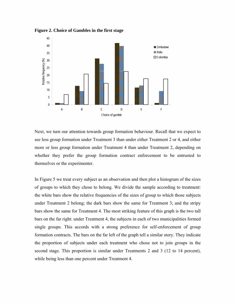
Figure 2. Choice of Gambles in the first stage

0

5

10

15

20

25

30

35

40

45

A B C D E FChoice of gamble

Relat

ive fr

eque

ncy (

%)

ZimbabweIndiaColombia

Next, we turn our attention towards group formation behaviour. Recall that we expect to

see less group formation under Treatment 3 than under either Treatment 2 or 4, and either

more or less group formation under Treatment 4 than under Treatment 2, depending on

whether they prefer the group formation contract enforcement to be entrusted to

themselves or the experimenter.

In Figure 5 we treat every subject as an observation and then plot a histogram of the sizes

of groups to which they chose to belong. We divide the sample according to treatment:

the white bars show the relative frequencies of the sizes of group to which those subjects

under Treatment 2 belong; the dark bars show the same for Treatment 3; and the stripy

bars show the same for Treatment 4. The most striking feature of this graph is the two tall

bars on the far right: under Treatment 4, the subjects in each of two municipalities formed

single groups. This accords with a strong preference for self-enforcement of group

formation contracts. The bars on the far left of the graph tell a similar story. They indicate

the proportion of subjects under each treatment who chose not to join groups in the

second stage. This proportion is similar under Treatments 2 and 3 (12 to 14 percent),

while being less than one percent under Treatment 4.

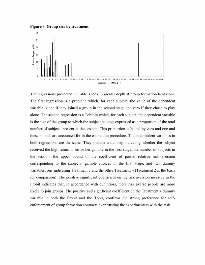
Figure 3. Group size by treatment

0

5

10

15

20

25

30

1 2 3 4 5 6 7 8 9 10 11 12 13 14 15 16 17 18 19 20 21 22 23 24 25 26 27 28 29 30 31 32 33 34 35 36 37 38 39 40 41 42 43 44 45 46Group size

Relat

ive fr

eque

ncy (

%)

T2 T3 T4

The regressions presented in Table 3 look in greater depth at group formation behaviour.

The first regression is a probit in which, for each subject, the value of the dependent

variable is one if they joined a group in the second stage and zero if they chose to play

alone. The second regression is a Tobit in which, for each subject, the dependent variable

is the size of the group to which the subject belongs expressed as a proportion of the total

number of subjects present at the session. This proportion is bound by zero and one and

these bounds are accounted for in the estimation procedure. The independent variables in

both regressions are the same. They include a dummy indicating whether the subject

received the high return to his or her gamble in the first stage, the number of subjects in

the session, the upper bound of the coefficient of partial relative risk aversion

corresponding to the subjects’ gamble choices in the first stage, and two dummy

variables, one indicating Treatment 3 and the other Treatment 4 (Treatment 2 is the basis

for comparison). The positive significant coefficient on the risk aversion measure in the

Probit indicates that, in accordance with our priors, more risk averse people are more

likely to join groups. The positive and significant coefficient on the Treatment 4 dummy

variable in both the Probit and the Tobit, confirms the strong preference for self-

enforcement of group formation contracts over trusting the experimenters with the task.

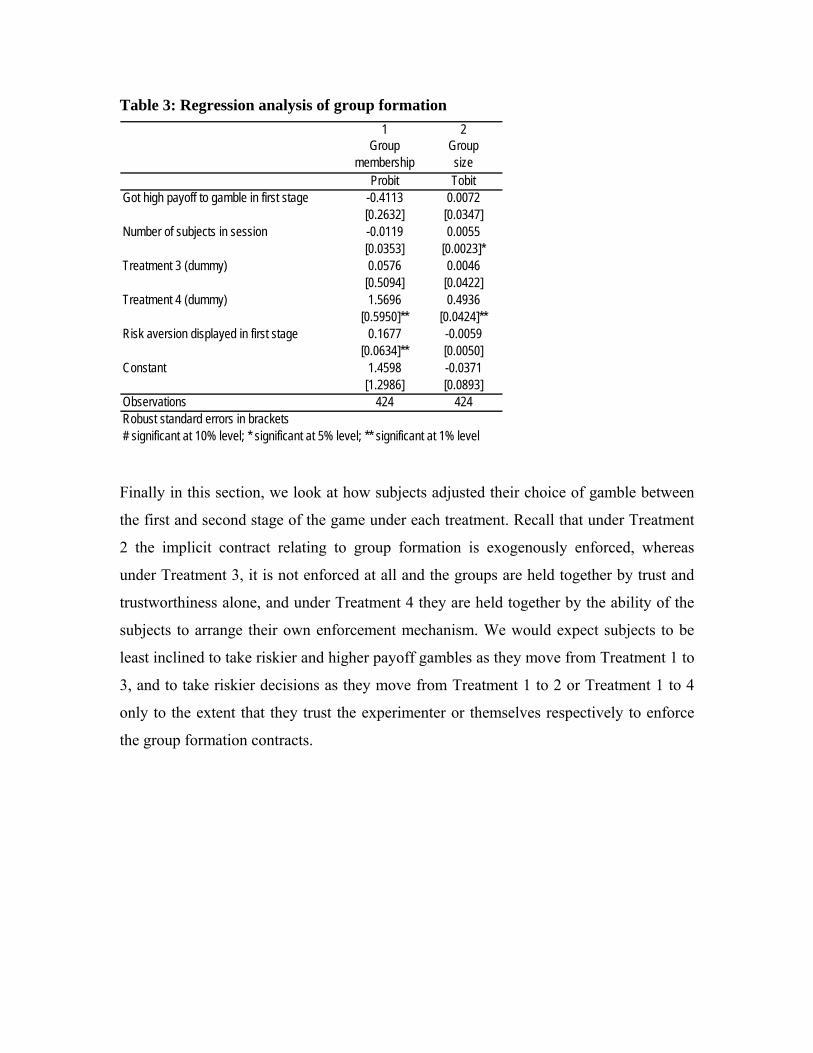
Table 3: Regression analysis of group formation 1 2

Group membership

Group size

Probit TobitGot high payoff to gamble in first stage -0.4113 0.0072

[0.2632] [0.0347]Number of subjects in session -0.0119 0.0055

[0.0353] [0.0023]*Treatment 3 (dummy) 0.0576 0.0046

[0.5094] [0.0422]Treatment 4 (dummy) 1.5696 0.4936

[0.5950]** [0.0424]**Risk aversion displayed in first stage 0.1677 -0.0059

[0.0634]** [0.0050]Constant 1.4598 -0.0371

[1.2986] [0.0893]Observations 424 424Robust standard errors in brackets# significant at 10% level; * significant at 5% level; ** significant at 1% level

Finally in this section, we look at how subjects adjusted their choice of gamble between

the first and second stage of the game under each treatment. Recall that under Treatment

2 the implicit contract relating to group formation is exogenously enforced, whereas

under Treatment 3, it is not enforced at all and the groups are held together by trust and

trustworthiness alone, and under Treatment 4 they are held together by the ability of the

subjects to arrange their own enforcement mechanism. We would expect subjects to be

least inclined to take riskier and higher payoff gambles as they move from Treatment 1 to

3, and to take riskier decisions as they move from Treatment 1 to 2 or Treatment 1 to 4

only to the extent that they trust the experimenter or themselves respectively to enforce

the group formation contracts.

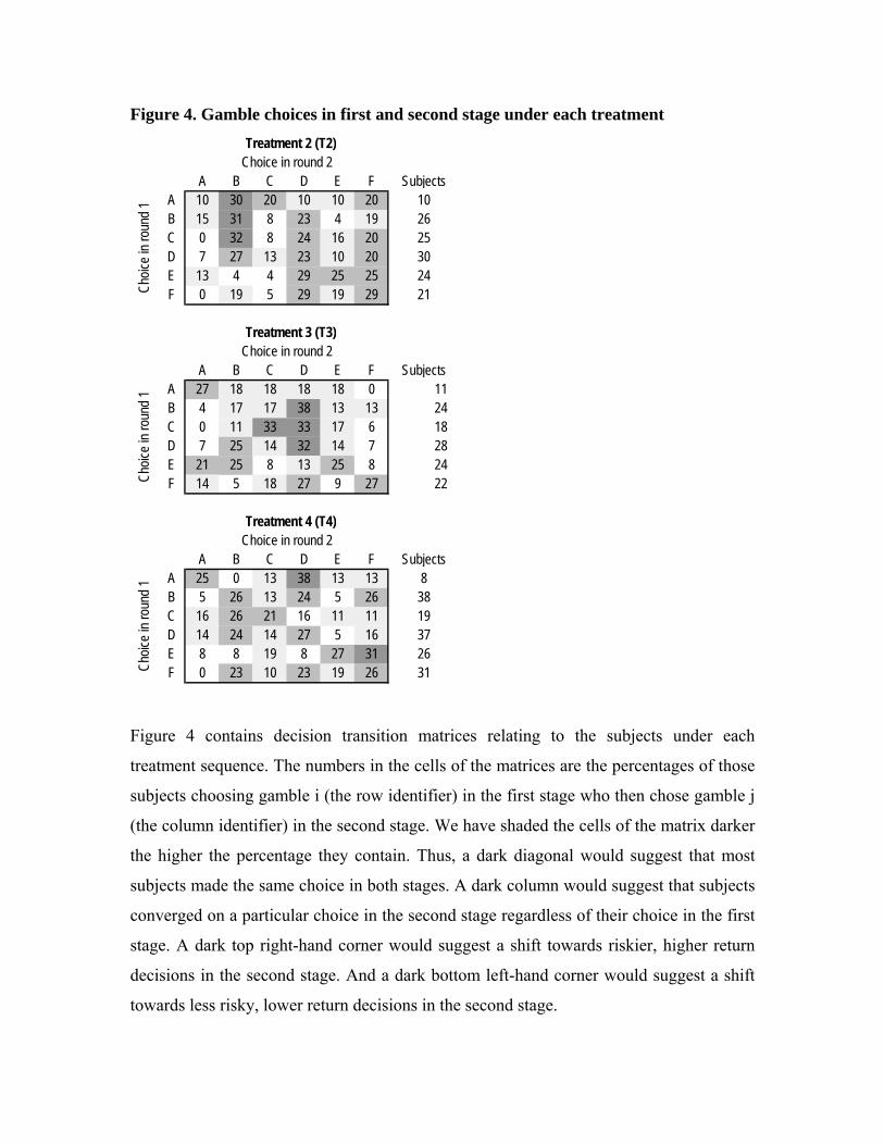
Figure 4. Gamble choices in first and second stage under each treatment Treatment 2 (T2)

A B C D E F SubjectsA 10 30 20 10 10 20 10B 15 31 8 23 4 19 26C 0 32 8 24 16 20 25D 7 27 13 23 10 20 30E 13 4 4 29 25 25 24F 0 19 5 29 19 29 21

Treatment 3 (T3)

A B C D E F SubjectsA 27 18 18 18 18 0 11B 4 17 17 38 13 13 24C 0 11 33 33 17 6 18D 7 25 14 32 14 7 28E 21 25 8 13 25 8 24F 14 5 18 27 9 27 22

Treatment 4 (T4)

A B C D E F SubjectsA 25 0 13 38 13 13 8B 5 26 13 24 5 26 38C 16 26 21 16 11 11 19D 14 24 14 27 5 16 37E 8 8 19 8 27 31 26F 0 23 10 23 19 26 31

Choice in round 2

Choice in round 2

Choic

e in r

ound

1

Choice in round 2

Choic

e in r

ound

1Ch

oice i

n rou

nd 1

Figure 4 contains decision transition matrices relating to the subjects under each

treatment sequence. The numbers in the cells of the matrices are the percentages of those

subjects choosing gamble i (the row identifier) in the first stage who then chose gamble j

(the column identifier) in the second stage. We have shaded the cells of the matrix darker

the higher the percentage they contain. Thus, a dark diagonal would suggest that most

subjects made the same choice in both stages. A dark column would suggest that subjects

converged on a particular choice in the second stage regardless of their choice in the first

stage. A dark top right-hand corner would suggest a shift towards riskier, higher return

decisions in the second stage. And a dark bottom left-hand corner would suggest a shift

towards less risky, lower return decisions in the second stage.

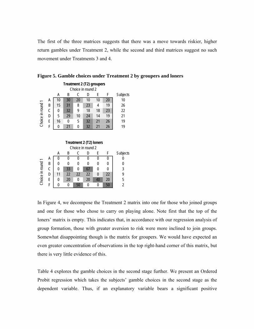
The first of the three matrices suggests that there was a move towards riskier, higher

return gambles under Treatment 2, while the second and third matrices suggest no such

movement under Treatments 3 and 4.

Figure 5. Gamble choices under Treatment 2 by groupers and loners Treatment 2 (T2) groupers

A B C D E F SubjectsA 10 30 20 10 10 20 10B 15 31 8 23 4 19 26C 0 32 9 18 18 23 22D 5 29 10 24 14 19 21E 16 0 5 32 21 26 19F 0 21 0 32 21 26 19

Treatment 2 (T2) loners

A B C D E F SubjectsA 0 0 0 0 0 0 0B 0 0 0 0 0 0 0C 0 33 0 67 0 0 3D 11 22 22 22 0 22 9E 0 20 0 20 40 20 5F 0 0 50 0 0 50 2

Choice in round 2

Choic

e in r

ound

1

Choice in round 2

Choic

e in r

ound

1

In Figure 4, we decompose the Treatment 2 matrix into one for those who joined groups

and one for those who chose to carry on playing alone. Note first that the top of the

loners’ matrix is empty. This indicates that, in accordance with our regression analysis of

group formation, those with greater aversion to risk were more inclined to join groups.

Somewhat disappointing though is the matrix for groupers. We would have expected an

even greater concentration of observations in the top right-hand corner of this matrix, but

there is very little evidence of this.

Table 4 explores the gamble choices in the second stage further. We present an Ordered

Probit regression which takes the subjects’ gamble choices in the second stage as the

dependent variable. Thus, if an explanatory variable bears a significant positive

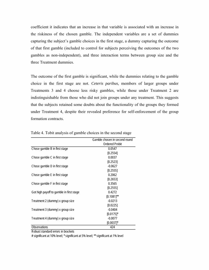
coefficient it indicates that an increase in that variable is associated with an increase in

the riskiness of the chosen gamble. The independent variables are a set of dummies

capturing the subject’s gamble choices in the first stage, a dummy capturing the outcome

of that first gamble (included to control for subjects perceiving the outcomes of the two

gambles as non-independent), and three interaction terms between group size and the

three Treatment dummies.

The outcome of the first gamble is significant, while the dummies relating to the gamble

choice in the first stage are not. Ceteris paribus, members of larger groups under

Treatments 3 and 4 choose less risky gambles, while those under Treatment 2 are

indistinguishable from those who did not join groups under any treatment. This suggests

that the subjects retained some doubts about the functionality of the groups they formed

under Treatment 4, despite their revealed preference for self-enforcement of the group

formation contracts.

Table 4. Tobit analysis of gamble choices in the second stage Gamble chosen in second round

Ordered ProbitChose gamble B in first stage 0.0547

[0.2554]Chose gamble C in first stage 0.0037

[0.2523]Chose gamble D in first stage -0.0627

[0.2555]Chose gamble E in first stage 0.2062

[0.2653]Chose gamble F in first stage 0.3565

[0.2555]Got high payoff to gamble in first stage 0.4272

[0.1081]**Treatment 2 (dummy) x group size -0.0213

[0.0225]Treatment 3 (dummy) x group size -0.0404

[0.0175]*Treatment 4 (dummy) x group size -0.0077

[0.0037]*Observations 424Robust standard errors in brackets# significant at 10% level; * significant at 5% level; ** significant at 1% level

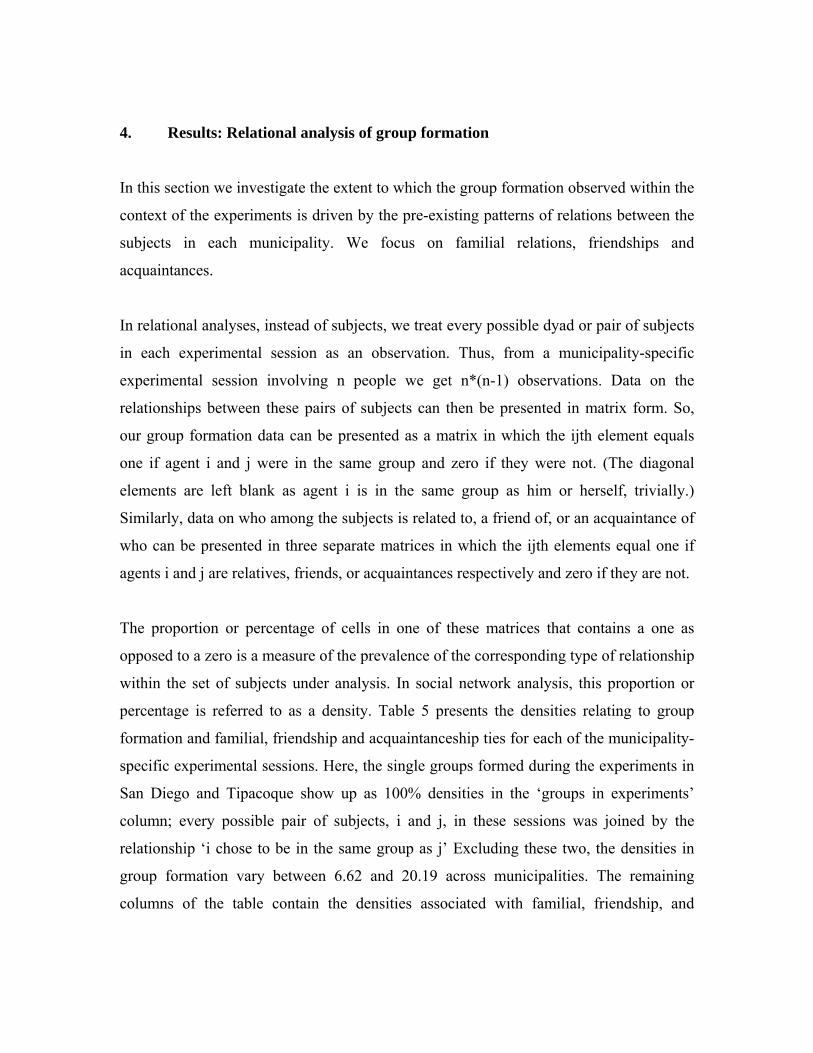
4. Results: Relational analysis of group formation

In this section we investigate the extent to which the group formation observed within the

context of the experiments is driven by the pre-existing patterns of relations between the

subjects in each municipality. We focus on familial relations, friendships and

acquaintances.

In relational analyses, instead of subjects, we treat every possible dyad or pair of subjects

in each experimental session as an observation. Thus, from a municipality-specific

experimental session involving n people we get n*(n-1) observations. Data on the

relationships between these pairs of subjects can then be presented in matrix form. So,

our group formation data can be presented as a matrix in which the ijth element equals

one if agent i and j were in the same group and zero if they were not. (The diagonal

elements are left blank as agent i is in the same group as him or herself, trivially.)

Similarly, data on who among the subjects is related to, a friend of, or an acquaintance of

who can be presented in three separate matrices in which the ijth elements equal one if

agents i and j are relatives, friends, or acquaintances respectively and zero if they are not.

The proportion or percentage of cells in one of these matrices that contains a one as

opposed to a zero is a measure of the prevalence of the corresponding type of relationship

within the set of subjects under analysis. In social network analysis, this proportion or

percentage is referred to as a density. Table 5 presents the densities relating to group

formation and familial, friendship and acquaintanceship ties for each of the municipality-

specific experimental sessions. Here, the single groups formed during the experiments in

San Diego and Tipacoque show up as 100% densities in the ‘groups in experiments’

column; every possible pair of subjects, i and j, in these sessions was joined by the

relationship ‘i chose to be in the same group as j’ Excluding these two, the densities in

group formation vary between 6.62 and 20.19 across municipalities. The remaining

columns of the table contain the densities associated with familial, friendship, and

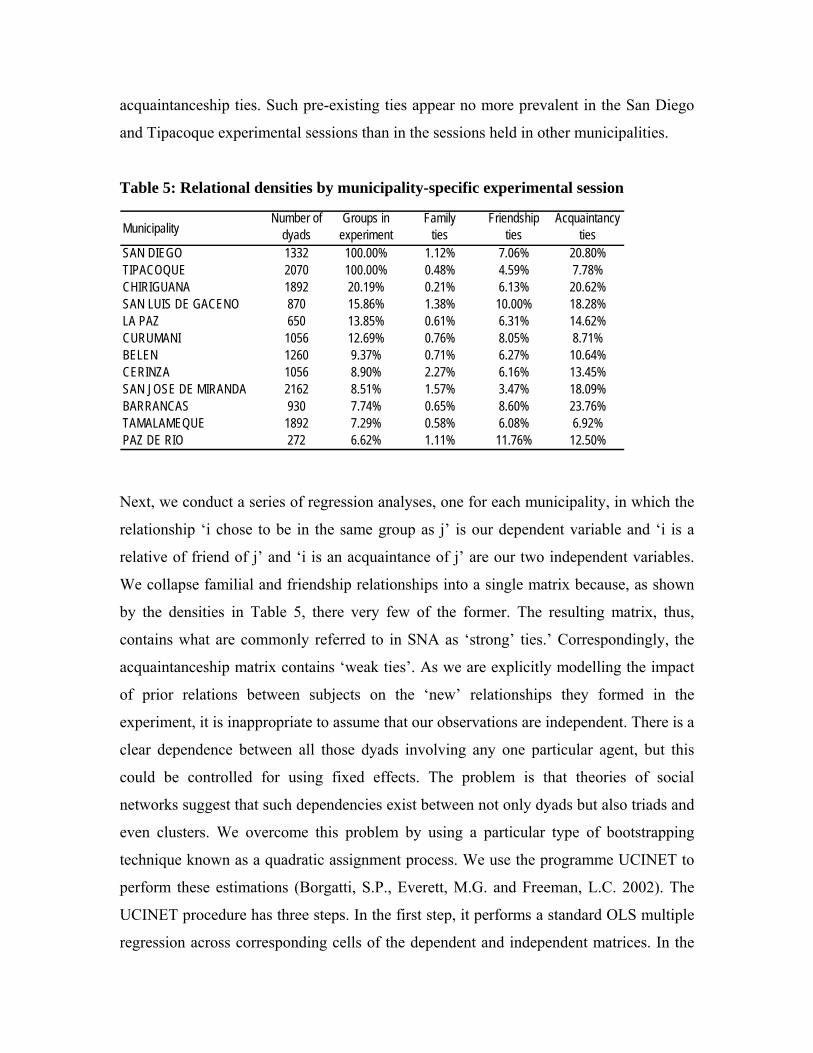
acquaintanceship ties. Such pre-existing ties appear no more prevalent in the San Diego

and Tipacoque experimental sessions than in the sessions held in other municipalities.

Table 5: Relational densities by municipality-specific experimental session

MunicipalityNumber of

dyadsGroups in

experimentFamily

tiesFriendship

tiesAcquaintancy

tiesSAN DIEGO 1332 100.00% 1.12% 7.06% 20.80%TIPACOQUE 2070 100.00% 0.48% 4.59% 7.78%CHIRIGUANA 1892 20.19% 0.21% 6.13% 20.62%SAN LUIS DE GACENO 870 15.86% 1.38% 10.00% 18.28%LA PAZ 650 13.85% 0.61% 6.31% 14.62%CURUMANI 1056 12.69% 0.76% 8.05% 8.71%BELEN 1260 9.37% 0.71% 6.27% 10.64%CERINZA 1056 8.90% 2.27% 6.16% 13.45%SAN JOSE DE MIRANDA 2162 8.51% 1.57% 3.47% 18.09%BARRANCAS 930 7.74% 0.65% 8.60% 23.76%TAMALAMEQUE 1892 7.29% 0.58% 6.08% 6.92%PAZ DE RIO 272 6.62% 1.11% 11.76% 12.50%

Next, we conduct a series of regression analyses, one for each municipality, in which the

relationship ‘i chose to be in the same group as j’ is our dependent variable and ‘i is a

relative of friend of j’ and ‘i is an acquaintance of j’ are our two independent variables.

We collapse familial and friendship relationships into a single matrix because, as shown

by the densities in Table 5, there very few of the former. The resulting matrix, thus,

contains what are commonly referred to in SNA as ‘strong’ ties.’ Correspondingly, the

acquaintanceship matrix contains ‘weak ties’. As we are explicitly modelling the impact

of prior relations between subjects on the ‘new’ relationships they formed in the

experiment, it is inappropriate to assume that our observations are independent. There is a

clear dependence between all those dyads involving any one particular agent, but this

could be controlled for using fixed effects. The problem is that theories of social

networks suggest that such dependencies exist between not only dyads but also triads and

even clusters. We overcome this problem by using a particular type of bootstrapping

technique known as a quadratic assignment process. We use the programme UCINET to

perform these estimations (Borgatti, S.P., Everett, M.G. and Freeman, L.C. 2002). The

UCINET procedure has three steps. In the first step, it performs a standard OLS multiple

regression across corresponding cells of the dependent and independent matrices. In the

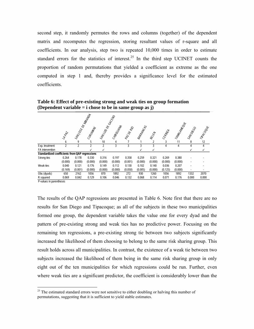
second step, it randomly permutes the rows and columns (together) of the dependent

matrix and recomputes the regression, storing resultant values of r-square and all

coefficients. In our analysis, step two is repeated 10,000 times in order to estimate

standard errors for the statistics of interest.25 In the third step UCINET counts the

proportion of random permutations that yielded a coefficient as extreme as the one

computed in step 1 and, thereby provides a significance level for the estimated

coefficients.

Table 6: Effect of pre-existing strong and weak ties on group formation (Dependent variable = i chose to be in same group as j)

LA PA

Z

SAN

JOSE

DE M

IRAN

DACU

RUMA

NI

SAN

LUIS

DE G

ACEN

OCH

IRIG

UANA

PAZ D

E RIO

BARR

ANCA

S

BELE

N

CERI

NZA

TAMAL

AMEQ

UESA

N DI

EGO

TIPAC

OQUE

6 9 5 10 4 7 1 2 3 11 8 12Exp. treatment 2 2 2 2 3 3 3 3 4 4 4 4FA interventionStandardized coefficients from QAP regressionsStrong ties 0.264 0.178 0.330 0.316 0.197 0.358 0.259 0.321 0.269 0.380 - -

(0.000) (0.000) (0.000) (0.000) (0.000) (0.001) (0.000) (0.000) (0.000) (0.000) - -Weak ties 0.040 0.121 0.176 0.149 0.112 0.130 0.102 0.140 0.036 0.207 - -

(0.169) (0.001) (0.000) (0.000) (0.000) (0.050) (0.005) (0.000) (0.125) (0.000) - -Obs (dyads) 650 2162 1056 870 1892 272 930 1260 1056 1892 1332 2070R squared 0.069 0.042 0.129 0.106 0.046 0.132 0.068 0.114 0.071 0.176 0.000 0.000P-values in parentheses

The results of the QAP regressions are presented in Table 6. Note first that there are no

results for San Diego and Tipacoque; as all of the subjects in these two municipalities

formed one group, the dependent variable takes the value one for every dyad and the

pattern of pre-existing strong and weak ties has no predictive power. Focusing on the

remaining ten regressions, a pre-existing strong tie between two subjects significantly

increased the likelihood of them choosing to belong to the same risk sharing group. This

result holds across all municipalities. In contrast, the existence of a weak tie between two

subjects increased the likelihood of them being in the same risk sharing group in only

eight out of the ten municipalities for which regressions could be run. Further, even

where weak ties are a significant predictor, the coefficient is considerably lower than the

25 The estimated standard errors were not sensitive to either doubling or halving this number of permutations, suggesting that it is sufficient to yield stable estimates.

coefficient on the strong ties. Relatives and friends are more likely to group together than

acquaintances. While the often significant coefficients on strong and weak ties suggest

that pre-existing relations had some effect on group formation in the experiment, the low

R squareds on all of the regressions suggest that they do not tell the full story.

5. Results: Combined analysis of the experimental and survey data

In this section we introduce a number of variables derived from the FA evaluation survey

into the regressions. Of primary interest to us are the effects of the FA intervention and

the ongoing violence on social capital within the municipalities. In our proposal we

predicted that direct experience of the ongoing violence is likely to increase distrust

between people and thereby reduce their willingness or ability to mobilize into groups.

The FA intervention could either crowd out social capital, as individuals become less

dependent on each other for reciprocal support in times of need and, hence, have less

reason to maintain their networks of trust, or crowd in social capital, as the various

meeting sand workshops associated with the intervention provide recipients with an

opportunity to make new acquaintances and thereby broaden their network of trust.

We identify the effect of the FA intervention by introducing a dummy variable that takes

the value one for the subjects in municipalities that are receiving the intervention and

zero otherwise. The impact of the ongoing violence is identified by introducing another

municipality-level dummy variable which, in this case, takes the value one for subjects in

municipalities where civil servants have taken labour action, we assume, because of the

threat of violence to themselves in their posting. In order to isolate any effects relating to

these variables, we also include a number of control variables in the regressions. These

include the age of the subjects, whether they are female, whether they completed primary

school, the size (number of inhabitants) of the household in which they live, household

total expenditure as a proxy for household income (entered as a natural log).

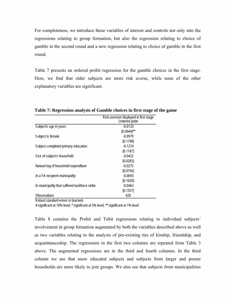
For completeness, we introduce these variables of interest and controls not only into the

regressions relating to group formation, but also the regression relating to choice of

gamble in the second round and a new regression relating to choice of gamble in the first

round.

Table 7 presents an ordered probit regression for the gamble choices in the first stage.

Here, we find that older subjects are more risk averse, while none of the other

explanatory variables are significant.

Table 7: Regression analysis of Gamble choices in first stage of the game Risk aversion displayed in first stage

Ordered pobitSubject's age in years -0.0133

[0.0044]**Subject is female -0.0979

[0.1748]Subject completed primary education -0.1274

[0.1187]Size of subject's household -0.0422

[0.0283]Natural log of household expenditure -0.0275

[0.0756]In a FA recipient municipality -0.0693

[0.1020]In municipality that suffered taskforce strike -0.0463

[0.1357]Observations 420Robust standard errors in brackets# significant at 10% level; * significant at 5% level; ** significant at 1% level

Table 8 contains the Probit and Tobit regressions relating to individual subjects’

involvement in group formation augmented by both the variables described above as well

as two variables relating to the analysis of pre-existing ties of kinship, friendship, and

acquaintanceship. The regressions in the first two columns are repeated from Table 3

above. The augmented regressions are in the third and fourth columns. In the third

column we see that more educated subjects and subjects from larger and poorer

households are more likely to join groups. We also see that subjects from municipalities

that have received the FA interventions are more likely to join groups. However, note that

our indicator of exposure to violence is absent from this regression. This is because, when

this variable (defined at the municipality-level) take the value zero (no or less violence)

all the subjects join groups; a zero in this variable is a perfect predictor of groups

formation.

This negative impact of violence on the subject’s willingness or ability to form groups

also shows up in the Tobit regression (fourth column), where the variable assumes a

negative and significant coefficient. Other effects demonstrated by the Tobit are similar

to those identified in the Probit with two exceptions. In the Tobit, a subject’s pre-existing

ties of kinship and friendship tended to suppress the size of the group they ended up

joining, presumably because of a tendency to group only with those friends and relations.

In contrast, greater numbers of prior acquaintances were associated with membership to

larger groups.

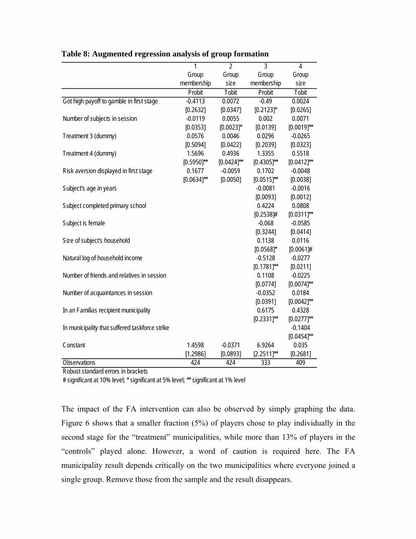
Table 8: Augmented regression analysis of group formation 1 2 3 4

Group membership

Group size

Group membership

Group size

Probit Tobit Probit TobitGot high payoff to gamble in first stage -0.4113 0.0072 -0.49 0.0024

[0.2632] [0.0347] [0.2123]* [0.0265]Number of subjects in session -0.0119 0.0055 0.002 0.0071

[0.0353] [0.0023]* [0.0139] [0.0019]**Treatment 3 (dummy) 0.0576 0.0046 0.0296 -0.0265

[0.5094] [0.0422] [0.2039] [0.0323]Treatment 4 (dummy) 1.5696 0.4936 1.3355 0.5518

[0.5950]** [0.0424]** [0.4305]** [0.0412]**Risk aversion displayed in first stage 0.1677 -0.0059 0.1702 -0.0048

[0.0634]** [0.0050] [0.0515]** [0.0038]Subject's age in years -0.0081 -0.0016

[0.0093] [0.0012]Subject completed primary school 0.4224 0.0808

[0.2538]# [0.0311]**Subject is female -0.068 -0.0585

[0.3244] [0.0414]Size of subject's household 0.1138 0.0116

[0.0568]* [0.0061]#Natural log of household income -0.5128 -0.0277

[0.1781]** [0.0211]Number of friends and relatives in session 0.1108 -0.0225

[0.0774] [0.0074]**Number of acquaintances in session -0.0352 0.0184

[0.0391] [0.0042]**In an Familias recipient municipality 0.6175 0.4328

[0.2331]** [0.0277]**In municipality that suffered taskforce strike -0.1404

[0.0454]**Constant 1.4598 -0.0371 6.9264 0.035

[1.2986] [0.0893] [2.2511]** [0.2681]Observations 424 424 333 409Robust standard errors in brackets# significant at 10% level; * significant at 5% level; ** significant at 1% level

The impact of the FA intervention can also be observed by simply graphing the data.

Figure 6 shows that a smaller fraction (5%) of players chose to play individually in the

second stage for the “treatment” municipalities, while more than 13% of players in the

“controls” played alone. However, a word of caution is required here. The FA

municipality result depends critically on the two municipalities where everyone joined a

single group. Remove those from the sample and the result disappears.

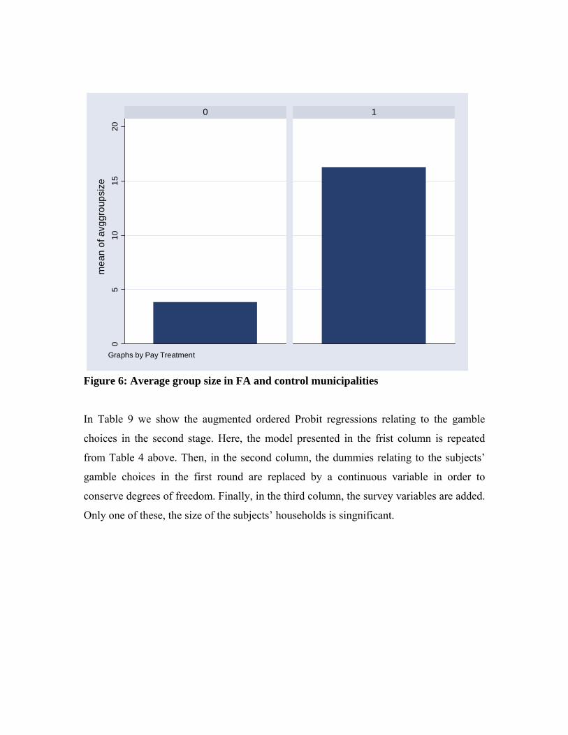
Figure 6: Average group size in FA and control municipalities

In Table 9 we show the augmented ordered Probit regressions relating to the gamble

choices in the second stage. Here, the model presented in the frist column is repeated

from Table 4 above. Then, in the second column, the dummies relating to the subjects’

gamble choices in the first round are replaced by a continuous variable in order to

conserve degrees of freedom. Finally, in the third column, the survey variables are added.

Only one of these, the size of the subjects’ households is singnificant.

05

1015

200 1

mea

n of

avg

grou

psiz

e

Graphs by Pay Treatment

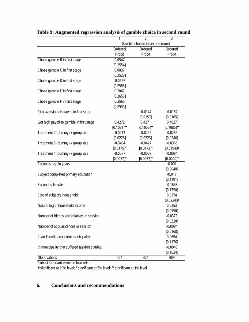
Table 9: Augmented regression analysis of gamble choice in second round 1 2 3

Gamble chosen in second roundOrdered Probit

Ordered Probit

Ordered Probit

Chose gamble B in first stage 0.0547[0.2554]

Chose gamble C in first stage 0.0037[0.2523]

Chose gamble D in first stage -0.0627[0.2555]

Chose gamble E in first stage 0.2062[0.2653]

Chose gamble F in first stage 0.3565[0.2555]

Risk aversion displayed in first stage -0.0144 -0.0157[0.0157] [0.0165]

Got high payoff to gamble in first stage 0.4272 0.4271 0.4027[0.1081]** [0.1055]** [0.1085]**

Treatment 2 (dummy) x group size -0.0213 -0.0222 -0.0236[0.0225] [0.0223] [0.0246]

Treatment 3 (dummy) x group size -0.0404 -0.0427 -0.0368[0.0175]* [0.0173]* [0.0194]#

Treatment 4 (dummy) x group size -0.0077 -0.0078 -0.0084[0.0037]* [0.0037]* [0.0040]*

Subject's age in years -0.001[0.0048]

Subject completed primary education -0.017[0.1191]

Subject is female -0.1658[0.1750]

Size of subject's household 0.0374[0.0224]#

Natural log of household income 0.0253[0.0950]

Number of friends and relatives in session -0.0373[0.0320]

Number of acquaintances in session -0.0084[0.0168]

In an Familias recipient municipality 0.0694[0.1176]

In municipality that suffered taskforce strike -0.0046[0.1624]

Observations 424 424 409Robust standard errors in brackets# significant at 10% level; * significant at 5% level; ** significant at 1% level

6. Conclusions and recommendations

The results presented above suggest that the pilot was a success. That the gamble choice

in the first stage of the game is associated with the age of the subject in a way that is

corroborated with other studies is heartening. That the gamble choice (converted into

levels of risk aversion) then predicts who chooses to go into a group is also encouraging.

The group formation within the context of the experiment can be explained with

considerable success when analysed in conjunction with the survey data. Some caution is

required when drawing conclusions relating to the impact of the FA intervention and

violence, primarily because both of these variables are defined at the municipality- rather

than the individual subject-level. However, the sign, size and apparent robustness of the

coefficients on these variables is very encouraging.

Our results suggest that the FA intervention has crowded in social capital, that violence

undermines social capital, and that the campesions in our sample have a strong preference

for enforcing informal contracts made among themselves by themselves rather than by an

experimenter, i.e., an apparently benevolent stranger in their midst.