Displacement Following of Hidden Objects in a Video Sequence

International Journal of Computer Vision 57(2), 91–105, 2004c© 2004 Kluwer Academic Publishers. Manufactured in The Netherlands.

Displacement Following of Hidden Objects in a Video Sequence

OLIVIA SANCHEZ AND FRANCOISE DIBOSCEREMADE, Universite Paris IX-Dauphine, Place du Marechal de Lattre de Tassigny,

75775 Paris, Cedex 16, [email protected]

[email protected]

Received June 29, 2001; Revised March 14, 2003; Accepted June 2, 2003

Abstract. In a video sequence, computing the motion of an object requires the continuity of the apparent velocityfield. This property does not hold when the object is hidden by an occlusion during its motion. The minimizationof an energy functional leads to a simple algorithm which allows the recovery of the most likely trajectory of theoccluded object from optical flow data at the border of the occlusion. Optical flow used for developing our methodis an improvement on any variational technique of computing it. This improvement is based on a multichannelsegmentation.

Keywords: motion estimation, optical flow, segmentation, occlusion, variational methods

1. Introduction

Occlusions occurrence in a video sequence is a frequentphenomenon generated by the natural superposition ofseveral objects in the scene. In 3D scene, due to relativedepth, an object close to the visual sensor can hideanother object further away (see Fig. 1).

We can distinguish several occlusion categorieswhich produce some problems with a different algorith-mic treatment. Their classification may be establishedby taking into account two criteria. The first one is thedynamic or the static nature of the objects involvedin occlusion phenomenon. The second one consists ofknowing whether the occlusion is partial or total, thatis to say if a part of the occluded region remains visibleor completely disappears under the occluding region.In our work, we explored the case when the occludedobject moves and the occluding object may be fixedor move on a fixed background. In addition, occlusionmay be total.

In this case, the human eye is able to extract relevantvisual information from the occluded object when itdisappears and it becomes visible again; and then to

reconstruct its displacement. The aim of this article isto recover the most probable motion followed by thehidden object with the motivation to replicate this basiccapacity of our visual perception.

In order to do this, we have proposed a comple-mentary work (Sanchez, 2002): a novel method forthe automatic determination of the occluding and theoccluded objects. This practical technique permits usto know the location of the occluding object (in mo-tion). In the vicinity of the boundary of the occlud-ing object, we write the recovering of the occludedobject displacement as an interpolation based on themotion.

Indeed, recovering the trajectory of the occluded ob-ject in an active scene requires motion estimation. Anuseful mathematical tool to estimate motion in a videosequence is optical flow. Optical flow is the velocityprojection of real objects onto the image plane. Thisprojection is generally the velocities field described byintensity changes in the video sequence. Phenomenasuch as shading effects, reflections or noise can lead tosome changes in image brightness which do not corre-spond to real motion; however, in most cases, optical

92 Sanchez and Dibos

A

A

A

B B B

A

A

B

B

B

B

B

B

A

A

A

Figure 1. Above, a fixed object, B, and A which moves in the first diagonal line in three-dimension. If we consider the projection of this sceneonto the image plane, we can see that, in the intermediate frame, the position of the object A is hidden by object B.

flow can be interpreted as a reliable approximation ofmotion.

The necessity of having the optical flow at one’s dis-posal does not lead us to present a new method forits computation. We only need a coherent optical flow.Thus, we have improved it by a multichannel segmen-tation associated with an average process. Then, theoptical flow data over the whole sequence allows us todetermine the trajectory of the hidden object even ifit is entirely concealed by the occluding object. Thistrajectory is computed as the minimizer of an energyfunctional. This functional involves the configurationsof the angles made by the optical flow vectors aroundthe occluding object.

This paper is divided into four sections. The firstsection is devoted to a survey of a few representativemethods about optical flow estimation by variationaltechniques. In the second section, we propose an im-provement of the variational methods which allows usto obtain a good approximation of the optical flowaround the occluding object border. We describe themethod which leads to the recovered trajectories in thethird section. Finally, the last section illustrates our ap-proach by experiments on synthetic and real sequences.

2. A Few Techniques to Compute Optical Flow

Optical flow measure is a very active topic of researchin image analysis, and a lot of methods have been pro-posed to determine it. A performance comparison ofthe main techniques has been realized in Barron et al.

(1994). In this section, we present a few variationalmethods. This type of approach consists of minimiz-ing an energy functional which contains two terms. Thefirst term is a term which is computed from the bright-ness intensity, and the second one is a smoothing term.

Let I (x, y, t) be the intensity brightness at point(x, y) ∈ �t ⊂ R

2, �t is the rectangular image domainat the time t ∈ [0, T ], T > 0.

A very common requirement to compute optical flowis to assume that a point keeps a constant intensityduring its displacement

d I

dt= 0, (1)

which leads to the following equation called the opticalflow constraint

Ix · u + Iy · v + It = 0 (2)

where u and v are the velocity components of the ap-parent motion. The only component which can be de-duced by this equation is the normal component of thevelocity field in the direction of the brightness gradient(Ix , Iy). It can be written as

σn = −It (x, y, t)∇ I (x, y, t)

‖∇ I (x, y, t)‖2 . (3)

We need another constraint to get unicity of u and v. Itis the aperture problem. As part of the variational tech-niques, the second constraint corresponds to a smooth-ing of the velocity field.

Displacement Following of Hidden Objects in a Video Sequence 93

To determine (u, v), one minimizes the functional

E(u, v) =∫

�

((Ix · u + Iy · v + It )2 + α(φ(‖∇u‖)

+ φ(‖∇v‖)) dx dy, (4)

where the function φ characterizes the smoothing andα is a weight which controls the influence of this term.The Euler-Lagrange equations are a system of two dif-ferential equations

div

(φ′(‖∇u‖)

‖∇u‖ · ∇u

)− 1

αIx (Ix u + Iyv + It ) = 0

div

(φ′(‖∇v‖)

‖∇v‖ · ∇v

)− 1

αIy(Ix u + Iyv + It ) = 0

(5)

where φ′ is the derivative of φ with respect to its ar-gument and div is the 2D divergence operator div =∂x + ∂y .

If η is the gradient direction and ξ the normal direc-tion to η, then the divergence term can be decomposedas

div

(φ′(‖∇u‖)

‖∇u‖ .∇u

)= φ′(‖∇u‖)

‖∇u‖ uξξ + φ′′(‖∇u‖)uηη,

(6)

where uξξ (respectively uηη) is the second order deriva-tive in the directional ξ (respectively η). We obtainsimilar expressions for v.

• A first approach (see Horn and Schunck, 1981) con-sists of compelling the velocity field to vary smoothlyin space. So the choice of φ is φ(‖∇u‖) = ‖∇u‖2.The weights associated to uξξ and uηη are the same:it is an isotropic smoothing. As a consequence, thisregularity constraint induces an undesirable smooth-ing across the motion discontinuities and thereforedoes not allow to recover the velocity in the border ofmoving objects edges. Indeed, this constraint impliesthat all points considered for smoothing the velocityfield belong to the same object. But, this is not valid atthe boundaries of rigid objects with independent mo-tions, or at the different areas of a same jointed object.

To avoid this problem, several techniques for es-timating optical flow by managing discontinuitiesexist (refer to the good survey (Orkisz and Clarysse,1996), and also (Alvarez et al., 1999, 2000; Nesi,1993). The usual process is to find a function φ whichboth smoothes the optical flow inside homogeneous

regions (characterized by a weak gradient), and pre-serves the flow discontinuities in inhomogeneous re-gions (where the gradient is strong). The smoothingcondition inside homogeneous regions expresses it-self in equal limits for uξξ and uηη weights when thegradient is weak (‖∇u‖ → 0), whereas the limitedsmoothing condition across discontinuities amountsto cancel the weight along the gradient directionwhen the latter is strong (‖∇u‖ → ∞). These twoconditions cannot be realized simultaneously, so weimpose a swifter diffusion in the gradient directionη than in the direction ξ (see Deriche and Faugeras,1995).

• The optical flow gradient norm squared can be re-placed by some total variation measures. Then wechoose φ(‖∇u‖) = ‖∇u‖. Only the weight in thedirection perpendicular to gradient is not zero. Thatis the case of an anisotropic smoothing. From denois-ing techniques by total variation, a first work (Cohen,1993) has proposed to use a minimization based onthe L1 norm. With the same type of minimization,in (Kumar et al., 1996) the estimation problem ofoptical flow is considered as a curve evolution prob-lem. This technique of non quadratic regularizationhas also been developed in Cohen and Herlin (1999)with a non uniform multi-resolution, in order to in-crease the numerical accuracy of the solution in thestudied regions. A rigorous analysis of this problemhas been realized (see Aubert et al., 1999). Whenthe constraint is written as a total variation mea-sure, these authors show that if the data I is regu-lar (lipschitz), this problem is well-posed in space ofbounded variation functions BV (�) (this is not thecase if I is of bounded variations). They provide a nu-merical scheme (half quadratic minimization) whichconverges to the unique solution of this problem.

• The improvement of the memory storage capacity ofthe present computer tools permits to treat the wholevideo sequence. Based on this remark, a spatio-temporal smoothing has been proposed in Weickertand Schnorr (2001). Whereas most of the optical flowcomputation methods work locally in time, insofaras only two frames are used for recovering it, theseauthors exploit the temporal intrinsic coherence ofa sequence by proposing to minimize the followingenergy

E(u, v) =∫

�×[0,T ]((Ix · u + Iy · v + It )

+ α�(|∇θu|2 + |∇θ v|2)) dx dy dt, (7)


where ∇θ = (∂x , ∂y, ∂t ) is the spatio-temporal op-erator ∇.

The minimization of this functional is a convexand non-quadratic optimization problem; it has anunique minimum which is determined by a gradientdescent algorithm.

3. Optical Flow Estimation via a Segmentation

There are alternative assumptions to the Eq. (2) but noassumption allows an exact determination of opticalflow. Insofar as only an adequate estimation for ourulterior work is required, our method will not be topropose a new functional to minimize. Our approachconsists of replacing an initial optical flow by a piece-wise constant optical flow which is well adapted toour purpose of trajectories reconstruction. This piece-wise constant optical flow is obtained by a multichannelsegmentation of the successive images of the video se-quence, and then an average. In our experiments, wehave used the optical flow given by different methods.The obtained improvements are roughly similar. Wemay note that we may use the Horn-Schunck method,which is simple and fast, because the segmentation op-eration partly allows us to avoid the smoothing problemacross the discontinuities motion.

Segmentation Method

In order to improve the optical flow given by a varia-tional method, we propose the use of a multichannelsegmentation. At the beginning, this kind of segmenta-tion has been presented for texture discrimination. Tothe best of our knowledge, it has not been used for im-proving the segmentation of moving objects in a videosequence.

First, let us recall the approach of Mumford and Shahsegmentation (see Mumford and Shah, 1989) in grayvalue image case.

We consider a simplified expression of Mumford andShah functional:

E(K ) =∫

�\K| f − g|2 dx dy + λl(K ). (8)

The first term represents the quadratic distance betweenthe images g and f where g is the picture defined on anopen rectangle �, f is a piecewise constant functionwhich aims to approximate g, K is the set of boundarieswith total length l(K ). The real parameter λ is a weight

on the length of boundaries: the high values of λ tendto reduce l(K ), whereas the small values allow a lotof boundaries. The algorithm which leads to the mini-mization of this functional has been implemented witha region growing method (see Koepfler et al., 1993).The initial picture is partitioned in squares and theirsize is to be specified by the user. The algorithm makesthe energy (8) decrease by merging some regions of thepicture. The decision to proceed to the merging of twoadjacent regions Oi and O j depends on the sign of:

E(K\∂(Oi O j )) − E(K ) = |Oi | · |O j ||Oi | + |O j | | f i − f j |2

−λ.l(∂(Oi , O j )) (9)

where | · | designs the surface measure and f i , f j arerespectively the mean values of g on the regions Oi etO j . We choose f k = 1

|Ok |∫

Okg, k is i or j .

Now, let us briefly present the extension of this al-gorithm with a multichannel datum.

In this case, g is a vector valued function from R2 to

Rn , n denoting the number of considered channels.The departure image is

g =

g1

g2

...gn

and the result image

f =

f1

f2

...

fn

.

The quadratic distance is a weighted norm by p =(p1, p2, . . . , pn), pi , i ∈ [1, . . . , n], are the weightsassociated to each channels:

| f − g|2 = dist( f, g) =n∑

i=1

pi · ( fi − gi )2 (10)

This multichannel segmentation algorithm allows usto find for a given λ an approximation of g by thepiecewise constant function f . More precisely, thismethod does not compute exactly the global minimumbut provides a quite good approximation (see Moreland Solemini, 1994).


For our optical flow segmentation, we use the mul-tichannel segmentation, described above, in which thedifferent channels are chosen as following:

• The gray level, which permits to determine the mov-ing or static objects insofar as they correspond tomore or less homogeneous regions from a photo-metric view.

• The direction of optical flow computed by a varia-tional method. This channel could improve the seg-mentation when the differences of gray levels do notcorrespond to physical objects. Then, the character-ization of a moving object could be obtained by theorientations of its optical flow vectors, if these areclose. The angles are defined in [0, 2π ] and the com-parison criterion between two angles αi and α j isMin(|αi − α j |, 2π − |αi − α j |).

• The norm of optical flow vectors which could helpto distinguish the different objects by the intensityof their respective velocity.

The choice of the pi parameters depends on the stud-ied video sequence. In a general way, the parametersassociated to the level gray is favored when the ob-jects are rigid, homogeneous and their motions can bedescribed by some translations. Fluid objects, rotatingmotions cases require a larger weight for the motioncriteria.

Optical flow average

In order to obtain a well adapted data of the optical flow,our method is then based on the fact that all pointsforming a region correspond to a location where theoptical flow is expected to be uniform.

In most cases, a choice which appears to be coher-ent is to associate to the points belonging to the sameregion the same velocity vector. This velocity vector isthe average of the optical flow vectors over this regionstemmed from multichannel segmentation.

We illustrate the behavior of this method on sev-eral sequences. We have considered two real-image se-quences. The first one is the famous Hambourg taxisequence (see Figs. 2–7), and the second one repre-sents an active region loops on sun surface provided bythe ROB (Royal Observatory of Belgium) (see Figs.8–11).

Moreover, we give a result on a sequence with arotational motion (see Figs. 12 and 13).

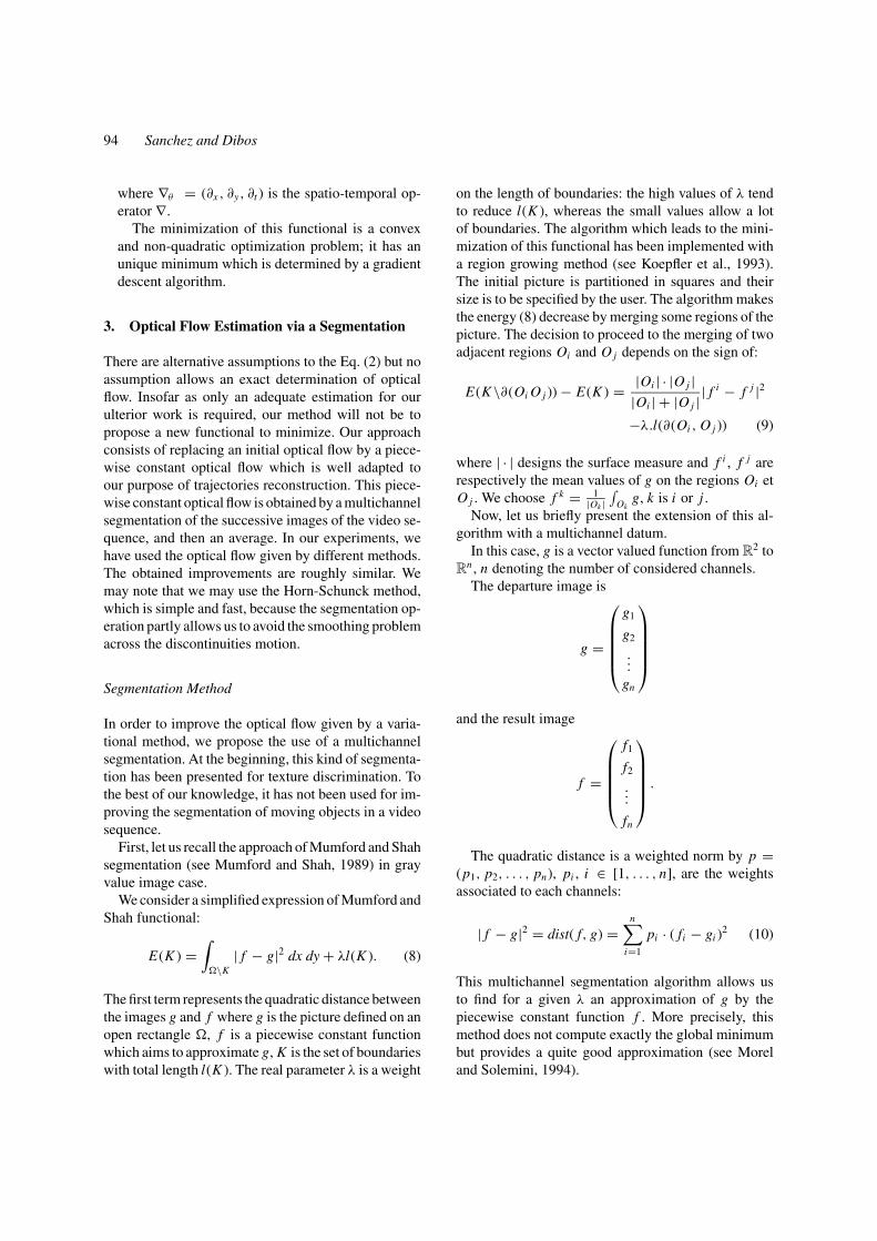
Figure 2. Hambourg taxi sequence. In this real scene, four objectsmove: at the foreground a car going from the left to the right, a vanfrom the right to the left, a clear taxi turns to the cross street and apedestrian walks at the left top.

4. Description of a Method to Recoverthe Trajectory of the Occluded Object

4.1. Motivation

In the case of an image, to resolve the disocclusionproblem, two approaches have been developed: in-painting (see Bertalmio et al., 2000), Filling-in (seeBallester et al., 2001) methods and level lines method(see Masnou and Morel, 1998). This algorithm pro-posed in Masnou and Morel (1998) solves an inter-polation problem with boundary conditions inspiredby a fundamental process of the visual perception: theamodal completion. This process characterizes the ca-pacity of our visual system to recover the hidden partof an object by artificially extending its boundaries.

For an images sequence, in the same way, the hu-man eye is able to recover the hidden object trajectorywhen enough information associated to this object areavailable. Let us specify what kind of informations areneeded.

An occlusion phenomenon between two objects inan images sequence, takes place on several consecutiveimages by following a precise scenario. This scenariostands out in two main stages. The first one is the par-tial phase of covering. The occluded object disappearsgradually under the occluding object. The second oneis the uncovering when the occluded object re-appearsgradually. Between these two stages, the occluded ob-ject may completely disappear. Figure 14 illustratesthese different stages.

In order to recover the motion of the occluded ob-ject, the human eye needs to know both about the cov-ering and the uncovering stage. So we consider the


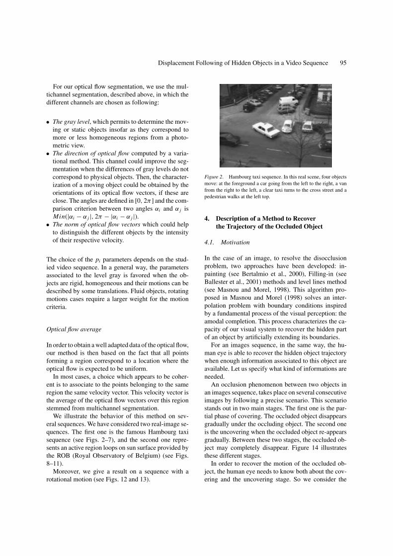
Figure 3. On the left, the direction of optical flow vectors and the right its norm. This optical flow has been computed by the Horn-Schunckmethod. We can distinguish three homogeneous regions from these two channels. They correspond to the three main moving objects in thissequence.

Figure 4. On the left, we can see a segmentation using only gray levels and on the right the segmentation using the three channels: the gray level(weight by 0.3), optical flow vectors direction (0.1) and its norm (0.6) from the Fig. 3. We can see an improvement of the segmentation resultinsofar as the car at the foreground and the van are detected with the multichannel segmentation. It is not the case with the first segmentationbecause the gray levels associated to these two objects do not allow to characterize them from the fixed background.

Figure 5. On the left, the optical flow with the Horn-Schunck method (100 iterations α = 1) and on the right, the optical flow with theWeickert-Schnorr technique (see Weickert and Schnorr, 2001).

video sequences with these two stages. In this case (seeFig. 15), we may observe that:

• On the first frames which correspond to the coveringstage, there is a vectors optical flow field associatedto the occluded object which “goes” into the occlud-ing object.

• On the next frames which correspond to the uncov-ering stage, there is a vectors optical flow field as-

sociated to the occluded object which “goes” out ofthe occluding object.

We try to associate these two optical flows to recoverthe displacement of the hidden object. To do this, wepropose a representation of these optical flows whichpermits us to write our problem like a interpolationproblem close to Masnou and Morel (1998).


Figure 6. On the left, the result with the optical flow vectors average on the 100 regions stemmed from the multichannel segmentation whenthe input is the optical flow obtained by the Horn-Schunck method. The segmentation has been realized by using the level gray intensity criterion(weighted by 0.7), the direction of optical flow (0.1) and the norm of optical flow (0.2). For a better visibility, only the vectors with a norm > 0.5have been represented. On the right, the picture shows the result of the multichannel method with the optical flow given by the Weickert-Schnorrtechnique.

Figure 7. The same results onto the real image.

Figure 8. An image of a solar active region. Solar active regionsare the areas of the sun where magnetic flux has erupted. This createssome loops where the coronal mass is ejected. The aim is to segmentthese different loops which are fluids. The motion rises at the bright-ening region (at the right top) and goes to the bottom of the imagefollowing the different loops.

4.2. A Well-Adapted Representationof the Optical Flow

Let us denote by Ut the occluding object detected onthe studied movie at the time t and �t its boundary.

We suppose that this occlusion is simply connected,and of the first order, in other words, objects hiddenby this occlusion do not occlude themselves anotherobjects.

We consider the situation where the occluded andoccluding objects are in motion. So each generatesa different optical flow. Our proposal is the follow-ing: to compute the optical flow of the occluded ob-ject at the border of the occlusion, and then to findthe trajectories followed by this object undergoingthe occlusion. The first problem is to obtain a reli-able optical flow associated to the occluded object.At the border of the occlusion, the optical flow cor-responds to a mixture between the optical flow of theoccluded and the occluding objects. But thanks to ourmultichannel segmentation method, and the precau-tion to take a slightly dilated occlusion, we guaran-tee to have, in most of the configurations, a reliabledatum of the optical flow associated to the occludedobject.

Then, to get reliable values of the optical flow associ-ated to the occluded object, we define a new occlusion


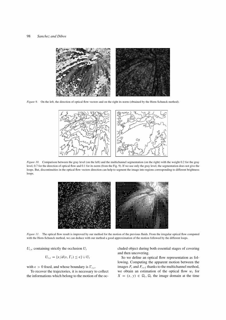
Figure 9. On the left, the direction of optical flow vectors and on the right its norm (obtained by the Horn-Schunck method).

Figure 10. Comparison between the gray level (on the left) and the multichannel segmentation (on the right) with the weight 0.2 for the graylevel, 0.7 for the direction of optical flow and 0.1 for its norm (from the Fig. 9). If we use only the gray level, the segmentation does not give theloops. But, discontinuities in the optical flow vectors direction can help to segment the image into regions corresponding to different brightnessloops.

Figure 11. The optical flow result is improved by our method for the motion of the previous fluids. From the irregular optical flow computedwith the Horn-Schunck method, we can deduce with our method a good approximation of the motion followed by the different loops.

Ut,ε containing strictly the occlusion Ut

Ut,ε = {x/d(x, �t ) ≤ ε} ∪ Ut

with ε > 0 fixed, and whose boundary is �t,ε .To recover the trajectories, it is necessary to collect

the informations which belong to the motion of the oc-

cluded object during both essential stages of coveringand then uncovering.

So we define an optical flow representation as fol-lowing. Computing the apparent motion between theimages Ft and Ft+1 thanks to the multichannel method,we obtain an estimation of the optical flow wt forX = (x, y) ∈ �t , �t the image domain at the time


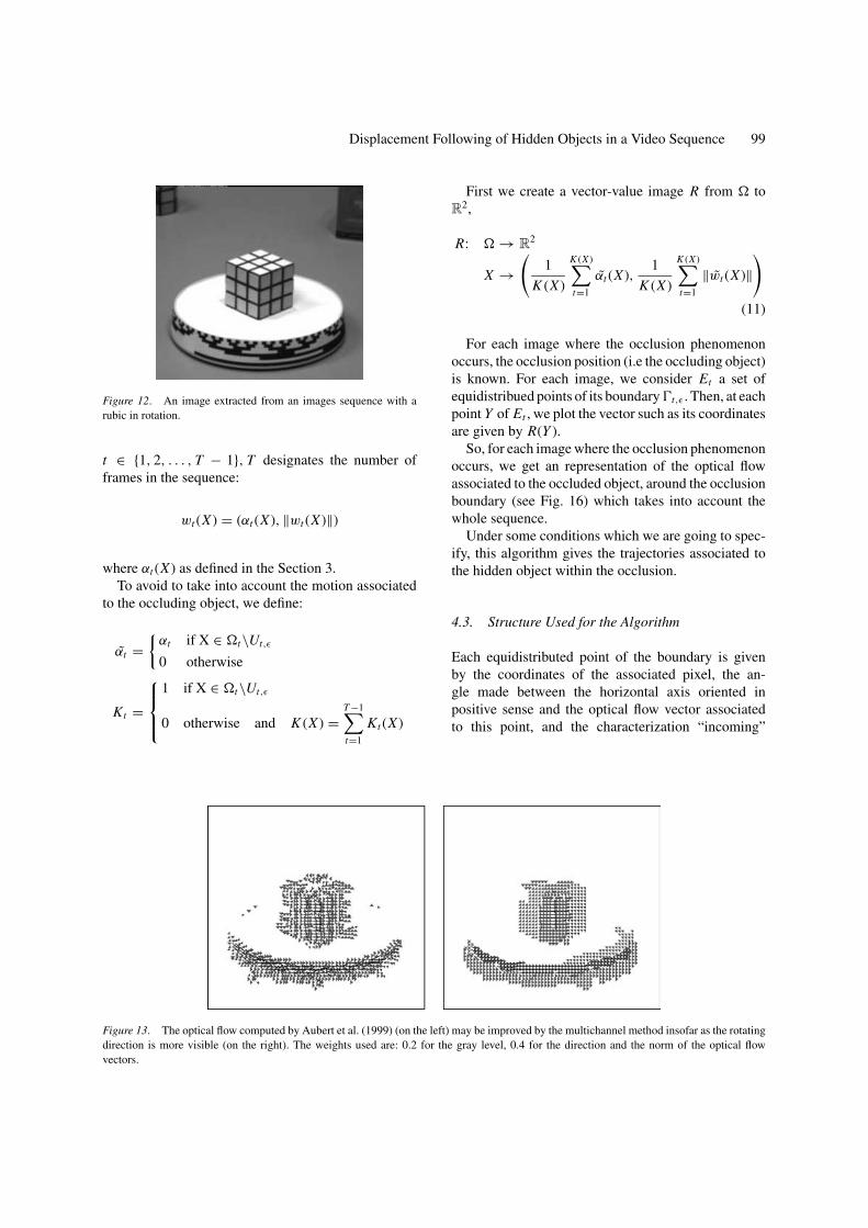
Figure 12. An image extracted from an images sequence with arubic in rotation.

t ∈ {1, 2, . . . , T − 1}, T designates the number offrames in the sequence:

wt (X ) = (αt (X ), ‖wt (X )‖)

where αt (X ) as defined in the Section 3.To avoid to take into account the motion associated

to the occluding object, we define:

αt ={

αt if X ∈ �t\Ut,ε

0 otherwise

Kt =

1 if X ∈ �t\Ut,ε

0 otherwise and K (X ) =T −1∑t=1

Kt (X )

Figure 13. The optical flow computed by Aubert et al. (1999) (on the left) may be improved by the multichannel method insofar as the rotatingdirection is more visible (on the right). The weights used are: 0.2 for the gray level, 0.4 for the direction and the norm of the optical flowvectors.

First we create a vector-value image R from � toR

2,

R: � → R2

X →(

1

K (X )

K (X )∑t=1

αt (X ),1

K (X )

K (X )∑t=1

‖wt (X )‖)

(11)

For each image where the occlusion phenomenonoccurs, the occlusion position (i.e the occluding object)is known. For each image, we consider Et a set ofequidistribued points of its boundary �t,ε . Then, at eachpoint Y of Et , we plot the vector such as its coordinatesare given by R(Y ).

So, for each image where the occlusion phenomenonoccurs, we get an representation of the optical flowassociated to the occluded object, around the occlusionboundary (see Fig. 16) which takes into account thewhole sequence.

Under some conditions which we are going to spec-ify, this algorithm gives the trajectories associated tothe hidden object within the occlusion.

4.3. Structure Used for the Algorithm

Each equidistributed point of the boundary is givenby the coordinates of the associated pixel, the an-gle made between the horizontal axis oriented inpositive sense and the optical flow vector associatedto this point, and the characterization “incoming”


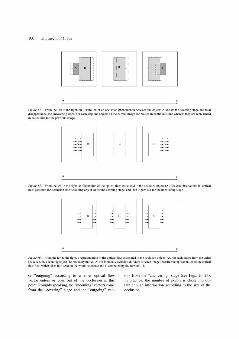
Figure 14. From the left to the right, an illustration of an occlusion phenomenon between the objects A and B: the covering stage, the totaldisappearance, the uncovering stage. For each step, the objects on the current image are plotted in continuous line whereas they are representedin dotted line for the previous image.

t0 T

A B BB A

Figure 15. From the left to the right, an illustration of the optical flow associated to the occluded object (A). We can observe that its opticalflow goes into the occlusion (the occluding object B) for the covering stage, and then it goes out for the uncovering stage.

t0 T

B B B

Figure 16. From the left to the right, a representation of the optical flow associated to the occluded object (A). For each image from the videosequence, the occluding object (B) boundary moves. At this boundary (which is different for each image), we draw a representation of the opticalflow field which takes into account the whole sequence and is computed by the formula 11.

or “outgoing” according to whether optical flowvector enters or goes out of the occlusion at thispoint. Roughly speaking, the “incoming” vectors comefrom the “covering” stage and the “outgoing” vec-

tors from the “uncovering” stage (see Figs. 20–23).In practice, the number of points is chosen to ob-tain enough information according to the size of theocclusion.


By covering the boundary of occlusion in anti-trigonometric direction, we obtain an arranged list.

4.4. Constraints Linked with the Recovery Problemof the Trajectories at Occlusion Boundary

The recovery of the trajectories which pass through theconsidered points of the occlusion boundary consistsof matching these admissible points. This is done byminimizing the length of their connected paths and acoefficient depending of the incident and outgoing an-gles of these points.

Four constraints must be enforced to obtain an ac-curate optical flow restoration:

1. To define some permissible trajectories within theocclusion, each optical flow vector “incoming” inthe occlusion has a corresponding optical flow vec-tor (if it exists) which necessarily goes out of theocclusion. Hence, it is essential to allow to connectonly two points if they have a complementary po-sition (association “incoming” with “outgoing” andreciprocally) with respect to the occlusion.

2. Two trajectories connecting two pairs of points can-not intersect themselves. Indeed, these trajectoriesdefine the motions of some objects hidden by theocclusion which cannot overlap because we haveassumed that this occlusion was of the first order.This second constraint induces a causality principleuseful for putting in connection these points. We de-note J the set of N points of the detected occlusionarranged in anti-trigonometric sense. Indeed, whentwo points jl and jl ′ are connected, the set J is con-stituted by these two points and by the two subsetsJ 1 and J 2 such that if we consider that l < l ′:

J = { j1, j2, . . . , jl , . . . , jN }= { jm/m ∈ [l, l ′]} ∪ { jl+1, . . . , jl ′−1}

∪ { jl} ∪ { jl ′ }= J 1 ∪ J 2 ∪ { jl} ∪ { jl ′ }

where J 1 = { jm/m /∈ [l, l ′]} and

J 2 =

{ jl+1} = { jl ′−1} if l ′ = l + 2

∅ if l ′ = l + 1

{ jl+1, . . . , jl ′−1} if l ′ > l + 2

Two other points could be connected if and only ifthey belong to the same subsets J 1 or J 2.

j2

j3j4

j5

j6j1

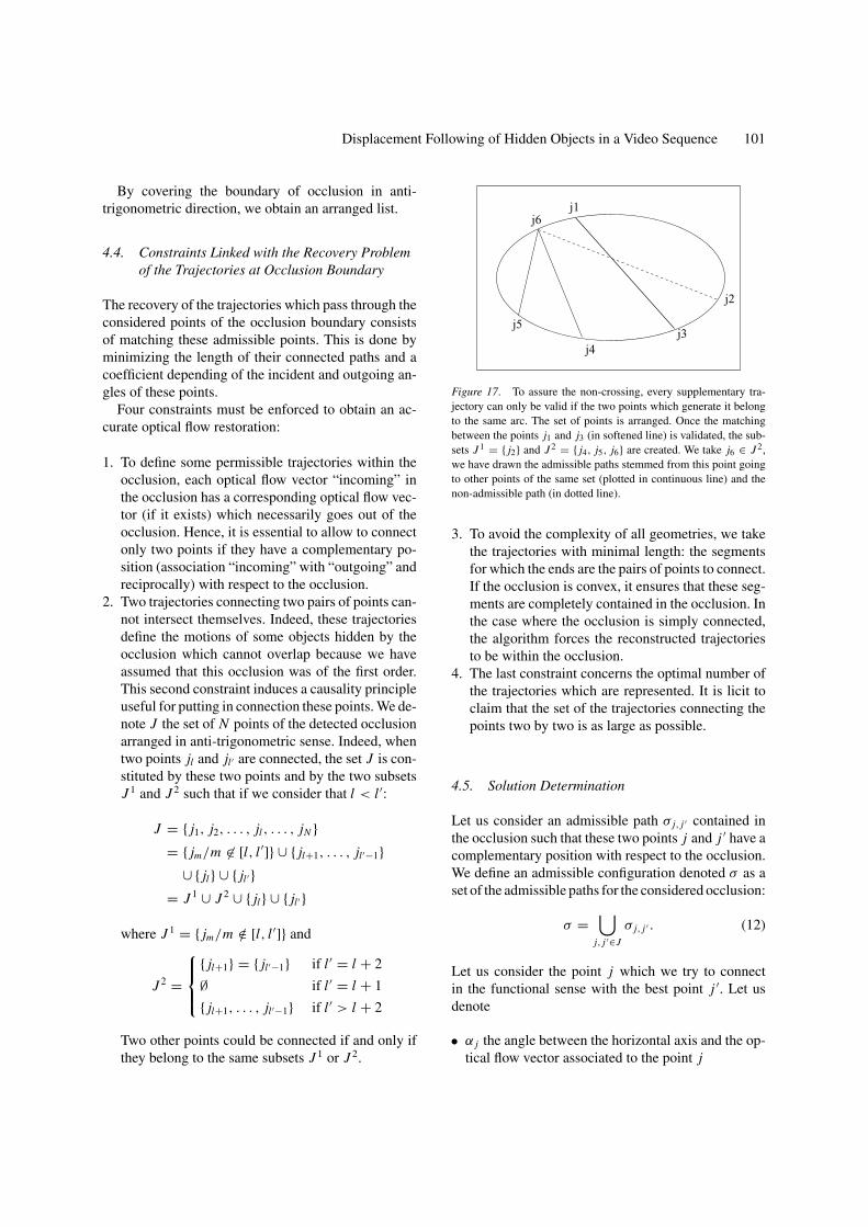
Figure 17. To assure the non-crossing, every supplementary tra-jectory can only be valid if the two points which generate it belongto the same arc. The set of points is arranged. Once the matchingbetween the points j1 and j3 (in softened line) is validated, the sub-sets J 1 = { j2} and J 2 = { j4, j5, j6} are created. We take j6 ∈ J 2,we have drawn the admissible paths stemmed from this point goingto other points of the same set (plotted in continuous line) and thenon-admissible path (in dotted line).

3. To avoid the complexity of all geometries, we takethe trajectories with minimal length: the segmentsfor which the ends are the pairs of points to connect.If the occlusion is convex, it ensures that these seg-ments are completely contained in the occlusion. Inthe case where the occlusion is simply connected,the algorithm forces the reconstructed trajectoriesto be within the occlusion.

4. The last constraint concerns the optimal number ofthe trajectories which are represented. It is licit toclaim that the set of the trajectories connecting thepoints two by two is as large as possible.

4.5. Solution Determination

Let us consider an admissible path σ j, j ′ contained inthe occlusion such that these two points j and j ′ have acomplementary position with respect to the occlusion.We define an admissible configuration denoted σ as aset of the admissible paths for the considered occlusion:

σ =⋃

j, j ′∈J

σ j, j ′ . (12)

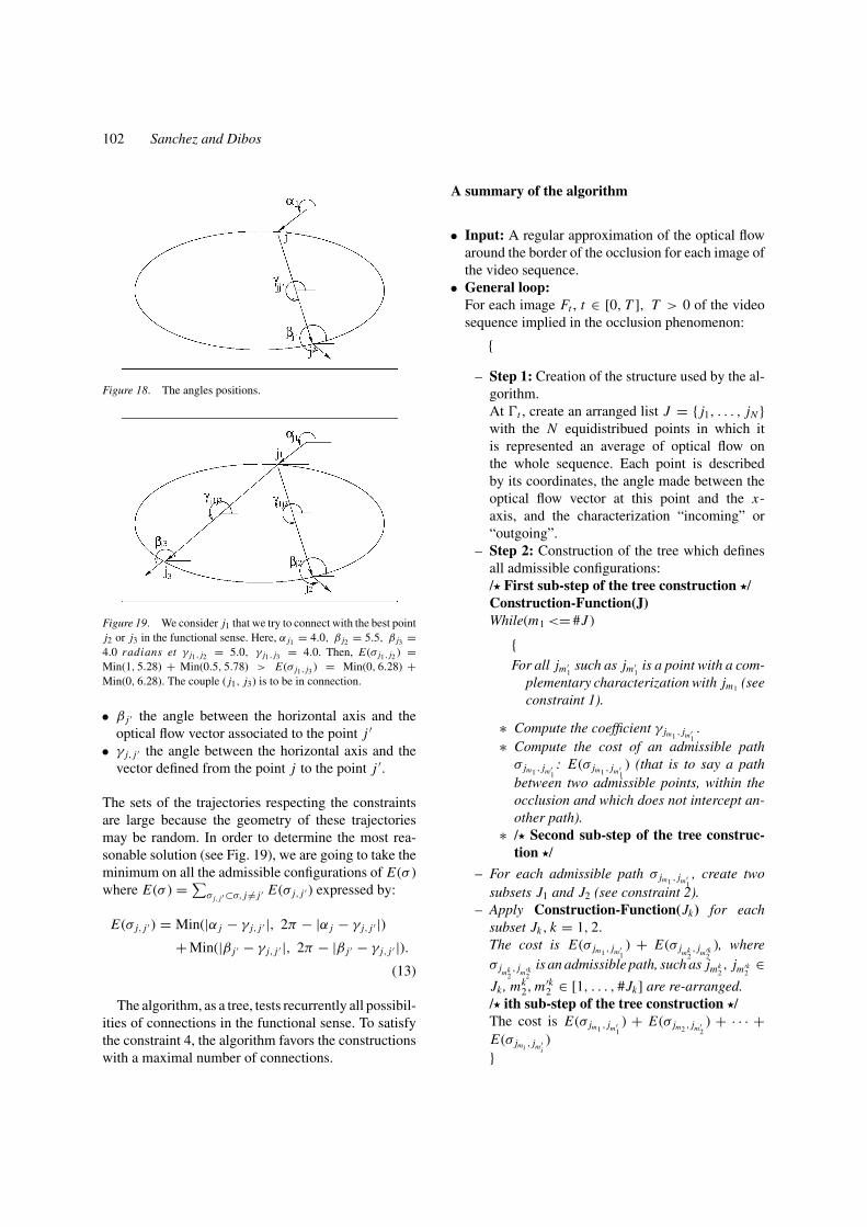
Let us consider the point j which we try to connectin the functional sense with the best point j ′. Let usdenote

• α j the angle between the horizontal axis and the op-tical flow vector associated to the point j


Figure 18. The angles positions.

Figure 19. We consider j1 that we try to connect with the best pointj2 or j3 in the functional sense. Here, α j1 = 4.0, β j2 = 5.5, β j3 =4.0 radians et γ j1, j2 = 5.0, γ j1, j3 = 4.0. Then, E(σ j1, j2 ) =Min(1, 5.28) + Min(0.5, 5.78) > E(σ j1, j3 ) = Min(0, 6.28) +Min(0, 6.28). The couple ( j1, j3) is to be in connection.

• β j ′ the angle between the horizontal axis and theoptical flow vector associated to the point j ′

• γ j, j ′ the angle between the horizontal axis and thevector defined from the point j to the point j ′.

The sets of the trajectories respecting the constraintsare large because the geometry of these trajectoriesmay be random. In order to determine the most rea-sonable solution (see Fig. 19), we are going to take theminimum on all the admissible configurations of E(σ )where E(σ ) = ∑

σ j, j ′ ⊂σ, j = j ′ E(σ j, j ′ ) expressed by:

E(σ j, j ′ ) = Min(|α j − γ j, j ′ |, 2π − |α j − γ j, j ′ |)+ Min(|β j ′ − γ j, j ′ |, 2π − |β j ′ − γ j, j ′ |).

(13)

The algorithm, as a tree, tests recurrently all possibil-ities of connections in the functional sense. To satisfythe constraint 4, the algorithm favors the constructionswith a maximal number of connections.

A summary of the algorithm

• Input: A regular approximation of the optical flowaround the border of the occlusion for each image ofthe video sequence.

• General loop:For each image Ft , t ∈ [0, T ], T > 0 of the videosequence implied in the occlusion phenomenon:

{– Step 1: Creation of the structure used by the al-

gorithm.At �t , create an arranged list J = { j1, . . . , jN }with the N equidistribued points in which itis represented an average of optical flow onthe whole sequence. Each point is describedby its coordinates, the angle made between theoptical flow vector at this point and the x-axis, and the characterization “incoming” or“outgoing”.

– Step 2: Construction of the tree which definesall admissible configurations:/� First sub-step of the tree construction �/Construction-Function(J)While(m1 <= #J )

{For all jm ′

1such as jm ′

1is a point with a com-

plementary characterization with jm1 (seeconstraint 1).

∗ Compute the coefficient γ jm1 , jm′1.

∗ Compute the cost of an admissible pathσ jm1 , jm′

1: E(σ jm1 , jm′

1) (that is to say a path

between two admissible points, within theocclusion and which does not intercept an-other path).

∗ /� Second sub-step of the tree construc-tion �/

– For each admissible path σ jm1 , jm′1, create two

subsets J1 and J2 (see constraint 2).– Apply Construction-Function(Jk) for each

subset Jk, k = 1, 2.

The cost is E(σ jm1 , jm′1) + E(σ jmk

2, jm′k

2), where

σ jmk2, jm′k

2is an admissible path, such as jmk

2, jm ′k

2∈

Jk, mk2, m ′k

2 ∈ [1, . . . , #Jk] are re-arranged./� ith sub-step of the tree construction �/The cost is E(σ jm1 , jm′

1) + E(σ jm2 , jm′

2) + · · · +

E(σ jmi , jm′i)

}


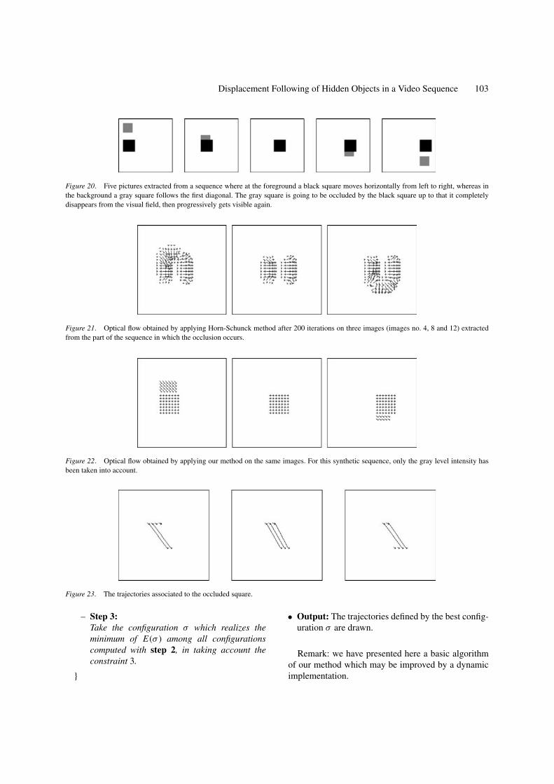
Figure 20. Five pictures extracted from a sequence where at the foreground a black square moves horizontally from left to right, whereas inthe background a gray square follows the first diagonal. The gray square is going to be occluded by the black square up to that it completelydisappears from the visual field, then progressively gets visible again.

Figure 21. Optical flow obtained by applying Horn-Schunck method after 200 iterations on three images (images no. 4, 8 and 12) extractedfrom the part of the sequence in which the occlusion occurs.

Figure 22. Optical flow obtained by applying our method on the same images. For this synthetic sequence, only the gray level intensity hasbeen taken into account.

Figure 23. The trajectories associated to the occluded square.

– Step 3:Take the configuration σ which realizes theminimum of E(σ ) among all configurationscomputed with step 2, in taking account theconstraint 3.

}

• Output: The trajectories defined by the best config-uration σ are drawn.

Remark: we have presented here a basic algorithmof our method which may be improved by a dynamicimplementation.


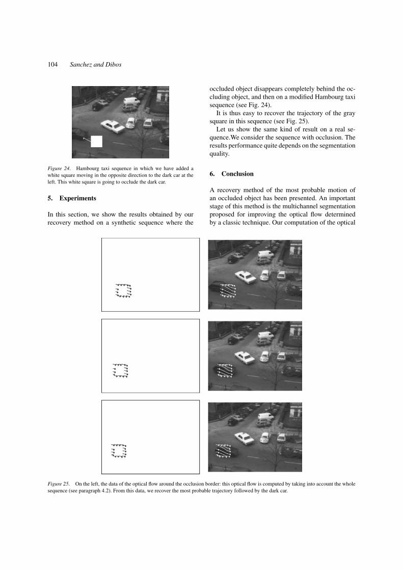
Figure 24. Hambourg taxi sequence in which we have added awhite square moving in the opposite direction to the dark car at theleft. This white square is going to occlude the dark car.

5. Experiments

In this section, we show the results obtained by ourrecovery method on a synthetic sequence where the

Figure 25. On the left, the data of the optical flow around the occlusion border: this optical flow is computed by taking into account the wholesequence (see paragraph 4.2). From this data, we recover the most probable trajectory followed by the dark car.

occluded object disappears completely behind the oc-cluding object, and then on a modified Hambourg taxisequence (see Fig. 24).

It is thus easy to recover the trajectory of the graysquare in this sequence (see Fig. 25).

Let us show the same kind of result on a real se-quence.We consider the sequence with occlusion. Theresults performance quite depends on the segmentationquality.

6. Conclusion

A recovery method of the most probable motion ofan occluded object has been presented. An importantstage of this method is the multichannel segmentationproposed for improving the optical flow determinedby a classic technique. Our computation of the optical


flow and then the experiments on synthetic and real se-quences for recovering the motion of the hidden objectgive satisfying results. From this disocclusion of tra-jectories, the further work consists of realizing a com-plete disocclusion where the occluded object becomesthe occluding object for a sequence when these twoobjects are in motion on a fixed background.

Acknowledgments

We thank very much G. Koepfler (University Paris V)for valuable conversations, and J.F Hochedez (ROB)for the sequences of Sun.

References

Alvarez Leon, L., Escalin Monreal, J., Lefebure, M., and SanchezPerez, J. 1999. A PDE model for computing the optical flow. InProceeding of CEDYA XVI, Universidad de La Palmas de GranCanaria, pp. 1349–1356.

Alvarez Leon, L., Weickert, J., and Sanchez Perez, J. 2000. Reliableestimation of dense optical flow fields with large displacements.International Journal of Computer Vision, 39(1):41–56.

Aubert, G., Kornprobst, P., and Deriche, R. 1999. A mathematicalstudy of regularized optical flow problem in space BV. SIAM.Journal on Mathematical analysis, 30(6):1282–1308.

Ballester, C., Bertalmio, M., Caselles, V., Sapiro, G., Verdera, J.2001. Filling-in by joint interpolation of vectors fields and graylevels. IEEE Trans. Image Processing, 10(8):1200–1211.

Barron, J.L., Fleet, D.J., and Beauchemin, S.S. 1994. Performance ofoptical flow Techniques. International Journal Computer Vision,12(1):43–77.

Bertalmio, M., Sapiro, G., Caselles, V., and Ballester, C. 2000. Im-age inpainting. In Proceeding of SIGGRAPH 2000, New Orleans,USA, pp. 417–424.

Cohen, I. 1993. Nonlinear variational method for optical flow com-putation. In Proc. Eighth Scandinavian Conf. on Image Analysis,Tromso. May 93. Vol. 1, pp. 523–530.

Cohen, I. and Herlin, I. 1999. Non uniform multiresolution methodfor optical flow an phase portrait models: Environment applica-tions. International Journal of Computer Vision, 33(1):29–49.

Deriche, R. and Faugeras, O. 1995. Les EDP en traitement des imageset vision par ordinateur. Rapport INRIA no TR 2697.

Horn, B.K.P. and Schunck, B. 1981. Determining optical flow.Artificial Intelligence, 16(1–3):185–203.

Koepfler, G., Lopez, C., and Rudin, L. 1993. Data fusion by seg-mentation. Application to texture discrimination. 14eme colloqueGRETSI Juan-les-pins, pp. 707–710.

Kumar, A., Tannenbaum, A.R., and Balas, G. 1996 Optical Flow: ACurve Evolution Approach. IEEE transaction on Image Proceed-ing, 5(4):598–610.

Masnou, S. and Morel, J.M. 1998. Level lines based disocclusion. InProceeding IEEE International Conference on Image Processing,Chicago, pp. 254–258.

Morel, J.M. and Solemini, S. 1994. Variational Methods in ImageSegmentation. Birkhauser.

Mumford, D. and Shah, J. 1989. Optimal approximations bypiecewise smooth functions and associated variational problems.Comm. Pure Appl. Math., 42:577–685.

Nesi, P. 1993. Variational approach to optical flow estimation man-aging discontinuities. Image and Vision Computing, 11:419–439.

Orkisz, M. and Clarysse, P. 1996. Estimation du flot optique enpresence de discontinuites: une revue. Traitement du signal, 13(5).

Sanchez, O. 2002. Desoccultation de sequences video: Aspectsmathematique et numerique. PhD thesis. CEREMADE. UniversiteParis 9 Dauphine.

Weickert, J. and Schnorr, C. 2001. Variational optic flow compu-tation with a spatio-temporal smoothness constraint. Journal ofMathematical Imaging and Vision, 14(3):245–255.

Documents

Displacement Following of Hidden Objects in a Video Sequence