Dissecting Saving DynamicsMeasuring Credit, Wealth and Precautionary Effects

Christopher Carroll1 Jiri Slacalek2 Martin Sommer3

1Johns Hopkins University and NBERccarroll@jhu.edu

2European Central Bankjiri.slacalek@ecb.int

3International Monetary Fundmsommer@imf.org

Presentation at Julis-Rabinowitz ConferencePrinceton University, February 2014

US Personal Saving Rate (s), 1966–2011

1970 1975 1980 1985 1990 1995 2000 2005 20100

2

4

6

8

10

12

14

Perc

ent o

f Dis

posa

ble

Inco

me

Literature

I “Wealth Effects”I Modigliani, Klein, MPS model, ...

I st = −0.05mt + other stuff

I “Precautionary”I Carroll (1992)

I Saving rate rises in recessionsI ∆ logCt+1 strongly related to Et(ut+1 − ut)

I “Credit Availability”I Secular Trend:

I Parker (2000), Dynan and Kohn (2007), Muellbauer (manypapers)

I Cyclical Dynamics:I Guerrieri and Lorenzoni (2011), Eggertsson and Krugman

(2011), Hall (2011)

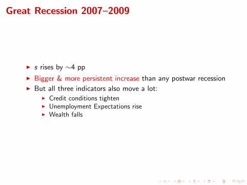
Great Recession 2007–2009

I s rises by ∼4 pp

I Bigger & more persistent increase than any postwar recessionI But all three indicators also move a lot:

I Credit conditions tightenI Unemployment Expectations riseI Wealth falls

Personal Saving Rate 2007– ↑

−4−2

02

4D

evia

tion

from

Sta

rt−of

−Rec

essi

on V

alue

in %

0 2 4 6 8 10 12 14 16 18 20Quarters after Start of Recession

Historical Range Historical Mean 2007−2011

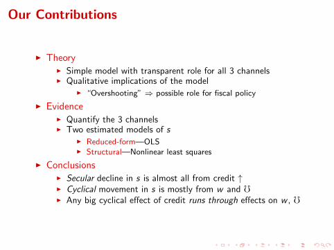
Our Contributions

I TheoryI Simple model with transparent role for all 3 channelsI Qualitative implications of the model

I “Overshooting” ⇒ possible role for fiscal policy

I EvidenceI Quantify the 3 channelsI Two estimated models of s

I Reduced-form—OLSI Structural—Nonlinear least squares

I ConclusionsI Secular decline in s is almost all from credit ↑I Cyclical movement in s is mostly from w and fI Any big cyclical effect of credit runs through effects on w , f

Theory a la Carroll and Toche (2009)

I CRRA utility, labor supply `, agg wage W, emp status ξ:

v(mmmt) = maxccct

u(ccct) + βEt

[v(mmmt+1)

]s.t.

mmmt+1 = (mmmt − ccct)R + `t+1Wt+1ξt+1

I ξt+1 ∈ {ξu, ξe} where ξu < ξe

I ` and W grow at constant rateI Tractability: unemployment shocks are permanent

I If ξt = ξu then ξt+1 = ξu

I Target wealth m exists and is stable:I Consumption chosen so that mt → m

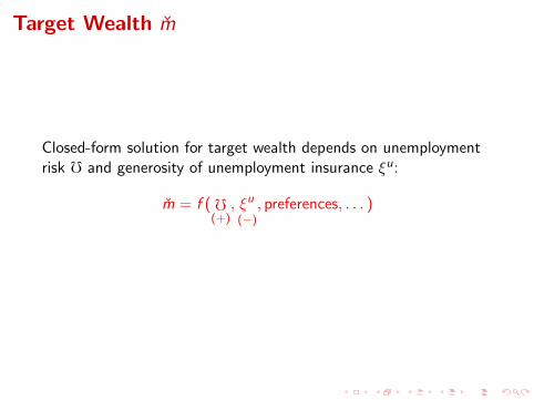
Target Wealth m

Closed-form solution for target wealth depends on unemploymentrisk f and generosity of unemployment insurance ξu:

m = f ( f(+), ξu

(−), preferences, . . . )

Consumption After a Wealth Shock

Dmt+1e = 0 �

cHmL�

ct � � ct+1

Wealth Shock

� Target

cHmL�

mÇ

mt

m

cÇ

c

Permanent Rise in f

Sustainable c �

� cHmL after unemployment rate increase

� Target

cHmL�

mÇ m

c

Saving Rate After a Permanent Rise in f

� Overshooting

tTime

sÇ

t'

st

Credit Easing/Financial Innovation & Deregulation

� Orig Target� D mt+1

e = 0� Orig cHmL

New cHmL �

-h 0.m

c

m is close to linear in credit conditions

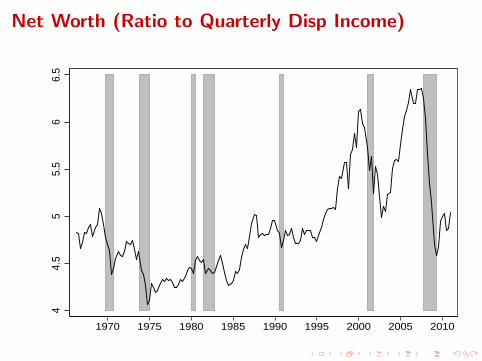
Net Worth (Ratio to Quarterly Disp Income)

44.

55

5.5

66.

5

1970 1975 1980 1985 1990 1995 2000 2005 2010

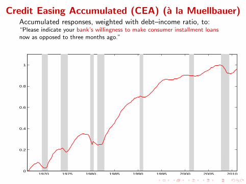
Credit Easing Accumulated (CEA) (a la Muellbauer)Accumulated responses, weighted with debt–income ratio, to:“Please indicate your bank’s willingness to make consumer installment loansnow as opposed to three months ago.”

1970 1975 1980 1985 1990 1995 2000 2005 20100

0.2

0.4

0.6

0.8

1

ft Implied by Michigan U ExpectationsI Regress: ∆4ut+4 = α0 + α1UExptI U risk: ft = ut + ∆4ut+4

I ∆4ut+4 ≡ ut+4 − ut , ∆4ut+4 ≡ fitted valuesI ft tracks but precedes actual U

UExp: “How about people out of work during the coming 12 months—do you think

that there will be more unemployment than now, about the same, or less?”

24

68

10

1970 1975 1980 1985 1990 1995 2000 2005 2010

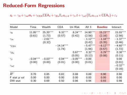
Reduced-Form Regressions

st = γ0 +γmmt +γCEACEAt +γEuEtut+4 +γt t +γuC (Etut+4×CEAt)+εt

Model Time Wealth CEA Un Risk All 3 Baseline Interact

γ0 11.95∗∗∗ 25.20∗∗∗ 9.32∗∗∗ 8.24∗∗∗ 14.90∗∗∗ 15.23∗∗∗ 15.55∗∗∗

(0.61) (1.73) (0.57) (0.42) (2.56) (2.16) (2.56)γm −2.61∗∗∗ −1.12∗∗∗ −1.18∗∗∗ −1.37∗∗∗

(0.32) (0.42) (0.35) (0.46)γCEA −14.14∗∗∗ −5.47∗∗∗ −6.12∗∗∗ −4.60∗∗∗

(1.74) (1.94) (0.57) (1.72)γEu 0.67∗∗∗ 0.32∗∗∗ 0.29∗∗∗ 0.38∗∗∗

(0.05) (0.12) (0.08) (0.11)γt −0.04∗∗∗ −0.03∗∗∗ 0.04∗∗∗ −0.05∗∗∗ −0.00 0.00

(0.00) (0.00) (0.01) (0.00) (0.01) (0.01)γuC −0.32∗∗

(0.16)

R2 0.70 0.85 0.82 0.88 0.89 0.90 0.90F stat p val 0.00 0.00 0.00 0.00 0.00 0.00 0.00DW stat 0.30 0.69 0.50 0.86 0.94 0.93 0.98

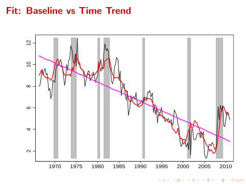
Fit: Baseline vs Time Trend

24

68

1012

1970 1975 1980 1985 1990 1995 2000 2005 2010

st = γ1 + γmmt + γCEACEAt + γEuEtut+4 + γ′Xt + εt

Model Baseline Uncert st−1 Debt Full Controls Post-80 IV

γm −1.18∗∗∗ −1.21∗∗∗−0.31 −0.80∗∗ −1.30∗∗∗ −1.50 −2.02∗∗∗

(0.35) (0.36) (0.22) (0.36) (0.31) (1.25) (0.49)γCEA −6.12∗∗∗ −5.97∗∗∗−2.87∗∗∗−5.40∗∗∗ −6.24∗∗∗ −5.00∗∗ −5.85∗∗∗

(0.57) (0.65) (0.53) (0.73) (0.63) (2.00) (1.17)γEu 0.29∗∗∗ 0.28∗∗∗ 0.14∗∗∗ 0.34∗∗∗ 0.12 0.30∗∗ 0.08

(0.08) (0.09) (0.05) (0.07) (0.09) (0.14) (0.13)γσ 0.26

(0.47)γs 0.57∗∗∗

(0.07)γd −1.91

(1.16)γr 0.13∗∗∗

(0.04)γGS −0.12

(0.08)γCS −0.31∗∗

(0.14)γ0post80 −1.48

(7.90)γmpost80 0.56

(1.29)γCEApost80 −2.35

(2.13)

Fit: Baseline vs Post-1980

24

68

1012

1970 1975 1980 1985 1990 1995 2000 2005 2010

Fit: Baseline vs Full Controls

24

68

1012

1970 1975 1980 1985 1990 1995 2000 2005 2010

Structural Estimation—Nonlinear Least Squares

Minimize distance between model-implied stheort and actual smeas

t :

Θ = arg minT∑t=1

(smeast −stheor

t

(Θ;mt−m

(m(CEAt),f(Etut+4)

)))2

,

where

I Θ = {β, θm, θCEA, θf, θu}I mt = θm + θCEACEAt

I ft = θf + θuEtut+4

I β: discount factor

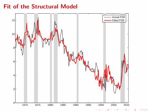
Fit of the Structural Model

1970 1975 1980 1985 1990 1995 2000 2005 20100

2

4

6

8

10

12Actual PSRFitted PSR

Decomposition of Fitted PSRFix ft and CEAt at their sample means, back out the implied st

1970 1975 1980 1985 1990 1995 2000 2005 20100

2

4

6

8

10

12

Fitted PSRFitted PSR excl. UncertaintyFitted PSR excl. Uncertainty and CEA

Fit: Structural Model vs Reduced-Form

24

68

1012

1970 1975 1980 1985 1990 1995 2000 2005 2010

Actual Reduced−Form Structural

PSR Forecasts—In Sample

Great Recession 2007–2010

Variable Reduced-Form Model Structural Model Actual ∆st

γm ×∆mt −1.18×−1.39 = 1.64 −0.97×−1.39 = 1.34γCEA ×∆CEAt −6.12×−0.11 = 0.64 −6.38×−0.11 = 0.67γEu ×∆Etut+4 0.29× 4.33 = 1.24 0.32× 4.33 = 1.39

Explained ∆st 3.53 3.40 2.93

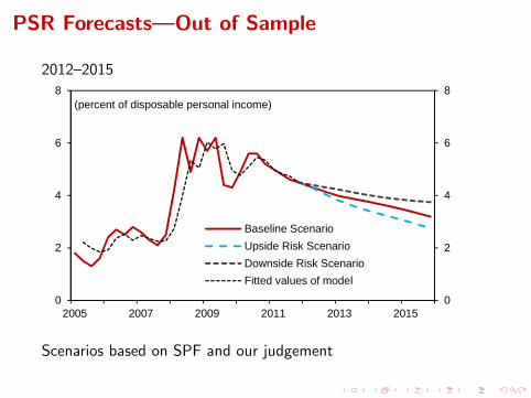
PSR Forecasts—Out of Sample

2012–2015

0

2

4

6

8

0

2

4

6

8

2005 2007 2009 2011 2013 2015

Baseline Scenario

Upside Risk Scenario

Downside Risk Scenario

Fitted values of model

(percent of disposable personal income)

Scenarios based on SPF and our judgement

Conclusions

I All three effects present

I Easier borrowing largely explains secular decline sI Order of importance in Great Recession:

1. Wealth shock2. Labor income risk3. Credit tightening

I ⇒ if credit has big cyclical effect, comes thru w and f

References

Carroll, Christopher D. (1992): “The Buffer-Stock Theory of Saving: Some Macroeconomic Evidence,”Brookings Papers on Economic Activity, 1992(2), 61–156,http://econ.jhu.edu/people/ccarroll/BufferStockBPEA.pdf.

Carroll, Christopher D., and Patrick Toche (2009): “A Tractable Model of Buffer Stock Saving,” NBERWorking Paper Number 15265, http://econ.jhu.edu/people/ccarroll/papers/ctDiscrete.

Dynan, Karen E., and Donald L. Kohn (2007): “The Rise in US Household Indebtedness: Causes andConsequences,” in The Structure and Resilience of the Financial System, ed. by Christopher Kent, and JeremyLawson, pp. 84–113. Reserve Bank of Australia.

Eggertsson, Gauti B., and Paul Krugman (2011): “Debt, Deleveraging, and the Liquidity Trap: AFisher-Minsky-Koo Approach,” Manuscript, NBER Summer Institute.

Guerrieri, Veronica, and Guido Lorenzoni (2011): “Credit Crises, Precautionary Savings and the LiquidityTrap,” Manuscript, MIT Department of Economics.

Hall, Robert E. (2011): “The Long Slump,” AEA Presidential Address, ASSA Meetings, Denver.

Parker, Jonathan A. (2000): “Spendthrift in America? On Two Decades of Decline in the U.S. Saving Rate,”in NBER Macroeconomics Annual 1999, ed. by Ben S. Bernanke, and Julio J. Rotemberg, vol. 14, pp.317–387. NBER.

Background Slides

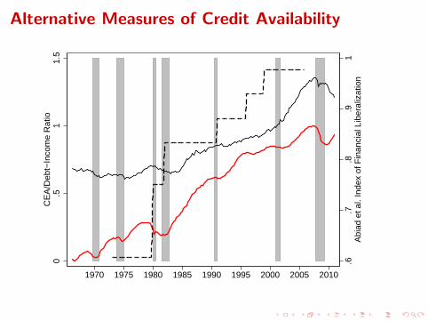
Alternative Measures of Credit Availability

.6.7

.8.9

1A

biad

et a

l. In

dex

of F

inan

cial

Lib

eral

izat

ion

0.5

11.

5C

EA

/Deb

t−In

com

e R

atio

1970 1975 1980 1985 1990 1995 2000 2005 2010

Assumptions/Scenarios for Out-of-Sample Forecasts

Sources: Haver Analytics and authors' estimates.

400

450

500

550

600

650

700

400

450

500

550

600

650

700

2005 2007 2009 2011 2013 2015

Baseline scenario

Upside risk scenario

Downside risk scenario

(percent of disposable personal income)

4

6

8

10

12

4

6

8

10

12

2005 2007 2009 2011 2013 2015

Baseline scenario

Upside risk scenario

Downside riskscenarioUnemploymentexpectations

(percent of labor force)

0.7

0.8

0.9

1.0

1.1

1.2

1.3

0.7

0.8

0.9

1.0

1.1

1.2

1.3

2005 2007 2009 2011 2013 2015

Baseline scenario

Upside risk scenario

Downside risk scenario

0

2

4

6

8

0

2

4

6

8

2005 2007 2009 2011 2013 2015

Baseline Scenario

Upside Risk ScenarioDownside Risk Scenario

Fitted values of model

(percent of disposable personal income)

Household net wealth Unemployment rate

Credit conditions Household saving rate

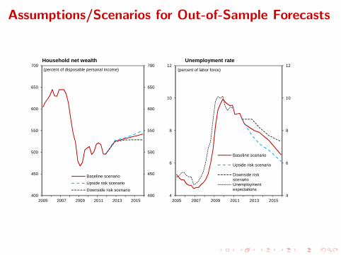
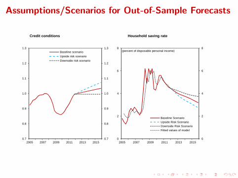
Assumptions/Scenarios for Out-of-Sample Forecasts

Sources: Haver Analytics and authors' estimates.

400

450

500

550

600

650

700

400

450

500

550

600

650

700

2005 2007 2009 2011 2013 2015

Baseline scenario

Upside risk scenario

Downside risk scenario

(percent of disposable personal income)

4

6

8

10

12

4

6

8

10

12

2005 2007 2009 2011 2013 2015

Baseline scenario

Upside risk scenario

Downside riskscenarioUnemploymentexpectations

(percent of labor force)

0.7

0.8

0.9

1.0

1.1

1.2

1.3

0.7

0.8

0.9

1.0

1.1

1.2

1.3

2005 2007 2009 2011 2013 2015

Baseline scenario

Upside risk scenario

Downside risk scenario

0

2

4

6

8

0

2

4

6

8

2005 2007 2009 2011 2013 2015

Baseline Scenario

Upside Risk ScenarioDownside Risk Scenario

Fitted values of model

(percent of disposable personal income)

Household net wealth Unemployment rate

Credit conditions Household saving rate

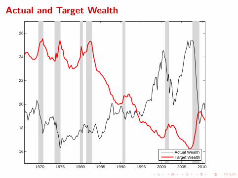
Actual and Target Wealth

1970 1975 1980 1985 1990 1995 2000 2005 2010

16

18

20

22

24

26

Actual WealthTarget Wealth

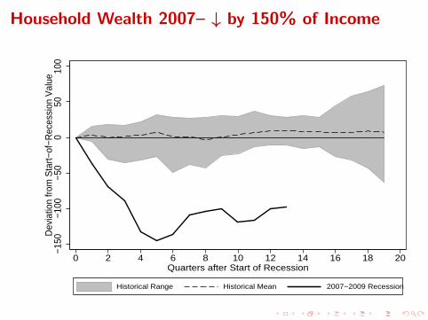
Household Wealth 2007– ↓ by 150% of Income

−150

−100

−50

050

100

Dev

iatio

n fro

m S

tart−

of−R

eces

sion

Val

ue

0 2 4 6 8 10 12 14 16 18 20Quarters after Start of Recession

Historical Range Historical Mean 2007−2009 Recession

Sustained Expectations of Rising Unemp RiskThomson Reuters/University of Michigan Et(ut+4 − ut)

1970 1975 1980 1985 1990 1995 2000 2005 2010

30

40

50

60

70

80

90

100

110

120

130

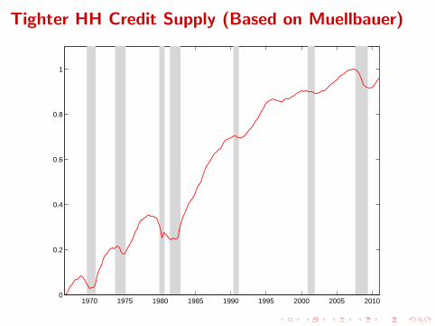
Tighter HH Credit Supply (Based on Muellbauer)

1970 1975 1980 1985 1990 1995 2000 2005 20100

0.2

0.4

0.6

0.8

1

Consumption Function

Dct+1e =0 �

Dmt+1e = 0 �

ceHmL=Stable Arm �

Steady State �

mte

cte

Overshooting and Fiscal Policy

DSGE models:

I Frictions, frictions everywhere; but missing hereI If ∆c imposes ‘external’ costs

I Sticky prices/wagesI Capital (or Investment) adjustment costsI Other reasons for ‘pecuniary externalities’

I ⇒ ‘stimulus’ payments, fiscal policy may reduce cost of cycle

I Justification for ‘automatic stabilizers’?

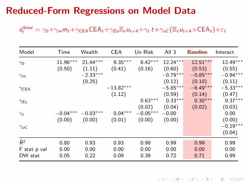
Reduced-Form Regressions on Model Data

stheort = γ0+γmmt+γCEACEAt+γEuEtut+4+γt t+γuC (Etut+4×CEAt)+εt

Model Time Wealth CEA Un Risk All 3 Baseline Interact

γ0 11.96∗∗∗ 21.44∗∗∗ 9.35∗∗∗ 8.42∗∗∗ 12.24∗∗∗ 12.51∗∗∗ 12.49∗∗∗

(0.50) (1.11) (0.41) (0.16) (0.60) (0.53) (0.55)γm −2.33∗∗∗ −0.79∗∗∗ −0.85∗∗∗ −0.94∗∗∗

(0.25) (0.12) (0.10) (0.11)γCEA −13.82∗∗∗ −5.85∗∗∗ −6.49∗∗∗ −5.33∗∗∗

(1.12) (0.59) (0.14) (0.47)γEu 0.63∗∗∗ 0.33∗∗∗ 0.30∗∗∗ 0.37∗∗∗

(0.02) (0.04) (0.02) (0.03)γt −0.04∗∗∗ −0.03∗∗∗ 0.04∗∗∗ −0.05∗∗∗ −0.00 0.00

(0.00) (0.00) (0.01) (0.00) (0.00) (0.00)γuC −0.19∗∗∗

(0.04)

R2 0.80 0.93 0.93 0.98 0.99 0.99 0.99F stat p val 0.00 0.00 0.00 0.00 0.00 0.00 0.00DW stat 0.05 0.22 0.09 0.39 0.72 0.71 0.99

Reduced-Form Regressions on Actual Data

smeast = γ0+γmmt+γCEACEAt+γEuEtut+4+γt t+γuC (Etut+4×CEAt)+εt

Model Time Wealth CEA Un Risk All 3 Baseline Interact

γ0 11.95∗∗∗ 25.20∗∗∗ 9.32∗∗∗ 8.24∗∗∗ 14.90∗∗∗ 15.23∗∗∗ 15.55∗∗∗

(0.61) (1.73) (0.57) (0.42) (2.56) (2.16) (2.56)γm −2.61∗∗∗ −1.12∗∗∗ −1.18∗∗∗ −1.37∗∗∗

(0.32) (0.42) (0.35) (0.46)γCEA −14.14∗∗∗ −5.47∗∗∗ −6.12∗∗∗ −4.60∗∗∗

(1.74) (1.94) (0.57) (1.72)γEu 0.67∗∗∗ 0.32∗∗∗ 0.29∗∗∗ 0.38∗∗∗

(0.05) (0.12) (0.08) (0.11)γt −0.04∗∗∗ −0.03∗∗∗ 0.04∗∗∗ −0.05∗∗∗ −0.00 0.00

(0.00) (0.00) (0.01) (0.00) (0.01) (0.01)γuC −0.32∗∗

(0.16)

R2 0.70 0.85 0.82 0.88 0.89 0.90 0.90F stat p val 0.00 0.00 0.00 0.00 0.00 0.00 0.00DW stat 0.30 0.69 0.50 0.86 0.94 0.93 0.98