Embed Size (px)
Citation preview

dissertation
i
THE FLORIDA STATE UNIVERSITY
COLLEGE OF ARTS AND SCIENCES
VARIATIONAL DATA ASSIMILATION WITH 2-D SHALLOW
WATER EQUATIONS AND 3-D FSU GLOBAL SPECTRAL MODELS
By
A Dissertation submitted to theDepartment of Mathematicsin partial fulfillment of the
requirements for the degree ofDoctor of Philosophy
Degree Awarded:Fall Semester, 1993
Copyright 1993Zhi Wang
All Rights Reserved
Copyright c© 1993
Copyright 1993Zhi Wang
All Rights ReservedZHI WANG
All Rights Reserved
The members of the Committee approve the dissertation of ZHI WANG defended
on November 10, 1993.
I. Michael Navon
Professor Directing Thesis
James J. O’Brien
Outside Committee Member
Christopher Hunter
Committee Member
Francois Xavier Le Dimet
Committee Member
Louis N. Howard
Committee Member

This work is dedicated to My Wife, My Parents, My Brothers and
Sister.
iii
ACKNOWLEDGEMENTS
First, and foremost, I would like to express my thanks to Dr. I. M. Navon, my
major professor. He was the driving force behind the development of this study. I
am fortunate and thankful to have had Dr. I. M. Navon always there to consistently
point me in the right direction. I also wish to thank Dr. James J. O’Brien, Dr. C.
Hunter, Dr. F. X. Le Dimet and Dr. L. Howard for serving on my committee.
The author thanks Dr. F. X. Le Dimet for contributing original ideas related
to the second order adjoint analysis and optimal nudging assimilation. His help is
highly appreciated.
Special thanks go to T. N. Krishnamurti at the Department of Meteorology of the
Florida State University for providing me the Florida State University Global Spec-
tral Model (FSUGSM), to the many people at the Department of Mathematics and
to Dr. X. Zou of the Supercomputer Computations Research Institute of the Florida
State University for her contribution towards my understanding of the subject.
My deepest appreciation to all my friends who gave me encouragement through
the last few years.
The author gratefully acknowledges the support of Dr. Pamela Stephens, Direc-
tor of GARP Division of the Atmospheric Sciences at NSF. This research was funded
by NSF Grant ATM-9102851. Additional support was provided by the Supercom-
iv

puter Computations Research Institute at Florida State University, which is partially
funded by the Department of Energy through contract No. DE-FC0583ER250000.
v
TABLE OF CONTENTS
List of Tables x
List of Figures xi
Abstract xiv
1 INTRODUCTION 1
1.1 Overview . . . . . . . . . . . . . . . . . . . . . . . . . . . . . . . . . . 1
1.2 Four dimensional variational data assimilation in meteorology . . . . 5
1.3 Preliminaries . . . . . . . . . . . . . . . . . . . . . . . . . . . . . . . 8
1.3.1 The definition of a variational method . . . . . . . . . . . . . 8
1.3.2 Description of the first order adjoint analysis . . . . . . . . . 12
1.4 The theme of my dissertation . . . . . . . . . . . . . . . . . . . . . . 16
2 SECOND ORDER ADJOINT ANALYSIS: THEORY AND AP-
PLICATIONS 21
2.1 Introduction . . . . . . . . . . . . . . . . . . . . . . . . . . . . . . . . 21
2.2 The second order adjoint model . . . . . . . . . . . . . . . . . . . . . 22
2.2.1 Theory of the second order adjoint model . . . . . . . . . . . . 22
2.2.2 The estimate of the condition number of the Hessian . . . . . 25
2.3 The derivation of the second order adjoint model for the shallow water
equations model . . . . . . . . . . . . . . . . . . . . . . . . . . . . . . 27
2.3.1 The verification of the correctness of the first and the second
order adjoint models . . . . . . . . . . . . . . . . . . . . . . . 31
vi

2.4 Second order adjoint information . . . . . . . . . . . . . . . . . . . . 32
2.4.1 Calculation of the Hessian/vector product . . . . . . . . . . . 32
2.4.2 The uniqueness of the solution . . . . . . . . . . . . . . . . . . 33
2.4.3 Convergence analysis . . . . . . . . . . . . . . . . . . . . . . . 35
2.5 Sensitivity analysis for observations . . . . . . . . . . . . . . . . . . . 37
2.5.1 Sensitivity theory for observation . . . . . . . . . . . . . . . . 37
2.5.2 Numerical results from model generated data . . . . . . . . . 40
2.5.3 Numerical results using real analysis of First Global Geophys-
ical Experiment (FGGE) data . . . . . . . . . . . . . . . . . . 42
2.6 Conclusions . . . . . . . . . . . . . . . . . . . . . . . . . . . . . . . . 44
3 THE ADJOINT TRUNCATED NEWTON ALGORITHM FOR
LARGE-SCALE UNCONSTRAINED OPTIMIZATION 58
3.1 Introduction . . . . . . . . . . . . . . . . . . . . . . . . . . . . . . . . 58
3.2 The adjoint Newton algorithm . . . . . . . . . . . . . . . . . . . . . . 60
3.2.1 Description of the first and second order adjoint theories . . . 60
3.2.2 The adjoint truncated-Newton method. . . . . . . . . . . . . . 62
3.3 Numerical results obtained using the adjoint truncated-Newton algo-
rithm. . . . . . . . . . . . . . . . . . . . . . . . . . . . . . . . . . . . 63
3.3.1 Application of the adjoint truncated-Newton algorithm to vari-
ational data assimilation . . . . . . . . . . . . . . . . . . . . . 64
3.3.2 Numerical results . . . . . . . . . . . . . . . . . . . . . . . . . 65
3.3.3 An accuracy analysis of the Hessian/vector product. . . . . . . 67
3.4 Conclusions . . . . . . . . . . . . . . . . . . . . . . . . . . . . . . . . 72
4 THE FSU GLOBAL SPECTRAL MODEL 79
4.1 Introduction . . . . . . . . . . . . . . . . . . . . . . . . . . . . . . . . 79
4.2 Model equations . . . . . . . . . . . . . . . . . . . . . . . . . . . . . . 82
vii
4.3 Spectral form of the governing equations . . . . . . . . . . . . . . . . 87
4.3.1 Grid to spectral transform . . . . . . . . . . . . . . . . . . . . 89
4.3.2 Spectral to grid transform . . . . . . . . . . . . . . . . . . . . 91
4.4 The semi-implicit algorithm . . . . . . . . . . . . . . . . . . . . . . . 91
4.5 Vertical discretization . . . . . . . . . . . . . . . . . . . . . . . . . . . 94
5 4-D VARIATIONAL DATA ASSIMILATION WITH THE FSU
GLOBAL SPECTRAL MODEL 101
5.1 Introduction . . . . . . . . . . . . . . . . . . . . . . . . . . . . . . . . 101
5.2 Model developments and numerical validation . . . . . . . . . . . . . 102
5.2.1 The cost function and its gradient with respect to control vari-
ables . . . . . . . . . . . . . . . . . . . . . . . . . . . . . . . . 102
5.2.2 The accuracy of the tangent linear model . . . . . . . . . . . . 104
5.2.3 The accuracy of the first order adjoint model . . . . . . . . . . 105
5.3 Descent algorithms and scaling . . . . . . . . . . . . . . . . . . . . . 108
5.3.1 The LBFGS algorithm of Liu and Nocedal . . . . . . . . . . . 108
5.3.2 Weighting and scaling . . . . . . . . . . . . . . . . . . . . . . 109
5.4 Numerical results of the variational data assimilation . . . . . . . . . 111
5.4.1 Numerical results with shifted initial conditions . . . . . . . . 112
5.4.2 Numerical results with randomly perturbed initial conditions . 114
5.4.3 Impact of horizontal diffusion . . . . . . . . . . . . . . . . . . 115
5.4.4 Impact of observations distributed in time . . . . . . . . . . . 117
5.5 Conclusions . . . . . . . . . . . . . . . . . . . . . . . . . . . . . . . . 118
6 VARIATIONAL NUDGING DATA ASSIMILATION 134
6.1 Introduction . . . . . . . . . . . . . . . . . . . . . . . . . . . . . . . . 134
6.2 Nudging data assimilation . . . . . . . . . . . . . . . . . . . . . . . . 137
6.2.1 Some simple examples . . . . . . . . . . . . . . . . . . . . . . 137
viii
6.2.2 The basic theory of nudging data assimilation . . . . . . . . . 140
6.2.3 Variational nudging data assimilation . . . . . . . . . . . . . . 142
6.2.4 Identifiability and stability of parameter estimation . . . . . . 145
6.3 Numerical results of the variational data assimilation . . . . . . . . . 148
6.3.1 Variational nudging data assimilation with the adiabatic ver-
sion of the FSU global spectral model . . . . . . . . . . . . . . 149
6.3.2 Variational nudging data assimilation with the FSU global
spectral model in its full-physics operational form . . . . . . . 153
6.3.3 Comparisons of estimated nudging, optimal nudging and vari-
ational data assimilation . . . . . . . . . . . . . . . . . . . . . 155
6.4 Conclusions . . . . . . . . . . . . . . . . . . . . . . . . . . . . . . . . 156
7 SUMMARY AND CONCLUSIONS 172
A A simple example with exact solutions 178
B A nonlinear model with exact solutions. 182
C TN: Nash’s Truncated Newton Method. 187
D The continuous form of the adjoint equations 192
E Kalman filtering, variational data assimilation and variational nudg-
ing data assimilation 194
F Physical processes 199
F.0.1 Radiative processes . . . . . . . . . . . . . . . . . . . . . . . . 199
F.0.2 Cumulus convection and large scale condensation . . . . . . . 201
F.0.3 Boundary layer processes . . . . . . . . . . . . . . . . . . . . . 204
F.0.4 Dry convective adjustment . . . . . . . . . . . . . . . . . . . . 207
ix
F.0.5 Surface topography . . . . . . . . . . . . . . . . . . . . . . . . 208
F.0.6 Computational requirements . . . . . . . . . . . . . . . . . . . 208
REFERENCES 209
x
LIST OF TABLES
2.1 A comparison between the actual and predicted changes due to iden-
tical perturbations at specified locations at the beginning of the as-
similation window. . . . . . . . . . . . . . . . . . . . . . . . . . . . . 57
3.1 Numerical results of minimization algorithms: adjoint truncated New-
ton, truncated Newton and LBFGS for the minimization of the cost
function in the variational data assimilation problem when observa-
tions are model generated and control variables are the initial conditions. 76
3.2 Rms errors between the Hessian/vector products obtained by using
the second order adjoint and the finite-difference techniques for vari-
ous differencing parameters at the end of 15 iterations of the adjoint
truncated Newton minimization algorithm, respectively. The maxi-
mum number of conjugate gradient inner-iterations is 4 and h is the
differencing parameter used in the original truncated Newton algo-
rithm of Nash minimization algorithm. . . . . . . . . . . . . . . . . . 77
4.1 Gaussian latitudes of the T-42 model. + indicates north, and − south. 92
5.1 Rms errors of temperature . . . . . . . . . . . . . . . . . . . . . . . . 126
6.1 Optimal nudging coefficients obtained by VNDA where the . . . . . . 158
B.1 Errors between the true evolution given by . . . . . . . . . . . . . . . 185
B.2 The absolute errors between the exact and approximate obtained by
second order adjoint integration Hessian/vector product. . . . . . . . 186
xi
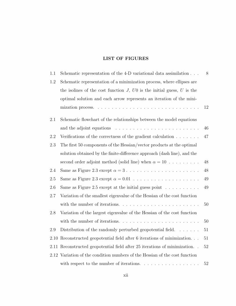
LIST OF FIGURES
1.1 Schematic representation of the 4-D variational data assimilation . . . 8
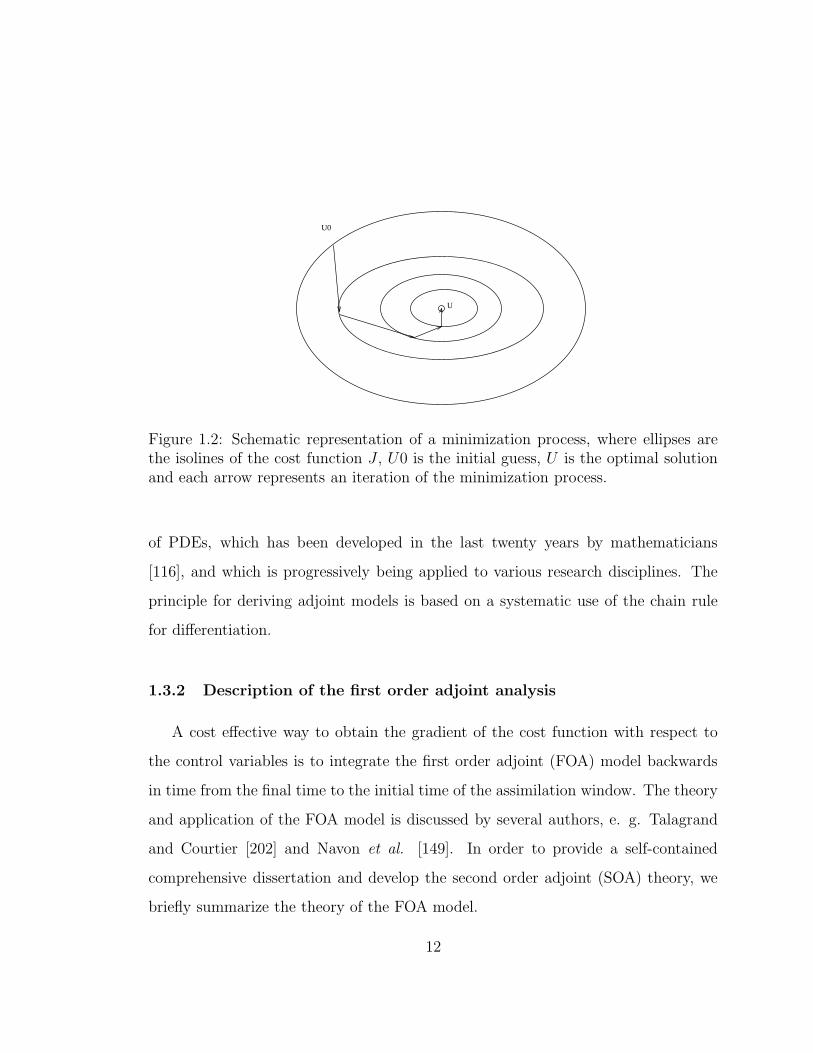
1.2 Schematic representation of a minimization process, where ellipses are
the isolines of the cost function J , U0 is the initial guess, U is the
optimal solution and each arrow represents an iteration of the mini-
mization process. . . . . . . . . . . . . . . . . . . . . . . . . . . . . . 12
2.1 Schematic flowchart of the relationships between the model equations
and the adjoint equations . . . . . . . . . . . . . . . . . . . . . . . . 46
2.2 Verifications of the correctness of the gradient calculation . . . . . . . 47
2.3 The first 50 components of the Hessian/vector products at the optimal
solution obtained by the finite-difference approach (dash line), and the
second order adjoint method (solid line) when α = 10 . . . . . . . . . 48
2.4 Same as Figure 2.3 except α = 3 . . . . . . . . . . . . . . . . . . . . . 48
2.5 Same as Figure 2.3 except α = 0.01 . . . . . . . . . . . . . . . . . . . 49
2.6 Same as Figure 2.5 except at the initial guess point . . . . . . . . . . 49
2.7 Variation of the smallest eigenvalue of the Hessian of the cost function
with the number of iterations. . . . . . . . . . . . . . . . . . . . . . . 50
2.8 Variation of the largest eigenvalue of the Hessian of the cost function
with the number of iterations. . . . . . . . . . . . . . . . . . . . . . . 50
2.9 Distribution of the randomly perturbed geopotential field. . . . . . . 51
2.10 Reconstructed geopotential field after 6 iterations of minimization. . . 51
2.11 Reconstructed geopotential field after 25 iterations of minimization. . 52
2.12 Variation of the condition numbers of the Hessian of the cost function
with respect to the number of iterations. . . . . . . . . . . . . . . . . 52
xii
2.13 Time variation of the sensitivities of cost function J . . . . . . . . . . 53
2.14 Time variation of the sensitivities of cost function J to 1% observa-
tional error at points (x10, y10) (solid line) (x5, y15) (dotted line), and
(x15, y5) (dash line) in the wind and the geopotential fields. . . . . . . 54
2.15 Time variation of the sensitivities of cost function J to 1% observa-
tional error on all grid points in the wind and the geopotential fields. 54
2.16 Distribution of (a) the geopotential and (b) the wind fields for the First
Global Geophysical Experiment (FGGE) data at 0UTC 05/26, 1979
on the 500mb. The contour intervals are 200m2/s2 and the magnitude
of maximum vector is 0.311E+02m/s. . . . . . . . . . . . . . . . . . 55
2.17 Distribution of the difference fields of the geopotential (a) and the
wind (b) fields at 18UTC and 0UTC on 500mb between 18UTC and
0UTC times. The contour intervals are 100m2/s2 and the magnitude
of maximum vector is 0.210E+02m/s. . . . . . . . . . . . . . . . . . . 55
2.18 Time variation of the sensitivities of the cost function J to 1% obser-
vational error in the wind and the geopotential fields at grid points
(x10, y10) (solid line) and (x7, y5) (dotted line). . . . . . . . . . . . . . 56
3.1 Variations of the log of the scaled cost function (Jk/J0) . . . . . . . . 75
3.2 The first 50 components of the difference between the Hessian/vector
products . . . . . . . . . . . . . . . . . . . . . . . . . . . . . . . . . . 78
4.1 Schematic representation of the vertical structure of the model. The
solid lines represents the levels σn. The dashed lines represents the
layers σn. σ = 0 is at the top of the atmosphere and σ = 1 is at the
earth’s surface. . . . . . . . . . . . . . . . . . . . . . . . . . . . . . . 95
5.1 Verifications of the correctness of the tangent . . . . . . . . . . . . . 120
xiii
5.2 Verifications of the correctness of the gradient . . . . . . . . . . . . . 120
5.3 Variations of the log of the scaled . . . . . . . . . . . . . . . . . . . . 121
5.4 Dotted and long dash lines denote the rms between . . . . . . . . . . 122
5.5 Divergence (top left), vorticity (top right) . . . . . . . . . . . . . . . 123
5.6 Divergence (top left), vorticity (top right), temperature . . . . . . . . 124
5.7 Same as Fig. 5.5 . . . . . . . . . . . . . . . . . . . . . . . . . . . . . 125
5.8 Variations of the log of the scaled . . . . . . . . . . . . . . . . . . . . 127
5.9 Divergence (top left), vorticity (top right), temperature . . . . . . . . 128
5.10 Divergence (top left), vorticity (top right) . . . . . . . . . . . . . . . 129
5.11 Same as Fig. 5.5 . . . . . . . . . . . . . . . . . . . . . . . . . . . . . 130
5.12 Same as Fig. 5.5 . . . . . . . . . . . . . . . . . . . . . . . . . . . . . 131
5.13 Same as Fig. 5.3 . . . . . . . . . . . . . . . . . . . . . . . . . . . . . 132
5.14 Dotted and long dash lines denote the rms between . . . . . . . . . . 133
6.1 Verification of the correctness of the gradient calculation . . . . . . . 158
6.2 Schematic representation of the assimilation-forecast cycle. . . . . . . 159
6.3 Variation of the nudging coefficients, Gln p (dash line), . . . . . . . . . 160
6.4 Variation of the log of the scaled cost function (Jk/J0) . . . . . . . . 161
6.5 Divergence (top left), vorticity (top right), temperature (bottom left)
and natural log of surface pressure (bottom right) difference fields . . 162
6.6 Variation of the log of the scaled cost function (Jk/J0) . . . . . . . . 163
6.7 Same as Fig. 6.3 . . . . . . . . . . . . . . . . . . . . . . . . . . . . . 164
6.8 Same as Fig. 6.5 . . . . . . . . . . . . . . . . . . . . . . . . . . . . . 165
6.9 Variation of the log of the scaled cost function (Jk/J0) . . . . . . . . 166
6.10 Same as Fig. 6.3 . . . . . . . . . . . . . . . . . . . . . . . . . . . . . 167
6.11 Same as Fig. 6.5 . . . . . . . . . . . . . . . . . . . . . . . . . . . . . 168
6.12 Variation of the log of the scaled cost function (Jk/J0) . . . . . . . . 169
xiv
6.13 Same as Fig. 6.3 . . . . . . . . . . . . . . . . . . . . . . . . . . . . . 170
6.14 Solid, long dash and dash lines denote the rms errors between the
forecast and exact temperature at the end of the forecast period. the
rms between . . . . . . . . . . . . . . . . . . . . . . . . . . . . . . . . 171
xv
ABSTRACT
This thesis is aimed at (a) conducting an in-depth investigation of the feasibility
of the 4-D variational data assimilation (VDA) applied to realistic situations; (b)
achieving an improvement of the existing large-scale unconstrained minimization al-
gorithms. The basic theory of the VDA was developed in a general mathematical
framework related to optimal control of partial differential equations (PDEs) [116].
The VDA attempts to find an initialization (if control variables are the initial condi-
tions) most consistent with the observations over a certain period of time as linked
together with a forecast model through a cost functional which is a statement about
our knowledge and uncertainties concerning the forecast model and observations dis-
tributed in space and time (hence, the phrase 4-D VDA). This goal is accomplished
by defining the cost function to be a weighted sum of the squares of the difference
between the model solution and the observations; an attempt to minimize this cost
function is then sought by using an iterative minimization algorithm in the framework
of optimal control of PDEs [116]. The gradient of the cost function with respect of
the control variables is obtained by integrating the so-called first order adjoint model
backwards in time.
The present thesis first develops the second order adjoint (SOA) theory and ap-
plies it to a shallow-water equations (SWE) model on a limited-area domain. One
integration of such a model yields a value of the Hessian (the matrix of second par-
tial derivatives of the cost function with respect to control variables) multiplied by a
vector. The SOA model was then used to conduct a sensitivity analysis of the cost
function with respect to observations distributed in space and time and to study the
evolution of the condition number (the ratio of the largest to smallest eigenvalues)
xvi
of the Hessian during the course of the minimization since the condition number is
strongly related to the convergence rate of the minimization. It is proved that the
Hessian is positive definite during the process of the large-scale unconstrained min-
imization, which in turn proves the uniqueness of the optimal solution for our test
problem.
Experiments using data from an European Center for Medium-range Weather
Forecasts (ECMWF) analysis of the First Global Geophysical Experiment (FGGE)
show that the cost function J is more sensitive to observations at points where mete-
orologically intensive events occur. The SOA technique shows that most changes in
the value of the condition number of the Hessian occur during the first few iterations
of the minimization and are strongly correlated to major large-scale changes in the
retrieved initial conditions fields.
It is also demonstrated that the Hessian/vector product thus obtained is more
accurate than that obtained by applying a finite-difference approximation to the gra-
dient of the cost function with respect to the initial conditions. The Hessian/vector
product obtained by the SOA approach is applied to one of the most efficient min-
imization algorithms, namely the truncated-Newton (TN) algorithm of Nash ([129],
[130], [134]). This modified version of the TN algorithm of Nash differs from it only
in the use of a more accurate Hessian/vector product for carrying out the large-scale
unconstrained optimization required in VDA. The newly obtained algorithm is re-
ferred to as the adjoint truncated-Newton algorithm (ATN). The ATN is applied
here to a limited-area SWE model with model generated data where the initial con-
ditions serve as control variables. We then compare the performance of the ATN
algorithm with that of the original TN Nash [134] method and the LBFGS method
of Liu and Nocedal [117]. Our numerical tests yield results which are twice as fast
as these obtained by the TN algorithm both in terms of number of iterations as well
xvii
as in terms of CPU time. Further, the ATN algorithm turns out to be faster than
the LBFGS method in terms of CPU time required for the problem tested.
Next, the thesis applies the VDA to a realistic 3-D numerical weather prediction
model, requiring the derivation of the adjoint model of the adiabatic version of the
Florida State University Global Spectral Model (FSUGSM). The experiments with
FSUGSM are designed to demonstrate the numerical feasibility of 4-D VDA. The
impact of observations distributed over the assimilation period is investigated. The
efficiency of the 4-D VDA is demonstrated with different sets of observations. The
results obtained from a forecast starting from the new initial conditions obtained
after performing VDA of model generated data sets are meteorologically realistic
while both the cost function and root-mean-square (rms) errors of all fields were
reduced by several orders of magnitude irrespective if whether the initial conditions
are shifted or randomly perturbed. It is also demonstrated that the presence of
horizontal diffusion in the model yields a more accurate solution to the VDA problem.
In all of the previous experiments, it is assumed that the model is perfect, and
so is the data. The solution of the problem will have a perfect fit to the data, with
zero difference. This is of course an unrealistic assumption and the lack of inclusion
of model errors constitutes a serious deficiency of the assimilation procedure.
The nudging data assimilation (NDA) technique introduced by Anthes [4] con-
sists in achieving a compromise between the model and observations by relaxing the
model state towards the observations during the assimilation period by adding a
non-physical diffusion-type term to the model equations. Variational nudging data
assimilation (VNDA) combines the VDA and NDA schemes in the most efficient way
to determine optimally the best initial conditions and optimal nudging coefficients
simultaneously. The humidity and other different parameterized physical processes
are not included in the adjoint model integration. Thus the calculation of the gra-
dient by the adjoint model is approximate since the forecast model is used in its
xviii
full-physics (diabatic) operational form. It is shown that it is possible to perform
4-D VDA with realistic forecast models even prior to more complex adjoint models
being developed, such as models including the adjoint of all physical processes [215].
The resulting optimal nudging coefficients are then applied in NDA (or physical
initialization) (thus the term optimal nudging data assimilation (ONDA)) [229].
xix

CHAPTER 1
INTRODUCTION
1.1 Overview
We wish to know and understand not only the climatological or current state of
the atmosphere, but also to predict its future state (the aim of numerical weather
prediction). Beyond the qualitative understanding of the atmosphere, a quantitative
estimate of its state in the past and present, as well as quantitative prediction of
future states is required. The estimate of the present state is prerequisite for future
prediction, and the accuracy of past prediction is essential for an accurate estimate
of the present.
How does the estimation of the present proceed in meteorology? A good starting
point is Wiener’s article [223] on prediction and dynamics. At the time of his writing,
meteorology, like economics, could still be considered a semi-exact science, as opposed
to the allegedly exact sciences of celestial mechanics [89]. Dynamical processes in
the atmosphere were poorly known, while observations were sparse in space and time
as well as inaccurate. Relying theoretically on the hope of the system’s ergodicity
and stationarity, Wiener argued that the best approach to atmospheric estimation
and prediction was statistical. In practice, this meant ignoring any quantitative
dynamical knowledge of system behaviour, requiring instead a complete knowledge
of the system’s past history, and using the Wiener-Hopf filter to process this infinite
but inaccurate information into yielding an estimate of the present and future of
weather dynamics [222].
During roughly the same period, synoptic meteorologists were actually producing
charts of atmospheric fields at present and future times guided by tacit principles
1
similar to those explicitly formulated by Wiener. The main tool was smooth in-
terpolation and extrapolation of observations in space and time. Still, rudimentary
and quantitative dynamical knowledge was interpolated into these estimates of at-
mospheric states, such as the geostrophic relation between winds and heights, and
the advection of large-scale features of the prevailing winds.
The first step leading to the present state of art of estimation in meteorology
was objective analysis, which replaced manual, graphic interpolation of observations
by automated mathematical methods, such as for instance two-dimensional (2-D)
polynomial interpolation [160]. Not surprisingly, this step was largely motivated
by the rapidly improving knowledge of atmospheric dynamics to produce numerical
weather forecasts [27]. The main ideas underlying objective analysis were statis-
tical [57, 63, 165]. Observations are considered to sample a random field, with a
given spatial covariance structure which is preconditioned and stationary in time.
This generalized in fact the idea of Wiener [223] from a finite-dimensional system
governed by Ordinary Differential Equations (ODEs) to an infinite-dimensional one
governed by Partial Differential Equations (PDEs) of Geophysical Fluid Dynamics
(GFD). In practice, these statistical ideas appeared too complicated and computa-
tionally expensive at the time to be adopted as they stood into the fledgling Nu-
merical Weather Prediction (NWP) process. Instead, various shortcuts, such as the
successive-correction method were implemented in the operational routine of weather
bureaus [39].
Two related developments led to the next step, in which a connection between
statistical interpolation on one hand, and dynamics, on the other, became apparent
and started to be used systematically. One development was the increasingly accurate
nature of short-term numerical weather forecasts; the other was the advent of time
continuous, space-borne observing systems. Together, they produced the concept
of four-dimensional (4-D) space-time continuous data assimilation in which a model
2
forecast of atmospheric fields is sequentially updated with incoming observations
[28, 192, 178]. Here the model carries forward in time the knowledge of a finite
number of past observations, subject to the appropriate dynamics, to be blended
with the latest observations.
At this point, we note merely that noisy, inaccurate data should not be fitted by
exact interpolation, but rather by a procedure which has to achieve simultaneously
two goals (a) to extract the valuable information contained in the data, and (b) to
filter out the spurious information, i.e. the noise. Thus the analyzed data should
be close to the data but not too close. The statistical approach to this problem is
linear regression. The variational approach consists in minimizing the distance, e.g.,
in a quadratic norm, between the analyzed field and the data, subject to constraints
which yield smoother results. The merger of these two approaches into a stationary,
ergodic context is intuitively obvious, and is reflected in the fact that root-mean-
square (rms) minimization is used in popular parlance for both approaches.
In summary, during the last decade due to a constant increase in the need for
more precise forecasting and now-casting, several important developments have taken
place in meteorology directed mainly in two directions [107, 109]:
1. Modeling at either large scale or at smaller scales. Recently, many models
have been developed including an ever increasing detail of physical processes
and parameterizations of sub-grid phenomena.
2. Data: new sources of data such as satellite data, radar, profiles, and other
remote sensing devices have led to an abundance of widely distributed data
in space and time. However, a common characteristic of these data is to be
heterogeneous either in their space or time density or in their quality.
Therefore, a cardinal problem is how to link together the model and the data.
This problem includes several questions:
3
1. How to retrieve meteorological fields from sparse and/or noisy data in such a
way that the retrieved fields are in agreement with the general behaviour of
the atmosphere? (Data Analysis)
2. How to insert pointwise data in a numerical forecasting model? This informa-
tion is continuous in time, but localized in space (satellite data for instance)?
(Data Assimilation)
3. How to validate or calibrate a model from observational data? The dual ques-
tion in this case being how to validate observed data when the behaviour of
the atmosphere is predicted by a numerical model.
For these questions a global approach can be defined by using a variational for-
malism. Variational data assimilation (VDA) consists of finding the assimilating
model solution which minimizes a properly chosen objective function measuring the
distance between model solution and available observations distributed in space and
time. The assimilating model solution is obtained by integrating a dynamic system
of partial differential equations from a set of initial conditions (and/or boundary con-
ditions for limited area problems). Therefore, the complete description of the initial
atmospheric state in a numerical weather prediction method constitutes an impor-
tant issue. The four dimensional VDA method offers a promising way to achieve
such a description of the atmosphere using a methodology originating in the theory
of optimal control of distributed parameters.
Several techniques of assimilation have been used so far, e.g. optimal interpola-
tion and inverse methods, blending and nudging methods as well as Kalman filtering
applications [41, 68]. The optimal interpolation scheme (OI) is a particular form of
statistical interpolation and has been widely used amongst most operational centers
[118]. However several weaknesses inherent in the method and its practical imple-
mentation are now identified. For instance, the OI analysis extracts information
4
poorly from observations nonlinearly related to the model variables [2]. The data se-
lection algorithm is also generally a source of noise which persists in the final analysis
[161].
The variational approach circumvents some of the practical OI weakness, since
it allows the analysis to use all the observations at every model grid point, and
can easily handle a non trivial link between the observations and the model state.
In its 4-D version, the method consistently uses the information coming from the
observations and the dynamics of the model. Over a period of time it produces
the same results as the full extended Kalman-Bucy filter approach [207] at a much
lower cost. But the Kalman-Bucy filter approach does have its own advantages. For
instance, since it is a sequential estimation method it is capable of providing explicit
error estimates, such as the error covariance matrix of the obtained solution [68].
2-D VDA was implemented at ECMWF [59]. 3-D VDA has been successfully
implemented operationally at the National Meteorological Center (NMC), USA [53],
yielding consistently better analyses and forecasts when compared with their classical
OI system.
The cost of the 4-D VDA is still prohibitive with current computer power
and there are remaining problems (such as, for instance, the treatment of non-
differentiable processes in the model) to be solved prior to its being implemented
operationally. However, the theoretical advantages of 4-D VDA as compared with
the current operational data assimilation systems make it a good candidate for a
possible near future operational assimilation scheme. As a matter of fact 4-D VDA
has recently been used with real data in a semi-operational set-up at ECMWF.
1.2 Four dimensional variational data assimilation in meteorology
The first application of variational methods in meteorology has been pioneered
by Sasaki ([179, 180]). Washington and Duquet [220], Stephens ([196, 197]) and
5
Sasaki ( [181, 182, 183, 184]) have given a great impetus towards the development of
variational methods in meteorology.
In a series of basic papers Sasaki ([181, 182, 183, 184]) generalized the application
of variational methods in meteorology to include time variations and dynamical equa-
tions in order to filter high-frequency noise and to obtain dynamically acceptable ini-
tial values in data void area. In all these applications, the Euler-Lagrange equations
were used to calculate the optimal state. In general Euler-Lagrange equations are a
coupled PDE system of mixed type of well-posed initial-boundary value problems,
and can be solved numerically with reasonably computational cost [64, 139, 140, 142].
However, in most cases of real interest, this approach has not proved particularly
useful or promising. VDA circumvents the Euler-Lagrange equations by directly
minimizing a cost function measuring the misfit between the model solution and the
observations with respect to the control variables.
VDA was first applied in meteorology by Marchuk [127] and by Penenko and
Obrazstov [164]. Kontarev [95] further described how to apply the adjoint method
to meteorological problems, while Le Dimet [106] formulated the method in a general
mathematical framework related to optimal control of partial differential equations
based on the work of Lions [116]. In the following years, a considerable number
of experiments has been carried out on different two dimensional (2-D) barotropic
models by several authors, such as Courtier [33]; Lewis and Derber [112]; Derber [50];
Hoffmann [87]; Le Dimet and Talagrand [108]; Derber [51]; Talagrand and Courtier
[202]; Lorenc [120, 121]; Thacker and Long [204], Zou et al. [227], Navon et al.
[152]. Most of the published scientific papers including all the aforementioned papers
related to the use of adjoint methods in 4-D VDA have employed simplified models.
Only has recently the method been applied to more complex models (Thepaut and
Courtier [207], Navon et al. [149], and Thepaut et al. [210]). The main conclusion
was that the method may be applicable to realistic situations. However in most of
6
these papers, observational data to be assimilated is idealized, in the sense that the
observations are generated by the model itself. In this case, it is assumed that the
model is perfect, and so is the data. The solution of the problem will have a perfect
fit to the data, with zero difference. This is an unrealistic assumption and the lack of
inclusion of model errors constitutes a serious deficiency of assimilation procedure.
While major advances have been achieved in the application of the adjoint
method, this field of research remains both theoretically and computationally ac-
tive [208, 209, 221, 213]. Nowadays the typical cost functional includes both model
errors and observational errors as well as background errors [42, 234]. Additional
research to be carried out includes: (a) applications to complicated models such as
multilevel primitive equation models related to distributed real data and the inclusion
of physical processes in the VDA process; (b) establishing more efficient large-scale
unconstrained minimization algorithms; (c) deriving efficient ways to carry out 4-D
VDA by using high performance parallel computers by using for instance domain
decomposition methods [150].
In parallel with the introduction of variational methods in meteorology, start-
ing in the 1960’s and 1970’s, mathematicians in collaboration with researchers from
other scientific disciplines have achieved significant advances in optimization the-
ory and optimal control, both from the theoretical viewpoint as well as from the
computational one. In particular significant advances have been achieved in the
development of large-scale unconstrained and constrained optimization algorithms
([10, 60, 61, 73, 123, 134, 143, 144, 145, 146, 147, 167] to cite but a few).
7
U0
U
Observations
Time
Space
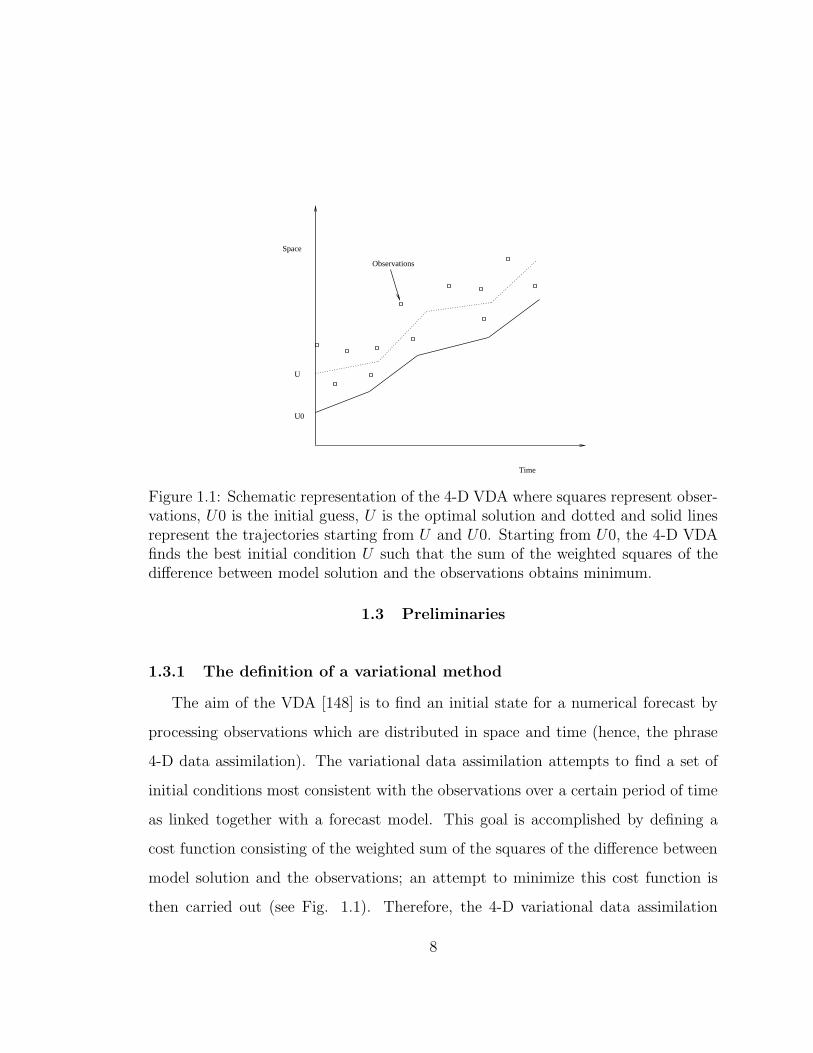
Figure 1.1: Schematic representation of the 4-D VDA where squares represent obser-vations, U0 is the initial guess, U is the optimal solution and dotted and solid linesrepresent the trajectories starting from U and U0. Starting from U0, the 4-D VDAfinds the best initial condition U such that the sum of the weighted squares of thedifference between model solution and the observations obtains minimum.
1.3 Preliminaries
1.3.1 The definition of a variational method
The aim of the VDA [148] is to find an initial state for a numerical forecast by
processing observations which are distributed in space and time (hence, the phrase
4-D data assimilation). The variational data assimilation attempts to find a set of
initial conditions most consistent with the observations over a certain period of time
as linked together with a forecast model. This goal is accomplished by defining a
cost function consisting of the weighted sum of the squares of the difference between
model solution and the observations; an attempt to minimize this cost function is
then carried out (see Fig. 1.1). Therefore, the 4-D variational data assimilation
8
problem may be mathematically defined as
minU
J(U), (1.1)
where the cost function J(U) is defined as
J(U) = Jo + Jb + Jp, (1.2)
where Jo, Jb and Jp are the distance to the observations, the distance to the back-
ground and the penalty term which contains physical constraints applied to the
model state ~X, respectively [3, 83, 158, 214]. To perform a 4-D VDA over a time
period, one needs to find the model trajectory which minimizes the misfit between
model solution and the observations over the period, as well as the misfit to a guess
at the initial time. This initial guess ~Xg represents the best estimate of the model
state at the initial time, prior to any collection of observations at and after the initial
time. As in all the operational assimilation schemes, the initial guess ~Xg represents a
summary of all the information on ~X accumulated before the initial time. A natural
distance for observational errors is the sum of weighted squares of the differences
between the model solution and the observations. For simplicity, we assume the cost
function is defined by
J(U) = Jo =1
2
M∑
i=0
< W (C ~Xi − ~Xoi ), (C
~Xi − ~Xoi ) >, (1.3)
where ~Xi is the state variable vector at the i-th time level in a Hilbert space Xwhose inner product is denoted by < ·, · > using either an Euclidean norm or other
suitably defined norms such as an energy norm. M + 1 is the total number of time
levels in the time assimilation window [t0, tf ] where t0 and tf are the initial and final
times and W is a weighting function usually taken to be the inverse of the covariance
matrix of observation errors. The objective function J(U) is the weighted sum of
the squares of the distance between the model solution and available observations
9
distributed in space and time. ~Xoi is the observation vector at the i-th time level,
while the operator C represents a projection operator from the space of the model
solution ~X to the space of observations. The control variable U and the state vector
~X satisfy model equations
∂ ~X
∂t= F ( ~X), (1.4)
~X(t0) = U, (1.5)
where t is the time, and F ∈ C2 is a function of ~X, where C2 denotes a set of twice
continuously differentiable functions.
It is worth noting that the control variable U may consist of initial conditions
and/or boundary conditions or model parameters to be estimated. For mesoscale
numerical weather prediction (NWP) models and for steady state problems the model
equations will be given by F ( ~X) = 0. Once U is defined, Eq (1.4) has an unique
solution, ~X.
In order to determine or at least approximate the optimal solution of Eq. (1.1)
and therefore the optimal associate state of the atmosphere, we first have to set up
an optimality condition. A general optimality condition is given by the variational
inequality [116]
(∇J(U∗), V − U∗) ≥ 0, (1.6)
for all V belonging to a set of admissible control space Uad where ∇J is the gradient
of the cost functional J with respect to the control variable U .
In the case where Uad has the structure of a linear space, the variational inequality
(1.6) is reduced to an equality
∇J(U∗) = 0. (1.7)
The aforementioned 4-D VDA problem (1.1) usually can not be solved analyti-
cally. Fortunately standard procedures [108, 144] exist allowing us to solve it. Among
10
the feasible methods for large-scale unconstrained minimization are (a) the limited
memory conjugate gradient method ([144, 173, 174, 189, 190]); (b) quasi-Newton
type algorithms ([46], [70], [155]); (c) limited-memory quasi-Newton methods such
as LBFGS algorithm ([117], [154]) and (d) truncated-Newton algorithms ([129], [130],
[131], [138], [185, 186]).
These procedures are iterative procedures, i.e. they start from an initial guess U0,
find a better approximation U1 to optimal solution U in the sense of J(U1) ≤ J(U0),
and repeat this minimization process until a prescribed convergence condition is
met (see Fig. 1.2). A common requirement of all these procedures is the need to
explicitly supply the gradient of the cost function with respect the control variables.
The question is therefore: how to numerically determine the gradient ∇UJ? One
theoretical possibility would be to evaluate the components of ∇UJ through finite-
difference approximations of the form ∆J/∆uj, where ∆J is the computed variation
of J resulting from a given perturbation ∆uj of the j-th component uj of U . This
method has been put forward by Hoffman [85, 86, 87] for performing variational
assimilation. But it requires as many model integrations as there are components
in U . Its numerical cost would be totally prohibitive in most situations, especially
for NWP problems where the number of the components of the control variables is
bigger than 105.
With present computer power, the only practical way to implement variational
assimilation is through an appropriate use of the so-called adjoint of the assimilation
model although it is still computational expensive. The adjoint model of a numerical
model basically consists of the equations which govern the temporal evolution of a
small perturbation imposed on a model equation, written in a form particularly
appropriate for the computation of the sensitivities of the output parameters of the
model with respect to input parameters [19, 20, 80, 103, 128, 232]. The use of
adjoint models is an application of the theory of optimization and optimal control
11
U
U0
Figure 1.2: Schematic representation of a minimization process, where ellipses arethe isolines of the cost function J , U0 is the initial guess, U is the optimal solutionand each arrow represents an iteration of the minimization process.
of PDEs, which has been developed in the last twenty years by mathematicians
[116], and which is progressively being applied to various research disciplines. The
principle for deriving adjoint models is based on a systematic use of the chain rule
for differentiation.
1.3.2 Description of the first order adjoint analysis
A cost effective way to obtain the gradient of the cost function with respect to
the control variables is to integrate the first order adjoint (FOA) model backwards
in time from the final time to the initial time of the assimilation window. The theory
and application of the FOA model is discussed by several authors, e. g. Talagrand
and Courtier [202] and Navon et al. [149]. In order to provide a self-contained
comprehensive dissertation and develop the second order adjoint (SOA) theory, we
briefly summarize the theory of the FOA model.
12
Let us consider a perturbation, U ′, on the initial condition U , Eqs (1.4-1.5)
become
∂( ~X + X)
∂t= F ( ~X + X),
= F ( ~X) +∂F
∂ ~XX +
1
2X∗ ∂F
2
∂ ~X2X +O(‖X‖3), (1.8)
~X(t0) + X(t0) = U + U ′, (1.9)
where (·)∗ denotes the complex conjugate transpose, ‖ · ‖ denotes the Euclidean
norm or other suitably defined norm of “·” and X is the resulting perturbation of
the variable ~X. Retaining only the first order term of Eq (1.8), one obtains
∂X
∂t=∂F
∂ ~XX, (1.10)
X(t0) = U ′. (1.11)
Eqs. (1.10)-(1.11) define the tangent linear model equations of Eqs. (1.4-1.5) and
are linear with respect to the perturbation U ′ on the initial condition U . Eq. (1.10)
is called a tangent linear model because the linearization is around a time-evolving
solution, and therefore, the coefficients of the linear model are defined by slopes of
the tangent to the nonlinear model trajectory in phase space.
The Gateaux derivative δJ of the cost function in the direction of U ′ is defined
by
δJ = limα→0
J(U + αU ′) − J(U)
α, (1.12)
which can be expressed as
δJ = ∇UJ · U ′ (1.13)
Eq. (1.13) is, to the first order accuracy, the variation of the distance function J
due to the perturbation U ′ on the initial condition U , i.e.
δJ =M∑
i=0
< W ( ~Xi − ~Xoi ), Xi > . (1.14)
13
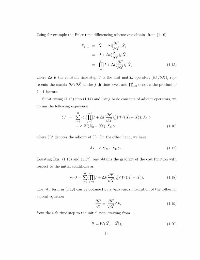
Using for example the Euler time differencing scheme one obtains from (1.10)
Xi+1 = Xi + ∆t[∂F
∂ ~X]iXi
= [I + ∆t(∂F
∂ ~X)i]Xi
=i
∏
j=0
[I + ∆t(∂F
∂ ~X)j]X0 (1.15)
where ∆t is the constant time step, I is the unit matrix operator, (∂F/∂ ~X)j rep-
resents the matrix ∂F/∂ ~X at the j-th time level, and∏i
j=0 denotes the product of
i+ 1 factors.
Substituting (1.15) into (1.14) and using basic concepts of adjoint operators, we
obtain the following expression
δJ =M∑
i=1
< {i−1∏
j=0
[I + ∆t(∂F
∂ ~X)j]}∗W ( ~Xi − ~Xo
i ), X0 >
+ < W ( ~X0 − ~Xo0), X0 > (1.16)
where ( )∗ denotes the adjoint of ( ). On the other hand, we have
δJ =< ∇UJ, X0 > . (1.17)
Equating Eqs. (1.16) and (1.17), one obtains the gradient of the cost function with
respect to the initial conditions as
∇UJ =M∑
i=0
{i−1∏
j=0
[I + ∆t(∂F
∂ ~X)j]}∗W ( ~Xi − ~Xo
i ). (1.18)
The i-th term in (1.18) can be obtained by a backwards integration of the following
adjoint equation
−∂P∂t
= (∂F
∂ ~X)∗P, (1.19)
from the i-th time step to the initial step, starting from
Pi = W ( ~Xi − ~Xoi ), (1.20)
14
where P represents the adjoint variables corresponding to X. It appears that M
integrations of the adjoint model, starting from different time steps tM , tM−1 , ......, t1,
are required to obtain the gradient ∇UJ . However, since the adjoint model (1.19)
is linear, only one integration from tM to t0 of the adjoint equation is required to
calculate the gradient of the cost function with respect to the initial conditions.
In summary, the gradient of the cost function with respect to the initial condition
U can be obtained by the following procedure:
1. Integrate the forecast model from t0 to tM from initial condition (1.5) and store
in memory the corresponding sequence of the model states ~Xi (i =0, 1, ......,
M);
2. Starting from PM = W ( ~XM − ~XoM), integrate the “forced” adjoint equation
(1.19) backwards in time from tM to t0 where a forcing term W ( ~Xi − ~Xoi )
is added to the right-hand-side of (1.19) at the i-th time step whenever an
observation is encountered. The final result P0 is the value of gradient of the
cost function with respect to the initial condition,
∇UJ = P0. (1.21)
It is worth noting that
1. When the observations do not coincide with model grid points, the model
solution should be interpolated to the observations, i.e., C ~X − ~Xo should be
used instead of ~X − ~Xo in the cost function definition, where the operator C
represents the process of interpolating the model solution to space and time
locations where observations are available (i.e. C is a projection operator from
the space of the model solution ~X to the space of observations).
15
2. We note that the numerical cost of the adjoint model computation is about
the same as the cost of one integration of the tangent linear model, the latter
involving a computational cost of at most one integration of the nonlinear
model.
A continuous derivation of the gradient of the cost function is provided Chapter
3. In order to provide the readers with some practical examples and some insight
about the adjoint theory and the accuracies of the TLM, FOA and SOA models,
two examples, one linear and one nonlinear, are presented in Appendices A and
B, respectively. Both examples have exact solutions and thus exactly illustrate the
adjoint process.
1.4 The theme of my dissertation
This thesis is aimed at (a) carrying out a in-depth investigation of the feasibility
of the 4-D VDA applied to realistic situations; (b) achieving an improvement of the
existing large-scale unconstrained minimization algorithms. Toward this end, the
thesis first develops the SOA theory and a modified version of the truncated Newton
(TN) algorithm of Nash [134], secondly develops the SOA model of the shallow-water
equations model and finally derives the FOA model of the Florida State University
global spectral model (FSUGSM), thirdly conducts a series 4-D VDA experiments
and variational nudging data assimilation, and fourthly compares results of the 4-
D VNDA and optimal nudging assimilation to assess their ability to retrieve high
quality model initial conditions (i.e. physical initialization).
The first part of my thesis (Chapters 2, 3) focuses on the development of the
SOA theory and its application. The SOA model serves to study the evolution of
the condition number of the Hessian during the course of the minimization since
one forward integration of the nonlinear model and the tangent linear model and
16
one backwards integration in time of the first order adjoint (FOA) model and the
SOA system are required to provide the value of Hessian/vector product. This Hes-
sian/vector product may then be used with the power method to obtain the largest
and smallest eigenvalues of the Hessian whose dimension is 1083×1083 for our test
problem. The dimension of the Hessian will be more than 105×105 for 3-D primitive
equations models. If the smallest eigenvalues of the Hessian of the cost function
with respect to the control variables are positive at each iteration of the VDA min-
imization process, then the optimal solution of the VDA is unique. This statement
is proved to be true for the shallow water equations model (Subsection 2.4.2). The
variation of the condition number of the Hessian of the cost function with respect to
number of iterations during the minimization process reflects the convergence rate
of the minimization. It has been observed [149] that large scale changes occur in
the process of minimization during the first 30 iterations, while during the ensuing
iterations only small scale features are assimilated. This entails that the condition
number of the Hessian of the cost function with respect to the initial conditions
experiences a fast change at the beginning of the minimization and then remains al-
most unchanged during the latter iterations. The condition number can also provide
information concerning the error covariance matrix. The rate at which algorithms
for computing the best fit to data converge depends on the size of the condition
number as well as the distribution of eigenvalues in the spectrum of the Hessian.
The inverse of the Hessian can be identified as the covariance matrix that establishes
the accuracy to which the model state is determined by the data; the reciprocals of
the Hessian’s eigenvalues represent the variance of linear combinations of variables
determined by the eigenvectors [205]. The above mentioned Hessian/vector product
calculation strategy can be efficiently used in the truncated-Newton algorithm of
Nash [133], which is referred to as adjoint truncated-Newton algorithm (ATN). The
ATN differs from the truncated-Newton algorithm of Nash [134] only in the use of a
17
more accurate Hessian/vector product for carrying out the large-scale unconstrained
optimization required in variational data assimilation. The Hessian/vector product
is obtained by solving an optimal control problem of distributed parameters and its
accuracy is analyzed and compared with its finite-difference counterpart. The ATN
is based on the first and second order adjoint (SOA) techniques allowing to obtain
a better approximation to the Newton line search direction for the problem tested
here. The ATN is applied here to a limited-area shallow water equations model with
model generated data where the initial conditions serve as control variables. We com-
pare the performance of the ATN algorithm with that of the original TN Nash [134]
method and the LBFGS method of Liu and Nocedal [117]. Our numerical tests yield
results which are twice as fast as these obtained by the TN algorithm both in terms
of number of iterations as well as in terms of CPU time. Further the ATN algorithm
turns out to be faster than the LBFGS method in terms of CPU time for the problem
tested.
The second part of my thesis (Chapters 3, 4) addresses the challenging issues
related to 4-D VDA application in NWP problems, i.e. the numerical feasibility
of 4-D variational data assimilation applied to complex NWP models. In order to
address these questions, I choose the FSUGSM as an experimental model, since it is
an operational model developed from the Canadian spectral model of the Recherche
en Prevision Numerique [40] by a research group led by Krishnamurti at Florida
State University. In the development of the FSUGSM from the Canadian model,
the primary effort has been directed at improving the physical effect parameteriza-
tions, adapting the model code to run efficiently on the NCAR Cray-1 computer and
developing post-forecast diagnostics [162]. The FSUGSM is a very complex model.
Developing its first order adjoint model and tuning the minimization algorithm to
perform adequately with a control variable vector of dimension 303104 constitute a
challenging task.
18
In this part of the thesis the tangent linear model (TLM) is first developed and
then the the first order adjoint model (FOA) of the FSUGSM is developed by writing
the TLM backwards in time subroutine by subroutine. The accuracy of the TLM is
investigated by comparing its results with those produced by identical perturbations
introduced in nonlinear forecasts of the original model. The accuracy of the FOA is
verified by using a Taylor expansion.
Through different initial conditions and different scenarios of sets of observations
distributed in time, we demonstrate the efficiency of the 4-D VDA in extracting the
information contained in the dynamics of the model together with the information
contained in the observations. The conditioning is an important factor for an opera-
tional implementation. The dynamics of the model may lead to different reductions
of rms errors at different times and the loss of the conditioning of the problem, i.e.
the shape of the cost function can become strongly elliptic with respect to the non
optimal metric used and the gradient can even become almost orthogonal to the
direction of the minimum. The solution to this is a knowledge of the structure of
the Hessian of the cost function. It seems that the SOA application may constitute
an efficient way to to obtain additional information about the Hessian of the cost
function.
As mentioned before, an implicit assumption made in 4-D VDA is that the model
exactly represents the state of the atmosphere. However, this is clearly not true since
any model only approximately represents the state of the atmosphere. The nudging
data assimilation (NDA) addresses the imperfectness of the model by adding a non-
physical diffusion-type term to the model equations and thus relaxes the model state
towards the observations during the assimilation period (hence an equivalent name
for it is Newtonian relaxation [98, 99]). The NDA method is a flexible assimilation
technique which is computationally much more economical than the VDA method.
However, results from NDA are quite sensitive to the ad hoc specification of the
19
nudging relaxation coefficient, and it is not at all clear how to choose a nudging
coefficient so as to obtain an optimal solution.
Variational nudging data assimilation (VNDA) combines the aforementioned data
assimilation schemes in the most efficient way. It takes both the initial conditions
and the nudging coefficients as control variables and finds the best initial conditions
and optimal nudging coefficients iteratively. In Chapter 6, the VNDA is applied,
in the framework of 4-dimensional variational data assimilation (VDA), to a T42
version of the FSU global spectral model (FSUGSM) in its full-physics operational
form with 12 vertical layers. The technique is tested for its ability to obtain the
best initial conditions and optimal nudging coefficients. Results from the VNDA
indicate significantly better results and a faster convergence rate compared with the
VDA for our test problem when a nudging term is added to the model equations
and the nudging coefficients are optimally estimated using VDA in a parameter es-
timation mode. The humidity and all the different parameterizations of the physical
processes are not included in the adjoint model integration. Thus the calculation of
the gradients by the adjoint model is approximate since the forecast model is used
in its full-physics operational form. It is important to note that the approximate
gradient obtained from a simplified adjoint model is used in the experiments. It is
shown that it is possible to perform variational data assimilation of realistic forecast
models even before more complex adjoint models including diabatic processes are
developed. The resulting optimal nudging coefficients are then applied in nudging
data assimilation (thus the term optimal nudging data assimilation (ONDA)) [229].
Results of data-assimilation experiments involving estimated nudging assimilation,
ONDA and VDA are compared for their ability to retrieve high quality model initial
conditions (physical initialization).
Conclusions summarizing the main results of this thesis, their implications, limi-
tation and outstanding problems are presented in the last Chapter.
20
CHAPTER 2
SECOND ORDER ADJOINT ANALYSIS: THEORY AND
APPLICATIONS
2.1 Introduction
The complete description of the initial atmospheric state in a numerical weather
prediction method constitutes an important issue. The four dimensional variational
data assimilation (VDA) method offers a promising way to obtain such a description
of the atmosphere. It consists in finding the assimilating model solution which min-
imizes a properly chosen objective function measuring the distance between model
solution and available observations distributed in space and time. The control vari-
ables are either the initial conditions or the initial conditions plus the boundary
conditions. The boundary conditions have to be specified so that the problem is well
posed in the sense of Hadamard. In most unconstrained minimization algorithms as-
sociated with the VDA approach, the gradient of the objective function with respect
to the control variables plays an essential role. This gradient is obtained through
one direct integration of the nonlinear model equations followed by a backwards
integration in time of the linear adjoint system of the direct model.
The knowledge of the structure of the Hessian of the cost function with respect to
the control variables is useful in many ways. For instance, the positive definiteness
of the Hessian implies the uniqueness of the solution, the Hessian/vector produc-
tion can be used implement truncated-Newton algorithms [134] and the eigenvalue
distribution and eigenvalue structure of the Hessian can provide useful information
for preconditioning unconstrained minimization algorithms [187]. In this chapter I
21
will develop the SOA theory to study the evolution of the condition number of the
Hessian during the course of the minimization and to conduct the sensitivity analysis
of the cost function with respect to distributed observations.
The context of this chapter is outlined as follows: the theory of the SOA is
introduced in Section 2.2. In Section 2.3, we present a detailed derivation of the
SOA model of a two dimensional shallow water equations model. Quality control
methods for the verification of the correctness of the SOA model are discussed in
Subsection 2.3.1. Issues concerning uniqueness of the solution and the evolution of
the condition number of the Hessian during the course of the minimization as well
as issues related to the structure of the retrieved initial conditions are addressed in
Section 2.4. Section 2.5 is devoted to a sensitivity study of the solution with respect
to distributed inaccurate observations. Finally conclusions are presented in Section
2.6.
2.2 The second order adjoint model
2.2.1 Theory of the second order adjoint model
The forward and backwards integrations of the nonlinear model and its adjoint
model respectively, provide the value of the cost function J and its gradient. The
following question may then be posed: can we obtain any information about the
Hessian (second order derivative matrix) of the cost function with respect to the ini-
tial conditions by integrating the adjoint model equations? Once the Hessian/vector
product is available, the condition number of the Hessian may be obtained. This
condition number may then be used to study the convergence rate of the minimiza-
tion algorithms used in of VDA. We will show in this section that one integration
of the SOA model yields a Hessian/vector product or a column of the Hessian of
the cost function with respect to the initial conditions. Therefore, the SOA model
22
provides an efficient way to compute the Hessian of the cost function by performing
M integrations of the SOA model where M is the number of the components in the
control variables. For a large dimensional model, obtaining the full Hessian matrix
proves to be a computationally prohibitive task beyond the capability of present
day computers. The SOA approach will be used to conduct a sensitivity analysis
of the observations in Section 2.5. We will also study the relative importance of
observations distributed at different space and time locations.
The original idea of the SOA theory was proposed by Le Dimet (personal com-
munication). Here we developed the SOA theory in a clearer and simple manner.
Assume that the model equations are given by Eqs. (1.4) and (1.5). Let us define
the cost function as
J(U) =1
2
∫ T
t0
< W (C ~X − ~Xo), C ~X − ~Xo > dt, (2.1)
where W is a weighting matrix often taken to be the inverse of the estimate of the
covariance matrix of the observation errors, T is the final time of the assimilation
window, the objective function J(U) is the weighted sum of squares of the distance
between model solution and available observations distributed in space and time,
~Xo is observation vector, the projection operator C represents the process of inter-
polating the model solution ~X to space and time locations where observations are
available. The purpose is to find the initial conditions such that the solution of the
Eq. (1.4) minimizes the cost function J(U) in a least-squares sense. The FOA model
as defined by Eqs. (1.19)-(1.20) may then be rewritten as
−∂P∂t
= (∂F
∂ ~X)∗P + C∗W (C ~X − ~Xo), (2.2)
P (T ) = 0. (2.3)
23
where P represents the FOA variables vector. The gradient of the cost function with
respect to the initial conditions is given by (see Subsection 3.2.1)
∇UJ = P (t0), (2.4)
Let us now consider a perturbation, U ′, on the initial condition U . The resulting
perturbations for the variables ~X, P , X and P may be obtained from Eqs. (1.4)-(1.5)
and (2.2)-(2.3) as
∂X
∂t=∂F
∂ ~XX, (2.5)
X(0) = U ′, (2.6)
−∂P∂t
= (∂F
∂ ~X)∗P + [
∂2F
∂ ~X2X]∗P + C∗WCX, (2.7)
P (T ) = 0, (2.8)
Eqs. (2.5)-(2.6) and Eqs. (2.7) and (2.8) are called the tangent linear and SOA
models, respectively.
Let us denote the FOA variable after a perturbation U ′ on the initial condition
U by PU+U ′, then according to definition
PU+U ′(t0) = P (t0) + P (t0). (2.9)
Expanding ∇U+U ′J at U in a Taylor series and only retaining the first order term,
results in
∇U+U ′J = ∇UJ + ∇2J · U ′ +O(‖U ′‖2) (2.10)
From Eq. (2.4), we know that
∇U+U ′J = PU+U ′(t0), (2.11)
Combining Eqs. (2.4), (2.9), (2.10) and (2.11), one obtains
P (t0) = ∇2J · U ′ = HU ′, (2.12)
24
where H = ∇2J is the second derivative of the cost function with respect to initial
conditions.
If we set U ′ = ej, where ej is the unit vector with the j-th element equal to 1,
the j-th column of the Hessian may be obtained by
Hej = P (t0) (2.13)
Therefore theoretically speaking, the full Hessian H can be obtained by M integra-
tions of Eqs. (2.7)-(2.8) with U ′ = ei, i = 1, ...,M where M is the number of the
components of the control variables (the initial conditions u(t0), v(t0) and φ(t0) in
our case).
In summary, the j-th column of the Hessian of the cost function can be obtained
by the following procedure (also see Fig. 2.1):
1. Integrate the model (1.4)-(1.5) and the tangent linear model (2.5)-(2.6) forward
and store in memory the corresponding sequences of the states ~Xi and Xi (i
=0, ......, M);
2. Integrate the FOA equations (2.2)-(2.3) backwards in time and store in memory
the sequence of Pi (i =0, ......, M);
3. Integrate the SOA model (2.7)-(2.8) backwards in time. The final value P (t0),
yields the j-th column of the Hessian of the cost function with respect to the
control variables.
2.2.2 The estimate of the condition number of the Hessian
Let us denote the largest and the smallest eigenvalues of the Hessian of the cost
function with respect to the control variables and their corresponding eigenvectors
by λmax, λmin, Vmax and Vmin, respectively. Then the condition number of the Hessian
25
is given by
κ(H) =λmax
λmin(2.14)
Considering the eigenvalue problem HU = λU and assuming that the eigenvalues
are ordered in decreasing order with |λ1| ≥ |λ2| ≥.......≥ |λn|, an arbitrary initial
vector X0 may be expressed as a linear combination of the eigenvectors {Ui}
X0 =n
∑
i=1
ciUi (2.15)
If λi is an eigenvalue corresponding to the i-th eigenvector Ui, m times multiplications
of the Hessian H to (2.15) result in,
Xm =n
∑
i=1
ciλmi Ui, (2.16)
where
Xm = HmX0. (2.17)
Factoring λm1 out, we obtain
Xm = λm1
n∑
i=1
ci(λi
λ1)mUi. (2.18)
Since λ1 is the largest eigenvalue, the ratio (λi/λ1)m approaches zero as m increases
(suppose λ1 6= λ2). Therefore we may write
Xm = λm1 c1U1, (2.19)
From (2.19) we observe that the largest eigenvalue may be calculated by
λ1 =jth component of Xm+1
jth component of Xm
(2.20)
This technique is called the power method [199]. We can normalize the vector Xm
by its largest component in absolute value. If we denote the new scaled iterate by
X ′m, then
Xm+1 = HX ′m, (2.21)
26
and the method is called the power method with scaling. It yields an eigenvector
whose largest component is 1.
The main steps in the power method algorithm with scaling are:
1. Generate a starting vector X0.
2. Form a matrix power sequence Xm = HXm−1.
3. Normalize Xm so that its largest component is unity.
4. Return to step (b) until convergence
|Xm −Xm−1| ≤ 10−6, (2.22)
is satisfied or a prescribed upper limit of the number of iterations has been attained.
The smallest eigenvalue of H may also be computed by applying the shifted
iterated power method to the matrix Z = z · I −H, where z is the majorant of the
spectral radius of H and I the identity matrix.
2.3 The derivation of the second order adjoint model for the shallow
water equations model
In this section, we consider the application of the SOA model to a two dimensional
limited-area shallow water equations model. Our purpose is to illustrate how to
derive the SOA model explicitly.
The shallow water equations model may be written as
∂u
∂t= −u∂u
∂x− v
∂u
∂y+ fv − ∂φ
∂x, (2.23)
∂v
∂t= −u∂v
∂x− v
∂v
∂y− fu− ∂φ
∂y, (2.24)
∂φ
∂t= −∂(uφ)
∂x− ∂(vφ)
∂y, (2.25)
27
where u, v, φ and f are the two components of the horizontal velocity and geopo-
tential fields and the Coriolis factor, respectively.
We shall use initial conditions due to Grammeltvedt [75]
h = H0 +H1tanh9(y − y0)
2D+H2sech
9(y − y0)
Dsin
2πx
L, (2.26)
where H0 = 2000m, H1 = −220m, H2 = 133m, g = 10msec−2, L = 6000km,
D = 4400km, f = 10−4sec−1, β = 1.5 × 10⁻¹¹sec−1m−1. Here L is the length of the
channel on the β plane, D is the width of the channel and y0 = D/2 is the middle of
the channel. The initial velocity fields were derived from the initial height field via
the geostrophic relationship, and are given by
u = − gf
∂h
∂y, (2.27)
v =g
f
∂h
∂x. (2.28)
The time and space increments used in the model are
∆x = 300km, ∆y = 220km, ∆t = 600s, (2.29)
which mean that there are 21×21 grid point locations in the channel and the number
of the components of initial condition vector (u, v, φ)t is 1083. Therefore the Hessian
of the cost function in our test problem has a dimension of 1083×1083.
The southern and north boundaries are rigid walls where the normal velocity
components vanish, and it is assumed that the flow is periodic in the west-east
direction with a wave length equal to the length of the channel.
Let us define
~X = (u, v, φ)T , (2.30)
F = −
u∂u∂x
+ v ∂u∂y
− fv + ∂φ
∂x
u∂v∂x
+ v ∂v∂y
+ fu+ ∂φ
∂y
∂(uφ)∂x
+ ∂(vφ)∂y
. (2.31)
28
Then Eqs. (2.23)-(2.25) assume the form of Eq. (1.4). It is easy to verify that
∂F
∂ ~X= −
∂(u(·))∂x
+ v ∂(·)∂y
(·)∂u∂y
− f(·) ∂(·)∂x
(·)∂v∂x
+ f(·) u∂(·)∂x
+ ∂(v(·))∂y
∂(·)∂y
∂(φ(·))∂x
∂(φ(·))∂y
∂(u(·))∂x
+ ∂(v(·))∂y
. (2.32)
The adjoint of an operator L, L∗ is defined by the relationship
< L ~X, ~Y >=< ~X,L∗~Y >, (2.33)
where < ·, · > denotes the inner product
< ·, · >=∫ ∫
D· · dD, (2.34)
where D is the spatial domain. Using the definition (2.34), the adjoint of (2.33) can
be derived as
[∂F
∂ ~X]∗ = −
−u∂(·)∂x
− ∂(v(·))∂y
(·)∂v∂x
+ f(·) −φ∂(·)∂x
(·)∂u∂y
− f(·) −v ∂(·)∂y
− ∂(u(·))∂x
−φ∂(·)∂y
−∂(·)∂x
−∂(·)∂y
−u∂(·)∂x
− v ∂(·)∂y
. (2.35)
Therefore the first order adjoint model with the forcing terms may be written as
−∂u∗
∂t= −(−u∂u
∗
∂x− ∂(vu∗)
∂y+ v∗
∂v
∂x+ fv∗ − φ
∂φ∗
∂x) +Wu(u− uo), (2.36)
−∂v∗
∂t= −(u∗
∂u
∂y− fu∗ − v
∂v∗
∂y− ∂(uv∗)
∂x− φ
∂φ∗
∂y) +Wv(v − vo), (2.37)
−∂φ∗
∂t= −(−∂u
∗
∂x− ∂v∗
∂y− u
∂φ∗
∂x− v
∂φ∗
∂y) +Wφ(φ− φo), (2.38)
with final conditions
u(T ) = 0, v(T ) = 0, φ(T ) = 0, (2.39)
where P = (u∗, v∗, φ∗)t is the first order adjoint variable. Wu,Wv,Wφ are weighting
factors which are taken to be the inverse of estimates of the statistical root-mean-
square observational errors on geopotential and wind components respectively. In
our test problem, values of Wφ = 10−4m−4s4 and Wu = Wv = 10−2m−2s2 are used.
29
Now let us consider a perturbation, U ′, on the initial condition for ~X, ~X(t0).
The resulting corresponding perturbations for variables ~X and P , X = (u, v, φ)t and
P = (u, v, φ)t, are obtained from Eqs. (2.23)-(2.25) and (2.36)-(2.39) as
∂u
∂t= −(
∂(uu)
∂x+ v
∂u
∂y+ v
∂u
∂y− f v +
∂φ
∂x), (2.40)
∂v
∂t= −(u
∂v
∂x+ fu+ u
∂v
∂x+∂(vv)
∂y+∂φ
∂y), (2.41)
∂φ
∂t= −(
∂(φu)
∂x+∂(φv)
∂y+∂(uφ)
∂x+∂(vφ)
∂y), (2.42)
with zero initial conditions, and
−∂u∂t
= −(−u∂u∂x
− ∂(vu)
∂y+ v
∂v
∂x− φ
∂φ
∂x−
u∂u∗
∂x− ∂(vu∗)
∂y+ v∗
∂v
∂x− φ
∂φ∗
∂x) +Wuu, (2.43)
−∂v∂t
= −(u∂u
∂y− v
∂v
∂y− ∂(uv)
∂x− φ
∂φ
∂y+
u∗∂u
∂y− v
∂v∗
∂y− ∂(uv∗)
∂x− φ
∂φ∗
∂y) +Wvv, (2.44)
−∂φ∂t
= −(−∂u∂x
− ∂v
∂y− u
∂φ
∂x− v
∂φ
∂y−
u∂φ∗
∂x− v
∂φ∗
∂y) +Wφφ, (2.45)
with final condition
u(T ) = 0, v(T ) = 0, φ(T ) = 0. (2.46)
Therefore
P (t0) = (u(t0), v(t0), φ(t0))t = HU ′, (2.47)
where H is the Hessian of the cost function with respect to the initial conditions (the
control variables). Equation (2.47) gives the Hessian/vector product. If we choose
30
U ′ to be unit vector ej where the j-th component is unity and all other components
are zeros, then the corresponding column Hj of the Hessian H will be obtained after
one integration of the SOA backwards in time.
2.3.1 The verification of the correctness of the first and the second order
adjoint models
It is very important to verify the correctness of the FOA and SOA codes. A
Taylor expansion in the ~Y direction leads to
J( ~X + α~Y ) = J( ~X) + α∂J( ~X)
∂ ~X~Y +
1
2α2~Y t∂
2J( ~X)
∂ ~X2~Y +O(α3), (2.48)
where α is a small scalar, ~Y is a random perturbation vector which can be generated
by using the randomizer on the Cray-YMP computer and ~Y t denotes the transpose
of the vector ~Y . Equation (B.1) can be used to define two functions of α
ψ(α) =J( ~X + α~Y ) − J( ~X)
α∂J( ~X)
∂ ~X~Y
, (2.49)
and
φ(α) =J( ~X + α~Y ) − J( ~X) − α ∂J( ~X)
∂ ~X~Y
12α2~Y t ∂2J( ~X)
∂ ~X2
~Y, (2.50)
then for small α we have
ψ(α) = 1 +O(α), (2.51)
φ(α) = 1 +O(α), (2.52)
For values of α which are small but not very close to the machine zero, one should
expect a value of ψ(α) or φ(α) approaching 1 linearly for a wide range of magnitudes
of α.
The experiment was performed using a limited area 2-D shallow water equation
model. The results are shown in Figure 2.2. It is clearly seen that for values of α
between 100-10−11 unit values for ψ(α) and φ(α) are obtained. The correctness of
31
the gradient of the cost function and the correctness of the Hessian/vector product
have therefore been verified.
2.4 Second order adjoint information
2.4.1 Calculation of the Hessian/vector product
There are two practical ways to calculate the Hessian/vector product at a point ~X
associated with VDA. One way consists in using a finite difference method while the
other way is the SOA method. The finite-difference approach assumes the following
form (namely a difference between two adjacent gradient values)
f(α) = ∇J( ~X + α~Y ) −∇J( ~X) = αH~Y +O(α2), (2.53)
where ~Y is a random perturbation vector and H is the Hessian of the cost function.
A second way to obtain Hessian/vector product is to integrate the SOA equations
model backwards in time. According to Eq. (2.12), we also have
f(α) = αH~Y , (2.54)
The computational cost required to obtain the Hessian/vector product is approx-
imately the same for both methods. The SOA approach requires us to integrate
the original nonlinear model and its tangent linear model forward in time once and
integrate the FOA model and the SOA model backwards in time once. The finite
difference approach requires the integration of the original nonlinear model forward
in time and the FOA model backwards in time twice. The computational costs for
integrating the tangent linear model forward in time, or the FOA model backwards
in time and the SOA model backwards in time once are comparable. However the
SOA model method gives an accurate value of the Hessian/vector product while the
finite-difference method yields only an approximate value, which can be a very poor
32
estimate when the value α is not properly chosen. Figures 2.3, 2.4, 2.5 presents a
comparison between the first 50 components of Hessian/vector products at the opti-
mal point obtained by using both the SOA and finite-difference approaches for various
scalars α varying from 10, 3 to 0.01. It is clearly seen that the Hessian/vector product
obtained by using finite-difference approach converges to that obtained by SOA as the
scalar α decreases. With the SOA approach a more accurate result can be obtained
with a relatively large perturbation (α = 10), while the finite-difference approach is
much more sensitive to the magnitude of perturbations. When the perturbations are
large, say for α = 10, the finite-differencing approach yields no meaningful results
(Figure 2.3). When the perturbations are small, the finite-difference approach might
involve a subtraction of nearly equal numbers which results in the cancellation of
significant digits and the results thus obtained are an inaccurate estimate of the Hes-
sian/vector product. This is the case when the Hessian/vector product is estimated
at the initial guess point with α = 0.01 (Figure 2.6). Therefore it is much more
advantageous to use the SOA approach than to use the finite-difference approach.
The calculation of a Hessian/vector product is required in many occurrences.
For instance, Nash’s Truncated Newton method [130] requires the values of Hes-
sian/vector products. It may also be used to carry out eigenvalue calculations and
sensitivity analyses.
2.4.2 The uniqueness of the solution
An important issue related to VDA application is to determine whether the solu-
tion obtained is unique. If there is more than one local minimum, then the solution
obtained by the minimization process may possibly change depending on different
initial guesses.
There are two different but complementary ways to characterize the solution to
unconstrained optimization problems. In the local approach, one examines the rela-
33
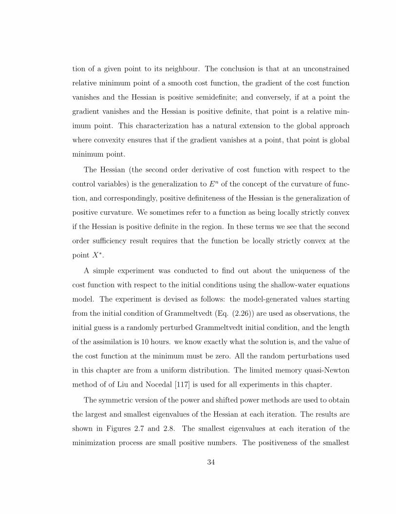
tion of a given point to its neighbour. The conclusion is that at an unconstrained
relative minimum point of a smooth cost function, the gradient of the cost function
vanishes and the Hessian is positive semidefinite; and conversely, if at a point the
gradient vanishes and the Hessian is positive definite, that point is a relative min-
imum point. This characterization has a natural extension to the global approach
where convexity ensures that if the gradient vanishes at a point, that point is global
minimum point.
The Hessian (the second order derivative of cost function with respect to the
control variables) is the generalization to En of the concept of the curvature of func-
tion, and correspondingly, positive definiteness of the Hessian is the generalization of
positive curvature. We sometimes refer to a function as being locally strictly convex
if the Hessian is positive definite in the region. In these terms we see that the second
order sufficiency result requires that the function be locally strictly convex at the
point X∗.
A simple experiment was conducted to find out about the uniqueness of the
cost function with respect to the initial conditions using the shallow-water equations
model. The experiment is devised as follows: the model-generated values starting
from the initial condition of Grammeltvedt (Eq. (2.26)) are used as observations, the
initial guess is a randomly perturbed Grammeltvedt initial condition, and the length
of the assimilation is 10 hours. we know exactly what the solution is, and the value of
the cost function at the minimum must be zero. All the random perturbations used
in this chapter are from a uniform distribution. The limited memory quasi-Newton
method of of Liu and Nocedal [117] is used for all experiments in this chapter.
The symmetric version of the power and shifted power methods are used to obtain
the largest and smallest eigenvalues of the Hessian at each iteration. The results are
shown in Figures 2.7 and 2.8. The smallest eigenvalues at each iteration of the
minimization process are small positive numbers. The positiveness of the smallest
34
eigenvalues implies positive definiteness of the Hessian, which in turn proves the
uniqueness of the optimal solution.
2.4.3 Convergence analysis
The largest and smallest eigenvalues and the condition numbers are considered
here. The purpose of this study is to provide an in-depth diagnosis of the conver-
gence of the VDA applied to a meteorological problem. The various scale changes
of different field retrievals with the number of minimization iterations of VDA have
attracted the attention of several researchers [149]. In this research work we will
attempt to provide an explanation of this phenomenon based on the evolution of the
condition number of the Hessian of the cost function with respect to control variables
[205]. It has been observed that in VDA large scale changes occur in the first few
iterations and small scale changes occur during the latter iterations in the process of
the minimization of the cost function.
The same experiment as described in section 4.2 was conducted again this time
to follow the quality of the retrievals initial conditions at different stages of the
minimization process. Figures 2.9-2.11 show the perturbed geopotential field and
the retrieved geopotential fields after 6 and 25 iterations, respectively. It can be
clearly seen that most of the large scale retrievals occur within the first 25 iterations
of the minimization process. The geopotential field retrieved after 25 iterations is
very similar to the one retrieved after 54 iterations at which stage the prescribed
convergence criterion
‖∇J( ~Xk)‖ ≤ 10−14 ×max{1, ‖ ~Xk‖}, (2.55)
is satisfied. This clearly indicates that the VDA achieves most of the large scale
retrievals during the first 25 iterations and that in the latter part of the minimization
process only small scale features are being assimilated. In this case by stopping the
minimization process prior to the cost function satisfying the preset convergence
35

criteria, the expensive computational cost of the VDA process could be cut by more
than a half, while satisfactory results may still be obtained.
This in turn is related to the evolution of the largest and smallest eigenvalues of
the Hessian spectrum and thus to the change in the condition number of the Hessian
with the number of iterations (Figures 2.7, 2.8 and 2.12). From these figures we
observe
1. The smallest eigenvalues are positive at each iteration and remain approxi-
mately the same except for rather small changes during the first a few iterations
(Figure 2.7).
2. The largest eigenvalues decrease quickly during the first a few iterations of
the minimization process, then change only slightly for the next 15 iterations
and finally remain approximately the same until the convergence criteria are
attained (Figure 2.8).
3. The condition numbers of the Hessian/vector product at different steps of the
minimization vary in a way similar to the evolution of the largest eigenvalues
during the minimization process and they are around 83,000 in magnitude
which is very large (Figure 2.12).
We see now that most changes in the condition numbers occur during the early
stage of the VDA minimization process. This explains why large scale retrievals
occur during the first few (25-30) iterations of the minimization process.
The large condition numbers in the initial stage of the minimization imply that
the contour lines of the cost function J = constant are strongly elongated in the
parameter space [62, 73, 116, 123], which explains the slow convergence rate of the
VDA process. The above experiment was carried out without adding either a penalty
or a smoothing term. The addition of such a penalty term, which is positive definite
36
and quadratic with respect to the initial conditions, will definitely increase the con-
vexity of the cost function. Thus the addition of an adequate quadratic penalty term
adding additional information to the cost function changes the condition number of
the Hessian and speeds up the convergence of the VDA process.
2.5 Sensitivity analysis for observations
2.5.1 Sensitivity theory for observation
The cost function is also a function of the observations. Different observations
will result in different solutions. Due to the errors inherent in the heterogeneous ob-
servations, it is important to obtain the sensitivities of the cost function to changes in
the observations which quantify to what extent the perturbations in the observations
correspond to the perturbation in the solution. If the sensitivities are large, then the
model will possess a large uncertainty with respect to changes in the observations.
Conventional evaluation of the sensitivities with respect to model parameters is
carried out by changing the values of model parameters and recalculating each model
solution for every parameter. Such a calculation is prohibitive for models with a large
number of parameters since it requires an exceedingly large amount of computing
time. The adjoint sensitivity method [19, 20, 78, 79, 200] has proved to be an efficient
way for carrying out sensitivity analysis. The objective of the sensitivity analysis
considered here is to estimate changes in the cost function J arising from changes in
observations which are distributed in space and time. This will illustrate the relative
importance of observations at different time and space locations.
Assume that the operator C in Eq. (2.1) is an unit operator. Due to the equivalent
position of the state vector and the observation vector in Eq. (2.1), the cost function
can be viewed as depending on both of them, namely
J = J( ~X − ~Xo), (2.56)
37
As such, the following identities can be proved using the chain rule:
∂J
∂ ~X= − ∂J
∂ ~Xo, (2.57)
∂2J
∂ ~X2=
∂2J
∂ ~Xo2 , (2.58)
These two equations are used in the following sensitivity analysis.
Let us denote a change in the observations by δ ~Xo. If this change is small, then
we may expand the cost function J around ~Xo in a Taylor series as
J( ~Xo(tn) + δ ~Xo(tn)) = J( ~Xo(tn)) +∂J( ~Xo(tn))
∂ ~Xo(tn)δ ~Xo(tn)
+1
2δ ~Xo(tn)t∂
2J( ~Xo(tn))
∂ ~Xo(tn)2δ ~Xo(tn) +O(‖δ ~Xo(tn)‖3), (2.59)
According to the identities given by Eqs. (2.57) and (2.58), Eq. (2.59) can be written
as
J( ~Xo(tn) + δ ~Xo(tn)) = J( ~Xo(tn)) − ∂J( ~Xo(tn))
∂ ~X(tn)δ ~Xo
+1
2δ ~Xo(tn)t∂
2J( ~Xo(tn))
∂ ~X(tn)2δ ~Xo +O(‖δ ~Xo(tn)‖3), (2.60)
where tn denotes the time, tn = t0 + n∆t and ∆t is given by Eq. (2.29). Since the
first order term in Eq. (2.60) dominates, we obtain from Eq. (2.60)
J ′ = J( ~Xo(tn) + δ ~Xo(tn)) − J( ~Xo(tn))
= −∂J( ~Xo(tn))
∂ ~X(tn)δ ~Xo +O(‖δ ~Xo(tn)‖2). (2.61)
This equation describes changes in the cost function resulting from changes in the
observation at time tn.
If the gradient of the cost function with respect to the state vector X(tn) is zero,
then we obtain
J ′ = J( ~Xo(tn) + δ ~Xo(tn)) − J( ~Xo(tn))
=1
2δ ~Xo(tn)t∂
2J( ~Xo(tn))
∂ ~X(tn)2δ ~Xo +O(‖δ ~Xo(tn)‖3), (2.62)
38
where the second derivative of J with respect to the observations is the Hessian of J
with respect to the state variable at time tn. Equation (2.62) describes the changes
in the cost function resulting from a change in the observation at time tn.
The gradient ∂J( ~Xo(tn))/∂ ~X(tn) of the cost function with respect to the state
variable ~X(tn) is the value of the first order adjoint variable at time tn. The Hessian
∂2J( ~Xo(tn))/∂ ~X(tn)2 of the cost function with respect to the state variable ~X(tn)
is not required. Only the Hessian/vector product [∂2J( ~Xo(tn))/∂ ~X(tn)2] ~Xo(tn) is
required and it may be obtained using an integration of the second order adjoint
model Eqs. (2.7) and (2.8).
In summary, the perturbation in the cost function resulting from a perturbation
in the observations at the time tn may be obtained by performing the following
operations provided the gradient of the cost function with respect to the state vector
X(tn) does not vanish.
1. Generate a perturbation on the observation at time tn;
2. Calculate the gradient of the cost function with respect to state variable X(tn),
i.e. starting from PM = W ( ~XM− ~XoM), integrate the “forced” adjoint equation
Pi = [I + ∆t(∂F
∂ ~X)∗i ]Pi+1 +W ( ~Xi − ~Xo
i ), (2.63)
backwards in time from tM to tn. The final result Pn is the gradient of the cost
function;
3. Use equation (2.61) to obtain the corresponding perturbation in the cost func-
tion resulting from the perturbation in the observations at time tn.
If the gradient of the cost function with respect to the state vector X(tn) is close
to zero, then we modify the last two steps as
39
1. Calculate the Hessian/vector product [∂2J( ~Xo(tn))/∂ ~X(tn)2] ~Xo(tn). That is
to integrate the second order adjoint model Eqs. (2.7) and (2.8) backwards in
time from tM to tn. The final result Pn is the required Hessian/vector product;
2. Use equation (2.62) to obtain the corresponding perturbation in the cost func-
tion resulting from the perturbation in the observations at time tn.
It is worthwhile noting that we need not integrate the FOA equations repeatedly
to obtain the gradient of the cost function with respect to ~Xtn . We need only to
integrate the FOA equations backwards in time starting from tM to tn and store the
FOA variable at each iteration in memory. The final value is the gradient of the
cost function with respect to the state variables at time tn. Once these gradients are
calculated, they need not be recalculated. They can be used repeatedly to calculate
the perturbations in the cost function for different perturbations in the observations.
2.5.2 Numerical results from model generated data
A sensitivity study was conducted by using the same model as described in Section
3 and the sensitivity calculations were carried out using formula (5.7) at the end of the
variational data assimilation. First we choose a point (x15 , y10) in the assimilation
window where x15 = x0 + 15∆x and y10 = y0 + 10∆y. Suppose a 1% perturbation
in the observations occurs only at this point for the two components of the wind
velocity field and the geopotential field. The variation of the resulting perturbations
in the cost function as a function of the number of time steps is displayed in Figure
2.13 (solid line). The results indicate that the changes in the cost function with
respect to the changes in the observations at a fixed point are different for different
times in the window of assimilation. If perturbations are imposed first only on the
u−wind component, then only on the v−wind component and then only on the
geopotential field φ, the corresponding perturbations in the cost function exhibit
40
different variations with time as shown in Figure 2.13 by the dotted line, dashed line
and dash-dot line, respectively. This figure indicates also that perturbations in the
observed geopotential field have more impact on the cost function than these in the
observed velocity field. The changes in the cost function arising from changes in the
u-wind component and v-wind component observations are close to zero at all times.
Similar experiments conducted at different grid points yielded similar results.
In order to study the importance of observations at different space locations,
three different points are chosen. They are located at (x5, y15), (x10, y10), (x15, y5),
respectively, representing low, middle and high points in the isoline values of the
geopotential field. From Figure 2.14 we observe that changes in the magnitudes of
the cost function at the three points behave in a similar pattern and the sensitivities
at the three points differ dramatically at the beginning of the assimilation window.
Finally, we study the impact of the perturbations on all the observational data.
The results are displayed in Figure 2.15. This figure clearly indicates that perturba-
tions of the observations at the beginning of the window of assimilation have a larger
impact on the sensitivity of the cost function with respect to the observations.
Presented in Table 1 are sensitivities (the column labeled “Predicted change”) of
the cost function due to 1% changes in the observations at the beginning of the assim-
ilation window and the corresponding actual changes (the column labeled “Actual
change”) obtained by rerunning the model after actually varying the observations
by 1%. The good agreement obtained between the actual and predicted changes as
shown in Table 1 provides evidence as to the adequacy of the numerical method used
to obtain these sensitivities.
41
2.5.3 Numerical results using real analysis of First Global Geophysical
Experiment (FGGE) data
In order to examine the sensitivity of the cost function with respect to real
analyses, we employed a set of FGGE data of height and horizontal wind fields
at 500mb level at 0 and 18UTC, May 26, 1979. The data are equally spaced with
∆λ = ∆φ = 1.875◦. Using the formula
φ(J) =y
α+ φ0 =
−2200 + (J − 1) ∗ 220
α+ φ0, (2.64)
λ(I) =x
α cos φ(J)+ λ0, (2.65)
we obtain a correspondence between points on the sphere and grid points located
on a limited area on a β−plane approximation at (32◦, 130◦), which approximately
represents the center of the zonal jet. Using a cubic interpolation we obtained the
height and horizontal wind data on the grid points. Then we carried out another
cubic interpolation near the left boundary in order to impose a periodic boundary
condition in the x-direction. Near the top and bottom boundaries we used a linear
interpolation to impose solid boundary conditions. The fields thus obtained are
shown in Figure 2.16.
The geopotential and wind fields at time 0UTC were used to produce the model-
generated observations. The minimization started from geopotential and wind fields
distribution at time 18UTC. The difference between these two fields is shown in
Figure 2.17. Having the model generated observations, the minimization should be
able to reduce the value of the cost function as well as the norm of its gradient, and
the retrieved differences should be zero. This turns out to be the case.
The sensitivity calculations were carried out using formulas (2.61) plus (2.62) at
the beginning of the variational data assimilation. From Figure 2.16, we note that
meteorologically intensive events occur at the center area of the limited-area domain
while fewer such events occur at the corners of the limited-area domain. We choose
42
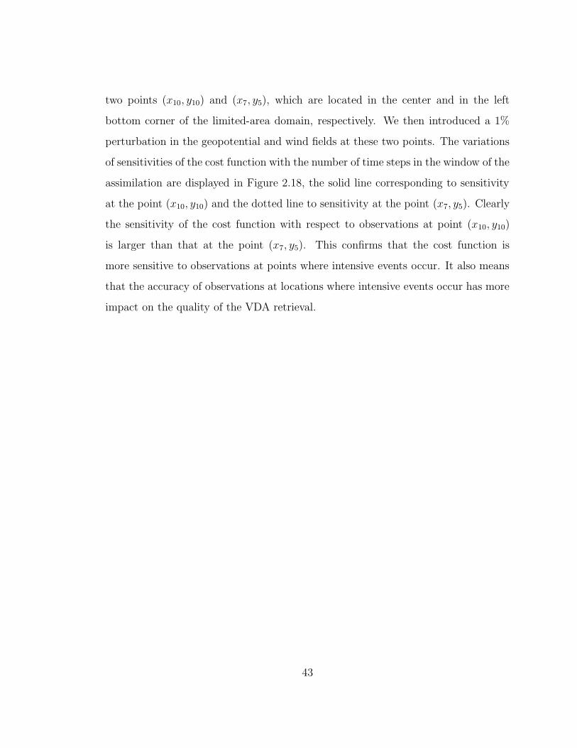
two points (x10, y10) and (x7, y5), which are located in the center and in the left
bottom corner of the limited-area domain, respectively. We then introduced a 1%
perturbation in the geopotential and wind fields at these two points. The variations
of sensitivities of the cost function with the number of time steps in the window of the
assimilation are displayed in Figure 2.18, the solid line corresponding to sensitivity
at the point (x10, y10) and the dotted line to sensitivity at the point (x7, y5). Clearly
the sensitivity of the cost function with respect to observations at point (x10, y10)
is larger than that at the point (x7, y5). This confirms that the cost function is
more sensitive to observations at points where intensive events occur. It also means
that the accuracy of observations at locations where intensive events occur has more
impact on the quality of the VDA retrieval.
43
2.6 Conclusions
In this chapter, a SOA model was developed, providing second order information.
The coding work involving in obtaining the SOA model is rather modest once the
FOA model has been developed.
One integration of the SOA model yields an accurate value of a column of the
Hessian of the cost function with respect to the control variables provided the per-
turbation vector is a unit vector with one component being unity and the rest being
zeros. Numerical results show that the use of the SOA approach to obtain the
Hessian/vector product is much more advantageous than the corresponding finite-
difference approach, since the latter yields only an approximated value of the Hes-
sian/vector product which may be a very poor approximation. The numerical cost
of using the SOA approach is roughly the same as that of using the finite-difference
approach. This application of the SOA model is crucial in the implementation of
the large-scale truncated Newton method, which was proved to be a very efficient
algorithm for large-scale unconstrained minimization [225].
Another application of the SOA model is the calculation of eigenvalues and eigen-
vectors of the Hessian. There are several iterative methods such as the power,
Rayleigh quotient or the Lanczos method [199], which (combined with deflation)
require only information of the Hessian multiplied by a vector to calculate several
dominant eigenvalues and their respective eigenvectors. Such a calculation using the
power method is presented in this chapter and reveals that most changes in the largest
eigenvalue of the Hessian occur during the first few iterations of the minimization
procedure, which may explain why most of large-scale features are retrieved earlier
than the small scale features in the VDA retrieval solution during minimization [149]
while the positiveness of the smallest eigenvalues of the Hessian of the cost function
during the minimization process indicate the uniqueness of the optimal solution.
44
We also examined the sensitivity of the cost function to observational errors using
a two dimensional limited-area shallow water equations model. We found that the
sensitivity depends on the time when the errors occur, the specific field containing
the errors, and the spatial location where these errors occur. The cost function is
more sensitive to observational errors occurring at the beginning of the assimilation
window, to errors in the geopotential field, and to errors at grid point locations where
intensive events occur.
Sensitivity analysis using balanced perturbations will be reported later where we
pay special attention to the spatial scale of the perturbations. Further research on
the issue of calculating the inverse Hessian multiplied by a vector is currently under
consideration, the latter being of crucial importance for developing a new efficient
large-scale unconstrained minimization algorithm.
45
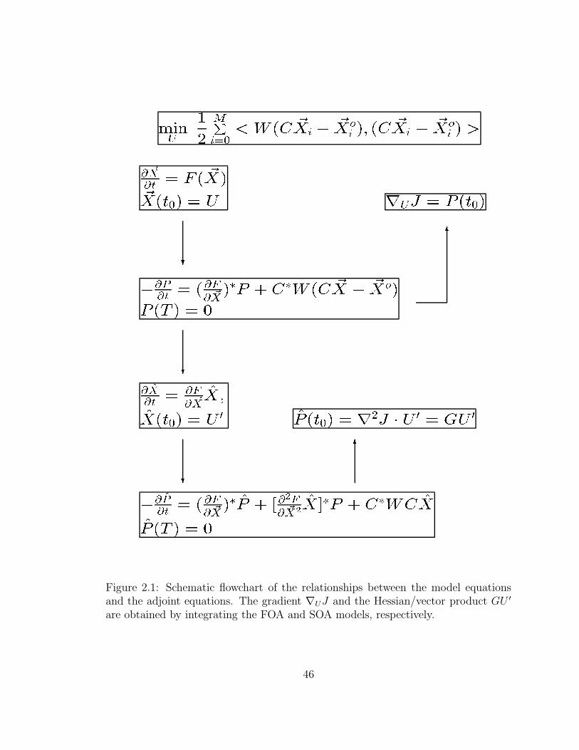
� ������� �� ��� � ��� �� �� �� ����� ��� �� �� �� ��� �
!#"$!&% ' ( �)�� ��� �+* � � ' , - �/. ' 0 �+* � �
12
� !�3!�% ' � !&4! "$ �65 0 7 � 5 � ��� �� � �� � �0 �98 � ' :
1!<;$!&% ' !�4! "$ =� �=� �+* � � ' ,?> =0 �9* � � ' - @ . A ,B>C' D ,?>
21
� !E;3!�% ' � !&4! "$ � 5 =0 7 F !&GH4! "$ G =� I 5 0 7 � 5 � � =�=0 �98 � ' :
Figure 2.1: Schematic flowchart of the relationships between the model equationsand the adjoint equations. The gradient ∇UJ and the Hessian/vector product GU ′
are obtained by integrating the FOA and SOA models, respectively.
46
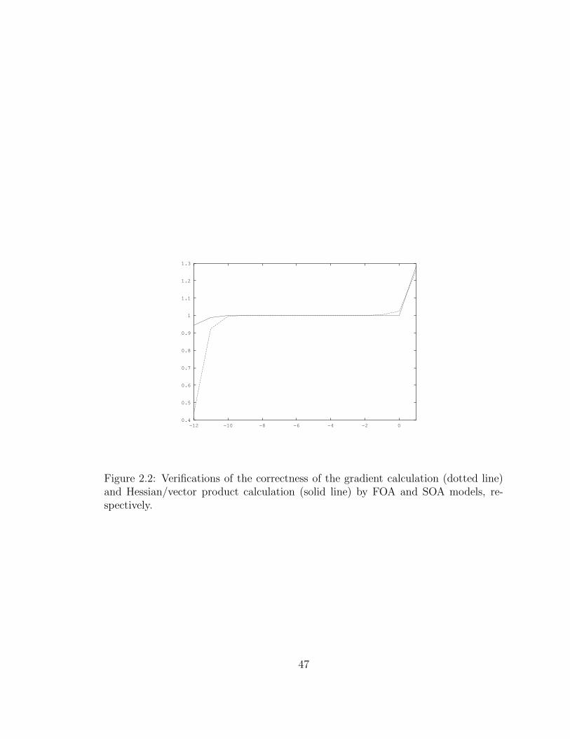
0.4
0.5
0.6
0.7
0.8
0.9
1
1.1
1.2
1.3
-12 -10 -8 -6 -4 -2 0
Figure 2.2: Verifications of the correctness of the gradient calculation (dotted line)and Hessian/vector product calculation (solid line) by FOA and SOA models, re-spectively.
47
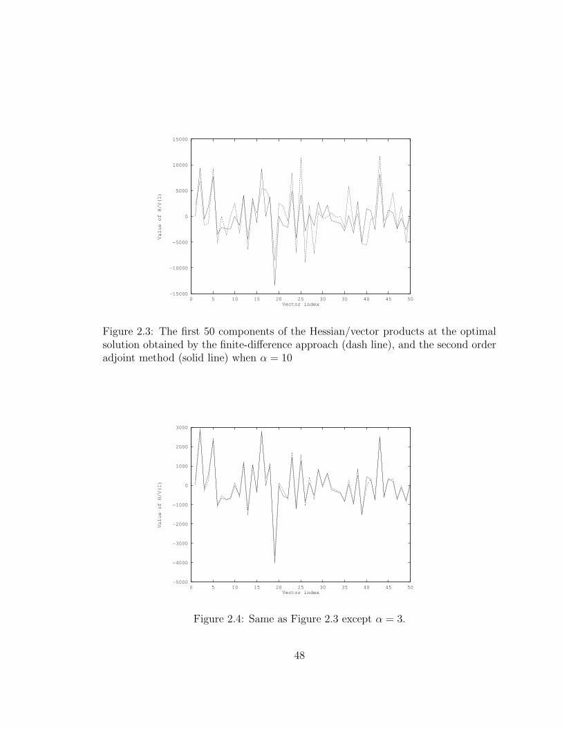
-15000
-10000
-5000
0
5000
10000
15000
0 5 10 15 20 25 30 35 40 45 50
Value of H/V(I)
Vector index
Figure 2.3: The first 50 components of the Hessian/vector products at the optimalsolution obtained by the finite-difference approach (dash line), and the second orderadjoint method (solid line) when α = 10
-5000
-4000
-3000
-2000
-1000
0
1000
2000
3000
0 5 10 15 20 25 30 35 40 45 50
Value of H/V(I)
Vector index
Figure 2.4: Same as Figure 2.3 except α = 3.
48
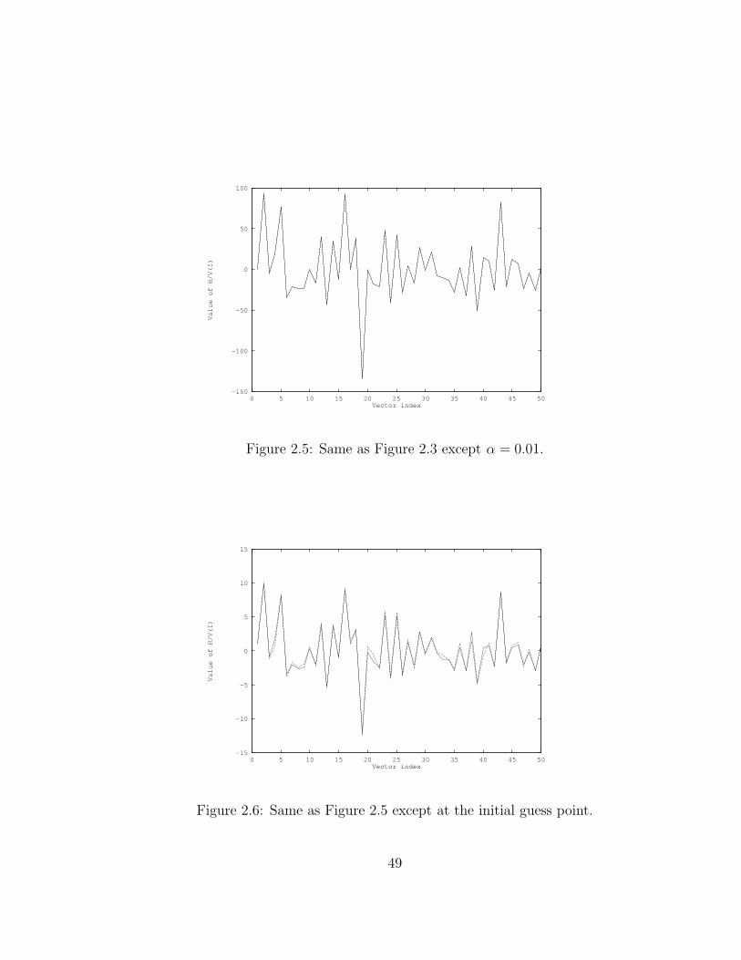
-150
-100
-50
0
50
100
0 5 10 15 20 25 30 35 40 45 50
Value of H/V(I)
Vector index
Figure 2.5: Same as Figure 2.3 except α = 0.01.
-15
-10
-5
0
5
10
15
0 5 10 15 20 25 30 35 40 45 50
Value of H/V(I)
Vector index
Figure 2.6: Same as Figure 2.5 except at the initial guess point.
49
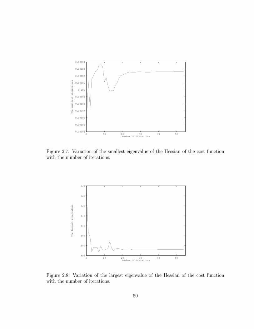
0.00594
0.00595
0.00596
0.00597
0.00598
0.00599
0.006
0.00601
0.00602
0.00603
0.00604
0 10 20 30 40 50
The smallest eigenvalues
Number of iterations
Figure 2.7: Variation of the smallest eigenvalue of the Hessian of the cost functionwith the number of iterations.
495
500
505
510
515
520
525
530
0 10 20 30 40 50
The largest eigenvalues
Number of iterations
Figure 2.8: Variation of the largest eigenvalue of the Hessian of the cost functionwith the number of iterations.
50
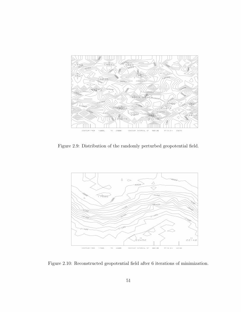
Figure 2.9: Distribution of the randomly perturbed geopotential field.
Figure 2.10: Reconstructed geopotential field after 6 iterations of minimization.
51
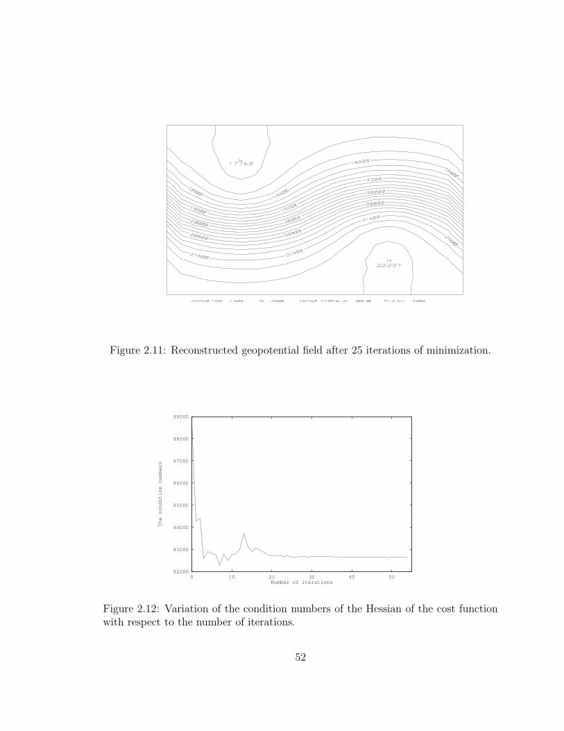
Figure 2.11: Reconstructed geopotential field after 25 iterations of minimization.
82000
83000
84000
85000
86000
87000
88000
89000
0 10 20 30 40 50
The condition numbers
Number of iterations
Figure 2.12: Variation of the condition numbers of the Hessian of the cost functionwith respect to the number of iterations.
52
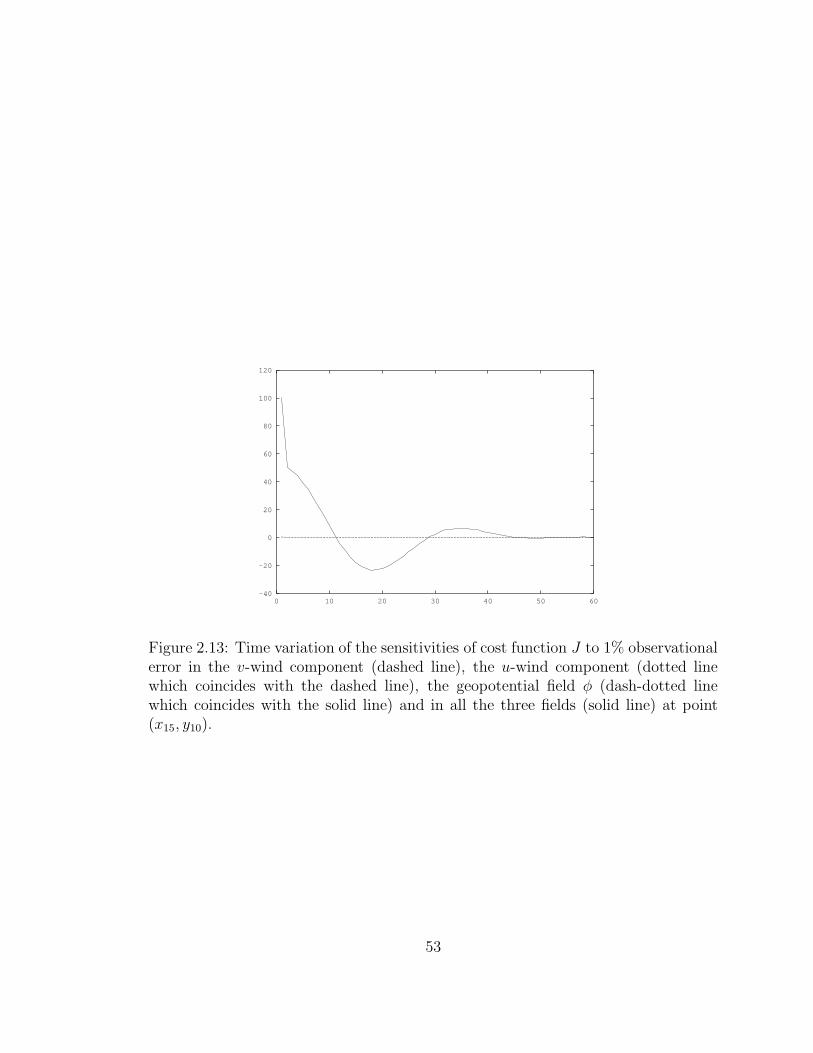
-40
-20
0
20
40
60
80
100
120
0 10 20 30 40 50 60
Figure 2.13: Time variation of the sensitivities of cost function J to 1% observationalerror in the v-wind component (dashed line), the u-wind component (dotted linewhich coincides with the dashed line), the geopotential field φ (dash-dotted linewhich coincides with the solid line) and in all the three fields (solid line) at point(x15, y10).
53
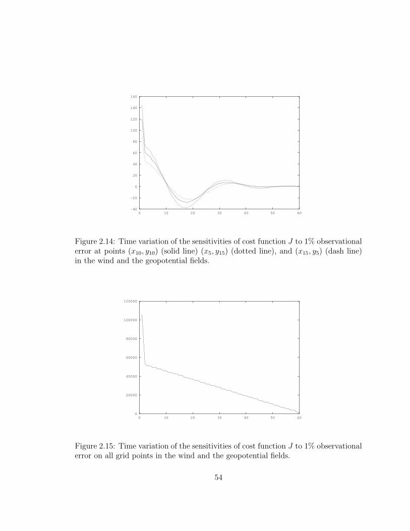
-40
-20
0
20
40
60
80
100
120
140
160
0 10 20 30 40 50 60
Figure 2.14: Time variation of the sensitivities of cost function J to 1% observationalerror at points (x10, y10) (solid line) (x5, y15) (dotted line), and (x15, y5) (dash line)in the wind and the geopotential fields.
0
20000
40000
60000
80000
100000
120000
0 10 20 30 40 50 60
Figure 2.15: Time variation of the sensitivities of cost function J to 1% observationalerror on all grid points in the wind and the geopotential fields.
54
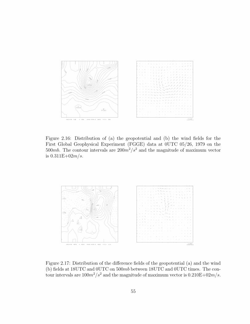
Figure 2.16: Distribution of (a) the geopotential and (b) the wind fields for theFirst Global Geophysical Experiment (FGGE) data at 0UTC 05/26, 1979 on the500mb. The contour intervals are 200m2/s2 and the magnitude of maximum vectoris 0.311E+02m/s.
Figure 2.17: Distribution of the difference fields of the geopotential (a) and the wind(b) fields at 18UTC and 0UTC on 500mb between 18UTC and 0UTC times. The con-tour intervals are 100m2/s2 and the magnitude of maximum vector is 0.210E+02m/s.
55
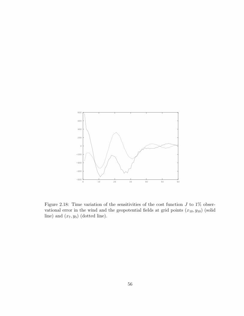
-800
-600
-400
-200
0
200
400
600
800
0 10 20 30 40 50 60
Figure 2.18: Time variation of the sensitivities of the cost function J to 1% obser-vational error in the wind and the geopotential fields at grid points (x10, y10) (solidline) and (x7, y5) (dotted line).
56
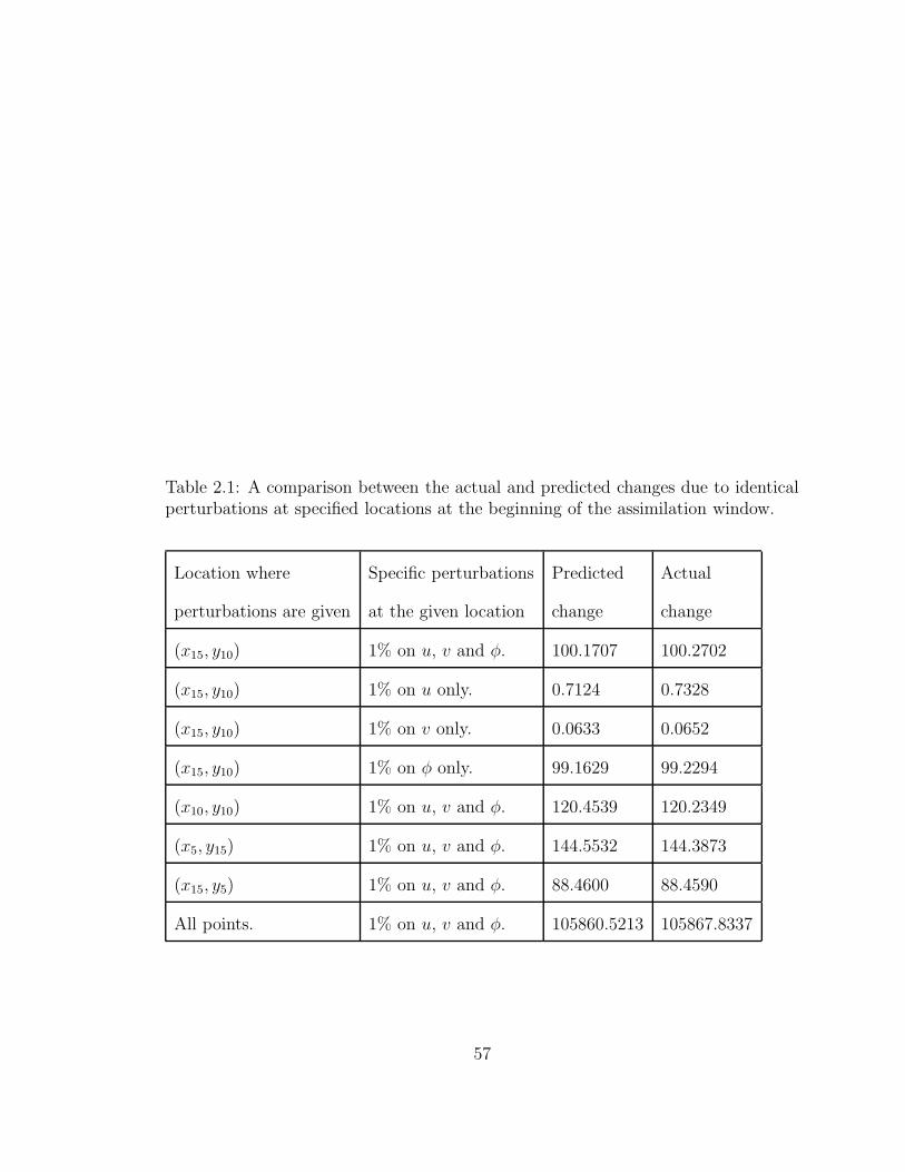
Table 2.1: A comparison between the actual and predicted changes due to identicalperturbations at specified locations at the beginning of the assimilation window.
Location where Specific perturbations Predicted Actual
perturbations are given at the given location change change
(x15, y10) 1% on u, v and φ. 100.1707 100.2702
(x15, y10) 1% on u only. 0.7124 0.7328
(x15, y10) 1% on v only. 0.0633 0.0652
(x15, y10) 1% on φ only. 99.1629 99.2294
(x10, y10) 1% on u, v and φ. 120.4539 120.2349
(x5, y15) 1% on u, v and φ. 144.5532 144.3873
(x15, y5) 1% on u, v and φ. 88.4600 88.4590
All points. 1% on u, v and φ. 105860.5213 105867.8337
57
CHAPTER 3
THE ADJOINT TRUNCATED NEWTON ALGORITHM FOR
LARGE-SCALE UNCONSTRAINED OPTIMIZATION
3.1 Introduction
The issue of variational 4-dimensional data assimilation (VDA) applied to the
shallow water equations (SWE) model has been the subject of several recent re-
search papers such as [34], [108], [218], [225], [227], [228] etc. In Chapter 2, we
introduced the SOA theory and applied it the SWE model. It was found that the
Hessian/vector product obtained by using the SOA approach is more accurate than
the finite difference approach and the convergence rate is slow.
Newton descent methods have never been used in a realistic large-scale optimal
control of distributed parameters problems due to the fact that computation and
storage of the Hessian matrix are too costly to be practical. Among feasible methods
for large-scale unconstrained minimization are (a) the limited memory conjugate
gradient method ([144], [190]); (b) quasi-Newton type algorithms ([46], [70], [155]);
(c) limited-memory quasi-Newton methods such as LBFGS algorithm ([117], [154])
and (d) truncated-Newton algorithms ([49, 131, 133, 134, 137, 185, 186]).
The TN algorithm can be applied to many problems such as to the above uncon-
strained minimization problem (Eq. (2.1)) and to parallel minimization problems
([135], [136]). The main purpose of the present work is to propose a modified version
of the truncated-Newton (TN) algorithm of Nash [134] which uses the SOA tech-
nique to obtain a more accurate Hessian/vector product required in calculating the
58
Newton line search direction and to compare the numerical results obtained by the
ATN algorithm with these obtained by the TN algorithm of Nash [134] as well as by
the LBFGS algorithm [117]. The ATN algorithm is only useful for optimal control
problems where adjoint model codes exist or could be easily derived.
The truncated-Newton algorithms attempt to blend the rapid (quadratic) conver-
gence rate of classic Newton method with feasible storage [134] and computational
requirements [137] for large-scale unconstrained minimization problems. When these
algorithms are used for the large-scale unconstrained minimization [227], the Hes-
sian/vector product is usually obtained by applying a finite-difference (FD) approx-
imation technique to the gradient of the cost function with respect to the initial
conditions, while the gradient is calculated by using the first order adjoint (FOA)
technique. Other alternatives for obtaining the Hessian/vector product such as auto-
matic differentiation ([55], [69]), analytical evaluation and higher order FD approxi-
mations exist. However, they are either not feasible for this optimal control problem
applied to VDA or are too costly to apply.
We will introduce in Section 3.2 the FOA and the SOA techniques used in the
VDA to obtain a more accurate Hessian/vector product. In Section 3.3 we present
numerical results obtained by using the ATN algorithm , and compare them with
the results obtained by using the limited memory quasi-Newton algorithm of Liu
and Nocedal [117] and the truncated-Newton algorithm of Nash [134]. A detailed
discussion concerning the accuracy of the FD approximation of the Hessian/vector
product and the sources of error related to this approximation is provided. Conclu-
sions as well as topics for further research related to the ATN approach are presented
in Section 3.4.
59
3.2 The adjoint Newton algorithm
3.2.1 Description of the first and second order adjoint theories
For a perturbation U ′ on the initial condition U in Eq. (1.5), the exact evolution
of the resulting solution due to the initial perturbation U ′ is given by the difference,
~X2 − ~X1, between the two solutions of the model Eq. (1.4) with initial conditions
~X1(t0) = U and ~X2(t0) = U + U ′, respectively. The tangent linear variable defined
by Eqs. (1.10)-(1.11) only yields a second order approximation, with respect to U ′,
to the exact evolution of the perturbation due to this perturbation U ′. The Gateaux
derivative, < ∇UJ, U′ >, of the cost function J is given by
δJ =< ∇UJ, U′ >=
∫ tf
t0
< W (C ~X − ~Xo), CX > dt, (3.1)
To exhibit the linear dependence of δJ with respect to U ′ and consequently in
order to compute the gradient of J , we introduce the adjoint variable P . Taking the
inner product of Eqs. (1.10) with −P and integrating between times t0 and tf gives
∫ ft
t0
< −P, ∂X∂t
> dt =∫ ft
t0
< −P, ∂F∂ ~X
X > dt, (3.2)
Integrating by parts, one obtains
< −P (tf), X(tf) > + < P (t0), X(t0) > +∫ tf
t0
< X,∂P
∂t>
= −∫ tf
t0
< [∂F
∂ ~X]∗P, X > dt, (3.3)
or
< −P (tf ), X(tf ) > + < P (t0), X(t0) >
=∫ tf
t0
< X,−∂P∂t
− [∂F
∂ ~X]∗P > dt, (3.4)
60
Now let us define P as being the solution of
−∂P∂t
=(∂F
∂ ~X
)∗P + C∗W (C ~X − ~Xo), (3.5)
P (tf) = 0, (3.6)
Then from Eq. (3.1) one obtains
δJ(U, U ′) =< ∇UJ, U′ >=< U ′, P (t0) > (3.7)
and
∇UJ = P (t0). (3.8)
Therefore the gradient of the cost function is obtained by a backwards integration
of the adjoint system (3.5-3.6). The dependence of J on the initial condition U is
implicit via X.
It is important to realize that the TLM defined by Eqs. (1.10)-(1.11) is only
second order accurate except when the original model equations Eq. (1.4) are linear.
Although the TLM is used to derive Eq. (3.8), Eq. (3.8) is exact since there is
no TLM variable in the FOA model defined by Eqs. (3.5 and 3.6). This point is
illustrated in Appendix B by using a simple nonlinear model.
For the perturbation U ′ on the initial condition U , the resulting perturbation on
the variable P , P , may be obtained from Eqs. (3.5)–(3.6) as
− ∂P
∂t=
(∂F
∂ ~X
)∗P +
[ ∂2F
∂ ~X2X
]∗P + C∗WCX, (3.9)
P (tf) = 0. (3.10)
Eqs. (3.9) and (3.10) define the SOA model of Eqs. (1.4) and (1.5).
Let us denote the FOA variable after a perturbation U ′ on the initial condition
U by P(U+U ′), then according to the definition
P(U+U ′)(t0) = P (t0) + P (t0). (3.11)
61
Expanding ∇U+U ′J around U in Taylor series and retaining only the first order terms,
results in
∇U+U ′J = ∇UJ + ∇2UJ · U ′ +
1
2(U ′)∗
∂3J(~ξ0)
∂U3U ′, (3.12)
where ∇2UJ is the Hessian matrix of second derivatives of the cost function with
respect to the initial condition and ~ξ0 is a point in the interval [U, U +U ′]. From Eq.
(3.8), we know that
∇U+U ′J = P(U+U ′)(t0). (3.13)
Using Eq. (3.8) and Eqs. (3.11)-(3.12), one obtains
∇2UJ · U ′ = P (t0) −
1
2(U ′)∗
∂3J(~ξ0)
∂U3U ′, (3.14)
where G = ∇2UJ . Therefore the error in a SOA approximation is proportional to
‖U ′‖2.
3.2.2 The adjoint truncated-Newton method.
We provide a brief description of the ATN algorithm which differs from the TN
algorithm ([134], [137]) only in the Hessian/vector calculation required for solving
the Newton equations at the k-th iteration
Gk~dk = −~gk, (3.15)
where Gk is the Hessian of the cost function, ~dk is the linear search direction and
~gk = ∇J(~Uk) is the gradient of the cost function with respect to the initial conditions.
For a complete description of the TN algorithm, see Nash [134] and Appendix C.
The main steps of the ATN algorithm are as follows:
(1) Choose ~U0, an initial guess to the minimizer ~U∗ and set the iteration counter
to k = 0.
62
(2) Test ~Uk for convergence. If the following convergence criterion is satisfied
‖~gk‖ < 10−5 · ‖~g0‖, (3.16)
then stop. Otherwise continue.
(3) Solve approximately the Newton Eqs. (3.15) using a preconditioned
modified-Lanczos algorithm where the Hessian/vector product is obtained
using a backwards integration of of the SOA model given by Eqs. (3.9) and
(3.10).
(4) Set k = k + 1 and update
~Uk+1 = ~Uk + αk~dk, (3.17)
where αk is the step-size obtained by conducting a line search using Davi-
don’s cubic interpolation method [46]. Go to step 2.
The computational cost required to obtain the Hessian/vector product is similar
for both the FD approach and the SOA approach. The SOA approach requires us to
integrate the original nonlinear model and its tangent linear model forward in time
once and integrate the FOA model and the SOA model backwards in time once.
The FD approach requires the integration of the original nonlinear model forward
in time and the FOA model backwards in time twice. The computational costs for
each model integration are comparable.
3.3 Numerical results obtained using the adjoint truncated-Newton
algorithm.
In this section we display numerical results obtained by applying the ATN algo-
rithm for the large-scale unconstrained minimization of the functional in the VDA
63
and compare the results obtained by the ATN algorithm with these obtained by both
the TN and the LBFGS algorithms.
3.3.1 Application of the adjoint truncated-Newton algorithm to varia-
tional data assimilation
A simple experiment was conducted applying the ATN algorithm to minimize
the cost functional J given by Eq. (2.1) in the VDA using the SWE model. The
experiment is devised as follows: the model generated values starting from the ini-
tial condition of Grammeltvedt [75] are used as observations, the initial guess is a
randomly perturbed Grammeltvedt initial condition, and the length of the time as-
similation window is 10 hours. We know the exact solution, i.e. that the value of the
cost function at the minimum must be zero since we must retrieve the original initial
conditions. The ATN algorithm described in Section 3.2.2 is used here for large-scale
unconstrained minimization in the VDA experiment. The maximum number of con-
jugate gradient inner-iterations (MCGI) allowed for each ATN iteration is chosen as
50. The number of BFGS corrections that is to be stored in memory is denoted by
M.
Computations were performed on the CRAY-YMP supercomputer at the Su-
percomputer Computations Research Institute in Florida State University. All the
routines are coded in single precision FORTRAN. The runs were made on the CRAY-
YMP supercomputer, for which the relative machine precision ε is approximately
10−14. The variation of the objective function scaled by its initial value (J/J0) as
well as that of the norm of the gradient also scaled by its initial value (‖~g‖/‖~g0‖)as a function of the number of iterations are displayed in Figure 3.1, respectively.
Figure 3.1 shows that after 16 minimization iterations the value of the cost func-
tion and the norm of the gradient were reduced by 10 and 6 orders of magnitude,
64
respectively. At this stage the prescribed convergence criterion given by Eq. (3.16)
is satisfied. The CPU time used by the ATN algorithm is 10.817s. The rms error,√
‖φr − φu‖2/N , between retrieved geopotential field φr after 16 iterations and the
unperturbed geopotential field φu is 0.9069m2/s2 which is 3 orders of magnitude
smaller than that of the perturbations, where N is the number of components in φr.
We conclude therefore that the ATN algorithm performs well both in terms of CPU
time and the number of iterations.
3.3.2 Numerical results
In this section we compare the numerical behaviour of the ATN unconstrained
minimization algorithm with those of other robust large-scale unconstrained mini-
mization methods. The methods tested are:
(1) TN–the truncated-Newton method of Nash ([132], [134]).
(2) LBFGS–the limited memory quasi-Newton method of Liu and Nocedal [117].
The test problem is the same as that described in section 3.3.1. Computational
efficiency and accuracy were used as leading criteria. For the ATN, TN and LBFGS
algorithms, the same convergence criterion as set by Eq. (3.16) is applied. The
numerical results obtained are displayed in Table 3.1.
The first column displays the unconstrained minimization algorithms tested. The
second column displays the parameters used for each algorithm. The third, fourth
and eighth columns record the number of iterations (Iter.), the number of function
calls (NFC), and the CPU time in seconds required to satisfy prescribed convergence
criteria, respectively. The fifth column records the total number of conjugate gra-
dient iterations (NCG) used to determine the Newton descent directions. The next
two columns display the scaled cost function (Jk/J0) and the scaled gradient norm
(‖~gk‖/‖~g0‖) at the end of the assimilation process, respectively.
65
Both the ATN and TN algorithms obtain the Newton descent direction by solving
approximately the Newton equations using a truncated conjugate gradient algorithm.
They only differ in the calculation of the Hessian/vector product. However their
relative performances turn out to be dramatically different. Table 3.1 indicates that
for different MCGI allowed for each inner iteration, the ATN algorithm outperforms
the TN algorithm. When MCGI is 5, the TN algorithm stopped without satisfying
the prescribed convergence criterion. When MCGI is 4, the TN algorithm required
three times the CPU time used by the ATN algorithm to satisfy the same convergence
criteria. In terms of CPU times the ATN, TN and LBFGS algorithms yield optimal
results when MCGI is 4 and 3 and M is 5, respectively. In this case the CPU time
required by ATN algorithm is about half of that required by either the TN or the
LBFGS algorithms.
If we relax the convergence criterion given by Eq. (3.16) by two orders of mag-
nitude, then the ATN, TN and LBFGS algorithms require 8, 16 and 55 iterations
and take 5s, 8s and 6s of CPU time to converge where we used MCGI=50 for the
ATN and TN and M=5 for the LBFGS, respectively. Therefore even for the relaxed
accuracy requirement the ATN algorithm performed slightly better than the LBFGS
algorithm in terms of CPU time required to satisfy the convergence criteria.
Let us define the degree of nonlinearity of the cost function at ~U as
DN(~U) = (J(~U) − [J(~U∗) + pt∇J(~U∗) + 0.5pt∇2J(~U∗)p])/‖p‖3, (3.18)
where ~U is a point between the starting point U0 and the solution ~U∗, p = ~U − ~U∗
and pt denotes the transpose of p. DN(~U) gives a measure of the size of the third
derivative or a deviation from quadratic behaviour (see Nash and Nocedal [137]).
For our test problem we noticed that DN(~U) increases from 1.7E−7 to 4.7E+12
as ~U approaches ~U∗ from the starting point. Therefore we may classify our test prob-
lem as a highly nonlinear problem near the solution. Then it is not surprising that
66
the LBFGS algorithm outperforms the TN algorithm in terms of CPU time (Ta-
ble 3.1) if we take into account Nash’s observation that for most of highly nonlinear
problems, the LBFGS algorithm performs better than the TN algorithm [134]. Our
point is that even in this case, if we use a more accurate line search direction in the
TN algorithm, the TN can outperform the LBFGS as the ATN does for the particular
optimal control problem tested here.
Therefore we conclude that the ATN algorithm turns out to be the most accurate
and robust amongst the large-scale unconstrained minimization algorithms tested in
terms of both CPU time and number of iterations for the specific problem tested here.
3.3.3 An accuracy analysis of the Hessian/vector product.
The Hessian/vector product GkU′ for a given U ′ required by the inner conjugate
algorithm of the ATN algorithm is obtained by the SOA technique where the vector
U ′ serves as the initial condition for the TLM model. The Hessian/vector product
GkU′ of the TN algorithm is obtained by the following FD approximation GkU
′|FD
GkU′|FD =
g(~Uk + hU ′) − g(~Uk)
h, (3.19)
where Gk is the Hessian matrix at the k-th outer iteration, h =√
ε× (1 + ‖~Uk‖) is
the differencing parameter, where ε is taken to be the machine precision [134], and
the computed gradients g(~Uk + hU ′) and g(~Uk) are obtained by using Eq. (3.8).
In order to consider the accuracy of the FD approximation with respect to the
differencing parameter h, we assume h ∈ [hmin, hmax] where hmin and hmax are taken
to be the machine accuracy ε and 103, respectively, such that the interval [hmin, hmax]
contains all reasonable sequences of differencing parameters.
Although a FOA integration yields an exact gradient of the cost function with
respect to the control variables, when a computer is used to calculate the gradient
67
there is always computational errors involved. Let a positive quantity ε0 denote an
error bound on the absolute error in the computed gradients of the cost function using
Eq. (3.8) at ~Uk and ~Uk + hU ′. It will be assumed throughout this chapter that the
value of ε at the given point is available; an effective technique for computing ε is
given by Hamming [82].
So one has
gt(~Uk) = ~g(~Uk) + θ0ε0, (3.20)
gt(~Uk + hU ′) = ~g(~Uk + hU ′) + θ1ε0, (3.21)
where |θ0| ≤ 1 and |θ1| ≤ 1. Using a Taylor series expansion, one obtains
~g(~Uk + hU ′) = ~g(~Uk) + h∂~g(~Uk)
∂~Uk
U ′ +h2
2(U ′)∗
∂2~g(~Uk)
∂~U2k
U ′ + · · ·
= ~g(~Uk) + hGkU′|t +
h2
2(U ′)∗
∂2~g(~ξ)
∂~U2k
U ′, (3.22)
where GkU′|t = [∂~g(~Uk)/∂~Uk]U
′ denotes the true value of the Hessian/vector product
and ~ξ is a point in the interval [~Uk, ~Uk + hU ′].
Solving for GkU′|t from Eq. (3.22) and using Eqs. (3.21) and (3.20), one obtains
GkU′|t =
~g(~Uk + hU ′) − ~g(~Uk)
h− h
2(U ′)∗
∂2~g(~ξ)
∂~U2k
U ′
=g(~Uk + hU ′) − g(~Uk)
h+
(θ0 − θ1)ε0h
− h
2(U ′)∗
∂2~g(~ξ)
∂~U2k
U ′, (3.23)
where −h(U ′)∗[∂2~g(~ξ)/∂~U2k ]U ′/2 is the truncation error and (θ1 − θ0)ε0/h is the con-
dition error [70]. Combining Eqs. (3.19) and (3.23), one obtains
GkU′|t = GkU
′|FD +(θ0 − θ1)ε0
h− h
2(U ′)∗
∂2~g(~ξ)
∂~U2k
U ′. (3.24)
According to Eq. (3.14)
GkU′|t = GkU
′|SOA − 1
2(U ′)∗
∂3J(~ξ0)
∂U3k
U ′, (3.25)
68
where GkU′|SOA denotes the Hessian/vector product obtained by using the SOA tech-
nique. Since GkU′|t and ∂3J(~ξ0)/∂U
3k are not available, one can not calculate the over
all errors in both SOA and finite-difference approximations. However one may inves-
tigate the truncation and condition errors by looking at the difference between the
GkU′|SOA and GkU
′|FD,
GkU′|SOA −GkU
′|FD =
+(θ0 − θ1)ε0
h− h
2(U ′)∗
∂2~g(~ξ)
∂~U2k
U ′ 1
2(U ′)∗
∂3J(~ξ0)
∂U3k
U ′, (3.26)
where the error U ′(U ′)∗[∂3J(~ξ0)/∂U3k ]U ′/2 resulting from the SOA approximation is
fixed for fixed U ′ while the truncation and condition errors resulting from the finite-
difference approximation change with differencing parameter.
The rms errors between the the Hessian/vector products obtained by using the
SOA and the FD techniques with various differencing parameters are displayed in
Table 3.2. This Table indicates that (a) the Hessian/vector products obtained by
the FD and the SOA techniques follow a relationship given by Eq. (3.26) where
the error term O(h) dominates for large differencing parameter h, (b) for a small
differencing parameter, the error term O(1/h) in Eq. (3.26) dominates. The FD
technique involves subtractions of nearly equal numbers which result in cancellations
of significant digits and which are the reason for the increase in the rms errors and
(c) the differencing parameter h in the TN Nash [134] may become too small near the
end of the minimization process. Thus in practice, the SOA approximation is more
accurate than the finite-difference approximation in calculating the Hessian/vector
product.
Figure 3.2 shows the first 50 components of the scaled difference between the Hes-
sian/vector products obtained by using the SOA and the FD techniques respectively
after 15 iterations using the ATN algorithm. The differencing parameter is chosen
as h1 = h (solid line), h2 = h × 10−1 (dotted line) and h3 = h × 103 (dashed line)
69
where h is the differencing parameter used in the original TN Nash [134] minimiza-
tion algorithm, respectively. The results with h3 = h × 103 clearly illustrate that
toward the end of the minimization the differencing parameter in the TN Nash [134]
is too small. This result agrees with the rms error evolution in Table 3.2. It can be
seen that the FD technique can yield an approximation of similar accuracy to that
obtained by SOA technique if the differencing parameter is properly chosen. However
simply increasing or decreasing the differencing parameter h at every iteration will
not improve the performance of the TN minimization algorithm since the differencing
parameter depends on the vector U ′ at each iteration and the vector U ′ is not known
prior to performing the minimization iteration.
The differencing parameter h should be chosen such as (a) it balances the trunca-
tion error of the order h with the condition error ([70], [72], [74]) of order 1/h, (b) h
must be adjusted to the size of vector U ′ [185, 186] and (c) h should not become so
small as to cause cancellations of significant digits [198]. It is difficult to choose an h
which satisfies all these requirements. Some good choices of h in addition to that used
in the TN Nash minimization algorithm [134] are h = 2(1 + ‖~Uk‖)√ε/‖U ′‖ [185, 186],
h =√ε/‖U ′‖ [49] and h = 2(1 + ‖~Uk‖)
√ε/‖U ′‖2 [155] etc. But results (not shown
here) obtained using these choices of h are no better than those obtained when
h =√
ε× (1 + ‖~Uk‖) as used in the TN Nash [134]. All these choices of h cause
cancellations of significant digits at some stage of the minimization process.
The convergence rate of the ATN minimization algorithm is best understood intu-
itively by splitting the error into three terms [155]. Let ~U∗ be the true solution to the
problem, G(~Uk) the exact Hessian at ~Uk, Gk the approximate Hessian obtained by the
FD or by the SOA technique, and Hk the approximate matrix to the inverse Hessian
matrix that the inner conjugate gradient algorithm actually used, i.e. ~pk = −Hk~gk.
Then, if the step size chosen was 1 and if G(~Uk) is positive definite,
~Uk+1 − ~U∗ = ~Uk −Hk~gk − ~U∗
70
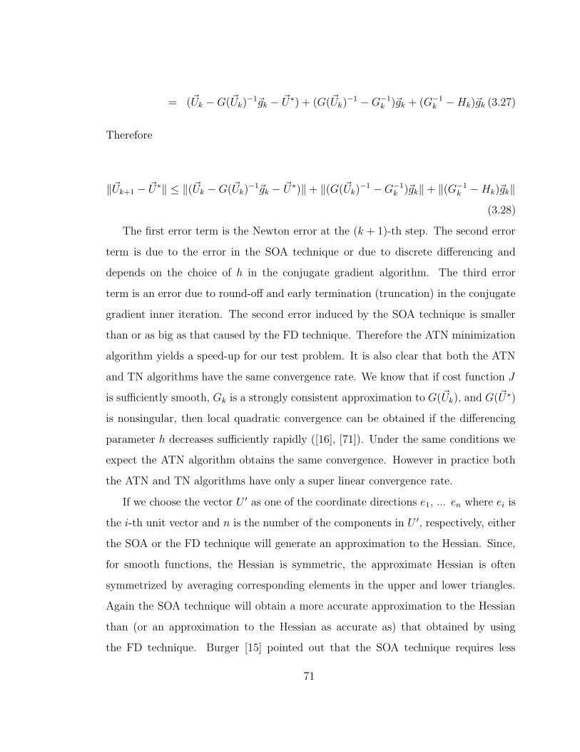
= (~Uk −G(~Uk)−1~gk − ~U∗) + (G(~Uk)
−1 −G−1k )~gk + (G−1
k −Hk)~gk (3.27)
Therefore
‖~Uk+1 − ~U∗‖ ≤ ‖(~Uk −G(~Uk)−1~gk − ~U∗)‖ + ‖(G(~Uk)
−1 −G−1k )~gk‖ + ‖(G−1
k −Hk)~gk‖(3.28)
The first error term is the Newton error at the (k + 1)-th step. The second error
term is due to the error in the SOA technique or due to discrete differencing and
depends on the choice of h in the conjugate gradient algorithm. The third error
term is an error due to round-off and early termination (truncation) in the conjugate
gradient inner iteration. The second error induced by the SOA technique is smaller
than or as big as that caused by the FD technique. Therefore the ATN minimization
algorithm yields a speed-up for our test problem. It is also clear that both the ATN
and TN algorithms have the same convergence rate. We know that if cost function J
is sufficiently smooth, Gk is a strongly consistent approximation to G(~Uk), and G(~U∗)
is nonsingular, then local quadratic convergence can be obtained if the differencing
parameter h decreases sufficiently rapidly ([16], [71]). Under the same conditions we
expect the ATN algorithm obtains the same convergence. However in practice both
the ATN and TN algorithms have only a super linear convergence rate.
If we choose the vector U ′ as one of the coordinate directions e1, ... en where ei is
the i-th unit vector and n is the number of the components in U ′, respectively, either
the SOA or the FD technique will generate an approximation to the Hessian. Since,
for smooth functions, the Hessian is symmetric, the approximate Hessian is often
symmetrized by averaging corresponding elements in the upper and lower triangles.
Again the SOA technique will obtain a more accurate approximation to the Hessian
than (or an approximation to the Hessian as accurate as) that obtained by using
the FD technique. Burger [15] pointed out that the SOA technique requires less
71
computing time than direct differentiation in obtaining the approximate Hessian and
thus the results from the former method are more accurate than these from the latter
method. Our results are consistent with those of Burger [15] in as far as the aspect of
accuracy is concerned. Similar results to ours were obtained by Symes [201] showing
the advantage of using the SOA technique to obtain the Hessian/vector product in
the TN algorithm.
In summary, we conclude that the SOA technique yields a more accurate value
of the Hessian/vector product compared to the FD technique for optimal control
problems tested here. When the differencing parameter h is too small or too big,
cancellations of significant digits or truncation errors dominate the FD approximation.
It is hard to avoid the occurrence of these two types of error in the minimization
process when the FD technique is used [211]. Use of more accurate Hessian/vector
products in the inner conjugate gradient iteration of the TN algorithm results in
a better line search direction as measured by the amount of decrease in the cost
function, but not in the residuals [138].
3.4 Conclusions
In this chapter, we proposed a modified version of the Nash truncated-Newton
algorithm [138] by using the FOA and the SOA techniques, i.e. we proposed a new
method to obtain a Hessian/vector product to be used in the process of solving the
Newton equations for the TN minimization algorithm for an optimal control problem.
The costs of the SOA approach and the FD approach are computationally compa-
rable, each of them requiring four different model integrations when applied to the
optimal control problem tested here. But the former approach yields a more accurate
Hessian/vector product, while the latter provides only a less accurate approxima-
tion to the Hessian/vector product if the finite-differencing parameter is taken to be
72
the square root of the machine accuracy. The numerical results indicate that the
new Hessian/vector calculation strategy employed in the modified-Lanczos algorithm
of Nash [138] allows the ATN algorithm to perform better than either the TN or
the LBFGS algorithms both in terms of CPU time as well as in term of number of
iterations required to satisfy the prescribed convergence criterion in our test prob-
lems. This result may be very useful, since truncated-Newton type methods and
conjugate-gradient methods have comparable storage requirements and constitute
the only practical methods for solving many large-scale unconstrained minimization
problems arising in 4-D VDA.
In our test example, the eigenvalues of the Hessian at each iteration are posi-
tive [218], which implies the Hessians are positive definite and the cost function is
strictly convex. Therefore the existence of a local minimum is assured. However the
condition numbers at each iteration are large [218], which explains why all three algo-
rithms require more than 16 iterations to satisfy the prescribed convergence criteria.
Theoretically, the TN and the ATN minimization algorithms have the same con-
vergence rate. However the ATN algorithm results in a speed-up due to the use of a
more accurate Hessian/vector product to obtain the line search direction.
The ATN algorithm, like its TN counterpart, is a close approximation to the
Newton method at reasonable storage and computational cost. We expect the ATN
algorithm to yield a similar speed-up for other large-scale unconstrained minimiza-
tion problems related to optimal control and VDA. The idea of obtaining the Hes-
sian/vector product using the SOA technique can be applied in other settings requir-
ing large-scale minimization, in cases where an adjoint model formulation is possible,
or via automatic differentiation techniques [77] - pointing to a more general applica-
bility of this idea. An application of the ATN minimization algorithm for minimizing
a cost functional in optimal control of distributed parameters in a primitive equations
73

3-D spectral model will be reported separately, once the SOA model of this model is
derived.
74
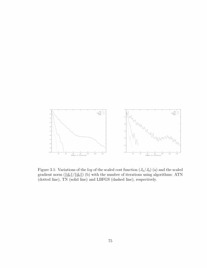
-10
-9
-8
-7
-6
-5
-4
-3
-2
-1
0
20 40 60 80 100 120 140Number of Iterations
’TN’’LBFGS’’ATN’
-6
-5
-4
-3
-2
-1
0
20 40 60 80 100 120 140Number of Iterations
’TN’’LBFGS’’ATN’
Figure 3.1: Variations of the log of the scaled cost function (Jk/J0) (a) and the scaledgradient norm (‖~gk‖/‖~g0‖) (b) with the number of iterations using algorithms: ATN(dotted line), TN (solid line) and LBFGS (dashed line), respectively.
75
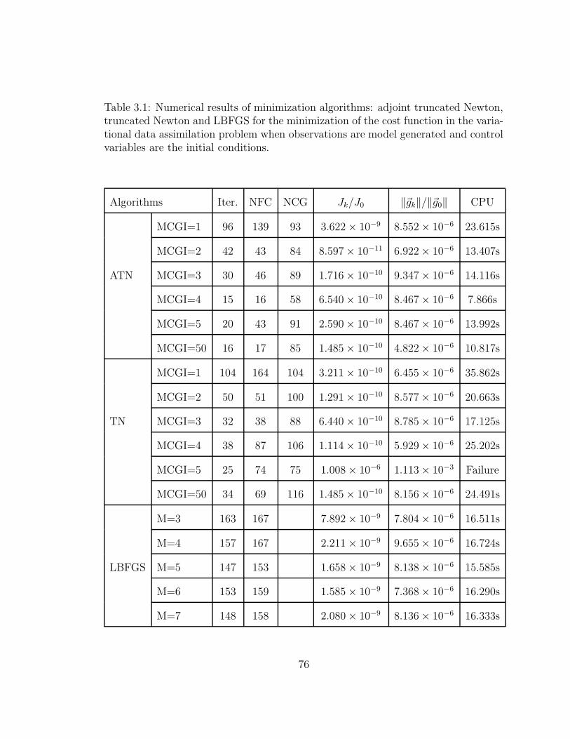
Table 3.1: Numerical results of minimization algorithms: adjoint truncated Newton,truncated Newton and LBFGS for the minimization of the cost function in the varia-tional data assimilation problem when observations are model generated and controlvariables are the initial conditions.
Algorithms Iter. NFC NCG Jk/J0 ‖~gk‖/‖~g0‖ CPU
MCGI=1 96 139 93 3.622 × 10⁻⁹ 8.552 × 10⁻⁶ 23.615s
MCGI=2 42 43 84 8.597 × 10⁻¹¹ 6.922 × 10⁻⁶ 13.407s
ATN MCGI=3 30 46 89 1.716 × 10⁻¹⁰ 9.347 × 10⁻⁶ 14.116s
MCGI=4 15 16 58 6.540 × 10⁻¹⁰ 8.467 × 10⁻⁶ 7.866s
MCGI=5 20 43 91 2.590 × 10⁻¹⁰ 8.467 × 10⁻⁶ 13.992s
MCGI=50 16 17 85 1.485 × 10⁻¹⁰ 4.822 × 10⁻⁶ 10.817s
MCGI=1 104 164 104 3.211 × 10⁻¹⁰ 6.455 × 10⁻⁶ 35.862s
MCGI=2 50 51 100 1.291 × 10⁻¹⁰ 8.577 × 10⁻⁶ 20.663s
TN MCGI=3 32 38 88 6.440 × 10⁻¹⁰ 8.785 × 10⁻⁶ 17.125s
MCGI=4 38 87 106 1.114 × 10⁻¹⁰ 5.929 × 10⁻⁶ 25.202s
MCGI=5 25 74 75 1.008 × 10⁻⁶ 1.113 × 10⁻³ Failure
MCGI=50 34 69 116 1.485 × 10⁻¹⁰ 8.156 × 10⁻⁶ 24.491s
M=3 163 167 7.892 × 10⁻⁹ 7.804 × 10⁻⁶ 16.511s
M=4 157 167 2.211 × 10⁻⁹ 9.655 × 10⁻⁶ 16.724s
LBFGS M=5 147 153 1.658 × 10⁻⁹ 8.138 × 10⁻⁶ 15.585s
M=6 153 159 1.585 × 10⁻⁹ 7.368 × 10⁻⁶ 16.290s
M=7 148 158 2.080 × 10⁻⁹ 8.136 × 10⁻⁶ 16.333s
76
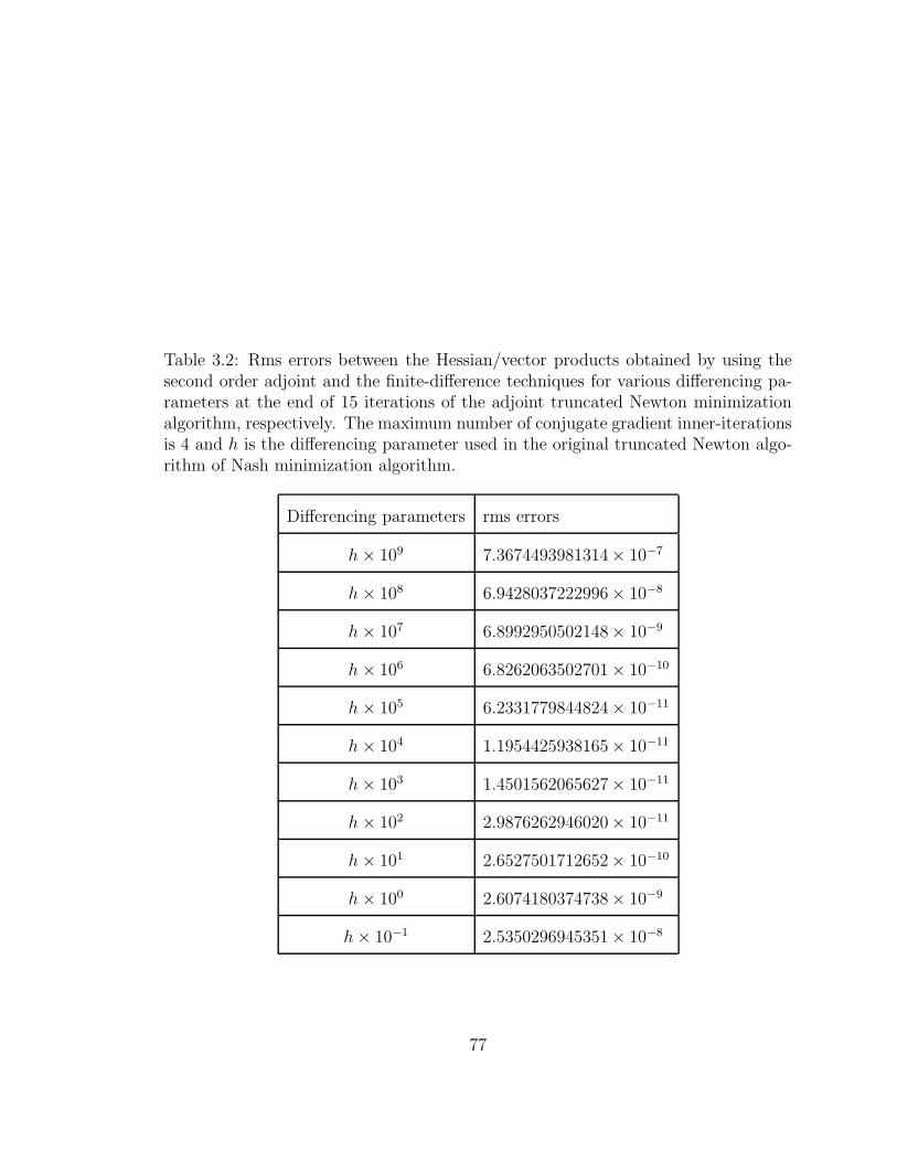
Table 3.2: Rms errors between the Hessian/vector products obtained by using thesecond order adjoint and the finite-difference techniques for various differencing pa-rameters at the end of 15 iterations of the adjoint truncated Newton minimizationalgorithm, respectively. The maximum number of conjugate gradient inner-iterationsis 4 and h is the differencing parameter used in the original truncated Newton algo-rithm of Nash minimization algorithm.
Differencing parameters rms errors
h× 109 7.3674493981314× 10−7
h× 108 6.9428037222996× 10−8
h× 107 6.8992950502148× 10−9
h× 106 6.8262063502701× 10−10
h× 105 6.2331779844824× 10−11
h× 104 1.1954425938165× 10−11
h× 103 1.4501562065627× 10−11
h× 102 2.9876262946020× 10−11
h× 101 2.6527501712652× 10−10
h× 100 2.6074180374738× 10−9
h× 10−1 2.5350296945351× 10⁻⁸
77
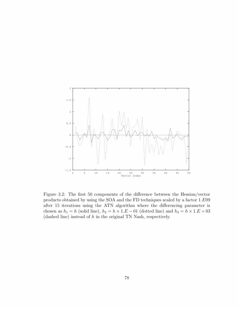
-1.5
-1
-0.5
0
0.5
1
1.5
2
0 5 10 15 20 25 30 35 40 45 50Vector index
Figure 3.2: The first 50 components of the difference between the Hessian/vectorproducts obtained by using the SOA and the FD techniques scaled by a factor 1.E09after 15 iterations using the ATN algorithm where the differencing parameter ischosen as h1 = h (solid line), h2 = h× 1.E − 01 (dotted line) and h3 = h× 1.E + 03(dashed line) instead of h in the original TN Nash, respectively.
78
CHAPTER 4
THE FSU GLOBAL SPECTRAL MODEL
4.1 Introduction
The spectral method is a popular technique for hemispheric or global atmospheric
modeling, in both operational and research applications. This has largely been a
consequence of the discovery of the transform technique, developed by Orszag [156],
and later refined by Bourke [12]. There are a number of advantages which bespeak
the superiority of the spectral method over the grid-point method for large-scale
prediction models. In the first place, the spectral coefficient representation of the
dependent atmospheric variables carries more information (i.e. smaller scales) than
the grid-point depiction, for an equal number of degree of freedom. Moreover, the
Galerkin procedure (used in most of spectral models), by definition, assures that
when nonlinear terms are evaluated there is no aliasing of unresolved scales into those
scales which are resolved by the model’s truncation limit. Aliasing is a common cause
of nonlinear instability and phase errors in grid-point models, even for those using
fairly sophisticated finite difference approximations for the nonlinear advective terms.
With the aid of transform technique, the spectral model can efficiently compute the
nonlinear terms by forming products in the real (grid) space and transforming them
back to the spectral (coefficients) space. The essence of the Galerkin procedure will
be preserved if exact numerical quadrature is employed for the transforms. Prior
to the introduction of the transform technique, it was thought necessary to remain
in the spectral space and to compute and store a tremendous number of interaction
coefficients (arising from the nonlinearities in the governing equations) in the course
79
of a numerical forecast. The removal of this encumbrance has made spectral models
competitive, in terms of computational overhead, with respect to their grid-point
counterparts.
An added advantage which arises from the transform procedure is seen when phys-
ical effects are to be incorporated into the prediction scheme. The availability of the
dependent variables at the transform grid points enables the calculations of parame-
terized physical effects in the real space. These may then be added to the dynamic
tendencies prior to transforming back to the spectral domain. Drawbacks of the spec-
tral method are related to computational issues which may become a problem for high
resolution spectral methods, specially related to the unavailability of fast Legendre
transforms. Moreover transporting spectral methods to high performance parallel
computers of multiple instruction multiple data type (MIMD) may be less efficient
than the corresponding procedure for finite difference or finite element methods.
The FSUGSM has been developed from the Canadian spectral model of the
Recherche en Prevision Numerique [40]. In the development of the FSUGSM from
the Canadian model, the primary effort has been directed at improving the physical
effect parameterizations, adapting the model code to run efficiently on the NCAR
Cray-1 computer and developing post-forecast diagnostics [162].
The FSUGSM is a multi-level primitive equations model with λ (longitude), θ
(latitude) as horizontal coordinates in the real space and σ
σ =p
ps
, (4.1)
where p and ps are pressure and surface pressure, respectively, as vertical coordinate.
In the horizontal direction, all dependent variables are expanded in a truncated series
of spherical harmonic functions Y ml (λ, θ). Here Y m
l (λ, θ) = Xml (sin θ)eimλ, where
Xml (θ) are the associated Legendre functions of the first kind of order m and degree
l (m is the zonal wave number and m − l is the number of meridional nodes from
80
pole to pole). For real to spectral space transform, any variable, say f(λ, θ, σ, t), is
assumed to be expanded in a truncated series of spherical harmonics
f(λ, θ, σ, t) =J
∑
m=−J
|m|+J∑
l=|m|
fml (σ, t)Y m
l (λ, θ), (4.2)
if rhomboidal truncation is used or
f(λ, θ, σ, t) =J
∑
m=−J
J∑
l=|m|
fml (σ, t)Y m
l (λ, θ), (4.3)
if triangular truncation is used (all experiments in the following chapters are carried
out using a triangular truncation), where fml (σ, t) is the spectral coefficients and J
denotes the rhomboidal or triangular truncation limit.
The rhomboidal type of truncation is so named because it allows an equal number
of meridional degrees of freedom, J , for each of the J zonal (wavenumber) degrees
of freedom. For triangular truncation all mode would have to satisfy −J ≤ m ≤ J ,
l ≤ J . There are several advantages to the triangular truncation, particularly in the
calculation of energetics and energy spectra. However, the superiority of triangular
truncation with respect to the integration of a complicated numerical model has
never been demonstrated. Moreover, the rhomboidal truncation is much simpler to
code, particularly if it is desired to take full advantage of symmetry in integrating a
hemispheric model.
Spectral harmonics are orthogonal, with the normalization constant being incor-
porated into the Legendre functions such that (for arbitrary zonal wave numbers m,
n and meridional indices l, j):
1
2π
∫ π2
−π2
∫ 2π
0Y m
l (λ, θ)(Y nj (λ, θ))t cos θdλdθ = δj
l δnm, (4.4)
where (Y nj (λ, θ))t = (−1)nY −n
j is the complex conjugate of Y nj (λ, θ) and δj
l , δnm are
Kronecker deltas. By choosing our spectral expansion functions to be orthogonal,
we greatly simplify the application of the Galerkin weighted residual procedure. In
81
principle, one could use any set of expansion functions; the Galerkin procedure only
requires that the residue incurred by the spectral approximation of governing equa-
tions be orthogonal to those of the functions [125].
Given the condition imposed by Eq. (4.4) we can determine the spectral expansion
coefficients fml (σ, t) in (4.2) via
fml (σ, t) =
1
2π
∫ π2
−π2
∫ 2π
0f(λ, θ, σ, t)(Y n
j (λ, θ))t cos θdλdθ. (4.5)
It should be noted that if f(λ, θ, σ, t) is an explicit function of the dependent variables
in the governing equations, then the notation fml is used for the left-hand side of Eq.
(4.5).
4.2 Model equations
It is important to notice that σ = 0 at the top of the atmosphere and σ = 1 is at
the earth’s surface. We will employ the usual boundary conditions σ = 0 at σ = 1
and σ = 0.
It is convenient to define the following operators before developing the governing
equations:
F σ =∫ 1
σFdσ; F =
∫ 1
0Fdσ. (4.6)
The real space forms of the governing equations of the FSUGSM are as follows.
This model uses the differentiated forms of the unfiltered primitive equations of mo-
tion and other model equations are the thermodynamic equation, continuity equation,
hydrostatic equation, and a moisture equation, as follows:
Vorticity equation
∂ζ
∂t= −∇ · (ζ + f)~V − ~k · ∇ × (RT∇q + σ
∂~V
∂σ− F ), (4.7)
82
Divergence equation
∂D
∂t= ~k · ∇ × (ζ + f)~V
− ∇ · (RT∇q + σ∂~V
∂σ− F ) −∇2(Φ +
~V · ~V2
), (4.8)
Thermodynamic equation
∂T
∂t= −∇ · ~V T + TD + σγ − RT
Cp
(D +∂σ
∂σ) +HT , (4.9)
Surface pressure tendency equation
∂q
∂t= −D − ∂σ
∂σ− ~V · ∇q, (4.10)
Hydrostatic equation
σ∂Φ
∂σ= −RT, (4.11)
and Moisture equation
∂S
∂t= −∇ · ~V S + SD − σ
∂S
∂σ+HT −HM
− [RT
Cp
− RT 2d
εL(Td)][D +
∂σ
∂σ− σ
σ], (4.12)
where
ζ = vertical component of vorticity = ~k · ∇ × ~V ,
f =Coriolis parameter,
~V= horizontal vector wind,
D = horizontal divergence =∇ · ~V ,
T = the absolute temperature,
q = ln ps,
γ = static stability = RTCpσ
− ∂T∂σ
,
83
σ= vertical motion in sigma coordinates
=(σ − 1)(D + V · ∇q) + Dσ + V σ · ∇q,
Φ= geopotential height,
F= the horizontal frictional force per unit mass,
HT =the diabatic heating,
R= the gas constant for dry air,
Cp =the specific heat of dry air at constant pressure,
Td =the dew point temperature,
S = T − Td is the dew point depression,
ε=the ratio of the molecular weight of water vapor
to effective molecular weight of dry air (0.622),
L(Td) =the latent heat of vaporization of water or ice,
HM =represents moisture sources or sinks.
The moisture Eq. (4.12) results from the combination of the thermodynamic Eq.
(4.9) with an expression for the time rate of change of the dewpoint temperature [40].
To facilitate the application of the spectral transforms and the implementation
of the time differencing scheme, some manipulation of the basic Eqs. (4.7) through
(4.12) will be performed. First, let us introduce some notation. For eastward (zonal)
and northward (meridional) wind components u and v, respectively, we define
U = u cos θ/a
V = v cos θ/a, (4.13)
where a is the earth’s radius. With this transformation, the wind components become
true scalars, with no discontinuities at the north or south poles [176]. Also, the
84
horizontal average over a global σ-surface is defined as,
FH(σ, t) =1
4π
∫ π2
−π2
∫ 2π
0F (λ, θ, σ, t) cos θdλdθ, , (4.14)
For implementation of the semi-implicit algorithm (discussed below), the temperature
is expressed as an initial horizontal (global) mean plus a deviation; hence,
T (λ, θ, σ, t) = T ∗(σ, t) + T ′(λ, θ, σ, t), , (4.15)
where T ∗(σ, t) = TH(σ, t) at t = 0. Likewise, we also have for static stability factor
γ = γ∗ + γ′. Furthermore, let us define a horizontal differential operator for two
functions A and B:
α(A,B) =1
cos2 θ[∂A
∂λ+ cos θ
∂B
∂θ]. (4.16)
Now let us expand the governing Eqs. (4.7–4.12) from vector into scalar (spherical
coordinate) form, make use of Eqs. (4.16) and (4.6) and the definitions of U , V , T ∗,
T ′, γ∗ and γ′. With these manipulations, the governing Eqs. (4.7–4.12) become:
∂ζ
∂t= −α(A,B), (4.17)
∂D
∂t= ∇2(Φ +RT ∗q) = α(B,−A) − a2∇2E, (4.18)
∂T
∂t− γ∗σ − RT ∗
Cp
∂q
∂t= −α(UT ′, V T ′) +BT , (4.19)
∂q
∂t+ G+ D = 0, (4.20)
∂S
∂t= −α(US, V S) +BS, (4.21)
and the hydrostatic Eq. (4.11) is unchanged. Here,
A = (ζ + f)U + σ∂V
∂σ+RT ′
a2cos θ
∂q
∂θ− cos θ
Fθ
a, (4.22)
B = (ζ + f)V − σ∂U
∂σ− RT ′
a2
∂q
∂λ+ cos θ
Fλ
a, (4.23)
G =1
cos2 θ[U∂q
∂λ+ V cos θ
∂q
∂θ], (4.24)
85

E =(U2 + V 2)
2 cos2 θ, (4.25)
BT = T ′D + γ′σ − RT ′
Cp
(G+ D) +RT
Cp
G+HT , (4.26)
σ = (σ − 1)(G+ D) + Gσ + Dσ, (4.27)
BS = SD − σ∂S
∂σ
+ [RT
Cp
− RT 2d
εL(Td)][∂σ
∂σ+G− G− D] +HT −HM , (4.28)
Fθ and Fλ are the northward and eastward components of the frictional force, respec-
tively. ∇2 is the horizontal Laplacian operator in spherical coordinates.
We have transferred some of the terms to the left-hand side in Eqs. (4.18), (4.19)
and (4.20). These terms will be treated implicitly when the semi-implicit algorithm
is introduced. Following Robert et al. [176] we introduce two new variables, P and
W :
P = Φ +RT ∗q, (4.29)
W = σ − σ(G+ D), (4.30)
From the hydrostatic law (4.11), we can used Eq. (4.29) to express T in term of
P :
T = qσ∂T ∗
∂σ− σ
R
∂P
∂σ. (4.31)
With these new variables, we will be able to isolate those terms in the governing
equations which must be time averaged in the semi-implicit time differencing scheme
while simplifying the implementation of this scheme in the prediction. Substituting
these new variables into the left-hand side of the divergence, thermodynamic and
continuity equations, one obtains
∂D
∂t+ ∇2P = α(B,−A) − a2∇2E, (4.32)
σ∂2P
∂t∂σ+Rγ∗W = Rα(UT ′, V T ′) − RBT , (4.33)
86
and∂q
∂t−WS = 0. (4.34)
We now have one more variable than the number of equations and we therefore
generate a diagnostic equation for W from the definitions of σ and W .
∂W
∂σ+D = BW , (4.35)
where BW = −G.
Thus, the dependent variables of the model are now ζ, S, D, P and q, which are
governed by Eqs. (4.17), (4.21), (4.32), (4.33) and (4.34).
4.3 Spectral form of the governing equations
Now we shall cast the governing equations of the model into the spectral space.
D, T , Φ, W and S are expanded in the same manner as (4.2). The variable q is
similarly expanded except that the qml are functions of time only. In the expansion
of U and V there is one extra component for each m, in order to be consistent with
the expansions for ζ and D [57].
U =J
∑
m=−J
|m|+J+1∑
l=|m|
Uml Y
ml , (4.36)
V =J
∑
m=−J
|m|+J+1∑
l=|m|
V ml Y m
l , (4.37)
The fields of U and V are derived from stream function, ψ, and the velocity potential,
χ. Since
ζ = ∇2ψ; D = ∇2χ, (4.38)
we can express these relations spectrally as
ψml = − a2
l(l + 1)ζml , χm
l = − a2
l(l + 1)Dm
l . (4.39)
87
U and V are related to ψ and χ through
U =1
a2(∂χ
∂λ− cos θ
∂ψ
∂θ); V =
1
a2(∂ψ
∂λ+ cos θ
∂χ
∂θ), (4.40)
Using these relations and the properties of spherical harmonics, it can be shown that
l(l + 1)Uml = −(l + 1)εml ζ
ml−1 + lεml+1ζ
ml+1 − imDm
l , (4.41)
l(l + 1)V ml = (l + 1)εml D
ml−1 − lεml+1D
ml+1 − imζm
l , (4.42)
where
εml =
√
√
√
√
l2 −m2)
(4l2 − 1), (4.43)
and U00 = ε01ζ
01 , V
00 = −ε01D0
1 are special cases.
The diagnostic relationships involving P , Φ T and q can be obtained from hydro-
static Eq. (4.31):
Tml = − σ
R
∂Pml
∂σ+ σ
∂T ∗
∂σ, (4.44)
and
Tml = − σ
R
∂Φml
∂σ. (4.45)
Now the spectral form of the governing equations can be written as, for all m, l:
∂ζml
∂t= −{α(A,B)}m
l , (4.46)
∂Dml
∂t− a−2l(l + 1)Pm
l = {α(B,−A) − a2∇2E}ml , (4.47)
σ∂2Pm
l
∂t∂σ+Rγ∗Wm
l = R{α(UT ′, V T ′) − BT}ml , (4.48)
∂Wml
∂σ+Dm
l = {BW}ml , (4.49)
∂qml
∂t− {WS}m
l = 0. (4.50)
∂Sml
∂t= {−α(US, V S) +BS}m
l , (4.51)
88
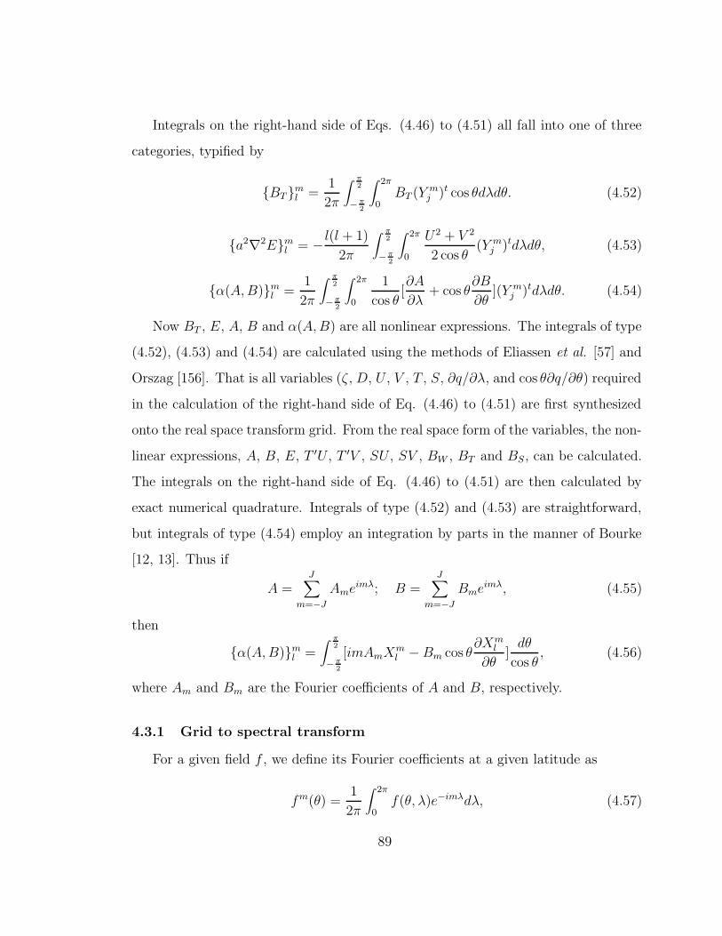
Integrals on the right-hand side of Eqs. (4.46) to (4.51) all fall into one of three
categories, typified by
{BT}ml =
1
2π
∫ π2
−π2
∫ 2π
0BT (Y m
j )t cos θdλdθ. (4.52)
{a2∇2E}ml = − l(l + 1)
2π
∫ π2
−π2
∫ 2π
0
U2 + V 2
2 cos θ(Y m
j )tdλdθ, (4.53)
{α(A,B)}ml =
1
2π
∫ π2
−π2
∫ 2π
0
1
cos θ[∂A
∂λ+ cos θ
∂B
∂θ](Y m
j )tdλdθ. (4.54)
Now BT , E, A, B and α(A,B) are all nonlinear expressions. The integrals of type
(4.52), (4.53) and (4.54) are calculated using the methods of Eliassen et al. [57] and
Orszag [156]. That is all variables (ζ, D, U , V , T , S, ∂q/∂λ, and cos θ∂q/∂θ) required
in the calculation of the right-hand side of Eq. (4.46) to (4.51) are first synthesized
onto the real space transform grid. From the real space form of the variables, the non-
linear expressions, A, B, E, T ′U , T ′V , SU , SV , BW , BT and BS, can be calculated.
The integrals on the right-hand side of Eq. (4.46) to (4.51) are then calculated by
exact numerical quadrature. Integrals of type (4.52) and (4.53) are straightforward,
but integrals of type (4.54) employ an integration by parts in the manner of Bourke
[12, 13]. Thus if
A =J
∑
m=−J
Ameimλ; B =
J∑
m=−J
Bmeimλ, (4.55)
then
{α(A,B)}ml =
∫ π2
−π2
[imAmXml − Bm cos θ
∂Xml
∂θ]dθ
cos θ, (4.56)
where Am and Bm are the Fourier coefficients of A and B, respectively.
4.3.1 Grid to spectral transform
For a given field f , we define its Fourier coefficients at a given latitude as
fm(θ) =1
2π
∫ 2π
0f(θ, λ)e−imλdλ, (4.57)
89
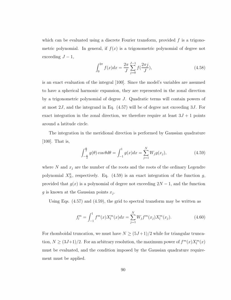
which can be evaluated using a discrete Fourier transform, provided f is a trigono-
metric polynomial. In general, if f(x) is a trigonometric polynomial of degree not
exceeding J − 1,∫ 2π
0f(x)dx =
2π
J
J−1∑
j=0
f(2πj
J), (4.58)
is an exact evaluation of the integral [100]. Since the model’s variables are assumed
to have a spherical harmonic expansion, they are represented in the zonal direction
by a trigonometric polynomial of degree J . Quadratic terms will contain powers of
at most 2J , and the integrand in Eq. (4.57) will be of degree not exceeding 3J . For
exact integration in the zonal direction, we therefore require at least 3J + 1 points
around a latitude circle.
The integration in the meridional direction is performed by Gaussian quadrature
[100]. That is,
∫ π2
−π2
g(θ) cos θdθ =∫ 1
−1g(x)dx =
N∑
j=1
Wjg(xj), (4.59)
where N and xj are the number of the roots and the roots of the ordinary Legendre
polynomial X0N , respectively. Eq. (4.59) is an exact integration of the function g,
provided that g(x) is a polynomial of degree not exceeding 2N − 1, and the function
g is known at the Gaussian points xj.
Using Eqs. (4.57) and (4.59), the grid to spectral transform may be written as
fml =
∫ 1
−1fm(x)Xm
l (x)dx =N
∑
j=1
Wjfm(xj)X
ml (xj). (4.60)
For rhomboidal truncation, we must have N ≥ (5J+1)/2 while for triangular trunca-
tion, N ≥ (3J+1)/2. For an arbitrary resolution, the maximum power of fm(x)Xml (x)
must be evaluated, and the condition imposed by the Gaussian quadrature require-
ment must be applied.
90
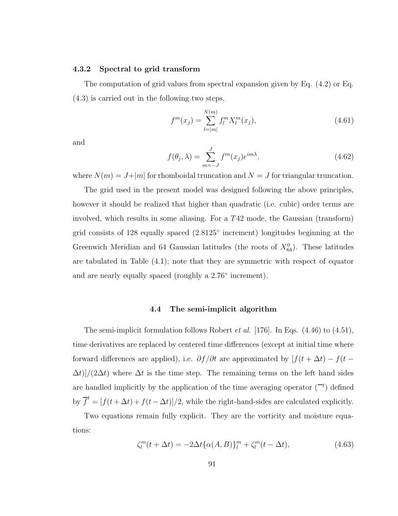
4.3.2 Spectral to grid transform
The computation of grid values from spectral expansion given by Eq. (4.2) or Eq.
(4.3) is carried out in the following two steps,
fm(xj) =N(m)∑
l=|m|
fml X
ml (xj), (4.61)
and
f(θj, λ) =J
∑
m=−J
fm(xj)eimλ, (4.62)
whereN(m) = J+|m| for rhomboidal truncation andN = J for triangular truncation.
The grid used in the present model was designed following the above principles,
however it should be realized that higher than quadratic (i.e. cubic) order terms are
involved, which results in some aliasing. For a T42 mode, the Gaussian (transform)
grid consists of 128 equally spaced (2.8125◦ increment) longitudes beginning at the
Greenwich Meridian and 64 Gaussian latitudes (the roots of X064). These latitudes
are tabulated in Table (4.1); note that they are symmetric with respect of equator
and are nearly equally spaced (roughly a 2.76◦ increment).
4.4 The semi-implicit algorithm
The semi-implicit formulation follows Robert et al. [176]. In Eqs. (4.46) to (4.51),
time derivatives are replaced by centered time differences (except at initial time where
forward differences are applied), i.e. ∂f/∂t are approximated by [f(t + ∆t) − f(t −∆t)]/(2∆t) where ∆t is the time step. The remaining terms on the left hand sides
are handled implicitly by the application of the time averaging operator ( t) defined
by ft= [f(t+∆t)+ f(t−∆t)]/2, while the right-hand-sides are calculated explicitly.
Two equations remain fully explicit. They are the vorticity and moisture equa-
tions:
ζml (t + ∆t) = −2∆t{α(A,B)}m
l + ζml (t− ∆t), (4.63)
91
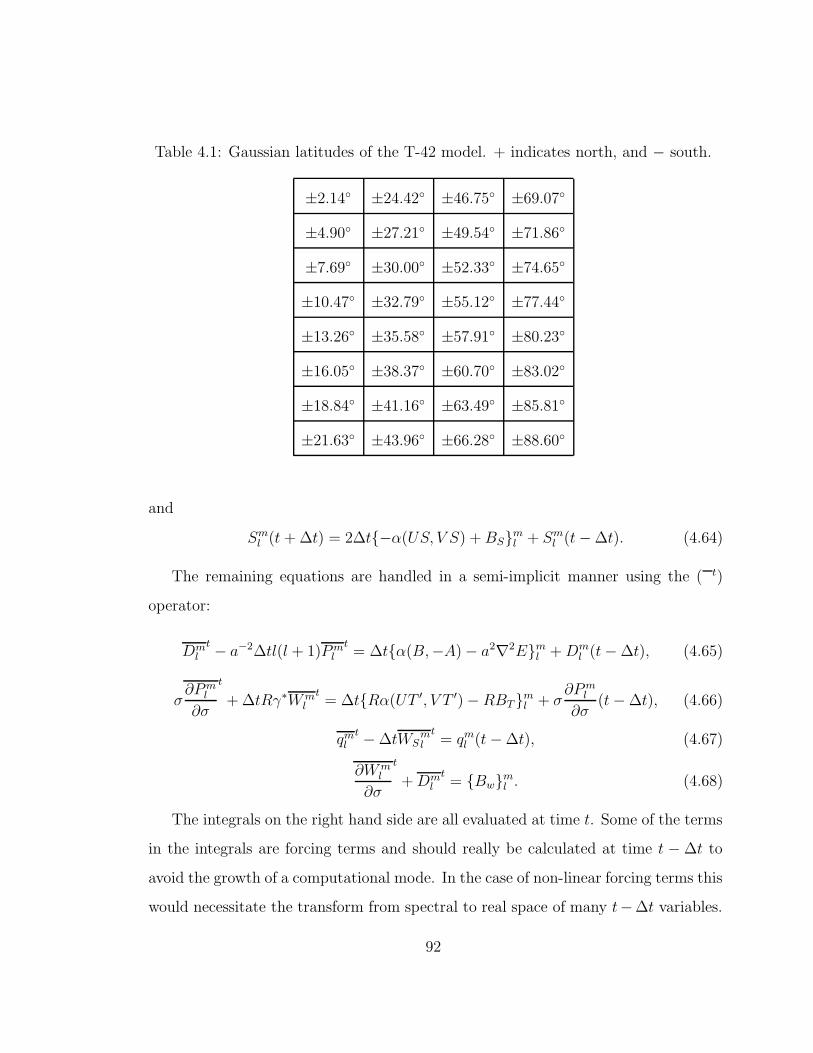
Table 4.1: Gaussian latitudes of the T-42 model. + indicates north, and − south.
±2.14◦ ±24.42◦ ±46.75◦ ±69.07◦
±4.90◦ ±27.21◦ ±49.54◦ ±71.86◦
±7.69◦ ±30.00◦ ±52.33◦ ±74.65◦
±10.47◦ ±32.79◦ ±55.12◦ ±77.44◦
±13.26◦ ±35.58◦ ±57.91◦ ±80.23◦
±16.05◦ ±38.37◦ ±60.70◦ ±83.02◦
±18.84◦ ±41.16◦ ±63.49◦ ±85.81◦
±21.63◦ ±43.96◦ ±66.28◦ ±88.60◦
and
Sml (t + ∆t) = 2∆t{−α(US, V S) +BS}m
l + Sml (t− ∆t). (4.64)
The remaining equations are handled in a semi-implicit manner using the ( t)
operator:
Dml
t − a−2∆tl(l + 1)Pml
t= ∆t{α(B,−A) − a2∇2E}m
l +Dml (t− ∆t), (4.65)
σ∂Pm
l
∂σ
t
+ ∆tRγ∗Wml
t= ∆t{Rα(UT ′, V T ′) − RBT}m
l + σ∂Pm
l
∂σ(t− ∆t), (4.66)
qml
t − ∆tWSml
t= qm
l (t− ∆t), (4.67)
∂Wml
∂σ
t
+Dml
t= {Bw}m
l . (4.68)
The integrals on the right hand side are all evaluated at time t. Some of the terms
in the integrals are forcing terms and should really be calculated at time t − ∆t to
avoid the growth of a computational mode. In the case of non-linear forcing terms this
would necessitate the transform from spectral to real space of many t−∆t variables.
92
This is undesirable from the point of view of computational efficiency, so we have
chosen to calculate certain forcing terms at time t and suppress the computational
mode with a very weak time filter [7].
In the manner of Robert et al. [176], Dml
tis eliminated between Eqs. (4.65) and
(4.68). Then Wml
tis eliminated between the resulting equation and Eq. (4.66) giving
a diagnostic equation for Pml
t
∂
∂σ
σ
γ∗∂Pm
l
∂σ
t
− R∆t2
a2l(l + 1)Pm
l
t=
∂
∂σ
{CT
γ∗
}m
l+ {CD}m
l , (4.69)
where
{CT}ml = R∆t{α(UT ′, V T ′) − BT}m
l + σ∂Pm
l
∂σ(t− ∆t), (4.70)
and
{CD}ml = R∆t{BW − ∆tα(B,−A) + a2∆t∇2E}m
l
+ R∆tDml (t− ∆t). (4.71)
Thus, Eqs. (4.65) to (4.68) have been reduced to a two-point boundary value
problem for each horizontal mode. If {CT}ml and {CD}m
l are known at time t, the
Pml
tcan be calculated for each m, l provided the boundary conditions at σ = 0 and
σ = 1 are given. The remaining variables Dml
t, Wm
l
t, WS
ml
t, qm
l
tcan be calculated by
back substitution into Eqs. (4.65) to (4.68) and the same variables at t+∆t can then
be calculated from the definition of the ( t) operator. Discussion of the appropriate
boundary condition for the solution of Eq. (4.69) will be delayed until the vertical
discretization has been introduced in the next section.
It is appropriate at this time to comment briefly upon the semi-implicit algorithm
just derived, since it might appear that certain non-linear terms are being handled
implicitly. Thus, at first sight, it appears that the non-linear term G is being included
on the left hand (implicit) side of Eq. (4.33) because of the definition for W given in
Eq (4.30). This is not so, as was pointed out by Asselin [7], because the equation for
93
W that is actually used in the model is Eq. (4.35), in which the non-linear term G is
on the right-hand (explicit) side. Thus, the introduction of the variable W does not
allow the implicit treatment of some non-linear terms, but it is convenient, as will be
demonstrated subsequently.
4.5 Vertical discretization
The vertical finite-difference scheme is a somewhat more general form of the
scheme used by Robert et al. [176]. The basic feature of the scheme is that the
temperatures are carried at levels intermediate to the levels of the geopotentials. We
will dwell principally on the finite-difference analogues to the left-hand-sides of Eqs.
(4.65)-(4.69). The vertical finite-differencing involved in the right-hand-sides of these
equations is conventional and will not be discussed in length. It should be stated,
though, that logarithmic vertical differencing has generally been used, in particular
94
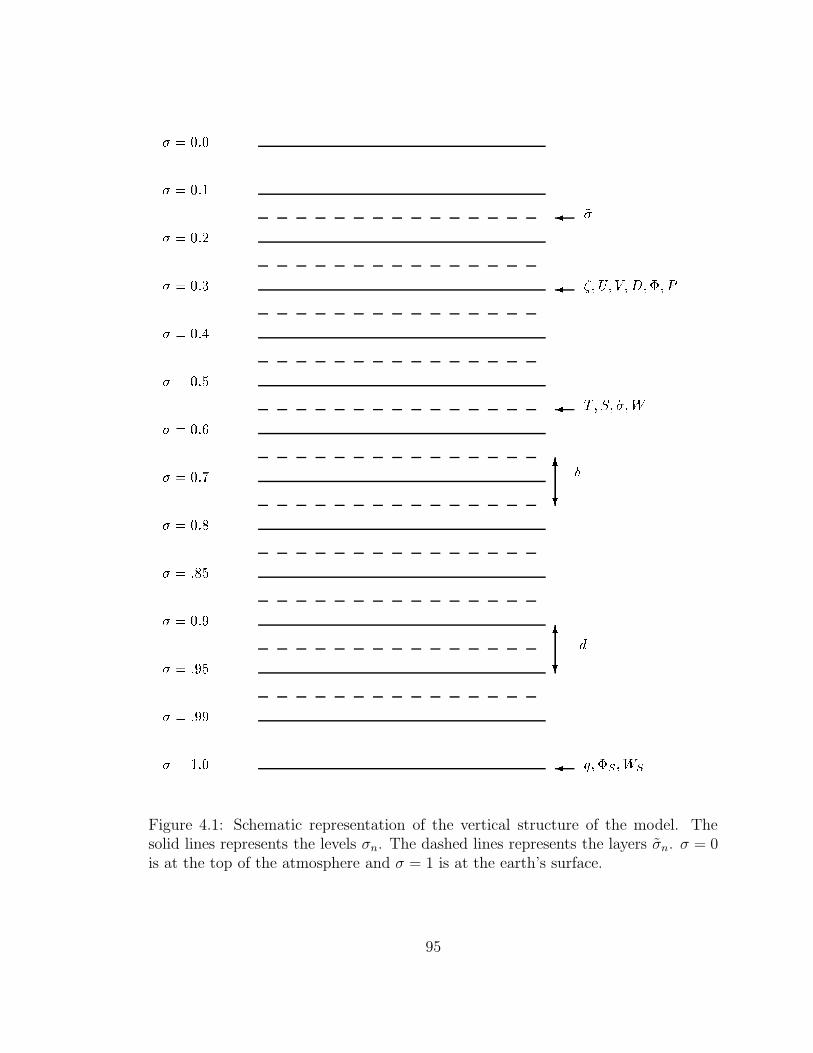
���������
�������� ��
���������
�������� ���������������������
���������
��������� ��"!#��$� ��%
��������&
'( )
�������+*
��������,
���-��,.�
��������/
'( 0
���-��/.�
���-��/./
���-�.��� 12�3�546��%74
Figure 4.1: Schematic representation of the vertical structure of the model. Thesolid lines represents the levels σn. The dashed lines represents the layers σn. σ = 0is at the top of the atmosphere and σ = 1 is at the earth’s surface.
95
with respect to the thermodynamic variables. To simplify the notation, the subscript
l and superscript m will be assumed. Thus, fml is written as f , and {f}m
l as {f}.The levels (in σ) of the FSUGSM are placed as shown in Fig. 4.1. This is a twelve-
level model. Note (in Fig. 4.1) the vertical staggering of the levels, where ζ, D and
P (hence, also U , V and Φ) are defined at levels shown by solid lines (here after
referred to as the σ-levels) while T , S and W (also σ) are defined at levels indicated
by dashed lines (hence after referred to as the σ-levels). Second order accuracy for
the hydrostatics demands that the σ-levels be located midway between the σ-levels
in the ln σ coordinate, thus
ln σk =ln σk + ln σk+1
2, (4.72)
which implies
σk =√σkσk+1, k = 1, . . . , N (4.73)
where the subscripts refer to the level in question and N , the index of the bottom
model level, is equal to 12. Note also in Fig. 4.1 that the increment of the σ-levels is
0.1 above σ = 0.8 and becomes smaller below σ = 0.8, which affords greater vertical
resolution in the planetary boundary layer.
The thermodynamic equation is applied at intermediate levels. These levels are
obtained from a finite difference form of the hydrostatic equation. The following finite-
difference approximation to the hydrostatic equation (4.47) is second-order accurate,
provided that the layer temperatures Tn are defined as the geometric mean of the
adjacent σ-level values, i.e. by
Tn =Φn − Φn+1
Rdn
, n = 1, . . . , N, (4.74)
where
Φn = Φ(σ = σn), dn = ln(σn+1/σn). (4.75)
96
We will hereafter refer to the σ-values, defined by Eq. (4.73) where the thermody-
namic equation is applied, as the layer values. The tilde (∼) will be used to indicate
which variables are carried in the layers (σ = σn); these are Tn, Sn, and Wn. Note
that WN is not carried; instead we use Ws which is applied at a level σN+1 = 1 and
therefore appears without a tilde.
It is convenient to define vertical increments in σ; i.e.
δn = σn+1 − σn, n = 1, . . . , N − 2. (4.76)
Both the top and bottom increments are special cases. Thus
δ0 = σ1 δN−1 = 1 − σN−1. (4.77)
Now Pn = Φn + RT ∗nq is defined on the σn levels, whereas the temperatures Tn
and thus T ∗n are carried in the σn layers. We obtain T ∗
n and thus Pn from T ∗n and q
by simply taking the logarithmic average of the adjacent layer temperatures T ∗n and
T ∗n+1. To second order accuracy
T ∗n =
dn−1T∗n + dnT
∗n−1
dn−1 + dn
, 2 ≤ n ≤ N. (4.78)
T ∗1 can not be calculated in this manner and is instead simply obtained by linear
extrapolation.
T ∗1 = 1.5T ∗
1 − 0.5T ∗2 , (4.79)
The T ′n are obtained in a similar manner.
The static stability γ∗ can be calculated at the σn layers simply as
γ∗n =1
σn
(
RT ∗n
Cp
− T ∗n+1 − T ∗
n
dn
)
, n = 1, . . . , N (4.80)
where T ∗N+1 = T ∗
s . In the absence of an equation for Ts, it has been assumed that
γ∗N = γ∗N−1. This, in effect, formally defines T ∗s in terms of T ∗
N and T ∗N . A similar
expression and assumption is used to relate γ ′n to T ′
n, T ′n and T ′
n+1.
97
Vertically discretized analogues of the vertical integration operators ( σ) and ( )
defined in Eq. (4.6) are required for the calculation of G, D, Gσ, Dσ and ultimately
σ from σ = (σ − 1)(D + V · ∇q) + Dσ + V σ · ∇q and Eq. (4.24) at σn layers. The
vertical integral F σ is approximated by F n, a simple quadrature extending from the
surface (σ = 1) to σn. F is approximated by F 0, the same quadrature extending from
σ = 1 to σ = 0. Thus, if F is a level variable, the approximation for F σ at σ = σn is
F n =N
∑
k=n+1
Fkδk−1, n = 1, . . . , N − 1 (4.81)
and the approximation for F is
F 0 =N
∑
k=1
Fkδk−1. (4.82)
In this manner it is possible to obtain the quadrature analogues of G, D, Gσ,
Dσ and thus σ at each of the layers σn, 1 ≤ n ≤ N − 1. At σN we have assumed
˜σN = h ˜σN−1 where h is an empirical constant 0 ≤ h ≤ 1.
Similar approximations are used for any remaining terms on the right-hand-sides
of Eqs. (4.65-4.69).
All that remains to be discussed is the solution of the boundary value problem
(4.69). The consistent vertically discretized form of this equation for 2 ≤ n ≤ N − 1
is
1
δn−1
[(
Pn+1t − Pn
t
γ∗ndn
)
−(
Pn − Pn−1t
γ∗n−1dn−1
)]
− R∆t2
a2l(l + 1)Pn
t=
1
δn−1
[
1
γ∗n{CT}n − 1
γ∗n−1
{CT}n−1
]
+ {CD}n, (4.83)
where, as mentioned previously, n refers to level or layer, (˜) indicates a layer value,
and { } refers to a horizontal integration (Eq. (4.5)).
Eq. (4.83) yields N − 2 equations in the N unknowns Pnt, 1 ≤ n ≤ N . To close
the system it is necessary to obtain two additional equations involving respectively
P1tand PN
t.
98
The top boundary condition is straightforward to apply. At σ = 0, σ = 0, which
implies W = 0 in the finite difference analogue of Eq. (4.68) applied at σ1. This leads
to the following equation relating W1
t
to D1t:
W1
t
δ0+D1
t= {Bw}1. (4.84)
Combining the above equations with finite difference analogues of equations (4.65)
and (4.66), applied at σ1 and σ1 respectively, yields an equation involving P1tand P2
t
only:
1
δ0
(
P2t − P1
t
γ∗1d1
)
− R∆t2
a2l(l + 1)P1
t=
{CT}δ0γ
∗1
+ {CD}1. (4.85)
To close the system at the bottom boundary is less straightforward. Recalling
the definition of W and assumptions made for γN and ˜σN and noting that ΦS is time
invariant, it can be shown that the finite difference analogue of Eq. (4.66) degenerates
into the following form when applied at σN .
−PNt
λ∗NdN
+R∆t
λ∗Nhγ∗N−1WN−1
t
+R∆tWS
t
={CT}N
λ∗N, (4.86)
where
λ∗N =RT ∗
N
Cp
+T ∗
N
dN
− hγ∗N−1σN−1, (4.87)
The finite difference analogues of Eqs. (4.65) and (4.68) applied at σN yield a relation
between WSt, WN−1
t
and PNt. A third relation between PN−1
t, PN
tand WN−1
t
can
be obtained by applying the finite difference analogue of Eq. (4.66) at ˜σN−1. This
yields 3 equations in 4 unknowns PN−1t, PN
tand WN−1
t
and WStwhich can be used
to obtain a single equation in PN−1tand PN
t; i.e.
1
δN−1
[−PNt
λ∗NdN
−(
PN − PN−1t
λ∗N−1dN−1
)]
− R∆t2
a2l(l + 1)PN
t=
1
δN−1
[
1
λ∗N{CT}N − 1
λ∗N−1
{CT}N−1
]
+ {CD}N , (4.88)
99
where
λ∗N−1 =γ∗N−1λ
∗N
λ∗N + hγ∗N−1
. (4.89)
Eqs. (4.83), (4.85) and (4.88) define a N ×N tridiagonal matrix relationship for
each horizontal mode (m, l) of the Pnt, 1 ≤ n ≤ N . These matrix problems are easily
solved by an efficient tridiagonal matrix algorithm of the Thomas algorithm variety.
Once the Pnt
have been calculated, back substitution into the vertically discretized
forms of Eqs. (4.65) and (4.66) yields Dntand Wn
t
, respectively. Substitution of Pnt
and Wn
t
into Eq. (4.86) yields WSt, from which qt can be obtained using Eq. (4.67).
The definition of the ( t) operator then yields Pn(t+ ∆t), Dn(t+ ∆t) and q(t+ ∆t).
The remaining variables Φn(t+∆t) and Tn(t+∆t) are calculated diagnostically using
vertically discretized forms of Eqs. (4.44) and (4.45). The explicit prognostic Eqs.
(4.63) and (4.64) yield ζn(t+ ∆t) and Sn(t+ ∆t).
This formulation of the semi-implicit method does have the advantage of yielding
a tridiagonal matrix in the vertical at the expense of some conceptual complication.
However, the extra calculations per time step due to the semi-implicit calculation are
completely negligible.
The physical processes included in the FSUGSM are described in Appendix F.
100
CHAPTER 5
4-D VARIATIONAL DATA ASSIMILATION WITH THE FSU
GLOBAL SPECTRAL MODEL
5.1 Introduction
The numerical feasibility of variational data assimilation has been extensively
demonstrated for 2-D models, but has only recently been applied to 3-D models
[11, 38, 54, 157, 168, 169, 170, 171, 233]. The objective of the current chapter is to
demonstrate the feasibility of 4-D variational data assimilation applied to an adiabatic
version of the FSUGSM. The number of components of the control variables vector
(the initial conditions vector) is 303104. As stated before the numerical cost of the 4-
D VDA originates both from the model integration and the gradient calculation of the
cost function with respect to the control variables. With present numerical models,
numerical algorithms and presently available computer power, the only practical way
to carry out the 4-D VDA is through an appropriate use of the adjoint techniques in
calculating the gradient of the cost function with respect to the control variables [35].
The adjoint techniques were developed in the fields of optimal control theory of PDEs
of distributed parameters [116], and their application to 4-D VDA requires to obtain
the gradient of the cost function with respect to the control variables which is obtained
by one backwards integration of the adjoint model in time. Therefore, we first develop
the TLM and the adjoint model of a dry version (i.e., no physical effects are involved
except horizontal diffusion) of the FSUGSM and verify their accuracies in Section 5.2.
The dry version of the FSUGSM is used because we do not want to add, at this stage,
101
the complexity inherent in the inclusion of effects of highly nonlinear and threshold on-
off diabatic physical parameterizations, which are still at the research stage [216, 231,
236]. The numerical algorithms employed in 4-D VDA and related scaling issues are
discussed in Section 5.3. In Section 5.4, various variational assimilation experiments
are conducted. The ability of 4-D VDA to retrieve observational fields is investigated
starting from either shifted or randomly perturbed initial conditions. We evaluate the
impacts of different observations distributed in space and time as well as the impact
of the horizontal diffusions. Through different scenarios of sets of observations, we
demonstrate the efficiency of 4-D VDA in extracting the information contained in the
dynamics of the model together with information in the observations. Conclusions
as well as topics for further research related to the 4-D VDA with FSUGSM are
presented in Section 5.5.
5.2 Model developments and numerical validation
5.2.1 The cost function and its gradient with respect to control variables
The cost function will be defined in physical space rather than in spectral space
because it is clearer and easier to implement proper scaling in physical space than
in spectral space. Therefore the cost function is still defined by Eq. 1.3 where W is
an N ×N diagonal weighting matrix with W~ζ, W ~D, W~S, W~q, and W~T as its diagonal
sub-matrices entries of weighting factors for vorticity, divergence, moisture, surface
pressure, and temperature fields, respectively. Here N = L(4K + 1) is the number
of components of the state vector ~X, K is the number of vertical levels and L is the
number of Gaussian grid points. ~X = (~ζ, ~D, ~S, ~q, ~T )t denotes the state vector, where
~ζ, ~D, ~S, ~q, ~T contain values of vorticity, divergence, moisture, surface pressure, and
temperature over all grid points on all levels at time t. ~Xo = (~ζo, ~Do, ~So, ~qo, ~T o)t,
denotes the observation vector where ~ζo, ~Do, ~So, ~qo, ~T o are observational values of
102
vorticity, divergence, moisture, surface pressure, and temperature over all grid points
on all levels at time t. F is a vector function with five components being the right
hand sides of vorticity, divergence, thermodynamic, surface pressure tendency and
moisture equations (4.7 – 4.7 and 4.12).
The 4-D variational data assimilation problem (1.1) is usually solved by using
large-scale unconstrained minimization algorithms such as LBFGS of Liu and Nocedal
[117], truncated-Newton [130], the adjoint truncated-Newton [219] and quasi-Newton
algorithms. All these minimization algorithms require the calculation of the gradient
of the cost function with respect to control variables. The current studies will ob-
tain the gradient of the cost function by using the adjoint model techniques. Other
alternatives for obtaining the gradient of the cost function such as automatic differ-
entiation ([55], [69]), analytical evaluation and finite-difference (FD) approximations
exist. However, they are either not feasible for this optimal control problem applied
to VDA or are too costly to apply.
The adjoint model of Eqs. (1.10) and (1.10) is defined as
−∂X∂t
= (∂F
∂ ~X)∗X, (5.1)
X(tf) = U ′′, (5.2)
where X is the adjoint variable and (·)∗ denotes the complex conjugate transpose.
The FOA model of Eqs. (1.10) and (1.11) is defined by Eqs. (2.2) and (2.3).
Clearly the FOA model given by Eq. (2.2) can be obtained by adding a forcing term
to the adjoint model given by Eq. (5.1) and setting the final condition (5.2) to zero.
One can prove that the gradient of the cost function with respect to the initial
conditions is equal to the value of the FOA model variable at the initial time
∇UJ = P (t0), (5.3)
(see Section 1.3 and [149, 202, 218]).
103
5.2.2 The accuracy of the tangent linear model
The TLM model of the adiabatic FSUGSM was developed and its validity was
verified. The TLM model is the result of the linearization of the direct adiabatic
FSUGSM in the vicinity of a given model trajectory [113]. If we view the direct
adiabatic FSUGSM as, M , the result of multiplication of a number of matrices:
M = A1A2...AN , (5.4)
where each matrix Ai (i = 1, ..., N) represents either a subroutine or a single do loop,
then the TLM model can be viewed as T lm
T lm = B1B2...BN , (5.5)
where Bi = Ai if Ai is linear and Bi is a linearization of Ai in the vicinity of a basic
state of ~X if Ai is nonlinear for i = 1, ..., N .
Suppose that U ′1 and U ′
2 are two initial conditions for the TLM model then
B1B2...BN (U ′1 + U ′
2) = B1B2...BN (U ′1) +B1B2...BN(U ′
2). (5.6)
Eq. (5.6) can be used as a preliminary criterion for the correctness-check of the TLM
model.
For a given state variable U , and a perturbation, U ′ on U , the real evolution of
the solution due to a perturbation αU ′ is given by
M(U + αU ′) −M(U) (5.7)
where α is a scalar and M(U) represents the numerical integration of the direct
adiabatic FSUGSM starting from the initial conditions U . If T lm(αU ′) represents
the numerical integration of the TLM models starting from the initial conditions αU ′,
then according to the definition of the TLM one obtains
ψ(α) =‖M(U + αU ′) −M(U)‖
‖T lm(αU ′)‖ = 1.+O(α‖U ′‖), (5.8)
104
where ‖ · ‖ denotes the Euclidean norm of “·”.
We take the fields of vorticity, divergence, moisture, surface pressure, and tem-
perature at 0 UTC 1 June 1988 as U , and choose U ′ = αU where α is small scalar
but not too close to the machine accuracy. The direct adiabatic FSUGSM and TLM
models are integrated for an hour with various α values. Fig 5.1 indicates that the
TLM model produced a good asymptotic approximation to the evolution of perturba-
tions for the forecast period when α varies from 10−7 to 1. It is surprising that even
for perturbations with magnitudes similar to that of U , the TLM model still yields
a relatively good approximation to the evolution of perturbations for the forecast
period.
When the forecast period is increased to 6 hours, the results shown in Fig 5.1 are
still correct. For instance, when α = 0.1, ψ(α) = 0.9995405246. Therefore the TLM
is correct for reasonable long forecast period and for perturbations with magnitudes
similar to that of the initial condition of the nonlinear model. So the correctness of
the TLM model has been verified.
5.2.3 The accuracy of the first order adjoint model
The adjoint model of Eq. (5.5) can be obtained by taking its complex conjugate
i.e.
T lmt = Bt1B
t2...B
tN . (5.9)
In this way, the discrete adjoint model can be directly derived from the discrete linear
model, which in turn is derived from the FSUGSM by linearization around a basic
state. This simplifies not only the complexity of constructing the adjoint model but
also avoids the inconsistency generally arising from the derivation from the adjoint
equations in analytic form followed by the discrete approximation.
105
The correctness of the adjoint model can be checked in three ways. First, at any
level of the code, the adjoint code can be checked by using the following identity
(BQ)t(BQ) = Qt[Bt(BQ)], (5.10)
where B and Q represent any code and its input in the discrete TLM model, respec-
tively. For example, if B = T lm, the initial condition Q of the TLM model is chosen
as the basic state ~X at 0 UTC 1 June 1988, the basic states at later times are ob-
tained by integrating the FSUGSM starting with the same initial condition Q and all
models are integrated for six hours, then Bt(BQ) denotes the backwards integration
of the adjoint model given by Eq. (5.1) with final condition taken as the output of
the TLM model integration, then one obtains
(BQ)t(BQ) = 1.0189576063747× 10¹³, (5.11)
Qt[Bt(BQ)] = 1.0189576063753× 10¹³, (5.12)
which prove the correctness of the discrete adjoint model given by Eq. (5.9) up to
the machine’s precision of 14 digits.
Second, the TLM describes the evolutions of perturbations in a forecast model.
Eq. (5.10) indicates that the accuracy of the TLM is the same as that of its adjoint
model given by Eq. (5.9) or (5.1)-(5.1). This can also be demonstrated intuitively by
the following experiment.
Let observations consist of a full-model-state vector at the end of the assimilation
period, then the cost function assumes the following form
J(U) =< W ( ~X(tf ) − ~Xo(tf)), ( ~X(tf) − ~Xo(tf)) > . (5.13)
If we denote ∆J(U) as a first order approximation to J(U + U ′) − J(U) due to the
change U ′ in the initial condition U , and T lm as the numerical integrations of the
106
TLM, then
J(U + U ′) − J(U) ≈ ∆J(U) =∂J( ~X(tf))
∂ ~X(tf )· ∆ ~X(tf )
≈ ∂J( ~X(tf ))
∂ ~X(tf)· T lm(U ′)
= U ′t · T lmt(∂J( ~X(tf))
∂ ~X(tf )) = U ′t · ∇UJ, (5.14)
where the superscript t denotes a transpose and ∆ ~X(tf) is the change in the state
variable ~X at the final time tf due to the change U ′ in the initial condition U , i.e.
given U and U ′ then identical values of ∆J(U) are obtained whether the TLM or its
adjoint model is applied, implying both values are equally accurate [58].
Still, it is worthwhile to provide an example of the accuracy of an adjoint calcula-
tion, especially since we will claim that the accuracy is much better than one would
have expected.
Suppose that the cost function is defined as the difference between the model
solution and the observation at the final time (six hours from the initial time) and
the observation is taken as a full-state vector solution at a time which is twelve hours
apart from the initial time. The weighting factor for divergence field is calculated
according to the following formula
W ~D =1
4‖ ~D(tf ) − ~Do(tf )‖2, (5.15)
with similar expressions for the moisture, temperature, surface pressure, and vorticity
fields. The term ∂J( ~X(tf ))/∂ ~X(tf ) in Eq. (5.14) is obtained by integrating the
forward model and using the above specified weighting factors, i.e.
∂J( ~X(tf))
∂ ~X(tf )= 2W ( ~X(tf ) − ~Xo(tf)), (5.16)
The initial condition for the TLM model is taken as ∂J( ~X(tf))/∂ ~X(tf), i.e.
U ′ =∂J( ~X(tf))
∂ ~X(tf )(5.17)
107
∂J( ~X(tf))/∂ ~X(tf) is also used as the final condition for the adjoint model given by
Eqs. (5.1)-(5.1). If the perturbation is applied to an six hour forecast, then
∂J( ~X(tf ))
∂ ~X(tf )· T lmU ′
U ′t · T lmt(∂J( ~X(tf ))
∂ ~X(tf ))
=0.00040447305742735
0.00040447305742624= 1.000000000003, (5.18)
which proves numerically that both the TLM and its adjoint model are correct and
have the same accuracy.
Third, the verification of the correctness of the gradient can be conducted as
described below. The Taylor formula applied in the direction U ′ = ∂J(U)/∂ ~X(tf)
yields
φ(α) =J(U + αU ′) − J(U)
αU ′t · ∇UJ= 1.+O(α‖U ′‖). (5.19)
For small α but not too close to the machine accuracy, the value of φ(α) should be
close to one if the gradient ∇UJ is correctly calculated. Fig 5.2 shows that for α in
the range between 10−3 and 10−14 an unit value of φ(α) is obtained.
5.3 Descent algorithms and scaling
5.3.1 The LBFGS algorithm of Liu and Nocedal
Liu and Nocedal [117] compared the combined conjugate-gradient quasi-Newton
method of Buckley and LeNir [14], the limited-memory quasi-Newton method de-
scribed by Nocedal [154] (called LBFGS method), and the partitioned quasi-Newton
method of Griewank and Toint [76]. Zou et al. [227] compared four of the state-
of-the-art limited-memory quasi-Newton methods on several test problems, including
problems in meteorology and oceanography. Their results show that the LBFGS al-
gorithm is the most efficient and particularly robust amongst the algorithms tested
for the set of problems considered here. Therefore the LBFGS algorithm is chosen
for this study since it deals with the critical issue of storage in large-scale problems.
108
In the LBFGS algorithm, the user provides a sparse symmetric and positive definite
matrix H0, which approximates the inverse Hessian of the cost function, and spec-
ifies the number m of the quasi-Newton up-dates, therefore controls the amount of
the storage required. The LBFGS algorithm updates the formula generated matrices
which approximate the Hessian by building curvature information using information
from the last m quasi-Newton iterations. After having used the m vector storage lo-
cations for m quasi-Newton updates of the Hessian, the quasi-Newton approximation
of the Hessian matrix is updated by dropping the oldest update vector and replacing
it with the newest update vector. A new line search direction, which is an estimate of
the relative change to the current variables vector that produces the maximum reduc-
tion in the cost function, is then computed. It employs a cubic line search required
to satisfy a Wolfe condition [224], and an unit step size is always tried first. For a
precise description of the LBFGS algorithm, please see [117].
5.3.2 Weighting and scaling
Weights in the cost function have a serious impact on the minimization algorithm
[26]. A poor set of weights may result in elongated contour lines of the cost function,
or even in a total failure of the VDA. There are several ways to determine weights
such as: (1) trial and error method [110], (2) the statistical method, i.e. taking the
reciprocal of the variance of the observation errors [32], and (3) temporal weighting
method [34]. The first method may be very costly since it depends on both luck
and experience. In the second method, the variances are difficult to specify properly,
and much more research work is necessary in this area. In the third method weights
are assigned to individual observations and vary linearly with time. The total sum
of the weights assumes the same value as the reciprocal of squared estimates of the
statistical root-mean-square observational error.
109
In our experiments with FSUGSM, a diagonal weighting matrix
W = diag{W~ζ,W ~D,W~S,W~q,W~T}, (5.20)
is used where W~ζ, W ~D, W~S, W~q, and W~T are constant diagonal sub-matrices. The
diagonal elements of W ~D are calculated according to the following formula
(W ~D)jj =1
4∑M
i=0 ‖ ~D(ti) − ~Do(ti)‖2, (5.21)
with similar expressions for the moisture, temperature, surface pressure, and vorticity
fields. Model solutions are obtained by integrating the model from an initial condition.
Weights given by Eq. (5.21) nondimensionalize the cost function, and result in an
unit cost function at the beginning of the variational data assimilation.
Scaling is a crucial issue in the success of nonlinear unconstrained optimization
problems, and considerable research has been carried out on scaling nonlinear prob-
lems. It is well known that a badly scaled nonlinear programming problem can be
almost impossible to solve [149, 34]. An effective automatic scaling procedure would
ease these difficulties and could also render problems that are well scaled easier to
solve by improving the condition number of their Hessian matrix [205]. Thus scaling
is a crude way of carrying out preconditioning. For more discussion about precondi-
tioning, please see Appendix C and references [134, 236]
In the FSUGSM, the variables in the control vector have enormously different
magnitudes varying over a range of eight orders of magnitude. Typical values of
vorticity, divergence, natural log of the surface pressure and temperature have the
magnitudes of 10−5, 10−6, 10−2 and 100, respectively. Scaling by variable transfor-
mation converts variables from units that reflect the physical properties to units that
display desirable properties for minimization process. Given a diagonal scaling ma-
trix S = diag{S~ζ, S ~D
, S~S, S~q, S~T
} where S~ζ, S ~D
, S~S, S~q, and S~T
are constant diagonal
sub-matrices, the general scaling procedure may be written as
~X = S ~Xs, (5.22)
110
~gs = S~g, (5.23)
Hs = SHS, (5.24)
where H is the Hessian matrix. The constant diagonal elements of sub-matrix S ~D
will be calculated by
maxi,j
|Dj(ti) −Doj (ti)|, (5.25)
and similarly for S~ζ , S~S, S~q, and S~T where Dj(ti) and Doj (ti) are the j-th components
of vectors ~D and ~Do at time ti, respectively.
For complicated functions, difficulties may be encountered in choosing suitable
scaling factors. There is no general rule to determine the best scaling factors for
all minimization problems, and good scaling is problem dependent. A basic rule
is that the variables of the scaled problem should be of similar magnitude and of
order of unity because with in optimization routines convergence tolerances and other
criteria are necessarily based on an implicit definition of “small” and “large”, and,
thus variables with widely varying orders of magnitude may cause difficulties for
some minimization algorithms [73]. One simple direct way to determine the scaling
factor is to use the typical values for different fields. For some problems, the relative
magnitudes of the gradient field components of the cost function differ from each
other by several orders of magnitude. In such cases, it is better to scale the gradient
of the cost function [73, 115].
5.4 Numerical results of the variational data assimilation
Although the accuracies of the TLM and the adjoint model as well as the gradient
calculation of the cost function with respect to the control variables have been veri-
fied, it is of primary importance to ensure that the system as a whole was properly
constructed and that the minimization of the cost function can be performed using
111
a reasonably high-resolution system. Hence, two sets of experiments were designed
using the LBFGS large-scale unconstrained minimization algorithm of Liu and No-
cedal [117]. Both shifted and randomly perturbed initial conditions are used in the
first set of experiments to investigate the efficiency of the 4-D VDA as well as the
impacts of the length of the assimilation on the convergence rate. In the second set of
experiments, the impacts of distributed observations and that of horizontal diffusion
are investigated.
In all experiments a horizontal truncation of T42 with 12 levels in the vertical
direction is used. For the exact variable transformation from spectral space to physical
grid space, or vice versa, a (128 × 64) Gaussian grid was used, and the dimension of
the vector of control variables is 303104. The length of the time assimilation window
is 6 hours unless indicated otherwise. All the routines are coded in single precision
FORTRAN. The runs were made on the CRAY-YMP supercomputer at Florida State
University, for which the relative machine precision ε is approximately 10−14.
5.4.1 Numerical results with shifted initial conditions
The experiments are devised as follows: the model-generated values starting from
an analysis of the real observational data at 6 UTC 1 June 1988 are used as observa-
tions and the initial guess is taken as an analysis of the real observational data at 0
UTC 1 June 1988. We know exactly what the solution is, and the value of the cost
function at the minimum must be zero.
Here we assume the observations are available at every time step of the assimilation
window and the cost function is defined by Eq. (1.3).
In the first experiment the length of the assimilation window is chosen as one
hour. The purpose of this experiment is to verify that all components of the VDA
work properly before we conduct any VDA for a longer window of assimilation.
112
Fig. 5.3 (solid line) displays the variations of the log of the scaled cost func-
tion (Jk/J0) and scaled gradient norm (‖~gk‖/‖~g0‖) with the number of iterations in
the minimization process. It would appear initially that the VDA works numeri-
cally. Indeed, after 65 iterations, the normalized cost function is reduced by 8 orders
of magnitude while the normalized norm of the gradient is reduced by 4 orders of
magnitude.
It is a good idea to consider the difference fields between the retrieved and ref-
erence (observational) fields before and after the minimization process, since these
difference fields measure the ability of the VDA to retrieve the observational fields.
Fig 5.11 shows the difference fields between the retrieved fields of divergence, vorticity,
temperature and natural log of the surface pressure and the reference (observational)
fields at the beginning of the assimilation window after the minimization process.
Comparing with the same difference fields (Fig. 5.6) before the minimization pro-
cess, it is observed that after the minimization the maximum difference values are
reduced by four orders of magnitude in all difference fields of divergence, vorticity,
temperature and natural log of the surface pressure.
If the length of the assimilation is increased to 6 hours, the VDA also works
successfully. The results in Fig 5.3 (dash line) indicate that after 65 iterations, the
normalized cost function is reduced by 2.3 orders of magnitude while the normalized
norm of the gradient is reduced by 1.5 orders of magnitude.
In Fig 5.4, dotted and long dash lines denote the variation of the log of the rms
error between the initial (guess) and exact temperatures with model levels at the
beginning and end of time assimilation window before assimilation. The solid and
dash lines denote the variation of the log of the rms error between the retrieved and
exact temperatures with model levels at the beginning and end of time assimilation
window after carrying out VDA. It is interesting to notice that the above rms error
is reduced by one order of magnitude at the beginning of time assimilation window
113
while by 1.5 orders magnitude at the end of time assimilation window. The different
reduction in rms errors indicates that our metric for the cost function is not optimal.
The consequence is that the shape of the cost function can become strongly elliptic
with respect to the metric used and the gradient of the cost function can even become
almost orthogonal to the direction of the minimum.
The above experiments imply that the longer the assimilation period, the slower
the convergence rate. The slower convergence rate of the minimization in the case
of longer assimilation window results from the worsening of the conditioning of the
Hessian matrix due to the longer model integration. Thus the use of a longer as-
similation window will require more computation not only due to a longer model
integration interval but also due to a slower convergence rate. There should exist an
optimal assimilation length such that the minimization can retrieve the best initial
condition from the observations and the dynamics in the model equations. An inves-
tigation in this direction will be very useful for operational implementation of 4-D
VDA in NWP, along with selective time weighting of the observations.
5.4.2 Numerical results with randomly perturbed initial conditions
The experiments are devised as follows: the model-generated values starting from
an initial condition taken as an analysis of the real observational data at 0 UTC 1 June
1988 are used as observations and the initial guess is obtained by adding a random
perturbation of the above initial condition to itself. The random perturbations are
obtained by using a standard library randomizer RANF on CRAY-YMP and the
magnitudes of the perturbations are at most 10% of the original. Again, we know
exactly what the solution is, and the value of the cost function at the minimum
must be zero. All the random perturbations used in this chapter are of an uniform
distribution.
114
As in the previous subsection we first consider a case where the length of the
assimilation is only one hour and the observations are available at every time step. Fig.
5.8 shows that the VDA performs successfully. After 65 iterations, the normalized
cost function is reduced by more than 8 orders of magnitude while the normalized
norm of the gradient is reduced by 3.8 orders of magnitude.
From Figs. 5.9 and 5.10 it is observed that after the minimization the maximum
difference values are reduced by four orders of magnitude in all difference fields of
divergence, vorticity, temperature and natural log of the surface pressure. It is also
observed that the reductions in the maximum difference values are different at the
beginning and end of the assimilation window. That is the 4-D VDA is more capable
to retrieve information in the observations and in the dynamics of the model at the
end of the assimilation window for our test problem. It is clear that the 4-D VDA
works equally well with either shifted or randomly perturbed initial conditions.
5.4.3 Impact of horizontal diffusion
We have mentioned that the FSUGSM is used in its adiabatic version without
any physical parameterizations package. Only horizontal diffusion of vorticity, diver-
gence and temperature terms is retained. The horizontal diffusion terms impact the
minimization process [114, 207]. We describe now the impact of these terms on the
VDA.
A Laplacian-type of horizontal diffusion is included in the prognostic equations for
the vorticity, divergence and temperature fields, respectively. Thus the diffusion is of
the form K∇2Q, where K is the diffusion coefficient and Q is vorticity or divergence
or temperature. This diffusion is included primarily for numerical reasons, to suppress
the growth of the amplitudes of higher wavenumber components during the forecast.
This phenomenon, called spectral blocking, has been discussed by Machenhauer [125].
It is caused by neglecting the interactions between waves within the truncation limit
115
with those waves which lie outside the truncation limit. The diffusion is applied in
spectral space, in an implicit manner (i.e. to the prognostic variables at time level t+
∆t) to avoid the growth of a computational mode (linear instability). The numerical
values of the diffusion coefficients for vorticity, divergence and temperature fields are
6.0 × 10¹⁵ and 6.0 × 10¹⁶ for weak and strong horizontal diffusions, respectively.
The same experiments as described in Section 5.4.4 where observations are avail-
able at every time step were performed again with strong horizontal diffusion terms
and without horizontal diffusion terms. The experimental results obtained without
the horizontal diffusion terms and with the strong horizontal diffusion terms present
are very similar to these experimental results obtained with weak horizontal diffusion
terms. The variations (Fig. 5.3) of the log of the scaled cost function (Jk/J0) and
scaled gradient norm (‖~gk‖/‖~g0‖) with the number of iterations in the minimization
process are almost identical to these (also see Fig. 5.3) obtained when weak hori-
zontal diffusion terms are applied to the model. Table 5.1 indicates that rms errors
of temperature at different model levels when no diffusion, weak or strong horizontal
diffusion terms are applied in the model, respectively. It is observed that the rms
errors obtained when weak horizontal diffusion terms are applied in the model are
uniformly smaller than these obtained with no diffusion or strong horizontal diffusion
terms present in the model. When strong horizontal diffusion terms are applied in
the model, the rms errors are the largest amongst the rms errors obtained in the three
cases. The maximum and minimum errors occur at the top and the bottom levels,
respectively.
All these results indicate that when weak horizontal diffusion terms are included
in the adiabatic version of the FSUGSM the minimization yields a more accurate
solution of the VDA problem, but when the horizontal diffusion terms become large,
the minimization may yield a less accurate solution of the VDA problem (see Fig.5.3).
116
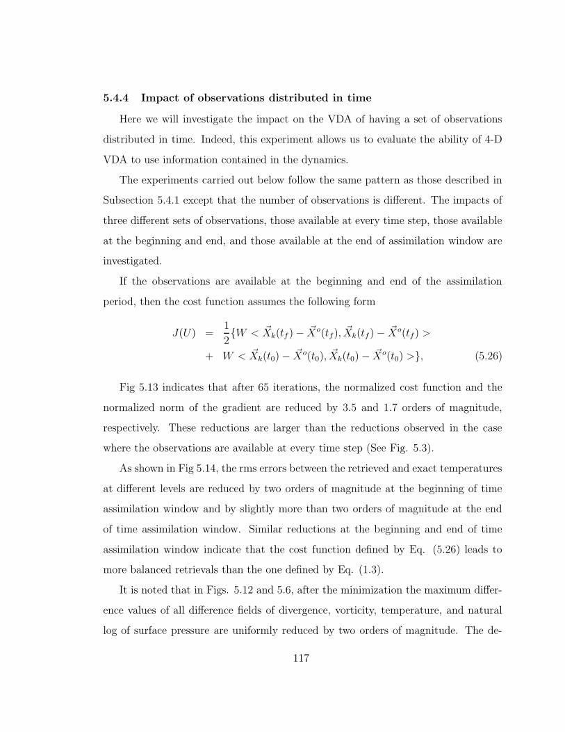
5.4.4 Impact of observations distributed in time
Here we will investigate the impact on the VDA of having a set of observations
distributed in time. Indeed, this experiment allows us to evaluate the ability of 4-D
VDA to use information contained in the dynamics.
The experiments carried out below follow the same pattern as those described in
Subsection 5.4.1 except that the number of observations is different. The impacts of
three different sets of observations, those available at every time step, those available
at the beginning and end, and those available at the end of assimilation window are
investigated.
If the observations are available at the beginning and end of the assimilation
period, then the cost function assumes the following form
J(U) =1
2{W < ~Xk(tf ) − ~Xo(tf), ~Xk(tf ) − ~Xo(tf) >
+ W < ~Xk(t0) − ~Xo(t0), ~Xk(t0) − ~Xo(t0) >}, (5.26)
Fig 5.13 indicates that after 65 iterations, the normalized cost function and the
normalized norm of the gradient are reduced by 3.5 and 1.7 orders of magnitude,
respectively. These reductions are larger than the reductions observed in the case
where the observations are available at every time step (See Fig. 5.3).
As shown in Fig 5.14, the rms errors between the retrieved and exact temperatures
at different levels are reduced by two orders of magnitude at the beginning of time
assimilation window and by slightly more than two orders of magnitude at the end
of time assimilation window. Similar reductions at the beginning and end of time
assimilation window indicate that the cost function defined by Eq. (5.26) leads to
more balanced retrievals than the one defined by Eq. (1.3).
It is noted that in Figs. 5.12 and 5.6, after the minimization the maximum differ-
ence values of all difference fields of divergence, vorticity, temperature, and natural
log of surface pressure are uniformly reduced by two orders of magnitude. The de-
117
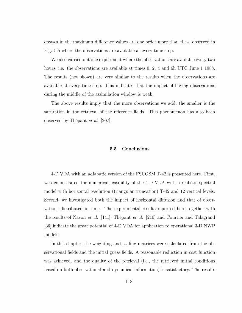
creases in the maximum difference values are one order more than these observed in
Fig. 5.5 where the observations are available at every time step.
We also carried out one experiment where the observations are available every two
hours, i.e. the observations are available at times 0, 2, 4 and 6h UTC June 1 1988.
The results (not shown) are very similar to the results when the observations are
available at every time step. This indicates that the impact of having observations
during the middle of the assimilation window is weak.
The above results imply that the more observations we add, the smaller is the
saturation in the retrieval of the reference fields. This phenomenon has also been
observed by Thepaut et al. [207].
5.5 Conclusions
4-D VDA with an adiabatic version of the FSUGSM T-42 is presented here. First,
we demonstrated the numerical feasibility of the 4-D VDA with a realistic spectral
model with horizontal resolution (triangular truncation) T-42 and 12 vertical levels.
Second, we investigated both the impact of horizontal diffusion and that of obser-
vations distributed in time. The experimental results reported here together with
the results of Navon et al. [141], Thepaut et al. [210] and Courtier and Talagrand
[36] indicate the great potential of 4-D VDA for application to operational 3-D NWP
models.
In this chapter, the weighting and scaling matrices were calculated from the ob-
servational fields and the initial guess fields. A reasonable reduction in cost function
was achieved, and the quality of the retrieval (i.e., the retrieved initial conditions
based on both observational and dynamical information) is satisfactory. The results
118
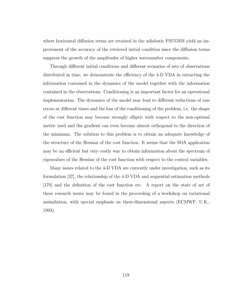
where horizontal diffusion terms are retained in the adiabatic FSUGSM yield an im-
provement of the accuracy of the retrieved initial condition since the diffusion terms
suppress the growth of the amplitudes of higher wavenumber components.
Through different initial conditions and different scenarios of sets of observations
distributed in time, we demonstrate the efficiency of the 4-D VDA in extracting the
information contained in the dynamics of the model together with the information
contained in the observations. Conditioning is an important factor for an operational
implementation. The dynamics of the model may lead to different reductions of rms
errors at different times and the loss of the conditioning of the problem, i.e. the shape
of the cost function may become strongly elliptic with respect to the non-optimal
metric used and the gradient can even become almost orthogonal to the direction of
the minimum. The solution to this problem is to obtain an adequate knowledge of
the structure of the Hessian of the cost function. It seems that the SOA application
may be an efficient but very costly way to obtain information about the spectrum of
eigenvalues of the Hessian of the cost function with respect to the control variables.
Many issues related to the 4-D VDA are currently under investigation, such as its
formulation [37], the relationship of the 4-D VDA and sequential estimation methods
[170] and the definition of the cost function etc. A report on the state of art of
these research issues may be found in the proceeding of a workshop on variational
assimilation, with special emphasis on three-dimensional aspects (ECMWF, U.K.,
1993).
119
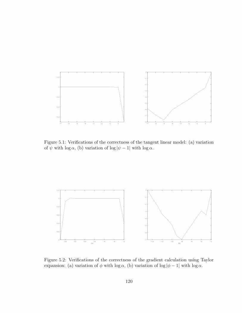
0.4
0.6
0.8
1
1.2
-7 -6 -5 -4 -3 -2 -1 0-8
-7
-6
-5
-4
-3
-2
-1
0
-7 -6 -5 -4 -3 -2 -1 0
Figure 5.1: Verifications of the correctness of the tangent linear model: (a) variationof ψ with logα, (b) variation of log |ψ − 1| with logα.
0
0.2
0.4
0.6
0.8
1
1.2
-14 -12 -10 -8 -6 -4 -2(a)
-7
-6
-5
-4
-3
-2
-1
0
-14 -12 -10 -8 -6 -4 -2(b)
Figure 5.2: Verifications of the correctness of the gradient calculation using Taylorexpansion: (a) variation of φ with logα, (b) variation of log |φ− 1| with logα.
120
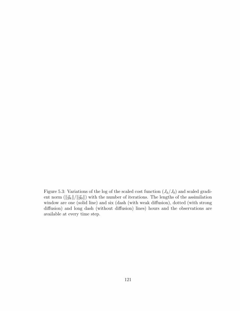
Figure 5.3: Variations of the log of the scaled cost function (Jk/J0) and scaled gradi-ent norm (‖~gk‖/‖~g0‖) with the number of iterations. The lengths of the assimilationwindow are one (solid line) and six (dash (with weak diffusion), dotted (with strongdiffusion) and long dash (without diffusion) lines) hours and the observations areavailable at every time step.
121
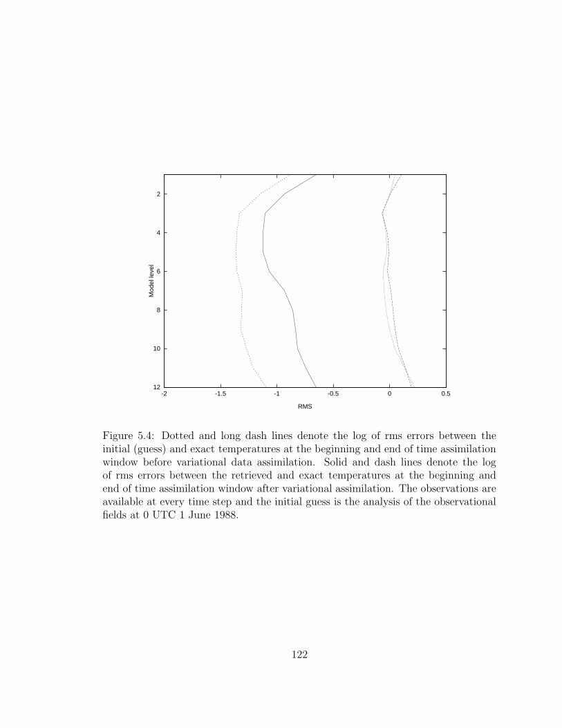
2
4
6
8
10
12-2 -1.5 -1 -0.5 0 0.5
Mod
el le
vel
RMS
Figure 5.4: Dotted and long dash lines denote the log of rms errors between theinitial (guess) and exact temperatures at the beginning and end of time assimilationwindow before variational data assimilation. Solid and dash lines denote the logof rms errors between the retrieved and exact temperatures at the beginning andend of time assimilation window after variational assimilation. The observations areavailable at every time step and the initial guess is the analysis of the observationalfields at 0 UTC 1 June 1988.
122
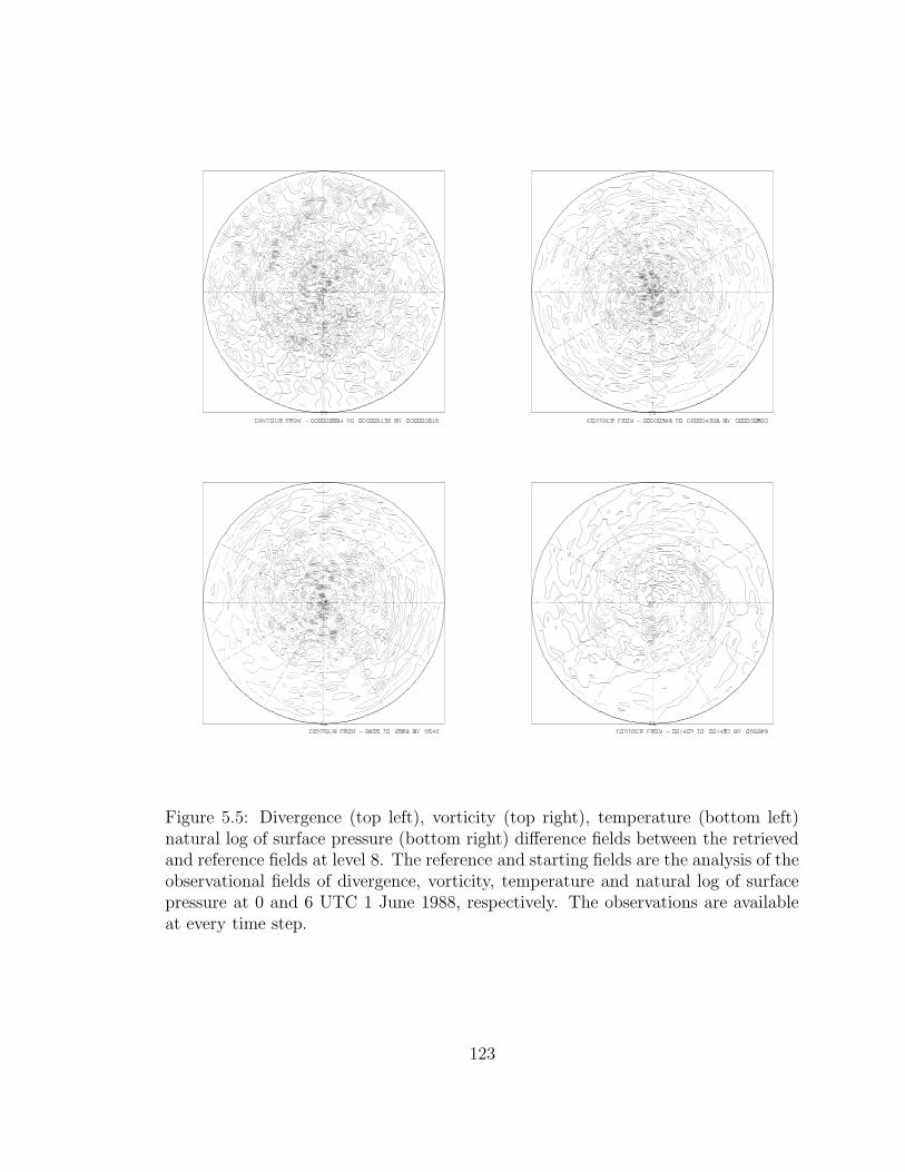
Figure 5.5: Divergence (top left), vorticity (top right), temperature (bottom left)natural log of surface pressure (bottom right) difference fields between the retrievedand reference fields at level 8. The reference and starting fields are the analysis of theobservational fields of divergence, vorticity, temperature and natural log of surfacepressure at 0 and 6 UTC 1 June 1988, respectively. The observations are availableat every time step.
123
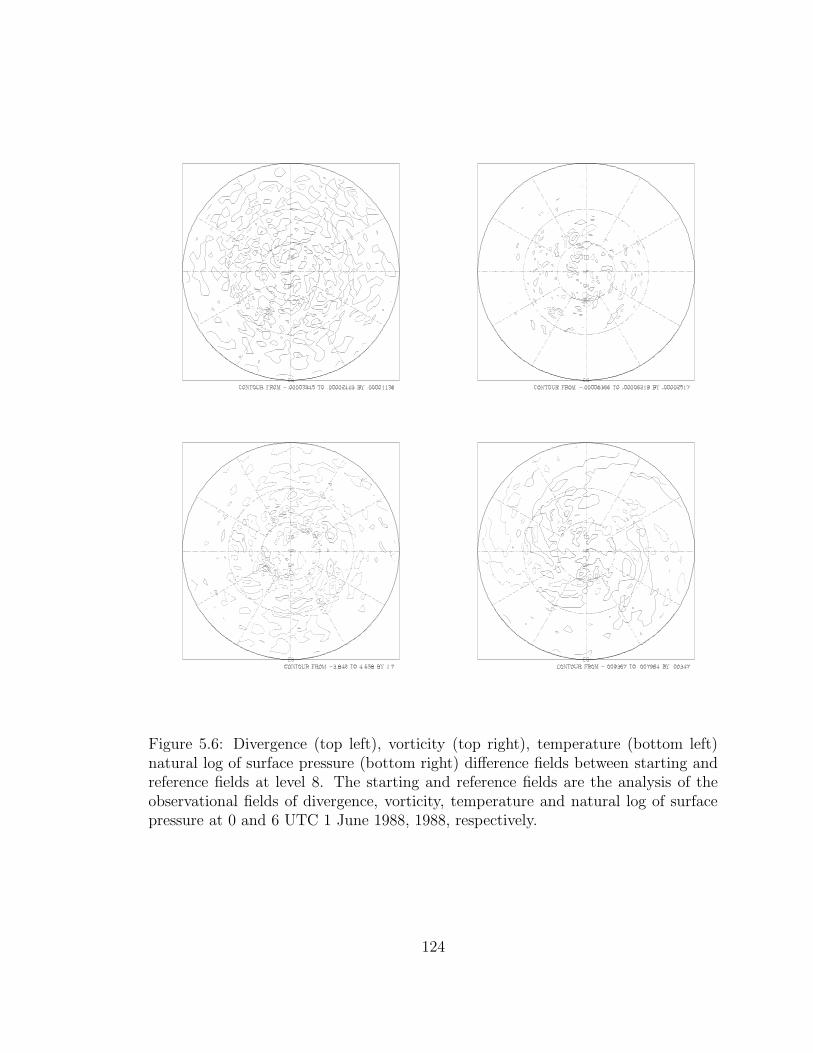
Figure 5.6: Divergence (top left), vorticity (top right), temperature (bottom left)natural log of surface pressure (bottom right) difference fields between starting andreference fields at level 8. The starting and reference fields are the analysis of theobservational fields of divergence, vorticity, temperature and natural log of surfacepressure at 0 and 6 UTC 1 June 1988, 1988, respectively.
124
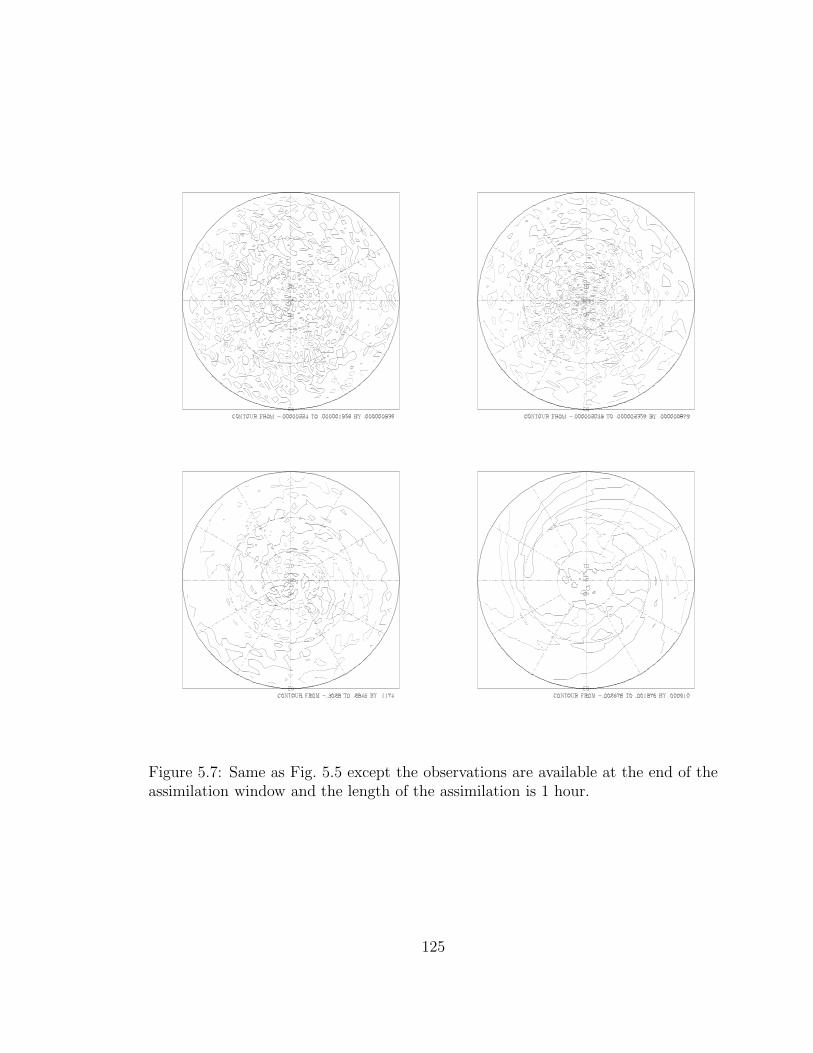
Figure 5.7: Same as Fig. 5.5 except the observations are available at the end of theassimilation window and the length of the assimilation is 1 hour.
125
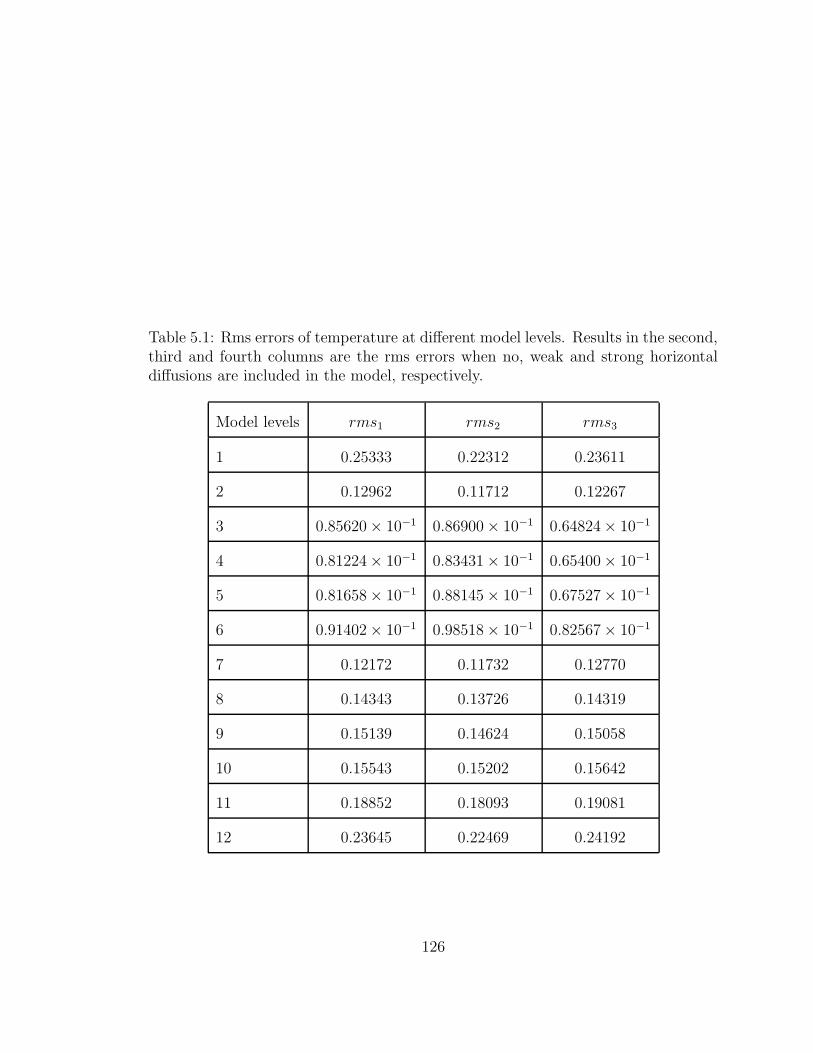
Table 5.1: Rms errors of temperature at different model levels. Results in the second,third and fourth columns are the rms errors when no, weak and strong horizontaldiffusions are included in the model, respectively.
Model levels rms1 rms2 rms3
1 0.25333 0.22312 0.23611
2 0.12962 0.11712 0.12267
3 0.85620 × 10⁻¹ 0.86900 × 10⁻¹ 0.64824 × 10⁻¹
4 0.81224 × 10⁻¹ 0.83431 × 10⁻¹ 0.65400 × 10⁻¹
5 0.81658 × 10⁻¹ 0.88145 × 10⁻¹ 0.67527 × 10⁻¹
6 0.91402 × 10⁻¹ 0.98518 × 10⁻¹ 0.82567 × 10⁻¹
7 0.12172 0.11732 0.12770
8 0.14343 0.13726 0.14319
9 0.15139 0.14624 0.15058
10 0.15543 0.15202 0.15642
11 0.18852 0.18093 0.19081
12 0.23645 0.22469 0.24192
126
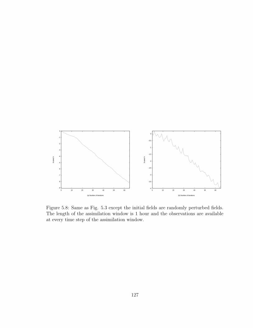
-9
-8
-7
-6
-5
-4
-3
-2
-1
0
0 10 20 30 40 50 60
Sca
led
h
(a) Number of iterations
-4
-3.5
-3
-2.5
-2
-1.5
-1
-0.5
0
0 10 20 30 40 50 60
Sca
led
h
(b) Number of iterations
Figure 5.8: Same as Fig. 5.3 except the initial fields are randomly perturbed fields.The length of the assimilation window is 1 hour and the observations are availableat every time step of the assimilation window.
127
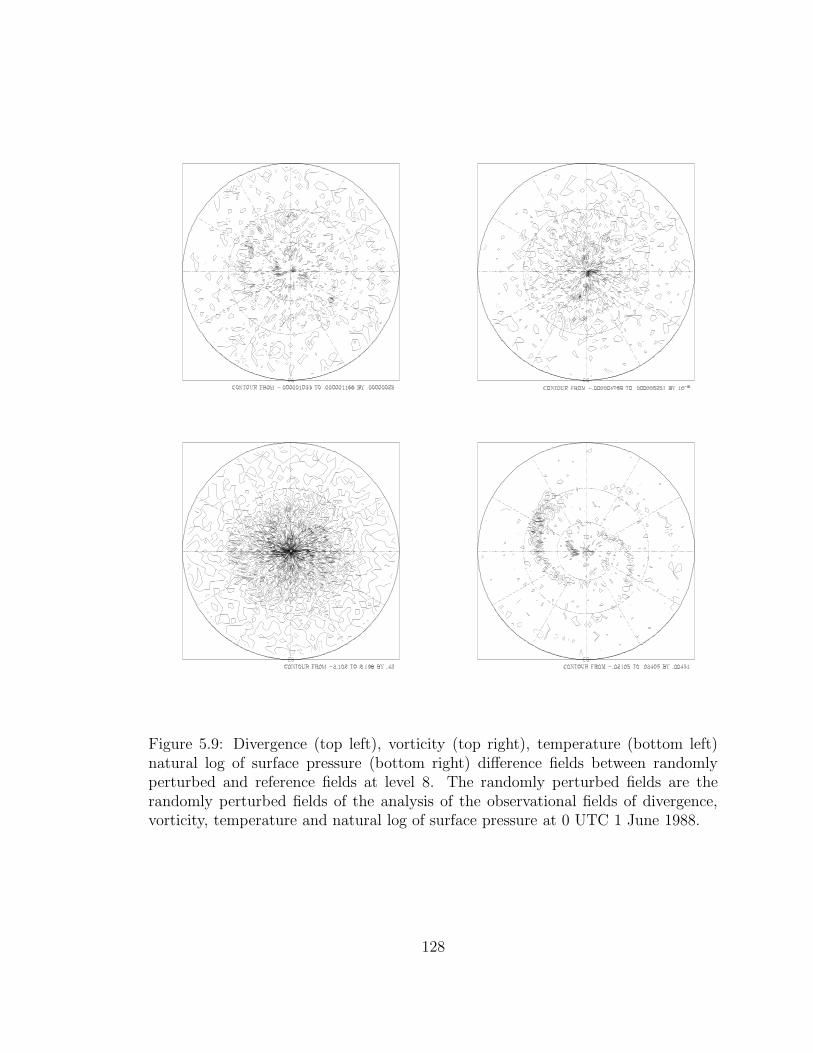
Figure 5.9: Divergence (top left), vorticity (top right), temperature (bottom left)natural log of surface pressure (bottom right) difference fields between randomlyperturbed and reference fields at level 8. The randomly perturbed fields are therandomly perturbed fields of the analysis of the observational fields of divergence,vorticity, temperature and natural log of surface pressure at 0 UTC 1 June 1988.
128
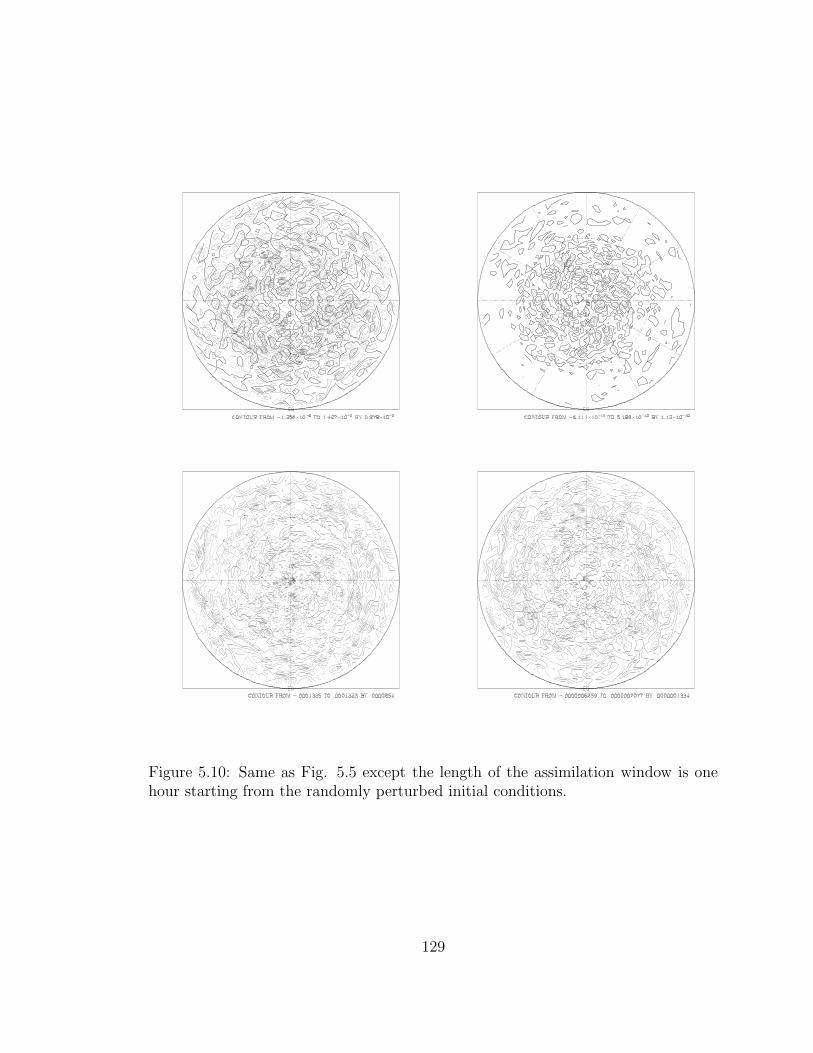
Figure 5.10: Same as Fig. 5.5 except the length of the assimilation window is onehour starting from the randomly perturbed initial conditions.
129
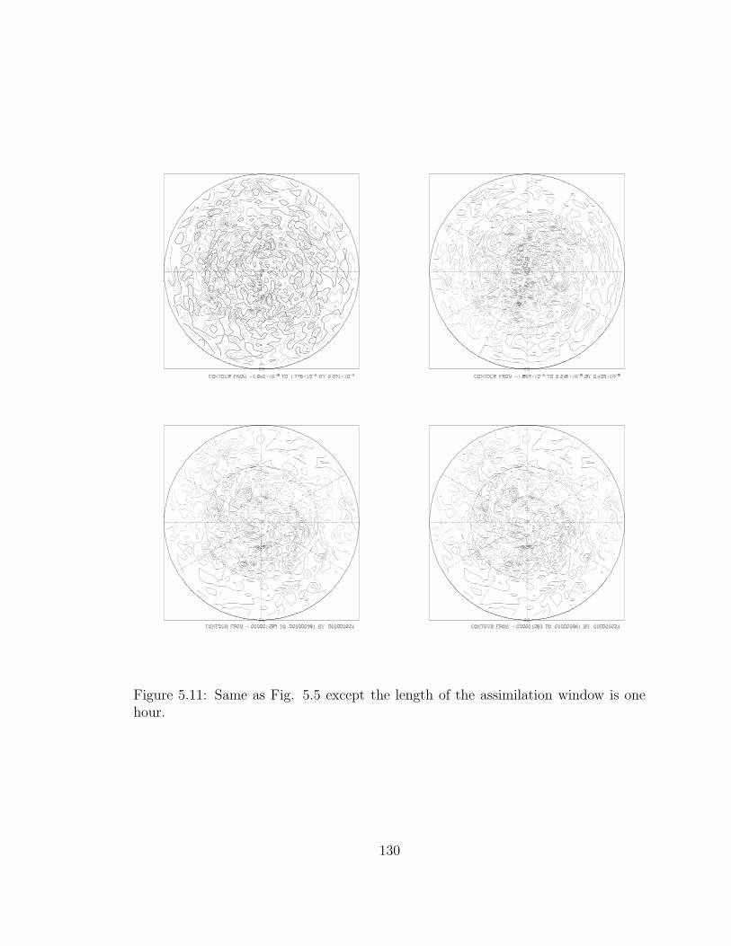
Figure 5.11: Same as Fig. 5.5 except the length of the assimilation window is onehour.
130
Figure 5.12: Same as Fig. 5.5 except the observations are available only at thebeginning and end of assimilation window.
131

Figure 5.13: Same as Fig. 5.3 except the observations are available only at thebeginning and end of assimilation window and the length of the assimilation windowis six hours.
132
Figure 5.14: Same as Fig. 5.4 except The observations are available only at thebeginning and end of the assimilation window.
133
CHAPTER 6
VARIATIONAL NUDGING DATA ASSIMILATION
6.1 Introduction
Among the 4-D data assimilation approaches, variational data assimilation (VDA)
nudging data assimilation (NDA) [195], variational continuous assimilation (VCA)
[52, 235], Kalman-Bucy and extended Kalman-Bucy filtering methods [29, 30, 31, 43,
163, 90, 91, 212] are considered to be five of the most promising techniques capable
of utilizing the ever growing number of asynoptic observations. Briefly, the VDA
method seeks to find an optimal initial condition and /or boundary conditions which
minimizes in the least square sense the differences between the model solution and
observations in a certain assimilation time interval [36, 44, 108, 151, 175, 218, 215].
It uses an optimal control approach based on adjoint model integration to obtain the
gradient of the cost function, with respect to the control variables for the minimization
procedure efficiently [177]. This approach is cheaper than that of using an explicit
finite-difference approximation for the gradient when large-dimensional models are
involved. Nevertheless, the cost of the VDA method for real distributed data is still
prohibitive for operational applications. Additional research is required to improve
the rate of convergence of the minimization part of the algorithm by proper scaling
and weighting as well as developing efficient parallel algorithms for VDA. Other issues
related to VDA concern determining the optimal length of the assimilation window,
the treatment of on-off physical processes such as large-scale precipitation and deep
cumulus convection [9, 231, 237, 216], and the control of high-frequency gravity-wave
oscillations [226, 230], to mention but a few. Moreover, the adjoint VDA method may
also be used to perform parameter estimation and sensitivity analysis.
134
The NDA method relaxes the model state towards the observations during the
assimilation period by adding a non-physical diffusion-type term to the model equa-
tions. The nudging terms are defined as the difference between the observation and
model solution multiplied by a nudging coefficient. The size of this coefficient is cho-
sen by numerical experimentation so as to keep the nudging terms small in comparison
with the dominant forcing terms in the governing equations, in order to avoid the re-
bounding effect that slows down the assimilation process, yet large enough to impact
the simulation. NDA has been successfully used on global scale ([98, 122, 124]) and
in a wide variety of research applications on mesoscale models ([47, 88, 172, 217] etc).
The NDA method can be thought of as an iterative simplified approximation to the
Kalman filter (KF) [119, 122]. The NDA method is a flexible assimilation technique
which is computationally much more economical than the VDA method. However,
results from NDA are quite sensitive to the ad hoc specification of the nudging relax-
ation coefficient, and it is not at all clear how to choose a nudging coefficient so as to
obtain an optimal solution (the theory and examples of NDA are provided in section
6.2).
VCA [52, 235] considers the forecast model error by adding to the right hand sides
of the model equations given by Eq. (1.4) a correction term λφ, i.e. a product of a
prespecified time dependent variable λ and a spatially dependent variable φ,
∂ ~X
∂t= F ( ~X) + λφ. (6.1)
The form of λ controls the distribution of the correction over the assimilation window.
The objective of the VCA technique is to find the optimal φ which minimizes the cost
function. Note that φ contains the same number of degrees of freedom as the initial
state. The VCA is similar to the NDA. However, in the VCA, the correction varies in
time only in a prespecified manner. The correction is calculated to optimally fit the
135
data throughout the assimilation window, rather than relaxing the solution toward
the values at the observation time.
Variational nudging data assimilation (VNDA, which is called optimal nudging
data assimilation in the work of Zou et al. [229]) combines the aforementioned data
assimilation schemes in the most efficient way. The original idea of optimal nudg-
ing data assimilation was put forward by Le Dimet (personal communication). A
parameter-estimation approach is used in the framework of the VDA algorithm to
simultaneously determine the best initial conditions for numerical weather prediction
(NWP) and optimal coefficients for the NDA scheme. The goal is to find the best
initial conditions and optimal nudging coefficients which best assimilate the given
observations. It is well known that the best nudging coefficients are those related
to a KF in a linear system of equations. Applications of the KF technique to the
assimilation of meteorological (or oceanographical) observations has been studied by
several authors [31, 43, 163, 65, 66, 67, 68, 171], and present operational NDA proce-
dures can be described as degraded forms of the KF. However, the KF is very costly
to implement in practice [31, 56]. In Appendix E, the extended KF [163] and the
relationship amongst the KF, VNDA and NDA approaches are described.
We can obtain optimal nudging coefficients in a much more economical way by
using the VDA method in a parameter estimation mode; this allows the adjusting
of variables other than the initial conditions for either linear or nonlinear systems
and employs an adjoint model for gradient calculation. Parameters in the numerical
weather prediction model can easily be incorporated in the adjoint VDA procedure
and serve as additional control variables. The variational algorithm is formulated here
using the nudging coefficients as the control parameters. The nudging coefficients are
estimated so that the model solution is as close as possible to the observations.
In this chapter, we present the results of an application of the VNDA to the
FSUGSM in its full-physics diabatic operational form. The gradient of the cost func-
136
tion with respect to the initial conditions is approximately obtained by integrating
the adjoint model of the adiabatic version of the FSUGSM [219]. This introduces
an error in the gradient calculation but also opens a door for data assimilation of
the most sophisticated forecast models by employing imperfect adjoint models. The
nudging term included in the model equations takes the model error into account.
The nudging term also plays a role in improving the conditioning of the cost function
and thus results in a faster convergence of the minimization process.
The FSUGSM and all its physical processes have been described in Chapter 4
and Appendix F, respectively. In subsections 6.2 and 6.2.3, some simple examples
of the NDA are first presented and then the NDA and VNDA are described for a
general model, respectively. Computational details and numerical results are shown
in section 6.3. A comparison of estimated nudging, optimal nudging and variational
data assimilation is provided in section 6.3.3. Conclusions as well as topics for further
research related to the 4-D VDA with FSUGSM are presented in section 6.4.
6.2 Nudging data assimilation
6.2.1 Some simple examples
In order to get a feeling for the effects of nudging, we consider a few very simple
cases in this subsection.
In NDA there is a preforecast integration period during which model variables are
driven toward the observations by extra forcing terms (nudging terms) in the model
equations. When the actual initial time is reached, the nudging terms are dropped
from the model equations and the forecast proceeds. The principal objective is to
bring the data and the model in harmony and provide a relatively noise-free start
[81]. The schematic representation of the assimilation-forecast cycle of the NDA is
provided in Fig. 6.2.
137
The equations for a particular gridpoint variable α may be expressed in the form
∂α
∂t= F +N(α, t)ε[α(0) − α], (6.2)
where F represents the usual terms in the model equations; N(α, t) is a nonnegative
nudging coefficient; and ε, a positive weight factor ≤ 1, is a confidence factor with
respect to accuracy of the gridpoint value α(0)(t) which is a best estimate based upon
observations. If α(0)(t) is assumed to be the true value, ε would be 1.
First assume that the physical forcing is zero, and further that N is constant and
ε = 1. Then (6.2) reduces to∂α
∂t= N [α(0) − α], (6.3)
or
α = α0e−Nt +Ne−Nt
∫ t
0NeNtα(0)dt, (6.4)
where t = 0 represents the beginning of the preforecast period and α0 is the value of
α at t = 0. If α(0)(t) is assumed to be constant in time toward which α is nudged,
the solution of (6.4) is
α = α(0) + (α0 − α(0))e−Nt. (6.5)
Thus α approaches the observed value α(0) as time passes, though of course never
reaching it in a finite time T .
As a second case assuming the atmosphere and also the observations are changing
linearly with time [i.e., α(0)(t) = α(0)0 + at]. Then the solution for this case is
α = α(0)(t) + [α0 − α(0)0 ]e−Nt − a
N(1 − e−Nt). (6.6)
In this instance it is seen that the initial error, if such exists, is damped toward zero
with increasing time (second term on right-hand side) but the third term approaches
−a/N . Thus at best α approaches the observationally determined value α(0)(t) only
to within the constant a/N , which is the ratio of the rate of change of α(0) to nudging
constant. Also for a large N , the last term will be small.
138
The preceding simple cases have been mainly concerned only with a simple vari-
able rather than a complete system of equations and the physical forcing has been
omitted. In order to treat a more complete system analytically, shallow water equa-
tions with nudging terms added are linearized about a state of rest with constant
Coriolis parameter f and no variation in the y-direction [88]. Assuming periodic
disturbances of the form
X ′ =∑
m
Xm exp(ikmx),
where X ′ is a column vector of the perturbation quantities u′, v′ and h′, km = 2π/Lm,
is the mth wavenumber, Lm is the wavelength and the Xm are the corresponding
amplitudes, the equations for the amplitudes take the form
∂
∂t
um
vm
hm
+
Nu −f ikmg
f Nv 0
ikmH 0 Nh
um
vm
hm
=
Nuu(0)m
Nvv(0)m
Nhh(0)m
(6.7)
or∂X
∂t+ AX = B. (6.8)
Assuming the nudging coefficients and “observations” do not vary in time, the matrix
A and vector B are constants, and the solution is given by a constant vector, A−1B,
and a time-varying part:
X = A−1B +3
∑
j=1
Cje−σj t, (6.9)
where σj are the eigenvalues of A and the Cj are constant vectors that depend on
the initial conditions X(0) and A−1B. The Cj can be determined given X(0) and
X(0) by placing t = 0 in (6.9). In the case where the constant “observations” are in
geostrophic balance, that is, u(0)m = 0 and v(0)
m = (igkm/f)h(0), then X (0) = A−1B;
hence
X −X (0) = C1e−σ1t + C2e
−σ2t + C3e−σ3t, (6.10)
139
Assuming further that the nudging coefficients are all equal to N , Eq. (6.10) leads to
a stationary mode σ1 = N , σ2 = N + iν and σ3 = N− iν, where ν2 = ω2 +f 2. Here ν
is the frequency of inertial gravity waves and ω2 = k2mgH. Thus there is a stationary
mode damped by nudging coefficient and two damped inertial gravity modes with a
resulting approach toward the observational values X (0).
6.2.2 The basic theory of nudging data assimilation
An implicit assumption made in VDA is that the model exactly represents the
state of the atmosphere. However, this assumption is clearly not true because any
numerical model only approximately represents the state of the atmosphere.
The nudging data assimilation (NDA) technique introduced by Anthes [4] consists
in achieving a compromise between the model and observations by considering the
state of the atmosphere to be defined by
∂ ~X
∂t= F ( ~X) +G( ~Xo − ~X), (6.11)
where G is a diagonal matrix with Gq, GT , GD, Gζ and GS as its diagonal sub-
matrix entries representing adjustable nudging coefficients for the surface pressure,
temperature, divergence, vorticity and moisture fields, respectively.
Together with the initial condition
~X(t0) = U, (6.12)
the system (6.11) has an unique solution ~X(U,G).
Let us consider a perturbation U ′ on the initial condition U in Eq. 6.12. The
resulting perturbation on the variable ~X, X is obtained from Eqs. (6.11) and (6.12)
as
∂X
∂t=∂F
∂ ~XX −GX, (6.13)
X(t0) = U ′. (6.14)
140
The main difficulty in the NDA scheme resides in the estimation of the nudging
coefficient G [194]. If G is too large, the fictitious diffusion term will completely dom-
inate the time tendency and will have an effect similar to replacing the model data
by the observations at each time step. Should a particular observation have a large
error that prevents obtaining a dynamic balance, an exact fit to the observation is
not required since it may lead to a false amplification of observational errors. On the
other hand, if G is too small, the observation will have little effect on the solution.
In general, G decreases with increasing observation error, increasing horizontal and
vertical distance separation, and increasing time separation. In the experiment of
Anthes [4] a nudging coefficient of 10−3 was used for all the fields for a hurricane
model and was applied on all the domain of integration. In the experiment of Krish-
namurti et al. [98] the relaxation coefficients for the estimated NDA experiment were
kept invariant both in space and time, and their values were simply determined by
numerical experience. The following values were used:
Gζ , Gq = 10−4s−1 (6.15)
GD = 0.5 × 10⁻⁴s−1,
i.e. the vorticity, divergence and the pressure tendency fields are subjected to the
Newtonian relaxation. The implicit dynamic constraints of the model then spread
the updated information to other variable fields (temperature and moisture fields)
resulting eventually in a set of balanced conditions at the end of the nudging period.
We employ a parameter-estimation approach [8] designed to obtain the best initial
conditions and optimal nudging coefficients G∗ [229]. They are optimal in the sense
that the difference between the model solution and the observations will be small.
The values in (6.16) will be used both as the nudging coefficient for estimated NDA
experiment (usual NDA using ad hoc nudging parameters) and as the initial guess
141
in a variational parameter-estimation approach aimed at obtaining the best initial
conditions and optimal nudging coefficients.
6.2.3 Variational nudging data assimilation
By fitting the model solutions to the observational data, the unknown parameters
of the model can be obtained simultaneously by minimizing a cost function that
measures the misfit between the model results and observations, in which the model
parameters are the control variables along with the initial condition vector in our case
[45, 104, 188]. For example, the barotropic gravity-wave speed in a two-dimension
reduced-gravity, linear-transport model for the equatorial Pacific Ocean was used as
a parameter control variable [193]. In the work of Panchang and O’Brien [159] the
friction coefficient for a one-dimension tidal-flow model was the parameter optimally
estimated from observations. In the work of Lardner et al. [104], the bottom drag
coefficient and depth correction for a two-dimensional hydrodynamical model of the
Arabian Gulf were the parameters optimally estimated.
The application of the variational approach to determine model parameters is
conceptually similar to that of determining the initial conditions. In the following we
will present a brief illustration of the method.
For the VNDA, the cost function J can be defined as
J(U,G) =1
2
M∑
i=0
< W ( ~Xi − ~Xoi ), (
~Xi − ~Xoi ) > + < K(G− G), G− G >, (6.16)
where G denotes the estimated nudging coefficients and the K is specified weighting
matrix. Here observations are assumed to be available everywhere on all model grid
points for simplicity. For a more realistic case, a transform operator C from ~X to ~Xo
should be included in (6.16) and hence G will no longer be a diagonal matrix with
constant terms in each block. The second term plays a double rule. On one hand it
ensures that the new values of the nudging parameters are not too far away from the
142
estimated quantity. On the other hand it enhances the convexity of the cost function
since this term contributes a positive term, K, to the Hessian matrix of J [193].
The solutions of the VNDA procedure can be defined by the best initial condition
U∗ and optimal nudging coefficients G∗ such that
J(U∗, G∗) ≤ J(U,G), ∀G, U. (6.17)
The problem of extracting the dynamical state from observations is now identified as
the mathematical problem of finding initial conditions or external forcing parameters
that minimize the cost function.
Owing to the dynamical coupling of the state variables to the forcing parameters,
the dynamics can be enforced through the use of a Lagrange function constructed by
appending the model equations to the cost function as constraints, thus avoiding the
repeated application of the chain rule when differentiating the cost function. If the
implicit time differencing equations of Eq (6.11) are given by the following equations
~X1 = ~X0 + ∆tF ( ~X0) + ∆tG( ~Xo1 − ~X1), (6.18)
~Xi+1 = ~Xi−1 + 2∆tF ( ~Xi) + 2∆tG( ~Xoi+1 − ~Xi+1), (6.19)
for i = 1, ..., M − 1, then the Lagrange function may be defined by
L = J(U)
+ < P0, ~X1 − ~X0 − ∆tF ( ~X0) − ∆tG( ~Xo1 − ~X1) >
+M−1∑
1
< Pi, ~Xi+1 − ~Xi−1 − 2∆tF ( ~Xi) − 2∆tG( ~Xoi+1 − ~Xi+1), (6.20)
where Pi is a vector of Lagrange multiplies, which are identical to the adjoint model
variables [206]. The Lagrange multiplies are not specified but computed in determin-
ing the best fit. At the minimum point the gradient of the Lagrange function must
be zero. This leads to the following first-order condition:
∂L
∂Xi
= 0, (6.21)
143
∂L
∂Pi
= 0, (6.22)
∂L
∂G= 0, (6.23)
The solution of Eqs (6.21-6.23) is called the stationary point of L. Eq (6.23) results
in (the notation here has some problems)
∇GJ − ∆tP0( ~Xo1 − ~X1)
−M−1∑
1
2∆tPi( ~Xoi+1 − ~Xi+1), (6.24)
which yields the gradient of the cost function with respect to G
∇GJ = ∆tP0( ~Xo1 − ~X1)
+M−1∑
1
2∆tPi( ~Xoi+1 − ~Xi+1), (6.25)
Eq (6.22) recovers discrete form of the original model Eq (6.11), while (6.21) yields
the adjoint equations
PM−1 + 2∆tG∗PM−1 +W ( ~XM − ~XoM) = 0, (6.26)
PM−2 + 2∆tG∗PM−2 − 2∆t( ∂F
∂ ~XM−1
)∗PM−1 +W ( ~XM−1 − ~Xo
M−1) = 0, (6.27)
and
Pi−1 + 2∆tG∗Pi−1 − 2∆t( ∂F
∂ ~Xi
)∗Pi − Pi+1 +W ( ~Xi − ~Xo
i ) = 0, (6.28)
for i = M − 2, M − 3, ..., 1.
As we know from previous chapters, the value of the adjoint variable vector at the
initial time is the gradient of the cost function with respect to the initial conditions
∇UJ = P (t0). (6.29)
Therefore the gradient of the cost function with respect to both the initial conditions
and the nudging coefficients is
∇J = (∇UJ,∇GJ)t. (6.30)
144
Having obtained the value of the cost function J by integrating the model (6.11)
forward, and the value of the gradient by integrating the adjoint Eqs (6.26, 6.27,
6.28) backwards in time, any efficient large-scale unconstrained minimization method
may be employed to minimize the cost function with respect to the vector of control
variables and finally obtain the best initial conditions and an optimal parameter
estimation.
It is worth noting that if G is zero the Eqs (6.26, 6.27, 6.28) reduce to the usual
first order adjoint equations and the VNDA reduces to the VDA. In the case in which
the cost function is defined as an integral, the derivation of the gradient of the cost
function with respect to the nudging coefficients is provided in Appendix D.
6.2.4 Identifiability and stability of parameter estimation
If the parameter estimation is going to be successful, an important question must
be addressed; under what conditions can one expect the proposed estimation method
to yield unique and stable results [22, 23, 24, 104, 153, 159, 193]? Now we discuss
these issues.
Strictly speaking, if the method is going to work, the problem should be well-
posed. The inverse problem is often ill-posed, but there are situations under which
a meaningful solution can be found, although in a limited sense. It will be therefore
important to be able to recognize the circumstances which allow a solution of the
problem to be found. The inverse problem can be defined as follows: let a functional
relationship ~X = f(G) be given between a parameter vector G which in our case is
the nudging coefficients and ~X where ~X represents the state variable of our problem.
The inverse problem will then be to determine the nudging coefficients G on the basis
of ~X and the inverse relationship G = R( ~X). This problem is said to be well-posed
if and only if (1) to every ~X there corresponds a solution G; i.e. a solution exists; (2)
the solution is unique for any given ~X; and (3) the solution depends continuously on
145
~X; i.e. the solution is stable. If the inverse problem fails to satisfy one or more of
these three requirements, it is said to be ill-posed.
Uniqueness and parameter identifiability [93] can be defined in the following way.
Let ~X1 = f(G1) and ~X2 = f(G2) be two solutions of the forward problem, and
G1 = R( ~X1) and G2 = R( ~X2) be two solutions of the inverse problem, then
‖ ~X1 − ~X2‖ = 0 ⇔ ‖G1 −G2‖ = 0, (6.31)
where ‖ · ‖ represents a norm over the appropriate space. In practical problems ~X is
only given at discrete points in space and time, and R represents a minimization of a
functional J as given in previous subsection. While uniqueness refers to the inverse
problem, R, identifiability refers to the forward problem, f . If two sets of parameters
lead to the same function ~X, the parameters are said to be unidentifiable. Uniqueness
on the other hand is concerned with the problem whether different parameters may
be found from a given ~X, if so the parameters are nonunique.
Stability can be defined in the following way. For every ε > 0 there exists a δ such
that for G1 = R( ~X1) and G2 = R( ~X2) one has
‖ ~X1 − ~X2‖ < δ ⇒ ‖G1 −G2‖ < ε. (6.32)
Eq. (6.32) states that small errors in the variables must not lead to large changes in
the computed parameter. Tarantola [203] discusses the concepts of uniqueness and
stability in more detail.
The problems of identifiability and stability can be solved by reducing the number
of parameters to be estimated. In the hydrological literature the most common way
to do this is to approximate the parameters by a known class of functions depending
on a finite number of parameters. If the parameter dimension is not reduced, it may
be difficult or even impossible to determine the spatial structure of the parameter
field. Instability is often characterized by the fact that during the solution process
146
the parameter values are bouncing back and forth between high and low values [193].
Lardner et al. [104] pointed out that in most cases it was necessary to include a term
in the cost function that penalizes large variations in the estimated parameters.
The uniqueness of the solution implies that the cost function J is convex. The
requirement for this condition is that the Hessian matrix is positive definite [73].
Writing the cost function as
J = JU + JG, (6.33)
where JU represents the first term in Eq. (6.16), while JG represents the last term or
the term representing prior information about the parameters (nudging coefficients).
The Hessian is represented by
∂2J
∂G2=∂2JU
∂G2+∂2JG
∂G2. (6.34)
The first term gives
∂2JU
∂G2=
M∑
i=0
< W∂ ~Xi
∂G,∂ ~Xi
∂G> + < W ( ~Xi − ~Xo
i ),∂2 ~Xi
∂G2>, (6.35)
which can be positive or negative. So the first term in the minimization criterion does
not guarantee that the cost function is convex. The last term in Eq. (6.34) gives
∂2JG
∂G2= K, (6.36)
which is clearly a positive term. Adding prior information about the parameters
therefore increases the chance that the cost function will be convex. Of course there
is no guarantee that the term in Eq. (6.36) will make the Hessian positive definite.
Carrera and Neuman [23] discuss the effect of prior information in a few simple
examples of estimation of aquifer parameters. Their examples clearly show that the
addition of prior information leads to unique solutions.
147
6.3 Numerical results of the variational data assimilation
The algorithmic procedure of the VNDA assumes the following form:
1. Set the iteration number k = 0 and initialize the state variable ~X and the
nudging coefficient vector G as U0 and G0, respectively, where G0 is given by
(6.16).
2. Test (Uk, Gk) for convergence. If the following convergence criterion is satisfied
‖Gk‖ ≤ ε‖Uk‖, (6.37)
where ε is a predetermined small number, then stop. Otherwise continue.
3. Integrate the model (6.11) forward in time and calculate the value of the cost
function defined by
J(U,G) =1
2{W < ~Xk(tf ) − ~Xo(tf ), ~Xk(tf ) − ~Xo(tf ) >
+ W < ~Xk(t0) − ~Xo(t0), ~Xk(t0) − ~Xo(t0) >}, (6.38)
if the observations are available only at the beginning and end of the assimila-
tion window , or defined by Eq (6.16) if the observations are available at every
time step.
4. Integrate the adjoint Eqs (6.26, 6.27, 6.28) backwards in time and calculate
the gradient of the cost function with respect to the control variables U and G
using (6.30).
5. Apply the limited-memory quasi-Newton (LBFGS) large-scale unconstrained
minimization algorithm of Liu and Nocedal [117] to obtain a set of new values
for U and G: Uk+1 and Gk+1. Set k = k + 1 and go to step 2.
148

In our experiments, no prior information was presumed (K = 0).
For the nudging terms added to the model, an implicit time-differencing scheme
was used in order to ensure computational stability for any value assumed by the
nudging coefficients. The time integrations are carried out in two steps. The tendency
without the nudging term, ~X∗(t + ∆t), is first calculated. The Newtonian term is
then expressed in finite difference form using the relation
~X(t+ ∆t) − ~X∗(t + ∆t)
2∆t= G[ ~XO(t+ ∆t) − ~X(t+ ∆t)], (6.39)
or
~X(t+ ∆t) =~X∗(t + ∆t) + 2∆tG ~XO(t+ ∆t)
1 + 2∆tG. (6.40)
It is first necessary to obtain the correct gradient of the cost function with respect
to the nudging coefficients in the parameter-estimation procedure before carrying out
the minimization of the cost function. Since otherwise all our calculations will be
erroneous. The Taylor formula applied in the direction G′ = ∇GJ(G) yields
ψ(α) =J(G+ αG′) − J(G)
αG′t · ∇GJ= 1.+O(α‖G′‖). (6.41)
For small α but not too close to the machine accuracy, the value of ψ(α) should
be close to one if the gradient ∇GJ is correctly calculated. Fig. 6.1 indicates that
for α between 10−11 and 10−22 an unit value of φ(α) is obtained and therefore the
correctness of the gradient calculation has been verified.
6.3.1 Variational nudging data assimilation with the adiabatic version of
the FSU global spectral model
Before conducting the VNDA with the FSUGSM in its full-physics operational
form, it is important to ensure that the VNDA performs successfully with the adia-
batic version of the FSUGSM since the adjoint model is derived from the adiabatic
149
version of the FSUGSM. As stated previously, the gradient calculation is exact except
for computational errors.
The experiments are devised as follows: the model-generated values starting from
an analysis of the real observational data at 6 UTC 1 June 1988 are used as obser-
vations and the initial guess for initial conditions is taken as an analysis of the real
observational data at 0 UTC 1 June 1988. The initial guess for nudging coefficients
is given by (6.16).
The experiments carried out here involved nudging the surface pressure, diver-
gence and vorticity. Figs. 6.6 (dash line) and 6.4 display the variations of the log
of the scaled cost function (Jk/J0) and scaled gradient norm (‖~gk‖/‖~g0‖) with the
number of iterations in the minimization process when the observations are available
at every time step and only at the beginning and end of the assimilation window,
respectively. After either 24 or 18 iterations, the normalized cost function and the
normalized norm of the gradient are reduced by more than 2.5 and 2 orders of mag-
nitude, respectively, irrespective which set of observations is used. At this stage the
prescribed convergence criterion given by (6.37) with ε = 10−5 is satisfied. In the case
where the observations are available at every time step of the assimilation window,
by continuing the minimization process, the scaled cost function and scaled gradient
norm decreased another 2 and 1 orders of magnitude after 65 iterations, respectively.
Both the cost function and the gradient norm continue to decrease even after 65
iterations. We note that due to the nudging effect, it appears that when more obser-
vations are added, the convergence rate becomes faster. The opposite is true for the
VDA experiments carried out in Chapter 5. Comparing Figs. 6.6 and 6.4 with Figs.
5.3 and 5.13, it is observed that the VNDA is indeed much faster than the VDA for
our test problem. In both of VNDA experiments the minimization requires less than
25 iteration to satisfy the prescribed convergent criterion while the minimizations
requires more than 65 iterations to converge in both of the VDA experiments. This
150
is due to the fact that the conditioning of the Hessian is improved when a nudging
term is added to the forecast model. These figures indicate that VNDA yields higher
quality solutions requiring much less iterations. If we notice that the only additional
cost for VNDA is three more control variables (nudging coefficients) and the calcula-
tion of the gradient of the cost function with respect to these variables, the VNDA is
really cost effective in obtaining a speed up of the convergence of the minimization
process.
It is a good idea to consider the difference fields between the retrieved fields
and the observation fields before and after the minimization process, since these
difference fields measure the ability of the VNDA to retrieve the observational fields.
Figs. 6.8 and 6.5 show the difference fields between the retrieved fields of divergence,
vorticity, temperature and natural log of the surface pressure and the corresponding
reference (observational) fields at the beginning of the assimilation window after the
minimization process for the two experiments. Comparing with the same difference
fields (Fig. 5.6) before the minimization process, it is observed that after minimization
the maximum difference values are reduced by one order of magnitude in all difference
fields of divergence, vorticity, temperature and natural log of the surface pressure in
both cases.
Figs. 6.3 and 6.7 display the evolution of the nudging coefficients, Gln p, Gζ and
GD, in the VNDA procedure. During the first 15 iterations, all the nudging coefficients
experience a dramatic increase for both cases. After 15 iterations the increases level-
off. The optimal values of the nudging coefficients are provided in Table 6.1.
It is observed that the optimal nudging coefficients are two orders of magnitude
bigger than the initial guesses given by (6.16), which were suggested by Krishnamurti
et al. [98]. By noticing that the horizontal truncation of our experiment (T42) is
smaller than theirs (T106), the values obtained appear to be very reasonable since it
151
is general experience that the nudging coefficients increase with decreasing horizontal
resolution.
We note here that the optimal nudging coefficients do not tend to infinity as the
minimization proceeds. This is due to the fact that when the minimization process
proceeds, both the initial state U and the nudging coefficients G are updated and the
optimal solution of the minimization problem is obtained due to the combined effect
of the model dynamics and the nudging term.
We also carried out an experiment starting from the randomly perturbed initial
conditions described in section 5.4.2 with the observations available at every time
step. The results are similar to the results described above and are displayed in Figs.
6.9, 6.10 and 6.11.
All previous experiments were carried out starting from an analysis of the obser-
vational fields of divergence, vorticity, temperature and natural log of surface pressure
at 0 UTC 1 June 1988. These analysis fields are not initialized. One may assume the
existence of spurious gravity waves (high frequency “noise”) in them. The nonlinear
normal mode initialization (NNMI) permits an explicit filtering of the unwanted high
frequency oscillations (implied by the initial data) consistent with the framework of
the particular dynamical prediction model being used. Therefore, in order to inves-
tigate the impact of gravity oscillations on the VNDA, we apply the NNMI to the
above analysis fields and perform the same experiments starting from the resulting
fields of the NNMI. The results are similar to the results described above. Fig. 6.6
(solid lines) shows the results of VNDA when the observations are available at every
time step of the assimilation window. It is clear that there are no sizable differences
whether the VNDA starts from either the analysis of the observational fields or from
the fields initialized by the NNMI, which means there are almost no spurious gravity
waves in the analysis of the observational fields.
152
6.3.2 Variational nudging data assimilation with the FSU global spectral
model in its full-physics operational form
In this subsection, we will apply the VNDA to the FSUGSM in its full-physics
operational form while using the same adjoint model of the adiabatic version of the
FSUGSM to calculate the gradient of the cost function. An implicit assumption
made here is that the gradient of the cost function thus calculated is a reasonable
approximation to the exact gradient such that the VNDA could proceed successfully.
The same experiments as described in subsection 6.3.1 are performed when ob-
servations are available at every time step and only at the beginning and end of the
assimilation window, respectively. In Fig. 6.12 the cost function and the gradient
norm are shown as functions of the number of iterations for all the experiments. The
values of the cost function and gradient norm are normalized by their initial values,
respectively. After 9 iterations the cost function and gradient norm are reduced by
more than 1.8 and 1.7 orders of magnitude, respectively, in the case where obser-
vations are available at every time step of the assimilation window. Based on the
behaviour of the gradient norm and the cost function, the minimization is satisfac-
tory, i.e. the cost function and gradient norm do not decrease significantly after 8
iterations.
In all aforementioned assimilation experiments we have also calculated the cost
functions corresponding to each variable (divergence, vorticity, temperature and pres-
sure). It is noticed that the decreases of the different components of the cost function
are uniform and similar to the decrease in the total cost function.
The nudging coefficients as a function of the number of iterations from the present
experiment are shown in Fig. 6.13. The optimal nudging coefficients obtained in this
case are Gln p = 0.9553 × 10⁻³, Gζ = 0.6081 × 10⁻² and GD = 0.3159 × 10⁻². They
are very similar to the corresponding optimal nudging coefficients obtained in the
previous subsection. The behavior of the nudging coefficients as a function of the
153
number of iterations is also very similar in all the experiments performed in this
thesis.
It is important to note that, even though an approximate gradient is used in the
minimization, the VNDA works successfully. This may lead to a possible operational
implementation of the 4-D VDA for sophisticated operational models while using a
simplified adjoint model to calculate the gradient. If full adjoint models of the most
complex models in their full-physics operational form were used, the convergence rate
would be improved and the minimum would be different from that obtained using
simplified adjoint models. But it is reasonable to assume that they will not be far
from each other. All these results indicate that the assumption mentioned at the
beginning of this subsection seems to be very reasonable. Courtier et al. [37] and
Zupanski [235] also employed simplified adjoint models to obtain the gradient of the
cost function with respect to control variables while integrating the nonlinear model
in its full-physics operational form. Their results agree with ours.
The moisture field is not part of the control variables vector in the present ex-
periment. Only divergence, vorticity, temperature and natural log of surface pressure
fields are updated explicitly during each iteration of the minimization process. The
moisture field is implicitly updated through the forecast model integrations, i.e. the
impact of the improved fields of divergence, vorticity, temperature and natural log of
surface pressure progressively propagates to the moisture field through the forward
model integrations.
154
6.3.3 Comparisons of estimated nudging, optimal nudging and variational
data assimilation
In this section we compare the NDA and VNDA techniques when observations are
available at every time step of the assimilation window. The FSUGSM is used in its
full-physics operational form. The basic experiments that follow consist of four types
of assimilation:
1. A control assimilation without nudging,
2. An assimilation with estimated nudging coefficients as suggested by Krishna-
murti et al. [98],
3. An assimilation with optimal nudging coefficients obtained in subsection 6.3.2
by an optimal parameter-estimation procedure using the adjoint technique,
4. VNDA minimizing a cost function measuring the distance between the model
solution and observations. An overview of the aforementioned assimilations are
displayed in Fig. 6.2.
With the estimated and optimal nudging coefficients we may carry out two parallel
NDAs. For the sake of comparison, and with a view to obtain a better insight into the
ability of the VNDA procedure, we also carried out a similar VNDA experiment. The
ensuing 12 hour integrations from the retrieval are used for carrying out a comparison
with the corresponding results of NDA schemes.
We do not intend to compare the NDA with the VNDA approaches directly since
the two models have their own arbitrariness in the definition of the cost function, the
choice of the minimization algorithm, the determination of the stopping criteria, the
length of assimilation window and the choice of nudging coefficients. However, the
ability to reconstruct as accurately and economically as possible the state of the flow
is of paramount importance.
155
Rms errors are computed for the aforementioned assimilation experiments. Dis-
tributions of the rms differences for temperature fields between true solution and the
forecast at the end of the forecast period are displayed in Figs. 6.14, respectively.
As expected [229], the NDA with estimated nudging coefficients yields the poorest
results while the VNDA yields the best results.
6.4 Conclusions
In this chapter we took advantage of the VDA’s ability to perform an optimal
parameter estimation to obtain both optimal nudging coefficients and the best initial
conditions simultaneously. That is the nudging coefficients are part of the control
variables vector. Both the initial conditions and the nudging coefficients are updated
after each iteration of the minimization process. Since at every iteration the model
integration is carried out with current estimated nudging coefficients used in the
nudging term, the conditioning of the Hessian is improved. Thus variational nudg-
ing assimilation results in faster convergence rate compared with the 4-D VDA. The
resulting optimal nudging coefficients can be applied in NDA, thus the term optimal
NDA. The optimal NDA is practically implementable and performs very well in as
far as the convergence and quality of the resulting assimilation state are concerned.
This procedure is much more economical than the VDA approach due to tremendous
computational cost of the VDA. Therefore the optimal NDA is also a good candidate
as a future data assimilation scheme where the observations in a certain period of time
can be effectively incorporated into the model so as to obtain the best initial condi-
tions. The relationship amongst the KF, VNDA and NDA approaches is described in
Appendix E, can also be found in reference [229].
In subsection 6.3.2, we carried out VNDA experiments using the FSUGSM in its
full-physics operational form and using a simplified adjoint model of the adiabatic
156
version of the FSUGSM to calculate the gradient approximately. The results thus
obtained are realistic and both the cost function and the gradient norm in all experi-
ments show sufficient decreases. Although the moisture field is not explicitly updated,
the resulting moisture field from VNDA is satisfactory. The main conclusion of this
chapter is that the VNDA could be performed successfully using most sophisticated
models while using a simplified adjoint model to calculate the gradient.
It might be desirable for nudging coefficients G varying both in time as well as
over the horizontal domain and on the different vertical levels. Zou et al. [229]
demonstrated the ability of the VNDA to obtain optimal nudging coefficients varying
in space in the framework of a parameter-estimation approach. In their experiment,
the spatial variability of the optimal nudging coefficients is very small. Therefore,
using constant optimal nudging coefficients for each variable is satisfactory for perfect
observations’ assimilation. When the nudging coefficients have too many degrees of
freedom, physical constraints should be added to the choice of the nudging coefficients.
We will pay special attention to this topics in the future.
157
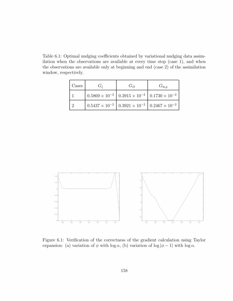
Table 6.1: Optimal nudging coefficients obtained by variational nudging data assim-ilation when the observations are available at every time step (case 1), and whenthe observations are available only at beginning and end (case 2) of the assimilationwindow, respectively.
Cases Gζ GD Gln p
1 0.5869 × 10⁻² 0.3915 × 10⁻² 0.1730 × 10⁻²
2 0.5437 × 10⁻² 0.3921 × 10⁻² 0.2467 × 10⁻²
0
0.2
0.4
0.6
0.8
1
1.2
1.4
-22 -20 -18 -16 -14 -12 -10
-6
-5
-4
-3
-2
-1
0
-22 -20 -18 -16 -14 -12 -10
Figure 6.1: Verification of the correctness of the gradient calculation using Taylorexpansion: (a) variation of φ with logα, (b) variation of log |φ− 1| with logα.
158
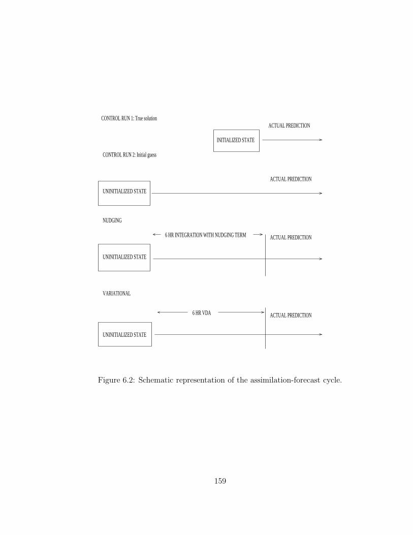
CONTROL RUN 2: Initial guess
UNINITIALIZED STATE
UNINITIALIZED STATE
UNINITIALIZED STATE
ACTUAL PREDICTION
ACTUAL PREDICTION
ACTUAL PREDICTION
ACTUAL PREDICTION
INITIALIZED STATE
6 HR VDA
6 HR INTEGRATION WITH NUDGING TERM
NUDGING
VARIATIONAL
CONTROL RUN 1: True solution
Figure 6.2: Schematic representation of the assimilation-forecast cycle.
159
Figure 6.3: Variation of the nudging coefficients, Gln p (dash line), Gζ (solid line) andGD (long dash line), with the number of iterations. Both the initial conditions andthe nudging coefficients Gln p, Gζ and GD serve as control variables. The observationsare available only at the beginning and end of the assimilation window.
160
Figure 6.4: Variation of the log of the scaled cost function (Jk/J0) and the scaledgradient norm (‖~gk‖/‖~g0‖) with the number of iterations using LBFGS algorithm.The observations are available only at the beginning and the end of the assimilationwindow.
161
Figure 6.5: Divergence (top left), vorticity (top right), temperature (bottom left) andnatural log of surface pressure (bottom right) difference fields between the retrievedfields and the reference fields at level 8. The starting fields are the analysis fieldsof divergence, vorticity, temperature and natural log of surface pressure at 0 UTC 1June 1988. Both the initial conditions and the nudging coefficients Gln p, Gζ and GD
serve as control variables. The observations are available only at the beginning andend of the assimilation window.
162
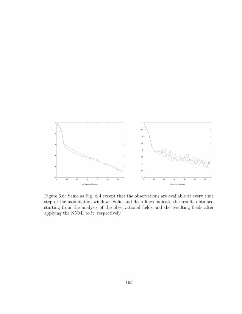
-5
-4
-3
-2
-1
0
0 10 20 30 40 50 60
(a) Number of iterations
-4
-3.5
-3
-2.5
-2
-1.5
-1
-0.5
0
0 10 20 30 40 50 60
(b) Number of iterations
Figure 6.6: Same as Fig. 6.4 except that the observations are available at every timestep of the assimilation window. Solid and dash lines indicate the results obtainedstarting from the analysis of the observational fields and the resulting fields afterapplying the NNMI to it, respectively.
163
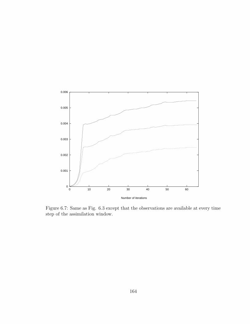
0
0.001
0.002
0.003
0.004
0.005
0.006
0 10 20 30 40 50 60
Number of iterations
Figure 6.7: Same as Fig. 6.3 except that the observations are available at every timestep of the assimilation window.
164
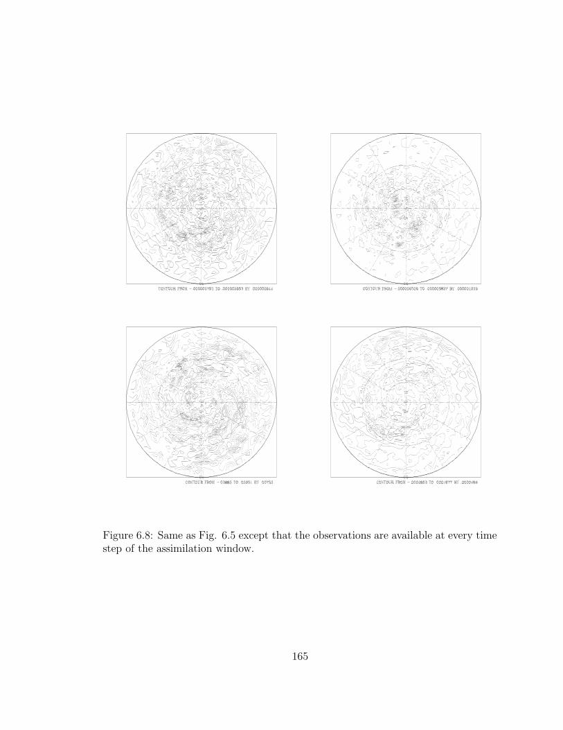
Figure 6.8: Same as Fig. 6.5 except that the observations are available at every timestep of the assimilation window.
165
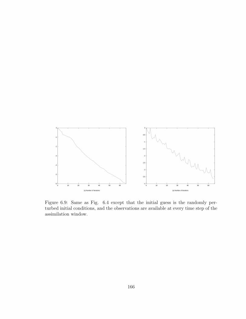
-6
-5
-4
-3
-2
-1
0
0 10 20 30 40 50 60
(a) Number of iterations
-4
-3.5
-3
-2.5
-2
-1.5
-1
-0.5
0
0 10 20 30 40 50 60
(a) Number of iterations
Figure 6.9: Same as Fig. 6.4 except that the initial guess is the randomly per-turbed initial conditions, and the observations are available at every time step of theassimilation window.
166
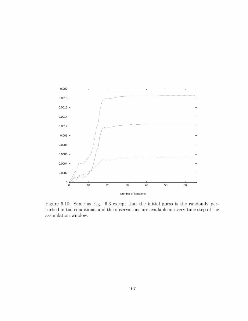
0
0.0002
0.0004
0.0006
0.0008
0.001
0.0012
0.0014
0.0016
0.0018
0.002
0 10 20 30 40 50 60
Number of iterations
Figure 6.10: Same as Fig. 6.3 except that the initial guess is the randomly per-turbed initial conditions, and the observations are available at every time step of theassimilation window.
167
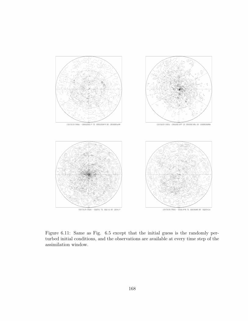
Figure 6.11: Same as Fig. 6.5 except that the initial guess is the randomly per-turbed initial conditions, and the observations are available at every time step of theassimilation window.
168
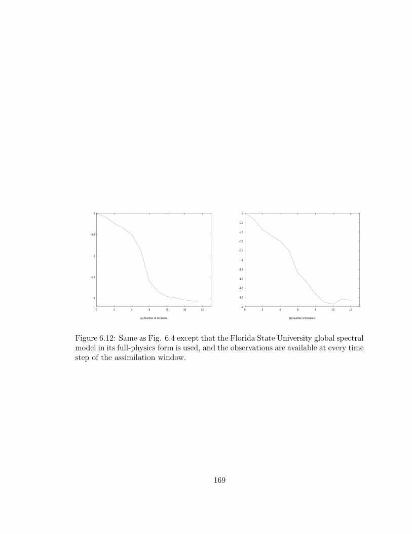
-2
-1.5
-1
-0.5
0
0 2 4 6 8 10 12
(a) Number of iterations
-2
-1.8
-1.6
-1.4
-1.2
-1
-0.8
-0.6
-0.4
-0.2
0
0 2 4 6 8 10 12
(b) Number of iterations
Figure 6.12: Same as Fig. 6.4 except that the Florida State University global spectralmodel in its full-physics form is used, and the observations are available at every timestep of the assimilation window.
169
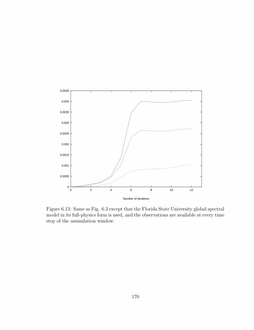
0
0.0005
0.001
0.0015
0.002
0.0025
0.003
0.0035
0.004
0.0045
0 2 4 6 8 10 12
Number of iterations
Figure 6.13: Same as Fig. 6.3 except that the Florida State University global spectralmodel in its full-physics form is used, and the observations are available at every timestep of the assimilation window.
170
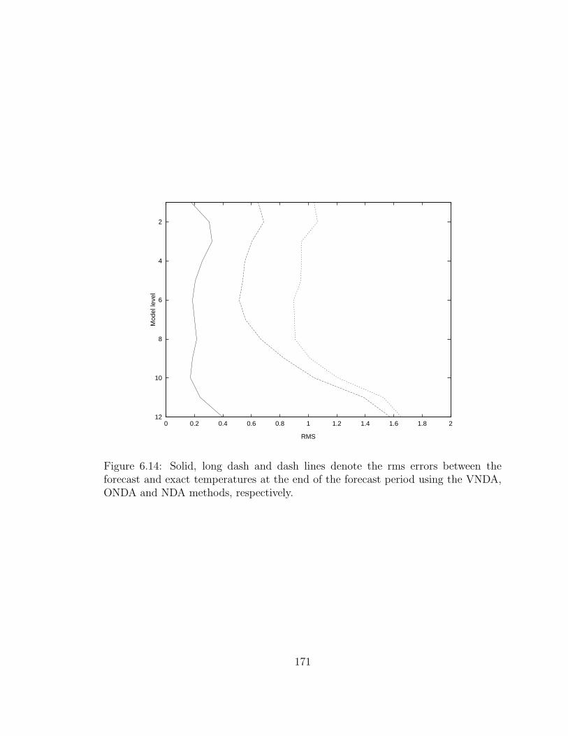
2
4
6
8
10
120 0.2 0.4 0.6 0.8 1 1.2 1.4 1.6 1.8 2
Mod
el le
vel
RMS
Figure 6.14: Solid, long dash and dash lines denote the rms errors between theforecast and exact temperatures at the end of the forecast period using the VNDA,ONDA and NDA methods, respectively.
171
CHAPTER 7
SUMMARY AND CONCLUSIONS
In this thesis, we have systematically studied 4-D VDA applied to numerical
weather prediction problems, i.e. solving the problems related to finding the best ini-
tial conditions such that the sum of weighted squares of the difference between model
solution and the observations is minimized over a period of time. The 4-D VDA
uses iterative large-scale unconstrained minimization algorithms in the framework of
optimal control theory of PDEs to iteratively find aforementioned best initial condi-
tions to a forecast model. Each iteration of the minimization algorithm requires the
calculation of the gradient of the cost function with respect to the control variables.
Theoretically, this gradient could be calculated by finite-difference approximation or
automatic differentiation. But these approaches are too costly. Here the gradient of
the cost function with respect to the control variables is found by integrating a first
order adjoint model backwards in time from the final time to the initial time of the
assimilation window while introducing the weighted differences between the model
solution and the observations into the adjoint model whenever the observations are
available. This gradient is then used to find a descent direction along which the cost
function could be reduced. A step size will be calculated such that a maximum re-
duction in the cost function in the descent direction is obtained. From the step size
and the descent direction, the approximate initial conditions to the forecast model are
updated and the process of determining the gradient, descent direction, step size and
the updated initial conditions is repeated until the minimization algorithm converges,
i.e. satisfies a prescribed convergence criterion. The updated initial conditions at the
172
end of iterative minimization procedure are the best initial conditions minimizing the
cost functional, while satisfying the forecast model equations as a strong constraint.
In Chapters 2 and 3, the thesis focuses on the analysis of the minimization pro-
cess and the improvement of large-scale unconstrained minimization algorithms. Since
these issues are strongly related to the structure of the Hessian of the cost function, a
SOA theory is developed and applied to a shallow water equations model. The SOA
model is similar to the FOA model in form (see Fig. 2.1). Given a perturbation vector
U ′ on the initial condition vector U , the Hessian (H) vector product HU ′ is obtained
by integrating the SOA model backwards in time from the final time to the initial time
of the assimilation window while introducing the first order adjoint variables and the
weighted tangent linear variables into the SOA model at each time step. Comparing
with the finite-difference scheme (3.19), the above adjoint Hessian/vector calculation
strategy yields a more accurate Hessian/vector product since it does not require the
user to select a finite-difference parameter h as the finite-difference scheme does. The
numerical cost of using the SOA approach is roughly the same as that of using the
finite-difference approach, i.e. both approaches require four model integrations and
the numerical cost of each model integration is approximately the same as any other
model integrations. There are many applications of the SOA approach in calculating
the Hessian/vector product. In this thesis, we applied the SOA approach to (a) the
calculation of eigenvalues of the Hessian; (b) the calculation of the sensitivity of the
cost function with respect to observational errors; (c) the implementation of the large-
scale truncated Newton method [134] using a two dimensional limited-area shallow
water equations model. The results presented here demonstrate that (a) the power
method can be efficiently implemented to obtain estimates of the eigenvalues and the
condition numbers of the Hessian matrix with the matrix/vector product calculated
using SOA approach. The variation of the extremal eigenvalues with the number of
the iterations indicates that most changes of the largest eigenvalue occur during the
173
first few iterations of the minimization procedure, which might explain why most of
large-scale features are reconstructed earlier than the small scale features in the VDA
retrieval solution during the minimization process [149]. The fact that the smallest
eigenvalues of the Hessians of the cost function remain positive during the minimiza-
tion process indicates the uniqueness of the optimal solution; (b) the sensitivity of
the cost function with respect to observational errors depends on the time when the
errors occur, the specific field containing the errors, and the spatial location where
the errors occur. The cost function is more sensitive to the observational errors occur-
ring at the beginning of the assimilation window, to errors in the geopotential field,
and to errors at these grid point locations where intensive events occur; (c) although
the ATN algorithm and TN algorithm of Nash [134] differ from each other only in
the use of a more accurate Hessian/vector product for carrying out the large-scale
unconstrained optimization required in VDA, the ATN algorithm yields results which
are twice as fast as these obtained by the TN algorithm both in terms of number of
iterations (i.e. convergence rate) as well as in terms of CPU time. Further the ATN
algorithm turns out to be faster than the LBFGS method in terms of CPU time for
the problem tested.
In Chapter 4 we described the FSUGSM in both physical and spectral spaces, its
semi-implicit time differencing algorithm and its vertical discretization. In Chapter
5, the TLM and FOA models of the FSUGSM were first developed and then were
verified for their correctness. The FOA model was then used to obtain the gradient
of the cost function with respect to the control variables. The correctness of the
calculation of this gradient was verified by using a Taylor expansion. Finally, we
conducted a series of experiments to demonstrate the numerical feasibility of 4-D
variational data assimilation with the FSUGSM. The 4- VDA in this chapter starts
from two types of initial conditions: an analysis of the real observational data and a
randomly perturbed initial condition of the above analysis. It is demonstrated that
174
the VDA performs successfully with different scenarios of observations distributed in
time irrespective which type of initial conditions is used. The impact of observations
being available at the beginning of the assimilation window is dramatic in so far as
the decrease of the cost function is concerned since information on the entire field is in
effect available. When observations are available both at the beginning and the end of
the assimilation window, adding more observations in the middle of the assimilation
window has only a weak impact on the convergence rate of the minimization process.
It is also demonstrated that the presence of horizontal diffusion in the model yields
a more accurate solution to the variational data-assimilation problem.
In Chapter 6, the model forecast error is considered by adding a non-physical
diffusion-type term (i.e. the nudging term) to the model equations. The magnitude
of this nudging term is also optimally estimated in the process of the minimization
of a cost functional. We took advantage of the VDA’s ability to perform optimal
parameter estimation to obtain both optimal nudging coefficients and the best initial
conditions simultaneously, i.e. the nudging coefficients are part of the control variables
vector. Both the initial conditions and the nudging coefficients are updated after each
iteration of the minimization process. Since at every minimization iteration a model
integration has to be carried out with current estimated nudging coefficients used
in the nudging term, the conditioning of the the Hessian matrix is improved. Thus
variational nudging assimilation results in a faster convergence rate compared with
4-D VDA. The resulting optimal nudging coefficients are applied in the NDA, thus
the term optimal NDA. The optimal NDA is practically implementable and performs
very well in as far as the convergence and quality of the resulting assimilation state
are concerned. This procedure is much more economical than the VDA owing to the
tremendous computational cost of the VDA. Therefore the optimal NDA constitutes
a good candidate for future data assimilation schemes where observations in a certain
time window can be effectively incorporated into the model so as to obtain the best
175
initial conditions, i.e. physical initialization. Zou et al. [229] proved this method to
be related to the KF method.
In subsection 6.3.2, we carried out VNDA experiments using the FSUGSM in its
full-physics operational form and using a simplified adjoint model of the adiabatic
version of the FSUGSM to calculate the gradient approximately. The results thus
obtained are realistic and both the cost function and gradient norm in all experiments
show a sufficient decrease. When the physical processes are included in forecast
models, the numerical cost of model integration increases dramatically. Calculation
of the gradient of function using a simplified model reduces the computational cost
of the 4-D VDA at the cost of an error in the gradient. The main conclusion of this
chapter is that the VNDA could be performed successfully using most sophisticated
models while using a simplified adjoint model to calculate the gradient.
The VNDA converges faster than the VDA. It is also easy to implement. But
the numerical cost is still prohibitive for operational implementation of the method.
Preconditioning is an alternative to speed up the minimization process, but it is not
easy to implement in practice. Due to the large dimension and high nonlinearity
of the VDA problems, it is only possible to improve the conditioning to a limited
extent. Therefore it is important to study new ways to formulate the problem and
new algorithms to perform the minimization. Courtier et al. [37] has proposed to
update the perturbations on the basic state instead of updating the state variable
itself (incremental approach). It should be pointed out that the evolution of the per-
turbations is approximately described by the TLM. Thus the formulation is not exact.
But it might be scientifically acceptable. To develop new algorithms, one should con-
sider how to implement Newton’s algorithm in the VDA. Newton’s algorithm has a
quadratic convergence rate. Thus it might be the only algorithm which could lead
to operational implementation of the 4-D VDA before a generation of significantly
faster high performance parallel computers being developed.
176
Developing high performance parallel computing algorithms is another alternative
[21, 150]. For instance, in the adjoint truncated Newton algorithm, there are four
model equations involved, namely, nonlinear model integration, TLM integration,
FOA model integration and SOA model integration. Once the basic model integration
is carried out, the TLM integration and FOA model integration can be carried out
in a parallel manner. This strategy will improve the efficiency of the ATN algorithm.
It is also possible to partition the computational domain into subdomains (domain
decomposition) and carry out the VDA in each subdomain in parallel [21, 150], both
for the forward nonlinear model as well as for the linear adjoint model.
177
APPENDIX A
A SIMPLE EXAMPLE WITH EXACT SOLUTIONS
In this appendix we will illustrate the whole process of using adjoint model tech-
niques in the 4-dimensional data assimilation by presenting a very simple linear exam-
ple. Because the example has exact solutions for the model equation, TLM, FOA and
SOA models, the theory introduced in the Chapters 1 and 2 will be clearly illustrated.
Let us consider the following 1-dimensional model equation
∂X
∂t= −X, (A.1)
X(0) = U, (A.2)
where the time t runs from 0 to 1. Using a direct integration the solution of the model
can be obtained as
X = Ue−t. (A.3)
Let us further suppose that the observations are model generated with the initial
condition
X(0) = 1, (A.4)
then from Eq. (A.3), the observation may be written as
Xo = e−t. (A.5)
Let us define the cost function as
J(U) =1
2
∫ 1
0< (X −Xo), (X −Xo) > dt, (A.6)
then
J(U) =(U − 1)2
4(1 − e−2). (A.7)
178
The first order adjoint model of Eqs. (A.1) and (A.2) may be written as
−∂P∂t
= −P + (X −Xo), (A.8)
i. e.
−∂P∂t
= −P + (U − 1)e−t, (A.9)
P (1) = 0, (A.10)
where P is the adjoint variable. The gradient of the cost function with respect to the
initial conditions is given by
∇UJ = P (0). (A.11)
Eq. (A.9) has an analytic solution of the following form
P (t) = Pet − et∫ t
0e−τ (U − 1)e−τdτ, (A.12)
= Pet +(U − 1)
2(e−t − et), (A.13)
where P is a constant to be determined by the final condition (A.10). Therefore
P = [(U − 1)/2](1 − e−2), and Eq. (A.10) yields
P (t) =(U − 1)
2(1 − e−2)et +
(U − 1)
2(e−t − et), (A.14)
and
P (0) =(U − 1)
2(1 − e−2). (A.15)
Eq. (A.15) is exactly the gradient of the cost function (A.7) with respect to the initial
condition U .
Let us now consider a perturbation, U ′, on the initial condition for X, U . The
resulting perturbations for the variables X and P , X and P , are obtained from Eqs.
(A.1), (A.2) and (A.9) as
∂X
∂t= −X, (A.16)
179
X(0) = U ′, (A.17)
−∂P∂t
= −P + X, (A.18)
P (1) = 0, (A.19)
Eqs. (A.18)-(A.19) and (A.16)-(A.17) are the SOA equations and the TLM for
the model Eqs. (A.1) and (A.2), respectively. They have the following exact solutions
X = U ′e−t, (A.20)
and
P (t) =U ′
2(1 − e−2)et +
U ′
2(e−t − et), (A.21)
respectively. P (0) = U ′(1−e−2)/2 is exactly the product of the second order derivative
of the cost function with respect to the initial condition X(0) = U and the small
perturbation U ′.
It should be pointed out that only when the original model equations are linear,
the TLM and SOA model yield an exact evolution of the perturbation due to the
perturbation U ′ on the initial condition U and an exact Hessian/vector product,
respectively, but the FOA model always yields an exact gradient of the cost function
with respect to the control variables.
Since the model is linear with respect to the state variable X, the cost function
J is a quadratic function of the initial condition U . If the model is not linear with
respect to the state variable, then the cost function is generally not quadratic in the
initial condition. Say for instance in the above example, let F (X) = −X2, while the
other conditions remain the same, then the model solution is
X(t) =U
(tU + 1), (A.22)
and the cost function may then be written as
J(U) =1
2
∫ 1
0(
U
(tU + 1)− 1
(t+ 1))2dt
180
=1
2[1 + U +
2U
(1 − U)ln
(U + 1)
2− (1 + 3U)
2(U + 1)], (A.23)
which is absolutely not a quadratic function in the initial condition U .
181
APPENDIX B
A NONLINEAR MODEL WITH EXACT SOLUTIONS.
This appendix will illustrate the adjoint process by using a quadratic model. It is
emphasized that when the model equations are nonlinear, the corresponding TLM is a
second order accurate approximation to the true evolution of the perturbations due to
the perturbation on the initial condition of the model equations, the FOA model yields
an exact gradient of the cost function with respect to the control variables, and the
SOA model yields a second order accurate approximation to the exact Hessian/vector
product.
Let us now consider the following 1-dimensional nonlinear model equation
∂X
∂t= −X2, (B.1)
X(0) = U, (B.2)
where time t changes from 0 to 1. The exact solution of the model is
X(t) =U
(tU + 1). (B.3)
If the observations are model generated with the initial condition
X(0) = 1, (B.4)
then from Eq. (B.3), the observations may be written as
X(t) =1
(t+ 1). (B.5)
Let us define the cost function as
J(U) =1
2
∫ 1
0< (X −Xo), (X −Xo) > dt, (B.6)
182
i.e.
J(U) =1
2
∫ 1
0(
U
(tU + 1)− 1
(t+ 1))2dt
=1
2[1 + U +
2U
(1 − U)ln
(U + 1)
2− (1 + 3U)
2(U + 1)]. (B.7)
The first order adjoint model of Eqs. (B.1) and (B.2) may be written as
−∂P∂t
= (−2X)∗P + (X −Xo), (B.8)
i. e.
−∂P∂t
= − 2U
Ut + 1P +
U
(tU + 1)− 1
(t+ 1), (B.9)
P (1) = 0, (B.10)
where P is the adjoint variable. The gradient of the cost function with respect to the
initial conditions is given by
∇UJ = P (0). (B.11)
Eqs. (B.9-B.10) have an analytic solution of the following form
P (t) = (tU + 1)2[∫
(1
(t+ 1)− U
(tU + 1))
1
(tU + 1)2dt+ c]
= (tU + 1)2[∫
dt
(t+ 1)(tU + 1)+
1
2(tU + 1)2+ c]
= (tU + 1)2[1
(1 − U)(tU + 1)+
1
2(tU + 1)2+ c], (B.12)
where c is a constant to be determined by the final condition (B.10). Therefore
c = − 1
1 − U2− 1
(1 − U)2ln(
2
U + 1) − 1
2(U + 1)2, (B.13)
and Eq. (B.12) yields
P (0) =1
1 − U+
1
2− 1
1 − U2− 1
(1 − U)2ln(
2
U + 1) − 1
2(U + 1)2. (B.14)
Eq. (B.14) is exactly the gradient of the cost function (B.7) with respect to the
initial condition U .
183
Let us now consider a perturbation, U ′, on the initial condition for X, U . The
resulting perturbations for the variables X and P , X and P , are obtained from Eqs.
(B.1), (B.2) and (B.9-B.10) as
∂X
∂t= −2XX, (B.15)
X(0) = U ′, (B.16)
−∂P∂t
= (−2X)∗P + X, (B.17)
P (1) = 0, (B.18)
Eqs. (B.15-B.16) and (B.17)-(B.18) are the TLM and SOA model of the model
Eqs. (B.1) and (B.2), respectively. Substituting X = U/(tU + 1) into Eq. (B.15) one
obtains the following exact solution of the TLM (B.15)
X =U ′
(tU + 1)2, (B.19)
which is a quadratic approximation to
U + U ′
t(U + U ′) + 1− U
t(U) + 1, (B.20)
the exact evolution of the perturbation due to the perturbation U ′ on the initial
condition U . Table B.1 summarizes the errors between the true evolution given by
Eq. (B.20) and the approximation given by Eq. (B.19) at U = 0.9 and t = 0.5 due
to different perturbations on the initial condition U . Table B.1 clearly indicates that
U + U ′
t(U + U ′) + 1− U
t(U) + 1=
U ′
(tU + 1)2+O(‖U ′‖2). (B.21)
Substituting X = U/(tU + 1) and the TLM solution (B.19) into SOA Eq. (B.17),
one obtains
−∂P∂t
=−2U
(tU + 1)P +
U ′
(tU + 1)2. (B.22)
184
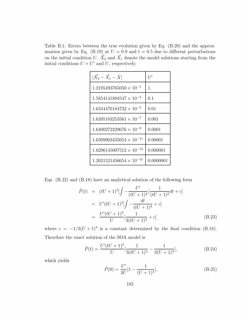
Table B.1: Errors between the true evolution given by Eq. (B.20) and the approx-imation given by Eq. (B.19) at U = 0.9 and t = 0.5 due to different perturbations
on the initial condition U . ~X2 and ~X1 denote the model solutions starting from theinitial conditions U + U ′ and U , respectively.
| ~X2 − ~X1 − X| U ′
1.2195493765050× 10⁻¹ 1.
1.5854141894547× 10⁻³ 0.1
1.6344476184732× 10⁻⁵ 0.01
1.6395183253561× 10⁻⁷ 0.001
1.6400272229676× 10⁻⁹ 0.0001
1.6399903435054× 10⁻¹¹ 0.00001
1.6206145007512× 10⁻¹³ 0.000001
1.2021521456654× 10⁻¹⁵ 0.0000001
Eqs. (B.22) and (B.18) have an analytical solution of the following form
P (t) = (tU + 1)2[∫
− U ′
(tU + 1)2)
1
(tU + 1)2dt+ c]
= U ′(tU + 1)2[∫
− dt
(tU + 1)4+ c]
=U ′(tU + 1)2
U[
1
3(tU + 1)3+ c] (B.23)
where c = −1/3(U + 1)3 is a constant determined by the final condition (B.18).
Therefore the exact solution of the SOA model is
P (t) =U ′(tU + 1)2
U[
1
3(tU + 1)3− 1
3(U + 1)3], (B.24)
which yields
P (0) =U ′
3U[1 − 1
(U + 1)3], (B.25)
185
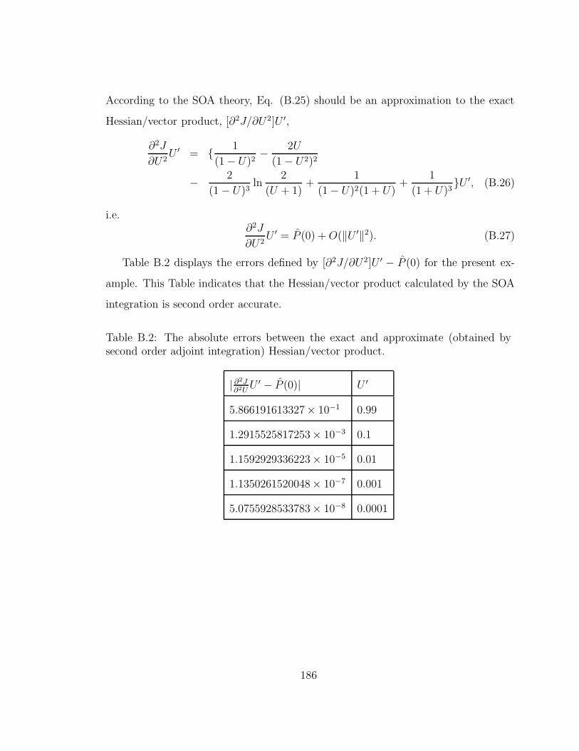
According to the SOA theory, Eq. (B.25) should be an approximation to the exact
Hessian/vector product, [∂2J/∂U2]U ′,
∂2J
∂U2U ′ = { 1
(1 − U)2− 2U
(1 − U2)2
− 2
(1 − U)3ln
2
(U + 1)+
1
(1 − U)2(1 + U)+
1
(1 + U)3}U ′, (B.26)
i.e.∂2J
∂U2U ′ = P (0) +O(‖U ′‖2). (B.27)
Table B.2 displays the errors defined by [∂2J/∂U2]U ′ − P (0) for the present ex-
ample. This Table indicates that the Hessian/vector product calculated by the SOA
integration is second order accurate.
Table B.2: The absolute errors between the exact and approximate (obtained bysecond order adjoint integration) Hessian/vector product.
| ∂2J∂2U
U ′ − P (0)| U ′
5.866191613327× 10⁻¹ 0.99
1.2915525817253× 10⁻³ 0.1
1.1592929336223× 10⁻⁵ 0.01
1.1350261520048× 10⁻⁷ 0.001
5.0755928533783× 10⁻⁸ 0.0001
186
APPENDIX C
TN: NASH’S TRUNCATED NEWTON METHOD.
The Truncated Newton algorithm of Nash [130, 134] is one of the most efficient
large-scale unconstrained minimization algorithms. Schlick and Fogelson [185, 186]
modified the truncated Newton algorithm and developed a FORTRAN package to
solve problems for which some separability and sparsity structure of the Hessian is
available. Here we give a general description of the truncated Newton algorithm of
Nash [130, 134]. The algorithmic form of Nash’s T-N method is:
1. Supply ~X0, an initial approximation to the minimizer ~X and set k=0.
2. Test ~Xk for convergence. Terminate if the following criteria are satisfied:
‖~gk‖ < 10−5 · ‖~g0‖, (C.1)
where ‖~gk‖ is the Euclidean norm of the gradient of the cost function Jk with
respect to the control variables, then stop. Otherwise continue.
3. Solve the Newton equations system
Gk~dk = −~gk, (C.2)
where Gk is an approximation to the Hessian matrix, using a modified-Lanczos
algorithm with preconditioning [134] (also see the additional remarks at the
end of this appendix). If the Hessian matrix is positive definite, the modified-
Lanczos method is equivalent to the linear conjugate-gradient algorithm of
Hestenes and Stiefel [84]. The modified-Lanczos method can be described
briefly as follows:
187
(a) Start the Lanczos process with some vector ~v1, which is chosen as a mul-
tiple of −~g and has ~vT1 ~v1 = 1. Set
~d1 = −~gk. (C.3)
(b) For q = 1, 2, . . ., calculate the matrix-vector product G~vq which is approx-
imated by a finite-differencing scheme along the gradient ~g (we omit the
subscripts k for clarity):
G~vq =~g
(
~X + h~v)
− ~g(
~X)
h, (C.4)
where h is some small positive value such as the cubic root of machine
precision. Note that this formula requires only one additional evaluation
of the gradient in each inner iteration.
(c) Using the Lanczos recurrence relations
βj+1~vj+1 = G~vj − αj~vj − βj~vj−1, j = 1, 2, . . . , q − 1 (C.5)
After q-th step this expression may be written as
GVq = VqTq + βq+1~vj+1~eTq (C.6)
where
Tq =
α1 β2
β2 α2 β3
β3 α3 ·
· · ·
· · ·
· · β
βq αq
(C.7)
188
is a tridiagonal matrix approximating G and αj = ~vTG~vj. The value
βj+1(≤ 0) is chosen so that ‖~vj+1‖2 = 1, ~eq is the q-th column of the q× q
identity matrix.
(d) Calculate the Cholesky factorization factors of Tq, Lq and Dq, where
Tq = LqDqLTq . (C.8)
(e) Determine the (q + 1) -th approximation for the kth iterate of the search
direction by the expression
~dq+1 = ~dq −~rT
q ~vq
Dq
~uq. (C.9)
The value of ~uq is computed from the recurrence relations
~u1 = ~v1, ~uq = ~vq − lq~uq−1, (C.10)
where lq is subdiagonal element (q − 1) of the lower bidiagonal matrix
Lq, Dq is the qth diagonal element and ~rq is the residual of the Newton
equations, ~rq = G~dq + ~g.
(f) If the prescribed truncation criteria
1 − ~g~dq + ~rq~dq
~g~dq+1 + ~rq+1~dq+1
≤ 0.5
q(C.11)
is satisfied, stop the inner iteration; otherwise continue the inner loop
from step b).
4. Set k = k + 1 and update
~Xk+1 = ~Xk + αk~dk, (C.12)
where αk is the step-size obtained by conducting a line search
J( ~Xk + αk~dk) = min
αJ( ~Xk + α~dk), (C.13)
189
using Davidon’s cubic interpolation method for the line search of the step size
and which satisfies the following Wolfe conditions:
f( ~Xk + αk~dk) ≤ f( ~Xk) + β ′αk~g
Tk~dk, (C.14)
and~gk( ~Xk + αk
~dk)T ~dk
~gTk~dk
≤ β, (C.15)
where β ′ = 0.0001, β = 0.9. Go to step 2.
Additional Remarks: In the TN method the Newton equation (C.2) is solved
by performing a limited number of iterations of the linear conjugate-gradient method.
The iterations are terminated (“truncated”) before the system is solved exactly. If
a single linear iteration is used, ~dk will be the steepest-descent direction −~gk; if the
sequence is not truncated, ~dk will be the Newton direction. Thus, the algorithm
computes a vector that interpolates between the steepest-descent direction and the
Newton direction.
The TN method will be successful only when a good direction can be produced
in a rather small number of linear conjugate-gradient iterations, and hence the use
of a good preconditioning is essential. Because the number of iterations required to
solve the Newton’s equation is equal to the number of distinct eigenvalues in exact
arithmetic, the idea of preconditioning transforms the Newton equations to a related
system possessing a more favorable eigenvalue structure. Ideally, the condition num-
ber will be low, and the eigenvalues will cluster near 1. Theoretically, this facilitates
the convergence of the C-G method. Newton’s equations (C.2) are equivalent to the
following equation
(M− 1
2GM− 1
2 )M1
2 ~X = −M− 1
2~g. (C.16)
Let R denote the matrix M− 1
2 GM− 1
2 ; then R has the same eigenvalues as M− 1
2 G,
since M− 1
2 RM− 1
2 = M−1G.
190
The preconditioning matrix M may be chosen in several ways. One source is from
the limited memory quasi-Newton method, where the matrix Hk+1 is an approxima-
tion to the inverse of the Hessian and satisfies the “quasi-Newton condition” for k
pairs of vectors {~pk, ~qk}:
~pj = Hk+1~qj, j = 1, 2, . . . , k. (C.17)
where ~pj = ~Xj+1 − ~Xj, ~qj = ~gj+1 − ~gj. Since G~pj = ~qj,
~pj = Hk+1G~pj, j = 1, 2, . . . , k. (C.18)
and the matrix Hk+1G has k unit eigenvalues with eigenvectors {~pj}. Therefore, this
QN Hk+1 may be used as the preconditioning matrix M−1. In this case, the vector
−Hk+1~gk will be the first nontrivial member of the sequence{
~dq
}
and this search
direction may be used to obtain a better reduction in the function than −~gk. Thus
the search direction will interpolate between the Newton direction and a quasi-Newton
direction.
Since the matrix H is never stored explicitly, Nash [134] uses an approximation
to the diagonal of the Hessian matrix.
191
APPENDIX D
THE CONTINUOUS FORM OF THE ADJOINT EQUATIONS
For the parameter estimation of nudging coefficients, the cost function J can be
defined as an integral
J =1
2
∫ tf
t0
{< W ( ~X − ~Xo), ~X − ~Xo > + < K(G− G), G− G > dt. (D.1)
The dynamical model Eq. (6.11) viewed as strong constraints can be enforced by
introducing a set of undetermined Lagrange multipliers. This leads to the following
Lagrange function
L( ~X,G, P ) = J +∫ tf
t0
< P,−∂~X
∂t+ F ( ~X) +G( ~Xo − ~X) > dt, (D.2)
where P is a vector of Lagrange multiplies to be determined.
The constrained optimization problem is then replaced by a series of unconstrained
minimization problems with respect to the variables U and G. By doing so, the
problem of minimizing the cost function, subject to the model equations, becomes a
problem of finding the stationary points of the Lagrange function. This in turn is
equivalent to the determination of U and G subject to the condition that the gradient
of the Lagrange function vanishes. This leads to the following first-order condition:
∂L
∂X= 0, (D.3)
∂L
∂P= 0, (D.4)
∂L
∂G= 0, (D.5)
192
The solution of Eqs. (D.3-D.5) is called the stationary point of L. Eq. (D.5) results
in
∇GJ +∫ tf
t0
< ( ~Xo − ~X), P > dt = 0, (D.6)
which yields the gradient of the cost function with respect to G
∇GJ = −∫ tf
t0
< ( ~Xo − ~X), P > dt. (D.7)
Eq. (D.4) recovers the original model Eq. (6.11), while (D.3) yields the adjoint
equations
∂J
∂X− ∂
∂X
∫ tf
t0
< P,∂ ~X
∂t− F ( ~X) −G( ~Xo − ~X) > dt = 0, (D.8)
Substituting (D.1) into (D.8) and using integration by parts one obtains
∫ tf
t0
W ( ~X − ~Xo)dt − ∂
∂X{P (tf) ~X(tf) − P (t0) ~X(t0) −
∫ tf
t0
< ~X,∂P
∂t>}
+∫ tf
t0
<∂F
∂ ~X−G,P > dt = 0. (D.9)
If we notice that
∂
∂X{P (tf) ~X(tf) − P (t0) ~X(t0)} = 0, (D.10)
Eq. (D.9) becomes
∫ tf
t0
{∂P∂t
+( ∂F
∂ ~X
)∗P −G∗P +W ( ~X − ~Xo)}dt = 0, (D.11)
for any length of assimilation window tf − t0. Thus the integrand should be zero,
which results in the first order adjoint equation, given by the following equations
−∂P∂t
=(∂F
∂ ~X
)∗P −G∗P +W ( ~X − ~Xo), (D.12)
P (tf) = 0, (D.13)
where P is the adjoint variable in the first order adjoint model and is identical to the
vector of Lagrange multipliers.
193
APPENDIX E
KALMAN FILTERING, VARIATIONAL DATA ASSIMILATION AND
VARIATIONAL NUDGING DATA ASSIMILATION
In this section we give a brief description of the Kalman filtering [68] and the
connection among the KF, nudging, VNDA and VDA.
Starting from the forecast model Eqs. (1.4) and (1.5) which are advanced in
discrete time step ∆t, ~Xn = ~X(tn), tn = n∆t, i.e.
~Xfn = Mn−1
~Xan−1, (E.1)
where the superscript f denotes the forecast and the superscript a stands for analysis,
and M is the discretized form of the system matrix, describing the model dynamics.
A linear unbiased data assimilation scheme for the analysed model state can be
written as
~Xan = ~Xf
n +Gn( ~Xon −Hn
~Xfn−1), (E.2)
where H represents the fact that only certain variables or combinations are observed
as a set of points smaller than the total number of model grid points. The weight
matrix Gn is often called the gain matrix, and the KF approach uses an optimal Gn
to carry out such a linear unbiased data assimilation. The optimality is defined in
the context of the following assumptions.
First assume the true evolution of the atmosphere, ~X tn, is governed by
~X tn = Mn−1
~X tn−1 + btn−1, (E.3)
where btn−1 is a Gaussian white-noise sequence, i.e.
Ebtn = 0, Ebtn(btl)∗ = Qnδnl, (E.4)
194
with E being the expectation operator and δnl being the Kronecker delta function.
The second assumption used in optimizing the weight matrix Gn concerns the error
model for the observations
~Xon = Hn
~X tn + bon, (E.5)
where bon, the observational noise, satisfies
Ebon = 0, Ebon(bol )∗ = Rnδnl. (E.6)
The third assumption is that system noise and observational noise are uncorrelated
to each other:
Ebtn(bon)∗ = 0. (E.7)
Using Eqs. (E.1)-(E.7), one can derive the time evolution of the error covariance
matrix
W an ≡ E( ~Xa
n − ~X tk)
∗( ~Xan − ~X t
k)
= (I −GnHn)W fn (I −GnHn)
∗ +GnRnG∗n, (E.8)
where
W fn ≡ E( ~Xf
n − ~X tk)
∗( ~Xfn − ~X t
k) = Mk−1Wan−1M
∗k−1 +Qk−1. (E.9)
Hence, by advancing W fn and W a
n along with ~Xfn and ~Xa
n, one can know how well the
true state ~X tn is estimated by ~Xa
n for any weight matrix Gn. This in turn permits one
to determine the optimal Gn by minimizing
JKF (Gn) = tr(W an ), (E.10)
where tr denotes the trace of the matrix.
The optimal weight matrix Gn at the n-th time step is obtained by using Eq.
(E.8) for the matrix W an and setting the derivative of JKF (Gn) with respect to each
element of Gn equal to zero. The minimum is obtained at
G∗n ≡ W f
nH∗n(HnW
fnH
∗n +Rn)∗. (E.11)
195
The above linear unbiased data assimilation scheme given by Eqs. (E.1) and (E.2)
with optimal gain matrix G∗n is called the KF [90].
There are two problems which arise in the KF. The first is the computational
complexity of advancing in time the error covariance matrices. While Eqs. (E.1) and
(E.2) represent O(N) computations per time step, Eqs. (E.8) and (E.9) represent,
at face value, O(N 2) computations where N is the dimension of the control variable.
Second, the noise covariance matrices Qn and Rn are assumed to be known in the
subsequent derivation of the optimal Gn. This is not so in practice, and finding the
actual magnitude of system and observational errors is an important function of the
data assimilation process.
The nudging scheme is carried out in the following procedure
~Xan = Mn−1
~Xan−1 +Gn( ~Xo
n −Hn~Xa
n). (E.12)
The optimal nudging coefficients Gn are obtained by minimizing a cost function mea-
suring the distance between the analysis and the observations.
J(U) =1
2
M∑
n=0
< W (C ~Xan − ~Xo
n), (C ~Xan − ~Xo
n) >, (E.13)
From Eqs. (E.1) and (E.10) we see that the core of the KF is the optimal merging
of observation and forecast information in the sense that the expected mean-square
estimation error is minimized at every time step. The VNDA, on the other hand, is
the optimal merging of observations and analysis in the sense that the total differences
between them in a certain window of assimilation is minimized (see Eqs. (1.3) and
(E.12)). The main differences between the KF and the VNDA are:
1. observation errors at different times are assumed to be uncorrelated;
2. the weight matrix Gn at each time step is determined sequentially in the KF,
while the nudging coefficients at each time step in the window of assimilation
196
are obtained simultaneously. However, the two problems of the KF described
above disappear in the VNDA. The computational cost is reduced by using an
adjoint model integration in the parameter-estimation mode of VDA. Moreover,
the VDNA does not require any knowledge of the noise covariance matrices.
Therefore, the estimate NDA, the VNDA and the KF differ from each other mainly
in the choice of the weight matrix Gn. The VDA, on the other hand, takes both the
model forecasts and the observations as perfect, i.e. bfn = 0 and non = 0 when n 6= 0.
It attempts to obtain an optimal initial condition which minimizes the cost function
J(U) =1
2
M∑
n=0
< W (C ~Xfn − ~Xo
n), (C ~Xfn − ~Xo
n) >, (E.14)
The theoretical framework of estimation and control theory provides the founda-
tion of data assimilation techniques. The estimated NDA and the KF are closer to
the estimation theory, the VDA to the optimal control aspect, while the VNDA is a
combination of both [119].
In the nonlinear case, an extended Kalman filter (EKF) [163, 66] can be used.
The EKF differs from the KF in that is uses a nonlinear model to make a forecast
~Xfn = Nn−1
~Xfn−1, (E.15)
where N represents the discretized form of the nonlinear system matrix; and the
forecast error covariances are integrated with the tangent linear model, i.e. Eq. (E.9)
is replaced by
W fn ≡ E( ~Xf
n − ~X tk)
∗( ~Xfn − ~X t
k) = Ak−1Wan−1A
∗k−1 +Qk−1. (E.16)
where A is the Jacobian matrix ∂N/∂ ~X . The EKF brings new features concerning the
time evolution of the forecast error covariances since the nonlinear model is linearized
around a time and space dependent flow configuration to yield the tangent linear
model.
197
For the sake of completeness, the entire extended KF algorithm is included here.
It reads as follows:
~Xfn = An−1
~Xan−1, (E.17)
W fn ≡ E( ~Xf
n − ~X tk)
∗( ~Xfn − ~X t
k) = Ak−1Wan−1A
∗k−1 +Qk−1. (E.18)
G∗n ≡ W f
nH∗n(HnW
fnH
∗n +Rn)∗. (E.19)
W an = (I −G∗
nHn)Wfn , (E.20)
~Xan = ~Xf
n +Gn( ~Xon −Hn
~Xfn−1). (E.21)
where Eq. (E.20) is obtained from Eq. (E.8) under the assumption Gn = G∗n.
198
APPENDIX F
PHYSICAL PROCESSES
The FSUGSM contains parameterizations of a variety of physical effects; these
attempt to simulate diabatic heating, water vapor sources and frictional forces. Di-
abatic heating, due to long wave and short wave radiation, deep cumulus and dry
convection, large scale condensation and sensible heat flux from the (land and sea)
surface are all incorporated into this model. The model contains water vapor sources,
due to deep cumulus convection, large scale condensation and (land and sea) surface
flux. Frictional forces are included through calculations of the surface stress and a
vertical diffusion of momentum and water vapor are also included in the FSUGSM,
although not entirely for physical reasons.
F.0.1 Radiative processes
Forcing due to long wave and short wave radiation has been found to be important
for tropical NWP [126]. The method used for the calculation of the radiative processes
in the FSUGSM is essentially the same as that of Chang [25]. It was originally
implemented in a limited area, multi-level grid point primitive equation model at
FSU. The highlights of this scheme are a specification of the diurnal change (in the
incoming short wave radiation) and a parameterizations of the effects of clouds (on
both the long wave and short wave radiation).
Diurnal change in the incoming solar radiation So (the solar constant: here we
use a value of 1393 Wm−2) is effected by computing the zenith angle (Z) of the sun
199
as a function of local time of day (as well as its latitudinal and seasonal dependent).
The total insolation, So cosZ, is assumed to consist of two components, one which
is scattered by the earth’s atmosphere and another which is absorbed by it. The
scattered and absorbed amounts are assigned to be 65.1% and 34.9% of the total,
respectively. For the absorbed part of the short wave radiation (i.e., that part which
is capable of being absorbed) an absorptivity function, dependent on water vapor
content, temperature, pressure and zenith angle, is defined. This function determined
the amount of depletion the solar radiation undergoes before reaching a given reference
level. Both direct and reflected solar radiation are considered in the model’s radiation
package. The albedo of the earth’s surface for summer season was tabulated from the
works of Posey and Clapp [166] and Kondratyev [94] and interpolated to the Gaussian
grid.
The presence (or lack) of single or multiple layers of clouds is empirically deter-
mined for the radiative computations. Three basic cloud types are permitted: low
(centered at 850 mb), middle (centered at 700 mb) and high (centered at 500 mb).
Clouds are specified from the relative humidity distribution, with minimum threshold
values of 66%, 35% and 26%, respectively, for the presence of the above 3 cloud types.
The fractional coverage of each of the types is then deduced from linear empirical func-
tions of the relative humidity. The presence of clouds increases the absorptivity and
causes partial reflection of the short wave radiation (the cloud albedos are empirically
specified).
The scattered part of the total insolation is assumed to be unimportant in the
atmospheric heating. However, in the heat balance of the earth’s surface, to be
discussed below, the scattered component is included in the total short wave radiation
reaching the ground. Thus, the scattered short wave radiation does play a role in
determining the ground temperature.
200
To compute the net long wave radiation (emitted by the earth’s surface and the
atmosphere) which reaches some reference level, the emissivity method is utilized.
The emissivity of a given atmospheric layer is a function of optical depth (which in
turn is taken to be a function of water vapor content, temperature and pressure). The
long wave radiation emitted from the earth’s surface is determined from the computed
(or, in the case of oceanic points, specified) surface (ground or water) temperature.
The net infrared radiation reaching some reference level is obtained from the emission
of the atmospheric layers above and below that level, plus the terrestrial radiation
(modified by the emissivity between the reference level and the surface).
Clouds are treated as black bodies for long wave radiation calculations. Thus,
clouds modulate the long wave radiation in the model’s atmosphere by producing
enhanced long wave irradiance above and below the cloud layers. If a model level
lies within a cloud, then the long wave irradiance at that level is set to zero. Future
details on long wave (as well as short wave) radiation scheme are found in Chang [25].
The diabatic heating due to short wave and long wave radiation is determined
from the convergence of the flux of radiant energy. Hence, the total (long wave plus
short wave) radiative heating is given by
[∂T
∂t]rad =
−gCpps
(∂FS
∂σ+∂FL
∂σ), (F.1)
where FS and FL are the net short wave and long wave irradiances, respectively.
Equation (F.1) is applied at the σ-levels of the FSUGSM; thus, the net irradiances
are computed at the σ-levels. Finite differences in the vertical then yield the diabatic
heating at the σ-levels.
F.0.2 Cumulus convection and large scale condensation
The diabatic heating caused by deep cumulus convection is recognized as a major
energy source in the tropics. Deep convection also acts as a prominent sink of the
201
moisture in the large scale water vapor budget. Therefore, it is essential to include the
effects of cumulus convection in a global prediction model, even if only in a parametric
sense. An implicit treatment of the life cycles of the individual cumulus clouds and
their interaction with the large scale fields is not practical for models such as the
FSUGSM due to limitations of horizontal resolution. There are a number of existing
schemes for the parameterization of cumulus convection in large scale prognostic
models. The schemes which are most widely used are those of Arakawa and Schubert
[6] and Kuo [101]. At FSU, a slightly modified version of Kuo’s [101] parameterization
method has been used in grid point, tropical prediction models with a fair degree of
success ([92, 96]). The tractability of Kuo’s method also makes it appealing for use
in NWP. This method has therefore been adapted for the FSUGSM.
In the current model, the basic variables which are required for cumulus parame-
terizations are temperature, specific humidity and vertical motion (σ, from which we
can evaluate the vertical p-velocity, ω). These variables are available on the Gaussian
grid points (at the σ-levels) at every time step. The large scale moisture supply, I,
available for convective heating (or, equivalently, rainfall) is defined by
I = −1
g
∫ pcb
pt
ω∂
∂pdp, (F.2)
where pt is the cloud top pressure (i.e., the pressure at which the moist adiabat,
originating from pcb, intersects the model sounding) and pcb is the pressure of the cloud
base. The cloud base is defined by the first model level (proceeding upward from the
bottom) where the relative humidity equals or exceeds 70%. At any time step (for
each Gaussian grid point), parameterized cumulus convection will be invoked if all of
the following conditions are met: (a) the moisture supply, I, is positive; (b) the cloud
base relative humidity criterion is satisfied; and (c) the atmosphere is conditionally
unstable. Conditional instability exits if
∂θ
∂p+θ
T
L(Td)
Cp
∂rS
∂p≥ 0, (F.3)
202
where θ is the potential temperature (although the same notation is used for latitude
and potential temperature, there is no confusion if read consistently) and rS is the
saturation specific humidity.
Following Kuo [102], Kanamitsu [92] and Krishnamurti et al. [96] if the above
condition are satisfied, the convective heating rate is given by
∂T
∂t|conv = aT {
TS − T
∆τ+T
θω∂θ
∂p}, (F.4)
and the convective moistening rate is
∂r
∂t|conv = ar{
rS − r
∆τ}. (F.5)
In (F.4) and (F.5), TS and rS correspond to the saturation values of T and r (water-
vapor mixing ratio), respectively, on the moist adiabat, which passes through pcb, and
∆τ is the cloud time scale (here, following earlier studies using Kuo’s parameterization
scheme with a grid-point model, ∆τ is set to 1800 seconds). The coefficients aT and
ar are determined by means of the following relations:
aT =(1 − b)I
Cp
L(Td)g
∫ pcb
pt{TS−T
∆τ+ T
θω ∂θ
∂p}dp
, (F.6)
ar =bI
1g
∫ pcb
pt{ rS−r
∆τ}dp, (F.7)
where the parameter b specifies the partitioning of the total moisture supply (I) into
heating and moisture. The determination of b has been a subject of great interest
to those scientists working with Kuo’s method of convective parameterization. Kuo
[102] presented observational evidence which suggests that b should be quite close to
zero. Kanamitsu [92] proposed an ad hoc specification of b for use in a prognostic
model. Anthes [5] gave a formula for b which is based on the large scale relative
humidity distribution (in the vertical). However, none of the above formulations were
entirely satisfactory from a physical point of view.
203
Krishnamurti et al. [97] utilized Kuo’s method with the GATE phase III data
(Sept. 1 through 18, 1974 over the eastern tropical Atlantic) to compute convective
rainfall rates. In that study, the available moisture supply (I) was defined as in (F.2)
and Kuo’s [102] scheme was employed in a semi-prognostic manner (i.e., a series
of single time step predictions). It was found that a very close agreement between
observed and computed rainfall rates could be obtained by setting b to be a constant
value of zero. In view of this and the inadequate physical justification for other types
of closure, it was decided to set b to zero for present study. It should be noted that this
implies that the convective moisture is zero in this case (by virtue of (F.5) and (F.7)).
In other words, all of the large scale moisture supply defined by I is condensed out as
rainfall. However, horizontal advection and diffusion of moisture (discussed below)
can still contribute to moistening when the convective parameterization is invoked.
Large scale condensation heating (and rainfall) is simulated in the present model
by the removal of supersaturation whenever it is observed in the prediction. This
phenomenon typically occurs in regions of large scale ascent of air having absolutely
stable (with respect to moist adiabatic) lapse rates, although other processes (such as
radiative cooling) can also cause supersaturation. The numerical procedure for calcu-
lation of the supersaturation heating in the FSUGSM is the same as that described
by Daley et al. [40]. At each time step, the model soundings of temperature and
moisture are adjusted (if supersaturation is found) before any of the other physical
forcing effects are evaluated. Any excess oversaturation is assumed to be condensed
out as rain.
F.0.3 Boundary layer processes
A fairly simply treatment of the planetary boundary layer is used for the FSUGSM.
Over the oceanic Gaussian grid points, the surface fluxes of sensible heat and water va-
por and the surface stresses are calculated from bulk aerodynamics principles. Hence,
204
the sensible heat flux is given by
Fsen = 1.6 × 10⁻³Cpρa(To − Ta)|~Va|, (F.8)
while the water vapor flux is specified by
Fvap = 1.4 × 10⁻³ρa(rSTo − ra)|~Va|, (F.9)
and the surface stress is determined by
Fmom = |~τ | = 1.1 × 10⁻³ρa|~Va|2, (F.10)
where To is monthly climatological sea surface temperature (in this study, for June)
taken from the work of Alexander and Mobley [1] while ρa, Ta, ~Va and ra are the
surface (anemometer level) air density, temperature, wind and specific humidity, re-
spectively. These quantities are obtained by extrapolation from the lowest model
level, assuming a well mixed surface layer (in terms of potential temperature, wind
and relative humidity). The numerical values of the surface exchange coefficients in-
dicated in (F.8) through (F.10) are those suggested by Businger and Seguin [18] from
GATE data.
Over land, the surface fluxes of sensible and latent heat are computed in con-
junction with a determination of heat balance of the earth’s surface. Daytime and
nighttime are treated as separate cases in this formulation. If the net radiation (i.e.,
short wave plus long wave radiation) at the surface is negative (i.e. upward), then
nighttime conditions are presumed. In this case, an empirically determined fraction
of net radiation is used to lower the ground temperature. The remaining radiative
deficit is assumed to be a downward flux of sensible heat which cools the surface
air. The flux of latent heat is set to zero over land areas at night. The calculation
of nighttime surface stress essentially follows the stable surface layer formulation of
Businger et al. [17], which makes use of similarity theory.
205
For the daytime situation, the sensible and latent heat fluxes and the ground
temperature are determined via the iterative solution of an explicit heat balance
equation for the earth’s surface, with the storage term neglected:
0 = Rnet − σBT4o − Fsen − L(Td)Fvap, (F.11)
where Rnet is the net surface radiance (excluding the upward long wave irradiance)
and σB is the Stefan-Boltzmann constant. The fluxes of sensible and latent heat, Fsen
and L(Td)Fvap, are given by relations similar to (F.8) and (F.9). However, rather
than using the saturation specific humidity rS at the ground temperature To in the
calculation of Fvap, a ground wetness (saturation ratio) is used to modify rS. This
ground wetness, gW , is an empirical function of αS, the surface albedo,
gW = 0.85[1 − e−200(0.25−αS)2 ]. (F.12)
For a low albedo (less than 10%) the ground wetness approaches 0.85. For
albedo values greater than 25%, gW is set to zero. This formulation has been ex-
tensively tested and was found to avoid excessively high water vapor fluxes over
tropical land areas. Eq. (F.11) is solved iteratively for the ground temperature To by
Newton-Raphson technique. The daytime surface stress calculation essentially follows
Businger et al. [17].
Above the surface level (over both land and ocean), the fluxes of heat, moisture
and momentum are specified by the mixing length theory, as in Smagorinsky et al.
[191]. That is, the fluxes of sensible heat, water vapor and momentum are respectively
given by
Fsen = −ρ`2m|∂~V
∂z|∂θ∂z, (F.13)
Fvap = −ρ`2m|∂~V
∂z|∂r∂z, (F.14)
Fmom = −ρ`2m|∂~V
∂z||∂
~V
∂z|, (F.15)
206
where `2m is the mixing length, which is a linear function of height. Above 3 km (from
the surface topography), `2m vanishes and the fluxes are therefore zero. However, in
the moisture prediction an additional flux, over that implied by (F.14), is used. This
added flux is defined by an explicit vertical diffusion of water vapor. It is expressed
by∂r
∂t|diff = Kr(σ)
∂2r
∂σ2, (F.16)
where the diffusion coefficient Kr(σ) is given by
Kr(σ) = (5σ − 1.25) × 10−7s−1, (F.17)
Above the σ = 0.25 level, Kr(σ) is set to zero. Thus, the diffusion of moisture is
stronger near the surface level. As noted earlier, in the discussion of the convec-
tive parameterization, all of the large (model) scale vertical advection of moisture is
consumed for the convective rainfall. Here the inclusion of the vertical diffusion of
moisture in vertical column, prevents excessive drying due to the cumulus convection.
F.0.4 Dry convective adjustment
Whenever the lapse rate of potential temperature is found to be dry unstable
(superadiabatic) over a model grid point, a dry convective adjustment is carried out.
This situation typically occurs at the lower levels, over land areas possessing relatively
high ground temperatures (i.e., deserts). The adjustment procedure removes heat to
the top of the layer, while conserving dry static energy (gz+CpT ). The end result of
dry convective adjustment is a dry adiabatic lapse rate in the layer. In practice, this
is done iteratively, checking the model’s atmospheric column from top to bottom for
the occurrence of superadiabatic layers. This is because the adjustment of a given
layer may produce dry instability in the layer below.
207
F.0.5 Surface topography
Since the FSUGSM is a σ-coordinate model in the vertical direction, it allows
for the realistic inclusion of the surface topography (since the earth’s surface is a
coordinate surface). The effects of orography in the prognostic equations appear
mainly through the horizontal variations of q (i.e., ln ps, which is strongly dependent
upon topography). ΦS (the earth’s topography) is spectrally truncated as the other
variables in the model.
F.0.6 Computational requirements
The implementation of the transform technique in the FSUGSM requires that
(in the computer code) memory storage be allocated to both grid-point and spectral
coefficient representations of the dependent variables. All the spectral coefficients
reside in the core simultaneously; however, only one latitude of the grid-point values
(for all model levels) is stored at any instant. Contributions from each latitude to
the spectral transforms are accumulated successively in the computer program, thus
negating the need to store the entire grid in memory. Physical effects computations
make use of column models, and therefore only require storage for the vertical levels.
208
REFERENCES
[1] Alexander, R. C. and Mobley, 1974: Monthly average sea surface temperaturesand ice-pack limits on a 1◦ global grid. Rand Corporation Report, Santa Monica,CA, 90406, 30 pp.
[2] Andersson, E., A. Hollingsworth, G. Kelly, P. Lonnberg, J. Pailleux, and Z.Zhang, 1991: Global observing system experiments on operational statisticalretrievals of satellite sounding data. Mon. Wea. Rev., 199, 1851-1864.
[3] Andersson, E., J. Pailleux, J. N. Thepaut, J. R. Eyre, A. P. McNally, G. A. Kellyand P. Courtier, 1992: Use of radiance in 3D/4D variational data assimilation.In Proc. of ECMWF Workshop on variational assimilation with emphasis onthree-dimensional aspects, Shinfield Park, Reading RG2 9AX, UK, 123-156.
[4] Anthes, R. A., 1974: Data assimilation and initialization of hurricane predictionmodels. J. Atmos. Sci., 31, 702-719.
[5] Anthes, R. A., 1977: A cumulus parameterization scheme utilizing an one di-mensional cloud model. Mon. Wea. Rev., 105, 270-286.
[6] Arakawa, A. and Schubert W. H., 1974: Interaction of a cumulus cloud ensemblewith the large scale environment, Part I. J. Atmos. Sci., 31, 674-701.
[7] Asselin, R., 1972: Frequency filter for time integrations. Mon. Wea. Rev., 100,487-490.
[8] Banks, H. T. and K. Kunisch, 1989: Estimation techniques for distributed pa-rameter systems. Birkhauser, Boston (Systems & Control: Formulations & Ap-plications), Vol. 11, 315 pp.
[9] Bao, J. W. and T. T. Warner, 1993: Treatment of On/Off switches in the adjointmethod: FDDA experiments with a simple model. Tellus, in press.
[10] Bertsekas, D. P. 1982: Constrained optimization and Lagrange multiplier meth-ods. Addison-Wesley, 491 pp.
[11] Bernardet, P., S. Farges and K. Yassine, 1992: Adjoint of non-hydrostatic model.In Proc. of ECMWF Workshop on variational assimilation with emphasis onthree-dimensional aspects, Shinfield Park, Reading RG2 9AX, UK, 339-374.
209
[12] Bourke, W. 1972: An efficient one level primitive equation spectral model. Mon.Wea. Rev., 100, 683-689.
[13] Bourke, W. 1974: A multi-level spectral model. I –Formulation and hemisphereintegrations. Mon. Wea. Rev., 102, 687-710.
[14] Buckley, A. G. and A. Lenir, 1983: QN-like variable storage conjugate gradients.Math. Prog., 27, 155-175.
[15] Burger, J., J. L. Brizaut and M. Pogu, 1992: Comparison of two methods for thecalculation of the gradient and of the Hessian of the cost functions associatedwith differential systems. Mathematics and Computers in Simulation, 34, 551-562.
[16] Bus, J. C. P., 1977: Convergence of Newton-like methods for solving systems ofnonlinear equations. Numerische Mathematik, 27, 271-281.
[17] Businger, J. A.,J. C. Wyngaard, Y. Izumi and E. F. Bradley, 1971: Flux-profilerelationship in the atmospheric surface layer. J. Atmos. Sci., 28, 181-189.
[18] Businger, J. A. and W. Seguin, 1977: Transport across the air-sea interface:air-sea surface fluxes of latent and sensible heat and momentum. In Proc. of theGATE Workshop, published by the National Center for Atmospheric Research,Boulder, Colorado, 80303, 441-453.
[19] Cacuci, Dan G., 1981: Sensitivity theory for nonlinear systems. I: Nonlinearfunctional analysis approach. J. Math. Phy. 22 (12),2794-2803.
[20] Cacuci, Dan G., 1981: Sensitivity theory for nonlinear systems. II. Extensionsto additional classes of responses. J. Math. Phy. 22 (12), 2803-2812.
[21] Cai, Y. and I. M. Navon, 1993: Iterative domain decomposition algorithms:Theory and application. High performance computing in the geoscience, editedby F.X. Le Dimet, Klumer Academic Publishers B.V. 000-000.
[22] Carrera, J. and P. S. Neuman, 1986: estimation of aquifer parameters undertransient and steady state conditions, 1: Maximum likelihood method methodincorporating prior information. Water Resources Research, 22 (2), 199-210.
[23] Carrera, J. and P. S. Neuman, 1986: estimation of aquifer parameters undertransient and steady state conditions, 2: Uniqueness, stability and solutionalgorithms. Water Resources Research, 22 (2), 211-227.
210
[24] Carrera, J. and P. S. Neuman, 1986: estimation of aquifer parameters undertransient and steady state conditions, 3: Application to synthetic and fielddata. Water Resources Research, 22 (2), 228-242.
[25] Chang, C. B., 1979: On the influences of solar radiation and diurnal varia-tion of surface temperatures on African disturbances. Rept. No. 79-3, Dept. ofMeteorology, Florida State University, Tallahassee, FL 32306, 157 pp.
[26] Chao W. C. and L. Chang, 1991: Development of a 4-dimensional analysissystem using the adjoint method at GLA. part 1: dynamics. Mon. Wea. Rev.,120, 1661-1673.
[27] Charney, J. G., R. FjØrtoft and J. Von Neumann, 1950: Numerical integrationof the barotropic vorticity equation. Tellus, 2, 237-257.
[28] Charney, J. G., M. Halem and R. Jastrow, 1969: Use of incomplete historicaldata to infer the present state of the atmosphere. J. Atmos. Sci., 2, 1160-1163.
[29] Cohn, S. E., 1982: Methods of sequential estimation for determining initial datain numerical weather prediction. Ph.D Thesis, New York University, 183 pp.
[30] Cohn, S. E. and D. F. Parrish, 1991: The behavior of forecast error covariancesfor a Kalman filter in two dimensions. Mon. Wea. Rev., 119, 1757-1785.
[31] Cohn, S., 1993: The Kalman filtering versus variational analysis debate. Per-sonal communication.
[32] Cohn, S, 1993: Dynamics of short-term univariate forecast error covariances.Mon. Wea. Rev., 121 (11), 3123-3149.
[33] Courtier, P.,1985: Experiments in data assimilation using the adjoint modeltechnique. Workshop on High-Resolution Analysis ECMWF (UK) June 1985.
[34] Courtier, P. and O.Talagrand, 1987: Variational assimilation of meteorologi-cal observations with the adjoint equations Part 2. Numerical results.Q. J. R.Meteorol. Soc., 113, 1329-1347.
[35] Courtier, P., 1987: Application du controle optimal a la prevision numerique enmeteorologie. These de Doctorat de l’Universite-Pierre-et-Marie, Paris.
[36] Courtier, P. and O.Talagrand, 1990: Variational assimilation of meteorologicalobservations with direct and adjoint shallow-water equations. Tellus., 42A, 531-549.
211
[37] Courtier, P. and J. N. Thepaut, 1992: A strategy for operational implementationof 4D-VAR. In Proc. of ECMWF Workshop on variational assimilation, withspecial emphasis on three-dimensional aspects, Shinfield Park, Reading RG29AX, UK, 437-463.
[38] Courtier, P., P. Unden, W. Heckley, D. Vasijevic, E. Andersson, J. N. Thepaut,F. Rabier and R. Hoffman, 1993: Progress in variational data assimilation atECMWF. Research activities in atmospheric and oceanic modeling, G. J. Boer(ed.), Report No., 18, 1.42.
[39] Cressman, G., 1959: An operational objective analysis system. Mon. Wea. Rev.,87, 367-374.
[40] Daley, R., Girard C., Henderson and J. Simmonds, 1976: Short-term forecastingwith a multi-level spectral primitive equation model. Part I – Model Formula-tion. Atmosphere, 14 (12), 98-116.
[41] Daley, R., 1991: Atmospheric data analysis. Cambridge University Press, Cam-bridge.
[42] Daley, R, 1993: Estimating observation error statistics for atmospheric dataassimilation. Ann. Geophysicae, 11, 634-647.
[43] Daley. R, and R. Menard, 1993: Spectral characteristics of Kalman filter systemsfor atmospheric data assimilation. Mon. Wea. Rev, 121, (5), 1554-1565.
[44] Daley. R, and R. Menard, 1993: Evaluation of assimilation systems. Notes forthree lectures at the international summer school on assimilation of meteorolog-ical and oceanographic observations. La Garde, France, August 2-27.
[45] Das, S. K. and R. W. Lardner, 1992: Variational parameter estimation for atwo-demensional numerical tidal model. International Journal for NumericalMethods in Fluids, 15, 313-327.
[46] Davidon, W. C., 1959: Variable metric method for minimization. A. E. C. Re-search and Development Report, ANL-5990 (Rev.).
[47] Davis H. E. and R. E. Turner, 1977: Updating prediction models by dynamicrelaxation. An examination of the technique. Q. J. R. Meteorol. Soc., 103, 225-245
[48] Dembo, R. S., S. C. Eisenstat and T. Steihaug, 1982: Inexact Newton methods.SIAM Journal of Numerical analysis, 19, 400-408.
212
[49] Dembo, R. S. and T. Steihaug, 1983: Truncated-Newton algorithms for large-scale unconstrained optimization. Math. Prog., 26, 190-212.
[50] Derber, J. C.,1985: The variational four dimensional assimilation of analysisusing filtered models as constraints. Ph.D. Thesis, Univ. of Wisconsin-Madison,141 pp.
[51] Derber, J. C.,1987: Variational four dimensional analysis using the quasi-geostrophic constraint. Mon. Wea. Rev., 115, 998-1008.
[52] Derber, J. C., 1989: A variational continuous assimilation technique. Mon. Wea.Rev., 117, 2437-2446.
[53] Derber, J. C., D. F. Parrish and S. J. Lord, 1991: The new global operationalanalysis system at the National Meteorological Center. Weather and Forecast,6, 538-547.
[54] Derber, John C., David F. Parrish and Joseph G. Sela, 1992: The SSI analysissystem and extensions to 4-D. In Proc. of ECMWF Workshop on variational as-similation with emphasis on three-dimensional aspects, Shinfield Park, ReadingRG2 9AX, UK, 15-29.
[55] Dixon, L. C. W., 1991: Use of automatic differentiation for calculating Hessiansand Newton steps. Automatic differentiation of algorithms: theory, implemen-tation, and application. Andreas Griewank and George F. Corliss (eds.), SIAM,Philadelphia, 115-125.
[56] Ehrendorfer, M., 1992: Four-dimensional data assimilation: comparison of vari-ational and sequential algorithms. Q. J. R. Meteorol. Soc., 118, 673-713.
[57] Eliassen, A., 1954: Provisional report on calculation of spatial covariance andautocorrelation of the pressure field. Report #5, Institute of Weather and Cli-mate Res., Academy of Science, Oslo, 11 pp.
[58] Errico, R. M., Tomislava Vukicevic, and Kevin Raeder, 1993: Examination ofthe accuracy of a tangent linear model. Submitted to Tellus.
[59] Eyre, J. R., G. A. Kelly, A. P. McNally and E. Andersson, 1993: Assimilationof TOVS radiance information through one dimensional variational analysis.Research activities in atmospheric and oceanic modeling, G. J. Boer (ed.), ReportNo., 18, 1.43.
[60] Fletcher, R., 1980: Practical method of optimization. Vol. 1: Unconstrainedoptimization. Wiley and Sons, New York, 120 pp.
213
[61] Fletcher, R., 1980: Practical method of optimization. Vol. 2: Constrained opti-mization. Wiley and Sons, New York, 224 pp.
[62] Fletcher, R., 1987: Practical methods of optimization. Volume 1. 2nd ed., JohnWiley, Chichester, New York.
[63] Gandin, L. S., 1963: Objective analysis of meteorological fields. Gidrometeorol.Izd. Leningrad (in Russian), English Translation by Israel Program for ScientificTranslations, Jerusalem, 1965, 242 pp.
[64] Ghil, M., B. Shkoller and V. Yangarber, 1977: A balanced diagnostic systemcompatible with a barotropic prognostic model. Mon. Wea. Rev., 105, 1223-1238.
[65] Ghil, M., S. Cohn, J. Tavantzis, K. Bube, and E. Issacson, 1981: Application ofestimation theory to numerical weather prediction. L. Bengtsson, M. Ghil andE. Kallen (eds.), Dynamic Meteorology: Data assimilation methods, Springer-Verlag, New York, 139-244.
[66] Ghil, M., S. E. Cohn, and A. Dalcher, 1982: Sequential estimation, data assimi-lation, and initialization. D. Williamson (ed.), The interaction between objectiveanalysis and initialization, Publ. Meteorol., 127 (Proc. 14th standard seminar),McGill University, Montreal, 83-97.
[67] Ghil, M., 1986: Sequential estimation and satellite data assimilation in meteo-rology and oceanography. Y. K. Sasaki, T. Gat-Chen, L. White, M. M. Zaman,C. Zieler, L. P. Chang and D. J. Rusk (ed.), Variational Methods in Geosciences,Elsevier, Amsterdam, 91-100.
[68] Ghil, M. and P. Malonotte-Rizzoli, 1991: Data assimilation in meteorology andoceanography. Adv. Geophys., 33, 141-266.
[69] Gilbert, J. C., 1992: Automatic differentiation and iterative processes. Opti-mization Methods and Software, 1, 13-21.
[70] Gill, P. E. and W. Murray, 1972: Quasi-Newton methods for unconstrainedoptimization. J. Inst. Maths Applics, 9, 91-108.
[71] Gill, P. E. and W. Murray, 1974: Numerical methods for unconstrained opti-mization. Academic Press, London and New-York, 283 pp.
[72] Gill, P. E. and W. Murray, 1979: Newton-type methods for unconstrained andlinearly constrained optimization. Math. Prog., 28, 311-350.
214
[73] Gill, P. E. and W. Murray, 1981: Practical optimization. Academic Press, 401pp.
[74] Gill, P. E., W. Murray, M. C. Saunders and M. H. Wright, 1983: Comput-ing forward-difference intervals for numerical optimization. SIAM J. Sci. Stat.Comput., 4, 310-321.
[75] Grammeltvedt, A., 1969: A survey of finite-difference schemes for the primitiveequations for a barotropic fluid. Mon. Wea. Rev., 97, 387-404.
[76] Griewank, A. and Ph. L. Toint, 1982: Partitioned variable metric updates forlarge structured optimization problems. Numer. Math., 39, 119-137.
[77] Griewank, A. and George F. Corliss., 1991: Automatic differentiation of algo-rithms: theory, implementation, and application, SIAM, Philadelphia, 353 pp.
[78] Hall, M. C. G., D. G. Cacuci and M. E. Schlesinger, 1982: Sensitivity analysisof a Radiative-Convective Model by the Adjoint Method. J. of the Atmos. Sci.,39, 2038-2050.
[79] Hall, M. C. G. and D. G. Cacuci, 1983: Physical interpretation of the adjointfunctions for sensitivity analysis of atmospheric models. J. of Atmos. Sci., 40,2537-2546.
[80] Hall, M. C. G., 1986: Application of adjoint sensitivity theory to an atmosphericgeneral circulation model. J. Atmos. Sci., 43, 2644-2657.
[81] Haltiner, G. J. and R. T. Williams, 1980: Numerical prediction and dynamicmeteorology. John Wiley & Sons, New York, 477 pp.
[82] Hamming, R. W., 1973: Numerical methods for scientists and engineers, 2ndedition, McGraw-Hill and New York.
[83] Heckley, W. A., P. Courtier and E. Andersson, 1992: The ECMWF varia-tional analysis: general formulation and use of background information. InProc. of ECMWF Workshop on variational assimilation with emphasis on three-dimensional aspects, Shinfield Park, Reading RG2 9AX, UK, 49-94.
[84] Hestenes M. and E. Stiefel, 1952: Methods of conjugate gradients for solvinglinear systems. J. Res. National Bureau of Standards, 45, 409-436.
[85] Hoffmann, R. N., 1982: SASS wind ambiguity removal by direct minimization.Mon. Wea. Rev., 110, 434-445.
215
[86] Hoffmann, R. N., 1984: SASS wind ambiguity removal by direct minimization.Part II: Use of smoothness and dynamical constraints. Mon. Wea. Rev., 112,1829-1852.
[87] Hoffmann, R. N., 1986: A four dimensional analysis exactly satisfying equationsof motion. Mon. Wea. Rev., 114, 388-397.
[88] Hoke, J. E. and R. A. Anthes, 1976: The initialization of numerical models bya dynamic initialization technique. Mon. Wea. Rev., 104, 1551-1556.
[89] Horton, C. W., L. E. Reichl and V. G. Szebehely, (editors), 1983: Long-timeprediction in dynamics, Wiley-Interscience, New York, 496 pp.
[90] Kalman, R. E., 1960: A new approach to linear filtering and prediction problems.trans. ASME, J. Basic Eng., 82D, 35-45.
[91] Kalman, R. E. and R. S. Bucy, 1961: New results in linear filtering and predic-tion theory. Trans. ASME, J. Basic Eng., 82, 35-45.
[92] Kanamitsu, M., 1975: On numerical prediction over a global tropical belt. Rept.No. 75-1, Dept. of Meteorology, Florida State University, Tallahassee, FL 32306,282 pp.
[93] Kitamura, S. and S.Nakagiri, 1977: Identifiability of spatially varying and con-stant parameters in distributed systems of parabolic type. SIAM, Journal onControl and Optimization, 15, 785-802.
[94] Kondratyev, K. Ya., 1972: Radiation processes in the atmosphere. World Mete-orological Organization Publication No. 309, Geneva, Switzerland, 214 pp.
[95] Kontarev, G., 1980: The adjoint equation technique applied to meteorologicalproblem. ECMWF Tech. Rep., Reading, U. K., 21, 1-21 pp.
[96] Krishnamurti, T. N., Pan H. Chang C. B., Ploshay J. and Oodally W., 1979:Numerical weather prediction for GATE. Quart. J. Roy. Met. Soc., 108, 979-1010.
[97] Krishnamurti, T. N., Ramanathan Y., Pan H. Pasch R. J. and Molinari J., 1980:Cumulus parameterization and rainfall rates I. Mon. Wea. Rev., 108, 465-472.
[98] Krishnamurti, T. N., X. Jishan, H. S. Bedi, K. Ingles and D. Oosterhof, 1991:Physical initialization for numerical weather prediction over tropics, Tellus,43A, 53-81.
216
[99] Krishnamurti, T. N.,H. S. Bedi and K. Ingles, 1993: Physical initialization usingSSM/I rain rates. Tellus, 45A, 247-269.
[100] Krylov, V. I., 1962: Approximate calculation of integrals. ACM MonographSeries, the MacMillan Company, New York, NY.
[101] Kuo, H. L., 1965: On formulation and intensification of tropical cyclonesthrough latent heat release by cumulus convection. J. Atmos. Sci., 22, 40-63.
[102] Kuo, H. L., 1974: Further studies of the parameterization of the influence ofcumulus convection on large-scale flow. J. of Atmos. Sci., 31, 1232-1240.
[103] Lacarra, J. F. and O. Talagrand, 1988: Short-range evolution of small pertur-bations in a barotropic model. Tellus, 40A, 81-95.
[104] Lardner, R. W., A. H. Al-Rabeh and N. Gunay, 1993: optimal estimation ofparameters for a two-dimensional hydrodynamical model of the Arabian Gulf.Personal communication. Water Resource and Environment Division, ResearchInstitute, King Fahd University of Petroleum and Minerals, Dhahran, SaudiArabia.
[105] Lardner, R. W., 1993: Optimal control of open boundary conditions for a nu-merical tidal model. Computer Methods in Applied Mechanics and Engineering,102, 367-387.
[106] Le Dimet, F. X., 1982: A general formalism of variational analysis. CIMMSReport, Norman, OK 73091, 22, 1-34 pp.
[107] Le Dimet, F. X. and A. Nouailler,1986: Assimilation of Dynamics in Geo-sciences. Y. K. Sasaki, Editor, Elsevier, Amsterdam, 181-198.
[108] Le Dimet, F. X. and O. Talagrand, 1986: Variational algorithms for analysisand assimilation of meteorological observations: Theoretical aspects. Tellus,38A, 97-110.
[109] Le Dimet, F. X. and I. M. Navon, 1988: Variational and optimization methodsin meteorology: a review. Tech. Rep. FSU-SCRI-88-144, Florida State Univer-sity, Tallahassee, Florida, 83 pp.
[110] Legler, D. M., I. M. Navon and J. J. O’Brien, 1989: Objective analysis and as-similation of meteorological observations: theoretical aspects. Mon. Wea. Rev.,38A, 97-110.
217
[111] Legler, D. M. and I. M. Navon, 1991: VARIATM–A Fortran code for objec-tive analysis of pseudo-stress with large-scale conjugate-gradient minimization.Computers and Geosciences, 17 (1), 1-21.
[112] Lewis, J. M. and J. C. Derber, 1985: The use of adjoint equations to solve avariational adjustment problem with advective constraints. Tellus, 37A, 309-322.
[113] Li, Yong, I. M. Navon, P. Courtier and P. Gauthier, 1993: Variational dataassimilation with a semi-implicit semi-Lagrangian global shallow-water equationmodel and its adjoint. Mon. Wea. Rev., 121, 159-169.
[114] Li, Y. and K. K. Droegemeier, 1993: The influence of diffusion and associatederrors on the adjoint data assimilation technique. Tellus, 45A, 1-14.
[115] Li, Y., I. M. Navon, W. Y. Yang, X. L. Zou, J. R. Bates, S. Moorthi and R. W.Higgins, 1993: 4-D assimilation experiments with a multilevel semi-Lagrangiansemi-implicit GCM. Mon. Wea. Rev., in press.
[116] Lions J. L., 1971: Optimal control of systems governed by partial differentialequations. Translated by S. K. Mitter, Springer-Verlag, Berlin-Heidelberg, 404pp.
[117] Liu, D. C and Jorge Nocedal, 1989: On the limited memory BFGS method forlarge scale minimization. Math. Prog., 45, 503-528.
[118] Lorenc, A. C., 1981: A global three-dimensional multivariate statistical inter-polation scheme. Mon. Wea. Rev., 109, 701-721.
[119] Lorenc, A. C.,1986: Analysis methods for numerical weather prediction. Q. J.R. Meteorol. Soc., 112, 1177-1194.
[120] Lorenc, A. C., 1988 a: Optimal nonlinear objective analysis. Q. J. R. Meteorol.Soc., 114, 205 -240.
[121] Lorenc, A. C., 1988 b: A practical approximation to optimal four dimensionalobjective analysis. Mon. Wea. Rev., 116, 730-745.
[122] Lorenc, A. C., R. S. Bell and B. Macpherson, 1991: The meteorological officeanalysis correction data assimilation scheme. Q. J. R. Meteorol. Soc., 117, 59-89.
[123] Luenberger, David G.,1984: Linear and nonlinear programming. 2nd edition,Addison-Wesley Inc., Reading, MA, 491 pp.
218
[124] Lyne, W. H., R. Swinbank and N. T. Birch, 1982: A data assimilation experi-ment and the global circulation during the FGGE special observing periods. Q.J. R. Meteorol. Soc., 108, 575-594.
[125] Machenhauer, B., 1977: On the dynamics of gravity oscillations in a shallowwater model, with application to nonlinear normal mode initialization. Beitr.Phys. Atmos., 50, 253-271.
[126] Manabe, S., D. G.Hahn, and Jr. J. L. Holloway, 1974: The seasonal variationof the tropical circulation as simulated by a global model of the atmosphere. J.Atmos. Sci., 31, 43-83.
[127] Marchuk, G. I., 1974: Numerical solution of the problem of dynamics of atmo-sphere and ocean (in Russian). Leningrad, Gidrometeoizdat, 303 pp.
[128] Moore, A. M, and B. F. Farrell, 1993: Rapid perturbation growth on spa-tially and temporally varying oceanic flows determined using adjoint method:application to the gulf stream. J. Phys. Oceanogr., 23, 1682-1702.
[129] Nash, S. G., 1982: Truncated-Newton methods. Ph.D. Thesis, Computer Sci-ence Department, Stanford University, CA.
[130] Nash, S. G., 1984: Newton-type minimization via the Lanczos method. SIAMJ. Numer. Anal., 21 (4), 770-788.
[131] Nash, S. G., 1984: Truncated-Newton methods for large-scale function mini-mization. Applications of Nonlinear Programming to Optimization and Control,H.E. Rauch (ed.), Pergamon Press, Oxford, 91-100.
[132] Nash, S. G., 1984: User’s guide for TN/TNBC: Fortran routines for nonlinearoptimization. Tech. Rep. No., 397, 17 pp.
[133] Nash, S. G., 1984: Solving nonlinear programming problems using truncated-Newton techniques. Numerical optimization, P. T. Boggs, R. H. Byrd and R. B.Schnabel (ed.), SIAM, Philadelphia, 119-136.
[134] Nash, S. G., 1985: Preconditioning of truncated-Newton methods. SIAM J.Sci. Stat. Comput., 6 (3), 599-616.
[135] Nash, S. G. and A. Sofer, 1989: Block truncated-Newton methods for paralleloptimization. Math. Prog., 45, 529-546.
[136] Nash, S. G. and A. Sofer, 1989: A parallel line search for Newton type methodsin computer science and statistics. In Proc. 21-st Symposium on the Interface,K. Berk and L. Malone (ed.), ASA, 134-137.
219
[137] Nash, S. G. and Jorge Nocedal, 1989: A numerical study of the limited memoryBFGS method and the truncated-Newton method for large scale optimization.Tech. Rep. NAM, 02, Dept. of Electrical Engineering and Computer Science,Northwestern University, Dec., 19 pp.
[138] Nash, S. G. and A. Sofer, 1990: Assessing a search direction within a truncated-Newton method. Operations Research Letters, 9 (4), 219-221.
[139] Navon, I. M., 1981: Implementation of ‘a posteriori’ method for enforcing con-servation of potential enstrophy and mass in discretized shallow water equationsmodels. Mon. Wea. Rev., 109, 946-958.
[140] Navon, I. M., 1982: ‘A posteriori’ numerical techniques for enforcing simultane-ous conservation of the integral invariants. Notes on numerical fluid mechanics,Henri Viviand (ed.), GAMM, Vol. 2, 230-241.
[141] Navon, I. M. and R. de Villiers, 1983: Combined penalty multiplier optimiza-tion methods to enforce integral invariants conservation. Mon. Wea. Rev., 111,1228-1243.
[142] Navon, I. M., 1985: A review of variational optimization methods in meteo-rology. Proc. of the International Symposium on Variational Methods in Geo-sciences, Y. K. Sasaki (ed.), University of Oklahoma, Norman, OK 1–5, october15–17.
[143] Navon, I. M., 1986: A review of variational and optimization methods in mete-orology. Festive Volume of the International Symposium on Variational Methodsin Geosciences (Y.K. Sasaki, Ed. ), Elsevier Science Pub. Co. Developments inGeo-mathematics, Vol. 5, 29-34.
[144] Navon, I. M. and D. M. Legler, 1987: Conjugate gradient methods for largescale minimization in meteorology. Mon. Wea. Rev., 115, 1479-1502.
[145] Navon, I. M., 1987: The Bayliss-Isaacson algorithm and the constraint restora-tion method are equivalent. Meteorology and Atmospheric Physics, 13, 143-152.
[146] Navon, I. M., P. K. H. Phua and M. Ramamurthy, 1988: Vectorization ofconjugate-gradient methods for large-scale minimization. In Proceeding Super-computing’88, IEEE computer society and ACM SIGARCH, WASHINGTON,DC, (Reviewed by the IEEE Computer Society Scientific Review Board), 410-419.
[147] Navon, I. M., P. K. H. Phua and M. Ramamurthy, 1990: Vectorization ofconjugate-gradient methods for large-scale minimization. J. O. T. A., 66 (1),71-94.
220
[148] Navon, I. M. and X. Zou, 1991: Application of the adjoint model in meteorol-ogy. In Proceedings of the international conference on automatic differentiationof algorithms: Theory, Implementation and Application, SIAM Publications, A.Griewank and G. Corliss (Eds.), SIAM, Philadelphia, PA.
[149] Navon, I. M., X. L. Zou, J. Derber and J. Sela, 1992: Variational data as-similation with an adiabatic version of the NMC Spectral Model. Mon. Wea.Rev.,122, 1433-1446.
[150] Navon, I. M. and Y. Cai, 1993: Domain decomposition and parallel processingof a finite-element model of the shallow-water equations. Computer Methods inApplied Mechanics and Engineering, 106, No. 1-2, 179-212.
[151] Navon, I. M., 1993: Application of variational methodology in the context ofa diabatic version of NASA/GLA SLSI model. Proposal to NASA, 77 pp.
[152] Navon, I. M., N. J. Zabusky and X. Zou, 1993: Variational data assimilationwith a coarse-resolution shallow water equations model using high-resolutionshallow water equations model. Research activities in atmospheric and oceanicmodeling, G. J. Boer (ed.), Report No., 18, 1.46-1.47.
[153] Neuman, S. P., 1980: A statistical approach to the inverse problem of aquiferhydrology, 3. Improved solution method and added perspective. Water Re-sources Research, 16 (2), 331-346.
[154] Nocedal, J., 1980: Updating quasi-Newton matrices with limited storage.Mathematics of Computation, 35, 773-782.
[155] O’Leary, D. P., 1983: A discrete Newton algorithm for minimizing a functionof many variables. Math. Prog., 23, 20-23.
[156] Orszag, Steven A., 1970: Transform method for calculation of vector coupledsums: application to the spectral form of the vorticity equation. J. Atmos. Sci.,27, 890-895.
[157] Pailleux, J., W. Heckly, D. Vasiljevic, J. N. Thepaut, F. Rabier, C. Cardinaliand E. Andersson, 1991: Development of a variational assimilation system.ECMWF Research Department Technical Memorandum 179, Reading, U.K..
[158] Pailleux, J., 1992: Organisation of 3D variational analysis within the”IFS/ARPEGE” project future plans at meteo France. In Proc. of ECMWFWorkshop on variational assimilation with emphasis on three-dimensional as-pects, Shinfield Park, Reading RG2 9AX, UK, 37-46.
221
[159] Panchang, V. G. and J. J. O’Brien, 1989: On the determination of hydraulicmodel parameters using the strong constraint formulation. in Modeling MarineSystems, I. Ed. A. M. Davies. CRC Press, Inc, 5-18 pp.
[160] Panofsky, H., 1949: Objective weather map analysis. J. Meteorol., 6, 386-392.
[161] Parrish, D. and J. Derber, 1992: The National Meteorological Center’s spectralstatistical interpolation analysis system. Mon. Wea. Rev., 120, 1747-1763.
[162] Pasch, P. J., 1983: On the onset of the planetary scale monsoon. Ph.D. Thesis,Department of Meteorology, FSU, Tallahassee, FL.
[163] Gauthier, P. and P. Courtier, 1992: Data assimilation with an extendedKalman filter. In Proc. of ECMWF Workshop on variational assimilation withemphasis on three-dimensional aspects, Shinfield Park, Reading RG2 9AX, UK,171-190.
[164] Penenko, V. and N. N. Obraztsov, 1976: A variational initialization method forthe fields of the meteorological elements. Meteorol. Gidrol. (English translation),11, 1-11.
[165] Phillips, N. A., 1976: The impact of synoptic observing and analysis systemson flow pattern forecasts. Bull. Am. Meteorol. Soc.,, 57, 1225-1328.
[166] Posey, J. W. and P. F. Clapp, 1964: Global distribution of normal surfacealbedo. Geofisica Internacional (Mexico), 4, 33-48.
[167] Powell, M. J. D., 1982: Nonlinear optimization 1981. Academic Press, London,298 pp.
[168] Rabier, F. P. Courtier and O. Talagrand, 1992: An application of adjointmodels to sensitivity analysis. Beitr. Phys. Atmos., 65 (3), 177-192.
[169] Rabier, F. and P. Courtier, 1992: Four-dimensional assimilation in the presenceof baroclinic instability. Q. J. R. Meteorol. Soc., 118, 649-672.
[170] Rabier, F., P. Courtier, J. Pailleux, O. Talagrand, J. N. Thepaut and D. Vasil-jevic, 1992: Comparison of four-dimensional variational assimilation with sim-plified sequential assimilation. In Proc. of ECMWF Workshop on variationalassimilation with emphasis on three-dimensional aspects, Shinfield Park, Read-ing RG2 9AX, UK, 271-325.
[171] Rabier, F., P. Courtier, J. Pailleux, O. Talagrand, and D. Vasiljevic, 1993:A comparison between four-dimensional variational assimilation and simplifiedsequential assimilation relying on three-dimensional variational analysis. Q. J.R. Meteorol. Soc. 119, 845-880.
222
[172] Ramamurthy, M. K. and F. H. Carr, 1987: Four-dimensional data assimilationin the monsoon region. Part I: Experiments with wind data. Mon. Wea. Rev.,115, 1678-1706.
[173] Ramamurthy, M. K. and I.M. Navon, 1990: Application of a conjugate-gradientmethod to variational assimilation of meteorological fields. International sym-posium on assimilation of observations in meteorology and oceanography, O.Talagrand and F. X. Le Dimet (eds.), 359-365.
[174] Ramamurthy, M. K. and I. M. Navon, 1992: The conjugate-gradient variationalanalysis and initialization method: An application to MONEX SOP-2 Data.Mon. Wea. Rev., 120 (10), 2360-2377.
[175] Ramamurthy, M. K, and T. Y. Xu, 1993: Continuous data assimilation exper-iments with the NMC Eta model: A GALE IOP 1 Case study. Mon. Wea. Rev.,121 (11), 3082-3105.
[176] Robert, A. J., J. Henderson and C. Turnbull, 1972: An implicit time integrationscheme for baroclinic models of the atmosphere. Mon. Wea. Rev., 100, 329-335.
[177] Robertson, A. W, 1992: the investigation of regional climate anomalies with alinear barotropic model and an adjoint technique. Q. J. R. Meteorol. Soc., 118,1187-1209.
[178] Rutherford, I. D., 1972: Data assimilation by statistical interpolation of fore-cast error fields. J. Atmos. Sci., 29, 809-815.
[179] Sasaki, Y. K., 1955: A functional study of the numerical prediction based onthe variational principle. J. Meteor. Soc. Japan, 33, 262-275.
[180] Sasaki, Y. K., 1958: An objective analysis based on the variational method. J.Meteor. Soc. Japan, 36, 77-88.
[181] Sasaki, Y. K., 1969: Proposed inclusion of time-variation terms, observa-tional and theoretical in numerical variational objective analysis. J. Meteor.Soc. Japan, 47, 115-203.
[182] Sasaki, Y. K., 1970: Some basic formalisms in numerical variational analysis.Mon. Wea. Rev., 98, 857-883.
[183] Sasaki, Y. K., 1970: Numerical variational analysis formulated under the con-straints as determined by long-wave equations as a low-pass filter. Mon. Wea.Rev., 98, 884-898.
223
[184] Sasaki, Y. K., 1970: Numerical variational analysis with weak constrain andapplication to the surface analysis as a low-pass filter. Mon. Wea. Rev., 98,899-910.
[185] Schlick, T. and A. Fogelson, 1992: TNPACK–A truncated Newton minimiza-tion Package for large-scale problems: I. Algorithm and usage. ACMTOMS, 18(1), 46-70.
[186] Schlick, T. and A. Fogelson, 1992: TNPACK–A Truncated Newton mini-mization package for large-scale problems: II. Implementation examples. ACM-TOMS, 18 (1), 71-111.
[187] Schlick, T., 1993: Modified Cholesky factorizations for sparse preconditioners.SIAM J. Sci. Comput., 14, 424-445.
[188] Schlitzer. R., 1993: Determining the mean, large-scale circulation of the at-lantic with the adjoint method. J. Phys. Oceanogr. 23, 1935-1952.
[189] Shanno, D. F., 1978: Conjugate-gradient methods with inexact searches. Meth-ods Oper. Res., 3, 244-256.
[190] Shanno, D. F. and K. H. Phua, 1980: Remark on algorithm 500 – a variablemethod subroutine for unconstrained nonlinear minimization. ACMTOMS, 6,618-622.
[191] Smagorinsky, J., S. Manabe and J. L. Holloway Jr., 1965: Numerical resultsfrom a nine-level general circulation model of the atmosphere. Mon. Wea. Rev.,93, 727-768.
[192] Smagorinsky, J., K. Miyakoda and R. Strickler, 1970: The relative importanceof variables in initial conditions for dynamical weather prediction. Tellus, 122,141-157.
[193] Smedstad, O. M. and J. J. O’Brien, 1991: Variational data assimilation andparameter estimation in an equatorial Pacific Ocean model. Prog. Oceanogr.,26, 1250-1277.
[194] Staufer, D. R. and M. L. Seaman, 1990: Use of four-dimensional data assimila-tion on a limited area mesoscale model. Part I: Experiments with synoptic-scaledata. Mon. Wea. Rev., 118, 1250-1277.
[195] Stensrud, D. J. and J. W. Bao, 1992: Behaviors of variational and nudgingassimilation techniques with a chaotic low-order model. Mon. Wea. Rev., 120,3016-3028.
224
[196] Stephens, J. J., 1966: A variational approach to numerical weather analysis andprediction. Ph.D. Thesis, Texas A&M University, College-Station, TX, 77863,Rep. 3, 243 pp.
[197] Stephens, J. J., 1968: variational initialization with the balance equation. Mon.Wea. Rev., 96 229-231.
[198] Stewart III, G. W., 1967: A modification of Davidon’s minimization methodto accept difference approximations of derivatives. Journal of the Associationfor Computing Machinery, 14 (1), 72-83.
[199] Strang, Gilbert, 1986: Introduction to applied mathematics. Wellesley-Cambridge Press, 758 pp.
[200] Sykes, J. F., J. L. Wilson and R. W. Andrews, 1985: Sensitivity analysis forsteady state groundwater flow using adjoint operators. Water Resources Re-search, Vol. 21, No. 3, 359-371.
[201] Symes, W., 1993: Personal communication. Dept. of Math., Rice University,Houston, TX.
[202] Talagrand, O. and P. Courtier, 1987: Variational assimilation of meteorolog-ical observations with the adjoint vorticity equation-Part 1. Theory. Q. J. R.Meteorol. Soc., 113, 1311-1328.
[203] Tarantola, A., 1987: Inverse problem theory. methods for data fitting and modelparameter estimation. Elsevier, Amsterdam, 613 pp.
[204] Thacker, W. C. and R. B. Long,1988: Fitting dynamics to data. J. Geophys.Res., 93, 1227-1240.
[205] Thacker, W. C., 1989: The role of Hessian matrix in fitting models to mea-surements. J. Geophys. Res., 94, 6177-6196.
[206] Thacker, W. C., 1992: Oceanographic inverse problems. Physica D, 60, 16-37.
[207] Thepaut, J. N. and P. Courtier, 1991: Four-dimensional variational assimila-tion using the adjoint of a multilevel primitive-equation model. Q. J. R. Mete-orol. Soc., 117, 1225-1254.
[208] Thepaut J.-N., D. Vasiljevic, P. Courtier and J. Pailleux, 1992: Variationalassimilation of meteorological observations with a multilevel primitive-equationmodel. Q. J. R. Meteorol. Soc., 119, 153-186
225
[209] Thepaut, J. N., P. Courtier, and R. H. Hoffman, 1992: Use of dynamicalinformation in a 4-D variational assimilation. In Proc. of ECMWF Workshop onvariational assimilation with emphasis on three-dimensional aspects, ShinfieldPark, Reading RG2 9AX, UK, 237-269.
[210] Thepaut, J. D. Vasiljevic and P. Courtier, 1993: Variational assimilation ofconventional meteorological observations with a multilevel primitive-equationmodel. Q. J. R. Meteorol. Soc., 119, 153-186.
[211] Thomas, R. Cuthbert, Jr., 1987: Optimization using personal computers. JohnWiley & Sons, New York, 474 pp.
[212] Todling, R., 1992: The Kalman filter for two-dimensional stable and unstableatmospheres. Ph.D. Thesis, University of California at Los Angeles, 171 pp.
[213] Vasiljevic, D., C. Cardinali and P. Unden, 1992: ECMWF 3D variational dataassimilation of conventional observations. In Proc. of ECMWF Workshop onvariational assimilation with emphasis on three-dimensional aspects, ShinfieldPark, Reading RG2 9AX, UK, 389-426.
[214] Vukicevic, T., 1991: Nonlinear and linear evolution of initial forecast errors.Mon. Wea. Rev., 119, 1602-1611.
[215] Vukicevic, T. and R. M. Errico, 1992: Linearization and adjoint of parameter-ized moist diabatic processes. NCAR 1030/92-1.
[216] Vukicevic, T., 1993: Adjoints of discontinuous processes. Tellus, in press.
[217] Wang, W. and T. T. Warner, 1988: Use of four-dimensional data assimilationby Newtonian relaxation and latent heat forcing to improve a mesoscale modelprecipitation forecast: A case study. Mon. Wea. Rev., 116, 2593-2613.
[218] Wang, Z., I. M. Navon, F. X. Le Dimet and X. Zou, 1992: The second orderadjoint analysis: Theory and application. Meteorol. and Atmos. Phy., 50, 3-20.
[219] Wang, Z., I. M. Navon and X. Zou, 1993: The adjoint truncated Newtonalgorithm for large-scale unconstrained optimization. Tech. Rep. FSU-SCRI-92-170, Florida State University, Tallahassee, Florida, 44 pp.
[220] Washington, W. M. and R. J. Duquet, 1963: An objective analysis of strato-spheric data by Sasaki’s method. Dept. of Meteorology, Penn. State University,University Park, PA, 16802, 83 pp.
226
[221] Wergen, W., 1992: Effect of model errors in variational assimilation (abstract).In Proc. of ECMWF Workshop on variational assimilation with emphasis onthree-dimensional aspects, Shinfield Park, Reading RG2 9AX, UK, 465-466.
[222] Wiener, N., 1949: Extrapolation, interpolation and smoothing of stationarytime series with engineering applications. M.I.T. Press, Cambridge, MA, 163pp.
[223] Wiener, N., 1956: Nonlinear prediction and dynamics. 3rd Berkeley SymposiumMath. Stat. Probability, Vol. 3, University of California Press, 247-252.
[224] Wolfe, P., 1968: The secant method for simultaneous nonlinear equations.Comm. Ass. Comput. Mach., 2, 12-13.
[225] Zou, X., I. M. Navon, F. X. Le Dimet, A. Nouailler and T. Schlick, 1990:A comparison of efficient large-scale minimization algorithms for optimal con-trol applications in meteorology. Tech. Rep. FSU-SCRI-90-167, Florida StateUniversity, Tallahassee, Florida, 44 pp.
[226] Zou, X. and I. M. Navon, 1991: On the effect of gravity oscillation, boundarycontrol and incomplete observations in a shallow water equations model withapplication to variational data assimilation. Conference on Numerical WeatherPrediction, AMS, October 14-18, 1991. Denver, Colorado, 13B.4, 459-462.
[227] Zou, X., I. M. Navon, M. Berger, Paul K. H. Phua, T. Schlick and F. X. LeDimet, 1992: Numerical experience with limited-memory quasi-Newton meth-ods and truncated Newton methods. SIAM Jour. on Numerical Optimization,3, 582-608.
[228] Zou, X., I. M. Navon and F. X. Le Dimet, 1992: Incomplete observations andcontrol of gravity waves in variational data assimilation. Tellus, 44A, 273-296.
[229] Zou, X., I. M. Navon and F. X. Le Dimet, 1992: An optimal nudging dataassimilation scheme using parameter estimation. Q. J. R. Meteorol. Soc., 118,1163-1186.
[230] Zou, X.,I. M. Navon and J. Sela, 1993: Control of gravity oscillations in vari-ational data assimilation. Mon. Wea. Rev., 121, 272-289.
[231] Zou, X., I. M. Navon and J. Sela, 1993: Variational data assimilation withthreshold processes using the NMC multilevel primitive-equation model. Tellus,in press.
227
[232] Zou, X., I. M. Navon, A. Barcilon, J. Whittaker, and D. Cacuci, 1993: Anadjoint sensitivity study of blocking in a two-layer isentropic model. Mon. Wea.Rev., 121 (10), 2833-2857.
[233] Zou, X. and I. M. Navon, 1993: Variational data assimilation: Some aspects oftheory and application. Environmental Modeling, Vol II, P. Zannetti (Editor),Failure Analysis Association Inc, California, USA, in press.
[234] Zou, J. P. and G. Holloway, 1993: Estimating model inputs from time meansea surface height by a free surface model and its adjoint. J. Phys. Oceanogr.,in press.
[235] Zupanski, M., 1993: Regional four-dimensional variational data assimilation ina quasi-operational forecasting Environment. Mon. Wea. Rev., 121, 2396-2408.
[236] Zupanski, M., 1993: A new preconditioning for large scale minimization prob-lems. Tellus, submitted.
[237] Zupanski, D., 1993: The effects of discontinuities in the Belts-Miller cumulusconvection scheme on four-dimensional variational data assimilation. Tellus, inpress.
228
BIOGRAPHICAL SKETCH
Zhi Wang
EDUCATION
5/91–11/93 Doctor of Philosophy in Applied Mathematics/Computer Science,
Florida State University, Tallahassee, FL 32306 USA.
1/88–4/91 Master of Science in Applied Mathematics,
Florida State University, Tallahassee, FL 32306 USA.
9/84–5/87 Master of Science in Computational Mathematics,
Harbin Institute of Technology, Harbin, China.
9/80–7/84 Bachelor of Science in Applied Mathematics,
Northeast Forestry University, Harbin, China.
PUBLICATIONS
1 Zhi Wang, 1993: Variational data assimilation with 2-D shallow water
equations and 3-D FSU global spectral model. Ph.D. Thesis.
2 Zhi Wang, I. M. Navon, F. X. Le Dimet and X. Zou, 1992: The sec-
ond order adjoint analysis: Theory and applications. Meteorology and
Atmospheric physics, 50, 3-20.
3 Zhi Wang, I. M. Navon and X. Zou, 1993: The adjoint truncated New-
ton algorithm for large-scale unconstrained optimization. Submitted to
Optimization Methods and Software.
229
4 Zhi Wang, I. M. Navon and X. Zou, 1993: Variational data assimilation
with FSU 3-D global spectral model. In preparation.
5 Zhi Wang and I. M. Navon, 1993: Variational nudging data assimi-
lation with FSU global spectral model in its full physics operational
form. In preparation.
6 Zhi Wang, 1987: Methods of solving the plasma equilibrium equations.
Master’s Degree Thesis.
NUMERICAL MODELS DEVELOPED
1 The second order adjoint model of a limited-area shallow water equa-
tions model.
2 The first order adjoint model of the FSU global multilevel spectral
model.
PRESENTATIONS
Speaker at International Workshop on Adjoint Applications in Dy-
namic Meteorology. Asillomar, CA USA, 1992.
PROGRAMMING EXPERIENCE
Experienced programmer in C, C++ and FORTRAN. Familiarity with
X Window, Pascal, BASIC and assembly. Five year experience in large
programming projects in FORTRAN.
Extensive experience in numerical modeling and numerical optimiza-
tion on main frame supercomputers. Familiarity with complex graph-
ics visualization.
Experienced in using AIX, UNIX, VAX/VMS, MS-DOS, Sun-OS and
Cray-YMP.
230
Experienced in use of typesetting tools TEX , LATEX , TROFF and
document preparation environments.
TEACHING EXPERIENCE
8/90–Now RESEARCH ASSISTANT, Supercomputer Computations Research
Institute, FSU. Working on numerical weather prediction, data as-
similation and optimal control problems.
5/91–9/91 LECTURE INSTRUCTOR, Department of Mathematics, FSU. Re-
sponsible for lecturing, testing and grading in undergraduate Precal-
culus.
231