Embed Size (px)
Citation preview

ABSTRACT
Title of Document: SELF-ORGANIZING DIRECTIONAL
WIRELESS BACKBONE NETWORKS
Jaime Llorca, Doctor of Philosophy, 2008
Directed By: Professor Christopher C. Davis, Department of
Electrical and Computer Engineering
Directional wireless communications is emerging as a viable, cost-effective
technology for rapidly deployable broadband wireless communication infrastructures.
This technology provides extremely high data rates through the use of narrow-beam
free space optical (FSO) and/or radio-frequency (RF) point-to-point links. The use of
directional wireless communications to form flexible backbone networks, which
provide broadband connectivity to capacity-limited wireless networks or hosts,
promises to circumvent the scalability limitations of traditional wireless networks.
The main challenge in the design of directional wireless backbone (DWB)
networks is to assure robustness and survivability in a dynamic wireless environment.
DWB networks must assure highly available broadband connectivity and be able to
regain connectivity in the face of loss or degradation. This dissertation considers the
use of topology control to provide assured connectivity in dynamic environments.
Topology control is defined as the autonomous network capability to dynamically
reconfigure its physical topology. In the case of DWB networks, the physical

topology can be reconfigured through 1) redirection of point-to-point links and/or 2)
reposition of backbone nodes. Coverage and connectivity are presented as the two
most important issues in DWB-based networks. The aim of this dissertation is to
provide initial designs for scalable self-organized DWB networks, which could
autonomously adapt their physical topology to maximize coverage to terminals or
hosts while maintaining robust backbone connectivity.
This dissertation provides a novel approach to the topology control problem
by modeling communication networks as physical systems where network robustness
is characterized in terms of the system’s potential energy. In our model,
communication links define physical interactions between network nodes. Topology
control mechanisms are designed to mimic physical systems’ natural reaction to
external excitations which drive the network topology to energy minimizing
configurations based on local forces exerted on network nodes. The potential energy
of a communications network is defined as the total communications energy usage for
a given target performance. Accurate link physics models that take into account the
variation of the wireless channel due to atmospheric attenuation, turbulence-induced
fading, node mobility, and different antenna patterns have been developed in order to
characterize the behavior of the potential energy stored at each wireless link in the
network. The net force at each backbone node is computed as the negative gradient of
the potential energy function at the node’s location. Mobility control algorithms are
designed to reposition backbone nodes in the direction of the net force. The
algorithms developed are completely distributed, show constant time complexity and

produce optimal solutions from local interactions, thus proving the system’s self-
organizing capability.
This dissertation provides: 1) An improved understanding of the physical
nature of next generation wireless networks; 2) Applicability and feasibility studies of
topology control for performance improvement in dynamic wireless networks; and 3)
Initial designs for self-organizing DWB networks through topology control.

SELF-ORGANIZING DIRECTIONAL WIRELESS BACKBONE NETWORKS
By
Jaime Llorca
Dissertation submitted to the Faculty of the Graduate School of the
University of Maryland, College Park, in partial fulfillment
of the requirements for the degree of
Doctor of Philosophy
2008
Advisory Committee:
Professor Christopher C. Davis, Chair
Professor Mark Shayman
Professor Gregory B. Baecher
Associate Professor Tomas E. Murphy
Faculty Research Professor Stuart D. Milner
Faculty Research Professor Mehdi Kalantari Kandani

© Copyright by
Jaime Llorca
2008

ii
Dedication
To my family
for their unconditional love and support

iii
Acknowledgements
I gratefully thank my advisor and co-advisor, Professor Christopher C. Davis
and Dr Stuart D. Milner, for their continuous guidance, friendship, and support
throughout my graduate studies at the University of Maryland. I also want to thank
the members of the dissertation committee for their time and service.
I want to thank Professor Uzi Vishkin, Professor Steven Gabriel and Dr
Mehdi Kalantari for our helpful technical discussions and fruitful collaborations.
I am thankful to all of my colleagues in the Maryland Optics Group and the
Center for Infrastructure Sensors at the University of Maryland for the valuable
discussions we have held and assistance we have exchanged throughout my years of
graduate study at the University of Maryland. I am particularly thankful to Aniket
Desai, Shawn Ho, Sugianto Trisno, Eswaran Baskaran, Yohan Shim, Ruud Egging,
Heba Yuksel and Clint Edwards for the technical and non-technical discussions we
continuously held.
Finally, I want to thank my family and friends. I can not thank enough my
parents, Federico Llorca and Clemencia Sanz, my sister, Raquel Llorca, and my
brother Mario Llorca, for their continuous love, patience, and support throughout my
entire educational path. I truly appreciate my parents’ devotion in helping me to
always enjoy, progress and succeed, and providing all of the necessary support, even
when being so far apart during most of my graduate studies. I would also like to thank
my unconditional friends Antonio Trias and Jesus Bengoechea, who have become my

iv
family away from home, being with me throughout my entire stay at the University of
Maryland. I really appreciate the unforgettable time we have spent together, their
friendship, love and support. I could not have done it without them.

v
Table of Contents
Dedication ..................................................................................................................... ii
Acknowledgements...................................................................................................... iii
Table of Contents.......................................................................................................... v
List of Tables .............................................................................................................. vii
List of Figures ............................................................................................................ viii
Chapter 1: Introduction ................................................................................................. 1
1.1 Motivation..................................................................................................... 1
1.1.1 Ubiquitous broadband connectivity ...................................................... 1
1.1.2 Directional wireless backbone (DWB) networks ................................. 3
1.1.3 Self-organization................................................................................... 6
1.2 Dissertation Contributions ............................................................................ 9
1.3 Organization................................................................................................ 11
Chapter 2: Topology Control ...................................................................................... 13
2.1 Introduction and background ...................................................................... 13
2.2 Topology control in DWB networks........................................................... 17
2.3 Coverage and connectivity.......................................................................... 20
Chapter 3: A Physics-based approach to topology control in dynamic wireless
networks...................................................................................................................... 22
3.1 Introduction................................................................................................. 22
3.2 Network robustness and potential energy................................................... 23
3.3 Problem statement....................................................................................... 26
Chapter 4: Physical layer characterization.................................................................. 29
4.1 Introduction and background ...................................................................... 29
4.2 Communication cost model ........................................................................ 35
4.3 Turbulence induced fading ......................................................................... 37
4.4 Path loss ...................................................................................................... 42
4.4.1 Free space path loss ................................................................................... 42
4.4.2 Atmospheric attenuation ............................................................................ 47
4.5 Dynamic network model............................................................................. 51
Chapter 5: Topology Reconfiguration ........................................................................ 55
5.1 Introduction................................................................................................. 55
5.2 Topology Optimization............................................................................... 56
5.2.1 Introduction................................................................................................ 56
5.2.1 Problem Statement ..................................................................................... 58
5.2.2 Heuristics for ring networks....................................................................... 60
5.2.3 Heuristics for 3-degree networks ............................................................... 68
5.3 Bootstrapping.............................................................................................. 73
Chapter 6: Mobility Control........................................................................................ 77
6.1 Introduction................................................................................................. 77
6.2 Potential energy minimization .................................................................... 79
vi
6.3 Coverage and connectivity optimization .................................................... 81
6.4 Force-driven mobility control ..................................................................... 85
6.4.1 Communication-defined forces.................................................................. 85
6.4.2 Force-driven optimization algorithm ......................................................... 91
6.5 Spring System ............................................................................................. 95
6.5.1 Quadratic optimization............................................................................... 95
6.5.2 SPRING algorithm..................................................................................... 98
6.5.3 Simulation results..................................................................................... 100
6.6 Mobility control under atmospheric obscuration...................................... 124
6.6.1 Convex optimization................................................................................ 125
6.6.2 FORCE algorithm .................................................................................... 127
6.6.3 Simulation results..................................................................................... 129
6.7 Power constraints ............................................................................................ 149
6.7.1 Exponential constraint force .................................................................... 149
6.7.2 Simulation results..................................................................................... 151
Chapter 7: Conclusions ............................................................................................. 153
Bibliography ............................................................................................................. 157

vii
List of Tables
Table 4.1: Typical cloud attenuation values at different atmospheric layers……...57
Table 6.1: Average percentage improvement in total average power usage using the
SPRING mobility control algorithm versus using the AVG algorithm and versus no
mobility control, for networks with 10 and 20 backbone nodes………………….120
Table 6.2: Atmospheric attenuation pattern. Average attenuation coefficient (α) in
km-1
for the backbone FSO links, for each minute of a 20 min scenario................143
Table 6.3: Average percentage improvement in total average power usage using the
FORCE mobility control algorithm versus using the SPRING algorithm and versus
using the AVG algorithm, for networks with 10 and 20 backbone nodes………..145
Table 6.4: Average percentage improvement in SD connections using the additional
constraint force for networks using the FORCE mobility control algorithm with
maximum transmitted power of 5W, 10W and 15W……………………………..149

viii
List of Figures
Figure 1.1: Backbone-based wireless network architecture…..……………………..11
Figure 1.2: Rapidly deployable, flexible broadband communications using directional
wireless technologies……………………………………...………………………..109
Figure 2.1: Power control in ad-hoc wireless networks……………………………..21
Figure 4.1: BER of an FSO system at different intensity variance values…………..40
Figure 4.2: Wireless link model parameters…………………………………………44
Figure 4.3: Weak and Strong Variances compared with the Rytov value [18]. Circles
shown represent the path of a composite curve that is predicted to be valid over all
turbulence strengths………………………………………………………………….46
Figure 4.4: Rytov variance versus propagating distance (1310nm beam) for different
Cn2 values……………………………………………………………………………47
Figure 4.5: Directional wireless beam illustration…………………………………..51
Figure 4.6: Spring model for wireless links………………………………………….54
Figure 4.7: Illustration of the path loss model for a directional wireless link going
through atmospheric obscuration…………………………………………………….58
Figure 4.8: Snapshot of a dynamic 3-dimensional scenario with cloud layers at
different altitudes and a 10 node directional wireless network using FSO and
directional RF communication technologies..……………………………………….60
Figure 4.9: Modeling the network’s communication cost. The atmospheric conditions
of the 3D space determine the 3D obscuration matrix τ and the 3D turbulence strength
matrix Cn2. Given the location of the network nodes, the NxN path loss matrix L and
the NxN link margin matrix PR0 are obtained from the 3D matrices τ and Cn2
respectively. Finally, the potential energy matrix U, which contains the power needed
at every potential link in the network is obtained using Eq. 4.28 as the aggregation of
L and PR0……..………………………………………………………………………61
Figure 5.1: The topology reconfiguration process.…………………………………..62
Figure 5.2: Autonomous reconfiguration processes…………………………………64

ix
Figure 5.3: Performance of SR and RSR heuristics (20 nodes)……………………..73
Figure 5.4: Average running time of SR and RSR heuristics in µs (8-60 nodes).…..73
Figure 5.5: Average cost reduction with successive Branch Exchange iterations…..75
Figure 5.6: Histogram of the optimality gap for RSR+BE heuristic...………………76
Figure 5.7: Performance comparison of 3-degree heuristics (20 nodes)…………….81
Figure 5.8: Average running time of 3-degree heuristics (8-60 nodes)……………...81
Figure 5.9: Average total delay of the bootstrapping process……………………….85
Figure 6.1: Trade-off between network coverage and backbone connectivity………76
Figure 6.2: Force-driven mobility control algorithm………………………………...91
Figure 6.3: Initial non-optimal configuration (a) and optimal network configurations
(b, c, d, e) after running the SPRING mobility control algorithm for different values
of η (10 backbone nodes)…………………………………………………………100
Figure 6.4: Initial non-optimal configuration (a) and optimal network configurations
(b, c, d, e) after running the SPRING mobility control algorithm for different values
of η (20 backbone nodes)…………………………………………………………101
Figure 6.5: Pareto Optimal set of solutions (10 and 20 backbone nodes)…………103
Figure 6.6: Network evolution from initial placement to equilibrium for a fixed
terminal nodes’ position scenario………………………………………………….106
Figure 6.7: Network evolution with terminal clusters moving according to the RPGM
model and backbone reacting using the SPRING algorithm………………………118
Figure 6.8: Network evolution with terminal clusters moving according to the RPGM
model and backbone reacting using the FORCE algorithm………………………..142
1
Chapter 1: Introduction
1.1 Motivation
1.1.1 Ubiquitous broadband connectivity
Directional wireless communications is emerging as a viable, cost-effective
technology for rapidly deployable broadband wireless communication infrastructures
[1-3]. This technology provides extremely high data rates, as compared to traditional
wireless networks, through the use of narrow-beam free-space optical (FSO) and/or
radio-frequency (RF) links, which can transmit large amounts of information point-
to-point without causing interference [1-3]. In this dissertation, directional wireless
communications is presented as a promising technology for the flexible deployment
of broadband wireless backbone networks.
The internet2 and other optical fiber backbone networks provide very high
capacity through the guided transmission of laser beams. The physical topology
underlying the fiber infrastructure constitutes a fixed and robust mesh, but its
deployment is costly and time-consuming. Hosts within reach of the fiber backbone
can have broadband connectivity that allows access to next generation multimedia
services. The main problem is that a lot of actual and potential users are not likely to
be within reach of the fiber backbone. Indeed, it has been estimated that over 90% of
U.S. businesses fall less than a mile short of a fiber backbone [2]. Also, broadband

2
connectivity might be required in remote areas or difficult-to-reach locations. Yet the
extension of fiber connectivity to everywhere seems unlikely in the near future.
Moreover, as a fixed wired infrastructure, dynamic changes in traffic demands, host
mobility, etc, are very hard to handle. The physical topology cannot be dynamically
reconfigured and only routing can try to solve problems such as traffic congestion.
Thus, ubiquitous broadband connectivity needs flexible extensions to the fiber
backbone.
Wireless communication technologies, on the other hand, provide connectivity
to mobile hosts and/or hosts away from the fiber backbone. Ad-hoc wireless networks
are infrastructure-less. Nodes are both hosts and routers and connect to each other in
an ad-hoc manner. The physical topology is flexible allowing for node mobility and
reconfiguration, but the interference caused by omnidirectional RF transmissions
makes these networks not scalable. Gupta and Kumar showed that the throughput
capacity of homogeneous wireless networks decreases with the square root of the
number of nodes [4]. In cellular telephony or other base-station oriented wireless
networks, hosts are organized in limited size clusters and each cluster is assigned a
base-station or access point [4]. In this type of architecture, the very devices that
provide wireless service to hosts/clients need lots of wiring themselves to connect to
private networks and the Internet. This wiring is expensive to install and change, and
deployment must be carefully planned and timed to minimize disruption to normal
business operations.
There is a need for flexible broadband infrastructures that could bridge the gap
between capacity-limited wireless networks and fixed high capacity backbone

3
networks. Directional wireless communications combines the high capacity features
of point-to-point interference-free communication systems (such as optical fiber
networks) with the flexibility of wireless networks.
1.1.2 Directional wireless backbone (DWB) networks
In this dissertation, a novel backbone-based wireless network architecture is
presented [5]. The concept is similar to the one adopted in base-station oriented
networks, but the advantages of directional wireless communications are used to link
together the base-station nodes and form a flexible high capacity network at the
backbone layer. Fig. 1.1 illustrates this two-tiered architecture. The lower tier consists
of clusters of flat ad-hoc networks based on standard diffused RF technology. The
higher tier constitutes a mesh backbone network consisting of a set of base station
nodes connected using directional wireless technologies. The advantages of
directional wireless communications can be very well exploited at the backbone layer,
where line of sight constraints are less restrictive, high data rate is a requirement and
interference-free point-to-point communications is extremely attractive to provide a
scalable broadband wireless mesh backbone. The interface between both layers is
achieved by allowing the backbone nodes the capability of an omnidirectional RF
antenna. This way, backbone nodes can give coverage to terminal nodes at the host
layer through omnidirectional RF (as is the case of cellular base stations) and make
use of directional wireless communications to route aggregated traffic from covered
users, over the backbone, with very high data rates and without causing interference.
Just like having fiber in the sky!

4
Figure 1.1: Backbone-based wireless network architecture.
The ability to rapidly deploy a broadband backbone to support limited
capability hosts or networks will enable what we refer to as “broadband connectivity
on demand”. A set of directional wireless base-stations can be rapidly deployed in
“demand areas” (demand for broadband connectivity) forming a flexible backbone
that will rapidly provide broadband connectivity. Moreover, the fact of being a
flexible infrastructure, where base stations can move and links reconfigure, allows for
the possibility to adapt to dynamic changes such as host mobility, traffic demands and
link state changes. All these issues make directional wireless backbone networks a
very promising technology for providing instant broadband communications
capabilities in a wide range of situations and scenarios such as: disaster recovery,
event response, temporary missions in remote areas, developing or infrastructure-less
areas, high-quality real-time video surveillance, monitoring critical infrastructures,
Backbone-Aided Wireless Networks
Directional Wireless
Backbone
Peer-to-peer and Base-station
RF subnets
Terrestrial Near-surface,
surface and sub-surface user
systems
Airborne

5
internetworking, last mile solutions, etc. Fig. 1.2 illustrates some of these
applications.
Figure 1.2: Rapidly deployable, flexible broadband communications using directional
wireless technologies.
The main challenge in the design of directional wireless backbone (DWB)
networks is to provide assured connectivity in dynamic environments. A backbone
network must provide highly available broadband connectivity. In this context, two
key metrics are defined: robustness and survivability. Robustness refers to the
strength of connectivity and its availability. Survivability refers to the ability of the
network to regain connectivity in the face of loss or degradation. Optical fiber or
other wireline backbones are inherently robust. They are fixed infrastructures with
strong, highly available connections, but lack the flexibility to react to dynamic

6
changes and reach every host in every environment. Ubiquitous broadband
connectivity needs broadband wireless backbones. DWB networks put together the
high capacity of fiber backbones with the flexibility of wireless networks. The
wireless medium, though, has dynamic behavior due to mobility, fading and
obscuration. Thus, assuring robustness and survivability in a dynamic wireless
environment is a challenging problem. The objective of this dissertation is to: 1)
provide a good understanding of the physical nature and dynamics of DWB networks
and 2) develop algorithms and protocols for the design of self-organizing DWB
networks that could provide assured broadband connectivity in such a dynamic
environment.
1.1.3 Self-organization
Topology control is presented as the means to provide self-organization in
DWB networks. We define self-organization as the network capability to
autonomously reorganize its physical topology.
Controlling the topology of a directional wireless network is fundamentally
different from the case of wireless networks based on omnidirectional transmissions.
In ad-hoc and sensor wireless networks, power control is used to create topologies
that maintain network connectivity while reducing energy consumption and
improving network capacity [31]. In directional wireless networks, power control
does not change the physical topology and has a negligible effect on the network
capacity. The physical nature of directional wireless networks, where links are
formed by physically pointing two directional transceivers at each other, and

7
information is transmitted point-to-point, drives the need to consider new
mechanisms for providing self-organization in DWB networks.
In this dissertation, topology control is defined in the context of directional
wireless networks, where the physical topology can be reorganized through: 1)
topology reconfiguration (TR), which refers to the process by which point-to-point
links are broken and set-up for creating a new topology; and 2) mobility control
(MC), which refers to the process by which backbone nodes are repositioned to adjust
actual and potential link states. The potential of these two mechanisms for creating
robust backbone topologies will be studied.
Coverage and connectivity are perhaps two of the most important issues in
DWB-based networks. In our backbone-based architecture, the lower tier determines
the service demand. From the backbone perspective, there is no control over the
lower tier. Clusters at the host layer move according to their respective missions or
tasks. Traffic generated at this layer varies accordingly, etc. The objective of the
DWB is to dynamically adjust to the lower layer needs and assure overall
connectivity. Two main objectives are considered in this dissertation: terminal
coverage and backbone connectivity. That is, the DWB must provide coverage to as
many terminal nodes as possible and maintain connectivity or bi-connectivity. These
are typically competing objectives. That is, maximizing terminal coverage involves
backbone configurations where nodes are spread in regions where clusters are
deployed, whereas assuring robust backbone connectivity typically involves bringing
backbone nodes together to increase connectivity and/or strength of connectivity.

8
This dissertation presents the design of algorithms and protocols to jointly optimize
these two objectives in dynamic environments.
Optimal backbone configurations will strongly depend on the cost model of
communications. Thus, a good understanding of the physical nature of the wireless
channel is needed. DWB-based networks are heterogeneous in terms of their
communication capabilities. Wireless communications technologies DWB networks
include RF and infrared transmissions with different antenna patterns (directional
versus omnidirectional transmissions). Standard wireless channel models are based on
homogeneous RF transmissions and do not take into account effects such as
atmospheric attenuation and turbulence-induced fading which are shown to be
significant in directional wireless communications. Line of sight (LOS) constraints,
atmospheric obscuration, turbulence-induced fading and node mobility are the main
contributors to the time variation of the directional wireless channel. In this
dissertation, we present atmospheric propagation models for both FSO and directional
RF communications. These include attenuation models based on scattering of
electromagnetic radiation by suspended water particles in the atmosphere and
turbulence-induce fading models. These models are used to characterize
communication cost (and as a result, strength of connectivity) in DWB networks.
Realistic simulation scenarios including moving cloud layers at different altitudes and
turbulence effects have been developed for performance analysis of topology control
techniques in dynamic DWB-based networks.
Our overall topology control scheme is aimed to be self-organized. The
inspiration for the system’s self-organizing capability presented in this dissertation

9
comes from the theory of potential fields. We propose to model the network as a
system of particles in a potential field. A potential energy function, which is related to
the energy used for communications in the network system, is used to characterize the
cost of a given backbone configuration. Forces between nodes are defined based on
network connectivity. The effects of the host layer (cluster mobility) and of the
environment (atmospheric turbulence and obscuration) are modeled as external forces
changing the potential energy of the network system. Analogies from physical
systems such as spring systems are used to model the reaction of the DWB network,
which autonomously adjusts its physical topology based on resulting forces to
achieve energy minimizing configurations. Mechanisms to mimic this self-organizing
behavior are presented in the context of topology reconfiguration and mobility
control. The aim is to design a powerful and self-organizing primitive that can
achieve diverse configuration goals and that can be gracefully tuned to ensure
desirable network properties such as connectivity, coverage, and power efficiency.
1.2 Dissertation Contributions
This dissertation provides a new framework for the modeling, characterization
and control of next generation wireless networks. Heterogeneous and dynamic
networks are modeled as physical systems where network robustness is characterized
by the system’s potential energy. A self-organized topology control capability has
been developed that mimics the behavior of analogous physical systems whose
topologies are adaptive and robust as a result of internal physical interactions among

10
the nodes forming the network. The algorithms developed are completely distributed,
show constant time complexity, achieve optimal solutions from local interactions and
ensure desirable network properties such as coverage, connectivity and power
efficiency.
The contributions of this work can thus be summarized as follows:
- Communication networks as physical systems:
Heterogeneous and dynamic networks are modeled as physical systems whose
topologies are adaptive and robust as a result of internal physical interactions among
the nodes forming the network. Network robustness is characterized by the system’s
potential energy. The potential energy of a communications network is defined as the
communications energy needed to maintain its physical topology at the required
target performance. The network dynamics, in the form of node mobility and channel
variations, are modeled as external excitations that change the energy of the network
system. Topology control strategies have been developed in order to mimic the
natural and self-organized reaction of physical systems to external excitations to
minimize the energy of the system by reacting to internal forces exerted on network
nodes.
- Improved link physics models for heterogeneous and dynamic wireless
networks:
Link physics models that account for the variation of the wireless channel due
to atmospheric attenuation, turbulence-induced fading, node mobility, and different
antenna patterns, have been developed. The developed link physics models are used

11
to characterize the dynamic behavior of the potential energy stored at the
heterogeneous set of wireless links forming the network.
- Joint coverage-connectivity optimization:
The topology control problem is formulated as a convex energy minimization
problem whose solution is shown to jointly optimize coverage and connectivity in
highly dynamic scenarios.
- Force-driven mobility control:
The convex optimization method developed results in force-driven mobility
control algorithms which make nodes adjust their position in the direction of the net
force acting at the node’s location. The net force is defined as the negative gradient of
the potential energy function at the node’s location. Force-driven mobility control
algorithms which minimize the energy of the network system are shown to be
distributed, scalable, and to ensure desirable global network properties such as
coverage, connectivity and power efficiency, from local interactions, thus proving the
systems self-organizing capability.
1.3 Organization
The remainder of this dissertation is organized as follows: Chapter 2
introduces the concept of topology control. Previous work on topology control in
homogeneous networks is presented and the key differences with respect to topology
control in heterogeneous networks are described. Chapter 3 presents our novel
physics-based approach to topology control in heterogeneous dynamic networks. In

12
Chapter 4, link physics models for characterizing the behavior of the heterogeneous
set of wireless links forming the network are described. Chapter 5 presents topology
reconfiguration algorithms for degree constraint directional wireless backbone
networks. Chapter 6 is the main chapter of this dissertation. In chapter 6, a convex
optimization method for joint coverage-connectivity optimization is presented as an
energy minimization problem. As a result, force-driven mobility control algorithms
that are able to react to the network dynamics by autonomously adjusting its physical
topology are described. Simulation results show the effectiveness of the algorithms
developed. Chapter 7 states the conclusion, summarizes the main contributions of this
dissertation and introduces future work.

13
Chapter 2: Topology Control
2.1 Introduction and background
We define topology control as the autonomous network capability to change
its physical configuration (arrangement or layout of the nodes in the network and its
communication links). The network topology is represented by a communication
graph G = (V, E) where the vertex set V represents the network nodes and the edge set
E, the links between them.
Topology control in ad-hoc wireless and sensor networks has been extensively
studied in terms of power control. Energy efficiency [31] and network capacity are
perhaps two of the most important issues in wireless ad hoc networks and sensor
networks. Topology control algorithms have been proposed to maintain network
connectivity while reducing energy consumption and improving network capacity.
The key idea to power control is that, instead of transmitting using the maximal
power, nodes in a wireless multi-hop network collaboratively determine their
transmission power and define the network topology by forming the proper neighbor
relation under certain criteria. By enabling wireless nodes to use adequate
transmission power (which is usually much smaller than the maximal transmission
power), topology control can not only save energy and prolong network lifetime, but

14
also improve spatial reuse (and hence the network capacity) and mitigate MAC-level
medium contention [32].
A key feature of the omnidirectional wireless channel is that it is a shared
medium. Thus, choosing an excessively high power level causes excessive
interference as seen in Fig. 2.1a. This reduces the traffic carrying capacity of the
network in addition to reducing battery life. On the other hand, in Fig. 2.1b, having a
very small power level results in fewer links and hence network partitioning. When
the power level is just right, the network is still connected and there is no excessive
interference as shown in Fig. 2.2c. Several topology control algorithms [31-36] have
been proposed to create power-efficient network topology in wireless multi-hop
networks with limited mobility.
Figure 2.1: Power control in ad-hoc wireless networks.
Despite all this work, Gupta and Kumar showed that wireless networks based
on omnidirectional transmissions are inherently not scalable. Their capacity is
constrained by the mutual interference of concurrent transmissions between nodes.

15
The main result shows that as the number of nodes per unit area increases, the
throughput per source-to-destination (S-D) pair decreases approximately like n/1 ,
where n is the number of nodes in the network. This is the best performance
achievable even allowing for optimal scheduling, routing, and relaying of packets in
the network and is a somewhat pessimistic result on the scalability of such networks,
as the traffic rate per S–D pair actually goes to zero [4].
In [38], Grossglauser and Tse introduced mobility into the model and
considered the situation in which users move independently around the network.
Their main result shows that the average long-term throughput per S–D pair can be
kept constant even as the number of nodes per unit area increases. This is in sharp
contrast to the fixed network scenario and the dramatic performance improvement is
obtained through the exploitation of the time variation of the users’ channels due to
mobility. The result implies that, at least in terms of growth rate as a function of n,
there is no significant loss in throughput per S–D pair when there are many nodes in
the network as compared to having just a single S–D pair. A caveat of this result is
that the attained long-term throughput is averaged over the time-scale of node
mobility and, hence, delays of that order will be incurred. In the fixed ad hoc network
model, the fundamental performance limitation comes from the fact that long-range
direct communication between many user pairs is infeasible due to the excessive
interference caused. As a result, most communication has to occur between nearest
neighbors, at distances of order n/1 [4], with each packet going through many
other nodes (serving as relays) before reaching the destination. The number of hops in
a typical route is of order n . Because much of the traffic carried by the nodes is

16
relayed traffic, the actual useful throughput per user pair has to be small. With
mobility, a seemingly natural strategy to overcome this performance limitation is to
transmit only when the source and destination nodes are close together, at distances of
order n/1 . However, this strategy turns out to be too naive. The problem is that the
fraction of time two nodes are nearest neighbors is too small, of the order of n/1 .
Instead, the strategy in [38] is for each source node to split its packet stream to as
many different nodes as possible. These nodes then serve as mobile relays and
whenever they get close to the final destination, they hand the packets off to the final
destination. The basic idea is that since there are many different relay nodes, the
probability that at least one is close to the destination is significant. On the other
hand, each packet goes through at most one relay node and, hence, the throughput can
be kept high. Although the basic communication problem is point-to-point, this
strategy effectively creates multi-user diversity by distributing packets to many
different intermediate nodes that have independent time-varying channels to the final
destination.
In the model used in [38], mobility is a random uncontrolled parameter, but
the fact that the node mobility changes the network topology is used to improve
communication performance. Thus, controlling the mobility of some nodes in the
network could be very promising to further improve network performance. However,
using controlled node mobility to improve communication performance is a capability
that the mobile networking community has not yet paid much attention. In [39],
Goldenberg et al. studied mobility as a network control primitive. They presented a
completely distributed mobility control scheme where relay nodes align themselves to

17
provide power-efficient routes for one flow, multiple flows, and many-to-one concast
flows. They provided evaluations of the feasibility of mobility control and showed
that there are many scenarios where controlled mobility can provide substantial
performance improvement.
2.2 Topology control in DWB networks
Next generation wireless networks, and in particular DWB-based networks,
are becoming increasingly complex systems due to their heterogeneous architecture
and their dynamic behavior. Diverse communication technologies are used at
different layers of the architecture in order to provide end-to-end broadband
connectivity. The use of directional wireless communication technologies at the
backbone layer and its unique behavior compared to traditional omnidirectional RF
transmissions needs to be studied in the context of topology control.
In directional wireless communications energy is transmitted point-to-point.
Changing transmitted power or moving a node does not necessarily change the actual
connections between nodes. Power and mobility control can be used to change
potential connectivity and actual energy usage, but in order to establish a new
connection a reconfiguration process must occur, where two directional transceivers
(one from each node) are pointed to each other so that communication can occur. This
makes topology control in directional wireless networks a fundamentally new
problem.
In the context of DWB networks:

18
• Power control is used to determine communication cost. The higher the
transmitted power needed to maintain a given link BER, the higher the
communication cost.
• Mobility control is used to change the communication cost of actual and
potential links in the network.
• Topology reconfiguration is used to break and set up point-to-point links to
create a new backbone topology.
Topology control strategies need to address two fundamental questions: 1)
what defines a “good” topology (or communication graph), and 2) how to configure
such “good” topologies.
With respect to the first question, in DWB networks we seek the formation of
robust backbone topologies. That is, topologies that provide the network with the
continued ability to perform its function in the face of loss or degradation. A main
advantage of directional wireless communications is that the channel is not shared.
Directional wireless links are dedicated point-to-point links. Therefore, dense
communication graphs do not translate into excessive interference with the resulting
reduction in network capacity, as is the case in omnidirectional wireless networks. In
DWB networks, on the other hand, dense mesh topologies lead to high network
robustness. Constraints come from the limitation on the number of directional
transceivers per node and power usage. The cost of a mesh network in terms of
number of transceivers and power usage is higher the denser the topology. In this
work, TR algorithms to find degree-limited minimum cost topologies in polynomial
time are presented. Algorithms have been developed for ring and 3-degree networks

19
[42]. Also, for a given topology structure, communication cost can be different based
on the location of the nodes forming that topology. MC algorithms have been
developed to provide power-efficient topologies without breaking or creating new
point-to-point links [55, 56].
With respect to the second question above, the process by which a new DWB
topology is formed requires 1) the physical redirection of directional transceivers
and/or 2) the physical reposition of backbone nodes.
The hardware process that achieves the formation of a new directional
wireless link is referred to as pointing acquisition and tracking or PAT [29]. A lot of
work has been done in this area and it still remains a very challenging problem,
especially when nodes are mobile [29]. This process requires the joint coordination of
two nodes for:
• Agreeing in making a connection.
• Identifying each other (location, distance, potential connectivity, etc).
• Coordinating their hardware executions.
Moreover, when several links are changed during the reconfiguration process
the network goes into a state of degraded connectivity (which may involve network
partitions). Thus, the reconfiguration process has a cost associated with it that needs
to be taken into account before making a decision for reconfiguration. On the other
hand, moving a backbone node does not incur any loss of data as long as there is
enough power to guarantee a minimum BER-defined link performance.

20
In this dissertation, MC and TR mechanisms have been studied and developed
as part of a self-organizing network capability that allows optimizing network
performance in dynamic scenarios.
It is important to note that what makes the topology control problem in DWB-
based networks a unique problem is the heterogeneous and dynamic nature of such
networks. DWB networks form a wireless backbone infrastructure that interconnects
a dynamic set of users with lower communication capabilities. Backbone nodes use
different communication technologies to communicate with end users and neighbor
backbone nodes, whose dynamic behavior and its effect on network performance
need to be taken into account.
2.3 Coverage and connectivity
We address the topology control problem for DWB-based networks as a joint
coverage-connectivity optimization problem.
Not known approaches till date have considered the joint coverage-
connectivity optimization problem in dynamic networks. Work has been done for
separately optimizing network coverage and backbone connectivity in relatively fixed
scenarios. Optimal base station placement for network coverage optimization is
typically addressed as a design problem in the context of clustering or facility
location problems (FLP), which are known to be NP-Complete [40]. Centralized
approximation algorithms have been developed that achieve close-to-optimal
solutions in a relatively fixed scenario. But the need for global network information

21
makes them not suitable for coping with the heterogeneous and dynamic nature of
next generation wireless networks. Also, backbone connectivity is usually assumed to
be guaranteed by a fixed backbone infrastructure, a very limiting assumption in a
dynamic scenario.
Recent work has addressed the backbone connectivity optimization problem
in directional wireless networks [42-50]. In this context, approaches have either
considered the topology reconfiguration process in which the location of the
backbone nodes is given and the optimization is done over the assignment of links
between them; or the relay node placement problem which considers the addition of
backbone nodes to provide connectivity between already placed, typically fixed, base
stations. In both cases, global network information is required to compute the new
topologies. Also, in order to implement them, new point-to-point links need to be set-
up, which involve the physical redirection of directional beams with its associated
loss of data.
New mathematical models and optimization methods that can address the
increasing heterogeneity and dynamic behavior of next generation complex network
systems are required. Specifically, new methodologies need to provide:
• Accurate link physics models in order to precisely characterize the behavior
of the heterogeneous set of communication links in the network
• Distributed low complexity algorithms for dynamically optimizing network
performance by providing the network with the required self-organizing
capability.
• Joint coverage-connectivity optimization

22
Chapter 3: A Physics-based approach to
topology control in dynamic wireless
networks
3.1 Introduction
Next generation communication networks are becoming increasingly complex
systems due to their heterogeneous architecture and dynamic behavior. The need for
ubiquitous broadband connectivity is driving communication networks to adopt
hierarchical architectures with diverse communication technologies and node
capabilities at different layers that provide end-to-end broadband connectivity in a
wide range of scenarios.
Modeling such complex systems is a very challenging and cumbersome
mathematical problem. New network scientific approaches to modeling such dynamic
networks are needed, while at the same time retaining physical reality within the
modeling parameters. This dissertation provides new analytical tools to understand
the nature of communications in complex wireless networks and its effect on network
performance, and control strategies to dynamically optimize network performance in
uncertain environments.

23
3.2 Network robustness and potential energy
We seek methodologies for providing robustness through self-organization in
dynamic networks. Very complex systems in a variety of fields can be modeled as
networks; that is, a set of nodes that represent the physical entities in the system, and
a set of links representing the physical interactions between the system’s entities. In
nature, physical systems have developed robust self-organizing capabilities in order
to adapt to the changing environment. We present topology control mechanisms for
complex dynamic wireless networks that mimic the natural and self-organizing
behavior of analogous physical systems whose topologies are adaptive and robust as a
result of internal physical interactions among the nodes forming the network.
Robustness in physical systems is related to the system’s potential energy.
Robust network configurations arise when the system’s potential energy is
minimized. We plan to define potential energy functions to characterize the
communications cost of heterogeneous network configurations and develop topology
control strategies that try to optimize desirable network properties such as coverage,
connectivity and power efficiency, by minimizing the system’s potential energy.
The potential energy of a physical system is defined as the energy stored
within the system due to its position (physical configuration) in space. A
communications network is, in essence, electromagnetic energy being propagated
among the nodes forming the network. Therefore, we define the potential energy of a
communications network as the total energy stored in the communication links
forming the network or the energy used for communications for a given target
performance. The potential energy of a communications network is thus determined

24
by its physical configuration in space or network topology, as defined by the location
of the network nodes and the choice of communication links between them.
In dynamic DWB-based networks, changes in the cost of the network
topology are due to:
1) Uncontrolled parameters:
a. End users mobility
b. Atmospheric obscuration
c. Node failures.
2) Controlled parameters:
a. Location of backbone nodes
b. Connections between backbone nodes
Uncontrolled parameters such as the mobility of terminal nodes (whose
motion is determined by their respective missions, tasks, and applications), the
presence of atmospheric obscuration, and node failures, change the energy of the
network system. For example, two neighbor nodes moving away from each other will
increase the energy of the system as more power needs to be transmitted to maintain
link performance, while the opposite will occur when the nodes move closer to each
other.
In physics, any change in the energy of a system results from the presence of a
net force acting on the system. In our model, we characterize uncontrolled parameters
changing the energy of the network system as external forces. An external force can
increase or decrease the energy of the system. Thus, we can model the network
dynamics as external forces changing the energy of the network system. The presence

25
of atmospheric obscuration and the mobility of nodes changing link distances, act as
forces perturbing the equilibrium condition of the network system. We say the
network is in equilibrium when the total net force acting on the system is zero, and
thus the energy is not changing.
Physical systems naturally react to minimize their potential energy and
thereby increase their robustness. Internal forces are responsible for bringing the
network to an equilibrium condition where the total energy is minimized. Our
approach models network control strategies as internal forces minimizing the energy
of the network system.
For example, mobility control schemes should adjust the location of
controlled backbone nodes in the direction of the decreasing energy function. We aim
to develop algorithms and protocols for mobility control by computing internal forces
at each backbone node as negative energy gradients and to show how the network can
autonomously achieve energy minimizing configuration driven by local forces
exerted on network nodes.
The beauty of this physical energy model is that very complex systems can be
characterized with continuous and convex energy functions which take into account
the heterogeneity of the network system. Moreover, the network dynamics is
naturally characterized as external forces perturbing the energy of the system and
control strategies as internal forces reacting to external excitations in order to achieve
energy minimizing configurations.

26
This dissertation also shows how the use of control strategies that minimize
the energy of the network system, ensure desirable network properties such as
coverage, connectivity and power efficiency.
3.3 Problem statement
In our network architecture, a host s communicates with another host d in the
following way: host s transmits its information to the closest backbone node; then the
traffic traverses through the backbone network until it reaches the backbone node that
is closest to the destination. Finally, the backbone node that is closest to the
destination transports the traffic to the host d. As it can be observed, this scheme is
based on two properties: first, the end hosts need to be well covered by the backbone
nodes, and second, the backbone nodes must have good connectivity among
themselves.
We formulate the topology control problem in DWB-based networks as an
energy minimization problem. We define a potential energy function for the network
system as the total communications energy stored in the wireless links forming the
network topology, as follows:
443442144 344 21G
M
k
kk
F
N
i
N
j
ij uubU ∑∑∑== =
+=1
)h(
1
ji
1
)r,R()R,R( , (3.1)
where Ri is the location of backbone node i, rk the location of terminal node k, N the
number of backbone nodes, M the number of terminal nodes, h(k) the index of the

27
backbone node covering terminal node k, and bij the integer variables that determine
the backbone topology:
∈
=o.w. 0
if 1 T(i,j)bij
, (3.2)
where T refers to the backbone topology. The link cost function )R,R( jiu represents
the potential energy of link (i,j) and will be precisely defined in the following chapter
as the communications energy per unit time needed to send information from node i
to node j at the specified BER.
Note that the first term in of the cost function, denoted by F, represents the
total energy stored in the directional wireless links forming the backbone network,
and the second term G represents the total energy stored in the wireless links covering
the end users. Thus, F is a measure of cost for the backbone connectivity, i.e. a higher
value of F indicates a backbone topology where higher communications energy needs
to be provided in order to maintain backbone nodes connected. On the other hand, a
higher value of G indicates a higher demand for communications energy in order to
maintain end users covered at the specified QoS (BER).
Thus, we formulate the joint coverage-connectivity optimization problem as a
weighted multi-objective optimization problem of the following form:
∈
=
+
⋅=
+⋅=
∑∑∑== =
o.w. 0
if 1 s.t.
)r,R()R,R(
)R,...,R,(min
1
)h(
1
ji
1
N1
T(i,j)b
uub
GFbU
ij
M
k
kk
N
i
N
j
ij
ij
η
η
. (3.3)

28
Note that in the above formulation the optimization is performed over 1) the
assignment of directional wireless links between backbone nodes bij and 2) the
location of the N backbone nodes )R,...,R( N1. These are the controllable parameters
from the topology control perspective. TR mechanisms determine the link
assignments bij and MC mechanisms determine the locations )R,...,R( N1.
A stated earlier, the term F in the above cost function is a metric of
connectivity of the backbone nodes, and minimizing it results in a strong DWB
topology. The term G, on the other hand, is a metric of coverage and minimizing it
results in high network coverage. The parameter η ( 0≥η ) acts as a balancing factor
between the two optimization terms. Minimizing the above cost function J for
different values of η will produce Pareto-optimal solutions.
The cost function U represents the potential energy of the communications
network, i.e. the communications energy needed to create/maintain/guarantee the
communications functionality in the network system. It can also be thought as the
communications energy stored in the network system, i.e. the potential energy of an
analogous physical system where communications links define forces of interaction
between network nodes.
Of key importance in the optimization problem stated in Eq. 3.3 is therefore to
define the link cost functions uij that will determine the form of the overall cost
function U. In the following section, we present link cost models that take into
account the energy usage for the different wireless technologies used in DWB
networks.

29
Chapter 4: Physical layer characterization
4.1 Introduction and background
Modeling the propagation channel has always been one of the most difficult
parts of the design of wireless communication systems. Typically, the channel
variations are characterized statistically and are grouped into two broad categories:
large-scale and small-scale variations. Large-scale propagation models are used to
predict the mean signal power for any transmitter-receiver (TX-RX) separation.
Small-scale signal models characterize the rapid fluctuations of the received signal
strength over very short travel distances [6]. The most common channel model used
in wireless communication systems has the following components.
• Path loss: the received signal power averaged over large scale variations
has been found to have a distance dependence which is well modeled by
1/dn, where d denotes the TX-RX distance and the exponent n is determined
from field measurements for the particular system at hand [6].
• Large-scale variations: these are modeled by the lognormal shadowing
model. In this model, the received signal power averaged over small-scale
variations is statistically described by a lognormal distribution with the
distance-dependent mean obtained from the path loss calculation [6].
30
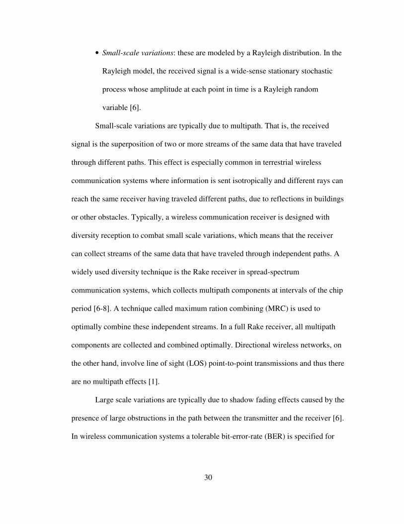
• Small-scale variations: these are modeled by a Rayleigh distribution. In the
Rayleigh model, the received signal is a wide-sense stationary stochastic
process whose amplitude at each point in time is a Rayleigh random
variable [6].
Small-scale variations are typically due to multipath. That is, the received
signal is the superposition of two or more streams of the same data that have traveled
through different paths. This effect is especially common in terrestrial wireless
communication systems where information is sent isotropically and different rays can
reach the same receiver having traveled different paths, due to reflections in buildings
or other obstacles. Typically, a wireless communication receiver is designed with
diversity reception to combat small scale variations, which means that the receiver
can collect streams of the same data that have traveled through independent paths. A
widely used diversity technique is the Rake receiver in spread-spectrum
communication systems, which collects multipath components at intervals of the chip
period [6-8]. A technique called maximum ration combining (MRC) is used to
optimally combine these independent streams. In a full Rake receiver, all multipath
components are collected and combined optimally. Directional wireless networks, on
the other hand, involve line of sight (LOS) point-to-point transmissions and thus there
are no multipath effects [1].
Large scale variations are typically due to shadow fading effects caused by the
presence of large obstructions in the path between the transmitter and the receiver [6].
In wireless communication systems a tolerable bit-error-rate (BER) is specified for

31
large scale variations. Based on the tolerable BER, a minimum received signal power
is required to account for the signal fades and guarantee the specified BER.
In directional wireless communications, large scale signal variations are quite
important and are mainly due to atmospheric turbulence. This effect is especially
strong in FSO links. Optical turbulence is caused almost exclusively by temperature
variations in the atmosphere, resulting in the random variations of refractive index.
An optical field propagates through the atmospheric turbulence will experience
random amplitude and phase fluctuations, which will generate a number of effects:
break up of the beam into distinct patches of fluctuating illumination, wander of the
centroid of the beam, and increase in the beam width over the expected diffraction
limit [13-17]. In terms of communications performance, the intensity fluctuations
produced by atmospheric turbulence translate into reduced signal-to-noise ratio
(SNR) and increased link bit-error-rate (BER). In direct-detection FSO systems using
on-off keyed (OOK) modulation, the BER is found to be:
= 0
22
1erfc
2
1SNRBER , (4.1)
where SNR0 is the signal to noise ratio in the absence of atmospheric turbulence,
defined as:
( )
R
kTBPeB
PiSNR
S
S
N
S
42
2
2
2
0
+ℜ
ℜ==
σ, (4.2)
where is is the output signal current from the detector, σN is the noise variance (zero-
mean white Gaussian noise is assumed), Ps is the received signal power, ℜ is the
receiver responsivity, B is the bandwidth, k is the Boltzmann constant, T is the

32
effective noise temperature, and R is the effective resistance of the receiver circuitry
[9]. In Eq. 4.1 the threshold level is set at half the average signal level 2STH ii = .
In the presence of optical turbulence, the signal current is a random variable
NS iii += with mean Si and variance 222
NSi σσσ += . The averaged SNR is given
by:
2
0
26/5
2
2
0
2
2
233.11 I
L
I
i
S
SNRkw
L
SNRiSNR
σσσ
+
+
== ,
(4.3)
where Iσ is the variance of the intensity fluctuations, L the link length and wL the spot
size [15]. Note from Eq. 4.3 that in the presence of atmospheric turbulence the
average SNR is always lower than SNR0. The resulting BER is obtained averaging
Eq. 4.1 over the intensity fluctuation spectrum. This leads to the expression:
( )∫∞
=
0 22erfc
2
1S
s
s
SI diSNRi
iipBER , (4.4)
where pI(i) is the probability density function (PDF) of the intensity fluctuations. A
lognormal distribution is generally used to model pI(i) [15]. Fig. 4.1 shows the
calculations of BER for an FSO system as a function of SNR0, for intensity variance
ranges from 0.001 to 0.5 [15].

33
Figure 4.1: BER of an FSO system at different intensity variance values.
A lot of work has been done to design techniques for mitigating the effects of
optical turbulence. These techniques involve transmitter and/or receiver designs such
as aperture averaging and delay diversity techniques [18-20].
In this dissertation, turbulence-induced fading models for both RF and FSO
technologies are used for link margin calculations. The minimum received power
needed to guarantee a specified link BER is computed based on these models.
In the context of topology control, the most important channel factor to
consider is the path loss. Given the receiver sensitivity and the link margin for
turbulence-induced fading, the transmitted power needed to guarantee that the
received power is above the link margin will depend on the path loss.
In general, path loss is a function of the link distance and the link directivity.
In directional wireless communications, moreover, absorption of the beam by the

34
atmosphere can be important, especially in adverse weather conditions of fog, clouds,
rain, snow, or in conditions of battlefield obscuration [21]. The combined effects of
direct absorption and scattering of electromagnetic radiation can be described by a
single path-dependent attenuation coefficient ( )zα . The power reaching a RX from a
TX can easily be calculated for links without significant turbulence effects. The
received power PR for a RX with receiver area A, coming from a transmitter at range
L and beam divergence angle θ , varies as:
22
2
L
AePP
L
TRπθ
α−= , (4.5)
where PT is the transmitted power, and α in this case is assumed constant along the
propagation path L. This result assumes a directional beam whose beam width at the
receiver is significantly greater than the receiver diameter. Tightly collimated systems
have been proposed [23] for which L
TR ePP α−= .
In this dissertation, atmospheric propagation models for both FSO and RF
communication will be presented. These include attenuation models based on
scattering of electromagnetic radiation by suspended water particles in the form of
fog and clouds, turbulence-induced fading models and directivity-driven free space
path loss. These models are used to extend current wireless channel models in order
to provide a more comprehensive characterization of the wireless channel in
increasingly heterogeneous and dynamic wireless networks. Communication cost in
DWB-based networks will be defined based on the developed models.

35
4.2 Communication cost model
In DWB-based networks backbone nodes use a hybrid communication mode
in order to communicate with both end users and neighbor backbone nodes.
Omnidirectional RF transmissions are used to cover end users at tier 1 of the
architecture while directional wireless communications are used to aggregate traffic
from end users and transport it through the backbone at tier 2 (see Fig. 1.1).
Moreover, directional wireless communications use both RF and FSO technologies to
send information point-to-point without causing interference. Thus, we need to define
a general link cost function for a wireless link (i,j) that takes into account the behavior
of the diverse wireless technologies used in next generation wireless networks
(omnidirectional RF, directional RF and directional FSO).
In this work, we focus on the communications energy used at the wireless
links forming the network and define the general link cost function for a given link
(i,j) as the transmitted power needed at transmitter i in order to guarantee a specified
BER at receiver j:
ij
j
Rij Pu τ⋅= 0 , (4.6)
where j
RP 0 is the minimum received power at node j in order to guarantee the
specified BER and ijτ is the path loss or path attenuation for link (i,j). We refer to
j
RP 0 as the link margin and will be described based on the large scale variations of the
wireless channel in section 4.3. The path loss ijτ for a link (i,j) with distance L
defined as ji RR −=L , where Ri and Rj are the locations of nodes i and j
respectively, is described in terms of two main components:
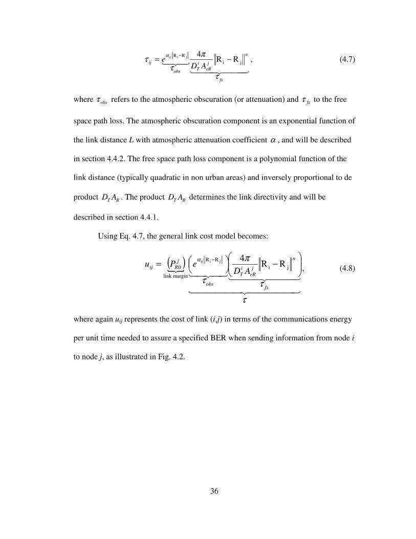
36
444 3444 2143421
fs
n
j
eR
i
Tobs
ijAD
eij
τ
π
ττ
α
ji
RRRR
4ji −=−
, (4.7)
where obsτ refers to the atmospheric obscuration (or attenuation) and fsτ to the free
space path loss. The atmospheric obscuration component is an exponential function of
the link distance L with atmospheric attenuation coefficient α , and will be described
in section 4.4.2. The free space path loss component is a polynomial function of the
link distance (typically quadratic in non urban areas) and inversely proportional to de
product RT AD . The product RT AD determines the link directivity and will be
described in section 4.4.1.
Using Eq. 4.7, the general link cost model becomes:
( )
44444 344444 21
444 3444 2143421
τ
τ
π
τ
α
fs
n
j
eR
i
T
obs
j
RijAD
ePuij
−
=
−
ji
RR
marginlink
0 RR4ji
, (4.8)
where again uij represents the cost of link (i,j) in terms of the communications energy
per unit time needed to assure a specified BER when sending information from node i
to node j, as illustrated in Fig. 4.2.

37
Figure 4.2: Wireless link model parameters.
The link cost function in Eq. 4.8 will be used to characterize the potential
energy of the network system, as stated in Eq. 3.1. Recall that the idea is to abstract
the communications network as a physical system where communication links define
physical interactions between network nodes, which are determined based on the
variation of the potential energy. In the following sections we precisely define the
three main components of the link cost function uij: 1) link margin, 2) atmospheric
attenuation, and 3) free space path loss.
4.3 Turbulence induced fading
Large scale time variations of the received signal intensity in directional
wireless communications are mainly due to atmospheric turbulence. A lot of work has
been done to characterize atmospheric turbulence [13-17], and several techniques
have been developed to mitigate its effects on FSO communication links [18-20]. In
Ri
DT Rj
AR PR0
i j
ijα
L

38
this dissertation we present models that characterize turbulence-induced fading for
both FSO and RF links. These models are used to define the probability density
function (PDF) of the intensity fluctuations pI(i) at the receiver.
In FSO communications a lognormal distribution is generally used to model
pI(i) [15]. One way to measure the strength of atmospheric turbulence is by
examining the variance of the log intensity fluctuations (Rytov variance [19])
described as:
6/116/722 23.1 LkCnR =σ , (4.9)
where 2
nC is the atmosphere refractive index structure parameter, λπ2=k is the
wave number, and L is the propagation length [15]. In terms of this parameter, the
turbulence is called “weak” if 3.02 <Rσ , and “strong” turbulence if 12 >Rσ , although
true strong turbulence may need 252 >Rσ [15].
Fig. 4.3 compares the variances calculated using Fante’s weak and strong
turbulence theories with the Rytov value [19]. It also shows the path of a composite
curve that is predicted to be valid over all turbulence strengths.

39
COMPARISON OF CORRELATION PARAMETER WITH RYTOV VALUESquare root of variances, 863 meters range, 632.8 nonometers
0
1
2
3
0 1 2 3 4 5
Sigma(Rytov)
Sig
ma
(We
ak
) a
nd
Sig
ma
(Str
on
g) Rytov
Weak Theory
Strong Theory
Composite
Weak
Rytov
Strong
Figure 4.3: Weak and Strong Variances compared with the Rytov value [20]. Circles
shown represent the path of a composite curve that is predicted to be valid over all
turbulence strengths.
Note that the “Weak” curve follows the linear variation predicted by the
Rytov variance well up to 3.02 =Rσ . The “Strong” curve is not valid for small values
of 2
Rσ , but should represent expected variances well for 12 >Rσ . The circles in Fig.
4.3 represent a path for a “composite curve” that follows weakσ for small 2
Rσ and then
merges with strongσ for larger 2
Rσ . Such a composite curve demonstrates the increase
in intensity variance that occurs as turbulence increases followed by its saturation at
high levels of turbulence.

40
Under weak turbulence conditions, where the Rytov approximation holds, the
parameter that determines the turbulence strength is the 2
nC value (from Eq. 4.9). Fig.
4.4 shows examples of the Rytov variance in the operating range below 1km for
various turbulence strengths with 2
nC values range from 10-13
to 10-17
, and an optical
wavelength of 1310nm.
Figure 4.4: Rytov variance versus propagating distance (1310nm beam) for different
Cn2 values.
In the case of RF links, which use electromagnetic waves in the millimeter
and microwave region, Clifford and Strohbehn [13] derived a general result for the
amplitude and phase fluctuations, which for the most practical propagation paths of
interest reduce to the formulas presented earlier for optical wavelengths. Thus the

41
Rytov variance as described in Eq. 4.9 will be used to determine the amplitude of
intensity fluctuations for RF links as well. Note that due to the 6/7k dependence, RF
links, which use larger wavelengths than optical links, will experience less intensity
fluctuations and therefore will be more resistant to turbulence effects.
The BER is used as a measure of link performance at the physical layer. A
link is considered feasible for communications if its BER is below a given threshold
(typically 10-9
-10-6
). The link BER can be derived from the signal-to-noise ratio
(SNR) and the probability density function of the intensity fluctuations pI(i) using Eq.
4.4:
( )∫∞
=
0 22erfc
2
1S
s
s
SI diSNRi
iipBER .
From the above equation, the average signal-to-noise ratio SNR required to
guarantee a specified BER can be computed. The required SNR0 can then be found
using Eq. 4.3:
2
0
26/5
2
2
0
233.11 I
L
I SNRkw
L
SNRSNR
σσ +
+
=
Finally, the required average received power PR0 is obtained using Eq. 4.2 as:
ℜ= N
R SNRPσ
00 , (4.10)
where ℜ is the receiver responsivity and Nσ the noise standard deviation.
Based on these models, the minimum received power PR0 for every potential
link in the network can be determined.

42
4.4 Path loss
Directional wireless backbone networks are typically deployed at high
altitudes, where line of sight can be exploited. DWB nodes can be deployed on top of
buildings or other infrastructures, or can be airborne, for example involving UAVs
(Unmanned Aerial Vehicles) at very high altitudes. Thus, the propagation medium
where directional wireless links are going to be deployed typically involves the low
layers of the atmosphere.
Path loss is defined as the attenuation undergone by an electromagnetic wave
in transit between a transmitter and a receiver. The path loss τ for a wireless link can
be derived as the ratio between the transmitted power and the received power:
43421
fs
n
eRTobs
L
R
T LAD
eP
P
τ
π
ττ α 4
== , (4.11)
where obsτ refers to the path loss due to atmospheric obscuration and fsτ to the free-
space path loss. In the following sections we will describe in detail these two main
path loss components.
4.4.1 Free space path loss
The free space path loss measures the attenuation of an electromagnetic signal
that would result from a line of sight path through free space, with no atmospheric
obscuration effects, and it is defined as:
n
eRT
FS LAD
πτ
4= , (4.12)

43
which is a polynomial function of the link distance. The eRT AD
π4 constant is
independent of the nodes’ locations and will be determined by the directivity of the
transmitter antenna DT and the effective receiver area AeR [6].
In this work we are especially interested in studying the effects of different
link directionalities on the free space path loss. The directivity DT of a transmitter is
defined as the ratio of the maximum power density to the power density of a
completely isotropic transmission, as described by:
n
TT
L
PD
π
φθ
4
),( maxΡ= (4.13)
The directivity measures the confinement of electromagnetic energy in the direction
of maximum radiation and can be computed as a function of the solid angle of the
electromagnetic beam as:
Ω
=π4
TD . (4.14)
The solid angle Ω can be computed in spherical coordinates as:
)cos1(2 sin
2
0 0
θπφθθπ θ
−==Ω ∫ ∫ dd , (4.15)
where θ is the half angle beam divergence [6] as illustrated in Fig. 4.5:
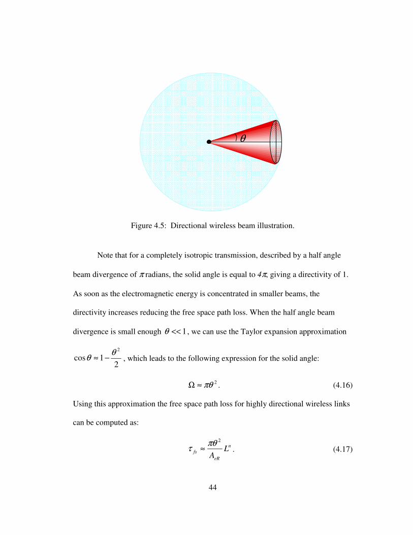
44
Figure 4.5: Directional wireless beam illustration.
Note that for a completely isotropic transmission, described by a half angle
beam divergence of π radians, the solid angle is equal to 4π, giving a directivity of 1.
As soon as the electromagnetic energy is concentrated in smaller beams, the
directivity increases reducing the free space path loss. When the half angle beam
divergence is small enough 1<<θ , we can use the Taylor expansion approximation
21cos
2θθ −≈ , which leads to the following expression for the solid angle:
2πθ≈Ω . (4.16)
Using this approximation the free space path loss for highly directional wireless links
can be computed as:
n
eR
fs LA
2πθτ ≈ . (4.17)
θ

45
In general, the term eRT AD
π4will be computed based on the specific directivity
of the wireless link in consideration, but it will always be a constant independent of
the nodes’ locations. Thus, the free space path loss is modeled as a polynomial
function of the form nxaf ⋅= , where the constant a is determined by the link
directionality and the polynomial order n by the path loss exponent, which typically
takes the value of 2 unless significant obstacles are present such as in urban areas,
where it can take values up to 6 [6].
Thus, assuming a path loss exponent n=2 and clear atmosphere conditions (α
= 0), the general link cost function uij in Eq. 4.8 becomes:
2
ji0 RR4
−
=
j
eR
i
T
j
RijAD
Puπ
, (4.18)
which is a quadratic function of the link distance. As explained in the previous
section, the minimum received power PR0 is determined by the channel fading and the
receiver sensitivity, and will not change with the location of the backbone nodes
(under the assumption that the deployment area of the backbone nodes share the same
turbulence conditions). The eRT AD
π4 constant will also be independent of the
backbone nodes’ locations and will be determined by the directivity of the transmitter
antenna DT and the effective receiver area AR. Thus, the link cost uij as defined in Eq.
4.18 is a function of the form 2xkf ⋅= , which is analogous to the potential energy of
a spring, with spring constant eRT
RAD
Pkπ4
0= and displacement x, the link distance
[53].

46
Using the link cost model form Eq. 4.18, we can model wireless links as
springs which exert attraction forces between network nodes for energy minimization.
The beauty of this model is that given the required received power PR0, and
the effective receiver area AeR, the spring constant is inversely proportional to the
transmitter directivity DT. Thus, directional wireless links which have high
directivities translate into springs with low spring constants, which allow for higher
link distances. On the other hand, omnidirectional wireless links use low directivity
antennas associated with high spring constants that require much more energy to
elongate. This result is very much in accordance with our network architecture, where
directional wireless links are used to connect backbone nodes over large distances,
whereas omnidirectional wireless links are used to connect each terminal node to its
assigned base station (see Fig. 1.1).
As an example, Fig. 4.6 shows three wireless links with different directivity
values and their associated spring models with their respective spring constant values.
In these examples PR0 is assumed to be 1 Watt and AeR 1 m2.

47
Figure 4.6: Spring model for wireless links.
4.4.2 Atmospheric attenuation
The atmospheric attenuation measures the attenuation of the electromagnetic
signal due to the combined effects of absorption and scattering of the beam by the
atmosphere. Atmospheric attenuation is especially important in directional wireless
links deployed at high altitudes and in adverse weather conditions of fog, clouds, rain,
snow, or in conditions of battlefield obscuration [21]. The combined effects of direct
absorption and scattering of electromagnetic radiation are described by an exponential
function of the link distance as:
L
obs eατ = , (4.19)
where the single path-dependent attenuation coefficient ( )zα defines the attenuation
of the signal power as it travels through the atmosphere, caused by the presence of
obscurants such as clouds, rain and snow. Atmospheric attenuation is mainly due to
4/πθ =8/πθ =
πθ = 1=TD
8.6≈TD
3.26≈TD
57.12≈k
85.1≈k 48.0≈k

48
scattering of electromagnetic radiation by the suspended water particles forming such
obscurants.
The cloud attenuation (in dB per unit length) at infrared frequencies (FSO
links) can be described as
SCATFSO e ατ ⋅= )log(10 , (4.20)
where αSCAT is the scattering coefficient and L the link length. The scattering
coefficient is defined as
2
SCAT nQ rα π= , (4.21)
where r is the effective radius of the water particles, n is the number of particles per
unit volume, and Q is the scattering efficiency, which is approximated by a value of 2
for infrared wavelengths and typical cloud water particle sizes [23]. As seen in Eq.
4.21, the scattering coefficient is a function of the size and density of cloud water
particles.
In the case of RF links, the cloud attenuation (in dB per unit length) is related
to the cloud water content using the Rayleigh approximation for small water droplets
[24]:
+
−
=
ε
ε
λρ
πντ
2
1Im
32
34343.0RF , (4.22)
where ν is the cloud liquid content (for cirrus clouds, the ice water content I is used
instead), ρ is the density of water, λ is the wavelength, and ε is the complex dielectric
constant of water.
Table 4.1 shows typical attenuation values for both technologies and for
several cloud types at different altitudes. Typical values for r, n, ν and I, for different

49
cloud types, were obtained from the Bulletin of the American Meteorological Society
[25-26]. The attenuation value is given in dB when going through 1 km of cloud
obscuration. Table 4.1 values show that cloud attenuation is much more significant at
infrared frequencies (FSO links), where scattering of the optical beam by water
particles is dominant.
Layer
Height
(km)
Cloud Type Average
ττττRF
(dB/km)
Average
ττττFSO
(dB/km)
Layer 1 0-1 Fog, Stratus 0.43, 1.4 136, 274
Layer 2 1-2 Stratus,
Cumulus
1.4, 2.8 274, 543
Layer 3 2-6 Altostratus,
Altocumulus
0.98 191
Layer 4 6-8 Cirrus 0.17 122
Table 4.1: Typical cloud attenuation values at different atmospheric layers.
These models are used to compute the path loss for every potential link in the
network. It is important to note that atmospheric attenuation is path dependent. In the
path from a node A to a node B, electromagnetic radiation can encounter different
atmospheric agents giving raise to different attenuation values. Thus, the total path
loss due to atmospheric attenuation for a given link AB needs to be computed by
integrating the path dependent attenuation parameter τ(z) along the link path, as:
∫=B
A
Z
Z
AB dzz)(ττ , (4.23)
where ZA and ZB are the link path components of the location of nodes A and B
respectively, and the integration is over the direction of propagation z. If the

50
obscuration factor remains constant along the path from A to B, Eq. 4.23 becomes a
function of L and the total path loss can be computed as:
+= n
eRT
obs LAD
Lπ
ττ4
log10 , (4.24)
where the link distance L is defined as BA RR −=L , and AR and BR are two or
three-dimensional vectors depending on the topology of the area on which nodes are
distributed.
In our simulations, a finite grid is used in which each cell is assigned a cloud
attenuation value. Free space cells are assigned a value of zero. For that case, the path
loss can be approximated using the following equation:
+=∑ n
eRTi
ii LAD
Lπ
ττ4
log10 , (4.25)
where L is the distance between A and B, τi is the atmospheric attenuation per unit
length for section i of the path AB, Li the section length, and the summation is over
the path AB as shown in Fig. 4.7.
In section 4.5 we describe a methodology to generate dynamic 3D scenarios
including moving cloud layers at different altitudes. The objective is to develop a
simulation tool that would allow 1) the generation of network dynamics in the form of
node mobility, atmospheric obscuration and channel fading, and 2) the
characterization of such scenario in the form of a network cost matrix using the
presented link cost models.

51
Figure 4.7: Illustration of the path loss model for a directional wireless link going
through atmospheric obscuration.
4.5 Dynamic network model
In this section, we present a methodology for the generation and
characterization of dynamic three-dimensional (3D) network scenarios which use the
communication cost models presented earlier to describe the dynamics of DWB-
based network systems.
In order to generate realistic atmospheric obscuration agents in the form of fog
and clouds, digital data sets from the National Climate Data Center (NCDC) at the
National Oceanic and Atmospheric Administration (NOAA) are used to obtain world
wide gridded cloud analysis, including cloud layer data (base, top, type, and amount)
and cloud cover values [27]. Based on this data, cloud layers are generated as the
τ
0
0
0
0
0
0
0
0
0
0
0
0
0
0
0
0
0
0
0
0
0
0
0
0
0
0
0
0
0
0
0
0
0
0
0
0
0
0
0
0
0
0
0
0
0
0
0
0
0
0
0
0
0
0
0
0
0
0
0
0
0
0
0
0
0
0
0
τ τ τ τ τ τ 0
0
0
0
0
0
0
0
0
0
0
0
0
τ τ τ τ τ τ τ τ 0
0
0
0
0
0
0
0
0
0
0
0
τ τ τ τ τ τ τ τ 0
0
0
0
0
0
B
0
0
0
0
0
0
τ τ τ τ τ τ τ τ 0
0
0
0
0
0
0
0
0
0
0
0
0
τ τ τ τ τ 0
0
0
0
0
0
0
0
0
0
0
0
0
0
0
0
0
0
0
0
0
0
0
0
0
0
0
0
0
0
0
0
0
0
0
0
0
0
0
0
0
0 0 0 0 0 0
0 0 0 0 0 0 0 0 0 0 0 0 0 0 0 0 0 0 0 0
A
B

52
superposition of 3D ellipsoidal shapes simulating the presence of atmospheric agents
in the 3D space. Typical wind speed values at different atmospheric layers are used to
move the cloud layers in the 3D space.
Matlab is used to generate these dynamic 3D scenarios. Each snapshot of a
dynamic scenario generated is characterized by an obscuration matrix. The
obscuration matrix is a three-dimensional matrix in which each entry contains the
atmospheric attenuation for a given point in the 3D space. An example of a 2D
obscuration matrix is shown in Fig. 4.7, where all entries with free space are set to
zero and entries containing cloud water particles are set to the specific cloud
attenuation value τobs. The set of obscuration matrices for every snapshot of the
dynamic scenario defines the evolution of atmospheric obscuration over time.
Given the obscuration matrix, the location of the network nodes and the link
directivities, the path loss for every potential link in the network is computed using
Eq. 4.25. Thus, a set of NxN path loss matrices L (one for every snapshot of the
dynamic 3D scenario) is generated in order to define the evolution of the path loss for
every link in the network.
Fig. 4.8 shows an example of a 3D simulation scenario generated in Matlab.
This scenario represents a 16x16x8km 3D space containing 4 cloud layers with
different cloud types at different altitudes and a 10 node directional wireless network
using FSO and directional RF communication technologies. Values for the path loss
(FSO/RF) in dB are shown on every link.
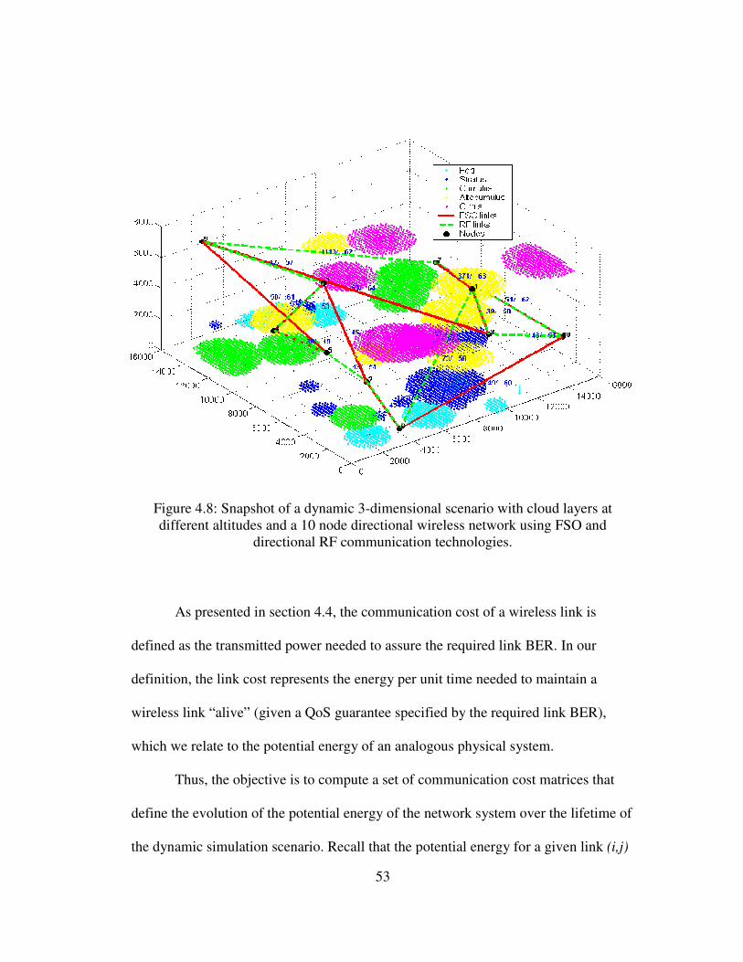
53
Figure 4.8: Snapshot of a dynamic 3-dimensional scenario with cloud layers at
different altitudes and a 10 node directional wireless network using FSO and
directional RF communication technologies.
As presented in section 4.4, the communication cost of a wireless link is
defined as the transmitted power needed to assure the required link BER. In our
definition, the link cost represents the energy per unit time needed to maintain a
wireless link “alive” (given a QoS guarantee specified by the required link BER),
which we relate to the potential energy of an analogous physical system.
Thus, the objective is to compute a set of communication cost matrices that
define the evolution of the potential energy of the network system over the lifetime of
the dynamic simulation scenario. Recall that the potential energy for a given link (i,j)

54
can be computed using Eq. 4.6 as ij
j
Rij Pu τ⋅= 0 . Restating Eq. 4.6 in matrix form we
obtain:
LPU R0= , (4.26)
where U is the potential energy matrix, PR0 the link margin matrix and L the path loss
matrix. The communication cost matix U in dBm is obtained as
L(dB)(dBm)PU(dBm) R0 += , (4.27)
where PR0 is the link margin matrix in dBm and L the path loss matrix in dB. Fig. 4.9
illustrates this process.
Figure 4.9: Modeling the network’s communication cost. The atmospheric conditions
of the 3D space determine the 3D obscuration matrix τ and the 3D turbulence strength
matrix Cn2. Given the location of the network nodes, the NxN path loss matrix L and
the NxN link margin matrix PR0 are obtained from the 3D matrices τ and Cn2
respectively. Finally, the potential energy matrix U, which contains the power needed
at every potential link in the network is obtained using Eq. 4.27 as the aggregation of
L and PR0.
τ
Cn2
L
PR0
U

55
Chapter 5: Topology Reconfiguration
5.1 Introduction
Topology reconfiguration in DWB networks is defined as the process by
which point-to-point links are broken and/or set-up to create a new physical network
topology. Fig. 5.1 illustrates this process:
Initial topology
Router
Router
Router
Router
Topology reconfiguration
Router
Router
Router
Router
Link failures
Router
Router
Router
Router
Initial topology
Router
Router
Router
Router
Router
Router
Router
Router
Router
Router
Router
Router
Router
Router
Router
Router
Topology reconfiguration
Router
Router
Router
Router
Router
Router
Router
Router
Router
Router
Router
Router
Router
Router
Router
Router
Link failures
Router
Router
Router
Router
Router
Router
Router
Router
Router
Router
Router
Router
Router
Router
Router
Router
Figure 5.1: The topology reconfiguration process.
In this context, we define:
• Topology optimization: computation of an optimal topology from global
network knowledge.
• Bootstrapping: initial configuration of a connected topology from
disconnected network nodes with only local network knowledge.
56
5.2 Topology Optimization
5.2.1 Introduction
Topology reconfiguration may be designed to meet multiple objectives such
as minimizing congestion, end-to-end delay or bit-error-rate (BER). Algorithms and
heuristics are used for making efficient decisions about the choice of network
topology to achieve a required level of performance. Fig. 5.2 shows the interaction
between the topology control processes that provide the network with the autonomous
reconfiguration capability.
Most physical layer topology control algorithms for multi-hop wireless
networks attempt to optimize parameters such as power or bit error rate (BER). In
FSO networks the critical factor affecting link performance at the physical layer is the
atmospheric obscuration, which reveals the attenuation of the optical signal caused by
the presence of atmospheric phenomena (clouds, fog, snow, etc) between the nodes
trying to communicate. Thus, in [42], we considered the obscuration minimization
problem.
A cost measure is assigned to every possible link in the network as a function
of the link length and the obscuration factor. Minimum cost graph algorithms
techniques are then used to construct optimized topologies. Constraints are imposed
on the node degree (due to the limitation on the number of transceivers) and the
network connectivity (specifically we will impose the network to be bi-connected,

57
which assures the existence of a communication path between any two nodes in the
network even after a single link break).
Link state examination: Link state is highly dynamic. Adverse weather conditions
such as clouds, fog and snow may obscure optical links causing performance
degradation manifested by increased BER, transmission delays, congestion, etc.
These effects are even greater when allowing mobility of nodes. In such a
dynamic environment, nodes should be continuously monitoring their link states
and local topology information.
Collection of link state information: Upon degradation, link state information is
reported to a designated node in order to keep track of the dynamics of the whole
network and determine whether a topology change is needed.
Topology solution computation: If a new topology needs to be computed, the
challenge is to develop efficient algorithms to find the optimal topology meeting
a given objective while satisfying connectivity constraints. We have developed
approximation algorithms to solve the problem in polynomial time as these
algorithms must be scalable and be executed with low complexity to avoid
significant loss of data. This issue becomes critical due to the extremely high data
rates carried in optical wireless networks.
Distribution of topology solution: The new topology is sent to every node in the
network in order to undergo reconfiguration.
Deployment/Reconfiguration: The deployment of the new topology takes place.
Beam steering plus pointing-acquisition and tracking techniques are used in order
to physically redirect the optical beams and quickly form a new topology [29].
Figure 5.2: Autonomous reconfiguration processes.
Link State Examination
Collection of Link State Information
Distribution of Topology Solution
Solution Computation
Deployment/Reconfiguration

58
Topology optimization problems are typically NP-Complete and heuristics are
needed in order to achieve scalable near-optimal solutions. Heuristics for topology
optimization can be broadly classified into two categories as link insertion and link
deletion. Link insertion heuristics insert links according to some sequence whenever
interfaces are available. In link deletion heuristics the starting point is a maximally
connected graph, and links are removed according to some sequence until no node
has more links attached to it than it its number of interfaces.
Two centralized approaches to create an FSO topology with strong
connectivity and short diameter with uniform degree bounds were presented in [43].
One is based on link deletion, and the other is based on link insertion. Their work
does not take into account link cost and does not assure bi-connectivity. In [44],
heuristics for minimizing BER and congestion, with bi-connectivity constraints, are
described. All of them are based on link insertion.
In [42] we presented two heuristics for building minimum cost bi-connected
topologies in the case of 2-degree (ring) networks as well as for 3-degree networks.
All of them fit in the category of link insertion. The heuristics for ring networks were
based on the Spanning Ring methodology presented in [44]. For 3-degree networks a
new heuristic, 3-MST + Bridge Covering, was described, which achieves a closer to
optimal solution with a slight increase in complexity compared to the 3-degree
heuristic presented in [44].
5.2.1 Problem Statement
The topology optimization problem is stated as follows:

59
• Given: The network cost matrix C representing the cost of all possible
links in the network.
• Objective: Find the network topology T minimizing the aggregate network
cost F.
• ∑∑= =
=N
i
ij
N
j
ijij cbbF1 1
)( , where
=
∈
=
),(link ofcost
o.w 0
if 1
jic
T(i,j)b
ij
ij
(5.1)
• Constraints: node degree (which must not exceed the number of directional
transceivers per node) and edge bi-connectivity (the network must remain
connected even after a single link break).
Note that in the topology optimization problem above, the cost matrix C is
given and the optimization is performed over the ijb variables, which determine the
connections between backbone nodes. The topology optimization problem is actually
an instance of the general energy minimization problem stated in Eq. 3.3:
∈
=
+
⋅= ∑∑∑
== =
o.w. 0
if 1 s.t.
)r,R()R,R()R,...,R,(min1
)h(
1
ji
1
N1
T(i,j)b
uubbU
ij
M
k
kk
N
i
N
j
ijij η
.
Note that when the location of the backbone nodes N1 R,...,R is given and the
optimization is done over the backbone connectivity variables bij, the network
coverage term G is fixed and does not affect the optimization process. Only the
backbone connectivity term F is considered and 3.3 reduces to:

60
∈
=
=∑∑= =
o.w. 0
if 1 s.t.
)R,R()(min1
ji
1
T(i,j)b
ubbU
ij
N
i
N
j
ijij
, (5.2)
where now the energy function U is just the backbone connectivity term F. The
topology optimization problem is thus a connectivity optimization problem
formulated as an integer programming problem.
In our approach, a weighted graph is considered as the abstraction of the
network. A weighted graph G = (V, E) is a group of |V| vertices connected through |E|
weighted edges. The vertices represent the nodes in the network and the edges the
links between them. The weight of an edge describes the cost associated with the link
represented by that edge. The problem becomes that of finding sub-graphs with
minimum total cost while satisfying connectivity constraints. Specifically, heuristics
have been developed to solve the problem of finding the minimum cost ring topology
(suitable when nodes have 2 optical transceivers), which is NP-Complete [40]. Also,
the problem of forming a bi-connected topology when nodes are allowed to have up
to 3 optical transceivers has been considered. In this case heuristics have been
developed to find a 3-degree minimum spanning tree (3-MST) (NP-Complete [40]),
and augmenting the tree to achieve bi-connectivity (also an NP-Complete problem
[40]).
5.2.2 Heuristics for ring networks
When all network nodes have 2 optical transceivers the only possible bi-
connected topology is a ring. The problem is to find the minimum cost ring topology.

61
In graph algorithms theory, this is equivalent to the “traveling salesman problem”,
which is known to be NP-Complete [40]. A simple heuristic called Spanning Ring
(SR) was introduced in [44]. This heuristic keeps forming a simple path by adding
edges in increasing order of cost and closes the path into a ring when all nodes are
included. SR uses Prim’s MST algorithm [41] with the additional constraint of the
node degree being equal to 2, which indeed builds a close-to-minimum spanning ring.
Its running time complexity is O(E log V) (the complexity of Prim’s MST algorithm
[41]). Observing that |E| = O(V2) (the number of all possible links in the network
grows with the square of the number of nodes), we can re-state the complexity of SR
as O(V2
logV). This heuristic follows a greedy approach, that is, it makes locally
optimal choices in the hope that this choice will lead to a globally optimal solution.
The main problem is that there may be conditions where no feasible link can be added
to the path in either direction, and, thus, a feasible ring topology cannot be found.
In order to overcome this problem, a new heuristic was developed,
Reconfigurable Spanning Ring (RSR). This heuristic forms a simple path by adding
least cost links, but when the path cannot be extended in either direction, an attempt is
made to close it in a temporary ring, either by the path endpoints or by breaking an
already set-up link. Then, the ring is opened into a new simple path and an attempt is
made to extend it again. The process continues until all nodes are included. The
procedure is described as follows:
• Sort links in increasing order of cost.
• While not all nodes included,
o Add links to path in increasing order of cost.
o If the path cannot be extended in either direction,
Reform path:
• If a connection between the path endpoints is possible, make it.

62
• Else,
o Sort links in the temporary path (excluding both path-end
links) in increasing order of cost.
o Break highest cost link and attempt to close the path into a
temporary ring by connecting the path endpoints to the
broken link endpoints.
o If no feasible connections exist, break next highest link and
make a new attempt to form a temporary ring.
• If a temporary ring could be formed, break next highest cost
link to open the ring into a new simple path.
• Else, no feasible solution.
The possibility of breaking already set-up links and reconfiguring the path as
it is formed, gives the heuristic more flexibility to find a feasible solution. Intuitively
we should expect additional time complexity as the algorithm needs to search for
feasible ways to reform the path when getting into an infeasible situation (no feasible
links can be added to extend the path). Specifically, the reforming process adds to the
time complexity of the heuristic, in the worst case (that is when reform path needs to
be executed at every step, and all intermediate path links need to be examined before
a temporary ring can be formed), an O(V2 logV) factor. This is because for each
reform path call we need to sort the edges in the temporary path, which takes O(i
logi) time (heapsort algorithm [41] is used), where i is the number of edges in the
temporary path. In the worst case, we will have to reform the path for every link
addition. Thus, the complexity of RSR is given by
).log(
)log(
)!log(loglog
2
1 1
VVO
VVOV
VViViiV
i
V
i
=
=
=≤∑ ∑= =
The overall running time of the RSR heuristic is therefore O(V2 logV + V
2
logV) = O(V2 logV). Despite the additional time used by the reforming process, RSR

63
maintains the same polynomial complexity and provides higher efficiency in finding
feasible minimum cost ring topologies.
A simulation was developed to measure the performance of these heuristics.
The simulation involved multiple runs in which the heuristics attempt to configure a
minimum cost topology for a particular network scenario. Fig. 5.3 shows the
performance of both heuristics. The dashed line shows the network cost for the
topologies obtained using SR. The solid line represents the network cost for the
topologies obtained by RSR. The white circles represent the instances where SR does
not achieve a feasible solution (some of the active links have higher cost than the link
cost threshold). In most of those cases, the RSR heuristic is able to find a feasible
solution by reforming the temporary path. The black dots show the situations where
not even RSR is able to configure a feasible topology.
Time complexity was also measured for both heuristics. Experiments were run
in which the average time taken for computing a new topology was measured
(average over a 100 runs in different scenarios) as a function of the number of nodes,
for both heuristics. Fig. 5.4 shows the reconfiguration time for 8 to 60 nodes. As
expected, RSR spends more time on average, but both heuristics follow a polynomial
pattern. For a 30 node network, SR took an average of 1.7 ms, while RSR took almost
4 ms to compute the topology.
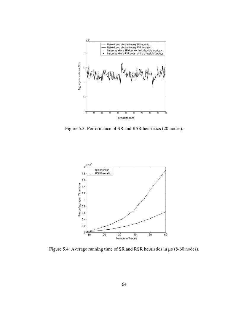
64
0 10 20 30 40 50 60 70 80 90 1000
0.5
1
1.5
2
x 104
Simulation Runs
Ag
gre
ga
te N
etw
ork
Co
st
Network cost obtained using SR heuristicNetwork cost obtained using RSR heuristicInstances where SR does not find a feasible topologyInstances where RSR does not find a feasible topology
Figure 5.3: Performance of SR and RSR heuristics (20 nodes).
10 20 30 40 50 600
0.2
0.4
0.6
0.8
1
1.2
1.4
1.6
1.8
2x 10
4
Number of Nodes
Re
co
nfig
ura
tio
n T
ime
in u
s
SR heuristicRSR heuristic
Figure 5.4: Average running time of SR and RSR heuristics in µs (8-60 nodes).

65
The Branch Exchange algorithm provides a way to incrementally move
towards the optimal topology from an already established one. Branch exchange is a
brute force approach that checks all possible configurations obtained by exchanging
one or more links of the initial topology. The k-link Branch Exchange algorithm
checks all configurations that can be formed by exchanging k links of the initial
topology and keeps the one that meets the given objective (in our case, the one with
minimum aggregate cost).
In the case of rings, at least 2 links must be exchanged by corresponding 2
new links to find a new ring topology. Thus the 2-link Branch Exchange algorithm
can be used to find the ring topology with the minimum aggregate cost, differing
from the existing topology by 2 links. The pseudo code for the 2-link Branch
Exchange algorithm is as follows:
• Find all possible link pairs that can be exchanged by new link pairs
to obtain another ring topology.
• Get the current link pair and remove both links.
• If the 2 links to be added in order to form the new ring topology
have lower cost than the link cost threshold,
o Add the 2 new links.
o Compute the new aggregate network cost.
• Go to next link pair.
• If all link pairs are finished, stop.
• Find the minimum aggregate network cost and take the
corresponding link pair.
• Exchange it for the new link pair.
Since there are 2
)3( −NN (N=|V|, the number of nodes) possible branch
exchanges to obtain a new ring topology, which differs by two links from the existing
ring topology, the time complexity of the 2-link Branch Exchange algorithm is O(V2).

66
After a link pair is exchanged by the corresponding new link pair, the Branch
Exchange algorithm can be executed again upon this new topology to gain further
improvement. Multiple iterations of the Branch Exchange algorithm successively find
topologies with better performance (lower aggregate cost) at the expense of increased
run time complexity.
In our simulation the 2-link Branch Exchange algorithm was applied to the
topologies obtained by RSR in order to gain further improvement and achieve closer-
to-optimal topologies. Fig. 5.5 shows how most of the performance improvement
achieved by the Branch Exchange algorithm is accounted in the first iteration.
Improvement increases with network size. Performance improvements range from 1%
to 5% for networks of 10 to 20 nodes. This suggests that there is little room for
improvement for the topologies obtained by RSR.
10 12 14 16 18 200
1
2
3
4
5
6
Number of Nodes
% R
ed
uctio
n in
Ne
two
rk C
ost
Iteration1
Iteration2
Iteration3
Iteration4
Figure 5.5: Average cost reduction with successive Branch Exchange iterations.

67
In order to determine the effectiveness of our heuristics we compared our
results to the optimal solutions found via integer programming. The integer
programming formulation for the optimal solution, in the case of ring networks, is as
follows:
min ∑∑= =
=N
i
ij
N
j
ijcbF1 1
, where
=
∈
=
),(link ofcost
o.w 0
if 1
jic
T(i,j)b
ij
ij
s.t.
∀=
∀=
∑
∑
=
=
N
j
ij
N
i
ij
ib
jb
1
1
,1
,1
degree constraints
≠∀≠∀−−≤+−
≠∀≤≤
=
1j 1i ),1)(1(1
1,2
11
ijji
i
bNuu
iNu
u
sub-tour
elimination
Constraints
Fig. 5.6 shows the histogram of the optimality gap for our best performance
heuristic for ring networks, RSR+BE [42].
Figure 5.6: Histogram of the optimality gap for RSR+BE heuristic.
0 1 2 3 4 5 6 7 8 90
5
10
15
20
25
optimality gap(%)
freq
ue
ncy

68
5.2.3 Heuristics for 3-degree networks
The possibility of having 3 optical transceivers per node allows greater
flexibility and reduced complexity in forming or configuring networks with higher
connectivity. Assuming every node has 3 optical transceivers and the cost matrix is
known, the problem is to find the minimum cost bi-connected topology.
To solve this problem, a 2-step approach is proposed:
• Form a minimum connectivity graph, i.e. a spanning tree, with minimum
cost.
• Augment the spanning tree to achieve bi-connectivity, also with minimum
cost.
It is known that the problem of finding an MST when the node degree is
bounded (which is the case as every node has 3 transceivers) is NP-Complete [40].
The 3-MST heuristic is used for step 1, which builds a close-to-minimum spanning
tree with 3-degree bound. In this case we use Kruskal’s MST approach [41], which
picks edges in increasing order of cost independently of the already selected edges
(Prim’s approach makes sure the edges are added to the set of already selected edges).
The time complexity is also O(E logV) [41]. Again |E| = O(V2), therefore 3-MST
takes O(V2 logV) time.
Step 2 is a bi-connectivity augmentation problem, which is also known to be
NP-Complete [40]. The heuristic developed, Reconfigurable Spanning Path (RSP)
uses RSR methodology to connect the nodes with degree 1, i.e. with just one active
link. The only difference is that we do not need to form a ring, as a simple path
connecting 1-degree nodes is sufficient to achieve bi-connectivity [41]. The heuristic

69
thus stops when all 1-degree nodes are connected through a simple path. The time
complexity is the same as for RSR heuristic, i.e. O(V2 logV). Thus “3-MST + RSP”
runs in O(V2 logV + V
2 logV) = O(V
2 logV) time. The problem of RSP is that we
won’t always be able to find a feasible path connecting 1-degree nodes. These nodes
are the leaves of the tree constructed in step 1 (which may well be further apart) and
connecting them through a path won’t always be a good solution. A better approach
should add edges between nodes with open interfaces (1 and 2-degree nodes) and stop
as soon as bi-connectivity is achieved. We present the Bridge Covering (BC)
heuristic, which is based on the just stated idea. Before going into the details of the
heuristic we shall introduce the concept of a bridge in a graph, which is critical in our
objective of achieving bi-connectivity. A bridge is an edge in a graph upon the
removal of which, the graph becomes disconnected. Recall that a bi-connected graph
is a graph that will remain connected after any single link break.
Following theorems connect the bridge concept with graph connectivity [41].
Theorem1: If a graph is said to be bi-connected, the graph contains no bridges.
Proof: If a graph is bi-connected we can remove any single edge of the graph
and the graph will remain connected. Therefore a bi-connected graph cannot contain
any bridge.
Theorem2: If a graph is said to be a tree, all the edges of the graph are bridges.
Proof: Since a tree is a connected graph with no cycles, by a single removal of
any of its edges, the graph becomes disconnected. Therefore all the edges of a tree are
bridges.

70
Based on theorem 2 we know that all the edges in the tree obtained in step 1
are bridges. The idea is to add edges to the tree in such a way that for each link
addition, we cover as many bridges as possible. By theorem 1 we know that when all
bridges are covered, the graph is already bi-connected. It is important to remind that
our objective is to find a bi-connected graph with minimum cost, thus the cost of the
edges to be added should be still taken into account. The BC heuristic adds edges in
increasing order of “bridge covering capability”, until the final graph contains no
bridges. The “bridge covering capability” metric is defined so that both, the number
of bridges covered and the link cost, are taken into account. Specifically, the “bridge
covering capability” of a particular edge e is defined as the sum of the cost of all the
bridges covered upon the addition of e minus the cost of e. The pseudo code for the
BC heuristic is as follows:
• Build a potential link set with all possible links between nodes
with open interfaces (nodes with degree 1 or 2).
• Build a bridge set for each of the potential links containing the
bridges which would be covered upon the addition of the potential
link to the tree.
• Compute the bridge covering capability for each potential link.
• Sort links in the potential link set in increasing order of bridge
covering capability.
• Add the link with highest bridge covering capability.
• Update the potential link set, the corresponding bridge sets, and
bridge covering capabilities.
• If no bridges left,
o End.
• Else,
o Go to step 3.
The critical task in the BC heuristic is to build and update the bridge sets.
Initially we need to run BFS (Breadth First Search algorithm) [41] for every potential
link in order to build their bridge sets. BFS on a tree takes O(V) time and we have

71
O(E)= O(V2) potential links. Therefore step1 takes O(V
3) time. For the update steps,
we need O(E) = O(V2) updates after each link addition. Each update takes O(V) time
and there are O(V) link additions. Thus the updating process takes O(V4) time. The
dominating factor is the updating process, which makes BC to run in O(V4) time. The
whole “3-MST + BC” heuristic runs in O(V2
logV + O(V4)) = O(V
4) time.
The same simulation methodology described in section 3 was used to measure
the performance of the 3-degree heuristics. Results are shown in Figs. 5.7 and 5.8. As
in the case of ring topologies the graph in Fig. 5.7 shows the network cost after
configuring an optimized topology by using “3-MST + RSP” (dashed line) and “3-
MST + BC” (solid line) heuristics. The experiment shows how “3-MST + BC”
obtains closer-to-minimum cost bi-connected topologies at the expense of a higher
degree polynomial time complexity (Fig. 5.8). The average running time of 3-degree
heuristics went into a few seconds range for very large networks (about 13 seconds
for 60 nodes) but it was still less than 100 ms for 25 node networks. Also, BC is
shown to be much more efficient in achieving bi-connectivity than RSP. The white
dots in Fig. 5.7 show the instances where RSP fails to achieve a feasible path
connecting 1-degree nodes, thus failing to achieve a bi-connected graph. In those
cases BC finds a feasible set of edges to be added to the tree and achieve bi-
connectivity. The black dot shows that for a particular scenario in our simulation not
even a feasible tree could be obtained.

72
0 10 20 30 40 50 60 70 80 90 1000
0.5
1
1.5
2
2.5x 10
4
Simulation Runs
Ag
gre
ga
te N
etw
ork
Co
st
Network cost obtained using 3-MST + RSPNetwork cost obtained using 3-MST + BCInstances where a just connected topology is obtainedInstances where no feasible connected topology is obtained
Figure 5.7: Performance comparison of 3-degree heuristics (20 nodes).
10 15 20 25 30 35 40 45 50 55 600
2
4
6
8
10
12
14x 10
6
Ru
nn
ing
Tim
e in
us
Number of Nodes
3-MST + RSP3-MST + BC
Figure 5.8: Average running time of 3-degree heuristics (8-60 nodes).

73
5.3 Bootstrapping
In this section, we address the problem of initial configuration of a directional
wireless network topology, which is referred to as the bootstrapping problem. In this
context, nodes are initially disconnected and only know about potential neighbor
connectivity. Nodes therefore need to coordinate their local decisions and actions to
collectively establish a connected topology. An efficient solution to the bootstrapping
problem requires the design of a self-organized system in which the emergence of a
system-wide adaptive structure such as global network connectivity is achieved
through local interactions between individual entities (network nodes).
Our work on topology optimization [42] assumes the existence of a connected
topology. The objective is to dynamically evaluate the current topology and
reconfigure amidst degradation. Such an assumption makes the implementation of a
centralized system very suitable, as overall network information can be used to
efficiently obtain close-to-optimal solutions while avoiding agreement, coordination
and synchronization problems. A Designated Topology Control Node (DTCN) [3] is
responsible for gathering overall network information, evaluating the current
topology, deciding upon reconfiguration and computing a new optimized topology.
Moreover, the available high-bandwidth connectivity allows overcoming the
scalability and response time limitations of centralized systems in low-bandwidth,
unreliable networks.
The objective in bootstrapping is to provide fast initial connectivity rather
than optimizing an existing topology. The problem of initially configuring a network
topology is distributed in nature as nodes only know about potential neighbor

74
connectivity and need to coordinate their local decisions to collectively set up an
initial connected topology.
A complete bootstrapping model requires the design of algorithms and
protocols for:
• Determining the connections to be formed until a connected network is
obtained.
• Exchanging information between nodes in the network.
• Guaranteeing coordination and synchronization.
The limitation on the number of transceivers per node imposes a constraint on
the degree of the network topology being formed. The problem of achieving fast
connectivity with limited number of transceivers per node can be modeled as the
Minimum Degree Spanning Tree (MSDT) problem, which is known to be NP-
Complete. In our previous work, a distributed approximation algorithm which
constructs a spanning tree with maximal node degree at most one larger than that in
the optimal solution was developed [41]. This work provides a bottom-up
methodology to iteratively establish connections until a tree topology is formed, but
does not address the problems of information exchange and synchronization which
are essential in guaranteeing the efficient formation of a connected topology.
In [52] we presented the design, implementation and evaluation of a hybrid
distributed/centralized bootstrapping model for directional wireless backbone
networks. Our approach uses the advantages of a centralized computation and
communication model as soon as high-bandwidth connectivity is available between a
given set of nodes. The bootstrapping process iteratively transforms a completely

75
disconnected distributed network system into a set of connected centralized
components, until a single connected network with a unique DTCN is formed. Our
model uses a bottom-up distributed algorithm to determine connections between
connected components, and adds the required communication and synchronization
mechanisms in order to assure the efficient emergence of network connectivity from
local interactions between connected components.
We have designed a process model in the form of a finite state machine,
which can be integrated in any directional wireless network model in order to provide
the bootstrapping functionality. Simulation experiments were run to test the
efficiency and scalability of our model for different network systems, with varying
size and signaling data rate.
Fig. 5.4 shows the average total delay for bootstrapping directional wireless
networks of 10 to 100 nodes, for different signaling data rates. As expected, the total
delay increases when decreasing the signaling data rate, but the linear time
complexity is preserved, verifying the scalability of our model.

76
10 20 30 40 50 60 70 80 90 1000
5
10
15
20
25
30
35
total number of nodes
de
lay
(s
ec
)
total delay (baseline model)
total delay (500 bps signaling rate)
total delay (200 bps signaling rate)
total delay (100 bps signaling rate)
Figure 5.9: Average total delay of the bootstrapping process.

77
Chapter 6: Mobility Control
6.1 Introduction
As seen in Chapter 5, topology reconfiguration processes allow dynamic
network performance optimization by physically changing directional wireless links
among network nodes. This process involves temporary loss of data due to the
unavailability of several source-to-destination paths during the reconfiguration
process. In directional wireless networks, the degree constraints imposed on the nodes
imply that during a topology change, unwanted links have to be removed before new
links can be created. Whenever this is the case, the network topology will be in a
transient state after the removal of unwanted links and before the establishment of
new links. This transient state could exist for a small time interval, but it nevertheless
exists and results in suboptimal network performance during this time.
Whenever topology reconfiguration cannot improve network performance due
to a high reconfiguration cost, the physical DWB configuration can be adjusted by
repositioning mobile base station nodes. Mobility control allows adjusting the
backbone topology without breaking point-to-point links and thus avoiding temporary
loss of data.
Recall that in our proposed architecture, a set of dynamic “service demand
clusters” are to be connected by a set of directional wireless backbone nodes with
limited coverage range (dotted circles Fig. 6.1). A service demand cluster is

78
essentially a connected set of hosts or terminals which demand for broadband
connectivity (hexagons in Fig. 6.1).
In this architecture, a communication between two terminal nodes takes place
by a multi-hop transmission scheme over the wireless nodes until the traffic of the
source reaches one of the backbone nodes, then it travels over the backbone network
until it reaches a backbone node which is close enough to the intended destination,
and finally it travels over a few wireless nodes until it reaches its destination. Our
problem is to find the optimal locations of the backbone nodes such that two main
objectives are maximized: network coverage and backbone connectivity. A point that
makes our problem distinct from traditional facility location problems is the fact that
we need to make the backbone connected through FSO and/or RF links. This implies
that backbone nodes need to stay within FSO/RF communication range and imposes
further constraints than just covering the service demand areas. As a consequence,
providing coverage to service demand areas and maintaining strong backbone
connectivity results in a multi-objective optimization problem with two competing
objectives. Maximizing backbone connectivity involves bringing backbone nodes
together, which leads to strong backbone connectivity, but may incur in low network
coverage (Fig. 6.1b). On the other hand, maximizing coverage involves spreading
backbone nodes over to service demand areas, which may lead to a weaker (i.e.,
lower connectivity) backbone configuration (Fig. 6.1a).

79
Figure 6.1: Trade-off between network coverage and backbone connectivity.
6.2 Potential energy minimization
This work proposes a novel approach to solve this problem by formulating it
as an energy minimization problem in which the network is modeled as a system of
particles in a potential field. The idea is to characterize the DWB configuration with a
cost function that mimics the potential energy of an analogous particle system.
Energy functions are typically convex, and thus suitable to minimize. Moreover,
being able to characterize network configurations with energy functions allows the
design of self-organized network systems which autonomously achieve energy
minimizing configurations driven by local forces exerted on network nodes. Forces
between nodes are defined based on network connectivity. Attraction forces are
a) High coverage, low connectivity b) Low coverage, high connectivity
c) Joint coverage-connectivity optimization

80
defined between neighbor backbone nodes (for backbone connectivity) and between
each backbone node and the terminals within their respective coverage range (for
network coverage). The effects of the host layer (cluster mobility) and of the
environment (atmospheric turbulence and obscuration) are modeled as external forces
changing the potential energy of the network system. Mobility control algorithms are
designed to autonomously readjust the DWB physical topology based on resulting
forces to achieve energy minimizing configurations.
Physical systems naturally react to minimize their potential energy and
thereby increase their robustness. Internal forces are responsible for bringing the
network to an equilibrium condition where the total energy is minimized. Our
approach models network control strategies as internal forces minimizing the energy
of the network system. In this work, we present algorithms and protocols for mobility
control that adjust the location of backbone nodes by computing internal forces at
each backbone node as negative energy gradients. We show how the network can
autonomously achieve energy minimizing configurations driven by local forces
exerted on network nodes. The beauty of this physical energy model is that very
complex systems can be characterized with continuous and convex energy functions
which take into account the heterogeneity of the network system. We also show how
the use of mobility control strategies that minimize the energy of the network system,
ensure desirable network properties such as coverage, connectivity and power
efficiency.

81
6.3 Coverage and connectivity optimization
Assume we have a network of N backbone nodes and M end terminals or hosts
located in a geographical space 3R∈A . The end hosts are at locations M21 r...,r,r in
the network, in which ),,(ri iii zyx= represents the location of the ith
end host in A.
Similarly, the backbone nodes are at locations N21 R...,R,R in the network, in which
),,(R j jjj ZYX= denotes location of the jth
backbone node in A. Each backbone node
provides coverage to a group of end hosts in its proximity. In this scheme, a host s
communicates with another host d in the following way: host s transmits its
information to the closest backbone node; then the traffic traverses through the
backbone network until it reaches the backbone node that is closest to the destination.
Finally, the backbone node that is closest to the destination transports the traffic to the
host d. As it can be observed, this scheme is based on two properties: first, the end
hosts need to be well covered by the backbone nodes, and second, the backbone
nodes must have good connectivity among themselves. We describe both aspects in
our model in terms of the following two cost metrics:
– Coverage cost: takes into consideration the cost of covering the end hosts
by the backbone network. This component of cost is defined as a function
of the communications energy needed in order for the end hosts to
communicate with their closest backbone node. The more the energy
required, the higher the coverage cost. Assume that h(k) represents the
index of the backbone node that provides coverage to the end host node k.

82
Apparently, we have Nkh ≤≤ )(1 . Now, we define the following form of
coverage cost:
∑=
=M
k
kkuG1
)h( )r,R( , (6.1)
where G represents the coverage cost and it is computed as the summation
of the energy stored in the wireless links connecting each end host to its
closest backbone node.
– Connectivity cost: considers the cost of maintaining the backbone nodes
connected. In the simplest form, backbone nodes may be connected
forming a chain topology, which implies that a chain of links starts from a
backbone node and passes through all the other backbone nodes. In many
practical applications such a simple graph is vulnerable to link failures; if
a single link fails the network becomes disconnected. In practice, it is
desirable to achieve some degree of fault tolerance by superimposing a
redundant connectivity graph among the backbone nodes. Samples of such
connectivity patterns include ring topologies, or k-connected graphs (the
graphs for which there are k disjoint paths between every arbitrary pair of
backbone nodes). For a given connected topology, the connectivity term of
the cost function models the energy used by the backbone network to keep
its nodes connected. Similar to the coverage cost, we define the
connectivity cost as follows:
∑∑= =
=N
i
N
j
ijubF1
ji
1
)R,R( , (6.2)

83
in which F represents the connectivity cost and it is computed as the
summation of the energy stored in the links forming the backbone
topology.
Based on the above cost components, we define the following composite cost
function:
+
⋅=+⋅= ∑∑∑
== =
M
k
kk
N
i
N
j
ij uubGFU1
)h(
1
ji
1
)r,R()R,R(ηη . (6.3)
Note that the cost function above U integrates both coverage and connectivity
cost terms and represents the total energy usage in the network system.
Thus, in this dissertation, the mobility control problem is formulated as an
energy minimization problem, as follows:
∈
=
+
⋅= ∑∑∑
== =
o.w. 0
Tj)(i, 1 s.t.
)r,R()R,R()R,...,R(min1
)h(
1
ji
1
N1
ij
G
M
k
kk
F
N
i
N
j
ij
b
uubU
44 344 21444 3444 21
η
. (6.4)
Note that in this case the backbone topology T (bij variables) is given and the
optimization is performed over the location of the backbone nodes )R,...,R( N1 .
Changing the location of the backbone nodes changes the link cost function uij for
both backbone-to-backbone and backbone-to-terminal links. The objective is to find
the location of the backbone nodes that jointly optimizes network coverage and
backbone connectivity by minimizing the total energy of the network system.
The form of the above energy function depends on the communication cost
model. As seen in section 4.1.3, the cost of a wireless link (i,j) is defined as the

84
communications energy per unit time used to send information at a specified BER
between node i and node j, and it is described in terms of three main components: the
link margin PR0, the atmospheric attenuation obsτ and the free space path loss fsτ :
( )
44444 344444 21
444 3444 2143421
τ
τ
π
τ
α
fs
n
j
eR
i
T
obs
j
RijAD
ePuij
−
=
−
ji
RR
marginlink
0 RR4ji
.
Note that the link energy function uij is the product of a polynomial and an
exponential function of the link distance and thus is convex. In the following sections,
we will introduce reasonable assumptions regarding atmospheric obscuration and free
space path loss for the link cost function uij that will lead to different energy models,
always maintaining the convexity property of the energy function. The mobility
control algorithms developed will differ under the assumptions adopted, but the
general methodology will remain the same. Forces will be computed at each
backbone node as the negative energy gradient at the backbone node’s location,
which will drive their mobility and thus the network topology. In sections 6.3 and 6.4
we present the general force-driven mobility control methodology that will apply on
all scenarios and for all energy models developed. In section 6.5 we present results
for the specific case of clear atmospheric conditions in which the network system is
shown to behave like a spring system. In section 6.6 the effects of atmospheric
obscuration are introduced. In section 6.7 the model is extended to include power
limitations arising in practical scenarios.

85
6.4 Force-driven mobility control
Our approach to solve the optimization problem described in Eq. 6.4 is to use
iterations on the placement of the backbone nodes. In each iteration, forces are
computed at each backbone node that determine the backbone nodes’ relocation
directions. In the following section, we define the notion of the force acting on a
communications network node based on the gradient of the energy function U with
respect to the node’s location.
6.4.1 Communication-defined forces
Using Eq. 6.3 we can compute the gradient of the energy function U with
respect to Ri as:
∂
∂=
∂
∂=
∂
∂=
+
∂
∂
∂
∂
∂
∂
=
∂
∂
∂
∂
∂
∂
+
∂
∂
∂
∂
∂
∂
=
∂
∂
∂
∂
∂
∂
=∇
∑
∑
∑
∑
∑
∑
=
=
=
=
=
=
M
k i
ik
k
M
k i
ik
k
M
k i
ik
k
N
j i
ij
ij
N
j i
ij
ij
N
j i
ij
ij
i
i
i
i
i
i
i
i
i
i
Z
uih
Y
uih
X
uih
Z
ub
Y
ub
X
ub
Z
G
Y
G
X
G
Z
F
Y
F
X
F
Z
U
Y
U
X
U
U
1
)(
1
)(
1
)(
1
1
1
)(1
)(1
)(1
ηη . (6.5)
in which (.)1 is the indicator function; it takes value one if the statement within its
argument is true, and it is zero otherwise.
As it can be observed, U∇ is a three dimensional vector that represents the
maximum variation of the energy function U with respect to the location of the
backbone node i. Since the gradient is the direction of the steepest ascent of the cost
function U, relocation of a backbone node in the opposite direction of the gradient

86
gives the steepest descent of the cost function U. Therefore, we define the following
notion of the net force at the location of the ith
backbone node:
∂
∂−=
∂
∂−=
∂
∂−=
+
∂
∂−
∂
∂−
∂
∂−
=
∂
∂−
∂
∂−
∂
∂−
=−∇=
∑
∑
∑
∑
∑
∑
=
=
=
=
=
=
M
k i
ik
k
M
k i
ik
k
M
k i
ik
k
N
j i
ij
ij
N
j i
ij
ij
N
j i
ij
ij
i
i
i
i
Z
uih
Y
uih
X
uih
Z
ub
Y
ub
X
ub
Z
U
Y
U
X
U
U
1
)(
1
)(
1
)(
1
1
1
i
)(1
)(1
)(1
F η . (6.6)
Note that the net force on node i is a three dimensional vector pointing in the
direction of the steepest descent of the energy function U at the location of backbone
node i. Thus, relocating a backbone node in the direction of the force results in the
steepest decrease of the cost function.
Eq. 6.6 can be restated in terms of the link energy gradient iju∇ as:
( ) ( )∑∑
∑∑
==
==
∇−=+∇−=
∂
∂−
∂
∂−
∂
∂−
=+
∂
∂−
∂
∂−
∂
∂−
=
M
j
ik
i
kij
iN
j
ij
M
k
i
ik
i
ik
i
ik
k
i
ij
i
ij
i
ij
N
j
ij
uihub
Z
u
Y
u
X
u
ih
Z
u
Y
u
X
u
b
1
)(
1
1
)(
1
i
)(1
)(1F
η
η
, (6.7)
where the vector ij
iu∇ represents the gradient of the link cost function uij with respect
to the location Ri. Now, we can introduce the notion of the force acting at location Ri
due to the interaction of node i with its neighbor node j, as the negative gradient of
the potential energy stored at link (i,j), uij, with respect to the location Ri, as:

87
=
∂
∂−
∂
∂−
∂
∂−
=−∇=
zij
yij
xij
i
ij
i
ij
i
ij
ij
i
f
f
f
Z
u
Y
u
X
u
u
,
,
,
ijf , (6.8)
where zijyijxij fff ,,, and , are the x, y and z components of the force acting on node i
due to its interaction with node j.
Using Eq. 6.8, we can compute the net force acting at location Ri as the
aggregation of the forces resulting from the interaction of node i with all its neighbor
nodes as:
∑∑==
=+=M
k
k
N
j
ij ihb1
ik)(ij
1
i f)(1fF η (6.9)
which in parametric form becomes:
∑∑==
=+
=
M
k
zik
yik
xik
k
zij
yij
xijN
j
ij
zi
yi
xi
f
f
f
ih
f
f
f
b
F
F
F
1
,
,
,
)(
,
,
,
1
,
,
,
)(1η . (6.10)
Using the general link cost model uij in Eq. 4.8, the three components of the
force ijf that results at node i due to its interaction with nod j, can be computed as:

88
( )
( )
( )
( )
( )
( )
−
−−
+
−
−−
−=∂
∂−=
−
−−
+
−
−−
−=∂
∂−=
−
−−
+
−
−−
−=∂
∂−=
−−
−
−−
−
−−
−
ji
1
ji
RR
ji
ji
RR
0,
ji
1
ji
RR
ji
ji
RR
0,
ji
1
ji
RR
ji
ji
RR
0,
RRRR
RRRR
4
RRRR
RRRR
4
RRRR
RRRR
4
ji
ji
ji
ji
ji
ji
jin
jin
ij
j
eR
j
T
j
R
i
ij
zij
jin
jin
ij
j
eR
j
T
j
R
i
ij
yij
jin
jin
ij
j
eR
j
T
j
R
i
ij
xij
ZZne
ZZe
ADP
Z
uf
YYne
YYe
ADP
Y
uf
XXne
XXe
ADP
X
uf
ij
ij
ij
ij
ij
ij
α
α
α
α
α
α
απ
απ
απ
. (6.11)
Combing the above equations, the vector force ijf can be expressed as:
( )
( )
( )
−
−
−
−+−
−=
−
−+−
−
−+−
−
−+−
−=
=
−−−−
−−−−
−−−−
−−−−
ji
ji
ji
nn
ijj
eR
j
T
j
R
ji
nn
ij
ji
nn
ij
ji
nn
ij
j
eR
j
T
j
R
zij
yij
xij
ZZ
YY
XX
neeAD
P
ZZnee
YYnee
XXnee
ADP
f
f
f
ijij
ijij
ijij
ijij
2
ji
RR1
ji
RR
0ij
2
ji
RR1
ji
RR
2
ji
RR1
ji
RR
2
ji
RR1
ji
RR
0ij
,
,
,
ij
RRRR4
f
RRRR
RRRR
RRRR
4f
f
jiji
jiji
jiji
jiji
αα
αα
αα
αα
απ
α
α
α
π.
(6.12)

89
Using the notion of the displacement vector jiR , defined as:
−
−
−
=
ji
ji
ji
ZZ
YY
XX
jiR , (6.13)
Eq. 6.12 becomes:
ji
RR1
ji
RR2
ji0ij RRRRR4
fjiji
−+−
−=
−−−−ijij
eenAD
Pn
ij
n
j
eR
j
T
j
R
ααα
π.
(6.14)
Finally, noting that ijji RR −= , we have that the vector force acting on node i
from its interaction with node j is described as:
ij
RR1
ji
RR2
ji0ij RRRRR4
fjiji
−+−
=
−−−−ijij
eenAD
Pn
ij
n
j
eR
j
T
j
R
ααα
π.
(6.15)
where now the jiR is the displacement vector starting at the location of node i and
ending at the location of node j.
From Eq. 6.15, it can be observed that the net force acting on a given
backbone node i can be computed using local information only, that is, information
about node i itself and its neighbors. Thus, distributed solutions to the mobility
control problem can be developed in which each backbone node reacts locally based
on forces exerted by neighbor nodes. No centralized global information is needed.
Each backbone node can make movement decisions by itself informed by purely local
information. The distributed nature of our force-driven mobility control approach is

90
of key importance in our attempt to provide a scalable and self-organized control
system for network performance optimization in dynamic scenarios.
Note that the vector force ijf has the direction of ijR and the amplitude is
given by a function of the link distance ji RR −=L and the atmospheric
attenuation factor ijα . Thus, the interaction of a given node i with its neighbors
results in attraction forces acting at the location of node i, Ri, which pull node i
towards the location of its neighbors for improved communications performance. In
the following sections, we will study how the amplitude of the force varies under
different scenario conditions determined by the path loss exponent and the
atmospheric attenuation.
Finally, note from Eq. 6.9 that the net force iF can be described in terms of
two main groups of forces. We use b
iF to describe the force acting on node i coming
from its interaction with all its neighbor backbone nodes as:
=∑=
zij
yij
xijN
j
ij
f
f
f
b
,
,
,
1
b
iF , (6.16)
and c
iF to describe the force acting on node i coming from its interaction with all the
terminal nodes covered by backbone node i, as:
∑=
==M
k
zik
yik
xik
k
f
f
f
ih1
,
,
,
)(
c
i )(1F . (6.17)
As it can be observed b
iF is a force that tries to minimize the potential energy
stored in the links connecting the backbone nodes, thus driving the backbone nodes to

91
stick together for backbone connectivity optimization. On the other hand, c
iF is a force
that tries to minimize the potential energy stored in the links connecting the backbone
node i with its covered end hosts, thus pulling backbone node i close to its terminals,
for network coverage optimization. Thus, the net for acting on backbone node i can
be described as a balancing force for joint coverage-connectivity optimization, as:
c
iii FFF += bη , (6.18)
with b
iF and c
iF as described din Eqs. 6.16 and 6.17 respectively.
In the next section we present an algorithm for relocating the backbone nodes
based on the value of the net force at the backbone nodes’ locations. This algorithm
also gives a method that assigns each end host to one of the backbone nodes.
6.4.2 Force-driven optimization algorithm
The mathematical formulation of the previous section gives us a method for
relocating each backbone node in the direction of the net force such that the cost
function shows the steepest descent. In this method, we use a set of iterations that
both relocate the backbone nodes iteratively, and reassign the end hosts to the
backbone nodes in each iteration.
Two operations are used for each iteration: in the first operation, the values of
the forces are used to relocate the backbone nodes; in the second operation, the new
locations of the backbone nodes are used to reassign the end hosts to the backbone
nodes. These operations can be stated in a more accurate way as follows:

92
- Relocation: this operation uses the value of the force on each backbone
node to find the backbone node’s new location. Such a relocation process
can be done as follows:
i
n
i
1n
i FRR δ+=+ (6.19)
in which n
iR denotes the location of the backbone node j at iteration n and
δ is a small step size, and we have 0>δ .
- Reassignment: this operation assigns each end host node k to the backbone
node i that minimizes the link cost function uik for all Ni ≤≤1 . For this
purpose, we find the following value for each end host node k:
Ni
ukh ki
n
≤≤
=
1
),r,R(minarg)( i (6.20)
in which )(kh n represents the backbone node that provides coverage to
the end host node k at iteration n, and iminarg represents the index i that
corresponds to the minimum of )r,R( kiu for all Nj ≤≤1 .
Our main conjecture regarding the above iterations is that in each step of each
type of the above iterations, the cost function remains constant or decreases. Note that
the first operation decreases the cost function because it relocates a backbone node in
the direction of the force, which is the opposite direction of the gradient of the cost
function (Eq. 6.6). The second operation further reduces the cost because it reassigns
a terminal node k from a backbone node i to another backbone node i′ only if
)r,R()r,R( kiki uu ′≥ , and such an operation either reduces the cost function or does
not change its current value.

93
Also note that if we form the a sequence ,...,...,, )()2()1( nUUU with )(nU
representing the values of cost function during the above iterations, then the above
sequence is non-increasing and lower bounded (because 0)( >nU ). Therefore, this
sequence has to converge to a value as n increases. Thus, the convergence criterion is
stated as follows:
ε<−+ )()1( nn UU , (6.21)
in which ε is a small positive constant.
Note from Eq. 6.21 that convergence is met when the variation of the energy
function U is negligible, which implies that the overall net force acting on the system
is also negligible. In analogy with physical systems, we refer to this condition as the
equilibrium condition of the network system. In equilibrium, the net forces acting on
the backbone nodes must converge to zero. Thus, an algorithm based on relocating
backbone nodes in the direction of the net forces at each node stops when the
amplitude of the force at all backbone nodes is small enough. We use the following
criterion to stop the algorithm iterations:
Ni1for Fi ≤≤< ς (6.22)
where ς is a small positive constant.
In Fig. 6.2, we show a completely distributed force-driven mobility control
algorithm, where every backbone node executes a simple protocol based on the two
operations described above: reassignment and relocation.
For each backbone node i
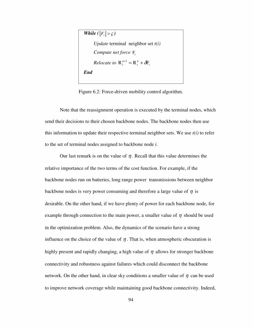
94
While ( ς>iF )
Update terminal neighbor set t(i)
Compute net force iF
Relocate to i
n
i
1n
i FRR δ+=+
End
Figure 6.2: Force-driven mobility control algorithm.
Note that the reassignment operation is executed by the terminal nodes, which
send their decisions to their chosen backbone nodes. The backbone nodes then use
this information to update their respective terminal neighbor sets. We use t(i) to refer
to the set of terminal nodes assigned to backbone node i.
Our last remark is on the value of η . Recall that this value determines the
relative importance of the two terms of the cost function. For example, if the
backbone nodes run on batteries, long range power transmissions between neighbor
backbone nodes is very power consuming and therefore a large value of η is
desirable. On the other hand, if we have plenty of power for each backbone node, for
example through connection to the main power, a smaller value of η should be used
in the optimization problem. Also, the dynamics of the scenario have a strong
influence on the choice of the value of η . That is, when atmospheric obscuration is
highly present and rapidly changing, a high value of η allows for stronger backbone
connectivity and robustness against failures which could disconnect the backbone
network. On the other hand, in clear sky conditions a smaller value of η can be used
to improve network coverage while maintaining good backbone connectivity. Indeed,

95
in either case the mathematical formulation of the cost function and our optimization
scheme is capable of modeling the problem.
6.5 Spring System
In this section we present a quadratic optimization method for coverage and
connectivity control in DWB-based networks in clear atmospheric conditions. We
show that when the effects of atmospheric obscuration can be neglected, the cost
function U for the network system is analogous to the potential energy of a spring
system where wireless links are replaced by physical springs exerting forces on
network nodes. We show that Hooke-type forces [53] can be defined at each
backbone node, which drive the network topology to achieve energy minimizing
configurations.
6.5.1 Quadratic optimization
In clear atmospheric conditions we can neglect the effects of atmospheric
obscuration ( 0=ijα ) and assume a path loss exponent of n = 2. Then the link cost uij
becomes:
2
0
4L
k
ADPu
ij
j
eR
i
T
j
Rij
43421
π= , (6.23)
which is a quadratic function of L, the link distance. The link margin PR0 is
determined by the receiver sensitivity and the turbulence induced fading as defined in

96
section 4.2.2. Initially, we assume the deployment area of the backbone nodes to
share the same turbulence conditions and thus PR0 will not change with the location of
the backbone nodes. The eRT AD
π4 constant will also be independent of the backbone
nodes’ locations and will be determined by the directivity of the transmitter antenna
DT and the effective receiver area AeR . Thus, we can reformulate the link cost
function as:
2
jiijij RRku −= , where j
eR
i
T
j
RijAD
Pkπ4
0= , (6.24)
which is analogous to the potential energy of a spring with spring constant ijk and
displacement ji RR − [53]. Using this link cost function (Eq. 6.24), we can model
wireless links as springs which exert attraction forces between network nodes for
energy minimization. The beauty of this model is that given the link margin PR0 and
the receiver area eRA , the spring constant is inversely proportional to the transmitter
directivity TD . Thus, directional wireless links which have high directivities translate
into springs with low spring constants, which allow for higher link distances. On the
other hand, omnidirectional wireless links use low directivity antennas associated
with high spring constants that require much more energy to elongate. This result is
very much in accordance with our network architecture, where directional wireless
links are used to connect backbone nodes over large distances, whereas
omnidirectional wireless links are used to connect each terminal node to its assigned
base station.

97
Using the spring link cost model 6.13, the mobility control problem
formulation becomes:
∈
=
=
−+
−⋅= ∑∑∑
== =
o.w. 0
if 1 and
,4
where
rRRR)R,...,R(min
0
1
2
)h()(
1
2
ji
1
N1
T(i,j)b
ADPk
kkbU
ij
j
eR
i
T
j
Rij
G
M
k
kkkkh
F
N
i
ij
N
j
ij
π
η
444 3444 214444 34444 21
(6.25)
The goal of the optimization problem is to find the locations of all the
backbone nodes that minimize the above cost function. A very interesting property of
the above cost function is that due to its quadratic form it can be solved analytically,
and the locations found by solving the optimization problem are always inside the
network, given the convexity of the feasible region. Moreover, this cost function is
analogous to the potential energy of an equivalent network with edges replaced by
springs, with spring constants as defined in Eq. 6.24. Thus, we can model the DWB
network as a spring system whose potential energy is analogous to the
communication cost of the DWB network. In a spring system, nodes move according
to the forces exerted by the springs attached to them until reaching an equilibrium
configuration where the net force on each node is equal to zero [53]. The equilibrium
configuration is also the configuration that minimizes the potential energy of the
spring system.
Note that the above cost function is not mutually convex. Thus, to increase the
confidence margin of optimality of the solution, a perturbation method is used. The
perturbation is applied several times after each time that the algorithm converges. If

98
the force-driven algorithm converges to the same solution after a certain number of
times (typically, 2-3 times) the corresponding solution is chosen as a global optimal
solution with a high degree of confidence.
In the following section, we derive the force-driven mobility control algorithm
for the spring system model.
6.5.2 SPRING algorithm
As explained in section 6.3, the value of the net force at backbone node i is
computed as the gradient of the energy function U with respect to the location the
backbone node Ri and can be described as:
∑∑==
=+=+=M
k
ikk
N
j
ij ihb1
)(ij
1
c
i
b
ii f)(1fFFF ηη (6.26)
where ijf is described using Eq. 6.15 as:
ij
RR
ji
RR
0ij RRR24
fjiji
−+
=
−− ijijee
ADP ijj
eR
j
T
j
R
ααα
π (6.27)
Note that in the case of the spring system, 0=ijα for all i, j, thus ijf becomes:
ijij0ij R2R24
f ijj
eR
j
T
j
R kAD
P =
=
π (6.28)
with ijk as described in 6.24. Note that the force ijf in 6.28 is a weighted average of
the distance vectors between backbone node i and its neighbors. This result is in
agreement with the behavior of an analogous spring system, where nodes react based

99
on forces exerted by neighbor nodes and move in the direction of the weighted
average position of its neighbors.
Note that the force on a given backbone node only depends on the location of
its neighbors. Thus, a completely distributed algorithm can be designed where each
backbone node reacts locally to the forces exerted by neighbor nodes, providing
scalability and robustness. No centralized global information is needed. Each
backbone node can make movement decisions by itself informed by purely local
information and the overall network achieves global optimal configurations.
The SPRING optimization algorithm can be derived from the general
methodology described in section 6.3, which is based on two main operations:
relocation and reassignment. Recall that the relocation operation uses the value of the
force to find the node’s new location, as:
i
n
i
1n
i FRR δ+=+ .
Using Eq. 6.9 for the net force on backbone node i, iF , the relocation
operation is described as:
=++= ∑∑
==
+M
k
ikkij
N
j
ij fihfb1
)(
1
n
i
1n
i )(1RR ηδ . (6.29)
For the spring system case, using Eq. 6.28, the above operation becomes:
=++= ∑∑
==
+M
k
ikikkijij
N
j
ij kihkb1
n
)(
n
1
n
i
1n
i R)(1R2RR ηδ (6.30)
Note that the new location found using 6.30 is one step size in the path
between the current location of node i and the weighted average of the location of its
neighbors, with weights defined by the spring constants kij.

100
The reassignment operation was also described in section 6.3 as:
Niukh ki
n ≤≤= 1for ),r,R(minarg)( i , where h(k) denotes the index of the
backbone node assigned to terminal node k. Using the expression for the link cost in
Eq. 6.24, the reassignment operation for the spring algorithm becomes:
Ni
kkh ik
n
≤≤
−=
1
rRminarg)(2
kii (6.31)
The SPRING algorithm thus follows the same form as the general force-
driven mobility control algorithm illustrated in Fig. 6.2:
For each backbone node i
While ( ς>iF )
Update terminal neighbor set t(i)
Compute net force iF
Relocate to i
n
i
1n
i FRR δ+=+
End
where now the force iF is defined by Eqs. 6.9-6.15.
6.5.3 Simulation results
In order to gain more insight on the problem and verify the performance of
our optimization algorithm, we present results from simulation studies with different
design parameters.

101
In our initial simulations, N terminal nodes are distributed in a 100x100 two
dimensional plane. Terminal nodes are organized in clusters. The first terminal node
is placed in the plane according to a uniform random distribution. Each other terminal
is placed within clusterRange of the previous terminal node with probability
p_cluster, and uniformly in the 100x100 plane with probability 1-p_cluster. Next, M
backbone nodes are placed at random in the plane and an initial ring topology is built
connecting all backbone nodes. Then, the SPRING algorithm is executed to make
backbone nodes adjust their position until convergence to the optimal backbone
configuration.
Before we report quantitative results, we first present several figures to
visually illustrate the effectiveness of the mobility control algorithm. Fig. 6.3 shows
results for a network with 100 terminal nodes and 10 backbone nodes. The values
used for the variables clusterRange and p_cluster are 10 and 0.2 respectively. The
backbone nodes are labeled and the links between them are shown in thick dotted
lines. Links from each terminal node to its closest backbone node are shown in
thinner dotted lines.
Fig. 6.3a shows the initial non-optimal network configuration. Fig. 6.3b shows
the resulting network configuration after running the mobility control algorithm with
a balancing factor 1=η . In this case, the low value of η allows backbone nodes to
move close to the terminal nodes to optimize network coverage at the expense of low
backbone connectivity. Figs. 6.3c and 6.3d show the resulting network configurations
with 5=η and 10=η respectively. The higher value of η the more weight is put on
the backbone connectivity objective thus making the backbone nodes move closer to

102
each other. Finally, Figs. 6.3e and 6.3f show the resulting network configurations for
20=η and 30=η , where stronger backbone networks are produced at the expense
of lower network coverage.
In Fig. 6.4 we show a network with 20 backbone nodes. The number of
terminals remains 100 and they are randomly placed according to the procedure
explained above. As seen in Fig. 6.4, the increased number of backbone nodes allows
more flexibility to optimize network coverage with less penalization on backbone
connectivity, and vice versa.
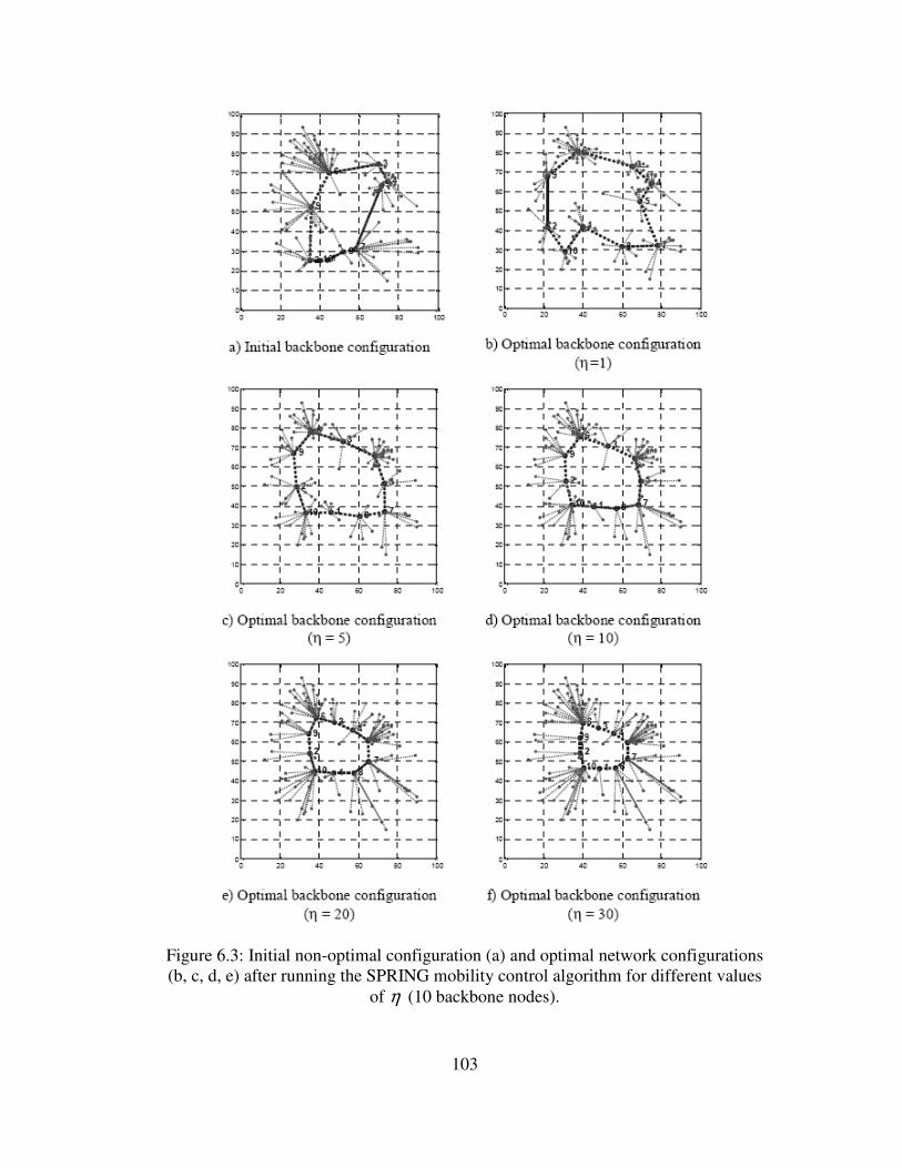
103
Figure 6.3: Initial non-optimal configuration (a) and optimal network configurations
(b, c, d, e) after running the SPRING mobility control algorithm for different values
of η (10 backbone nodes).

104
Figure 6.4: Initial non-optimal configuration (a) and optimal network configurations
(b, c, d, e) after running the SPRING mobility control algorithm for different values
of η (20 backbone nodes).

105
In order to quantitatively show the performance of our mobility control
algorithm, we computed the coverage and connectivity cost metrics for the Pareto
optimal network configurations obtained. Again, we considered networks with 100
terminal nodes and with 10 and 20 backbone nodes respectively. We used the
following set of weights: 0.01, 0.3, 1, 3, 5, 10, 15, 20, 25, and 30, to generate 10
Pareto optimal solutions for the networks under study. Fig. 6.5 shows the Pareto
optimal curves obtained. The x axis represents the coverage cost metric G, while the y
axis represents de connectivity cost metric F. We used FSO links for the backbone-to-
backbone links with 2 mrad half beam divergence and RF links for the terminal-to-
backbone links with 4/π rad half beam divergence. The minimum required received
power used was -45 dBm (31.6 nW) for all network nodes. The values of F and G
obtained were normalized and scaled for the plot in Fig. 6.5.
Since the algorithm is solving a multi-objective optimization problem, optimal
solutions, which combine low values of both cost metrics, must lie in the south-west
corner of the solution space, as shown in Fig. 6.5. Note that the increased number of
resources (base stations or backbone nodes) allows for improved Pareto optimization,
as shown by the deeper south-west configuration of the Pareto optimal curve
associated with the 20 backbone node network in the solution space. Fig. 6.5 also
shows the limit on the network coverage cost metric. As we lower the weight on
backbone connectivity, the network coverage cost decreases until reaching a point
where no further improvement is possible for the given number of backbone nodes.
As expected, when using 20 backbone nodes, network coverage can be further
optimized due to the increased number of resources. The backbone connectivity cost

106
metric, on the other hand, can be brought to zero by increasing the balancing factor
η , which would lead to a network configuration where all backbone nodes converge
into a single point. As seen in Fig. 6.5, both curves tend to zero as the weight on
backbone connectivity is increased.
Figure 6.5: Pareto Optimal set of solutions (10 and 20 backbone nodes).
In order to show the self-organizing capability of our network system, we
developed a simulation environment that outputs video sequences of dynamic
network scenarios. The objective is to show that our self-organized network system is
able to track the network dynamics.

107
As explained in Chapter 3, uncontrollable parameters such as the mobility of
the terminal nodes and the atmospheric conditions constitute the network dynamics,
which are modeled as external excitations to the network system. In this section, we
assume clear atmospheric conditions and thus the scenario dynamics is based on the
mobility of the terminal nodes. We first place N terminal nodes organized in clusters
in a two dimensional plane following the procedure introduced earlier in this section.
We then use the Reference Point Group Mobility (RPGM) model [54] to move the
terminal clusters in the plane and show how the backbone system is able to react to
the mobility of the terminal nodes driven by local forces that minimize the energy of
the network system.
First, in Fig. 6.6, we show a sequence of snapshots of the evolution of the
network form an initial non-optimal configuration to the optimal configuration driven
by local forces computed using the SPRING algorithm. In 6.6a we show the initial
placement of the terminal nodes. In this case, 100 terminal nodes are placed in a
50km x 50km plane. These terminal nodes constitute the demand for broadband
connectivity. For that purpose, a “squat team” of backbone nodes are dropped in the
area in order to form a backbone network to interconnect the terminal nodes. Fig.
6.6b shows the initial placement of the backbone nodes. The backbone nodes are
deployed at an altitude of 0.5km. Fig. 6.6 shows 2D projections of the 3D scenario.
Next, in Fig. 6.6c the backbone nodes form an initial backbone topology. We use ring
topologies to assure resilience through bi-connectivity (as explained in Chapter 5).
Fig. 6.6d shows the result of the initial reassignment step and the computation of the
forces that arise at each backbone node. The green solid lines at each backbone node
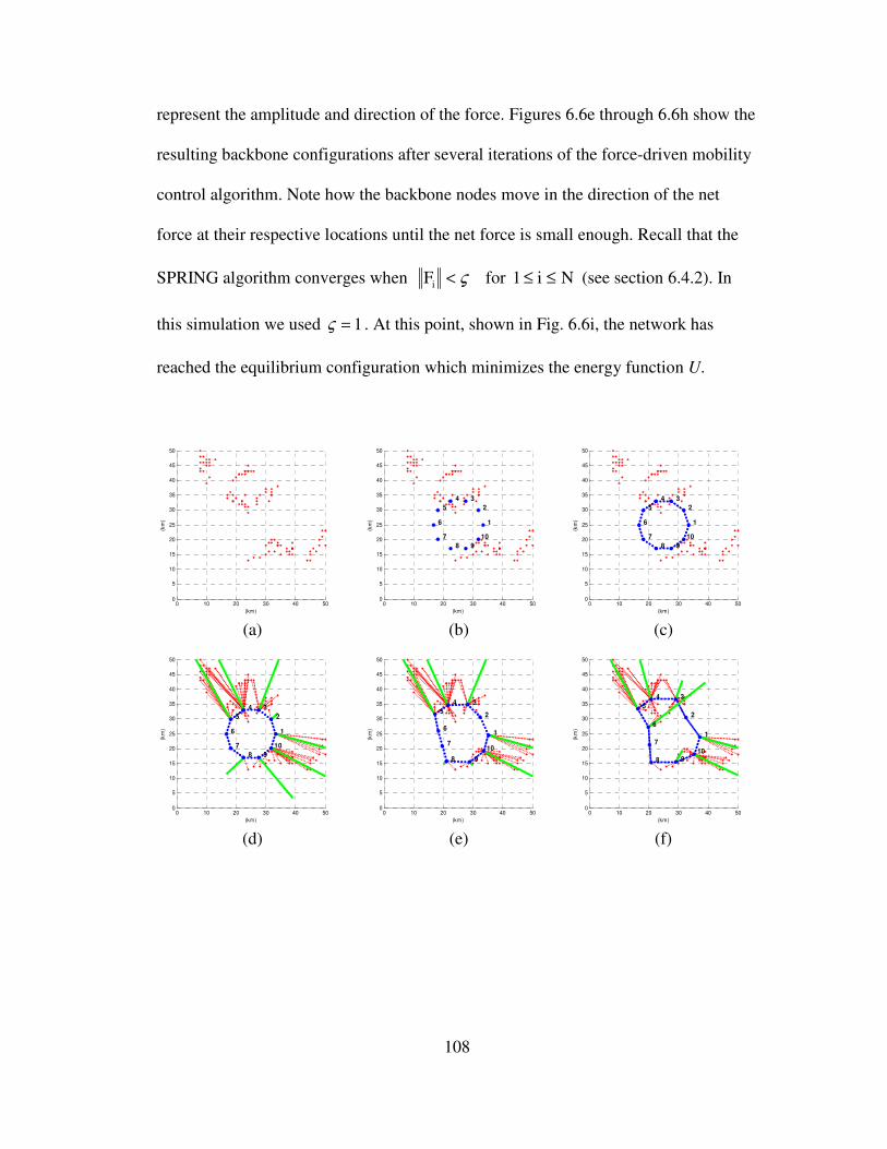
108
represent the amplitude and direction of the force. Figures 6.6e through 6.6h show the
resulting backbone configurations after several iterations of the force-driven mobility
control algorithm. Note how the backbone nodes move in the direction of the net
force at their respective locations until the net force is small enough. Recall that the
SPRING algorithm converges when Ni1for Fi ≤≤< ς (see section 6.4.2). In
this simulation we used 1=ς . At this point, shown in Fig. 6.6i, the network has
reached the equilibrium configuration which minimizes the energy function U.
0 10 20 30 40 500
5
10
15
20
25
30
35
40
45
50
(km)
(km
)
(a)
0 10 20 30 40 500
5
10
15
20
25
30
35
40
45
50
(km)
(km
) 1
2
3 4
5
6
7
8 9
10
(b)
0 10 20 30 40 500
5
10
15
20
25
30
35
40
45
50
(km)
(km
) 1
2
3 4
5
6
7
8 9
10
(c)
0 10 20 30 40 500
5
10
15
20
25
30
35
40
45
50
(km)
(km
) 1
2
3 4
5
6
7
8 9
10
(d)
0 10 20 30 40 500
5
10
15
20
25
30
35
40
45
50
(km)
(km
)
1
2
3 4
5
6
7
8 9
10
(e)
0 10 20 30 40 500
5
10
15
20
25
30
35
40
45
50
(km)
(km
)
1
2
3 4
5
6
7
8 910
(f)

109
0 10 20 30 40 500
5
10
15
20
25
30
35
40
45
50
(km)
(km
)
1
2
3 4
5
6
7
8 9 10
(g)
0 10 20 30 40 500
5
10
15
20
25
30
35
40
45
50
(km)
(km
)
1
2
3
4
5
6
7
8
9 10
(h)
0 10 20 30 40 500
5
10
15
20
25
30
35
40
45
50
(km)
(km
)
1
2
3
4
5
6
7
8
910
(i)
0 10 20 30 40 500
5
10
15
20
25
30
35
40
45
50
(km)
(km
)
1
2
3
4 5
6
7
8
910
(j)
0 10 20 30 40 500
5
10
15
20
25
30
35
40
45
50
(km)
(km
)
1
2
3
4 5
6
7
8
910
(k)
0 10 20 30 40 500
5
10
15
20
25
30
35
40
45
50
(km)
(km
)
1
2
3
4
5
6
7
8
910
(l)
Figure 6.6: Network evolution from initial placement to equilibrium for a fixed
terminal nodes’ position scenario.
In Fig. 6.7 we show a sequence of snapshots of a simulation where terminal
nodes move based on the RPGM model. Figs. 6.7a-6.7c show the evolution of the
backbone network until the equilibrium configuration for the initial placement of the
network nodes. Note that in Fig. 6.7 we also show the 3D view of the network (upper
left corner), the evolution of the energy function U, as well as the energy cost
functions for coverage (G) and connectivity (F) (lower left corner), and the amplitude
of the forces at each backbone node (lower right corner). With these four plots in each
figure, we can obtain a really good understanding of the network dynamics and the
system’s self-organizing capability. In this simulation we again used FSO links for
the backbone-to-backbone links with 2 mrad half beam divergence and RF links for

110
the terminal-to-backbone links with 4/π rad half beam divergence. The minimum
required received power used was also -45 dBm (31.6 nW) for all network nodes.
As it can be observed in Fig. 6.7a, the initial non-optimal configuration is
characterized by a high potential energy value U = 5557.24W. This energy cost is
mainly due the coverage cost G = 5557.22W. The backbone connectivity cost is fairly
small (F = 0.02W) since the backbone nodes are initially placed close to each other.
Note that the amplitudes of the forces are very large indicating the need for a
topology adjustment in order to minimize the energy of the system. Fig. 6.7b shows
the resulting network configuration after 1.5 minutes of backbone reaction using the
SPRING algorithm (the velocity of the backbone nodes used is 4 km/min). Note how
the backbone topology has stretched driven by the forces acting at each backbone
node and the total energy of the system has dropped to U = 2012.7W. The coverage
cost has also reduced to G = 2012.6W and the connectivity cost (F = 0.10W) has
slightly increased due to the increased distances between backbone nodes. Fig. 6.7c
shows the optimal configuration obtained after the equilibrium condition is met. The
amplitudes of the forces are now Ni1for 1Fi ≤≤< and the energy of the system
has reduced to U = 372.57W. In this case, the network took 5 minutes to converge to
the optimal configuration from the initial placement shown in Fig. 6.7a.
After this point the RPGM model is used to move the terminal nodes. The
velocity of the terminals is chosen to be 2 km/min and the location of the terminal
nodes is updated every 1 minute. Fig. 6.7d shows the new state of excitation of the
network system caused by the first update on the mobility of the terminal nodes. Note
that as soon as the update is received, a new reassignment operation is executed and

111
new forces appear at each backbone node. The energy of the system has increased to
U = 424.89W and new forces arise to make the network react to the external
excitation. Thus in this simulation (Fig. 6.7), the excitation caused by the terminal
nodes mobility is illustrated in the following ways:
1) The total energy of the system U increases.
2) The coverage energy cost increases: this is due to the additional energy
needed to communicate with terminal nodes that have moved out of their
optimal positions with respect to the backbone network.
3) The connectivity energy cost remains constant. The backbone nodes have
yet to move and thus this cost function does not change.
4) New forces appear at the backbone nodes as a result of the excitation to
the network system.
Fig. 6.7e shows the resulting configuration after 0.5 minutes of reaction. Note
how in Fig. 6.7e, after 0.5 minutes of reaction, the network has converged to an
optimal configuration where the total energy U has decreased from 424.89W to
369.04W and the amplitudes of the net forces acting on each backbone node are close
to zero.
Fig. 6.7f shows a new excitation to the network system caused by the
terminals’ mobility. The total energy of the system goes up to 503.51W and new
forces arise at each backbone node that make the network adjust its topology. Figs.
6.7g and 6.7h show two snapshots of the backbone reaction after 0.5 and 1 minute
respectively. In this case, the network is able to reduce the energy to U = 409.70W,
but does not reach equilibrium before a new update is received (Fig. 6.7i).

112
Note how in the rest of the sequence (Figs. 6.7j-6.7t) the network is able to
continue reacting to the excitations by following the local forces computed at each
backbone node.
1 2 3 4 5 6 7 8 9 100
50
100
150
200
Backbone Node ID
Fo
rce
(k
m)
Total Cost Coverage Cost Connectivity Cost0
2000
4000
6000
8000
10000
Co
st
(Wa
tts
)
0 10 20 30 40 500
5
10
15
20
25
30
35
40
45
50
(km)
(km
) 1
2 3 4
5
6
7 8 9
10
010
2030
4050
0
10
20
30
40
50
00.51
(km)
10 1
9
2
8
3
7
4
6 5
(km)
(km
)
(a) Initial placement (0 min):
U = 5557.24W; G = 5557.22W; F = 0.02W

113
1 2 3 4 5 6 7 8 9 100
50
100
150
200
Backbone Node IDF
orc
e (
km
)
Total Cost Coverage Cost Connectivity Cost0
1000
2000
3000
4000
Co
st
(Wa
tts)
0 10 20 30 40 500
5
10
15
20
25
30
35
40
45
50
(km)
(km
)
1
2
3
4
5
6
7
8
910
010
2030
4050
0
10
20
30
40
50
00.51
10
1
(km)
2
8
9
3
7
4
6
5
(km)
(km
)
(b) Backbone reaction (1.5 min):
U = 2012.7W; G = 2012.6W; F = 0.10W
1 2 3 4 5 6 7 8 9 100
50
100
150
200
Backbone Node ID
Fo
rce
(k
m)
Total Cost Coverage Cost Connectivity Cost0
100
200
300
400
500
600
700
Co
st
(Wa
tts)
0 10 20 30 40 500
5
10
15
20
25
30
35
40
45
50
(km)
(km
)
1
2
3
4
5
6
7 8
9
10
010
2030
4050
0
10
20
30
40
50
00.51 1
10
(km)
2
8
9
3
4
7
6
5
(km)
(km
)
(c) Backbone reaction (5 min):
Equilibrium: U = 372.57W; G = 372.42W; F = 0.15W

114
1 2 3 4 5 6 7 8 9 100
50
100
150
200
Backbone Node IDF
orc
e (
km
)
Total Cost Coverage Cost Connectivity Cost0
200
400
600
800
Co
st
(Wa
tts)
0 10 20 30 40 500
5
10
15
20
25
30
35
40
45
50
(km)
(km
)
1
2
3
4
5
6
7 8
9
10
010
2030
4050
0
10
20
30
40
50
00.51 1
10
(km)
2
8
9
3
4
7
6
5
(km)
(km
)
(d) Terminals location update (5 min):
U = 424.89W; G = 424.74W; F = 0.15W
1 2 3 4 5 6 7 8 9 100
50
100
150
200
Backbone Node ID
Fo
rce
(k
m)
Total Cost Coverage Cost Connectivity Cost0
100
200
300
400
500
600
700
Co
st
(Wa
tts)
0 10 20 30 40 500
5
10
15
20
25
30
35
40
45
50
(km)
(km
)
1
2
3
4
5
6
7 8
9
10
010
2030
4050
0
10
20
30
40
50
00.51
10
1
(km)
2
9
8
3
4
7
6
5
(km)
(km
)
(e) Backbone reaction (5.5 min):
Equilibrium: U = 369.04W; G = 368.91W; F = 0.13W
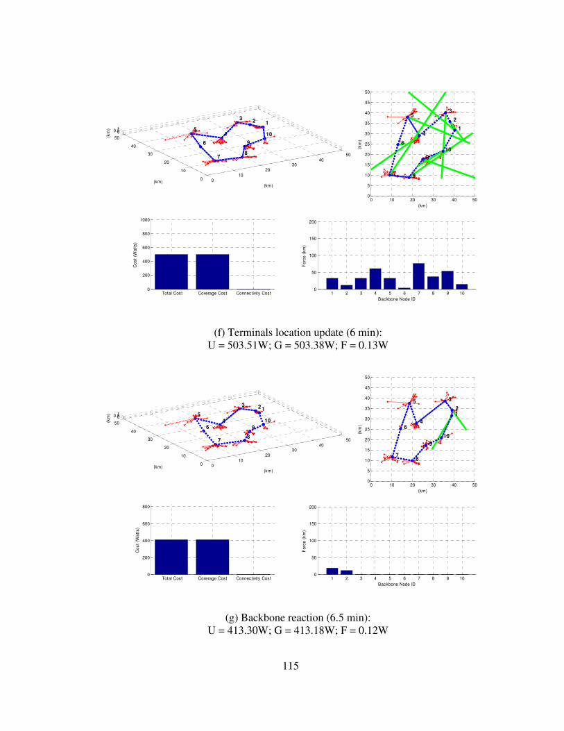
115
1 2 3 4 5 6 7 8 9 100
50
100
150
200
Backbone Node IDF
orc
e (
km
)
Total Cost Coverage Cost Connectivity Cost0
200
400
600
800
1000
Co
st
(Wa
tts)
0 10 20 30 40 500
5
10
15
20
25
30
35
40
45
50
(km)
(km
)
1
2
3
4
5
6
7 8
9
10
010
2030
4050
0
10
20
30
40
50
00.51
10
1
(km)
2
9
8
3
4
7
6
5
(km)
(km
)
(f) Terminals location update (6 min):
U = 503.51W; G = 503.38W; F = 0.13W
1 2 3 4 5 6 7 8 9 100
50
100
150
200
Backbone Node ID
Fo
rce
(k
m)
Total Cost Coverage Cost Connectivity Cost0
200
400
600
800
Co
st
(Wa
tts)
0 10 20 30 40 500
5
10
15
20
25
30
35
40
45
50
(km)
(km
)
1 2
3
4
5
6
7 8
9
10
010
2030
4050
0
10
20
30
40
50
00.51
10
(km)
1 2
9
8
3
4
7
6
5
(km)
(km
)
(g) Backbone reaction (6.5 min):
U = 413.30W; G = 413.18W; F = 0.12W

116
1 2 3 4 5 6 7 8 9 100
50
100
150
200
Backbone Node IDF
orc
e (
km
)
Total Cost Coverage Cost Connectivity Cost0
200
400
600
800
Co
st
(Wa
tts)
0 10 20 30 40 500
5
10
15
20
25
30
35
40
45
50
(km)
(km
)
1
2
3
4
5
6
7 8
9
10
010
2030
4050
0
10
20
30
40
50
00.51
10
(km)
1 2
9
8
3
4
7
6
5
(km)
(km
)
(h) Backbone reaction (7 min):
U = 409.70W; G = 409.58; F = 0.12W
1 2 3 4 5 6 7 8 9 100
50
100
150
200
Backbone Node ID
Fo
rce
(k
m)
Total Cost Coverage Cost Connectivity Cost0
200
400
600
800
1000
Co
st
(Wa
tts)
0 10 20 30 40 500
5
10
15
20
25
30
35
40
45
50
(km)
(km
)
1
2
3
4
5
6
7 8
9
10
010
2030
4050
0
10
20
30
40
50
00.51
10
(km)
1 2
9
8
3
4
7
6
5
(km)
(km
)
(i) Terminals location update (7 min):
U = 591.81W; G = 591.69W; F = 0.12W

117
1 2 3 4 5 6 7 8 9 100
50
100
150
200
Backbone Node IDF
orc
e (
km
)
Total Cost Coverage Cost Connectivity Cost0
200
400
600
800
Co
st
(Wa
tts)
0 10 20 30 40 500
5
10
15
20
25
30
35
40
45
50
(km)
(km
)
1
2 3
4
5
6
7 8
910
010
2030
4050
0
10
20
30
40
50
00.51
(km)
10
1
9
2
8
3
4
7
6
5
(km)
(km
)
(j) Backbone reaction (7.5 min):
U = 429.84W; G = 429.73W; F = 0.11W
1 2 3 4 5 6 7 8 9 100
50
100
150
200
Backbone Node ID
Fo
rce
(k
m)
Total Cost Coverage Cost Connectivity Cost0
200
400
600
800
Co
st
(Wa
tts)
0 10 20 30 40 500
5
10
15
20
25
30
35
40
45
50
(km)
(km
) 1
2 3
4
5
6
7 8
910
010
2030
4050
0
10
20
30
40
50
00.51
(km)
10
1
9
2
8
3
4
7
6
5
(km)
(km
)
(k) Backbone reaction (8 min):
Equilibrium: U = 432.83W; G = 432.72W; F = 0.11W

118
1 2 3 4 5 6 7 8 9 100
50
100
150
200
Backbone Node IDF
orc
e (
km
)
Total Cost Coverage Cost Connectivity Cost0
200
400
600
800
1000
Co
st
(Wa
tts)
0 10 20 30 40 500
5
10
15
20
25
30
35
40
45
50
(km)
(km
) 1
2 3
4
5
6
7 8
910
010
2030
4050
0
10
20
30
40
50
00.51
(km)
10
1
9
2
8
3
4
7
6
5
(km)
(km
)
(l) Terminals location update (8 min):
U = 598.54W; G = 598.43W; F = 0.11W
1 2 3 4 5 6 7 8 9 100
50
100
150
200
Backbone Node ID
Fo
rce
(k
m)
Total Cost Coverage Cost Connectivity Cost0
200
400
600
800
1000
Co
st
(Wa
tts)
0 10 20 30 40 500
5
10
15
20
25
30
35
40
45
50
(km)
(km
)
1
2 3
4
5
6
7 8
9
10
010
2030
4050
0
10
20
30
40
50
00.51
(km)
910
1
8
2 3
4
7
6
5
(km)
(km
)
(m) Backbone reaction (8.5 min):
U = 502.12W G = 502.03W; F = 0.09W

119
1 2 3 4 5 6 7 8 9 100
50
100
150
200
Backbone Node IDF
orc
e (
km
)
Total Cost Coverage Cost Connectivity Cost0
200
400
600
800
Co
st
(Wa
tts)
0 10 20 30 40 500
5
10
15
20
25
30
35
40
45
50
(km)
(km
)
1
2 3
4
5
6
7 8
9
10
010
2030
4050
0
10
20
30
40
50
00.51
(km)
910
1
8
2 3
4
7
6
5
(km)
(km
)
(n) Backbone reaction (9 min):
U = 487.78W; G = 487.69W; F = 0.09W
1 2 3 4 5 6 7 8 9 100
50
100
150
200
Backbone Node ID
Fo
rce
(k
m)
Total Cost Coverage Cost Connectivity Cost0
200
400
600
800
1000
1200
Co
st
(Wa
tts)
0 10 20 30 40 500
5
10
15
20
25
30
35
40
45
50
(km)
(km
)
1
2 3
4
5
6
7 8
9
10
010
2030
4050
0
10
20
30
40
50
00.51
(km)
910
1
8
2 3
4
7
6
5
(km)
(km
)
(o) Terminals location update (9 min):
U = 665.31W; G = 665.22W; F = 0.09W

120
1 2 3 4 5 6 7 8 9 100
50
100
150
200
Backbone Node IDF
orc
e (
km
)
Total Cost Coverage Cost Connectivity Cost0
200
400
600
800
Co
st
(Wa
tts)
0 10 20 30 40 500
5
10
15
20
25
30
35
40
45
50
(km)
(km
)
1
2 3
4
5
6
7 8 9
10
010
2030
4050
0
10
20
30
40
50
00.51
9
(km)
10
1
8
2 3
7
4
6
5
(km)
(km
)
(p) Backbone reaction (9.5 min):
U = 461.73W; G = 461.66W; F = 0.07W
1 2 3 4 5 6 7 8 9 100
50
100
150
200
Backbone Node ID
Fo
rce
(k
m)
Total Cost Coverage Cost Connectivity Cost0
100
200
300
400
500
600
700
Co
st
(Wa
tts)
0 10 20 30 40 500
5
10
15
20
25
30
35
40
45
50
(km)
(km
)
1
2 3
4 5
6
7 8 9
10
010
2030
4050
0
10
20
30
40
50
00.51
9
(km)
10
1 2
8
3
7
4
6
5
(km)
(km
)
(q) Backbone reaction (10 min):
U = 374.67W; G = 374.60W; F = 0.07W

121
1 2 3 4 5 6 7 8 9 100
50
100
150
200
Backbone Node IDF
orc
e (
km
)
Total Cost Coverage Cost Connectivity Cost0
200
400
600
800
Co
st
(Wa
tts)
0 10 20 30 40 500
5
10
15
20
25
30
35
40
45
50
(km)
(km
)
1
2 3
4 5
6
7 8 9
10
010
2030
4050
0
10
20
30
40
50
00.51
9
(km)
10
1 2
8
3
7
4
6
5
(km)
(km
)
(r) Terminals location update (10 min):
U = 459.90W; G = 459.83W; F = 0.07W
1 2 3 4 5 6 7 8 9 100
50
100
150
200
Backbone Node ID
Fo
rce
(k
m)
Total Cost Coverage Cost Connectivity Cost0
100
200
300
400
500
600
700
Co
st
(Wa
tts)
0 10 20 30 40 500
5
10
15
20
25
30
35
40
45
50
(km)
(km
)
1
2 3
4 5
6
7 8
9
10
010
2030
4050
0
10
20
30
40
50
00.51
9
(km)
10
1
8
2 3
7
4
6
5
(km)
(km
)
(s) Backbone reaction (10.5 min):
U = 350.71W; G = 350.65W; F = 0.06W

122
1 2 3 4 5 6 7 8 9 100
50
100
150
200
Backbone Node IDF
orc
e (
km
)
Total Cost Coverage Cost Connectivity Cost0
100
200
300
400
500
600
Co
st
(Wa
tts)
0 10 20 30 40 500
5
10
15
20
25
30
35
40
45
50
(km)
(km
)
1
2 3
4 5
6
7 8
9
10
010
2030
4050
0
10
20
30
40
50
00.51
9
(km)
10
1
8
2 3
7
4
6
5
(km)
(km
)
(t) Backbone reaction (11 min):
U = 336.79W; G = 336.72W; F = 0.07W
Figure 6.7: Network evolution with terminal clusters moving according to the RPGM
model and backbone reacting using the SPRING algorithm.
In order to show the performance of the SPRING algorithm, we compared the
average energy per unit time used in networks using the SPRING mobility control
algorithm, with respect to: 1) networks with the base stations fixed at the initial
optimal configuration and 2) networks using and average algorithm where the base
stations move to he average position of its neighbors. We executed simulations for 10
and 20 backbone node networks, and for 10 different 1 hour scenario patterns
(involving different terminal node placement and mobility patterns).
Table 6.1 shows the results obtained. As expected, when using fixed base
stations, high energy values are needed to maintain network performance. The

123
continuous excitation produced by the network dynamics (terminal nodes’ mobility)
is not balanced due to the lack of a self-organizing capability.
One intuitive way of moving backbone nodes is to move them in the direction
of the average position of its neighbors. We will refer to this method as the AVG
algorithm. As seen in section 6.5, the solution to the energy minimization problem for
the SPRING system makes nodes move in the direction of the weighted average of
their neighbor’s positions with weights defined based on the wireless technologies
used. Thus, the AVG algorithm is an instance of the SPRING algorithm in the case of
a homogeneous network architecture, where all communication nodes have the same
communication capabilities. Our network scenarios are characterized by a
heterogeneous architecture and thus the SPRING algorithm is able to outperform the
AVG algorithm by taking into account the different behavior of wireless links using
different communication technologies. Recall that in this simulation the backbone-to-
backbone links are FSO links with mrad 2=θ and the terminal-to-backbone links
are RF links with rad 4/πθ = . The SPRING algorithm is able to minimize the
energy of the network system by driving the network topology in the direction of the
steepest decrease of the global energy function. Note from table 6.1 that the SPRING
algorithm uses on average 41% less energy than the AVG algorithm when using 10
backbone nodes, and a 58% reduction is obtained for 20 backbone nodes networks.
10 backbone
nodes
20 backbone
nodes
No mobility control 2391 W 1750 W

124
AVG algorithm 543 W 249 W
SPRING algorithm 318 W 104 W
Percentage improvement
(SPRING v.s. No mobility) 87 % 94 %
Percentage improvement
(SPRING v.s. AVG) 41 % 58 %
Table 6.1: Average percentage improvement in total average power usage using the
SPRING mobility control algorithm versus using the AVG algorithm and versus no
mobility control, for networks with 10 and 20 backbone nodes.
6.6 Mobility control under atmospheric obscuration
As it has been shown throughout this dissertation, mobility control strategies
modeled as energy minimization problems strongly depend on the link cost models
used. As seen in the previous section, when no atmospheric obscuration effects are
taken into account the energy function to be minimized mimics the potential energy
of a spring system. If we introduce the effects of atmospheric obscuration, then the
link cost model becomes that of Eq. 4.8:
( )
−
=
− 2
ji
RR
0 RR4ji
j
eR
j
T
j
RijAD
ePuij πα
.
If the obscuration factor α is assumed to be constant in the area where the
backbone nodes are distributed, then the link cost becomes a function of the type

125
xekxf α2= , where x is the link length ji RR −=L . This type of function, although
not quadratic, is still convex and an exponential function of the link distance.
In this section we use our general force-driven mobility control methodology
described in section 6.2 to derive the solution to the mobility control problem in the
presence of atmospheric obscuration.
6.6.1 Convex optimization
In this section we extend our link energy model to include the effects of
atmospheric attenuation. Eq. 4.8 can be restated as follows:
ji RR2
ji RR−
−= ijeku ijij
α, (6.32)
which is the product of a quadratic function and an exponential function of the link
distance ji RR −=L . The constant kij was defined in Eq. 6.24 as j
eR
i
T
j
RijAD
Pkπ4
0= .
This link cost function in Eq. 6.32 is thus defined in terms of two main components:
1) 2
ji RR −ijk : this component models the energy needed to overcome the
effects of the free space path loss, as described in section 4.4.1. This is quadratic
function of the link distance analogous to the potential energy of a spring with spring
constant defined by the link directivity (refer to section 4.4.1).
2) ji RR −ije
α: this component models the energy needed to overcome the
effects of atmospheric attenuation, as described in section 4.4.2. This is an
exponential function of the link distance which models the scattering of
electromagnetic radiation through the atmosphere in the presence of clouds and fog

126
(refer to section 4.4.2). Note that in clear atmospheric conditions, when the scattering
coefficient α is small enough, this component can be neglected and the link cost
function becomes that of a spring system. As α increases due to the presence of
cloud layers in the atmosphere, this component imposes an exponential increase on
the energy needed to maintain the specified link BER.
Using the link energy model in Eq. 6.32, the potential energy function for the
network system becomes:
444444 3444444 2144444 344444 21G
M
k
kkh
F
N
i
ij
N
j
ij
kkhijekekbU
−+
−⋅= ∑∑∑
=
−
=
−
= 1
rR2
kh(k))(
1
RR2
ji
1
N1
kh(k))(ji rRRR)R,...,R(αα
η
. (6.33)
And thus the mobility control problem formulation is stated as follows:
∈
=
=
−
+
−⋅=
∑
∑∑
=
−
=
−
=
o.w. 0
if 1 and
,4
where
rR
RR)R,...,R(
min
0
1
rR2
kh(k))(
1
RR2
ji
1
N1
kh(k)
ji
T(i,j)b
ADPk
ek
ekbU
ij
j
eR
i
T
j
Rij
G
M
k
kkh
F
N
i
ij
N
j
ij
ij
ij
π
η
α
α
44444 344444 21
44444 344444 21
(6.34)
Again, the goal of the optimization problem is to find the locations of all the
backbone nodes that minimize the above cost function. In this case the energy
function U is not quadratic, but it is still continuous and convex.
In the following section we derive the force-driven mobility control algorithm
for network systems under atmospheric obscuration.

127
6.6.2 FORCE algorithm
Recall that in our force-driven mobility control methodology, the value of the
net force at backbone node i is computed as the gradient of the energy function U
with respect to the location the backbone node Ri, described in Eq. 6.9 as:
∑∑==
=+=+=M
k
k
N
j
ij ihb1
ik)(ij
1
c
i
b
ii f)(1fFFF ηη ,
where ijf is the force exerted on node i due the its interaction with node j, defined as
the negative gradient of the link energy function uij with respect to Ri, as:
∂
∂−
∂
∂−
∂
∂−
=−∇=
i
ij
i
ij
i
ij
ij
i
Z
u
Y
u
X
u
uijf .
Using Eq. 6.24 for the link energy function uij, ijf is described as:
−
−
−
−+−=
=−−
ji
ji
ji
ijij
zij
yij
xij
ZZ
YY
XX
eek
f
f
f
ijij
ji
RRRR
,
,
,
ij RR2fjiji αα
α ,
(6.35)
which in vector form becomes:
ij
RR
ji
RR
ij RRR2fjiji
−+=
−− ijijeek ijij
ααα . (6.36)
As it can be observed from Eq. 6.36, in the presence of atmospheric
obscuration, the force on a given backbone node still depends on local information
only. Thus, a completely distributed algorithm can be designed where each backbone

128
node reacts locally to the forces exerted by neighbor nodes, maintaining the
scalability and robustness of the control system.
Note that in this case the direction of the force is still given by the
displacement vector ijR , but the amplitude is a more complicated function of the link
distance as compared to the spring system scenario. In this case, an exponential
function of the link distance dictates the additional force exerted on network nodes in
areas of significant atmospheric obscuration. This extra force arises to bring backbone
nodes even closer to each other in order to overcome the signal power attenuation
caused by the scattering of electromagnetic radiation due to the presence of
atmospheric obscurants in the form of clouds or fog.
The optimization algorithm can be derived from the general methodology
described in section 6.4.2, which is based on two main operations: relocation and
reassignment. Recall that the relocation operation uses the value of the force to find
the node’s new location, as: i
n
i
1n
i FRR δ+=+ . In the presence of atmospheric
obscuration, using Eq. 6.36, the relocation operation becomes:
( )
( )
−+=+
−+
+=
∑
∑
=
−−
−−
=+
M
k
ikkiikikk
ijij
N
j
ij
iikiik
ijij
erekih
eekb
1
rRrR
)(
ij
RR
ji
RR
1n
i
1n
i
RR2)(1
RRR2
RR
kk
jiji
αα
αα
α
αη
δ . (6.37)
The reassignment operation was also described in section 6.3 as:
Niukh ki
n ≤≤= 1for ),r,R(minarg)( i , where h(k) denotes the index of the backbone
node assigned to terminal node k. Using the expression for the link cost in Eq. 6.32,
the reassignment operation for the spring algorithm becomes:

129
Ni
ekkh ik
ik
n
≤≤
−=−
1
rRminarg)( ki rR2
kii
α
(6.38)
The mobility control algorithm based on these two operations follow the same
form as in Fig. 6.2, but using the updated operations described above which take into
account the effects of atmospheric obscuration in the network. We refer to this
extended force-driven mobility control algorithm as the FORCE algorithm.
6.6.3 Simulation results
As we did in section 6.5.3 to validate the SPRING algorithm, in this section
we present simulation results to validate the performance of the FORCE algorithm.
Fig. 6.8 shows a sequence of snapshots of a dynamic network simulation. In
this first simulation the terminal nodes are not moving. The excitation to the network
system is caused by the presence of atmospheric obscuration. The obscuration pattern
is represented by and array that contains the average attenuation factor in km-1
for the
backbone FSO links, for every minute of the simulation.
In Fig. 6.8a the network is at equilibrium. Fig. 6.8b shows a first excitation to
the system caused by the presence of atmospheric obscuration. At this point, the
average atmospheric attenuation factor is 0.4 km-1
and thus forces appear that make
backbone nodes start moving closer to each other. No nodes have yet changed their
positions, but the energy of the system has increased from U = 308.88W to U =
347.07W due to the effects of atmospheric attenuation. Fig. 6.8c shows the resulting
configuration after 1 minute of reaction. The network has reached an equilibrium
configuration with a total energy value of U = 341.67W. Fig. 6.8d shows the effects

130
of the new update on the atmospheric attenuation coefficient which has increased to
0.6 km-1
. The backbone connectivity cost increases to F = 517.94W indicating the
extra energy needed at the FSO links forming the backbone network in order to
maintain connectivity. Fig. 6.8e shows the equilibrium configuration obtained after 1
minute of reaction. In the sequence 6.8f-6.8r the backbone network keeps reacting to
the increasing atmospheric attenuation coefficient by pulling its nodes closer to each
other. In Fig. 6.8q (minute 7), the attenuation coefficient increases to 1.6 km-1
and the
network is able to reach an equilibrium configuration at minute 7.5 where the total
energy of the system is U = 2369.6W (Fig. 6.8r). At minutes 8 and 9, the attenuation
coefficient remains at 1.6 km-1
and thus the network remains at the same optimal
configuration (Figs. 6.8s-6.8v). At minute 10, the attenuation coefficient starts
decreasing. Fig. 6.8w shows the resulting forces after α has dropped to 1.4 km-1
. Note
how now the forces make the backbone topology stretch back in the direction of the
terminal nodes as more energy can be used for coverage due to the reduction in
connectivity cost, caused by the lower atmospheric attenuation. The final sequence
(Figs. 6.8x-6.8dd) shows the reaction of the backbone topology as the atmospheric
attenuation decreases from 1.4 km-1
to 0 km-1
. Note how at minute 17 of the
simulation (Fig. 6.8dd), the backbone topology has converged back to the initial
optimal configuration of Fig. 6.8a.

131
1 2 3 4 5 6 7 8 9 100
50
100
150
200
Backbone Node IDF
orc
e (
km
)
Total Cost Coverage Cost Connectivity Cost0
100
200
300
400
500
600
Co
st
(Wa
tts)
0 10 20 30 40 500
5
10
15
20
25
30
35
40
45
50
(km)
(km
)
1 2
3
4
5
6
7
8
9
10
010
2030
4050
0
10
20
30
40
50
00.51
10
1
9
8
(km)
2
6
3
7
4
5
(km)
(km
)
(a) Initial placement (0 min):
Equilibrium: U = 308.88W; G = 308.73W; F = 0.15W
1 2 3 4 5 6 7 8 9 100
50
100
150
200
Backbone Node ID
Fo
rce
(k
m)
Total Cost Coverage Cost Connectivity Cost0
100
200
300
400
500
600
Co
st
(Wa
tts)
0 10 20 30 40 500
5
10
15
20
25
30
35
40
45
50
(km)
(km
)
1 2
3
4
5
6
7
8
9
10
010
2030
4050
0
10
20
30
40
50
00.51
10
1
9
8
(km)
2
6
3
7
4
5
(km)
(km
)
(b) Atmospheric attenuation update (α = 0.4 km
-1) (1 min):
U = 347.07W; G = 308.73W; F = 38.34W

132
1 2 3 4 5 6 7 8 9 100
50
100
150
200
Backbone Node IDF
orc
e (
km
)
Total Cost Coverage Cost Connectivity Cost0
100
200
300
400
500
600
Co
st
(Wa
tts)
0 10 20 30 40 500
5
10
15
20
25
30
35
40
45
50
(km)
(km
)
1 2
3
4
5
6
7
8
9
10
010
2030
4050
0
10
20
30
40
50
00.51
10
1
9
8
(km)
2
6
3
7
4
5
(km)
(km
)
(c) Backbone reaction (1.5 min):
Equilibrium: U = 341.67W; G = 310.38W; F = 31.29W
1 2 3 4 5 6 7 8 9 100
50
100
150
200
Backbone Node ID
Fo
rce
(k
m)
Total Cost Coverage Cost Connectivity Cost0
500
1000
1500
Co
st
(Wa
tts)
0 10 20 30 40 500
5
10
15
20
25
30
35
40
45
50
(km)
(km
)
1 2
3
4
5
6
7
8
9
10
010
2030
4050
0
10
20
30
40
50
00.51
10
1
9
8
(km)
2
6
3
7
4
5
(km)
(km
)
(d) Atmospheric attenuation update (α = 0.6 km
-1) (2 min):
U = 828.36W; G = 310.41W; F = 517.94W

133
1 2 3 4 5 6 7 8 9 100
50
100
150
200
Backbone Node IDF
orc
e (
km
)
Total Cost Coverage Cost Connectivity Cost0
200
400
600
800
1000
Co
st
(Wa
tts)
0 10 20 30 40 500
5
10
15
20
25
30
35
40
45
50
(km)
(km
)
1
2
3
4
5
6 7
8
9
10
010
2030
4050
0
10
20
30
40
50
00.51
10
1
9
8
(km)
2
6
3
7
4
5
(km)
(km
)
(e) Backbone reaction (2.5 min):
Equilibrium: U = 503.50W; G = 361.22W; F = 142.28W
1 2 3 4 5 6 7 8 9 100
50
100
150
200
Backbone Node ID
Fo
rce
(k
m)
Total Cost Coverage Cost Connectivity Cost0
1000
2000
3000
4000
Co
st
(Wa
tts)
0 10 20 30 40 500
5
10
15
20
25
30
35
40
45
50
(km)
(km
)
1
2
3
4
5
6 7
8
9
10
010
2030
4050
0
10
20
30
40
50
00.51
10
1
9
8
(km)
2
6
3
7
4
5
(km)
(km
)
(f) Atmospheric attenuation update (α = 0.8 km
-1) (3 min):
U = 2034.7W; G = 361.4W; F = 673.3W

134
1 2 3 4 5 6 7 8 9 100
50
100
150
200
Backbone Node IDF
orc
e (
km
)
Total Cost Coverage Cost Connectivity Cost0
500
1000
1500
Co
st
(Wa
tts)
0 10 20 30 40 500
5
10
15
20
25
30
35
40
45
50
(km)
(km
)
1
2
3
4
5
6 7
8
9
10
010
2030
4050
0
10
20
30
40
50
00.51
10
1
9
8
(km)
2
6
3
7
4
5
(km)
(km
)
(g) Backbone reaction (3.5 min):
U = 800.4W; G = 523.8W; F = 276.6W
1 2 3 4 5 6 7 8 9 100
50
100
150
200
Backbone Node ID
Fo
rce
(k
m)
Total Cost Coverage Cost Connectivity Cost0
500
1000
1500
Co
st
(Wa
tts)
0 10 20 30 40 500
5
10
15
20
25
30
35
40
45
50
(km)
(km
)
1
2
3
4
5
6 7
8
9
10
010
2030
4050
0
10
20
30
40
50
00.51
10
1
9
8
(km)
2
6
3
7
4
5
(km)
(km
)
(h) Backbone reaction (4 min):
Equilibrium: U = 796.6W; G = 526.7W; F = 269.9W

135
1 2 3 4 5 6 7 8 9 100
50
100
150
200
Backbone Node IDF
orc
e (
km
)
Total Cost Coverage Cost Connectivity Cost0
1000
2000
3000
4000
5000
Co
st
(Wa
tts)
0 10 20 30 40 500
5
10
15
20
25
30
35
40
45
50
(km)
(km
)
1
2
3
4
5
6 7
8
9
10
010
2030
4050
0
10
20
30
40
50
00.51
10
1
9
8
(km)
2
6
3
7
4
5
(km)
(km
)
(i) Atmospheric attenuation update (α = 1.0 km
-1) (4 min):
U = 2637.6W; G = 527.1W; F = 2110.5W
1 2 3 4 5 6 7 8 9 100
50
100
150
200
Backbone Node ID
Fo
rce
(k
m)
Total Cost Coverage Cost Connectivity Cost0
500
1000
1500
2000
Co
st
(Wa
tts)
0 10 20 30 40 500
5
10
15
20
25
30
35
40
45
50
(km)
(km
)
1
2
3 4
5
6 7
8
9
10
010
2030
4050
0
10
20
30
40
50
00.51
10
1
9
8
(km)
2
6
3
7
4
5
(km)
(km
)
(j) Backbone reaction (4.5 min):
U = 1176.1W; G = 773.1W; F = 403.0W

136
1 2 3 4 5 6 7 8 9 100
50
100
150
200
Backbone Node IDF
orc
e (
km
)
Total Cost Coverage Cost Connectivity Cost0
500
1000
1500
2000
Co
st
(Wa
tts)
0 10 20 30 40 500
5
10
15
20
25
30
35
40
45
50
(km)
(km
)
1
2
3 4
5
6 7
8
9
10
010
2030
4050
0
10
20
30
40
50
00.51
10
1
9
8
(km)
2
6
3
7
4
5
(km)
(km
)
(k) Backbone reaction (5 min):
Equilibrium: U = 1168.8W; G = 778.4W; F = 390.4W
1 2 3 4 5 6 7 8 9 100
50
100
150
200
Backbone Node ID
Fo
rce
(k
m)
Total Cost Coverage Cost Connectivity Cost0
1000
2000
3000
4000
5000
6000
Co
st
(Wa
tts)
0 10 20 30 40 500
5
10
15
20
25
30
35
40
45
50
(km)
(km
)
1
2
3 4
5
6 7
8
9
10
010
2030
4050
0
10
20
30
40
50
00.51
10
1
9
8
(km)
2
6
3
7
4
5
(km)
(km
)
(l) Atmospheric attenuation update (α = 1.2 km
-1) (5 min):
U = 3040.0W; G = 778.9W; F = 2261.1W

137
1 2 3 4 5 6 7 8 9 100
50
100
150
200
Backbone Node IDF
orc
e (
km
)
Total Cost Coverage Cost Connectivity Cost0
500
1000
1500
2000
2500
3000
Co
st
(Wa
tts)
0 10 20 30 40 500
5
10
15
20
25
30
35
40
45
50
(km)
(km
)
1
2
3 4
5
6
7
8
9
10
010
2030
4050
0
10
20
30
40
50
00.51
10 9
1
8
(km)
2
6
3
7
4
5
(km)
(km
)
(m) Backbone reaction (5.5 min):
U = 1558.1W; G = 1042.4W; F = 515.7W
1 2 3 4 5 6 7 8 9 100
50
100
150
200
Backbone Node ID
Fo
rce
(k
m)
Total Cost Coverage Cost Connectivity Cost0
500
1000
1500
2000
2500
Co
st
(Wa
tts)
0 10 20 30 40 500
5
10
15
20
25
30
35
40
45
50
(km)
(km
)
1
2
3 4
5
6
7
8
9
10
010
2030
4050
0
10
20
30
40
50
00.51
10 9
1
8
(km)
2
6
3
7
4
5
(km)
(km
)
(n) Backbone reaction (6 min):
Equilibrium: U = 1493.2W; G = 1029.4W; F = 463.9W

138
1 2 3 4 5 6 7 8 9 100
50
100
150
200
Backbone Node IDF
orc
e (
km
)
Total Cost Coverage Cost Connectivity Cost0
1000
2000
3000
4000
5000
6000
Co
st
(Wa
tts)
0 10 20 30 40 500
5
10
15
20
25
30
35
40
45
50
(km)
(km
)
1
2
3 4
5
6
7
8
9
10
010
2030
4050
0
10
20
30
40
50
00.51
10 9
1
8
(km)
2
6
3
7
4
5
(km)
(km
)
(o) Atmospheric attenuation update (α = 1.4 km
-1) (6 min):
U = 3142.9W; G = 1030.0W; F = 2112.9W
1 2 3 4 5 6 7 8 9 100
50
100
150
200
Backbone Node ID
Fo
rce
(k
m)
Total Cost Coverage Cost Connectivity Cost0
500
1000
1500
2000
2500
3000
3500
Co
st
(Wa
tts)
0 10 20 30 40 500
5
10
15
20
25
30
35
40
45
50
(km)
(km
) 1
2
3 4
5
6
7
8
9
10
010
2030
4050
0
10
20
30
40
50
00.51
10 9
1
8
(km)
2
6
3
7
4 5
(km)
(km
)
(p) Backbone reaction (6.5 min):
Equilibrium: U = 1928.0W; G = 1346.9W; F = 581.1W

139
1 2 3 4 5 6 7 8 9 100
50
100
150
200
Backbone Node IDF
orc
e (
km
)
Total Cost Coverage Cost Connectivity Cost0
1000
2000
3000
4000
5000
6000
7000
Co
st
(Wa
tts)
0 10 20 30 40 500
5
10
15
20
25
30
35
40
45
50
(km)
(km
) 1
2
3 4
5
6
7
8
9
10
010
2030
4050
0
10
20
30
40
50
00.51
10 9
1
8
(km)
2
6
3
7
4 5
(km)
(km
)
(q) Atmospheric attenuation update (α = 1.6 km
-1) (7 min):
U = 3604.5W; G = 1347.6W; F = 2256.9W
1 2 3 4 5 6 7 8 9 100
50
100
150
200
Backbone Node ID
Fo
rce
(k
m)
Total Cost Coverage Cost Connectivity Cost0
1000
2000
3000
4000
Co
st
(Wa
tts)
0 10 20 30 40 500
5
10
15
20
25
30
35
40
45
50
(km)
(km
) 1
2
3 4
5
6
7
8
9
10
010
2030
4050
0
10
20
30
40
50
00.51
10 9
1
8
(km)
2
6
3
7
4 5
(km)
(km
)
(r) Backbone reaction (7.5 min):
Equilibrium: U = 2369.6W; G = 1708.9W; F = 660.7W

140
1 2 3 4 5 6 7 8 9 100
50
100
150
200
Backbone Node IDF
orc
e (
km
)
Total Cost Coverage Cost Connectivity Cost0
1000
2000
3000
4000
Co
st
(Wa
tts)
0 10 20 30 40 500
5
10
15
20
25
30
35
40
45
50
(km)
(km
) 1
2
3 4
5
6
7
8
9
10
010
2030
4050
0
10
20
30
40
50
00.51
10 9
1
8
(km)
2
6
3
7
4 5
(km)
(km
)
(s) Atmospheric attenuation update (α = 1.6 km
-1) (8 min):
Equilibrium: U = 2369.6W; G = 1708.9W; F = 660.7W
1 2 3 4 5 6 7 8 9 100
50
100
150
200
Backbone Node ID
Fo
rce
(k
m)
Total Cost Coverage Cost Connectivity Cost0
1000
2000
3000
4000
Co
st
(Wa
tts)
0 10 20 30 40 500
5
10
15
20
25
30
35
40
45
50
(km)
(km
) 1
2
3 4
5
6
7
8
9
10
010
2030
4050
0
10
20
30
40
50
00.51
10 9
1
8
(km)
2
6
3
7
4 5
(km)
(km
)
(t) Backbone reaction (8.5 min):
Equilibrium :U = 2369.6W; G = 1708.9W; F = 660.7W

141
1 2 3 4 5 6 7 8 9 100
50
100
150
200
Backbone Node IDF
orc
e (
km
)
Total Cost Coverage Cost Connectivity Cost0
1000
2000
3000
4000
Co
st
(Wa
tts)
0 10 20 30 40 500
5
10
15
20
25
30
35
40
45
50
(km)
(km
) 1
2
3 4
5
6
7
8
9
10
010
2030
4050
0
10
20
30
40
50
00.51
10 9
1
8
(km)
2
6
3
7
4 5
(km)
(km
)
(u) Atmospheric attenuation update (α = 1.6 km
-1) (9 min):
Equilibrium: U = 2369.6W; G = 1708.9W; F = 660.7W
1 2 3 4 5 6 7 8 9 100
50
100
150
200
Backbone Node ID
Fo
rce
(k
m)
Total Cost Coverage Cost Connectivity Cost0
1000
2000
3000
4000
Co
st
(Wa
tts)
0 10 20 30 40 500
5
10
15
20
25
30
35
40
45
50
(km)
(km
) 1
2
3 4
5
6
7
8
9
10
010
2030
4050
0
10
20
30
40
50
00.51
10 9
1
8
(km)
2
6
3
7
4 5
(km)
(km
)
(v) Backbone reaction (9.5 min):
Equilibrium: U = 2369.6W; G = 1708.9W; F = 660.7W

142
1 2 3 4 5 6 7 8 9 100
50
100
150
200
Backbone Node IDF
orc
e (
km
)
Total Cost Coverage Cost Connectivity Cost0
500
1000
1500
2000
2500
3000
3500
Co
st
(Wa
tts)
0 10 20 30 40 500
5
10
15
20
25
30
35
40
45
50
(km)
(km
) 1
2
3 4
5
6
7
8
9
10
010
2030
4050
0
10
20
30
40
50
00.51
10 9
1
8
(km)
2
6
3
7
4 5
(km)
(km
)
(w) Atmospheric attenuation update (α = 1.4 km
-1) (10 min):
U = 1902.1W; G = 1708.1W; F = 194.0W
1 2 3 4 5 6 7 8 9 100
50
100
150
200
Backbone Node ID
Fo
rce
(k
m)
Total Cost Coverage Cost Connectivity Cost0
500
1000
1500
2000
2500
Co
st
(Wa
tts)
0 10 20 30 40 500
5
10
15
20
25
30
35
40
45
50
(km)
(km
) 1
2
3 4
5
6
7
8
9
10
010
2030
4050
0
10
20
30
40
50
00.51
10 9
1
8
(km)
2
6
3
7
4 5
(km)
(km
)
(x) Atmospheric attenuation update (α = 1.2 km
-1) (11 min):
U = 1496.0W; G = 1346.2W; F = 149.8W

143
1 2 3 4 5 6 7 8 9 100
50
100
150
200
Backbone Node IDF
orc
e (
km
)
Total Cost Coverage Cost Connectivity Cost0
500
1000
1500
2000
Co
st
(Wa
tts)
0 10 20 30 40 500
5
10
15
20
25
30
35
40
45
50
(km)
(km
)
1
2
3 4
5
6
7
8
9
10
010
2030
4050
0
10
20
30
40
50
00.51
10 9
1
8
(km)
2
6
3
7
4
5
(km)
(km
)
(y) Atmospheric attenuation update (α = 1.0 km
-1) (12 min):
U = 1132.8W; G = 1031.2W; F = 101.6W
1 2 3 4 5 6 7 8 9 100
50
100
150
200
Backbone Node ID
Fo
rce
(k
m)
Total Cost Coverage Cost Connectivity Cost0
500
1000
1500
Co
st
(Wa
tts)
0 10 20 30 40 500
5
10
15
20
25
30
35
40
45
50
(km)
(km
)
1
2
3 4
5
6
7
8
9
10
010
2030
4050
0
10
20
30
40
50
00.51
10 9
1
8
(km)
2
6
3
7
4
5
(km)
(km
)
(z) Atmospheric attenuation update (α = 0.8 km
-1) (13 min):
U = 843.4W; G = 785.4W; F = 58.0W

144
1 2 3 4 5 6 7 8 9 100
50
100
150
200
Backbone Node IDF
orc
e (
km
)
Total Cost Coverage Cost Connectivity Cost0
200
400
600
800
1000
1200
Co
st
(Wa
tts)
0 10 20 30 40 500
5
10
15
20
25
30
35
40
45
50
(km)
(km
)
1
2
3
4
5
6
7
8
9
10
010
2030
4050
0
10
20
30
40
50
00.51
10
1
9
8
(km)
2
6
3
7
4
5
(km)
(km
)
(aa) Atmospheric attenuation update (α = 0.6 km
-1) (14 min):
U = 630.3W; G = 602.2W; F = 28.1W
1 2 3 4 5 6 7 8 9 100
50
100
150
200
Backbone Node ID
Fo
rce
(k
m)
Total Cost Coverage Cost Connectivity Cost0
200
400
600
800
Co
st
(Wa
tts)
0 10 20 30 40 500
5
10
15
20
25
30
35
40
45
50
(km)
(km
)
1
2
3
4
5
6 7
8
9
10
010
2030
4050
0
10
20
30
40
50
00.51
10
1
9
8
(km)
2
6
3
7
4
5
(km)
(km
)
(bb) Atmospheric attenuation update (α = 0.4 km
-1) (15 min):
U = 421.5W; G = 410.1W; F = 11.4W

145
1 2 3 4 5 6 7 8 9 100
50
100
150
200
Backbone Node ID
Forc
e (
km
)
Total Cost Coverage Cost Connectivity Cost0
100
200
300
400
500
600
Cos
t (W
att
s)
0 10 20 30 40 500
5
10
15
20
25
30
35
40
45
50
(km)
(km
)
1 2
3
4
5
6
7
8
9
10
010
2030
4050
0
10
20
30
40
50
00.51
10
1
9
8
(km)
2
6
3
7
4
5
(km)
(km
)
(cc) Atmospheric attenuation update (α = 0.2 km
-1) (16 min):
U = 319.9W; G = 318.0W; F = 1.9W
1 2 3 4 5 6 7 8 9 100
50
100
150
200
Backbone Node ID
Forc
e (
km
)
Total Cost Coverage Cost Connectivity Cost0
100
200
300
400
500
600
Cos
t (W
att
s)
0 10 20 30 40 500
5
10
15
20
25
30
35
40
45
50
(km)
(km
)
1 2
3
4
5
6
7
8
9
10
010
2030
4050
0
10
20
30
40
50
00.51
10
1
9
8
(km)
2
6
3
7
4
5
(km)
(km
)
(dd) Backbone reaction (17 min):
Equilibrium: U = 308.88W; G = 308.73W; F = 0.15W
Figure 6.8: Network evolution with terminal clusters moving according to the RPGM
model and backbone reacting using the FORCE algorithm.

146
In order to show the improved performance of our extended FORCE mobility
control algorithm in the presence of atmospheric obscuration, we compared the
average energy per unit time used in networks using the FORCE mobility control
algorithm, with respect to SPRING algorithm. We again executed simulations for 10
and 20 backbone node networks, and for 10 different 1 hour scenario patterns
(involving different terminal node placement and mobility patterns). The atmospheric
attenuation pattern for this simulation used the 20 min pattern in table 6.2 repeated 3
times for the complete 1 hour simulation.
Time (minutes) α (km-1
)
1 0.1
2 0.2
3 0.3
4 0.4
5 0.5
6 0.6
7 0.7
8 0.8
9 0.9
10 1.0
11 1.0
12 0.9
13 0.8
14 0.7
15 0.6
16 0.5
17 0.4
18 0.3
19 0.2
20 0.1
Table 6.2: Atmospheric attenuation pattern. Average attenuation coefficient (α) in
km-1
for the backbone FSO links, for each minute of a 20 min scenario.

147
Table 6.3 shows the results obtained. As expected, when using the SPRING
algorithm the network is able to react to the mobility of the terminal nodes, but does
not react to changes in atmospheric attenuation. Thus, the energy needed to maintain
the FSO links forming the backbone network is excessively high. The FORCE
algorithm, on the other hand, is able to maintain lower values of backbone
connectivity cost at the expense of a higher coverage cost, but minimizing the overall
energy function U. Note from table 6.3 that the average power usage for the SPRING
algorithm under atmospheric obscuration is 17 orders of magnitude greater than using
the FORCE algorithm. This result indicates the tremendous effect of atmospheric
attenuation on long distance FSO links. Recall that the path loss due to atmospheric
attenuation is an exponential function of the link distance L with exponent the
atmospheric attenuation coefficient α, described in Eq. 4.20 as: L
obs eατ = . Thus, the
additional path loss due to atmospheric attenuation for a link of distance L = 40 km
when α = 1 km-1
becomes 171035.2 xobs =τ , which explains the large energy values
obtained using the SPRING algorithm. This result corroborates the importance of
including the effects of atmospheric attenuation in the link cost model and validates
the effectiveness of our FORCE mobility control algorithm in accurately taking into
account the effects of the physical layer and drive the network topology accordingly.
In table 6.3, we also show the average power usage using the AVG algorithm.
Note that the AVG algorithm outperforms the SPRING algorithm. Recall that AVG
algorithm treats the network as a homogeneous network. Thus, the AVG algorithm
does not allow excessive stretch of the backbone topology, which would be the
optimal thing to do in clear atmosphere conditions, as high directional links need

148
much less energy to communicate over long distances. This effect was shown in
section 6.5.3. Under atmospheric attenuation, on the other hand, long directional
wireless links suffer excessive attenuation, effect that the AVG algorithm is able to
attenuate by treating communications links homogeneously. In any case, the FORCE
algorithm clearly outperforms both AVG and the SPRING algorithms precisely
taking into account the heterogeneous nature of the network architecture.
10 backbone nodes 20 backbone nodes
SPRING algorithm 744.8x10¹⁷
W 111.8x10¹⁷
W
AVG algorithm 476.7x10⁶ W 268.8x10
4 W
FORCE algorithm 964.1 W 325.7 W
Percentage
improvement
(FORCE vs AVG)
99.99 % 99.98 %
Percentage
improvement
(FORCE vs SPRING)
100 % 100 %
Table 6.3: Average percentage improvement in total average power usage using the
FORCE mobility control algorithm versus using the SPRING algorithm and versus
using the AVG algorithm, for networks with 10 and 20 backbone nodes.

149
6.7 Power constraints
The results presented in sections 6.5 and 6.6 show the efficiency of our self-
organized mobility control system in terms of jointly optimizing coverage and
connectivity in dynamic scenarios. In our simulations we measure the cost of
coverage and connectivity in terms of the energy metrics F and G defined in section
6.3. In practical situations, the energy available at the network nodes will be limited.
In this section, we include power limitation constraints in the optimization problem.
Note that with power constraints, wireless links will not always be available.
Exceeding link distances and atmospheric obscuration will cause link breaks that will
terminate source-to-destination (SD) connections in the network. To take into account
this effect, we introduce the following metric of interest: SD connections. We refer to
SD connections as the number of SD pairs connected in the network; that is the
number of SD pairs for which a path exists between them. This metric will be used as
a measure of network performance under power limitation constraints.
6.7.1 Exponential constraint force
The FORCE mobility control algorithm presented in this dissertation is able to
drive the network topology to energy minimizing configurations by moving backbone
nodes in the direction that causes the steepest decrease of the system’s potential
energy function U, defined as the total power usage in the network. Power limitations
impose constraints on the optimization problem as link distances that require
excessive transmitted power will not be available for communications.

150
In this section, we include power limitation constraints as an additional
exponential force that avoids nodes moving further apart from the maximum distance
allowed by the maximum transmitted power available at the network nodes. We
define the exponential constraint force at the location of node i due to its interaction
with node j as:
( )( )δ−−−=
maxijji dRRmc
ij ef (6.39)
where m is the constraint force exponent and max
ijd is the maximum distance allowed
between node i and node j in order to maintain the specified link BER when node i
transmits with maximum transmit power max
TiP , and δ is a positive distance value.
Note that
−≥≥
−≤≤
δdL
δdLf
ij
ijc
ij max
max
1
1 . (6.40)
The values for m and δ are chosen to make c
ijf negligible for values of
max
ijdL ≤ and large enough to compensate other forces and avoid link breaks for
values of max
ijdL ≥ .
In order to define the total force acting on node i due to its interaction with
node j under power limitation constraints, we now refer to the unconstrained force ijf
defined in Eq. 6.15 as u
ijf :
ij
RR1
ji
RR2
ji0 RRRRR4
fjiji
−+−
=
−−−−ijij
eenAD
Pn
ij
n
j
eR
j
T
j
R
u
ij
ααα
π.
(6.41)

151
The total force acting on backbone node i due to its interaction with node j is
then defined as:
( )( )δ
α
α
α
π −−−
−−
−−
+
−+
−
=
+=
maxji
ji
ji
RR
ijRR1
ji
RR2
ji
0 R
RR
RR4f
ff
ij
ij
ij
dm
n
ij
n
j
eR
j
T
j
Rij
c
ij
u
ijij
e
e
en
ADP
f
(6.42)
Thus, when power limitations are imposed on network nodes, the force-driven
mobility control algorithm is updated with ijf computed using Eq. 6.42. The rest of
the optimization algorithm follows the general methodology described in section
6.4.2.
6.7.2 Simulation results
In this section we compare the performance of the FORCE mobility control
algorithm with and without the additional exponential constraint force.
For this simulation we use the same atmospheric obscuration pattern as in
section 6.7.3 and a maximum transmitted power of 5, 10 and 15 Watts for all network
nodes. We again use 10 different 1 hour dynamic scenarios changing the placement of
the terminal nodes and the mobility patterns (always using the RPGM model). We use
the FORCE mobility control algorithm to update the backbone topology and compare
the average number of SD connections with and without the exponential constraint
force. Table 6.4 shows the results obtained. When the maximum transmitted power is
5 W the average percentage improvement in SD connections is 30%. As expected, the

152
improvement is still significant but decreases with higher values of the maximum
transmitted power. As the maximum transmitted power increases, the constraints are
less restrictive and backbone links have larger margins to elongate before the
constraint force appears to avoid exceeding distances. As seen in table 6.4, the
average improvement goes down to 29% and 24% when the maximum transmitted
power increases to 10 W and 15 W respectively.
SD conns
PTmax = 5 W
SD conns
PTmax = 10 W
SD conns
PTmax = 15 W
FORCE
(unconstraint) 3112.1 4874.2 5915.3
FORCE
(constraint) 4107.8 6325.0 7388.9
Average
Percentage
improvement
32% 29% 25%
Table 6.4: Average percentage improvement in SD connections using the additional
constraint force for networks using the FORCE mobility control algorithm with
maximum transmitted power of 5W, 10W and 15W.
153
Chapter 7: Conclusions
This dissertation provides a novel approach to the topology control problem in
next generation wireless networks, which are becoming increasingly complex systems
due to their heterogeneity (hierarchical architectures with diverse communication
technologies) and dynamic behavior (high node mobility and changing atmospheric
conditions).
In this work, heterogeneous and dynamic communication networks are
modeled as physical systems where network robustness is characterized in terms of
the system’s potential energy. The potential energy of a physical system is defined as
the energy stored within the system due to its position in space (its physical
configuration). That is, the energy required to maintain its physical configuration.
Analogously, the potential energy of a communications networks is defined as the
communications energy stored in the wireless links forming the network. That is, the
total communications energy needed to maintain its physical network topology at the
required target performance, which in this dissertation is specified by the required bit-
error-rate (BER).
Link physics models that account for the variation of the wireless channel due
to atmospheric attenuation, turbulence-induced fading, node mobility, and different
antenna patterns, have been developed. The developed link physics models are used
to characterize the dynamic behavior of the potential energy stored at the

154
heterogeneous set of wireless links forming the network. The potential energy of the
network system or total communications energy per unit time needed to maintain the
specified target performance is shown to be a convex function of the link distance.
The topology control problem in next generation wireless networks is then
formulated as an energy minimization problem whose solution is shown to jointly
optimize coverage and connectivity in highly dynamic scenarios.
Uncontrolled network dynamics such as the mobility of end users or hosts and
changing atmospheric conditions are modeled as external forces changing the energy
of the network system. Topology control mechanisms are modeled as internal forces
that the network system uses to react to external excitations by driving the network
topology to energy minimizing configurations, based on local forces exerted on
network nodes. The net force acting on a backbone node is computed as the negative
gradient of the potential energy function at the node’s location. Mobility control
algorithms have been designed to reposition backbone nodes in the direction of the
net force. The algorithms developed are completely distributed, show constant time
complexity and produce optimal solutions from local interactions, thus proving the
system’s self-organizing capability.
Under clear atmospheric conditions, a quadratic optimization method is
derived in which the energy function to be minimized is shown to be analogous to the
potential energy of a spring system. Consequently, the SPRING mobility control
algorithm is presented as a completely distributed algorithm which makes nodes react
to Hooke-type forces to achieve energy minimizing configurations. Wireless
communication links are shown to behave as springs which exert attraction forces

155
between neighbor nodes, with spring constants defined by the link directionality.
High directional links are characterized by low spring constants which allow for
higher link distances. Simulation results are presented in the context of DWB-based
networks where directional wireless communications technologies are used at the
backbone layer to provide end-to-end broadband connectivity to capacity-limited
networks or hosts. End hosts or terminal nodes move according to the RPGM model
and the SPRING algorithm is able to track the network dynamics by effectively
reacting to the external excitations caused by the mobility of the terminal nodes.
In the presence of atmospheric obscuration, a more general convex
optimization method is derived which results in the FORCE mobility control
algorithm. FORCE takes into account the exponential attenuation of the signal power
in the presence of atmospheric obscuration in order to generate exponential forces
that make backbone nodes come closer to each other to maintain connectivity.
Simulations results show how FORCE is able to “contract” and “stretch” the
backbone topology as a function of atmospheric attenuation for joint coverage-
connectivity optimization in highly dynamic environments.
In practical situations, transmitted power limitations are imposed on network
nodes. This dissertation presents an extension to the force-driven mobility control
algorithm that results from including power limitation constraints in the optimization
problem. As a result, an additional exponential force is shown to appear between
backbone nodes when the link distance approaches the maximum distance allowed by
the maximum transmitted power at the network nodes. The average number of SD
pairs connected is used as a measure of the effectiveness of the exponential constraint

156
force to maintain the backbone topology connected when power limitations
constraints are imposed on network nodes. Simulations were performed in dynamic
scenarios with 100 terminal nodes placed in a 50km x 50km area and 10 backbone
nodes at an altitude of 500 meters. Mobility patterns for the terminal nodes were
generated using the RPGM model [54]. A significant improvement in the average
number of SD connections was obtained for the network scenarios generated.
Specifically, a 30%, 29%, and 24% increase was obtained for networks using a
maximum transmitted power of 5 W, 10 W and 15 W respectively.
Future work will investigate the performance of force-driven mobility control
algorithms with respect to: 1) spatial variations of atmospheric attenuation and
turbulence conditions, 2) different backbone topology structures, and 3) priority SD
connections. Also, the combination of TR and MC topology control mechanisms will
be studied.

157
Bibliography
[1] C.C. Davis, I.I. Smolyaninov, and S.D. Milner, “Flexible Optical Wireless Links
and Networks”, IEEE Comm. Mag., 41, 51-57, 2003.
[2] Acampora, A., “Last Mile by Laser.” Scientific American, vol. 287, 48-53, 2002.
[3] Milner, S., A. Desai, T. Ho, J. Llorca, S. Trisno, and C.C. Davis, “Self-
Organizing Broadband Hybrid Wireless Networks." Journal of Optical
Networking 4, 446-459, 2005.
[4] P. Gupta and P. R. Kumar, “The capacity of wireless networks,” IEEE Trans.
Inform. Theory, vol. 46, no. 2, pp. 388–404, Mar. 2000.
[5] Davis, C., Z. Haas, and S. Milner. (2006). “On How To Circumvent The Manet
Scalability Curse." Proceedings of IEEE MILCOM, Washington, DC.
[6] T. S. Rappaport, Wireless Communications: Principles and Practice, Englewood
Cliffs, NJ: Prentice-Hall, 1996.
[7] W. C. Jakes, Microwave Mobile Communications. Piscataway, NJ: IEEE Press,
1994.
[8] Proakis, Digital Communications, 3rd ed. New York: McGraw-Hill, 1995.
[9] G. Keiser, Optical Fiber Communications, McGraw-Hill, New York, 2000.
[10] Christopher C. Davis, Lasers and Electro-Optics, Cambridge University Press,
1996.
[11] L.C. Andrews, R.L. Phillips, and C.Y. Hopen, Laser Beam Scintillation with
Applications, SPIE Press, Bellingham, 2001.

158
[12] R. S. Lawrence and J.W. Strohbehn, “A survey of clear-air propagation effects
relevant to optical communications”, Proc. SPIE Vol. 58, 1523-1545, 1970.
[13] Steven F. Clifford and John W. Strohbehn, “The Theory of Microwave Line-of-
Sight Propagation Through a Turbulent Atmosphere”, IEE Trans., AP-18, pp.
264-274, 1970.
[14] A. Gurvich, M. Kallistrova, and N. Time, “Fluctuations in the parameters of a
light wave from a laser during propagation in the atmosphere”, Radiophys.
Quant. Electron., 11, 771-776, 1968.
[15] C.C. Davis and I.I. Smolyaninov, “Effect of Atmospheric Turbulence on Bit-
Error-Rate in an On-Off-Keyed Optical Wireless System”, Proc. SPIE Vol. 4489,
126-137, 2002.
[16] Christopher C. Davis, “Correlation Functions, Aperture Averaging, And Related
Issues For Line-Of-Sight Optical Links Through Weak and Strong Scattering,” A
Tutorial Discussion, Not Published to date.
[17] X. Zhu and J.M. Kahn, “Free-Space Optical Communication through
Atmospheric Turbulence Channels”, IEEE Trans. Comm., 50, 1293-1300, 2002.
[18] X. Zhu and J.M. Kahn, “Mitigation of Turbulence-Induced Scintillation Noise in
Free-Space Optical Links Using Temporal-Domain Detection Techniques”, IEEE
Photon. Tech. Lett., 15, 623-625, 2003.
[19] H. Yuksel, L. Wasiczko, C.C. Davis, “Aperture Averaging for Optimizing
Receiver Design and System Performance on Free Space Optical Communication
Links”, Journal of Optical Networking, 2005.

159
[20] S. Trisno, I.I. Smolyaninov, S.D. Milner, and C.C. Davis, “Delayed diversity for
fade resistance in optical wireless communications through turbulent media”,
Proc. SPIE, 2004.
[21] Brian R. Strickland, Michael J. Lavan, Eric Woodbridge, and Victor Chan,
“Effects of fog on the bit-error-rate of a free space laser communication system”,
Applied Optics, Vol. 38, No. 3, January 1999.
[22] A. Parent, K.J. Snell, G. Lafrance, P. Grenier, S.Thibault, P. Galarneau, “Laser-
diode array collimation for scene illumination purposes”, SPIE Proceedings, vol.
3267, pp. 84-90, 2006.
[23] Achour, M. (2002). “Simulating atmospheric free-space optical propagation, part
II: haze, fog, and low clouds attenuations.” SPIE Proceedings 4873, 1-12.
[24] A. Dissanayake, J. Allnutt, and F. Haidara, “A prediction model that combine
rain attenuation and other propagation impairments along earth-satellite paths”,
Online J. Space Comm. 2 (2002).
[25] M. Hess, P. Koepke, and I. Schult, “Optical Properties of Aerosols and Clouds:
The Software Package OPAC”, in Bulletin of the American Meteorological
Society, Vol. 79, No. 5, 831-844, May 1998.
[26] N. Miles, J. Verlinde, E. Clothiaux, “Cloud Droplet Size Distributions in Low-
Level Stratiform Clouds”, American Meteorological Society, 2000.
[27] “Upper air digital data sets”, National Climate Data Center (NCDC), NOAA.
[28] Ho T., Trisno S., Smolyaninov I., Milner S., Davis C., “Studies of Pointing
Acquisition, and Tracking of Agile Optical Wireless Transceivers for Free Space
160
Optical Communication Networks”. Optics in Atmospheric Propagation and
Adaptive Systems VI, Proceedings of SPIE, 5237, 137-158, 2004.
[29] Ho T., Davis C., “Three-dimensional Optical Pointing System Encoded by
Radial Trifocal Tensor”. Proceedings of SPIE, San Diego, 2006.
[30] C. E. Jones, K. M. Sivalingam, P. Agrawal, and J. C. Chen, “A survey of energy
efficient network protocols for wireless networks,” Wireless Networks, vol. 7, no.
4, pp. 343–358, Aug. 2001.
[31] S. Narayanaswamy, V. Kawadia, R. S. Sreenivas, and P. R. Kumar, “Power
control in ad-hoc networks: Theory, architecture, algorithm and implementation
of the COMPOW protocol,” in Proc. of European Wireless 2002, Next
Generation Wireless Networks: Technologies, Protocols, Services and
Applications, Florence, Italy, Feb. 2002, pp. 156–162.
[32] V. Rodoplu and T. H. Meng, “Minimum energy mobile wireless networks,”
IEEE J. Select. Areas Commun., vol. 17, no. 8, pp. 1333–1344, Aug. 1999.
[33] R. Ramanathan and R. Rosales-Hain, “Topology control of multihop wireless
networks using transmit power adjustment,” in Proc. IEEE INFOCOM 2000, Tel
Aviv, Israel, Mar. 2000, pp. 404–413.
[34] V. Kawadia and P. Kumar, “Power control and clustering in ad hoc networks,” in
Proc. IEEE INFOCOM 2003, San Francisco, California, US, Apr. 2003.
[35] S. A. Borbash and E. H. Jennings, “Distributed topology control algorithm for
multihop wireless networks,” in Proc. 2002 World Congress on Computational
Intelligence (WCCI 2002), Honolulu, Hawaii, US, May 2002.

161
[36] N. Li, J. C. Hou, and L. Sha, “Design and analysis of an MST-based topology
control algorithm,” in Proc. IEEE INFOCOM 2003, San Francisco, California,
US, Apr. 2003.
[37] Ning Li and Jennifer C. Hou, “Topology Control in Heterogeneous Wireless
Networks: Problems and Solutions,” in Proc. IEEE INFOCOM 2004.
[38] Matthias Grossglauser and David N. C. Tse, “Mobility Increases the Capacity of
Ad Hoc Wireless Networks,” IEEE/ACM Transactions on Networking vol. 10,
no. 4, August 2002, pp.477-486.
[39] David K. Goldenberg, Jie Lin, A. Stephen Morse, Brad E. Rosen, Y. Richard
Yang, “Towards Mobility as a Network Control Primitive,” Mobihoc’04, May
2004, Roppongi, Japan.
[40] M. R. Garey and D. S. Johnson. “Computers and Intractability: A Guide to the
theory of NP-Completeness”. Freeman, San Francisco, 1979.
[41] T. Cormen, C. Leiserson, R. Rivest: “Introduction to Algorithms”, Eastern
Economy Edition, First Edition (2001).
[42] Llorca, J., A. Desai, and S. Milner. (2004). "Obscuration Minimization in
Dynamic Free Space Optical Networks through Topology Control." Proc. IEEE
MILCOM 3, 1247-1253.
[43] P. C. Gurumohan and J. Hui. “Topology Design for Free Space Optical
Networks”, IEEE 2003.
[44] Llorca, J., A. Desai, U. Vishkin, C. Davis and S. Milner. (2004). “Reconfigurable
Optical Sensor Networks." Proceedings of SPIE conference, Remote Sensing,
Barcelona, Spain, vol 5237, 136-146 (2004).

162
[45] Desai, A., and S. Milner. (2005). “Autonomous Reconfiguration in Free-Space
Optical Sensor Networks." IEEE JSAC 23(8), 1556 – 1563.
[46] Llorca, J., A. Desai, E. Baskaran, and S. Milner. "Optimizing Performance of
Hybrid FSO/RF Networks in Realistic Dynamic Scenarios." Proc. SPIE 5892,
52-60, 2005.
[47] A. Kashyap, S. Khuller and M. Shayman, ``Topology Control and Routing over
Wireless Optical Backbone Networks,'' Conference on Information Sciences and
Systems, Princeton University, March 2004.
[48] A. Kashyap, K. Lee, M. Kalantari, S. Khuller and M. Shayman, “Integrated
topology control and routing in wireless optical mesh networks,” Computer
Networks Journal, Vol. 51, October 2007, 4237-4251.
[49] A. Kashyap, S. Khuller and M. Shayman, “Relay Placement for Higher Order
Connectivity in Wireless Sensor Networks,” IEEE Infocom, Barcelona, April
2006.
[50] A. Kashyap and M. Shayman, “Relay placement and movement control for
realization of fault-tolerant ad hoc networks,” Conference on Information
Sciences and Systems, Johns Hopkins University, March 2007.
[51] F. Liu, U. Vishkin, S. Milner, “Boostrapping Free Space Optical Networks”,
Proc. 19th International Parallel and Distributed Processing Symp., April 2005.
[52] J. Llorca, A. Anibha, S. Milner, “Design and implementation of a bootstrapping
model for free-space optical backbone networks”, Free-Space Laser
Communications VI, Proceedings of the SPIE, Volume 6304, pp. 63041D
(2006).

163
[53] Stephen T. Thornton, Jerry B. Marion, Classical Dynamics of Particles and
Systems, Brooks Cole, 2003.
[54] Xiaoyan Hong, Mario Gerla, Guangyu Pei and Ching-Chuan Chiang, “A Group
Mobility Model for Ad Hoc Wireless Networks”, In Proceedings of the 2nd
ACM international workshop on Modeling, analysis and simulation of wireless
and mobile systems, pages 53-60, 1999.
[55] J. Llorca, S. D. Milner, C. C. Davis, “Mobility Control for Joint Coverage-
Connectivity Optimization in Directional Wireless Backbone Networks”, IEEE
MILCOM, November 2007.
[56] J. Llorca, M. Kalantari, S. D. Milner, C. C. Davis, “A Quadratic Optimization
Method for Connectivity and Coverage Control in Backbone-Based Wireless
Networks”, Autonomous Configurability and Control in Dynamic Wireless
Networks Symposium, ISSNP, December 2007.


![Crm 27 Aug08[1]](https://img.pdfslide.net/doc/110x75/54d845384a795983138b45f8/crm-27-aug081.jpg)