Distance-Based Node Activation for Geographic Transmissions

in Fading Channels

Tathagata D. Goswami, John M. Shea, Murali Rao, and Joseph Glover

Abstract

In wireless multi-hop packet radio networks (MPRNs) that employ geographic transmissions, sleep

schedules or node activation techniques may be used to power off some nodes to conserve energy. We

consider the problem of selecting which nodes should power on to listen to a scheduled transmission

when the channel suffers from random fading. We consider the problem of maximizing the expected

value of the single-hop transmission distance between a transmitter and the farthest receiver that suc-

cessfully receives the packet, under a constraint on the expected number of receivers that turn on. Since

there is a tradeoff between the distance of a node from the transmitter and the probability that the node

receives the message correctly, we propose to use node-activation based on link-distance (NA-BOLD).

We investigate optimal and sub-optimal NA-BOLD schemes and compare their performance with that

of schemes that use a constant sleep schedule for every node within some radius of the transmitter. Our

results show that the proposed NA-BOLD schemes achieve significantly larger transmission distances

than conventional schemes.

Keywords: geographic transmission, sleep schedules, node activation, maximizing transmission

distance, energy constraints

I. INTRODUCTION

In multi-terminal packet radio networks, the channels vary randomly because of small-scale

fading or shadowing (large-scale fading). Opportunistic transmission schemes take advantage of

these variations by transmitting to a node that has a good channel gain [1], [2], thus achieving

multiuser diversity. Centralized control in cellular networks makes it relatively easy to achieve

This work was supported in part by the National Science Foundation under Grant CNS-0626863 and by the Air Force Office

of Scientific Research under Grant FA9550-07-10456. This work was presented in part at the IEEE Wireless Communications

and Networking Conference, (WCNC’08), Las Vegas, Nevada, 2008.

2

multiuser diversity, and such schemes have been implemented in the 3G cellular standards.

However, achieving multiuser diversity in wireless multi-hop packet radio networks (MPRNs)

is more challenging, primarily because medium access control is usually a fully distributed

process. However, at any instant of time in a MPRN, there may be several potential routes

might exist between a transmitter (source) and a destination, thus allowing more options for

multiuser diversity transmissions if these potential routes can be properly exploited.

Previous work on achieving multiuser diversity in MPRNs may be classified as using either

opportunistic transmission (OpTx) or opportunistic reception (OpRx). OpTx schemes, such as

those proposed in [3], [4], are based on the approach in [1]. Another type of OpTx is proposed

in [5], in which mobility is used to move packets closer to their destinations. OpRx schemes are

described in [6]–[11]. These schemes generalize routing by allowing any of a group of receivers

to act as the next-hop forwarding agent for a packet. OpTx schemes are dependent on having

packets available for many next-hop radios and on having packets that can tolerate additional

latency. Many types of traffic cannot tolerate such delays and hence OpRx schemes are favored

in such situations. We consider such a situation in this paper.

One of the first OpRx schemes described in the literature is the alternate routing scheme

described in [12, Section IV.D], in which a packet may be forwarded by a node other than that

selected by the routing table after a certain number of transmission failures occurs. More recently,

Larsson described a similar scheme, called selection diversity forwarding (SDF) [6], [13], in

which acceptable an list of forwarding agents is pre-determined using channel state information

fed back from neighboring nodes. In [14], the authors consider maximizing information efficiency

(the product of expected progress and spectral efficiency) and design routing schemes that take

advantage of multiuser diversity. In [9], [10], a MAC protocol that is similar to alternate routing

was investigated for communication over fading channels.

Geographic routing approaches [15]–[17] eliminates the need for table-based routing and

can provide multiuser diversity against channel fading. Energy efficiency is often important in

3

the design of communication protocols for MPRNs, which motivates sleep scheduling of nodes

(cf. [18]). In [7], [19], Geographic Random Forwarding (GeRaF) is proposed to overcome random

sleep schedules. GeRaF is applied to fading channels in [20]. In these works, nodes are assumed

to follow a random sleeping pattern. In [21], the authors integrate hybrid-ARQ techniques into

GeRaF and design the HARBINGER protocol that provides a better energy-latency tradeoff. In

these previous works, the sleeping pattern is assumed to be random. In [22], [23], Deng et al.

propose sleeping schemes in which the probability that a node sleeps is a linear function of its

distance from a cluster head. The linear function is not shown to be optimal and is designed to

compensate for additional transmit power needed by the nodes to communicate with the cluster

head. Only exponential path loss is considered.

Under fading channels, the probability that a node can receive a message is a decreasing

function of the distance of that node from the transmitter. Thus, from the viewpoint of a single

transmitter, there is an inherent tradeoff in selecting which of its neighbors should activate (i.e.,

not sleep): If nodes close to the transmitter activate, there is a higher probability that the message

is successfully received, but the message does not make much progress toward the destination.

If nodes far from the transmitter activate, the message goes farther if it is successfully received,

but the probability of the message being successfully received is low. In this paper, we consider

the design of schemes to determine whether a node should activate to receive a transmission

under an energy constraint on the expected number of nodes that activate. We call this approach

node activation based on link distance (NA-BOLD), and design and evaluate the performance

of optimal (but computationally intensive) and suboptimal NA-BOLD schemes.

II. SYSTEM MODEL

We consider a single hop transmission of a wireless communication system that uses geo-

graphic routing. We assume that the destination node is far from the transmitter, so that it is

sufficient for the transmitter to send the message in the direction of the destination, without

needing to consider minimizing the residual distance (cf. [7], [19], [20]). Thus, we assume that

4

the transmitter broadcasts the message to receivers located within some sector of angle θ centered

on the line to the destination. If θ is small, then the common goal of maximizing the expected

progress [24], [25] is closely approximated by maximizing the transmission distance.

We consider fixed-rate transmission, so maximizing the expected transmission distance is also

equivalent to maximizing the transport capacity1. Thus, we wish to maximize the transmission

distance from the source under a constraint on the expected number of receivers in the sector that

activate to receive a broadcast from the transmitter. We assume that the transmission distance

achieved is equal to the distance to the most distant active receiver that successfully recovers

the message. Our objective is the design of the node activation function, not the MAC protocol

to select the best node, which has already been considered in [7], [19].

We assume that the nodes are distributed according to a homogeneous, isotropic Poisson point

process in R2 with intensity λ nodes per unit sector. If we consider the nodes within some annular

sector of inner and outer radii R1 and R2, respectively, then the distance Xi to the ith node in

the annular sector has density fXi(x) = 2x/(R2

2 − R21)[u(x− R1)− u(x− R2)], where u(x) is

the unit step function. We assume that nodes are aware of their own location and the location

of the transmitter. This situation can arise in framed transmission when the network reservations

occur during a contention access period (CAP) and the transmissions occur during a contention

free period (CFP), as in the IEEE 802.15.4 standard [27]. Another scenario that can result in

knowledge of the transmitter location but not the channel state is when the RTS/CTS messages

are carried over a separate low-rate paging channel [28].

We consider a block fading channel in which the fading gain at every node remains constant

over each packet, and these gains are independent among nodes. We assume that the fading gains

are not known before the data transmission begins, and thus nodes cannot use this information in

deciding whether to sleep. We assume a wireless network that has a low-traffic load, so that we

can ignore the impact of interference on the received signal. Thus, the signal power at receiver

1We consider the more general transport capacity problem in [26].

5

i depends on Xi and the squared channel fading gain, Hi, during the transmission. Without loss

of generality, we normalize all distances so that the transmission distance in the AWGN channel

is one. Thus, under the assumption of unity transmit power, the signal power at receiver i can

be modeled as γi = HiX−ni , where n denotes the path-loss exponent.

III. NA-BOLD : NODE ACTIVATION BASED ON LINK DISTANCE

A. Optimum NA-BOLD strategy :(NA-BOLD(O)

)We consider the design of NA-BOLD schemes that maximize the expected value of the

transmission distance to the farthest successful receiver under a constraint on the expected number

of nodes that activate to receive a transmission. Let ψ(x) be the conditional probability that a

node activates given that it is at at distance x from the transmitter. We call ψ(x) the node

activation function. We use a protocol model to determine if a message is received successfully.

Let ρ be the SNR threshold for successful reception. Then if γi is the SNR at receiver i then

the message is successfully received at node i if γi > ρ. Let Ui be a uniform random variable

on [0, 1]. Then we define

Vi =

Xi, γi > ρ ∩ Ui < ψ(Xi)

0, otherwise;(1)

i.e., Vi is the transmission distance if the message is received correctly and zero otherwise.

Consider first transmission into a region of finite area A, which contains ℵ nodes (awake and

asleep). Then the distance to the farthest successful receiver is

Vmax =

max

V1, V2 . . . Vℵ

, ℵ = 1, 2 . . .

0, ℵ = 0.

(2)

Denote the distribution of the i.i.d. random variables Vi as FV (t). Then, conditioned on ℵ,

FVmax(t|ℵ) can be expressed as FVmax(t|ℵ) = [FV (t)]ℵ. Since ℵ is a Poisson random variable

with mean λA, the distribution of Vmax,

FVmax(t) = exp

(λA (FV (t)− 1)

)(3)

6

Note that Vmax may be zero if there are no receivers inside the region, no receivers activate, or

none of the receivers that activate have a sufficiently high received SNR.

Let K denote the number of nodes that activate. We wish to find the optimum ψ(x) such

that E [Vmax] is maximized, subject to a constraint on the expected value of K. Hence, we can

express our optimization problem as

ψ(Xi) = arg maxψ(Xi)

E [Vmax] (4)

subject to: E [K] = µ0 and 0 ≤ ψ(Xi) ≤ 1.

Since Vmax is non-negative, we can express E [Vmax] as

E [Vmax] =

∫ ∞

0

1− exp

(λA (FV (t)− 1)

)dt. (5)

Let us denote Yi = n√

(Hiρ−1). Denote the distribution and the complementary distribution

function of Y by G(y) and G(y) respectively, where G(y) = 1−G(y). Using (1),

FV (t) = 1− P (Vi > v) = 1− P (Xi > v, Xi < Yi, Ui < ψ(Xi))

= 1−∫ ∞

v

ψ(x)G(x)fX(x)dx (6)

Substituting (5) in (4), and using (6), we can express our optimization problem as

ψ(X) = arg maxψ(X)

[∫ ∞

0

1− exp

(−λA

∫ ∞

t

ψ(x)G(x)fX(x)dx

)dt

](7)

subject to: λA

∫ ∞

0

ψ(x)fX(x) dx = µ0 and 0 ≤ ψ(x) ≤ 1.

A closed-form solution to this problem is difficult to obtain. Hence we obtain the optimum node

activation function numerically. Towards that end, we introduce the following theorem.

Theorem 1. If we denote the set Ψ as

Ψ = ψ : 0 ≤ ψ ≤ 1,

∫ψ dµ = c,

where c is a fixed positive value and ψ is a measurable function on the finite measure space (Ω,F , µ),

then the extreme points of the convex set Ψ are indicator functions.

7

Proof: Let 0 < t < 1 and 0 < ν < 1. Define

ψ1 =

t−1ψ, 0 < ψ ≤ t,

ν, t < ψ ≤ 1 + tν − t,

ψ, 1 + tν − t < ψ ≤ 1

and ψ2 = (ψ − tψ1)/(1− t). Then, 0 ≤ ψ1, ψ2 ≤ 1 and tψ1 + (1− t)ψ2 = ψ. Now we have,∫(ψ1 − ψ) dµ =

1− t

t

∫0<ψ≤t

ψ dµ+

∫t<ψ≤1+νt−t

(ν − ψ) dµ. (8)

Suppose for some 0 < t < 1, ∫0<ψ≤t

ψ dµ > 0. (9)

We show that as a function of (ν, t), (8) assumes both positive and negative values in (0, 1)×

(0, 1). Hence it must vanish somewhere. We discuss below separately the cases when (8) assumes

negative and positive values, respectively.

Negative values of (8): Consider some t for which (9) is true. Then,

1− t

t

∫0<ψ≤t

ψ dµ ≤ (1− t) µ0 ≤ ψ ≤ t → 0 as t→ 0.

Furthermore, we have,

limν→0, t→0

∫t<ψ<1+νt−t

(ν − ψ) dµ =

∫0<ψ<1

−ψ dµ < 0 using (9).

Hence, it follows that (8) attains negative values.

Positive values of (8): Notice that

limt→1

∫0<ψ≤t

1

tψ dµ =

∫0<ψ≤1

ψ dµ > 0 using (9). (10)

Also,1

1− t

∫t<ψ≤1+νt−t

|ν − ψ| dµ ≤∫dµ → 0 as t→ 1, (11)

because on the set t < ψ ≤ 1 + νt − t, |ν − ψ| ≤ 1 − t. Hence (10) and (11) imply

that (8) attains positive values. Thus, if ψ is an extreme point of the convex set Ψ, then (9) must

be false, i.e.∫

0<ψ≤tψ dµ = 0 for every 0 < t < 1, i.e., µ a.e. ψ = 0 or 1.

8

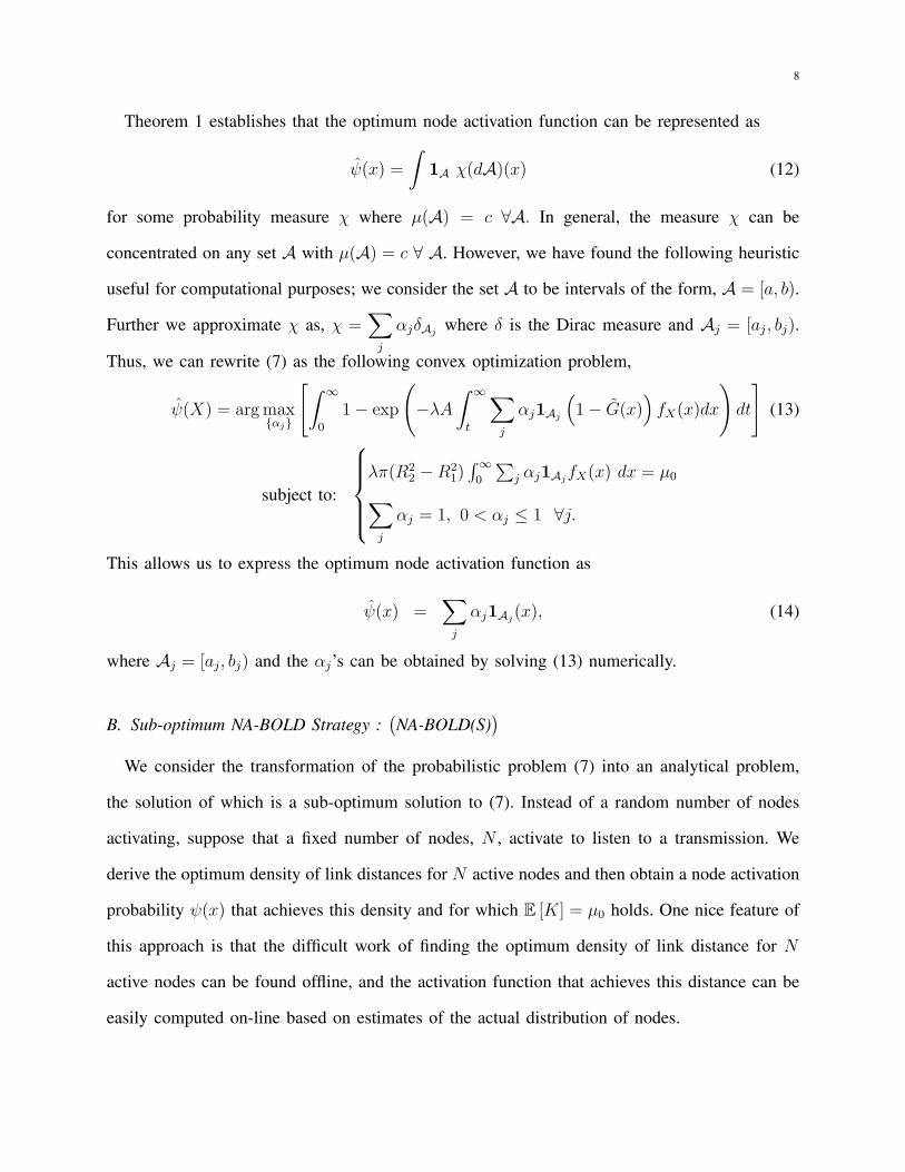
Theorem 1 establishes that the optimum node activation function can be represented as

ψ(x) =

∫1A χ(dA)(x) (12)

for some probability measure χ where µ(A) = c ∀A. In general, the measure χ can be

concentrated on any set A with µ(A) = c ∀ A. However, we have found the following heuristic

useful for computational purposes; we consider the set A to be intervals of the form, A = [a, b).

Further we approximate χ as, χ =∑j

αjδAjwhere δ is the Dirac measure and Aj = [aj, bj).

Thus, we can rewrite (7) as the following convex optimization problem,

ψ(X) = arg maxαj

[∫ ∞

0

1− exp

(−λA

∫ ∞

t

∑j

αj1Aj

(1− G(x)

)fX(x)dx

)dt

](13)

subject to:

λπ(R2

2 −R21)∫∞

0

∑j αj1Aj

fX(x) dx = µ0∑j

αj = 1, 0 < αj ≤ 1 ∀j.

This allows us to express the optimum node activation function as

ψ(x) =∑j

αj1Aj(x), (14)

where Aj = [aj, bj) and the αj’s can be obtained by solving (13) numerically.

B. Sub-optimum NA-BOLD Strategy :(NA-BOLD(S)

)We consider the transformation of the probabilistic problem (7) into an analytical problem,

the solution of which is a sub-optimum solution to (7). Instead of a random number of nodes

activating, suppose that a fixed number of nodes, N , activate to listen to a transmission. We

derive the optimum density of link distances for N active nodes and then obtain a node activation

probability ψ(x) that achieves this density and for which E [K] = µ0 holds. One nice feature of

this approach is that the difficult work of finding the optimum density of link distance for N

active nodes can be found offline, and the activation function that achieves this distance can be

easily computed on-line based on estimates of the actual distribution of nodes.

9

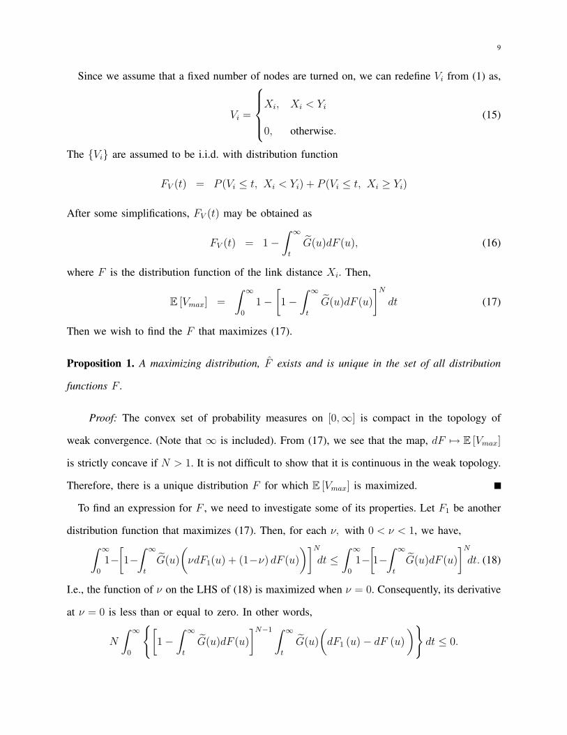
Since we assume that a fixed number of nodes are turned on, we can redefine Vi from (1) as,

Vi =

Xi, Xi < Yi

0, otherwise.(15)

The Vi are assumed to be i.i.d. with distribution function

FV (t) = P (Vi ≤ t, Xi < Yi) + P (Vi ≤ t, Xi ≥ Yi)

After some simplifications, FV (t) may be obtained as

FV (t) = 1−∫ ∞

t

G(u)dF (u), (16)

where F is the distribution function of the link distance Xi. Then,

E [Vmax] =

∫ ∞

0

1−[1−

∫ ∞

t

G(u)dF (u)

]Ndt (17)

Then we wish to find the F that maximizes (17).

Proposition 1. A maximizing distribution, F exists and is unique in the set of all distribution

functions F .

Proof: The convex set of probability measures on [0,∞] is compact in the topology of

weak convergence. (Note that ∞ is included). From (17), we see that the map, dF 7→ E [Vmax]

is strictly concave if N > 1. It is not difficult to show that it is continuous in the weak topology.

Therefore, there is a unique distribution F for which E [Vmax] is maximized.

To find an expression for F , we need to investigate some of its properties. Let F1 be another

distribution function that maximizes (17). Then, for each ν, with 0 < ν < 1, we have,∫ ∞

0

1−[1−∫ ∞

t

G(u)

(νdF1(u) + (1−ν) dF (u)

)]Ndt ≤

∫ ∞

0

1−[1−∫ ∞

t

G(u)dF (u)

]Ndt. (18)

I.e., the function of ν on the LHS of (18) is maximized when ν = 0. Consequently, its derivative

at ν = 0 is less than or equal to zero. In other words,

N

∫ ∞

0

[1−

∫ ∞

t

G(u)dF (u)

]N−1 ∫ ∞

t

G(u)

(dF1 (u)− dF (u)

)dt ≤ 0.

10

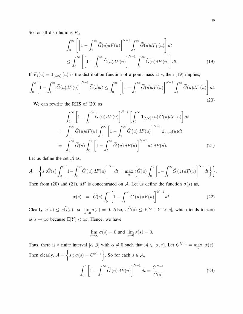
So for all distributions F1,∫ ∞

0

[[1−

∫ ∞

t

G(u)dF (u)

]N−1 ∫ ∞

t

G(u)dF1 (u)

]dt

≤∫ ∞

0

[[1−

∫ ∞

t

G(u)dF (u)

]N−1 ∫ ∞

t

G(u)dF (u)

]dt. (19)

If F1(u) = 1[s,∞] (u) is the distribution function of a point mass at s, then (19) implies,∫ s

0

[1−

∫ ∞

t

G(u)dF (u)

]N−1

G(s)dt ≤∫ ∞

0

[[1−

∫ ∞

t

G(u)dF (u)

]N−1 ∫ ∞

t

G(u)dF (u)

]dt.

(20)We can rewrite the RHS of (20) as∫ ∞

0

[1−

∫ ∞

t

G (u) dF (u)

]N−1 [∫ ∞

0

1[t,∞] (u) G(u)dF (u)

]dt

=

∫ ∞

0

G(u)dF (u)

∫ ∞

0

[1−

∫ ∞

t

G (u) dF (u)

]N−1

1[t,∞](u)dt

=

∫ ∞

0

G(u)

∫ u

0

[1−

∫ ∞

t

G (u) dF (u)

]N−1

dt dF (u). (21)

Let us define the set A as,

A =

s :G(s)

∫ s

0

[1−∫ ∞

t

G (u) dF (u)

]N−1

dt = maxu

G(u)

∫ u

0

[1−∫ ∞

t

G (z) dF (z)

]N−1

dt

.

Then from (20) and (21), dF is concentrated on A. Let us define the function σ(s) as,

σ(s) = G(s)

∫ s

0

[1−

∫ ∞

t

G (u) dF (u)

]N−1

dt. (22)

Clearly, σ(s) ≤ sG(s), so lims→0

σ(s) = 0. Also, sG(s) ≤ E[Y : Y > s], which tends to zero

as s→∞ because E[Y ] <∞. Hence, we have

lims→∞

σ(s) = 0 and lims→0

σ(s) = 0.

Thus, there is a finite interval [α, β] with α 6= 0 such that A ∈ [α, β]. Let CN−1 = maxs

σ(s).

Then clearly, A =

s : σ(s) = CN−1

. So for each s ∈ A,

∫ s

0

[1−

∫ ∞

t

G (u) dF (u)

]N−1

dt =CN−1

G(s)(23)

11

Note that in (23), both F and C are unknown. Let us assume for the moment that A is an

interval [α, β]. Differentiating (23) leads to

1−∫ β

s

G(u)dF (u) = C

[−G′(s)

(G(s)

)−2] 1

N−1

(24)

for every α ≤ s ≤ β. Let us now define

K(s) =

−G′(s)/

[G(s)

]2 1N−1

. (25)

Using integration by parts, we can rewrite (24) as

1 +

∫ ∞

s

g′(u)F (u)du+ F (s)G(s) = CK(s) (26)

To formalize our approach further, we impose the following (mild) conditions on G.

Hypothesis 1. G is twice continually differentiable and bounded away from zero on compact

sets.

Applying this hypothesis, (26) shows that F is differentiable, so that dF (u) = f(u)du. Using

this in (24) and differentiating,

f(s) = CK′(s)G(s)

, α ≤ s ≤ β (27)

Note that we have still not identified C, α and β in (27). Substituting (27) into (24),

1− C

∫ β

s

K′(u)du = CK(s) ⇒ CK(β) = 1. (28)

We also have∫ βαdF (u) = 1, which implies that

C

∫ β

α

K′(s)G(s)

ds = 1. (29)

Recall that we have assumed A = [α, β] before. Thus, for α ≤ s ≤ β, we can rewrite (23) as,∫ s

0

[1−

∫ β

t∨αG (u) f(u)du

]N−1

dt =CN−1

G(s). (30)

Using the definition of K(s) in (30) and then applying (28), we have for α ≤ s ≤ β,

α [1− CK(β) + CK(α)]N−1 +

∫ s

α

[1− CK(β) + CK(t)]N−1 dt =CN−1

G(s). (31)

12

Applying (28) to (31), we obtain,

α [CK(α)]N−1 +

∫ s

α

CN−1K(t)N−1dt =CN−1

G(s). (32)

Using the definition of K(s) in (32) and simplifying, we have for α ≤ s ≤ β,

α [CK(α)]N−1 + CN−1

∫ s

α

d

du

(1

G(u)

)du =

CN−1

G(s).

Some algebra yields α [K(α)] = G−1(α), which implies(−G′(α)

)= G (α) (33)

The following lemma provides sufficient conditions on G for α, β and C, to be unique.

Lemma 1. Suppose G(s) = exp (−ϕ(s)) , where ϕ(0) = 0, ϕ > 0, ϕ′ is strictly increasing,

continuous and ϕ′(∞) > 0. Then (28), (29) and (33) determine α, β, C uniquely.

See Appendix for the proof. It remains to prove that α, β, C and f (given by (27)) is indeed

the solution to our problem. For that purpose, it is sufficient to prove the following theorem.

Theorem 2. Let α, β, C and f be defined as above. Then (23) holds and σ(s) ≤ CN−1,

where σ(s) has been defined in (22).

See Appendix for the proof.

The optimum density for a fixed number of nodes turning on can be used to find a suboptimal

node activation function ψ(x) for the probabilistic node activation problem (7). ψ(x) is chosen

so that the conditional distribution of the link distance to receiver i, given that receiver i is active,

achieves the desired distribution of node distances and the constraint on the expected number

of nodes that activates is met with equality. Thus, FXi(x| ζi = 1) = F (x),

P (Xi ≤ x ∩ ζi = 1)

P (ζi = 1)= F (x)∫ x

0ψ(u)fXi

(u) du∫∞0ψ(u)fXi

(u) du=

∫ x

0

f(t)dt.

Thus,

ψ(x) =fXi

(x)

fXi(x)

∫ ∞

0

ψ(u)fXi(u) du. (34)

13

is the unique solution (except on a set of measure zero, and up to a scaling factor). Let ψ(x) =

M−1f(x)/fXi(x), where

M = λπ(R2

2 −R21

)/µ0, and M ≥ 1 (35)

to satisfy the constraints in (7). Since ψ(x) is a conditional probability ψ(x) ≤ 1 imposes a

lower bound on λ. If we denote λ as the minimum density of nodes needed to be deployed for

which the expected number of nodes that turn on is µ0, then

λ =µ0

π (R22 −R2

1)max

R1<x≤R2

f(x)(fXi

(x))−1 (36)

IV. OUTAGE PROBABILITY FOR GEOGRAPHIC TRANSMISSION SCHEMES

Outage occurs if no active receiver recovers the message, i.e., Vmax = 0. The conditions that

can lead to outage are 1) no nodes are available in the network to receive the transmission

(ℵ = 0), 2) nodes are present physically but every node is powered off, or 3) the received SNR

falls below the threshold at every active node, (γi < ρ ∀i). Using (3), the outage probability pout

is pout = P (Vmax ≡ 0) = exp λA [FVi(0)− 1].

V. RAYLEIGH CHANNEL MODEL

For Rayleigh fading Hi are i.i.d. exponential random variables with mean 1. Thus G(y) =

exp (−ρyn)1[y>0](y), which satisfies the conditions of Lemma 1. Using(28), (29), and (33), the

optimum density of link distances, f(x) on R1 < x ≤ R2 is

f(x) =1

(N − 1)Rn−1N−1

2 exp(ρRn

2

N−1

)x n−1N−1 exp

(ρ

N

N − 1xn)[

n− 1

x+ nρxn−1

], and

ψ(x) =1

M

(R22 −R2

1)

2(N − 1)Rn−1N−1

2 exp(ρRn

2

N−1

)xn−NN−1 exp

(ρ

N

N − 1xn)[

n− 1

x+ nρxn−1

]. (37)

Here, R1 ≡ α = n

√(nρ)−1, R2 ≡ β is found numerically by solving the integral equation∫ R2

R1

f(x)dx = 1,

and M is given by (35).

14

The distribution function F (x) for the NA-BOLD(S) scheme is necessary to evaluate the

outage probability analytically and is given by

F (x) = c1n− 1

ng

(x;ω;

n− 1

n(N − 1);Nn− 1

n(N − 1)

)+ ρc1g

(x;ω;

Nn− 1

n(N − 1);2Nn− n− 1

n(N − 1)

),

where

g (x;ω; a, b) = B (1, a) xa 1F1 (a, b, ωxn)−B (1, b) Ra1 1F1 (a, b, ωRn

1 )

c1 =

((N − 1)R

n−1N−1

2 exp

(ρ

Rn2

N − 1

)), and

ω = ρN (N − 1)−1 .

Here, B(x, y) is the beta function, defined as,

B(x, y) =

∫ 1

0

ux−1(1− u)y−1du

and 1F1 (a; b; z) is the confluent hypergeometric function of the first kind, defined as,

1F1 (a; b; z) =Γ(b)

Γ(b− a)Γ(a)

∫ 1

0

exp (zt) ta−1(1− t)b−a−1 dt

The outage probability is then

pout = exp

(− µ0

(n− 1

nc1g

(x;ω

N;Nn− 1

n(N − 1)

)+ ρc1g

(x;ω

N;Nn− 1

n(N − 1);2Nn− n− 1

n(N − 1)

))).

VI. GEOGRAPHIC TRANSMISSION WITH CONSTANT NODE ACTIVATION PROBABILITIES

For the purpose of comparing our NA-BOLD approach with conventional schemes that employ

fixed node activation techniques, we consider the following strategies. These schemes have the

same objective and constraints as NA-BOLD schemes, but have an activation function that is

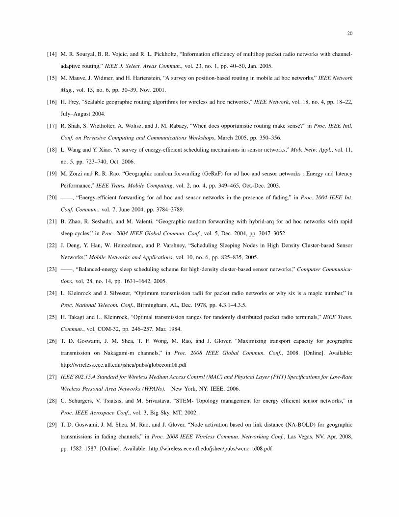
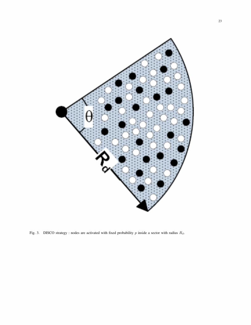
constant out to a fixed radius from the transmitter (and zero beyond that), as shown in Fig.3.

Consider first a simple strategy in which all nodes inside a sector around the transmitter up to

a fixed distance are awake to receive the transmission; i.e. P (ζi = 1) = p ≡ 1 ∀i as shown

in Fig.2. We refer to this strategy as the DISC strategy.

15

A more sophisticated strategy is to turn on nodes with a fixed probability p out to a larger radius

than the DISC scheme, where this radius is obtained to satisfy the constraint that the expected

number of nodes that activate is µ0. Letting ψ(x) = p, 0 < x ≤ Rd, with R1 = 0, R2 = Rd in (7),

we obtain,

p = arg maxp

[∫ ∞

0

1− exp

(−λAp

∫ ∞

t

(1− G(x)

)fX(x)dx

)dt

](38)

subject to:

λπR2

dp = µ0

0 ≤ p ≤ 1.

We refer to this scheme as the Optimized-DISC strategy (DISCO). For the Rayleigh fading

channel, the objective function is

p = arg maxp

[∫ Rd

0

1− exp

(−2πλ

n n√ρp

(γ

(2

n, ρRn

d

)− γ

(2

n, ρtn

)))dt

].

The outage probability for this scheme is

pout = exp

(−λπR2

d

p

R2d

(1

ρ

) 2n 2

nγ

(2

n, ρRn

2

)).

VII. RESULTS

In this section, we present the performance of the DISC, DISC-O, and NA-BOLD schemes. All

results presented are for a Rayleigh fading channel with path-loss exponent n = 4. The receive

SNR threshold is ρ = 1, and the node density is λ = 10 nodes per unit sector. The NA-BOLD

approach turns on nodes located inside a sector annulus, as shown in Fig. 1. The expected number

of nodes that turn on is µ0. The NA-BOLD(S) scheme is based on N = dµ0e, which is found

to offer good performance (N = dµ0 − 1e, which maximizes the Poisson pmf offers nearly the

same performance [29]). For the NA-BOLD(O) scheme, we obtained the optimum node activation

function using a piece-wise linear approximation with the help of the αj’s numerically obtained

by solving (13). The node activation probability for the sub-optimum NA-BOLD(S) scheme is

given in (37).

16

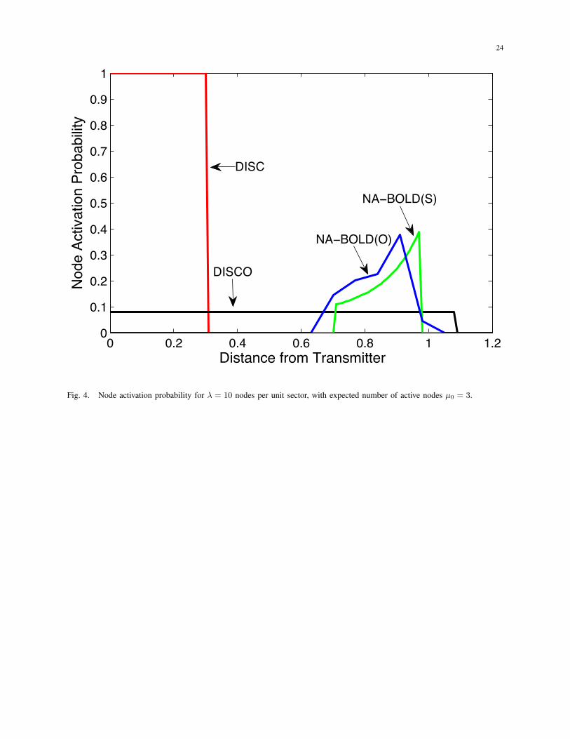
The node activation functions for the various schemes are shown as a function of distance

from the transmitter in Fig. 4 for µ0 = 3. For the NA-BOLD(S) scheme, R1 = 0.7071 for any µ0,

and we numerically found R2 = 0.8825 for µ0 = 3. The corresponding values for the optimum

scheme, NA-BOLD(O) are 0.63 and 0.84 respectively.

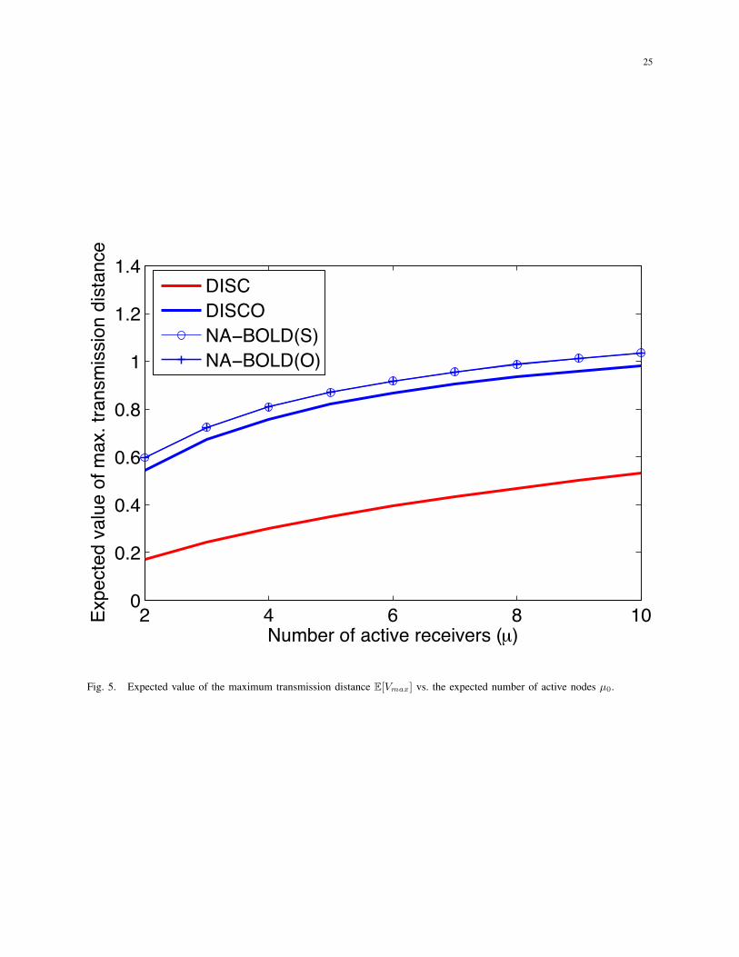
The expected values of the maximum transmission distance to the farthest receiver that

successfully received the transmission are shown in Fig. 5. The sub-optimum NA-BOLD(S)

scheme show almost identical performance to the optimal NA-BOLD(O) scheme. We provide

Table IX in order to evaluate how close this performance is, relative to the optimal scheme. We

find that the sub-optimal scheme performs within 1% of the optimal scheme for 2 ≤ µ0 ≤ 10.

For this range of µ0, the NA-BOLD schemes significantly outperform the conventional schemes

that employ fixed node activation. In particular, the NA-BOLD approach is better than the DISC

scheme by more than 100%. The DISCO scheme is within 9.5% to 5.5% of NA-BOLD for

µ0 = 3 to 10. In a practical MPRN, the number of nodes that turn on in is typically less than

6.0 [24] and hence NA-BOLD schemes might be better suited for such scenarios.

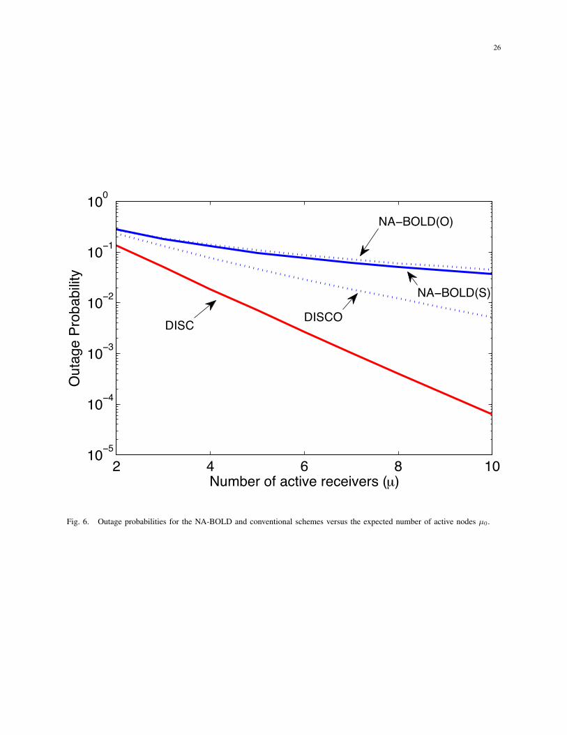
The outage probabilities are plotted in Fig. 6. Since outage is less likely to occur when

more nodes are present, the curves are decreasing functions of µ0. The DISC schemes have

relatively lower outage probabilities as they turn on more nodes that are located closer to the

transmitter. The NA-BOLD(S) shows a slight degradation in outage performance with respect

to NA-BOLD(O). However, this degradation is nominal – when the number of active nodes

is as high as 10, the outage probabilities are 4.5% and 3.6%, for the NA-BOLD(O) and the

NA-BOLD(S) schemes respectively.

VIII. CONCLUSIONS

In this paper, we propose node activation schemes that use distance to increase the expected

transmission distance for geographic transmissions over fading channels. Optimal and suboptimal

node activation schemes are developed and compared. Node activation based on link-distance

offers significant performance schemes over conventional approaches that activate nodes with

17

equal probabilities. The suboptimal scheme that gives a node-activation function in closed form,

yields performance close to the optimal scheme.

IX. APPENDIX

Proof of Lemma 1: The uniqueness of α and C are trivial if there is a unique β. From

(28) and (29), ∫ β

α

K′(s)G(s)

ds = K(β). (39)

For a given α, (39) has a unique solution. From (25),

K(s) =

[d

ds

(1

G(s)

)] 1N−1

= [ϕ′ (s) exp (ϕ (s))]1

N−1

Since ϕ′ and ϕ are increasing, K is strictly increasing, so K′ > 0. Since ϕ′(∞) > 0, ϕ(∞) = ∞,

and K(∞) = ∞. By assumption,1

G(s)is increasing and tends to infinity. Consider the funcion,

τ(s) =1

K(s)

∫ s

α

K′(u)G(u)

du, s ≥ α.

Then, τ(α) = 0 and for any s and t, s > t , we have,

τ(s) =1

K(s)

∫ t

α

K′(u)G(u)

du+1

K(s)

∫ s

t

K′(u)G(u)

du

>1

K(s)

∫ t

α

K′(u)G(u)

du+1

G(t)K(s)

∫ s

t

K′(u)du

=1

K(s)

∫ t

α

K′(u)G(u)

du+1

G(t)K(s)[K(s)−K(t)] . (40)

Since K(∞) = ∞, letting s→∞ in (39) we see τ(∞) >1

G(t)for any t, i.e. τ(∞) = ∞ and

τ(s) is strictly increasing in s. Since τ(α) = 0, there is a unique β such that τ(β) = 1. This

proves that a unique β satisfies (29).

18

Proof of Theorem 2: Using (27) and (28) we find,

∫ s

0

(1−∫ β

t∨αG(u)f(u)du

)N−1

dt =

CN−1s

(−G′(α)

(G(α)

)−2), 0 ≤ s ≤ α

CN−1α

(−G′(α)

(G(α)

)−2)

+CN−1

([G(s)

]−1

−[G(α)

]−1), α ≤ s ≤ β

CN−1[G(β)

]−1

+ s− β, s > β.

(41)

Applying (23) to (41), note that this is equivalent to proving

1

G(s)≥

s

(−G′(α)

(G(α)

)−2), 0 ≤ s ≤ α

α

(−G′(α)

(G(α)

)−2)

+

([G(s)

]−1

−[G(α)

]−1), α ≤ s ≤ β[

G(β)]−1

+ s− β, s > β.

(42)

We consider the three cases separately as follows.

Case 1, 0 ≤ s ≤ α: We need to prove that s − G′(α)(G(α)

)−2

≤(G(s)

)−1

Using (33), it

follows that we need to show,sg(s)

αG(α)≤ 1. (43)

Notice thatd

ds

[sG(s)

]= G(s) + sG′(s) = G(s)s

[1

s+G′(s)

G(s)

]> 0, 0 ≤ s ≤ α

We know from (33) that α−1 is a unique solution of α−1 + G′(α)/G(α) = 0. Since s−1 +

G′(s)/G(s) → ∞ as s → 0, it follows that, s−1 + G′(s)/G(s) is greater than or equal to zero

if 0 ≤ s ≤ α and less than 0 if s > α. Thus, sG(s) is increasing in 0 ≤ s ≤ α, implying (43).

Hence, the case 0 ≤ s ≤ α is proved.

Case 2, α < s ≤ β: Using (33) we see that the RHS of (42) in this case reduces to CN−1/G(s),

as required.

Case 3, s > β: We need to prove that CN−1/G(β) + s− β ≤ CN−1/G(s) or

CN−1

[1

G(β)− 1

G(s)

]+ s− β ≤ 0. (44)

19

Differentiating the LHS of (44) w.r.t. s, we have, CN−1G′(s)[G(s)

]−2

+1, which we can rewrite

as 1−CN−1(−G′(s)

) [G(s)

]−2

. Substituting the value of K(s) from (25) into this expression,

we obtain, 1 − [CK(s)]N−1. Since K′(s) > 0, K(s) is strictly increasing and using (28), we

have, 1− [CK(s)]N−1 ≤ 0, for s ≥ β. Thus the derivative of the function in the LHS of (44)

is ≤ 0, i.e. this function is decreasing and it vanishes at s = β. Hence the case s > β is proved.

REFERENCES

[1] R. Knopp and P. A. Humblet, “Information capacity and power control in single-cell multiuser communications,” in Proc.

1995 IEEE Int. Conf. Commun., vol. 1, Seattle, June 1995, pp. 331–335.

[2] P. Black, M. Grob, R. Padovani, N. Sindhushyana, and S. Viterbi, “CDMA/HDR : a bandwidth efficient high speed wireless

data service for nomadic users,” IEEE Commun. Mag., vol. 38, pp. 70–77, July 2000.

[3] B. Sadeghi, V. Kanodia, A. Sabharwal, and E. Knightly, “Opportunistic media access for multirate ad hoc networks,” in

Proc. MobiCom ’02. New York, NY, USA: ACM, 2002, pp. 24–35.

[4] J. Wang, H. Zhai, Y. Fang, and J. M. Shea, “OMAR: Utilizing diversity in wireless ad hoc networks,” IEEE Trans. Mobile

Computing, vol. 5, pp. 1764–1779, Dec. 2006.

[5] M. Grossglauser and D. Tse, “Mobility increases the capacity of ad hoc wireless networks,” IEEE/ACM Trans. Networking,

vol. 10, pp. 477–486, August 2002.

[6] P. Larsson, “Selection diversity forwarding in a multihop packet radio network with fading channel and capture,” in ACM

SIGMOBILE Mobile Computing and Communication Review, Oct. 2001, pp. 47–54.

[7] M. Zorzi and R. R. Rao, “Geographic random forwarding (GeRaF) for ad hoc and sensor networks : Multihop performance,”

IEEE Trans. Mobile Computing, vol. 2, no. 4, pp. 337–348, Oct.-Dec. 2003.

[8] M. Valenti and N. Correal, “Exploiting macrodiversity in dense multihop networks and relay channels,” in Proc. IEEE

Wireless Commun. and Networking, Mar. 2003.

[9] W.-H. Wong, J. M. Shea, and T. F. Wong, “Cooperative diversity slotted ALOHA,” Wireless Networks, vol. 13, pp.

361–369, June 2007. [Online]. Available: http://wireless.ece.ufl.edu/jshea/pubs/winet05.pdf

[10] ——, “Cooperative diversity slotted ALOHA,” in Proc. 2nd Int. Conf on Quality of Service in Heterogeneous Wired/Wireless

Networks (QShine), Orlando, Florida, Aug. 2005, pp. 8.4.1–8.

[11] S. Biswas and R. Morris, “Exor: opportunistic multi-hop routing for wireless networks,” SIGCOMM Comput. Commun.

Rev., vol. 35, no. 4, pp. 133–144, 2005.

[12] J. Jubin and J. Tornow, “The darpa packet radio network protocols,” Proc. IEEE, vol. 75, no. 1, pp. 21–32, Jan. 1987.

[13] P. Larsson and N. Johansson, “Multiuser diversity forwarding in multihop packet radio networks,” in Proc. IEEE Wireless

Commun. and Networking Conf., vol. 4, 2005, pp. 2188–2194.

20

[14] M. R. Souryal, B. R. Vojcic, and R. L. Pickholtz, “Information efficiency of multihop packet radio networks with channel-

adaptive routing,” IEEE J. Select. Areas Commun., vol. 23, no. 1, pp. 40–50, Jan. 2005.

[15] M. Mauve, J. Widmer, and H. Hartenstein, “A survey on position-based routing in mobile ad hoc networks,” IEEE Network

Mag., vol. 15, no. 6, pp. 30–39, Nov. 2001.

[16] H. Frey, “Scalable geographic routing algorithms for wireless ad hoc networks,” IEEE Network, vol. 18, no. 4, pp. 18–22,

July–August 2004.

[17] R. Shah, S. Wietholter, A. Wolisz, and J. M. Rabaey, “When does opportunistic routing make sense?” in Proc. IEEE Intl.

Conf. on Pervasive Computing and Communications Workshops, March 2005, pp. 350–356.

[18] L. Wang and Y. Xiao, “A survey of energy-efficient scheduling mechanisms in sensor networks,” Mob. Netw. Appl., vol. 11,

no. 5, pp. 723–740, Oct. 2006.

[19] M. Zorzi and R. R. Rao, “Geographic random forwarding (GeRaF) for ad hoc and sensor networks : Energy and latency

Performance,” IEEE Trans. Mobile Computing, vol. 2, no. 4, pp. 349–465, Oct.-Dec. 2003.

[20] ——, “Energy-efficient forwarding for ad hoc and sensor networks in the presence of fading,” in Proc. 2004 IEEE Int.

Conf. Commun., vol. 7, June 2004, pp. 3784–3789.

[21] B. Zhao, R. Seshadri, and M. Valenti, “Geographic random forwarding with hybrid-arq for ad hoc networks with rapid

sleep cycles,” in Proc. 2004 IEEE Global Commun. Conf., vol. 5, Dec. 2004, pp. 3047–3052.

[22] J. Deng, Y. Han, W. Heinzelman, and P. Varshney, “Scheduling Sleeping Nodes in High Density Cluster-based Sensor

Networks,” Mobile Networks and Applications, vol. 10, no. 6, pp. 825–835, 2005.

[23] ——, “Balanced-energy sleep scheduling scheme for high-density cluster-based sensor networks,” Computer Communica-

tions, vol. 28, no. 14, pp. 1631–1642, 2005.

[24] L. Kleinrock and J. Silvester, “Optimum transmission radii for packet radio networks or why six is a magic number,” in

Proc. National Telecom. Conf., Birmingham, AL, Dec. 1978, pp. 4.3.1–4.3.5.

[25] H. Takagi and L. Kleinrock, “Optimal transmission ranges for randomly distributed packet radio terminals,” IEEE Trans.

Commun., vol. COM-32, pp. 246–257, Mar. 1984.

[26] T. D. Goswami, J. M. Shea, T. F. Wong, M. Rao, and J. Glover, “Maximizing transport capacity for geographic

transmission on Nakagami-m channels,” in Proc. 2008 IEEE Global Commun. Conf., 2008. [Online]. Available:

http://wireless.ece.ufl.edu/jshea/pubs/globecom08.pdf

[27] IEEE 802.15.4 Standard for Wireless Medium Access Control (MAC) and Physical Layer (PHY) Specifications for Low-Rate

Wireless Personal Area Networks (WPANs). New York, NY: IEEE, 2006.

[28] C. Schurgers, V. Tsiatsis, and M. Srivastava, “STEM- Topology management for energy efficient sensor networks,” in

Proc. IEEE Aerospace Conf., vol. 3, Big Sky, MT, 2002.

[29] T. D. Goswami, J. M. Shea, M. Rao, and J. Glover, “Node activation based on link distance (NA-BOLD) for geographic

transmissions in fading channels,” in Proc. 2008 IEEE Wireless Commun. Networking Conf., Las Vegas, NV, Apr. 2008,

pp. 1582–1587. [Online]. Available: http://wireless.ece.ufl.edu/jshea/pubs/wcnc td08.pdf

21

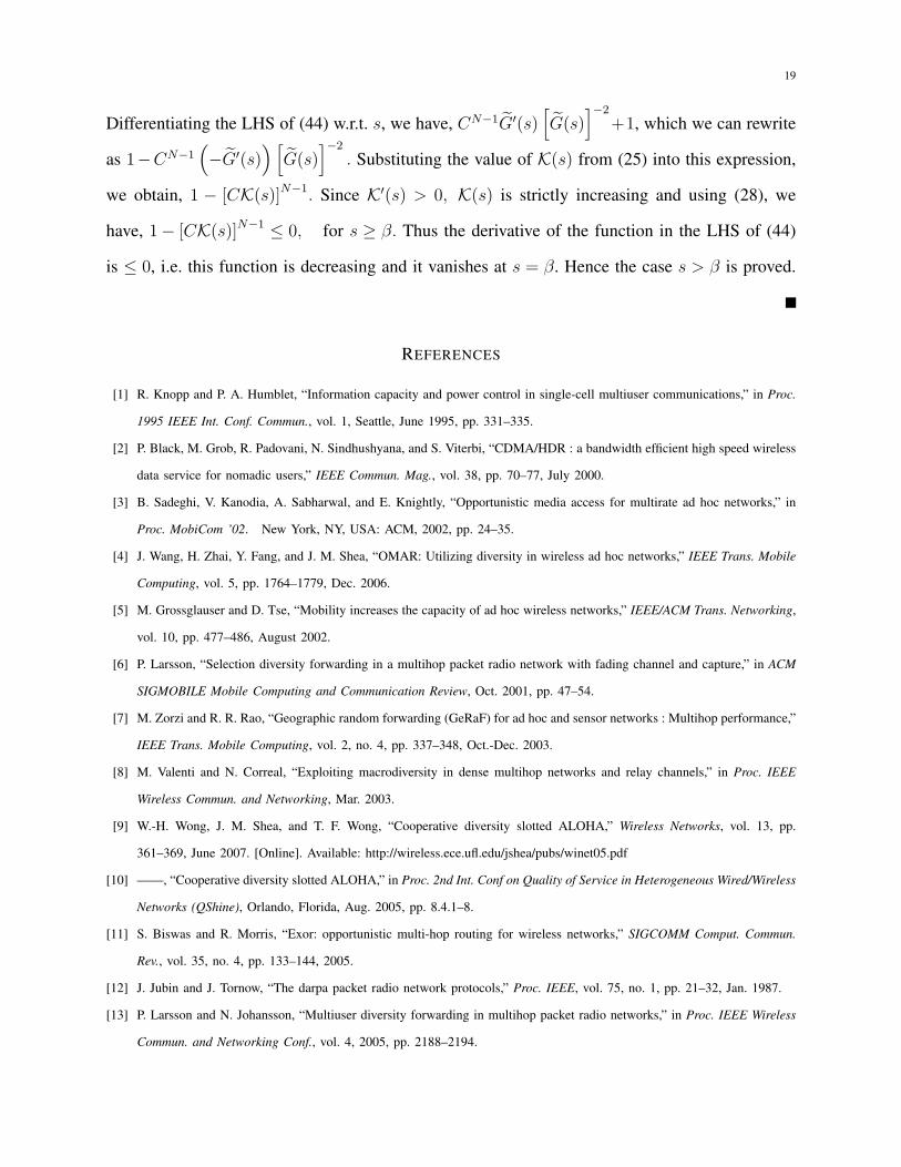
Fig. 1. Geographic Transmission region : annulus of a sector with inner radius R1, outer radius R2 with transmitter at center.

22

Fig. 2. DISC strategy : all nodes are activated inside a sector with radius radius Rd.

23

Fig. 3. DISCO strategy : nodes are activated with fixed probability p inside a sector with radius Rd.

24

0 0.2 0.4 0.6 0.8 1 1.20

0.1

0.2

0.3

0.4

0.5

0.6

0.7

0.8

0.9

1

Distance from Transmitter

Node

Act

ivatio

n Pr

obab

ility

NA−BOLD(S)

NA−BOLD(O)

DISCO

DISC

Fig. 4. Node activation probability for λ = 10 nodes per unit sector, with expected number of active nodes µ0 = 3.

25

2 4 6 8 100

0.2

0.4

0.6

0.8

1

1.2

1.4

Number of active receivers (µ)

Expe

cted

val

ue o

f max

. tra

nsm

issio

n di

stan

ce

DISCDISCONA−BOLD(S)NA−BOLD(O)

Fig. 5. Expected value of the maximum transmission distance E[Vmax] vs. the expected number of active nodes µ0.

26

2 4 6 8 1010−5

10−4

10−3

10−2

10−1

100

Number of active receivers (µ)

Out

age

Prob

abilit

y

DISC DISCO

NA−BOLD(O)

NA−BOLD(S)

Fig. 6. Outage probabilities for the NA-BOLD and conventional schemes versus the expected number of active nodes µ0.

27

TABLE I

EXPECTED VALUE OF MAXIMUM TRANSMISSION DISTANCE FOR VARIOUS NODE ACTIVATION SCHEMES

Constant node activation approach NA-BOLD Approach

µ DISC DISCO NA-BOLD(S) NA-BOLD(O)

2 0.1714 0.5455 0.5976 0.5989

3 0.2437 0.6718 0.7243 0.7247

4 0.3025 0.7580 0.8091 0.8097

5 0.3519 0.8201 0.8707 0.8713

6 0.3950 0.8677 0.9179 0.9186

7 0.4335 0.9049 0.9556 0.9565

8 0.4686 0.9351 0.9866 0.9875

9 0.5012 0.9602 1.0127 1.0135

10 0.5316 0.9814 1.0350 1.0356