Distinguishing Infections on Different GraphTopologies

Chris Milling, Constantine Caramanis, Shie Mannor and Sanjay Shakkottai∗

September 26, 2013

Abstract

The history of infections and epidemics holds famous examples where understand-ing, containing and ultimately treating an outbreak began with understanding its modeof spread. Influenza, HIV and most computer viruses, spread person to person, deviceto device, through contact networks; Cholera, Cancer, and seasonal allergies, on theother hand, do not. In this paper we study two fundamental questions of detection:first, given a snapshot view of a (perhaps vanishingly small) fraction of those infected,under what conditions is an epidemic spreading via contact (e.g., Influenza), distin-guishable from a “random illness” operating independently of any contact network(e.g., seasonal allergies); second, if we do have an epidemic, under what conditions is itpossible to determine which network of interactions is the main cause of the spread –the causative network – without any knowledge of the epidemic, other than the identityof a minuscule subsample of infected nodes?

The core, therefore, of this paper, is to obtain an understanding of the diagnosticpower of network information. We derive sufficient conditions networks must satisfyfor these problems to be identifiable, and produce efficient, highly scalable algorithmsthat solve these problems. We show that the identifiability condition we give is fairlymild, and in particular, is satisfied by two common graph topologies: the grid, and theErdos-Renyi graphs.

1 Introduction

People and devices routinely interact through multiple networks – contact networks – be theyvirtual, technological or physical, allowing the rapid exchange of ideas, fashions, rumors, but

∗C. Milling, C. Caramanis and S. Shakkottai are with the Department of Electrical and Com-puter Engineering, The University of Texas at Austin, USA, Emails: cmilling@utexas.edu,

constantine@utexas.edu, shakkott@austin.utexas.edu. S. Mannor is with the Department of Elec-trical Engineering, Technion, Israel, Email: shie@ee.technion.ac.il. This work was partially supportedby NSF Grants CNS-1017525, CNS-0721380, EFRI-0735905, EECS-1056028, DTRA grant HDTRA 1-08-0029 and Army Research Office Grant W911NF-11-1-0265. Early versions of this paper have appeared in theProceedings of ACM Sigmetrics, June 2012 [1], and the Proceedings of the 50th Annual Allerton Conferenceon Communication, Control, and Computing, October 2012 [2].

1

arX

iv:1

309.

6545

v1 [

cs.S

I] 2

5 Se

p 20

13

also viruses and disease. Throughout this paper we refer to anything that spreads over acontact network as an epidemic. Understanding if something is indeed an epidemic bestdescribed through contact-network spreading, and secondly, understanding the causativenetwork of that epidemic, is of critical important in many domains. Economists, sociologistsand marketing departments alike have long sought to understand how ideas, memes, fads andfashions, spread through social networks. Meanwhile, epidemiology has understood the valueof knowing the causative network of disease epidemics, from Influenza to HIV. Indeed, at onepoint, HIV was known as the “4H disease” where 4H referred to “Haitians, Homosexuals,Hemophiliacs, and Heroin users” [3, 4]. Understanding the causative network has greatlycontributed to controlling the worldwide spread of the virus.

While smartphone viruses have not yet supplanted computer viruses as the spreadingtechnological threat of the hour, their potential for broad destructive impact is clear. Justas different human viruses may have different dominant spreading networks (again, compareInfluenza and HIV), so may smartphone viruses spread over multiple networks, includingbluetooth, SMS/MMS messaging, or e-mail.

A first step towards containing epidemics, be they technological or physical, relies onproperly understanding the phenomenon as an epidemic in the first place, and then, accu-rately understanding the causative spread, before then adopting network-specific strategiesfor containment, quarantining and treatment.

Many factors complicate the process of determining the causative network. First, possiblybecause of long latency/hybernation periods, variation in reporting/detection, or simply lackof data, in some cases it may be difficult or impossible to collect accurate longitudinal data.Equally importantly, the reporting set of those “infected” (be they people or devices) maybe only a tiny fraction of those in fact infected. Therefore in this paper, we consider themost dire information regime: we assume we have data from only a single snapshot of time,where only a (perhaps vanishing) fraction of the infected population reports.

With these data, this paper focuses on determining the causative network for the spreadof an epidemic (e.g. virus, sickness, or opinion) from limited samples of the network state.

1.1 Setting and Results

We model people/devices/etc. as a set of nodes, V , of a graph. The nodes in V becomeinfected by an epidemic that spreads according to either graph G1 = (V,E1), or G2 = (V,E2),propagating along the edges of these graphs, according to an SI model of infection [5]. Givena (potentially small) sub-sample of the infected nodes at a single snapshot in time, ourobjective is to determine the network over which the epidemic is spreading. If one of thegraphs, say G2, is a star graph, where each node has a single edge to an external infectionsource, this models the problem of distinguishing an epidemic spreading on G1, from arandom illness spreading according to no network structure.

This paper is about understanding when the two processes – spreading on G1 or G2 – arestatistically distinguishable, and moreover when this can be done by an efficient algorithm.Evidently, in certain regimes, no algorithm can distinguish between the two processes. First,the graphs need to be sufficiently different. We quantify this precisely in Section 2. Beyondthis, certainly, if (almost) everyone is infected, or if (almost) none of those infected report,then nothing can be done. Our results are presented in terms of these two quantities: we

2

are interested in understanding the maximum number of nodes (people/devices) that canbe infected, and simultaneously the minimum number of these that actually report they areinfected, so that our algorithms correctly distinguish the true spreading process, with highprobability.

There are two regimes of graph topologies we consider: the setting where G2 is a stargraph – we call this the ‘infection vs. random sickness’ problem – and then the setting whereboth G1 and G2 exhibit nontrivial network structure – we call this the ‘graph comparison’problem. For the sake of the mathematical exposition, we find it more natural to presentfirst the graph comparison problem, and then the infection vs. random sickness problem.

We provide efficiently computable algorithms to answer the above questions, and thenprovide sufficient conditions on the regimes where our algorithms are guaranteed to succeed,with high probability. Specifically, our main contributions are as follows:

(i) Algorithm: We develop efficiently computable algorithms for both problems. Forinferring the causative network in the graph comparison problem, we develop whatwe call the Comparative Ball Algorithm. For the ‘infection vs. random sickness’,we develop two algorithms: the Threshold Ball Algorithm and the Threshold TreeAlgorithm. These algorithms build on the intuition that infected nodes are clusteredmore strongly on the true causative network. If on one network, the clustering istighter, it is more likely that it is driving the infection. We quantify clustering basedon the ball radius that contains the infected nodes.

(ii) Guarantees for General Graphs: For the graph comparison problem, we identifytwo natural graph conditions that we use to give very general performance guaran-tees for our Comparative Ball Algorithm. The first property is called the (a) Speedcondition; a graph satisfies this if the epidemic ball radius increases linearly in time.The second key property is called the (b) Spread condition; a graph satisfies this if arandomly selected collection of nodes are sufficiently spread apart, with respect to thenatural metric induced by the graph. For any two graphs that satisfy both (a) and (b),we derive upper bounds on the number of total infected nodes, and lower bounds onthe number of reporting nodes, so that our Comparative Ball Algorithm is guaranteedto correctly determine the causative network (as n→∞ and with high probability).

(iii) Grids and the Erdos-Renyi Random Graphs: For both d-dimensional grids,and the giant component of the Erdos-Renyi random graph (with constant asymptoticaverage degree), and for both the graph comparison and infection vs. random sicknessproblem, we derive bounds on the parameters associated with the speed and spreadconditions, thus, providing sufficient conditions on the regime where we can determinethe causative network.

1.2 Related Work

The infection model we consider in this paper is the susceptible-infected (SI) model wherenodes transition from susceptible to infected according to a memoryless process [5]. Much ofthe work on this model has focused on the predictive or analytic side, focused on character-izing the spread of the infection under various different settings. For example, [6] considers

3

graphs with multiple mixing distances (that is, local and global spreading), while [7] consid-ers the setting where the infected nodes are mobile. There are other approaches to modelinginfection, and while interesting to extend the current ideas and analysis there, we do notconsider these in the present work.

Our work, in contrast, lies on the inference side, where given (partial) information aboutthe realization of an epidemic, the goal is to infer various properties or parameters of thespreading process. While quite different in terms motivation and goals, a few recent workshave also considered epidemic inference. In [8], the authors provide a Bayesian inferenceapproach for estimating the transmission rates of the infection. Alternatively, one can useMCMC methods to estimate the model parameters [9], [10]. A similar problem is consideredin [11, 12], where, given a set of infected nodes, one seeks to determine which node is mostlikely to be the original source of the infection.

On the technical side, several of our results are related to first-passage percolation. In thefirst-passage percolation basic formulation, there is a (lattice) graph of infinite size. For eachedge, an independent random variable is generated that represents the time taken to traversethat edge. Some node is denoted as the source, and the time taken to reach another node isthe minimum of the total time to traverse a path over all paths between the source and thatdestination. This is equivalent to an infection traveling through the network as consideredhere. Work has been done to analyze various characterizing properties of this percolation,such as the shape of the infection and the rate at which it spreads. In the sequel, we findparticularly useful percolation results on trees [13] and lattices [14].

1.3 Outline of the Paper

The paper is organized as follows. In Section 2, we define precisely the infection model as wellour two main problems: determining the causative infection network between two graphs,and between a graph and a random sickness. Section 3 contains our analysis of the problemof distinguishing infections between two different graphs. We provide an efficient algorithm,and then the success criteria of this algorithm for distinguishing between epidemics on generalgraphs. We show that the sufficient conditions we provide are satisfied by a general classof graphs, that include two standard graph topologies, d-dimensional grids and Erdos-Renyigraphs. Then, in Section 4, we turn to the problem of distinguishing an infection from arandom sickness. Recall that this is equivalent to taking one of the two graphs to be thestar graph. Star graphs, however, do not have non-trivial neighborhoods, and hence thealgorithm and analysis from the previous part do not immediately carry over. We developtwo new algorithms for this setting, and provide success guarantees for each. We consider gridand Erdos-Renyi graphs. Finally, Section 5 contains the simulations data for each of theseproblems and illustrates the empirical performance of our algorithm on these graphs. Ourresults demonstrate that on synthetic data, empirical performance recovers the theoreticalresults. We also test our algorithms on a real-world graph, and our simulations show thathere too, our algorithms are quite effective.

4

2 The Model

We consider a collection of n nodes (vertices V ) which are members of two different networks(graphs). These graphs are denoted by G1 = (V,E1) and G2 = (V,E2); they share the samevertex set but have different edge sets. For example, G1 could represent the n verticesarranged on a d−dimensional grid, and G2 could be an Erdos-Renyi graph. Note that G2

does not need to have qualitatively different structure from G1: Indeed G2 could also be ad−dimensional grid, but with a different node-to-edge mapping.

2.1 Objective

We assume that the two graph topologies, G1 and G2 are known. At some point in time,an epidemic begins at a random node and spreads according to the edges of one of the twographs, following the infection model described below in Section 2.2. At some snapshot intime, a small random subset of the infected nodes report their infection. From the knowledgeof the graph topologies and the identity of the reporting nodes (but without knowledge ofthe other infected nodes) our objective is to design an algorithm that (asymptotically, as thesize of the problem scales) correctly determines which graph the epidemic is spreading on.

We first study the setting where both G1 and G2 have non-trivial neighborhoods, andthe goal is to detect which graph is responsible for spreading the epidemic; we call this theGraph Comparison Problem. We then consider the setting where G2 is the star graph, hencemodeling the problem of distinguishing an epidemic from a random illness.

2.2 Infection Model

We assume that an epidemic propagating on one of the two graphs, G1 or G2. The objective isto determine on which network it is spreading. We reiterate that this ‘epidemic’ could modelmany situations, including the spread of a cellphone virus, physical sickness of humans, andopinions or influence about products or ideas.

Given that the epidemic is on graph Gi, the spread occurs as follows (the standard SIdynamics [5]). A node is randomly selected to be the epidemic seed, and thus is the first“infected” node. At random times, the illness spreads from the sick nodes to some subset ofthe neighbors of the sick nodes, according to an exponential process. Specifically, associatean independent mean 1 exponential random variable with each edge incident to an infectedand an uninfected (a susceptible) node. The realization of this random variable representsthe transit time of the infection across that specific edge – a random variable. Thus aninfected node proceeds to infect its neighbors, with each non-infected neighbor becominginfected after the random transit time associated with the edge between the infected nodeand this neighbor. This process proceeds until the entire graph Gi is infected.

If the graph is a star graph, then every node is incident to a single external node. Con-sequently, nodes become sick at the same rate, and independently of every other node. Thisprocess, then, is stochastically equivalent to a random illness, where by a given time t, eachnode has become sick independently with some fixed probability q.

In either case, the infection continues until some (unknown) time t. At this time, asub-sample of the infected nodes report their infection state independently, each with some

5

probability q < 1. We let S denote the set of infected nodes, and Srep ⊆ S the set of reportinginfected nodes.1

2.3 Graph Structure

For the statistical problem of distinguishing the causative network to be well-posed, thecontact networks encoded by graphs G1 and G2 must be sufficiently different. Note thatthis does not imply that the topology of the graphs must be different (indeed, it could beidentical). Rather, the neighborhoods of each graph must be distinct, i.e., the nodes thatare near an infected node with respect to one graph, must be different from the nodes nearthe same infected node, with respect to the other graph. We note that if this is not the case,then both graphs encode approximately the same causative network, and hence solving thecomparative graph problem is not that important.

In this paper, we require that corresponding nodes on the two graphs have independentneighborhoods.2 It is easiest to explain this condition by means of a random construction,which is also the one we assume for the results in the sequel. Let G1 and G2 be graphs of thesame size n, whose nodes are unlabeled. Then randomly label the nodes of graph G1 from‘1’ to ‘n’ uniformly, and independently and uniformly at random label the nodes of graphG2. Nodes of the same label represent the same entity (person, device), i.e., if a node on onegraph is infected, the corresponding node on the other graph is also infected.

This independent neighborhood condition approximately holds in typical settings. Con-sider for instance the several hundred “nodes” (people, or devices) that come within blue-tooth range during a walk through the mall. This list likely has extremely small overlap(possibly only the few friends accompanying us on the mall excursion) with the set of nodesthat send us e-mail or SMS on a regular basis.

3 Graph Comparison Problem

The graph comparison problem consists of distinguishing the causative graph for an infectionspreading on one of two structured graphs G1 and G2. We make precise what we mean bystructured graphs below, but intuitively, both graphs have non-trivial neighborhood struc-ture, in contrast to the star graph. This is the key technical feature that differentiates thecomparative graph problem from the infection vs. random sickness problem, which we takeup in Section 4. As the algorithm reveals, the key in the comparative graph problem is that,under appropriate conditions, the infection, or epidemic, is clustered on either G1 or G2. Inthe case where G2 is the star graph, there is no notion of clustering there, so our algorithmsmust detect clustering vs. absence of clustering.

We turn to the details of the comparative graph problem. The first order of businessis understanding precisely what conditions we require the topology of graphs G1 and G2

to satisfy, making precise the notion of “non-trivial neighborhood structure” that, where,

1Note that we suppress the dependence of both S and Srep on n, unless required for clarity.2We note that we can envision other conditions based on clustering of epidemics on the two graphs which

also serves as alternate sufficient conditions. For simplicity, we restrict ourselves to the ‘random node index’condition in this paper.

6

unlike the star graph, an epidemic exhibits some statistically detectable clustering. Thereare two key properties required: first, the infection must spread at a bounded speed; second,a random collection of nodes on the graph must, with high probability, not exhibit a strongclustering. Of course, the star graph fails with respect to the minimum spread of randomnodes condition. As another example that fails the bounded speed condition, consider a treewhose nodes have degree dk+1 at level k.

We now state these conditions precisely, and in addition, we show, many graphs satisfythese conditions, including familiar topologies like the d-dimensional grid and the Erdos-Renyi graphs. It is also easy to see that any graph with bounded degree also satisfies thesetwo conditions.

We need first a simple definition:

Definition 1. Given a graph G = (V,E) and a subset of its nodes, S ⊆ V , let RadiusBall(G,S)denote the radius of the smallest ball that contains S. This can be computed in time at mostO(card(V )2).

Let G = G(n) denote a family of graphs, where G(n) denotes the subset of the graphs of Gthat have n nodes. For each n, there is a (possibly trivial) probability space

(G(n), σ(G(n)), P (n)

).

Concrete examples include the set of d-dimensional grid graphs, Erdos-Renyi graphs withbounded expected degree, d-regular trees, etc.

Definition 2. A family G satisfies the speed and spread conditions, if there exist constantssG, bG and βG, such that for any sequence G(n) picked randomly from the product probabilityspace

∏n G(n), the following hold with probability approaching 1 as n increases, where the

probability is over the random subset of nodes in the definitions below, and, in the case ofrandom families, G, such as Erdos-Renyi graphs, over the selection of G(n) as well:

Speed Condition: For infections starting at a randomly selected nodes and infectiontimes t(n) →∞, the set S(n) of nodes infected at time t(n) satisfies RadiusBall(G(n), S(n)) <sGt

(n).

Spread Condition: First, diam(G(n) = Ω(log n). Second, a random set S(n) of nodesof G(n), with card(S(n)) > βG log n, satisfies RadiusBall(G(n), S(n)) > bGdiam(G(n)).

These two conditions essentially encode the properties required so that an infectionspreading on a graph G

(n)1 (chosen from family G1) exhibits clustering, and, conversely, if it

is spreading on another graph G(n)2 (chosen from family G2) with independent neighborhoods

(as described above) then there is no clustering with respect to G(n)1 .

Note that to ease notation, whenever the context is clear, we drop the superscript (n)that denotes the number of nodes.

3.1 The Comparative Ball Algorithm

We provide an algorithm for the Comparative Graph Problem, called the Comparative BallAgorithm, and then give a theorem with sufficient conditions guaranteeing its success. Thealgorithm is natural, given the discussion above. We find the smallest ball on that graph that

7

contains all the reporting infected nodes. We take the ratio of the radius of this ball to thatof the graph’s diameter. These ratios – called the score of each graph – serve as a topologyindependent measure of clustering on each graph. The Comparative Ball Algorithm returnsthe graph with the smallest normalized clustering ratio. This is formally described below.

To specify our algorithm precisely, we require the following definitions. Given a graph G,a node v, and a radius r, we denote by Ballv,r(G) the collection of all nodes on the graph Gthat are at most a distance r from node v (graph distance measured by hop-count). As wehave done above, we denote the diameter of the graph by diam(G). Given any collection ofnodes S, we denote by Ball(G,S) the smallest-radius ball that contains all the nodes in S,and we use RadiusBall(G,S) as in the definition above, to denote its corresponding radius.

Algorithm 1 Comparative Ball Algorithm

Input: Two graphs, G1 and G2; Set of reporting infected nodes Srep;Output: G1 or G2

a1 ← RadiusBall(G1, Srep)b1 ← diam(G1)x1 ← a1/b1

a2 ← RadiusBall(G2, Srep)b2 ← diam(G2)x2 ← a2/b2

if x1 ≤ x2 thenreturn G1

elsereturn G2

end if

3.2 Main Result: General Graphs

We prove that if G1 and G2 satisfy the speed and spread conditions given above (i.e., theyhave finite speed and spread constants), then the Comparative Ball Algorithm can distinguishinfections on any two such graphs (with probability 1, as n → ∞). The speed and spreadconditions turn out to be fairly mild. In Section 3.3 we show that, among many others, twocommonly encountered, standard types of graphs satisfy these properties: d−dimensionalgrids and Erdos-Renyi graphs. The proof that Erdos-Renyi graphs satisfy the speed andspread conditions immediately implies that bounded-degree graphs also satisfy speed andspread conditions.

Our results are probabilistic, guaranteeing correct detection with probability approaching1, as the number of nodes n in the graphs (recall the vertex sets of the two graphs are thesame – it is on these nodes that the infection is spreading) scales. Therefore, our results are

properly stated on a pair of families of graphs, (G(n)1 , G

(n)2 ), where each G

(n)1 comes from

some family G1, and similarly for G2. For notational simplicity, we refer simply to G1 and G2

to denote both specific graphs in this sequence, and the entire sequence as well. Thus, bydiam(G1) we mean the diameter of the specific graph G

(n)1 , hence this is a value that depends

8

on n, where as the quantities sG1 , bG1 and βG1 depend on the family, and are independentof n. The infection time is t(n), and we require t(n) → ∞. Like for the graphs, we drop thesuperscript for clarity and use t to denote the infection time.

Theorem 3.1. Consider families of graphs G1 and G2 satisfying the speed and spread con-ditions above, and let (G(n)

1 , G(n)2 ) denote a sequence of graphs drawn from G1 and G2.

Consider infection times t(n) such that the number of reporting infected nodes scales atleast as max(βG1 , βG2) log n. Then if t < bG2diam(G1)/sG1, the Comparative Ball Algo-rithm correctly identifies an infection on G1 with probability approaching 1. In addition,if t < bG1diam(G2)/sG2, then the Comparative Ball Algorithm correctly identifies an infec-tion on G2 with probability approaching 1.

Proof. By symmetry, it is sufficient to prove that an infection is detected on G1. For everyn, let Srep (again we suppress dependence on n when it is clear from the context) denotethe set of reporting sick nodes, where card(Srep) > βG2 log n. Note that by the indepen-dence assumption, this set of nodes is randomly distributed over G2. By the speed andspread conditions, with probability approaching 1 as n scales, RadiusBall(G1, Srep) < sG1tand RadiusBall(G2, S) > bG2diam(G2). Then the score for the first graph satisfies x1 <sG1t/diam(G1) < bG2 by hypothesis. Similarly, x2 > bG2diam(G2)/diam(G2) = bG2 . There-fore, the algorithm correctly identifies an infection.

3.3 Speed and Spread Conditions: Grids and the Erdos-RenyiGraph

In this section we show that the spread and speed conditions are fairly mild, by demonstratingthat they hold on two common types of graphs: the d-dimensional grid, and the Erdos-Renyigraph. The d-dimensional grid graph is an example of a contact graph where the infectionspreads between nodes in spatial proximity (e.g., the Bluetooth virus, human sickness).The second topology is an Erdos-Renyi graph, a random graph forming a network with lowdiameter. This topology models an infection spreading over long distance networks, suchas the Internet or over social networks. We show that both of these networks satisfy thespread and speed conditions, and hence that the Comparative Ball Algorithm successfullydetermines the causative network on these graphs. As mentioned above, our proofs for theErdos-Renyi graphs immediately carry over to all bounded-degree graphs.

3.3.1 d−Dimensional Grids

Let the graph G = Grid(n, d) be a grid network with n nodes and dimension d, so the sidelength is n1/d. We avoid edge effects by wrapping around the grid (a torus). This avoidsdealing with non-essential complexities resulting from the choice of the initial source of theinfection.

First, we establish limits on the speed of the infection after time t has passed. Next, weshow lower bounds on the spread, i.e., the ball size needed to cover a random selection ofnodes of sufficient size. Together, these show that grid graphs satisfy the speed and spreadconditions.

9

Since we model the time it takes the infection to traverse an edge as an independentexponentially distributed random variable, the time a node is infected is the minimum sumof these random variables over all paths between the infection origin and that node. Thissimply phrases the infection process in terms of first-passage percolation on this graph. Thisallows us to use a result characterizing the ‘shape’ of an infection on this graph (see [14]).Let I(t) be the set of infected nodes at time t. Identifying the nodes of the graph withpoints on the integer lattice embedded in Rd with the infection starting at the origin, letus put a small `∞-ball around each infected node. This allows us to simply state innerand outer bounds for the shape of the infection. To this end, define this expanded set asB(t) = I(t) + [−1/2, 1/2]d.

Lemma 1 ([14]). There exists a set B0 and constants C1 to C5 such that for x ≤√t,

PB(t)/t ⊂ (1 + x/√t)B0 ≥ 1− C1t

2de−C2x

and

P(1− C3t−1/(2d+4)(log t)1/(d+2))B0 ⊂ B(t)/t

≥ 1− C4td exp (−C5t

(d+1)/(2d+4)(log t)1/(d+2)).

That is, the shape of the infected set B(t) can be well-approximated by the region tB0.Moreover, one can show that this set B0 is regular in that it contains an `1-ball and is

contained in an `∞ ball: x : ‖x‖1 ≤ µ ⊂ B0 ⊂ [−µ, µ]d, where µ4= supx(x, 0, ..., 0) ∈ B0,

effectively the rate the infection spreads along an axis [14]. Note that µ does not depend onthe realization of the process, only the statistics of the spread. We use this result to establishthe outer bound of the infection.

Proposition 1. Let G(n) = Grid(n, d) and let t(n) denote any sequence of increasing times,

t(n) → ∞. As defined above, S(n)rep , denotes the (random) subset of nodes infected by the

epidemic, that report their infected status. Then there exists a constant µ such that

RadiusBall(G(n), S(n)rep) < 1.1dµt(n),

with probability converging to 1 as n→∞.

Proof. We drop the indexing w.r.t. n, since the context is clear. Let µ4= supx(x, 0, ..., 0) ∈

B0 and m = 1.1dµt. Then we must show RadiusBall(G,Srep) < m with probabilityapproaching 1. Note that if the infection can be limited to the subgrid [−m/d,m/d]d

(with appropriate translations), then this condition is satisfied. Define E as the event thatRadiusBall(G,Srep) ≥ m. Therefore, using Lemma 1,

P (E) < 1− PB(t) ⊂ [−m/d,m/d]d

< C1t2de−C2t−1/2(m/(dµ)−t)

= C1t2de−0.1C2t1/2

→ 0.

Hence, we see that RadiusBall(G,Srep) satisfies the required bound with high probability.

10

The following theorem provides a lower bound on the radius of the ball needed to covera collection of random nodes uniformly selected from the grid. We require that the numberof random nodes grows at least as log n.

Proposition 2. Let G(n) = Grid(n, d). Let S(n) be a collection of nodes chosen uniformlyat random from G(n), such that card(S(n)) > log n for sufficiently high n. Then

RadiusBall(G(n), S(n)) > n1/d/4,

with probability converging to 1 as n→∞.

Proof. Again we drop the n-index wherever context makes it clear. By assumption, we havea set S of random nodes with card(S) > log n. Define X = card(S). We show the probabilityall nodes in S are within some ball of radius n1/d/4 decays to 0 with n. Then consider oneof the n such balls. There are less than l = (n1/d/2)d nodes in that region (the number ofnodes in a ‘box’ of side n1/d/2). Within this ball, there are at most

(lX

)arrangements of

the sick nodes out of(nX

)total possible arrangements. Therefore, the probability all the sick

nodes are within the region is no more than(l

X

)/(nX

)=l!(n−X)!

(l −X)!n!

≤ (l/n)X .

Using a union bound, we find that the probability there is a ball of that size containingall nodes in S is at most n(l/n)X . Then

n(l/n)X < n

(1

2d

)logn

= n1−d log 2

→ 0.

Therefore, RadiusBall(G,S) > n1/d/4 with probability converging to 1.

Since the diameter of a grid is (nearly) d/2n1/d, we see that a grid satisfies both thespeed condition (Proposition 1) and the spread condition (Proposition 2), and hence theComparative Ball Algorithm performs well on grid graphs.

3.3.2 Erdos-Renyi Graphs and Bounded Degree Graphs

Now we consider Erdos-Renyi graphs, representing infections that spread over low diameternetworks (the diameter grows logarithmically with network size). An Erdos-Renyi graph is arandom graph with n nodes, where there is an edge between any pair of nodes, independentlywith probability p. We study the Erdos-Renyi graph in the regime where p = c/n, for somepositive constant c > 1. This setting leads to a disconnected graph; however, there existsa giant connected component with Θ(n) nodes with high probability in the large n regime.In this paper, we restrict our attention to epidemics on this giant component. Thus welimit both the infection and the random set of reporting nodes (due to the labeling when

11

the infection occurs on the alternative graph) to occur exclusively on the giant connectedcomponent. If the infection on the other graph contains too many nodes for the giantcomponent, we simply ignore the excess, but this point is already outside the regime ofinterest.

We establish two results in this section. We first prove an upper bound on the ball sizefor an infection up to a limited time, and next, we demonstrate a lower bound on the ballsize for a random collection of nodes.

Note that the two results given in this section also hold for bounded-degree graphs. Theproofs immediately carry over to this class. For simplicity, and because the randomness ofthe Erdos-Renyi graphs presents some further complications, we state everything in termsof the Erdos-Renyi graphs.

Proposition 3. Let G(n) denote the connected component of a realization of a G(n, p) graph,and let the sequence t(n) denote increasing time instances, scaling (without bound) with n. As

above, let S(n)rep denote the random subset of nodes reached by the epidemic, that also report.

Then there exists a constant C6 such that

RadiusBall(G(n), Srep) < C6t(n),

with probability converging to 1 as n→∞.

Proof. Since the dependence on n is clear, we drop the index of n. This theorem essentiallystates that there is a maximum speed at which the infection can travel on an Erdos-Renyigraph. The statement follows from a similar maximum speed result for trees [15]. Therefore,it remains to show how this result can be applied to an Erdos-Renyi graph. To do this, weupper bound an infection on an Erdos-Renyi graph by a tree that represents the routes onwhich an infection can travel. Since an Erdos-Renyi graph is locally tree-like [16], we expectthis approximation to be fairly accurate for low times, though this is not necessary for theproof.

Consider the tree G formed as follows. The root of the tree is the initial infected node.The next level contains copies of all nodes adjacent to the original node in the Erdos-Renyigraph. Each of these have descendants that are copies of their neighbors, and so on. Noteall nodes may (and likely do) have multiple copies.

We start an infection at the root of G and let it spread for time t. Consider the inducedset of infected nodes, Srep, as the set of nodes in G which have copies that are infected on G.Since the distance of a copy from the root of G is no less than the distance from the originalnode to the original infection source, we see that the distance the infection has traveled onG is no less than the distance from the infection source to the farthest node in Srep (on G).Note that the Srep stochastically dominates the true infected set S. That is, for all sets T ,P (T ⊂ Srep) ≥ P (T ⊂ Srep).

This stochastic dominance result follows from the fact that the transition rates are uni-versally equal or higher for the induced set. Hence, RadiusBall(G,Srep) is also stochasticallydominated by RadiusBall(G, Srep), and the latter is upper bounded by the depth of the in-fection in the tree, which using the speed result, is bounded by C6t for some speed C6. Thatis, with probability tending to 1,

RadiusBall(G,Srep) < C6t.

12

Next, we use the neighborhood sizes on this graph to provide a lower bound to the ballsize needed to cover a random infection.

Proposition 4. Let G(n) = G(n, p), and let S(n) denote a collection nodes sampled uniformlyat random from G(n), such that card(S(n)) scales at least with log n. Then

RadiusBall(G(n), S(n)) >log n

3 log c,

with probability converging to 1 as n→∞.

Proof. We suppress the index n for clarity. We proceed by bounding the probability that allthe random nodes are within a ball of radius m. This is possible only if all nodes in S arewithin distance 2m from any given node in S. Now, the number of nodes within a distance2m from a given node is no more than 16m3c2m log n with probability 1− o(n−1) [17]. Thenthe probability of all nodes fitting inside one such ball is at most(

16m3c2m log n

n

)card(S)−1

<

(16m3c2m log n

n

)logn−1

.

Then this decays to 0 at least as fast as n−1 if

16m3c2m log n

n< n−1/ logn.

Finally we set m = logn3 log c

as desired. Hence c2m = n2/3. Using this substitution, the aboveterm reduces to

16m3c2m log n

n=

16m3n2/3 log n

n

=16(log n)4

27(log c)3n1/3

< (log n)4n−1/3 < n−1/ logn (1)

for sufficiently large n. Therefore, RadiusBall(G,S) > logn3 log c

with probability converging to1.

The diameter of the giant component of an Erdos-Renyi graph is Θ(log n/ log c) [16].Thus, Propositions 3 and 4 establish that an Erdos-Renyi graph satisfies both the speed andspread conditions respectively.

4 Infection vs. Random Sickness

We now turn to the setting where G2 is the star graph. This is the problem of distinguishingan epidemic spreading on a structured graph, from a random illness affecting any given node

13

independently of the infection status of any of its neighbors. As discussed above, and aswith the graph comparison problem, distinguishing these two modes of infection becomesdifficult when many nodes are infected, and when only a small fraction of the infected nodesreport their infection.

For this problem, we label the structured graph G. In an infection, the sick nodes willbe clustered on G. On the other hand, in the case of random illness, the infection is notguaranteed to exhibit clustering on any graph. Moreover, the star graph, of course, fails tosatisfy the spread conditions. Therefore, the graph comparison algorithm and its analysiscannot suffice. Instead, we must find a test for the absence of clustering. It is most naturalto use a simple threshold test for the degree of clustering. This threshold, however, itselfdepends on the parameters of the problem, in particular, the rate at which infected nodesreport their condition (the parameter q), and the time elapsed since the epidemic beganpropagating, or, equivalently, the expected infection size. We consider first the setting wherethese parameters are explicitly known, and then turn to the setting where time (and hence,the expected infection size) is not known. In this case, we demonstrate that this can beestimated with sufficient accuracy, based on the reporting nodes.

4.1 Threshold Algorithms

We now present two algorithms for this inference problem. As with the Comparative BallAlgorithm, these are computationally simple to run, as we demonstrate in Section 5, wherewe run them on large-size synthetic and real-world graphs.

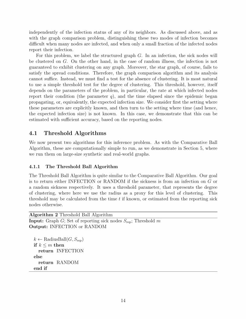
4.1.1 The Threshold Ball Algorithm

The Threshold Ball Algorithm is quite similar to the Comparative Ball Algorithm. Our goalis to return either INFECTION or RANDOM if the sickness is from an infection on G ora random sickness respectively. It uses a threshold parameter, that represents the degreeof clustering, where here we use the radius as a proxy for this level of clustering. Thisthreshold may be calculated from the time t if known, or estimated from the reporting sicknodes otherwise.

Algorithm 2 Threshold Ball Algorithm

Input: Graph G; Set of reporting sick nodes Srep; Threshold mOutput: INFECTION or RANDOM

k ← RadiusBall(G,Srep)if k ≤ m then

return INFECTIONelse

return RANDOMend if

14

4.1.2 The Threshold Tree Algorithm

The Threshold Tree Algorithm is similar, but rather than use ball-radius as a proxy for degreeof clustering, it uses the weight of a minimum-weight spanning tree connecting all reportinginfected nodes. We denote the weight of this tree on graph G for set S as SizeTree(G, S).This algorithm also requires a threshold parameter. As before, the appropriate thresholdmay be calculated using the time t, or estimated from the set of reporting sick nodes.

Algorithm 3 Threshold Tree Algorithm

Input: Graph G; Set of reporting sick nodes Srep; Threshold mOutput: INFECTION or RANDOM

k ← SizeTree(G,Srep)if k ≤ m then

return INFECTIONelse

return RANDOMend if

4.2 Summary of Results

We analyze this inference problem and in particular the performance of our two algorithms,the Threshold Ball Algorithm and the Threshold Tree Algorithm, on three types of graphs.First, we consider an infection on a d-dimensional grid. In this case, both our algorithms areable to (asymptotically) eliminate Type I and Type II error, for up to a constant fraction ofsick nodes, even when only a logarithmic fraction report sick. Orderwise, it is clear that thisis the best any algorithm (regardless of computational complexity) can hope to achieve. Ourempirical results verify this performance, and also show that the Ball Algorithm outperformsthe Tree Algorithm on the grid.

Next we consider tree graphs. Here we show that the Tree Algorithm can correctlydiscriminate between infections and random sickness for larger numbers of reporting sicknodes than the Ball Algorithm is able to handle. Finally, we analyze Erdos-Renyi graphsunder two different connectivity regimes: a low-connectivity with edge probability close tothe regime when the giant component emerges; and a high connectivity regime the producesdensely connected graphs. Again, we show that each algorithm can identify an infection withprobabilities of error that decay to 0 as the network size goes to infinity, for appropriateranges of parameters. Not surprisingly, the more densely connected, the more difficult itbecomes to obtain a good measure of ‘clustering.’ Consequently, in these latter regimes, wefind that one needs to intercept the sickness much earlier, i.e., with many fewer reportingsick nodes, in order to hope to accurately discriminate between the two potential sicknessmechanisms. In the Erdos-Renyi setting, we are unable to find direct analytic results tocompare our two algorithms. However, in Section 5 we evaluate them empirically and findthat the Ball Algorithm tends to perform better, despite its relative algorithmic simplicity.

15

4.3 Multidimensional Grids

Let G(n) be a n-node d-dimensional grid network, with side length n1/d. As before, to avoidedge effects, we let the opposite edges of the grid connect, so that the graph forms a torus,thereby eliminating any dependence of our results on the initial source of an infection. In thissection, we show that both the Threshold Ball Algorithm and the Threshold Tree Algorithmcan successfully distinguish an epidemic from a random illness, even when many nodes areinfected, yet very few report the infection.

We consider first the Threshold Ball Algorithm. The key result here is the Shape Theoremgiven in Lemma 1, which, recall, essentially says that with high probability, the shape of theset of infected nodes closely resembles a ball. The key quantity, then, is the radius of thisball, i.e., the threshold the algorithm chooses in order to decide if the underlying cause ofthe illness is a spreading epidemic, or a random illness.

Like before, we denote the set of reporting nodes Srep(n). We first assume that in additionto the reporting likelihood, q, we know the time t(n) that has elapsed since the first infection(or, equivalently, the expected size of the infection). The threshold the algorithm uses isthen a simple (linear) function of t(n). We then give an adaptive algorithm, that estimatest(n) and hence the optimal threshold to use, from the number of infected nodes reporting,and the reporting likelihood. We omit the superscript n when it is clear from context.

The next result says that as long as the number of reporting sick nodes is at least log n,then even if a constant fraction of nodes are infected, the Threshold Ball Algorithm cansuccessfully distinguish the cause of the illness, provided that the time t is known. We notethat this requirement on the number of reporting sick nodes is essentially tight, i.e., theresult cannot be improved orderwise. We also note that this requirement on the numberof reporting nodes, along with the time t, implicitly constrains the underlying parametersof the problem setup, namely q. We also prove the algorithm succeeds under similar (butslightly more restrictive) conditions when t is not known. We use µ to denote the expectedrate that an infection travels along an axis on the grid. As remarked above, this rate µ isonly a function of the dimension of the graph, since we assume the spreading rate to benormalized. We have the following.

Theorem 4.1. Consider the Threshold Ball Algorithm (Algorithm 2). Suppose that theexpected number of reporting nodes scales at least as log n.

(a) Suppose t is known. Set the threshold m = 1.1dµt. Then if the expected number ofinfected nodes is less than n/(4d)d,

P (error)→ 0.

(b) Next, suppose time t is unknown. Let Xrep be the number of nodes reporting an infection,card(Srep). Use threshold m = 1.1d(Xrep log log n/q)1/d. Then provided that the expectednumber of infected nodes is less than n/((4d)d log log n),

P (error)→ 0.

In other words, an infection can be identified in both cases with probability approaching1 as n tends to infinity. Note that the guarantee is identical, up to the log log n factor in

16

the denominator; this is the price we pay for not explicitly knowing the initial time of theinfection.

Proof of Theorem 4.1(a). This proof follows along similar lines as those in Section 4.3. Firstconsider the Type II error probability, the probability a spreading infection is labeled arandom sickness. This follows from the intuitive fact that an epidemic cannot spread ata rate that is a constant factor faster than µ, its expected rate of spread. Indeed, fromProposition 1,

RadiusBall(G,Srep) < 1.1dµt,

with probability tending to 1 as n→∞. This is equivalent to the Type II error probabilitytending to 0.

Now consider the Type I error probability, namely that a random sickness is mistakenfor an infection. From Proposition 2, since the number of reporting sick nodes, Srep, sat-isfy Srep > log n, the smallest ball that contains these random nodes satisfies, with highprobability,

RadiusBall(G,Srep) > n1/d/4.

Moreover, from the shape theorem of Lemma 1, we know that if the reporting sick nodeswere in fact due to an epidemic, then nearly all the nodes within the smallest ball containingthe reporting sick nodes, would in fact be sick. More precisely, Lemma 1 says that given anyradius a constant factor less than n1/d/4, with high probability, all nodes inside that ball areinfected. Thus, all nodes in a ball of radius 0.9n1/d/4 would be infected, if the true infectionmechanism were an epidemic. But this means that the total number of nodes actuallyinfected is at least the number of nodes in this ball. By assumption, the expected number ofinfected nodes does not exceed n(1/4d)d. Comparing these, we reach a contradiction. Hence,the Type I error probability also tends to 0.

We now use the previous result to prove that the adaptive threshold, where we use thenumber of reporting nodes to estimate t, also works. First we state a simple lemma tocharacterize the number of sick nodes.

Lemma 2. If at least X nodes are sick, then the number of reporting nodes is at least(1− δ)qX with probability at least 1− exp(−(1− δ)2qX/2).

Proof. This is a well known Chernoff bound.

Theorem 4.1(b) follows from this in a simple manner.

Proof of Theorem 4.1(b). Let Xrep be the number of reporting sick nodes, and let X =Xrep/q (that is, X is basically the expected number of sick nodes based on the numberreporting). From the previous lemma, we have

P (X log log n < card(S))→ 0.

Let µ be the asymptotic rate at which an infection travels, as before. Let ε > 0. From theproof of Theorem 4.1(a), at time t, we know for δ > 0

P (card(S) < 2(1− ε)(µt)d)→ 0.

17

Hence t < (X log logn)1/d

µ(2(1−ε))1/d with high probability. Naturally, increasing t only increases the

infection size, so it is only necessary to consider the maximum likely t. In particular, if the

threshold m = µtmax = µ(X log logn)1/d

µ(2(1−ε))1/d , then from Theorem 4.1(a), the adaptive thresholding

algorithm has Type I error probability approaching 0. In addition, if X is ω(log n), the TypeII error probability decays to 0 as well, from the same theorem.

4.4 Trees

We consider the problem on tree graphs. Unlike graphs (and more generally, geometricgraphs), trees have exponential spreading rates, and hence manifest fundamentally differentbehavior. Indeed, while simple, tree graphs convey the key conceptual point of this section:the difficulty of distinguishing an epidemic from a random sickness on graphs where theinfection spreads quickly. In addition, while the results do not immediately carry over, thebehavior on a tree provides an intuition for the behavior of an infection on an Erdos-Renyigraph, which we cover in the next section.

Thus, let G(n) be a balanced tree with n nodes, constant branching ratio c ≥ 2, anda single root node. In the case of an infection, instead of choosing a node at random tobe the original source of the infection, we always choose the root of the tree. This is themost interesting case, since otherwise a constant fraction of the nodes are very far from theinfection source and bottlenecked by the root node. Also, this precisely models the scenariofor locally tree-like graphs, such as Erdos-Renyi graphs. We again omit the indexing on nwhen it is clear by context.

First we examine the performance of the Threshold Ball Algorithm on this graph. Againrecall the meaning of t: it is the time at which the sicknesses are reported, and also a proxyfor the expected number of infected nodes.

Theorem 4.2. Suppose the Threshold Ball Algorithm (Algorithm 2) is used. Additionally,suppose t is sufficiently large that the expected number of reporting nodes is at least log n.

(a) In the case t is known, there exist constants b, β such that if the expected number ofinfected nodes is less than nβ, then the tree algorithm with threshold m = 1.1bt succeeds:

P (error)→ 0.

(b) On the other hand, suppose t is not known. Define Xrep as card(Srep). Then there existsconstants b2 and β, with the threshold set m = 1.1b2 log(Xrep(log log n)2/q), where if theexpected number of infected nodes is less than nβ,

P (error)→ 0.

The constant β is identical is both parts (a) and (b).

Proof of Theorem 4.2(a). To prove this theorem, we prove the following more general state-ment:

For some constant β < 1, if qE[card(S)] = ω(1) and E[card(S)] < nβ, then the TypeI error probability tends to 0. Next, there exists a constant b such that if b0 > b and the

18

threshold m > b0t for all n, then the Type II error probability converges to 0 asymptotically,as the tree size scales.

The Type II error bound follows from results in first passage percolation [15]. In particu-lar, one can compute the fastest-sustainable transit rate. This quantity is basically the timefrom the root to the leaves, normalized for depth, as the size of the tree scales. Formally(again, see [15] for details), let us consider a limiting process of trees whose size grows toinfinity, with Γn denoting the balanced tree on n nodes, and δ(Γn) denoting the set of pathsfrom the root to the leaves, and for a node v ∈ p for some path p ∈ δ(Γn), let Tv denotethe time it takes the infection to reach node v. Then the fastest-sustainable transit rate isdefined as:

limn

infp∈δ(Γn)

lim supv∈p

Tvdepth(v)

.

Basic results [15] show that this quantity exists and is finite, and thus shows that the rate atwhich an infection travels, defined as the maximum distance of the infection from the rootover time, converges to a constant b that depends on the branching ratio. The probabilitythat an infection travels at a faster rate converges to 0 in the size of the tree. This establishesthe Type II result.

The Type I error result follows simply as well. Given the branching ratio, c, there arecm+1−1c−1

nodes within a distance m from the root. Again letting Srep denote the number

of reporting sick nodes, the probability of a Type I error is controlled by ( cm

n)Srep – the

probability that the randomly sick nodes are closer than the threshold m to the root. Thenif cm is o(n), it is sufficient that the probability that Srep = 0 goes to 0. This occurs if theexpected number of reporting sick nodes is ω(1). That is, we need qE[card(S)] = qe(c−1)t =ω(1), calculating E[card(S)] with a simple differential equation. Alternatively, if cm = αnfor some constant α < 1, then we require Srep to increase with n with probability 1. Thesame condition as before is sufficient for this to be true. This completes the Type I result.

Using both these results, there is a choice of m such that both error types become rare aslong as cb0t < αn, so ct < (αn)1/b0 . The theorem follows using a particular threshold.

Proof of Theorem 4.2(b). First, note that E[card(S)] scales as e(c−1)t. In fact, for any fixedε > 0, card(S) > e(c−1)t/(1+ε) with probability approaching 1 (for example, see [18]). Now wecan proceed as in the proof of Theorem 4.1(b).

As before, let Xrep be the number of reporting sick nodes, and X = Xrep/q. Then weconclude tmax = (1 + ε)/(c−1) log(X(log log n)2). Hence, by setting b2 = (1 + ε)b/(c−1), wesee the Type II error probability converges to 0 by Theorem 4.2(a). Using the same theorem,we see the Type I error also goes to 0.

Thus, the Threshold Ball Algorithm succeeds until the farthest infected node reaches theedge of the graph. At this point, the ball radius can increase no further, thus there is nohope of distinguishing an infection from a random sickness. Since this farthest point travelsat a faster rate than the bulk of the infection, the Ball Algorithm can only work up to sometime logc n/b. The Threshold Tree Algorithm, however, is better suited for this setting. Weconsider this next, and show that the Tree Algorithm can still correctly identify an infectionwith high probability nearly to the point where Θ(n) nodes are sick. This includes infectiontimes close to logc n, the time it takes for every node to be infected. From this, we see that

19

the Tree Algorithm works for a wider range of times compared to the Ball Algorithm. Thisis also demonstrated by simulations in Section 5.

We note that the threshold in the results below on the Tree Algorithm, depend onE[card(S)] instead of depending explicitly on t, but as discussed previously, these are es-sentially equivalent, and we switch between the two merely to simplify notation and theexposition.

Theorem 4.3. Consider when the Threshold Tree Algorithm (Algorithm 3) is applied to thisproblem. Suppose q > log log n/ log n, and t is sufficiently large that the expected number ofreporting nodes is at least log n.

(a) Consider when t is known. Then for any constant α < 1, if the expected number ofinfected nodes scales as less than nα, with threshold m = E[card(S)] log log n,

P (error)→ 0.

(b) Suppose t is not known. Set Xrep = card(Srep), the number of nodes reporting an infec-tion. Use threshold m = Xrep/q(log log n)3. Then if for any constant α < 1, the expectednumber of infected nodes is less than nα,

P (error)→ 0.

Proof of Theorem 4.3(a). We prove the following generalization of the theorem: The Type Ierror probability converges to 0 for any choice of the threshold m = o(qE[card(S)] log n) withqE[card(S)] = O(nα) for some α < 1. In addition, the Type II error probability convergesto 0 if m = ω(E[card(S)]).

First we prove the Type II error result (mistaking an infection for a random sickness).Since the Steiner tree containing the reporting nodes can be no larger than the infectionitself, the Type II error converges to 0 as long as we use a threshold m = ω(E[card(S)]) fromMarkov’s inequality. Next, we evaluate the Type I error probability (mistaking a randomsickness for an infection). This requires estimating the size of the Steiner tree containingthe reporting sick nodes. By assumption, the number of reporting sick nodes increases withn, the probability that there are sick nodes on at least two subtrees of the root node goesto 1, hence the root of the tree is in the Steiner tree connecting the randomly sick nodeswith high probability. Given this, we see that a node is in the Steiner tree if and only if itis infected or a node below it in the tree is infected. By assumption, E[card(Srep)] > log n.Let Xrep = card(Srep), and hence Xrep is ω(1). Choose the first level in the tree that has atleast Xrep/c nodes. Then there are between Xrep/c and Xrep subtrees below that level. Itis straightforward to show that each sick node in the tree has at least a 1/2 probability ofbeing a leaf node since c ≥ 2. Since at least Xrep nodes are sick, at least Xrep/4 of the leafnodes are sick and distributed independently among the at most Xrep subtrees. Therefore,the total number of subtrees with sick nodes at the bottom is at least Xrep/(8c). In addition,each leaf node in a separate subtree requires a path at least up to the aforementioned levelin the Steiner tree. This gives us the following high probability bound on the Steiner tree

20

size.

SizeTree(Srep) >Xrep

8c(logc n− logcXrep)

> Xrep(1− α) logc n

8c.

For any w = o(E[Xrep]), we know that Xrep > w with probability approaching 1 sincethe number of sick nodes in a random sickness is highly concentrated. Therefore, if m =o(E[Xrep] logc n), which is equivalent to m = o(qE[card(S)] log n), the Type I error proba-bility tends to 0.

Proof of Theorem 4.3(b). Let Xrep = card(Srep). Let X = Xrep/q, roughly the expectednumber of total sick nodes. Then X log log n upper bounds card(S) with high probabilityas shown previously. In addition, like before, card(S) log log n > E[card(S)] with proba-bility approached 1. Then from Theorem 4.3(a) with m = X(log log n)3, we see that bothprobability of errors decrease to 0 asymptotically.

4.5 Erdos-Renyi Graphs

In this section, we consider Erdos-Renyi graphs. A notable difference in the topology ofErdos-Renyi graphs and grids is that the diameter of the former scales much more slowly(logarithmically) with graph size. That is, Erdos-Renyi graphs are more highly connected,in the sense that no two nodes are too far apart. This makes distinguishing an infectionfrom a random sickness more difficult on these graphs.

We consider two connectivity regimes: the regime where the giant component firstemerges, and each node has a constant expected number of edges, and then a much morehighly connected regime, where the graph demonstrates different local properties, and dis-crimination between random sickness and infection is harder still.

4.5.1 Detection with Constant Average Degree

We first consider Erdos-Renyi graphs with constant average degree. Define the graphG(n) = G(n, p) to be the graph with n nodes, where for each pair of nodes, there is anedge between them with probability p. In the section above, we use c to denote the branch-ing ratio. We overload notation and use it again to measure the spread of the graph, buthere as the expected degree: let p = c/n with c > 1. In this regime, the graph is almostsurely disconnected, but there is a giant component. Since this problem would be trivialon a disconnected graph, we limit both the infection and random sick nodes to the giantcomponent. We show that unlike the case of trees, our algorithms are unable to distinguishinfection from random sickness when nearly a constant fraction of nodes are infected. In-stead, we consider infections that cover only o(n) nodes. As is well-known (e.g., [16]) in thisconnectivity regime, the graph is locally tree-like, and hence tree-like in the infected region.This allows us to leverage some results from the previous section, although direct translationis not possible, particularly in the analysis of our second algorithm. We will drop the indexon n for clarity.

21

Again we note that in the next two theorems, the threshold depends on t and E[card(S)],respectively. As discussed, these are essentially equivalent, and the choice amounts to easeof notation and exposition.

Theorem 4.4. Suppose we use the Threshold Ball Algorithm (Algorithm 2). Consider thecase when the expected number of reporting nodes is no less than log n.

(a) Suppose we have knowledge of t. There are constants b, β where, using threshold m = btand with expected number of infected nodes less than nβ,

P (error)→ 0.

(b) Consider unknown t. We set Xrep to be the number of nodes reporting an infection,card(Srep). Then there exists constants b2 and β such that for threshold m = b2 log(Xrep/q(log log n)2)and if the expected number of infected nodes is less nβ,

P (error)→ 0.

The constant β is the same for both (a) and (b).

Proof of Theorem 4.4(a). Consider the Type II error probability. In this case, from Propo-sition 3, there is a constant b such that, with probability converging to 1,

RadiusBall(G,Srep) < bt = m.

Therefore, the Type II error probability tends to 0.Now we bound the Type I error probability. From Proposition 4, with probability tending

to 1,

RadiusBall(G,Srep) >log n

3 log c.

Therefore, it is sufficient to show m < logn3 log c

. Since the infection size is o(n), we use a

branching process approximation to find that for some λ, E[card(S)] → eλt. Define β =λ/(3b log c). Since E[card(S)] < nβ by hypothesis,

λt < β log n.

With some computation, m = bt < log n/(3 log c). Hence, the Type I error probability alsodecays to 0.

Proof of Theorem 4.4(b). As is shown above, E[card(S)] scales asymptotically as eλt forsome constant λ. In particular, for abitrary constant ε > 0, E[card(S)] > eλt/(1+ε) withprobability approaching 1. Then let Xrep be the number of reporting sick nodes and letX = Xrep/q, so X log log n > card(S) with probability tending to 1 as shown previously.From this, we conclude tmax = (1 + ε)/λ log(Xrep/q(log log n)2). Then by Theorem 4.2(a),with b2 = (1 + ε)b/λ and m = b2 log(Xrep/q(log log n)2), we see that the Type II errorprobability converges to 0. From the same theorem, the Type I error goes to 0 as well.

22

The Tree Algorithm is more complex to analyze for this graph. The more delicate analysiscomes from the challenge of bounding the size of the Steiner tree for the random sicknessprocess, needed to control Type I error.

Theorem 4.5. Suppose the Threshold Tree Algorithm (Algorithm 3) is applied to this prob-lem. Assume that the expected number of reporting nodes is at least log n and q is constant.

(a) Consider the case where t is known. Let the threshold m = E[card(S)] log log n. For anyα < 1/2, if the expected number of infected nodes scales as less than nα,

P (error)→ 0.

(b) Suppose we have unknown t. Define Xrep as card(Srep). In this case, set the threshold tobe m = (Xrep/q)(log log n)3. Then like before, for any constant α < 1/2, if the expectednumber of infected nodes is less than nα,

P (error)→ 0.

Proof of Theorem 4.5(a). We show the following more general statement: The Type II errorprobability decays to 0 if the threshold is chosen as m = ω(E[card(S)]) and E[card(S)] =o(n). The Type I error probability goes to 0 when m < kqE[card(S)] for some constantk = o(log(n/(qE[card(S)])2)) and qE[card(S)] = o(

√n).

First, if the sickness is from an infection, the smallest tree connecting the reporting sicknodes must have size no more than the actual number of sick nodes. Hence, to boundthe Type II error, it is sufficient to bound the probability the number of infected nodesis over a certain size. This probability decreases to 0 as long as m is ω(E[card(S)]) whenE[card(S)] = o(n). To see this, recall that in this regime, the graph looks locally tree-like.Consequently, we can bound the maximum number of infected nodes using bounds on thedistance an infection can travel (e.g., see [15]). Again, Markov’s inequality provides the exacterror bound in the theorem statement.

To control Type I error probability, that a random sickness is mistaken for an infection,we must lower bound the size of the Steiner tree of a random sickness. For v ∈ Srep, letdv denote the distance from that node to the nearest other sick node. First we show that∑

v∈Srepdv ≤ 2SizeTree(G,Srep). Note that the bound is attained for some graphs, such as a

star graph with the central node uninfected.Consider the Steiner tree subgraph, and duplicate all edges on it. Since the degree of

each node in the subgraph is even, there is a cycle that connects all these nodes. Naturally,the length of this cycle, which is twice the size of the Steiner tree, is larger than the lengthof the smallest cycle connecting all sick nodes. In addition, the length of this cycle is at least∑

v∈Srepdv, since the distance from one sick node to the next sick node in the cycle is clearly

no smaller than the distance from that sick node to the closest sick node. This establishesthat

∑v∈Srep

dv ≤ 2SizeTree(G,Srep).Now we simply need to bound dv. To do this, we need an understanding of the neighbor-

hood sizes in a G(n, p) graph. But as the size of the graph scales, this is also straightforwardto do: recalling that the probability of an edge is c/n and hence the expected degree of eachnode is (asymptotically) c, then for typical nodes and arbitrary constant ε > 0, there are

23

no more than ((1 + ε)c)d nodes within distance d provided that d = ω(1), using a branchingprocess approximation.

Let Xrep be the number of reporting sick nodes. Now assume Xrep = o(√n). Let ε > 0

and l = εn/X2rep. Let k = o(log(n/X2

rep)). Using the above distance distribution calculation,we find that each sick node v, there are less than l nodes within distance k. As the sicknodes are randomly selected, the probability that none of these are within a distance k fromv is bounded by (1−Xrep/n)l → e−ε/Xrep → 1− ε/Xrep. Thus the distance to the closest sicknode to v is at least k, i.e., dv > k, with high probability, and using a simple union bound,the same is true, simultaneously, for all sick nodes. Hence the Steiner tree joining the set ofreporting sick nodes is of size at least SizeTree(G,Srep) ≥ (1/2)

∑dv = (1/2)kqE[card(S)],

with probability decaying to zero. Therefore, the Type I error probability tends to 0 as longas the threshold satisfies m < kqE[card(S)]/2, for k = o(log(n/(qE[card(S)])2)). Using thisresult, we find that the Tree Algorithm can succeed so long as q log(n/(qE[T ])2) = ω(1).This is a complex condition, though the conditions given in the theorem are sufficient for itto be true.

Proof of Theorem 4.5(b). As in previous sections, we let Xrep be the number of reportingsick nodes, and define X = Xrep/q. Then as in Theorem 4.5(a), X log log n upper boundscard(S) and card(S) log log n > E[card(S)] with probability approaching 1. Then fromTheorem 4.5(a), we see that for the specified threshold, both probability of errors decreaseto 0 asymptotically.

4.5.2 Detection on Dense Graphs

Now we consider the case of an Erdos-Renyi graph with a denser set of edges. Higher con-nectivity means the infection spreads faster, making it more difficult to distinguish betweenspreading mechanisms. The performance depends critically on the exact scaling regime. Weconsider the regime where there exists d ∈ Z and constants ε, h ∈ R such that ε < nd−1pd < hholds for all n as n→∞. This connectivity regime has been studied in various places – see,for example, [19] for further discussion of this scaling regime and properties of these densegraphs. The next result bounds the size of the Steiner tree on a random collection of nodes,and is the key result for bounding the Type I error.

Lemma 3. Suppose nodes become sick, independently of each other, with probability n1/d/n,so that the expected number of reporting sick nodes is qn1/d. Further suppose G = G(n, p)whose parameters satisfy ε < limn→∞ n

d−1pd < h for d > 4. Let Z be the size of the minimumSteiner tree connecting the reporting sick nodes. Also, let m < (d−3)qn1/d/2 be the thresholdfor the Steiner tree size in the Tree Algorithm. Then Z satisfies the following probabilisticlimit: limn→∞ Pr(Z < m) = 0.

Proof. Using precisely the same argument as above, we can lower-bound the size of theSteiner tree by

∑dv ≤ 2Z, where the sum is over all reporting sick nodes, and as before, dv

denotes the minimum distance from a reporting sick node v to the nearest other reportingsick node. To lower bound the size of this sum, we rely on a result from [19] that showsthat in this scaling regime, the asymptotic distribution of the distance between two randomnodes is positive on only d and d + 1. That is, almost all nodes are either at distance d or

24

d+ 1 from any given node v, and thus the distance distribution concentrates sharply aroundd. To put this another way, let Fd be the probability that a random node is at distance morethan d from A. Then for any d > 1, if nd−1pd < h, we have

limFd = limn→∞

exp−nd−1pd .

Recall limn→∞ nd−1pd is bounded between ε and h.

Now we condition on the number of sick nodes, card(S). Using the same definite asbefore, let Xrep be the random variable with Xrep = card(Srep). Note E[card(S)] = n1/d andthe expected number of reporting sick nodes E[Xrep] = qE[card(S)]. We can compute the

probability that the closest sick node is at distance more than d from a sick node v simply

as FXrep

d→ exp−(Xrep/n)(np)d . Using our scaling regime, we know that (εn)1/d < np < (hn)1/d.

To simplify notation, let h′ = h1/d. We have

FXrep

d−3 → 1−Xrep/n(np)d−3

> 1−Xrep/h′nn(d−3)/d.

Using a simple union bound, we find that the probability that some reporting sick nodeis within distance d − 3 of another reporting sick node is at most X2

rep/h′nn(d−3)/d. Since

Xrep is a binomial random variable (since we condition on card(S)), it concentrates aboutits mean: for any ε′ > 0, Pr((1 − ε′)E[Xrep] < Xrep < (1 + ε′)E[Xrep]) → 1. When Xrep

is within this range, we find that∑dv > (d − 3)(1 − ε′)E[Xrep] with probability at least

1− (1 + ε′)2h′E[Xrep]2n−3/d > 1−Cn−1/d for some constant C. This converges to 1 for largeenough n. Thus, we have shown the desired result.

Now the probability of error calculations and hence the proof of correctness for the TreeAlgorithm follows directly from the above.

Theorem 4.6. For graph G as above, suppose the expected number of reporting sick nodes isqn1/d and t is known. Then for the Threshold Tree Algorithm, the probability of a Type I errorconverges to 0, as long as the threshold satisfies m < (d−3)qn1/d/2. The probability of a TypeII error upper bounded by 2/(d−3−ε) as long as the threshold satisfies m > (d−3−ε)qn1/d/2,for any value of ε > 0 such that ε+ 3 < d. This bound converges to 0 as d→∞.

Proof. Consider first the probability of a Type I error. This is the probability that a randomsickness has a Steiner tree of size less than m. From Theorem 3, this probability convergesto 0 if E[card(S)] = O(n1/d).

Second, consider the probability of a Type II error. As we have argued before, the sizeof this tree is no more than the total number of infected nodes, so it is sufficient to findthe probability there are more than m infected nodes. The Type II error probability boundfollows from using Markov’s Inequality.

5 Simulations

The above sections give theoretical guarantees for the correctness of our algorithms, andthus characterize their ability to distinguish the cause of an illness – be it detecting one

25

graph versus another as the causative network, or the determination that a sickness is anepidemic or a random illness. In this section, we explore these questions empirically. Wevalidate our theoretical analysis on graphs that are generated from the ensembles we addressin our theorems (grids, random graphs, trees) and then also consider epidemics on real-worldgraphs, and demonstrate that on these topologies as well, our algorithms perform well.

5.1 Graph Comparison

We simulated the performance of the Comparative Ball Algorithm to evaluate the perfor-mance empirically. We determined the error rate over a range of t for several pairs ofgraphs. We evaluated the two different standard graph topologies considered earlier, gridsand Erdos-Renyi graphs.

We simulated the infections on various pairs of the graphs over a range of times. In orderto portray the results in a comparable way, we plotted the error rate versus the averageinfection size instead of time. This is necessary because different times result in very differentinfection sizes for the different graphs. That is, the infection is large even at low t on anErdos-Renyi graph, and vice versa for a grid graph. This would introduce a misleading effectin the results.

Each node in the graphs received a random label to ensure independence. We use n =1, 600 for each graph with q = 0.25. For the Erdos-Renyi graphs, we use p = 2/1, 600. Theprobability of error was computed over 10, 000 trials. There are two possible types of errorsin each simulation, when the infection spreads on the first graph, and when it spreads on thesecond. We label the error event ‘T:G1; A:G2’ for the error where the infection in fact travelson graph G1 (True event), but the algorithm incorrectly labels it as occurring on graph G2

(Algorithm output).The results of these simulations are shown in Figure 1. Note that up to about 5% of

the network reporting an infection, the error rates are low in all cases. The error ratesare consistently low for the ‘T:Grid1;A:Grid2’ comparison up to the point where the wholenetwork is infected. When comparing a grid and an Erdos-Renyi graph, there is a bias tolabel it an Erdos-Renyi graph at higher times, causing the ‘T:Grid;A:G(n,p)’ error to bevery high and conversely, the ‘T:G(n,p);A:Grid’ error to be very low. This suggests thatby simply modifying the Comparative Ball Algorithm to normalize with respect to a scaledgraph diameter (where the scaling parameter would be graph dependent), we could balancethese two error probabilities, and thus result in improved performance. To illustrate, bychoosing a diameter scaling value of 1.6 for the Grid graph, the plot in Figure 2 indicatesthat one could distinguish between G(n,p) and Grid graphs for a significantly larger range.We plan to study a systematic approach for such scalings as future work.

5.2 Infection vs. Random Sickness

In this section we provide simulation-based evidence of the theoretical results for the Thresh-old Ball Algorithm and Threshold Tree Algorithm. The simulations aim to demonstrate, inparticular, two facts. First, the thresholds specified in Section 4 do actually work empirically,and as the graph size increases, the probability of both types of error decrease to zero. Inaddition, this provides insight into how quickly the probability of error decays. While our

26

Figure 1: This figure shows the error probability for the algorithm on pairs of standard graphs. Various

(conditional) error probabilities are illustrated – ‘T:’ corresponds to the true network, and ‘A:’ corresponds

to the algorithm output.

Figure 2: This figure shows the error probability for the G(n,p) vs. Grid graphs for the scaled diameter

setting (diameter of G(n,p) graph is scaled by 1.6).

results include rate estimates given as part of the proof of correctness, we have not made aneffort to optimize these in this work. Next, we seek to describe the relative performance ofeach algorithm, and show that it is as described above. Thus, we show that the ThresholdBall Algorithm outperforms the Threshold Tree Algorithm on a grid; the Threshold TreeAlgorithm performs better than the Threshold Ball Algorithm on a balanced tree; and onan Erdos-Renyi graph, the performances are similar, with the Threshold Ball Algorithm

27

performing slightly better. We accomplish this by determining the probability of error for arange infection sizes. The larger the fraction of infected nodes, the more difficult the prob-lem becomes; hence we call an algorithm superior if it works for a larger fraction of infectednodes.

We note that to perform our simulations, it was necessary to use an approximate Steinertree algorithm to perform the Threshold Tree Algorithm in a reasonable time frame. Nat-urally, since the exact problem is NP-hard, this would be required in any practical use ofthis algorithm at the moment. However, as a consequence, the empirical results may differfrom the true theoretical result that would be obtained by employing an exact algorithm.Nevertheless, approximation algorithms typically have reasonable performance and we donot expect significant deviation from the correct results. The approximation algorithm weuse is the Mehlhorn 2-approximation algorithm provided by the Goblin library [20]. Thisalgorithm is an efficient algorithm which produces a Steiner tree with no more than twicethe optimal number of edges.

Each of the points in these results represents the average of 10, 000 runs. The averageinfection size, which is used to normalize the expected infection size in a random sickness,was determined by averaging the results of 10, 000 infections. For each simulation, we usea reporting probability q = 0.25, and other parameters (n, t and m) as specified in eachsection below. Finally, the graphs are plotted with error bars at 95% confidence.

Figure 3: Empirical Type I and Type II error probability vs graph size for grid graphs. The sample size is

10, 000 and infection size scales linearly with n.

5.2.1 Error Rate Versus Graph Size

Though our theoretical results have characterized the range for which each algorithm works,naturally we wish to see empirically the error probability for each algorithm and the rate atwhich the error decreases as graph size increases. Both Type I and Type II error probabilitieswere determined for each algorithm and graph topology. For this section, we have chosentime to keep the fraction of infected nodes at a consistent scaling. In particular, t = 0.2

√n

for the grid, and t = 0.5 log(0.5n) with p = 2/n for the Erdos-Renyi graph. The exactconstants for these scalings were chosen empirically so that the probability of error waslow and the Type I and Type II errors were as balanced as possible. The thresholds m

28

Figure 4: Empirical Type I error probability vs graph size for graphs G(n, 2/n). The sample size is 10, 000

and infection size scales orderwise as√n.

were also chosen with the same scaling, according to our theoretical results. To be exact,for the grid, the Threshold Ball Algorithm used threshold m = 0.75

√n and the Threshold

Tree Algorithm used threshold m = 0.28n. For the Erdos-Renyi graphs, the ThresholdBall Algorithm used threshold m = 0.69 log(4.33n) and the Threshold Tree Algorithm usedthreshold m = 0.03

√n log n log n.

Figure 3 presents our results for grid graphs. The error probability of the Threshold BallAlgorithm on a grid is very low, while the tree algorithm performs relatively poorly. Thisis expected since the Threshold Ball Algorithm is closely aligned with the true shape of aninfection on this graph. The Threshold Tree Algorithm has a much higher error probabilitywhich decays slowly with n, in particular the Type II error.

Next, the results for Erdos-Renyi graphs are in Figure 4. Here we see again that theThreshold Ball Algorithm performs better than the Threshold Tree Algorithm, at least forlarger n, and that the error probability also seems to be decreasing faster for the ThresholdBall Algorithm as well. Though a tree more closely matches the infection shape on an Erdos-Renyi graph, it is also easier for a random sickness to mimic a small tree, especially for smallworld graphs like Erdos-Renyi graphs. This causes the Threshold Ball Algorithm to beultimately superior. The Threshold Tree Algorithm is superior for larger infection sizes onbottle necked graphs (such as trees) where the random sickness can be easily distinguished,as we see in Section 5.2.2.

5.2.2 Error Rate Versus Infection Size

Next, we examine empirically how the infection duration affects the probability of error foreach of our algorithms. As discussed above, we compare the two algorithms by the rangeof infection sizes for which they work, and accordingly, we call an algorithm superior if itmaintains a lower probability of error for a larger infection size (fraction of total infectednodes). We use thresholds that minimize the empirical overall probability of error. That is,the sickness was chosen to be either an infection or simply random with equal probability,and the threshold with minimum probability of error from the simulations was chosen.

These results are presented in Figure 5 for grids, trees, and Erdos-Renyi graphs. For

29

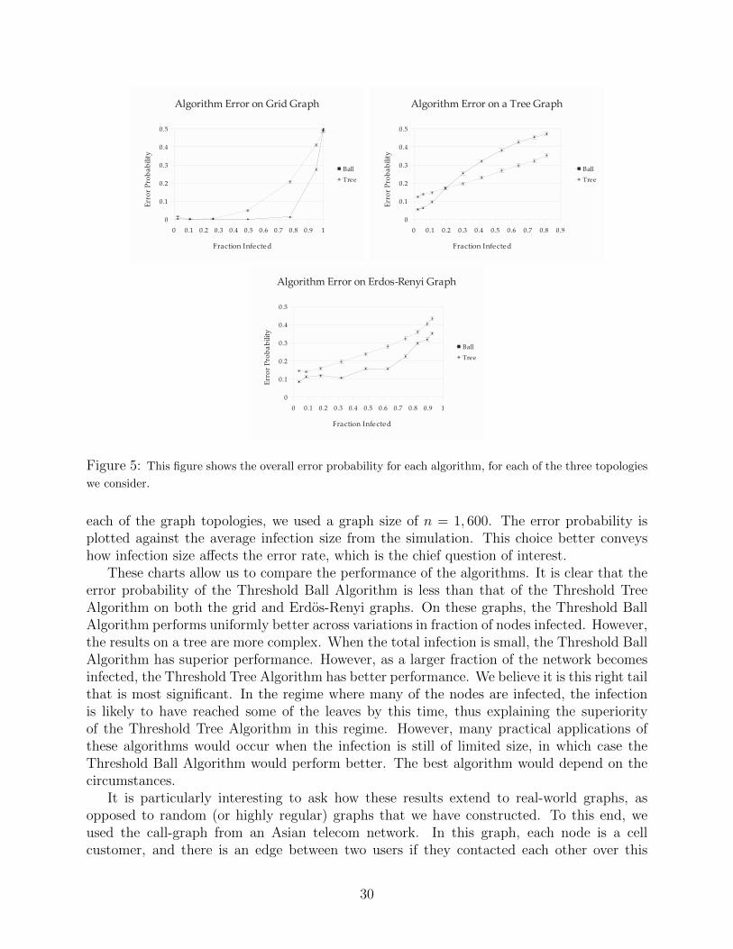
Figure 5: This figure shows the overall error probability for each algorithm, for each of the three topologies

we consider.

each of the graph topologies, we used a graph size of n = 1, 600. The error probability isplotted against the average infection size from the simulation. This choice better conveyshow infection size affects the error rate, which is the chief question of interest.

These charts allow us to compare the performance of the algorithms. It is clear that theerror probability of the Threshold Ball Algorithm is less than that of the Threshold TreeAlgorithm on both the grid and Erdos-Renyi graphs. On these graphs, the Threshold BallAlgorithm performs uniformly better across variations in fraction of nodes infected. However,the results on a tree are more complex. When the total infection is small, the Threshold BallAlgorithm has superior performance. However, as a larger fraction of the network becomesinfected, the Threshold Tree Algorithm has better performance. We believe it is this right tailthat is most significant. In the regime where many of the nodes are infected, the infectionis likely to have reached some of the leaves by this time, thus explaining the superiorityof the Threshold Tree Algorithm in this regime. However, many practical applications ofthese algorithms would occur when the infection is still of limited size, in which case theThreshold Ball Algorithm would perform better. The best algorithm would depend on thecircumstances.

It is particularly interesting to ask how these results extend to real-world graphs, asopposed to random (or highly regular) graphs that we have constructed. To this end, weused the call-graph from an Asian telecom network. In this graph, each node is a cellcustomer, and there is an edge between two users if they contacted each other over this

30

Figure 6: This figure shows the overall error probability for each algorithm on a real world graph.

network during a certain range of time. Since the original graph was too large for practicalsimulation times, we cut out a partial subset. We chose a random node and all nodes witha distance 9 and used the induced subgraph generated by these nodes. The resulting graphhas size n = 13, 189. The probability of error for a range infection sizes are presented inFigure 6. We see that the results are similar to those for a Tree graph, where the ThresholdBall Algorithm performs better on small infections, but it is out performed by the ThresholdTree Algorithm in larger infections. This is to be expected, as the intuition for the ThresholdBall Algorithm stems from the geometry of spatial grid-like networks. The call-graph hereis very much tree-like (however, with very small diameter and high degree), and infectionsare unlikely to propagate to the same depth across various leaves. This results in poor Ball“fits,” especially as the infected fraction of nodes grows. This intuition is indeed borne outin the simulations.

6 Conclusions

When an infection/virus is seen spreading over a group of people/machines, one may havemultiple possibile spreading regimes for the infection in mind, and want to know which theinfection is most likely travelling on. We considered this problem both in the case of twowell structured graphs, and in the case of comparing an infection from a random sickness.For two structured graphs, we have shown that this is possible to do with high accuracy ifthe regimes are independent and satisfy two properties: 1) An infection spreading accordingthe regime should be localized in the contact graph, and 2) A random set of nodes shouldbe spaced far apart on the graph. When these conditions are satisfied (in the sense given inthis paper), the correct spreading regime can be detected accurately with high probabilityby determining on which graph the infection appears to be more clustered. In addition,we have shown two standard types of graphs, grids and Erdos-Renyi graphs, satisfy theseproperties. In the case of comparing an infection and a random sickness, we developed twoalgorithms that solve the problem. We proved these algorithms do so with high probabilityfor grids, tree, and Erdos-Renyi graph for ranges of infection sizes dependent on the graphtopology. Our simulations here demonstrate the efficacy of our algorithms.

31

References

[1] C. Milling, C. Caramanis, S. Mannor, and S. Shakkottai, “Network forensics: randominfection vs spreading epidemic,” SIGMETRICS Perform. Eval. Rev., vol. 40, no. 1, pp.223–234, June 2012.

[2] ——, “On identifying the causative network of an epidemic,” in In Proceedings of50th Annual Allerton Conference on Communication, Control, and Computing, October2012.

[3] Wikipedia, “HIV/AIDS — Wikipedia, the free encyclopedia,” 2012, [Accessed30-Sept-2012]. [Online]. Available: http://en.wikipedia.org/wiki/HIV/AIDS

[4] J. Cohen, “Making headway under hellacious circumstances,” SCIENCE, vol. 313, pp.470–473, July 2006.

[5] A. J. Ganesh, L. Massoulie, and D. F. Towsley, “The effect of network topology on thespread of epidemics,” in INFOCOM, 2005, pp. 1455–1466.

[6] F. Ball and P. Neal, “Poisson approximation for epidemics with two levels of mixing,”The Annals of Probability, vol. 32, no. 1B, pp. 1168–1200, 2004.

[7] A. Gopalan, S. Banerjee, A. Das, and S. Shakkottai, “Random mobility and the spreadof infection,” in Proc. IEEE Infocom, 2011.

[8] N. Demiris and P. D. O’Neill, “Bayesian inference for epidemics with two levels ofmixing,” Scandinavian Journal of Stat., vol. 32, pp. 265–280, 2005.

[9] G. Streftaris and G. J. Gibson, “Statistical inference for stochatic epidemic models,” inProc. 17th International Workshop on Statistical Modeling, 2002, pp. 609–616.

[10] N. Demiris and P. D. O’Neill, “Bayesian inference for stochastic multitype epidemics instructured populations via random graphs,” Journal of the Royal Stat. Society SeriesB, vol. 67, no. 5, pp. 731–745, 2005.

[11] D. Shah and T. Zaman, “Detecting sources of computer viruses in networks: Theoryand experiment,” SIGMETRICS Perform. Eval. Rev., vol. 86, pp. 203–214, 2010.

[12] ——, “Rumors in a network: Who’s the culprit?” IEEE Transactions on InformationTheory, vol. 57, August 2011.

[13] R. Lyons and R. Pemantle, “Random walk in a random environment and first-passagepercolation on trees,” The Annals of Probability, vol. 20, no. 1, pp. 125–136, 1992.

[14] H. Kesten, “On the speed of convergence in first-passage percolation,” The Annals ofApplied Probability, vol. 3, no. 2, pp. 296–338, Nov 1993.

[15] I. Benjamini and Y. Peres, “Tree-indexed random walks on groups and first passagepercolation,” Probability Theory and Related Fields, vol. 98, pp. 91–112, 1994.

32

[16] R. Durrett, Random Graph Dynamics. Cambridge University Press, 2007.

[17] F. Chung and L. Lu, “The diameter of sparse random graphs,” Adv. in Appl. Math,vol. 26, pp. 257–279, 2001.

[18] D. R. Grey, “Asymptotic behaviour of continuous time, continuous state-space branch-ing processes,” Journal of Applied Probability, vol. 11, no. 4, pp. 669–677, December1974.

[19] V. D. Blondel, J.-L. Guillaume, J. M. Hendrickx, and R. M. Jungers, “Distance dis-tribution in random graphs and application to network exploration,” Physical Review,vol. 76, no. 066101, 2007.

[20] K. Mehlhorn, “A faster approximation algorithm for the steiner problem in graphs,”Information Processing Letters, vol. 27, pp. 125–128, 1988.

33