Embed Size (px)
Citation preview

Distressed Debt Prices and Recovery RateEstimation
Robert Jarrow
Joint Work with Xin Guo and Haizhi Lin
May 2008

Introduction
� Recent market events highlight the importance ofunderstanding credit risk.
� Credit risk pricing and hedging involves understanding:1. interest rates (stochastic discounting),2. default process (when payments stop), and3. recovery rate process (what happens after default).
� Points 1 and 2 well-studied.� Point 3, less so...

Introduction
Three sources of knowledge on recovery rates.
1. Industry papers:estimate recovery rates (not transparent, not validated by
academic community), andstudy their properties (correlation with business cycle,
dependence on �rm characteristics, ...)
2. Academic papers - use industry generated recovery rates tostudy their properties.
3. Academic papers - use pre-default debt and CDS prices toimplicitly estimate recovery rates.

Introduction
Potential problems with existing knowledge.
� Are we sure recovery rates are estimated correctly? If not,then...
� academic papers study mis-speci�ed estimates,� academic papers have no base to compare implicit estimates.

Introduction
Purposes
Primary- provide direct estimates of recovery rates usingdistressed debt prices.
Secondary - �t a model for defaulted debt prices.
(it turns out, to solve one, must also solve the other)

Introduction
Results
1. Recovery rate estimates are sensitive to the date selected forestimation (signi�cant di¤erences between using the recordeddefault date and 30 days after).
2. Prices support the belief that the market often recognizesdefault before default is recorded.
3. An extended recovery rate model provides a poor �t todistressed debt prices after the recorded default date(extension implicit in using 30 day after to estimate recoveryrate).
4. We estimate a new recovery rate process and use it to pricedistressed debt. The model �ts market prices well.

Prologue
Structural models
� Use management�s information set.� Default can be viewed as the �rst hitting time of the �rm�s assetvalue to a liability determined barrier.
� If the �rm�s asset value follows a continuous process, the value of a�rm�s debt does not exhibit a jump at default.
� No implications for risky debt prices subsequent to default.
Reduced Form Models
� Use market�s information set.� Default modeled as the �rst jump time of a point process.� Debt prices exhibit a negative jump at default.� No implications for risky debt prices subsequent to default.

Prologue
3 0 Se p 2 0 0 4 2 7 F e b 2 0 0 5 2 7 J u l 2 0 0 5 2 4 De c 2 0 0 51 0
1 5
2 0
2 5
3 0
3 5
4 0
4 5
5 0
5 5s e ri e s 1
Figure: Delta Airlines. Bankruptcy on September 14, 2005.
Consistent with the standard structural model.30-day di¤erent from default date.

Prologue
0 3 Oc t2 0 0 4 3 0 No v 2 0 0 4 2 7 J a n 2 0 0 5 2 6 M a r2 0 0 54 0
5 0
6 0
7 0
8 0
9 0
1 0 0s e ri e s 1
Figure: Trico Marine Service Inc. Bankruptcy on December 18, 2004.
Inconsistent with the structural model.(market recognized default earlier?)
30-day approximately same as default date.

Prologue
29 Se p 2004 26 Fe b 2005 26 J u l 2 00 5 23 De c 200540
50
60
70
80
90
1 00s e rie s 1
Figure: Winn Dixie Stores. Bankruptcy on February 21, 2005.
Consistent with the standard reduced form model.30-day di¤erent from default date.

Prologue
0 3 Ap r2 0 0 5 3 0 J u n 2 0 0 5 2 6 Se p 2 0 0 5 2 3 De c 2 0 0 52 0
3 0
4 0
5 0
6 0
7 0
8 0
9 0s e rie s 1
Figure: Northwest Airlines. Bankruptcy on September 14, 2005.
Partially consistent with both the reduced form and structural.30-day di¤erent from default date.
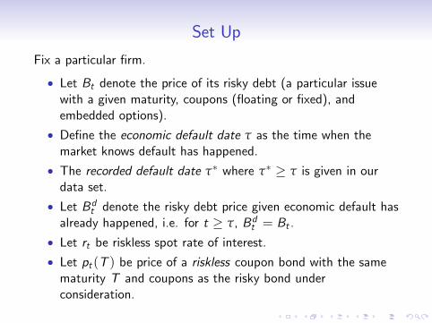
Set Up
Fix a particular �rm.
� Let Bt denote the price of its risky debt (a particular issuewith a given maturity, coupons (�oating or �xed), andembedded options).
� De�ne the economic default date τ as the time when themarket knows default has happened.
� The recorded default date τ� where τ� � τ is given in ourdata set.
� Let Bdt denote the risky debt price given economic default hasalready happened, i.e. for t � τ, Bdt = Bt .
� Let rt be riskless spot rate of interest.� Let pt (T ) be price of a riskless coupon bond with the samematurity T and coupons as the risky bond underconsideration.

Cross-Sectional Models
1. Recovery of Face Value (RFV):
Bdτ = δτF
where F is the face value of the debt (normalized to $100)2. Recovery of Treasury (RT):
Bdτ = δτpτ(T )
3. Recovery of Market Value (RMV):
Bdτ = δτBτ�

Cross-Sectional Models
� Purpose of these models is to provide the necessary inputs toprice risky debt and credit derivatives prior to default.
� Recovery rate estimation procedure is:� �x a defaulted company� �x a date τ to observe debt prices, then� estimate the recovery rate.
� Single point estimate of the recovery rate per company. Lookcross-sectionally across companies to obtain estimate.
� For example, Moody�s uses "30-day" post-default date for τ.

Data
� December 2000 to October 2007.� Debt Price Data - Advantage Data Corporation - Trade dataand broker quotes to get end of day prices 4:45 p.m.
� Filter data:� have 50 prices over a 60 day window surrounding recordeddefault date.
� Remove bond issues with missing data on maturity, coupons.� This leaves 96 issues remaining for recovery rate estimation.
� Filters imply that all our defaulted debt issues eventually �lefor bankruptcy (potential selection bias).
� Bond Characteristics - Mergent Fixed Income Database.Default is when a debt issue violates a bond covenant, missesa coupon or principal payment, or �les for bankruptcy. Agrace period of 30 days must usually pass before default isrecognized for a missed coupon.

Data - Bankruptcy Time Analysis
To get a sense for duration of distressed debt market, consideringonly issues that �le for bankruptcy.
N = 1902 Mean Std. Dev. Median N λ
Chapter 7 433.22 353.20 433 9 0.80Chapter 11 454.34 427.08 354 631 0.84
Time in Bankruptcy in Daysλ is average time spent in bankruptcy in years.

Cross-sectional Recovery Rates (RFV)
Di¤erence Count Avg. Price Std. Dev. Avg. Ratio-30 23 62.19 33.04 1.3199-20 58 48.99 28.06 1.3510-10 27 66.74 28.60 1.2382-5 51 40.42 25.81 1.2114-2 41 44.60 29.99 1.0541-1 61 45.05 29.55 0.97960 70 48.17 29.39 11 71 45.48 28.67 1.02922 63 41.27 28.85 1.02845 44 48.32 31.48 1.034110 45 54.62 28.83 1.093320 46 53.86 32.44 1.147330 64 42.31 29.30 1.0779
RFV at recorded default 48.17 statistically di¤erent from RFV at 30 day42.31.

Cross-sectional Recovery Rates (RT)
N = 96 RT EstimatesMean 0.4062Median 0.3452
Standard Deviation 0.2528First Quartile 0.1692Third Quartile 0.6374
Lower than the RFV estimates because otherwise identical defaultfree bonds trade at a premium (> $100).
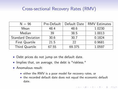
Cross-sectional Recovery Rates (RMV)
N = 96 Pre-Default Default Date RMV EstimatesMean 48.4 48.6 1.0230Median 39 38.5 1.0013
Standard Deviation 30.6 30.7 0.1824First Quartile 21.5 22 0.9681Third Quartile 67.55 69.375 1.0597
� Debt prices do not jump on the default date.� Implies that, on average, the debt is "riskless."� Anomalous result:
� either the RMV is a poor model for recovery rates, or� the recorded default date does not equal the economic defaultdate.

Time-Series Models
Bdt = m � δτeR t
τ rsds
where
m =
8<:F if RFV
pτ(T ) if RTBτ� if RMV .
Assumes that risky debt position is sold at τ, and the model pricesdebt as the value of this position. Equivalently,
Bdt = Bdτ�e
R tτ� rsds for t � τ.
This form is independent of model type. Use this to:
1. Determine economic default date.
2. Test accuracy of valuation model.

Time-Series Models - Economic Default Date
� Given our de�nition of the economic default date, using debtprices, our estimator is:
bτ = infτ��180�t�τ�
ft : Bt � Bdτ�e�R τ�t rsdsg.
� Bound below by 180 days before the recorded default date.� Our estimator depends on the information up to time τ�.

Time-Series Models - Economic Default Date
0 20 40 60 80 100 120 140 160 1800
5
10
15
20
25
Days
Cas
es
T ime Between Economic Default Date and Announced Default Date
Figure: N = 73.
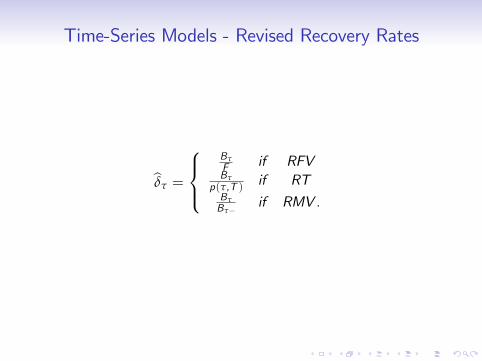
Time-Series Models - Revised Recovery Rates
bδτ =
8><>:BτF if RFVBτ
p(τ,T ) if RTBτBτ�
if RMV .
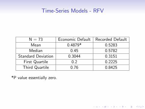
Time-Series Models - RFV
N = 73 Economic Default Recorded DefaultMean 0.4879* 0.5283Median 0.45 0.5782
Standard Deviation 0.3044 0.3151First Quartile 0.2 0.2225Third Quartile 0.76 0.8425
*P value essentially zero.
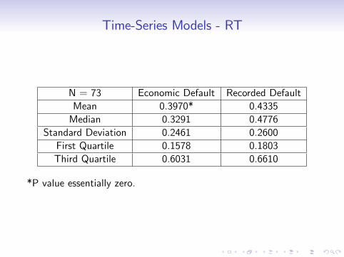
Time-Series Models - RT
N = 73 Economic Default Recorded DefaultMean 0.3970* 0.4335Median 0.3291 0.4776
Standard Deviation 0.2461 0.2600First Quartile 0.1578 0.1803Third Quartile 0.6031 0.6610
*P value essentially zero.

Time-Series Models - RMV
N = 73 Economic Default Recorded DefaultMean 0.8314* 1.0653Median 0.9094 1.0217
Standard Deviation 0.1775 0.1729First Quartile 0.7267 0.9976Third Quartile 0.9649 1.0854
*P value essentially zero.
This is consistent with a jump on the economic default date.
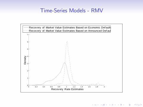
Time-Series Models - RMV
0 0.2 0.4 0.6 0.8 1 1.2 1.4 1.6 1.8 20
1
2
3
4
5
6
7
Recov ery Rate Estimates
Den
sity
Recov ery of Market Value Estimates Based on Economic Def aultsRecov ery of Market Value Estimates Based on Announced Def aults

Time-Series Models - Pricing Tests
Bdt = m � bδτeR t
τ rsds + εt for t � τ.
"Good" if the residuals have zero mean, and are i.i.d.
N = 20,942 Pricing ErrorsMean 17.81Median 9.31
Standard Deviation 28.06First Quartile 0.11Third Quartile 30.00
Very large pricing errors.
Time-Series Models - Pricing Tests
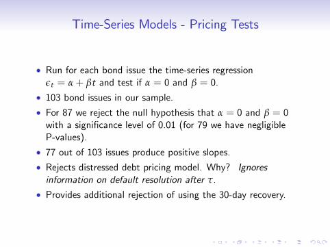
� Run for each bond issue the time-series regressionεt = α+ βt and test if α = 0 and β = 0.
� 103 bond issues in our sample.� For 87 we reject the null hypothesis that α = 0 and β = 0with a signi�cance level of 0.01 (for 79 we have negligibleP-values).
� 77 out of 103 issues produce positive slopes.� Rejects distressed debt pricing model. Why? Ignoresinformation on default resolution after τ.
� Provides additional rejection of using the 30-day recovery.

The Recovery Rate Model
� Database limitations - model the resolution of the bankruptcy�ling.
� Restrict to t � τ.
� Let τ0 represent the time to resolution of bankruptcy.
� Exponential distribution with parameter λ.
� Dollar payo¤ equal to m � δτ0 � 0 where
m =
8<:F if RFV
pτ(T ) if RTBτ� if RMV .
The Recovery Rate Model
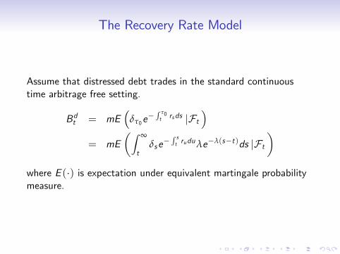
Assume that distressed debt trades in the standard continuoustime arbitrage free setting.
Bdt = mE�
δτ0e�R τ0t rsds jFt
�= mE
�Z ∞
tδse�
R st ruduλe�λ(s�t)ds jFt
�where E (�) is expectation under equivalent martingale probabilitymeasure.

The Recovery Rate Model
De�neRs � δse�
R sτ rudu
wheredRt = a(b� Rt )dt + σdWt
with a, b, σ are constants and Wt is a standard B.M. under themartingale measure.
Distressed debt price:
Bdt = meR t
τ rudu�Rt
λ
(a+ λ)+
ba(a+ λ)
�= m
�δt
λ
(a+ λ)+
ba(a+ λ)
eR t
τ rudu�

Recovery Rate Model - Estimation MethodologyEstimate λ = 0.80 using bankruptcy data.Given τ = τ�, estimate (a, b, σ, ρ) and (Rt )t�τ using KalmanFilter:
Bdtme�
R tτ rudu = At +HtRt + εt
where εt � N(0, ρ) is i.i.d. observation error.
Rt = Ct + FtRt�1 + ηt
where ηt � N(0, σ2
2a (1� 2e�a) and
At �ba
(a+ λ), Ht �
λ
(a+ λ), Ct � b(1� e�a), Ft � e�a
Given (a, b, σ, ρ,λ) and (Rt )t�τ, estimate
τ = infτ��180�t�τ�
ft : Bt � Bdτ�e�R τ�t ruduea(τ
��t)+mb(1� ea(τ��t))g
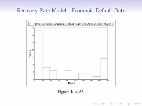
Recovery Rate Model - Economic Default Date
0 20 40 60 80 100 120 140 160 1800
5
10
15
20
25
30
35
Day s
Cas
es
Time Between Economic Def ault Date and Announced Def ault Date
Figure: N = 82.
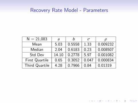
Recovery Rate Model - Parameters
N = 21,083 a b σ ρ
Mean 5.03 0.5558 1.33 0.009232Median 2.04 0.6183 0.23 0.008507Std Dev 14.10 0.2778 5.97 0.001082
First Quartile 0.65 0.3052 0.047 0.000834Third Quartile 4.28 0.7966 0.84 0.01319
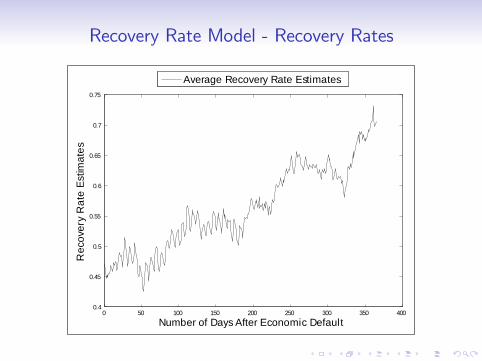
Recovery Rate Model - Recovery Rates
0 50 100 150 200 250 300 350 4000.4
0.45
0.5
0.55
0.6
0.65
0.7
0.75
Number of Days After Economic Default
Rec
over
y R
ate
Estim
ates
Average Recovery Rate Estimates

Recovery Rate Model - Recovery Rates
RFV RT RMVN = 69 EM KFM EM KFM EM KFMMean 0.4814 0.5068* 0.3919 0.4134* 0.8272 0.8868**Median 0.4006 0.55 0.3204 0.4698 0.9 0.9299StdDev 0.3029 0.2985 0.2442 0.2423 0.1780 0.125525 % 0.2 0.23 0.1578 0.1830 0.7267 0.807475 % 0.71 0.785 0.6020 0.6150 0.9577 0.9743
At economic default date.
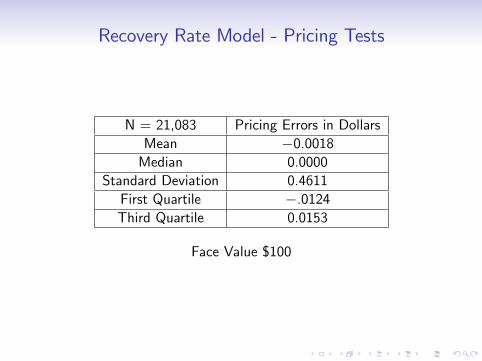
Recovery Rate Model - Pricing Tests
N = 21,083 Pricing Errors in DollarsMean �0.0018Median 0.0000
Standard Deviation 0.4611First Quartile �.0124Third Quartile 0.0153
Face Value $100

Recovery Rate Model - Pricing Tests
� Run for each bond issue the time series regressionεt = α+ βt and test if α = 0 and β = 0.
� For 83 out of 103 issues, we fail to reject the null hypothesisthat α = 0 and β = 0 with signi�cance level 0.01.
� We perform a Durbin-Watson autocorrelation test.
� For 62 out of the 103 issues, we fail to reject the nullhypothesis that corr(εt , εt�1) = 0 with signi�cance level 0.01.
� For most issues, recovery rate model �ts data well.

Epilogue
29Sep2004 09Aug2005 19Jun2006 29Apr200710
20
30
40
50
60
70
80series1
Figure: Delta Airlines

Epilogue
03Oct2004 30Nov2004 27Jan2005 26Mar200540
50
60
70
80
90
100series1
Figure: Trico Marine Service Inc.

Epilogue
30Sep2004 30Jun2005 30Mar2006 28Dec200640
50
60
70
80
90
100
110series1
Figure: Winn Dixie Stores
Epilogue
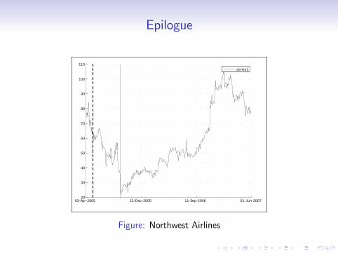
03Apr2005 22Dec2005 11Sep2006 01Jun200720
30
40
50
60
70
80
90
100
110series1
Figure: Northwest Airlines

Conclusions
� Economic default date di¤ers from reported default date.
� Recovery rate estimates based on 30 days after recordeddefault are misspeci�ed.
� Recovery rate estimates based on recorded default datesigni�cantly di¤erent from economic default date.
� Implies that:� Existing academic studies using 30 day recovery rates, resultsquantitatively incorrect, but qualitatively?
� Recovery rate estimates can be improved.� Time to economic default estimates can be improved.� Prices of credit derivatives and pre-default risky debt can beimproved.
� Exploring these implications await subsequent research.

![Distressed Debt Prices and Recovery Rate Estimation · and Das and Hanouna [10]) we formulate and estimate a new recovery rate process useful for pricing distressed debt. Our model](https://img.pdfslide.net/doc/110x75/5fab8917f3b06d36ff1e1bf5/distressed-debt-prices-and-recovery-rate-estimation-and-das-and-hanouna-10-we.jpg)