Dra

ftDynamics and control of wall-bounded shear flows

Mihailo Jovanovicwww.umn.edu/∼mihailo

Center for Turbulence Research, Stanford University; July 13, 2012

Dra

ft

M. JOVANOVIC 1

Flow control

technology: shear-stress sensors; surface-deformation actuators

application: turbulence suppression; skin-friction drag reduction

challenge: distributed controller design for complex flow dynamics

Dra

ft

M. JOVANOVIC 2

Outline¶ DYNAMICS AND CONTROL OF WALL-BOUNDED SHEAR FLOWS

• The early stages of transition

? initiated by high flow sensitivity

• Controlling the onset of turbulence

? simulation-free design for reducing sensitivity

Key issue:

high flow sensitivity

· CASE STUDIES

• Sensor-free flow control

? streamwise traveling waves

• Feedback flow control

? design of optimal estimators and controllers

¸ SUMMARY AND OUTLOOK

Dra

ft

M. JOVANOVIC 3

Transition to turbulence

• LINEAR HYDRODYNAMIC STABILITY: unstable normal modes

? successful in: Benard Convection, Taylor-Couette flow, etc.

? fails in: wall-bounded shear flows (channels, pipes, boundary layers)

• DIFFICULTY 1Inability to predict: Reynolds number for the onset of turbulence (Rec)

Experimental onset of turbulence:

{much before instabilityno sharp value for Rec

• DIFFICULTY 2Inability to predict: flow structures observed at transition

(except in carefully controlled experiments)

Dra

ft

M. JOVANOVIC 4

LINEAR STABILITY:

? For Re ≥ Rec ⇒ exp. growing normal modescorresponding e-functions

(TS-waves)

}= exp. growing flow structures

-

x���z

NOISY EXPERIMENTS: streaky boundary layers and turbulent spots

-

x6

z

Failure of classical linear stability analysis for wall-bounded shear flows

•

Classical theory assumes 2D disturbances

•

Experiments suggest transition to more complex flow is inherently 3D: streamwise streaks

Flow type Classical prediction Experiment

Plane Poiseuille 5772 ~ 1000

Plane Couette ∞ ~ 350Pipe flow ∞ ~ 2200-100000

•

Critical Reynolds number for instability

M. Matsubara and P. H. Alfredsson, J. Fluid Mech. 430 (2001) 149

Boundary layer flow with free-stream turbulence

Flow-

x6

z

Matsubara & Alfredsson, J. Fluid Mech. ’01

Dra

ft

M. JOVANOVIC 5

• FAILURE OF LINEAR HYDRODYNAMIC STABILITY

caused by high flow sensitivity

? large transient responses

? large noise amplification

? small stability margins

TO COUNTER THIS SENSITIVITY: must account for modeling imperfections

TRANSITION ≈ STABILITY + RECEPTIVITY + ROBUSTNESS

←−

←−

flowdisturbances

unmodeleddynamics

Farrell, Ioannou, Schmid, Trefethen, Henningson, Gustavsson, Reddy, Bamieh, etc.

Dra

ft

M. JOVANOVIC 6

Tools for quantifying sensitivity

• INPUT-OUTPUT ANALYSIS: spatio-temporal frequency responses

-

d

Free-stream turbulenceSurface roughnessNeglected nonlinearities

Linearized Dynamics -

Fluctuatingvelocity field

}v

d1

d2

d3

︸ ︷︷ ︸

d

amplification−−−−−−−−−−−→

uvw

︸ ︷︷ ︸

v

IMPLICATIONS FOR:

transition: insight into mechanisms

control: control-oriented modeling

Dra

ft

M. JOVANOVIC 7

Transient growth analysis

• STUDY TRANSIENT BEHAVIOR OF FLUCTUATIONS’ ENERGY

Re < 5772

ψt = Aψ

kinetic energy:

time

+ E-values: misleading measure of transient response

Dra

ft

M. JOVANOVIC 8

A toy example[ψ1

ψ2

]=

[ −1 0

k −2

] [ψ1

ψ2

]ψ

1(t

),ψ

2(t

)

Dra

ft

M. JOVANOVIC 9

Response to stochastic forcingRe = 2000

forcing:

white in t and yharmonic in x and z

d(x, y, z, t) = d(kx, y, kz, t) ei(kxx + kzz)ki

netic

ener

gy

Dra

ft

M. JOVANOVIC 10

Ensemble average energy density

channel flow with Re = 2000:

• Dominance of streamwise elongated structuresstreamwise streaks!

Farrell & Ioannou, Phys. Fluids A ’93

Jovanovic & Bamieh, J. Fluid Mech. ’05

Schmid, Annu. Rev. Fluid Mech. ’07

Gayme et al., J. Fluid Mech. ’10

Dra

ft

M. JOVANOVIC 11

ANALYSIS OF LINEAR DYNAMICAL SYSTEMS

Schmid, Annu. Rev. Fluid Mech. ’07

Dra

ft

M. JOVANOVIC 12

State-space representation

state equation: ψ(t) = Aψ(t) + B d(t)

output equation: φ(t) = C ψ(t)

• Solution to state equation

ψ(t) = eAtψ(0) +

∫ t

0

eA(t− τ)B d(τ) dτ

←−

←−

unforcedresponse

forcedresponse

Dra

ft

M. JOVANOVIC 13

Transform techniques

ψ(t) = Aψ(t) + B d(t)Laplace transform−−−−−−−−−−−−−−−→ s ψ(s) − ψ(0) = A ψ(s) + B d(s)

ψ(t) = eAtψ(0) +

∫ t

0

eA(t− τ)B d(τ) dτ

m

ψ(s) = (sI − A)−1ψ(0) + (sI − A)

−1B d(s)

Dra

ft

M. JOVANOVIC 14

Natural and forced responses

• Unforced response

matrix exponential resolvent

ψ(t) = eA tψ(0) ψ(s) = (sI − A)−1ψ(0)

• Forced response

impulse response transfer function

H(t) = C eA tB H(s) = C (sI − A)−1B

? Response to arbitrary inputs

φ(t) =

∫ t

0

H(t − τ) d(τ) dτLaplace transform−−−−−−−−−−−−−−−→ φ(s) = H(s) d(s)

Dra

ft

M. JOVANOVIC 15

UNFORCED RESPONSES

Dra

ft

M. JOVANOVIC 16

Systems with non-normal A

ψ(t) = Aψ(t)

• Non-normal operator: doesn’t commute with its adjoint

AA∗ 6= A∗A

? E-value decomposition of A

Dra

ft

M. JOVANOVIC 17

• Let A have a full set of linearly independent e-vectors

? normal A: unitarily diagonalizable

A = V ΛV ∗

Dra

ft

M. JOVANOVIC 18

• E-value decomposition of A∗

choose wi such that w∗i vj = δij

Dra

ft

M. JOVANOVIC 19

• Use V and W ∗ to diagonalize A

? solution to ψ(t) = Aψ(t)

ψ(t) = eA tψ(0) =

n∑i= 1

eλit vi 〈wi, ψ(0)〉

Dra

ft

M. JOVANOVIC 20

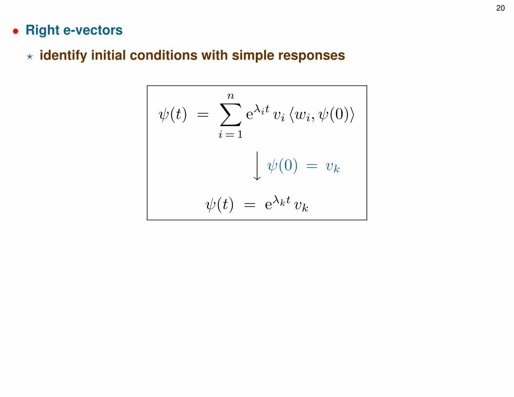
• Right e-vectors

? identify initial conditions with simple responses

ψ(t) =

n∑i= 1

eλit vi 〈wi, ψ(0)〉

y ψ(0) = vk

ψ(t) = eλkt vk

Dra

ft

M. JOVANOVIC 21

• E-value decomposition of A =

[ −1 0

k −2

]{v1 =

1√1 + k2

[1k

], v2 =

[01

]}{w1 =

[ √1 + k2

0

], w2 =

[−k1

]}

solution to ψ(t) = Aψ(t):

ψ(t) =(e−t v1w

∗1 + e−2t v2w

∗2

)ψ(0)

←−[

ψ1(t)

ψ2(t)

]=

[e−tψ1(0)

k(e−t − e−2t

)ψ1(0) + e−2tψ2(0)

]

• E-values: misleading measures of transient response

Dra

ft

M. JOVANOVIC 22

FORCED RESPONSES

Dra

ft

M. JOVANOVIC 23

Amplification of disturbances

• Harmonic forcing

d(t) = d(ω) eiωt steady-state response−−−−−−−−−−−−−−−−−−−→ φ(t) = φ(ω) eiωt

? Frequency response

φ(ω) = C (iωI − A)−1B︸ ︷︷ ︸

H(ω)

d(ω)

example: 3 inputs, 2 outputs

[φ1(ω)

φ2(ω)

]=

[H11(ω) H12(ω) H13(ω)H21(ω) H22(ω) H23(ω)

] d1(ω)

d2(ω)

d3(ω)

Hij(ω) – response from jth input to ith output

Dra

ft

M. JOVANOVIC 24

Input-output gains

• Determined by singular values of H(ω)

left and right singular vectors:

H(ω)H∗(ω)ui(ω) = σ2i (ω)ui(ω)

H∗(ω)H(ω) vi(ω) = σ2i (ω) vi(ω)

{ui} orthonormal basis of output space

{vi} orthonormal basis of input space

Dra

ft

M. JOVANOVIC 25

• Action of H(ω) on d(ω)

φ(ω) = H(ω) d(ω) =

r∑i= 1

σi(ω)ui(ω)⟨vi(ω), d(ω)

⟩

• Right singular vectors

? identify input directions with simple responses

σ1(ω) ≥ σ2(ω) ≥ · · · > 0

φ(ω) =

r∑i= 1

σi(ω)ui(ω)⟨vi(ω), d(ω)

⟩y d(ω) = vk(ω)

φ(ω) = σk(ω)uk(ω)

σ1(ω): the largest amplification at any frequency

Dra

ft

M. JOVANOVIC 26

Worst case amplification• H∞ norm: an induced L2 gain (of a system)

G = ‖H‖2∞ = maxoutput energyinput energy

= maxω

σ21 (H(ω))

σ2 1(H

(ω))

Dra

ft

M. JOVANOVIC 27

Robustness interpretation

-d Nominal

Linearized Dynamicss -

φ

�Γ

modeling uncertainty(can be nonlinear or time-varying)

• Closely related to pseudospectra of linear operators

ψ(t) = (A + B ΓC)ψ(t)

LARGEworst case amplification

⇒ small

stability margins

Dra

ft

M. JOVANOVIC 28

Back to a toy example[ψ1

ψ2

]=

[−λ1 0k −λ2

] [ψ1

ψ2

]+

[10

]d

G = maxω|H(iω)|2 =

k2

(λ1λ2)2

ROBUSTNESS

-d 1

s + λ1

-

ψ1

k -1

s + λ2

s -ψ2

�γ

modeling uncertainty

stability

mγ < λ1λ2/k

det

([s 00 s

]−[−λ1 γk −λ2

])= s2 + (λ1 + λ2) s + (λ1λ2 − γ k)︸ ︷︷ ︸

> 0

Dra

ft

M. JOVANOVIC 29

Response to stochastic forcing

• White-in-time forcing

E (d(t1) d∗(t2)) = I δ(t1 − t2)

? Hilbert-Schmidt norm

power spectral density:

‖H(ω)‖2HS = trace (H(ω)H∗(ω)) =

r∑i= 1

σ2i (ω)

? H2 norm

variance amplification:

‖H‖22 =1

2π

∫ ∞−∞‖H(ω)‖2HS dω =

∫ ∞0

‖H(t)‖2HS dt

Dra

ft

M. JOVANOVIC 30

Computation of H2 and H∞ norms

ψ(t) = Aψ(t) + B d(t)

φ(t) = C ψ(t)

• H2 norm

? Lyapunov equation

E (d(t1) d∗(t2)) = W δ(t1 − t2) ⇒{ ‖H‖22 = trace (C P C∗)

AP + P A∗ = −BWB∗

• H∞ norm

? E-value decomposition of Hamiltonian in conjunction with bisection

‖H‖∞ ≥ γ ⇔[

A 1γ BB

∗

−1γ C∗C −A∗

]has at least one imaginary e-value

Dra

ft

M. JOVANOVIC 31

BACK TO FLUIDS

Dra

ft

M. JOVANOVIC 32

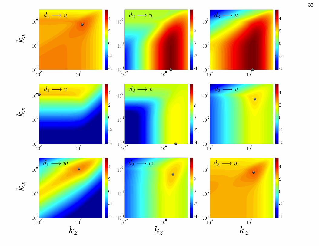
Frequency response: channel flow

harmonic forcing:

d(x, y, z, t) = d(kx, y, kz, ω) ei(kxx + kzz + ωt)ysteady-state response

v(x, y, z, t) = v(kx, y, kz, ω) ei(kxx + kzz + ωt)

• Frequency response: operator in y

-

d(kx, y, kz, ω)H(kx, kz, ω) -

v(kx, y, kz, ω)

? componentwise amplification uvw

=

Hu1 Hu2 Hu3

Hv1 Hv2 Hv3

Hw1 Hw2 Hw3

d1

d2

d3

Jovanovic & Bamieh, J. Fluid Mech. ’05

Dra

ft

M. JOVANOVIC 33

kx

kx

kx

kz kz kz

Dra

ft

M. JOVANOVIC 34

Amplification mechanism in flows with high Re

• HIGHEST AMPLIFICATION: (d2, d3)→ u

-

normal/spanwiseforcing

(sI − ∆−1∆2)−1

‘glorifieddiffusion’

- - ReAcp

vortextilting

- (sI − ∆)−1

viscousdissipation

-

streamwisevelocity

• LINEARIZED DYNAMICS OF NORMAL VORTICITY η

η = ∆η + ReAcp v

←−

source

Dra

ft

M. JOVANOVIC 35

+ AMPLIFICATION MECHANISM: vortex tilting or lift-up

wal

l-nor

mal

dire

ctio

n

spanwise direction

Dra

ft

M. JOVANOVIC 36

Linear analyses: Input-output vs. Stability

AMPLIFICATION:

v = H d

singular values of H

STABILITY:

ψ = Aψ

e-values of A

The cross sectional model

2 Dimensional, 3 Component (2D3C) model for parallel flowsDynamics of stream-wise constant pertrubations

• Simpler than full 3D models

• Has much of the phenomenology of boundary layer turbulence

– Transitional (bypass) and fully turbulent coherent structures arevery elongated in streamwise direction

typical structures cross sectional dynamics standard 2D models

8

typical structures cross-sectional dynamics 2D models

Dra

ft

M. JOVANOVIC 37

FLOW CONTROL

• Objective

? controlling the onset of turbulence

• Transition initiated by

? high flow sensitivity

• Control strategy

? reduce flow sensitivity

Dra

ft

M. JOVANOVIC 38

Sensor-free flow control

• GEOMETRY MODIFICATIONS

? riblets? surface roughness? super-hydrophobic surfaces

• BODY FORCES

? temporally/spatially oscillatory forces? traveling waves

• WALL OSCILLATIONS

? transverse wall oscillations

common theme: PDEs with spatially or temporally periodic coefficients

Dra

ft

M. JOVANOVIC 39

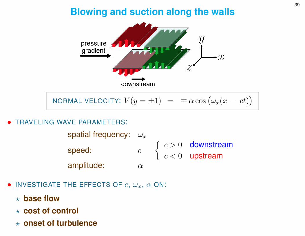
Blowing and suction along the walls

NORMAL VELOCITY: V (y = ±1) = ∓ α cos(ωx(x − ct)

)• TRAVELING WAVE PARAMETERS:

spatial frequency: ωx

speed: c

{c > 0 downstreamc < 0 upstream

amplitude: α

• INVESTIGATE THE EFFECTS OF c, ωx, α ON:

? base flow? cost of control? onset of turbulence

Dra

ft

M. JOVANOVIC 40

Min, Kang, Speyer, Kim, J. Fluid Mech. ’06

⇒ SUSTAINED SUB-LAMINAR DRAG

drag

timeCHALLENGE: selection of wave parameters

• THIS TALK:

? cost of control? onset of turbulence

Dra

ft

M. JOVANOVIC 41

Effects of blowing and suction?

• DESIRED EFFECTS OF CONTROL:

? bulk flux↗? net efficiency↗? fluctuations’ energy↘

TRAVELING WAVE

? induces a bulk flux (pumping)

PUMPING DIRECTION

? opposite to a traveling wave direction

Dra

ft

M. JOVANOVIC 42

Nominal velocity

V (y = ±1) = ∓α cos (ωx(x − ct))

= ∓α cos (ωx x)⇒

u = (U(x, y), V (x, y), 0)

steady in a traveling wave frameperiodic in x

• SMALL AMPLITUDE BLOWING/SUCTIONweakly-nonlinear analysis

U(x, y) =

parabola︷ ︸︸ ︷U0(y) + α2

mean drift︷ ︸︸ ︷U2,0(y) + α

oscillatory: no mean drift︷ ︸︸ ︷(U1,−1(y) e−iωxx + U1,1(y) eiωxx

)+ α2

(U2,−2(y) e−2iωxx + U2,2(y) e2iωxx

)+ O(α3)

Dra

ft

M. JOVANOVIC 43

Best-case scenario for net efficiency

ASSUME:

{no control: laminar

with control: laminar

ASSUME:

{no control: turbulent

with control: laminar

Dra

ft

M. JOVANOVIC 44

Velocity fluctuations: DNS preview

Lieu, Moarref, Jovanovic, J. Fluid Mech. ’10

Dra

ft

M. JOVANOVIC 45

Ensemble average energy density: controlled flow

EVOLUTION MODEL: linearization around (U(x, y), V (x, y), 0)

? periodic coefficients in x = x − ct

ψt = Aψ + B d

v = C ψ

} d = d(x, y, z, t) stochastic body forcingv = (u, v, w) velocity fluctuationsψ = (v, η) normal velocity/vorticity

Dra

ft

M. JOVANOVIC 46

• Simulation-free approach to determining energy density

Moarref & Jovanovic, J. Fluid Mech. ’10

effect of small wave amplitude:

energy density = energy density + α2︸︷︷︸small

E2(θ, kz;Re; ωx, c) + O(α4)

←−

←−

with control w/o control

(θ, kz) spatial wavenumbers

Dra

ft

M. JOVANOVIC 47

Energy amplification: controlled flow with Re = 2000

explicit formula:

energy density with controlenergy density w/o control

≈ 1 + α2 g2(θ, kz; ωx, c)

• (θ = 0, kz = 1.78): most energy w/o control

g2, downstream: g2, upstream:

Dra

ft

M. JOVANOVIC 48

Recap

facts revealed by perturbation analysis:

Blowing/Suction Type Nominal flow analysis Energy amplification analysis

Downstream reduce bulk flux reduce amplification XUpstream increase bulk flux X promote amplification

Moarref & Jovanovic, J. Fluid Mech. ’10

Dra

ft

M. JOVANOVIC 49

DNS results: avoidance/promotion of turbulence

small initial energy(flow with no control stays laminar)

DOWNSTREAM: NO TURBULENCE UPSTREAM: PROMOTES TURBULENCE

Dra

ft

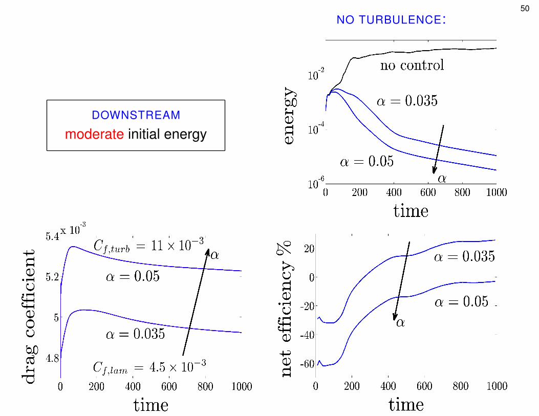
M. JOVANOVIC 50NO TURBULENCE:

DOWNSTREAM

moderate initial energy

Dra

ft

M. JOVANOVIC 51TURBULENCE:

UPSTREAM

moderate initial energy

Dra

ft

M. JOVANOVIC 52

OPTIMAL CONTROL AND ESTIMATION

Dra

ft

M. JOVANOVIC 53

Linear Quadratic Regulator (LQR)

• Minimize quadratic objective subject to linear dynamic constraint

minimize J(ψ, u) =1

2

∫ T

0

(〈ψ(τ), Qψ(τ)〉+ 〈u(τ), R u(τ)〉

)dτ +

1

2〈ψ(T ), QT ψ(T )〉

subject to Aψ(t) + B u(t) − ψ(t) = 0

ψ(0) = ψ0, t ∈ [0, T ]

? optimization variable is a function

u : [0, T ] −→ Hu

? state and control weights{Q, QT self-adjoint, non-negative

R self-adjoint, positive

? infinite number of constraints

Dra

ft

M. JOVANOVIC 54

• Introduce Lagrangian

L(ψ, u, λ) = J(ψ, u) +

∫ T

0

⟨λ(τ), Aψ(τ) + B u(τ) − ψ(τ)

⟩dτ

? form variations wrt ψ, u, λ

L(ψ, u+ u, λ) − L(ψ, u, λ) =

∫ T

0

〈Ru(τ) + B∗λ(τ), u(τ)〉dτ = 0

y has to hold for all u

u(t) = −R−1B∗λ(t), t ∈ [0, T ]

necessary conditions for optimality:

wrt λ ⇒ ψ(t) = Aψ(t) + B u(t), ψ(0) = ψ0

wrt ψ ⇒ λ(t) = −Qψ(t) − A∗ λ(t), λ(T ) = QT ψ(T )

wrt u ⇒ u(t) = −R−1B∗λ(t), t ∈ [0, T ]

Dra

ft

M. JOVANOVIC 55

Solution to finite horizon LQR

two-point boundary value problem:[ψ(t)

λ(t)

]=

[A −BR−1B∗

−Q −A∗] [

ψ(t)λ(t)

][ψ0

0

]=

[I 00 0

] [ψ(0)λ(0)

]+

[0 0QT −I

] [ψ(T )λ(T )

]u(t) = −R−1B∗λ(t)

• Differential Riccati Equation

can show: λ(t) = X(t)ψ(t)

−X(t) = A∗X(t) + X(t)A + Q − X(t)BR−1B∗X(t)

X(T ) = QT

? optimal controller: determined by state-feedback

u(t) = −K(t)ψ(t)

K(t) = R−1B∗X(t)

Dra

ft

M. JOVANOVIC 56

Infinite horizon LQR

minimize J =1

2

∫ ∞0

(〈ψ(τ), Qψ(τ)〉 + 〈u(τ), R u(τ)〉

)dτ

subject to ψ(t) = Aψ(t) + B u(t)

• Optimal controller:

{u(t) = −K ψ(t)

K = R−1B∗X

? X = X∗ – non-negative solution to Algebraic Riccati Equation (ARE)

A∗X + X A + Q − X BR−1B∗X = 0

(A,B) stabilizable(A,Q) detectable

}⇒ stability of ψ(t) = (A − BK)ψ(t)

Dra

ft

M. JOVANOVIC 57

Scalar example

ψ = aψ + u

J =1

2

∫ ∞0

(q ψ2(τ) + r u2(τ)

)dτ

• Optimal controller

klqr = a +

√a2 +

q

r⇒ ψ(t) = exp

(−√a2 +

q

rt

)ψ(0)

tradeoff:

large q/r small q/r

convergence rate fast X slowcontrol effort large low X

Dra

ft

M. JOVANOVIC 58

State-feedback H2 controller

minimize limt→∞

E(〈ψ(t), Qψ(t)〉 + 〈u(t), R u(t)〉

)subject to ψ(t) = Aψ(t) + Bd d(t) + Bu u(t)

E (d(t1) d∗(t2)) = Wd δ(t1 − t2)

• Minimum variance controller

state-feedback controller:

u(t) = −K ψ(t)

K = R−1B∗uX

0 = A∗X + X A + Q − X BuR−1B∗uX

Dra

ft

M. JOVANOVIC 59

State estimation

state equation: ψ(t) = Aψ(t) + Bd d(t) + Bu u(t)

measured output: ϕ(t) = C ψ(t) + n(t)

d(t) − process disturbance; n(t) − measurement noise

• Estimator (observer)

? copy of the system + linear injection term

˙ψ(t) = A ψ(t) + 0 · d(t) + Bu u(t) + L (ϕ(t) − ϕ(t))

ϕ(t) = C ψ(t) + 0 · n(t)

? estimation error: ψ(t) = ψ(t) − ψ(t)

˙ψ(t) = (A − LC) ψ(t) +

[Bd −L

] [ d(t)n(t)

]ϕ(t) = C ψ(t) + n(t)

(A,C) : detectable ⇒ can design L to provide stability of the error dynamics

Dra

ft

M. JOVANOVIC 60

Kalman filter

ψ(t) = Aψ(t) + Bd d(t) + Bu u(t)

ϕ(t) = C ψ(t) + n(t)

E (d(t1) d∗(t2)) = Wd δ(t1 − t2); E (n(t1)n∗(t2)) = Wn δ(t1 − t2)

• Kalman filter: optimal estimator

? minimizes steady-state variance of ψ(t) = ψ(t) − ψ(t)

Kalman gain:

L = Y C∗W−1n

0 = AY + Y A∗ + BdWdB∗d − Y C∗W−1

n C Y

Dra

ft

M. JOVANOVIC 61

Output-feedback H2 controller

minimize limt→∞

E(〈ψ(t), Qψ(t)〉 + 〈u(t), R u(t)〉

)subject to ψ(t) = Aψ(t) + Bd d(t) + Bu u(t)

ϕ(t) = C ψ(t) + n(t)

E (d(t1) d∗(t2)) = Wd δ(t1 − t2); E (n(t1)n∗(t2)) = Wn δ(t1 − t2)

• Minimum variance controller

observer-based controller:

˙ψ(t) = (A − LC) ψ(t) + Bu u(t) + Lϕ(t)

u(t) = −K ψ(t)

? feedback and observer gains:

{K LQR gain

L Kalman gain

Dra

ft

M. JOVANOVIC 62

H∞ controller

• BLENDS CLASSICAL WITH OPTIMAL CONTROL

-

finiteenergyinputs

Nominal Plant -

performanceoutputs

measuredoutputs

�Controller

controlinputs

-

�Modeling

Uncertainty

-

Dra

ft

M. JOVANOVIC 63

Boundary actuation• Example: heat equation

φt(y, t) = φyy(y, t) + d(y, t)

φ(−1, t) = u(t)

φ(+1, t) = 0

• Problem: control doesn’t enter additively into the equation

• Coordinate transformation

ψ(y, t) = φ(y, t) − f(y)u(t)

? Choose f(y) to obtain ψ(±1, t) = 0

? Many possible choices

Conditions for selection of f :

{f(−1) = 1, f(1) = 0} simple option−−−−−−−−−−−→ f(y) =1 − y

2

Dra

ft

M. JOVANOVIC 64

• In new coordinates:

φt(y, t) = φyy(y, t) + d(y, t)

φ(−1, t) = u(t)

φ(+1, t) = 0 yφ(y,t) = ψ(y,t) + f(y)u(t)

ψt(y, t) + f(y) u(t) = ψyy(y, t) + f ′′(y)u(t) + d(y, t)

ψ(±1, t) = 0

• New input: v(t) = u(t)

d

dt

[ψ(t)u(t)

]=

[A0 f ′′

0 0

] [ψ(t)u(t)

]+

[I0

]d(t) +

[−fI

]v(t)

φ(t) =[I f

] [ ψ(t)u(t)

]

A0 =d2

dy2with Dirichlet BCs

Dra

ft

M. JOVANOVIC 65

Blowing and suction along the walls

v(x,±1, z, t) =

∫ ∞−∞

∫ ∞−∞

∫ 1

−1

K±v (x− ξ, y, z − ζ) v(ξ, y, ζ, t) dy dξ dζ +

∫ ∞−∞

∫ ∞−∞

∫ 1

−1

K±η (x− ξ, y, z − ζ) η(ξ, y, ζ, t) dy dξ dζ

• Optimal controller: exponentially decaying convolution kernels

K−v (0− ξ, y, 0− ζ):

Hogberg, Bewley, Henningson, J. Fluid Mech. ’03

Dra

ft

M. JOVANOVIC 66

Optimal localized control• Blowing and suction along the discrete lattice

? DNS verification

Moarref, Lieu, Jovanovic, CTR Summer Program 2010

Dra

ft

M. JOVANOVIC 67

Sparsity-promoting optimal control

• Strike balance between quadratic performance and sparsity of K

minimize J(K) + γ card (K)

←−

←−

varianceamplification

sparsity-promotingpenalty function

• card (K) – number of non-zero elements of K

K =

5.1 −2.3 0 1.50 3.2 1.6 00 −4.3 1.8 5.2

⇒ card (K) = 8

• γ > 0 – quadratic performance vs. sparsity tradeoff

Lin, Fardad, Jovanovic, IEEE TAC ’11 (conditionally accepted; arXiv:1111.6188v1)

Dra

ft

M. JOVANOVIC 68

SUMMARY AND OUTLOOK

Dra

ft

M. JOVANOVIC 69

Summary: transition• INPUT-OUTPUT ANALYSIS

? quantifies flow sensitivity

? reveals distinct mechanisms for subcritical transitionstreamwise streaks, oblique waves, TS-waves

? exemplifies the importance of streamwise elongated flow structures

Jovanovic & Bamieh, J. Fluid Mech. ’05

• LATER STAGES OF TRANSITION

? challenge: relative roles of flow sensitivity and nonlinearitySelf-Sustaining Process (SSP)

O(1/R) O(1/R)

O(1)

Streaks

Streak wavemode (3D)

Streamwise

self−interactionnonlinear

U(y,z)instability of

Rolls

advection ofmean shear

WKH 1993, HKW 1995, W 1995, 1997

Waleffe, Phys. Fluids ’97 Farrell & Ioannou, CTR Summer Program ’12

Dra

ft

M. JOVANOVIC 70

Summary: sensor-free flow control

• CONTROLLING THE ONSET OF TURBULENCE

facts revealed by perturbation analysis:

Blowing/Suction Type Nominal flow analysis Energy amplification analysis

Downstream reduce bulk flux reduce amplification XUpstream increase bulk flux X promote amplification

• POWERFUL SIMULATION-FREE APPROACH TO PREDICTING FULL-SCALE RESULTS

? DNS verification

Moarref & Jovanovic, J. Fluid Mech. ’10

Lieu, Moarref, Jovanovic, J. Fluid Mech. ’10

Dra

ft

M. JOVANOVIC 71

Outlook: model-based sensor-free flow control

GEOMETRY MODIFICATIONS WALL OSCILLATIONS BODY FORCES

ribletssuper-hydrophobic surfaces

transverse oscillationsoscillatory forcestraveling waves

• USE DEVELOPED THEORY TO DESIGN GEOMETRIES AND WAVEFORMS FOR

? control of transition/skin-friction drag reduction

• CHALLENGES

? control-oriented modeling of turbulent flows

? optimal design of periodic waveforms

-Flow disturbances

Spatially Invariant PDE-

Fluctuations’ energy+

Cost of control

�Spatially Periodic

Multiplication

-

Dra

ft

M. JOVANOVIC 72

• CONTROL OF TURBULENT FLOWS

control-oriented modeling

model-based control design flow structures

Moarref & Jovanovic, J. Fluid Mech. ’12 (in press; arXiv:1206.0101)

Dra

ft

M. JOVANOVIC 73

Acknowledgments

TEAM:

Rashad Moarref Binh Lieu Armin Zare(Caltech) (U of M) (U of M)

SUPPORT:

NSF CAREER Award CMMI-06-44793NSF Award CMMI-09-27720U of M IREE Early Career AwardCTR Summer Programs ’06, ’10, ’12

COMPUTING RESOURCES:

Minnesota Supercomputing Institute

SPECIAL THANKS:

Prof. Moin