Embed Size (px)
Citation preview
Distributed Inference using Bounded Transmissions
by
Sivaraman Dasarathan
A Dissertation Presented in Partial Fulfillmentof the Requirements for the Degree
Doctor of Philosophy
Approved May 2013 by theGraduate Supervisory Committee:
Cihan Tepedelenlioglu, ChairAntonia Papandreou-Suppappola
Martin ReissleinMichael Goryll
ARIZONA STATE UNIVERSITY
August 2013
ABSTRACT
Distributed inference has applications in a wide range of fields such as
source localization, target detection, environment monitoring, and healthcare.
In this dissertation, distributed inference schemes which use bounded transmit
power are considered. The performance of the proposed schemes are studied
for a variety of inference problems.
In the first part of the dissertation, a distributed detection scheme
where the sensors transmit with constant modulus signals over a Gaussian
multiple access channel is considered. The deflection coefficient of the pro-
posed scheme is shown to depend on the characteristic function of the sensing
noise, and the error exponent for the system is derived using large devia-
tion theory. Optimization of the deflection coefficient and error exponent are
considered with respect to a transmission phase parameter for a variety of
sensing noise distributions including impulsive ones. The proposed scheme is
also favorably compared with existing amplify-and-forward (AF) and detect-
and-forward (DF) schemes. The effect of fading is shown to be detrimental
to the detection performance and simulations are provided to corroborate the
analytical results.
The second part of the dissertation studies a distributed inference
scheme which uses bounded transmission functions over a Gaussian multi-
ple access channel. The conditions on the transmission functions under which
consistent estimation and reliable detection are possible is characterized. For
the distributed estimation problem, an estimation scheme that uses bounded
transmission functions is proved to be strongly consistent provided that the
variance of the noise samples are bounded and that the transmission function
i
is one-to-one. The proposed estimation scheme is compared with the amplify
and forward technique and its robustness to impulsive sensing noise distribu-
tions is highlighted. It is also shown that bounded transmissions suffer from
inconsistent estimates if the sensing noise variance goes to infinity. For the
distributed detection problem, similar results are obtained by studying the
deflection coefficient. Simulations corroborate our analytical results.
In the third part of this dissertation, the problem of estimating the
average of samples distributed at the nodes of a sensor network is considered.
A distributed average consensus algorithm in which every sensor transmits
with bounded peak power is proposed. In the presence of communication
noise, it is shown that the nodes reach consensus asymptotically to a finite
random variable whose expectation is the desired sample average of the initial
observations with a variance that depends on the step size of the algorithm
and the variance of the communication noise. The asymptotic performance is
characterized by deriving the asymptotic covariance matrix using results from
stochastic approximation theory. It is shown that using bounded transmissions
results in slower convergence compared to the linear consensus algorithm based
on the Laplacian heuristic. Simulations corroborate our analytical findings.
Finally, a robust distributed average consensus algorithm in which ev-
ery sensor performs a nonlinear processing at the receiver is proposed. It is
shown that non-linearity at the receiver nodes makes the algorithm robust to
a wide range of channel noise distributions including the impulsive ones. It is
shown that the nodes reach consensus asymptotically and similar results are
obtained as in the case of transmit non-linearity. Simulations corroborate our
analytical findings and highlight the robustness of the proposed algorithm.
ii

ACKNOWLEDGEMENTS
First of all, I would like to express my sincere thanks and appreciation
to my advisor, Professor Cihan Tepedelenlioglu, whose valuable guidance and
support were essential for me to accomplish this work. In addition to aca-
demics, interaction with him has helped me develop several other skills which
will be useful throughout my life.
I would like to extend my thanks to all members of my committee, Pro-
fessors Antonia Papandreou-Suppappola, Martin Reisslein and Michael Goryll.
I would also take this opportunity to thank all the faculty members from whom
I have learned, including, but not limited to Professors Tolga Duman, Douglas
Cochran and Junshan Zhang. This work would not have been possible without
those course-works as the building blocks for my research.
I am also thankful to Professor Joseph Palais, and Clayton Javurek for
offering me financial assistantship throughout my graduate study. Thanks to
all the staff members of Electrical Engineering department; Darleen Mandt,
Esther Korner, Jenna Marturano, and Donna Rosenlof, to name just a few,
for their extraordinary kindness and infinite patience, they helped me every
time I visited them.
I express my thanks and appreciations to Mr.Mark Rentz, Jessica Jensen,
and Adin Armey of American English and Culture Program, ASU for provid-
ing me financial assistantship. Thanks to Senh Luu, Venkatesh Mandalapa,
and Sashi Gangaraju of University Technology Office, ASU for their constant
help and support I received from them at work.
I am grateful to all my friends and colleagues in the Signal Process-
ing and Communication group. Thanks to Adithya Rajan, Yuan Zhang,
iii

Junghoon Lee, Ruochen Zeng, Mahesh Banavar and Adarsh Narasimhamurthy
for their help and several useful discussions. Thanks to Professor Govin-
darajulu, Vijayavel Mohan, Jothi Sundaram, Ashok Kannaiyan, SenthilKu-
mar Kadirvelu, Sharada Ramesh, Ganesh Balasubramanian, Gokula Thu-
lasingam, Balaji Kadambi, Rajender Rajasekar, Hussain Mohammed, Irfan
Ahmed, Kabeer Ahmed, Sabil Ahmed, Malarvizhi Velappan and many other
friends who have supported and encouraged me during the most difficult times
of my graduate study.
Finally, my deepest gratitude goes to my parents, brother Muralidha-
ran Dasarathan and family members whose contributions cannot be mentioned
in words. I also offer my deepest gratitude to my Guru Bhagavan Sri Ramana
Maharishi whose Consciousness made a revolutionary change in the very na-
ture of my perception about life.
iv
TABLE OF CONTENTS
Page
LIST OF FIGURES . . . . . . . . . . . . . . . . . . . . . . . . . . . . ix
CHAPTER
1 Introduction . . . . . . . . . . . . . . . . . . . . . . . . . . . . . . . 1
1.1 Sensor Networks . . . . . . . . . . . . . . . . . . . . . . . . . . 1
1.1.1 Applications of Sensor Networks . . . . . . . . . . . . . 2
1.1.2 Architecture of Sensor Networks . . . . . . . . . . . . . 3
1.1.3 Design Challenges in WSNs . . . . . . . . . . . . . . . 8
1.2 Distributed Detection . . . . . . . . . . . . . . . . . . . . . . . 9
1.3 Distributed Estimation . . . . . . . . . . . . . . . . . . . . . . 14
1.4 Distributed Consensus . . . . . . . . . . . . . . . . . . . . . . 17
1.5 Contributions of the Dissertation . . . . . . . . . . . . . . . . 18
1.6 Outline of the Dissertation . . . . . . . . . . . . . . . . . . . . 21
2 Distributed Detection with Constant Modulus Signaling . . . . . . 22
2.1 Literature Survey and Motivation . . . . . . . . . . . . . . . . 22
2.2 System Model . . . . . . . . . . . . . . . . . . . . . . . . . . . 25
2.3 The Detection Problem . . . . . . . . . . . . . . . . . . . . . . 26
2.4 Probability of Error . . . . . . . . . . . . . . . . . . . . . . . . 27
2.5 Deflection Coefficient and its Optimization . . . . . . . . . . . 29
2.5.1 Optimizing D(ω) . . . . . . . . . . . . . . . . . . . . . 29
2.5.2 Finding the Optimum ω for Specific Noise Distributions 32
2.5.3 Per-sensor Power Constraint or high Channel SNR . . 36
2.5.4 Analysis of the DC for Non-homogeneous Sensors . . . 37
2.6 Fading Channels . . . . . . . . . . . . . . . . . . . . . . . . . 39
2.7 Asymptotic Performance and Optimization of ω based on error
exponent . . . . . . . . . . . . . . . . . . . . . . . . . . . . . . 41
2.8 Non-Gaussian Channel Noise . . . . . . . . . . . . . . . . . . . 43
v
CHAPTER Page
2.9 Simulations . . . . . . . . . . . . . . . . . . . . . . . . . . . . 44
2.9.1 Effect of ω on Performance . . . . . . . . . . . . . . . . 44
2.9.2 Comparison against MAF and MDF Schemes . . . . . 45
2.9.3 Total Power Constraint: Different Noise Distributions . 47
2.9.4 Error Exponent . . . . . . . . . . . . . . . . . . . . . . 48
2.9.5 Approximations of Pe(ω) through εω(z) . . . . . . . . . 51
2.9.6 Non-Gaussian Channel Noise . . . . . . . . . . . . . . 53
3 Distributed Inference with Bounded Transmissions . . . . . . . . . 56
3.1 Literature Survey and Motivation . . . . . . . . . . . . . . . . 56
3.2 Distributed Estimation with Bounded Transmissions . . . . . 59
3.2.1 System Model . . . . . . . . . . . . . . . . . . . . . . . 59
3.2.2 The Estimation Problem . . . . . . . . . . . . . . . . . 61
3.2.3 Asymptotic Normality of the Estimator . . . . . . . . . 66
3.2.4 Comparison with Amplify and Forward Scheme . . . . 67
3.3 Distributed Detection with Bounded Transmissions . . . . . . 69
3.3.1 System Model . . . . . . . . . . . . . . . . . . . . . . . 69
3.3.2 The Detection Problem . . . . . . . . . . . . . . . . . . 70
3.3.3 Probability of Error . . . . . . . . . . . . . . . . . . . . 70
3.3.4 Deflection Coefficient and its Optimization . . . . . . . 71
3.3.5 Locally Optimal Detection . . . . . . . . . . . . . . . . 76
3.4 Simulations . . . . . . . . . . . . . . . . . . . . . . . . . . . . 77
3.4.1 Distributed Estimation Performance . . . . . . . . . . 77
3.4.2 Distributed Detection Performance . . . . . . . . . . . 78
4 Distributed Consensus with Bounded Transmissions . . . . . . . . . 83
4.1 Literature Survey and Motivation . . . . . . . . . . . . . . . . 83
vi
CHAPTER Page
4.2 Review of Network Graph Theory . . . . . . . . . . . . . . . . 86
4.3 System Model and Previous Work . . . . . . . . . . . . . . . . 87
4.3.1 System Model . . . . . . . . . . . . . . . . . . . . . . . 87
4.3.2 Previous Work . . . . . . . . . . . . . . . . . . . . . . 87
4.4 Consensus with Bounded Transmissions and Communication
Noise . . . . . . . . . . . . . . . . . . . . . . . . . . . . . . . . 88
4.4.1 The NLC Algorithm with Communication Noise . . . . 89
4.4.2 A Result on the Convergence of Discrete time Markov
Processes . . . . . . . . . . . . . . . . . . . . . . . . . 91
4.4.3 Mean Square Error of NLC Algorithm . . . . . . . . . 98
4.4.4 Asymptotic Normality of NLC Algorithm . . . . . . . . 99
4.5 Simulations . . . . . . . . . . . . . . . . . . . . . . . . . . . . 103
4.5.1 Performance of NLC Algorithm without Channel Noise 104
4.5.2 Performance of NLC Algorithm with Channel Noise . . 105
4.6 Distributed Consensus on other Functions using NLC Algorithm 108
4.6.1 Distributed Variance and SNR Estimation . . . . . . . 109
4.6.2 Consensus on Arbitrary Functions . . . . . . . . . . . . 113
5 Robust Consensus with Receiver Non-Linearity . . . . . . . . . . . 115
5.1 Literature Survey and Motivation . . . . . . . . . . . . . . . . 115
5.2 System Model and Previous Work . . . . . . . . . . . . . . . . 117
5.2.1 System Model . . . . . . . . . . . . . . . . . . . . . . . 117
5.2.2 Previous Work . . . . . . . . . . . . . . . . . . . . . . 117
5.3 Robust Consensus with Impulsive Communication Noise . . . 118
5.3.1 The RNLC Algorithm with Communication Noise . . . 119
5.3.2 Mean Square Error of RNLC Algorithm . . . . . . . . 128
vii
CHAPTER Page
5.3.3 Asymptotic Normality of RNLC Algorithm . . . . . . . 129
5.4 Simulations . . . . . . . . . . . . . . . . . . . . . . . . . . . . 134
5.4.1 Performance of RNLC Algorithm Without Channel Noise135
5.4.2 Performance of RNLC Algorithm with Channel Noise . 136
6 Conclusions . . . . . . . . . . . . . . . . . . . . . . . . . . . . . . . 143
REFERENCES . . . . . . . . . . . . . . . . . . . . . . . . . . . . . . 147
viii
LIST OF FIGURES
Figure Page
1.1 Ad-hoc sensor network without fusion center. . . . . . . . . . . . 4
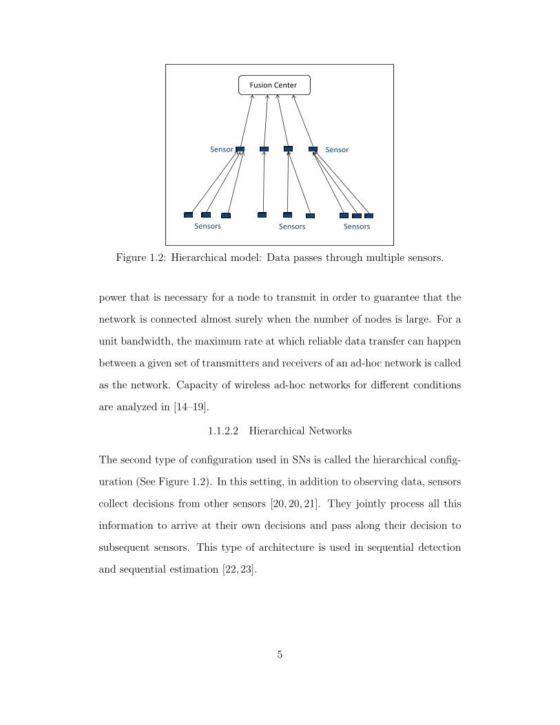
1.2 Hierarchical model: Data passes through multiple sensors. . . . . 5
1.3 Sensor network with a fusion center. . . . . . . . . . . . . . . . . 7
1.4 Distributed detection: Parallel topology with the fusion center . . 10
1.5 Parallel topology without the fusion center . . . . . . . . . . . . . 11
1.6 Serial topology . . . . . . . . . . . . . . . . . . . . . . . . . . . . 12
1.7 Tree topology . . . . . . . . . . . . . . . . . . . . . . . . . . . . . 13
1.8 Distributed detection: Multiple access topology with the fusion
center . . . . . . . . . . . . . . . . . . . . . . . . . . . . . . . . . 13
1.9 Distributed estimation: Parallel topology with the fusion center . 16
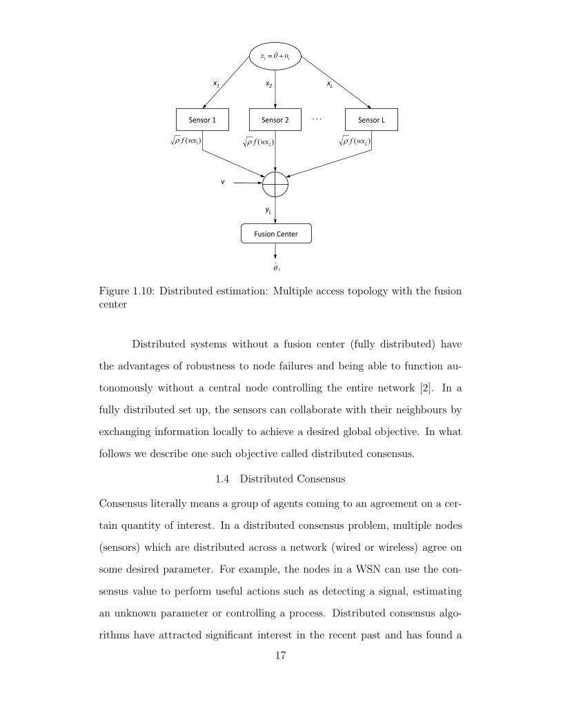
1.10 Distributed estimation: Multiple access topology with the fusion
center . . . . . . . . . . . . . . . . . . . . . . . . . . . . . . . . . 17
2.1 Total Power Constraint, D(ω), εω, Pe(ω) vs ω: ρs=10, 15 dB, ρc=-
10 dB, L=20 . . . . . . . . . . . . . . . . . . . . . . . . . . . . . 45
2.2 Per-sensor Power Constraint, Gaussian, Pe(ω) vs ω: ρs=-10 dB,
ρ=10 dB . . . . . . . . . . . . . . . . . . . . . . . . . . . . . . . . 46
2.3 Total Power Constraint, Pe vs ρs: ρ=-30 dB, L=60 . . . . . . . . 47
2.4 Total Power Constraint, Pe vs L: ρs=15 dB, ρc=0 dB . . . . . . . 48
2.5 Total Power Constraint, Pe vs L: ρs=5, 15 dB, ρc=-10 dB . . . . 49
2.6 Rayleigh flat fading, Pe vs ρc, ni Gaussian, L=10 . . . . . . . . . 50
2.7 Per-sensor Power Constraint, εω vs ρs . . . . . . . . . . . . . . . . 51
2.8 Total Power Constraint, εω vs ρc: ρs=0, 10 dB, σ2v=1 . . . . . . . 52
2.9 Gaussian Sensing Noise: Pe vs ρc: ρs=0 dB, L=10, 20, 40, 60 . . . 53
2.10 Gaussian Sensing Noise: Pe vs ρc: ρs=10 dB, L=5, 7 . . . . . . . 54
ix
Figure Page
2.11 Mixed Gaussian channel noise: εω vs ρc: σ2v0=0.25, p0 = 0.8, σ2
v1=4,
p1 = 0.2, σ2veff
= 1, ρs=0 dB. . . . . . . . . . . . . . . . . . . . . . 54
2.12 Gaussian Sensing Noise: Pe vs ρs: PT=-12.22 dB, L=60 . . . . . . 55
3.1 Bounded transmissions over Gaussian multiple access channel . . 61
3.2 Total Power Constraint: f(x) = tanh(ωx), σ2n=1, σ2
v=1, PT=10,
L=500 . . . . . . . . . . . . . . . . . . . . . . . . . . . . . . . . . 78
3.3 Total Power Constraint, ni Laplacian: f(x) = tanh(ωx), σ2n=1,
σ2v=1, PT=10, L=25, 50, 500 . . . . . . . . . . . . . . . . . . . . . 79
3.4 Total Power Constraint: f(x) = tanh(ωx), σ2n=1, σ2
v=1, ρ=1, ω=0.75 80
3.5 Total Power Constraint, Different bounded functions: σ2n=1, σ2
v=1,
PT=10, L=500 . . . . . . . . . . . . . . . . . . . . . . . . . . . . 81
3.6 Total Power Constraint, f(x) = tanh(ωx), D(ω) Pe(ω) versus ω,
ρs = 10 dB, ρc = 3 dB, L=20 . . . . . . . . . . . . . . . . . . . . 81
3.7 Total Power Constraint, ni Gaussian, Pe versus L, ρs = 10 dB,
ρc = 0 dB . . . . . . . . . . . . . . . . . . . . . . . . . . . . . . . 82
4.1 Entries of X(t) versus Iterations t: α = 1.5, ω = 0.01, N = 75,
h(x) = tanh(ωx), x = 76. . . . . . . . . . . . . . . . . . . . . . . . 104
4.2 Evolution of error ||X(t) − x1|| versus Iterations t: α = 1.5, ω =
0.01, N = 75, x = 76. . . . . . . . . . . . . . . . . . . . . . . . . . 105
4.3 Evolution of error ||X(t) − x1|| versus Iterations t: α = 2, 4, 6, 8,
ω = 0.005, N = 75, h(x) = 2πtan−1[sinh(π
2ωx)], x = 114. . . . . . 106
4.4 Entries of X(t) versus Iterations t: h(x) =√ρ tanh(ωx), ω = 0.05,
N = 10, x = 36.24, ρ = 10 dB, σ2v = 1. . . . . . . . . . . . . . . . 107
4.5 Transmit power h2(xi(t)) per-neighbour versus Iterations t: h(x) =
√ρ tanh(ωx), ω = 0.005, N = 75, x = 102, ρ = 7.5 dB, σ2
v = 0.1. . 108
x
Figure Page
4.6 ||E[X(t)]− x1|| versus Iterations t: h1(x) =√ρ tan−1(ωx), h2(x) =
√ρ tanh(ωx), ω = 0.005, N = 75, x = 162, 202, ρ = 7.5 dB, σ2
v = 1. 109
4.7 ||E[X(t)] − x1|| versus Iterations t: ω = 0.04, N = 10, x = 36.24,
ρ = 5 dB, σ2v = 1. . . . . . . . . . . . . . . . . . . . . . . . . . . . 110
4.8 ||E[X(t)] − x1|| versus ρ: h(x) =√ρ ωx√
1+ω2x2, ω = 0.006, N = 75,
x = 77, Iterations t = 20, 40, 60, 80, σ2v = 1. . . . . . . . . . . . . . 111
4.9 Total power versus Variance of xi(0): ni is Gaussian, θ = 2, N =
75, h(x) = x, σ2 = 0.01. . . . . . . . . . . . . . . . . . . . . . . . 113
4.10 Total power versus Variance of xi(0): ni is Laplacian, θ = 2, N =
75, h(x) = x, σ2 = 0.01. . . . . . . . . . . . . . . . . . . . . . . . 114
5.1 Entries of X(t) versus Iterations t: α = 100, N = 15, h(x) =
tanh(0.05x), f(x) = 2πtan−1(π
20.05x), x = 22.67. . . . . . . . . . . 134
5.2 Evolution of error ||X(t) − x1|| versus Iterations t: α = 100, ω =
0.05, N = 15, x = 22.67. . . . . . . . . . . . . . . . . . . . . . . . 135
5.3 Entries of X(t) versus Iterations t: Cauchy noise, h(x) = x, f(x) =
x, N = 75, x = 134.31, γ = 1. . . . . . . . . . . . . . . . . . . . . 136
5.4 Entries of X(t) versus t: Cauchy noise, h(x) =√ρ 2πtan−1(π
20.01x),
f(x) = tanh(5x), N = 10, x = 43.96, ρ = 15 dB, γ = 0.1. . . . . . 137
5.5 Entries of X(t) versus t: Cauchy noise, h(x) =√ρ 2πtan−1(π
20.01x),
f(x) = tanh(5x), N = 75, x = 134.31, ρ = 5 dB, γ = 0.1. . . . . . 138
5.6 ||E[X(t)] − x1|| versus Iterations t: f(x) = 1.5x1+|1.5x| , ω = 0.01,
N = 75, x = 134.31, ρ = 10 dB, γ = 0.413. . . . . . . . . . . . . . 139
5.7 ||E[X(t)]− x1|| versus Iterations t: Cauchy noise, h(x) = x, f(x) =
1.5x1+|1.5x| , N = 75, x = 84.31, γ = 0.413. . . . . . . . . . . . . . . . . 140
xi
Figure Page
5.8 ||E[X(t)] − x1|| versus Iterations t: h(x) = x, ω = 1.5, N = 10,
x = 34.31, γ = 0.413. . . . . . . . . . . . . . . . . . . . . . . . . . 141
5.9 ||E[X(t)] − x1|| versus Iterations t: Robustness to various noise
distributions, h(x) = x, f(x) = tanh(2x), N = 75, x = 124.31 . . 142
5.10 Entries of X(t) versus Iterations t: Difference between Variance
of θ∗ and Asymptotic Variance, h(x) = x, f(x) = 3 tan−1(0.05x),
N = 75, x = 94.31, γ = 0.413 . . . . . . . . . . . . . . . . . . . . 142
xii
Chapter 1
Introduction
1.1 Sensor Networks
Sensor networks (SNs) are designed to observe and collect information about a
phenomenon of interest by using sensor nodes deployed in space. The configu-
ration of the network depends on the application requirements such as health,
military and home applications [1–3]. The nodes in a sensor network typi-
cally have sensing, processing and communication capabilities, that can help
make intelligent decisions. Depending on the nature of the application and the
types of sensors, a sensor network can be designed to observe a single physical
phenomenon, or a single network can be designed to collect information from
various physical conditions. Recent advancements in electronics and hardware
technology have enabled the development of small, low cost, low power sen-
sors. These devices have the capability of wireless communications and some
of them are capable of locomotion. These features make the sensor networks
suitable for a variety of applications discussed in Section 1.1.1.
The size of sensor nodes can range from being extremely small (of
the order of cubic-millimetre) called as the smart-dust [4] to large platforms
collecting telemetry information in a aircraft. Depending on how the sensor
nodes are used and deployed, their capabilities may vary widely. Extremely
small sensors have limited memory capacity [1], they may be able to do sensing
but may not have sophisticated signal processing capabilities. Larger sensor
nodes that are supported by a more complex infrastructure can have more
sophisticated and different types of sensors. These can also be supported by
larger computers with better computing capacities [5].
1
Wireless sensor networks (WSNs) differ fundamentally from general
data networks such as the internet, and there are challenging problems in
designing such networks. Some of the issues briefly follow. The local sensor
observations need to be processed (compressed) before they are sent to the
fusion center for joint processing. This arises for example, if the range of the
observed data at local sensors is large, or the channel capacity between sensors
and the fusion center is limited. If, on the other hand, the raw data observed
at local sensors are accessible in their entirety at the fusion center, the problem
of studying the physical phenomenon could be solved by one of the techniques
of classical statistical inference [6, 7]. The system should operate with the
stringent power constraints imposed by the WSN. The communication among
the sensors and between the sensors and the fusion center should happen
through the unreliable wireless channels.
1.1.1 Applications of Sensor Networks
Numerous applications of SNs have been discussed in detail in [2]. Due to the
advances in the past decade in microelectronics, sensing, analog and digital
signal processing, wireless communications, and networking, the design chal-
lenges are being tackled and WSNs are expected to have significant impact on
lives of people in the twenty-first century. WSNs can be an integral part of
military command, control, communications, computing, intelligence, surveil-
lance, reconnaissance and targeting systems. There are many environmental
applications such as forest fire detection, bio-complexity mapping of the envi-
ronment, flood detection and precision agriculture etc. WSNs have significant
number of health applications such as tele-monitoring of human physiological
data, tracking and monitoring doctors and patients inside a hospital drug ad-
ministration in hospitals. These applications involve identification of certain
2
signal sources that may be characteristics of hazardous material, monitoring
chemicals near a volcano, temperatures in a furnace, shifts in undersea tec-
tonic plates, or explosives in the air, to mention a few. Thus, SNs provide
a safe and low-cost inference alternative. Interesting commercial applications
include environmental control in office buildings, interactive museums, detect-
ing and monitoring car thefts, managing inventory control and vehicle tracking
and detection. Sensor networks can also be used for traffic control [8]. They
can be used to inform drivers about the areas of congestion, and to divert
the traffic to increase the efficiency of the roadways. They can be used to
monitor roads for accidents and stoppages. SNs can be deployed to manage
parking areas and to detect illegal use of parking areas. There are applications
in manufacturing, transportation, and home appliances in which multiple de-
cision makers arise naturally. Therefore, the study and design of distributed
methods for distributed inference in WSNs becomes an important subject.
1.1.2 Architecture of Sensor Networks
There are three different architectures for sensor networks; 1). Ad-hoc Net-
works, 2). Hierarchical Networks and 3). Conventional Sensor Networks.
These are briefly discussed here.
1.1.2.1 Ad-hoc Networks
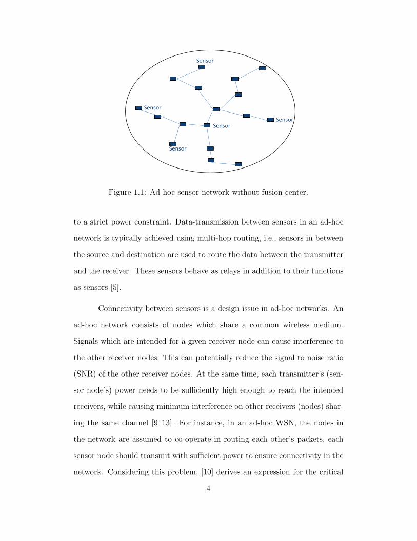
In network literature, ad-hoc networks (Figure 1.1) refer to devices placed to
form a network without a controlling base station. These devices discover each
other and cooperate intelligently in order to function as a network. The ad-
hoc sensor networks are constructed in the same manner. Low-power sensors
are placed in an observation field and the sensor network exists without a
fusion center. Algorithms are developed for diverse applications such as data
routing, collaborative inference and distributed signal processing, all subject
3
Sensor
Sensor
Sensor
Sensor
Sensor
Figure 1.1: Ad-hoc sensor network without fusion center.
to a strict power constraint. Data-transmission between sensors in an ad-hoc
network is typically achieved using multi-hop routing, i.e., sensors in between
the source and destination are used to route the data between the transmitter
and the receiver. These sensors behave as relays in addition to their functions
as sensors [5].
Connectivity between sensors is a design issue in ad-hoc networks. An
ad-hoc network consists of nodes which share a common wireless medium.
Signals which are intended for a given receiver node can cause interference to
the other receiver nodes. This can potentially reduce the signal to noise ratio
(SNR) of the other receiver nodes. At the same time, each transmitter’s (sen-
sor node’s) power needs to be sufficiently high enough to reach the intended
receivers, while causing minimum interference on other receivers (nodes) shar-
ing the same channel [9–13]. For instance, in an ad-hoc WSN, the nodes in
the network are assumed to co-operate in routing each other’s packets, each
sensor node should transmit with sufficient power to ensure connectivity in the
network. Considering this problem, [10] derives an expression for the critical
4
Fusion Center
Sensor
Sensors Sensors Sensors
Sensor
Figure 1.2: Hierarchical model: Data passes through multiple sensors.
power that is necessary for a node to transmit in order to guarantee that the
network is connected almost surely when the number of nodes is large. For a
unit bandwidth, the maximum rate at which reliable data transfer can happen
between a given set of transmitters and receivers of an ad-hoc network is called
as the network. Capacity of wireless ad-hoc networks for different conditions
are analyzed in [14–19].
1.1.2.2 Hierarchical Networks
The second type of configuration used in SNs is called the hierarchical config-
uration (See Figure 1.2). In this setting, in addition to observing data, sensors
collect decisions from other sensors [20, 20, 21]. They jointly process all this
information to arrive at their own decisions and pass along their decision to
subsequent sensors. This type of architecture is used in sequential detection
and sequential estimation [22, 23].
5
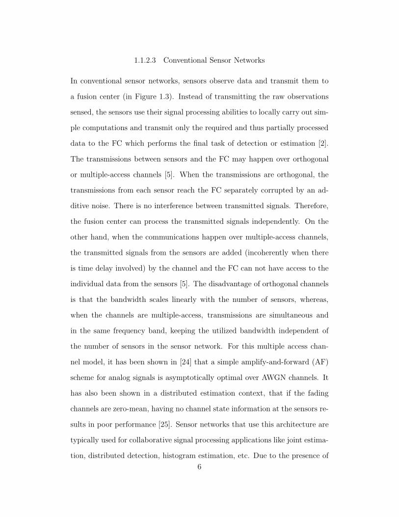
1.1.2.3 Conventional Sensor Networks
In conventional sensor networks, sensors observe data and transmit them to
a fusion center (in Figure 1.3). Instead of transmitting the raw observations
sensed, the sensors use their signal processing abilities to locally carry out sim-
ple computations and transmit only the required and thus partially processed
data to the FC which performs the final task of detection or estimation [2].
The transmissions between sensors and the FC may happen over orthogonal
or multiple-access channels [5]. When the transmissions are orthogonal, the
transmissions from each sensor reach the FC separately corrupted by an ad-
ditive noise. There is no interference between transmitted signals. Therefore,
the fusion center can process the transmitted signals independently. On the
other hand, when the communications happen over multiple-access channels,
the transmitted signals from the sensors are added (incoherently when there
is time delay involved) by the channel and the FC can not have access to the
individual data from the sensors [5]. The disadvantage of orthogonal channels
is that the bandwidth scales linearly with the number of sensors, whereas,
when the channels are multiple-access, transmissions are simultaneous and
in the same frequency band, keeping the utilized bandwidth independent of
the number of sensors in the sensor network. For this multiple access chan-
nel model, it has been shown in [24] that a simple amplify-and-forward (AF)
scheme for analog signals is asymptotically optimal over AWGN channels. It
has also been shown in a distributed estimation context, that if the fading
channels are zero-mean, having no channel state information at the sensors re-
sults in poor performance [25]. Sensor networks that use this architecture are
typically used for collaborative signal processing applications like joint estima-
tion, distributed detection, histogram estimation, etc. Due to the presence of
6
Sensor
Fusion Center
Sensor Sensor
Sensor
Sensor
Sensor
Sensor
Figure 1.3: Sensor network with a fusion center.
multiple sensors, statistical methods perform very well since the number of ob-
servations can be very large. Histogram estimation using type based multiple
access (TBMA) is introduced in [26].
Transmissions from the sensors to the FC can be analog or digital [5].
The digital method consists of quantizing the sensed data and then trans-
mitting the data digitally over a rate-constrained channel [27]. In this case,
the required channel bandwidth is quantified by the number of bits being
transmitted between the sensors and the fusion center. When the number of
quantization levels is high to reduce the loss of information, the bandwidth
requirements increases for transmitting the information digitally. If the band-
width is limited, analog methods of transmissions may be used. One such
analog method consists of amplifying and then forwarding the sensed data to
the FC, while imposing a power constraint [25]. The transmissions can be
appropriately pulse-shaped and amplitude modulated to consume finite band-
width. The major drawback of the amplify-and-forward scheme is that the
transmit power depends on the sensing noise realizations and therefore may
7
not be bounded. One solution to this problem is the use of phase modulation
techniques with constant modulus transmissions from the sensors. Another
solution is to map the sensed observations through a bounded function before
transmission so that the transmit power is always constrained.
1.1.3 Design Challenges in WSNs
The three major design principles for energy-constrained WSNs are summa-
rized below (please see [1, 28–32] for detailed discussions).
1. Low Power Constraints: Exploit low power hardware, and external
assets, to the greatest extent possible.
2. Communication Constraints: Optimize distributed detection and
estimation network tasks while minimizing the use of communications.
3. Network Constraints: Support network specific goals while minimizing
idle listening, network set-up, and network maintenance.
One of the most important constraints that is faced when dealing with
autonomous nodes is that these nodes are severely power limited [1,2]. In most
cases, the nodes are supplied with power with batteries when deployed and
these batteries cannot be recharged or replaced. Typically energy consumption
depends on the state of the sensor node, such as transmit, receive, idle etc. For
instance, it is shown in [33] that the transceiver of the sensor node consumes
more power in receive mode than in transmit mode. Since these nodes may
be deployed in remote regions, it is preferred that they stay powered for large
periods of time before the nodes are replaced. Therefore, whenever nodes are
autonomously deployed, the algorithms used on the nodes have to be designed
to consume minimal power so that the battery life can be maximized. It should
be noted here that while computing operations do consume power, maximum
power is consumed by the transceivers on the nodes. Hence, there is a need
8
for efficient multi-access schemes to maximize transfer of information subject
to strict power constraints. When the sensors are deployed individually, they
can perform only simple computations and perform poorly at sensing. How-
ever, when deployed in large numbers, they can collaborate among themselves
to form intelligent networks and complicated tasks using statistical inference
could be accomplished. A number of useful references for various other design
issues such time synchronization, node localization, medium access control,
hardware and routing in an energy constrained WSN, are enumerated in [1].
In this work, we consider several distributed inference problems with
bounded transmit power from the sensors. Statistical inference can be broadly
classified into hypothesis testing and estimation. Accordingly, there are two
areas of distributed signal processing: Distributed detection and Distributed
estimation. In what follows, a brief overview of these two areas with some of
the relevant literature is described.
1.2 Distributed Detection
In a classical centralized detection scheme, the local sensors are assumed to
communicate their observations to a central processor that performs the task
of optimal detection using conventional statistical techniques. This is an ideal
scenario without loss of information and noise free communication is assumed
between the sensors and the central processor. In a distributed detection sys-
tem, generally, the raw observations are processed (quantized and channel
coded in case of digital transmissions) at the local sensors before they are
transmitted to the fusion center. This results in loss of information (often
referred to as lossy compression) at the local sensors and further loss could
occur if the transmission is over a fading/noisy channel. For these reasons,
the performance of a distributed detection system will always be suboptimal
9
H0/H1
. . .
Fusion Center
Sensor L
nL
Sensor 2
n2
Sensor 1
n1
yL yL y2
uL u1 u2
u0
Figure 1.4: Distributed detection: Parallel topology with the fusion center
compared to the centralized detection system. However, there are significant
advantages of the distributed detection such as reduced bandwidth require-
ment (due to lossy compression), increased reliability, and reduced cost. In
addition, due to the relatively low cost of sensors, the availability of high speed
communication networks, and increased computational capability, distributed
detection has become a topic of great research interest [34] in the last two
decades. There are four different topologies used for distributed detection: 1).
Parallel topology, 2). Serial topology, 3). Tree topology, and 4). Multiple
access topology [22, 35–38].
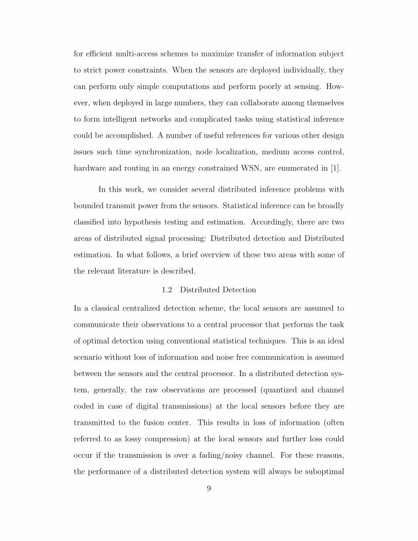
Figure 1.4 shows a simple parallel topology with a fusion center. In this
study, we are concerned with the binary hypothesis testing problem for the
detection problem. There are basically L sensors in this system. Each sensor
observes the phenomenon and independently takes its decision based on its
local decision rule. Here, x1, . . . , xL are the observations of the L sensors
and u1, . . . , uL are their corresponding decisions. Each sensor then transmits
10
S1
x1
S2
x2
SL-1
xL-1
SL
xL
Phenomenon H
. . . . . . .
u1
u2
uL-1
uL
Figure 1.5: Parallel topology without the fusion center
its decision to the fusion center over a dedicated orthogonal channel and n1,
. . . , nL are the additive noise samples associated with the reception of u1, . . . ,
uL respectively. Here it is clear that L parallel channels are needed. So, as
the number of sensors increase, the bandwidth requirements for the successful
operation of the network would increase greatly. The fusion center’s task is
to decide which one of the hypothesis is true by jointly processing the noisy
versions of the decisions u1, . . . , uL received across the L branches. In a
more general setting, u1, . . . , uL could be functions of x1, . . . , xL respectively
instead of the binary decisions of the individual sensors. Note that there is
information loss in this general setting as well, and therefore the performance
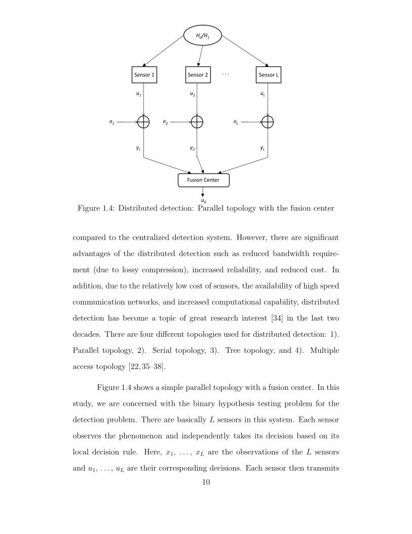
at the FC will be sub-optimal compared to the centralized set-up. Figure 1.5
shows a DD system without a fusion center. All the sensors observe a common
phenomenon and make local decisions about the phenomenon. There is no task
of fusion in this setting, whereas costs of decision making at different sensors
are assumed to be coupled and a system wide optimization is performed based
on the coupled cost function [22].
11
S1
x1
S2
x2
SL-1
xL-1
SL
xL
Phenomenon H
. . . .
. . . . . . .
u1
u2
uL-2
uL-1
u0
Figure 1.6: Serial topology
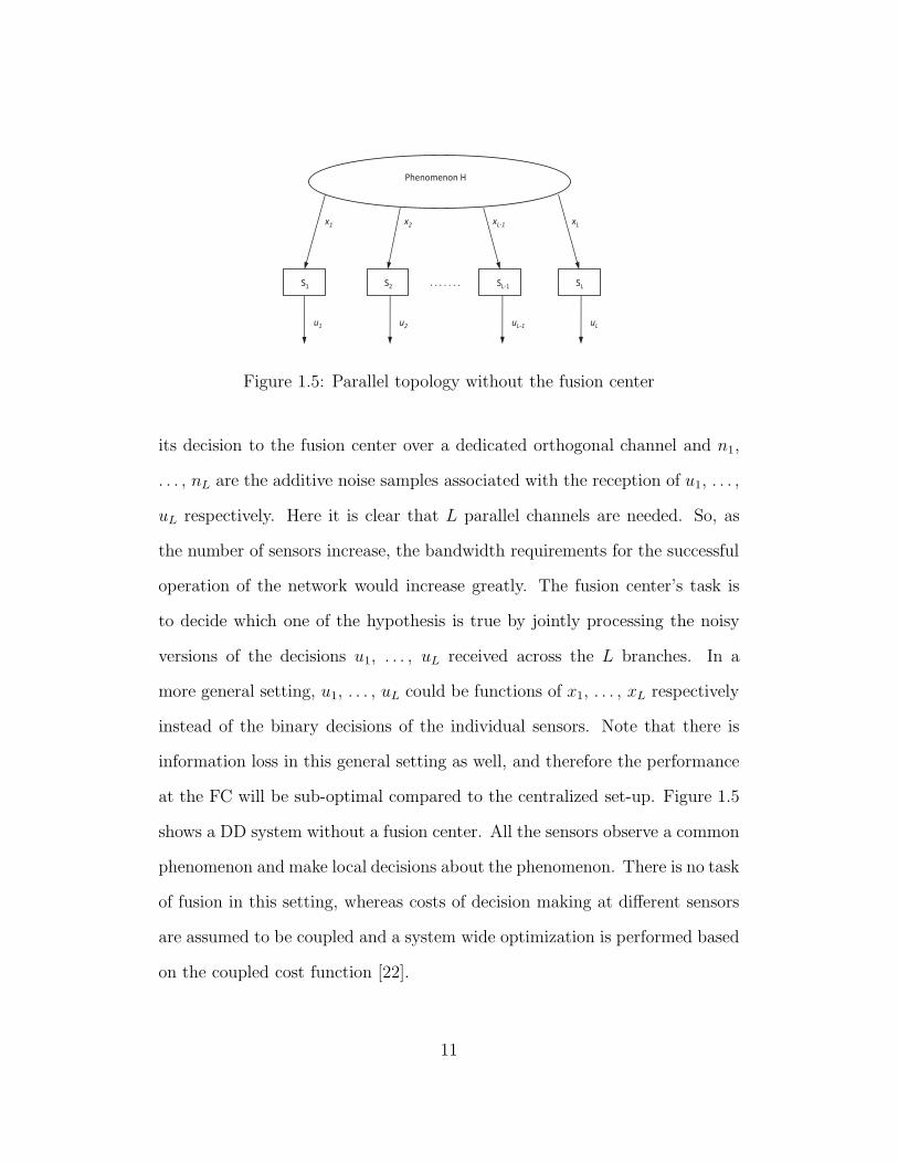
Figure 1.6 shows the Serial Topology for a distributed detection system.
In this setting, the decisions of the individual sensors are combined in a serial
manner. For instance, consider the case of only two sensors. First sensor
1 observes x1 and takes a decision u1. This decision is given to sensor 2
which takes the final decision by combining its own observation x2 and the
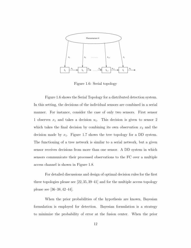
decision made by x1. Figure 1.7 shows the tree topology for a DD system.
The functioning of a tree network is similar to a serial network, but a given
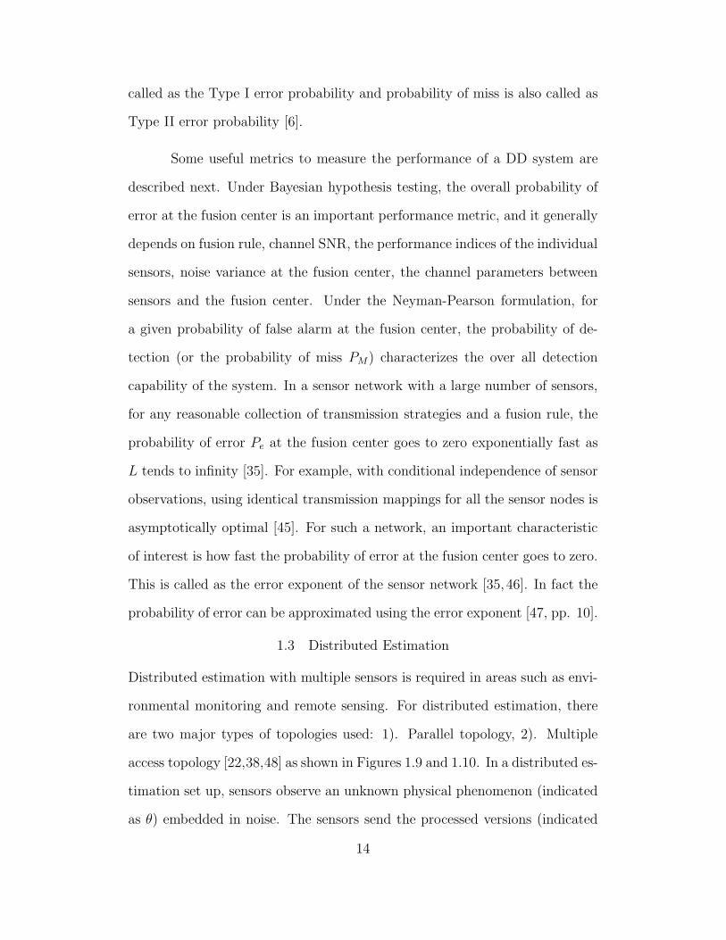
sensor receives decisions from more than one sensor. A DD system in which
sensors communicate their processed observations to the FC over a multiple
access channel is shown in Figure 1.8.
For detailed discussions and design of optimal decision rules for the first
three topologies please see [22,35,39–41] and for the multiple access topology
please see [36–38, 42–44].
When the prior probabilities of the hypothesis are known, Bayesian
formulation is employed for detection. Bayesian formulation is a strategy
to minimize the probability of error at the fusion center. When the prior
12
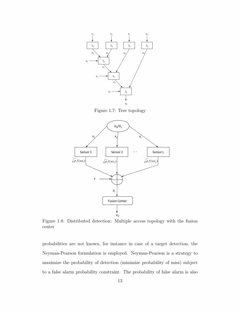
S3
S4
S5
S6
S2
S1
S0
u0
u3
u6
u5
u4
u2
u1
x3
x4
x5
x6
x2
x0
x1
Figure 1.7: Tree topology
H0/H1
Fusion Center
v
. . . Sensor L Sensor 2 Sensor 1
u0
x1 x2
xL
yL
)( 2wxfr )( Lwxfr)( 1wxfr
Figure 1.8: Distributed detection: Multiple access topology with the fusioncenter
probabilities are not known, for instance in case of a target detection, the
Neyman-Pearson formulation is employed. Neyman-Pearson is a strategy to
maximize the probability of detection (minimize probability of miss) subject
to a false alarm probability constraint. The probability of false alarm is also
13
called as the Type I error probability and probability of miss is also called as
Type II error probability [6].
Some useful metrics to measure the performance of a DD system are
described next. Under Bayesian hypothesis testing, the overall probability of
error at the fusion center is an important performance metric, and it generally
depends on fusion rule, channel SNR, the performance indices of the individual
sensors, noise variance at the fusion center, the channel parameters between
sensors and the fusion center. Under the Neyman-Pearson formulation, for
a given probability of false alarm at the fusion center, the probability of de-
tection (or the probability of miss PM) characterizes the over all detection
capability of the system. In a sensor network with a large number of sensors,
for any reasonable collection of transmission strategies and a fusion rule, the
probability of error Pe at the fusion center goes to zero exponentially fast as
L tends to infinity [35]. For example, with conditional independence of sensor
observations, using identical transmission mappings for all the sensor nodes is
asymptotically optimal [45]. For such a network, an important characteristic
of interest is how fast the probability of error at the fusion center goes to zero.
This is called as the error exponent of the sensor network [35, 46]. In fact the
probability of error can be approximated using the error exponent [47, pp. 10].
1.3 Distributed Estimation
Distributed estimation with multiple sensors is required in areas such as envi-
ronmental monitoring and remote sensing. For distributed estimation, there
are two major types of topologies used: 1). Parallel topology, 2). Multiple
access topology [22,38,48] as shown in Figures 1.9 and 1.10. In a distributed es-
timation set up, sensors observe an unknown physical phenomenon (indicated
as θ) embedded in noise. The sensors send the processed versions (indicated
14
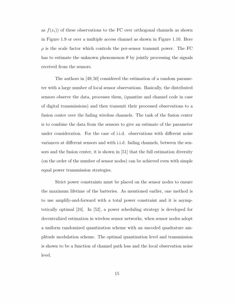
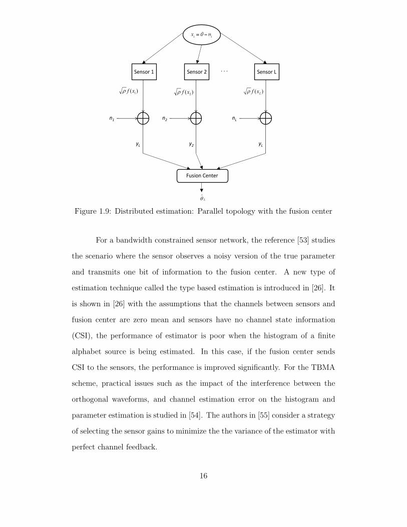
as f(xi)) of these observations to the FC over orthogonal channels as shown
in Figure 1.9 or over a multiple access channel as shown in Figure 1.10. Here
ρ is the scale factor which controls the per-sensor transmit power. The FC
has to estimate the unknown phenomenon θ by jointly processing the signals
received from the sensors.
The authors in [49,50] considered the estimation of a random parame-
ter with a large number of local sensor observations. Basically, the distributed
sensors observe the data, processes them, (quantize and channel code in case
of digital transmissions) and then transmit their processed observations to a
fusion center over the fading wireless channels. The task of the fusion center
is to combine the data from the sensors to give an estimate of the parameter
under consideration. For the case of i.i.d. observations with different noise
variances at different sensors and with i.i.d. fading channels, between the sen-
sors and the fusion center, it is shown in [51] that the full estimation diversity
(on the order of the number of sensor nodes) can be achieved even with simple
equal power transmission strategies.
Strict power constraints must be placed on the sensor nodes to ensure
the maximum lifetime of the batteries. As mentioned earlier, one method is
to use amplify-and-forward with a total power constraint and it is asymp-
totically optimal [24]. In [52], a power scheduling strategy is developed for
decentralized estimation in wireless sensor networks, when sensor nodes adopt
a uniform randomized quantization scheme with an uncoded quadrature am-
plitude modulation scheme. The optimal quantization level and transmission
is shown to be a function of channel path loss and the local observation noise
level.
15
. . .
Fusion Center
Sensor L
nL
Sensor 2
n2
Sensor 1
n1
yL yL y2
)( 1xfr )( 2xfr )( Lxfr
L
Ù
q
Figure 1.9: Distributed estimation: Parallel topology with the fusion center
For a bandwidth constrained sensor network, the reference [53] studies
the scenario where the sensor observes a noisy version of the true parameter
and transmits one bit of information to the fusion center. A new type of
estimation technique called the type based estimation is introduced in [26]. It
is shown in [26] with the assumptions that the channels between sensors and
fusion center are zero mean and sensors have no channel state information
(CSI), the performance of estimator is poor when the histogram of a finite
alphabet source is being estimated. In this case, if the fusion center sends
CSI to the sensors, the performance is improved significantly. For the TBMA
scheme, practical issues such as the impact of the interference between the
orthogonal waveforms, and channel estimation error on the histogram and
parameter estimation is studied in [54]. The authors in [55] consider a strategy
of selecting the sensor gains to minimize the the variance of the estimator with
perfect channel feedback.
16
Fusion Center
v
. . . Sensor L Sensor 2 Sensor 1
x1 x2
xL
yL
)( 2wxfr )( Lwxfr)( 1wxfr
L
Ù
q
Figure 1.10: Distributed estimation: Multiple access topology with the fusioncenter
Distributed systems without a fusion center (fully distributed) have
the advantages of robustness to node failures and being able to function au-
tonomously without a central node controlling the entire network [2]. In a
fully distributed set up, the sensors can collaborate with their neighbours by
exchanging information locally to achieve a desired global objective. In what
follows we describe one such objective called distributed consensus.
1.4 Distributed Consensus
Consensus literally means a group of agents coming to an agreement on a cer-
tain quantity of interest. In a distributed consensus problem, multiple nodes
(sensors) which are distributed across a network (wired or wireless) agree on
some desired parameter. For example, the nodes in a WSN can use the con-
sensus value to perform useful actions such as detecting a signal, estimating
an unknown parameter or controlling a process. Distributed consensus algo-
rithms have attracted significant interest in the recent past and has found a
17
wide range of applications [56–58]. Here we introduce the basic idea behind
distributed consensus algorithm in a WSN.
Consider a WSN with N sensors deployed with sensing, communication
and signal processing capabilities. Let each sensor hold an initial measurement
xi(0) ∈ R, i = 1, . . . , N , measured by each of the N sensors. The measure-
ments could contain information about the unknown parameters of a physical
phenomenon such as temperature or strength of an unknown signal. Let the
average of the initial measurements x = N−1∑N
i=1 xi(0) be the parameter to
be estimated by a distributed algorithm, in which each node communicates
only with its neighbours. If the states of all the sensor nodes converge asymp-
totically with time to x, then the network is said to have reached consensus
on the sample average.
Distributed average consensus algorithms have been considered in the
literature (please see [58–67] and references therein). In most of these papers,
it is assumed that a given node can obtain exact information of the state
values of its neighbours through local communications. This essentially means
that there is unlimited energy and/or bandwidth. However, as mentioned in
Section 1.1.3, practical WSNs are severely power limited and the available
bandwidth is finite. Therefore, there is a need for consensus algorithms which
could work under strict resource constraints of power and bandwidth imposed
by the WSNs.
1.5 Contributions of the Dissertation
In this work, we address the first two design challenges discussed in Section
1.1.3 by proposing distributed detection and estimation schemes which require
bounded transmit power and finite bandwidth. The proposed schemes will
18
be shown to outperform the existing schemes under the stringent power and
bandwidth constraints imposed by WSNs.
A distributed detection scheme relying on constant modulus transmis-
sions from the sensors is proposed over a Gaussian multiple access channel.
The instantaneous transmit power does not depend on the random sensing
noise, which is a desirable feature for low-power sensors with limited peak
power capabilities. In addition to the desirable constant-power feature, the
proposed detector is robust to impulsive noise, and performs well even when
the moments of the sensing noise do not exist as in the case of the Cauchy
distribution. It is shown that over Gaussian multiple access channels, the pro-
posed detector outperforms AF, DF and modified DF schemes consistently,
and the modified AF scheme when the sensing SNR is greater than 4 dB. The
proposed detector is shown to perform well even when the channel noise is
non-Gaussian. The error exponent is also derived for the proposed scheme
and large deviation theory is used to approximate the probability of error for
large L.
A distributed inference scheme which uses bounded transmission func-
tions over a Gaussian multiple access channel is considered. The conditions
on the transmission functions under which consistent estimation and reliable
detection are possible is characterized. For the distributed estimation prob-
lem, an estimation scheme that uses bounded transmission functions is proved
to be strongly consistent provided that the variance of the noise samples are
bounded and that the transmission function is one-to-one. The asymptotic
variance is derived, and shown to depend on the derivative of the transmission
function and the sensing noise statistics and channel noise variance. The pro-
posed estimation scheme is compared with the amplify and forward technique
19
and its robustness to impulsive sensing noise distributions is highlighted. It
is also shown that bounded transmissions suffer from inconsistent estimates
if the sensing noise variance goes to infinity. For the distributed detection
problem, similar results are obtained by studying the deflection coefficient.
A distributed average consensus algorithm in which every sensor trans-
mits with bounded peak power is proposed. In the presence of communication
noise, it is shown that the nodes reach consensus asymptotically to a finite
random variable whose expectation is the desired sample average of the initial
observations with a variance that depends on the step size of the algorithm
and the variance of the communication noise. The asymptotic performance is
characterized by deriving the asymptotic covariance matrix using results from
stochastic approximation theory. It is shown that using bounded transmissions
results in slower convergence compared to the linear consensus algorithm based
on the Laplacian heuristic.
A distributed average consensus algorithm in which every sensor per-
forms a nonlinear processing at the receiver is proposed. We prove that non-
linearity at the receiver nodes makes the algorithm robust to a wide range of
channel noise distributions including the impulsive ones. This work is the first
of its kind in the literature to propose a consensus algorithm which relaxes the
requirement of finite moments on the communication noise. When the com-
munication noise samples are i.i.d., it is shown that the nodes reach consensus
asymptotically to a finite random variable whose expectation is the desired
sample average of the initial observations with a variance that depends on the
step size of the algorithm and the receiver nonlinear function. The asymptotic
performance is characterized by deriving the asymptotic covariance matrix
using results from stochastic approximation theory. It is shown that scaling
20
the receiver nonlinear function does not affect the convergence speed of the
algorithm. An interesting relationship between the Fisher information and the
asymptotic covariance matrix is shown.
1.6 Outline of the Dissertation
The rest of the Dissertation is organized as follows. Chapter 2 describes a dis-
tributed detection scheme relying on constant modulus transmissions from the
sensors over a Gaussian multiple access channel and analyses the performance
of the proposed detection scheme by deriving the deflection coefficient and
the error exponent for several cases. Chapter 3 considers a general problem
of distributed inference using bounded transmission functions and establish
regimes under which estimation and detection will be possible and discuss
regimes under which estimation will fail and reliable detection will be impos-
sible. Chapter 4 studies the merits and demerits of bounded transmissions in
distributed consensus problems and characterizes the performance for a variety
of bounded transmission functions. Chapter 5 proposes a robust consensus al-
gorithm and characterizes its asymptotic performance. Finally the conclusions
are presented in Chapter 6.
21
Chapter 2
Distributed Detection with Constant Modulus Signaling
2.1 Literature Survey and Motivation
In Chapter 1 we learnt that, in inference-based wireless sensor networks, low-
power sensors with limited battery and peak power capabilities transmit their
observations to a fusion center (FC) for detection of events or estimation of
parameters. For distributed detection, much of the literature has focused on
the parallel topology where each sensor uses a dedicated channel to transmit
to a fusion center. Multiple access channels offer bandwidth efficiency since
the sensors transmit over the same time/frequency slot.
In [68], the distributed detection over a multiple access channel is stud-
ied where arbitrary number of quantization levels at the local sensors are
allowed, and transmission from the sensors to the fusion center is subject
to both noise and inter-channel interference. References [69–72] discuss dis-
tributed detection over Gaussian multiple access channels. In [69], detection
of a deterministic signal in correlated Gaussian noise and detection of a first-
order autoregressive signal in independent Gaussian noise are studied using an
amplify-and-forward scheme where the performance of different fusion rules is
analyzed. In [70], a type-based multiple access scheme is considered in which
the local mapping rule encodes a waveform according to the type [73, pp. 347]
of the sensor observation and its performance under both the per-sensor and
total power constraints is investigated. This scheme is extended to the case
of fading between the sensors and the FC in [71] and its performance is an-
alyzed using large deviation theory. In the presence of non-coherent fading
over a Gaussian multi-access channel, type-based random access is proposed
and analyzed in [72]. In [74], the optimal distributed detection scheme in a
22
clustered multi-hop sensor network is considered where a large number of dis-
tributed sensor nodes quantize their observations to make local hard decisions
about an event. The optimal decision rule at the cluster head is shown to be a
threshold test on the weighted sum of the local decisions and its performance
is analysed.
Two schemes called modified amplify-and-forward (MAF) and the mod-
ified detect-and-forward (MDF) are developed in [37] which generalize and
outperform the classic amplify-and-forward (AF) and detect-and-forward (DF)
approaches to distributed detection. It is shown that MAF outperforms MDF
when the number of sensors is large and the opposite conclusion is true when
the number of sensors is smaller. For the MDF scheme with identical sensors,
the optimal decision rule is proved to be a threshold test in [36]. Decision
fusion with a non-coherent fading Gaussian multiple access channel is con-
sidered in [75] where the optimal fusion rule is shown to be a threshold test
on the received signal power and on-off keying is proved to be the optimal
modulation scheme. A distributed detection system where sensors transmit
their observations over a fading Gaussian multiple-access channel to a FC
with multiple antennas using amplify-and-forward is studied in [76]. In all
these cases, the sensing noise distribution is assumed to be Gaussian. Even
though the Gaussian assumption is widely used, sensor networks which oper-
ate in adverse conditions require detectors which are robust to non-Gaussian
scenarios. Moreover, in the literature there has been little emphasis on dis-
tributed schemes with the desirable feature of using constant modulus signals
with fixed instantaneous power.
A distributed estimation scheme where the sensor transmissions have
constant modulus signals is considered in [38]. Distributed estimation in a
23
bandwidth-constrained sensor network with a noisy channel is investigated
in [77] and distributed estimation of a vector signal in a sensor network with
power and bandwidth constraints is studied in [78]. The estimator proposed
in [38] is shown to be strongly consistent for any sensing noise distribution
in the iid case. Inspired by the robustness of this estimation scheme, in this
work, a distributed detection scheme where the sensors transmit with constant
modulus signals over a Gaussian multiple access channel is proposed for a bi-
nary hypothesis testing problem. The sensors transmit with constant modulus
transmissions whose phase is linear with the sensed data. The output-signal-
to-noise-ratio, also called as the deflection coefficient (DC) of the system, is
derived and expressed in terms of the characteristic function (CF) of the sens-
ing noise. The optimization of the DC with respect to the transmit phase
parameter is considered for different distributions on the sensing noise includ-
ing impulsive ones. The error exponent is also derived and shown to depend
on the CF of the sensing noise. It is shown that both the DC and the error
exponent can be used as accurate predictors of the phase parameter that min-
imizes the detection error rate. The proposed detector is favorably compared
with MAF and the MDF schemes developed in [36,37] for the Gaussian sensing
noise and its robustness in the presence of other sensing noise distributions is
highlighted. The effect of fading between the sensors and the fusion center
is shown to be detrimental to the detection performance through a reduction
in the DC depending on the fading statistics. Different than [38] where the
asymptotic variance of an estimator is analyzed, the emphasis herein is on
derivation, analysis, and optimization of detection-theoretic metrics such as
the DC and error exponent. Our aim in this chapter is to develop a distributed
detection scheme where the instantaneous transmit power is not influenced by
possibly unbounded sensor measurement noise.24
This chapter is organized as follows. In Section 2.2, the system model
is described with per-sensor power constraint and total power constraint. In
Section 2.3, the detection problem is described and a linear detector is pro-
posed. The probability of error performance of the detector is analyzed in
Section 2.4. The DC is defined and its optimization for several cases is stud-
ied in Section 2.5. The presence of fading between the sensors and the fusion
center is discussed in Section 2.6. The error exponent of the proposed detec-
tor is analyzed in Section 2.7. Non-Gaussian channel noises are discussed in
Section 2.8. Simulation results are provided in Section 2.9 which support the
theoretical results.
2.2 System Model
Consider a binary hypothesis testing problem with two hypotheses H0, H1
where P0, P1 are their respective prior probabilities. Let the sensed signal at
the ith sensor be,
xi =
θ + ni underH1
ni underH0
(2.1)
i = 1, . . . , L, θ > 0 1 is a known parameter whose presence or absence has
to be detected, L is the total number of sensors in the system, and ni is the
noise sample at the ith sensor. The sensing noise samples are independent,
have zero median and an absolutely continuous distribution but they need not
be identically distributed or have any finite moments. We consider a setting
where the ith sensor transmits its measurement using a constant modulus signal
√ρejωxi over a Gaussian multiple access channel so that the received signal at
1the proposed scheme will work without any difference for θ < 0 due to symmetry if wesubstitute −θ in the place of θ in all the equations.
25
the FC is given by
yL =√ρ
L∑
i=1
ejωxi + v (2.2)
where ρ is the power at each sensor, ω > 0 is a design parameter to be
optimized and v ∼ CN (0, σ2v) is the additive channel noise. We consider
two types of power constraints: Per-sensor power constraint and total power
constraint. In the former case, each sensor has a fixed power ρ so that the
total power PT = ρL, and as L → ∞, PT → ∞; in the later case, the total
power PT is fixed for the entire system and does not depend on L, so that the
per-sensor power ρ = PT/L → 0 as L → ∞.
2.3 The Detection Problem
The received signal yL under the total power constraint can be written as
yL =
√PT
L
L∑
i=1
ejωxi + v. (2.3)
We assume throughout that P0 = P1 = 0.5 for convenience even though other
choices can be easily incorporated. With the received signal in (2.3), the FC
has to decide which hypothesis is true. It is well known that the optimal fusion
rule under the Bayesian formulation is given by:
f(yL|H1)
f(yL|H0)
H1
≷H0
P0
P1= 1 (2.4)
where f(yL|Hi), is the conditional probability density function of yL when Hi
is true. The equation (2.3) can be rewritten as follows:
yL =
√PT
L
(L∑
i=1
cos(ωxi)
)+ j
√PT
L
(L∑
i=1
sin(ωxi)
)+ v.
Since there are L terms in the first summation involving the cosine function,
we need to do L fold convolutions with the PDFs of cos(ωxi) and another set of
L fold convolutions with the PDFs of sin(ωxi). Then we need to find the joint
26
distribution of the PDFs obtained thus for the cosine and sine counterparts.
This joint PDF will need to be convolved with the PDF of v. It is not possible
to obtain a closed form expression for these (2L+1) fold convolutions. Hence,
f(yL|Hi) is not tractable. Therefore, we consider the following linear detector
which is argued next to be optimal for large L:
ℜ[yLe−jωθ]− ℜ[yL]H1
≷H0
0 , (2.5)
where we define ℜ[y] as the real part, and ℑ[y] as the imaginary part of
y. Note that the detector in (2.5) would be optimal if yL were Gaussian.
Clearly due to central limit theorem yL in (2.3) is asymptotically Gaussian,
which indicates that (2.5) approximates (2.4) for large L. With the Gaussian
assumption, the variances of yL in (2.3) under the two hypotheses are the same
and given by Var(yL|H0) =Var(yL|H1) = [PT(1−ϕ2n(ω))+σ2
v ], where ϕn(ω) is
the characteristic function of ni. Hence, the optimal likelihood ratio simplifies
to the detector in (2.5) which is linear in yL, when yL is assumed Gaussian
which holds for large L. However as will be seen in Section 2.4, we do not
assume that yL is Gaussian for any fixed L when we analyze the performance
of the detector in (2.5) or in finding the associated error exponent in Section
2.7. We proceed by expressing the probability of error.
2.4 Probability of Error
The detector in (2.5) depends on the design parameter ω and this means that
the probability of error will in turn depend on ω. Let Pe(ω) be the probability
of error at the FC:
Pe(ω) =1
2Pr [error|H0] +
1
2Pr [error|H1] = Pr [error|H0] (2.6)
where Pr [error|Hi] is the error probability when Hi, i ∈ {0, 1}, is true and
the last equality holds due to symmetry between the two hypotheses which is27
explained as follows. From the detection rule (2.5), the probability of error
under H0 is given by
Pr [error|H0] = Pr[ℜ[yL] < ℜ[yLe−jωθ]|H0
], (2.7)
where the received signal in (2.3) under H0 is given by
yL =
√PT
L
L∑
i=1
ejωni + v. (2.8)
Substituting (2.8) for yL in (2.7) and doing some algebraic simplifications,
Pr [error|H0] can be written as
Pr
L∑
i=1
2 sin
(ωθ
2
)cos
(ωni −
ωθ
2+
π
2
)+
√L
PTvT
︸ ︷︷ ︸ZL(ω):=
< 0
(2.9)
where vT := ℜ[v](1− cos(ωθ))−ℑ[v] sin(ωθ). Similarly, Pr [error|H1] is same
as that of (2.9) except the argument of the cosine function is replaced by
(ωni + ωθ/2 − π/2). To see the symmetry between the two hypotheses as-
serted in (2.6), let ζ := (ωθ/2− π/2) for convenience, so that cos(ωni ∓ ζ) =
[cos(ωni) cos ζ + sin(±ωni) sin ζ ]. Since ni is symmetric, ωni and −ωni have
the same distribution which implies that the random variables cos(ωni − ζ)
and cos(ωni + ζ) have the same distribution establishing that Pr [error|H1] =
Pr [error|H0]. Therefore, the probability of error in (2.6) is given by (2.9). We
are interested in using (2.9) to find the ω that minimizes the probability of
error at FC. Since Pe(ω) is not straightforward to evaluate, we optimize two
surrogate metrics to select ω. These are the error exponent and the DC. The
error exponent is an asymptotic measure of how fast the Pe(ω) decreases as
L → ∞, and is specific to the detector used in (2.5) and will be considered in
28

Section 2.7. The DC, on the other hand, is specific to the model in (2.3), and
does not depend on any detector.
2.5 Deflection Coefficient and its Optimization
We will now define and use the deflection coefficient which reflects the output-
signal-to-noise-ratio and widely used in optimizing detectors [79–82]. The DC
is mathematically defined as,
D(ω) :=1
L
|E[yL|H1]− E[yL|H0]|2var[yL|H0]
. (2.10)
By calculating the expectations in (2.10), it can be easily verified that the DC
for the signal model in (2.2) is given by:
D(ω) =2ϕ2
n(ω)[1− cos(ωθ)][1− ϕ2
n(ω) +σ2v
PT
] (2.11)
where ϕn(ω) = E[ejωni] is the CF of ni. The CF ϕn(ω) does not depend
on the sensor index i, since we will be initially assuming that ni are iid.
We will consider the non-identically distributed case in Section 2.5.4. Note
that D(ω) ≥ 0 and that ϕn(ω) is real-valued since ni is a symmetric random
variable. Moreover, ϕn(ω) = ϕn(−ω) so that D(ω) = D(−ω) which justifies
why we will focus on ω > 0 throughout. The factor (1/L) introduced in (2.10)
does not appear in conventional definitions of the DC but included here for
simplicity since it does not affect the optimal ω.
2.5.1 Optimizing D(ω)
We are now interested in finding ω by optimizing D(ω):
ω∗ := argmaxω>0
D(ω). (2.12)
Since ϕn(ω) ≤ 1, when σ2v > 0, D(ω) is bounded, and achieves its small-
est value of D(ω) = 0 as ω → 0. On the other hand, as ω → ∞, we29
have limω→∞D(ω) = 0. This implies that the maximum in (2.12) cannot
be achieved by ω = 0 or ω = ∞ and establishes that there must be a finite
ω∗ ∈ (0,∞) which attains the maximum in (2.12).
In what follows, we will further characterize ω∗ by assuming that ϕn(ω)
¿ 0 and ϕ′
n(ω) < 0 for all ω > 0. Many distributions including the Laplace,
Gaussian and Cauchy have CFs that satisfy this assumption. Indeed all sym-
metric alpha-stable distributions [83, pp. 20] of which the latter two is a
special case, satisfy this assumption. We now have the following theorem
which restricts ω∗ in (2.12) to a finite interval.
Theorem 2.5.1. If ϕn(ω) is decreasing and differentiable over ω > 0, then
ω∗ ∈ (0, π/θ).
Proof. First, note that ϕn(ω) ≥ 0 which is implied by the assumption that
ϕn(ω) is decreasing and that ϕn(ω) → 0 as ω → ∞. Let D(ω) = C(ω)[1 −
cos(ωθ)] with C(ω) := 2ϕ2n(ω)/[1 − ϕ2
n(ω) + σ2v/PT] for brevity. Since ϕn(ω)
is decreasing on ω > 0 and ϕn(ω) ≥ 0, C(ω) is also decreasing. Because
[1− cos(ωθ)] is periodic in ω with period 2π/θ,
D
(ω +
2π
θ
)= [1− cos(ωθ)]C
(ω +
2π
θ
)< [1− cos(ωθ)]C(ω) = D(ω).
(2.13)
Noticing that D(2π/θ) = 0 which rules out ω∗ = 2π/θ, we have ω∗ ∈ (0, 2π/θ).
To further reduce the range of ω∗ by half, consider the fact that D(0) =
D(2π/θ) = 0, which combined with D(ω) > 0 for ω ∈ (0, 2π/θ) implies that
ω∗ ∈ (0, 2π/θ) satisfies D′
(ω∗) = 0. Writing D′
(ω∗) = 0 we obtain:
[θ sin(ω∗θ)]
[cos(ω∗θ)− 1]=
C′
(ω∗)
C(ω∗). (2.14)
Since C(ω) > 0 is decreasing, the right hand side (rhs) of (2.14) is negative
and it follows that ω∗ ∈ (0, π/θ) as required.30
By the definition of ω∗, it is clearly a function of θ. We showed in
Theorem 2.5.1 that 0 < ω∗ < π/θ if ϕ′
n(ω) < 0 for ω > 0. Note that when
ω = 0, there is no phase modulation done, and what is transmitted is a
constant signal which actually contains no information about xi. Therefore
the boundary value ω = 0 is not a valid choice. When ω = π/θ, the detector
in (2.5) actually simplifies to: ℜ[yL]H0
≷H1
0. While ω = π/θ is a valid choice,
it is optimal only when θ is large as will be proved in Theorem 2. We now
investigate the behavior of ω∗ when θ is large without assuming anything
about ϕn(ω) except the absolute continuity of its distribution, and show that
ω∗ ≈ π/θ for large θ in the sense that ω∗θ → π, as θ → ∞.
Theorem 2.5.2. If σ2v > 0, and ni are iid and have absolutely continuous
distributions,
limθ→∞
ω∗θ = π. (2.15)
Proof. We have
D(πθ
)≤ D(ω∗) ≤ sup
ω>0[1− cos(ωθ)] sup
ω>0C(ω) =
4PT
σ2v
, (2.16)
where the first inequality is because ω∗ maximizes D(ω), and the second in-
equality follows fromD(ω) = C(ω)[1−cos(ωθ)]. Recalling that limω→0 ϕn(ω) =
1 we take the limit as θ → ∞ in (2.11) and obtain limθ→∞D(π/θ) = 4PT/σ2v ,
which using (2.16) shows that limθ→∞D(ω∗) = 4PT/σ2v . Since ϕn(0) > ϕn(ω)
and because D(ω) is an increasing function of ϕ2n(ω), from (2.11) it is clear
that the only way limθ→∞D(ω∗) = 4PT/σ2v holds is if ω∗ → 0 and ω∗θ → π,
as θ → ∞.
Theorem 2.5.2 establishes that when θ is large we have an approximate
closed-form solution for ω∗ ≈ π/θ for any absolutely continuous sensing noise
distribution.31
2.5.2 Finding the Optimum ω for Specific Noise Distributions
Theorem 2.5.1 showed that ω∗ ∈ (0, π/θ) for a general class of distributions.
Under more general conditions, Theorem 2.5.2 establishes that ω∗ ≈ π/θ when
θ is large. To find ω∗ exactly, we need to specify the sensing noise distribu-
tion through its CF, ϕn(ω). In what follows we describe how to find ω∗ for
several specific but widely used sensing noise distributions. We will assume
throughout that the assumptions of Theorem 2.5.1 (ϕ′
n(ω) < 0 for ω > 0) are
satisfied so that ω∗ ∈ (0, π/θ), which holds for Gaussian, Cauchy and Lapla-
cian distributions, among others. We will assume σ2v > 0 throughout this
subsection.
2.5.2.1 Gaussian Sensing Noise
In this case, we have ϕn(ω) = e−ω2σ2n/2 so that ϕ2
n(ω) = e−ω2σ2n, where σ2
n is the
variance of ni. To simplify (2.11) we substitute β = ωθ. Since ω ∈ (0, π/θ)
we have β ∈ (0, π). Note that the value of ω that maximizes (2.11) over ω
is related to the β that maximizes D(β/θ) through the relation ω = β/θ.
Differentiating D(β/θ) with respect to β, equating to 0 and simplifying we
obtain,
GG(β) := α− e−σ2n
θ2β2 − 2ασ2
n
θ2β tan
(β
2
)= 0 (2.17)
with α := [1 + (σ2v/PT)]. Equation (2.17) can not be solved in closed-form.
However it does have a unique solution in β ∈ (0, π) as shown below.
First we note that GG(0) = (α−1) > 0 since σ2v > 0 and GG(π) = −∞.
Since GG(β) is continuous, (2.17) has at least one solution. To show that this
solution is unique, consider the first derivative:
G′
G(β) =σ2n
θ2
[2βe−
σ2n
θ2β2 − 2α
(β
2sec2
(β
2
)+ tan
(β
2
))]. (2.18)
32
Now, using tan(β/2) ≥ β/2 and sec2(β/2) ≥ 1 + (β2/4) for β ∈ (0, π), we get
the following upper bound:
G′
G(β) ≤σ2n
θ2
[2βe−
σ2n
θ2β2 − αβ
(1 +
β2
4
)− αβ
]. (2.19)
Since σ2v > 0 we have α > 1. Recall that β ∈ (0, π), and the rhs of (2.19)
is always negative. It follows that GG(β) is monotonically decreasing over
β ∈ (0, π) and (2.17) has a unique solution which corresponds to the global
maximum of D(β/θ). The solution to (2.17), β∗G, can be found numerically
and the optimum ω for the Gaussian case is ω∗G = β∗
G/θ.
2.5.2.2 Cauchy Sensing Noise
In this case, ϕn(ω) = e−γω so that ϕ2n(ω) = e−2γω where γ is the scale pa-
rameter of the Cauchy distribution. It is well known that no moments of this
distribution exists. Substituting ϕn(ω) in D(ω) and letting β = ωθ we have,
D
(β
θ
)=
[1− cos(β)]
[αe2γθβ − 1]
(2.20)
with α := [1 + (σ2v/PT)] and β ∈ (0, π). It can be verified that the equation
(2.20) has a unique maximum over β ∈ (0, π) as shown below.
The first derivative of D(β/θ) is given by,
D′
(β
θ
)=
[sin(β)e
2γθβ
(αe2γθβ − 1)2
] [α− e−
2γθβ − 2γ
θα tan
(β
2
)]. (2.21)
Since the first term on the rhs of (2.21) is non-zero for β ∈ (0, π), we need to
solve
GC(β) := α− e−2γθβ − 2γ
θα tan
(β
2
)= 0. (2.22)
First we see that GC(0) = (α − 1) > 0 and GC(π) = −∞ which implies that
there is at least one solution to (2.22) in β ∈ (0, π) as GC(β) is continuous.
The second derivative of GC(β) is given by
G′′
C(β) = −[(
4γ2
θ2e−
2γθβ
)+
γα
θsec2
(β
2
)tan
(β
2
)]. (2.23)
33
Clearly, G′′
C(β) < 0 for β ∈ (0, π) which establishes that GC(β) is concave.
Therefore, (2.22) has a unique solution which corresponds to the global max-
imum of D(β/θ).The β∗C that maximizes (2.20) can be found numerically and
ω∗C = β∗
C/θ.
When σ2v/PT is sufficiently large (i.e., the low channel SNR regime)
compared to [1 − ϕ2n(ω)] in D(ω), the problem in (2.11) can be transformed
into maximizing ϕ2n(ω)[1 − cos(ωθ)] over ω ∈ (0, π/θ). In this low channel
SNR regime, we have a closed form solution for the Cauchy case:
ω∗C =
2
θtan−1 θ
2γ. (2.24)
If we let θ → ∞ in (2.24), we get ω∗C = π/θ which agrees with Theorem 2.5.2.
2.5.2.3 Laplace Sensing Noise
In this case, we have ϕn(ω) = 1/(1 + b2ω2) and b2 := σ2n/2. Substituting this
in D(ω) and letting β = ωθ, and differentiating D(β/θ) with respect to β,
equating to 0 and simplifying we get,
GL(β) :=
[1 +
b2
θ2β2
]2− 4b2
θ2β
[1 +
b2
θ2β2
]tan
(β
2
)− 1
α= 0 (2.25)
with α := [1 + (σ2v/PT)]. It can be easily verified that equation (2.25) has a
unique solution in β ∈ (0, π) as shown below.
First we note that GL(0) = (1−(1/α)) > 0 if σ2v > 0 and GL(π) = −∞.
This means that (2.25) has at least one solution. The first derivative of GL(β)
is given by,
G′
L(β) =2b2
θ2
[2β
(1 +
b2
θ2β2
)−(β +
b2
θ2β3
)sec2
(β
2
)
+2
(1 + 3
b2
θ2β2
)tan
(β
2
)]. (2.26)
34
Now, using tan(β/2) ≥ β/2 and sec2(β/2) ≥ 1 + (β2/4) over β ∈ (0, π) in
(2.26) and simplifying, we get the following upper bound:
G′
L(β) ≤ − b2
2θ4[(θ2 + 8b2)β3 + b2β5
](2.27)
Clearly, for β ∈ (0, π), the rhs of (2.27) is always negative which implies
G′
L(β) < 0. It follows that GL(β) is monotonically decreasing over β ∈ (0, π)
and (2.25) has a unique solution which corresponds to the global maximum of
D(β/θ).The β∗L that solves (2.25) can be found numerically and ω∗
L = β∗L/θ.
2.5.2.4 Uniform Sensing Noise
For the uniform sensing noise, we have ϕn(ω) = sin(ωa)/ωa, where σ2n = a2/3.
Substituting ϕn(ω) in (2.11) and letting β = ωa for convenience we have
D(β) =
[1− cos
(βθa
)]
[αβ2 csc2(β)− 1]= C(β)
[1− cos
(βθ
a
)](2.28)
where C(β) := 1/[αβ2 csc2(β)− 1]. Writing D′
(β) = 0 gives
[αβ2 csc2(β)− 1
]− 2αaβ
θ sin2(β)tan
(θβ
2a
)[1− β cot(β)] = 0 (2.29)
with α := [1+(σ2v/PT)]. Theorem 2.5.1 does not apply for the uniform sensing
noise. However if θ/a ≥ 2, then using C(β) ≥ C(β + kπ), k = 1, 2, . . . , and
using the periodicity of [1 − cos(βθ/a)], we can show that β∗U ∈ (0, πa/θ].
Following similar arguments to the Laplacian noise case, it can be shown that
there is only one stationary point in (0, πa/θ] which corresponds to the global
maximum. The β∗U that solves (2.29) can be found numerically and therefore,
ω∗U = β∗
U/a. On the other hand if θ/a < 2, multiple local maxima are possible
in β ∈ (0, πa/θ] and (2.29) can have multiple solutions. In this case, that β∗U
which yields the largest value for D(β) in (2.28) should be chosen.
35
2.5.3 Per-sensor Power Constraint or high Channel SNR
We now consider the DC under the per-sensor power constraint. In this setting,
as L → ∞, PT → ∞ which makes (σ2v/PT) → 0. Therefore the DC for the
per-sensor constraint when L is large becomes:
Dpspc(ω) =2ϕ2
n(ω)[1− cos(ωθ)]
[1− ϕ2n(ω)]
. (2.30)
Equation (2.30) can also be interpreted as the DC when σ2v = 0 for any finite
L. In what follows, we characterize ω∗ in this per-sensor constraint regime,
which effectively amounts to the removal of (σ2v/PT) from (2.11). In this case
there is not necessarily a ω∗ that attains the maximum in (2.12). Our first
result reveals that (2.30) can be made large by choosing ω sufficiently close to
zero when ni are Gaussian, and yields an interesting relationship between the
DC and the Fisher information.
Theorem 2.5.3. When ni are Gaussian,
supω>0
Dpspc(ω) =θ2
σ2n
= limω→0
Dpspc(ω) (2.31)
Proof. We begin with the inequality [1−cos(ωθ)] ≤ ω2θ2/2. Consider [84, eqn
(1)], which using the fact that ϕn(ω) is real-valued, reveals ϕ2n(ω) ≤ (1 +
ϕn(2ω))/2. Using these two inequalities we can write the following:
1
Dpspc(ω)≥ [1− ϕn(2ω)]
2ω2ϕ2n(ω)θ
2. (2.32)
Now from [84, eqn (2)] with the fact that ϕn(ω) is real-valued, we have:
[1− ϕn(2ω)]
2ω2ϕ2n(ω)
≥ 1
J(2.33)
where J is the Fisher information of ni with respect to a location parameter [85,
eqn (8)] (i.e., the Fisher information in xi about θ). Combining (2.32) and36
(2.33) we have:
Dpspc(ω)
θ2≤ J =
1
σ2n
(2.34)
where the equality follows from the fact that for Gaussian random variables
the Fisher information is given by the inverse of the variance. Now, we also
see that using l’Hospital’s rule on (2.30), limω→0Dpspc(ω) = θ2/σ2n, which
shows that the inequality in (2.34) can be made arbitrarily tight establishing
supω>0Dpspc(ω) = θ2/σ2n.
The proof of Theorem 2.5.3 also reveals an interesting inequality be-
tween the DC and the Fisher information, which of course is related to the
Cramer-Rao bound for unbiased estimators. So for the per-sensor power con-
straint case with Gaussian noise, ω should be chosen as small as possible for
the best performance and it does not depend on the value of θ.
For the Laplacian case, the solution is similar to the Gaussian case. It
can be easily verified that, with (σ2v/PT) = 0, D
′
pspc(ω) < 0 over ω ∈ (0, π/θ).
This means that Dpspc(ω) is monotonically decreasing with ω which implies
that ω should be chosen arbitrarily small.
On the other hand, when ni are Cauchy distributed, then ϕn(ω) =
e−γω. Substituting in (2.30) and using l’Hospital’s rule we observe that limω→0
Dpspc(ω) = 0 for Cauchy sensing noise. This implies that, for the Cauchy
sensing noise with per-sensor power constraint, smaller values of ω should be
avoided for reliable detection to be possible.
2.5.4 Analysis of the DC for Non-homogeneous Sensors
Consider now the case where ni are independent with non-identical distribu-
tions. This could occur if ni have the same type of distribution (e.g. Gaussian)
37
with different variances. Letting ϕni(ω) = E[ejωni], the DC in (2.10) becomes
DL(ω) =
2[1− cos(ωθ)]
(L−1
L∑
i=1
ϕni(ω)
)2
[1− L−1
L∑
i=1
ϕ2ni(ω) +
σ2v
PT
] (2.35)
which is now a function of L unlike in (2.11), and reduces to (2.11) if ϕni(ω) =
ϕn(ω), as in the iid case. We now study the conditions on the variances
σ2i := var(ni) for limL→∞DL(ω) = 0 for all ω > 0. When this asymptotic DC
is zero for all ω > 0, the interpretation is that there is no suitable choice for
ω > 0. The following result establishes that if the sensing noise variances are
going to infinity, the asymptotic DC is zero for all ω > 0, indicating a regime
where reliable detection is not possible.
Theorem 2.5.4. Let ϕni(ω) = ϕn(σiω) for some CF ϕn(ω) where n has an
absolutely continuous distribution. Suppose also that limi→∞ σi = ∞. Then
limL→∞DL(ω) = 0 for all ω > 0.
Proof. Clearly the denominator of (2.35) is bounded between (σ2v/PT) and (1+
σ2v/PT). Therefore, it suffices to show that L−1
∑Li=1 ϕni
(ω) = L−1∑L
i=1 ϕn(σiω)
→ 0 as L → ∞. Since n has an absolutely continuous distribution, limx→∞
ϕn(x) = 0, and because limi→∞ σi = ∞, it follows that limi→∞ ϕn(σiω) = 0 for
ω > 0. From [86, pp. 411] we know that if a sequence satisfies limi→∞ ai = 0
then its partial sums also satisfy limL→∞ L−1∑L
i=1 ai = 0, which gives us the
proof when applied to the sequence ϕn(σiω).
If, instead of σ2i → ∞ as i → ∞, the variances σ2
i are bounded, we can
show the existence of an ω > 0 for which limL→∞DL(ω) > 0 which is done
next.
38
Theorem 2.5.5. Let var(ni) exist for all i and σmax := supi(var(ni))1/2 be
finite. Then any 0 < ω <√2/σmax satisfies limL→∞DL(ω) > 0.
Proof. To show limL→∞DL(ω) > 0 for ω > 0, it suffices to show that
L−1∑L
i=1 ϕni(ω) > 0 for ω > 0. From [87, pp. 89] we have ϕni
(ω) ≥
1 − σ2i ω
2/2 for any CF with finite variance. Therefore, L−1∑L
i=1 ϕni(ω) ≥
1 − (L−1∑L
i=1 σ2i )ω
2/2 ≥ 1 − σ2maxω
2/2 > 0 where the last inequality holds
provided that ω <√2/σmax.
This shows that if the noise variances are bounded, there exists (a small
enough) ω that yields a strictly positive asymptotic DC, establishing that there
is a choice of ω that enables reliable detection.
2.6 Fading Channels
Suppose that the channel connecting the ith sensor and the FC has a fading
coefficient hi := |hi|ejφi normalized to satisfy E[|hi|2] = 1. If the sensors do not
know or utilize their local channel information, and the fading has zero-mean
(E[hi] = 0), then the performance over fading channels is poor because the
DC in (2.10) becomes zero due to law of large numbers and reliable detection
is not possible. On the other hand, if the ith sensor corrects for the channel
phase before transmission, using local channel phase information, the received
signal under the TPC becomes
yL = ejωθ√
PT
L
L∑
i=1
|hi|ejωni + v , (2.36)
where we focus on the iid sensing noise case to highlight the effect of fading
even though the non-homogeneous case can also be easily pursued. The phase
correction does not change the constant power nature of the transmission. By
calculating the expectations in (2.10), for the signal model in (2.36), the DC
39
in the presence of fading is given by:
D(ω) =2(E[|hi|])2ϕ2
n(ω)[1− cos(ωθ)][1− (E[|hi|])2ϕ2
n(ω) +σ2v
PT
] . (2.37)
We see that in case of fading, the term ϕ2n(ω) is scaled by the factor (E[|hi|])2
in the DC expression. Since E[|hi|2] = 1, using Jensen’s inequality, the factor
(E[|hi|])2 < 1 unless |hi| is deterministic in which case it is one. Comparing
(2.11) and (2.37) we have, with (E[|hi|])2 < 1, the numerator of (2.37) is
decreased and the denominator of (2.37) is increased, leading to a reduction
in DC and thus fading has a detrimental effect on the detection performance,
as expected.
Note that if the optimization of the DC is desired in the fading case,
the factor (E[|hi|])2 in the denomenator of (2.37) affects the optimum ω
value. Theorem 2.5.1 can be proved for the fading case as well with C(ω) :=
2(E[|hi|])2ϕ2n(ω)/[1− (E[|hi|])2ϕ2
n(ω) + σ2v/PT] which is still decreasing with ω
if ϕn(ω) is. Therefore the conclusion of Theorem 2.5.1, namely, ω∗ ∈ (0, π/θ),
does not change. The procedure to find the ω∗ under the TPC for Gaussian,
Cauchy and Laplacian is the same as described in Sections 2.5.2.1, 2.5.2.2 and
2.5.2.3 respectively. The equations (2.17), (2.18), (2.19) and (2.22) remain
valid with the exponentials in these equations scaled by the factor (E[|hi|])2.
The equations (2.25), (2.26) and (2.27) for the Laplacian case also remain valid
except the term 1/α in (2.25) scaled by (E[|hi|])2.
We note that if sensors have imperfect knowledge of the phase, |hi|
will be replaced by |hi|ejφi where φi is the phase error. Clearly this error can
also be subsumed in (2.36) as replacing ωni with ωni + φi which changes the
sensing noise by a term independent of ω. This establishes the interesting fact
40
that phase error over fading channels can be treated as a change in sensing
noise distribution.
2.7 Asymptotic Performance and Optimization of ω based on error
exponent
The error exponent in a distributed detection system is a measure of how
fast the probability of error goes to zero as L → ∞. Mathematically error
exponent is defined as:
− limL→∞
logPe(ω)
L. (2.38)
Large deviation theory [47, 88] provides a systematic procedure to calculate
the error exponent which is briefly reviewed next. Let YL be a sequence of
random variables without any assumptions on their dependency structure and
let M(t) = limL→∞(1/L) log E{etYL} exist and is finite for all t ∈ R. Define
ε(z) = − limL→∞
1
Llog Pr [YL < z] , (2.39)
where z is the threshold and YL is the test statistic of a detector. Gartner-Ellis
Theorem [88, pp. 14] states that ε(z) in (2.39) can be calculated using,
ε(z) = supt∈R
[tz −M(t)] , (2.40)
where
M(t) = limL→∞
1
Llog E{etYL}. (2.41)
We will now use the Gartner-Ellis Theorem with YL replaced by ZL(ω) in
(2.9) and z = 0. Letting Mω(t) := limL→∞(1/L) log E{etZL(ω)}, and εω(z) =
supt∈R[tz −Mω(t)] we have the following theorem which relates the error ex-
ponent to the CF ϕn(ω) of the sensing noise distribution.
41
Theorem 2.7.1. For the detector in (2.5), the error exponent in (2.38) is
εω(0) = − inft∈R Mω(t) where Mω(t) is given by
log
[I0(mt) + 2
∞∑
k=1
Ik(mt)ϕn(kω) cos
(k
(π
2− ωθ
2
))]+
[t2σ2
v(1− cos(ωθ))
2PT
]
(2.42)
where Ik(t) is the modified Bessel function of the first kind and m := 2 sin (ωθ/2).
Proof. We use the Gartner-Ellis theorem from large deviation theory [88, pp.
14] to calculate the error exponent. To this end, we need to calculate Mω(t)
in (2.41) and substitute into (2.40).
Mω(t) = limL→∞
1
Llog E{exp[tZL]}
= limL→∞
1
Llog E
{exp
[t
(L∑
i=1
2 sin
(ωθ
2
)
cos
(ωni −
ωθ
2+
π
2
)+
√L
PT
vT
)]}
= logE
{exp
[2t sin
(ωθ
2
)cos
(ωni −
ωθ
2+
π
2
)]}
+
[t2σ2
v(1− cos(ωθ))
2PT
](2.43)
From [89, pp. 376], we have the Fourier series expansion of the periodic func-
tion ep cos(u) as,
ep cos(u) = I0(p) + 2∞∑
k=1
Ik(p) cos(ku) (2.44)
Using the equation (2.44) in (2.43) with p = 2t sin(ωθ/2) and
u = (ωni − ωθ/2 + π/2) and then applying the expectation on the resulting
summation, we get Mω(t) as in (2.42).
It is well known that the function Mω(t) is convex in t [88]. Therefore
the supremum in (2.40) can be found efficiently for z = 0. The t∗ that maxi-
42
mizes (2.40) satisfies M′
ω(t∗) = 0 which can be found by convex methods with
geometric convergence [90].
In addition to the error exponent, it is also possible to approximate
Pe(ω) using the function εω(z). In fact Bahadur and Rao [47, pp. 10] have
proved that this probability can be approximated using the error exponent
and is given by:
Pe(ω) =1√2πσ2
ω
e−Lεω(0)(1+o(1)) , (2.45)
as L → ∞ and σ2ω := [ε
′
ω(0)]2/[ε
′′
ω(0)]. The quantities ε′
ω(0) and ε′′
ω(0) are the
first and second derivatives of εω(z) at z = 0 respectively, and can be calculated
from the following equations [90, pp. 121]: ε′
ω(0) = t∗, and ε′′
ω(0) = 1/M′′
ω(t∗).
The error exponent given in Theorem 2.7.1 is a function of ω and let us
denote it by εω for convenience. It will be illustrated in Section 2.9 that the
values of ω that minimizes Pe(ω) is closely predicted by the value obtained by
maximizing D(ω) or εω. We will also examine in the simulations in Section
2.9 how accurately (2.45) can be used to approximate Pe(ω) for finite L.
2.8 Non-Gaussian Channel Noise
We have so far assumed that the channel noise as Gaussian. However, we
verified that the detector in (2.5) works well even if the channel noise is mixed
Gaussian, uniform or Laplacian. The channel noise distribution will only affect
the error exponent through the second term in (2.42). Using this, the effect of
different channel noise distributions we considered are briefly sketched below.
We considered the case of mixed Gaussian having two different vari-
ances drawn from a Bernoulli distribution. Let p0 be the probability that the
samples drawn from the mixture have variance σ2v0
and p1 = 1 − p0 be the
probability corresponding to σ2v1 and let σ2
v1 > σ2v0 . In this case, we found that
43
the error exponent is affected only by the larger variance in the mixture. While
using Gartner-Ellis Theorem to calculate Mω(t), the second term in (2.42) for
the mixed Gaussian becomes limL→∞
L−1 log[p0 exp(t2σ2
v0(1− cos(ωθ))/2PT
)+
p1 exp(t2σ2
v1(1− cos(ωθ))/2PT
)] and this limit in fact evaluates to the quan-
tity [t2σ2v1(1− cos(ωθ))/2PT] which proves that only the larger variance σ2
v1in
the mixture affects the error exponent.
For the uniform channel case, interestingly we found that the second
term in (2.42) evaluates to 0 and thus proving that the error exponent is not
impacted by the uniform channel noise. We do not include the straightforward
derivation due to lack of space. We will discuss the performance of the mixed
Gaussian and Laplacian cases in Section 2.9.6.
2.9 Simulations
We define the sensing and channel SNRs as ρs := θ2/σ2n, ρc := PT/σ
2v and
assume P1 = P0 = 0.5 throughout. Note also that ρ = PT/L is the power at
each sensor as defined in Section 2.2.
2.9.1 Effect of ω on Performance
We begin by comparing the optimized ω values using D(ω), εω and Pe(ω) for
the TPC. The values of ω∗ > 0 obtained by maximizing the error exponent
εω and the DC D(ω) were found to be very close over the entire range of
PT. Figure 2.1 shows the plots of D(ω), εω, and Pe(ω) vs ω for Gaussian
and Cauchy sensing noise distributions where the Pe(ω) plot is obtained using
Monte-Carlo simulations. The different ω∗ values in Figure 2.1 correspond to
the best ω values obtained by optimizing D(ω), εω and Pe(ω) respectively.
It is interesting to see that the ω∗ that minimizes Pe(ω) is very close to that
which maximizes D(ω) and εω. For Laplacian and Uniform sensing noises (not
shown), the same trends were observed.44
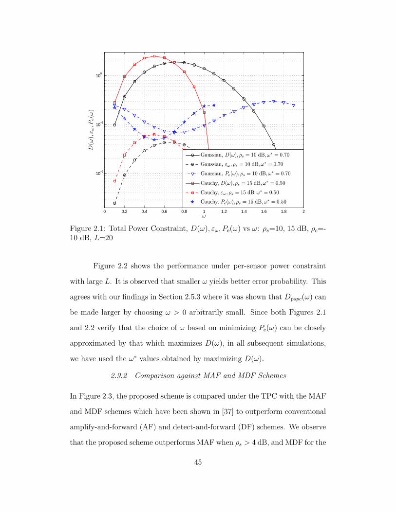
0 0.2 0.4 0.6 0.8 1 1.2 1.4 1.6 1.8 2
10−2
10−1
100
ω
D(ω
),ε
ω,P
e(ω
)
Gaussian, D(ω), ρs = 10 dB, ω∗ = 0.70
Gaussian, εω, ρs = 10 dB, ω∗ = 0.70
Gaussian, Pe(ω), ρs = 10 dB, ω∗ = 0.70
Cauchy, D(ω), ρs = 15 dB, ω∗ = 0.50
Cauchy, εω, ρs = 15 dB, ω∗ = 0.50
Cauchy, Pe(ω), ρs = 15 dB, ω∗ = 0.50
Figure 2.1: Total Power Constraint, D(ω), εω, Pe(ω) vs ω: ρs=10, 15 dB, ρc=-10 dB, L=20
Figure 2.2 shows the performance under per-sensor power constraint
with large L. It is observed that smaller ω yields better error probability. This
agrees with our findings in Section 2.5.3 where it was shown that Dpspc(ω) can
be made larger by choosing ω > 0 arbitrarily small. Since both Figures 2.1
and 2.2 verify that the choice of ω based on minimizing Pe(ω) can be closely
approximated by that which maximizes D(ω), in all subsequent simulations,
we have used the ω∗ values obtained by maximizing D(ω).
2.9.2 Comparison against MAF and MDF Schemes
In Figure 2.3, the proposed scheme is compared under the TPC with the MAF
and MDF schemes which have been shown in [37] to outperform conventional
amplify-and-forward (AF) and detect-and-forward (DF) schemes. We observe
that the proposed scheme outperforms MAF when ρs > 4 dB, and MDF for the
45
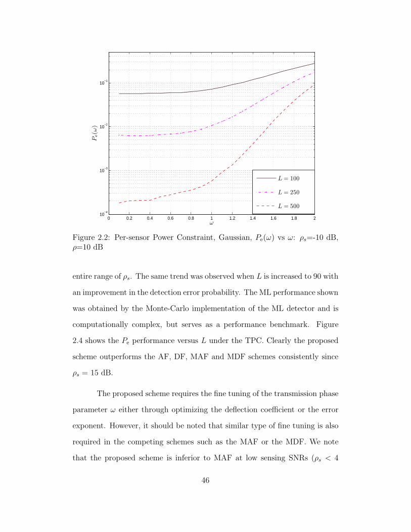
0 0.2 0.4 0.6 0.8 1 1.2 1.4 1.6 1.8 210
−4
10−3
10−2
10−1
ω
Pe(ω
)
L = 100
L = 250
L = 500
Figure 2.2: Per-sensor Power Constraint, Gaussian, Pe(ω) vs ω: ρs=-10 dB,ρ=10 dB
entire range of ρs. The same trend was observed when L is increased to 90 with
an improvement in the detection error probability. The ML performance shown
was obtained by the Monte-Carlo implementation of the ML detector and is
computationally complex, but serves as a performance benchmark. Figure
2.4 shows the Pe performance versus L under the TPC. Clearly the proposed
scheme outperforms the AF, DF, MAF and MDF schemes consistently since
ρs = 15 dB.
The proposed scheme requires the fine tuning of the transmission phase
parameter ω either through optimizing the deflection coefficient or the error
exponent. However, it should be noted that similar type of fine tuning is also
required in the competing schemes such as the MAF or the MDF. We note
that the proposed scheme is inferior to MAF at low sensing SNRs (ρs < 4
46
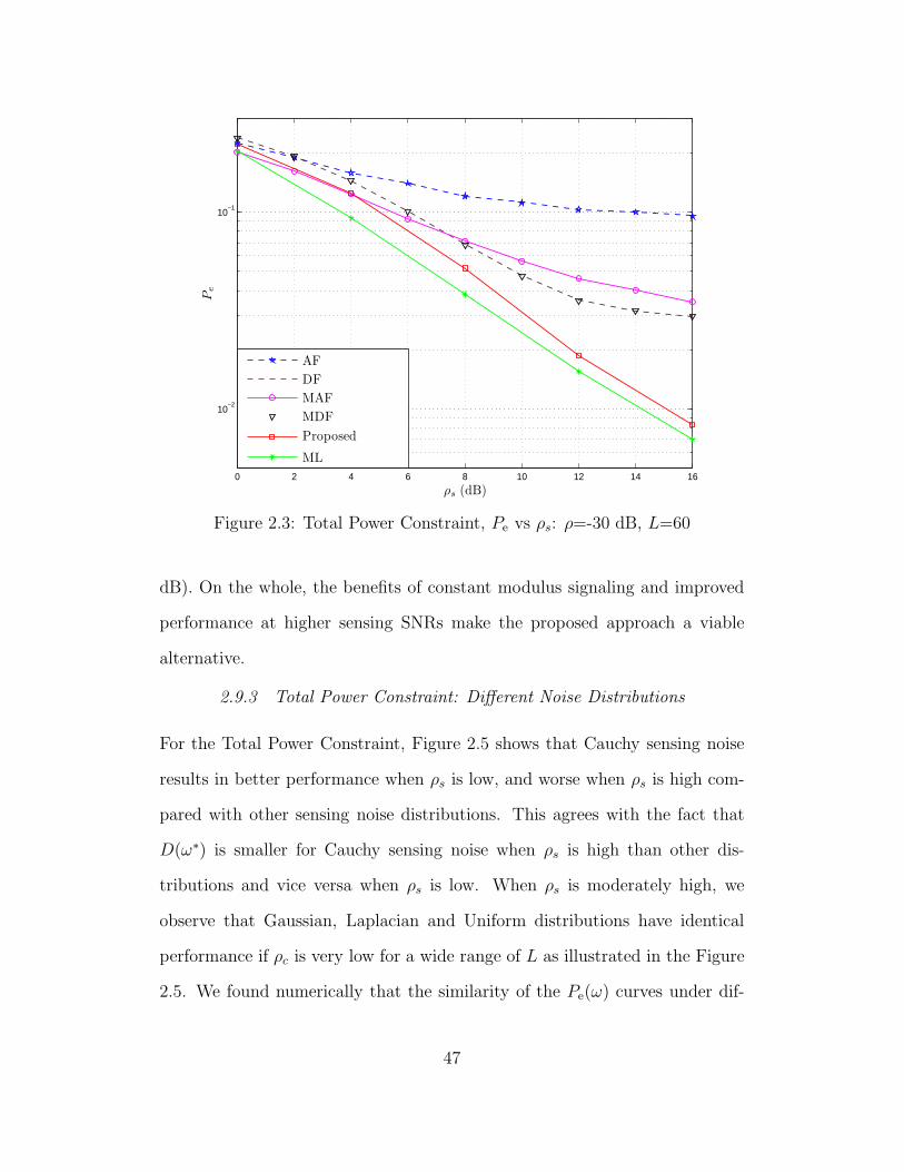
0 2 4 6 8 10 12 14 16
10−2
10−1
ρs (dB)
Pe
AF
DF
MAF
MDF
Proposed
ML
Figure 2.3: Total Power Constraint, Pe vs ρs: ρ=-30 dB, L=60
dB). On the whole, the benefits of constant modulus signaling and improved
performance at higher sensing SNRs make the proposed approach a viable
alternative.
2.9.3 Total Power Constraint: Different Noise Distributions
For the Total Power Constraint, Figure 2.5 shows that Cauchy sensing noise
results in better performance when ρs is low, and worse when ρs is high com-
pared with other sensing noise distributions. This agrees with the fact that
D(ω∗) is smaller for Cauchy sensing noise when ρs is high than other dis-
tributions and vice versa when ρs is low. When ρs is moderately high, we
observe that Gaussian, Laplacian and Uniform distributions have identical
performance if ρc is very low for a wide range of L as illustrated in the Figure
2.5. We found numerically that the similarity of the Pe(ω) curves under dif-
47
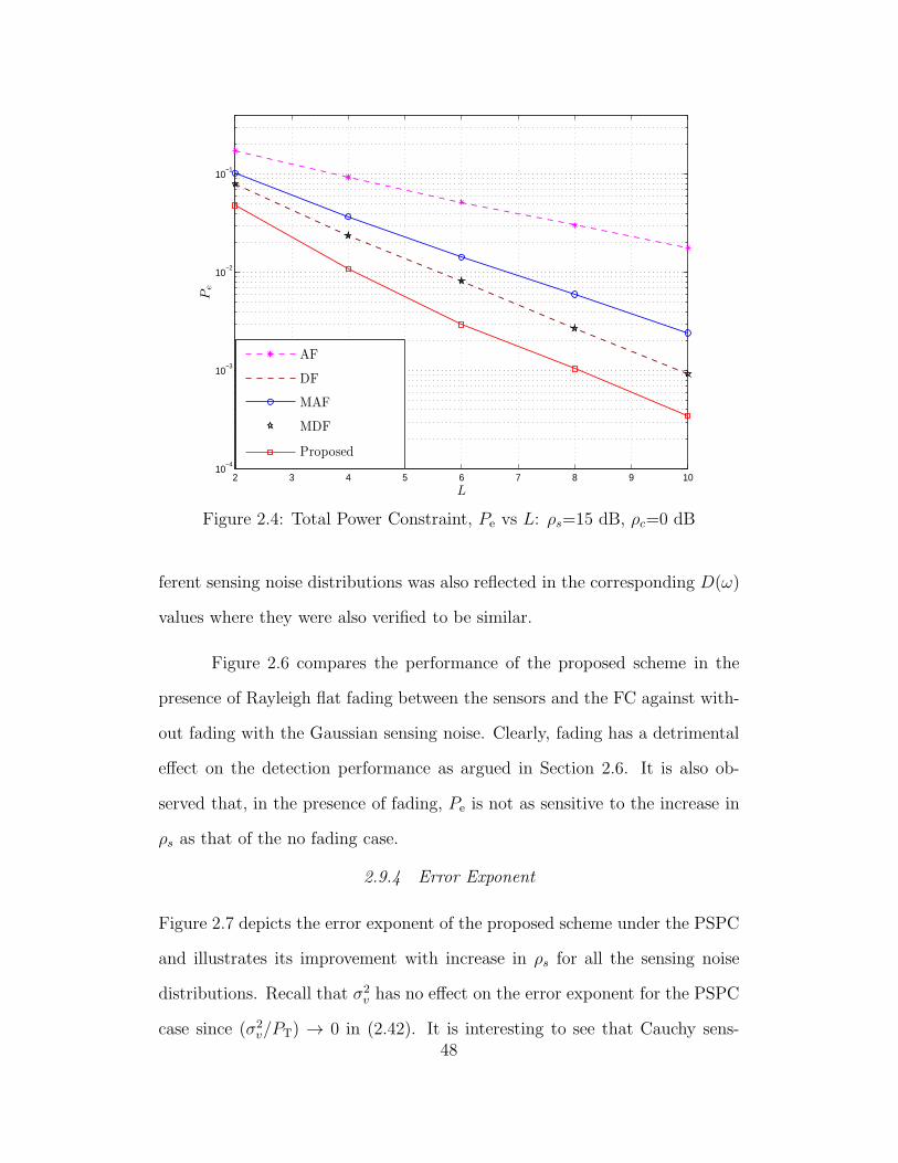
2 3 4 5 6 7 8 9 1010
−4
10−3
10−2
10−1
L
Pe
AF
DF
MAF
MDF
Proposed
Figure 2.4: Total Power Constraint, Pe vs L: ρs=15 dB, ρc=0 dB
ferent sensing noise distributions was also reflected in the corresponding D(ω)
values where they were also verified to be similar.
Figure 2.6 compares the performance of the proposed scheme in the
presence of Rayleigh flat fading between the sensors and the FC against with-
out fading with the Gaussian sensing noise. Clearly, fading has a detrimental
effect on the detection performance as argued in Section 2.6. It is also ob-
served that, in the presence of fading, Pe is not as sensitive to the increase in
ρs as that of the no fading case.
2.9.4 Error Exponent
Figure 2.7 depicts the error exponent of the proposed scheme under the PSPC
and illustrates its improvement with increase in ρs for all the sensing noise
distributions. Recall that σ2v has no effect on the error exponent for the PSPC
case since (σ2v/PT) → 0 in (2.42). It is interesting to see that Cauchy sens-
48
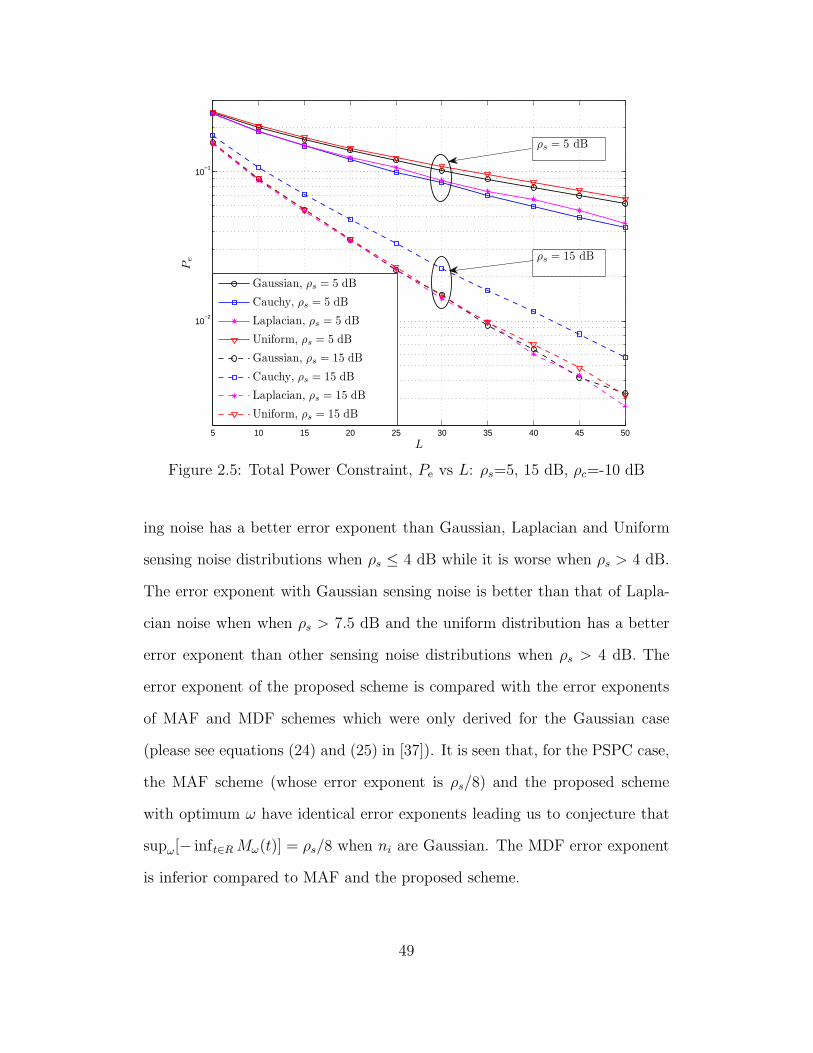
5 10 15 20 25 30 35 40 45 50
10−2
10−1
L
Pe
Gaussian, ρs = 5 dB
Cauchy, ρs = 5 dB
Laplacian, ρs = 5 dB
Uniform, ρs = 5 dB
Gaussian, ρs = 15 dB
Cauchy, ρs = 15 dB
Laplacian, ρs = 15 dB
Uniform, ρs = 15 dB
ρs = 15 dB
ρs = 5 dB
Figure 2.5: Total Power Constraint, Pe vs L: ρs=5, 15 dB, ρc=-10 dB
ing noise has a better error exponent than Gaussian, Laplacian and Uniform
sensing noise distributions when ρs ≤ 4 dB while it is worse when ρs > 4 dB.
The error exponent with Gaussian sensing noise is better than that of Lapla-
cian noise when when ρs > 7.5 dB and the uniform distribution has a better
error exponent than other sensing noise distributions when ρs > 4 dB. The
error exponent of the proposed scheme is compared with the error exponents
of MAF and MDF schemes which were only derived for the Gaussian case
(please see equations (24) and (25) in [37]). It is seen that, for the PSPC case,
the MAF scheme (whose error exponent is ρs/8) and the proposed scheme
with optimum ω have identical error exponents leading us to conjecture that
supω[− inft∈R Mω(t)] = ρs/8 when ni are Gaussian. The MDF error exponent
is inferior compared to MAF and the proposed scheme.
49
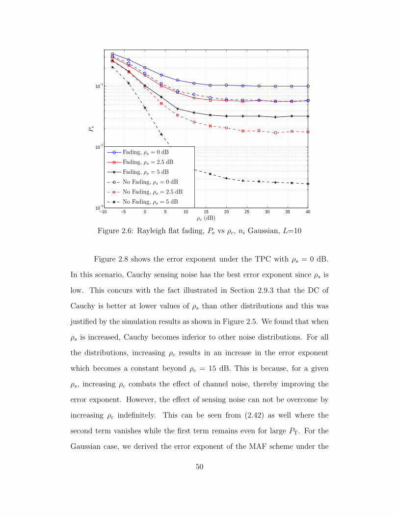
−10 −5 0 5 10 15 20 25 30 35 4010
−3
10−2
10−1
ρc (dB)
Pe
Fading, ρs = 0 dB
Fading, ρs = 2.5 dB
Fading, ρs = 5 dB
No Fading, ρs = 0 dB
No Fading, ρs = 2.5 dB
No Fading, ρs = 5 dB
Figure 2.6: Rayleigh flat fading, Pe vs ρc, ni Gaussian, L=10
Figure 2.8 shows the error exponent under the TPC with ρs = 0 dB.
In this scenario, Cauchy sensing noise has the best error exponent since ρs is
low. This concurs with the fact illustrated in Section 2.9.3 that the DC of
Cauchy is better at lower values of ρs than other distributions and this was
justified by the simulation results as shown in Figure 2.5. We found that when
ρs is increased, Cauchy becomes inferior to other noise distributions. For all
the distributions, increasing ρc results in an increase in the error exponent
which becomes a constant beyond ρc = 15 dB. This is because, for a given
ρs, increasing ρc combats the effect of channel noise, thereby improving the
error exponent. However, the effect of sensing noise can not be overcome by
increasing ρc indefinitely. This can be seen from (2.42) as well where the
second term vanishes while the first term remains even for large PT. For the
Gaussian case, we derived the error exponent of the MAF scheme under the
50
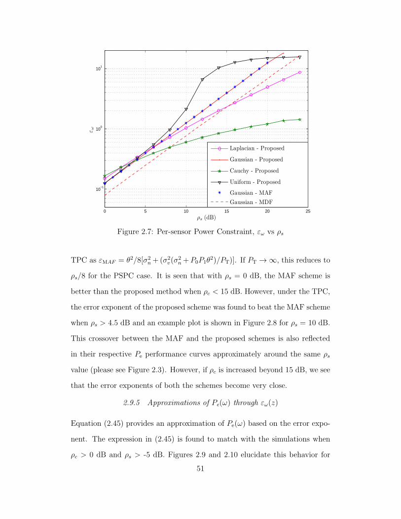
0 5 10 15 20 25
10−1
100
101
ρs (dB)
εω
Laplacian - Proposed
Gaussian - Proposed
Cauchy - Proposed
Uniform - Proposed
Gaussian - MAF
Gaussian - MDF
Figure 2.7: Per-sensor Power Constraint, εω vs ρs
TPC as εMAF = θ2/8[σ2n + (σ2
v(σ2n +P0P1θ
2)/PT)]. If PT → ∞, this reduces to
ρs/8 for the PSPC case. It is seen that with ρs = 0 dB, the MAF scheme is
better than the proposed method when ρc < 15 dB. However, under the TPC,
the error exponent of the proposed scheme was found to beat the MAF scheme
when ρs > 4.5 dB and an example plot is shown in Figure 2.8 for ρs = 10 dB.
This crossover between the MAF and the proposed schemes is also reflected
in their respective Pe performance curves approximately around the same ρs
value (please see Figure 2.3). However, if ρc is increased beyond 15 dB, we see
that the error exponents of both the schemes become very close.
2.9.5 Approximations of Pe(ω) through εω(z)
Equation (2.45) provides an approximation of Pe(ω) based on the error expo-
nent. The expression in (2.45) is found to match with the simulations when
ρc > 0 dB and ρs > -5 dB. Figures 2.9 and 2.10 elucidate this behavior for
51
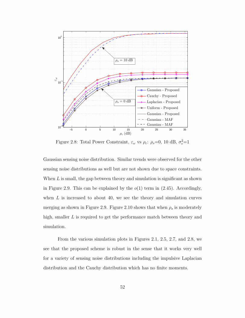
−5 0 5 10 15 20 25 30 3510
−2
10−1
100
ρc (dB)
εω
Gaussian - Proposed
Cauchy - Proposed
Laplacian - Proposed
Uniform - Proposed
Gaussian - Proposed
Gaussian - MAF
Gaussian - MAF
ρs = 10 dB
ρs = 0 dB
Figure 2.8: Total Power Constraint, εω vs ρc: ρs=0, 10 dB, σ2v=1
Gaussian sensing noise distribution. Similar trends were observed for the other
sensing noise distributions as well but are not shown due to space constraints.
When L is small, the gap between theory and simulation is significant as shown
in Figure 2.9. This can be explained by the o(1) term in (2.45). Accordingly,
when L is increased to about 40, we see the theory and simulation curves
merging as shown in Figure 2.9. Figure 2.10 shows that when ρs is moderately
high, smaller L is required to get the performance match between theory and
simulation.
From the various simulation plots in Figures 2.1, 2.5, 2.7, and 2.8, we
see that the proposed scheme is robust in the sense that it works very well
for a variety of sensing noise distributions including the impulsive Laplacian
distribution and the Cauchy distribution which has no finite moments.
52
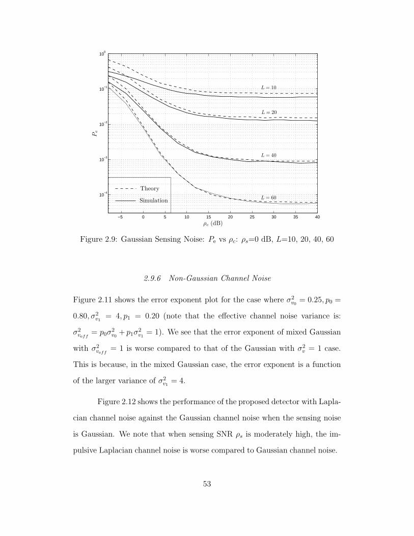
−5 0 5 10 15 20 25 30 35 40
10−4
10−3
10−2
10−1
100
ρc (dB)
Pe
L = 60
L = 40
L = 20
L = 10
Theory
Simulation
Figure 2.9: Gaussian Sensing Noise: Pe vs ρc: ρs=0 dB, L=10, 20, 40, 60
2.9.6 Non-Gaussian Channel Noise
Figure 2.11 shows the error exponent plot for the case where σ2v0
= 0.25, p0 =
0.80, σ2v1
= 4, p1 = 0.20 (note that the effective channel noise variance is:
σ2veff
= p0σ2v0+ p1σ
2v1
= 1). We see that the error exponent of mixed Gaussian
with σ2veff
= 1 is worse compared to that of the Gaussian with σ2v = 1 case.
This is because, in the mixed Gaussian case, the error exponent is a function
of the larger variance of σ2v1
= 4.
Figure 2.12 shows the performance of the proposed detector with Lapla-
cian channel noise against the Gaussian channel noise when the sensing noise
is Gaussian. We note that when sensing SNR ρs is moderately high, the im-
pulsive Laplacian channel noise is worse compared to Gaussian channel noise.
53
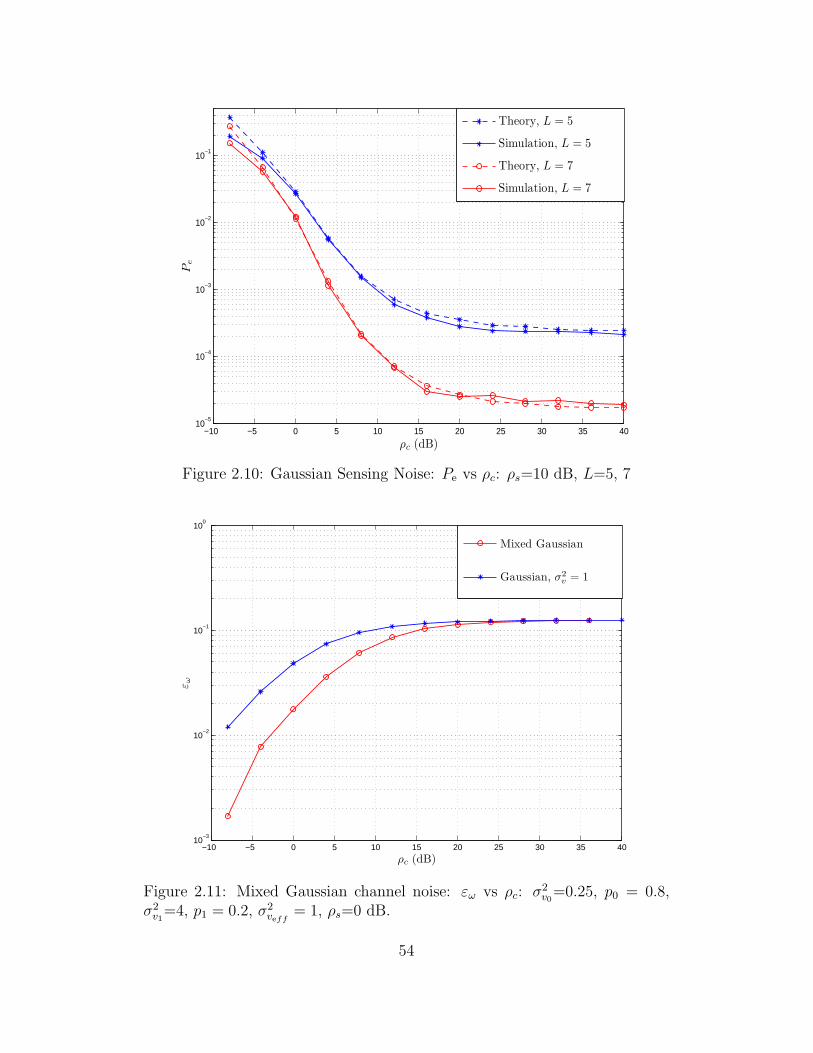
−10 −5 0 5 10 15 20 25 30 35 4010
−5
10−4
10−3
10−2
10−1
ρc (dB)
Pe
Theory, L = 5
Simulation, L = 5
Theory, L = 7
Simulation, L = 7
Figure 2.10: Gaussian Sensing Noise: Pe vs ρc: ρs=10 dB, L=5, 7
−10 −5 0 5 10 15 20 25 30 35 4010
−3
10−2
10−1
100
ρc (dB)
εω
Mixed Gaussian
Gaussian, σ2v
= 1
Figure 2.11: Mixed Gaussian channel noise: εω vs ρc: σ2v0=0.25, p0 = 0.8,
σ2v1=4, p1 = 0.2, σ2
veff= 1, ρs=0 dB.
54
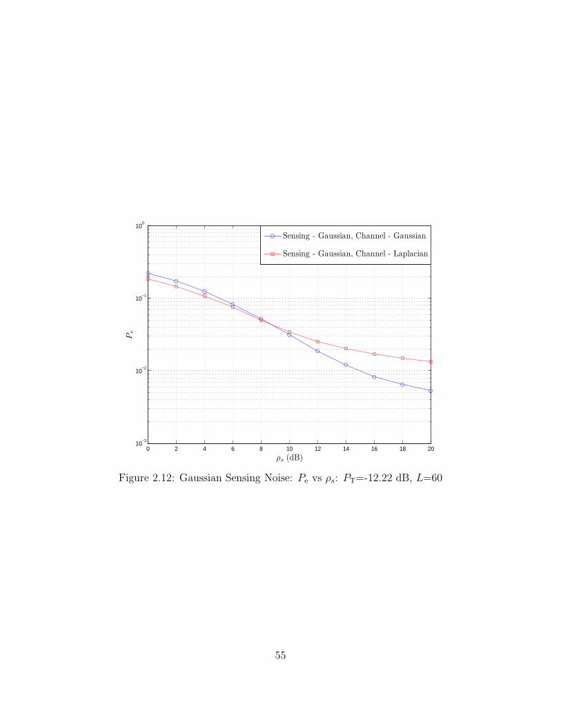
0 2 4 6 8 10 12 14 16 18 2010
−3
10−2
10−1
100
ρs (dB)
Pe
Sensing - Gaussian, Channel - Gaussian
Sensing - Gaussian, Channel - Laplacian
Figure 2.12: Gaussian Sensing Noise: Pe vs ρs: PT=-12.22 dB, L=60
55
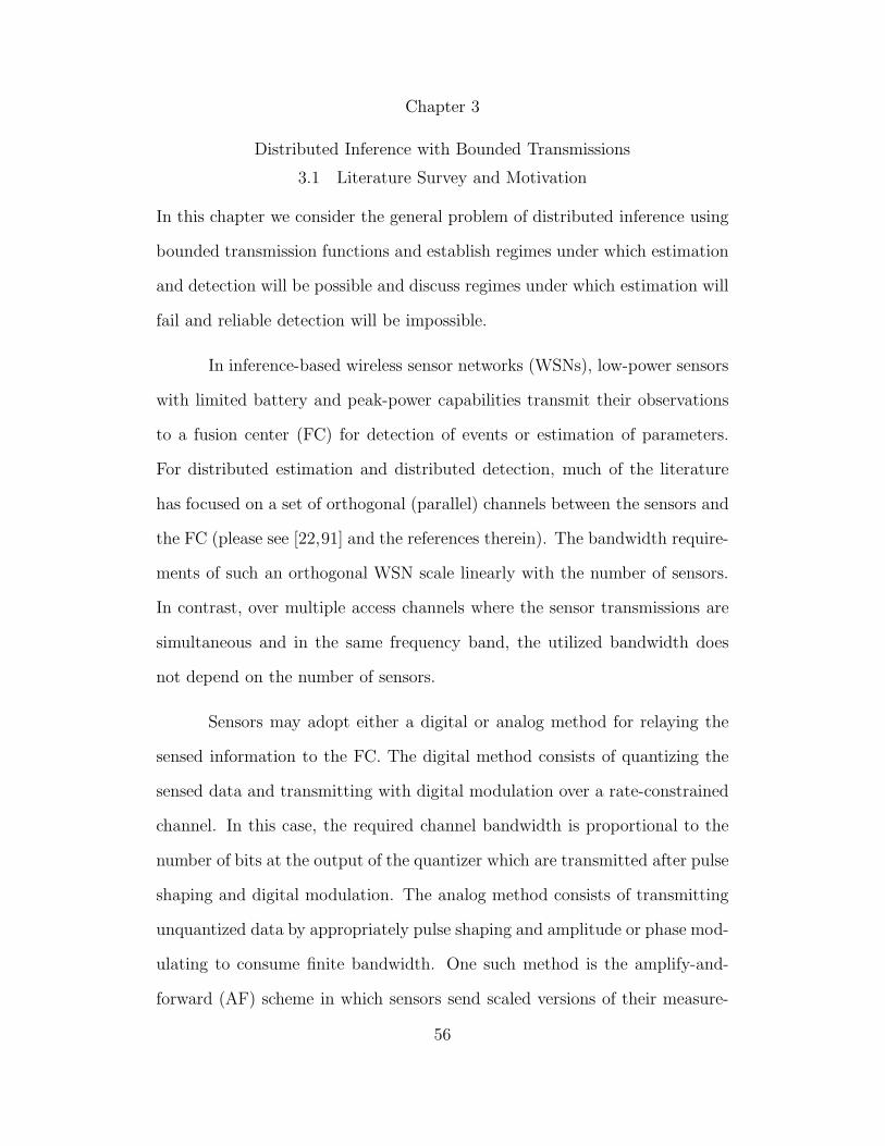
Chapter 3
Distributed Inference with Bounded Transmissions
3.1 Literature Survey and Motivation
In this chapter we consider the general problem of distributed inference using
bounded transmission functions and establish regimes under which estimation
and detection will be possible and discuss regimes under which estimation will
fail and reliable detection will be impossible.
In inference-based wireless sensor networks (WSNs), low-power sensors
with limited battery and peak-power capabilities transmit their observations
to a fusion center (FC) for detection of events or estimation of parameters.
For distributed estimation and distributed detection, much of the literature
has focused on a set of orthogonal (parallel) channels between the sensors and
the FC (please see [22,91] and the references therein). The bandwidth require-
ments of such an orthogonal WSN scale linearly with the number of sensors.
In contrast, over multiple access channels where the sensor transmissions are
simultaneous and in the same frequency band, the utilized bandwidth does
not depend on the number of sensors.
Sensors may adopt either a digital or analog method for relaying the
sensed information to the FC. The digital method consists of quantizing the
sensed data and transmitting with digital modulation over a rate-constrained
channel. In this case, the required channel bandwidth is proportional to the
number of bits at the output of the quantizer which are transmitted after pulse
shaping and digital modulation. The analog method consists of transmitting
unquantized data by appropriately pulse shaping and amplitude or phase mod-
ulating to consume finite bandwidth. One such method is the amplify-and-
forward (AF) scheme in which sensors send scaled versions of their measure-
56
ments to the FC. However, using the AF technique is not a viable option for
WSNs because it requires high transmission power when the values to be trans-
mitted are large [92]. Moreover, the linear transmit amplifier characteristics
required for AF are often very power-inefficient [93], requiring the study of the
effect of nonlinear transmissions on performance. Distributed systems which
employ the AF technique for transmission of the sensed data often assume
that the power amplifiers used are perfectly linear over the entire range of the
sensed observations. In practice, the amplifiers exhibit nonlinear behaviour
when the amplitude of the sensed data is relatively high [93–95]. Wireless
sensor networks have stringent power and bandwidth constraints, therefore
distributed schemes which use bounded instantaneous transmit power over
multiple access channels are highly desirable.
References [38,42–44,70,96,97] discuss distributed estimation over Gaus-
sian multiple access channels. In [38, 42], a distributed estimation scheme
where the sensor transmissions are phase-modulated to make constant mod-
ulus transmissions is considered. The estimator proposed in [38] is shown to
be strongly consistent for any symmetric sensing noise distribution when the
noise samples are i.i.d.. In [43, 44], the mean and variance of a signal embed-
ded in noise (not necessarily Gaussian) are estimated which are then used to
estimate the SNR of the signal. In all the above cases of [38, 42–44], the de-
sired constant modulus property is achieved by phase modulating the sensed
data before transmission. The authors in [98] discuss the effect of nonlinear
transmissions on the convergence speed of a consensus algorithm proposed for
a distributed average consensus problem.
References [36, 37, 99, 100] discuss distributed detection using constant
modulus transmissions over Gaussian multiple access channels for a binary
57
hypothesis testing problem. Inspired by the robustness of the estimation
scheme in [38], the authors in [99] and [100] proposed a distributed detection
scheme where the sensors transmit with constant modulus signals over a Gaus-
sian multiple access channel. Here again, the sensors transmit with constant
modulus transmissions whose phase varies linearly with the sensed data and
the performance is analysed using deflection coefficient and error exponent.
In [36] and [37], two schemes called modified amplify-and-forward (MAF)
and the modified detect-and-forward (MDF) are developed which generalize
and outperform the classic amplify-and-forward (AF) and detect-and-forward
(DF) approaches to distributed detection. It is shown that MAF outperforms
MDF when the number of sensors is large and the opposite conclusion is true
when the number of sensors is smaller. In both the DF and MDF schemes,
the sensors individually take a decision by quantizing the sensed measure-
ment and transmit the one bit information to the FC by BPSK modulation
and therefore the transmit power is always constant. Bounded transmission
schemes are highly desirable and practically viable for the power constrained
WSNs. In addition, bounded transmissions are robust to impulsive measure-
ments [38,42–44] which could happen for WSNs deployed in adverse conditions.
In this chapter, we are interested in studying the effect of general non-
linear transmissions (as opposed to the linear AF scheme) from the sensors to
the FC in a distributed inference framework. The sensors map their observa-
tions using a bounded function before transmission to constrain the transmit
power and these observations are transmitted to the FC over a Gaussian mul-
tiple access channel. Our emphasis in this Chapter is not so much to propose a
specific estimator or a detector, rather we want to focus on studying the impli-
cations of bounded transmission schemes on distributed inference in resource
58
constrained WSNs. Moreover, this work also studies the merits and demerits
of distributed schemes involving realistic, nonlinear amplifier characteristics.
We characterize the general conditions on the sensing noise statistics and the
nonlinear function under which consistent estimation and reliable detection
are possible. We also compare the bounded transmissions scheme with the
AF scheme and highlight the advantages and disadvantages of each other. We
show that if the measurement accuracy degrades progressively in the sense that
the sensing noise variance goes to infinity, bounded transmission is not useful
for distributed inference. On the other hand, it is shown that AF scheme does
not suffer from this issue. These conclusions are drawn by studying the fun-
damental metrics such the asymptotic variance and the deflection coefficient.
This chapter is organized as follows. In Section 3.2, the system model
is described with the total power constraint. In Section 3.3, the estimation
problem is described and the properties of the proposed estimator is stud-
ied. Optimization of AsV (ω) is considered in this section. In Section 3.3,
the detection problem is described and a quadratic detector is proposed. The
probability of error performance of the detector is analyzed and the optimiza-
tion of DC is studied in this section. The proposed scheme is compared against
the AF scheme in Section 3.2.4. Simulation results are provided in Section 3.4
which support the theoretical results.
3.2 Distributed Estimation with Bounded Transmissions3.2.1 System Model
Consider the sensing model, with L sensors,
xi = θ + σini i = 1, . . . , L (3.1)
where θ is an unknown real-valued parameter, ni is symmetric real-valued
noise with zero median (i.e., its probability density function (PDF) is sym-59
metric about zero), and xi is the measurement at the ith sensor. The noise
samples ni are assumed to be independent identically distributed (i.i.d.) but
not necessarily with finite mean or variance. We consider a setting where the
ith sensor transmits its measurement using a bounded function√ρf(xi) over
a Gaussian multiple access channel (please see Figure 3.1) so that the received
signal at the FC is given by
yL=
√ρ
L∑
i=1
f (xi) + v (3.2)
where ρ is a power scale factor and v is the additive Gaussian noise with
zero mean and variance σ2v . Parameter σi is a deterministic scale parameter
which makes the variance (when it exists) of the noise samples different for
each sensor depending on how they are distributed in space and how accurate
their measurements are. For instance, if the phenomenon quantified by θ
happens near a sensor, it is reasonable to expect that the variances of the
sensing noise would be higher compared to those that are farther. Moreover,
in case of WSNs operating in adverse conditions, the sensing noise ni could
be impulsive characterized by heavy tailed distributions [101]. We also point
out that the received signal at the FC as modeled in (3.2) is realistic if the
transmit amplifiers at the local sensors are nonlinear.
In this chapter, we study the consequences of the boundedness of f(·)
on performance. In particular, we assume that the transmit function f(x)
satisfies the following conditions.
Assumptions:
(A1): f(x) is differentiable such that 0 < f′
(x) ≤ d, ∀x ∈ R.
(A2): f(x) is bounded, supx∈R |f(x)| = c.
Note that the transmitted signal at the ith sensor has the instantaneous power
ρf 2(ωxi) and it is always constrained within ρc2, which does not suffer from60
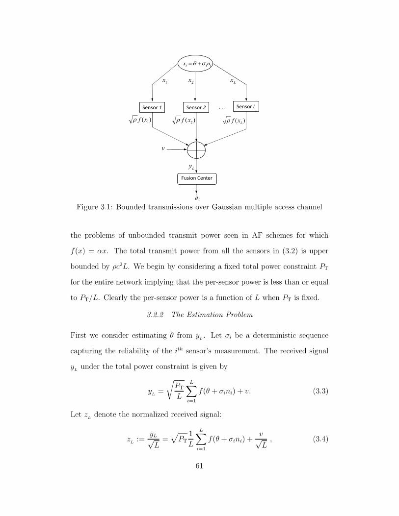
Fusion Center
. . . Sensor 1 Sensor 2 Sensor L
L
Ù
q
iii nx sq +=
1x 2x Lx
v
Ly
)( 1xfr )( 2xfr )( Lxfr
Figure 3.1: Bounded transmissions over Gaussian multiple access channel
the problems of unbounded transmit power seen in AF schemes for which
f(x) = αx. The total transmit power from all the sensors in (3.2) is upper
bounded by ρc2L. We begin by considering a fixed total power constraint PT
for the entire network implying that the per-sensor power is less than or equal
to PT/L. Clearly the per-sensor power is a function of L when PT is fixed.
3.2.2 The Estimation Problem
First we consider estimating θ from yL. Let σi be a deterministic sequence
capturing the reliability of the ith sensor’s measurement. The received signal
yLunder the total power constraint is given by
yL=
√PT
L
L∑
i=1
f(θ + σini) + v. (3.3)
Let zLdenote the normalized received signal:
zL:=
yL√L
=√
PT1
L
L∑
i=1
f(θ + σini) +v√L
, (3.4)
61
and define hω(θ) := L−1∑L
i=1 Eni[f(θ + σini)] where E(·) denotes expectation.
We now state an important result known as the Kolmogorov’s strong law of
large numbers [102, pp. 259] which handles the case of independent non-
identically distributed RVs, due to the fact that the σi are different.
Theorem 3.2.1. Let X1, X2, . . . , XL be a sequence of independent and
not necessarily identically distributed RVs. Let var[Xk] denote the variance
of Xk and XL = L−1∑L
k=1Xk denote the partial sum of the sequence. If∑∞
k=1 var[Xk]/k2 < ∞, then, XL − E[XL] → 0 almost surely as L → ∞.
Due to the law of large numbers in Theorem 3.2.1 we have
limL→∞
1
L
L∑
i=1
f(θ + σini) = hω(θ) (3.5)
where we use the fact that the variances var[f(θ + σini)] ≤ c2 are bounded.
Therefore, we have limL→∞ zL=
√PThω(θ). Due to the boundedness of f(·),
(3.5) holds regardless of the sensing noise distributions. Consider estimating
θ from,
θL = h−1ω
(zL√PT
), (3.6)
where zLis as given in (3.4). To recover θ uniquely from h−1
ω (·), we need
hω(θ) to be one-to-one in θ for which (A1) and (A2) are sufficient as shown
in Lemma 3.2.1.
Lemma 3.2.1. Let gσi(θ) := Eni
[f(θ + σini)] and suppose that the assump-
tions (A1) and (A2) hold. Then, hω(θ) is one-to-one in θ.
62
Proof. Differentiating gσi(θ) with respect to θ, we have
gσi(θ) =
∞∫
−∞
f(θ + σini)p(ni)dni ,
∂gσi(θ)
∂θ=
∞∫
−∞
∂f(θ + σini)
∂θp(ni)dni , (3.7)
> 0 , (3.8)
where we have applied Corollary 5.9 in [103, pp. 46] using assumptions (A1)
and (A2) to move the derivative inside the integral in (3.7). The last inequality
follows from the fact that convex combination of positive valued functions is
positive. Therefore, gσi(θ) is strictly an increasing function of θ. Since hω(θ)
is a convex combination of strictly increasing and differentiable functions, we
have h′
(θ) > 0, θ > 0. Therefore, hω(θ) is a strictly increasing function and
thus it is one-to-one in θ.
We now state a Lemma about a convergent sequence which will be used
in the sequel.
Lemma 3.2.2. Let ai be a converging sequence such that limi→∞ ai = a. Then,
limL→∞ L−1∑L
i=1 ai = a.
Proof. Please see [86, pp. 411].
An estimator θL is strongly consistent if θL converges to the true value
θ almost surely as L → ∞ [86]. Now we establish the strong consistency of
the class of estimators θL in (3.6) In Theorem 3.2.2.
Theorem 3.2.2. Let the assumptions (A1) and (A2) hold. Let σmax :=
maxi σi be finite. Then, the estimator θL in (3.6) is strongly consistent.
63
Proof. Since f(x) is a bounded function by assumption (A2), the Kolmogorov’s
condition∑∞
i=1 var[f((θ + σini)]/i2 ≤ ρ2c2π2/6 < ∞ is satisfied, therefore the
strong law of large numbers for the non-identically distributed random vari-
ables (RVs) is applicable and zL→ √
PThω(θ) almost surely. Since f′
(x) > 0
by assumption (A1), it follows from Lemma 3.2.1 that h(θ) is one-to-one in
θ. Due to the fact that θL is a continuous function of zL, θL → θ almost
surely [86, Thm 3.14] proving that the estimator in (3.6) is strongly consis-
tent.
On the other hand, if σi → ∞ as i → ∞, then the estimator in (3.6) is
not consistent and θ can not be estimated from zL. A more formal statement
is presented next as a theorem.
Theorem 3.2.3. Let the assumptions (A1) and (A2) hold and σi be a de-
terministic sequence such that σi → ∞ as i → ∞, then hω(θ) is independent
of θ.
Proof. First we note that due to assumption (A2), the variances var[f((θ +
σini)] are bounded. According to Kolmogorov’s strong law of large numbers
64
for non-identically distributed random variables, we have
hω(θ) = limL→∞
zL=√PT lim
L→∞
1
L
L∑
i=1
Enif(θ + σini) (3.9)
=√PT lim
L→∞
1
L
L∑
i=1
∞∫
−∞
f(θ + σini)p(ni)dni (3.10)
=√PT lim
L→∞
∞∫
−∞
1
L
L∑
i=1
f(θ + σini)p(ni)dni (3.11)
=√PT
∞∫
−∞
limL→∞
1
L
L∑
i=1
f(θ + σini)p(ni)dni (3.12)
=√PT
0∫
−∞
limL→∞
1
L
L∑
i=1
f(θ + σini)p(ni)dni
+√PT
∞∫
0
limL→∞
1
L
L∑
i=1
f(θ + σini)p(ni)dni (3.13)
=√PT
(−c2
2+
c12
)=
c1 − c22
(3.14)
for some c1 ≤ c, c2 ≤ c. We have exchanged the summation and expectation
in (3.10) to get (3.11). We have used assumption (A2) to apply bounded
convergence theorem [104, pp. 288] to move the limit in (3.11) inside the
integral as in (3.12). In (3.13), we have used Lemma 3.2.2 for the sequence
f(θ+ σini) along with the fact that f(x) converges to some constant as |x| →
∞ by the virtue of assumptions (A1) and (A2). Thus if σi → ∞, then
zL→ (c1− c2)/2 almost surely so that hω(θ) is independent of θ and therefore
θ can not be recovered from hω(θ) and the theorem is proved.
Theorem 3.2.3 indicates that if sensors use a bounded function to trans-
mit their measurements to the FC, there is a penalty incurred when the vari-
ance of the noise samples are going to infinity. When the noise samples are
very high in magnitude, the sensors will be transmitting the boundary values65
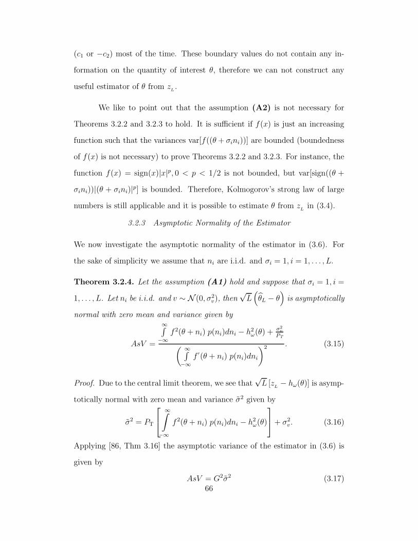
(c1 or −c2) most of the time. These boundary values do not contain any in-
formation on the quantity of interest θ, therefore we can not construct any
useful estimator of θ from zL.
We like to point out that the assumption (A2) is not necessary for
Theorems 3.2.2 and 3.2.3 to hold. It is sufficient if f(x) is just an increasing
function such that the variances var[f((θ+ σini))] are bounded (boundedness
of f(x) is not necessary) to prove Theorems 3.2.2 and 3.2.3. For instance, the
function f(x) = sign(x)|x|p, 0 < p < 1/2 is not bounded, but var[sign((θ +
σini))|(θ + σini)|p] is bounded. Therefore, Kolmogorov’s strong law of large
numbers is still applicable and it is possible to estimate θ from zLin (3.4).
3.2.3 Asymptotic Normality of the Estimator
We now investigate the asymptotic normality of the estimator in (3.6). For
the sake of simplicity we assume that ni are i.i.d. and σi = 1, i = 1, . . . , L.
Theorem 3.2.4. Let the assumption (A1) hold and suppose that σi = 1, i =
1, . . . , L. Let ni be i.i.d. and v ∼ N (0, σ2v), then
√L(θL − θ
)is asymptotically
normal with zero mean and variance given by
AsV =
∞∫−∞
f 2(θ + ni) p(ni)dni − h2ω(θ) +
σ2v
PT
( ∞∫−∞
f ′(θ + ni) p(ni)dni
)2 . (3.15)
Proof. Due to the central limit theorem, we see that√L [z
L− hω(θ)] is asymp-
totically normal with zero mean and variance σ2 given by
σ2 = PT
∞∫
−∞
f 2(θ + ni) p(ni)dni − h2ω(θ)
+ σ2
v . (3.16)
Applying [86, Thm 3.16] the asymptotic variance of the estimator in (3.6) is
given by
AsV = G2σ2 (3.17)66
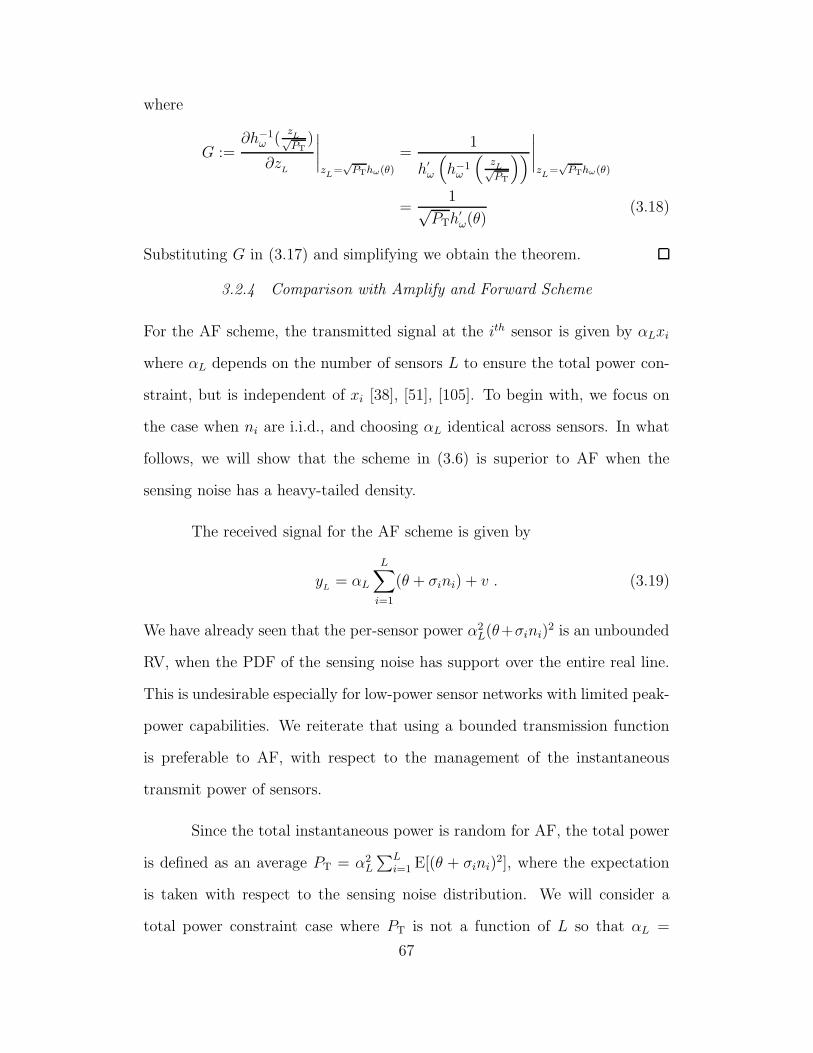
where
G :=∂h−1
ω (zL√PT
)
∂zL
∣∣∣∣zL=√PThω(θ)
=1
h′
ω
(h−1ω
(zL√PT
))∣∣∣∣zL=√PThω(θ)
=1√
PTh′
ω(θ)(3.18)
Substituting G in (3.17) and simplifying we obtain the theorem.
3.2.4 Comparison with Amplify and Forward Scheme
For the AF scheme, the transmitted signal at the ith sensor is given by αLxi
where αL depends on the number of sensors L to ensure the total power con-
straint, but is independent of xi [38], [51], [105]. To begin with, we focus on
the case when ni are i.i.d., and choosing αL identical across sensors. In what
follows, we will show that the scheme in (3.6) is superior to AF when the
sensing noise has a heavy-tailed density.
The received signal for the AF scheme is given by
yL= αL
L∑
i=1
(θ + σini) + v . (3.19)
We have already seen that the per-sensor power α2L(θ+σini)
2 is an unbounded
RV, when the PDF of the sensing noise has support over the entire real line.
This is undesirable especially for low-power sensor networks with limited peak-
power capabilities. We reiterate that using a bounded transmission function
is preferable to AF, with respect to the management of the instantaneous
transmit power of sensors.
Since the total instantaneous power is random for AF, the total power
is defined as an average PT = α2L
∑Li=1 E[(θ + σini)
2], where the expectation
is taken with respect to the sensing noise distribution. We will consider a
total power constraint case where PT is not a function of L so that αL =
67
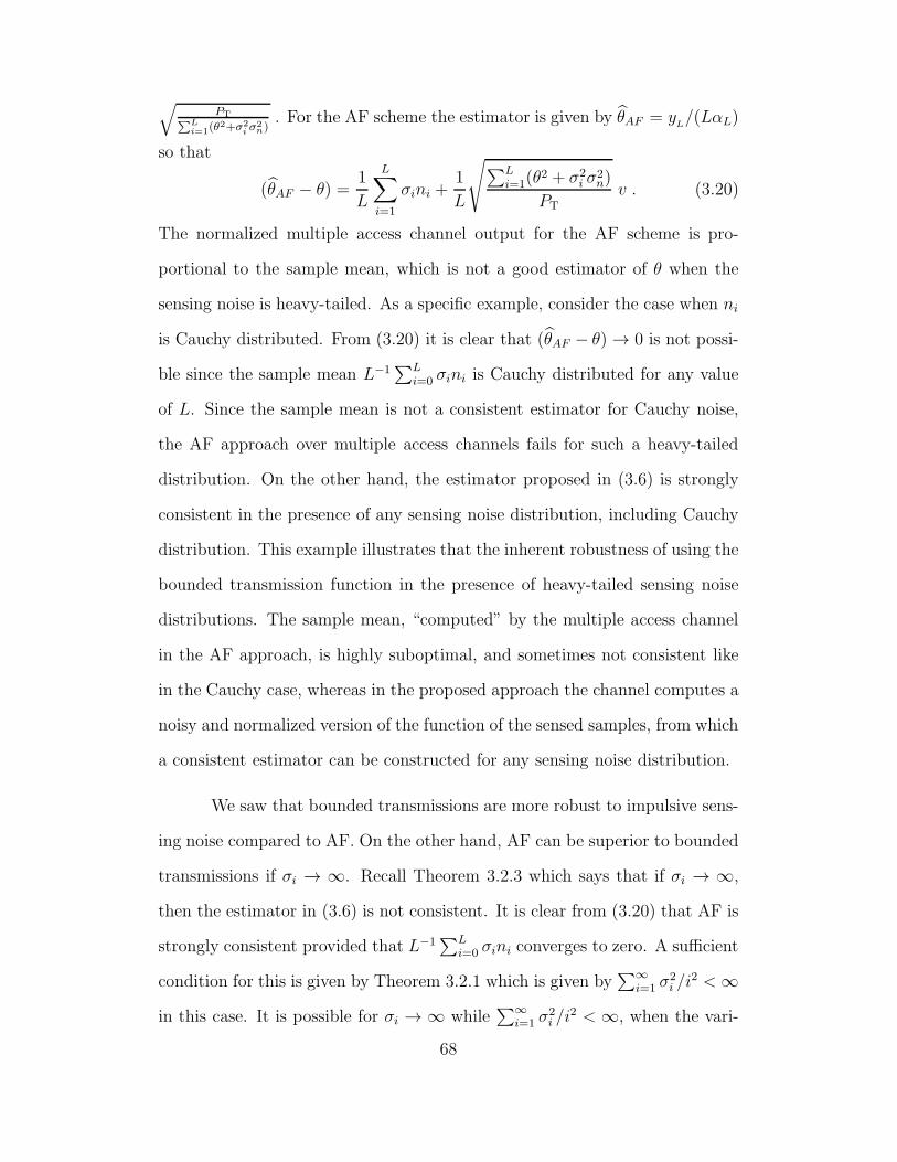
√PT∑L
i=1(θ2+σ2
i σ2n)
. For the AF scheme the estimator is given by θAF = yL/(LαL)
so that
(θAF − θ) =1
L
L∑
i=1
σini +1
L
√∑Li=1(θ
2 + σ2i σ
2n)
PTv . (3.20)
The normalized multiple access channel output for the AF scheme is pro-
portional to the sample mean, which is not a good estimator of θ when the
sensing noise is heavy-tailed. As a specific example, consider the case when ni
is Cauchy distributed. From (3.20) it is clear that (θAF − θ) → 0 is not possi-
ble since the sample mean L−1∑L
i=0 σini is Cauchy distributed for any value
of L. Since the sample mean is not a consistent estimator for Cauchy noise,
the AF approach over multiple access channels fails for such a heavy-tailed
distribution. On the other hand, the estimator proposed in (3.6) is strongly
consistent in the presence of any sensing noise distribution, including Cauchy
distribution. This example illustrates that the inherent robustness of using the
bounded transmission function in the presence of heavy-tailed sensing noise
distributions. The sample mean, “computed” by the multiple access channel
in the AF approach, is highly suboptimal, and sometimes not consistent like
in the Cauchy case, whereas in the proposed approach the channel computes a
noisy and normalized version of the function of the sensed samples, from which
a consistent estimator can be constructed for any sensing noise distribution.
We saw that bounded transmissions are more robust to impulsive sens-
ing noise compared to AF. On the other hand, AF can be superior to bounded
transmissions if σi → ∞. Recall Theorem 3.2.3 which says that if σi → ∞,
then the estimator in (3.6) is not consistent. It is clear from (3.20) that AF is
strongly consistent provided that L−1∑L
i=0 σini converges to zero. A sufficient
condition for this is given by Theorem 3.2.1 which is given by∑∞
i=1 σ2i /i
2 < ∞
in this case. It is possible for σi → ∞ while∑∞
i=1 σ2i /i
2 < ∞, when the vari-
68
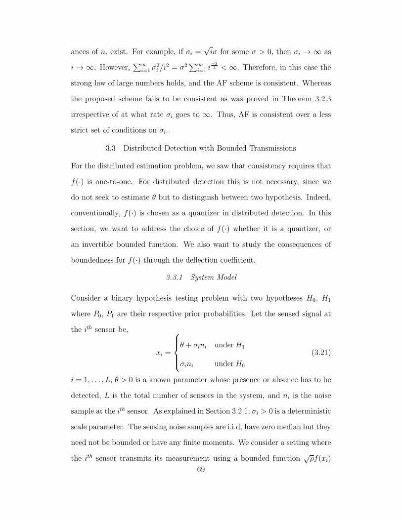
ances of ni exist. For example, if σi =√iσ for some σ > 0, then σi → ∞ as
i → ∞. However,∑∞
i=1 σ2i /i
2 = σ2∑∞
i=1 i−3
2 < ∞. Therefore, in this case the
strong law of large numbers holds, and the AF scheme is consistent. Whereas
the proposed scheme fails to be consistent as was proved in Theorem 3.2.3
irrespective of at what rate σi goes to ∞. Thus, AF is consistent over a less
strict set of conditions on σi.
3.3 Distributed Detection with Bounded Transmissions
For the distributed estimation problem, we saw that consistency requires that
f(·) is one-to-one. For distributed detection this is not necessary, since we
do not seek to estimate θ but to distinguish between two hypothesis. Indeed,
conventionally, f(·) is chosen as a quantizer in distributed detection. In this
section, we want to address the choice of f(·) whether it is a quantizer, or
an invertible bounded function. We also want to study the consequences of
boundedness for f(·) through the deflection coefficient.
3.3.1 System Model
Consider a binary hypothesis testing problem with two hypotheses H0, H1
where P0, P1 are their respective prior probabilities. Let the sensed signal at
the ith sensor be,
xi =
θ + σini underH1
σini underH0
(3.21)
i = 1, . . . , L, θ > 0 is a known parameter whose presence or absence has to be
detected, L is the total number of sensors in the system, and ni is the noise
sample at the ith sensor. As explained in Section 3.2.1, σi > 0 is a deterministic
scale parameter. The sensing noise samples are i.i.d, have zero median but they
need not be bounded or have any finite moments. We consider a setting where
the ith sensor transmits its measurement using a bounded function√ρf(xi)
69
over a Gaussian multiple access channel so that the received signal at the FC
is given by (3.2) where ρ is a power scale factor and f(x) satisfies the same
conditions as in Section 3.2.1, and v ∼ N (0, σ2v) is the additive channel noise.
Note that the power at each sensor is upper bounded by ρc2. We also assume
that the total power ρc2L for the entire network is constrained to PT.
3.3.2 The Detection Problem
The received signal yLunder the total power constraint can be written as
yL=
√PT
L
L∑
i=1
f (xi) + v . (3.22)
With the received signal in (3.22), the FC has to decide which hypothesis
is true. It is well known that the optimal decision rule under the Bayesian
formulation is given by:
p(yL|H1)
p(yL|H0)
H1
≷H0
P0
P1(3.23)
where p(yL|Hi), is the conditional probability density function of y
Lwhen the
hypothesis Hi, i ∈ {0, 1}, is true.
3.3.3 Probability of Error
The PDFs of yLin (3.23) under the hypothesis Hi involve (L+1) convolutions
and are not tractable in general. Let Pe be the probability of error at the FC:
Pe = P0 Pr [error|H0] + P1 Pr [error|H1] (3.24)
where Pr [error|Hi] is the error probability when Hi is true. Since Pe is not
straightforward to evaluate, we will study a surrogate metric called the deflec-
tion coefficient (DC) to identify regimes where reliable detection is possible.
The DC, depends only on the system model in (3.22), and does not depend
on any detector. As we are considering a general transmission scheme at the
local sensors, and Pe is not tractable, it is more insightful to study the DC.70
3.3.4 Deflection Coefficient and its Optimization
We will now define and use the deflection coefficient which reflects the output-
signal-to-noise-ratio and widely used in optimizing detectors [79–82]. The DC
is defined as,
D :=1
L
|E[yL|H1]− E[y
L|H0]|2
var[yL|H0]
. (3.25)
When σi is a deterministic sequence, the DC for the system in (3.22)
is given by
DL =
L−1
L∑
i=1
∞∫
−∞
[f(θ + σini)− f(σini)]p(ni)dni
2
L−1
L∑
i=1
∞∫
−∞
f 2(σini)p(ni)dni −
∞∫
−∞
f(σini)p(ni)dni
2+
σ2v
PT
.
(3.26)
We now study the conditions on the sequence σi for limL→∞DL= 0. When
this asymptotic DC is zero, the interpretation is that reliable detection is
not possible. The following result establishes that if σi goes to infinity, the
asymptotic DC is zero.
Theorem 3.3.1. Let σi be a deterministic sequence such that limi→∞ σi = ∞,
suppose that the assumptions (A1) and (A2) hold. Then, limL→∞DL= 0.
Proof. Clearly the denominator of (3.26) is bounded between (σ2v/PT) and
(c2 + σ2v/PT). Therefore, it suffices to show that the numerator goes to 0 as
71
L → ∞. Consider
limL→∞
DL= lim
L→∞
1
L
L∑
i=1
∞∫
−∞
[f(θ + σini)− f(σini)]p(ni)dni (3.27)
=
∞∫
−∞
limL→∞
1
L
L∑
i=1
[f(θ + σini)− f(σini)]p(ni)dni (3.28)
=
0∫
−∞
limL→∞
1
L
L∑
i=1
[f(θ + σini)− f(σini)]p(ni)dni
+
∞∫
0
limL→∞
1
L
L∑
i=1
[f(θ + σini)− f(σini)]p(ni)dni (3.29)
=(−c2
2+
c22
)+(c12− c1
2
)= 0 (3.30)
for some c1 ≤ c, c2 ≤ c and we have used assumption (A2) to apply bounded
convergence theorem [104, pp. 288] to move the limit in (3.27) inside the
integral as in (3.28). In (3.29), we have used Lemma 3.2.2 for the sequences
f(θ+σini) and f(σini) along with the fact that f(x) converges to some constant
as |x| → ∞ by the virtue of assumptions (A1) and (A2). Thus if σi → ∞,
then limL→∞DL= 0.
Theorem 3.3.1 indicates that if sensors use a bounded function to trans-
mit their measurements to the FC, there is a penalty incurred when the vari-
ance of the noise samples are very high. When the noise samples are very high
in magnitude, the sensors will be transmitting the boundary values of f(x),
i.e., c1 or −c2 most of the time. These boundary values do not contain any
information about the signal θ to be detected when H1 is true. Hence it is not
possible to distinguish between the hypothesis H1 and H0 and accordingly we
have the asymptotic DC equal to 0.
However, if σi are bounded, then we can show that limL→∞DL> 0
which is done next.72
Theorem 3.3.2. Let σmax := maxi σi be finite and suppose that the assump-
tions (A1) and (A2) hold. Then, limL→∞DL> 0.
Proof. Let gσi(θ) :=
∞∫−∞
[f(θ+σini)−f(σini)]p(ni)dni. To show limL→∞DL>
0, it suffices to show that gσi(θ) > 0, ∀θ > 0 for some i. Using the assumption
(A1) we have,
gσi(θ) =
∞∫
−∞
[f(θ + σini)− f(σini)]p(ni)dni ,
∂gσi(θ)
∂θ=
∞∫
−∞
∂f(θ + σini)
∂θp(ni)dni , (3.31)
> 0 , (3.32)
where we have applied Corollary 5.9 in [103, pp. 46] using assumptions (A1)
and (A2) to move the derivative in (3.31) inside the integral. The last inequal-
ity follows from the fact that convex combination of positive valued functions
is positive. Therefore, gσi(θ) is strictly an increasing function of θ. When
θ = 0, clearly gσi(0) = 0 and together with the fact that ∂g
σi(θ)/∂θ > 0,
∀θ > 0, we have gσi(θ) > 0, ∀θ > 0.
Theorem 3.3.2 says that if the deterministic σi are bounded, then the
asymptotic DC is strictly positive which means that reliable detection is pos-
sible in this regime.
Next we will prove that for the DC to be greater than zero, we do
not need f(x) to be a differentiable or strictly increasing. In the following
theorem we prove that DL> 0 for an uniform quantizer with bounded number
of quantization levels.
73
Theorem 3.3.3. Let σmax := maxi σi be finite and suppose that f(x) is a
uniform quantizer with M levels such that
f(x) =
k∆ , (k − 12)∆ ≤ x < (k + 1
2)∆ ,
K∆ , x ≥ (K + 12)∆ ,
−K∆ , x ≤ −(K + 12)∆
(3.33)
where k = −K,−(K − 1), . . . , 0, . . . , (K − 1), K, M = 2K + 1, ∆ = 2xmax/M
and xmax is the saturation point of the finite level quantizer. Suppose that ni
has infinite support. Then, DL> 0.
Proof. Let gσi(θ) :=
∞∫−∞
[f(θ + σini) − f(σini)]p(ni)dni. To show DL> 0, it
suffices to show that gσi(θ) > 0, ∀θ > 0. Note that the function f(x) in (3.33)
74
is non-decreasing, i.e., f(x)− f(y) ≥ 0, ∀x ≥ y. Consider
gσi(θ) =
∞∫
−∞
[f(θ + σini)− f(σini)]p(ni)dni (3.34)
=1
σi
∞∫
−∞
[f(θ + vi)− f(vi)]p(vi)dvi (3.35)
=1
σi
−[(K+ 1
2)∆+θ]∫
−∞
[f(θ + vi)− f(vi)]p(vi)dvi
+1
σi
(K+ 1
2)∆∫
−[(K+ 1
2)∆+θ]
[f(θ + vi)− f(vi)]p(vi)dvi
+1
σi
∞∫
(K+ 1
2)∆
[f(θ + vi)− f(vi)]p(vi)dvi (3.36)
≥ 1
σi
(K+ 1
2)∆∫
−[(K+ 1
2)∆+θ]
[f(θ + vi)− f(vi)]p(vi)dvi (3.37)
=1
σi
K∑
k=−K
(k+ 1
2)∆∫
[(k− 1
2)∆−θ]
∆p(vi)dvi (3.38)
> 0 (3.39)
where in (3.34) we substituted vi = σini to get (3.35). The inequality in
(3.39) follows from the fact that ∆ > 0 and vi has infinite support (since ni
has infinite support so that vi = σini has infinite support as well). When
θ = 0, clearly gσi(0) = 0 and therefore, we have D
L> 0, ∀θ > 0.
Theorem 3.3.3 can in fact be proved for non-uniform quantizer as long
as M ≥ 2 and ni has infinite support.
We would ideally like to find the f(x) that maximizes the DC in (3.26)
but this is not tractable. However, when θ is small, and channel noise is neg-75
ligible, we have a closed form expression for f(x) through the locally optimal
detection strategy. We now briefly discuss the use of nonlinear functions in
the context of locally optimal detection.
3.3.5 Locally Optimal Detection
A detector is said to be locally optimal (most powerful) if it is better than
any other detector in the sense of minimizing the probability of error for very
small values of θ (please see [101] for more details). The problem of designing
optimum detectors in the presence of additive noise has a long history in
the statistical signal processing literature [101]. Usually the sensing noise
corrupting the signal is assumed to be Gaussian. However there are situations
when the noise is impulsive, which are characterized by symmetric alpha stable
distributions [101]. In such scenarios, linear detector is not necessarily optimal,
and therefore nonlinear functions are applied on the sensed observations to
minimize the impact of impulsive sensing noise distributions with heavy tails.
In [101], it is shown that for a given sensing noise distribution p(n), the
nonlinear function f(x) that would be locally optimal is given by
f(x) = −p′
(x)
p(x). (3.40)
One may be interested in the inverse problem that given a nonlinear function
f(x), for which sensing noise distribution, it would be locally optimal. From
(3.40) it is easy to answer this question. We have,
p(x) = Ce−
x∫−∞
f(y)dy
. (3.41)
Here the p(x) obtained from (3.41) should be a valid PDF satisfying p(x) ≥ 0
and∞∫
−∞p(x)dx = 1. For example, if f(x) = tanh(x), we get p(x) = πsech(x) =
2πe−x/(1+e−2x). The sech(x) distribution behaves like the heavy-tailed Lapla-
cian distribution when x is relatively high. It is interesting to note that tanh(x)76
behaves like the hard clipper non-linearity [101] which is a bounded function
and is locally optimal for Laplacian noise distribution. In fact, a closer look
at (3.40) reveals that if p(x) behaves like an exponential density (for rela-
tively large x), then the f(x) that would be locally optimal would behave like
a constant (for relatively large x). This shows that the family of increasing
bounded functions are locally optimal for the family of heavy tailed sensing
noise distributions. When n is Gaussian, bounded f(x) is no longer optimal
as it is well known that f(x) = x is optimal for Gaussian sensing noise. We
will illustrate this in the Simulations section.
3.4 Simulations
In this section, we corroborate our analytical results through Monte Carlo sim-
ulations for both the distributed estimation and distributed detection prob-
lems. In all of the simulations we have assumed σi = 1, i = 1, . . . , L.
3.4.1 Distributed Estimation Performance
In Figure 3.2 we chose f(x) = tanh(ωx), ω > 0 is a scale parameter. Here we
compare AsV (ω) and Lvar(θL− θ) versus ω under the total power constraint
for various distributions on the sensing noise ni. We observe that the variance
of the asymptotic distribution, AsV (ω) and the normalized limiting variance
Lvar(θL− θ) are closer to each other when L is sufficiently large. However if
L is smaller, we see that there is significant difference between AsV (ω) and
Lvar(θL−θ) as illustrated in Figure 3.3. This is due to the finite sample effect,
and when L is increased, Lvar(θL− θ) decreases to converge its limiting value
of AsV (ω). In Figure 3.4, we compare AsV (ω) and Lvar(θL− θ) versus L.
Clearly in all cases, as L increases the Lvar(θL− θ) approaches its limiting
values of AsV (ω).
77
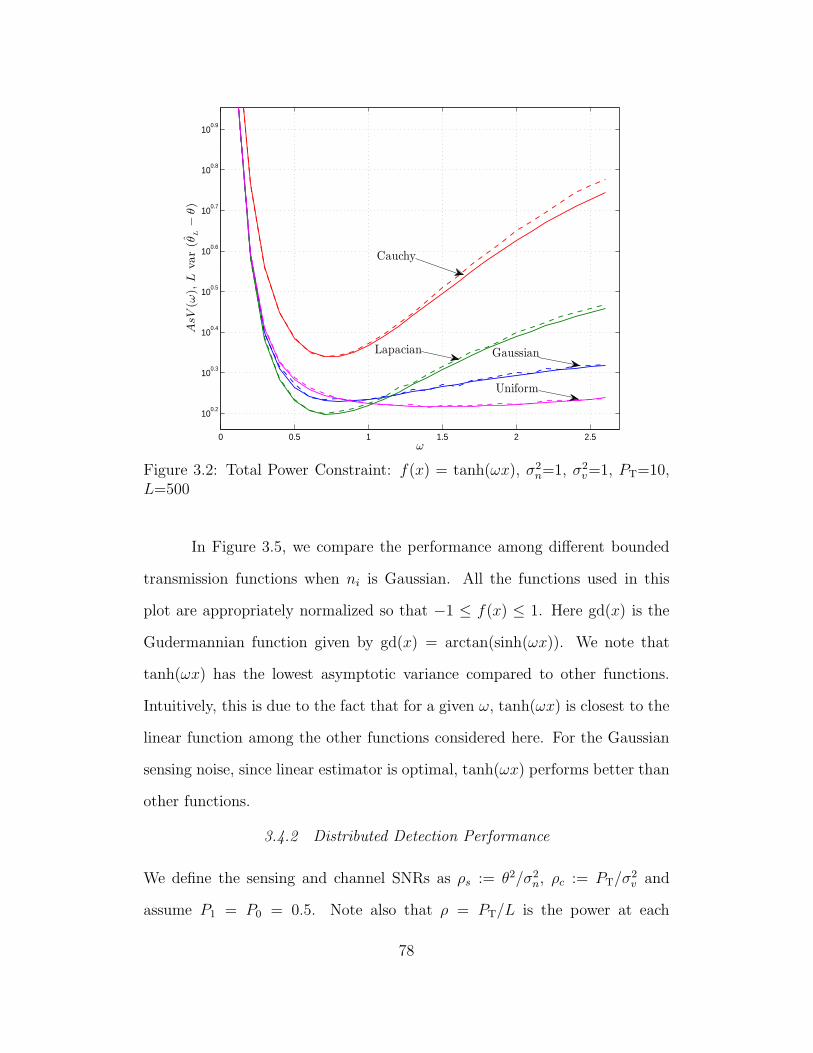
0 0.5 1 1.5 2 2.5
100.2
100.3
100.4
100.5
100.6
100.7
100.8
100.9
ω
AsV
(ω),
Lvar
(θL−
θ)
Lapacian Gaussian
Uniform
Cauchy
Figure 3.2: Total Power Constraint: f(x) = tanh(ωx), σ2n=1, σ2
v=1, PT=10,L=500
In Figure 3.5, we compare the performance among different bounded
transmission functions when ni is Gaussian. All the functions used in this
plot are appropriately normalized so that −1 ≤ f(x) ≤ 1. Here gd(x) is the
Gudermannian function given by gd(x) = arctan(sinh(ωx)). We note that
tanh(ωx) has the lowest asymptotic variance compared to other functions.
Intuitively, this is due to the fact that for a given ω, tanh(ωx) is closest to the
linear function among the other functions considered here. For the Gaussian
sensing noise, since linear estimator is optimal, tanh(ωx) performs better than
other functions.
3.4.2 Distributed Detection Performance
We define the sensing and channel SNRs as ρs := θ2/σ2n, ρc := PT/σ
2v and
assume P1 = P0 = 0.5. Note also that ρ = PT/L is the power at each
78
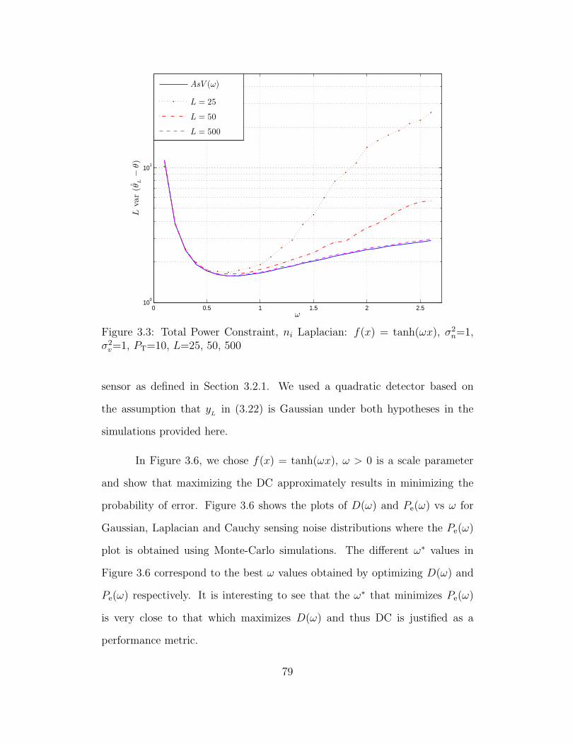
0 0.5 1 1.5 2 2.510
0
101
ω
Lvar
(θL−
θ)
AsV (ω)
L = 25
L = 50
L = 500
Figure 3.3: Total Power Constraint, ni Laplacian: f(x) = tanh(ωx), σ2n=1,
σ2v=1, PT=10, L=25, 50, 500
sensor as defined in Section 3.2.1. We used a quadratic detector based on
the assumption that yLin (3.22) is Gaussian under both hypotheses in the
simulations provided here.
In Figure 3.6, we chose f(x) = tanh(ωx), ω > 0 is a scale parameter
and show that maximizing the DC approximately results in minimizing the
probability of error. Figure 3.6 shows the plots of D(ω) and Pe(ω) vs ω for
Gaussian, Laplacian and Cauchy sensing noise distributions where the Pe(ω)
plot is obtained using Monte-Carlo simulations. The different ω∗ values in
Figure 3.6 correspond to the best ω values obtained by optimizing D(ω) and
Pe(ω) respectively. It is interesting to see that the ω∗ that minimizes Pe(ω)
is very close to that which maximizes D(ω) and thus DC is justified as a
performance metric.
79
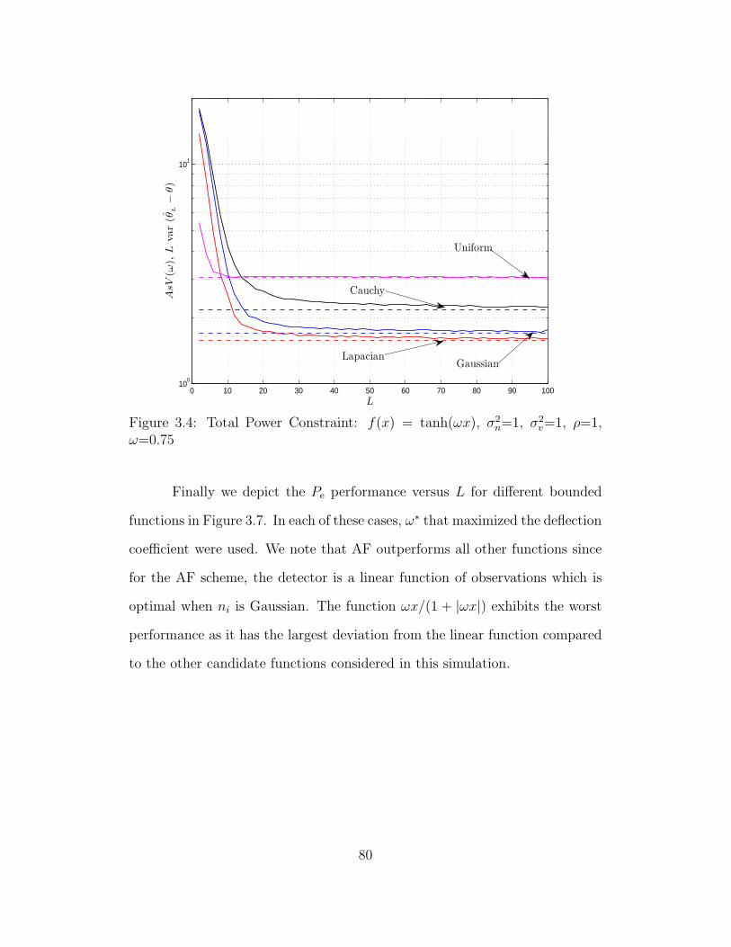
0 10 20 30 40 50 60 70 80 90 10010
0
101
L
AsV
(ω),
Lvar
(θL−
θ)
Uniform
GaussianLapacian
Cauchy
Figure 3.4: Total Power Constraint: f(x) = tanh(ωx), σ2n=1, σ2
v=1, ρ=1,ω=0.75
Finally we depict the Pe performance versus L for different bounded
functions in Figure 3.7. In each of these cases, ω∗ that maximized the deflection
coefficient were used. We note that AF outperforms all other functions since
for the AF scheme, the detector is a linear function of observations which is
optimal when ni is Gaussian. The function ωx/(1 + |ωx|) exhibits the worst
performance as it has the largest deviation from the linear function compared
to the other candidate functions considered in this simulation.
80

0 0.5 1 1.5 2 2.5
100.2
100.3
100.4
100.5
100.6
100.7
100.8
100.9
ω
AsV
(ω),
Lvar
(θL−
θ)
2
πgd(π
2ωx) 2
πtan−1(π
2ωx) ωx
1+|ωx|
tanh(ωx)
Figure 3.5: Total Power Constraint, Different bounded functions: σ2n=1, σ2
v=1,PT=10, L=500
0 0.5 1 1.510
−3
10−2
10−1
ω
D(ω
),P
e(ω
)
Gaussian - Pe(ω), ω∗ = 0.25
Gaussian - D(ω), ω∗ = 0.25
Laplacian - D(ω), ω∗ = 0.25
Laplacian - Pe(ω), ω∗ = 0.25
Cauchy - D(ω), ω∗ = 0.25
Cauchy - Pe(ω), ω∗ = 0.25
Figure 3.6: Total Power Constraint, f(x) = tanh(ωx), D(ω) Pe(ω) versus ω,ρs = 10 dB, ρc = 3 dB, L=20
81
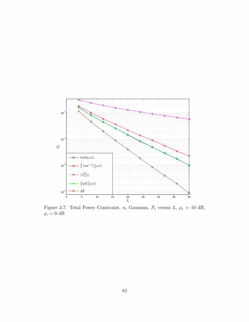
0 5 10 15 20 25 30 35 40
10−4
10−3
10−2
10−1
L
Pe
tanh(ωx)
2
πtan−1(π
2ωx)
ωx
1+|ωx|
2
πgd(π
2ωx)
AF
Figure 3.7: Total Power Constraint, ni Gaussian, Pe versus L, ρs = 10 dB,ρc = 0 dB
82
Chapter 4
Distributed Consensus with Bounded Transmissions
4.1 Literature Survey and Motivation
In this chapter, we consider the problem of estimating the average of sam-
ples measured at the nodes of a sensor network without a fusion center (fully
distributed network). Distributed computing has been a subject of extensive
research in the last two decades with a wide range of applications (see for
example [1, 2]). Originally, the purpose of distributed algorithms was to re-
duce the burden on a single processor and perform computationally large tasks
in a distributed manner on multiple processors which were physically wired.
With the recent interest in wireless sensor networks (WSNs), the focus has got
shifted to performing global computations with the data available locally at
each node of a WSN in a distributed manner. For example, the sensor nodes in
a WSN could measure information about a physical phenomenon of interest.
These measurements can be used for estimating unknown parameters of the
physical phenomenon (distributed estimation) or they can be used to make a
decision about the state of the physical phenomenon (distributed detection).
Wireless sensor networks (WSNs) without a fusion center have the ad-
vantages of robustness to node failures and they can function autonomously
without a central node controlling the entire network [2]. In such fully dis-
tributed networks, sensors collaborate with their neighbours by repeatedly
exchanging information locally to achieve a desired global objective. For ex-
ample, the sensors could come to an agreement on the sample average (or on a
global function) of initial measurements. This is called distributed consensus.
Distributed consensus algorithms have attracted significant interest in the re-
cent past and have found several applications in areas such as healthcare, envi-
83
ronmental monitoring, military and home appliances (please see [58–61,63–65]
and references therein). In this body of literature, it is often assumed that
a given node can obtain exact information of the state values of its neigh-
bours through local communications. This essentially means that the system
consumes theoretically unlimited energy and bandwidth. However, practical
WSNs are severely power limited and the available bandwidth is finite. More-
over, the main source of power consumption in a sensor is its transceiver [106].
Therefore, there is a need for consensus algorithms which work under strict
resource constraints of power and bandwidth imposed by the WSNs.
Sensors may adopt either a digital or analog method for transmitting
their information to their neighbours. Digital methods of transmissions may
be using low transmit power but require increased bandwidth especially when
the number of quantization levels is high. Distributed consensus algorithms
using quantized transmissions have been studied in [107–111]. The analog
method consists of transmitting unquantized data by appropriately pulse shap-
ing and amplitude or phase modulating to consume finite bandwidth. One such
method is the amplify-and-forward (AF) scheme in which sensors send scaled
versions of their measurements to their neighbours. However, using the AF
technique is not a viable option for WSNs because it requires high transmis-
sion power when the values to be transmitted are large [92]. Moreover, the
linear transmit amplifier characteristics required for AF are often very power-
inefficient [93], requiring the study of the effect of non-linear transmissions
on performance. In distributed systems which employ the AF technique for
transmission of the sensed data, it is often assumed that the power amplifiers
used are perfectly linear over the entire range of the sensed observations. In
84
practice, the amplifiers exhibit non-linear behaviour when the amplitude of
the sensed data is relatively high [93–95].
In this chapter, we propose a non-linear distributed consensus (NLC)
algorithm in which every sensor maps its state value through a bounded func-
tion before transmission to constrain the peak transmit power. Therefore the
magnitude of the transmitted signal at every node in every iteration is always
bounded, making it ideal for resource-constrained WSNs. In the presence
of communication noise, we prove that all the sensors employing the NLC
algorithm reach consensus to a finite random variable whose mean is the de-
sired sample average. We characterize the asymptotic performance by deriving
the asymptotic covariance matrix using results from stochastic approximation
theory. We show that using the NLC algorithm results in larger asymptotic
covariance compared to the linear consensus algorithm. Finally we explore
the performance of the proposed algorithm employing various bounded trans-
mission functions. Different from [65] which also considered consensus in the
presence of noisy transmissions, herein we analyse non-linear transmissions
and study the asymptotic covariance matrix and its dependence on the non-
linearity. Our work in this chapter also studies the merits and demerits of
distributed schemes involving realistic amplifier models with non-linear char-
acteristics such as the ones discussed in [93, 94].
The rest of this chapter is organized as follows. We begin by reviewing
some basics of network graph theory in Section 4.2. In Section 4.3, we describe
the system model and review the previous work on non-linear consensus. We
consider the NLC algorithm in the presence of noise in Section 4.4, and prove
that the sensors reach consensus to a random variable. In Section 4.5, we
85
present several simulation examples to study the performance of the proposed
algorithm.
Notations and Conventions
Vectors are denoted by boldface upper-case or lower-case letters and matrices
are denoted by boldface upper-case letters. max{a1, a2} denotes the maximum
of a1 and a2. diag[a1, a2, . . . , aN ] denotes an N ×N diagonal matrix whose
diagonal elements are given by a1, a2, . . . , aN . E[·] denotes the expectation
operator and I denotes the identity matrix. The symbol ‖ · ‖ denotes the l2
norm for real vectors and spectral norm for symmetric matrices. For a matrix
M, λi(M) denotes the ith smallest eigenvalue. The vector 1 denotes an N × 1
column vector of all ones, 1 = [1 1 . . . 1]T.
4.2 Review of Network Graph Theory
In this chapter, we model a sensor network as an undirected graph. In this
section, we provide a brief background on network graph theory which we will
use to derive our results. Consider an undirected graph G = (N,E) containing
a set of nodes N = {1, . . . , N} and a set of edges E. Nodes that communicate
with each other have an edge between them. We denote the set of neighbours
of node i by Ni, Ni = { j|{i, j} ∈ E} where {i, j} indicates an edge between
the nodes i and j [112]. A graph is connected if there exists at least one path
between every pair of nodes. We denote the number of neighbours of a node
i by di and dmax = maxi di. The graph structure is described by an N × N
symmetric matrix called the adjacency matrix A = {aij}, aij = 1 if {i, j} ∈ E.
The diagonal matrix D = diag[d1, d2, . . . , dN ] captures the degrees of all
the nodes in the network. The Laplacian matrix of the graph is given by
L = D−A.
86
The graph Laplacian characterises a number of useful properties of
the graph. The eigenvalues of L are non-negative and the number of zero
eigenvalues denotes the number of distinct components of the graph. When
the graph is connected, λ1(L) = 0, and λi(L) > 0, i ≥ 2, so that the rank of L
for a connected graph is N−1. The vector 1 is the eigenvector of L associated
with the eigenvalue 0, i.e, L1 = 0. The eigenvalue λ2(L) characterizes how
densely the graph is connected and the performance of consensus algorithms
depend on this eigenvalue [62].
4.3 System Model and Previous Work4.3.1 System Model
Consider a WSN withN sensor nodes each with an initial measurement xi(0) ∈
R. Measurements made at the sensor nodes are modeled as
xi(0) = θ + ni , i = 1, . . . , N (4.1)
where θ is an unknown real-valued parameter and ni is the sensing noise at
the ith sensor. The sample mean of these initial measurements in (4.1) is given
by
x =1
N
N∑
i=1
xi(0) . (4.2)
Let x be the estimate of the parameter θ to be computed by an iterative
distributed algorithm, in which each sensor communicates only with its neigh-
bours. If the states of all the sensor nodes converge to x, then the network is
said to have reached consensus on the sample average.
4.3.2 Previous Work
A commonly used iterative algorithm for distributed consensus can be written
as
87
xi(t+ 1) = xi(t)− α∑
j∈Ni
h(xi(t)− xij(t)) , (4.3)
where i = 1, . . . , N , t = 0, 1, 2, . . ., is the time index, xi(t + 1) is the updated
state value of sensor node i at time t+ 1, Ni is the set of neighbours of sensor
node i, xij(t), j ∈ Ni are the state values of the neighbours of sensor node i at
time t, and α is a constant step size. If h(·) is linear, then (4.3) is a linear dis-
tributed average-consensus (LDAC) algorithm [58,61,62]. In [58], it is proved
that if 0 < α < 2/λN(L), then xi(t) converges to x exponentially and (4.3) is
then called as the LDAC algorithm based on the Laplacian heuristic. If h(·)
is non-linear then the algorithm belongs to the class of non-linear distributed
average-consensus algorithms [60, 113–117]. In [60], the average consensus
problem is solved when h(x) in (4.3) is differentiable and odd. In [113], it
is illustrated that when h(x) in (4.3) is sin(x), faster convergence is possible
compared to the LDAC algorithm based on the Laplacian heuristic. In all
of these cases, xij(t) has to be transmitted to node i before it can apply the
function h(·) to get the new updated state value. Therefore, the transmit peak
power in (4.3) is determined by xi(t) and not necessarily bounded, even if h(·)
is bounded. Moreover, there is no communication noise assumed in all the
previous work on non-linear consensus.
4.4 Consensus with Bounded Transmissions and Communication Noise
In this work, we propose a distributed non-linear average consensus algorithm
in which every sensor maps its state value through a bounded function before
transmission to constrain the transmit power. Therefore the magnitude of the
transmitted signal at every node in every iteration is always bounded making
it ideal for resource-constrained WSNs.
88
In this section, we will study the NLC algorithm with communication
noise when sensors exchange information. Our approach is similar to, but
more general than [65] in that we analyse non-linear transmissions. Moreover,
unlike [65] we study the asymptotic covariance matrix of the state vector and
its dependence on the non-linearity. Unlike [113] and [60], we assume transmit
non-linearity which allows for bounded transmissions. Moreover, we consider
the presence of communication noise.
4.4.1 The NLC Algorithm with Communication Noise
Let each sensor map its state value at time t through the function h(x) before
transmission, and consider the following NLC algorithm with communication
noise:
xi(t+ 1) = xi(t)− α(t)∑
j∈Ni
[h(xi(t))− h(xij(t)) + nij(t)] , (4.4)
where i = 1, . . . , N, t = 0, 1, 2, . . ., is the time index. The value xi(t + 1) is
the state update of node i at time t + 1, xij(t) is the state value of the jth
neighbour of node i at time t and α(t) is a positive step size which will further
be assumed to satisfy assumption (A4) in the sequel. The node j transmits
its information xij(t) by mapping it through the function h(x), node i receives
a noisy version of h(xij(t)) and nij(t) is the noise associated with the reception
of h(xij(t)).
Note that the proposed scheme (4.4) is different from (4.3) in the fol-
lowing aspects. Firstly, in (4.3), xij(t) has to be transmitted which could
exhibit variation over a wide range of values if xi(0) has a large dynamic range
and hence (4.3) does not guarantee bounded transmission power. In contrast,
in the proposed scheme the non-linearity is applied before the state value is
transmitted so that the magnitude of the transmitted state value is always
89
constrained within the maximum value of h(x) irrespective of the range of
xi(t) and the realizations of noise nij(t). Finally, (4.4) involves communica-
tion noise while (4.3) does not. Thus the proposed scheme is more suited to
resource constrained WSNs when compared to (4.3).
The recursion in (4.4) can be written in vector form as
X(t+ 1) = X(t)− α(t) [Lh(X(t)) + n(t)] , (4.5)
where X(t) is state vector at time t given by X(t) = [x1(t) x2(t) . . . xN(t)]T,
and h : RN → RN such that h(X(t)) = [h(x1(t)) h(x2(t)) . . . h(xN (t))]T.
The vector n(t) captures the additive noise at N nodes contributed by their
respective neighbours and its ith component is given by
ni(t) = −∑
j∈Ni
nij(t) , 1 ≤ i ≤ N . (4.6)
Our model in (4.5) is more general than the linear consensus algorithm con-
sidered in [65] which is a special case of h(x) when it is linear. We make the
following assumptions on h(x), nij(t), α(t) and the graph:
Assumptions
(A1): The graph G is connected so that λ2(L) > 0.
(A2): The function h(·) is differentiable, and has a bounded derivative such
that 0 < h′
(x) ≤ c, for some c > 0.
(A3) Independent Noise Sequence: The channel noise {nij(t)}t≥0,1≤i,j≤N
is an independent sequence across time and space. It also satisfies
E[nij(t)] = 0, 1 ≤ i, j ≤ N, t ≥ 0, supi,j,t
E[n2ij(t)] ≤ σ2 < ∞. (4.7)
From (4.6) we have
E[n(t)] = 0 , ∀t , µ := supt
E[‖n(t)‖2] ≤ Ndmaxσ2 < ∞. (4.8)
90
Note that (4.8) is because of the fact that the number of neighbours of a given
node is upper bounded by dmax.
(A4) Decreasing Weight Sequence: The channel noise in (4.5) could
make the algorithm diverge. In order to control the variance growth rate of
the noise we need the following conditions on the sequence α(t):
α(t) > 0 ,
∞∑
t=0
α(t) = ∞ ,
∞∑
t=0
α2(t) < ∞ . (4.9)
Our primary motivation for considering non-linear transmissions is to
impose the realistic assumption of bounded peak per-sensor power by ensuring
that h(·) is bounded. However, as seen in (A2) this assumption is not needed
for our subsequent development as long as h′
(·) is bounded.
We will prove convergence and asymptotic normality result of the NLC
algorithm in (4.5). For the sake of clarity, we now present a result on the con-
vergence of a discrete time Markov process which will be used in establishing
convergence of the NLC algorithm in (4.5).
4.4.2 A Result on the Convergence of Discrete time Markov Processes
Let X = {X(t)}t≥0 be a discrete time vector Markov process on RN . The
generating operator L of X is defined as
LV (x) = E [V (X(t+ 1))|X(t) = x]− V (x) (4.10)
for functions V (x),x ∈ RN , provided that the conditional expectation exists.
Let B ⊂ RN and its complement be B′
= RN \ B. We now state the desired
result as a simplification of Theorem 2.7.1 in [118] (see also Theorem 1 in [65]).
Theorem 4.4.1. Let X be a discrete time vector Markov process with the
generator operator L as in (4.10). If there exists a potential function V (x) :
91
RN → R+, and B ⊂ RN with the following properties
V (x) > 0,x ∈ B′
, V (x) = 0, x ∈ B , (4.11)
LV (x) ≤ −γ(t)ϕ(x) +mg(t)[1 + V (x)] (4.12)
where m > 0, ϕ(x) is such that
ϕ(x) = 0,x ∈ B, ϕ(x) > 0,x ∈ B′
, (4.13)
and
γ(t) > 0, g(t) > 0,
∞∑
t=0
γ(t) = ∞,
∞∑
t=0
g(t) < ∞ , (4.14)
then, the discrete time vector Markov process X = {X(t)}t≥0 with arbitrary
initial distribution converges almost surely (a.s.) to the set B as t → ∞. That
is,
Pr
[limt→∞
infY∈B
‖X(t)−Y‖ = 0
]= 1. (4.15)
Intuitively, Theorem 4.4.1 indicates that if the one-step prediction error
of the Markov process evaluated at the potential function in (4.10) is bounded
as in (4.12) then it is possible to establish convergence of X(t).
To prove the a.s. convergence of the consensus algorithm in (4.5) using
Theorem 4.4.1, we define the consensus subspace B, the set of all vectors whose
entries are of equal value as,
B = {x ∈ RN |x = a1 , a ∈ R} . (4.16)
We are now ready to state the main result of Section 4.4.
92
Theorem 4.4.2. Let the assumptions (A1), (A3) and (A4) hold, and as-
sume h(x) is strictly increasing. Consider the NLC algorithm in (4.5) with the
initial state vector X(0) ∈ RN . Then, the state vector X(t) in (4.5) approaches
the consensus subspace B a.s., i.e.,
Pr
[limt→∞
infY∈B
‖X(t)−Y‖ = 0
]= 1. (4.17)
Proof. We will make use of Theorem 4.4.1 to prove (4.17). We will choose
an appropriate potential function V (x) that is non-negative which satisfies
equation (4.11). We will then prove that the generating operator L applied
on V (x) as in (4.10) can be upper bounded as in (4.12) with γ(t) = α(t), and
a ϕ(x) can be found that satisfies (4.13).
First we see that under the assumptions (A1), (A2) and the assump-
tion on h(x), the discrete time vector process {X(t)}t≥0 is Markov. Since L
is a positive semi-definite matrix, it has an eigenvalue decomposition (EVD)
given by L = UΣUT, where Σ is the diagonal matrix containing the eigen-
values of L in the increasing order, and U is a unitary matrix with 1 as its
first column vector which corresponds to the 0 eigenvalue. Define a posi-
tive semi-definite matrix M as a function of U such that M = UΛUT and
Λ = diag[0, 1, 1 , . . . , 1]. Let V (x) = xTMx, then the function V (x) is non-
negative since M is a positive semi-definite matrix by construction. Note that
x ∈ B is an eigenvector of M associated with the zero eigenvalue, therefore we
have
V (x) = 0,x ∈ B . (4.18)
Let x = xB + xB⊥ where xB is the orthogonal projection of x on B. When
x ∈ B′
, we have ‖xB⊥‖ > 0. Let x ∈ B′
and h(x) be as defined in (4.5). Then,93
h(x) = hB(x) + hB⊥(x), where hB⊥(x) is non-zero, i.e., ‖hB⊥(x)‖ > 0. Define
β := ‖hB⊥(x)‖2/‖xB⊥‖2, then β > 0, x ∈ B′
. Therefore, for any x ∈ B′
,
V (x) = xTMx = V (xB + xB⊥) = V (xB⊥)
≥ minxB⊥ 6=0
xTB⊥MxB⊥ = λ2(M)‖xB⊥‖2 > 0 , (4.19)
where the last inequality is due to λ2(L) > 0 by assumption (A1). The
equations (4.18) and (4.19) establish that the conditions in (4.11) in Theorem
4.4.1 are satisfied.
Now we will prove that (4.12) is satisfied as well. Towards this end,
consider LV (x) defined in (4.10),
LV (x) = E[X(t+ 1)TMX(t + 1)|X(t) = x
]− V (x), (4.20)
= E[(xT − α(t)
(h(x)TLT + n(t)T
))·
(Mx− α(t) (MLh(x) +Mn(t)))]− V (x) (4.21)
= −2α(t)[xTMLh(x)
]
+ α2(t)[h(x)TLTMLh(x) + E
[n(t)TMn(t)
]]. (4.22)
We get (4.22) by expanding (4.21) and taking the expectations and using the
fact that E[n(t)] = 0. Recall the EVDs of L and M from which we have
LM = ML = UΣUTUΛUT = UΣUT = L . (4.23)
Since λ2(M) = λN(M) = 1, we have
E[n(t)TMn(t)
]≤ E
[λN(M)‖n(t)‖2
]≤ µ, (4.24)
94
where the second inequality follows from (4.8) and the fact that λN(M) = 1.
Using (4.23) and (4.24) in (4.22), we get the following bound
LV (x) ≤ −2α(t)[xTLh(x)
]+ α2(t)
[h(x)TL2h(x) + µ
](4.25)
≤ −2α(t)[xTLh(x)
]+ α2(t)
[λ2N(L)β‖xB⊥‖2 + µ
](4.26)
≤ −2α(t)[xTLh(x)
]+ α2(t)
[βλ2N (L)
λ2(M)xTMx+ µ
](4.27)
≤ −2α(t)[xTLh(x)
]+mα2(t)
[1 + β2x
TMx]
(4.28)
≤ −α(t)ϕ(x) +mα2(t) [1 + V (x)] , (4.29)
where ϕ(x) := 2xTLh(x), m := max{βλ2N(L)/λ2(M), µ}, β2 := µ/m and
β2 ∈ (0, 1]. In (4.26), we have used the fact h(x)TL2h(x) ≤ λ2N(L)‖hB⊥(x)‖2
and ‖hB⊥(x)‖2 = β‖xB⊥‖2. In (4.27), we have used the fact that xTMx ≥
λ2(M)‖xB⊥‖2 due to (4.19). We will now prove that ϕ(x) in (4.29) satisfies
the equation (4.13) of Theorem 4.4.1.
Recall that L is the Laplacian matrix of the graph and that 1 is in
its null space, that is, L1 = 0. Whenever x ∈ B, i.e., x = a1, a ∈ R, then
h(x) = b1 for some b ∈ R. This implies Lh(a1) = Lb1 = 0. Therefore we
have ϕ(x) = 2xTLh(x) = 0, ∀x ∈ B.
To prove ϕ(x) > 0 when x ∈ B′
, consider ϕ(x) for a connected graph
with L of dimension N ×N ,
ϕ(x) = 2xTLh(x) (4.30)
= 2
[∑
j∈N1
(x1 − xj)h(x1) +∑
j∈N2
(x2 − xj)h(x2)
+ . . .+∑
j∈NN
(xN − xj)h(xN)
], (4.31)
where (4.31) follows from the structure of the symmetric matrix L (recall
L = D − A). Note that the ith summation in (4.31) corresponds to the ith
95
node. Now suppose that node i is connected to node j. Then there exists a
term (xi − xj)h(xi) in the summation corresponding to the ith node in (4.31),
and a term (xj − xi)h(xj) in the summation corresponding to the jth node in
(4.31). Both of these terms can be combined as (xi − xj)(h(xi) − h(xj)) and
this corresponds to the edge {i, j} ∈ E. Thus equation (4.31) can be written
as pairwise products enumerated over all the edges in the graph as follows
ϕ(x) = 2∑
{i,j}∈E(xi − xj)(h(xi)− h(xj)) . (4.32)
Since x ∈ B′
, ϕ(x) in (4.32) is positive due to the fact that h(x) is strictly
increasing so that there is at least one term in the sum which is strictly greater
than zero. Letting γ(t) = α(t), g(t) = α2(t) and by assumption (A4), we see
that the sequence α(t) in (4.29) satisfies (4.14). Thus all the conditions of
Theorem 4.4.1 are satisfied to yield (4.17).
Theorem 4.4.2 states that the sample paths of X(t) approach the con-
sensus subspace almost surely. We note that the assumption (A2) is not
necessary for Theorem 4.4.2 to hold. Instead we assumed h(x) is strictly in-
creasing (not necessarily differentiable) to prove Theorem 4.4.2. Now, like
in [65], we will prove the convergence of X(t) to a finite point in B in Theorem
4.4.3.
Theorem 4.4.3. Let the assumptions of Theorem 4.4.2 hold. Consider the
NLC algorithm in (4.5) with the initial state X(0) ∈ RN . Then, there exists a
finite real random variable θ∗ such that
Pr[limt→∞
X(t) = θ∗1]= 1. (4.33)
96
Proof. Let the average ofX(t) be x(t) = 1TX(t)/N . Since 1x(t) ∈ B, Theorem
4.4.2 implies,
Pr[limt→∞
‖X(t)− x(t)1‖ = 0]= 1 , (4.34)
where (4.34) follows from (4.17) since the infimum in (4.17) is achieved by
Y = x(t)1. Pre-multiplying (4.5) by 1T/N on both sides and noting that
1TLh(X(t)) = 0 we get,
x(t+ 1) = x(t)− v(t) (4.35)
= x(0)−∑
0≤k≤t
v(k) (4.36)
where v(t) = α(t)1Tn(t)/N . From assumption (A3), it follows that
E[v(t)] = 0,
∑
t≥0
E[v(t)]2 =∑
t≥0
α2(t)
N2E‖n(t)‖2 ≤ µ
N2
∑
t≥0
α2(t) < ∞
which implies
E[x(t + 1)]2 ≤ x2(0) +µ
N2
∑
t≥0
α2(t) , ∀t . (4.37)
Equation (4.37) implies that the sequence {x(t)}t≥0 is an L2 bounded mar-
tingale 1 and hence converges a.s. and in L2 to a finite random variable θ∗
(see [118, Theorem 2.6.1]). Therefore the theorem follows from (4.34).
It should be noted that the results in Theorems 4.4.2 and 4.4.3 are
similar to the results in [65], but we have proved it for a more general case of
which [65] is a special case when h(x) = x. In what follows, we present the
properties of the limiting random variable θ∗.1A sequence of random variables {y(t)}t≥0 is called as a martingale if for all t ≥ 0,
E [|y(t)|] < ∞ and E [y(t+ 1) | y(1) y(2) . . . y(t)] = y(t). The sequence {y(t)}t≥0 is an L2
bounded martingale if suptE[y2(t)
]< ∞ (see [119, pp. 110]).
97
4.4.3 Mean Square Error of NLC Algorithm
The Theorems 4.4.2 and 4.4.3 establish that the sensors reach consensus
asymptotically and converge a.s. to a finite random variable θ∗. We can
view θ∗ as an estimate of x. In the following theorem we characterize the
unbiasedness and means squared error (MSE) properties of θ∗. We define the
MSE of θ∗ as ξN= E[(θ∗ − x)2].
Theorem 4.4.4. Let θ∗ be the limiting random variable as in Theorem 4.4.3.
Then θ∗ is unbiased, E[θ∗] = x, and its MSE is bounded, ξN≤ µN−2
∑
t≥0
α2(t).
The proof is obtained by following the same steps of the Lemma 5
in [65].
We point out that with non-linear transmissions, we have obtained
the same bound on the MSE ξN
as that of the linear consensus algorithm
in [65]. It should be noted that µ ≤ Ndmaxσ2 from (4.8) which implies that
ξN≤ dmaxN
−1∑
t≥0 α2(t)σ2. Therefore, if dmax is finite for a large connected
network, we have limN→∞ ξN
= 0 and this means that θ∗ converges to x as
the variance of θ∗ approaches 0. If the graph is densely connected, then dmax
is relatively high which increases the worst-case MSE. On the other hand,
when the graph is densely connected, λ2(L) is larger which aids in the speed
of convergence to θ∗, as quantified through the covariance matrix in Section
4.4.4.
For any connected graph with N nodes, if σ2 = 0 then limt→∞ X(t) =
x1, which means all the sensor states asymptotically converge to the desired
sample average. In fact, in the absence of communication noise, under as-
sumptions (A1) and (A2), we believe that it is possible to prove exponential
98
convergence of X(t) to x1 by letting α(t) = α such that 0 < α < 2/(cλN(L))
and by following a similar approach as in [113].
Similar results as in Theorems 4.4.2 and 4.4.3 could be easily proved
under more general assumptions. For example, the graph can be randomly
varying over time due to link failures. As long as the graph is connected on
an average, it can be easily proved that the Theorems 4.4.2 and 4.4.3 hold.
The independent assumption on the noise sequence can also relaxed and the
noise sequence can be allowed to depend on X(t). For detailed discussions on
these assumptions and its variations, please see Section III-A in [65]. We do
not pursue these extensions herein since our focus is on studying the effect of
non-linear transmissions on performance.
4.4.4 Asymptotic Normality of NLC Algorithm
The NLC algorithm in (4.5) belongs to the class of stochastic approximation
algorithms. The convergence speed of these algorithms is an important issue
from a practical perspective. There are various criteria for determining the
rate of convergence. For instance, one can try to estimate E [‖X(t)− θ∗1‖2] or
Pr [‖X(t)− θ∗1‖ ≤ ǫ(t)] [120]. Estimating these parameters may be difficult
in practice. However, it is usually possible to establish that√t(X(t)− θ∗1) is
asymptotically normal with zero mean and some covariance matrix. Asymp-
totic normality of stochastic approximation algorithms have been established
under some general conditions in [118] and for the linear consensus algorithms
in [63].
In this section, we establish the asymptotic normality of the NLC al-
gorithm in (4.5). Our approach here is similar to the one in [63]. Basically, we
decompose the NLC algorithm in RN into a scalar recursion and a recursion
in R(N−1). In this section, for the sake of simplicity we assume that the noise
99
sequence {n(t), t ≥ 0} are i.i.d. random vectors with zero mean and finite
covariance. We now formally state and prove the result as a theorem.
Theorem 4.4.5. Let α(t) = a/(t+1), a > 0, then the NLC algorithm in (4.5)
becomes
X(t+ 1) = X(t) +a
t[−Lh(X(t)) + n(t)] . (4.38)
Suppose that the assumptions (A1), (A2), (A3) and (A4) hold and that the
noise sequence {n(t), t ≥ 0} are i.i.d. across time and space with zero mean
and covariance σ2vI. Let the EVD of L be given by L = UΣUT, where U is a
unitary matrix whose columns are the eigenvectors of L such that
U =
[1√N
Φ
],Φ ∈ R
N×(N−1) , −Σ =
0 0T
0 B
, (4.39)
where B ∈ R(N−1)×(N−1) is a diagonal matrix containing the N − 1 nega-
tive eigenvalues of −L (this means that B is a stable matrix). In addition,
let θ0 be a realization of the random variable θ∗ and 2aλ2(L)h′
(θ0) > 1 so
that the matrix[ah
′
(θ0)B+ I/2], θ0 ∈ R is stable. Define [n(t) n(t)T]T :=
N−1/2UTn(t), n(t) ∈ R(N−1), so that n(t) = N−11Tn(t) and n(t) =
N−1/2ΦTn(t). Let C = E[nnT], C ∈ R(N−1)×(N−1). Then, as t → ∞,
√t(X(t)− θ∗1|θ∗ = θ0) ∼ N
(0, N−1a2σ2
v11T +N−1ΦSθ0ΦT
), (4.40)
where
Sθ0 = a2∞∫
0
e
[ah
′
(θ0)B+ I
2
]tC e
[ah
′
(θ0)B+ I
2
]tdt . (4.41)
Proof. Define [x(t) X(t)T]T := N−1/2UTX(t), X(t) ∈ R(N−1). From Theorem
4.4.3, we have X(t) → θ∗1 a.s. as t → ∞ which implies that [x(t) X(t)]T →100
[θ∗ 0]T a.s. as t → ∞, and therefore X(t) → 0 a.s. as t → ∞. The error
[X(t) − θ01] can be written as the sum of two error components (see also
Section VI in [63]) as given below
[X(t)− θ01] = [x(t)− θ0]1+1√NΦX(t) , (4.42)
= e1 + e2 , (4.43)
where e1 = [x(t)− θ0]1 and e2 = N−1/2ΦX(t). By calculating the covariance
matrix between e1 and e2, it can be proved that they are asymptotically
uncorrelated as t → ∞, and that asymptotically√te1 ∼ N (0, N−1a2σ2
v11T)
(see Theorem 12 in [63]). To show that√te2 is asymptotically normal, it
suffices to show that√tX(t) is asymptotically normal. To this end, express
h(x) in (4.38) around x = θ0 using Taylor’s series expansion,
h(x) = h(θ0) + h′
(θ0)(x− θ0) + o(|x− θ0|) , as x → θ0 . (4.44)
Using (4.44) in (4.38) we get
X(t+ 1) = X(t) +a
t+ 1
[−L
(h(θ0)1+ h
′
(θ0)[X(t)− θ01])+ δ(X(t)) + n(t)
]
(4.45)
= X(t) +a
t+ 1
[h
′
(θ0) (−LX(t)) + δ(X(t)) + n(t)], as t → ∞ ,
(4.46)
where ‖δ(X(t))‖ → 0 as t → ∞. Pre-multiplying (4.46) on both sides by
N−1/2UT and using (4.39) we get the following recursions
x(t + 1) = x(t) +a
t+ 1n(t) , (4.47)
X(t + 1) = X(t) +a
t + 1
[h
′
(θ0)BX(t) + δ(X(t)) + n(t)], as t → ∞ ,
(4.48)
101
where δ(X(t)) = N−1/2ΦTδ(X(t)). With the assumption that[ah
′
(θ0)B+ I/2],
θ0 ∈ R is a stable matrix, it can be verified that all the conditions of Theorem
6.6.1 in [118, p. 147] are satisfied for the process X(t) in (4.48). Therefore, for
a given θ0, the process√tX(t) is asymptotically normal with zero mean and
covariance matrix given by (4.41). Since√te1 ∼ N (0, N−1a2σ2
v11T) and using
(4.41) together with the fact that e1 and e2 are asymptotically independent
as t → ∞, we get (4.40) which completes the proof.
Equation (4.40) indicates how fast the process√t(X(t) − θ01) will
converge to θ01 for a given θ0 as t → ∞. The convergence speed clearly
depends on h′
(θ0). We note that if h(x) = x, then h′
(θ0) = 1, ∀θ0 ∈ R, and
substituting this in (4.41), we get the results for the linear case as in Theorem
12 of [63].
Let the asymptotic covariance in (4.40) be denoted by Cnlc. Since n(t)
are i.i.d., C in (4.41) becomes C = σ2vI and thus we have Cnlc = N−1a2σ2
v11T+
N−1ΦSθ0ΦT where Sθ0 is a diagonal matrix whose diagonal elements are given
by Sθ0ii = a2σ2
v/[2ah′
(θ0)λi+1(L) − 1]. A reasonable quantitative measure of
largeness [120] of the asymptotic covariance matrix is ‖Cnlc‖ which is the
maximum eigenvalue of the symmetric matrix Cnlc. Further, ‖Cnlc‖ can be
minimized with respect to the parameter a. This can be formulated as the
following optimization problem,
min{a|2ah′ (θ0)λ2(L)>1}
max{x|x∈RN ,‖x‖2≤1}
xTCnlcx , (4.49)
which can be solved analytically by using the KKT conditions [90]. The value
of a that optimizes (4.49) is a∗nlc = (N + 1)/[2Nλ2(L)h′
(θ0)] and the corre-
sponding optimal value of the ‖Cnlc‖is given by
‖C∗nlc‖ =
(N + 1
2N
)2(σ2v
λ22(L)
)(1
h′(θ0)
)2
. (4.50)
102
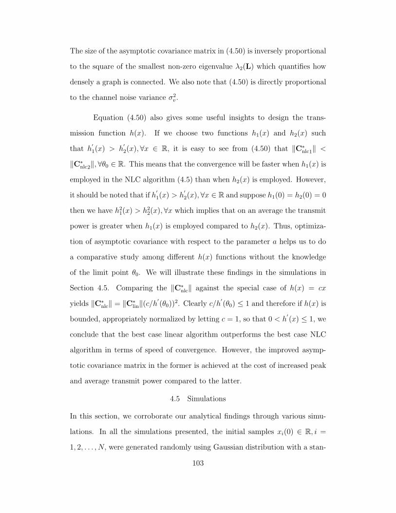
The size of the asymptotic covariance matrix in (4.50) is inversely proportional
to the square of the smallest non-zero eigenvalue λ2(L) which quantifies how
densely a graph is connected. We also note that (4.50) is directly proportional
to the channel noise variance σ2v .
Equation (4.50) also gives some useful insights to design the trans-
mission function h(x). If we choose two functions h1(x) and h2(x) such
that h′
1(x) > h′
2(x), ∀x ∈ R, it is easy to see from (4.50) that ‖C∗nlc1‖ <
‖C∗nlc2‖, ∀θ0 ∈ R. This means that the convergence will be faster when h1(x) is
employed in the NLC algorithm (4.5) than when h2(x) is employed. However,
it should be noted that if h′
1(x) > h′
2(x), ∀x ∈ R and suppose h1(0) = h2(0) = 0
then we have h21(x) > h2
2(x), ∀x which implies that on an average the transmit
power is greater when h1(x) is employed compared to h2(x). Thus, optimiza-
tion of asymptotic covariance with respect to the parameter a helps us to do
a comparative study among different h(x) functions without the knowledge
of the limit point θ0. We will illustrate these findings in the simulations in
Section 4.5. Comparing the ‖C∗nlc‖ against the special case of h(x) = cx
yields ‖C∗nlc‖ = ‖C∗
lin‖(c/h′
(θ0))2. Clearly c/h
′
(θ0) ≤ 1 and therefore if h(x) is
bounded, appropriately normalized by letting c = 1, so that 0 < h′
(x) ≤ 1, we
conclude that the best case linear algorithm outperforms the best case NLC
algorithm in terms of speed of convergence. However, the improved asymp-
totic covariance matrix in the former is achieved at the cost of increased peak
and average transmit power compared to the latter.
4.5 Simulations
In this section, we corroborate our analytical findings through various simu-
lations. In all the simulations presented, the initial samples xi(0) ∈ R, i =
1, 2, . . . , N, were generated randomly using Gaussian distribution with a stan-
103
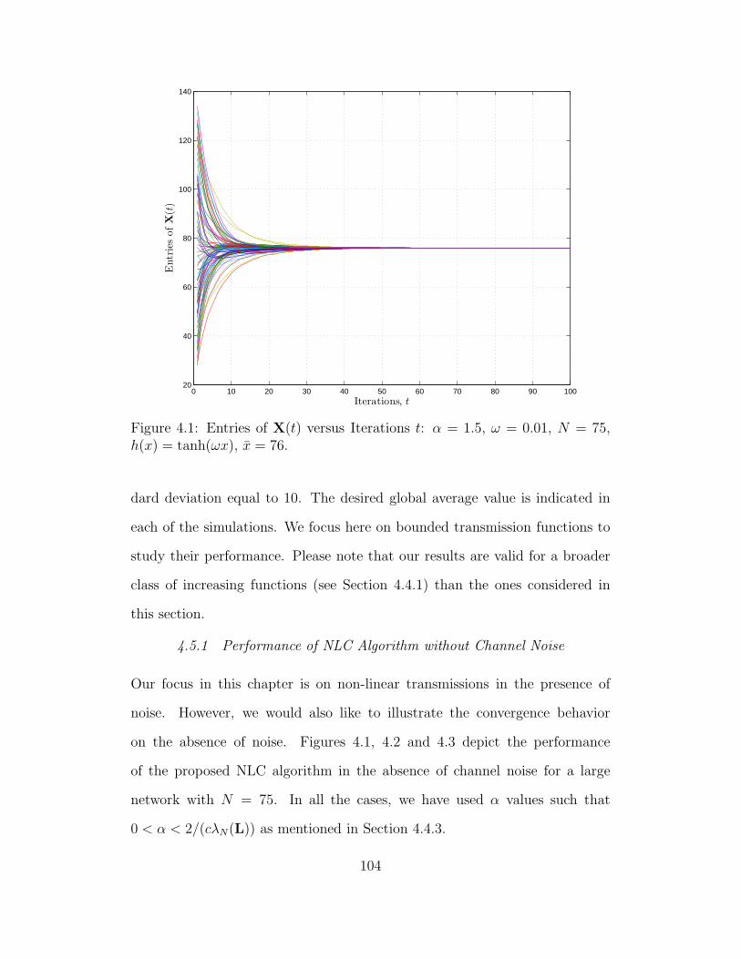
0 10 20 30 40 50 60 70 80 90 10020
40
60
80
100
120
140
Iterations, t
Entr
ies
ofX
(t)
Figure 4.1: Entries of X(t) versus Iterations t: α = 1.5, ω = 0.01, N = 75,h(x) = tanh(ωx), x = 76.
dard deviation equal to 10. The desired global average value is indicated in
each of the simulations. We focus here on bounded transmission functions to
study their performance. Please note that our results are valid for a broader
class of increasing functions (see Section 4.4.1) than the ones considered in
this section.
4.5.1 Performance of NLC Algorithm without Channel Noise
Our focus in this chapter is on non-linear transmissions in the presence of
noise. However, we would also like to illustrate the convergence behavior
on the absence of noise. Figures 4.1, 4.2 and 4.3 depict the performance
of the proposed NLC algorithm in the absence of channel noise for a large
network with N = 75. In all the cases, we have used α values such that
0 < α < 2/(cλN(L)) as mentioned in Section 4.4.3.
104
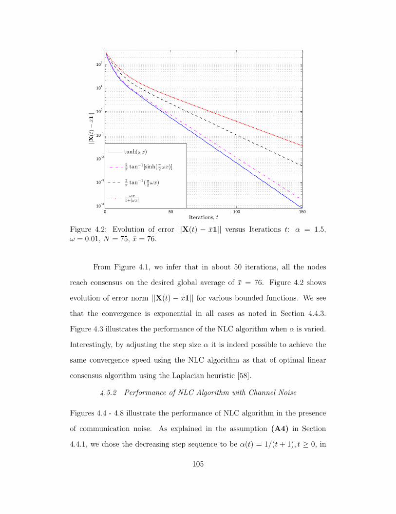
0 50 100 15010
−4
10−3
10−2
10−1
100
101
102
Iterations, t
||X(t
)−
x1||
tanh(ωx)
2
πtan−1[sinh(π
2ωx)]
2
πtan−1(π
2ωx)
ωx
1+|ωx|
Figure 4.2: Evolution of error ||X(t) − x1|| versus Iterations t: α = 1.5,ω = 0.01, N = 75, x = 76.
From Figure 4.1, we infer that in about 50 iterations, all the nodes
reach consensus on the desired global average of x = 76. Figure 4.2 shows
evolution of error norm ||X(t) − x1|| for various bounded functions. We see
that the convergence is exponential in all cases as noted in Section 4.4.3.
Figure 4.3 illustrates the performance of the NLC algorithm when α is varied.
Interestingly, by adjusting the step size α it is indeed possible to achieve the
same convergence speed using the NLC algorithm as that of optimal linear
consensus algorithm using the Laplacian heuristic [58].
4.5.2 Performance of NLC Algorithm with Channel Noise
Figures 4.4 - 4.8 illustrate the performance of NLC algorithm in the presence
of communication noise. As explained in the assumption (A4) in Section
4.4.1, we chose the decreasing step sequence to be α(t) = 1/(t + 1), t ≥ 0, in
105
0 10 20 30 40 50 60 7010
−8
10−6
10−4
10−2
100
102
Iterations, t
||X(t
)−
x1||
Non-Linear: α = 2
Non-Linear: α = 4
Non-Linear: α = 6
Non-Linear: α = 8
Linear Optimal: α∗ = 0.0283
Figure 4.3: Evolution of error ||X(t)− x1|| versus Iterations t: α = 2, 4, 6, 8,ω = 0.005, N = 75, h(x) = 2
πtan−1[sinh(π
2ωx)], x = 114.
all simulations. Here we assumed that ρ = maxx h2(x) is the maximum power
available at each sensor to transmit its state value. Figure 4.4 shows that the
nodes employing the NLC algorithm reach consensus for a small network with
N = 10. Figure 4.5 shows the transmit power h2(xi(t)), i = 1, 2, . . . , N, per-
neighbour versus iterations for a large network. Clearly, the transmit power
is always constrained within the upper bound of ρ (indicated by the dashed
line) making the proposed scheme practically viable for the power constrained
WSNs.
In Figures 4.6, 4.7 and 4.8, we show the convergence speed performance
of the proposed NLC algorithm by plotting ||E[X(t)]− x1|| versus iterations t.
These plots indicate how fast the mean of the process X(t) converges towards
the desired global mean vector x1.
106
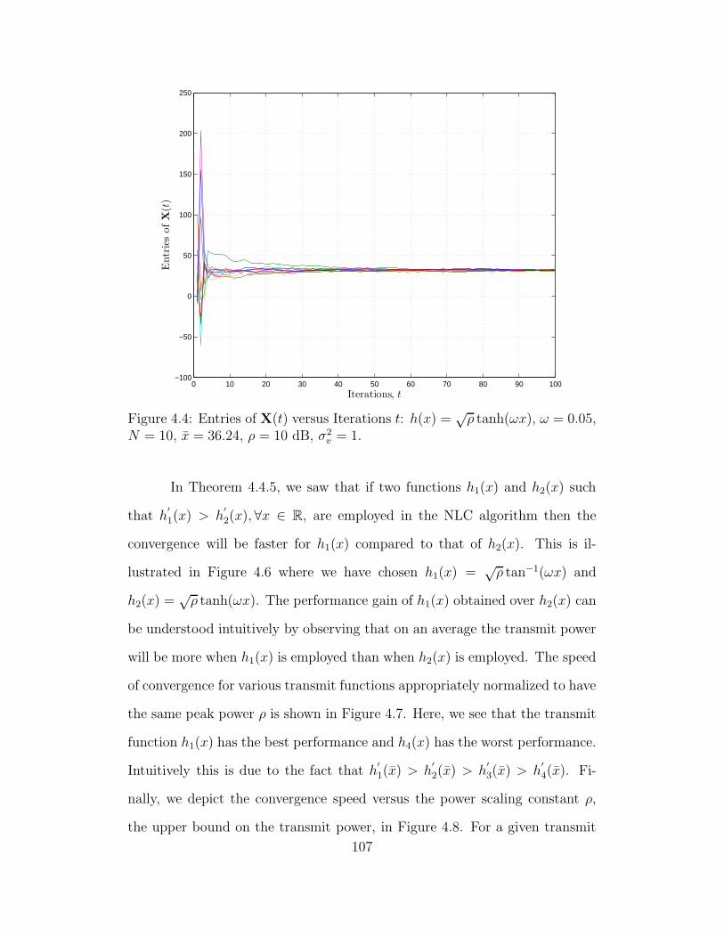
0 10 20 30 40 50 60 70 80 90 100−100
−50
0
50
100
150
200
250
Iterations, t
Entr
ies
ofX
(t)
Figure 4.4: Entries of X(t) versus Iterations t: h(x) =√ρ tanh(ωx), ω = 0.05,
N = 10, x = 36.24, ρ = 10 dB, σ2v = 1.
In Theorem 4.4.5, we saw that if two functions h1(x) and h2(x) such
that h′
1(x) > h′
2(x), ∀x ∈ R, are employed in the NLC algorithm then the
convergence will be faster for h1(x) compared to that of h2(x). This is il-
lustrated in Figure 4.6 where we have chosen h1(x) =√ρ tan−1(ωx) and
h2(x) =√ρ tanh(ωx). The performance gain of h1(x) obtained over h2(x) can
be understood intuitively by observing that on an average the transmit power
will be more when h1(x) is employed than when h2(x) is employed. The speed
of convergence for various transmit functions appropriately normalized to have
the same peak power ρ is shown in Figure 4.7. Here, we see that the transmit
function h1(x) has the best performance and h4(x) has the worst performance.
Intuitively this is due to the fact that h′
1(x) > h′
2(x) > h′
3(x) > h′
4(x). Fi-
nally, we depict the convergence speed versus the power scaling constant ρ,
the upper bound on the transmit power, in Figure 4.8. For a given transmit
107
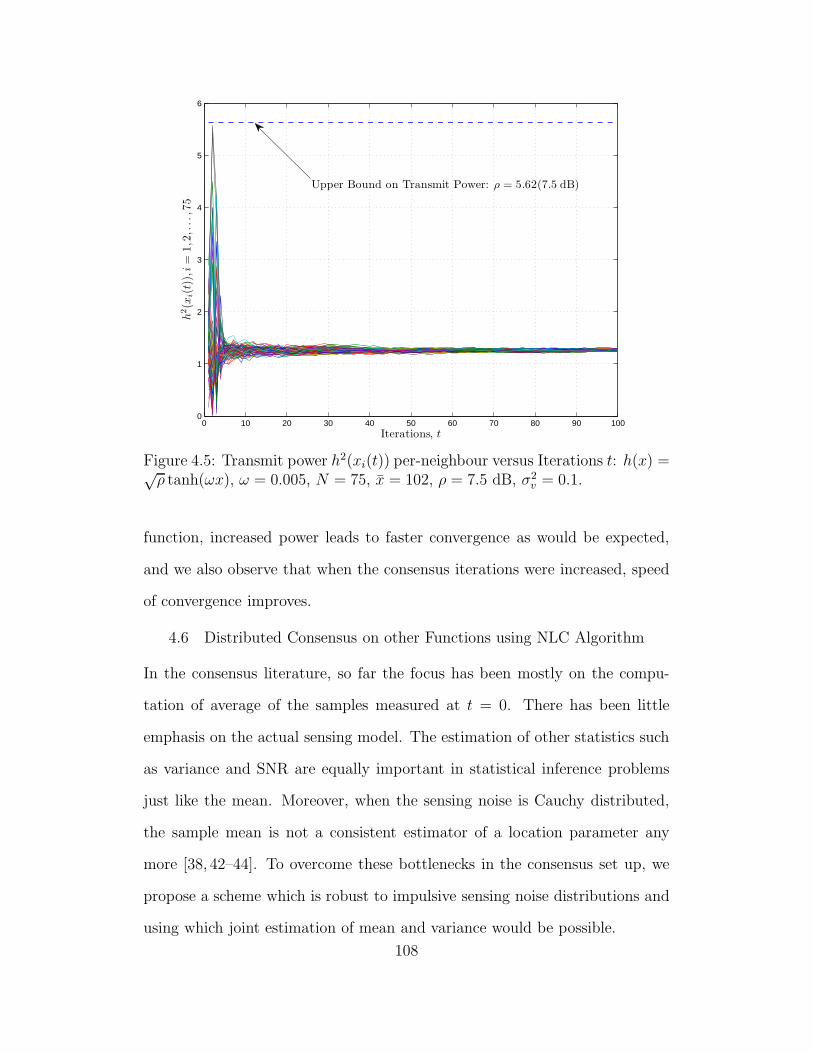
0 10 20 30 40 50 60 70 80 90 1000
1
2
3
4
5
6
Iterations, t
h2(x
i(t
)),i
=1,2
,...
,75
Upper Bound on Transmit Power: ρ = 5.62(7.5 dB)
Figure 4.5: Transmit power h2(xi(t)) per-neighbour versus Iterations t: h(x) =√ρ tanh(ωx), ω = 0.005, N = 75, x = 102, ρ = 7.5 dB, σ2
v = 0.1.
function, increased power leads to faster convergence as would be expected,
and we also observe that when the consensus iterations were increased, speed
of convergence improves.
4.6 Distributed Consensus on other Functions using NLC Algorithm
In the consensus literature, so far the focus has been mostly on the compu-
tation of average of the samples measured at t = 0. There has been little
emphasis on the actual sensing model. The estimation of other statistics such
as variance and SNR are equally important in statistical inference problems
just like the mean. Moreover, when the sensing noise is Cauchy distributed,
the sample mean is not a consistent estimator of a location parameter any
more [38, 42–44]. To overcome these bottlenecks in the consensus set up, we
propose a scheme which is robust to impulsive sensing noise distributions and
using which joint estimation of mean and variance would be possible.
108
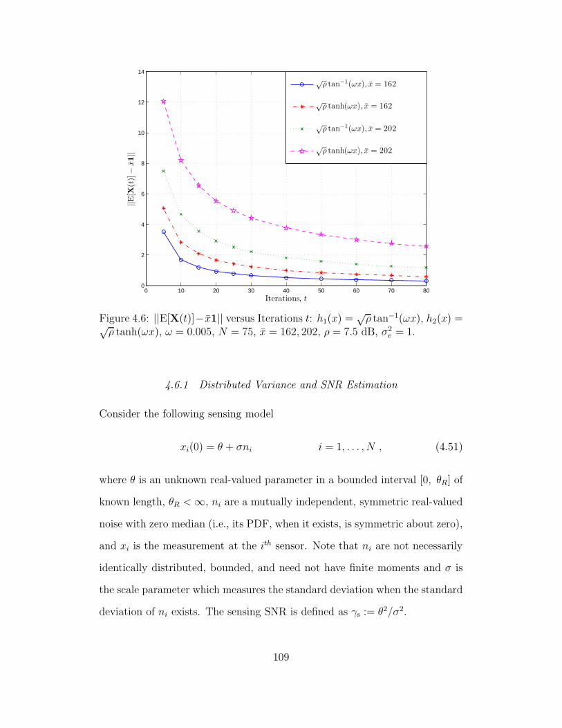
0 10 20 30 40 50 60 70 800
2
4
6
8
10
12
14
Iterations, t
||E[X
(t)]−
x1||
√
ρ tan−1(ωx), x = 162
√ρ tanh(ωx), x = 162
√ρ tan−1(ωx), x = 202
√ρ tanh(ωx), x = 202
Figure 4.6: ||E[X(t)]−x1|| versus Iterations t: h1(x) =√ρ tan−1(ωx), h2(x) =√
ρ tanh(ωx), ω = 0.005, N = 75, x = 162, 202, ρ = 7.5 dB, σ2v = 1.
4.6.1 Distributed Variance and SNR Estimation
Consider the following sensing model
xi(0) = θ + σni i = 1, . . . , N , (4.51)
where θ is an unknown real-valued parameter in a bounded interval [0, θR] of
known length, θR < ∞, ni are a mutually independent, symmetric real-valued
noise with zero median (i.e., its PDF, when it exists, is symmetric about zero),
and xi is the measurement at the ith sensor. Note that ni are not necessarily
identically distributed, bounded, and need not have finite moments and σ is
the scale parameter which measures the standard deviation when the standard
deviation of ni exists. The sensing SNR is defined as γs := θ2/σ2.
109
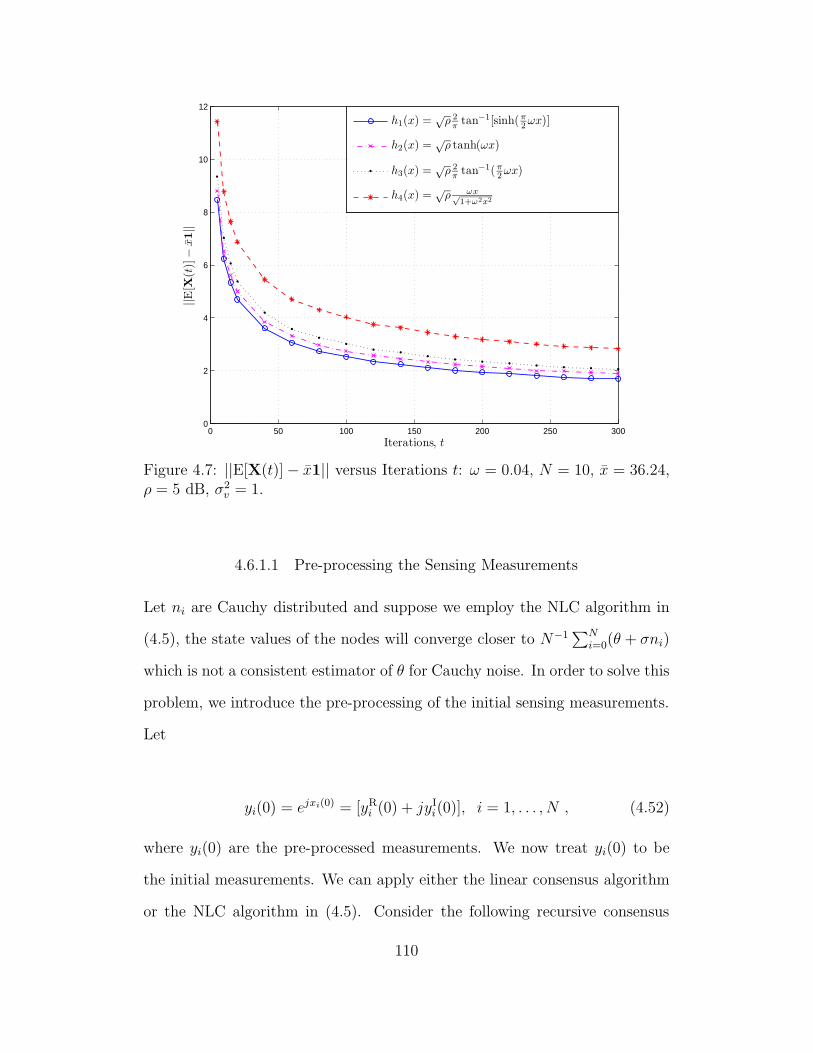
0 50 100 150 200 250 3000
2
4
6
8
10
12
Iterations, t
||E[X
(t)]−
x1||
h1(x) =√
ρ 2
πtan−1[sinh(π
2ωx)]
h2(x) =√
ρ tanh(ωx)
h3(x) =√
ρ 2
πtan−1(π
2ωx)
h4(x) =√
ρ ωx√1+ω2x2
Figure 4.7: ||E[X(t)]− x1|| versus Iterations t: ω = 0.04, N = 10, x = 36.24,ρ = 5 dB, σ2
v = 1.
4.6.1.1 Pre-processing the Sensing Measurements
Let ni are Cauchy distributed and suppose we employ the NLC algorithm in
(4.5), the state values of the nodes will converge closer to N−1∑N
i=0(θ + σni)
which is not a consistent estimator of θ for Cauchy noise. In order to solve this
problem, we introduce the pre-processing of the initial sensing measurements.
Let
yi(0) = ejxi(0) = [yRi (0) + jyIi(0)], i = 1, . . . , N , (4.52)
where yi(0) are the pre-processed measurements. We now treat yi(0) to be
the initial measurements. We can apply either the linear consensus algorithm
or the NLC algorithm in (4.5). Consider the following recursive consensus
110
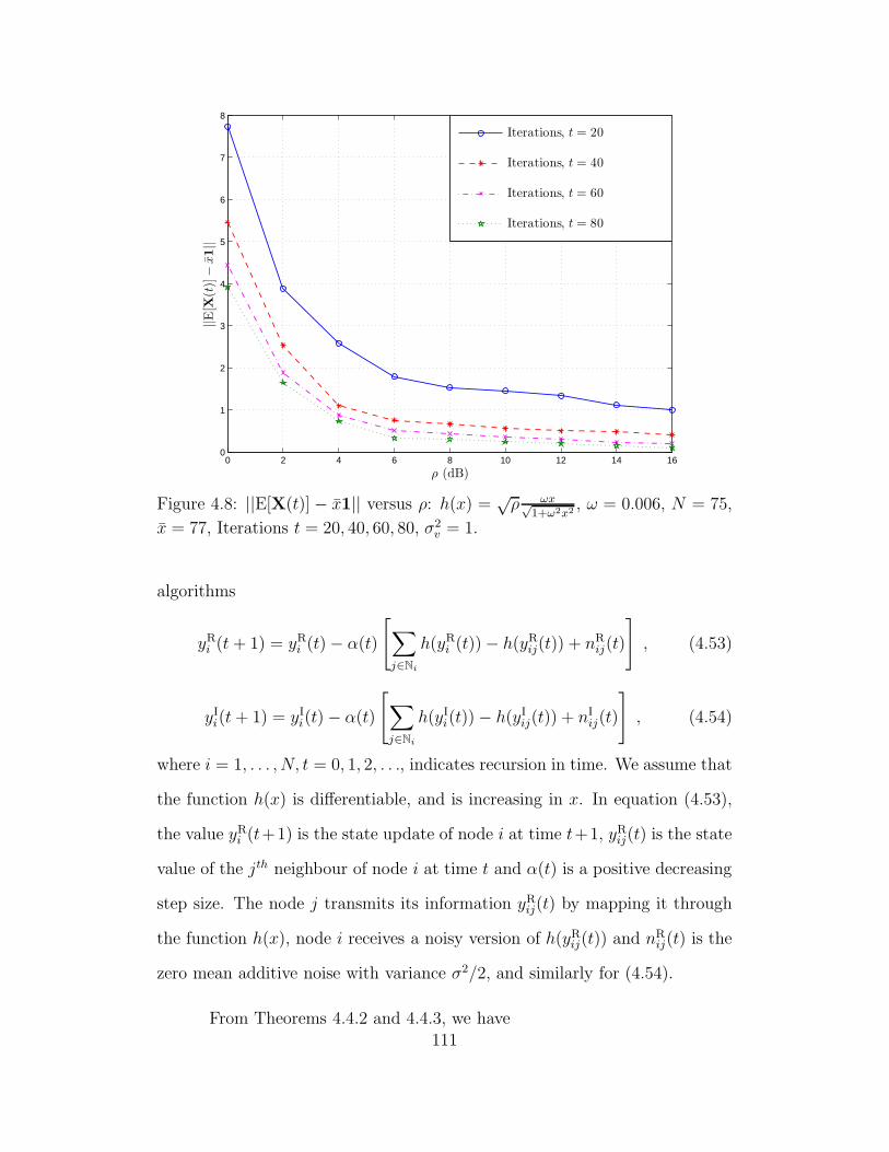
0 2 4 6 8 10 12 14 160
1
2
3
4
5
6
7
8
ρ (dB)
||E[X
(t)]−
x1||
Iterations, t = 20
Iterations, t = 40
Iterations, t = 60
Iterations, t = 80
Figure 4.8: ||E[X(t)]− x1|| versus ρ: h(x) = √ρ ωx√
1+ω2x2, ω = 0.006, N = 75,
x = 77, Iterations t = 20, 40, 60, 80, σ2v = 1.
algorithms
yRi (t + 1) = yRi (t)− α(t)
[∑
j∈Ni
h(yRi (t))− h(yRij(t)) + nRij(t)
], (4.53)
yIi(t+ 1) = yIi(t)− α(t)
[∑
j∈Ni
h(yIi(t))− h(yIij(t)) + nIij(t)
], (4.54)
where i = 1, . . . , N, t = 0, 1, 2, . . ., indicates recursion in time. We assume that
the function h(x) is differentiable, and is increasing in x. In equation (4.53),
the value yRi (t+1) is the state update of node i at time t+1, yRij(t) is the state
value of the jth neighbour of node i at time t and α(t) is a positive decreasing
step size. The node j transmits its information yRij(t) by mapping it through
the function h(x), node i receives a noisy version of h(yRij(t)) and nRij(t) is the
zero mean additive noise with variance σ2/2, and similarly for (4.54).
From Theorems 4.4.2 and 4.4.3, we have111
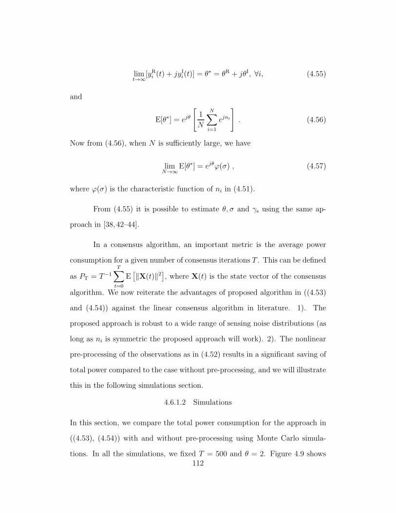
limt→∞
[yRi (t) + jyIi(t)] = θ∗ = θR + jθI, ∀i, (4.55)
and
E[θ∗] = ejθ
[1
N
N∑
i=1
ejni
]. (4.56)
Now from (4.56), when N is sufficiently large, we have
limN→∞
E[θ∗] = ejθϕ(σ) , (4.57)
where ϕ(σ) is the characteristic function of ni in (4.51).
From (4.55) it is possible to estimate θ, σ and γs using the same ap-
proach in [38, 42–44].
In a consensus algorithm, an important metric is the average power
consumption for a given number of consensus iterations T . This can be defined
as PT = T−1
T∑
t=0
E[‖X(t)‖2
], where X(t) is the state vector of the consensus
algorithm. We now reiterate the advantages of proposed algorithm in ((4.53)
and (4.54)) against the linear consensus algorithm in literature. 1). The
proposed approach is robust to a wide range of sensing noise distributions (as
long as ni is symmetric the proposed approach will work). 2). The nonlinear
pre-processing of the observations as in (4.52) results in a significant saving of
total power compared to the case without pre-processing, and we will illustrate
this in the following simulations section.
4.6.1.2 Simulations
In this section, we compare the total power consumption for the approach in
((4.53), (4.54)) with and without pre-processing using Monte Carlo simula-
tions. In all the simulations, we fixed T = 500 and θ = 2. Figure 4.9 shows112
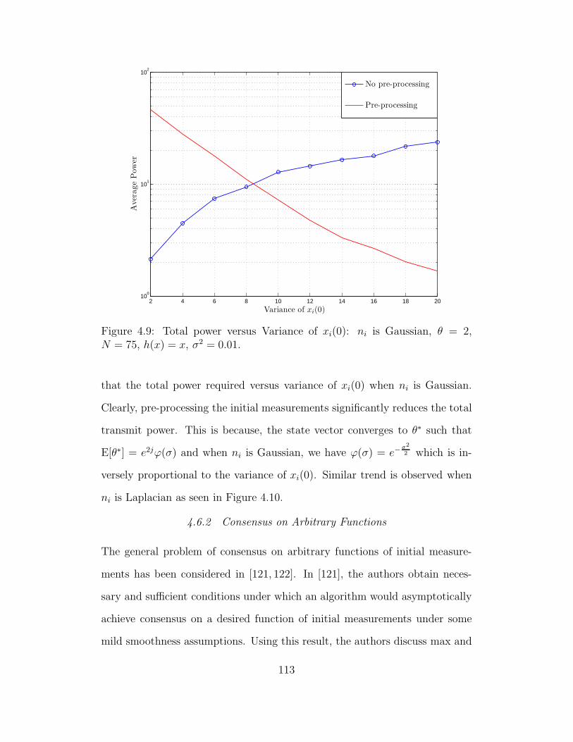
2 4 6 8 10 12 14 16 18 2010
0
101
102
Variance of xi(0)
Aver
age
Pow
er
No pre-processing
Pre-processing
Figure 4.9: Total power versus Variance of xi(0): ni is Gaussian, θ = 2,N = 75, h(x) = x, σ2 = 0.01.
that the total power required versus variance of xi(0) when ni is Gaussian.
Clearly, pre-processing the initial measurements significantly reduces the total
transmit power. This is because, the state vector converges to θ∗ such that
E[θ∗] = e2jϕ(σ) and when ni is Gaussian, we have ϕ(σ) = e−σ2
2 which is in-
versely proportional to the variance of xi(0). Similar trend is observed when
ni is Laplacian as seen in Figure 4.10.
4.6.2 Consensus on Arbitrary Functions
The general problem of consensus on arbitrary functions of initial measure-
ments has been considered in [121, 122]. In [121], the authors obtain neces-
sary and sufficient conditions under which an algorithm would asymptotically
achieve consensus on a desired function of initial measurements under some
mild smoothness assumptions. Using this result, the authors discuss max and
113
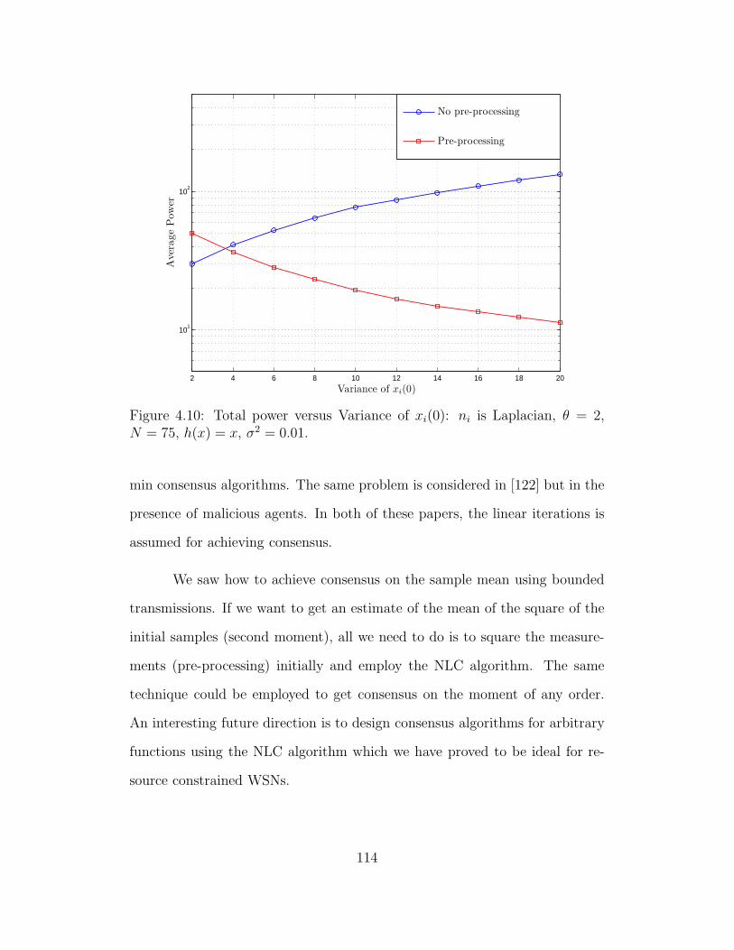
2 4 6 8 10 12 14 16 18 20
101
102
Variance of xi(0)
Aver
age
Pow
er
No pre-processing
Pre-processing
Figure 4.10: Total power versus Variance of xi(0): ni is Laplacian, θ = 2,N = 75, h(x) = x, σ2 = 0.01.
min consensus algorithms. The same problem is considered in [122] but in the
presence of malicious agents. In both of these papers, the linear iterations is
assumed for achieving consensus.
We saw how to achieve consensus on the sample mean using bounded
transmissions. If we want to get an estimate of the mean of the square of the
initial samples (second moment), all we need to do is to square the measure-
ments (pre-processing) initially and employ the NLC algorithm. The same
technique could be employed to get consensus on the moment of any order.
An interesting future direction is to design consensus algorithms for arbitrary
functions using the NLC algorithm which we have proved to be ideal for re-
source constrained WSNs.
114
Chapter 5
Robust Consensus with Receiver Non-Linearity
5.1 Literature Survey and Motivation
In Chapter 4, we saw that the non-linear mapping was done at the transmit
node before transmitting the state information and we proved convergence
and convergence rate results. In existing literature on consensus (please see
[63, 65, 67, 123–129] and references therein) which discuss consensus in the
presence of communication noise, the additive noise is assumed to have finite
moments. All the existing consensus algorithms will fail if the communication
noise does not have finite second moment such as in the case of Cauchy noise.
Sensor networks which operate in adverse conditions require algorithms which
are robust to impulsive channel noise distributions. Therefore there is a need
to develop consensus algorithms which are impervious to impulsive channel
noise (like Cauchy) by performing some nonlinear operation at the receiver
node. Moreover, consensus with nonlinear combining at the receiver has been
considered in [60,113] only in the absence of inter-sensor communication noise.
Therefore, it is of interest to solve the problem of distributed consensus with
receiver non-linearity when there is communication noise.
In this chapter, we propose a robust nonlinear distributed consensus
(RNLC) algorithm which is robust to impulsive communication noise by per-
forming nonlinear processing at the receiver sensor node. We consider a more
general class of channel noise distributions than the very restricted class of
noise distributions considered in the literature. We do not require the chan-
nel noise to have finite moments as is assumed in all the previous work on
distributed average consensus algorithms, please see [63, 65, 67, 123–129]. We
only need the channel noise to be a zero median symmetric random variable,
115
i.e., the probability density function (PDF) is symmetric about zero. In addi-
tion, we also assume that every sensor maps its state value through a bounded
function before transmission so that the transmit power at every node in every
iteration is always bounded, making it ideal for resource-constrained WSNs.
The analysis of the RNLC algorithm with both the transmit and receiver non-
linearities in the presence of channel noise is non-trivial. We prove that all
the sensors employing the RNLC algorithm reach consensus to a finite ran-
dom variable whose mean is the desired sample average. We characterize the
asymptotic performance by deriving the asymptotic covariance matrix using
results from stochastic approximation theory. Finally we explore the perfor-
mance of the proposed algorithm employing various functions for the transmit
and receiver non-linearities. Different from [63, 65, 67] which also considered
consensus in the presence of noisy transmissions, herein we analyse nonlinear
processing both at the transmit and receiver nodes and study the asymptotic
covariance matrix and its dependence on both the non-linearities. Our work
in this chapter also shows an interesting relationship between the Fisher in-
formation and the asymptotic covariance matrix which comes out as a result
of having nonlinear processing at the receiver sensor node. To the best of
our knowledge, we are the first ones in the consensus literature to propose a
consensus algorithm which relaxes the requirement of finite moments on the
communication noise.
The rest of this chapter is organized as follows. In Section 5.2, we
describe the system model and review the previous work on non-linear con-
sensus. We consider the RNLC algorithm in the presence of noise in Section
5.3, and prove that the sensors reach consensus to a random variable. In Sec-
116

tion 5.4, we present several simulation examples to study the performance of
the proposed algorithm.
We will use the same notations used in the previous chapter. We note
that we will drop the index of some variables for convenience and the intention
will be clear from the context.
5.2 System Model and Previous Work5.2.1 System Model
Consider a WSN withN sensor nodes each with an initial measurement xi(0) ∈
R. Measurements made at the sensor nodes are modeled as
xi(0) = θ + ni , i = 1, . . . , N (5.1)
where θ is an unknown real-valued parameter and ni is the sensing noise at
the ith sensor. The sample mean of these initial measurements in (5.1) is given
by
x =1
N
N∑
i=1
xi(0) . (5.2)
Let x be the estimate of the parameter θ to be computed by an iterative
distributed algorithm, in which each sensor communicates only with its neigh-
bours. If the states of all the sensor nodes converge to x, then the network is
said to have reached consensus on the sample average.
5.2.2 Previous Work
A commonly used iterative algorithm for distributed consensus can be written
as
xi(t+ 1) = xi(t)− α∑
j∈Ni
h(xi(t)− xij(t)) , (5.3)
where i = 1, . . . , N , t = 0, 1, 2, . . ., is the time index, xi(t + 1) is the updated
state value of sensor node i at time t+ 1, Ni is the set of neighbours of sensor117
node i, xij(t), j ∈ Ni are the state values of the neighbours of sensor node i at
time t, and α is a constant step size. If h(·) is linear, then (5.3) is a linear dis-
tributed average-consensus (LDAC) algorithm [58,61,62]. In [58], it is proved
that if 0 < α < 2/λN(L), then xi(t) converges to x exponentially and (5.3) is
then called as the LDAC algorithm based on the Laplacian heuristic. If h(·)
is non-linear then the algorithm belongs to the class of non-linear distributed
average-consensus algorithms [60,113]. In [60], the average consensus problem
is solved when h(x) in (5.3) is differentiable and odd. In [113], it is illustrated
that when h(x) in (5.3) is sin(x), faster convergence is possible compared to
the LDAC algorithm based on the Laplacian heuristic. In all of these cases,
xij(t) has to be transmitted to node i before it can apply the function h(·) to
get the new updated state value. Therefore, the transmit peak power in (5.3)
is determined by xi(t) and not necessarily bounded, even if h(·) is bounded.
Moreover, there is no communication noise assumed in all the previous work
on non-linear consensus.
5.3 Robust Consensus with Impulsive Communication Noise
In this work, we propose a robust distributed nonlinear average consensus
algorithm in which every node also performs a nonlinear operation upon the
receiving the state values from its neighbours. Every sensor also maps its state
value through a bounded function before transmission to constrain the trans-
mit power. Therefore the magnitude of the transmitted signal at every node
in every iteration is always bounded making it ideal for resource-constrained
WSNs and the receiver non-linearity makes the algorithm robust to a wide
range of channel noise distributions.
In this section, we will study the RNLC algorithm with communica-
tion noise when sensors exchange information. Our approach is similar to,
118
but more general than [65] and [98] in that we analyse non-linearity at both
the receiver and transmit sensor nodes. Moreover, unlike [65] we study the
asymptotic covariance matrix of the state vector and its dependence on the
non-linearity. Unlike [113] and [60], we assume receiver non-linearity in the
presence of communication noise which brings us the benefit of robustness to
a wide range of noise distributions.
5.3.1 The RNLC Algorithm with Communication Noise
Let each sensor map its state value at time t through the function h(x) be-
fore transmission, and combines the received state values through a nonlinear
function according to the following RNLC algorithm:
xi(t+ 1) = xi(t)− α(t)∑
j∈Ni
[f (h(xi(t))− h(xij(t)) + nij(t))] , (5.4)
where i = 1, . . . , N, t = 0, 1, 2, . . ., is the time index. The value xi(t + 1) is
the state update of node i at time t + 1, xij(t) is the state value of the jth
neighbour of node i at time t and α(t) is a positive step size which will further
be assumed to satisfy assumption (A5) in the sequel. The node j transmits
its information xij(t) by mapping it through the function h(x), node i receives
a noisy version of h(xij(t)) and nij(t) is the noise associated with the reception
of h(xij(t)). The function f(x) is applied at the receiver side to combat the
effect of impulsive channel noise and will be further assumed to satisfy (A2)
in the sequel.
Note that the proposed scheme (5.4) is different from (5.3) in the fol-
lowing aspects. Firstly, in (5.3), xij(t) has to be transmitted which could
exhibit variation over a wide range of values if xi(0) has a large dynamic range
and hence (5.3) does not guarantee bounded transmission power. In contrast,
in the proposed scheme the non-linearity is applied before the state value is
119
transmitted so that the magnitude of the transmitted state value is always
constrained within the maximum value of h(x) irrespective of the range of
xi(t) and the realizations of noise nij(t). Finally, (5.4) involves communica-
tion noise while (5.3) does not. Thus the proposed scheme is more suited
to resource constrained WSNs when compared to (5.3), and it is practically
viable for WSNs operating in adverse conditions.
Our model in (5.4) is more general than the linear consensus algorithm
considered in [65] which is a special case when f(x) and h(x) are linear. We
make the following assumptions on f(x), h(x), nij(t), α(t) and the graph:
Assumptions
(A1): The graph G is connected so that λ2(L) > 0.
(A2): The function f(x) is strictly increasing, odd such that for a given x,
the variance var[f(x + n)] ≤ σ2 is bounded (we have dropped the indices of
the noise samples nij(t) for convenience).
(A3): The function h(x) is differentiable, and has a bounded derivative
such that 0 < h′
(x) ≤ c, for some c > 0.
(A4) Independent Noise Sequence: The noise samples nij(t) are mu-
tually independent identically distributed (i.i.d.), symmetric real-valued with
zero median (i.e., its PDF symmetric about zero). Note that nij(t) are not
necessarily bounded, and need not have finite moments. We make no distri-
butional assumptions on the communication noise PDF. Note that this as-
sumption is more general than [63, 65, 67, 123–129] in that they require the
communication noise to have finite moments whereas we do not require finite
mean or variance for the noise distribution.
(A5) Decreasing Weight Sequence: Even though var[f(x+n)] is bounded,
the recursive nature of (5.6) could make the algorithm diverge. In order to
120
control the variance growth rate of the noise we need the following conditions
on the sequence α(t):
α(t) > 0 ,∞∑
t=0
α(t) = ∞ ,∞∑
t=0
α2(t) < ∞ . (5.5)
Let g(x) := En [f(x+ n)] where E(·) denotes the expectation so that
f(x+ n) = g(x) + n(x). It can be easily proved that g(x) is an odd function
under the assumptions (A2), (A3) and (A4), and hence g(0) = 0. Clearly
E[n(x)] = 0 and E[n2(x)] ≤ σ2. Using g(x) the recursion in (5.4) can be
written in vector form as
X(t+ 1) = X(t)− α(t) [µ(X(t)) + n(t,X(t))] . (5.6)
where X(t) is state vector at time t given by X(t) = [x1(t) x2(t) . . . xN(t)]T,
and µ : RN → RN such that its ith element is given by
µi(X(t)) =∑
j∈Ni
g(h(xi(t))− h(xij(t))) , 1 ≤ i ≤ N . (5.7)
The vector n(t,X(t)) captures the additive noise at N nodes contributed by
their respective neighbours and their state values and its ith component is
given by
ni(t,X(t)) = −∑
j∈Ni
n(t, xi(t), xij(t)) , 1 ≤ i ≤ N . (5.8)
Clearly, conditioned on X(t), the channel noise {n(t, xi(t), xij(t))}t≥0,1≤i,j≤N
is an independent sequence across time and space. It also satisfies
E[n(t,X(t))] = 0 , ∀t , µ := supt
E[‖n(t,X(t))‖2] ≤ Ndmaxσ2 < ∞. (5.9)
Note that (5.9) is because of the fact that the number of neighbours of a given
node is upper bounded by dmax.
Our primary motivation for considering non-linear processing is two
fold: 1). We want to develop a consensus algorithm that is robust to the121
impulsive communication noise which do not necessarily have finite moments.
We accomplish this by the receiver nonlinear function f(·) as it will be shown
in Theorem 5.3.1; 2). We want to impose the realistic assumption of bounded
peak per-sensor power by ensuring that the transmit nonlinear function h(·)
is bounded.
We will prove convergence and asymptotic normality result of the RNLC
algorithm in (5.6) using the same approach used in Chapter 4. Recall the re-
sult on the convergence of a discrete time Markov process which will now be
used in establishing convergence of the RNLC algorithm in (5.6).
To prove the a.s. convergence of the consensus algorithm in (5.6) using
Theorem 4.4.1, we define the consensus subspace B, the set of all vectors whose
entries are of equal value as,
B = {x ∈ RN |x = a1 , a ∈ R} . (5.10)
We are now ready to state the main result of Section 5.3.
Theorem 5.3.1. Let the assumptions (A1), (A2), (A4) and (A5) hold,
and assume h(x) is strictly increasing. Consider the RNLC algorithm in (5.6)
with the initial state vector X(0) ∈ RN . Then, the state vector X(t) in (5.6)
approaches the consensus subspace B a.s., i.e.,
Pr
[limt→∞
infY∈B
‖X(t)−Y‖ = 0
]= 1. (5.11)
Proof. We will make use of Theorem 4.4.1 to prove (5.11). We will choose
an appropriate potential function V (x) that is non-negative which satisfies
equation (4.11). We will then prove that the generating operator L applied
122
on V (x) as in (4.10) can be upper bounded as in (4.12) with γ(t) = α(t), and
a ϕ(x) can be found that satisfies (4.13).
First we see that under the assumptions (A1), (A2), (A4) and the
assumption on h(x), the discrete time vector process {X(t)}t≥0 is Markov.
Define a positive semi-definite matrix M such that mij = −1, i 6= j, mii =
N − 1. Let V (x) = xTMx, then the function V (x) is non-negative since M
is a positive semi-definite matrix by construction. Note that x ∈ B is an
eigenvector of M associated with the zero eigenvalue, therefore we have
V (x) = 0,x ∈ B . (5.12)
Let x = xB + xB⊥ where xB is the orthogonal projection of x on B. When
x ∈ B′
, we have ‖xB⊥‖ > 0. Let x ∈ B′
and µ(x) be as defined in (5.6). Then,
µ(x) = µB(x) + µB⊥(x), where µB⊥(x) is non-zero, i.e., ‖µB⊥(x)‖ > 0 which
is proved now. First we note that xTMµ(x) > 0 (please see equations (5.23)
through (5.29). This means (xB+xB⊥)M(µB(x)+µB⊥(x)) = xB⊥MµB⊥(x) >
0. If µB⊥(x) were zero, then xB⊥MµB⊥(x) = 0 which contradicts with the
fact that xB⊥MµB⊥(x) > 0. Therefore, µB⊥(x) is non-zero. Define β :=
‖µB⊥(x)‖2/‖xB⊥‖2, then β > 0, x ∈ B′
. Therefore, for any x ∈ B′
,
V (x) = xTMx = V (xB + xB⊥) = V (xB⊥)
≥ minxB⊥ 6=0
xTB⊥MxB⊥ = λ2(M)‖xB⊥‖2 > 0 , (5.13)
where the last inequality is due to λ2(L) > 0 by assumption (A1). The
equations (5.12) and (5.13) establish that the conditions in (4.11) in Theorem
4.4.1 are satisfied.
123
Now we will prove that (4.12) is satisfied as well. Towards this end,
consider LV (x) defined in (4.10),
LV (x) = E[X(t+ 1)TMX(t+ 1)|X(t) = x
]− V (x) , (5.14)
= E[(xT − α(t)
(µ(x)T + nT(t,x)
))·
(Mx− α(t) (Mµ(x) +Mn(t,x)))]− V (x) , (5.15)
= −2α(t)[xTMµ(x)
]+ α2(t)
[µ(x)TMµ(x) + E
[nT(t,x)Mn(t,x)
]].
(5.16)
We get (5.16) by expanding (5.15) and taking the expectations and using the
fact that E[n(t)] = 0. We have
E[nT(t,x)Mn(t,x)
]≤ E
[λN(M)‖nT(t,x)‖2
]≤ λN(M)µ, (5.17)
where the second inequality follows from (5.9). Using (5.17) in (5.16), we get
the following bound
LV (x) ≤ −2α(t)[xTMµ(x)
]+ α2(t)
[µ(x)TMµ(x) + µλN(M)
], (5.18)
≤ −2α(t)[xTMµ(x)
]+ α2(t)
[λN(M)β‖xB⊥‖2 + µλN(M)
], (5.19)
≤ −2α(t)[xTMµ(x)
]+ α2(t)
[βλN (M)
λ2(M)xTMx + µλN(M)
], (5.20)
≤ −2α(t)[xTMµ(x)
]+mα2(t)
[1 + β2x
TMx], (5.21)
≤ −α(t)ϕ(x) +mα2(t) [1 + V (x)] , (5.22)
where ϕ(x) := 2xTMµ(x), m := max{βλN(M)/λ2(M), λN(M)µ}, β2 :=
µλN(M)/m and β2 ∈ (0, 1]. In (5.19), we have used the fact µ(x)TMµ(x) ≤
λN(M)‖µB⊥(x)‖2 and ‖µB⊥(x)‖2 = β‖xB⊥‖2. In (5.20), we have used the fact
that xTMx ≥ λ2(M)‖xB⊥‖2 due to (5.13). We will now prove that ϕ(x) in
(5.22) satisfies equation (4.13) of Theorem 4.4.1.
124
Whenever x ∈ B, i.e., x = a1, a ∈ R, then xi = xj , ∀i, j, which means
g(h(xi) − h(xj)) = 0, ∀i, j, and hence µ(x) = 0. This implies that ϕ(x) =
0, ∀x ∈ B.
To prove ϕ(x) > 0 when x ∈ B′
, consider ϕ(x) = 2xTMµ(x) with M
of dimension N ×N ,
ϕ(x) = 2
[x1 x2 x3 . . . xN
]
N − 1 −1 −1 . . . −1
−1 N − 1 −1 . . . −1
−1 −1 N − 1 . . . −1
......
... . . ....
−1 −1 −1 . . . N − 1
µ(x)
(5.23)
= 2
N−1∑
k=1
xTµ(x)− 2
{[x2 x3 x4 . . . xN x1
]+
[x3 x4 x5 . . . x1 x2
]+
. . .[xN x1 x2 . . . xN−2 xN−1
]+
[x1 x2 x3 . . . xN−1 xN
]−
[x1 x2 x3 . . . xN−1 xN
] }µ(x) (5.24)
= 2[(N − 1)xT
µ(x)−[N(x1 + x2 + . . .+ xN)1
Tµ(x)
]+ xT
µ(x)]
(5.25)
= 2NxTµ(x) , (5.26)
where we get (5.25) by expanding the terms in the curly braces in (5.24) and
simplifying and we have used the fact that 1Tµ(x) = 0 in (5.25) to get (5.26).
125
Now consider
ϕ(x) = 2NxTµ(x) (5.27)
= 2N
[∑
j∈N1
g(h(x1)− h(xj))x1 +∑
j∈N2
g(h(x2)− h(xj))x2
+ . . .+∑
j∈NN
g(h(xN)− h(xj))xN
], (5.28)
where (5.28) follows from the symmetric structure of the graph. Note that
the ith summation in (5.28) corresponds to the ith node. Now suppose that
node i is connected to node j. Then there exists a term g(h(xi)− h(xj))xi in
the summation corresponding to the ith node in (5.28), and a term g(h(xj)−
h(xi))xj in the summation corresponding to the jth node in (5.28). Both of
these terms can be combined as (xi−xj)g(h(xi)−h(xj)) and this corresponds to
the edge {i, j} ∈ E. Thus equation (5.28) can be written as pairwise products
enumerated over all the edges in the graph as follows
ϕ(x) = 2N∑
{i,j}∈E(xi − xj) g(h(xi)− h(xj)) . (5.29)
Since x ∈ B′
, ϕ(x) in (5.29) is positive due to the facts that h(x) is strictly
increasing and g(x) is strictly an increasing odd function so that there is
at least one term in the sum which is strictly greater than zero. Letting
γ(t) = α(t), g(t) = α2(t) and by assumption (A5), we see that the sequence
α(t) in (5.22) satisfies (4.14). Thus all the conditions of Theorem 4.4.1 are
satisfied to yield (5.11).
Theorem 5.3.1 states that the sample paths of X(t) approach the con-
sensus subspace almost surely. We note that the assumption (A3) is not
necessary for Theorem 5.3.1 to hold. Instead we assumed h(x) is strictly in-
creasing (not necessarily differentiable) to prove Theorem 5.3.1. Now, like126
in [65], we will prove the convergence of X(t) to a finite point in B in Theorem
5.3.2.
Theorem 5.3.2. Let the assumptions of Theorem 5.3.1 hold. Consider the
RNLC algorithm in (5.6) with the initial state X(0) ∈ RN . Then, there exists
a finite real random variable θ∗ such that
Pr[limt→∞
X(t) = θ∗1]= 1. (5.30)
Proof. Let the average ofX(t) be x(t) = 1TX(t)/N . Since 1x(t) ∈ B, Theorem
5.3.1 implies,
Pr[limt→∞
‖X(t)− x(t)1‖ = 0]= 1 , (5.31)
where (5.31) follows from (5.11) since the infimum in (5.11) is achieved by
Y = x(t)1. Pre-multiplying (5.6) by 1T/N on both sides and noting that
1Tµ(x) = 0 due to the symmetric structure of the graph we get,
x(t+ 1) = x(t)− v(t) (5.32)
= x(0)−∑
0≤k≤t
v(k) (5.33)
where v(t) = α(t)1Tn(t,X(t))/N . From (5.9) it follows that
E[v(t)] = 0,
∑
t≥0
E[v(t)]2 =∑
t≥0
α2(t)
N2E‖n(t,X(t))‖2 ≤ µ
N2
∑
t≥0
α2(t) < ∞
which implies
E[x(t + 1)]2 ≤ x2(0) +µ
N2
∑
t≥0
α2(t) , ∀t . (5.34)
127
Equation (5.34) implies that the sequence {x(t)}t≥0 is an L2 bounded mar-
tingale 1 and hence converges a.s. and in L2 to a finite random variable θ∗
(see [118, Theorem 2.6.1]). Therefore the theorem follows from (5.31).
It should be noted that the results in Theorems 5.3.1 and 5.3.2 are
similar to the results in [65], but we have proved it for a more general case of
which [65] is a special case when f(x) = x and h(x) = x, and [98] is a special
case of (5.6) when f(x) = x. In what follows, we present the properties of the
limiting random variable θ∗.
5.3.2 Mean Square Error of RNLC Algorithm
The Theorems 5.3.1 and 5.3.2 establish that the sensors reach consensus
asymptotically and converge a.s. to a finite random variable θ∗. We can
view θ∗ as an estimate of x. In the following theorem we characterize the
unbiasedness and means squared error (MSE) properties of θ∗. We define the
MSE of θ∗ as ξN= E[(θ∗ − x)2].
Theorem 5.3.3. Let θ∗ be the limiting random variable as in Theorem 5.3.2.
Then θ∗ is unbiased, E[θ∗] = x, and its MSE is bounded, ξN≤ µN−2
∑
t≥0
α2(t).
The proof is obtained by following the same steps of the Lemma 5
in [65].
We point out that with non-linear processing, we have obtained a simi-
lar bound on the MSE ξNas that of the linear consensus algorithm in [65] but in
our case the bound depends on the functions f(x) and h(x). It should be noted
that µ ≤ Ndmaxσ2 from (5.9) which implies that ξ
N≤ dmaxN
−1∑
t≥0 α2(t)σ2.
1A sequence of random variables {y(t)}t≥0 is called as a martingale if for all t ≥ 0,E [|y(t)|] < ∞ and E [y(t+ 1) | y(1) y(2) . . . y(t)] = y(t). The sequence {y(t)}t≥0 is an L2
bounded martingale if suptE[y2(t)
]< ∞ (see [119, pp. 110]).
128
Therefore, if dmax is finite for a large connected network, we have limN→∞ ξN=
0 and this means that θ∗ converges to x as the variance of θ∗ approaches 0.
If the graph is densely connected, then dmax is relatively high which increases
the worst-case MSE. On the other hand, when the graph is densely connected,
λ2(L) is larger which aids in the speed of convergence to θ∗, as quantified
through the covariance matrix in Section 5.3.3.
For any connected graph withN nodes, if nij(t) = 0 then limt→∞ X(t) =
x1, which means all the sensor states asymptotically converge to the desired
sample average. In fact, in the absence of communication noise, under assump-
tions (A1), (A2) and (A3), we believe that it is possible to prove exponential
convergence of X(t) to x1 by letting α(t) = α such that 0 < α < 2/(cλN(L))
and by following a similar approach as in [113].
5.3.3 Asymptotic Normality of RNLC Algorithm
The RNLC algorithm in (5.6) belongs to the class of stochastic approximation
algorithms. The convergence speed of these algorithms is an important issue
from a practical perspective. There are various criteria for determining the
rate of convergence. For instance, one can try to estimate E [‖X(t)− θ∗1‖2] or
Pr [‖X(t)− θ∗1‖ ≤ ǫ(t)] [120]. Estimating these parameters may be difficult
in practice. However, it is usually possible to establish that√t(X(t)− θ∗1) is
asymptotically normal with zero mean and some covariance matrix. Asymp-
totic normality of stochastic approximation algorithms have been established
under some general conditions in [118] and for the linear consensus algorithms
in [63].
In this section, we establish the asymptotic normality of the RNLC
algorithm in (5.6). Our approach here is similar to the one in [63]. Basically, we
decompose the RNLC algorithm in RN into a scalar recursion and a recursion129
in R(N−1). In this section, for the sake of simplicity we assume that the noise
sequence nij(t) are i.i.d. random variables with zero median and the graph is
k regular. We now formally state and prove the result as a theorem.
Theorem 5.3.4. Let α(t) = a/(t + 1), a > 0, then the RNLC algorithm in
(5.6) becomes
X(t+ 1) = X(t) +a
t + 1[−µ(X(t)) + n(t,X(t))] . (5.35)
Suppose that the assumptions (A1), (A3), (A4) and (A5) hold, the function
f(x) is differentiable and suppose also that graph is a k regular connected graph.
Let the EVD of L be given by L = UΣUT, where U is a unitary matrix whose
columns are the eigenvectors of L such that
U =
[1√N
Φ
],Φ ∈ R
N×(N−1) , −Σ =
0 0T
0 B
, (5.36)
where B ∈ R(N−1)×(N−1) is a diagonal matrix containing the N − 1 negative
eigenvalues of −L (this means that B is a stable matrix). In addition, let θ0
be a realization of the random variable θ∗ and 2aλ2(L)g′
(0)h′
(θ0) > 1 so that
the matrix[ag
′
(0)h′
(θ0)B+ I/2], θ0 ∈ R is stable. Define [n(t) n(t)T]T :=
N−1/2UTn(t,X(t)), n(t) ∈ R(N−1), so that n(t) = N−11Tn(t,X(t)) and n(t) =
N−1/2ΦTn(t,X(t)). Let C = E[nnT], C ∈ R(N−1)×(N−1). Then, as t → ∞,
√t(X(t)− θ∗1|θ∗ = θ0) ∼ N
(0, N−1a2σ2
v11T +N−1ΦSθ0ΦT
), (5.37)
where σ2v = kE[f 2(n)] and
Sθ0 = a2∞∫
0
e
[ag
′
(0)h′
(θ0)B+ I
2
]tC e
[ag
′
(0)h′
(θ0)B+ I
2
]tdt . (5.38)
130
Proof. Define [x(t) X(t)T]T := N−1/2UTX(t), X(t) ∈ R(N−1). From Theorem
5.3.2, we have X(t) → θ∗1 a.s. as t → ∞ which implies that [x(t) X(t)]T →
[θ∗ 0]T a.s. as t → ∞, and therefore X(t) → 0 a.s. as t → ∞. The error
[X(t) − θ01] can be written as the sum of two error components (see also
Section VI in [63]) as given below
[X(t)− θ01] = [x(t)− θ0]1+1√NΦX(t) , (5.39)
= e1 + e2 , (5.40)
where e1 = [x(t)− θ0]1 and e2 = N−1/2ΦX(t). By calculating the covariance
matrix between e1 and e2, it can be proved that they are asymptotically
uncorrelated as t → ∞, and that asymptotically√te1 ∼ N (0, N−1a2σ2
v11T)
(see Theorem 12 in [63]). To show that√te2 is asymptotically normal, it
suffices to show that√tX(t) is asymptotically normal. To this end, express
µ(x) in (5.35) around x = θ01 using Taylor’s series expansion,
µ(x) = µ(θ01) +∂µ(x)
∂x
∣∣∣∣x=θ01
+ o(‖x− θ01‖) , as x → θ01 , (5.41)
= g′
(0)h′
(θ0)Lx + o(‖x− θ01‖) , as x → θ01 . (5.42)
Using (5.42) in (5.35) we get, as t → ∞,
X(t+ 1) = X(t) +a
t+ 1
[g
′
(0)h′
(θ0) (−LX(t)) + δ(X(t)) + n(t,X(t))],
(5.43)
131
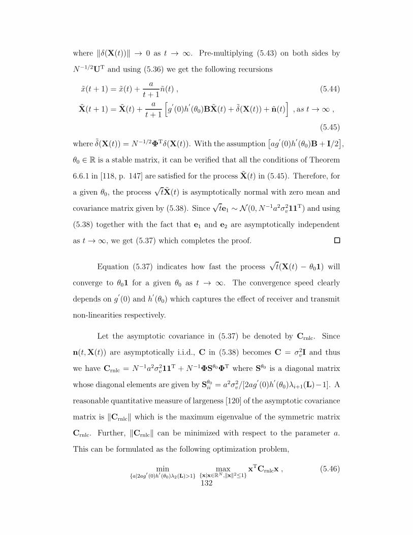
where ‖δ(X(t))‖ → 0 as t → ∞. Pre-multiplying (5.43) on both sides by
N−1/2UT and using (5.36) we get the following recursions
x(t + 1) = x(t) +a
t + 1n(t) , (5.44)
X(t + 1) = X(t) +a
t+ 1
[g
′
(0)h′
(θ0)BX(t) + δ(X(t)) + n(t)], as t → ∞ ,
(5.45)
where δ(X(t)) = N−1/2ΦTδ(X(t)). With the assumption[ag
′
(0)h′
(θ0)B+ I/2],
θ0 ∈ R is a stable matrix, it can be verified that all the conditions of Theorem
6.6.1 in [118, p. 147] are satisfied for the process X(t) in (5.45). Therefore, for
a given θ0, the process√tX(t) is asymptotically normal with zero mean and
covariance matrix given by (5.38). Since√te1 ∼ N (0, N−1a2σ2
v11T) and using
(5.38) together with the fact that e1 and e2 are asymptotically independent
as t → ∞, we get (5.37) which completes the proof.
Equation (5.37) indicates how fast the process√t(X(t) − θ01) will
converge to θ01 for a given θ0 as t → ∞. The convergence speed clearly
depends on g′
(0) and h′
(θ0) which captures the effect of receiver and transmit
non-linearities respectively.
Let the asymptotic covariance in (5.37) be denoted by Crnlc. Since
n(t,X(t)) are asymptotically i.i.d., C in (5.38) becomes C = σ2vI and thus
we have Crnlc = N−1a2σ2v11
T + N−1ΦSθ0ΦT where Sθ0 is a diagonal matrix
whose diagonal elements are given by Sθ0ii = a2σ2
v/[2ag′
(0)h′
(θ0)λi+1(L)−1]. A
reasonable quantitative measure of largeness [120] of the asymptotic covariance
matrix is ‖Crnlc‖ which is the maximum eigenvalue of the symmetric matrix
Crnlc. Further, ‖Crnlc‖ can be minimized with respect to the parameter a.
This can be formulated as the following optimization problem,
min{a|2ag′ (0)h′ (θ0)λ2(L)>1}
max{x|x∈RN ,‖x‖2≤1}
xTCrnlcx , (5.46)
132
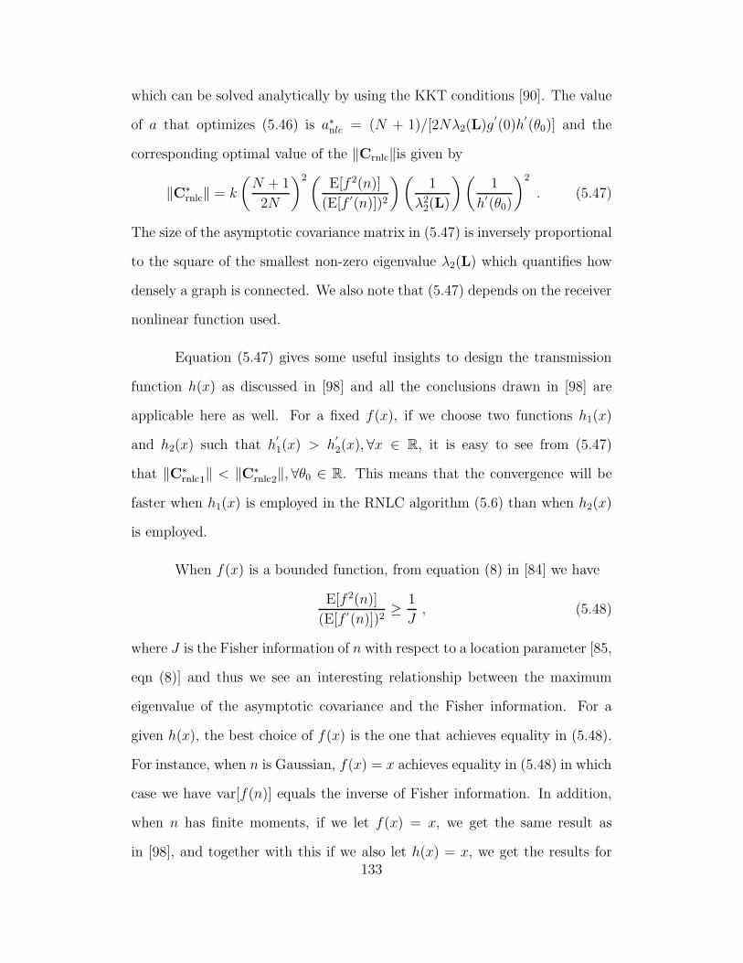
which can be solved analytically by using the KKT conditions [90]. The value
of a that optimizes (5.46) is a∗nlc = (N + 1)/[2Nλ2(L)g′
(0)h′
(θ0)] and the
corresponding optimal value of the ‖Crnlc‖is given by
‖C∗rnlc‖ = k
(N + 1
2N
)2(E[f 2(n)]
(E[f ′(n)])2
)(1
λ22(L)
)(1
h′(θ0)
)2
. (5.47)
The size of the asymptotic covariance matrix in (5.47) is inversely proportional
to the square of the smallest non-zero eigenvalue λ2(L) which quantifies how
densely a graph is connected. We also note that (5.47) depends on the receiver
nonlinear function used.
Equation (5.47) gives some useful insights to design the transmission
function h(x) as discussed in [98] and all the conclusions drawn in [98] are
applicable here as well. For a fixed f(x), if we choose two functions h1(x)
and h2(x) such that h′
1(x) > h′
2(x), ∀x ∈ R, it is easy to see from (5.47)
that ‖C∗rnlc1‖ < ‖C∗
rnlc2‖, ∀θ0 ∈ R. This means that the convergence will be
faster when h1(x) is employed in the RNLC algorithm (5.6) than when h2(x)
is employed.
When f(x) is a bounded function, from equation (8) in [84] we have
E[f 2(n)]
(E[f ′(n)])2≥ 1
J, (5.48)
where J is the Fisher information of n with respect to a location parameter [85,
eqn (8)] and thus we see an interesting relationship between the maximum
eigenvalue of the asymptotic covariance and the Fisher information. For a
given h(x), the best choice of f(x) is the one that achieves equality in (5.48).
For instance, when n is Gaussian, f(x) = x achieves equality in (5.48) in which
case we have var[f(n)] equals the inverse of Fisher information. In addition,
when n has finite moments, if we let f(x) = x, we get the same result as
in [98], and together with this if we also let h(x) = x, we get the results for133
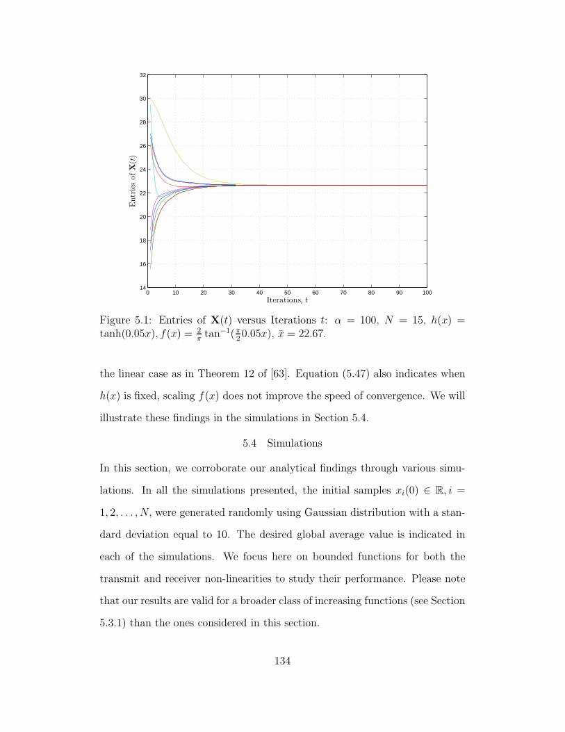
0 10 20 30 40 50 60 70 80 90 10014
16
18
20
22
24
26
28
30
32
Iterations, t
Entr
ies
ofX
(t)
Figure 5.1: Entries of X(t) versus Iterations t: α = 100, N = 15, h(x) =tanh(0.05x), f(x) = 2
πtan−1(π
20.05x), x = 22.67.
the linear case as in Theorem 12 of [63]. Equation (5.47) also indicates when
h(x) is fixed, scaling f(x) does not improve the speed of convergence. We will
illustrate these findings in the simulations in Section 5.4.
5.4 Simulations
In this section, we corroborate our analytical findings through various simu-
lations. In all the simulations presented, the initial samples xi(0) ∈ R, i =
1, 2, . . . , N, were generated randomly using Gaussian distribution with a stan-
dard deviation equal to 10. The desired global average value is indicated in
each of the simulations. We focus here on bounded functions for both the
transmit and receiver non-linearities to study their performance. Please note
that our results are valid for a broader class of increasing functions (see Section
5.3.1) than the ones considered in this section.
134
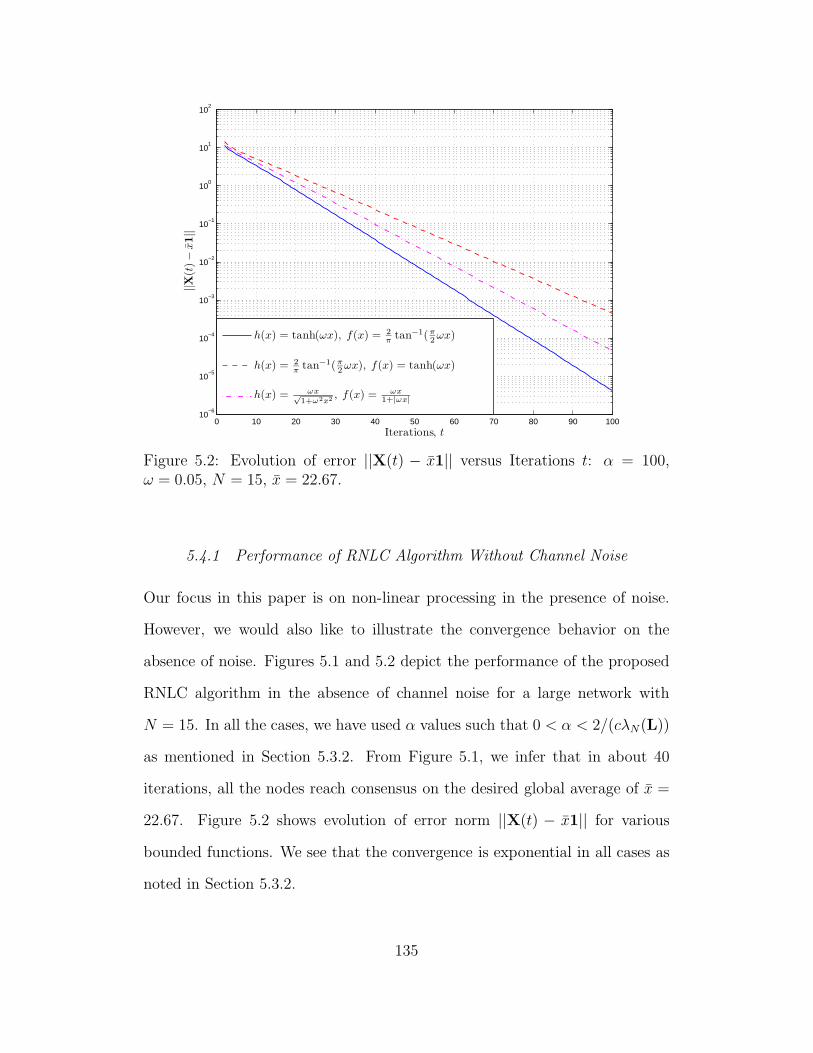
0 10 20 30 40 50 60 70 80 90 10010
−6
10−5
10−4
10−3
10−2
10−1
100
101
102
Iterations, t
||X(t
)−
x1||
h(x) = tanh(ωx), f(x) = 2
πtan−1(π
2ωx)
h(x) = 2
πtan−1(π
2ωx), f(x) = tanh(ωx)
h(x) = ωx√1+ω2x2
, f(x) = ωx
1+|ωx|
Figure 5.2: Evolution of error ||X(t) − x1|| versus Iterations t: α = 100,ω = 0.05, N = 15, x = 22.67.
5.4.1 Performance of RNLC Algorithm Without Channel Noise
Our focus in this paper is on non-linear processing in the presence of noise.
However, we would also like to illustrate the convergence behavior on the
absence of noise. Figures 5.1 and 5.2 depict the performance of the proposed
RNLC algorithm in the absence of channel noise for a large network with
N = 15. In all the cases, we have used α values such that 0 < α < 2/(cλN(L))
as mentioned in Section 5.3.2. From Figure 5.1, we infer that in about 40
iterations, all the nodes reach consensus on the desired global average of x =
22.67. Figure 5.2 shows evolution of error norm ||X(t) − x1|| for various
bounded functions. We see that the convergence is exponential in all cases as
noted in Section 5.3.2.
135
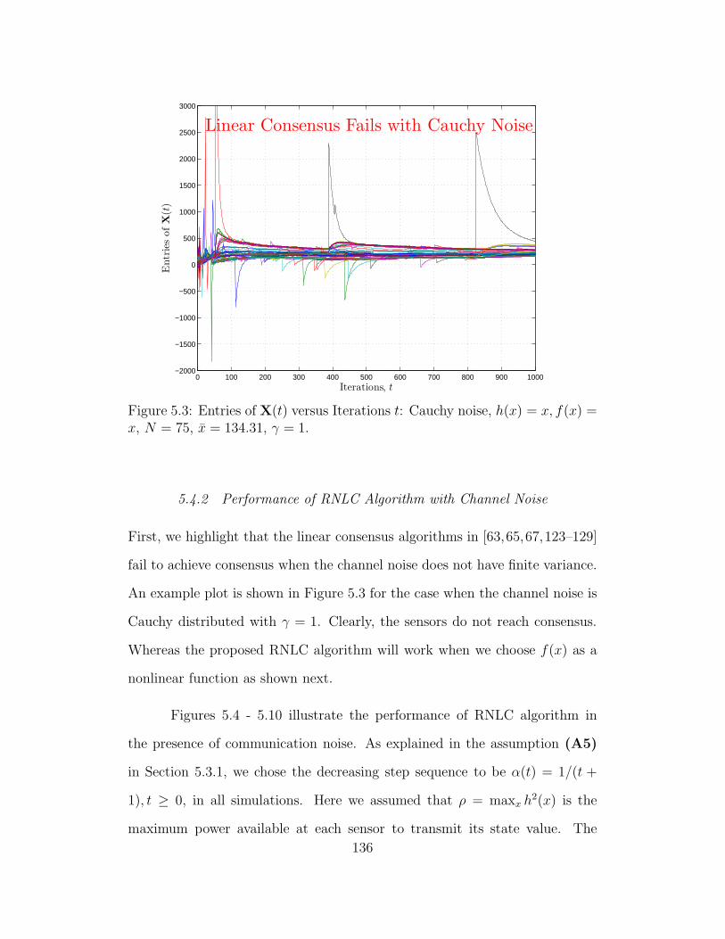
0 100 200 300 400 500 600 700 800 900 1000−2000
−1500
−1000
−500
0
500
1000
1500
2000
2500
3000
Iterations, t
Entr
ies
ofX
(t)
Linear Consensus Fails with Cauchy Noise
Figure 5.3: Entries of X(t) versus Iterations t: Cauchy noise, h(x) = x, f(x) =x, N = 75, x = 134.31, γ = 1.
5.4.2 Performance of RNLC Algorithm with Channel Noise
First, we highlight that the linear consensus algorithms in [63,65,67,123–129]
fail to achieve consensus when the channel noise does not have finite variance.
An example plot is shown in Figure 5.3 for the case when the channel noise is
Cauchy distributed with γ = 1. Clearly, the sensors do not reach consensus.
Whereas the proposed RNLC algorithm will work when we choose f(x) as a
nonlinear function as shown next.
Figures 5.4 - 5.10 illustrate the performance of RNLC algorithm in
the presence of communication noise. As explained in the assumption (A5)
in Section 5.3.1, we chose the decreasing step sequence to be α(t) = 1/(t +
1), t ≥ 0, in all simulations. Here we assumed that ρ = maxx h2(x) is the
maximum power available at each sensor to transmit its state value. The
136
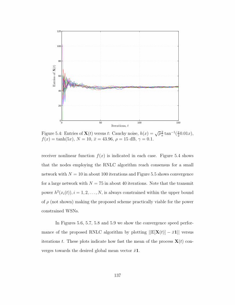
0 50 100 1500
20
40
60
80
100
120
Iterations, t
Entr
ies
ofX
(t)
Figure 5.4: Entries of X(t) versus t: Cauchy noise, h(x) =√ρ 2πtan−1(π
20.01x),
f(x) = tanh(5x), N = 10, x = 43.96, ρ = 15 dB, γ = 0.1.
receiver nonlinear function f(x) is indicated in each case. Figure 5.4 shows
that the nodes employing the RNLC algorithm reach consensus for a small
network with N = 10 in about 100 iterations and Figure 5.5 shows convergence
for a large network with N = 75 in about 40 iterations. Note that the transmit
power h2(xi(t)), i = 1, 2, . . . , N, is always constrained within the upper bound
of ρ (not shown) making the proposed scheme practically viable for the power
constrained WSNs.
In Figures 5.6, 5.7, 5.8 and 5.9 we show the convergence speed perfor-
mance of the proposed RNLC algorithm by plotting ||E[X(t)] − x1|| versus
iterations t. These plots indicate how fast the mean of the process X(t) con-
verges towards the desired global mean vector x1.
137
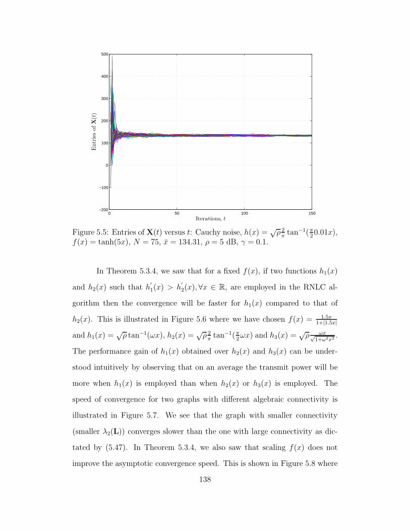
0 50 100 150−200
−100
0
100
200
300
400
500
Iterations, t
Entr
ies
ofX
(t)
Figure 5.5: Entries of X(t) versus t: Cauchy noise, h(x) =√ρ 2πtan−1(π
20.01x),
f(x) = tanh(5x), N = 75, x = 134.31, ρ = 5 dB, γ = 0.1.
In Theorem 5.3.4, we saw that for a fixed f(x), if two functions h1(x)
and h2(x) such that h′
1(x) > h′
2(x), ∀x ∈ R, are employed in the RNLC al-
gorithm then the convergence will be faster for h1(x) compared to that of
h2(x). This is illustrated in Figure 5.6 where we have chosen f(x) = 1.5x1+|1.5x|
and h1(x) =√ρ tan−1(ωx), h2(x) =
√ρ 2πtan−1(π
2ωx) and h3(x) =
√ρ ωx√
1+ω2x2.
The performance gain of h1(x) obtained over h2(x) and h3(x) can be under-
stood intuitively by observing that on an average the transmit power will be
more when h1(x) is employed than when h2(x) or h3(x) is employed. The
speed of convergence for two graphs with different algebraic connectivity is
illustrated in Figure 5.7. We see that the graph with smaller connectivity
(smaller λ2(L)) converges slower than the one with large connectivity as dic-
tated by (5.47). In Theorem 5.3.4, we also saw that scaling f(x) does not
improve the asymptotic convergence speed. This is shown in Figure 5.8 where
138
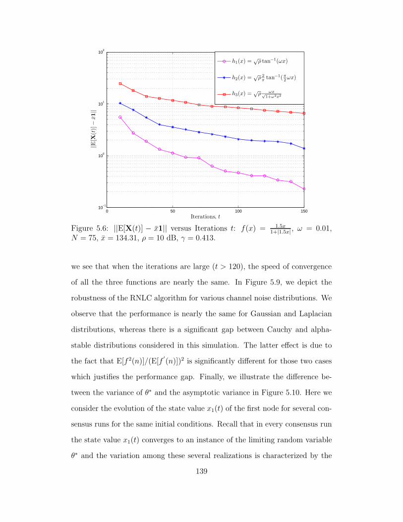
0 50 100 15010
−1
100
101
102
Iterations, t
||E[X
(t)]−
x1||
h1(x) =√
ρ tan−1(ωx)
h2(x) =√
ρ 2
πtan−1(π
2ωx)
h3(x) =√
ρ ωx√1+ω2x2
Figure 5.6: ||E[X(t)] − x1|| versus Iterations t: f(x) = 1.5x1+|1.5x| , ω = 0.01,
N = 75, x = 134.31, ρ = 10 dB, γ = 0.413.
we see that when the iterations are large (t > 120), the speed of convergence
of all the three functions are nearly the same. In Figure 5.9, we depict the
robustness of the RNLC algorithm for various channel noise distributions. We
observe that the performance is nearly the same for Gaussian and Laplacian
distributions, whereas there is a significant gap between Cauchy and alpha-
stable distributions considered in this simulation. The latter effect is due to
the fact that E[f 2(n)]/(E[f′
(n)])2 is significantly different for those two cases
which justifies the performance gap. Finally, we illustrate the difference be-
tween the variance of θ∗ and the asymptotic variance in Figure 5.10. Here we
consider the evolution of the state value x1(t) of the first node for several con-
sensus runs for the same initial conditions. Recall that in every consensus run
the state value x1(t) converges to an instance of the limiting random variable
θ∗ and the variation among these several realizations is characterized by the
139
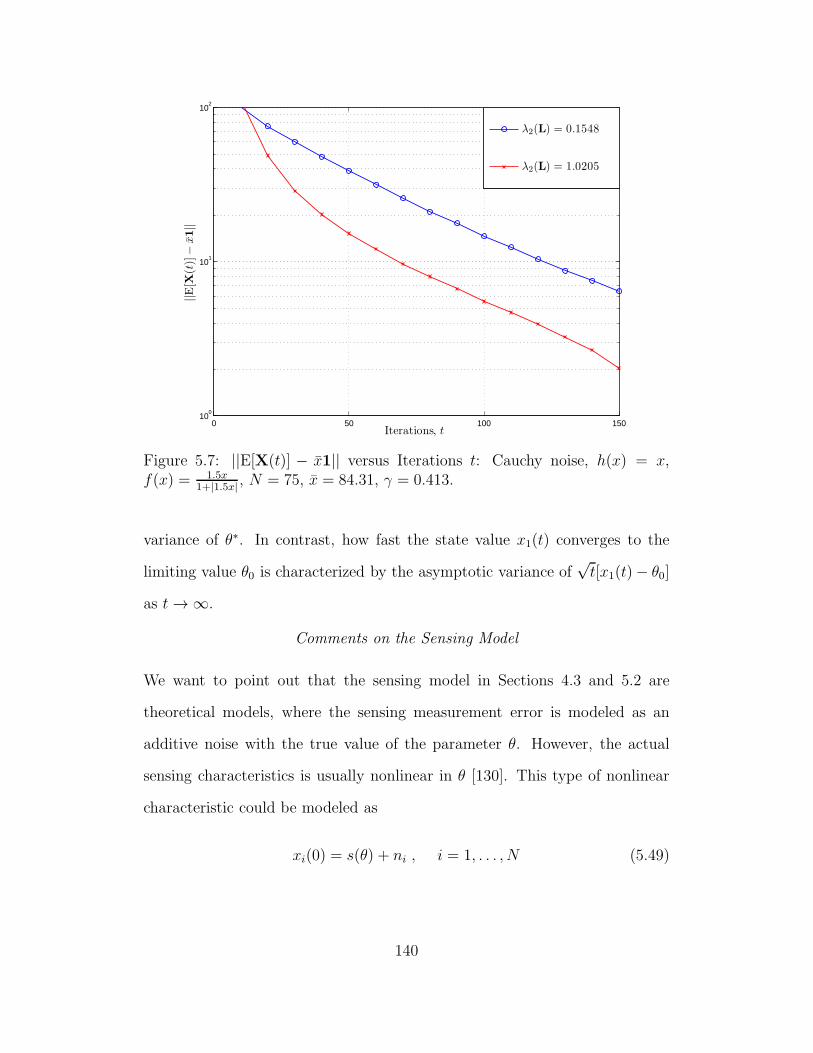
0 50 100 15010
0
101
102
Iterations, t
||E[X
(t)]−
x1||
λ2(L) = 0.1548
λ2(L) = 1.0205
Figure 5.7: ||E[X(t)] − x1|| versus Iterations t: Cauchy noise, h(x) = x,f(x) = 1.5x
1+|1.5x| , N = 75, x = 84.31, γ = 0.413.
variance of θ∗. In contrast, how fast the state value x1(t) converges to the
limiting value θ0 is characterized by the asymptotic variance of√t[x1(t)− θ0]
as t → ∞.
Comments on the Sensing Model
We want to point out that the sensing model in Sections 4.3 and 5.2 are
theoretical models, where the sensing measurement error is modeled as an
additive noise with the true value of the parameter θ. However, the actual
sensing characteristics is usually nonlinear in θ [130]. This type of nonlinear
characteristic could be modeled as
xi(0) = s(θ) + ni , i = 1, . . . , N (5.49)
140
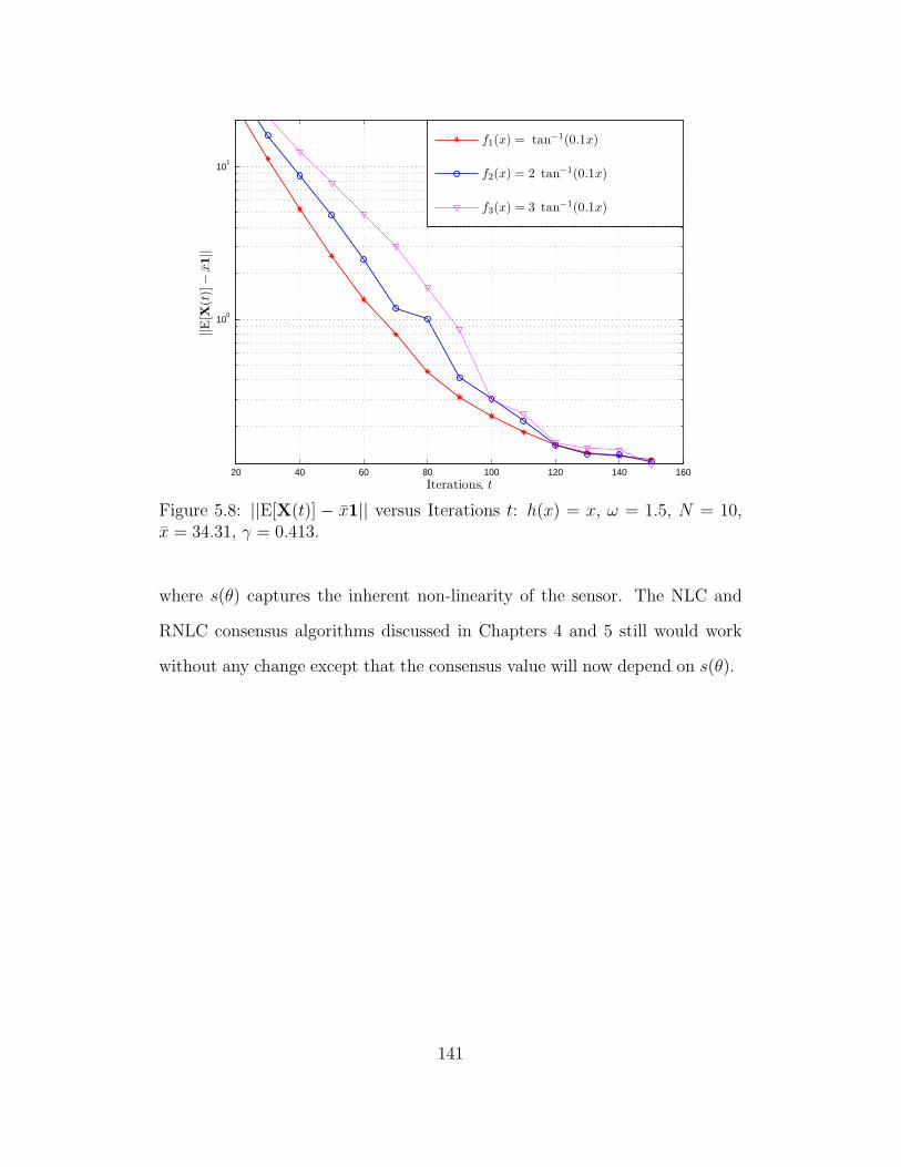
20 40 60 80 100 120 140 160
100
101
Iterations, t
||E[X
(t)]−
x1||
f1(x) = tan−1(0.1x)
f2(x) = 2 tan−1(0.1x)
f3(x) = 3 tan−1(0.1x)
Figure 5.8: ||E[X(t)] − x1|| versus Iterations t: h(x) = x, ω = 1.5, N = 10,x = 34.31, γ = 0.413.
where s(θ) captures the inherent non-linearity of the sensor. The NLC and
RNLC consensus algorithms discussed in Chapters 4 and 5 still would work
without any change except that the consensus value will now depend on s(θ).
141
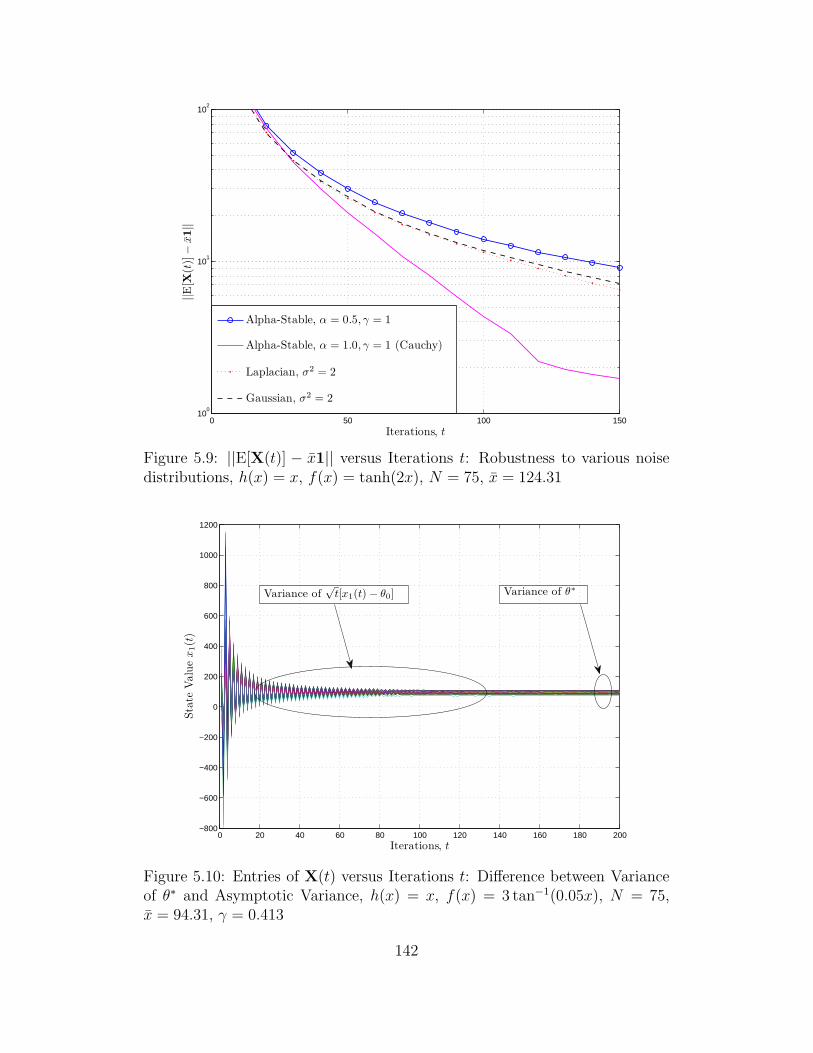
0 50 100 15010
0
101
102
Iterations, t
||E[X
(t)]−
x1||
Alpha-Stable, α = 0.5, γ = 1
Alpha-Stable, α = 1.0, γ = 1 (Cauchy)
Laplacian, σ2 = 2
Gaussian, σ2 = 2
Figure 5.9: ||E[X(t)] − x1|| versus Iterations t: Robustness to various noisedistributions, h(x) = x, f(x) = tanh(2x), N = 75, x = 124.31
0 20 40 60 80 100 120 140 160 180 200−800
−600
−400
−200
0
200
400
600
800
1000
1200
Iterations, t
Sta
teV
alu
ex
1(t
)
Variance of√
t[x1(t) − θ0] Variance of θ∗
Figure 5.10: Entries of X(t) versus Iterations t: Difference between Varianceof θ∗ and Asymptotic Variance, h(x) = x, f(x) = 3 tan−1(0.05x), N = 75,x = 94.31, γ = 0.413
142
Chapter 6
Conclusions
In Chapter 2 of this dissertation, a distributed detection scheme relying on
constant modulus transmissions from the sensors is proposed over a Gaussian
multiple access channel. The instantaneous transmit power does not depend
on the random sensing noise, which is a desirable feature for low-power sen-
sors with limited peak power capabilities. The DC of the proposed scheme
is shown to depend on the characteristic function of the sensing noise and
optimized with respect to ω for various sensing noise distributions. In addi-
tion to the desirable constant-power feature, the proposed detector is robust
to impulsive noise, and performs well even when the moments of the sensing
noise do not exist as in the case of the Cauchy distribution. Extensions to
non-homogeneous sensors with non-identically distributed noise are also con-
sidered. It is shown that over Gaussian multiple access channels, the proposed
detector outperforms AF, DF and MDF schemes consistently, and the MAF
scheme when the sensing SNR is greater than 4 dB. The proposed detector
is shown to work with the non-Gaussian channel noises as well. The error
exponent is also derived for the proposed scheme and large deviation theory
is used to approximate Pe(ω) for large L. It is shown that while the DC has
a simpler expression for the purpose of optimizing ω, the probability of error
approximation based on (2.40) is shown to be an accurate indicator of detec-
tion performance for all distributions and moderate number of sensors. The
effect of fading is also considered, and shown to be detrimental to the detection
performance.
In Chapter 3, the more general problem of a distributed inference
scheme using bounded transmissions from the sensors over Gaussian multi-
143
ple access channels is considered. A distributed inference scheme relying on
bounded transmissions from the sensors is considered over Gaussian multi-
ple access channels. The instantaneous transmit power is always constrained
to be bounded irrespective of the random sensing noise, which is a desirable
feature for low-power sensors with limited peak power capabilities. For the
distributed estimation problem, the estimation scheme using bounded trans-
missions is shown to be strongly consistent provided that the variance of the
noise samples are bounded and that the transmission function is one-to-one.
For sensing noise distributions for which the sample mean is highly subopti-
mal or inconsistent, the proposed estimator is shown to be consistent. For
heavy-tailed distributions with infinite variance like Cauchy, it is shown that
the AF scheme fails, and that the proposed approach is superior to AF. As
long as the variance of the noise samples grow to infinity slower than linearly,
AF scheme is consistent, whereas the proposed scheme fails when the variance
of the noise samples go to infinity at any rate. For the distributed detection
problem, the regimes under which reliable detection is possible or impossible
are also established. Monte Carlo simulations are presented to illustrate the
performance of several bounded transmission functions for a variety of sensing
noise distributions.
In Chapter 4 of this dissertation, a distributed consensus algorithm in
which every sensor maps its state value through a bounded function before
transmission to constrain the transmit power is proposed. The transmitted
signal power at every node in every iteration is always bounded irrespective
of the state value or the communication noise, which is a desirable feature
for low-power sensors with limited peak power capabilities. In the presence
of communication noise, it is proved using the theory of Markov processes
144
that the sensors reach consensus asymptotically on a finite random variable
whose expectation contains the desired sample average of the initial sensor
measurements, and whose mean-squared error is bounded. The asymptotic
convergence speed of the proposed algorithm is characterized by deriving the
asymptotic covariance matrix using results from stochastic approximation the-
ory. While the proposed NLC algorithm has the desirable feature of bounded
transmit power, it is shown that using the best case NLC algorithm results
in larger asymptotic covariance compared to the best case linear consensus
algorithm. In the absence of communication noise, it is illustrated that the
network achieves consensus on the global sample average exponentially fast
provided the step size is chosen appropriately and that by adjusting the step
size, it is possible to achieve the same speed of convergence as that of the best
case linear consensus algorithm using Laplacian heuristic.
Finally, in Chapter 5, a distributed average consensus algorithm in
which every sensor performs a nonlinear processing at the receiver is pro-
posed. Every sensor also maps its state value through a bounded function
before transmission to constrain the transmit power. It is shown that non-
linearity at the receiver nodes makes the algorithm robust to a wide range of
channel noise distributions including the impulsive ones. The proposed algo-
rithm does not need the requirement of finite moments on the communication
noise and thus it is proved to be not only more general than the existing
consensus algorithms but is practically viable for WSNs deployed in adverse
conditions. It is proved using the theory of Markov processes that the sensors
reach consensus asymptotically on a finite random variable whose expectation
contains the desired sample average of the initial sensor measurements, and
whose mean-squared error is bounded. The asymptotic convergence speed of
145

the proposed algorithm is characterized by deriving the asymptotic covariance
matrix using results from stochastic approximation theory. It is shown that
scaling the receiver nonlinear function does not affect the convergence speed
of the proposed algorithm and its robustness to a variety of channel noise
distributions is highlighted. An interesting relationship between the Fisher in-
formation and the asymptotic covariance matrix is also shown. In the absence
of communication noise, it is illustrated that the network achieves consensus
on the global sample average exponentially fast provided the step size is chosen
appropriately.
146
REFERENCES
[1] B. Sadler, “Fundamentals of energy-constrained sensor network sys-tems,” Aerospace and Electronic Systems Magazine, IEEE, vol. 20, no. 8,pp. 17–35, Aug. 2005.
[2] I. F. Akyildiz, W. Su, Y. Sankarasubramaniam, and E. Cayirci, “A sur-vey on sensor networks,” IEEE Communication Magazine, pp. 102–114,August 2002.
[3] G. J. Pottie and W. J. Kaiser, “Wireless integrated network sensors,”Communications of the ACM, vol. 43, no. 5, p. pp. 5158, May 2000.
[4] B. Warneke, M. Last, B. Liebowitz, and K. S. J. Pister, “Smart dust:communicating with a cubic-millimeter computer,” Computer, vol. 34,no. 1, pp. 44–51, January 2001.
[5] M. K. Banavar, “Distributed inference over multiple-access channelswith wireless sensor networks,” Ph.D. dissertation, School of Electrical,Computer and Energy Engineering, Arizona State University, 2010.
[6] S. M. Kay, Fundamentals of Statistical Signal Processing: Detection The-ory. New Jersey: Prentice Hall, 1998.
[7] ——, Fundamentals of Statistical Signal Processing: Estimation Theory.New Jersey: Prentice Hall, 1998.
[8] S. Y. Chueng, S. C. Ergen, and P. Varaiya, “Traffic surveillance withwireless magnetic sensors,” Proceedings of the 12th ITS World Congress,November 2005.
[9] L. Kleinrock and J. Silvester, “Optimum transmission radii for packetradio networks or why six is a magic number,” in NTC ’78; Na-tional Telecommunications Conference, Birmingham, Ala., December 3-6, 1978, Conference Record. Volume 1. (A79-40501 17-32) Piscataway,N.J., Institute of Electrical and Electronics Engineers, Inc., 1978, p.4.3.1-4.3.5., vol. 1, 1978, pp. 4.3.1–4.3.5.
[10] P. Gupta and P. R. Kumar, Critical Power for Asymptotic Connectivityin Wireless Networks. Birkhauser, 1998.
147
[11] O. Dousse, P. Thiran, and M. Hasler, “Connectivity in ad-hoc and hybridnetworks,” IEEE Infocom, pp. 1079–1088, 2002.
[12] F. Xue and P. R. Kumar, The Number of Neighbors Needed for Con-nectivity of Wireless Networks. The Netherlands: Kluwer AcademicPublishers, 2004, ch. 10, pp. 169–181.
[13] O. Dousse, F. Baccelli, and P. Thiran, “Impact of interferences on con-nectivity in ad-hoc networks,” IEEE/ACM Transactions on Networking,vol. 13, no. 2, pp. 425–436, April 2005.
[14] P. Gupta and P. R. Kumar, “The capacity of wireless networks,” IEEETransactions on Information Theory, vol. 46, no. 2, pp. 388–404, March2000.
[15] M. Grossglauser and D. Tse, “Mobility increases the capacity of ad-hocwireless networks,” IEEE Infocom, pp. 1360–1369, 2001.
[16] H. E. Gamal, “On the scaling laws of dense wireless sensor networks,”Proceedings of the Annual Allerton Conference on Communication, Con-trol and Coding, vol. 41, no. 3, pp. 1393–1401, 2003.
[17] F. Xue, L. Xie, and P. R. Kumar, “The transport capacity of wire-less networks over fading channels,” IEEE Transactions on InformationTheory, vol. 51, no. 3, pp. 834–847, March 2005.
[18] L.-L. Xie and P. Kumar, “On the path-loss attenuation regime for posi-tive cost and linear scaling of transport capacity in wireless networks,”IEEE Transactions on Information Theory, vol. 52, no. 6, pp. 2313–2328,June 2006.
[19] F. Xue and P. Kumar, Scaling Laws for Ad-Hoc Wireless Networks: AnInformation Theoretic Approach. Now Publishers, 2006, vol. 1, no. 2,pp. 145–270.
[20] M. Bohge andW. Trappe, “An authentication framework for hierarchicalad-hoc sensor networks. new york: Acm, 2003,” Proceedings of the 2ndACM workshop on Wireless security, vol. 22, no. 2, p. 7987, 2003.
[21] L. Sankaranarayanan, G. Kramer, and N. Mandayam, “Hierarchical sen-sor networks: capacity bounds and cooperative strategies using the
148
multiple-access relay channel model,” in Sensor and Ad-Hoc Commu-nications and Networks, 2004. IEEE SECON 2004. 2004 First AnnualIEEE Communications Society Conference on, oct. 2004, pp. 191 – 199.
[22] R. Viswanathan and P. Varshney, “Distributed detection with multiplesensors Part I: Fundamentals,” Proceedings of the IEEE, vol. 85, no. 1,pp. 54–63, Jan 1997.
[23] R. Blum, S. Kassam, and H. Poor, “Distributed detection with multiplesensors Part II: Advanced topics,” Proceedings of the IEEE, vol. 85,no. 1, pp. 64 –79, jan 1997.
[24] M. Gastpar and M. Vetterli, “Source-channel communication in sensornetworks,” Proceedings of the 2nd International Workshop on Informa-tion Processing in Sensor Networks (IPSN’03), pp. 162–177, April 2003.
[25] M. Banavar, C. Tepedelenlioglu, and A. Spanias, “Estimation over fad-ing channels with limited feedback using distributed sensing,” SignalProcessing, IEEE Transactions on, vol. 58, no. 1, pp. 414 –425, jan.2010.
[26] G. Mergen and L. Tong, “Type based estimation over multiaccess chan-nels,” IEEE Transactions on Signal Processing, vol. 54, no. 2, pp. 613–626, February 2006.
[27] J.-J. Xiao and Z.-Q. Luo, “Universal decentralized detection in abandwidth-constrained sensor network,” IEEE Transactions on SignalProcessing, vol. 53, no. 8, pp. 2617 – 2624, August 2005.
[28] Z. Hu and B. Li, “On the fundamental capacity and lifetime limits ofenergy-constrained wireless sensor networks,” in Proc. 10th IEEE Real-Time and Embedded Technology and Applications Symposium RTAS2004, May 25–28, 2004, pp. 2–9.
[29] M. Bhardwaj and A. P. Chandrakasan, “Bounding the lifetime of sensornetworks via optimal role assignments,” in Proc. IEEE Twenty-FirstAnnual Joint Conference of the IEEE Computer and CommunicationsSocieties INFOCOM 2002, vol. 3, Jun. 23–27, 2002, pp. 1587–1596.
149
[30] M. Bhardwaj, T. Garnett, and A. P. Chandrakasan, “Upper bounds onthe lifetime of sensor networks,” in Proc. IEEE International Conferenceon Communications ICC 2001, vol. 3, Jun. 11–14, 2001, pp. 785–790.
[31] K. Kalpakis and S. Tang, “A combinatorial algorithm for the maximumlifetime data gathering and aggregation problem in sensor networks,”in Proc. International Symposium on a World of Wireless, Mobile andMultimedia Networks WoWMoM 2008, Jun. 23–26, 2008, pp. 1–8.
[32] J. L. Gao, “Analysis of energy consumption for ad-hoc wireless sensornetworks using a bit-meter-per-joule metric.” in IPN Progress Report42-150, Jet Propulsion Laboratory, vol. 3, Aug 2002, pp. 785–790.
[33] S. E, I. N. Cho S-H and, M. R, S. A, W. A, and C. A, “Physical layerdriven protocol and algorithm design for energy-efficient wireless sensornetworks,” in In Proceedings of 7th ACM Conference on Mobile Com-puting and Networkin, July 2001.
[34] P. K. Varshney, Distributed Detection and Data Fusion. New York:Springer, 1997.
[35] J. Tsitsiklis, “Decentralized detection,” Advances in Statistical SignalProcessing, vol. 2, pp. 297–344, March 1993.
[36] F. Li and J. S. Evans, “Optimal strategies for distributed detectionover multiaccess channels,” in Proc. IEEE International Conference onAcoustics, Speech and Signal Processing ICASSP 2008, Mar. 2008, pp.2417–2420.
[37] ——, “Design of distributed detection schemes for multiaccess channels,”in Proc. Australian Communications Theory Workshop AusCTW 2008,Jan. 2008, pp. 51–57.
[38] C. Tepedelenlioglu and A. Narasimhamurthy, “Distributed estimationwith constant modulus signaling over multiple access channels,” in Proc.IEEE International Conference on Acoustics, Speech and Signal Process-ing ICASSP 2010, Mar. 2010.
[39] G. S. Lauer and N. R. S. Jr, “Distributed detection of known signalin correlated noise,” Rep. ALPHATECH, Burlington, MA, vol. 2, pp.297–344, March 1982.
150
[40] A. R. Reibman, “Performance and fault-tolerance of distributed detec-tion networks,,” Ph.D. dissertation, Dept. Electrical Engineering, DukeUniv, Durham, 1987.
[41] M. Xiang and C. Han, “Optimization of distributed detection networkswith tree structures,” in Information Fusion, 2002. Proceedings of theFifth International Conference on, vol. 1, 2002, pp. 164–169 vol.1.
[42] C. Tepedelenlioglu and A. Narasimhamurthy, “Universal distributed es-timation over multiple access channels with constant modulus signaling,”Signal Processing, IEEE Transactions on, vol. 58, no. 9, pp. 4783 –4794,Sept. 2010.
[43] M. Banavar, C. Tepedelenlioglu, and A. Spanias, “Distributed SNR esti-mation using constant modulus signaling over Gaussian multiple-accesschannels,” in Digital Signal Processing Workshop and IEEE Signal Pro-cessing Education Workshop (DSP/SPE), 2011 IEEE, jan. 2011, pp. 24–29.
[44] ——, “Distributed SNR estimation with power constrained signalingover Gaussian multiple-access channels,” Signal Processing, IEEE Trans-actions on, vol. PP, no. 99, p. 1, 2012.
[45] J. Tsitsiklis, “Decentralized detection by a large number of sensors,”Mathematics of Control, Signals, and Systems, vol. 2, pp. 167–182, April1988.
[46] G. Mergen, V. Naware, and L. Tong, “Asymptotic detection performanceof type-based multiple access in sensor networks,” in Signal ProcessingAdvances in Wireless Communications, 2005 IEEE 6th Workshop on,June 2005, pp. 1018–1022.
[47] F. D. Hollander, Large Deviations (Fields Institute Monographs,14).New York: Amer. Math. Soc., 2000.
[48] J.-J. Xiao, A. Ribeiro, Z.-Q. Luo, and G. Giannakis, “Distributedcompression-estimation using wireless sensor networks,” IEEE SignalProcessing Magazine, vol. 23, no. 4, pp. 27–41, July 2006.
[49] J.-J. Xiao, S. Cui, Z.-Q. Luo, and A. J. Goldsmith, “Joint estimationin sensor networks under energy constraints,” Poceedings of the First
151
Annual IEEE Communications Society Conference on Sensor and Ad-Hoc Communications and Networks, pp. 264–271, October 2004.
[50] S. Cui, J. Xiao, A. J. Goldsmith, Z.-Q. Luo, and H. V. Poor, “Energy-efficient joint estimation in sensor networks - analog vs. digital,” in Pro-ceedings of the IEEE International Conference on Acoustics, Speech andSignal Processing, vol. 4, March 2005, pp. 745–748.
[51] S. Cui, J.-J. Xiao, A. J. Goldsmith, Z.-Q. Luo, and H. V. Poor, “Esti-mation diversity and energy efficiency in distributed sensing,” vol. 55,no. 9, pp. 4683–4695, Sep. 2007.
[52] J.-J. Xiao, S. Cui, Z.-Q. Luo, and A. J. Goldsmith, “Power schedulingof universal decentralized estimation in sensor networks,” IEEE Trans-actions on Signal Processing, vol. 54, no. 2, pp. 413–422, February 2006.
[53] Z.-Q. Luo, “Universal decentralized estimation in a bandwidth con-strained sensor network,” IEEE Transactions on Information Theory,vol. 51, no. 6, pp. 2210–2219, June 2005.
[54] P. Gao and C. Tepedelenliglu, “Practical issues in estimation over mul-tiaccess fading channels with TBMA wireless sensor networks,” vol. 56,no. 3, pp. 1217–1229, Mar. 2008.
[55] J. Xiao, S. Cui, Z.-Q. Luo, and A. Goldsmith, “CTH15-1: Linear Co-herent Decentralized Estimation,” GLOBECOM ’06. IEEE, pp. 1–5,November 2006.
[56] J. N. Tsitsiklis, “Problems in decision making and com-putation,” Department of Electrical Engineering and Com-puter Science, MIT, Cambridge, MA, 1984. [Online]. Available:http://www.mit.edu/ jnt/Papers/PhD-84-jnt.pdf
[57] J. Tsitsiklis and M. Athans, “Convergence and asymptotic agreement indistributed decision problems,” Automatic Control, IEEE Transactionson, vol. 29, no. 1, pp. 42 – 50, Jan. 1984.
[58] L. Xiao and S. Boyd, “Fast linear iterations for distributed averaging,”in Decision and Control, 2003. Proceedings. 42nd IEEE Conference on,vol. 5, Dec. 2003, pp. 4997 – 5002.
152
[59] S. Boyd, A. Ghosh, B. Prabhakar, and D. Shah, “Analysis and optimiza-tion of randomized gossip algorithms,” in Decision and Control, 2004.CDC. 43rd IEEE Conference on, vol. 5, Dec. 2004, pp. 5310 – 5315.
[60] R. Saber and R. Murray, “Consensus protocols for networks of dynamicagents,” in American Control Conference, 2003. Proceedings of the 2003,vol. 2, Apr. 2003, pp. 951 – 956.
[61] R. Olfati-Saber, J. Fax, and R. Murray, “Consensus and cooperation innetworked multi-agent systems,” Proceedings of the IEEE, vol. 95, no. 1,pp. 215 –233, Jan. 2007.
[62] R. Olfati-Saber and R. Murray, “Consensus problems in networks ofagents with switching topology and time-delays,” Automatic Control,IEEE Transactions on, vol. 49, no. 9, pp. 1520 – 1533, Sept. 2004.
[63] M. Huang and J. Manton, “Stochastic consensus seeking with measure-ment noise: Convergence and asymptotic normality,” in American Con-trol Conference, 2008, June 2008, pp. 1337 –1342.
[64] B. Oreshkin, T. Aysal, and M. Coates, “Distributed average consensuswith increased convergence rate,” in Acoustics, Speech and Signal Pro-cessing, 2008. ICASSP 2008. IEEE International Conference on, Mar.2008, pp. 2285 –2288.
[65] S. Kar and J. Moura, “Distributed consensus algorithms in sensor net-works with imperfect communication: Link failures and channel noise,”Signal Processing, IEEE Transactions on, vol. 57, no. 1, pp. 355 –369,Jan. 2009.
[66] S. Kar, S. Aldosari, and J. Moura, “Topology for distributed inferenceon graphs,” Signal Processing, IEEE Transactions on, vol. 56, no. 6, pp.2609 –2613, June 2008.
[67] S. Kar and J. Moura, “Distributed average consensus in sensor networkswith random link failures and communication channel noise,” in Signals,Systems and Computers, 2007. ACSSC 2007. Conference Record of theForty-First Asilomar Conference on, Nov. 2007, pp. 676 –680.
153
[68] T. Duman and M. Salehi, “Decentralized detection over multiple-accesschannels,” Aerospace and Electronic Systems, IEEE Transactions on,vol. 34, no. 2, pp. 469 –476, apr 1998.
[69] W. Li and H. Dai, “Distributed detection in wireless sensor networksusing a multiple access channel,” Signal Processing, IEEE Transactionson, vol. 55, no. 3, pp. 822 –833, march 2007.
[70] K. Liu and A. Sayeed, “Type-based decentralized detection in wirelesssensor networks,” Signal Processing, IEEE Transactions on, vol. 55,no. 5, pp. 1899–1910, May 2007.
[71] G. Mergen, V. Naware, and L. Tong, “Asymptotic detection performanceof type-based multiple access over multiaccess fading channels,” SignalProcessing, IEEE Transactions on, vol. 55, no. 3, pp. 1081–1092, March2007.
[72] A. Anandkumar and L. Tong, “Type-based random access for distributeddetection over multiaccess fading channels,” Signal Processing, IEEETransactions on, vol. 55, no. 10, pp. 5032–5043, Oct. 2007.
[73] T. M. Cover and J. A. Thomas, Elements of Information Theory. NewYork: Wiley, 1991.
[74] Q. Tian and E. J. Coyle, “Optimal distributed detection in clusteredwireless sensor networks,” IEEE Transactions on Signal Processing,vol. 55, no. 7, pp. 3892–3904, 2007.
[75] F. Li and J. S. Evans, “Decision fusion over noncoherent fading multi-access channels,” in Proc. IEEE Global Telecommunications ConferenceIEEE GLOBECOM 2008, Nov. 2008, pp. 1–5.
[76] M. Banavar, A. Smith, C. Tepedelenlioglu, and A. Spanias, “Distributeddetection over fading MACs with multiple antennas at the fusion cen-ter,” in Acoustics Speech and Signal Processing (ICASSP), 2010 IEEEInternational Conference on, march 2010, pp. 2894 –2897.
[77] T. Aysal and K. Barner, “Constrained decentralized estimation overnoisy channels for sensor networks,” Signal Processing, IEEE Transac-tions on, vol. 56, no. 4, pp. 1398 –1410, 2008.
154
[78] J.-J. Xiao, S. Cui, Z.-Q. Luo, and A. Goldsmith, “Linear coherent decen-tralized estimation,” Signal Processing, IEEE Transactions on, vol. 56,no. 2, pp. 757 –770, 2008.
[79] B. Picinbono, “On deflection as a performance criterion in detection,”Aerospace and Electronic Systems, IEEE Transactions on, vol. 31, no. 3,pp. 1072 –1081, jul 1995.
[80] R. Niu and P. Varshney, “Performance analysis of distributed detectionin a random sensor field,” Signal Processing, IEEE Transactions on,vol. 56, no. 1, pp. 339 –349, jan. 2008.
[81] H. V. Poor, An Introduction to Signal Detection and Estimation. NewYork: Springer-Verlag, 1994.
[82] S. A. Kassam, Signal Detection in Non-Gaussian Noise. Springer; 1edition, 1987.
[83] G. Samorodnitsky and M. S. Taqqu, “Stable non-Gaussian random pro-cesses,” 1994, pp. 2–4, 10–13, 77–79, 84–86.
[84] Z. Zhang, “Inequalities for characteristic functions involving Fisher in-formation,” Comptes Rendus Mathematique, vol. 344, no. 5, pp. 327–330,March 2007.
[85] R. Zamir, “A proof of the Fisher information inequality via a data pro-cessing argument,” Information Theory, IEEE Transactions on, vol. 44,no. 3, pp. 1246–1250, May 1998.
[86] B. Porat, Digital processing of random signals: theory and methods.Prentice-Hall, Englewood Cliffs, NJ, 1994.
[87] N. G. Ushakov, Selected topics in characteristic functions. VSP Inter-national Science Publishers, 1999.
[88] J. A. Bucklew, Large Deviation Techniques in Decision, Simulation, andEstimation. Wiley-Interscience, 1990.
[89] I. A. S. E. Milton Abramowitz (Editor), Handbook of Mathematical Func-tions: with Formulas, Graphs, and Mathematical Tables (Paperback).Dover Publications, June 1, 1965.
155
[90] S. Boyd and L. Vandenberghe, Convex Optimization. New York: Cam-bridge University Press, 2004.
[91] J.-J. Xiao, A. Ribeiro, Z.-Q. Luo, and G. Giannakis, “Distributedcompression-estimation using wireless sensor networks,” IEEE SignalProcessing Magazine, vol. 23, no. 4, pp. 27–41, July 2006.
[92] M. Banavar, C. Tepedelenlioglu, and A. Spanias, “Distributed SNR esti-mation with power constrained signaling over Gaussian multiple-accesschannels,” Signal Processing, IEEE Transactions on, vol. 60, no. 6, pp.3289 –3294, June 2012.
[93] R. W. Santucci, M. K. Banavar, C. Tepedelenlioglu, and A. Spanias,“Energy-efficient distributed estimation by utilizing a nonlinear ampli-fier,” Signal Processing, Constantinides International Workshop on, Jan.2013.
[94] S. C. Cripps, Advanced techniques in RF power amplifier design. Nor-wood, MA: Artech House, 2002.
[95] ——, RF Power Amplifiers for Wireless Communications, Second Edi-tion (Artech House Microwave Library (Hardcover)). Norwood, MA,USA: Artech House, Inc., 2006.
[96] M. Goldenbaum, S. Stanczak, and M. Kaliszan, “On function computa-tion via wireless sensor multiple-access channels,” in Wireless Commu-nications and Networking Conference, 2009. WCNC 2009. IEEE, april2009, pp. 1 –6.
[97] M. Goldenbaum and S. Stanczak, “Computing the geometric mean overmultiple-access channels: Error analysis and comparisons,” in Signals,Systems and Computers (ASILOMAR), 2010 Conference Record of theForty Fourth Asilomar Conference on, nov. 2010, pp. 2172 –2178.
[98] S. Dasarathan, C. Tepedelenlioglu, M. Banavar, and A. Spanias, “Non-linear distributed average consensus using bounded transmissions,”2013. [Online]. Available: http://arxiv.org/abs/1302.5371
[99] C. Tepedelenlioglu and S. Dasarathan, “Distributed detection over Gaus-sian multiple access channels with constant modulus signaling,” Signal
156
Processing, IEEE Transactions on, vol. 59, no. 6, pp. 2875 –2886, june2011.
[100] ——, “Distributed detection over Gaussian multiple access channelswith constant modulus signaling,” in Signals, Systems and Computers(ASILOMAR), 2010 Conference Record of the Forty Fourth AsilomarConference on, nov. 2010, pp. 2008 –2012.
[101] M. S. Chrysostomos L. Nikias, Signal Processing with Alpha-Stable Dis-tributions and Applications. Wiley-Interscience, 1 edition, 1995.
[102] W. Feller, An Introduction to Probability Theory and Its Applications,Vol. 2(Paperback). Wiley; 2nd edition, 1991.
[103] R. Bartle, The Elements of Integration and Lebesgue Measure, ser. WileyClassics Library. Wiley, 2011.
[104] R. G. Bartle, The Elements of Real Analysis. Jhon Wiley and Sons,1967.
[105] M. Gastpar and M. Vetterli, “Source-Channel communication in sensornetworks.” International Workshop on Information Processing in SensorNetworks (IPSN’03), March 2003, pp. 162–177.
[106] G. Pottie and W. Kaiser, Principles of Embedded Networked SystemsDesign. New York: Cambridge University Press, 2005.
[107] J. Fang and H. Li, “An adaptive quantization scheme for distributedconsensus,” in Acoustics, Speech and Signal Processing, 2009. ICASSP2009. IEEE International Conference on, Apr. 2009, pp. 2777 – 2780.
[108] ——, “Distributed consensus with quantized data via sequence averag-ing,” Signal Processing, IEEE Transactions on, vol. 58, no. 2, pp. 944 –948, Feb. 2010.
[109] T. Aysal, M. Coates, and M. Rabbat, “Distributed average consensuswith dithered quantization,” Signal Processing, IEEE Transactions on,vol. 56, no. 10, pp. 4905 – 4918, Oct. 2008.
157
[110] S. Kar and J. Moura, “Distributed consensus algorithms in sensor net-works: Quantized data and random link failures,” Signal Processing,IEEE Transactions on, vol. 58, no. 3, pp. 1383 –1400, Mar. 2010.
[111] ——, “Distributed average consensus in sensor networks with quantizedinter-sensor communication,” in Acoustics, Speech and Signal Process-ing, 2008. ICASSP 2008. IEEE International Conference on, Mar. 2008,pp. 2281 –2284.
[112] F. Chung, Spectral Graph Theory, ser. Regional Conference Series inMathematics. Conference Board of the Mathematical Sciences, 1997,no. no. 92.
[113] U. Khan, S. Kar, and J. Moura, “Distributed average consensus: Beyondthe realm of linearity,” in Signals, Systems and Computers, 2009 Con-ference Record of the Forty-Third Asilomar Conference on, nov. 2009,pp. 1337 – 1342.
[114] U. Munz, A. Papachristodoulou, and F. Allgower, “Nonlinear multi-agent system consensus with time-varying delays,” Proceedings of the17th World Congress The International Federation of Automatic Con-trol, pp. 6 – 11, July 2008.
[115] Q. Hui and W. M. Haddad, “Distributed nonlinear control algorithmsfor network consensus,” Automatica, vol. 44, no. 9, pp. 2375 – 2381,2008.
[116] W. Yu, G. Chen, and M. Cao, “Consensus in directed networks of agentswith nonlinear dynamics,” Automatic Control, IEEE Transactions on,vol. 56, no. 6, pp. 1436–1441, 2011.
[117] A. Ajorlou, A. Momeni, and A. G. Aghdam, “Sufficient conditions forthe convergence of a class of nonlinear distributed consensus algorithms,”Automatica, vol. 47, no. 3, pp. 625 – 629, 2011.
[118] M. Nevelson and R. Khasminskiı, Stochastic Approximation and Recur-sive Estimation. American Mathematical Society, 1973.
[119] D. Williams, Probability with Martingales, ser. Cambridge MathematicalTextbooks. Cambridge University Press, 1991. [Online]. Available:http://books.google.com/books?id=e9saZ0YSi-AC
158
[120] B. Polyak and Y. Tsypkin, “Optimal pseudogradient adaptation proce-dures,” Automat, Remote Control, vol. 41, pp. 1101–1110, 1981.
[121] J. Cortes, “Analysis and design of distributed algorithms for x-consensus,” in Decision and Control, 2006 45th IEEE Conference on,Dec. 2006, pp. 3363 – 3368.
[122] S. Sundaram and C. Hadjicostis, “Distributed function calculation vialinear iterations in the presence of malicious agents x2014; part ii: Over-coming malicious behavior,” in American Control Conference, 2008,June 2008, pp. 1356 –1361.
[123] L. Xiao, S. Boyd, and S.-J. Kim, “Distributed average con-sensus with least-mean-square deviation,” J. Parallel Distrib.Comput., vol. 67, pp. 33–46, Jan. 2007. [Online]. Available:http://portal.acm.org/citation.cfm?id=1222667.1222952
[124] B. Touri and A. Nedic, “Distributed consensus over network with noisylinks,” in Information Fusion, 2009. FUSION ’09. 12th InternationalConference on, July 2009, pp. 146 –154.
[125] M. Huang and J. Manton, “Stochastic approximation for consensus seek-ing: Mean square and almost sure convergence,” in Decision and Con-trol, 2007 46th IEEE Conference on, Dec. 2007, pp. 306 –311.
[126] L. Pescosolido, S. Barbarossa, and G. Scutari, “Average consensus al-gorithms robust against channel noise,” in Signal Processing Advancesin Wireless Communications, 2008. SPAWC 2008. IEEE 9th Workshopon, July 2008, pp. 261 –265.
[127] S. Barbarossa, T. Battisti, L. Pescosolido, S. Sardellitti, and G. Scutari,“Distributed processing algorithms for wireless sensor networks havingfast convergence and robustness against coupling noise,” in Spread Spec-trum Techniques and Applications, 2008. ISSSTA ’08. IEEE 10th Inter-national Symposium on, Aug. 2008, pp. 1 – 6.
[128] T. Aysal and K. Barner, “Convergence of consensus models with stochas-tic disturbances,” Information Theory, IEEE Transactions on, vol. 56,no. 8, pp. 4101 –4113, Aug. 2010.
159
[129] K. Srivastava and A. Nedic, “Distributed asynchronous constrainedstochastic optimization,” Selected Topics in Signal Processing, IEEEJournal of, vol. 5, no. 4, pp. 772–790, 2011.
[130] J. Fraden, Handbook of Modern Sensors: Physics, Designs and Applica-tions, ser. Handbook of Modern Sensors. AIP Press/Springer Verlag,2004.
160