Distributed local approximation algorithms for maximum matchingin graphs and hypergraphs

David G. Harris

Department of Computer ScienceUniversity of Maryland

College Park, USAEmail: davidgharris29@gmail.com

Abstract—We describe approximation algorithms in Linial’sclassic LOCAL model of distributed computing to findmaximum-weight matchings in a hypergraph of rank r. Ourmain result is a deterministic algorithm to generate a matchingwhich is an O(r)-approximation to the maximum weightmatching, running in O(r logΔ + log2 Δ + log∗ n) rounds.(Here, the O() notations hides polyloglogΔ and polylog rfactors). This is based on a number of new derandomizationtechniques extending methods of Ghaffari, Harris & Kuhn(2017).

The first main application is to nearly-optimal algorithms forthe long-studied problem of maximum-weight graph matching.Specifically, we get a (1 + ε) approximation algorithm usingO(logΔ/ε3 + polylog(1/ε, log log n)) randomized time andO(log2 Δ/ε4 + log∗ n/ε) deterministic time.

The second application is a faster algorithm for hypergraphmaximal matching, a versatile subroutine introduced in Ghaf-fari et al. (2017) for a variety of local graph algorithms.This gives an algorithm for (2Δ − 1)-edge-list coloring inO(log2 Δ log n) rounds deterministically or O((log log n)3)rounds randomly. Another consequence (with additional opti-mizations) is an algorithm which generates an edge-orientationwith out-degree at most �(1 + ε)λ� for a graph of arboricityλ; for fixed ε this runs in O(log6 n) rounds deterministicallyor O(log3 n) rounds randomly.

Keywords-matching; hypergraph; derandomization; LO-CAL; edge coloring; Nash-Williams decomposition

I. INTRODUCTION

Consider a hypergraph H = (V,E) with rank (maxi-

mum edge size) at most r. A matching of H is an edge

subset M ⊆ E, in which all edges of M are pairwise

disjoint. Equivalently, it is an independent set of the line

graph of H . The problem of Hypergraph Maximum WeightMatching (HMWM) is, given some edge-weighting function

a : E → [0,∞), to find a matching M whose weight

a(M) =∑

e∈M a(M) is maximum. This is often intractable

to solve exactly; we define a c-approximation algorithm forHMWM to be an algorithm which returns a matching Mwhose weight a(M) is at least 1/c times the maximum

matching weight.

We develop distributed algorithms in Linial’s classic LO-

CAL model of computation [22] for approximate HMWM.

In this model, time proceeds synchronously and each vertex

in the hypergraph can communicate with any other ver-

tex sharing a hyperedge. Computation and message size

are unbounded. There are two main reasons for studying

hypergraph matching in this context. First, many of the

same symmetry-breaking and locality issues are relevant to

hypergraph theory as they are to graph theory. In particular,

graph maximal matching is one of the “big four” symmetry-

breaking problems (which also includes maximal indepen-

dent set (MIS), vertex coloring, and edge coloring) [28]. It

is a natural extension to generalize these problems to the

richer setting of hypergraphs.

But there is a second and more important reason for

studying hypergraph matching. Recently, Fischer, Ghaffari,

& Kuhn [9] showed that distributed hypergraph algorithms

are clean subroutines for a number of diverse graph al-

gorithms. Some example applications include maximum-

weight matching, edge-coloring and Nash-Williams decom-

position [12], [13]. In such algorithms, we need to find a

maximal, or high-weight, collection of disjoint “augmenting

paths” (in various flavors); by committing to it, we iteratively

improve our solution to the underlying graph problem. These

paths can be represented by an auxiliary hypergraph, and a

disjoint collection of such paths corresponds to a hypergraph

matching.

The main contribution of this paper is a deterministic

LOCAL algorithm to approximate HMWM.

Theorem I.1 (Simplified). For a hypergraph of maximumdegree Δ and rank r, there is a deterministic O(r logΔ +log2 Δ+log∗ n)-round algorithm for an O(r)-approximationto HMWM.

Randomization reduces the run-time still further and

yields a truly local algorithm:

Theorem I.2. For any δ ∈ (0, 1/2), there is a randomizedO(logΔ+r log log 1

δ +(log log 1δ )

2)-round algorithm to getan O(r)-approximation to HMWM with probability at least1− δ.

We discuss a number of applications to graph algorithms.

Of these applications, by far the most important is GraphMaximum Weight Matching (GMWM), which is one of the

700

2019 IEEE 60th Annual Symposium on Foundations of Computer Science (FOCS)

2575-8454/19/$31.00 ©2019 IEEEDOI 10.1109/FOCS.2019.00048

most well-studied problems in all of algorithmic graph

theory. Since GMWM has been so widely developed, we

summarize it next.

A. Graph matching

Many variations in the computational model have been

studied for GMWM, including algorithms for specialized

graph classes and other unique properties; we cannot sum-

marize this full history here. Overall, there are three main

paradigms for approximation algorithms. The first is based

on finding a maximal matching, which is a 2-approximation

to (unweighted) graph maximum matching. Various quan-

tization methods can transform this into an approximation

to the weighted case as well [24]. The best algorithms

for maximal matching are a deterministic algorithm of [8]

in O(log2 Δ log n) rounds, and a randomized algorithm

in O(logΔ + (log log n)3) rounds (a combination of a

randomized algorithm of [3] with the deterministic algorithm

of [8]).

The second paradigm is based on finding and rounding

a fractional matching. For general graphs, the fractional

matching LP (to be distinguished from the matching poly-

tope) has an integrality gap of 3/2, and so these algorithms

typically achieve an approximation ratio of 3/2 at best,

sometimes with additional loss in the rounding. The most

recent example is the deterministic algorithm of Ahmadi,

Kuhn, & Oshman [1] to obtain a (3/2 + ε)-approximate

maximum matching in O(logW + log2 Δ+ log∗ n) rounds

for fixed ε, where W is the ratio between maximum and

minimum edge weight. Note that this run-time, unlike those

based on maximal matching, has a negligible dependence

on n. (For restricted graph classes, this approach can give

better approximation ratios. For example, the algorithm of

[1] yields a (1 + ε) approximation for bipartite graphs.)

In order to get an approximation factor arbitrarily close to

one in general graphs, it appears necessary to use the third

type of approximation algorithm based on path augmenta-tion. These algorithms successively build up the matching by

iteratively finding and applying short augmenting path. The

task of finding these paths can be formulated as a hypergraph

matching problem.

Our focus here will be on this (1 + ε)-approximate

GMWM problem in the LOCAL model. In addition to the

run-time, there are some other important properties to keep

in mind. The first is how the algorithm depends on the

dynamic range W of the edge weights. Some algorithms

only work in the case W = 1, i.e. maximum cardinality

matching. We refer to these as unweighted algorithms. Other

algorithms may have a run-time scaling logarithmically in

W . Note that, after some quantization steps, we can often

assume that W ≤ poly(n) without loss of generality.

The second property is the message size. Our focus is

on the LOCAL graph model, in which message size is

unbounded. A more restrictive model CONGEST is often

used, in which message sizes are limited to O(log n) bits

per vertex per round.

A third property is the role of randomness. We have the

usual dichotomy in local algorithms between randomized

and deterministic. It is traditional in randomized algorithms

to seek success probability 1 − 1/ poly(n), known as withhigh probability (w.h.p.). Some GMWM algorithms give a

weaker guarantee that the algorithm returns a matching Mwhose expected weight is within a (1+ε) factor of the max-

imum weight. Note that when W is large, we cannot expect

any meaningful concentration for the matching weight, since

a single edge may contribute disproportionately. We refer to

this as a first-moment probabilistic guarantee.

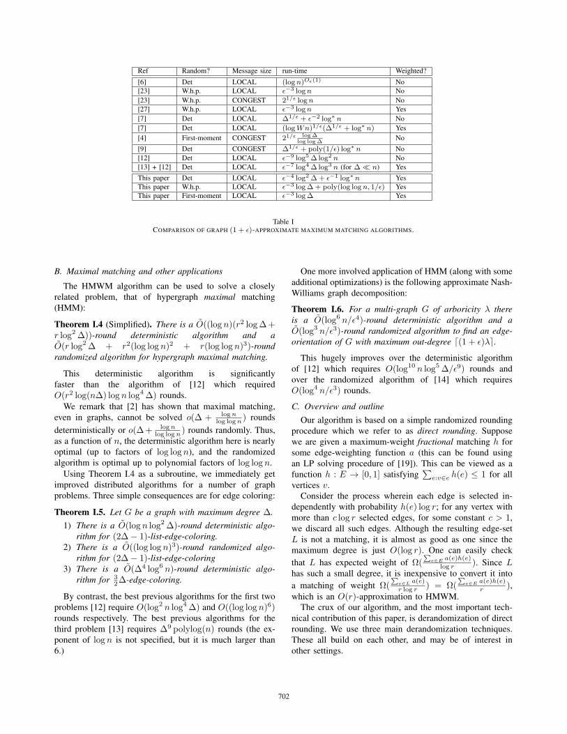
We summarize a number of (1 + ε)-approximation

GMWM algorithms in Table I on the following page, listed

roughly in order of publication. For readability, we have

simplified the run-time bounds, omitting some asymptotic

notations as well as dropping some second-order terms.

Our HMWM algorithms yields a (1 + ε)-approximation

algorithm for graph matching:

Theorem I.3. For ε > 0, there is a O(ε−4 log2 Δ +ε−1 log∗ n)-round deterministic algorithm to get a (1 + ε)-approximate GMWM.

For any δ ∈ (0, 1/2), there is O(ε−3 logΔ +ε−3 log log 1

δ + ε−2(log log 1δ )

2)-round randomized algo-rithm to get a (1+ ε)-approximate GMWM with probabilityat least 1− δ.

For a first-moment bound, we can take δ = ε getting

O(ε−3 logΔ) run-time. For success w.h.p., we can take

δ = 1/ poly(n) getting O(ε−3 logΔ + ε−3 log log n +ε−2(log logn)2) run-time.

Both the randomized and deterministic algorithms here

improve qualitatively over prior GMWM approximation

algorithms. These are the first (1 + ε)-approximation algo-

rithms (either randomized or deterministic) that simultane-

ously have three desirable properties: (1) run-time essentially

independent of n; (2) allowing arbitrary edge weights,

without any assumptions or run-time dependence on the

maximum edge weight W ; and (3) a polynomial dependence

on 1/ε.

Note that for any fixed ε, the deterministic algorithm has

a run-time which matches that of the fastest prior constant-factor approximation algorithms [1], [8], which are based on

using alternating paths to convert fractional matchings into

integral matchings.

For lower bounds, [19] shows that

Ω(min(√

lognlog logn ,

logΔlog logΔ )) rounds are needed for

any constant-factor approximation to GMWM, even for

randomized algorithms. Thus, these algorithm run-times are

close to optimal, and the randomized algorithm has optimal

run-time up to factors of log logΔ.

701

Ref Random? Message size run-time Weighted?

[6] Det LOCAL (logn)Oε(1) No

[23] W.h.p. LOCAL ε−3 logn No

[23] W.h.p. CONGEST 21/ε logn No

[27] W.h.p. LOCAL ε−3 logn Yes

[7] Det LOCAL Δ1/ε + ε−2 log∗ n No

[7] Det LOCAL (logWn)1/ε(Δ1/ε + log∗ n) Yes

[4] First-moment CONGEST 21/ε logΔlog logΔ

No

[9] Det CONGEST Δ1/ε + poly(1/ε) log∗ n No

[12] Det LOCAL ε−9 log5 Δ log2 n No

[13] + [12] Det LOCAL ε−7 log4 Δ log3 n (for Δ � n) Yes

This paper Det LOCAL ε−4 log2 Δ+ ε−1 log∗ n Yes

This paper W.h.p. LOCAL ε−3 logΔ + poly(log logn, 1/ε) Yes

This paper First-moment LOCAL ε−3 logΔ Yes

Table ICOMPARISON OF GRAPH (1 + ε)-APPROXIMATE MAXIMUM MATCHING ALGORITHMS.

B. Maximal matching and other applications

The HMWM algorithm can be used to solve a closely

related problem, that of hypergraph maximal matching

(HMM):

Theorem I.4 (Simplified). There is a O((log n)(r2 logΔ+r log2 Δ))-round deterministic algorithm and aO(r log2 Δ + r2(log logn)2 + r(log logn)3)-roundrandomized algorithm for hypergraph maximal matching.

This deterministic algorithm is significantly

faster than the algorithm of [12] which required

O(r2 log(nΔ) log n log4 Δ) rounds.

We remark that [2] has shown that maximal matching,

even in graphs, cannot be solved o(Δ + lognlog logn ) rounds

deterministically or o(Δ+ lognlog logn ) rounds randomly. Thus,

as a function of n, the deterministic algorithm here is nearly

optimal (up to factors of log logn), and the randomized

algorithm is optimal up to polynomial factors of log logn.

Using Theorem I.4 as a subroutine, we immediately get

improved distributed algorithms for a number of graph

problems. Three simple consequences are for edge coloring:

Theorem I.5. Let G be a graph with maximum degree Δ.1) There is a O(log n log2 Δ)-round deterministic algo-

rithm for (2Δ− 1)-list-edge-coloring.2) There is a O((log log n)3)-round randomized algo-

rithm for (2Δ− 1)-list-edge-coloring3) There is a O(Δ4 log6 n)-round deterministic algo-

rithm for 32Δ-edge-coloring.

By contrast, the best previous algorithms for the first two

problems [12] require O(log2 n log4 Δ) and O((log log n)6)rounds respectively. The best previous algorithms for the

third problem [13] requires Δ9 polylog(n) rounds (the ex-

ponent of log n is not specified, but it is much larger than

6.)

One more involved application of HMM (along with some

additional optimizations) is the following approximate Nash-

Williams graph decomposition:

Theorem I.6. For a multi-graph G of arboricity λ thereis a O(log6 n/ε4)-round deterministic algorithm and aO(log3 n/ε3)-round randomized algorithm to find an edge-orientation of G with maximum out-degree �(1 + ε)λ�.

This hugely improves over the deterministic algorithm

of [12] which requires O(log10 n log5 Δ/ε9) rounds and

over the randomized algorithm of [14] which requires

O(log4 n/ε3) rounds.

C. Overview and outline

Our algorithm is based on a simple randomized rounding

procedure which we refer to as direct rounding. Suppose

we are given a maximum-weight fractional matching h for

some edge-weighting function a (this can be found using

an LP solving procedure of [19]). This can be viewed as a

function h : E → [0, 1] satisfying∑

e:v∈e h(e) ≤ 1 for all

vertices v.

Consider the process wherein each edge is selected in-

dependently with probability h(e) log r; for any vertex with

more than c log r selected edges, for some constant c > 1,

we discard all such edges. Although the resulting edge-set

L is not a matching, it is almost as good as one since the

maximum degree is just O(log r). One can easily check

that L has expected weight of Ω(∑

e∈E a(e)h(e)

log r ). Since Lhas such a small degree, it is inexpensive to convert it into

a matching of weight Ω(∑

e∈L a(e)

r log r ) = Ω(∑

e∈E a(e)h(e)

r ),which is an O(r)-approximation to HMWM.

The crux of our algorithm, and the most important tech-

nical contribution of this paper, is derandomization of direct

rounding. We use three main derandomization techniques.

These all build on each other, and may be of interest in

other settings.

702

In Section II, we describe the first technique for deran-

domizing general LOCAL graph algorithms. This is an adap-

tation of [12] using the method of conditional expectations

via a proper vertex coloring. Roughly speaking, in each

stage i, all the vertices of color i select a value for their

random bits to ensure that the conditional expectation of

some statistic of interest does not decrease. The objective

function here acts in a black-box way and can be almost

completely arbitrary.

In Section III, we develop our second derandomization

technique, which extends this first method to allow a non-proper vertex coloring. This allows fewer colors, leading

to a faster run-time. This new algorithm is fundamentally

white-box: it requires the use of a carefully tailored pes-

simistic estimator for the conditional expectation. To state

it somewhat informally, the estimator must be “multilinear”

with respect to the coloring. This allows all the vertices of a

given color to simultaneously make their decisions without

non-linear interactions.

While this is a significant restriction, we also show that

such a pessimistic estimator comes naturally for Chernoff

bounds. To explain this at at a very high level, concentration

bounds with probabilities of order δ require bounds on the

joint behavior of w-tuples of vertices for w = O(log 1δ ). For

an appropriately chosen improper vertex coloring, most such

w-tuples will have vertices of different colors.

In Section IV, we turn this machinery to derandomize

direct rounding. To do so, we slow down the random process:

instead of selecting the edges with probability p = h(e) log rat once, we go through multiple stages in which each edge

is selected with probability 1/2. We then use the conditional

expecations method at each stage, ensuring that the weight

of the retained edges at the end is at least the expected

weight initially; we have seen this is Ω(∑

e a(e)h(e)

log r ). This is

the most technically complex part of the paper. The statistic

is a complex, non-linear function, so instead of directly

computing its conditional expectation, we carefully construct

a family of pessimistic estimators which approximate it but

are amenable to the derandomization method in Section III.

This algorithm runs in O(r logΔ + log2 Δ) rounds to

generate the O(r)-approximate maximum weight matching.

In particular this is scale-free, without dependence on n.

We find it somewhat remarkable that it is possible to

deterministically optimize a global statistic∑

e∈L a(e) in

an almost completely local way. (Although this part of the

algorithm is completely local, it still depends on finding an

appropriate proper vertex coloring, which requires O(log∗ n)rounds.)

In Section V, we describe how to perform the initial

step of obtaining the fractional matching. In addition to the

LP solving algorithm of [19], we employ a few additional

quantization steps. For the randomized algorithm, we also

randomly sparsify the original graph, reducing the degree

from Δ to log 1δ where δ is the desired failure probability,

and then we execute the deterministic algorithm. Note that

the deterministic algorithm is obtained by derandomizing

direct rounding, and the randomized algorithm is obtained

by “randomizing” the deterministic algorithm. The resulting

randomized algorithm, after these two transformations, has a

failure probability which is exponentially smaller than direct

rounding.

In Section VI, we use approximate HMWM to get a

(1+ε)-approximation to GMWM. As we have discussed, the

GMWM algorithm repeatedly finds and applies a collection

of disjoint high-weight augmenting paths. Our hypergraph

matching algorithm can be used for this step of finding the

paths. After multiple iterations of this process the resulting

graph matching is close to optimal. It is critical here that

our algorithm finds a high-weight hypergraph matching, not

merely a maximal matching. We also provide further details

on lower bounds for GMWM.

In Section VII, we discuss HMM, including an application

to edge-list-coloring. The basic algorithm for HMM is

simple: at each stage, we try to find a hypergraph matching

of maximum cardinality in the residual graph. Our HMWM

approximation algorithm ensures that the maximum match-

ing cardinality in the residual graph decreases by a 1− 1/rfactor in each stage. Thus we have a maximal matching after

O(r log n) repetitions. For the randomized algorithm, we

also take advantage of the “shattering method” of [3]. Our

algorithm here is quite different from a standard shattering-

method construction, so we provide a self-contained descrip-

tion in this paper.

In Section VIII, we describe a more elaborate application

of HMM to approximate Nash-Williams decomposition. We

describe both randomized and deterministic algorithms for

this task. Counter-intuitively, the deterministic algorithm is

built on our randomized HMM algorithm.

D. Comparison with related work

The basic framework of our algorithm, like that of [9],

[12], is to start with a fractional matching h, and then round

it to an integral one (at some loss to its weight). This can

be interpreted combinatorially as the following problem:

given a hypergraph H = (V,E), find a matching of weight

approximately∑

e∈E a(e)

Δr for some edge-weighting function

a. Let us summarize the basic approach taken by [9] and

[12] and how we are improve the complexity.

The algorithm of [9] gives an O(r3)-approximation to

HMWM in O(r2(logΔ)6+log r +log∗ n) rounds. It is based

on a primal-dual method: the fractional matching is gradu-

ally rounded, while at the same time a vertex cover (which

is the dual problem to maximum matching) is maintained to

witness its optimality.

The algorithm of [12], like ours, is based on derandom-

ized rounding. They only aim for a hypergraph maximal

matching, not an approximate HMWM. The key algorithmic

subroutine for this is degree-splitting: namely, selecting an

703

edge-set E′ ⊆ E which has degree at most Δ2 (1 + ε) and

which contains approximately half of the edges. This has

a trivial 0-round randomized algorithm, by selecting edges

independently with probability 1/2. To derandomize this,

[12] divides H into “virtual nodes” of degree lognε2 . They

then get a proper vertex coloring of the resulting line graph

(which has maximum degree r lognε2 ), and derandomize using

the method of conditional expectations.

To reduce the degree further, [12] repeats this edge-

splitting process for s ≈ log2 Δ steps. This generates nested

edge-sets E = E0 ⊇ E1 ⊇ · · · ⊇ Es wherein each Ei has

degree at most Δ( 1+ε2 )i and has |Ei| ≈ 2−i|E|. The final

set Es has very small maximum degree, and a much simpler

algorithm can then be used to select a large matching of it.

The process of generating nested edge sets E0, . . . , Es

with decreasing maximum degree is superficially quite

similar to our derandomization of direct rounding. Both

algorithms generate nested edge sets which simulate the

random process of retaining edges independently. But there

are two key differences between the methodologies.

First, and less importantly, the algorithm of [12] aims to

ensure that all the vertices have degree at most Δ2 (1 + ε).

Since they use a random process based on a union bound

over the vertices, this means they pay a factor of log n in

the run-time. Second, in order to use degree-splitting over sstages with only a constant-factor overall loss, the algorithm

of [12] needs (1 + ε)s = O(1), i.e., ε ≈ 1/ logΔ. This

is a very strict constraint: every vertex v must obey tight

concentration bounds at each of the stages i = 1, . . . , s.

These concentration bounds together give a complexity

of O(r log n/ε2) = O(r log n log2 Δ) per stage, and total

complexity of O(r log n log3 Δ) over all stages.

Let us discuss how our algorithm avoids these issues. Like

the algorithm of [9], we aim for a run-time independent

of n. To this end, we do not insist that all vertices have

their degree reduced. We discard the vertices for which

certain bad-events occur, e.g. the degree is much larger than

expected. These are rare so this does not lose too much in

the weight of the matching.

Second, we observe that, if we actually ran the multi-stage

process randomly, it would not be unusual for the degree of

any given vertex v to deviate significantly from its mean

value in a single stage. It would be quite rare to have such a

deviation in all s stages. Thus, we really need to keep track

of the total deviation of deg(v) from its mean value across

all the stages, aggregated over all vertices v. This is precisely

what we achive through our potential function analysis of

direct rounding. By allowing more leeway for each vertex

per stage, we can get away with looser concentration bounds,

and correspondingly lower complexity.

E. Notation and conventions

For a graph G = (V,E) and v ∈ V , we define N [v] to

be the inclusive neighborhood of vertex v, i.e. {v} ∪ {w |

(w, v) ∈ E}. For a hypergraph H = (V,E) and v ∈ V ,

we define N(v) to be the set of edges e � v. We define

deg(v) = |N(v)| and for L ⊆ E we define degL(v) =|N(v) ∩ L|. Unless stated otherwise, E may be a multi-set.

For a set X and integer k, we define(Xk

)to be the set

of all k-element subsets of X , i.e. the collections of sets

Y ⊆ X, |Y | = k.

For a graph G = (V,E), we define the power graph Gt

to be a graph with vertex set V , and with an edge (u, v) if

there is a path of length up to t in G. Note that if G has

maximum degree Δ, then Gt has maximum degree Δt.

We define a fractional matching to be a function h : E →[0, 1] such that

∑e∈N(v) h(e) ≤ 1 for every v ∈ V . Note

that this should be distinguished from a fractional solution

to the matching polytope of a graph, which also includes

constraints for all odd cuts.

For any edge-weighting function a : E → [0,∞), and

any edge subset L ⊆ E, we define a(L) =∑

e∈L a(e).Similarly, for a fractional matching, we define a(h) =∑

e∈E h(e)a(e). Finally, for any hypergraph H = (V,E)we write a(H) as shorthand for a(E).

For any function a : E → [0,∞) we define a∗ to be the

maximum-weight fractional matching with respect to edge-

weight function a.

For any boolean predicate P , we use the Iverson notation

so that [[P]] is the indicator function that P is true, i.e.

[[P]] = 1 if P is true and [[P]] = 0 otherwise.

We use the O() notation throughout, where we define

O(x) to be x polylog(x).

F. The LOCAL model for hypergraphs

Our algorithms are all based on the LOCAL model for

distributed computations in a hypergraph. This is a close

relative to Linial’s classic LOCAL graph model [21], [29],

and in fact the main motivation for studying hypergraph

LOCAL algorithms is because they are useful subroutines

for LOCAL graph algorithms. Let us first describe how the

LOCAL model works for graphs.

There are two variants of the LOCAL model involving

randomized or deterministic computations. In the determin-

istic variant, each vertex is provided with a unique ID which

is a bitstring of length Θ(log n); here the network size n is a

global parameter passed to the algorithm. A vertex has a list

of the ID’s of its neighbors. Time proceeds synchronously: in

any round a vertex can perform arbitrary computations and

transmit messages of arbitrary sizes to its neighbors. At the

end of this process, each vertex must make some decision

as to some local graph problem. For example, if the graph

problem is to compute a maximal independent set, then each

vertex v sets a flag Fv indicating whether it has joined the

MIS.

The closely related randomized model has each vertex

maintain a private random string Rv of unlimited length. As

before, time proceeds synchronously and all steps except the

704

generation of Rv can be regarded as deterministic. At the

end of the process, we only require that the flags Fv correctly

solve the graph problem w.h.p., i.e. with probability at least

1− n−c for any desired constant c > 0.

To define the LOCAL model on a hypergraph H , we first

form the incidence graph G = Inc(H); this is a bipartite

graph in which each edge and vertex of H corresponds to a

vertex of G. If uv and ue are the vertices in G corresponding

to the vertex v ∈ V and e ∈ E, then G has an edge (ue, uv)whenever v ∈ e. The LOCAL model for hypergraph H is

simply the LOCAL graph model on G. In other words, in a

single timestep on the hypergraph H , each vertex can send

arbitrary messages to every edge e ∈ N(v), and vice versa.

The connection between the hypergraph and graph LO-

CAL model goes both ways. For a number of LOCAL graph

algorithms, we need structures such as maximal disjoint

paths. The length-� paths of a graph G can be represented as

hyperedges in an auxiliary hypergraph H of rank �. Further-

more, a communication step of H can be simulated in O(�)rounds of the communication graph G. Most applications of

HMM come from this use a subroutine for graph algorithms.

Many graph and hypergraph algorithms depend on the

maximum degree Δ, rank r, and vertex count n. These pa-

rameters cannot actually be computed locally. As is standard

in distributed algorithms, we consider Δ, r, n to be globally-

known upper-bound parameters which are guaranteed to

have the property that |N(v)| ≤ Δ, |e| ≤ r, |V | ≤ n for

every vertex v and edge e. When V is understood, we may

say that E has maximum degree Δ and maximum rank r.

We also assume throughout that r ≥ 2, as the cases r = 0and r = 1 are trivial. In many cases where hypergraph

matching is used as a subroutine, we can deduce such upper

bounds from the original, underlying graph problem. (In

certain cases, LOCAL algorithms can be used without a

priori bounds on Δ, r, n (see, for example [18]), but for

simplicity we do not explore this here.)

In the case of weighted matchings, we let W denote the

ratio between maximum and minimum edge weight. We

note that our algorithm does not require that W is globally

known, or is bounded in any way; the algorithm behavior is

completely oblivious to this parameter.

II. DERANDOMIZATION VIA PROPER VERTEX COLORING

To begin our derandomization analysis, we describe a gen-

eral method of converting randomized LOCAL algorithms

into deterministic ones via proper vertex coloring. This is

a slight variant of the method of [12] based on conditional

expectations; we describe it here to set the notation and since

some of the parameters are slightly different.

Consider a 1-round randomized graph algorithm A run on

a graph G = (V,E); at the end of this process, each vertex

v has a real-valued flag Fv . In this randomized process, we

let Rv denote the random bit-string chosen by vertex v; to

simplify the analysis, we take Rv to be an integer selected

uniformly from the range {0, . . . , γ − 1} for some finite

value γ. We define �R to be the overall collection of values

Rv , and we also define R = {0, . . . , γ − 1}n to be the

space of all possible values for �R. In this setting, each Fv

can be considered as a function mapping R to R. Since

the algorithm A takes just 1 round, each value Fv(�R) is

determined by the values Rw for w ∈ N [v]. (The extension

to multi-round LOCAL algorithms will be immediate.)

Lemma II.1. Suppose that G2 has maximum degree d. Thenthere is a deterministic graph algorithm in O(d + log∗ n)rounds to determine values �ρ for the random bits �R, suchthat when (deterministically) running A with the values �R =�ρ, it satisfies ∑

v

Fv(�ρ) ≤ E[∑v

Fv(�R)]

Furthermore, when given a O(d) coloring of G2 as input,the additive factor of log∗ n can be omitted.

Proof: We set the bits Rv using the method of condi-

tional expectations. See [12] for a full exposition; we provide

just a sketch here.

If we are not already given a proper vertex coloring

of G2 with O(d) colors, we use the algorithm of [10] to

obtain this in O(√d)+O(log∗ n) rounds. Next, we proceed

sequentially through the color classes; at the ith stage, every

vertex v of color i selects a value ρv to ensure that the

expectation of Fv +∑

(u,v)∈E Fu, conditioned on Rv = ρv ,

does not increase. Note that all the vertices of color i are

non-neighbors, so they do not interfere during this process.

This setting, wherein the statistic of interest is∑

v Fv , is

more general than the setting of locally-checkable problems

considered in [12]. The flag Fv here is not necessarily

interpreted as an indication that the overall algorithm has

failed with respect to v, and indeed it may not be possible

for any individual vertex v to witness that the algorithm has

failed.

Also, Lemma II.1 is stated in terms of minimizing the

sum∑

v Fv(�ρ); by replacing F with −F , we can also

maximize the sum, i.e. get∑

v Fv(�ρ) ≥ E[∑

v Fv(�R)]. In

our applications, we will use whichever form (maximization

or minimization) is most convenient; we do not explicitly

convert between these two forms by negating the objective

functions.

To derandomize hypergraph LOCAL algorithms, we apply

Lemma II.1 to the incidence graph G = Inc(H). It is

convenient to rephrase Lemma II.1 in terms of H without

explicit reference to G.

Definition II.2. For a hypergraph H of rank r and maximumdegree Δ, and incidence graph G, we define a good coloring

of H to be a proper vertex coloring of G2 with O(rΔ)colors.

705

Lemma II.3. Let A be a randomized 1-round algorithm runon a hypergraph H = (V,E) of rank r and maximum degreeΔ. Each u ∈ V ∪ E has private random bitstring Ru andat the termination of A it outputs the real-valued quantitiesFu. If we are provided a good coloring of H , then there is adeterministic O(rΔ)-round algorithm to determine values �ρsuch that when (deterministically) running A with the values�R = �ρ, it satisfies∑

u∈V ∪EFu(�ρ) ≤ E[

∑u∈V ∪E

Fu(�R)]

Proof: Let G be the incidence graph of H . Note that

G2 has maximum degree d = Δr. A good coloring of H is

by definition a O(d) coloring of G2. Now apply Lemma II.1

with respect to G.

As a simple application of Lemma II.3, which we need

later in our algorithm, we consider a straightforward round-

ing algorithm for matchings.

Lemma II.4. Let H = (V,E) be a hypergraph with anedge-weighting a : E → [0,∞) and a good coloring ofH . Then there is a deterministic O(rΔ)-round algorithm tocompute a matching M with a(M) ≥ Ω(a(E)

rΔ ).

Proof: We provide a sketch here; the full proof is in

Appendix A. Consider the following 1-round randomized

algorithm: we generate edge-set L ⊆ E, wherein each edge

e ∈ E goes into L independently with probability p = 0.1rΔ .

Next, we form a matching M from L by discarding any pair

of intersecting edges. Let us define the following statistic on

L:

Φ(L) :=∑e∈E

a(e)[[e ∈ L]]−∑v∈V

∑e,e′∈N(v)

e′ �=e

a(e)[[e ∈ L∧e′ ∈ L]]

One can easily see that a(M) ≥ Φ(L) and that E[Φ(L)] ≥Ω(a(E)

rΔ ). Furthermore, the statistic Φ(L) has the required

form for Lemma II.3, where the flag Fu for u ∈ V ∪ E is

defined as

Fe = [[e ∈ L]]a(e),

Fv =∑

e,e′∈N(v)e�=e′

−[[e ∈ L ∧ e′ ∈ L]]a(e)

Lemma II.3 thus gives an edge-set L with Φ(L) ≥E[Φ(L)]. The resulting matching M satisfies a(M) ≥Ω(a(E)

rΔ ) as desired.

The method of derandomization via proper vertex coloring

is not satisfactory on its own, because of its polynomial

dependence on Δ. We remove this by adapting the degree-

splitting algorithm of [12]. The following definitions are

useful to characterize this process:

Definition II.5 (frugal and balanced edge colorings). For ahypergraph H and edge-coloring χ : E → {1, . . . , k}, we

say that the coloring χ is t-frugal if every vertex v has atmost t edges of any given color j; more formally, if |N(v)∩χ−1(j)| ≤ t for all v ∈ V, j ∈ {1, . . . , k}.

We say that an edge-coloring χ : E → {1, . . . , k} isbalanced if it is t-frugal for t = O(Δ/k).

Note that a proper edge coloring would typically not be

balanced, as it would have frugality t = 1 and use k = rΔcolors. The trivial randomized coloring algorithm gives a

balanced edge coloring for t = log n. The main contribution

of [12] is to derandomize this, getting a balanced coloring

with t = polylog n. This dependence on n is not suitable

for us; we want t to depend only on local parameters r,Δ.

A simple application of the iterated Lovasz Local Lemma

(LLL) shows that a balanced edge-coloring exists for t =log r. Unfortunately, even the randomized LLL algorithms

are too slow for us. We will settle for something slightly

weaker: we get a partial frugal edge-coloring. This can be

obtained by iterating the following simple 1-round random-

ized algorithm: first randomly 2-color the edges, and then

discard all edges incident to a vertex with more than Δ2 (1+ε)

edges of a color. This serves as a “poor man’s LLL”.

We summarize our edge coloring result as follows. The

proof is similar to the work [12], so we defer it to Ap-

pendix A.

Lemma II.6. Suppose we are given a good coloring ofhypergraph H = (V,E) with rank r and maximum degreeΔ. For any δ ∈ (0, 1) and integer parameter k ≥ 2 satisfyingΔ ≥ Ck2 log r

δ for some absolute constant C, there is anO(r log 1

δ log3 k)-round deterministic algorithm to find an

edge set E′ ⊆ E with an edge-coloring χ : E′ → {1, . . . , k}such that

1) a(E′) ≥ (1− δ)a(E)2) χ is t-frugal on E′ for parameter t = 4Δ/k.

In particular the coloring χ is balanced.

A remark on maintaining good colorings. A typical

strategy for our algorithms will be to first get a poly(r,Δ)coloring of the original input hypergraph H , in O(log∗ n)rounds, using the algorithm of [22]. Whenever we modify H(by splitting vertices, replicating edges, etc.) we will update

the coloring. All these subsequent updates can be performed

in O(log∗(rΔ)) rounds [22]. Whenever we need an O(rΔ′)coloring of some transformed hypergraph H ′, we use the

algorithm of [10] to obtain it in o(rΔ′) + O(log∗(rΔ))rounds. These steps are all negligible compared to the

runtime of the overall algorithm.

These coloring updates are routine but quite cumbersome

to describe. For simplicity of exposition, we will mostly

ignore them for the remainder of the paper.

706

III. DERANDOMIZATION WITHOUT PROPER VERTEX

COLORING

The use of a proper vertex coloring χ in the proof

of Lemma II.1 is somewhat limiting. In this section, we

describe how to relax this condition. To make this work, we

require that the statistic Φ =∑

u Fu we are optimizing is

highly tailored to χ; this is quite different from Lemma II.1,

in which the function Fu is almost arbitrary and is treated

in a black-box way. The derandomization result we get this

way may seem very abstract. We follow with an example

showing how it applies to concentration bounds for sums of

random variables.

Let us briefly explain the intuition. If χ is a non-proper

vertex coloring and we try to use the conditional expectation

method of Lemma II.1, we will incorrectly compute the

contributions from adjacent vertices of the same color. The

reason for this is that the randomness for one may interact

with the randomness for the other one. To avoid these errors,

we carefully construct the statistic Φ to be “multilinear”

with respect to the coloring χ. This avoids the problematic

non-linear interactions. (Linear interactions do not cause

problems.)

Let us note that a similar type of derandomization strategy

using a non-proper vertex coloring is used in [17]. These

methods are somewhat similar, but the work of [17] is

based on ignoring all interactions between vertices with the

same color, followed by a postprocessing step to correct the

resulting errors. There is a key difference in our approach to

the error term. Our statistic Φ is an approximation to the true

statistic of interest (incurring some error), but the algorithm

still “correctly” handles the linear interactions and incurs no

further error in derandomizing it.

A. The derandomization lemma

Consider some graph G = (V,E) with some global

statistic Φ : R→ R which is a function of the random bits.

Each vertex may have some additional, locally-held state; for

example, we may be in the middle of a larger multi-round

algorithm and so each node will have seen some information

about its t-hop neighborhood. The function Φ may depend

on this vertex state as well; to avoid burdening the notation,

we do not explicitly write the dependence.

We need the statistic Φ to obey a certain multilinearity

condition, i.e. it has no mixed derivatives of a certain kind. In

order to define, we need to analyze the directional derivative

structure of Φ.

In the applications in this paper, we will only need to

analyze a relatively simple probabilistic process, wherein

every vertex chooses a single bit uniformly at random. In the

language of Section II, this is the setting with γ = 2. In order

to simplify the definitions and exposition here, we will focus

solely on this case; the results can easily be generalized to

more complicated probability distributions.

Thus, we view Φ as a function mapping {0, 1}V to R.

Formally, for any vertex v ∈ V we define the derivativeDvΦ as follows:

(DvΦ)(x1, . . . , xn) = Φ(x1, . . . , xv−1, xv, xv+1, . . . , xn)

− Φ(x1, . . . , xv−1, xv, xv+1, . . . , xn)

where here xv denotes flipping the value of bit xv . Note that

DvΦ is itself a function mapping R to R, so we can talk

about its derivatives as well.

Definition III.1 (uncorrelated potential function). FunctionΦ is pairwise uncorrelated for vertices v, v′ if the functionDvDv′Φ is identically zero. We say that Φ is uncorrelated

for vertices v1, . . . , vs if it is pairwise uncorrelated for everypair vi, vj and i �= j.

We are now ready to state our main derandomization

lemma.

Lemma III.2. Suppose that we are provided a vertexcoloring χ : V → {1, . . . , k} (not necessarily proper) for G,where the potential function Φ : R → R has the followingproperties:(A1) For all vertices v, w with (v, w) /∈ E, the function Φ

is pairwise uncorrelated for v, w.(A2) For all vertices v, w with v �= w and χ(v) = χ(w),

the function Φ is pairwise uncorrelated for v, w.(A3) For any vertex v, the value of DvΦ(x1, . . . , xn) can

be locally computed by v given the values of xw forw ∈ N [v].

Then there is a deterministic O(k)-round algorithm todetermine values �ρ for the random bits, such that Φ(�ρ) ≤E[Φ(�R)].

Proof: We provide a sketch here; see Appendix A for

further details.

We proceed through stages i = 1, . . . , k; at each stage

i, every vertex v with χ(v) = i selects some value ρv so

that E[DvΦ | Rv = ρv] ≥ 0, and permanently commits to

Rv = ρv .

We first claim that this information can be computed

by v in O(1) rounds. By Property (A1), the conditional

expectation E[DvΦ | Rv = x] only depends on the values

of Rw for w ∈ N(v). Thus in O(1) rounds v can query the

values of ρw for w ∈ N(v). It can then integrate over the

possible random values for all Rw in its neighborhood and

use Property (A3) to determine E[DvΦ | Rv = x] for all

values x and u. This allows it to determine ρv .

Finally, Property (A2) ensures that the decision made for

each vertex v does not interfere with any other vertex v′ of

the same color. Therefore, the conditional expectation of Φdoes not increase during the round i.

Lemma II.1 is a special case of Lemma III.2: for, consider

a 1-round LOCAL algorithm which computes for each

vertex v a function Fv . If χ is a proper vertex coloring

707

of G2, then the potential function Φ =∑

v∈V Fv satisfies

Lemma III.2 with respect to the graph G2. (Condition (A2)

is vacuous, as vertices v, w with χ(v) = χ(w) must be non-

neighbors and hence by (A1) they are pairwise uncorrelated.)

B. Example: derandomizing edge-splitting

For better motivation, we consider a simplified example,

in which Φ corresponds to Chernoff-type bounds on the

deviations of sums of random variables. There is a par-

ticularly powerful and natural way to apply Lemma III.2

in this setting. (In our application later in Section IV, we

will encounter something similar to this, but much more

complex.) To provide more intuition, we will not carry out

any detailed error estimates.

Let us consider a Δ-regular hypergraph H = (V,E) (i.e.

every vertex v has deg(v) = Δ) and consider the random

process where each edge e ∈ E is added to a set L with

probability 1/2. Our statistic of interest is

Φ(L) =∑v

a(v)[[| degL(v)− Δ

2 | ≥ t]]

for some function a : V → R and some desired parameter

t. We would like to select some (deterministic) edge set Lsuch that

Φ(L) ≤ E[Φ] =∑v

a(v) Pr(| degL(v)− Δ

2 | ≥ t)

We are going to apply Lemma III.2 to the graph G =Inc(H)2. We actually only care about the nodes of G cor-

responding to edges of H; the nodes of G corresponding to

vertices are immaterial and will be ignored. Thus, the vertex-

coloring of G that will be used for Lemma III.2 corresponds

to an edge-coloring of H . Note that all the results and

terminology in Lemma III.2 regarding vertex colors should

be translated into edge colors for this application.

Accordingly, let us first choose a balanced k-edge coloring

χ : E → {1, . . . , k} for k chosen appropriately. The choice

of k and the role played by χ will become clear shortly. Next

let us define the indicator variables Xe = [[e ∈ L]], which

are independent Bernoulli-1/2 random variables. At this

point, we use a result of [31] based on a connection between

Chernoff bounds and symmetric polynomials, which is based

on the following inequality:

[[degL(v) ≥ μ(1 + δ)]] ≤(degL(v)

w

)(μ(1+δ)

w

)=

∑W∈(N(v)

w )∏

e∈W Xe(μw

)for any integer w ≤ μ(1 + δ), where μ = Δ

2 and δ = t/μ.

This bound is powerful because we can then calculate

Pr(degL(v) ≥ μ(1 + δ)) ≤∑

W∈(N(v)w ) E[

∏e∈W Xe](

μ(1+δ)w

) ;

further calculations of [31] show that for w = �t� the

RHS is at most the well-known Chernoff bound ( eδ

(1+δ)1+δ )μ.

Smaller values of w also yield powerful concentration

bounds, with probability bounds roughly inverse exponential

in w.

The denominator here is a constant for all v, so it can be

ignored. Thus, as a proxy for Φ(L), it would be natural to

use a pessimistic estimator

Φ′(L) =∑v

a(v)∑

W∈(N(v)w )

( ∏e∈W

Xe +∏e∈W

(1−Xe))

Unfortunately, this function Φ′ is not compatible with

Lemma III.2. The problem is that some set W ⊆ N(v)may contain multiple edges with the same color; for a

pair of edges e1, e2 ∈ N(v), a term such as∏

e∈W Xe +∏e∈W (1−Xe) will have a non-vanishing second derivative

De1De2

∏e∈W Xe.

To avoid this, we need another statistic Φ′′. For any vertex

v, define Uv to be the set of all subsets W ∈ (N(v)w

)such

that all edges f in W have distinct colors. If we restrict the

sum to only the subsets W ∈ Uv , then we get a statistic

which is compatible with Lemma III.2:

Φ′′(L) =∑v

a(v)∑

W∈Uv

( ∏e∈W

Xe +∏e∈W

(1−Xe))

To show that this satisfies (A1), note that if e1 and e2are not connected in G2, then at most one of them involves

vertex v. Thus, the set W contains at most one of the edges

e1, e2 and so De1De2

∏e∈W Xe = 0.

To show property (A2), suppose that χ(e1) = χ(e2). Then

any W ∈ Uv contains at most one of e1, e2, and so the

second derivative De1De2(∏

e∈W Xe +∏

e∈W (1 − Xe) is

indeed zero.

To show that this satisfies (A3), we compute the first

derivative De1 as:

De1Φ′ =

∑v

a(v)∑

W∈Uv :e1∈WDe1

( ∏e∈W

Xe+∏e∈W

(1−Xe))

For such W , all the other edges e ∈W also involve vertex

v, and so e is a neighbor to e1 in G2. So all such terms can

be computed locally by e1.

This means that Lemma III.2 applies to Φ′′, and we get

a subset L with Φ′′(L) ≥ E[Φ′′(L)]. But this is not what

we want; we want Φ(L) ≥ E[Φ(L)]. This is where our

derandomization incurs some small error.

We will not bound the error rigorously here. But, at a

high level, let us explain why it should be small. Consider

some randomly chosen subset W ⊆ N(v) of size w.

Since χ is b-frugal for b = O(Δ/k), the expected number

of pairs f1, f2 ∈ W with χ(f1) = χ(f2) is at most

w2b/Δ = O(w2/k). As long as k � w2, then, we expect

the edges in W have different colors, and hence W ∈ Uv,e.

708

Thus, most of the sets W ∈ (N(v)w

)are already in Uv,e. As

a result, we will have∑W∈Uv

∏e∈W

Xe ≈∑

W∈(N(v)w )

∏e∈W

Xe

and similarly for the terms∏(1−Xe).

For this reason, Φ′′(L) is quite close to Φ(L), and we

thus ensure that

Φ(L) ≈ Φ′′(L) ≥ E[Φ′′(L)] ≈ E[Φ(L)]

which is (up to some small error terms) precisely the

derandomization we want.

This example illustrates three important caveats in using

Lemma III.2. First, we may have some natural statistic to

optimize in our randomized algorithm (e.g. the total weight

of edges retained in a coloring, indicator functions for

whether a bad-event has occurred). This statistic typically

will not satisfy condition (A2) directly. Instead, we must

carefully construct a pessimistic estimator which does satisfy

condition (A2).

Second, to avoid non-linear interactions, we must allow

some small error in our potential function. The potential

function must be carefully constructed so that these errors

remain controlled.

Finally, in order to apply Lemma III.2, we need an

appropriate coloring. In our hypergraph matching application

this will be a balanced frugal edge coloring χ. We first

obtain this coloring using the derandomization Lemma II.6.

We then craft the statistic for Lemma III.2 in terms of

χ Thus, each application of Lemma III.2 is essentially a

derandomization within a derandomization: we first use a

relatively crude method to obtain the needed coloring, and

then use this to obtain a more refined bound via Lemma III.2.

IV. DERANDOMIZATION OF DIRECT ROUNDING

We now use our derandomization methods to convert

a fractional matching into an integral one. We show the

following result:

Theorem IV.1. Let H = (V,E) be a hypergraph of max-imum degree Δ and rank r, along with an edge-weightingfunction a : E → [0,∞), and a good coloring of H . Thereis a O(log2 Δ + r logΔ)-round deterministic algorithm tofind a matching M with

a(M) ≥ Ω

(a(E)

rΔ

)

This value of a(M) is precisely what we would obtain

by applying Lemma II.4 to H . Unfortunately, Lemma II.4

would take O(rΔ) rounds, which is much too large.

So we need to reduce the degree of H . Consider the

following random process: we select each edge e ∈ Eindependently with probability p = Θ( log r

Δ ). If any vertex

v has degree larger than c log r for some constant c, we

discard all the selected edges. We let J denote the selected

edges and let J ′ ⊆ J denote the set of edges which are not

discarded.

Clearly, the hypergraph (V, J ′) has maximum degree

O(log r). It is not hard to see that E[a(J′)

log r ] ≥ Ω(a(E)Δ ).

(See Proposition A.5 for further details). We derandomize

this to geta(J ′)log r ≥ Ω(a(E)

Δ ) (in actuality, not expectation).

We can then follow up by applying Lemma II.4 to (V, J ′),obtaining a matching M with a(M) ≥ Ω(a(J

′)log r ) ≥ Ω(a(E)

Δ )

in O(r) rounds.

To derandomize this process, we first slow down the

randomness. Instead of selecting edge-set J in a single

stage, we go through log2(1/p) stages, in which each

edge is retained with probability 1/2. We use the method

of conditional expectations to select a series of edge-sets

E1, . . . , Es. Ideally, we would choose Ei = L such that

E[a(J ′) | Ei = L] ≥ E[a(J ′)]. In this conditional expecta-

tion, every edge e remaining in Ei will get selected for Jindependently with probability 2ip.

Unfortunately, the conditional expectation E[a(J ′) | Ei =L] is a complex, non-linear function of L, so we cannot

directly select L to optimize it. Instead, we carefully con-

struct a family of pessimistic estimator S0, . . . , Ss, which

are amenable to our derandomization Lemma III.2 and also

satisfies E[a(L′) | Ei = L] ≈ Si(L).For the remainder of this section, we assume that we

are given a good coloring of H and edge-weight function

a; these will not be mentioned specifically again in our

hypotheses.

A. The formal construction

For an edge-set L ⊆ E and integer i ∈ {0, . . . , s} we

define the potential function

Si(L) = ( 12α )

s−ia(L)

− bi∑v∈V

((Δ2−i

w

)+

(degL(v)

w

))a(N(v) ∩ L)

where we define the parameters as follows:

w = �2 log2(32r2 log2 Δ)�x = w4 log10(rΔ)

s = �log2 Δx �

α = 21/s

β = 16r(2x/w)w

bi = 2−(s−i)(w+1)αs−i/β

Our plan is to successively select edge subsets E = E0 ⊇E1 ⊇ · · · ⊇ Es, such that S0(E0) ≤ S1(E1) ≤ · · · ≤Ss(Es). Let us try to provide some high-level intuition for

the different terms in this expression. Here, the probability of

selecting an edge in the direct rounding would be p = 2−s ≈xΔ . We will form J ′ by discarding vertices with degree larger

than cx for some constant c. At stage i, the quantity Si(Ei)

709

is supposed to represent the expectation of a(J ′) after s− iadditional stages

The first term represents the expected weight of the

edges remaining in J , wjhich is a(Ei)2−(s+i). We include

an additional error term ( 1α )

s−i here, because some edges

will need to be discarded when we obtain our frugal edge

colorings.

The second term is supposed to represent the total weight

of the edges discarded due to vertices with excessive degree.

For a given vertex v and L = Ei, this expression is (up to

scaling factors) given by:

αs−i×2−(s−i)w((

Δ2−i

w

)+(degEi

(v)w

))×2−(s−i)a(N(v)∩Ei)

Let us see where these terms come from:

• The term αs−i is an additional fudge factor, accounting

for some small multiplicative errors in our approxima-

tions.

• The term 2−(s−i)a(N(v) ∩ Ei) is the expected value

of a(N(v) ∩ J)• The quantity 2−(s−i)w

(degEi

(v)w

)is roughly the ex-

pected value of(degJ (v)

w

), and thus (up to rescaling) an

approximation to the probability that that degJ(v)� x.

• Finally, let us explain the term(Δ2−i

w

). We only are

worried about vertices whose degree is much higher

than the expected value Δ2−i. If degEi(v) � Δ2−i,

then the term(degEi

(v)w

)will negligible compared to(

Δ2−i

w

)and so we can essentially ignore the vertex v.

We note that a similar technique of developing a pes-

simistic estimator for a polynomial potential function, and

derandomizing it via multiple rounds of conditional expecta-

tions was used in the algorithm of [15] for hypergraph MIS.

In particular, they developed the technical tool of using an

additive term to “smooth” errors in the multiplicative terms

of concentration inequalities, which we adopt here.

The key technical result for the algorithm will be the

following:

Lemma IV.2. Suppose Δ ≥ Δ0 for some universal constantΔ0. Given an edge-set L ⊆ E, there is a deterministic O(r+logΔ)-round algorithm to find an edge set L′ ⊆ L such thatSi+1(L

′) ≥ Si(L) and L′ has maximum degree Δ24−i.

This lemma is quite technically involved, and the proof

will involve a number of subclaims. We show it next in

Section IV-B. Before we do so, let us show some straightfor-

ward properties of the potential function, and also show how

Theorem IV.1 follows from the lemma. At several places, we

will use the elementary inequalities

pw(Tw

) ≥ (pTw

) ∀p ∈ [0, 1], T ∈ Z+ (1)

andx

4Δ≤ 2−s ≤ x

2Δ(2)

Proposition IV.3. We have S0(E) ≥ Ω(a(E)xΔ ).

Proof: As αs = 2 and using the inequality Eq. (2), at

i = 0 we have

( 12α )

s−ia(E) ≥ 2−s−1a(E) ≥ a(E)x

4ΔNext, let us consider some vertex v, and we

want to estimate the contribution of the term

bi((Δ2−i

w

)+

(degE(v)

w

))a(N(v) ∩ E). First, note that

b0 = 2−s(w+1)αs/β ≤ 1β × ( x

2Δ )w+1 × 2. By definition of

Δ, we have(degE(v)

w

) ≤ (Δw

). So

bi((Δ2−i

w

)+

(degE(v)

w

)) ≤ 2

β (x2Δ )w+1(

(Δw

)+

(Δw

))

= 4β (

x2Δ )w+1

(Δw

)≤ 4

β (x2Δ )w+1( eΔw )w

using the inequality(AB

) ≤ ( eAB )B

=4x

2βΔ× (

ex

2w)w ≤ 2x

βΔ(2x/w)w

Substituting in these values, we get

bi∑v∈V

((Δ2−i

w

)+

(degE(v)

w

))a(N(v) ∩ E)

≤ 2x

βΔ(2x/w)w

∑v∈V

a(N(v) ∩ E)

≤ 2rx(2x/w)w

βΔa(E) since H has rank at most r

=x

8Δsubstituting the value of parameter β

Thus S0(E) ≥ a(E)xΔ ( 14 − 1

8 ) ≥ Ω(a(E)xΔ ).

Proposition IV.4. Given a hypergraph H = (V,E) ofmaximum degree Δ with a good coloring, there is aO(r logΔ+log2 Δ)-round deterministic algorithm to find asubset E′ ⊆ E such that H ′ = (V,E′) has maximum degreeΔ′ ≤ polylog(Δ, r) and such that a(E′)/Δ′ ≥ Ω(a(E)/Δ)

Proof: We may assume that Δ is larger than any needed

constant, as otherwise taking E′ = E,Δ′ = Δ works.

Let E0 = E; we will proceed through s applications of

Lemma IV.2. At the ith stage, we apply Lemma IV.2 to Ei−1

to generate subset Ei ⊆ Ei−1 with Si(Ei) ≥ Si−1(Ei−1).We return the final set E′ = Es. Each such application

uses O(r + logΔ) rounds. There are s = O(logΔ) rounds

altogether, giving the stated complexity.In the initial hypergraph, Proposition IV.3 shows that

S0(E0) = S0(E) ≥ Ω(a(E)x/Δ). Because of the guarantee

of Lemma IV.2, we have Ss(Es) ≥ Ss−1(Es−1) ≥ · · · ≥S0(E0). Finally, let us observe that

Ss(Es) = a(Es)− bs∑v∈V

((Δ2−s

w

)+

(degEs

(v)w

))a(N(v) ∩ Es)

≤ a(Es).

Putting these inequalities together, we therefore have

a(Es) ≥ Ω(a(E)x

Δ)

710

On the other hand, Lemma IV.2 ensures that each Ei has

maximum degree Δ24−i, and in particular Es has maximum

degree Δ′ = Δ24−s = O(x) = polylog(Δ, r). Furthermore,

we have

a(Es)

Δ′≥ Ω(a(E)x/Δ)

O(x)≥ Ω(

a(E)

Δ)

To prove Theorem IV.1, we reduce the degree of H from

Δ to polyloglog(Δ) by two applications of Proposition IV.4.

Proof of Theorem IV.1: Given the initial hypergraph

H = (V,E) of maximum degree Δ, we apply Proposi-

tion IV.4 to obtain hypergraph H ′ = (V,E′) of maximum

degree Δ′ = polylog(r,Δ) and such that a(E′)/Δ′ ≥Ω(a(E)/Δ). Next, apply Proposition IV.4 to hypergraph H ′,obtaining a hypergraph H ′′ = (V,E′′) of maximum degree

Δ′′ = polylog(r,Δ′) = poly(log r, log logΔ) and such that

a(E′′)/Δ′′ ≥ Ω(a(E′)/Δ′) ≥ Ω(a(E)/Δ).

Finally, apply Proposition II.4 to hypergraph H ′′, obtain-

ing a matching M ⊆ E′′ such that a(M) ≥ Ω(a(E′′)

rΔ′′ ) ≥Ω(a(E)

rΔ ).

The first application of Proposition IV.4 takes O(log2 Δ+r logΔ) rounds. The second application takes O(log2 Δ′ +r logΔ′) rounds. The final application of Proposi-

tion II.4 takes O(rΔ′′) rounds. Noting that Δ′′ =poly(log r, log logΔ) and Δ′ = poly(log r, logΔ), the

overall complexity is O(log2 Δ+ r logΔ).

B. Proof of Lemma IV.2

Suppose now we are given a set L ⊆ E and some index

i ∈ {0, . . . , s− 1}. Our goal is to find a subset L′ ⊆ L with

Si+1(L′) ≥ Si(L).

We assume throughout that Δ is larger than some suffi-

ciently large constant Δ0. At a number of places in our anal-

ysis, we use without further comment certain inequalities

which hold only for Δ larger than (unspecified) constants.

Consider the random process wherein each edge e ∈ Lgoes into L′ independently with probability 1/2. One can

check easily that E[Si+1(L′)] ≥ Si(L) in this case. Thus,

a natural strategy would be to apply Lemma III.2 to deran-

domize the statistic Si+1(L′). Unfortunately, the potential

function Si+1 is not directly amenable to Lemma III.2. We

will develop an approximating statistic S′, which is close

enough to Si+1, yet satisfies the properties (A1), (A2), (A3).

The derandomization method of Lemma III.2 also depends

on an appropriate vertex coloring of G, which in this case

corresponds to a frugal edge-coloring of H .

We begin with two key preprocessing steps. First, we

discard from L all edges incident to vertices whose degree in

L exceeds Δ24−i. We let L0 be the remaining edges, so that

L0 has maximum degree Δ24−i. Next, we use Lemma II.6

to obtain an edge-set L1 ⊆ L0 along with an appropriate

balanced edge-coloring of L1.

Once L1 and χ are fixed, we next develop the statistic S′

to be amenable to applying Lemma III.2. For any vertex

v ∈ V and edge e ∈ L1 let us define Uv,e(L1) ⊆(N(v)∩L1

w

)to be the set of all w-element subsets W =

{f1, . . . , fw} ⊆ N(v) ∩ L1 with the property that all

the values χ(e), χ(f1), . . . , χ(fw) are distinct. We likewise

define Uv,e(L′) ⊆ (

N(v)∩L′w

)to be the set of such subsets

W where f1, . . . , fw are also in L′. With this notation, we

define the statistic S′ (which is a function of the set L′) as:

S′ = ( 12α )

s−(i+1)a(L′)

− αbi+1

∑v∈V

e∈N(v)∩L′

(|Uv,e(L

′)|+ (Δ2−(i+1)

w

))a(e)

Our final step is to apply the derandomization

Lemma III.2 with respect to statistic S′ on the graph

G = (Inc(H))2. This gives an edge-set L′ ⊆ L1 with

S′ ≥ E[S′]; here the expectation is taken over the random

process wherein edges of L1 go into L′ independently with

probability 12 .

In order to show that L′ has the desired properties, we

will show the following chain of inequalities:

Si+1(L′) ≥ S′ ≥ E[S′] ≥ Si(L0) ≥ Si(L)

Let us begin by analyzing the first step wherein the set

L0 is formed from L.

Proposition IV.5. We have Si(L0) ≥ Si(L).

Proof: Letting U = {v ∈ V | degL(v) ≥ Δ24−i}, we

have L0 = L−⋃v∈U N(v)∩L. There are three main terms

in the difference Si(L0)− Si(L):

Si(L0)− Si(L) = ( 12α )

s−i(a(L0)− a(L))

+ bi∑

v∈V−U

((Δ2−i

w

)+

(degL(v)

w

))a(N(v) ∩ L)

− ((Δ2−i

w

)+

(degL0

(v)w

))a(N(v) ∩ L0)

+ bi∑v∈U

((Δ2−i

w

)+

(degL(v)

w

))a(N(v) ∩ L)

− ((Δ2−i

w

)+

(degL0

(v)w

))a(N(v) ∩ L0)

Let us estimate these in turn. First, we have

a(L0)− a(L) = −a(L− L0) = −a(⋃v∈U

N(v) ∩ L)

≥ −∑v∈U

a(N(v) ∩ L)

Next, for v ∈ V − U , we have degL(v) ≥ degL0(v) and

a(N(v) ∩ L) ≥ a(N(v) ∩ L0), so((Δ2−i

w

)+

(degL(v)

w

))a(N(v) ∩ L)

− ((Δ2−i

w

)+

(degL0

(v)w

))a(N(v) ∩ L0) ≥ 0

711

Finally, for v ∈ U , we have N(v)∩L0 = ∅ and degL(v) ≥Δ24−i, so that((

Δ2−i

w

)+

(degL(v)

w

))a(N(v) ∩ L)

− ((Δ2−i

w

)+

(degL0

(v)w

))a(N(v) ∩ L0)

≥ (Δ24−i

w

)a(N(v) ∩ L)

Putting these three terms together, we have shown that

Si(L0)− Si(L) ≥ ( 12α )

s−i(−∑v∈U

a(N(v) ∩ L))

+ bi∑

v∈V−U

0

+ bi∑v∈U

(Δ24−i

w

)a(N(v) ∩ L)

=∑v∈U

(−( 1

2α )s−i + bi

(Δ24−i

w

))a(N(v) ∩ L)

In order to show that the sum is non-negative, we will

show that

bi(Δ4−i

w

) ≥ ( 12α )

s−i (3)

Substituting the value of bi, we need to show that

2−(s−i) × 2−(s−i)wαs−i(Δ4−i

w

) ≥ β( 12α )

s−i (4)

Using the bound Eq. (1), we have

2−(s−i)w(Δ24−i

w

) ≥ (Δ24−i×2−(s−i)

w

)=

(24−sΔ

w

) ≥ (4xw

)Since α ≥ 1, in order to show the bound Eq. (4) it suffices

to show that(4xw

) ≥ β. Using the inequality(AB

) ≥ (AB )B

we have(4xw

) ≥ (4x/w)w. So, substituting in the value of

β, it suffices to show that

(4x/w)w ≥ 16r(2x/w)w

or, equivalently, 2w ≥ 16r; this clearly holds due to our

choice of w.

We next analyze the second preprocessing step, which is

a straightforward application of Lemma II.6.

Proposition IV.6. The set L1 ⊆ L0 can be generated inO(r polyloglog(Δ)) rounds such that a(L1) ≥ a(L0)/α andedge-coloring χ : L1 → {1, . . . , k} is t-frugal, where wedefine the parameters

k = �2048w2 logΔ�, t = 26−iΔ/k.

Proof: Edge-set L0 has maximum degree Δ′ = Δ24−i.

We will apply Lemma II.6 with parameters k and δ = 1 −1/α and the maximum degree bound Δ′ to obtain an edge set

L1 ⊆ L0 with a(L1) ≥ (1− δ)a(L0) and an edge-coloring

χ : L1 → {1, . . . , k} which has frugality 4Δ′/k = t.Let us check that hypotheses of Lemma II.6 are satisfied.

With our parameter Δ′, we need to check that Δ24−i ≥Ck2 log(r/δ). By Eq. (2) we have Δ24−i ≥ Δ24−s ≥ 4x.

Also, 1δ = α

α−1 ≤ 121/s−1

= O(s) = O(logΔ). Thus, it

suffices to show that x ≥ C ′k2 log(rΔ) for some constant

C ′. Since k = O(w2 logΔ) and x = w4 log10(rΔ), this

indeed holds for Δ sufficiently large.

Lemma II.6 runs in O(r log 1δ log

3 k) rounds. As 1/δ =

O(logΔ) and k = O(w2 logΔ) = O(logΔ log r), this is

overall O(r polyloglog(Δ)).After the two preprocessing steps, we come to the heart

of the construction: applying Lemma III.2. We break this

down into a number of smaller claims.

Proposition IV.7. We have Si+1(L′) ≥ S′.

Proof: We compute the difference:

Si+1(L′)− S′ =

− bi+1

∑v∈V

((degL′ (v)

w

)+

(Δ2−(i+1)

w

))a(N(v) ∩ L′)

+ αbi+1

∑v∈V

∑e∈N(v)∩L′

(|Uv,e(L′)|+ (

Δ2−(i+1)

w

))a(e)

= bi+1

∑v∈V

∑e∈N(v)∩L′

a(e)(α|Uv,e(L

′)|

+ (α− 1)(Δ2−(i+1)

w

)− (degL′ (v)

w

))

To show this is non-negative, we claim that for any vertex

v and edge e ∈ N(v) ∩ L′ we have

α|Uv,e(L′)|+ (α− 1)

(Δ2−(i+1)

w

) ≥ (degL′ (v)

w

)(5)

There are two cases to show Eq. (5).

Case I: degL′(v) ≤ Δ2−(i+2). Then it suffices to show that

(α− 1)(Δ2−(i+1)

w

) ≥ (Δ2−(i+2)

w

)Since

(Δ2−(i+1)

w

)(Δ2−(i+2)

w

) ≥ (Δ2−(i+1)

Δ2−(i+2) )w = 2w and (α − 1) =

21/s − 1 ≥ 12s , it suffices to show that 2w ≥ 2s. This holds

because 2s ≤ 2 log2 Δ and w ≥ 2 log2 log2 Δ.

Case II: degL′(v) > Δ2−(i+2). Let us define y = degL′(v).Then, in order to show Eq. (5), it suffices to show that

α|Uv,e(L′)| ≥ (

yw

)Note here that we have

wt

y≤ 4w(Δ26−i)/k

Δ2−(i+2)=

256w

k

≤ 256w

2048w2 logΔ=

1

8w logΔ

In particular, y ≥ wt. We now claim that we have the

bound:

|Uv,e(L′)| ≥ (y − tw)w/w! (6)

To show Eq. (6), note that we can construct a set W ∈Uv,e(L

′) as follows. First, select some edge f1 in N(v)∩L′with a different color than e. Since there are at most t edges

712

with the same color as e, there are at least y−t such choices.

Next, select edge f2 ∈ N(v) ∩ L′ with a different color

than e or f1. Again, there are at least y − 2t such choices.

Continue this process to choose edges f3, . . . , fw. Since y ≥tw, we will always have at least y− tw ≥ 0 choices for the

edge fj in this process. Now observe that any set of edges

W = {f1, . . . , fw} is counted w! times in this enumeration

process.

As(yw

) ≤ yw/w!, the bound Eq. (6) and our bound on

wt/y show that:

|Uv,e(L′)|(

yw

) ≥ (y − tw)w/w!

yw/w!= (1− wt

y)w

≥ (1− 1

8w logΔ)w

For Δ sufficiently large, we have 1− 18w logΔ ≥ e−

14w log Δ ,

so that

α|Uv,e(L′)|(

yw

) ≥ α(e−1

4w log Δ )w = 21/s × e−1

4 log Δ

= elog 2

s − 14 log Δ

As s ≤ log2 Δ, this shows thatα|Uv,e(L

′)|(yw

) ≥ 1, as desired.

Proposition IV.8. Consider the random process whereineach edge e ∈ L1 goes into L′ independently with prob-ability 1

2 . Then the expected value E[S′] satisfies E[S′] ≥Si(L0).

Proof: For a given edge e and vertex v, let uv,e =E[|Uv,e(L

′)| | e ∈ L′]. We compute:

E[S′] = ( 12α )

s−(i+1)E[a(L′)]

− αbi+1

∑v∈V

e∈N(v)∩L1

Pr(e ∈ L′)a(e)(uv,e +

(Δ2−(i+1)

w

))

Clearly E[a(L′)] = a(L1)2 ≥ a(L0)

2α , so

( 12α )

s−(i+1)E[a(L′)] ≥ ( 1

2α )s−ia(L0).

Next consider some vertex v and edge e ∈ N(v)∩L1. The

edge e goes into L′ with probability 1/2, and also each set

W ∈ Uv,e(L1) survives to Uv,e(L′) with probability exactly

2−w conditional on e going into L′, since e /∈W . So

uv,e = E[|Uv,e(L

′)| | e ∈ L′]= |Uv,e(L1)|2−w (7)

Here Uv,e(L1) ⊆(N(v)∩L0

w

), so |Uv,e(L1)| ≤

(degL0

(v)w

).

Also, by inequality Eq. (1), we have(Δ2−(i+1)

w

) ≤2−w

(Δ2−i

w

). With this inequality and Eq. (7), we have

uv,e +(Δ2−(i+1)

w

) ≤ 2−w((

degL0(v)

w

)+

(Δ2−i

w

))

Putting these contributions together, we see:

E[S′] ≥ ( 12α )

s−ia(L0)

− αbi+1

∑v∈V

e∈N(v)∩L1

2−w−1((

degL0(v)

w

)+

(Δ2−i

w

))a(e)

= ( 12α )

s−ia(L0)

− α2−w−1bi+1

∑v∈V

((degL0

(v)w

)+

(Δ2−i

w

))a(N(v) ∩ L1)

Substituting the values of the parameters, we can calculate

α2−w−1bi+1 = bi. Also note that a(N(v)∩L1) ≤ a(N(v)∩L0), so we have the lower bound:

E[S′] ≥ ( 12α )

s−ia(L0)

− bi∑v∈V

((degL0

(v)w

)+

(Δ2−i

w

))a(N(v) ∩ L0)

= Si(L0)

Lemma IV.9. The derandomization algorithm ofLemma III.2 can generate a set L′ ⊆ L1 with S′ ≥ E[S′]in O(k) rounds.

Proof: We will apply Lemma III.2 to the potential

function S′ with respect to the graph G and the coloring

χ, where G = Inc(H,L1)2. Recall that the random process

we are derandomizing is that each edge of L1 goes into L′

independently with probability 1/2. More concretely, let us

say that each edge e ∈ L′ chooses a 1-bit random quantity

Xe, and goes into L′ if Xe = 1. This is precisely the

randomization scenario considered in Lemma III.2.

We need to show that the potential function S′ satisfies

criteria (A1), (A2), (A3). Let us first write the value S′ as

a polynomial involving the Xe variables. Note that we have

|Uv,e(L′)| =

∑W∈Uv,e(L1)

∏f∈W

Xf

We write S′(L′) in terms of monomial functions as:

S′ = ( 12α )

s−(i+1)∑e∈L1

a(e)Xe

− αbi+1

∑v∈V

e∈N(v)∩L1

a(e)Xe

((Δ2−(i+1)

w

)+

∑W∈Uv,e(L1)

∏f∈W

Xf

)

We want to compute the derivative DgS′(L′) for some

edge g ∈ L1. The linearity of the differentiation operator

713

shows that:

DgS′ = ( 1

2α )s−(i+1)

∑e∈L1

a(e)DgXe

− αbi+1

∑v∈V

e∈N(v)∩L1

a(e)(Δ2−(i+1)

w

)DgXe

− αbi+1

∑v∈V

e∈N(v)∩L

∑W∈Uv,e(L1)

a(e)Dg(Xe

∏f∈W

Xf )

Note that DgXe = 0 for g �= e while DgXg = 1, so this

simplifies as:

DgS′ = ( 1

2α )s−(i+1)a(g)

− αbi+1

∑v∈V :g∈N(v)

a(g)((

Δ2−(i+1)

w

)+

∑W∈Uv,g(L1)

∏f∈W

Xf

)− αbi+1

∑v∈V

∑e∈N(v)∩L

e�=g

a(e)∑

W∈Uv,e(L1)g∈W

∏f∈W−{g}

Xf

To show (A3), note that for edge g, this quantity only de-

pends on the values Xf for edges f such that f ∈ Uv,g(L1)or f ∈ Uv,e(L1), g ∈ Uv,e(L1). In either case, the edges

f, g both contain vertex v. So the nodes corresponding to

f, g are adjacent in the graph G2 and hence g can locally

compute the value DgS′.

Now consider some edge h �= g. Again by linearity and

DhXg = 0, we compute the second derivative as:

DhDgS′ = −αbi+1

∑v∈V :g∈N(v)

a(g)∑

W∈Uv,g(L1)

Dh

∏f∈W

Xf

− αbi+1

∑v∈V

∑e∈N(v)∩L

e�=g

a(e)∑

W∈Uv,e(L1)g∈W

Dh

∏f∈W−{g}

Xf

To show (A1), suppose that h is not connected to g in the

graph G, i.e. h∩g = ∅. Note that in the product,∏

f∈W Xf ,

all the edges f are in W , in particular, f ∩ g �= ∅. Thus,

f �= h. Therefore, all the derivatives Dh

∏f Xf are equal

to zero. This implies that DhDgS′ = 0.

To show (A2), suppose that χ(h) = χ(g). By definition of

Uv,g , all the edges f ∈ W ∈ Uv,g must have χ(f) �= χ(g).So f �= h for all such edges f . Similarly, by definition

of Uv,e, all edges f ∈ W − {g} have χ(f) �= χ(g),and again this implies that f �= h. Consequently, we have

Dh

∏f∈W Xf = 0 for W ∈ Uv,g and Dh

∏f∈W−{g}Xf =

0 for W ∈ Uv,e. So DhDgS′ = 0.

At this point, we have all the pieces to prove Lemma IV.2:

Proof of Lemma IV.2: By Proposition IV.5 we have

Si(L0) ≥ Si(L). By Proposition IV.8 we have E[S′] ≥Si(L0), for the random process wherein each edge of

L1 goes into L0 independently with probability 1/2. By

Proposition IV.9 we have S′ ≥ E[S′]. By Proposition IV.7

we have Si+1(L′) ≥ S′. Thus Si+1(L

′) ≥ Si(L).

Next, let us examine the run-time of the process. The

edge-set L0 can be easily generated in O(1) rounds. and

the edge-set L1 is generated in O(r polyloglog(Δ)) rounds.

Generating edge-set L′ using Lemma III.2 takes O(k) =O(w2 logΔ) = O(logΔpolylog(r)) rounds. Overall, the

complexity is O(r + logΔ).Finally, observe that L0 has maximum degree Δ24−i, and

L′ ⊆ L1 ⊆ L0. So L′ also has maximum degree Δ24−i.

V. FINDING FRACTIONAL HYPERGRAPH MATCHINGS

The hypergraph matching algorithms of Theorems I.1 and

I.2 are based on finding a high-weight fractional matching,

which we describe in this section. It is critical here to

keep track of how close the fractional matching is to being

integral. We use the following definition:

Definition V.1 (q-proper fractional matching). A fractionalmatching h : E → [0, 1] is q-proper if all the entries of hare rational numbers with denominator q.

Thus, an integral matching is a 1-proper fractional match-

ing, and an arbitrary fractional matching can be regarded

as ∞-proper. There is a simple correspondence between

q-proper fractional matchings and bounded-degree hyper-

graphs, as we explain in the next definition:

Definition V.2 (replicate hypergraph). Given a hypergraphH = (V,E) and a q-proper fractional matching h, we definethe replicate hypergraph H [h] to be the hypergraph withvertex set V , and whose edges form a multi-set E′, whereineach edge e ∈ E has h(e)q copies in E′.

Note that if h is q-proper fractional matching, then a(h) =a(H [h])/q. This correspondence goes the other way as well:

for a hypergraph H of degree Δ, the fractional matching

which assigns h(e) = 1/Δ for every edge is a Δ-proper

fractional matching.

The following result shows how to obtain the desired

fractional matching. The proof is based on an algorithm of

[19] to solve packing or covering LP systems, along with

some techniques for quantizing edge weights inspired by

Lotker et al. [24]. These are relatively routine details so we

defer the proof to Appendix A.

Lemma V.3. Let H be a hypergraph with maximum degreeΔ, along with an edge-weighting function a : E → [0,∞),for which a∗ is the maximum weight fractional matching.

1) There is a deterministic O(log2(Δr))-round algorithmto generate a fractional matching h which is O(Δ)-proper and which satisfies a(h) ≥ Ω(a∗).

2) There is a randomized O(log r log(Δr))-round algo-rithm to generate a fractional matching h which isO(log r)-proper and which satisfies E[a(h)] ≥ Ω(a∗).

This gives the main deterministic approximation algo-

rithm for hypergraph matching:

714

Theorem I.1. Let H = (V,E) be a hypergraph which isprovided with a good coloring of H . For an arbitrary edge-weight function a : E → [0,∞), there is a deterministicO(r logΔ+log2 Δ)-round algorithm to generate a matchingM with a(M) ≥ Ω(a∗/r).

Proof: Use Lemma V.3 to obtain a fractional match-

ing h which is O(Δ)-proper and with a(h) ≥ Ω(a∗)in O(log2(Δr)) rounds. Hypergraph H [h] has maximum

degree Δ′ = O(Δ). By Theorem IV.1, we can generate

a matching M with a(M) ≥ Ω(a(H [h])/Δ′) = Ω(a∗) in

O(log2 Δ′ + r logΔ′) = O(log2 Δ+ r logΔ) rounds.

We next turn to the randomized algorithm. To emphasize

that it is truly local, we show that our algorithm achieves

success probability of 1 − δ for an arbitrary parameter δ ∈(0, 1/2), which may depend on n or any other quantities.

The strategy is to first randomly sparsify the graph so that

Δ ≈ polylog 1δ , and then use our deterministic algorithm

on the resulting sparsified graph. Note that this strategy is

very different from a straightforward simulation of direct

rounding.

Theorem I.2. For a hypergraph H = (V,E) with anarbitrary edge-weight function a : E → [0,∞) and anyparameter δ ∈ (0, 1/2), there is a randomized O(logΔ +r log log 1

δ + (log log 1δ )

2)-round algorithm to generate amatching M such that a(M) ≥ Ω(a∗/r) with probabilityat least 1− δ.

Proof: We execute t = �c log 1δ � independent parallel

applications of the randomized part of Lemma V.3, for

some constant c > 0 to be determined. This runs in

O(log r log(Δr)) rounds and generates fractional matchings

h1, . . . , ht which are each O(log r)-proper and which satisfy

E[a(hi)] ≥ Ω(a∗).Now set H ′

i = H [hi] = (V,E′i), and consider the

hypergraph H ′ = (V,E′) where we define the multi-set

E′ = E′1 ∪ · · · ∪E′t. We claim that, with probability at least

1 − δ, hypergraph H ′ has a fractional matching of value

Ω(a∗). For, we have E[a(hi)] ≥ Ω(a∗), and a(hi) ≤ a∗

with probability one by definition of a∗. Applying Markov’s

inequality to the non-negative random variable a∗ − a(hi)shows that a(hi) ≥ Ω(a∗) with probability Ω(1). Since

a(h1), . . . , a(ht) are independent random variables, there is

a probability of at least 1 − 2−Ω(t) that a(hi) ≥ Ω(a∗) for

at least one value of i; in this case also H ′ has a fractional

matching of value Ω(a∗). By choosing c sufficiently large,

we can ensure that this is at least 1− δ/2.

Now randomly choose a coloring of E′ with c =4(rt)10/δ colors, and discard all pairs of edges with the

same color. Let E′′ ⊆ E′ denote the set of retained edges.

Clearly, we have a poly(t, r, 1/δ) coloring of the hyper-

graph H ′′ = (V,E′′). Simple calculations show that with

probability at least 1−δ the hypergraph H ′′ has a fractional

matching of value Ω(a∗). Furthermore, the hypergraph H ′′

has maximum degree Δ′′ = O(t log r) = O(log 1δ log r).

Let us suppose that this event has occurred, and so

the maximum-weight fractional matching of H ′′ has value

a∗∗ = Ω(a∗). In O(log∗ 1δ ) rounds the coloring of H ′′

can be converted into poly(t, r)-coloring of H ′′. Finally,

we apply Theorem I.1 to get a matching M of H ′′ in

O(r logΔ′′ + log2 Δ′′) rounds with a(M) ≥ Ω(a∗∗) =Ω(a∗). With our value of Δ′′ this takes O(r log log 1

δ +(log log 1

δ )2) rounds and the overall algorithm has run-time

O(logΔ + r log log 1δ + (log log 1

δ )2).

VI. MAXIMUM-WEIGHT GRAPH MATCHING

We now consider the problem of approximate GMWM.

We consider throughout a graph G = (V,E) of maxi-

mum degree Δ equipped with an edge-weighting function

a : E → [0,∞). We let T denote the (unknown) maximum

weight of any matching; our goal is to find a matching Mwith a(M) ≥ (1 − ε)T , for some desired parameter ε > 0.

We refer to such M as an ε-near matching of G. The overall

plan is to iteratively augment the matching, bringing it closer

to the maximum at each stage. This basic idea has been used

for parallel algorithms in [16], adapted to the setting in [27],

[13].

For any set of edges L ⊆ E, we define the gain of L(with respect to matching M ) as

g(L) = a(L−M)− a(L ∩M)

For a matching M of G, an �-augmentation is a path P of

length at most 2� which alternately passes through matched

and unmatched edges, and has the additional property that

if it ends at an edge (u, v) ∈ E −M or starts at an edge

(v, u) ∈ E−M , then vertex v must be unmatched in M . This

property allows us to augment the matching with respect to

P , obtaining a new matching M ′ with a(M ′) = a(M) +g(P ).

Similarly, if we have a collection P = {P1, . . . , Pt} of

vertex-disjoint augmenting paths, then we can augment them

all, getting a new matching M ′ with a(M ′) = a(M)+g(P)where we define g(P) = g(P1)+ · · ·+ g(Pt). We quote the

following key result from [30]:

Proposition VI.1 ([30]). Let M be an arbitrary matchingof G. For an integer � ≥ 1, there is a collection P ofvertex-disjoint �-augmentations with g(P) ≥ 1

2 (T (1−1/�)−a(M)).

For any integer � ≥ 1, define the path hypergraph H�

to have vertex set V and to have a hyperedge {v1, . . . , vs}for every path or cycle (v1, v2, . . . , vs) of length s ≤ 2� in

G. Here H� is a multi-hypergraph of rank-2� and maximum

degree at most Δ2�, and a matching of it corresponds to a

collection of length-2� vertex-disjoint paths in G.

Our algorithm begins with finding augmenting paths in

the graph, which we do as follows:

715

Proposition VI.2. Let � ≥ 1 be an integer.1) If we are given a good coloring of H�, there

is a deterministic O(�3 log2 Δ)-round algorithm tofind a matching M ′ with a(M ′) ≥ a(M) +

Ω(T (1−1/�)−a(M)� )

2) There is a randomized O(�2 logΔ + �2 log log 1δ +

�(log log 1δ )

2)-round algorithm to find a matching M ′

such that a(M ′) ≥ a(M) + Ω(T (1−1/�)−a(M)� ) with

probability at least 1− δ.

Proof: Let H be the hypergraph on vertex set V , with

hyperedges corresponding to every �-augmentation with re-

spect to matching M . The weight of a hyperedge is the gain

of the corresponding path. A collection of vertex-disjoint �-augmentations corresponds to a matching of the hypergraph

H . Therefore, by Proposition VI.1, the hypergraph H has a

matching N∗ with g(N∗) ≥ Ω(T (1− 1/�)− a(M)).Note that Δ′ = Δ2� is an upper bound on the maximum

degree of H as well as H�.

For the deterministic algorithm, we execute Theorem I.1

to get a matching N of H with

g(N) ≥ Ω(g(N∗)/�) ≥ Ω(T (1− 1

� )− a(M)

�)

It takes O(� logΔ′ + log2 Δ′) = O(�2 log2 Δ) steps on

H to execute Theorem I.1. Since a communication step of

H can be simulated in O(�) rounds on G, we get an overall

run-time of O(�3 log2 Δ).The randomized version is similar, except we use Theo-

rem I.2 instead of Theorem I.1.

Theorem I.3. Let ε ∈ (0, 1). There is a deterministicO(ε−4 log2 Δ + ε−1 log∗ n)-round algorithm to find an ε-near graph matching. For any δ ∈ (0, 1), there is arandomized O(ε−3 logΔ+ ε−3 log log 1

δ + ε−2(log log 1δ )

2)-round algorithm to find an ε-near graph matching withprobability at least 1− δ.

Proof: Let us first describe the deterministic algorithm.

Set � = �2/ε� and let T ′ = T (1 − ε2 ). Our first step is

to get a good coloring of H� in O(ε−1 log∗ n) rounds. We

then start with matching M = ∅ and we repeatedly apply

Proposition VI.2 with parameter � to augment M . Letting

Mi be the matching after i iterations of this process, we

have:

a(Mi+1) ≥ a(Mi) + Ω(T (1− 1/�)− a(Mi)

�)

≥ a(Mi) + Ω(ε(T ′ − a(Mi)))

Let us define Bi = T ′−a(Mi). We can rewrite the above

recurrence relation for a(Mi) as Bi+1 ≤ Bi(1−Ω(ε)). Since

B0 = T ′ ≤ T , this implies that Bi ≤ T (1 − Ω(ε))i, and

therefore for t = O(log 1

ε

ε ) we get Bt ≤ Tε/2. Thus the

matching Mt satisfies

a(Mt) = T ′ −Bt ≥ T (1− ε2 )− ε

2T = T (1− ε)

Each iteration of Proposition VI.2 takes O(�3 log2 Δ)rounds, and there are t = O(1/ε) rounds overall, so we

get an overall run-time of O(ε−4 log2 Δ+ ε−1 log∗ n).For the randomized algorithm, use part (2) of Proposi-

tion VI.2 with parameter δ′ = δt . The analysis is completely

analogous to the deterministic algorithm.

A. Lower bounds

Let us compare our algorithm with known lower bounds.

First, [19] showed a lower bound of

Ω(min(√

lognlog logn ,

logΔlog logΔ )) rounds for any constant-

factor approximation to GMWM. Since our algorithm is

parameterized mostly in term of Δ, the lower bound in

n is not directly comparable to our upper bounds. As far

as the bound in terms of Δ, we note that [19] provided

a nearly-matching randomized constant approximation

running in O(logΔ) rounds. This was improved by [4] to

O( logΔε3 log logΔ ) rounds for an ε-near matching with constant

probability. Thus, the randomized round complexity

of maximum matching is precisely Θ( logΔlog logΔ ). Our

randomized algorithm matches this up to log logΔ factors,

and our deterministic algorithm matches this up to a factor

of logΔ.

Additionally, [5] showed an Ω(1/ε) lower bound on the

run-time for deterministic or randomized algorithms to get

ε-near matchings.

To finish the picture of the lower bounds for GMWM

approximation, we show that the log∗ n term is needed, by

a simple reduction to 3-coloring a ring graph. We defer the

proof to Appendix A.

Theorem VI.3. Any deterministic c-approximation algo-rithm for GMWM uses Ω( log

∗ nc ) rounds.

VII. HYPERGRAPH MAXIMAL MATCHING AND

APPLICATIONS

For any hypergraph H , let us define τ(H) to be the size

of the largest matching in H; note that τ(H) ≤ n always.

If H is understood, we just write τ . We first note that the

algorithms for approximate maximum matching immediately

gives algorithms for maximal matching.

Theorem I.4. There is an deterministic algorithmto find a maximal matching of H , running inO((r log τ(H))(r logΔ + log2 Δ) + log∗ n) ≤O(r2 logΔ log n + r log2 Δ log n) rounds. There isa randomized algorithm to find a maximal matchingof H with probability at least 1 − δ running inO((r log τ(H))(logΔ + r log log 1

δ + (log log 1δ )

2))rounds.

Proof: We describe only the deterministic algorithm;

the randomized algorithm is completely analogous. We first

compute a good coloring of H in O(log∗ n) rounds and use

this for the remainder of the algorithm.

716

Consider using edge-weighting function a(e) = 1, and

repeatedly applying Theorem I.1 to find a matching of the

residual graph. Let Ri denote the residual graph after iiterations and let Li be the size of the maximum matching

of Ri. Initially, R0 = H and L0 = τ(H). After stage i,Theorem I.1 gives a matching M of size |M | ≥ Ω(Li/r).

Any matching of Ri+1 could be combined with M to

give a matching of Ri, and thus Li+1 ≤ Li − M ≤Li(1 − Ω(1/r)). This implies that Li ≤ n(1 − Ω(1/r))i ≤ne−Ω(i/r). Thus Li = 0 for i ≥ Ω(r log n). This im-

plies that Ri must be empty, so that the matching thus

obtained is maximal. Each iteration of Theorem I.1 runs

in O(r logΔ + log2 Δ) time.

For small values of Δ there is an alternative algorithm,

based on combining the MIS algorithm of [11] with the

randomized hypergraph matching algorithm via the “shatter-

ing” technique developed in [3]. Most of the analysis of has

already been done; we need one additional technical result.

Since the proof depends on some non-standard concentration

bounds, we defer it to Appendix A.

Proposition VII.1. If τ(H) ≥ (r log n)10, then there isan O(log r logΔ)-round randomized algorithm to find amatching M such that |M | ≥ Ω(τ(H)/r) w.h.p.

This leads to our main randomized HMM algorithm;

Theorem VII.2. There is an O(r log2 Δ+ r2(log log n)2 +r(log log n)3)-round randomized algorithm to get a maximalmatching of a hypergraph H w.h.p.

Proof: To summarize, the algorithm has three phases.

The first phase is the MIS algorithm of [11] on the line

graph; the second is applying Proposition VII.1 for a few

iterations; the final phase is applying Theorem I.4.

We first apply the first randomized stage of the MIS

algorithm of [11] to the line graph G of H . As G has

maximum degree Δ′ = rΔ and has m ≤ nΔ nodes, this

takes O(logΔ′) = O(log(rΔ)) rounds. This generates a

partial matching M ′ such that, w.h.p, the residual graph with

respect to M ′ has every connected component containing at

most poly(r,Δ) log n nodes.

All of the connected components at this stage will be

handled independently, so let us consider some arbitrary

component H ′ of the residual hypergraph; we need to find a

maximal matching of H ′. Initially, αH′ ≤ poly(r,Δ) log n(since that is the maximum number of nodes in H ′). As long

as αH′ ≥ (r log n)10, each application of Proposition VII.1

generates w.h.p a matching of size Ω(αH′/r). Thus, αH′

shrinks by a (1−Ω(1/r)) factor. After O(r log(rΔ)) rounds,

we reduce αH′ to size (r log n)10. Since each round takes

time O(log r logΔ), this overall takes time O(r log2 Δ).At this point, the residual component H ′ has αH′ ≤

(r log n)10. We finish by applying Theorem I.4 to H ′

with parameter δ = 1/n10, in O(r log logn logΔ +r2(log log n)2 + r(log log n)3) rounds.

At this point, we have a number of incomparable HMM

algorithms, which we summarize as follows:

Theorem VII.3. Consider a hypergraph H with rank r,maximum degree Δ, maximum matching size τ , n vertices,and m edges, where all these parameters are globallyknown. There are LOCAL distributed algorithms with thefollowing complexities:

(a) O(log(rΔ)) + 2O(√

log log(mn)) rounds and failureprobability 1/ poly(mn).

(b) O(logm) rounds and failure probability 1/ poly(m).(c) O((r log τ)(r logΔ + log2 Δ) + log∗ n) ≤

O((r log n)(r logΔ + log2 Δ)) rounds and failureprobability zero.

(d) O((r log τ)(logΔ+r log log 1δ +(log log 1

δ )2)) rounds

and failure probability δ.(e) O(r log2 Δ + r2(log logn)2 + r(log log n)3) rounds

and failure probability 1/ poly(n).

Proof: Parts (a) and (b) are the MIS algorithm [11]

applied to the line graph of H . Parts (c) and (d) are

restatements of Theorem I.4. Part (e) is a restatement of

Theorem VII.2.

HMM is used as a subroutine for a number of edge

coloring problems. Plugging in the appropriate algorithms

here, we obtain Theorem I.5.

Theorem I.5. Let G be a graph with maximum degree Δ.

1) There is a O(log n log2 Δ)-round deterministic algo-rithm for (2Δ− 1)-list-edge-coloring.

2) There is a O((log log n)3)-round randomized algo-rithm for (2Δ− 1)-list-edge-coloring

3) There is a O(Δ4 log6 n)-round deterministic algo-rithm for 3

2Δ-edge-coloring.

Proof: For (1), Fischer, Ghaffari, and Kuhn [9] reduces

(2Δ − 1)-list-edge-coloring of a graph G = (V,E) to

maximal matching on a hypergraph of rank r = 3, with

O(|V | + |E|) vertices and maximum degree O(Δ2). With

these parameters, Theorem VII.3(c) takes O(log2 Δ log n)time.

For (2), there are a number of cases depending on the

size of Δ. See [9] for further details; the critical case is

when Δ ≤ polylog n, in which case Theorem VII.3(e) takes

O((log log n)3) rounds.

For (3), Ghaffari et al. [13] describe a deterministic edge-

coloring algorithm which uses HMM as a black box. The

run-time of this algorithm is shown to be O(Δ log3 n) plus

Δ2 log n times the complexity of solving HMM on hyper-

graphs with n vertices, rank r = Δ log n, and maximum

degree Δ′ = ΔO(r).

To find the HMM, we Theorem VII.3(d) with pa-

rameter δ = 2−nc

for a large constant c. This runs

in time O(r log n(logΔ′ + r log log 1δ + (log log 1

δ )2) ≤

O(Δ2 log4 n). Overall, this gives an algorithm to find the

717

desired edge-coloring, with run-time O(Δ4 log6 n) and fail-

ure probability 2−nc

for any desired constant c.

To derandomize this, note that there are at most 2poly(n)

possibilities for the graph G (including the ID’s of all

vertices). Since the randomized algorithm has failure proba-

bility 2−nc

, for c sufficiently large there must exist a random

seed which succeeds on all such graphs G. Fixing this seed

(which can be determined as a function of n and Δ), we are

guaranteed that the randomized algorithm for HMM does in

fact succeed with probability one.

VIII. APPROXIMATE NASH-WILLIAM DECOMPOSITION

Let us now consider a (slight variant) of the classical

Nash-Williams decomposition of a multi-graph G = (V,E)[26]. If G has arboricity a, then there exists an orientation of

the edges such that every vertex has out-degree at most a. So,

given some globally-known parameter λ which is an upper

bound on the arboricity a, we will describe an algorithm

to compute an edge-orientation where every vertex has out-

degree at most D = �(1 + ε)λ�. We refer to this task as

approximate edge-orientation. Note that λ ≤ Δ, and it is

possible that λ � Δ. By quantizing the adjacency matrix,

we can assume that λ ≤ poly(n, 1/ε).

In [14], Ghaffari & Su showed how to obtain such an

orientation via a series of augmenting paths; they obtain a

randomized algorithm running in O(log4 n/ε3) rounds for

simple graphs. This can be viewed as a HMM problem

(wherein each augmenting path corresponds to a hyperedge).

The deterministic HMM algorithm of [9] converts this into a

deterministic algorithm, which was subsequently improved

by [12] to O(log10 n log5 Δ/ε9) rounds.

Let us first summarize the algorithm of [14] and describe

how to apply our HMM algorithm. The basic outline of [14]

is to maintain an orientation of the edges of G, and then

proceed through a series of path augmentations for stages

i = 1, . . . , � = Θ( lognε ). We let Gi denote the resulting

directed graph after stage i. Initially, the orientation G0 can

be arbitrary.

To find the augmenting path at stage i, we form an

auxiliary graph G′i from Gi by adding a source node s and

a sink node t. For each vertex v ∈ Gi of out-degree d > D,

we add d − D edges from s to v. For each vertex v ∈ Gi

of out-degree d < D, we add D − d edges from v to t.We then select a maximal set Pi of edge-disjoint length-idirected paths in G′i going from s to t; for each such path

p ∈ Pi, we reverse the orientation of all its edges.

By a blocking path argument, each iteration of this process

increases the length of the shortest augmenting paths. Fur-

thermore, the number of potential paths of length i increases

exponentially in i and so the maximum path length is at most

O(log n/ε). The following result of [14] formalizes this, and

explains why this process works.

Theorem VIII.1 ([14]). The graph G′i has no s− t paths oflength strictly less than i. The graph G�, for � = O(log n/ε),has all its vertices with out-degree at most D.

In order to find the path-set Pi, we form an associated

hypergraph Hi, whose edge set consists of all length-i paths

in G′i going from s to t, and whose vertex set corresponds

to all edges of G′i. A maximal matching of Hi is a maximal

set of length-i edge-disjoint paths in G′i.

Proposition VIII.2. Hypergraph Hi has poly(nλ) verticesand at most n3(2λ)i edges.

Proof: G has m ≤ nλ edges. Hi has a vertex for each

of these, plus for each of the special edges leaving s and

coming to t. Each vertex of degree d has at most d special

edges, so this contributes another factor of m as well.

For the edge bound, let U denote the set of vertices v ∈ Gi

with out-degree larger than D. We claim that any s− t path

p in G′i contains at most one vertex v ∈ U . For, suppose that

it contains two such vertices v1, v2, where v1 comes before

v2. We could short-circuit this path, getting a path directly

from s to v2 to t, which has length strictly less than i in G′i,contradicting Theorem VIII.1.

Thus, in order to enumerate a directed path p =(s, v1, v2, . . . , vi−2, t) in G′i, we begin by looping over

v1, v2. We also must loop over which copy of the edge from

s to v1 to take; this has at most na choices since the degree

of v1 can be at most m ≤ nλ. For each v3, . . . , vi−2, we

know that vi is an out-neighbor of vi−1, which has out-

degree at most D ≤ 2λ. Consequently, there are at most 2λchoices for each v3, . . . , vi−2. Overall, we have n3λ(2λ)i−4

choices for the path p.

Theorem I.6 (The deterministic part). There is a determin-istic O( log

6 nε4 )-round algorithm to compute an approximate

edge-orientation.

Proof: First consider using the algorithm of Theo-

rem VII.3(d) to find the maximal matching of each hyper-

graph Hi, with failure probability δ = 2−(n/ε)c for some

constant to be determined. Note that Hi has at most b =n3(2λ)i edges, so it has maximum degree Δ ≤ b. Therefore,

the HMM algorithm takes O(logαHi(i log b+ i2 log log 1δ +

i(log log 1δ )

2)) rounds. Noting that τ ≤ n, i ≤ � =

O( lognε ), log log 1

δ = O(log nε ) and log b ≤ O( logn log λ

ε ),

this is O( log4 n

ε2 ).To derandomize this, note that as λ ≤ poly(n, 1/ε),

there are at most 2poly(n,1/ε) possibilities for the graph G(including the ID’s of all vertices). Since the randomized

algorithm has failure probability 2−(n/ε)c , for c sufficiently

large there must exist a random seed which succeeds on allsuch graphs G. Fixing this seed (which can be determined

as a function of n, ε, and other globally-known parameters)

gives a deterministic algorithm.

Since it requires i ≤ O( lognε ) rounds on G to simulate

718

a round on H , we find the HMM of hypergraph Hi in

O( log5 n

ε3 ) rounds. There are � = O( lognε ) rounds in total.

We can get further advantage for the randomized algo-

rithm by using sparsification.

Theorem I.6 (The randomized part). There is a randomizedO( log

3 nε3 )-round algorithm to compute an approximate edge-

orientation w.h.p.

Proof: We first show how to get a randomized algorithm

running in O( log3 n log λε3 ) rounds. We first get a maximal

matching of H by applying Theorem VII.3(b). Since H has

at most b = n3(2λ)� edges, this takes O(log b) = O(� log λ)steps w.h.p. Simulating H takes O(�) rounds with respect

to G and the algorithm has O(�) iterations, so we get an

overall complexity of O( log3 n log λε3 ) rounds.

We next remove the log λ factor. If λ ≤ O( lognε2 ), then the

log λ term is already hidden in the O notation. Otherwise,

randomly partition the edges as E = E1 ∪ · · · ∪ Ek, for

k = �λ/y� classes, where y = c lognε2 for a sufficiently large

constant c.We claim that w.h.p, each graph (V,Ei) has arboricity at

most y(1 + ε). For, consider some edge-orientation A of Gwith out-degree at most λ. In the edge-orientation A ∩ Ei,

each vertex v has at most y outgoing edges in expectation.

By Chernoff’s bound, due to the size of y w.h.p. the number

of outgoing edges does not exceed y(1 + ε) for any vertex.We now run the previous randomized algorithm in parallel

on each (V,Ei) with parameter ε/10, getting an edge-

orientation of maximum out-degree �(λ/k)(1 + ε/10)2�. If

we combine all these edge-orientations, then any vertex has

out-degree at most k�(λ/k)(1 + ε/10)2� ≤ λ(1 + ε/10)2 +k ≤ λ(1 + ε/10)2 + λε2/c. For ε sufficiently small and csufficiently large, this is at most λ(1 + ε).

IX. ACKNOWLEDGMENTS

Thanks to Mohsen Ghaffari and Fabian Kuhn for helpful

discussions and reviewing some early drafts. Thanks to

anonymous conference reviewers for helpful comments.

REFERENCES

[1] Ahmadi, M., Kuhn, F., Oshman, R.: Distributed approximatemaximum matching in the CONGEST model. Proceedings ofthe 32nd International Symposium on Distributed Computing(DISC) (2018).

[2] Balliu, A., Brandt, S., Hirvonen, J., Olivetti, D., Rabie, M.,Suomela, J.: Lower bounds for maximal matchings and maxi-mal independent sets. arxiv:1901.02441 (2019)

[3] Barenboim, L., Elkin, M., Pettie, S., Schneider, J.: The localityof distributed symmetry breaking. Journal of the ACM 63-3,Article #20 (2016)

[4] Bar-Yehuda, R., Censor-Hillel, K., Ghaffari, M., Schwartzman,G.: Distributed approximation of maximum independent setand maximum matching. Proceedings of the ACM Symposiumon Principles of Distributed Computing (PODC), pp. 165-174(2017)

[5] Ben-Basat, R., Kawarabayashi, K., Schwartzman, G.: Parame-terized distributed algorithms. arxiv:1807.04900 (2018)

[6] Czygrinow, A., Hanckowiak, M.: Distributed algorithm forbetter approximation of the maximum matching. InternationalComputing and Combinatorics Conference (COCOON), pp.242-251 (2003)

[7] Even, G., Medina, M. Ron, D.: Distributed maximum matchingin bounded degree graphs. Proceedings of the 2015 Inter-national Conference on Distributed Computing and Network(ICDCN), Article #18 (2015)

[8] Fischer, M.: Improved deterministic distributed matching viarounding. Proceedings of the 31st International Symposium onDistributed Computing (DISC), pp. 17:1–17:15 (2017)

[9] Fischer, M., Ghaffari, M., Kuhn, F.: Deterministic distributededge-coloring via hypergraph maximal matching. Proceedingsof the 58th annual IEEE Symposium on Foundations of Com-puter Science (FOCS), pp. 180-191 (2017)

[10] Fraigniaud, P., Heinrich, M., Kosowki, A.: Local conflictcoloring. Proceedings of the 57th annual IEEE Symposium onFoundations of Computer Science (FOCS), pp. 625-634 (2016)

[11] Ghaffari, M.: An improved distributed algorithm for maximalindependent set. Proceedings of the 27th annual ACM-SIAMSymposium on Discrete Algorithms (SODA), pp. 270-277(2016)

[12] Ghaffari, M., Harris, D., Kuhn, F.: On derandomizing localdistributed algorithms. Proceedings of the 59th annual IEEESymposium on Foundations of Computer Science, pp. 662-673(2018)

[13] Ghaffari, M., Kuhn, F., Maus, Y., Uitto, J.: Deterministicdistributed edge-coloring with fewer colors. Proceedings ofthe 50th annual ACM SIGACT Symposium on Theory ofComputing (STOC), pp. 418-430 (2018)

[14] Ghaffari, M., Su, H.: Distributed degree splitting, edge col-oring, and orientations. Proceedings of the 28th annual ACM-SIAM Symposium on Discrete Algorithms (SODA), pp. 2505-2523 (2017)

[15] Harris, D..: Derandomized concentration bounds for polyno-mials, and hypergraph maximal independent set. Proceedingsof the 29th annual ACM-SIAM Symposium on Discrete Algo-rithms (SODA), pp. 2161-2180 (2018)

[16] Hougardy, S., Vinkemeier, D.: Approximating weightedmatchings in parallel. Information Processing Letters 99-3, pp.119-123 (2006)

[17] Kawarabayashi, K., Schwartzman, G.: Adapting local sequen-tial algorithms to the distributed setting. Proceedings of the32nd annual Symposium on Distributed Computing (DISC),Article #35 (2018)

[18] Korman, A., Sereni, J., Viennot, L.: Toward more localizedlocal algorithms: removing assumptions concerning globalknowledge. Distributed Computing 26-5,6, pp. 289-308 (2013)

719

[19] Kuhn, F., Moscibroda, T., Wattenhofer, R.: The price ofbeing near-sighted. Proceedings of the 17th annual ACM-SIAM Symposium on Discrete Algorithms (SODA), pp. 980-989 (2006)

[20] Kuhn, F., Wattenhofer, R.: On the complexity of distributedgraph coloring. Proceedings of the 25th annual ACM Sym-posium on Principles of Distributed Computing (PODC), pp.7-15 (2006)

[21] Linial, N.: Distributive graph algorithms – global solutionsfrom local data. Proceedings of the 28th annual IEEE Sympo-sium on Foundations of Computer Science (FOCS), pp. 331-335 (1987)

[22] Linial, N.: Locality in distributed graph algorithms. SIAMJournal on Computing 21-1, pp. 193-201 (1992)

[23] Lotker, Z., Patt-Shamir, B., Pettie, S.: Improved distributedapproximate matching. Journal of the ACM 62-5, Article #38(2015)

[24] Lotker, Z., Patt-Shamir, B., Rosen, A.: Distributed approxi-mate matching. SIAM Journal on Computing 39-2, pp. 445-460(2009)

[25] Luby, M.: A simple parallel algorithm for the maximalindependent set problem. SIAM Journal on Computing 15-4,pp. 1036-1053 (1986)

[26] Nash-Williams, C.: Decomposition of graphs into closedand endless chains. Proceedings of the London MathematicalSociety 3-1, pp. 221-238 (1960)

[27] Nieberg, T.: Local, distributed weighted matching on generaland wireless topologies. Proceedings of the 5th InternationalWorkshop on Foundations of Mobile Computing (DIALM-POMC), pp. 87-92 (2008)

[28] Panconesi, A., Rizzi, R.: Some simple distributed algorithmsfor sparse networks. Distributed Computing 14-2, pp. 97-100(2001)

[29] Peleg, D.: Distributed computing: a locality-sensitive ap-proach. SIAM (2000)

[30] Pettie, S., Sanders, P.: A simpler linear 2/3−ε approximationfor maximum weight matching. Information Processing Letters91, pp. 271-276 (2004)

[31] Schmidt, J., Siegel, A., Srinivasan, A.: Chernoff-Hoeffdingbounds for applications with limited independence. SIAMJournal on Discrete Mathematics 8-2, pp. 223-250 (1995)

[32] Schudy, W., Sviridenko, M.: Concentration and moment in-equalities for polynomials of independent random variables.Proceedings of the 23rd annual ACM-SIAM Symposium onDiscrete Algorithms (SODA), pp. 437-446 (2012)

APPENDIX

Consider the following 1-round randomized distributed

algorithm. First, we form an edge-set L ⊆ E, wherein each

edge e ∈ E goes into L independently with probability

p = 0.1rΔ . Next, we form a matching M from L by discarding

any pair of intersecting edges. One can easily check that the

resulting matching M has expected weight of

E[a(M)] ≥∑e∈E

a(e) Pr(e ∈ L)

−∑

e,e′∈N(v)e′ �=e

a(e) Pr(e ∈ L ∧ e′ ∈ L)

≥ Ω(a(E)

rΔ)

We derandomize this via a pessimistic estimator of

E[a(M)]. Let us define the following flags computed by

each edge e and vertex v of H:

Fe = [[e ∈ L]]a(e)

Fv =∑

e,e′∈N(v)e�=e′

−[[e ∈ L ∧ e′ ∈ L]]a(e)

We compute∑

u∈V ∪E E[Fu] as:

∑u∈V ∪E

E[Fu] =∑e∈E

a(e) Pr(e ∈ L)

−∑v∈V

∑e,e′∈N(v)

e′ �=e

a(e) Pr(e ∈ L ∧ e′ ∈ L)

and we can estimate

∑v∈V

∑e,e′∈N(v)

e�=e′

a(e) Pr(e ∈ L ∧ e′ ∈ L)

≤∑v∈V

∑e,e′∈N(v)

a(e)p2 ≤∑v∈V

∑e∈N(v)

a(e)p2 deg(v)

≤∑v∈V

∑e∈N(v)

a(e)Δ0.12

r2Δ2

≤ 0.01

r2Δ

∑v∈V

∑e∈E

a(e) ≤ 0.01a(E)

rΔ

where the last inequality holds by double-counting, noting

that the rank of H is at most r.

This implies that

∑u∈V ∪E

E[Fu] =0.1a(E)

rΔ− 0.01a(E)

rΔ≥ Ω(

a(E)

rΔ)

Lemma II.3 gives a O(rΔ)-round deterministic algorithm

to find random bits such that∑

u Fu ≥∑

u E[Fu]. Given

these random bits, let L denote the corresponding set of

marked edges. When we form the matching M from L by

720

discarding edges, we get

a(M) ≥∑e∈E

[[e ∈ L]]a(e)

−∑

e,e′∈N(v)e�=e′

[[e ∈ L ∧ e′ ∈ L]](a(e))

=∑u

Fu

Therefore, the overall matching has a(M) ≥ Ω(a(E)rΔ ) as

desired.

We begin by using Lemma II.3 for degree-splitting.

Lemma A.1. Let parameters ε, δ ∈ [0, 1] be chosen sothat Δ ≥ 100 log(r/δ)/ε2. Given a good coloring of H ,there is a deterministic algorithm in O(r log 1

δ /ε2) rounds

to generate disjoint edge subsets L1, L2 ⊆ E with thefollowing two properties:

1) a(L1 ∪ L2) ≥ (1− δ)a(E)2) Every vertex v ∈ V has degLj

(v) ≤ (1 + ε)Δ/2 forj = 1, 2.

Proof: We can ignore any node v ∈ V with deg(v) ≤Δ/2, since it is under no obligation.

Define α = 40 log(r/δ)/ε2. We construct a new hyper-

graph H ′ = (E,U) by dividing every node v ∈ V into

� = �degH(v)/α� virtual nodes u1, . . . , u� in H ′ and we

assign each of the hyperedges of v to exactly one of the

virtual nodes u1, . . . , u� in such a way that each virtual node

ui has deg(ui) ∈ [α, 2α) and∑�

i=1 deg(ui) = deg(v). This

subdivision process is possible due to our assumption that

every node in V (that we are not ignoring) has degree at

least Δ/2 ≥ α.

Our construction will have three parts. First, we define

a function F : U → [0,∞), which can be computed via

a 1-round randomized algorithm on H ′. Next, we deran-

domize this to select random bits such that∑

u∈U Fu ≤∑u∈U E[Fu]. Finally, having fixed the random bits, we

construct L1, L2.

To begin, we randomly partition the edges E into two

sets L′1, L′2, wherein each edge e goes into L′1 or L′2

independently with probability 1/2. For each virtual node

u ∈ U and j = 1, 2, we define Zu,j = degL′j (u), and we

set

Fu = a(N(u))[[ ∨

j=1,2

Zu,j > deg(u)(1 + ε)/2]]

Now let us compute∑

u E[Fu]. For a node u ∈ U ,

the value Zu,j is a binomial random variable with mean

deg(u)/2 ≥ α/2. By the Chernoff bound,

Pr(Zu,j > deg(u)(1 + ε)/2) ≤ e−ε2 deg(u)/6 ≤ e−ε2α/16

Thus, overall we have∑u∈U

E[Fu] ≤∑u∈U

∑j

a(N(u)) Pr(Zu,j > deg(u)(1 + ε)/2)

≤∑u∈U

2a(N(u))e−ε2α/16

Since H ′ has rank r, by double-counting we have∑u∈U a(N(u)) ≤ ra(E), and thus overall∑

u

E[Fu] ≤ a(E)(2re−ε2α/16) ≤ δa(E)

where the last inequality follows from our choice of α.

By Lemma II.3, there is a deterministic O(rα)-round al-

gorithm to find random bits such that∑

u Fu ≤∑

u E[Fu] ≤δa(E). Now, suppose we have fixed such random bits; in

particular, the sets L′1, L′2 are determined. We form L1, L2

by starting with the sets L′1, L′2 and then discarding any

edges incident to a vertex u ∈ U with Zu,j > deg(u)(1 +ε)/2.

By summing the virtual nodes u corresponding to a node

v ∈ V , we see that

degLj(v) ≤

∑u∈U

corresponding to v

(1 + ε) deg(u)/2

≤ (1 + ε) deg(v)/2 ≤ (1 + ε)Δ/2

Furthermore, this ensures that

a(L1 ∪ L2)

≥ a(E)−∑u∈U

a(N(u))[[∨

j=1,2

Zu,j > (1 + ε) deg(u)/2]]

= a(E)−∑u∈U

Fu

which is by construction at least (1− δ)a(E).By iterating this degree-splitting, we prove Lemma II.6.

Proof of Lemma II.6: We will iteratively partition the

edge sets for stages i = 0, 1, . . . , s− 1 where s = �log2 k�,so that at the ith stage we have sets Ti,1, . . . , Ti,2i such that

|N(v) ∩ Ti,j | ≤ (1 + ε)iΔ/2i, and so that a(Ti,1 ∪ · · · ∪Ti,2i) ≥ (1− δ′)ia(E), for parameters ε = 1

4s , δ′ = δ

4s .

We define the hypergraph Hi,j = (V, Ti,j) and we form

the sets Ti+1,2j , Ti+1,2j+1 by applying Lemma A.1 to Hi,j .

This is done in parallel for all values of j.

We claim that Δi = (1 + ε)iΔ/2i is an upper bound on

the degree of each Hi,j . We show this by induction. The

base case is trivial. For the induction step, let us first show

that the condition of Lemma A.1 is satisfied, namely

Δi ≥ 100 log(r/δ′)/ε2

Since Δi = (1 + ε)iΔ/2i ≥ Δ/2s and s ≤ log2 k, it

suffices to show that

Δ

2(log2 k)≥ 100 log(4r(log2 k)/δ)/ε

2 (8)

721

Our hypothesis gives inequality (8) for C sufficiently

large. Therefore, Lemma A.1 ensures that every vertex vhas degTi+1,j

(v) ≤ (1 + ε)Δi/2 = Δi+1, thus completing

the induction. Furthermore, since Lemma A.1 applies at each

step, we have a(Ti+1,2j ∪ Ti+1,2j+1) ≥ a(Ti,j)(1 − δ′) for

every i, j.

Let Ei = Ti,1 ∪ · · · ∪ Ti,2i . Summing over j gives

a(Ei+1) ≥ a(Ei)(1− δ′), which implies that

a(Es) ≥ a(E)(1− δ′)s ≥ a(E)(1− δ)

Now set E′ = Es. For e ∈ E′, we define χ(e) to be the

unique value j with e ∈ Tt,j . This ensures that every vertex

v ∈ V has |N(v) ∩ Tj | ≤ Δs ≤ (1 + ε)sΔ/2s ≤ 2Δ/2s ≤4Δ/k as desired.

This procedure has s stages of applying Lemma A.1, each

of which costs O(r log(1/δ′)/ε2) = O(r log 1δ s

2). Thus,

overall the cost is O(rs3 log 1δ ) = O(r log3 k log 1

δ ).

We begin with a few elementary observations about

directional derivatives; the proofs will be found in the full

paper.

Proposition A.2. Suppose that Φ is uncorrelated for verticesv, w1, . . . , ws. Then for any values x, y1, . . . , ys we have

E[DvΦ | Rv = x,Rw1= y1, . . . , Rws

= ys]

= E[DvΦ | Rv = x]

Proposition A.3. For any vertex v and value x ∈ {0, 1},we have E[DvΦ | Rv = x] ≥ 0 iff E[Φ | Rv = x] ≤ E[Φ |Rv = x].

Full proof of Lemma III.2: We proceed through stages

i = 1, . . . , k; at each stage i, every vertex v with χ(v) = iselects some value ρv , and commits to Rv = ρv . Therefore,

after each round i, all the values Rv for χ(v) = i can be

regarded as fixed values.

In analyzing round i, we suppose that we have fixed

the values ρw for every vertex w with χ(w) < i. All our

expectation calculations will be conditioned on such vertices

having Rw = ρw. Bearing this in mind, each vertex v with

χ(v) = i selects ρv so that E[DvΦ | Rv = ρv] ≥ 0.

We first claim that this information can be computed

by v in O(1) rounds. By Property (A1), the conditional

expectation E[DvΦ | Rv = x] only depends on the

values of Rw for w ∈ N(v). Thus in O(1) rounds vcan query the values of the ρw for w ∈ N(v), and use

(A3) to determine E[DvΦ | Rv = x] for all values x. By

Proposition A.3, there is at least one such value ρv which

ensures E[DvΦ | Rv = ρv] ≥ 0. (Namely, the value ρvwhich minimizes E[Φ | Rv = ρv].

Next, we claim that the conditional expectation of Φ does

not increase during the round i. Suppose that the color-ivertices are v1, . . . , vs and they select values ρv1

, . . . , ρvs

respectively. By Property (A2), Φ is uncorrelated for

v1, . . . , vs. We claim now that for all j = 1, . . . , s we have

E[Φ | Rv1= ρv1

, . . . , Rvj= ρvj

]

≤ E[Φ | Rv1= ρv1

, . . . , Rvj−1= ρvj−1

] (9)

To show this, we compute:

E[Φ | Rv1= ρv1

, . . . , Rvs−1= ρvs−1

, Rvj= ρvj ]

− E[Φ | Rv1 = ρv1 , . . . , Rvj−1 = ρvj−1 , Rv = ρvj ]

= E[DvjΦ | Rv1 = ρv1 , . . . , Rvj = ρvj ]

= E[DvjΦ | Rvj = ρvj ] by Proposition A.2

≥ 0 by definition of ρvj

Thus, we have shown that

E[Φ | Rv1 = ρv1 , . . . , Rvj = ρvj ]

≤ E[Φ | Rv1 = ρv1 , . . . , Rvj−1 = ρvj−1 , Rvj = ρvj ]

To obtain Eq. (9), we now sum over y:

E[Φ | Rv1 = ρv1 , . . . , Rvj−1 = ρvj−1 ]

= 12 E[Φ | Rv1 = ρv1 , . . . , Rvj−1 = ρvj−1 , Rvj = ρvj ]

+ 12 E[Φ | Rv1

= ρv1, . . . , Rvj−1

= ρvj−1, Rvj = ρvj

]

≥ 12 E[Φ | Rv1

= ρv1, . . . , Rvj−1

= ρvj−1, Rvj

= ρvj]

We begin by considering an edge-weighting function a :E → [1,W ] which has bounded range; by quantizing edge

weights later we remove the dependence on W .

Lemma A.4. For a hypergraph H = (V,E) and edge-weighting function a : E → [1,W ], there is a determin-istic O(ε−4 log(Wr) log(WΔ))-round algorithm to find afractional matching h with a(h) ≥ (1− ε)a∗.

Proof: The problem of finding a maximum-weight

fractional matching h can be interpreted as a type of packing

LP, namely

maximize∑e

a(e)h(e)

subject to ∀v∑

e∈N(v)

h(e) ≤ 1 (10)

Kuhn, Moscibroda & Wattenhofer [19] provides a deter-

ministic algorithm for solving such problems. Their analysis

applies to generic packing LP’s; however, it requires these

to be parameterized in the following form:

maximize∑i

x(i) subject to x ∈ Rn, Ax ≤ c

All the entries of the constraint matrix A must either have

Aij = 0 or Aij ≥ 1. Furthermore, if Aij > 0 and Ai′j > 0for two rows i, i′, the communications graph must have an

edge from i to i′. Note that with this parameterization, the

corresponding dual LP has a very similar nice structure.

722

For LP’s in this form, there are two key parameters Γp and

Γd (here, p and d stand for primal and dual) which determine

the run-time of the [19] algorithm. These are defined as

Γp =(maxj′

cj′)(max

j

∑ni=1 Aij

cj

), Γd = max

i

m∑j=1

Aij

With this parametrization, [19] runs in time

O(ε−4 log Γp log Γd) to get a (1 + ε)-approximation.

To transform the fractional matching LP into this form,

we define variables x(e) = a(e)h(e) for each edge e, and

our constraints become

max∑e

x(e) subject to ∀v∑e�v

(W/a(e))x(e) ≤W

(11)

Here the constraint matrix A is given by

Aev =

{W/a(e) if e ∈ N(v)

0 if e /∈ N(v)

which has its entries either zero or in the range [1,W ].Given a solution vector x to Eq. (11), we will then set

h(e) = x(e)/a(e); this will clearly satisfy the fractional

matching LP given by Eq. (10). The LP of Eq. (11) has the

form required by [19], with the constraint vector c having

all its entries equal to W . Therefore, we have

Γp = W maxv∈V

∑e∈N(v)

(W/a(e)) ≤WΔ,

Γd = maxe∈E

∑v∈e

(W/a(e)) ≤Wr

With these parameters, the algorithm of [19] runs in

O(ε−4 log(WΔ) log(Wr)) rounds to get a (1 + ε) approxi-

mation to maximum fractional matching.

The next results describe deterministic and randomized

methods to partially discretize a fractional matching, achiev-

ing fractional matchings which are O(Δ) and O(log r)-proper respectively, while losing only a constant factor in

the weight.

Proposition A.5. Let H be a hypergraph of degree Δ withan edge-weighting function a : E → [1,W ], along with afractional matching h′ satisfying a(h′) ≥ a∗/2.

1) There is a deterministic O(1)-round algorithm togenerate an 10Δ-proper fractional matching h witha(h) ≥ Ω(a∗).

2) There is a randomized O(1)-round algorithm to gen-erate a �20 log r�-proper fractional matching h withE[a(h)] ≥ Ω(a∗).

Proof:(1) Form h by rounding down h′ to the nearest multiple of

δ = 110Δ . So h is clearly 10Δ-proper. The loss incurred is

at most δa(E), i.e. a(h) ≥ a(h′) − δa(E). By hypothesis,

a(h′) ≥ a∗/2. Also, we must have a∗ ≥ a(E)/Δ, as there

is a trivial fractional matching (setting a(e) = 1/Δ for every

edge) with this value. Thus, a(h) ≥ a∗/2 − 0.1a(E)/Δ ≥Ω(a∗).(2) Consider the following random process: first, we gen-

erate edge multi-set L′ consisting of Xe copies of each

edge e where Xe is a Poisson random variable with rate

p(e) = 10h′(e) log r. Next, if any vertex v has more than

20 log r neighbors in L′, it discards all such neighbors; any

surviving edges (which are not discarded) go into the set L.

Clearly E[a(L′)] = 10a(h′) log r. Let us compute the

probability that an edge e gets removed from L′, due to

some vertex v ∈ e having a degree exceeding 20 log r. For

every vertex v ∈ e, the value Z = degL′−e(v) is a Poisson

random variable with mean at most 10 log r (since h′ is a

fractional matching). By our assumption that r ≥ 2, we have

20 log r−1 ≥ 1.86(10 log r) and so Chernoff’s bound gives

Pr(Z ≥ 20 log r−1) ≤ e−10 log r×0.862/3 ≤ r−2.46. A union

bound over the vertices in e shows that e is removed from

L′ with probability at most r−1.46.

Since this holds for every edge e ∈ L′, the ex-

pected weight of removed edges is at most∑

e∈E p(e) ×a(e) × r−1.46 = 10a(h′)r−1.46 log r ≤ 3.7a(h′) log r.

Summing over e we thus get E[a(L)] ≥ 10a(h′) log r −3.7a(h′) log r ≥ Ω(a∗ log r). Since the resulting edge-set

L′ has maximum degree 20 log r, it follows that setting

h(e) = [[e∈L]]20 log r gives a fractional matching h which

is �20 log r�-proper and which has a(h) ≥ Ω(a(L)log r ). So

E[a(h)] ≥ Ω(E[a(L)]log r ) = Ω(a∗).

The following key quantization result now allows us to

remove the parameter W .

Lemma A.6. Let H = (V,E) be a hypergraph with edge-weighting function a : E → [0,∞), and let q ≥ 2 be anarbitrary integer parameter. For all integers i, define Ei

to be the set of edges e with (rq)i ≤ a(e) < (rq)i+1.Suppose we are given q-proper fractional matchings h′i foreach hypergraph Hi = (V,Ei). Then there is an O(1)-round deterministic algorithm to generate an O(q)-properfractional matching h of H with a(h) ≥ Ω(

∑i a(h

′i)).

Proof Sketch: Form h as follows: for any edge e ∈ Ei,

if there is some f ∈ Ej with h′j(f) > 0 and f ∩ e �= ∅, for

j ≥ i+3, then set h(e) = 0; otherwise, set h(e) = h′i(e)/3.

Formally, we set:

h(e) =h′i(e)3

[[∞∧

j=i+3

∧f∈Ej

f∩e�=∅

h′j(f) = 0]]

The proof that this satisfies the requirements of the lemma

is standard but somewhat technical, so we defer it to the full

paper.

Finally, we are ready to prove Lemma V.3.

Proof of Lemma V.3: Let us first show the deterministic

algorithm. We ignore any edges of weight zero, and let

723

Ei denote the set of edges with weights in the range

[(rq)i, (rq)i+1) for parameter q = 10Δ. Let Hi = (V,Ei)for each value i. Let a∗i denote the maximum weight

fractional matching of Hi; note that∑

i a∗i ≥ a∗.

Our first step is to find a fractional matching h′i of each

Hi using Lemma A.4. Each hypergraph Hi has edge weights

in the range (rq)i to (rq)i+1. When applying Theorem IV.1

to Hi, we may divide all the edge weights by (rq)i; the

rescaled edge weights are then in the range [1,W ] for

W = rq. So Lemma IV.1 uses O(log2(Δr)) rounds, and

generates a matching h′i with a(h′i) ≥ a∗i /2. Next, we

use Proposition A.5 to get fractional matchings hi with

a(hi) ≥ Ω(a∗i ) and such that each hi is q-proper. Finally,

we use Lemma A.6 to combine these fractional matchings

hi into a single fractional matching h which is O(q)-proper

and which satisfies a(h) ≥∑i a(hi) ≥

∑i Ω(a

∗i ) ≥ Ω(a∗).

The randomized algorithm is the same, except we use

the randomized part of Proposition A.5 to ensure that

E[a(hi)] ≥ Ω(a∗i ) and that each hi remains q-proper for

q = �20 log r�. Thus, E[a(h)] ≥ ∑i E[a(h

′i)] ≥ Ω(a∗).

Also, with this value of q, the edge weights when applying

Theorem IV.1 have range W = rq = O(r log r). So

Theorem IV.1 uses only O(log r log(Δr)) rounds.

We show here that the dependence on network size nis necessary for any deterministic GMWM algorithm. Our

construction will use the ring graph (with Δ = 2) and will

use the unit edge-weighting function (i.e. a(e) = 1 for all

edges e ∈ E).

Proposition A.7. Suppose that A is a deterministic t-roundalgorithm which guarantees a c-approximation to graphmaximum matching. Running algorithm A on a ring graphgives a matching M with the property that every contiguoussequence of 8ct edges has at least one edge in M .

Proof: Suppose that, for some choice of vertex labels,

running A on the n-vertex ring graph G has a contiguous

sequence at vertices v1, . . . , v� without any edges of M .

Now form the ring graph G′ consisting only of the vertices

v1, . . . , v� (the vertex v� becomes joined to the vertex v1).

The vertices vt, . . . , v�−t will not see any difference in

their t-neighborhood compared to G, and so when we run

A on G′, the resulting matching M ′ will not have any edges

between vt, . . . , v�−t. Therefore, the |M ′| ≤ 2�t/2� ≤ t+1.

On the other hand, a maximum matching of G has size

��/2� ≥ �/2−1. Since A guarantees a c-approximation, we

must have have t+1 ≥ (�/2)−1c , i.e. � ≤ 2(1+c+ct) < 8ct.

Proof of Theorem VI.3: By Proposition A.7, when we

run a t-round algorithm A on a ring graph G, we generate an

matching M such that every vertex in G sees an edge of Mwithin distance 8ct. We can form an 8ct+1-ruling set U for

G, by placing into U the lower-ID vertex of each edge of M .

This allows to generate a 3-coloring of G in O(ct) rounds:

we sort the vertices by their increasing distance from the

closest element of U , and at each stage i = 0, . . . , 8ct+ 1,

the vertices at distance i greedily choose a color. On the

other hand, Linial [22] showed that 3-coloring a ring graph

requires Ω(log∗ n) rounds. Thus t ≥ Ω( log∗ nc ).

Apply Lemma A.4 with the edge-weight function a(e) =1 ∀e to get a fractional matching h with h(E) ≥ Ω(τ). Next,

use the following simple randomized rounding procedure:

we form a set M ′ by placing each edge e into M indepen-

dently with probability pe = h(e)/(10r). If any vertex has

more than 1 neighbor in M ′, it discards them all and M is

the resulting matching.

Let s = h(E) and define the indicator variable Xe = [[e ∈M ′]], so that |M | ≥ ∑

e∈E Xe −∑

e∈E∑

e′∩e�=∅XeXe′ .

As E[∑

e∈E Xe] = s10r , a standard Chernoff bound cal-

culation shows that∑

e∈E Xe ≥ s20r with probability at

least 1 − e−Ω(s/r); by our assumption on τ , this is at least

1− 1/ poly(n). Thus, let us define

S =∑e∈E

∑e′∩e�=∅

XeXe′

and we will show |S| ≤ s50r w.h.p.; this will show that

|M | ≥ s20r − s

50r ≥ Ω(τ/r) w.h.p.

Observe that S is a quadratic polynomial applied to the

independent variables Xe, each of which is Bernoulli-pe.

We use a general concentration bound of [32] for such

polynomials; this bound requires significant notation to state

properly, but to summarize it depends on parameters μi,

where μi is the maximum expected value of any order-ipartial derivative of S. In our case, the second derivatives of

S have value at most 1, while the expected zeroth derivative

(aka the expectation of S) is given by

μ0 =∑e∈E

∑e∩e′ �=∅

pepe′ ≤∑e∈E

pe∑v∈e

∑e′∈N(v)

h(e′)10r

≤∑e∈E

pe10r

=s

100r

Finally, for any fixed edge e, the expected first derivative

in the direction of Xe is bounded as

μ1 = maxe

∑e′:e∩e′ �=∅

pe′ ≤ maxe

∑v∈e

∑e′∈N(v)

h(e′)10r

≤ 1

10

So here μ1, μ2 ≤ O(1) and μ0 � log2 n. A simple

application of [32] shows that S ≤ 2E[S] w.h.p.; please

see [32] for further explication and definitions. Therefore,

w.h.p. S ≤ s50r as desired.

724