Distributed Model Predictive Control: A Tutorial Review

Panagiotis D. Christofides, Riccardo Scattolini, David Munoz de la Pena and Jinfeng Liu

Abstract— In this paper, we provide a tutorial review ofrecent results in the design of distributed model predictivecontrol systems. Our goal is to not only conceptually reviewthe results in this area but also to provide enough algorithmicdetails so that the advantages and disadvantages of the variousapproaches can be become quite clear. In this sense, our hopeis that this paper would complement a series of recent reviewpapers and catalyze future research in this rapidly-evolvingarea.

I. INTRODUCTION

Continuously faced with the requirements of safety, en-vironmental sustainability and profitability, chemical pro-cess operation has been extensively relying on automatedcontrol systems. This realization has motivated extensiveresearch, over the last fifty years, on the development ofadvanced operation and control strategies to achieve safe,environmentally-friendly and economically-optimal plant op-eration by regulating process variables at appropriate values.Classical process control systems, like proportional-integral-derivative (PID) control, utilize measurements of a singleprocess output variable (e.g., temperature, pressure, level, orproduct species concentration) to compute the control actionneeded to be implemented by a control actuator so that thisoutput variable can be regulated at a desired set-point value.PID controllers have a long history of success in the contextof chemical process control and will undoubtedly continue toplay an important role in the process industries. In addition torelative ease of implementation, maintenance and organiza-tion of a process control system that uses multiple single-loopPID controllers, an additional advantage is the inherent fault-tolerance of such a decentralized control architecture sincefailure (or poor tuning) of one PID controller or of a controlloop does not necessarily imply failure of the entire processcontrol system. On the other hand, decentralized controlsystems, like the ones based on multiple single-loop PIDcontrollers, do not account for the occurrence of interactionsbetween plant components (subsystems) and control loops,and this may severely limit the best achievable closed-loopperformance. Motivated by these issues, a vast array of tools

Panagiotis D. Christofides is with the Department of Chemical andBiomolecular Engineering and the Department of Electrical Engineering,University of California, Los Angeles, CA 90095-1592, USA. RiccardoScattolini is with the Dipartimento di Elettronica e Informazione Politecnicodi Milano, 20133 Milano, Italy. David Munoz de la Pena is with theDepartamento de Ingenierıa de Sistemas y Automatica, Universidad deSevilla, Sevilla 41092, Spain. Jinfeng Liu is with the Department ofChemical and Biomolecular Engineering, University of California, LosAngeles, CA 90095-1592, USA. Emails: pdc@seas.ucla.edu,riccardo.scattolini@elet.polimi.it,davidmps@cartuja.us.es and jinfeng@ucla.edu.P. D. Christofides is the corresponding author.

have been developed (most of those included in processcontrol textbooks, e.g., [119], [131], [138]) to quantify theseinput/output interactions, optimally select the input/outputpairs and tune the PID controllers.

While there are very powerful methods for quantifyingdecentralized control loop interactions and optimizing theirperformance, the lack of directly accounting for multi-variable interactions has certainly been one of the mainfactors that motivated early on the development of model-based centralized control architectures, ranging from linearpole-placement and linear optimal control to linear modelpredictive control (MPC). In the centralized approach tocontrol system design, a single multivariable control systemis designed that computes in each sampling time the controlactions of all the control actuators accounting explicitly formultivariable input/output interactions as captured by theprocess model. While the early centralized control effortsconsidered mainly linear process models as the basis forcontroller design, over the last twenty-five years, significantprogress has been made on the direct use of nonlinear modelsfor control system design. A series of papers in previous CPCmeetings (e.g., [73], [4], [95], [75], [159]) and books (e.g.,[61], [25], [128]) have detailed the developments in nonlinearprocess control ranging from geometric control to Lyapunov-based control to nonlinear model predictive control.

Independently of the type of control system architectureand type of control algorithm utilized, a common charac-teristic of industrial process control systems is that theyutilize dedicated, point-to-point wired communication linksto measurement sensors and control actuators using localarea networks. While this paradigm to process control hasbeen successful, chemical plant operation could substantiallybenefit from an efficient integration of the existing, point-to-point control networks (wired connections from each actuatoror sensor to the control system using dedicated local areanetworks) with additional networked (wired or wireless)actuator or sensor devices that have become cheap andeasy-to-install. Over the last decade, a series of papers andreports including significant industrial input has advocatedthis next step in the evolution of industrial process systems(e.g., [160], [31], [117], [24], [163], [99]). Today, such anaugmentation in sensor information, actuation capability andnetwork-based availability of wired and wireless data is wellunderway in the process industries and clearly has the poten-tial to dramatically improve the ability of the single-processand plant-wide model-based control systems to optimizeprocess and plant performance. Network-based communi-cation allows for easy modification of the control strategyby rerouting signals, having redundant systems that can be

activated automatically when component failure occurs, andin general, it allows having a high-level supervisory controlover the entire plant. However, augmenting existing controlnetworks with real-time wired or wireless sensor and actuatornetworks challenges many of the assumptions made in thedevelopment of traditional process control methods dealingwith dynamical systems linked through ideal channels withflawless, continuous communication. On one hand, the useof networked sensors may introduce asynchronous measure-ments or time-delays in the control loop due to the potentiallyheterogeneous nature of the additional measurements. On theother hand, the substantial increase of the number of decisionvariables, state variables and measurements, may increasesignificantly the computational time needed for the solutionof the centralized control problem and may impede the abilityof centralized control systems (particularly when nonlinearconstrained optimization-based control systems like MPC areused), to carry out real-time calculations within the limits setby process dynamics and operating conditions. Furthermore,this increased dimension and complexity of the centralizedcontrol problem may cause organizational and maintenanceproblems as well as reduced fault-tolerance of the centralizedcontrol systems to actuator and sensor faults.

These considerations motivate the development of dis-tributed control systems that utilize an array of controllersthat carry out their calculations in separate processors yetthey communicate to efficiently cooperate in achieving theclosed-loop plant objectives. MPC is a natural control frame-work to deal with the design of coordinated, distributedcontrol systems because of its ability to handle input andstate constraints and predict the evolution of a system withtime while accounting for the effect of asynchronous anddelayed sampling, as well as because it can account for theactions of other actuators in computing the control action of agiven set of control actuators in real-time [13]. In this paper,we provide a tutorial review of recent results in the designof distributed model predictive control systems. Our goal isto not only review the results in this area but also to provideenough algorithmic details so that the distinctions betweendifferent approaches can become quite clear and newcomersin this field can find this paper to be a useful resource. Inthis sense, our hope is that this paper would complement aseries of recent review papers in this rapidly-evolving area[15], [129], [134].

II. PRELIMINARIES

A. Notation

The operator | · | is used to denote the Euclidean norm of avector, while we use ‖·‖2Q to denote the square of a weightedEuclidean norm, i.e., ‖x‖2Q = xT Qx for all x ∈ Rn. Acontinuous function α : [0, a) → [0,∞) is said to belong toclass K if it is strictly increasing and satisfies α(0) = 0. Afunction β(r, s) is said to be a class KL function if, for eachfixed s, β(r, s) belongs to class K functions with respect tor and, for each fixed r, β(r, s) is decreasing with respectto s and β(r, s) → 0 as s → 0. The symbol Ωr is used to

denote the set Ωr := x ∈ Rn : V (x) ≤ r where V isa scalar positive definite, continuous differentiable functionand V (0) = 0, and the operator ‘/’ denotes set subtraction,that is, A/B := x ∈ Rn : x ∈ A, x /∈ B. The symboldiag(v) denotes a square diagonal matrix whose diagonalelements are the elements of the vector v. The symbol ⊕denotes the Minkowski sum. The notation t0 indicates theinitial time instant. The set tk≥0 denotes a sequence ofsynchronous time instants such that tk = t0+k∆ and tk+i =tk + i∆ where ∆ is a fixed time interval and i is an integer.Similarly, the set ta≥0 denotes a sequence of asynchronoustime instants such that the interval between two consecutivetime instants is not fixed.

B. Mathematical Models for MPC

Throughout this manuscript, we will use different typesof mathematical models, both linear and nonlinear dynamicmodels, to present the various distributed MPC schemes.Specifically, we first consider a class of nonlinear systemscomposed of m interconnected subsystems where each ofthe subsystems can be described by the following state-spacemodel:

xi(t) = fi(x) + gsi(x)ui(t) + ki(x)wi(t) (1)

where xi(t) ∈ Rnxi , ui(t) ∈ Rnui and wi(t) ∈ Rnwi

denote the vectors of state variables, inputs and disturbancesassociated with subsystem i with i = 1, . . . , m, respectively.The disturbance w = [wT

1 · · · wTi · · ·wT

m]T is assumed tobe bounded, that is, w(t) ∈ W with W := w ∈ Rnw :|w| ≤ θ, θ > 0. The variable x ∈ Rnx denotes the state ofthe entire nonlinear system which is composed of the statesof the m subsystems, that is x = [xT

1 · · ·xTi · · ·xT

m]T ∈ Rnx .The dynamics of x can be described as follows:

x(t) = f(x) +m∑

i=1

gi(x)ui(t) + k(x)w(t) (2)

where f = [fT1 · · · fT

i · · · fTm]T , gi = [0T · · · gT

si · · ·0T ]T

with 0 being the zero matrix of appropriate dimensions,k is a matrix composed of ki (i = 1, . . . , m) and zeroswhose explicit expression is omitted for brevity. The m setsof inputs are restricted to be in m nonempty convex setsUi ⊆ Rmui , i = 1, . . . ,m, which are defined as Ui :=ui ∈ Rnui : |ui| ≤ umax

i where umaxi , i = 1, . . . , m,

are the magnitudes of the input constraints in an element-wise manner. We assume that f , gi, i = 1, . . . ,m, and kare locally Lipschitz vector functions and that the origin isan equilibrium point of the unforced nominal system (i.e.,system of Eq. 2 with ui(t) = 0, i = 1, . . . , m, w(t) = 0 forall t) which implies that f(0) = 0.

Finally, in addition to MPC formulations based oncontinuous-time nonlinear systems, many MPC algorithmshave been developed for systems described by a discrete-time linear model, possibly obtained from the linearizationand discretization of a nonlinear continuous-time model ofthe form of Eq. 1.

Specifically, the linear discrete-time counterpart of thesystem of Eq. 1 is:

xi(k+1) = Aiixi(k)+∑

i 6=j

Aijxj(k)+Biui(k)+wi(k) (3)

where k is the discrete time index and the state and controlvariables are restricted to be in convex, non-empty setsincluding the origin, i.e. xi ∈ Xi, ui ∈ Ui. It is also assumedthat wi ∈ Wi, where Wi is a compact set containing theorigin, with Wi = 0 in the nominal case. Subsystem j issaid to be a neighbor of subsystem i if Aij 6= 0.

Then the linear discrete-time counterpart of the system ofEq. 2, consisting of m-subsystems of the type of Eq.3, is:

x(k + 1) = Ax(k) + Bu(k) + w(k) (4)

where x ∈ X =∏

i Xi, u ∈ U =∏

i Ui and w ∈W =

∏i Wi are the state, input and disturbance vectors,

respectively.The systems of Eq. 1 and 3 assume that the m susbsytems

are coupled through the states but not through the inputs.Another class of linear systems which has been studied inthe literature in the context of DMPC are systems coupledonly through the inputs, that is,

xi(k + 1) = Aixi(k) +m∑

l=1

Bilul(k) + wi(k) (5)

C. Lyapunov-based control

Lyapunov-based control plays an important role in de-termining stability regions for the closed-loop system insome of the DMPC architectures to be discussed below.Specifically, we assume that there exists a Lyapunov-basedlocally Lipschitz control law h(x) = [h1(x) . . . hm(x)]T

with ui = hi(x), i = 1, . . . ,m, which renders the originof the nominal closed-loop system (i.e., system of Eq. 2with ui = hi(x), i = 1, . . . , m, and w = 0) asymptoticallystable while satisfying the input constraints for all the statesx inside a given stability region. Using converse Lyapunovtheorems [94], [78], [25], this assumption implies that thereexist functions αi(·), i = 1, 2, 3 of class K and a continu-ously differentiable Lyapunov function V (x) for the nominalclosed-loop system that satisfy the following inequalities:

α1(|x|) ≤ V (x) ≤ α2(|x|)∂V (x)

∂x

(f(x) +

m∑

i=1

gi(x)hi(x)

)≤ −α3(|x|)

hi(x) ∈ Ui, i = 1, . . . , m

(6)

for all x ∈ O ⊆ Rn where O is an open neighborhood of theorigin. We denote the region Ωρ ⊆ O as the stability regionof the nominal closed-loop system under the Lyapunov-basedcontroller h(x). We note that Ωρ is usually a level set of theLyapunov function V (x), i.e., Ωρ := x ∈ Rn : V (x) ≤ ρ.

System

MPC

Subsystem 1

Subsystem 2

u1

u2

x1

x2

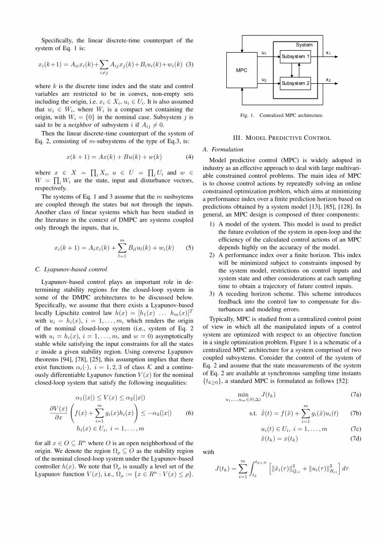
Fig. 1. Centralized MPC architecture.

III. MODEL PREDICTIVE CONTROL

A. Formulation

Model predictive control (MPC) is widely adopted inindustry as an effective approach to deal with large multivari-able constrained control problems. The main idea of MPCis to choose control actions by repeatedly solving an onlineconstrained optimization problem, which aims at minimizinga performance index over a finite prediction horizon based onpredictions obtained by a system model [13], [85], [128]. Ingeneral, an MPC design is composed of three components:

1) A model of the system. This model is used to predictthe future evolution of the system in open-loop and theefficiency of the calculated control actions of an MPCdepends highly on the accuracy of the model.

2) A performance index over a finite horizon. This indexwill be minimized subject to constraints imposed bythe system model, restrictions on control inputs andsystem state and other considerations at each samplingtime to obtain a trajectory of future control inputs.

3) A receding horizon scheme. This scheme introducesfeedback into the control law to compensate for dis-turbances and modeling errors.

Typically, MPC is studied from a centralized control pointof view in which all the manipulated inputs of a controlsystem are optimized with respect to an objective functionin a single optimization problem. Figure 1 is a schematic of acentralized MPC architecture for a system comprised of twocoupled subsystems. Consider the control of the system ofEq. 2 and assume that the state measurements of the systemof Eq. 2 are available at synchronous sampling time instantstk≥0, a standard MPC is formulated as follows [52]:

minu1,...,um∈S(∆)

J(tk) (7a)

s.t. ˙x(t) = f(x) +m∑

i=1

gi(x)ui(t) (7b)

ui(t) ∈ Ui, i = 1, . . . ,m (7c)x(tk) = x(tk) (7d)

with

J(tk) =m∑

i=1

∫ tk+N

tk

[‖xi(τ)‖2Qci

+ ‖ui(τ)‖2Rci

]dτ

where S(∆) is the family of piece-wise constant functionswith sampling period ∆, N is the prediction horizon, Qci

and Rci are strictly positive definite symmetric weightingmatrices, and xi, i = 1, . . . , m, are the predicted trajectoriesof the nominal subsystem i with initial state xi(tk), i =1, . . . ,m, at time tk. The objective of the MPC of Eq.7 isto achieve stabilization of the nominal system of Eq.7 at theorigin, i.e., (x, u) = (0, 0).

The optimal solution to the MPC optimization problemdefined by Eq. 7 is denoted as u∗i (t|tk), i = 1, . . . , m, and isdefined for t ∈ [tk, tk+N ). The first step values of u∗i (t|tk),i = 1, . . . ,m, are applied to the closed-loop system fort ∈ [tk, tk+1). At the next sampling time tk+1, when newmeasurements of the system states xi(tk+1), i = 1, . . . , m,are available, the control evaluation and implementationprocedure is repeated. The manipulated inputs of the systemof Eq. 2 under the control of the MPC of Eq. 7 are definedas follows:

ui(t) = u∗i (t|tk), ∀t ∈ [tk, tk+1), i = 1, . . . , m (8)

which is the standard receding horizon scheme.In the MPC formulation of Eq. 7, the constraint of Eq. 7a

defines a performance index or cost index that should beminimized. In addition to penalties on the state and controlactions, the index may also include penalties on other con-siderations; for example, the rate of change of the inputs.The constraint of Eq. 7b is the nominal model, that is, theuncertainties are supposed to be zero in the model of Eq. 2which is used in the MPC to predict the future evolutionof the process. The constraint of Eq. 7c takes into accountthe constraints on the control inputs, and the constraint ofEq. 7d provides the initial state for the MPC which is ameasurement of the actual system state. Note that in theabove MPC formulation, state constraints are not consideredbut can be readily taken into account.

B. Stability

It is well known that the MPC of Eq. 7 is not neces-sarily stabilizing. To achieve closed-loop stability, differentapproaches have been proposed in the literature. One classof approaches is to use infinite prediction horizons or well-designed terminal penalty terms; please see [12], [96] forsurveys of these approaches. Another class of approachesis to impose stability constraints in the MPC optimizationproblem (e.g.,[18], [96]). There are also efforts focusing ongetting explicit stabilizing MPC laws using offline computa-tions [86]. However, the implicit nature of MPC control lawmakes it very difficult to explicitly characterize, a priori, theadmissible initial conditions starting from where the MPCis guaranteed to be feasible and stabilizing. In practice, theinitial conditions are usually chosen in an ad hoc fashionand tested through extensive closed-loop simulations. Toaddress this issue, Lyapunov-based MPC (LMPC) designshave been proposed in [102], [103] which allow for anexplicit characterization of the stability region and guaranteecontroller feasibility and closed-loop stability. Below wereview various methods for ensuring closed-loop stability

under MPC that are utilized in the DMPC results to bediscussed in the following sections.

We start with stabilizing MPC formulations for lineardiscrete-time systems based on terminal weight and termi-nal constraints. Specifically, a standard centralized MPC isformulated as follows:

minu(k),...,u(k+N−1)

J(k) (9)

subject to Eq. (4) with w = 0 and, for j = 0, . . . , N − 1,

u(k + j) ∈ U , j ≥ 0 (10)x(k + j) ∈ X , j > 0 (11)x(k + N) ∈ Xf (12)

with

J(k) =N−1∑

j=0

[‖x(k + j)‖2Q + ‖u(k + j)‖2R] + Vf (x(k + N))

(13)The optimal solution is denoted u∗(k), . . . , u∗(k + N − 1).At each sampling time, the corresponding first step valuesu∗i (k) are applied following a receding horizon approach.

The terminal set Xf ⊆ X and the terminal cost Vf areused to guarantee stability properties, and can be selectedaccording to the following simple procedure. First, assumethat a linear stabilizing control law

u(k) = Kx(k) (14)

is known in the unconstrained case, i.e. A+BK is stable; awise choice is to compute the gain K as the solution of aninfinite-horizon linear quadratic (LQ) control problem withthe same weights Q and R used in Eq. 13. Then, letting Pbe the solution of the Lyapunov equation

(A + BK)′P (A + BK)− P = −(Q + K ′RK) (15)

it is possible to set Vf = x′Px and Xf = x|x′Px ≤ c,where c is a small positive value chosen so that u = Kx ∈ Ufor any x ∈ Xf . These choices implicitly guarantee adecreasing property of the optimal cost function (similar tothe one explicitly expressed by the constraint of Eq. 16ebelow in the context of Lyapunov-based MPC), so thatthe origin of the state space is an asymptotically stableequilibrium with a region of attraction given by the set ofthe states for which a feasible solution of the optimizationproblem exists, see, for example, [96]. Many other choicesof the design parameters guaranteeing stability properties forlinear and nonlinear systems have been proposed see, forexample, [97], [33], [89], [90], [50], [109], [56], [53].

In addition to stabilizing MPC formulations based onterminal weight and terminal constraints, we also reviewa formulation using Lyapunov function-based stability con-straints since it is utilized in some of the DMPC schemesto be presented below. Specifically, we review the LMPCdesign proposed in [102], [103] which allows for an explicitcharacterization of the stability region and guarantees con-troller feasibility and closed-loop stability. For the predictivecontrol of the system of Eq. 2, the LMPC is designed based

on an existing explicit control law h(x) which is able tostabilize the closed-loop system and satisfies the conditionsof Eq. 6. The formulation of the LMPC is as follows:

minu1,...,um∈S(∆)

J(tk) (16a)

s.t. ˙x(t) = f(x) +m∑

i=1

gi(x)ui(t) (16b)

u(t) ∈ U (16c)x(tk) = x(tk) (16d)∂V (x(tk))

∂xgi(x(tk))ui(tk)

≤ ∂V (x(tk))∂x

gi(x(tk))hi(x(tk)) (16e)

where V (x) is a Lyapunov function associated with thenonlinear control law h(x). The optimal solution to thisLMPC optimization problem is denoted as ul,∗

i (t|tk) whichis defined for t ∈ [tk, tk+N ). The manipulated input of thesystem of Eq. 2 under the control of the LMPC of Eq. 16 isdefined as follows:

ui(t) = ul,∗i (t|tk), ∀t ∈ [tk, tk+1) (17)

which implies that this LMPC also adopts a standard reced-ing horizon strategy.

In the LMPC defined by Eq. 16, the constraint of Eq. 16eguarantees that the value of the time derivative of theLyapunov function, V (x), at time tk is smaller than or equalto the value obtained if the nonlinear control law u = h(x)is implemented in the closed-loop system in a sample-and-hold fashion. This is a constraint that allows one to prove(when state measurements are available every synchronoussampling time) that the LMPC inherits the stability androbustness properties of the nonlinear control law h(x) whenit is applied in a sample-and-hold fashion. Specifically, oneof the main properties of the LMPC of Eq. 16 is thatit possesses the same stability region Ωρ as the nonlinearcontrol law h(x), which implies that the origin of the closed-loop system is guaranteed to be stable and the LMPC isguaranteed to be feasible for any initial state inside Ωρ whenthe sampling time ∆ and the disturbance upper bound θare sufficiently small. The stability property of the LMPCis inherited from the nonlinear control law h(x) when itis applied in a sample-and-hold fashion; please see [28],[110] for results on sampled-data systems. The feasibilityproperty of the LMPC is also guaranteed by the nonlinearcontrol law h(x) since u = h(x) is a feasible solution to theoptimization problem of Eq. 16 (see also [102], [103], [92]for detailed results on this issue). The main advantage ofthe LMPC approach with respect to the nonlinear controllaw h(x) is that optimality considerations can be takenexplicitly into account (as well as constraints on the inputsand the states [103]) in the computation of the control actionswithin an online optimization framework while improvingthe closed-loop performance of the system. We finally notethat since the closed-loop stability and feasibility of theLMPC of Eq. 16 are guaranteed by the nonlinear control

CSTR-4

Fr1

Separator

F7

CSTR-1 CSTR-2 CSTR-3

F1, A

Fr2

F3 F5

F9

F10, D

Q1 Q2 Q3

Q5 Q4

F2, B F4, B F6, B

F8

FPFr

Fig. 2. Alkylation of benzene with ethylene process.

law h(x), it is unnecessary to use a terminal penalty termin the cost index and the length of the horizon N does notaffect the stability of the closed-loop system but it affectsthe closed-loop performance.

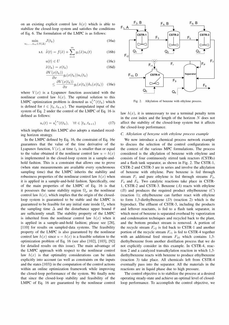
C. Alkylation of benzene with ethylene process example

We now introduce a chemical process network exampleto discuss the selection of the control configurations inthe context of the various MPC formulations. The processconsidered is the alkylation of benzene with ethylene andconsists of four continuously stirred tank reactors (CSTRs)and a flash tank separator, as shown in Fig. 2. The CSTR-1,CSTR-2 and CSTR-3 are in series and involve the alkylationof benzene with ethylene. Pure benzene is fed throughstream F1 and pure ethylene is fed through streams F2,F4 and F6. Two catalytic reactions take place in CSTR-1, CSTR-2 and CSTR-3. Benzene (A) reacts with ethylene(B) and produces the required product ethylbenzene (C)(reaction 1); ethylbenzene can further react with ethyleneto form 1,3-diethylbenzene (D) (reaction 2) which is thebyproduct. The effluent of CSTR-3, including the productsand leftover reactants, is fed to a flash tank separator, inwhich most of benzene is separated overhead by vaporizationand condensation techniques and recycled back to the plant,and the bottom product stream is removed. A portion ofthe recycle stream Fr2 is fed back to CSTR-1 and anotherportion of the recycle stream Fr1 is fed to CSTR-4 togetherwith an additional feed stream F10 which contains 1,3-diethylbenzene from another distillation process that we donot explicitly consider in this example. In CSTR-4, reac-tion 2 and a catalyzed transalkylation reaction in which 1,3-diethylbenzene reacts with benzene to produce ethylbenzene(reaction 3) take place. All chemicals left from CSTR-4eventually pass into the separator. All the materials in thereactions are in liquid phase due to high pressure.

The control objective is to stabilize the process at a desiredoperating steady-state and achieve an optimal level of closed-loop performance. To accomplish the control objective, we

CSTR-4

Fr1

Separator

F7

CSTR-1 CSTR-2 CSTR-3

F1, A

Fr2

F3 F5

F9

F10, D

Q2 Q3

Q5 Q4

F2, B

F4, BF6, B

F8

FPFr

S S S

S

S

MPC

Q1

Plant-wide Network

S : Sensors

x1, x2, …, xm

x1, x2, …, xm

x1, x2, …, xm

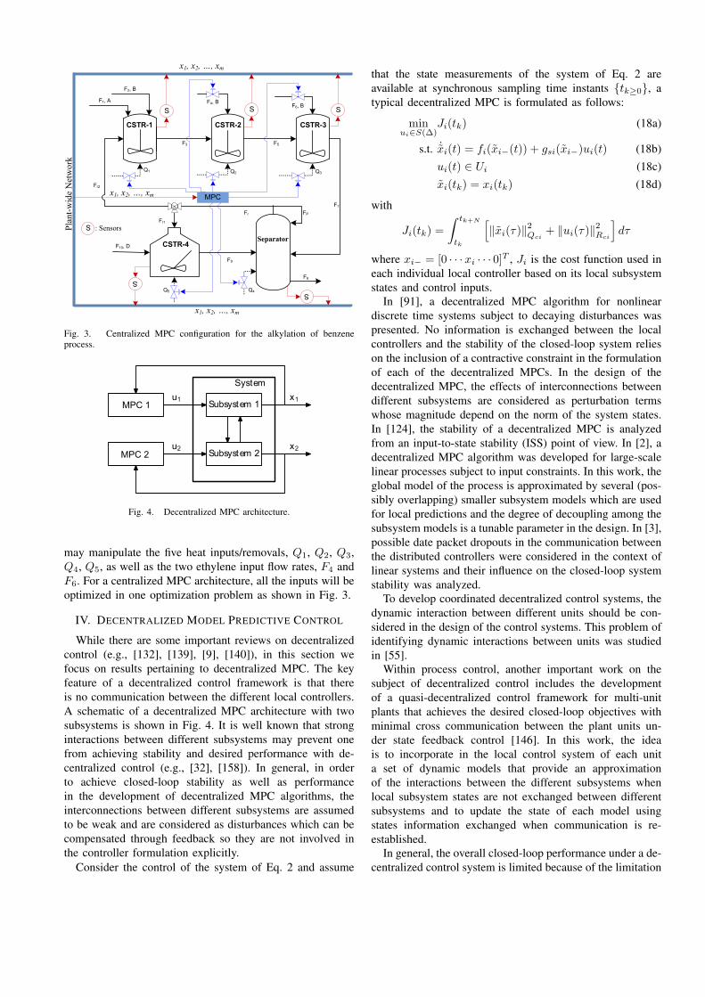
Fig. 3. Centralized MPC configuration for the alkylation of benzeneprocess.

System

MPC 1

MPC 2

Subsystem 1

Subsystem 2

u1

u2

x1

x2

Fig. 4. Decentralized MPC architecture.

may manipulate the five heat inputs/removals, Q1, Q2, Q3,Q4, Q5, as well as the two ethylene input flow rates, F4 andF6. For a centralized MPC architecture, all the inputs will beoptimized in one optimization problem as shown in Fig. 3.

IV. DECENTRALIZED MODEL PREDICTIVE CONTROL

While there are some important reviews on decentralizedcontrol (e.g., [132], [139], [9], [140]), in this section wefocus on results pertaining to decentralized MPC. The keyfeature of a decentralized control framework is that thereis no communication between the different local controllers.A schematic of a decentralized MPC architecture with twosubsystems is shown in Fig. 4. It is well known that stronginteractions between different subsystems may prevent onefrom achieving stability and desired performance with de-centralized control (e.g., [32], [158]). In general, in orderto achieve closed-loop stability as well as performancein the development of decentralized MPC algorithms, theinterconnections between different subsystems are assumedto be weak and are considered as disturbances which can becompensated through feedback so they are not involved inthe controller formulation explicitly.

Consider the control of the system of Eq. 2 and assume

that the state measurements of the system of Eq. 2 areavailable at synchronous sampling time instants tk≥0, atypical decentralized MPC is formulated as follows:

minui∈S(∆)

Ji(tk) (18a)

s.t. ˙xi(t) = fi(xi−(t)) + gsi(xi−)ui(t) (18b)ui(t) ∈ Ui (18c)xi(tk) = xi(tk) (18d)

with

Ji(tk) =∫ tk+N

tk

[‖xi(τ)‖2Qci

+ ‖ui(τ)‖2Rci

]dτ

where xi− = [0 · · ·xi · · · 0]T , Ji is the cost function used ineach individual local controller based on its local subsystemstates and control inputs.

In [91], a decentralized MPC algorithm for nonlineardiscrete time systems subject to decaying disturbances waspresented. No information is exchanged between the localcontrollers and the stability of the closed-loop system relieson the inclusion of a contractive constraint in the formulationof each of the decentralized MPCs. In the design of thedecentralized MPC, the effects of interconnections betweendifferent subsystems are considered as perturbation termswhose magnitude depend on the norm of the system states.In [124], the stability of a decentralized MPC is analyzedfrom an input-to-state stability (ISS) point of view. In [2], adecentralized MPC algorithm was developed for large-scalelinear processes subject to input constraints. In this work, theglobal model of the process is approximated by several (pos-sibly overlapping) smaller subsystem models which are usedfor local predictions and the degree of decoupling among thesubsystem models is a tunable parameter in the design. In [3],possible date packet dropouts in the communication betweenthe distributed controllers were considered in the context oflinear systems and their influence on the closed-loop systemstability was analyzed.

To develop coordinated decentralized control systems, thedynamic interaction between different units should be con-sidered in the design of the control systems. This problem ofidentifying dynamic interactions between units was studiedin [55].

Within process control, another important work on thesubject of decentralized control includes the developmentof a quasi-decentralized control framework for multi-unitplants that achieves the desired closed-loop objectives withminimal cross communication between the plant units un-der state feedback control [146]. In this work, the ideais to incorporate in the local control system of each unita set of dynamic models that provide an approximationof the interactions between the different subsystems whenlocal subsystem states are not exchanged between differentsubsystems and to update the state of each model usingstates information exchanged when communication is re-established.

In general, the overall closed-loop performance under a de-centralized control system is limited because of the limitation

CSTR-4

Fr1

Separator

F7

CSTR-1 CSTR-2 CSTR-3

F1, A

Fr2

F3 F5

F9

F10, D

Q2 Q3

Q5 Q4

F2, B

F4, BF6, B

F8

FPFr

S S S

S

S

MPC 2

Q1

S : Sensors

MPC 1

MPC 3

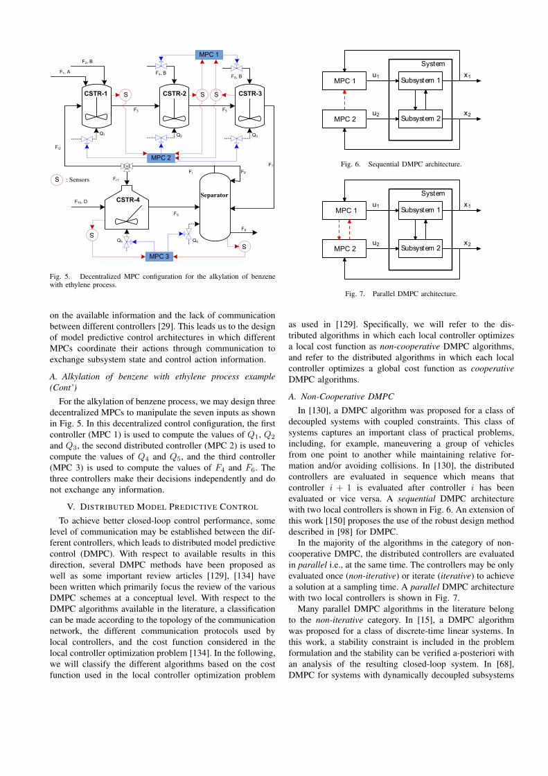
Fig. 5. Decentralized MPC configuration for the alkylation of benzenewith ethylene process.

on the available information and the lack of communicationbetween different controllers [29]. This leads us to the designof model predictive control architectures in which differentMPCs coordinate their actions through communication toexchange subsystem state and control action information.

A. Alkylation of benzene with ethylene process example(Cont’)

For the alkylation of benzene process, we may design threedecentralized MPCs to manipulate the seven inputs as shownin Fig. 5. In this decentralized control configuration, the firstcontroller (MPC 1) is used to compute the values of Q1, Q2

and Q3, the second distributed controller (MPC 2) is used tocompute the values of Q4 and Q5, and the third controller(MPC 3) is used to compute the values of F4 and F6. Thethree controllers make their decisions independently and donot exchange any information.

V. DISTRIBUTED MODEL PREDICTIVE CONTROL

To achieve better closed-loop control performance, somelevel of communication may be established between the dif-ferent controllers, which leads to distributed model predictivecontrol (DMPC). With respect to available results in thisdirection, several DMPC methods have been proposed aswell as some important review articles [129], [134] havebeen written which primarily focus the review of the variousDMPC schemes at a conceptual level. With respect to theDMPC algorithms available in the literature, a classificationcan be made according to the topology of the communicationnetwork, the different communication protocols used bylocal controllers, and the cost function considered in thelocal controller optimization problem [134]. In the following,we will classify the different algorithms based on the costfunction used in the local controller optimization problem

System

MPC 1

MPC 2

Subsystem 1

Subsystem 2

u1

u2

x1

x2

Fig. 6. Sequential DMPC architecture.

System

MPC 1

MPC 2

Subsystem 1

Subsystem 2

u1

u2

x1

x2

Fig. 7. Parallel DMPC architecture.

as used in [129]. Specifically, we will refer to the dis-tributed algorithms in which each local controller optimizesa local cost function as non-cooperative DMPC algorithms,and refer to the distributed algorithms in which each localcontroller optimizes a global cost function as cooperativeDMPC algorithms.

A. Non-Cooperative DMPC

In [130], a DMPC algorithm was proposed for a class ofdecoupled systems with coupled constraints. This class ofsystems captures an important class of practical problems,including, for example, maneuvering a group of vehiclesfrom one point to another while maintaining relative for-mation and/or avoiding collisions. In [130], the distributedcontrollers are evaluated in sequence which means thatcontroller i + 1 is evaluated after controller i has beenevaluated or vice versa. A sequential DMPC architecturewith two local controllers is shown in Fig. 6. An extension ofthis work [150] proposes the use of the robust design methoddescribed in [98] for DMPC.

In the majority of the algorithms in the category of non-cooperative DMPC, the distributed controllers are evaluatedin parallel i.e., at the same time. The controllers may be onlyevaluated once (non-iterative) or iterate (iterative) to achievea solution at a sampling time. A parallel DMPC architecturewith two local controllers is shown in Fig. 7.

Many parallel DMPC algorithms in the literature belongto the non-iterative category. In [15], a DMPC algorithmwas proposed for a class of discrete-time linear systems. Inthis work, a stability constraint is included in the problemformulation and the stability can be verified a-posteriori withan analysis of the resulting closed-loop system. In [68],DMPC for systems with dynamically decoupled subsystems

(a class of systems of relevance in the context of multi-agents systems) where the cost function and constraintscouple the dynamical behavior of the system. The couplingin the system is described using a graph in which eachsubsystem is a node. It is assumed that each subsystemcan exchange information with its neighbors (a subset ofother subsystems). Based on the results of [68], a DMPCframework was constructed for control and coordination ofautonomous vehicle teams [69].

In [64], a DMPC scheme for linear systems coupledonly through the state is considered, while [38] deals withthe problem of distributed control of dynamically decou-pled nonlinear systems coupled by their cost function. Thismethod is extended to the case of dynamically couplednonlinear systems in [36] and applied as a distributed controlstrategy in the context of supply chain optimization in [37].In this implementation, the agents optimize locally theirown policy, which is communicated to their neighbors. Thestability is assured through a compatibility constraint: theagents commit themselves not to deviate too far in theirstate and input trajectories from what their neighbors believethey plan to do. In [100] another iterative implementationof a similar DMPC scheme was applied together with adistributed Kalman filter to a quadruple tank system. Finally,in [76] the Shell benchmark problem is used to test a similaralgorithm. Note that all these methods lead in general toNash equilibria as long as the cost functions of the agentsare selfish.

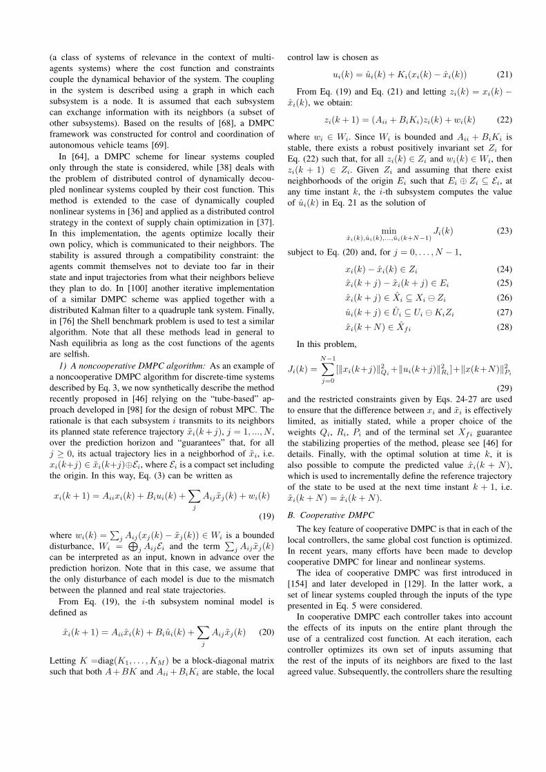
1) A noncooperative DMPC algorithm: As an example ofa noncooperative DMPC algorithm for discrete-time systemsdescribed by Eq. 3, we now synthetically describe the methodrecently proposed in [46] relying on the “tube-based” ap-proach developed in [98] for the design of robust MPC. Therationale is that each subsystem i transmits to its neighborsits planned state reference trajectory xi(k + j), j = 1, ..., N ,over the prediction horizon and “guarantees” that, for allj ≥ 0, its actual trajectory lies in a neighborhod of xi, i.e.xi(k+j) ∈ xi(k+j)⊕Ei, where Ei is a compact set includingthe origin. In this way, Eq. (3) can be written as

xi(k + 1) = Aiixi(k) + Biui(k) +∑

j

Aij xj(k) + wi(k)

(19)

where wi(k) =∑

j Aij(xj(k) − xj(k)) ∈ Wi is a boundeddisturbance, Wi =

⊕j AijEi and the term

∑j Aij xj(k)

can be interpreted as an input, known in advance over theprediction horizon. Note that in this case, we assume thatthe only disturbance of each model is due to the mismatchbetween the planned and real state trajectories.

From Eq. (19), the i-th subsystem nominal model isdefined as

xi(k + 1) = Aiixi(k) + Biui(k) +∑

j

Aij xj(k) (20)

Letting K =diag(K1, . . . ,KM ) be a block-diagonal matrixsuch that both A+BK and Aii +BiKi are stable, the local

control law is chosen as

ui(k) = ui(k) + Ki(xi(k)− xi(k)) (21)

From Eq. (19) and Eq. (21) and letting zi(k) = xi(k) −xi(k), we obtain:

zi(k + 1) = (Aii + BiKi)zi(k) + wi(k) (22)

where wi ∈ Wi. Since Wi is bounded and Aii + BiKi isstable, there exists a robust positively invariant set Zi forEq. (22) such that, for all zi(k) ∈ Zi and wi(k) ∈ Wi, thenzi(k + 1) ∈ Zi. Given Zi and assuming that there existneighborhoods of the origin Ei such that Ei ⊕ Zi ⊆ Ei, atany time instant k, the i-th subsystem computes the valueof ui(k) in Eq. 21 as the solution of

minxi(k),ui(k),...,ui(k+N−1)

Ji(k) (23)

subject to Eq. (20) and, for j = 0, . . . , N − 1,

xi(k)− xi(k) ∈ Zi (24)xi(k + j)− xi(k + j) ∈ Ei (25)

xi(k + j) ∈ Xi ⊆ Xi ª Zi (26)

ui(k + j) ∈ Ui ⊆ Ui ªKiZi (27)

xi(k + N) ∈ Xfi (28)

In this problem,

Ji(k) =N−1∑

j=0

[‖xi(k+j)‖2Qi+‖ui(k+j)‖2Ri

]+‖x(k+N)‖2Pi

(29)and the restricted constraints given by Eqs. 24-27 are usedto ensure that the difference between xi and xi is effectivelylimited, as initially stated, while a proper choice of theweights Qi, Ri, Pi and of the terminal set Xfi guaranteethe stabilizing properties of the method, please see [46] fordetails. Finally, with the optimal solution at time k, it isalso possible to compute the predicted value xi(k + N),which is used to incrementally define the reference trajectoryof the state to be used at the next time instant k + 1, i.e.xi(k + N) = xi(k + N).

B. Cooperative DMPC

The key feature of cooperative DMPC is that in each of thelocal controllers, the same global cost function is optimized.In recent years, many efforts have been made to developcooperative DMPC for linear and nonlinear systems.

The idea of cooperative DMPC was first introduced in[154] and later developed in [129]. In the latter work, aset of linear systems coupled through the inputs of the typepresented in Eq. 5 were considered.

In cooperative DMPC each controller takes into accountthe effects of its inputs on the entire plant through theuse of a centralized cost function. At each iteration, eachcontroller optimizes its own set of inputs assuming thatthe rest of the inputs of its neighbors are fixed to the lastagreed value. Subsequently, the controllers share the resulting

optimal trajectories and a final optimal trajectory is computedat each sampling time as a weighted sum of the most recentoptimal trajectories with the optimal trajectories computedat the last sampling time.

The cooperative DMPCs use the following implementationstrategy:

1. At k, all the controllers receive the full state measure-ment x(k) from the sensors.

2. At iteration c (c ≥ 1):2.1. Each controller evaluates its own future input tra-

jectory based on x(k) and the latest received in-put trajectories of all the other controllers (whenc = 1, initial input guesses obtained from theshifted latest optimal input trajectories are used).

2.2. The controllers exchange their future input tra-jectories. Based on all the input trajectories, eachcontroller calculates the current decided set ofinputs trajectories uc.

3. If a termination condition is satisfied, each controllersends its entire future input trajectory to its actuators;if the termination condition is not satisfied, go to Step2 (c ← c + 1).

4. When a new measurement is received, go to Step 1(k ← k + 1).

At each iteration, each controller solves the followingoptimization problem:

minui(k),...,ui(k+N−1)

J(k) (30)

subject to Eq. (4) with w = 0 and, for j = 0, . . . , N − 1,

ui(k + j) ∈ Ui , j ≥ 0 (31)

ul(k + j) = ul(k + j)c−1 ,∀l 6= i (32)x(k + j) ∈ X , j > 0 (33)x(k + N) ∈ Xf (34)

withJ(k) =

∑

i

Ji(k) (35)

and

Ji(k) =N−1∑

j=0

[‖xi(k+j)‖2Qi+‖ui(k+j)‖2Ri

]+‖x(k+N)‖2Pi

(36)Note that each controller must have knowledge of the fullsystem dynamics and of the overall objective function.

After the controllers share the optimal solutions ui(k+j)∗,the optimal trajectory at iteration c, ui(k + j)c, is obtainedfrom a convex combination between the last optimal solutionand the current optimal solution of the MPC problem of eachcontroller, that is,

ui(k + j)c = αiui(k + j)c−1 + (1− αi)ui(k + j)∗

where αi are the weighting factors for each agent. Thisdistributed optimization is of the Gauss-Jacobi type.

In [154], [143], an iterative cooperative DMPC algorithmwas designed for linear systems. It was proven that through

Process

LMPC 1

LMPC 2

LMPC m − 1

LMPC m

Sensors

x

x

um

um−1

.

.

.

u2

u1

um

.

.

.

um, um−1

um, . . . , u3

um, . . . , u2

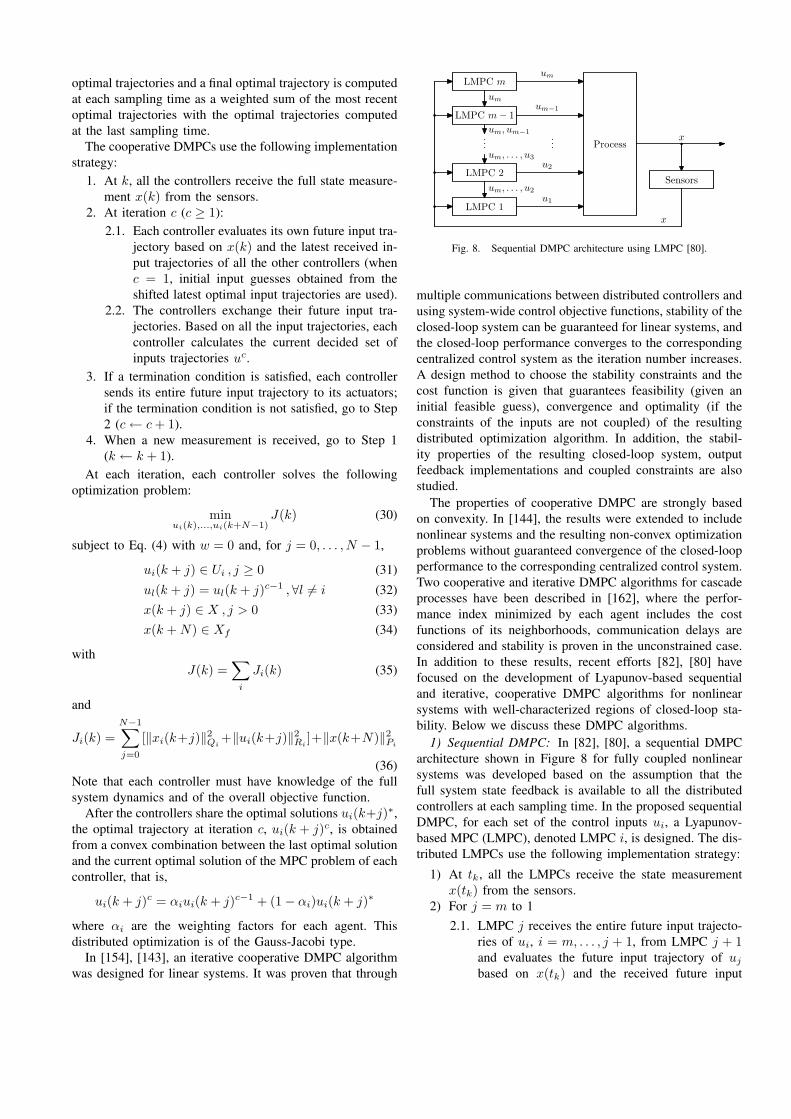
Fig. 8. Sequential DMPC architecture using LMPC [80].

multiple communications between distributed controllers andusing system-wide control objective functions, stability of theclosed-loop system can be guaranteed for linear systems, andthe closed-loop performance converges to the correspondingcentralized control system as the iteration number increases.A design method to choose the stability constraints and thecost function is given that guarantees feasibility (given aninitial feasible guess), convergence and optimality (if theconstraints of the inputs are not coupled) of the resultingdistributed optimization algorithm. In addition, the stabil-ity properties of the resulting closed-loop system, outputfeedback implementations and coupled constraints are alsostudied.

The properties of cooperative DMPC are strongly basedon convexity. In [144], the results were extended to includenonlinear systems and the resulting non-convex optimizationproblems without guaranteed convergence of the closed-loopperformance to the corresponding centralized control system.Two cooperative and iterative DMPC algorithms for cascadeprocesses have been described in [162], where the perfor-mance index minimized by each agent includes the costfunctions of its neighborhoods, communication delays areconsidered and stability is proven in the unconstrained case.In addition to these results, recent efforts [82], [80] havefocused on the development of Lyapunov-based sequentialand iterative, cooperative DMPC algorithms for nonlinearsystems with well-characterized regions of closed-loop sta-bility. Below we discuss these DMPC algorithms.

1) Sequential DMPC: In [82], [80], a sequential DMPCarchitecture shown in Figure 8 for fully coupled nonlinearsystems was developed based on the assumption that thefull system state feedback is available to all the distributedcontrollers at each sampling time. In the proposed sequentialDMPC, for each set of the control inputs ui, a Lyapunov-based MPC (LMPC), denoted LMPC i, is designed. The dis-tributed LMPCs use the following implementation strategy:

1) At tk, all the LMPCs receive the state measurementx(tk) from the sensors.

2) For j = m to 12.1. LMPC j receives the entire future input trajecto-

ries of ui, i = m, . . . , j + 1, from LMPC j + 1and evaluates the future input trajectory of uj

based on x(tk) and the received future input

trajectories.2.2. LMPC j sends the first step input value of uj to

its actuators and the entire future input trajecto-ries of ui, i = m, . . . , j, to LMPC j − 1.

3) When a new measurement is received (k ← k +1), goto Step 1.

In this architecture, each LMPC only sends its futureinput trajectory and the future input trajectories it receivedto the next LMPC (i.e., LMPC j sends input trajectories toLMPC j − 1). This implies that LMPC j, j = m, . . . , 2,does not have any information about the values that ui,i = j − 1, . . . , 1 will take when the optimization problemsof the LMPCs are designed. In order to make a decision,LMPC j, j = m, . . . , 2 must assume trajectories for ui,i = j−1, . . . , 1, along the prediction horizon. To this end, anexplicit nonlinear control law h(x) which can stabilize theclosed-loop system asymptotically is used. In order to inheritthe stability properties of the controller h(x), a Lyapunovfunction based constraint is incorporated in each LMPC toguarantee a given minimum contribution to the decreaserate of the Lyapunov function V (x). Specifically, the designof LMPC j, j = 1, . . . , m, is based on the followingoptimization problem:

minuj∈S(∆)

J(tk) (37a)

s.t. ˙x(t) = f(x(t)) +m∑

i=1

gi(x(t))ui (37b)

ui(t) = hi(x(tk+l)), i = 1, . . . , j − 1,

∀t ∈ [tk+l, tk+l+1), l = 0, ..., N − 1 (37c)ui(t) = u∗s,i(t|tk), i = j + 1, . . . , m (37d)

uj(t) ∈ Uj (37e)x(tk) = x(tk) (37f)∂V (x(tk))

∂xgj(x(tk))uj(tk)

≤ ∂V (x(tk))∂x

gj(x(tk))hj(x(tk)). (37g)

In the optimization problem of Eq. 37, u∗s,i(t|tk) denotesthe optimal future input trajectory of ui obtained by LMPC ievaluated before LMPC j. The constraint of Eq. 37c definesthe value of the inputs evaluated after uj (i.e., ui with i =1, . . . , j − 1); the constraint of Eq. 37d defines the value ofthe inputs evaluated before uj (i.e., ui with i = j+1, . . . ,m);the constraint of Eq. 37g guarantees that the contribution ofinput uj to the decrease rate of the time derivative of theLyapunov function V (x) at the initial evaluation time (i.e.,at tk), if uj = u∗s,j(tk|tk) is applied, is bigger than or equalto the value obtained when uj = hj(x(tk)) is applied. Thisconstraint allows proving the closed-loop stability propertiesof this DMPC [82], [80].

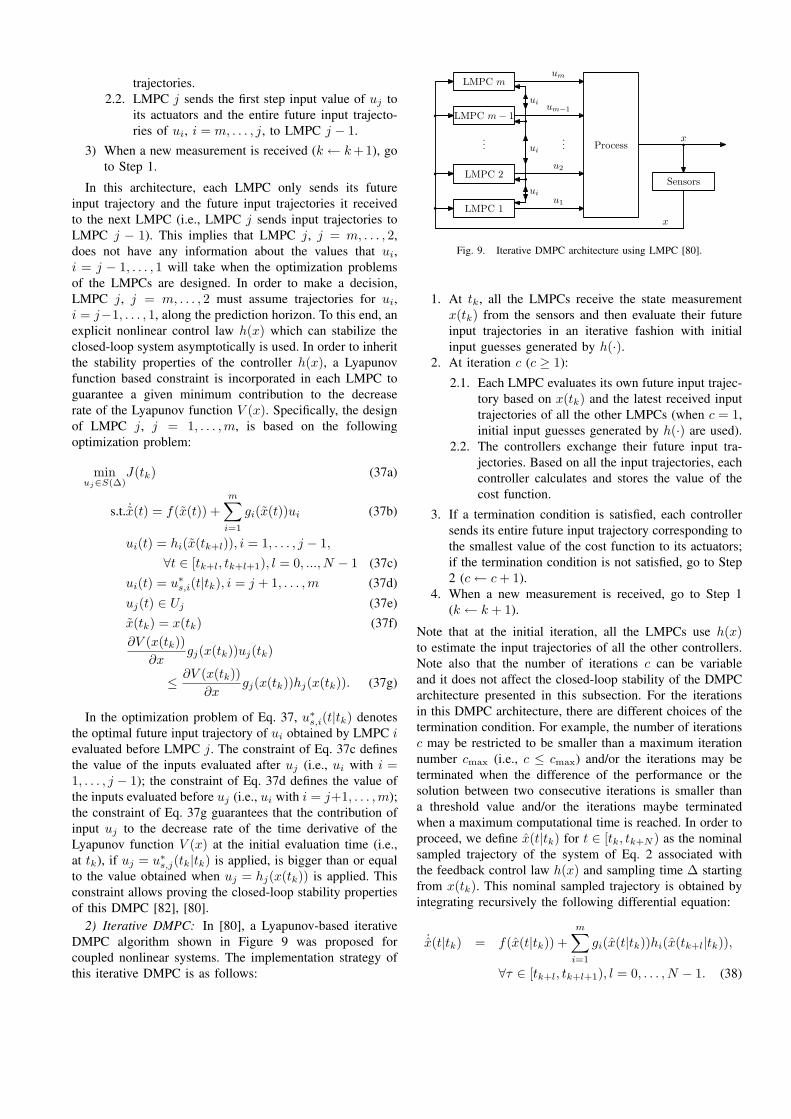
2) Iterative DMPC: In [80], a Lyapunov-based iterativeDMPC algorithm shown in Figure 9 was proposed forcoupled nonlinear systems. The implementation strategy ofthis iterative DMPC is as follows:

Process

LMPC 1

LMPC 2

LMPC m − 1

LMPC m

Sensors

x

x

um

um−1

.

.

....

u2

u1

ui

ui

ui

Fig. 9. Iterative DMPC architecture using LMPC [80].

1. At tk, all the LMPCs receive the state measurementx(tk) from the sensors and then evaluate their futureinput trajectories in an iterative fashion with initialinput guesses generated by h(·).

2. At iteration c (c ≥ 1):

2.1. Each LMPC evaluates its own future input trajec-tory based on x(tk) and the latest received inputtrajectories of all the other LMPCs (when c = 1,initial input guesses generated by h(·) are used).

2.2. The controllers exchange their future input tra-jectories. Based on all the input trajectories, eachcontroller calculates and stores the value of thecost function.

3. If a termination condition is satisfied, each controllersends its entire future input trajectory corresponding tothe smallest value of the cost function to its actuators;if the termination condition is not satisfied, go to Step2 (c ← c + 1).

4. When a new measurement is received, go to Step 1(k ← k + 1).

Note that at the initial iteration, all the LMPCs use h(x)to estimate the input trajectories of all the other controllers.Note also that the number of iterations c can be variableand it does not affect the closed-loop stability of the DMPCarchitecture presented in this subsection. For the iterationsin this DMPC architecture, there are different choices of thetermination condition. For example, the number of iterationsc may be restricted to be smaller than a maximum iterationnumber cmax (i.e., c ≤ cmax) and/or the iterations may beterminated when the difference of the performance or thesolution between two consecutive iterations is smaller thana threshold value and/or the iterations maybe terminatedwhen a maximum computational time is reached. In order toproceed, we define x(t|tk) for t ∈ [tk, tk+N ) as the nominalsampled trajectory of the system of Eq. 2 associated withthe feedback control law h(x) and sampling time ∆ startingfrom x(tk). This nominal sampled trajectory is obtained byintegrating recursively the following differential equation:

˙x(t|tk) = f(x(t|tk)) +m∑

i=1

gi(x(t|tk))hi(x(tk+l|tk)),

∀τ ∈ [tk+l, tk+l+1), l = 0, . . . , N − 1. (38)

Based on x(t|tk), we can define the following variable:

un,j(t|tk) = hj(x(tk+l|tk)), j = 1, . . . ,m,

∀τ ∈ [tk+l, tk+l+1), l = 0, . . . , N − 1.(39)

which will be used as the initial guess of the trajectory ofuj .

The design of the LMPC j, j = 1, . . . , m, at iteration cis based on the following optimization problem:

minuj∈S(∆)

J(tk) (40a)

s.t. ˙x(t) = f(x(t)) +m∑

i=1

gi(x(t))ui (40b)

ui(t) = u∗,c−1p,i (t|tk), ∀i 6= j (40c)

uj(t) ∈ Uj (40d)x(tk) = x(tk) (40e)∂V (x(tk))

∂xgj(x(tk))uj(tk)

≤ ∂V (x(tk))∂x

gj(x(tk))hj(x(tk)) (40f)

where u∗,c−1p,i (t|tk) is the optimal input trajectories at itera-

tion c− 1.In general, there is no guaranteed convergence of the

optimal cost or solution of an iterated DMPC to the optimalcost or solution of a centralized MPC for general nonlin-ear constrained systems because of the non-convexity ofthe MPC optimization problems. However, with the aboveimplementation strategy of the iterative DMPC presented inthis section, it is guaranteed that the optimal cost of thedistributed optimization of Eq. 40 is upper bounded by thecost of the Lyapunov-based controller h(·) at each samplingtime.

Note that in the case of linear systems, the constraint ofEq. 40f is linear with respect to uj and it can be verifiedthat the optimization problem of Eq. 40 is convex. The inputgiven by LMPC j of Eq. 40 at each iteration may be definedas a convex combination of the current optimal input solutionand the previous one, for example,

ucp,j(t|tk) =

m,i 6=j∑

i=1

wiuc−1p,j (t|tk) + wju

∗,cp,j(t|tk) (41)

wherem∑

i=1

wi = 1 with 0 < wi < 1, u∗,cp,j is the current

solution given by the optimization problem of Eq. 40 anduc−1

p,j is the convex combination of the solutions obtained atiteration c− 1. By doing this, it is possible to prove that theoptimal cost of the distributed LMPC of Eq. 40 convergesto the one of the corresponding centralized control system[11], [143], [26].

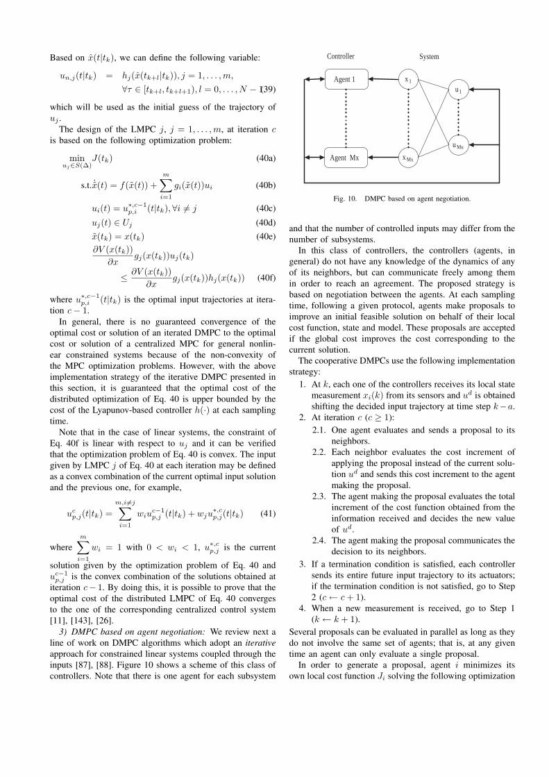
3) DMPC based on agent negotiation: We review next aline of work on DMPC algorithms which adopt an iterativeapproach for constrained linear systems coupled through theinputs [87], [88]. Figure 10 shows a scheme of this class ofcontrollers. Note that there is one agent for each subsystem

x 1

x Mx

u 1

u Mu

Agent 1

Agent Mx

System Controller

Fig. 10. DMPC based on agent negotiation.

and that the number of controlled inputs may differ from thenumber of subsystems.

In this class of controllers, the controllers (agents, ingeneral) do not have any knowledge of the dynamics of anyof its neighbors, but can communicate freely among themin order to reach an agreement. The proposed strategy isbased on negotiation between the agents. At each samplingtime, following a given protocol, agents make proposals toimprove an initial feasible solution on behalf of their localcost function, state and model. These proposals are acceptedif the global cost improves the cost corresponding to thecurrent solution.

The cooperative DMPCs use the following implementationstrategy:

1. At k, each one of the controllers receives its local statemeasurement xi(k) from its sensors and ud is obtainedshifting the decided input trajectory at time step k−a.

2. At iteration c (c ≥ 1):2.1. One agent evaluates and sends a proposal to its

neighbors.2.2. Each neighbor evaluates the cost increment of

applying the proposal instead of the current solu-tion ud and sends this cost increment to the agentmaking the proposal.

2.3. The agent making the proposal evaluates the totalincrement of the cost function obtained from theinformation received and decides the new valueof ud.

2.4. The agent making the proposal communicates thedecision to its neighbors.

3. If a termination condition is satisfied, each controllersends its entire future input trajectory to its actuators;if the termination condition is not satisfied, go to Step2 (c ← c + 1).

4. When a new measurement is received, go to Step 1(k ← k + 1).

Several proposals can be evaluated in parallel as long as theydo not involve the same set of agents; that is, at any giventime an agent can only evaluate a single proposal.

In order to generate a proposal, agent i minimizes itsown local cost function Ji solving the following optimization

problem:

minu(k),...,u(k+N−1)

Ji(k) (42)

subject to Eq. (5) with wi = 0 and, for j = 0, . . . , N − 1,

ul(k + j) ∈ Ul , l ∈ nprop (43)

ul(k + j) = ul(k + j)d ,∀l /∈ nprop (44)xi(k + j) ∈ Xi , j > 0 (45)xi(k + N) ∈ Xfi (46)

where the Ji(k) cost function depends on the predictedtrajectory of xi and the inputs which affect it. In thisoptimization problem, agent i optimizes over a set nprop ofinputs that affect its dynamics. The rest of inputs are set tothe currently accepted solution ul(k + j)d.

Each agent l who is affected by the proposal of agent ievaluates the predicted cost corresponding to the proposedsolution. To do so, the agent calculates the difference be-tween the cost of the new proposal and the cost of thecurrent accepted proposal. This information is sent to agenti, which can then evaluate the total cost of its proposal,that is, J(k) =

∑i Ji(k), to make a cooperative decision

on the future inputs trajectories. If the cost improves thecurrently accepted solution, then ul(k+j)d = ul(k+j)∗ forall l ∈ nprop, else the proposal is discarded.

With an appropriate design of the objective functions,the terminal region constraints and assuming that an initialfeasible solution is at hand, this controller can be shownto provide guaranteed stability of the resulting closed-loopsystem.

C. Distributed optimization

Starting from the seminal contributions reportedin [101], [49], many efforts have been devoted to developmethods for the decomposition of a large optimizationproblem into a number of smaller and more tractable ones.Methods such as primal or dual decomposition are basedon this idea; an extensive review of this kind of algorithmscan be found in [11]. Dual decomposition has been usedfor DMPC in [125], while other augmented lagrangianformulations were proposed in [113] and applied to thecontrol of irrigation canals in [116] and to traffic networks,see [14], [39]. In the MPC framework, algorithms based onthis approach have also been described in [67], [20], [21].A different gradient-based distributed dynamic optimizationmethod was proposed in [136], [137] and applied to anexperimental four tanks plant in [6]. The method of [136],[137] is based on the exchange of sensitivities. Thisinformation is used to modify the local cost function ofeach agent adding a linear term which partially allow toconsider the other agents’ objectives.

In order to present the basic idea underlying the appli-cation of the popular dual decomposition approach in thecontext of MPC, consider the set of systems of Eq. 3 in nom-inal conditions (wi = 0) and the following (unconstrained)problem

minu(k),...,u(k+N−1)

J(k) =m∑

i=1

Ji(k) (47)

where

Ji(k) =N−1∑

j=0

[‖xi(k+j)‖2Qi+‖ui(k+j)‖2Ri

]+‖xi(k+N)‖2Pi

(48)Note that the problem is separable in the cost function

given by Eq. 47, while the coupling between the subproblemsis due to the dynamics of Eq. 3. Define now the “couplingvariables” νi =

∑j 6=i Aijxj and write Eq. 3 as

xi(k + 1) = Aiixi(k) + Biui(k) + νi(k) (49)

Let λi be the Lagrange multipliers, and consider the La-grangian function:

L(k) =m∑

i=1

[Ji(k)+N−1∑

l=0

λi(k+l)(νi(k+l)−∑

j 6=i

Aijxj(k+l))]

(50)For the generic vector variable ϕ, let ϕi(k) =

[ϕ′i(k) , . . . , ϕ

′i(k +N − 1)]

′and ϕ = [ϕ

′1 , . . . , ϕ

′m]

′. Then,

by relaxation of the coupling constraints, the optimizationproblem of Eq. 47 can be stated as

maxλ(k)

minu(k),ν(k)

L(k) (51)

or, equivalently

maxλ(k)

m∑

i=1

Ji(k) (52)

where, letting Aji be a block-diagonal matrix made by Nblocks equal to Aji,

Ji(k) = minui(k),νi(k)

[Ji(k)+ λ′i(k)νi(k)−

∑

j 6=i

λ′j(k)Ajixi(k))]

(53)At any time instant, this optimization problem is solved

according to the following two-step iterative procedure:1) for a fixed λ, solve the set of m independent min-

imization problems given by Eq. 53 with respect toui(k), νi(k);

2) given the collective values of u, ν computed at theprevious step, solve the maximization problem givenby Eq. 52 with respect to λ.

Although the decomposition approaches usually requirea great number of iterations to obtain a solution, manyefforts have been devoted to derive efficient algorithms, seefor example in [11], [112]. Notably, as shown for examplein [35], the second step of the optimization procedure canbe also performed in a distributed way by suitably exploitingthe structure of the problem.

CSTR-4

Fr1

Separator

F7

CSTR-1 CSTR-2 CSTR-3

F1, A

Fr2

F3 F5

F9

F10, D

Q2 Q3

Q5 Q4

F2, B

F4, B F6, B

F8

FPFr

S S S

S

S

MPC 2

Q1

Plant-wide Network

S : Sensors

x1, x2, …, xm, u1, u2, …, un

X, U

x1, x2, …, xm, u1, u2, …, un

u2

MPC 1

u1X, U

MPC 3

u3X, U

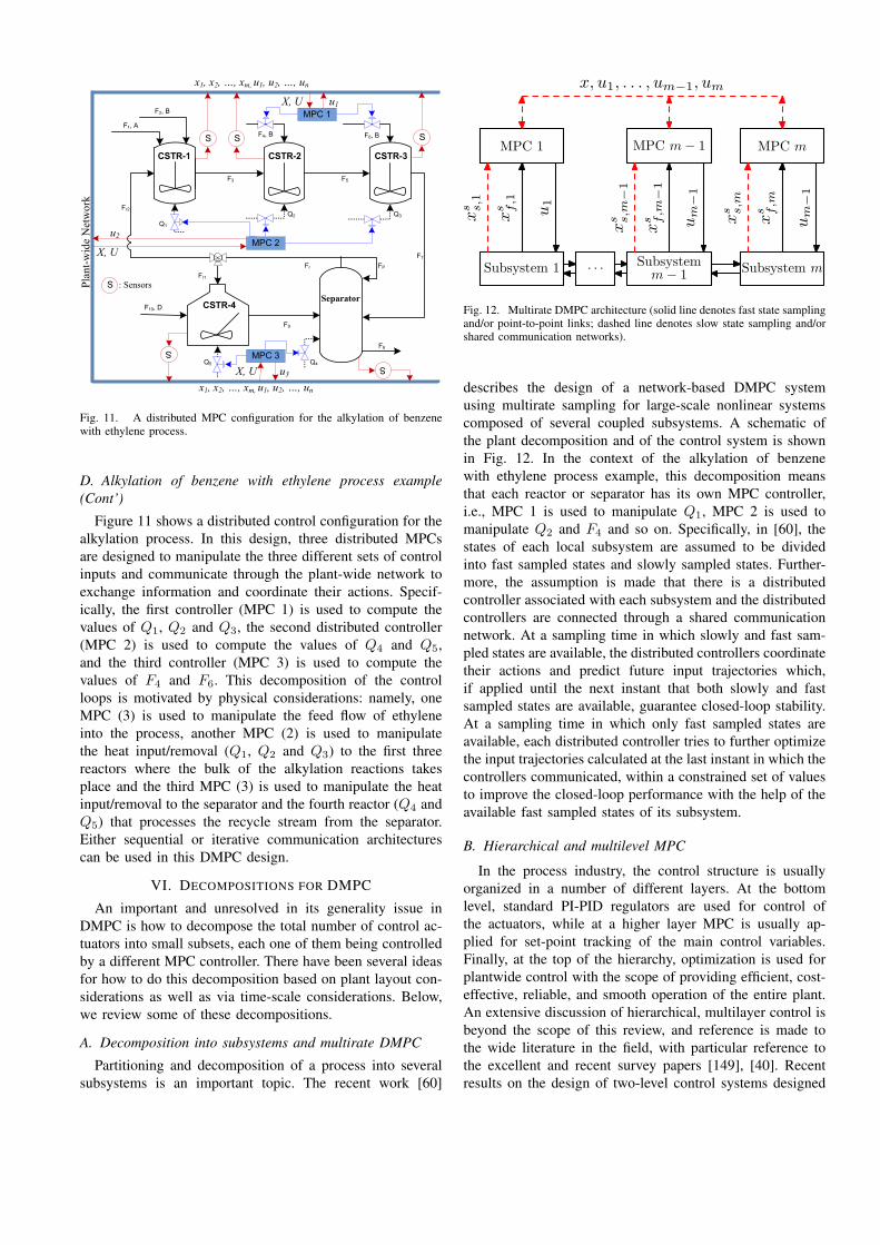
Fig. 11. A distributed MPC configuration for the alkylation of benzenewith ethylene process.

D. Alkylation of benzene with ethylene process example(Cont’)

Figure 11 shows a distributed control configuration for thealkylation process. In this design, three distributed MPCsare designed to manipulate the three different sets of controlinputs and communicate through the plant-wide network toexchange information and coordinate their actions. Specif-ically, the first controller (MPC 1) is used to compute thevalues of Q1, Q2 and Q3, the second distributed controller(MPC 2) is used to compute the values of Q4 and Q5,and the third controller (MPC 3) is used to compute thevalues of F4 and F6. This decomposition of the controlloops is motivated by physical considerations: namely, oneMPC (3) is used to manipulate the feed flow of ethyleneinto the process, another MPC (2) is used to manipulatethe heat input/removal (Q1, Q2 and Q3) to the first threereactors where the bulk of the alkylation reactions takesplace and the third MPC (3) is used to manipulate the heatinput/removal to the separator and the fourth reactor (Q4 andQ5) that processes the recycle stream from the separator.Either sequential or iterative communication architecturescan be used in this DMPC design.

VI. DECOMPOSITIONS FOR DMPC

An important and unresolved in its generality issue inDMPC is how to decompose the total number of control ac-tuators into small subsets, each one of them being controlledby a different MPC controller. There have been several ideasfor how to do this decomposition based on plant layout con-siderations as well as via time-scale considerations. Below,we review some of these decompositions.

A. Decomposition into subsystems and multirate DMPC

Partitioning and decomposition of a process into severalsubsystems is an important topic. The recent work [60]

MPC 1

Subsystem 1

MPC m− 1

Subsystemm− 1

MPC m

Subsystem m· · ·

xs s,1

xs f,1

u1

xs s,m

−1

xs f,m

−1

um

−1

xs s,m

xs f,m

um

−1

x, u1, . . . , um−1, um

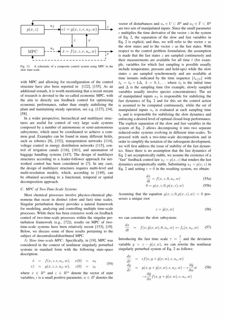
Fig. 12. Multirate DMPC architecture (solid line denotes fast state samplingand/or point-to-point links; dashed line denotes slow state sampling and/orshared communication networks).

describes the design of a network-based DMPC systemusing multirate sampling for large-scale nonlinear systemscomposed of several coupled subsystems. A schematic ofthe plant decomposition and of the control system is shownin Fig. 12. In the context of the alkylation of benzenewith ethylene process example, this decomposition meansthat each reactor or separator has its own MPC controller,i.e., MPC 1 is used to manipulate Q1, MPC 2 is used tomanipulate Q2 and F4 and so on. Specifically, in [60], thestates of each local subsystem are assumed to be dividedinto fast sampled states and slowly sampled states. Further-more, the assumption is made that there is a distributedcontroller associated with each subsystem and the distributedcontrollers are connected through a shared communicationnetwork. At a sampling time in which slowly and fast sam-pled states are available, the distributed controllers coordinatetheir actions and predict future input trajectories which,if applied until the next instant that both slowly and fastsampled states are available, guarantee closed-loop stability.At a sampling time in which only fast sampled states areavailable, each distributed controller tries to further optimizethe input trajectories calculated at the last instant in which thecontrollers communicated, within a constrained set of valuesto improve the closed-loop performance with the help of theavailable fast sampled states of its subsystem.

B. Hierarchical and multilevel MPC

In the process industry, the control structure is usuallyorganized in a number of different layers. At the bottomlevel, standard PI-PID regulators are used for control ofthe actuators, while at a higher layer MPC is usually ap-plied for set-point tracking of the main control variables.Finally, at the top of the hierarchy, optimization is used forplantwide control with the scope of providing efficient, cost-effective, reliable, and smooth operation of the entire plant.An extensive discussion of hierarchical, multilayer control isbeyond the scope of this review, and reference is made tothe wide literature in the field, with particular reference tothe excellent and recent survey papers [149], [40]. Recentresults on the design of two-level control systems designed

p(x, z)

MPC

εz = g(x, z, ε, uf , w)

x = f(x, z, ε, us, w)

uf

us

z x

z

x

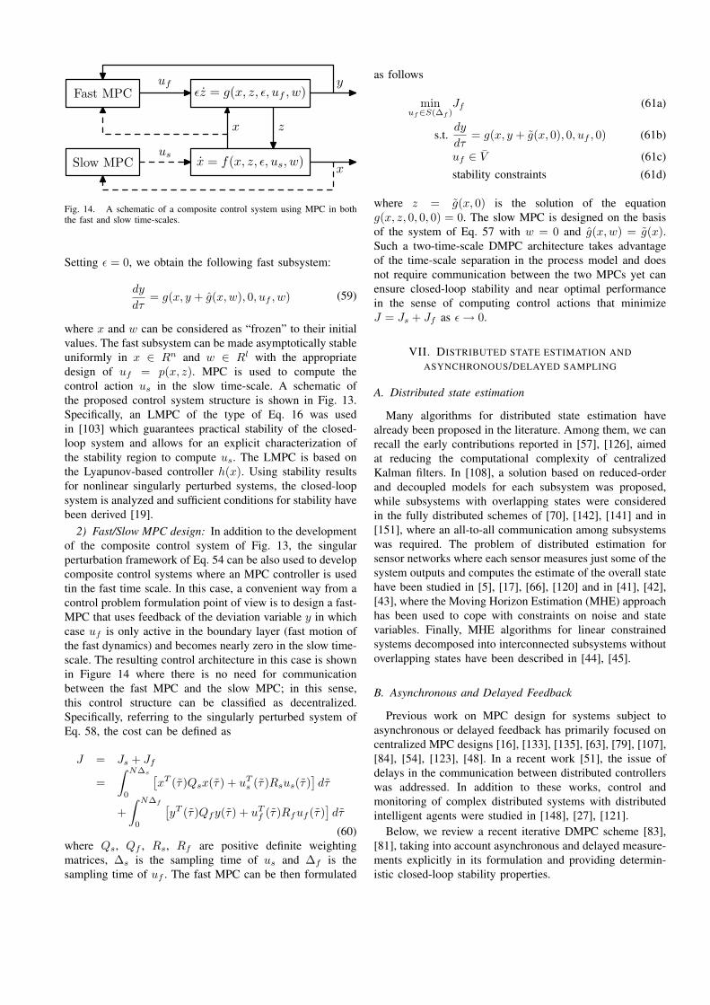
Fig. 13. A schematic of a composite control system using MPC in theslow time-scale.

with MPC and allowing for reconfiguration of the controlstructure have also been reported in [122], [155]. As anadditional remark, it is worth mentioning that a recent streamof research is devoted to the so-called economic MPC, withthe aim to directly use feedback control for optimizingeconomic performance, rather than simply stabilizing theplant and maintaining steady operation, see e.g. [127], [34],[58].

In a wider perspective, hierarchical and multilayer struc-tures are useful for control of very large scale systemscomposed by a number of autonomous or semi-autonomoussubsystems, which must be coordinated to achieve a com-mon goal. Examples can be found in many different fields,such as robotics [8], [152], transportation networks [114],voltage control in energy distribution networks [115], con-trol of irrigation canals [116], [161], and automation ofbaggage handling systems [147]. The design of multilayerstructures according to a leader-follower approach for net-worked control has been considered in [7]. In any case,the design of multilayer structures requires multi-level andmulti-resolution models, which, according to [149], canbe obtained according to a functional, temporal or spatialdecomposition approach.

C. MPC of Two-Time-Scale Systems

Most chemical processes involve physico-chemical phe-nomena that occur in distinct (slow and fast) time scales.Singular perturbation theory provides a natural frameworkfor modeling, analyzing and controlling multiple time-scaleprocesses. While there has been extensive work on feedbackcontrol of two-time-scale processes within the singular per-turbation framework (e.g., [72]), results on MPC of two-time-scale systems have been relatively recent [153], [19].Below, we discuss some of these results pertaining to thesubject of decentralized/distributed MPC.

1) Slow time-scale MPC: Specifically, in [19], MPC wasconsidered in the context of nonlinear singularly perturbedsystems in standard form with the following state-spacedescription:

x = f(x, z, ε, us, w), x(0) = x0

εz = g(x, z, ε, uf , w), z(0) = z0

(54)

where x ∈ Rn and z ∈ Rm denote the vector of statevariables, ε is a small positive parameter, w ∈ Rl denotes the

vector of disturbances and us ∈ U ⊂ Rp and uf ∈ V ⊂ Rq

are two sets of manipulated inputs. Since the small parameterε multiplies the time derivative of the vector z in the systemof Eq. 2, the separation of the slow and fast variables inEq. 2 is explicit, and thus, we will refer to the vector x asthe slow states and to the vector z as the fast states. Withrespect to the control problem formulation, the assumptionis made that the fast states z are sampled continuously andtheir measurements are available for all time t (for exam-ple, variables for which fast sampling is possible usuallyinclude temperature, pressure and hold-ups) while the slowstates x are sampled synchronously and are available attime instants indicated by the time sequence tk≥0 withtk = t0 + k∆, k = 0, 1, . . . where t0 is the initial timeand ∆ is the sampling time (for example, slowly sampledvariables usually involve species concentrations). The setof manipulated inputs uf is responsible for stabilizing thefast dynamics of Eq. 2 and for this set the control actionis assumed to be computed continuously, while the set ofmanipulated inputs us is evaluated at each sampling timetk and is responsible for stabilizing the slow dynamics andenforcing a desired level of optimal closed-loop performance.The explicit separation of the slow and fast variables in thesystem of Eq. 2 allows decomposing it into two separatereduced-order systems evolving in different time-scales. Toproceed with such a two-time-scale decomposition and inorder to simplify the notation of the subsequent development,we will first address the issue of stability of the fast dynam-ics. Since there is no assumption that the fast dynamics ofEq. 2 are asymptotically stable, we assume the existence of a“fast” feedback control law uf = p(x, z) that renders the fastdynamics asymptotically stable. Substituting uf = p(x, z) inEq. 2 and setting ε = 0 in the resulting system, we obtain:

dx

dt= f(x, z, 0, us, w) (55a)

0 = g(x, z, 0, p(x, z), w) (55b)

Assuming that the equation g(x, z, 0, p(x, z), w) = 0 pos-sesses a unique root

z = g(x,w) (56)

we can construct the slow subsystem:

dx

dt= f(x, g(x,w), 0, us, w) =: fs(x, us, w) (57)

Introducing the fast time scale τ =t

εand the deviation

variable y = z − g(x,w), we can rewrite the nonlinearsingularly perturbed system of Eq. 2 as follows:

dx

dτ= εf(x, y + g(x,w), ε, us, w)

dy

dτ= g(x, y + g(x,w), ε, uf , w)− ε

∂g

∂ww

−ε∂g

∂xf(x, y + g(x,w), ε, us, w)

(58)

Fast MPC

Slow MPC

εz = g(x, z, ε, uf , w)

x = f(x, z, ε, us, w)

uf

us

x z

y

x

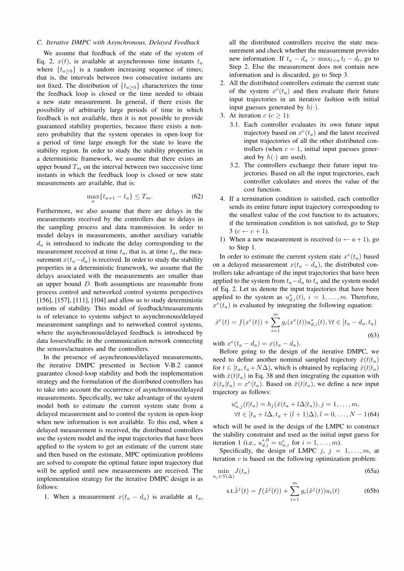
Fig. 14. A schematic of a composite control system using MPC in boththe fast and slow time-scales.

Setting ε = 0, we obtain the following fast subsystem:

dy

dτ= g(x, y + g(x,w), 0, uf , w) (59)

where x and w can be considered as “frozen” to their initialvalues. The fast subsystem can be made asymptotically stableuniformly in x ∈ Rn and w ∈ Rl with the appropriatedesign of uf = p(x, z). MPC is used to compute thecontrol action us in the slow time-scale. A schematic ofthe proposed control system structure is shown in Fig. 13.Specifically, an LMPC of the type of Eq. 16 was usedin [103] which guarantees practical stability of the closed-loop system and allows for an explicit characterization ofthe stability region to compute us. The LMPC is based onthe Lyapunov-based controller h(x). Using stability resultsfor nonlinear singularly perturbed systems, the closed-loopsystem is analyzed and sufficient conditions for stability havebeen derived [19].

2) Fast/Slow MPC design: In addition to the developmentof the composite control system of Fig. 13, the singularperturbation framework of Eq. 54 can be also used to developcomposite control systems where an MPC controller is usedtin the fast time scale. In this case, a convenient way from acontrol problem formulation point of view is to design a fast-MPC that uses feedback of the deviation variable y in whichcase uf is only active in the boundary layer (fast motion ofthe fast dynamics) and becomes nearly zero in the slow time-scale. The resulting control architecture in this case is shownin Figure 14 where there is no need for communicationbetween the fast MPC and the slow MPC; in this sense,this control structure can be classified as decentralized.Specifically, referring to the singularly perturbed system ofEq. 58, the cost can be defined as

J = Js + Jf

=∫ N∆s

0

[xT (τ)Qsx(τ) + uT

s (τ)Rsus(τ)]dτ

+∫ N∆f

0

[yT (τ)Qfy(τ) + uT

f (τ)Rfuf (τ)]dτ

(60)where Qs, Qf , Rs, Rf are positive definite weightingmatrices, ∆s is the sampling time of us and ∆f is thesampling time of uf . The fast MPC can be then formulated

as follows

minuf∈S(∆f )

Jf (61a)

s.t.dy

dτ= g(x, y + g(x, 0), 0, uf , 0) (61b)

uf ∈ V (61c)stability constraints (61d)

where z = g(x, 0) is the solution of the equationg(x, z, 0, 0, 0) = 0. The slow MPC is designed on the basisof the system of Eq. 57 with w = 0 and g(x,w) = g(x).Such a two-time-scale DMPC architecture takes advantageof the time-scale separation in the process model and doesnot require communication between the two MPCs yet canensure closed-loop stability and near optimal performancein the sense of computing control actions that minimizeJ = Js + Jf as ε → 0.

VII. DISTRIBUTED STATE ESTIMATION ANDASYNCHRONOUS/DELAYED SAMPLING

A. Distributed state estimation

Many algorithms for distributed state estimation havealready been proposed in the literature. Among them, we canrecall the early contributions reported in [57], [126], aimedat reducing the computational complexity of centralizedKalman filters. In [108], a solution based on reduced-orderand decoupled models for each subsystem was proposed,while subsystems with overlapping states were consideredin the fully distributed schemes of [70], [142], [141] and in[151], where an all-to-all communication among subsystemswas required. The problem of distributed estimation forsensor networks where each sensor measures just some of thesystem outputs and computes the estimate of the overall statehave been studied in [5], [17], [66], [120] and in [41], [42],[43], where the Moving Horizon Estimation (MHE) approachhas been used to cope with constraints on noise and statevariables. Finally, MHE algorithms for linear constrainedsystems decomposed into interconnected subsystems withoutoverlapping states have been described in [44], [45].

B. Asynchronous and Delayed Feedback

Previous work on MPC design for systems subject toasynchronous or delayed feedback has primarily focused oncentralized MPC designs [16], [133], [135], [63], [79], [107],[84], [54], [123], [48]. In a recent work [51], the issue ofdelays in the communication between distributed controllerswas addressed. In addition to these works, control andmonitoring of complex distributed systems with distributedintelligent agents were studied in [148], [27], [121].

Below, we review a recent iterative DMPC scheme [83],[81], taking into account asynchronous and delayed measure-ments explicitly in its formulation and providing determin-istic closed-loop stability properties.

C. Iterative DMPC with Asynchronous, Delayed Feedback

We assume that feedback of the state of the system ofEq. 2, x(t), is available at asynchronous time instants tawhere ta≥0 is a random increasing sequence of times;that is, the intervals between two consecutive instants arenot fixed. The distribution of ta≥0 characterizes the timethe feedback loop is closed or the time needed to obtaina new state measurement. In general, if there exists thepossibility of arbitrarily large periods of time in whichfeedback is not available, then it is not possible to provideguaranteed stability properties, because there exists a non-zero probability that the system operates in open-loop fora period of time large enough for the state to leave thestability region. In order to study the stability properties ina deterministic framework, we assume that there exists anupper bound Tm on the interval between two successive timeinstants in which the feedback loop is closed or new statemeasurements are available, that is:

maxata+1 − ta ≤ Tm. (62)

Furthermore, we also assume that there are delays in themeasurements received by the controllers due to delays inthe sampling process and data transmission. In order tomodel delays in measurements, another auxiliary variableda is introduced to indicate the delay corresponding to themeasurement received at time ta, that is, at time ta, the mea-surement x(ta−da) is received. In order to study the stabilityproperties in a deterministic framework, we assume that thedelays associated with the measurements are smaller thanan upper bound D. Both assumptions are reasonable fromprocess control and networked control systems perspectives[156], [157], [111], [104] and allow us to study deterministicnotions of stability. This model of feedback/measurementsis of relevance to systems subject to asynchronous/delayedmeasurement samplings and to networked control systems,where the asynchronous/delayed feedback is introduced bydata losses/traffic in the communication network connectingthe sensors/actuators and the controllers.

In the presence of asynchronous/delayed measurements,the iterative DMPC presented in Section V-B.2 cannotguarantee closed-loop stability and both the implementationstrategy and the formulation of the distributed controllers hasto take into account the occurrence of asynchronous/delayedmeasurements. Specifically, we take advantage of the systemmodel both to estimate the current system state from adelayed measurement and to control the system in open-loopwhen new information is not available. To this end, when adelayed measurement is received, the distributed controllersuse the system model and the input trajectories that have beenapplied to the system to get an estimate of the current stateand then based on the estimate, MPC optimization problemsare solved to compute the optimal future input trajectory thatwill be applied until new measurements are received. Theimplementation strategy for the iterative DMPC design is asfollows:

1. When a measurement x(ta − da) is available at ta,

all the distributed controllers receive the state mea-surement and check whether the measurement providesnew information. If ta − da > maxl<a tl − dl, go toStep 2. Else the measurement does not contain newinformation and is discarded, go to Step 3.

2. All the distributed controllers estimate the current stateof the system xe(ta) and then evaluate their futureinput trajectories in an iterative fashion with initialinput guesses generated by h(·).

3. At iteration c (c ≥ 1):3.1. Each controller evaluates its own future input

trajectory based on xe(ta) and the latest receivedinput trajectories of all the other distributed con-trollers (when c = 1, initial input guesses gener-ated by h(·) are used).

3.2. The controllers exchange their future input tra-jectories. Based on all the input trajectories, eachcontroller calculates and stores the value of thecost function.

4. If a termination condition is satisfied, each controllersends its entire future input trajectory corresponding tothe smallest value of the cost function to its actuators;if the termination condition is not satisfied, go to Step3 (c ← c + 1).

1) When a new measurement is received (a ← a+1), goto Step 1.

In order to estimate the current system state xe(ta) basedon a delayed measurement x(ta − da), the distributed con-trollers take advantage of the input trajectories that have beenapplied to the system from ta−da to ta and the system modelof Eq. 2. Let us denote the input trajectories that have beenapplied to the system as u∗d,i(t), i = 1, . . . ,m. Therefore,xe(ta) is evaluated by integrating the following equation:

xe(t) = f(xe(t)) +m∑

i=1

gi(xe(t))u∗d,i(t),∀t ∈ [ta − da, ta)

(63)with xe(ta − da) = x(ta − da).

Before going to the design of the iterative DMPC, weneed to define another nominal sampled trajectory x(t|ta)for t ∈ [ta, ta +N∆), which is obtained by replacing x(t|ta)with x(t|ta) in Eq. 38 and then integrating the equation withx(ta|ta) = xe(ta). Based on x(t|ta), we define a new inputtrajectory as follows:

uen,j(t|ta) = hj(x(ta + l∆|ta)), j = 1, . . . , m,

∀t ∈ [ta + l∆, ta + (l + 1)∆), l = 0, . . . , N − 1(64)

which will be used in the design of the LMPC to constructthe stability constraint and used as the initial input guess foriteration 1 (i.e., u∗,0d,i = ue

n,i for i = 1, . . . , m).Specifically, the design of LMPC j, j = 1, . . . , m, at

iteration c is based on the following optimization problem:

minuj∈S(∆)

J(ta) (65a)

s.t. ˙xj(t) = f(xj(t)) +m∑

i=1

gi(xj(t))ui(t) (65b)

ui(t) = u∗,c−1d,i (t|ta),∀i 6= j (65c)∥∥∥uj(t)− u∗,c−1

d,j (t|ta)∥∥∥ ≤ ∆uj ,

∀τ ∈ [ta, ta + ND,a∆) (65d)uj(t) ∈ Uj (65e)

xj(ta) = xe(ta) (65f)∂V (xj(t))

∂xj

(1m

f(xj(t)) + gj(xj(t))uj(t))

≤ ∂V (x(t|ta))∂x

(1m

f(x(t|ta)) + gj(x(t|ta))uen,j(t|ta)

),

∀t ∈ [ta, ta + ND,a∆) (65g)

where ND,a is the smallest integer satisfying ND,a∆ ≥ Tm+D−da. The optimal solution to this optimization problem isdenoted u∗,cd,j(a|ta) which is defined for t ∈ [ta, ta + N∆).Accordingly, we define the final optimal input trajectoryof LMPC j of Eq. 65 as u∗d,j(t|tk) which is also definedfor t ∈ [ta, ta + N∆). Note again that the length of theconstraint ND,a depends on the current delay da, so it mayhave different values at different time instants and has to beupdated before solving the optimization problems.

The manipulated inputs of the closed-loop system underthe above iterative DMPC for systems subject to delayedmeasurements are defined as follows:

ui(t) = u∗d,i(t|ta), i = 1, . . . , m, ∀t ∈ [ta, ta+q) (66)

for all ta such that ta − da > maxl<a tl − dl and fora given ta, the variable q denotes the smallest integerthat satisfies ta+q − da+q > ta − da. Recent work hasalso addressed the problem of communication disruptionsbetween the distributed controllers [59].

VIII. FUTURE RESEARCH DIRECTIONS

In this section, we discuss various topics for future re-search work in the area of DMPC; the list is not intended tobe exhaustive and it is certainly based on our experiences,biases and hopes.

A. DMPC: Loop Partitioning and Decompositions

While there have been several suggestions for how topartition the loops in a DMPC system (i.e., what specific con-trol actuators each MPC will manipulate) based on physicalarguments, insight into process dynamic behavior like, forexample, two-time-scale behavior [74], [65], or plant layoutconsiderations like one controller per plant unit, there is nogeneral framework for computing optimal (in a certain well-defined sense) input (control actuator) decompositions forDMPC. Undoubtedly, this problem is very hard in its fullgenerality, however, even solutions for large-scale systemsof specific structure, like linear systems [106], [1] or well-defined parts of a chemical plant flowsheet, could be veryuseful. Research in this direction should go hand-in-handwith the development of optimal communication strategiesbetween the distributed controllers so that controller evalu-ation time, communication network usage and closed-loopstability, performance and robustness are optimized.

B. Distributed State Estimation and DMPC

Most of the available DMPC schemes rely on the assump-tion of availability of measurements of the complete statevector. However, it is possible that a distributed controller ina large-scale control system may not have access to all themeasurements or that measurements of all the process statesare not available. In this case, in the design of the distributedcontrollers, we need to take into account that differentdistributed controllers may have access to measurements ofdifferent parts of the process states, so that methods forDMPC with partial state measurements are required. Futureresearch in this direction should take advantage of the avail-able distributed state estimation schemes reviewed in sectionVII of this paper and should look at how best the combina-tion of a DMPC algorithm with centralized/distributed stateestimators can be addressed. One approach is to design adifferent state observer for each controller (i.e., distributedstate estimation), while an alternative approach is to designa centralized observer that sends the estimated state to allthe distributed controllers. In this context, the integration ofthe state estimation schemes with the DMPC algorithms sothat desired levels of stability, performance and robustnessare attained in the closed-loop system should be rigorouslystudied.

C. Economic DMPC and distributed optimization

Most industrial process control applications are based onhierarchical control schemes in which first the operationpoint of the plant is determined based on economic, safetyand environmental considerations (usually using steady statemodels), and then process control systems are used to drivethe plant to this steady state (usually using dynamic models).There have been some recent advances in integrating eco-nomic optimization and process control in a single MPC us-ing centralized approaches, for example the MPC for trackingschemes proposed in [30], [47], [77] and the MPC schemesbased directly on an economic cost function proposed in [34],[62], [58]. It is clear that, for large scale systems, DMPCmay be an appropriate path to tackle the resulting economicoptimization problem. Furthermore, DMPC stands to benefitfrom distributed optimization schemes that are tailored tohandle DMPC optimization problems in an optimal fashionaccounting for control-loop decomposition, plant variableinteraction patterns and controller communication strategies.Research in this direction may start from the extension tothe distributed case of well-known techniques for centralizedMPC, such as the multiple shooting method.

D. DMPC and Hybrid systems

Hybrid systems constitute an important class of mathemat-ical models that explicitly account for the intricate couplingbetween continuous dynamics and discrete events. Whilethere has been extensive work over the last fifteen years onanalysis and control of hybrid systems (see, for example,[10], [25] and the references therein), distributed MPC ofhybrid systems is a research topic that has received noattention. In the context of chemical process control and

operations, due to changes in raw materials, energy sources,product specifications and market demands, and abrupt ac-tuator and sensor faults, it is possible to describe processbehavior with classes of switched nonlinear systems thatinvolve differential equation models whose right-hand-side isindexed with respect to different modes of operation. Froma controller design standpoint, in order to achieve closed-loop stability, discrete mode transition situations should becarefully accounted for in the control problem formulationand solution. In order to achieve mode transitions in anoptimal setting and accommodate input/state constraints,distributed model predictive control (MPC) framework canbe employed, particularly in cases where the computationalcomplexity of a centralized MPC may significantly increaseas the number of operational modes, control inputs and statesincreases.

E. Monitoring and reconfigurability of DMPC

Monitoring and reconfiguration of DMPC is an importantresearch topic. DMPC systems offer a vast set of possibilitiesfor reconfiguration in the event of sensor and actuatorfaults to maintain the desired closed-loop performance. Ina recent set of papers [23], [22], a data-based monitoringand reconfiguration system was developed for a distributedmodel predictive control system in the presence of controlactuator faults. In addition to a monitoring method, appropri-ate DMPC reconfiguration (fault-tolerant control) strategieswere designed to handle the actuator faults and maintain theclosed-loop system state within a desired operating region.There is certainly a lot more to be done in the context ofDMPC monitoring and fault-tolerance.

Furthermore, in addition to its importance in the contextof DMPC fault-tolerance, reconfigurability of DMPC couldprovide flexibility to the control system and could be ex-plored in the context of other areas as follows.

During steady-state operation, it is not necessary to con-tinuously transmit among the distributed estimation/controlagents. In fact, in the case where one system does not receiveany new information (and can be sure that no transmissionfaults have occurred), it can be assumed that the other agentsbasically maintain their previous state. This reduction ofthe information transmitted can be particularly significant insensor networks with local power supply in order to havesignificant energy savings, which could guarantee a longer“life” of the sensors and/or of the actuators.

For similar reasons, future research efforts could deal withthe so-called “plug and play” control as well as with DMPCscalability. In nominal operating conditions, the control sys-tem assumes a minimal configuration, while in perturbedconditions sensors and/or actuators are added. The challengehere is to avoid the redesign of the overall control system,in particular for the elements not directly dynamically con-nected with the additional sensors and actuators. The readermay refer to [105], [145], [71], [155] for some references on“plug and play” control.

In addition, moving from industrial plants to very large-scale systems, such as transportation or distribution net-

works, or to the so-called “System-of-Systems” (i.e., verylarge-scale infrastructures of interacting subsystems, whichare by themselves composed of large-scale and complexsystems; see, for example, [93]), with operational and man-agerial independence, it is clear that the problem of recon-figuration of the control system is fundamental to cope withchanging requirements. For these systems, also the problemof partitioning and clustering is a very important one (recentwork can be found in [118]). In general, there is a substantiallack of methodologies for appropriate temporal and spatialpartitions and for the development of consistent multi-level,multi-scale models for DMPC design.

F. Applications

DMPC has a lot to offer in the context of industrial processcontrol practice. As plants become increasingly automatedwith advanced model-based control systems and the adoptionof advanced communication networks together with the as-sociated sensors and actuators continuous to broaden, DMPCcould provide the framework for the design of the next-generation, distributed model-based control systems. But theimpact of DMPC could go well-beyond industrial processcontrol practice and could become the method of choicefor the design of control systems for the individual com-ponenets/subsystems of large-scale, heterogenous distributednetworks (like, for example, “smart grid”-type networkswhere numerous renewables-based energy generation sys-tems are coupled with the electric grid and “smart” loads). Itis our hope that this paper will contribute towards developingfurther DMPC theory and practice.

REFERENCES

[1] W. Al-Gherwi, H. Budman, and A. Elkamel. Selection of controlstructure for distributed model predictive control in the presence ofmodel errors. Journal of Process Control, 20:270–284, 2010.

[2] A. Alessio, D. Barcelli, and A. Bemporad. Decentralized modelpredictive control of dynamically coupled linear systems. Journal ofProcess Control, 21:705–714, 2011.

[3] A. Alessio and A. Bemporad. Stability conditions for decentralizedmodel predictive control under packet drop communication. InProceedings of the American Control Conference, pages 3577–3582,Seattle, Washington, 2008.

[4] F. Allgower and F. J. Doyle. Nonlinear process control - which wayto the promised land? In Proceedings of 5th International Conferenceon Chemical Process Control, pages 24–45, Tahoe City, CA, 1997.

[5] P. Alriksson and A. Rantzer. Distributed Kalman filtering usingweighted averaging. In Proceedings of the 17th International Sym-posium on Mathematical Theory of Networks and Systems, Kyoto,Japan, 2006.

[6] I. Alvarado, D. Limon, D. Munoz de la Pena, J. M. Maestre, M. A.Ridao, H. Scheu, W. Marquardt, R. R. Negenborn, B. De Schutter,F. Valencia, and J. Espinosa. A comparative analysis of distributedMPC techniques applied to the HD-MPC four tank benchmark.Journal of Process Control, 21:800–815, 2011.

[7] T. Bacar and R. Srikant. A Stackelberg network game with alarge number of followers. Journal of Optimization, Theory andApplications, 115:479–490, 2002.

[8] A. D. Baker. A survey of factory control algorithms that can beimplemented in a multi-agent heterarchy: Dispatching, scheduling,and pull. Journal of Manufacturing Systems, 17:297–320, 1998.

[9] L. Bakule. Decentralized control: An overview. Annual Reviews inControl, 32:87–98, 2008.

[10] A. Bemporad and M. Morari. Control of systems integrating logic,dynamics and constraints. Automatica, 35:407–427, 1999.

[11] D. P. Bertsekas and J. N. Tsitsiklis. Parallel and DistributedComputation. Athena Scinetific, Belmont, Massachusetts, 1997.

[12] R. R. Bitmead, M. Gevers, and V. Wertz. Adaptive Optimal Control– The Thinking Man’s GPC. Prentice-Hall, Englewood Cliffs, NJ,1990.

[13] E.F. Camacho and C. Bordons. Model Predictive Control. SpringerVerlag, 2004.

[14] E. Camponogara and B. Barcelos de Oliveira. Distributed optimiza-tion for model predictive control of linear-dynamic networks. IEEETransactions on Systems, Man, and Cybernetics, Part A: Systems andHumans, 39:1331–1338, 2009.

[15] E. Camponogara, D. Jia, B. H. Krogh, and S. Talukdar. Distributedmodel predictive control. IEEE Control Systems Magazine, 22:44–52,2002.

[16] P. Carini, R. Micheli, and R. Scattolini. Multirate self-tuningpredictive control with application to a binary distillation column.International Journal of Systems Science, 21:51–64, 1990.

[17] R. Carli, A. Chiuso, L. Schenato, and S. Zampieri. DistributedKalman filtering based on consensus strategies. IEEE Journal onSelected Areas in Communications, 26:622–633, 2008.

[18] H. Chen and F. Allgower. A quasi-infinite horizon nonlinear modelpredictive control scheme with guaranteed stability. Automatica,34:1205–1217, 1998.

[19] X. Chen, M. Heidarinejad, J. Liu, D. Munoz de la Pena, andP. D. Christofides. Model predictive control of nonlinear singularlyperturbed systems: Application to a large-scale process network.Journal of Process Control, 21:1296–1305, 2011.

[20] R. Cheng, J. F. Forbes, and W.S. Yip. Price-driven coordinationmethods for solving plant-wide MPC problems. Journal of ProcessControl, 17:429–438, 2007.

[21] R. Cheng, J. F. Forbes, and W.S. Yip. Dantzig-Wolfe decomposi-tion and plant-wide MPC coordination. Computers and ChemicalEngineering, 32:1507–1522, 2008.

[22] D. Chilin, J. Liu, J. F. Davis, and P. D. Christofides. Data-basedmonitoring and reconfiguration of a distributed model predictivecontrol system. International Journal of Robust and NonlinearControl, in press.

[23] D. Chilin, J. Liu, D. Munoz de la Pena, P. D. Christofides, andJ. F. Davis. Detection, isolation and handling of actuator faultsin distributed model predictive control systems. Journal of ProcessControl, 20:1059–1075, 2010.

[24] P. D. Christofides, J. F. Davis, N. H. El-Farra, D. Clark, K. R. D.Harris, and J. N. Gipson. Smart plant operations: Vision, progressand challenges. AIChE Journal, 53:2734–2741, 2007.

[25] P. D. Christofides and N. H. El-Farra. Control of nonlinear andhybrid process systems: Designs for uncertainty, constraints andtime-delays. Springer-Verlag, Berlin, Germany, 2005.

[26] P. D. Christofides, J. Liu, and D. Munoz de la Pena. Networked andDistributed Predictive Control: Methods and Nonlinear Process Net-work Applications. Advances in Induatrial Control Series. Springer-Verlag, London, England, 2011.

[27] A. Cinar, A. Palazoglu, and F. Kayihan. Chemical Process Perfor-mance Evaluation. CRC Press-Taylor & Francis, Boca Raton, FL,2007.

[28] F. Clarke, Y. Ledyaev, and E. Sontag. Asymtotic controllabilityimplies feedback stabilization. IEEE Transactions on AutomaticControl, 42:1394–1407, 1997.

[29] H. Cui and E. W. Jacobsen. Performance limitations in decentralizedcontrol. Journal of Process Control, 12:485–494, 2002.

[30] Limon D., I. Alvarado, T. Alamo, and E.F. Camacho. MPC fortracking piecewise constant references for constrained linear systems.Automatica, 44:2382 – 2387, 2008.

[31] J. F. Davis. Report from NSF Workshop on Cyberinfrastructurein Chemical and Biological Systems: Impact and Directions, (seehttp://www.oit.ucla.edu/nsfci/NSFCIFullReport.pdf for the pdf file ofthis report). Technical report, 2007.

[32] E. J. Davison and T. N. Chang. Decentralized stabilization andpole assisgnment for general proper systems. IEEE Transactionson Automatic Control, 35:652–664, 1990.

[33] G. De Nicolao, L. Magni, and R. Scattolini. Stabilizing receding-horizon control of nonlinear time-varying systems. IEEE Trans. onAutomatic Control, AC-43:1030–1036, 1998.

[34] M. Diehl, R. Amrit, and J. B. Rawlings. A Lyapunov function foreconomic optimizing model predictive control. IEEE Transactionson Automatic Control, 56:703–707, 2011.

[35] M.D. Doan, T. Keviczky, and B. De Schutter. An iterative scheme fordistributed model predictive control using Fenchel’s duality. Journalof Process Control, 21:746–755, 2011.

[36] W. B. Dunbar. Distributed receding horizon control of dynamicallycoupled nonlinear systems. IEEE Transactions on Automatic Control,52:1249–1263, 2007.

[37] W. B. Dunbar and S. Desa. Distributed MPC for dynamic supplychain management. In Int. Workshop on Assessment and Future Di-rections of NMPC, Freudenstadt-Lauterbad, Germany, 26-30, 2005.

[38] W. B. Dunbar and R. M. Murray. Distributed receding horizon controlwith application to multi-vehicle formation stabilization. Automatica,42:549–558, 2006.

[39] Camponogara E., H. F. Scherer, and L. Vila Moura. Distributedoptimization for predictive control with input and state constraints:Preliminary theory and application to urban traffic control. In Pro-ceedings of the IEEE Int. Conf. on Systems, Man, and Cybernetics,pages 3726–3732, 2009.

[40] S. Engell. Feedback control for optimal process operation. Journalof Process Control, 17:203–219, 2007.

[41] M. Farina, G. Ferrari-Trecate, and R. Scattolini. Distributed movinghorizon estimation for sensor networks. In Proceedings of the 1stIFAC Workshop on Estimation and Control of Networked Systems,Venice, Italy, pages 126 – 131, 2009.

[42] M. Farina, G. Ferrari-Trecate, and R. Scattolini. Distributed movinghorizon estimation for linear constrained systems. IEEE Transactionson Automatic Control, 55:2462–2475, 2010.

[43] M. Farina, G. Ferrari-Trecate, and R. Scattolini. Distributed movinghorizon estimation for nonlinear constrained systems. In Proceedingsof the 8th IFAC Symposium on Nonlinear Control Systems, Bologna,Italy, 2010.

[44] M. Farina, G. Ferrari-Trecate, and R. Scattolini. Moving horizonstate estimation of large-scale constrained partitioned systems. Au-tomatica, 46:910 – 918, 2010.

[45] M. Farina, G. Ferrari-Trecate, and R. Scattolini. Moving horizonestimation for distributed nonlinear systems with application tocascade river reaches. Journal of Process Control, 21:767–774, 2011.

[46] M. Farina and R. Scattolini. Distributed non-cooperative MPC withneighbor-to-neighbor communication. In Proceedings of the 18thIFAC World Congress, Milan, Italy, 2011.

[47] A. Ferramosca, D. Limon, I. Alvarado, T. Alamo, and E.F. Camacho.MPC for tracking with optimal closed-loop performance. Automatica,45:1975 – 1978, 2009.

[48] R. Findeisen and P. Varutti. Stabilizing nonlinear predictive controlover nondeterministic communication networks. In Lalo Magni,Davide Raimondo, and Frank Allgwer, editors, Nonlinear ModelPredictive Control, volume 384 of Lecture Notes in Control andInformation Sciences, pages 167–179. Springer Berlin / Heidelberg,2009.

[49] W. Findeisen, F.N. Bailey, M. Brdys, K. Malinovski, P. Tatjewski,and A. Wozniak. Control and Coordination in Hierarchical Systems.Wiley and Sons, Ne York, 1980.

[50] F. A. Fontes. A general framework to design stabilizing nonlinearmodel predictive controllers. Systems & Control Letters, 42:127–143,2001.

[51] E. Franco, L. Magni, T. Parisini, M. M. Polycarpou, and D. M.Raimondo. Cooperative constrained control of distributed agents withnonlinear dynamics and delayed information exchange: A stabilizingreceding-horizon approach. IEEE Transactions on Automatic Control,53:324–338, 2008.

[52] C. E. Garcıa, D. M. Prett, and M. Morari. Model predictive control:Theory and practice–A survey. Automatica, 25:335–348, 1989.

[53] G. Grimm, M. J. Messina, S. E. Tuna, and A. R. Teel. Modelpredictive control: For want of a local control Lyapunov function,all is not lost. IEEE Transactions on Automatic Control, 50:546–558, 2005.

[54] L. Grune, J. Pannek, and K. Worthmann. A networked unconstrainednonlinear MPC scheme. In Proceedings of European Control Con-ference, pages 371–376, Budapest, Hungary, 2009.

[55] R. D. Gudi and J. B. Rawlings. Identification for decentralized modelpredictive control. AIChE Journal, 52:2198–2210, 2006.

[56] E. Gyurkovics and A. M. Elaiw. Stabilization of sampled-datanonlinear systems by receding horizon contyrol via discrete-timeapproximations. Automatica, 40:2017–2028, 2004.

[57] H.R. Hashemipour, S. Roy, and A.J. Laub. Decentralized structures

for parallel Kalman filtering. IEEE Transactions on AutomaticControl, 33:88 – 94, 1988.

[58] M. Heidarinejad, J. Liu, and P. D. Christofides. Economic modelpredictive control of nonlinear process systems using Lyapunovtechniques. AIChE Journal, in press.

[59] M. Heidarinejad, J. Liu, D. Munoz de la Pena, J. F. Davis, andP. D. Christofides. Handling communication disruptions in distributedmodel predictive control of nonlinear systems. Journal of ProcessControl, 21:173–181, 2011.

[60] M. Heidarinejad, J. Liu, D. Munoz de la Pena, J. F. Davis, and P. D.Christofides. Multirate Lyapunov-based distributed model predictivecontrol of nonlinear uncertain systems. Journal of Process Control,21:1231–1242, 2011.

[61] M. A. Henson and D. E. Seborg. Nonlinear Process Control.Prentice-Hall, Englewood Cliffs, NJ, 1997.

[62] R. Huang, E. Harinath, and L. T. Biegler. Lyapunov stability ofeconomically-oriented nmpc for cyclic processes. Journal of ProcessControl, 21:501–509, 2011.

[63] S. C. Jeong and P. Park. Constrained MPC algorithm for uncertaintime-varying systems with state-delay. IEEE Transactions on Auto-matic Control, 50:257–263, 2005.

[64] D. Jia and B. H. Krogh. Distributed model predictive control. InProceedings of the American Control Conference, pages 2767–2772,Arlington, VA, USA, 2001.

[65] S. S. Jogwar, M. Baldea, and P. Daoutidis. Dynamics and control ofprocess networks with large energy recycle. Industrial & EngineeringChemistry Research, 48:6087–6097, 2009.

[66] M. Kamgarpour and C. Tomlin. Convergence properties of a decen-tralized Kalman filter. Proceedings of the 47th IEEE Conference onDecision and Control, pages 3205 – 3210, 2008.

[67] M. R. Katebi and M. A. Johnson. Predictive control design for large-scale systems. Automatica, 33:421–425, 1997.

[68] T. Keviczky, F. Borrelli, and G. J. Balas. Decentralized recedinghorizon control for large scale dynamically decoupled systems.Automatica, 42:2105–2115, 2006.

[69] T. Keviczky, F. Borrelli, and K. Fregene. Decentralized recedinghorizon control and coordination of autonomous vehicle formations.IEEE Transactions on Control System Technology, 16:19–33, 2008.

[70] U. A. Khan and J. M. F. Moura. Distributing the Kalman filterfor large-scale systems. IEEE Transactions on Signal Processing,56:4919 – 4935, 2008.

[71] T. Knudsen, K. Trangbaek, and C.S. Kallesøe. Plug and play processcontrol applied to a district heating system. In Proceedings of the17th IFAC World Congress, Seoul, Korea, July 6-11 2008.

[72] P. Kokotovic, H. K. Khalil, and J. O’Reilly. Singular PerturbationMethods in Control: Analysis and Design. Academic Press, London,1986.

[73] C. Kravaris and Y. Arkun. Geometric nonlinear control - an overview.In Proceedings of 4th International Conference on Chemical ProcessControl, pages 477–515, Y. Arkun and W. H. Ray (Eds.), PadreIsland, TX, 1991.

[74] A. Kumar and P. Daoutidis. Nonlinear dynamics and control ofprocess systems with recycle. Journal of Process Control, 12:475–484, 2002.

[75] J. H. Lee. Recent advances in model predictive control and otherrelated areas. In Proceedings of 5th International Conference onChemical Process Control, pages 201–216, Tahoe City, CA, 1997.

[76] S. Li, Y. Zhang, and Q. Zhu. Nash-optimization enhanced distributedmodel predictive control applied to the shell benchmark problem.Information Science, 170:329–349, 2005.

[77] D. Limon, I. Alvarado, T. Alamo, and E.F. Camacho. Robust tube-based MPC for tracking of constrained linear systems with additivedisturbances. Journal of Process Control, 20:248 – 260, 2010.

[78] Y. Lin, E. D. Sontag, and Y. Wang. A smooth converse Lyapunovtheorem for robust stability. SIAM Journal on Control and Optimiza-tion, 34:124–160, 1996.

[79] G.-P. Liu, Y. Xia, J. Chen, D. Rees, and W. Hu. Networked predictivecontrol of systems with random networked delays in both forwardand feedback channels. IEEE Transactions on Industrial Electronics,54:1282–1297, 2007.

[80] J. Liu, X. Chen, D. Munoz de la Pena, and P. D. Christofides.Sequential and iterative architectures for distributed model predictivecontrol of nonlinear process systems. AIChE Journal, 56:2137–2149,2010.

[81] J. Liu, X. Chen, D. Munoz de la Pena, and P. D. Christofides.Iterative distributed model predictive control of nonlinear systems:Handling asynchronous, delayed measurements. IEEE Transactionson Automatic Control, in press.

[82] J. Liu, D. Munoz de la Pena, and P. D. Christofides. Distributed modelpredictive control of nonlinear process systems. AIChE Journal,55:1171–1184, 2009.

[83] J. Liu, D. Munoz de la Pena, and P. D. Christofides. Distributed modelpredictive control of nonlinear systems subject to asynchronous anddelayed measurements. Automatica, 46:52–61, 2010.

[84] J. Liu, D. Munoz de la Pena, P. D. Christofides, and J. F. Davis.Lyapunov-based model predictive control of nonlinear systems sub-ject to time-varying measurement delays. International Journal ofAdaptive Control and Signal Processing, 23:788–807, 2009.

[85] J. Maciejowski. Predictive Control with Constraints. Prentice-Hall,2001.

[86] U. Maeder, R. Cagienard, and M. Morari. Explicit model predictivecontrol. In S. Tarbouriech, G. Garcia, and A. H. Glattfelder, editors,Advanced Strategies in Control Systems with Input and OutputConstraints, Lecture Notes in Control and Information Sciences,volume 346, pages 237–271. Springer-Verlag, Berlin, 2007.

[87] J. M. Maestre, D. Munoz de la Pena, and E. F. Camacho. Distributedmodel predictive control based on a cooperative game. OptimalControl Applications and Methods, 32:153–176, 2011.

[88] J.M. Maestre, D. Munoz de la Pena, E.F. Camacho, and T. Alamo.Distributed model predictive control based on agent negotiation.Journal of Process Control, 21:685–697, 2011.

[89] L. Magni, G. De Nicolao, L. Magnani, and R. Scattolini. A stabilizingmodel-based predictive control for nonlinear systems. Automatica,37:1351–1362, 2001.

[90] L. Magni and R. Scattolini. Model predictive control of continuous-time nonlinear systems with piecewise constant control. IEEETransactions on Automatic Control, 49:900–906, 2004.

[91] L. Magni and R. Scattolini. Stabilizing decentralized model predictivecontrol of nonlinear systems. Automatica, 42:1231–1236, 2006.

[92] M. Mahmood and P. Mhaskar. Enhanced stability regions for modelpredictive control of nonlinear process systems. AIChE J., 54:1487–1498, 2008.

[93] M. W. Maier. Architecting principles for systems-of-systems. SystemsEngineering, 4:267–284, 1998.

[94] J. L. Massera. Contributions to stability theory. Annals of Mathe-matics, 64:182–206, 1956.

[95] D. Q. Mayne. Nonlinear model predictive control: An assessment.In Proceedings of 5th International Conference on Chemical ProcessControl, pages 217–231, Tahoe City, CA, 1997.

[96] D. Q. Mayne, J. B. Rawlings, C. V. Rao, and P. O. M. Scokaert.Constrained model predictive control: Stability and optimality. Au-tomatica, 36:789–814, 2000.

[97] D.Q. Mayne and H. Michalska. Receding horizon control of nonlin-ear systems. IEEE Transactions on Automatic Control, 35:814–824,1990.

[98] D.Q. Mayne, M.M. Seron, and S. V. Rakovic. Robust model predic-tive control of constrained linear systems with bounded disturbances.Automatica, 41:219–224, 2005.

[99] M. McKeon-Slattery. The world of wireless. Chemical EngineeringProgress, 106:6–11, 2010.

[100] M. Mercangoz and F. J. Doyle. Distributed model predictive controlof an experimental four-tank system. Journal of Process Control,17:297–308, 2007.

[101] M.D. Mesarovic, D. Macko, and Y. Takahara. Theory of Hierarchical,Multilevel, Systems. Academic Press, New York, 1970.

[102] P. Mhaskar, N. H. El-Farra, and P. D. Christofides. Predictive controlof switched nonlinear systems with scheduled mode transitions. IEEETransactions on Automatic Control, 50:1670–1680, 2005.

[103] P. Mhaskar, N. H. El-Farra, and P. D. Christofides. Stabilization ofnonlinear systems with state and control constraints using Lyapunov-based predictive control. Systems and Control Letters, 55:650–659,2006.

[104] P. Mhaskar, A. Gani, C. McFall, P. D. Christofides, and J. F. Davis.Fault-tolerant control of nonlinear process systems subject to sensorfaults. AIChE Journal, 53:654–668, 2007.

[105] A.G. Michelsen, R.I. Zamanabadi, and J. Stoustrup. Towards auto-matic model based controller design for reconfigurable plants. InProceedings of the 17th IFAC World Congress, Seoul, Korea, 2008.

[106] N. Motee and B. Sayyar-Rodsari. Optimal partitioning in distributedmodel predictive control. In Proceedings of the American ControlConference, pages 5300–5305, Minneapolis, Minnesota, 2006.

[107] D. Munoz de la Pena and P. D. Christofides. Lyapunov-based modelpredictive control of nonlinear systems subject to data losses. IEEETransactions on Automatic Control, 53:2076–2089, 2008.

[108] A. G. O. Mutambara. Decentralized estimation and control formultisensor systems. CRC Press, 1998.

[109] P. Mhaskar N. H. El-Farra and P. D. Christofides. Uniting boundedcontrol and MPC for stabilization of constrained linear systems.Automatica, 40:101–110, 2004.

[110] D. Nesic, A Teel, and P. Kokotovic. Sufficient conditions forstabilization of sampled-data nonlinear systems via discrete timeapproximations. Systems and Control Letters, 38:259–270, 1999.

[111] D. Nesic and A. R. Teel. Input-to-state stability of networked controlsystems. Automatica, 40:2121–2128, 2004.

[112] I. Necoara, V. Nedelcu, and I. Dumitrache. Parallel and distributedoptimization methods for estimation and control in networks. Journalof Process Control, 21:756–766, 2011.

[113] R. R. Negenborn. Multi-Agent Model Predictive Control withApplications to Power Networks. PhD thesis, Delft University ofTechnology, 2007.

[114] R. R. Negenborn, B. De Schutter, and J. Hellendoorn. Multi-agentmodel predictive control for transportation networks: Serial versusparallel schemes. Engineering Applications of Artificial Intelligence,21:353–366, 2008.

[115] R. R. Negenborn, S. Leirens, B. De Schutter, and J. Hellendoorn.Supervisory nonlinear MPC for emergency voltage control usingpattern search. Control Engineering Practice, 7:841–848, 2009.

[116] R. R. Negenborn, P. J. Van Overloop, T. Keviczky, and B. De Schut-ter. Distributed model predictive control of irrigation canals. Net-works and Heterogeneus Media, 4:359–380, 2009.

[117] P. Neumann. Communication in industrial automation: What is goingon? Control Engineering Practice, 15:1332–1347, 2007.

[118] C. Ocampo-Martinez, S. Bovo, and V. Puig. Partitioning approachoriented to the decentralised predictive control of large-scale systems.Journal of Process Control, 21:775–786, 2011.

[119] B. A. Ogunnaike and W. H. Ray. Process Dynamics, Modeling, andControl. Oxford University Press, New York, 1994.

[120] R. Olfati-Saber. Distributed Kalman filtering for sensor networks.Proceedings of the 46th IEEE Conference on Decision and Control,pages 5492 – 5498, 2007.

[121] S. Perk, F. Teymour, and A. Cinar. Statistical monitoring ofcomplex chemical processes using agent-based systems. Industrial& Engineering Chemistry Research, 49:5080–5093, 2010.

[122] B. Picasso, D. De Vito, R. Scattolini, and P. Colaneri. An MPCapproach to the design of two-layer hierarchical control systems.Automatica, 46:823–831, 2010.

[123] G. Pin and T. Parisini. Stabilization of networked control systemsby nonlinear model predictive control: A set invariance approach.In Lalo Magni, Davide Raimondo, and Frank Allgwer, editors,Nonlinear Model Predictive Control, volume 384 of Lecture Notes inControl and Information Sciences, pages 195–204. Springer Berlin /Heidelberg, 2009.

[124] D. M. Raimondo, L. Magni, and R. Scattolini. Decentralized MPC ofnonlinear system: An input-to-state stability approach. InternationalJournal of Robust and Nonlinear Control, 17:1651–1667, 2007.

[125] A. Rantzer. Dynamic dual decomposition for distributed control. InProccedings of the American Control Conference, pages 884–888,Saint Louis, Missouri, 2009.

[126] B. S. Rao and H. F. Durrant-Whyte. Fully decentralised algorithmfor multisensor Kalman filtering. IEE Proceedings on Control Theoryand Applications, D, 138:413–420, 1991.

[127] J. B. Rawlings, D. Bonne, J. B. Jørgensen, A. N. Venkat, and S. BayJørgensen. Unreachable setpoints in model predictive control. IEEETransactions on Automatic Control, 53:2209–2215, 2008.

[128] J. B. Rawlings and D. Q. Mayne. Model Predictive Control: Theoryand Design. Nob Hill Publishing, Madison, WI, 2009.

[129] J. B. Rawlings and B. T. Stewart. Coordinating multiple optimization-based controllers: New opportunities and challenges. Journal ofProcess Control, 18:839–845, 2008.

[130] A. Richards and J. P. How. Robust distributed model predictivecontrol. International Journal of Control, 80:1517–1531, 2007.

[131] J. A. Romagnoli and A. Palazoglu. Introduction to Process Control.CRC Press-Taylor & Francis, Boca Raton, FL, 2006.

[132] N. R. Sandell, P. Varajya, M. Athans, and M. C. Safonov. Surveyof decentralized control methods for large scale systems. IEEETransactions on Automatic Control, 23:108–128, 1978.

[133] R. Scattolini. A multirate self-tuning predictive controller for multi-variable systems. International Journal of Systems Science, 23:1347–1359, 1992.

[134] R. Scattolini. Architectures for distributed and hierarchical modelpredictive control - A review. Journal of Process Control, 19:723–731, 2009.

[135] R. Scattolini and N. Schiavoni. A multirate model based predictivecontroller. IEEE Transactions on Automatic Control, 40:1093–1097,1995.

[136] H. Scheu, J. Busch, and W. Marquardt. Nonlinear distributed dynamicoptimization based on first order sensitivities. In Proceedings of theAmerican Control Conference, pages 1574–1579, 2010.

[137] H. Scheu and W. Marquardt. Sensitivity-based coordination indistributed model predictive control. Journal of Process Control,21:715–728, 2011.

[138] D. E. Seborg, D. A. Mellichamp, T. F. Edgar, and F. J. Doyle. ProcessDynamics and Control. John Wiley & Sons, New York, 2010.

[139] D. D. Siljak. Decentralized Control of Complex Systems. AcademicPress, London, 1991.

[140] D. D. Siljak and A. I. Zecevic. Control of large-scale systems:Beyond decentralized feedback. Annual Reviews in Control, 29:169–179, 2005.

[141] S.S. Stankovic, M.S. Stankovic, and D.M. Stipanovic. Consensusbased overlapping decentralized estimation with missing observationsand communication faults. Automatica, 45:1397–1406, 2009.

[142] S.S. Stankovic, M.S. Stankovic, and D.M. Stipanovic. Consensusbased overlapping decentralized estimator. IEEE Transactions onAutomatic Control, 54:410–415, 2009.

[143] B. T. Stewart, A. N. Venkat, J. B. Rawlings, S. J. Wright, andG. Pannocchia. Coorperative distributed model predictive control.Systems and Control Letters, 59:460–469, 2010.

[144] B. T. Stewart, S. J. Wright, and J. B. Rawlings. Cooperativedistributed model predictive control for nonlinear systems. Journalof Process Control, 21:698–704, 2011.

[145] J. Stoustrup. Plug and play control: control technology towards newchallenges. European Journal of Control, 3:311–330, 2009.

[146] Y. Sun and N. H. El-Farra. Quasi-decentralized model-basednetworked control of process systems. Computers and ChemicalEngineering, 32:2016–2029, 2008.

[147] A. N. Tarau, B. De Schutter, and J. Hellendoorn. Model-based controlfor route choice in automated baggage handling systems. IEEETransactions on Systems, Man, and Cybernetics, Part C: Applicationsand Reviews, 40:341–351, 2010.

[148] E. Tatara, A. Cinar, and F. Teymour. Control of complex distributedsystems with distributed intelligent agents. Journal or ProcessControl, 17:415–427, 2007.

[149] P. Tatjewski. Advanced control and on-line process optimization inmultilayer structures. Annual Reviews in Control, 32:71–85, 2008.

[150] P. Trodden and A. Richards. Robust distributed model predictivecontrol using tubes. In Proceedings of the American ControlConference, pages 2034–2039, Minneapolis, Minnesota, 2006.

[151] R. Vadigepalli and F.J. Doyle. A distributed state estimation andcontrol algorithm for plantwide processes. IEEE Transactions onControl Systems Technology, 11:119 – 127, 2003.

[152] P. Valckenaers, H. Van Brussel, J. Wyns, P. Peeters, and L. Bongaerts.Multi-agent manufacturing control in holonic manufacturing systems.Human Systems Management, 18:233–243, 1999.

[153] E. J. Van Henten and J. Bontsema. Time-scale decomposition of anoptimal control problem in greenhouse climate management. ControlEngineering Practice, 17:88–96, 2009.

[154] A. N. Venkat, J. B. Rawlings, and S. J. Wright. Stability andoptimality of distributed model predictive control. In Proceedings ofthe 44th IEEE Conference on Decision and Control and the EuropeanControl Conference, pages 6680–6685, Seville, Spain, 2005.

[155] D. De Vito, B. Picasso, and R. Scattolini. On the design ofreconfigurable two-layer hierarchical control systems with MPC. InProceedings of the American Control Conference, pages 4707–4712,Baltimore, Maryland, 2010.

[156] G. Walsh, O. Beldiman, and L. Bushnell. Asymptotic behaviorof nonlinear networked control systems. IEEE Transactions onAutomatic Control, 46:1093–1097, 2001.

[157] G. Walsh, H. Ye, and L. Bushnell. Stability analysis of networkedcontrol systems. IEEE Transactions on Control Systems Technology,10:438–446, 2002.

[158] S.-H. Wang and E. J. Davision. On the stabilization of decentralizedcontrol systems. IEEE Transactions on Automatic Control, AC-18:473–478, 1973.

[159] E. B. Ydstie. Certainty equivalence adaptive control: Paradigms puz-zles and switching. In Proceedings of 5th International Conferenceon Chemical Process Control, pages 9–23, Tahoe City, CA, 1997.

[160] E. B. Ydstie. New vistas for process control: Integrating physics andcommunication networks. AIChE Journal, 48:422–426, 2002.

[161] A. Zafra-Cabeza, J.M. Maestre, M.A. Ridao, E.F. Camacho, andL. Sanchez. A hierarchical distributed model predictive controlapproach to irrigation canals: A risk mitigation perspective. Journalof Process Control, 21:787–799, 2011.

[162] Y. Zhang and S. Li. Networked model predictive control basedon neighbourhood optimization for serially connected large-scaleprocesses. Journal of Process Control, 17:37–50, 2007.

[163] P. Zornio and B. Karschnia. Realizing the promise of wireless.Chemical Engineering Progress, 105:22–29, 2009.